Marginal Notes for Kanatani’s

‘Statistical Optimization

for Geometric Computation’

editor: Leo Dorst

November 6, 2009

1 Introduction (Self)

Explanation of the book title:

• geometric: models and constraints

• optimization: theoretical accuracy bounds

• statistical: reliability

• computation: efficiency issues

Language:

• small noise in geometric models:

• perturbation theory on manifolds

1

2 Fundamentals of Linear Algebra(Leo Dorst)

Much for future reference, but let us identify newish elements.

2.1 Vector and Matrix Calculus

• Pg. 33: Cute notation for the cross product operator:

more usual → a× ≡

0 −a3 a2

a3 0 −a1

−a2 a1 0

= a× I ← new to me

Thena× x = a× x = (a× I) x.

Of course the cross product is very 3-D, and has rather awkward linearalgebra:

a 7→ f(a), b 7→ f(b)

butf(a× b) = det(f)f−>(a× b) 6= f(a)× f(b).

So the transformation of a normal vector is not the normal vector of thetransformation.1

• Pg. 35: Beware of Kanatani’s notation: Pn is not the projection onto nbut the projection to the hyperplane characterized by the normal vectorn (so perpendicular to n). For the projection onto the n-line he would usePn (see just below his (2.122)).

• Pg. 36: In (2.56) one would expect Kanatani to use Rodrigues’ formulafor a rotation matrix, since it matches his cross product treatment. For aunit rotation axis n, some equivalent forms are:

R = I cos(Ω) + sin(Ω) n× +(1− cos(Ω)

)nn> (the usual form)

= I + sin(Ω) n× +(1− cos(Ω)

)(n×)2 (a variation)

= I + sin(Ω) (n× I) +(1− cos(Ω)

)(n× I)2 (a Kanatani-like form).

Still, there are more convenient rotation representations such as quater-nions (fewer parameters, easier constraints), and rotors (generalized quater-nions in geometric algerba)2. Modern optimization of rotations often usesquaternions.

1Buy [3], and from now on use a∧b instead (since f(a∧b) = f(a)∧ f(b) and it works inn-D). Geez, how often do I have to tell you?

2In Euclidean geometric algebra, the universal rotation operator (rotor) isR = exp(n?Ω/2).In conformal geometric algebra, the universal rotation operator (rotor) is R = exp(Λ∗Ω/2),where Λ is the unit rotation axis, not necessarily through the origin.

2

[[[ insert Figure ]]]

Figure 1: The four fundamental subspaces of a linear transformation.

2.2 Eigenvalue Problem

In all the treatment of linear transformations and their matrices, it it is helpfulto realize that there are 4 fundamental spaces to each m× n matrix A of rankr (i.e. to each linear mapping):

• the n− r dimensional kernel of A (aka nullspace of A)

• the r dimensional image of A (aka column space of A, or range of A)

• the m− r dimensional kernel of A> (aka nullspace of A>)

• the r dimensional image of A> (aka row space of A, or range of A>)

The mapping A is invertible only for its r-dimensional image. The inverse thereis the pseudo-inverse. The SVD brings the latter into a particularly convenientform, since it gives each of the spaces an orthonormal basis. We recommendreading the SVD part in section (2.3) first, since it is more general, and thengoing back to special matrices such as square n × n and symmetric squarematrices treated in section (2.2). It gives more generic understanding.

2.3 Linear Systems and Optimization

• Pg. 45 Remember what is behind the SVD: find a frame of orthogonalvectors ui whose images under an m × n matrix A are also orthogonal.Such a frame can be found as the eigenvectors of A>A. This is easilyproved:

(Aui) · (Auj) = (Aui)>(Auj) = u>i A>Auj = u>i σjuj = σj ui · uj . (1)

So the originals ui and uj are orthogonal precisely when the images Auiand Auj are.3

Take the ui (i = 1, · · · , n) to be unit vectors and define their imagesthrough

Aui = λi vi, (2)

with the unit vectors vi (i = 1, · · · ,m) forming an orthonormal basis.Then λi are the singular values, and λi =

√σi. (See remark about unusual

Kanatani notation above).

Since A>A is symmetric (why?), the σi are real; since A>A is semi-positivedefinite (why?), the σi are non-negative; so the singular values λi are all

3Note that Kanatani swaps the notation of λi and σi: usually the σi are the singularvalues (that is why they have an s-like symbol!) and the λi the eigenvalues of A>A (it is soin [2]; he also has u and v opposite...

3

[[[ insert Figure ]]]

Figure 2: The SVD visualized.

non-negative and can be ordered. We define the m × n matrix Λ to bezero except on its diagonal, where the singular values are in descendingorder. For a 2× 3 matrix A, for instance:

Λ =(λ1 0 00 λ2 0

).

We can convert eq.(2) to matrix form as:

AU = V Λ, so A = V ΛU>,

with V and U orthogonal m×m and n×n matrices, respectively, orderedto correspond to the singular values. Details see Bretscher [2]. A figureshows these aspects: A is a diagonal Λ (only a stretching of the axes) ina well-chosen representation (related to the eigenvectors of A>A, as weshowed). Dimensions can also be reduced (this is the kernel of A) or added(this is the kernel of A>). One gets the original A back by rotating thedomain of Λ by U , and the range of Λ by V .

• Pg. 47: So, now the pseudoinverse in these terms: the 4 fundamentalspaces of the m × n matrix A of rank r (we use ONB for OrthoNormalBasis):

– the r-D image of A (RA) has as ONB the first r columns of V

– the r-D image of A> has as ONB the first r columns of U

– the (n − r)-D kernel of A (NA) has as ONB the last n − r columnsof U

– the (m− r)-D kernel of A> has as ONB the last m− r columns of V

Only the first r entries on the diagonal of Λ are non-zero. So we can notquite do the naive:

A−1 = (V ΛU>)−1 = UΛ−1V >,

but it is close; we should do that for the first r entries; and of courseΛ need not be square. Therefore the pseudoinverse of A is obtained bychanging entry λi to 1/λi and swapping the roles of U and V :

A− =r∑i=1

uiv>iλi

. Kanatani (2.121)

The rank-constrained inverse is just a variation on this theme, for numer-ical applications.

4

• Pg. 49: Referring back to a remark Kanatani makes in the introduction,least squares fitting of a line to data minimizes the sum of the squares ofthe vertical (y) distances and is not suitable for isotropic geometry. Thismethod needs to be modified to minimize the perpendicular distances tothe line independent of a coordinate system. He will treat line fitting inSection 10.1.

2.4 Matrix and Tensor Algebra

This is just notation, for now. To see if you understand, derive the factor of 2in (2.199).

5

3 Probabilities and Statistical Estimation (GwennEnglebienne)

Introductory remarks (see Gwenn’s slides):

• Frequentist approach

– The data comes from a distribution, let us find as best as we canwhich distribution that was.

– Find estimators for parameters, and try to figure out how good theseestimators are.

• Bayesian approach.

– The data could have come from any number of distributions, let usfind what those distributions could have been, and how likely theyare.

– Using Bayes rule does not make an approach Bayesian.

3.1 Probability Distributions

• Pg. 61: Expectation is a more general concept, of a functionf :

E[f(x)] =∫f(x) p(x) dx.

The mean is then the expectation of the data, setting f to the identityfunction.

• There is nothing yet in this chapter on estimating mean and the variancefrom the data. An unbiased estimator for the mean is as you would expect:

ˆx = 1N

∑i

xi.

An unbiased estimator for the variance has an unexpected normalization:

V [x] = 1N−1

∑i

(xi − x) (xi − x)>.

For a proof, see [[[ ?? ]]]. It should be noted that this is the estimatoryou use when you don’t know the mean; if you do know the mean, theunbiased estimator does use the division by N .

• Pg. 61: Definition of uncorrelated: the covariance of two variables is zero.E[(x − E[x]) (y − E[y])] = 0. If both variables have zero mean, they areuncorrelated if and only if E[x y] = E[x]E[y].

Definition of independent: the distribution of one variable does not affectthat of the other: p(x, y) = p(x)p(y).

Independent always implies uncorrelated. For a normal distrution, uncor-related implies independent, so that the two terms are equivalent then.

6

• Pg. 63: The derivative matrix occurring in (3.15) is the Jacobian. In(3.17) he calls ‘Pn the projection along n’, this ambiguous phrasing shouldbe interpreted as ‘the projection to the subspace perpendicular to n’.

• Pg. 64: In (3.27) that awkward projection notation again: PN is theprojection to the orthogonal complement of the null space of the tangentspace, and therefore projection to the tangent space.

Spectral decomposition of the covariance matrix is widely used. A typ-ical application of it is the so-called Karhunen-Loeve transform, betterknown as Principal Component Analysis (PCA). (BTW: that’s principal,not principle)

3.2 Manifolds and Local Distributions

• Pg. 67: Equation (3.29) is an approximation. The proper way for a man-ifold would be to define x as the location such that, for instance, the sumof squared distances along the manifold would be zero. E(x − x) is notmeasured along, and therefore not an intrinsic measure. To solve in theproper way (which Gijs Dubbelman has executed for rotation estimation),is to define geodesic length preserving mappings between manifold andtangent space at a location (these are called the exponential and loga-rithmic maps), and do an iterative algorithm to find the location x asdefined above. This method converges under certain conditions on themanifold, such as local compactness. However, Bishop [1] also uses (3.29)[[[ (Mises distribution term, Olaf?) ]]].

• Pg. 68: Try to derive (3.33) from (3.32). We could not, though [`×] [`×]> =I − ` `> is close. What seems to be going on is that Kanatani defines aquantitiy that has the same covariance as the target quantity but has asimpler form. Still, this is geometry, so precisely the point where we wouldhave appreciated more detail.

3.3 Gaussian Distributions and χ2 Distributions

• Pg. 68: Mahalanobis distance: Σ−1 effectively rescales the ellipsoids tospheres, or can be viewed as the metric involved in the dot product.

• Pg. 73: We can interpret (3.59) and also mode[R] = 2 − r as: evenfor large r, the χ2 distribution remains localized, around r with standarddeviation

√2r. In the χ2-test, this helps distinguish the distributions with

significantly different r. But Gwenn still calls it an ‘ugly hack’.

• Pg. 77: Misstatement: the likelihood is defined as p(x|θ) = f(θ), that is,viewed as a function of the parameters, not of the data.

7

3.4 Statistical Estimation for Gaussian Models

• Maximum Likelihood (ML) learning: Try to maximize prob of datagiven parameters, not prob of param given data Πip(yi|θ).For example, if we have N i.i.d. Gaussian distributed datapoints y1:N ,the probability of the data given the parameters is

p(y1:N |θ) =N∏i=1

n(yi; µ,Σ), (3)

where n(·; µ,Σ) indicates the Gaussian distribution with parameters meanµ and covariance Σ. Maximising this directly is difficult because of theproduct. However since ex is a monotonically increasing function, we cansimply maximise the log-likelihood instead:

log p(y1:N |θ) =N∑i=1

log n(yi; µ,Σ) (4)

Now we can take the first derivative and set this equal to zero. For illus-tration, we do this for the mean:

0 =∂

∂µ

[N∑i=1

(yi − µ)>Σ−1(yi − µ) + const

](5)

0 =N∑i=1

∂

∂µ(yi − µ)>Σ−1(yi − µ) (6)

0 = −2Σ−1N∑i=1

(yi − µ) (7)

0 =N∑i=1

yi −N∑i=1

µ (8)

µ =∑Ni=1 yiN

(9)

• Maximum a posteriori (MAP) learning: Problem ML: since we onlyhave final amounts of data, the distribution of the observed data is neverthe same as the distribution the data would have if we could observe itall.

We can therefore introduce prior knowledge about the parameters. Thatis, we optimise p(θ|y), which we obtain by:

p(θ|y) =p(y|θ)p(θ)

p(y)(10)

8

p(y) can be computed but is constant anyway, and does not affect themaximisation. Maximum a posteriori learning therefore reduces to max-imising log p(y1:N |θ) + log p(θ).

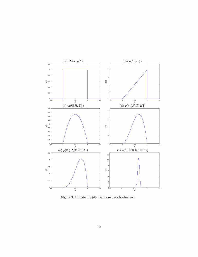
• The Bayesian approach: Here, we don’t maximise anything. We knowthat the data we observe may have come from many different distributions,but not all these distributions are equally likely. Instead of finding “themost probable distribution” for given observations, we keep a distributionover distributions.

As an example, consider coin toss giving head (Carsten’s phrasing) H(= 1)or tail T (= 0).4 We can parameterize the probability of a set of datapointsy = HHT with the Bernouilli distribution:

p(yi|θ) = θyi(1− θ)yi (11)

This gives us that p(H|θ) = θ and p(T |θ) = 1−θ. (As an exercise, confirmthat the ML estimate of θ =

∑i yi

N .) The Bayesian approach is to say thatwe don’t know θ, and we will never know it. But we do know that somevalues of θ are more likely than others. For example, if we see a sequenceof a hundred H and no T , we can probably infer that we have a cheater onour hands, and the coin isn’t fair (because of the law of large numbers).That is, we can associate a probability with each value of θ.5

So how can we compute p(θ|y1:N )? We use Bayes’ rule:

p(θ|H) =p(H|θ) p(θ)

p(H)(12)

p(H) =∫θ

p(H|θ)p(θ)dθ (13)

We first need to make assumptions about the value of θ. In this case,let us assume that we don’t know anything, except that 0 6 θ 6 1. Thecorresponding distribution over θ is plotted in Figure 3(a). If we observea H, we then use Bayes’ rule to update the distribution over θ, resultingin Figure 3(b). As more data is observed, the distribution over θ evolvesas depicted in the subsequent figures.

• Notice that Bayesian inference, Maximum a posteriori and MaximumLikelihood are identical in the limit of infinite amounts of data. Maxi-mum a Posteriori equals Maximum Likelihood if we assume an uniformprior (or have infinite amounts of data).

• Pg. 81: Kalman filter: In (3.104) the B appears superfluous, since if v isGaussian distributed, so is B in a straightforward manner, and vice versa.

4We do not work the example out analytically, because the functional form of the distri-butions becomes complicated and does not add anything to the understanding.

5In fact, the probability of any value of θ is zero, because θ is a continuous quantity.We therefore associate a probability density with it, which is normalised so that the integralbetween −∞ and ∞ equals 1. Details can be found in any basic text on probabilities.

9

(a) Prior p(θ) (b) p(θ|H)

0

0.2

0.4

0.6

0.8

1

1.2

-0.5 0 0.5 1 1.5

p(θ)

θ

0

0.5

1

1.5

2

-0.5 0 0.5 1 1.5

p(θ)

θ

(c) p(θ|H,T) (d) p(θ|H,T,H)

0

0.2

0.4

0.6

0.8

1

1.2

1.4

1.6

1.8

-0.5 0 0.5 1 1.5

p(θ)

θ

0

0.5

1

1.5

2

-0.5 0 0.5 1 1.5

p(θ)

θ

(e) p(θ|H,T,H,H) (f) p(θ|100 H, 50 T)

0

0.5

1

1.5

2

2.5

-0.5 0 0.5 1 1.5

p(θ)

θ

0

2

4

6

8

10

12

-0.5 0 0.5 1 1.5

p(θ)

θ

Figure 3: Update of p(θ|y) as more data is observed.

10

• Pg. 81 To use Kalman, you need to know the noise distributation v, wand a model A, C. Do all people using the Kalman filter really knowthat? Usually not. You have to estimate them, using the EM algorithm,or the Bayesian way (closed form). For more details, Chapter 13 in [1]

– About Kalman Filter techniques:A Kalman filter is just a Bayesian Network (though historically notso described). Notice that at each time step, the Kalman filter usesMAP (not Bayesian inference.)Bishop [1] Ch. 8 and 13 describe how to use a Kalman smoother,using a small amount of future data considerably improves the results.This is well-known from Linear Dynamical Systems, but few of ourKalman practitioners knew it.

– If the model is not truly linear use an Extended Kalman Filter (EKF):first order approximation around the means, using Jacobians see [].[[[ Olaf, reference? ]]]

– Particle Filters are similar to Kalman filters, but instead of repre-senting the probability of the observation by the parameters of aGaussian, they do not make any assumption on the distribution andrepresent it with samples (particles). This works for any “transferfunction,” and with any form of noise, but is more computationallyintensive and requires enough samples.

• Pg. 83: Misleading formulation: minizing the sum squared error is reallyassuming (isotropic) Gaussian noise.

3.5 General Statistical Estimation

• Pg. 84: ` = Jacobian of log likelihood.Fischer information matrix is second derivative of log likelihood, this isthe lower bound on the variance of the estimator. The efficient estimatoris called efficient because it is the best estimate for the least amount ofdata.

3.6 Akaike Information Criterion

• Pg. 91: In (3.55), the E∗[] and E[] should be read as no more than thespecification of the order of integration in the marginalization of distribu-tions when computing I.

• Pg. 93: Expectation of the variance of the error of the parameter overthe data you have not seen yet leads to:

AIC = 2m′ − 2∑i

log p(xi; θ)

11

This is used a lot, but it is not the only information criterion. TheBayesian Information Criterion (BIC) penalizes complex models slightlydifferently (and less).

• Formal relationship to Kolmogorov complexity? Hard to compute. MDLmore practical.

12

4 Representation of Geometric Objects(Carsten Cibura)

Kanatani could have discussed alternative representations and the consequencesfor the convenience of the noise modelling. After all, picking the right represen-tation is part of getting to practical computations. Now the Chapter is morelike a lookup table, and there is more at stake. The unifying representationof geometric algebra, however, has not quite had the makeover in terms of thecovariances yet, though a lot is already done in [4] in tensor notation.

4.1 Image Points and Image Lines

• Geometrical representation: often handy to have more coordinates thandegrees of freedom; then the element resides on a manifold.

• pg. 95 Normalization strange of point forcing 1 (we would allow any non-zero multiple). Could have mentioned that directions are represented asvectors having 0 as last coordinate, since we will see those (as ∆x). Seemsto miss the convenience of unification of special cases by including thepoints at infinity (though there are some numerical issues). No need tothink of ‘image plane’ yet, it is just the 2D geometry of any plane.

• pg. 98 Strangely inconstent treatment relative to the planes in Section 4.3in the normalization; probably caused by Kanatani’s desire to split off 3Dgeometry in all cases, rather then real versus representational dimensions.One does find papers in which a line vector is normalized to have itsnormal vector unity, so in (4.7) A2 +B2 = 1. In that case n lies on a unitcylinder in the k-direction.

• pg. 98: Sign discrimination can be useful in a representation, to representoriented lines and planes (for instance, as the locally flat approximation tothe extrema of a gradient separating ‘inside’ and ‘outside’ of an object).

• pg. 100 Working out a term like n1 × V [n2] × n1 to find out what thismatrix looks like is not extremely enlightening: n1

n2

n3

× v11 v21 v31

v12 v22 v32

v13 v23 v33

× n1

n2

n3

=

=

(n2

2v33 + n23v22 − n2n3(v23 + v32) −n2

3v12 + n1n2v33 + n2n3v13 − n1n3v23 · · ·...

.... . .

)

13

• pg. 101: The renormalization in (4.16) leads to the projection operatorin (4.17). Writing x ≡ x1 × x2 and a for ∆x, we find to first order in a:

x + a‖x + a‖

=x + a√

‖x‖2 + 2a · x + ‖a‖2

≈ x + a

‖x‖√

1 + 2a · x/‖x‖2

≈ 1‖x‖

(x + a)(1− a · x/‖x‖2)

≈ 1‖x‖

(x + a− (a · x)x/‖x‖2)

=x‖x‖

+Px(a)‖x‖

.

This is precisely what one would expect from a simple sketch: only thetangential component of a matters, and gets rescaled by ‖x‖.

4.2 Space Points and Space Lines

• pg. 104: p equals m in the line representation as geometrical concept,but has different normalization (4.34) versus (4.30).

4.3 Space Planes

• pg. 109: In (4.63) we find the normalization of space planes inconsistentwith planar lines; even though they are both hyperplanes whose directionmay be characterized by a (unit) normal vector in their resident space.

• pg. 113: Conspicuously absent is an error analysis of the Joins charac-terizations.

4.4 Conics

We are not going to use the conics and quadrics as geometric objects (for inter-section or other operations), we ultimately only need them to describe covari-ances; so this chapter could have started from there. In that case, perhaps notall the aspects would need to be covered.

• pg. 104 Eigenvalue analysis of the symmetric matrix gives principal axesand values. That could have been mentioned, after all it is in Chapter 2.

4.5 Space Conics and Quadrics

• pg. 123 Compare (4.99) and (4.112): using σi for different aspects of thesame quadric-like element is rather confusing, so mind the context.

• pg. 122 Couple this back to χ2 [[[ Olaf link? ]]]

14

5 Geometric Correction(Christos Dimitrikakis)

Christos has made extensive slides on his points, consult them at the webiste[5].

5.1 General Theory

For all the applications Kanatani does in this chapter, you do not need morethan the one on linear constraints (5.1.6). Encode the constraint in the form(5.41) and put it in (5.44).

5.2 Corrections

All the remaining sections have the same structure, and follow mostly the samepattern. We do Image Points, the remarks apply to the other cases as well.

• pg. 144: Image points: now the constraint (5.49) give in (5.41): A1 = I,A2 = −I, b = 0. Then (5.52) follows immediately.

• pg. 144: Note that in (5.51), the statement on ∆x1,∆x2 just means thatthey are direction vectors, with a homogeneous coordinate component ofzero.

• pg. 145: The use of a posteriori here and in the other treatment is notstandard statistical usage. He just means ‘after the corrections’.

• pg. 145: Christos remarks that hypothesis testing in this manner is naive.A test like χ2 can only be used to reject a hypothesis correctly, not to con-firm it. Kanatani should have formulated the hypothesis that the pointsare further apart than ε, and used a χ2 test (or otherwise) to reject thatwith a specified confidence.

• pg. 147: How to get (5.75)? From the linearized constraint (5.74), wedetermine by comparison with (5.43) Ax = n> and An = x>. Then Win (5.45) is a scalar, which is easy to invert:

W = (n>V [x]n + x>V [n]x)−1= 1/(n>V [x]n + x>V [n]x)

We also find that the right hand side of (5.43) is n · x (it is equal to theright hand side of (5.74)). Putting it all together using (5.44), we thereforeobtain:

∆x =V [x]n(n · x)

n>V [x]n + x>V [n]x

which is almost (5.75), barring the bars. Now, we don’t have n availableuntil we have made the correction to n, and we do not have ∆n until we

15

have x, which requires ∆x, which requires ... et cetera. Of course to firstorder, n ≈ n, so we can substitute n for n, and that is probably whatKanatani did; but it would be good to have that in writing.

Geometrically, in the special case that V [x] = V [n] = I, and n · n =x · x = 1, we would expect the total correction that needs to be madeto get perpendicularity of n and x to be of the size (x · n), and to bedistributed equally among the ∆x and ∆n; which is indeed what (5.75)gives: ∆x = 1

2 (x · n)n and ∆n = 12 (n · x)x.

6 3-D Computation by Stereo Vision(Daniel Fontijne)

• pg. 174: The essential matrix gives the relationship between the gemetri-cal elements in terms of their coordinates in mm in the frame of one of thecameras; this is related to the fundamental matrix, which does essentially(or fundamentally) the same thing but expressed in image coordinates(pixels). For the correspondence between the two you need the internalcalibration matrix with the internal parameters.

• pg. 177: Variations of local features can also be caused by the kindof structure that is matched and the noise propertties of the detectionalgorithms (like SIFT). They can give conflicts with the geometric recon-struction, for instance when the calibration is off. Gwenn suggests takinglog(J), which is a probability, and andd terms on the mathcing certainly,using maximum likelihood to optimize the solution for the toal error.

• pg. 182 Daniel finds (6.51:) really interesting, since it shows that no mat-ter how big your choose the baseline h, the Z2 always wins as limitationon your reconstruction.

• pg. 182: In (6.53), Pk is just taking the first 2 components, ignoring theZ, so measures the components parallel to the image plane; and 1

4 (x +x′)(x + x′)> is projection onto the 1

2 (x + x′)-direction, multiplied by thesquare of the norm of that vector. For smallish disparities, the noise for rtends to be in the direction in which it is seen (with the Pk contributionparallel to the image plane just seen as a refinement).

• pg. 193: In figure 6.14, the bottom lines are grids on a plane in space,not grids in space.

• pg. 197: Infinity testing using χ2: as we discussed before, the test is onlymeaningful for rejection of things one knows are Gaussian; and meaning-less in all other cases.

• pg. 200: Erratum: Add the appropriate primes in (6.127).

• pg. 203: Basically, b = Rx′ × (x× h).

16

• Zhang calibration: Daniel used the Zhang method to establish calibra-tion parameters on 100 images using Zhang’s method. To get the vari-ances, it is permitted to take 100 images from this set (with duplicated)to make a new ensemble, and redo Zhang. Doing that often then providesan estimate with some statistical guarantees of the variance. One is evenallowed to average the outcomes to get a better mean even than is ob-tainable from applying Zhang once on the whole set. This is called thebootstrap method. For this problem it is better than cross-validation, inwhich you would use a subset of 20 or so the original 100, because you arethen not estimating the variances of the 100-image Zhang method.

7 Parametric Fitting(Isaac Esteban)

7.1 Deriving Kanatani’s Eq 5.52 from Eq 7.61 (by OlafBooij)

Just a simple exercise of deriving Equation 5.52 which gives the optimal correc-tion of two coincident image points given the more general Equation 7.61 whichdoes the optimal fitting of an image point given N noisy image points.

First rewrite 7.61 using N = 2:

x =(V [x1]− + V [x2]−

)− (V [x1]−x1 + V [x2]−x2

)(14)

=(V [x1]− + V [x2]−

)−V [x1]−x1 +

(V [x1]− + V [x2]−

)−V [x2]−x2.(15)

Now usea

a+ b= 1− b

a+ b, (16)

or, actually, the matrix form (see below in Sec 7.2):

(A+B)−1A = I − (A+B)−1B. (17)

Use this on first term of Eq (15) (using A = V [x1]−, B = V [x2]−):

x = x1−(V [x1]− + V [x2]−

)−V [x2]−x1 +

(V [x1]− + V [x2]−

)−V [x2]−x2. (18)

Simplifying:

x = x1 −(V [x1]− + V [x2]−

)−V [x2]−(x1 − x2). (19)

Now use1b

1a + 1

b

=a

a+ b, (20)

(multiply numerator and denominator by ab). In matrix form (see below inSec 7.2): (

A−1 +B−1)−1

B−1 = A (A+B)−1. (21)

17

Applying this on Eq (19), using A = V [x1], B = V [x2], gives:

x = x1 − V [x1] (V [x1] + V [x2])− (x1 − x2). (22)

Eq 5.57 from Kanatani states:

x1 = x1 −∆x1, (23)

(notice that this is subtly different from his Eq 7.58) and Eq 5.53:

W = (V [x1] + V [x2])− . (24)

Thus Eq (22) can be rewritten into:

∆x = V [x1]W (x1 − x2), (25)

is Kanatani’s Eq 5.52.

7.2 More homework (from Carsten for Olaf)

Homework exercise 1 (from Carsten, but hey I latex it so I did it):

(A+B)−1A = I − (A+B)−1B. (26)

(A+B)−1A = (A+B)−1A− (A+B)−1(A+B) + I

= (A+B)−1A− (A+B)−1A− (A+B)−1B + I

= −(A+B)−1B + I

= I − (A+B)−1B.

By the way, this:A(A+B)−1 = I −B(A+B)−1, (27)

can be shown in a similar way.Homework exercise 2 (Carsten made me do it, and again I take all the credit):(

A−1 +B−1)−1

B−1 = A (A+B)−1. (28)

Using:X−1Y −1 = (Y X)−1, (29)

it can be rewritten as:(A−1 +B−1

)−1B−1 =

(B(A−1 +B−1

))−1

=(BA−1 +BB−1

)−1

=(BA−1 + I

)−1.

18

Multiplying from the left with AA−1 and again using trick (29):(A−1 +B−1

)−1B−1 = AA−1

(BA−1 + I

)−1

= A((BA−1 + I

)A)−1

= A(BA−1A+A

)−1

= A (B +A)−1

= A (A+B)−1.

8 Optimal Filter (Mark de Greef)

No notes, see slides.

9 Renormalization (Gijs Dubbelman)

My raw notes:

• taking all data at once, indepent, but there may be correlation betweenthe data points (for instance overal shift)

• (9.4) is the central equation

• closed form solutions are biased

• W needs covariance at true points, but used observed points

• Ch5 pg 135 practical compromise, but what is the order of magnitude?could it be 2nd order? could use average of data points, so perhaps canbe made rather small

• IJCV paper second order still important

• fig 9.1, P∇ is the derivaticv you should use that also enforces the con-straints in (9.23)

• bias always results

• We do not understand (9.28), how can a term that does not contain ucorrect a gradient?

• renormalization: W was replaced by constants, now want to vary W , toimprove the variance. Convergence around (9.95), not global optimum

• 2004 PAMI HEIV same as renormalization?

• 2006 paper Heteroscedastic Errors in Variable: noise different in scale andshape

• renormalization is special case of HEIV

19

• For estimation from images BA (bundle adjustment) (slow) gives betterresult and has more reasonable assumptions on the noise since it workswith the image points

• HEIV is quicker (uses fewer parameters)

• BA can do heteroscadistic stuff (or mahalanobis on reprojection error)

• BA needs to known covariance of image noise in advanc

10 Applications of Geometric Estimation

This was a home reading assigment.

11 3-D Motion Analysis (Olaf Booij)

Olaf has made extensive slides on this, and also included post-presentation notesand references. I refer to those; here are my short notes, for now.

• Title might include ‘Plus Scene Reconstruction’ since much of it deals withthat rather than estimating rotation and translation.

• Only pixel noise as Kanatani assumes is not realistic, but often used; evenwithout noise no perfect data, for matching of highlights already givesmismatch of assumed equivalence. Also, mismatches are not necessarilyGaussian.

• Olaf has nice way of counting the DOFs, see his slides.

• Interesting numerical LA techniques around 11.6-11.10

• focus of expansion = epipole of the other camera

• theoretical bound on accuracy important: here he describes to get thecovariance of translation/rotation

• (11.29) is OK in the end but an extra step would have been useful, somesimplifications appear to have been done at the same time and not veryconsistently.

• Renormalization helps to put the error of the pixels back in rather thanthe ‘algebraic error’ (HZ term).

• 11.12 Sampson Weng weights though extra gT g in the denominator leadingto ε2-term in 11.41, related to Sampson distance, reprojection error seeHZ. But Kanatani puts the covariances of the point correspondendes andthat is good. The term gT g appears to add intrinsic structural deviationon the manifold to the reprojection error.

20

• Renormalization is a Kanatani thing; needs constraints; HEIV has bilinearconstraints, BA (bundle adjustment) more general, and OK with todaysmore powerful computers.

• Non-Gaussian nature of noise appears to be more important than theGaussian bias Kanatani 2007 HEIV , FNS (fundamental numerical scheme),for some problems some better.

• Not in the book: robustness under mismatches. Use for instance RANSACwhich gives the good correspondences and an initial estimate for the it-erative scheme. People use Sampson distance = residual times weights.Robust weighting by removing the contribution of far away points (sincelikely wrong) for instance Huber weights based on the median.

• Decomposing to h and R, non-robust which Olaf calls Horn-style; robust:Kanatani uses the covariance of G to do better than G = Udiag(1, 1, 0)V T

to adapt the Frobenius norm; this is unusual.

• HZ give another explanation of the 9 − 3 6= 5, they use the SVD toexplain the DOF by putting in an extra rotation on the 2D eigenspacewith eigenvalue 1 (due to diag(1, 1, 0) nature).

• Four solutions dues to modeling rays as lines, Kanatani enforces by posi-tive Z (use the Chum method instead), but omnidirectional cameras don’thave an image plane. Olaf: why not enforce the decomposability withinthe iterative scheme; but does not seem to make a difference to the out-come?

• Questions about the factorizable and robustness: use 11.31 to get thecovariance of h and R, reconstruct, reproject, look up reprojection error,use for weight in iterative scheme; also can check whether in from torbehind than take them out when behind Isaac uses ‘close but no cigarpoints’ (not use the far away points)

• Olaf: why do CV people focus on planar surfaces? How does the planarityaffect the results: how is it not good: Isaac says rotation can be verywrong.

• Camera rotation: can also view this as points on a plane at infinity.

• fig 11.12: general homography allows reflection, so reflection of camera isallowed (with a reflected image)

12 3-D Interpretation of Optical Flow (DungManh Chu)

• Actual optical flow computation unfortunately only briefly mentioned.

21

• (12.12) Singularity of the matrix ∇I for all the same I: it is a projectionmatrix so of course singular. Specifically, if ∇I = (x, y)T , then(

xy

)(x y

)=(x2 xyxy y2

),

which clearly has determinant 0.

• Qx = I − xkT applied to u = (u1, u2, 1)T with x = (x1, x2, 1)T resultsin Qxu = (u1 − x1, u2 − x2, 0)T = (u − x)T , a homogeneous coordinatedrection vector equal to u−x (if both are normalized points). So Qxu canbe read geometrically as: the direction from point x to point u.

• The ‘indirect approach’ is modelled very much on the previous chapter. Isthere a physical meaning to the flow matrix F (12.42) justifying its name?

• Pg 384, why compute E[M ] rather than E[F ]? Is is just more convenientto correct M , or would it be wrong to correct F directly?

• (12.92) is a clever step, easy to verify, but how to find it?

• First optimizing F and then only going to the decomposible subset is notallowed locally if one takes the Mahalanobis into account properly. (Makea drawing.)

• Pg.390 section B makes rather a subtle but essential point: one needs tocorrect the individual x to compute the depth properly.

• Combining (12.154) and (12.144) we see that both small and large Z areexpected to have large variance (though for different reasons), so only themiddle range can be trusted in general.

• Fig.12.22 is important and should have been mentioned at the beginningof the chapter: put your estimated flow vector at the correct estimationlocation.

• Kien says the critical surfaces really are a problem in practice, especiallyin indoor 3D reconstruction. Especially the planar degeneracy occurs alot.

• Panamoric stitching based on video can use optical flow to see when apure rotation has occurred; but even a small translation can disturb theresult considerably. There is a lot of ghosting, see work by master studentWouter Suren’s (now being implemented at NFI).

13 Information Criterion for Model Selection (Ro-main Hugues)

• Keep the definitions straight: Data points are in m-D space, but sampledon a m′-D manifold. According to the model, they should be on a d-D

22

manifold (d = dimension). We will need the codimension r = m′ − d, the‘freedom’ in the model.

• Matching the numbers on the example figures: (m′, d, r, n′), in the de-scriptions these are point space (m′), dimension (d), codimension (r =m′−d) and degrees of freedom (n′). Fig 13.2(a): (2, 0, 2, 2), (b) (2, 1, 1, 2),(c) (2, 2, 0, 2). Fig 13.3(a): (3, 0, 3, 3), (b) (3, 1, 2, 4), (c) (3, 2, 1, 3), (d)(3, 3, 0, 0).

• Main idea in this chapter is that the expected residual is the importantthing to minimize (to prevent overfitting to the data). Estimating I(S)is impossible, chapter provides an unbiased estimator in the form of AIC.Chapter 5 situation is in Fig 13.5: fitting to a known manifold; the situa-tion with unknown manifold is Fig 13.6.

• In (13.41), he has multiplied everything by ε2; for comparison, this is OK.

• Example of (13.62): for a rigid body motion we know that it is rotationand translation (the general model), and we can estimate their parameters.But you may have the case of pure rotation, and recognizing that wouldgive a better model for the data. That then gets onto model comparision.

• Can you compare models to each other, or only all models to the mostgeneral one? Pg. 442, take the motion example of 13.6.4, there is asequence to testing the efficacy of the models. So data is points in 3Dspace, check for the coincidence on point, line or plane.

We has some discussion about what models could be compared.

– If you know the noise level (somehow, by external means), then youcan put S1 and S2 and compare them directly.

– But Kanatani’s method needs a correct model if you don’t know thenoise level (to estimate it). This requires a quantitative ordering ofthe models. For instance, you have to establish whether space pointsare on a plane before you can check if they might be on a line withinthat plane.

• The practical usage was discussed. Refinement of the models is the im-portant issue here. General points may be better explained by lying on aplane, and the method returns the parameters of that plane. Then thatbecomes the hypothesis and plane within which you test whether theymight be on a line. Occam’s razor, (13.66) balances degrees of freedomwith explainability.

• The 5-point algorithm can be used both for planar and non-planar points.Invented around the time of the Kanatani’s book. Within motion esti-mation, you may have planar points. If your data resided in a plane,estimate the planar homography, using 4 points. But if the data is reallyin 3D space, you should use 8 points, it fails for planar points (and single

23

sheets hyperboloids) because of the critical points. Using the 5-point al-gorithm, you don’t have to decide, but you get multiple solutions, namely40 (10 essential matrices with each 4 solutions). The 8-point algorithmhas up to 4 multiple solutions.

• What should be done in practice? (Romain’s list)

1. Collect data, decide on plausible models

2. Estimate manifolds and true positions for each model

3. Compute residuals for each model

4. If a model is always correct (weakest), estimate noise levels fromresidual of this model

5. Compare two models using (13.66)

Based on the n-point algorithm example, Olaf’s modification of this listis is:

1. Collect data

2. Choose the algorithms you are going to use and determine their de-generate surfaces.

3. Estimate manifolds and true positions for each degenerate surfacemodel.

4. Compute residuals for each model

5. If a model is always correct (weakest), estimate noise levels fromresidual of this model

6. Compare two models using (13.66)

7. Do this for all models and pick the best fit

8. Use an algorithm that does not have the fitted model as its degeneratesurface.

14 General Theory of Geometric Estimation

This is a home reading asignment, since no one could be shamed into presentingit.

References

[1] Christopher M. Bishop, Pattern Recognition and Machine Learning,Springer, 2007. ISBN-038731073

[2] Otto Bretscher, Linear Algebra with Applications, 3rd Edition, Prentice-Hall 2005.

24

[3] Leo Dorst, Daniel Fontijne, Stephen Mann, Geometric Algebra for Com-puter Science, Morgan Kaufmann, 2007.

[4] Chr. Perwass, Geometric Algebra with Applications in Engineering,Springer 2009.

[5] Our reading club web site: www.science.uva.nl/∼leo/kanatani.html

25