Market Timing and Investment Selection:

Evidence from Real Estate Investors∗

Yael V. HochbergKellogg School of Management

Northwestern University & NBER

Tobias MuhlhoferKelley School of Business

Indiana University

September 13, 2012

Abstract

The ability to select outperforming geographic and property-type submarkets is often regardedby practitioners as a primary form of portfolio manager value-added in the commercial real-estate market. In this paper, we examine fund managers’ abilities to generate abnormal profitsthrough selection of property sub-market segments and contrast this to their ability to generateabnormal profits through market timing. Using data on publicly traded REIT portfolios as wellas portfolios of private entities, we find that the vast majority of both public and private portfoliomanagers exhibit little market timing ability. In contrast, portfolio managers exhibit substantialvariation in their ability to successfully select property sub-markets, with nearly half exhibitingpositive selection ability. Both market timing and sub-market selection ability exhibit significantpersistence in the center of the performance distributions, but not in the top deciles.

∗We thank Jim Clayton, Jeff Fisher, Shaun Bond, Jay Hartzell, Sheridan Titman, Russ Wermers, Barney Hartman-Glaser and seminar and conference participants at the Western Finance Association Annual Meetings, the Universityof Texas, the University of Indiana and the RERI Annual Conference for helpful discussions and suggestions. Wethank NCREIF for provision of data on private property holdings. Both authors gratefully acknowledge fundingfrom the Real Estate Research Institute. Hochberg additionally acknowledges funding from the Zell Center for RiskResearch at the Kellogg School of Management. Address correspondence to y-hochberg@northwestern.edu (Hochberg),tmuhlhof@indiana.edu (Muhlhofer). Portions of this research were conducted while Muhlhofer was a visiting facultymember at the University of Texas at Austin.

1 Introduction

Active money management has long had a significant role in the financial services industry. A large

literature, beginning with Jensen (1968), has been dedicated to determining whether the substantial

fees charged by professional portfolio management companies–mutual funds in particular–are offset

by value-added provided by these active management entities. More recently, researchers have begun

to examine similar questions regarding the ability of managers to generate abnormal returns in

alternative asset classes, such as hedge funds, private equity, and venture capital. In this paper, we

examine the ability of portfolio managers to generate abnormal profits in a large alternative asset

market: Commercial Real Estate.

The commercial real estate market represents a significant portion of the investment universe,

rivaling the size of the publicly traded equities market, with the total value of the asset class estimated

at $11 trillion as of the end of 2009 (Florance, Miller, Peng and Spivey (2010)).1 In contrast to the

mutual fund setting, where markets are thought to be relatively efficient and evidence on managerial

value-added is mixed at best, the commercial real-estate market represents a relatively inefficient

market with greater scope for informational advantages. Like many alternative asset classes, the

commercial real estate market involves transactions that primarily occur in relatively illiquid and

opaque private asset markets, and thus may provide greater opportunities for managerial skill, value-

added and informational advantages to lead to abnormal profits.

Here, we examine commercial real estate portfolio managers’ abilities to generate abnormal profits

through two specific forms of value-added ability: the ability to generate abnormal profits through

selection of property sub-market segments, and the ability to generate abnormal profits through

market timing. In the commercial real estate market, the primary investment decisions made by a

portfolio manager are typically regarded as the choice of geographic or property-type submarkets in

which they invest. Thus, portfolio managers’ ability to generate abnormal profits is largely viewed

by practitioners as their ability to select a city (CBSA) and property type in which properties

1By comparison, Wilshire estimates the total market capitalization of US publicly traded equities at $12 trillion atthe same point in time.

1

will outperform the broader commercial real estate market.2 Evidence in the academic literature,

however, suggests market timing may play also a role in portfolio manager performance. Existing

studies of the real estate market suggest that property markets display evidence of predictability

(see e.g. Plazzi, Torous and Valkanov (2010), Liu and Mei (1992, 1994), Barkham and Geltner

(1995), Case and Shiller (1990), Case and Quigley (1991)). Furthermore, studies employing simulated

technical trading strategies suggest that market timing profits can be made in the real property

market (e.g. Geltner and Mei (1995) and Muhlhofer (2012)).

To assess portfolio managers’ abilities to generate abnormal profits, we classify their holdings

and trades by geographic and property-type segment. We then compute weighted differences in

returns resulting from exposure to property sub-markets either across time (to assess market timing

ability) or relative to broader market benchmarks (to assess sub-market selection ability).3 Our

timing measure captures a portfolio manager’s tendency to tilt the composition of their broader

portfolio towards certain sub-markets when these outperform and to tilt the portfolio away from

these submarkets when they underperform. Our selection measure captures a portfolio manager’s

ability to consistently select submarket categories (or ‘styles’) which outperform broader benchmarks.

Our analysis is thus similar in spirit to the style-based analysis of Fung and Hsieh (2002, 2004), who

perform such an analysis for hedge funds.4

We utilize a complete dataset of property trades and holdings by institutional-grade REITs,

augmented by a dataset of property trades made by portfolio managers of private entities, such as

commingled real-estate funds, who have legally committed to disclose complete trading information

2Evidence for this statement can be found, for example, in the annual reports and 10-K filings of REITs. Asan example, consider Simon Properties (currently the largest REIT) and its 10-K for the year 2010. Simon, in itsportfolio description (p.13), characterizes its investment choices primarily by subtype and location. In its propertytable (pp.14–32), once again the primary attributes for the firm’s investment properties are size and location (CBSA).The discussion of the company’s development pipeline (starting p. 81) also characterizes investment choices exclusivelyby city. Similarly, Camden, a large apartment REIT, lists on page 6 of its 2010 annual report, some highlights of itsportfolio. In this listing, investment choices are only defined by city and state (i.e. CBSA). Property type is superfluous,as Camden only invests in apartment complexes. Starting, page 10 of its 10-K filing for the same year, in the “PropertyTable”, all investment choices are characterized primarily by size and location.

3Our measures are similar in nature to those of Daniel, Grinblatt, Titman and Wermers (1997), utilizing sub-marketreturns where DGTW employ individual investment returns and using a broader style benchmark return where DGTWemploy a characteristic benchmark.

4Fung and Hsieh (2002, 2004) argue that investment classification along style-based lines (here, sub-markets) isboth better-suited and economically warranted for alternative asset classes relative to analysis using the common assetpricing factors, as is frequently done for mutual funds.

2

to a private data collector under a strict non-disclosure agreement. We are thus able to identify

and analyze individual real estate property holdings for a large set of public and private portfolio

managers.5 We supplement the holdings data with commonly-used benchmark return series for

commercial real-estate geographic and property-type segments at varying levels of aggregation –

CBSA-level, state-level, divisional-level, regional-level and U.S. national-level, each interacted with

property type classes. Our data represent approximately half of the equity invested into the asset

class as a whole, with the remaning half encompassing, to a large extent, sub-institutional grade

properties and owner-occupiers who do not engage in delegated portfolio management.

Directly evaluating the portfolio of property holdings of REITs and private investors allows a

more micro-level of analysis than the oft used analysis of mutual funds of REITs enables (see e.g.

Kallberg, Liu and Trzcinka (2000), Hartzell, Muhlhofer and Titman (2010)), in that it allows us to

paint an exhaustive picture of the actual investment decisions in the privately traded commercial

real estate market. As we are able to observe the individual property characteristics, we can readily

calculate the portfolio weights of each geographic and property-type submarket in the portfolio,

and select benchmarks that are appropriate for computing timing and selection ability measures.

Knowing the timing of individual property transactions also allows us to more accurately compute

portfolio weights across time.

Consistent with the practitioner view, we find that the vast majority of both public and private

portfolio managers exhibit little market timing ability, little or even negative ability to successfully

time their investments vis a vis the market, regardless of the aggregation level of benchmark specified.

A small number of top quartile managers, however, do appear to possess statistically significant ability

to time the market at all levels of benchmark specialization. Both private and public managers, on

the other hand, exhibit substantial dispersion in their ability to select outperforming submarkets. In

the top half of the distribution, portfolio managers do appear to positively enhance returns through

submarket selection. Submarket selection ability and market timing ability, however, appear to be

5As we do not have reliable individual property returns, we cannot attribute the fraction of an individual propertyreturn that is due to the sub-market. However, prior work has shown that individual property returns are similar tothe submarket returns to a large extent. See e.g. Crane and Hartzell (2007).

3

negatively correlated, suggesting that managerial resources devoted to adding value through selection

of better-performing property submarket classes may come at the expense of market timing.

Market timing ability appears to be mildly persistent, for lags of up to two years, reverting over

a three year horizon. This persistence in timing ability is stronger when timing ability is measured

versus benchmarks with a higher level of aggregation. Persistence is weaker, however, when measured

using rank persistence measures, where we find widespread persistence only over one year. When

we examine the permanence of managers in the top quartile and the top decile of performance over

time, i.e., the extent to which managers remain in the top quartile or decile, we find that only about

one quarter of top-quartile managers remain in the top quartile over multiple years, and only around

one tenth of top-decile managers remain in the top decile for multiple years.

In contrast, we find strong positive persistence in submarket selection ability, especially in rank-

ings, over a one- and two-year horizon. Over a three-year horizon, persistence is also present when

measuring submarket selection ability versus benchmarks with a high level of aggregation. However,

as is the case for the timing measures, the degree of permanence in the top market quartile and decile

are also low for submarket selection ability. Unlike with timing, however, due to the nature of the

distribution of selection performance across managers, such permanence is not necessary in order to

identify outperforming managers ex-ante based on prior returns. These patterns of persistence are

reinforced when examining the stability and skewness of manager rank decile transition matrices.

When we examine the returns to a trading strategy that allocates capital in each year to all

portfolio managers ranked in the top decile of timing or submarket selection in the prior year, we find

that investing in managers in the top decile of timing ability produces significant negative returns. In

contrast, significant positive returns on the order of 0.24% to 2.62% per year can be obtained from

following the trading strategy of investing in the top decile of managers by sub-market selection

measure. For public REIT managers, these one-year forward returns reflect the managers’ abilities

to select property types rather than their ability to select specific geographic areas for those property

types.

Finally, we perform a cross-sectional analysis in an attempt to identify portfolio characteristics

4

that are associated with higher timing or submarket selection ability. When we regress the timing and

selection measures on manager and portfolio characteristics, it appears that smaller portfolios with

less turnover are associated with higher timing ability for public managers, while for private managers,

larger portfolios with higher turnover appear to be associated with higher timing ability. In contrast,

there is no similar clear association between most portfolio characteristics and selection performance,

suggesting that idiosyncratic ability plays a larger role in this respect. Public managers with higher

submarket selection ability are characterized by smaller portfolios with higher turnover, however

we observe no consistent patterns of portfolio characteristics associated with private managers with

higher submarket selection ability.

Despite differences in taxation and trading restrictions for private and public portfolio managers

that ex-ante may have been expected to lead to differences in investment patterns and decisions,

we note that we observe little difference between the timing and selection abilities of private and

public portfolio managers. Overall, our findings suggest that in a market such as the commercial real

estate market, in which transactions are often costly and time-consuming,6 both REIT and private

fund managers appear to generate value primarily through asset subclass selection. Furthermore, it

appears that using information on past performance, profitable portfolio allocations may be made

based on this knowledge.

Our work contributes to the large literature exploring the generation of abnormal returns by port-

folio managers. A large literature, beginning with Jensen (1968), has explored the ability of portfolio

managers to systematically pick stocks and time their investments so as to generate abnormal re-

turns and justify the fees and expenses of active money management.7 Our work contributes to an

emerging literature that attempts to generate a systematic view of how potential trading profits are

made in alternative asset markets (see e.g. Kaplan and Schoar (2005) in private equity and venture

capital markets and Bond and Mitchell (2010) in real estate). In contrast to existing studies of other

6Commercial property practitioners regard three to twelve months to complete a property sale as reasonable.7Abnormal profits (or the lack thereof) for mutual funds in the stock market have been studied extensively in the

literature (see e.g. Jensen (1968, 1969), Brown and Goetzmann (1995), Gruber (1996), Carhart (1997)). Managers’ability to select individual investments versus benchmarks and to time the market have been studied by Daniel et al.(1997) as well as e.g. Wermers (2003), Kacperczyk, Sialm and Zheng (2005).

5

alternative asset markets, which are often limited by data availability8, the real estate transaction

data we employ in this study allows us to conduct a detailed analysis of manager returns in such

markets. While contemporaneous studies such as Bond and Mitchell (2010) also use private real es-

tate fund data to assess outperformance, their work focuses on performance measures such as overall

alpha, whereas our analysis assesses the timing and submarket selection components that may drive

such alpha.

The remainder of this paper is structured as follows. Section 2 describes the data we employ for

our analysis. Section 3 details our methodology as well as our empirical findings. Section 4 discusses

and concludes.

2 Data

We focus our analysis on the institutional grade commericial real estate market, a segment valued at

$3-4 trillion in 2009. The data for our analysis are obtained from three primary data sources. Prop-

erty transaction data for REIT portfolio managers are obtained from SNL Financial, which aggregates

data from 10-K and 10-Q reports of all publicly traded REITs that are considered institutional-grade.

The SNL Financial DataSource dataset provides comprehensive coverage of corporate, market, and

financial data on institutional-grade publicly traded REITs and selected privately held REITs, and

REOCs (Real Estate Operating Companies). The SNL data contains accounting variables for each

firm, as well as a listing of properties held in each firm’s portfolio, which we use for this study. For

each property, the dataset lists a variety of property characteristics, as well as which REIT bought

and sold the property and the dates for these transactions. By aggregating across these properties

on a firm-by-firm basis in any particular time period, we can compute a REIT’s fractional exposure

to particular sets of characteristics such as property type and geographic segment. The SNL REIT

sample runs from Q2 1995 through Q4 2008.

Property transactions data for private real estate portfolio managers are obtained from the Na-

8Data limitations in VC and PE include such difficulties as being able to observe only venture-capital financed firmsthat went public, having to rely on voluntarily reported investment returns, or by being forced to use other indirectpublic-market related measures to infer information about the more inefficient private market.

6

tional Council of Real Estate Investment Fiduciaries (NCREIF), which collects transaction-level data

for private entities (primarily pension funds). While membership in NCREIF (and thus reporting

of transactions to NCREIF) is voluntary, inclusion in NCREIF’s database is considered desirable

and prestigious on the part of private managers. NCREIF’s stated policy is to only report data

on high-grade institutional-quality commercial real estate. As a result, inclusion of one’s property

transactions in NCREIF’s database and indices is viewed as confirming a level of quality on the

included investor. As a result, most eligible managers choose to become members of NCREIF, and

thus subject themselves to quarterly reporting of transactions. NCREIF membership constitutes a

long-term contract and commitment, and once included, it is not possible for an investor to report

performance only in certain quarters and not in others; the investor is contractually obligated to

report all transactions going forward. Data reported by NCREIF members to NCREIF is protected

by a strict non-disclosure agreement.9 Thus, manipulating performance numbers is viewed as inef-

fective, as it cannot help the investor signal quality beyond membership itself. As a result, NCREIF

members are both willing and able to fully and confidentially report this data to NCREIF. This

arrangement gives us the opportunity to examine trades in a large private asset market, in a more

complete and unbiased way than the data used in past studies on other alternative asset classes. The

NCREIF sample runs from Q1 1978 through Q2 2010. We note that all our analysis is robust within

sub-periods and to excluding the portions of the NCREIF sample prior to 1995:Q2 when the REIT

sample begins.

For our submarket segment returns and benchmarks, we use real estate market returns at var-

ious levels of aggregation, which are obtained from the National Property Index (NPI) series (also

compiled by NCREIF). The NCREIF NPI is considered the de-facto standard performance index for

investible US commercial real estate.10 Index series are available on a national level, as well as dis-

aggregated by region, division, state, CBSA, property type, property sub-type, and by interactions

of the property type and geographic sub-categories.11

9As academic researchers, we are given access to NCREIF’s raw data under the same non-disclosure agreement.10NCREIF gathers data on the property investments of private institutions for the purpose of constructing the NPI.11Technically, the performance of the NPI indices is based on the trading performance of all NCREIF members

7

Our data allow for many levels of disaggregation at both the geographical and property type

levels, as well as their interactions. While this creates many degrees of freedom for analysis, it

allows us a very complete view of how value may be generated by managers through market timing

or submarket selection. NCREIF subdivides property types into subtype for all types, while SNL

does not provide certain subtypes for some property types. Wherever SNL data does not provide a

property subtype, we employ the property type benchmark (i.e. one level higher of aggregation) in

place of a subtype benchmark. Table 1 describes the breakdown of property types and sub-types as

well as geographical regions and sub-regions for our REIT and private manager samples. Our data

can additionally be disaggregated to the state and Core-Based Statistical Area (CBSA) level (for

brevity, we do not detail State and CBSA-level breakdowns in the table).

There are five major property type categories in our datasets: Apartment, Hotel, Industrial,

Office and Retail, with all but hotel broken down into two to eight further subtypes (e.g. Apartment:

Garden, Apartment: High-rise and Apartment: Low-rise). Additionally, properties are classified as

belonging to one of four Regions: East, Midwest, South and West, which in turn are broken down

first into two Divisions each (e.g. East: Mideast and East: Northeast) and then further by State

and CBSA (not detailed for brevity). For each property type and subtype as well as each Region

and Division, the table details the number of unique properties transacted in by REITs and private

portfolio managers.

Table 2 presents summary statistics for the two property datasets. The table presents time-

series statistics of quarterly holdings. In the upper panel, we present distributional statistics for the

publicly traded REIT portfolios, and in the lower panel, distributional statistics for the NCREIF

private portfolio data. Our REIT portfolio sample contains 210 portfolio managers transacting in

11,674 properties. In a given quarter, the average (median) portfolio manager holds a portfolio

consisting of 21.46 (14.39) million square feet of property, with an individual average property size of

combined. Thus, upon first glance these indices may not seem to constitute a passive benchmark. However, NCREIF’suniverse covers such a large portion of privately-held institutional-grade commercial real estate that when aggregated,this trading performance essentially shows the entire market’s transactions. It is therefore reasonable to view thesebenchmarks as passive in like manner to a stock index, which ultimately also reflects the aggregate trading behaviorof the market. This view of the NPI indices as passive benchmarks is also generally held by market practitioners.

8

182,630 (114,870) square feet, spread across an average (median) of 11.37 (8) CBSAs. The average

(median) manager in a given quarter holds 1.85 (2) types of properties in their portfolio, and 2.93 (2)

sub-types. In a given quarter, our REIT portfolio managers have an average geographic concentration

(as measured by Hirschman-Herfindahl Index or HHI) ranging from 0.5 (CBSA) to 0.72 (Region)

depending on level of geographic disaggregation, and an average property type concentration (HHI)

of 0.78 by property subtype and 0.87 by property type. The average (median) manager is present in

the sample for 8.22 (8) years of the 1995 to 2008 sample period.12

In contrast, private portfolio managers hold somewhat larger portfolios by square feet, also con-

sisting of somewhat larger individual properties, and invest in a larger number of geographical areas

and property types. Our NCREIF private portfolio sample contains 136 portfolio managers transact-

ing in 18,115 properties. In a given quarter, the average (median) portfolio manager holds a portfolio

consisting of 42.06 (29.78) million square feet of property, with an individual average property size of

268,200 (173,980) square feet, spread across an average (median) of 30.94 (22) Core-Based Statistical

Areas (CBSAs). The average (median) private portfolio manager in a given quarter holds 3.35 (4)

types of properties in their portfolio, and 7.69 (6) sub-types. In a given quarter, our private portfolio

managers have an average geographic concentration (as measured by Hirschman-Herfindahl Index

(HHI)) ranging from 0.26 (CBSA) to 0.51 (Region) depending on level of geographic disaggregation,

and an average property type concentration (HHI) of 0.49 by property subtype and 0.62 by property

type. The average (median) private portfolio manager is present in the sample for 10.84 (9.25) years

of the 1978 to 2010 sample period. Our dataset thus encompasses two somewhat different sets of

players within this market, adding to the richness and breadth of our study.

While both our underlying datasets allow us to calculate submarket exposures by square footage,

we do not observe market valuations of individual properties for REIT holdings, and therefore cannot

calculate exposures by property value for these managers. For the private portfolio manager sample,

we do observe quarterly estimates of market value for each property held. We note that all the results

12Throughout this study we use the term “manager” to refer to entire organizations (REITs or private funds) incharge of portfolio management. Our data does not allow us to see the turnover of actual management teams withinorganizations.

9

reported hereafter for our private manager sample are robust to the use of value weights rather than

square footage weights. We discuss this issue further in Section 3.5.

3 Empirical Analysis

To identify managerial ability to generate abnormal profits through submarket selection and timing,

we begin by classifying the holdings and trades of portfolio managers in terms of geographic location,

property class, and size (square footage). We use this classification to characterize each portfolio

manager’s holdings as part of a submarket investment category (i.e. style) and construct measures

to evaluate the manager’s ability to generate value within- or across categories over time. Our

approach is similar in spirit to the asset-based style factors analysis of Fung and Hsieh (2002, 2004),

who show that an investment classification and performance assessment along such lines is better

suited and more economically warranted for alternative investments than an analysis using common

asset pricing factors.13

Data for privately traded commercial Real Estate suffers from well-known issues and biases related

both to the market’s low number of trades and to the use of appraisals in its analysis. As is widely

documented in the real estate literature (see e.g. Geltner (1991), Clayton, Geltner and Hamilton

(2001)), the resulting smoothing problems primarily lead to errors estimating second moments and

co-moments of returns, while leaving longer-term first moments largely unaffected in multiple period

analysis.14 The lack of reliable second moments makes parametric, regression-based analysis of

investment performance (along the lines of Carhart (1997), Treynor and Mazuy (1966) or Henriksson

and Merton (1981)) infeasible. Instead, we resort to a holdings-based, non-parametric approach,

which consists of constructing weighted sums of outperformance across a manager’s portfolio at

each point in time.15 This outperformance can occur across time, within a style choice (Market

13Further discussion of the appropriateness of various factor types for hedge funds abound in the hedge fund literature.See, for example, Titman and Tiu (2011), for a discussion of the appropriateness of different types of factor model forthis asset class, as well as a review of the literature that treats this question.

14Stale pricing issues have also been examined in other asset classes, such as the literature examining bond fundperformance (for example Chen, Ferson and Peters (2010)).

15Non-parametric, holdings-based procedures of performance evaluation are also used in other literatures on manage-rial value-added, such as the mutual fund literature, as an alternative to return-based factor models. See, for example

10

Timing), or cross-sectionally between the performance of a manager’s actual investment choice and

the performance of a larger encompassing style portfolio (Market Selection).

3.1 Market Timing

To measure managers’ ability to time entry and exit from a style, we use a Market Timing measure,

defined as follows:

MTt =

N∑j=1

(wj,t−1Rsj ,t − wj,t−5Rsj ,t−4), (1)

where wj,τ is a fund’s fractional exposure to property j at the end of quarter τ , and Rsj ,τ is the return

to a passive portfolio that mirrors the broad investment style sj to which property j belongs.16 This

measure compares the actual style-choice induced return component from a particular submarket

exposure in a particular quarter to the style-choice induced return component that was earned by

the portfolio manager’s exposure to this submarket a year earlier. The measure will be positive for

any time period in which a fund’s weighted return derived from exposure to a particular style exceeds

the weighted returns from that fund’s exposure to this style a year earlier. If the manager increases

portfolio exposure to a style in an upturn and decreases exposure in a downturn, such positive timing

ability will be captured by the MT measure.17

To implement this measure empirically, we begin by observing the properties held by each portfo-

lio manager in the dataset (NCREIF members or public REIT managers) at the end of each quarter.

Daniel et al. (1997) whose methodology resembles ours in terms of mechanics. Other studies, such as Jiang, Yao andYu (2007) also argue in favor of using non-parametric, holdings-based techniques in such a setting.

16Employing non-parametric techniques of the nature of Equation 1 has an additional advantage in our setting. Asnoted before, commercial property returns data is likely to suffer from appraisal smoothing which overstates autocor-relation in returns. Concerns arising from this excessive autocorrelation, however, should be alleviated in performancemeasures involving lagged differencing of the returns series, as the procedure should largely remove such overstatedpersistence.

17Methodologically, this approach resembles the measures constructed by Daniel, Grinblatt, Titman and Wermers(1997) to measure characteristic timing in the mutual fund market. Here, as in DGTW, we employ a weightedsum of outperformance across time which is constructed for a portfolio in each time period. However, economically,our approach differs markedly from that of Daniel et al. (1997), as their study measures performance over investmentcharacteristics, defined along the lines of asset pricing factors, while we measure outperformance of particular submarket(i.e. style) choices over time.

11

For each property, we observe size of the holding (in square feet) as well as class (i.e. type and

sub-type) and geographic location. To compute the fractional exposure weights for Equation 1, we

use the fraction of the manager’s total square footage under management in a particular quarter

which is constituted by properties in a particular submarket (i.e. the sum of individual property

square footages held by the portfolio manager in that submarket divided by total portfolio square

footage). For our submarket returns, we employ NCREIF’s National Property Index (NPI) total

return indices at the lowest levels of aggregation. For example, if a manager owned office buildings

in Chicago’s Central Business District (CBD) in the first quarter of 2006, the relevant return to the

passive portfolio that mirrors the most narrowly-defined associated submarket would be the total

return to NCREIF’s Chicago CBD Office sub-index for the quarter. Summing up weights across all

properties managed by this manager in the particular quarter and sub-market yields the manager’s

total fractional exposure to this style, which is multiplied by the return to the relevant NCREIF sub-

index to generate the weighted return for that style in that quarter. Thus, if Chicago CBD Office

property in the quarter represented 25% of the manager’s total property holdings in that quarter,

we then multiply the 25% fractional exposure by the return of the Chicago CBD Office submarket in

that quarter. Analogously, we construct the fractional exposure and sub-market return for the prior

year, and measure the weighted return the same way.

Using this approach, and the example in the preceding paragraph, a high positive value would be

generated by the manager’s decision to increase portfolio exposure to Chicago CBD Office ahead of

a rise in this market, and/or decrease exposure ahead of a slump in the Chicago CBD Office market.

This would then be considered positive timing ability with respect to the Chicago CBD Office market

overall. We proceed analogously for all other styles (property geography and class sub-markets) to

which the manager’s portfolio has exposure. The sum across all properties and thereby all sub-

markets yields the manager’s MTt measure for that quarter. We repeat this procedure for each

quarter the manager appears in our dataset, and then compute time-series statistics by manager.

As our dataset contains benchmarks for various levels of aggregation at the property geogra-

phy/class level, it affords us the ability to examine timing ability at a variety of levels of specializa-

12

tion. Continuing the prior example, while a Chicago CBD office property could, economically, be

a bet on the Chicago Office market, it could also be considered as part of a more general bet on

the overall Chicagoland Commercial Property Market, a bet on the Midwest Office Market, Midwest

Commercial Property Market, or a bet on the nationwide Office market, etc. We thus construct our

MT measures using multiple levels of aggregation in our style benchmarks. At the geography level,

we use property portfolio index returns for the CBSA level, the state level, the divisional level, the

regional level and at the whole national level. We additionally then interact each geographical level of

specialization with property type and sub-type to indicate property class. This gives us 15 variants of

the MT measure, each constructed using portfolio weights at different levels of aggregation, for each

quarter of the sample. We then additionally compute a time-series average MT for each manager

at each level of aggregation. To enable calculation of reliable t-statistics, we include all manager

observations where the manager is present in the time series data for at least 12 quarters.18 Note

that measuring MT against the National-level benchmark (which is an average performance of the

entire commercial property market) would measure the value generated by a manager’s moving funds

into and out of commercial property as a whole. Because we do not have data on non-real-estate

holdings for the entities we examine (in as far as this is even meaningful), we are unable to assess

performance along this dimension. Therefore, we do not calculate measures related to market timing

with respect to the National benchmark.

Table 3 presents distributional statistics of the time-series average MT s from the cross-section

of portfolio managers in the public and private samples. To obtain the statistics in the table, we

first compute the MTt measure described in Equation (1) for each level of aggregation for every

manager in every quarter. For each manager, within each level of aggregation, we then compute a

time-series average over the quarters for which the manager is active in the sample, to obtain a single

average MT statistic per manager. The table displays the mean, standard deviation, minimum, first

quartile, median, third quartile and maximum of these measures across managers. We compute

18In similar exercises using weekly data, Hartzell et al. (2010) restrict analysis to observations where a manager ispresent in the time series data for at least 24 months. Our results are robust to imposing this more strict requirement.If we eliminate the restriction completely, we obtain similar means, medians and standard deviations for the sample.

13

these measures relative to benchmarks at both the geographical and property type levels, as well as

interactions between the two. For ease of interpretation, these distributional statistics are illustrated

in Figure 1. The dark line at the middle of each box represents the median of the cross-section of

MT s. The boxes represent the inter-quartile spread of the distribution, while the whiskers demarcate

1.5 times the interquartile range from the edge of box. The circles represent outliers that do not fall

within the whiskers.

As is apparent both from the table and the figure, neither the public nor private portfolio man-

agers appear to exhibit particular skill at timing versus the various levels of benchmarks. If anything,

both private and public managers appear to exhibit negative timing ability with respect to our style

portfolios at essentially all levels of specialization. From the bottom of the distribution up to and

including the third quartile, we observe that the point estimates for managers’ mean MT measures

are negative. Only in the top quartile of the distribution are there managers with positive market

timing ability, with the top managers consistently able to positively time markets, measured at all

levels of specialization.

As an illustrative example, consider timing as measured against the State/Type benchmark for

private portfolio managers. The worst portfolio manager in the sample exhibits a Market Timing

measure of -3.21% per annum, with the 25th percentile of managers logging in a -0.84% per annum

versus the benchmark. The median manager earns -0.56% per annum due to timing, and the 75th

percentile manager exhibits a timing ability that accords him -0.39% per annum. The manager

most successful at timing in our sample earned a mere 1.07% per annum from timing. Depending

on the benchmark against which the ability to time individual submarkets is measured, the top

portfolio managers (public or private) earn between 0.71% per annum (CBSA/Type for REITs) to

1.4% per annum (CBSA/Type for private portfolios) due to ability to time investment styles. The

final statistic reported for each benchmark level is the fraction of the cross-section of managers who

obtain a positive point estimate for their average MT performance. This ranges from 18.6% (for

REIT managers at the Divisional/Type level) to 7.4% (for private managers at the State/Type,

CBSA/Type, and CBSA/Subtype level). In general, the fraction with positive point estimates tends

14

to be slightly higher among REITs than private portfolio managers.

To better understand whether some managers are able to successfully and significantly time

the market versus the style benchmarks, Table 4 presents distributional statistics for the t-statistic

testing the hypothesis that a manager has zero timing ability against the two-sided alternative. As

in the previous table, for each manager in each quarter, we compute MTt as in Equation 1, and

then compute a time series average to obtain a single average MT score per manager. Following e.g.

Hartzell et al. (2010), we then compute a t-statistic for the hypothesis that this time-series mean MT

is equal to zero for each manager (such t-statistics are often refereed to as an “Information Ratio”

in the mutual fund literature). The table presents the distributional statistics of these t-statistics.

For ease of interpretation, these distributional statistics are illustrated in Figure 2. The dark line at

the middle of each box represents the median of the cross-section of information ratios. The boxes

represent the inter-quartile spread of the distribution, while the whiskers demarcate 1.5 times the

interquartile range from the edge of box. The circles represent outliers that do not fall within the

whiskers.

Clearly, if fund returns are purely random in the cross-section (with the mean fund generating

zero outperformance), pure statistical chance would on average cause 2.5% of funds to appear to

have statistically positive outperformance at the 5% significance level (assuming a two-tailed test).

Therefore, some care must be taken to distinguish outcomes that may occur purely by chance from

outcomes in which an inference about positive outperformance is warranted. To distinguish true

outperformance from such “False Discoveries”, we follow the procedure suggested by Storey (2002)

and adapted to the purpose of cross-sectional performance studies by Barras, Scaillet and Wermers

(2010), and compute a False Discovery Ratio.19 This measure hinges upon the recognition that the

cross-section of p-values associated with a hypothesis test of zero outperformance should, if fund

19A second common technique applied in the recent literature examining cross-sectional distributions of outperfor-mance is the bootstrap-analysis proposed by Kosowski, Timmermann, Wermers and White (2006). Such a technique,however, is not feasible in our setting, as it is based upon the use of a parametric factor-model analysis to generatethe original cross-sectional distribution of outperformance, and therefore requires reliable second moments. A similarconcern would apply to a procedure such as Fama and French (2010). An additional impediment to this alternativeapproach in our setting is that the number of portfolios in our study is small compared to the samples in mutual-fundstudies, reducing the effectiveness of a bootstrap.

15

returns are entirely random, show a uniform distribution from zero to one. Identifying the existence

of true outperformance is then accomplished by comparing the fraction of managers that show an

apparent statistical outperformance to the fraction of managers that should show such outperfor-

mance if p-values were uniformly distributed. The False Discovery Ratio (FDR+) is calculated as

the fraction of apparent outperformance that we should see purely by chance for the specific em-

pirical distributions we encounter in the data. When the fraction of t-statistics that are above the

5% significance level (“Fraction Sig.”) is in excess of FDR+, this then indicates the existence of

managerial outperformance in excess of what could be expected by chance. We report the positive

False-Discovery Ratio (FDR+) in Table 4.

Looking at the distributional statistics in the table (and as illustrated by the figure), it is apparent

that from the median up to and beyond the third quartile, the timing abilities of private managers are

actually statistically indistinguishable from zero, while they appear to be significantly negative for

public portfolio managers with respect to certain benchmark levels. Below the median, managers’

timing abilities are significantly negative for both private and public portfolio managers.20 More

generally, the distributions of information ratios show a wider dispersion for REITs than for private

portfolios, and also vary slightly more by benchmark level for REITs than for private portfolios. It is

apparent, however, that some managers in the upper quartile of both the private and public managers

appear to possess significantly positive timing ability. This is also indicated by “Fraction Sig.”

for each benchmark level, which shows the fraction of managers who exhibit significantly positive

timing ability. This fraction ranges from zero (for REITs at the CBSA/Type and CBSA/Subtype

level, as well as private portfolios at the State/Type level) to 2.9% (for private managers at the

Divisional) level. A comparison of these statistics with FDR+, however, reveals very few style

benchmark levels for which we find more managers with positive outperformance than one could

find due to pure chance. In fact, for REIT portfolio managers, at all benchmark levels, there are

20Studies using parametric approaches in the mutual fund literature, such as Ferson and Schadt (1996), argue thatnegative timing ability does not make economic sense, because an investor could become a good “timer” by simplytrading in the opposite direction of such portfolio managers. Ferson and Schadt (1996) argue that the evidenceof negative timing can come from using inaccurate benchmarks, such as ignoring the effect of public information.However, the arguments in this literature are less applicable in the commercial real estate setting, as properties cannotbe shorted, and holdings and trades in manager portfolios cannot be readily observed.

16

fewer managers that significantly outperform than one should see purely by chance, if there were

no true outperformance. For private portfolios, we find a fraction of portfolios beyond FDR+ that

outperform for all benchmarks at the National level, for all geographic-only benchmarks except State,

and for CBSA/Subtype benchmarks. This suggests that at the very top of the distribution there exist

some private managers who can time markets, generally at least with respect to more aggregated

benchmarks.

The results are surprisingly homogeneous throughout the different levels of benchmark specializa-

tion, suggesting that the distribution of timing abilities is very similar whether we assess managers’

ability to time large national trends or trends within particular submarkets and property types.

There does seem to be, however, a very slight upward shift and a slightly larger dispersion in timing

abilities as we employ more specialized benchmarks. We note, however, that these results need not

necessarily be due to managers’ inherent (lack of) abilities to read markets, but may be caused by

the microstructure of the market in which they act, in which property transactions may involve

extremely prolonged transaction times. It is well known that the commercial property market suffers

from slow execution of transactions and very high transaction costs when compared to other asset

markets. These frictions may be an important driver behind the timing results we observe. The lim-

its of available data, however, do not allow us to ascribe a definite underlying cause to the observed

timing patterns.

3.2 Market Selection

Our second measure captures a portfolio manager’s ability to add value cross-sectionally by making

particularly good submarket investment choices within a more broadly defined style category and

holding those submarket investments for some time. To measure managers’ ability to add value along

this dimension, we use a Market Selection measure, defined as follows:

17

MSt =N∑j=1

wj,t−1(Rsj ,t −RQj ,t) (2)

In this equation, Rsj is the return to the geography and property class submarket portfolio j, while

RQj is the return to a more broadly defined style portfolio to which the submarket belongs. The

weight wj is defined by property square-footage over total portfolio square footage (as in the previous

section) for the properties held by the manager in period t in submarket j.21 This measure will be

positive if a manager invests into geographic and property class submarkets that outperform more

broadly defined markets within a similar style. 22

To continue the example from the previous section, we would attribute the return from all holdings

of Chicago CBD office buildings to the most narrowly defined geographic and class style of Chicago

CBD Office, and thus Rsj for this submarket will be the NCREIF NPI return for Chicago CBD

Office. The return on this submarket would then be compared to the return of a larger market

of which Chicago CBD Office is a subset, for example, the overall Chicago Office market, which

becomes RQj . The manager’s specific choice of Chicago CBD Office within the overall set of possible

Chicago Office properties would have proved to be successful, if the Chicago CBD Office market

outperforms the overall Chicago Office market, and this would generate a positive excess return for

that property. The weighted average of all portfolio exposures at a particular time constitute overall

Market Selection performance for that manager in that quarter.

As is the case for our timing measure, given the wide variety of benchmark aggregations available

to us, we can construct MS by using the returns to ever larger markets for RQj , while preserving

Rsj at the smallest possible style definition. Thus, after the first run described above, we would

compute a version of MS that compares the performance of the Chicago CBD Office market with

21Analogous to the case of our market timing measure, the methodological approach used to construct this submarketselection measure resembles the characteristic selectivity measure of Daniel et al. (1997), in that here too we employa measure that constitutes the weighted sum of outperformance versus a benchmark. As before our approach differseconomically from that of Daniel et al. (1997), however, in that we compare narrower style choices to more broadlydefined ones, as opposed to comparing specific asset choices to asset-pricing characteristics-based benchmarks.

22As with theMT measure, the construction ofMS should, to a large extent, alleviate concerns arising from smoothedproperty portfolio returns, as here, too, we are differencing return series.

18

the Chicagoland Office market, then the Illinois Office market, then the overall Illinois market, and

so forth, once again using all levels of aggregation or specialization, geographically and by class.23 24

Table 5 presents the distributional statistics of the time-series average Market Selection measure

for the cross-sections of public and private portfolio managers. The statistics in this table are

computed analogously to those in Table 3. That is, we first compute the MSt measure described in

Equation (2) for every manager in every quarter. We then compute a time-series average for each

manager over the quarters for which the manager is active in the sample, to obtain a single average

MS statistic per manager.

The table displays the mean, standard deviation, minimum, first quartile, median, 3rd quartile,

and maximum of these measures across managers, as well as the fraction of managers who exhibit

a positive point estimate for average Market Selection. As was the case for the MT measures, we

compute these measures relative to benchmarks at both the geographical and property type levels,

as well as interactions between the two. For ease of interpretation, the distributional statistics are

illustrated in Figure 3. The dark line at the middle of each box represents the median of the cross-

section of MS. The boxes represent the inter-quartile spread of the distribution, while the whiskers

demarcate 1.5 times the interquartile range from the edge of box. The circles represent outliers that

do not fall within the whiskers. As CBSA/Type level returns are used as the most narrowly defined

style to which the broader style benchmarks are compared, the table naturally omits any statistics

for the CBSA/Type- or CBSA/Subtype-level benchmarks.

23Note that the NPI series disaggregated by CBSA and property subtype simultaneously contains a large amountof missing values, due to insufficient portfolio size. We overcome this limitation by defining Rsj as the return to theCBSA/Type portfolio to which property j belongs. This becomes our most narrowly defined style and we constructMS to compare this style choice to larger encompassing styles.

24An alternative to our approach, which evaluates managers’ abilities to select submarkets, would be to evaluate theoutperformance of managers’ selections of individual properties within submarkets (akin to Daniel et al. (1997). Thelack of reliable price or return series for the individual properties held by the managers in our data, however, preventsus from conducting such analysis. Given that these properties are not traded while they are held in a manager’sportfolio, they are also not priced. For REITs, this limitation is absolute, as these firms also do not disclose appraisalsof the properties in their portfolio. While NCREIF members do disclose periodic appraisals, using these would preventus from conducting a clean comparison between private and public managers. However, as argued previously, thechoice of CBSA and property type constitutes the defining characteristics of a commercial property investment and soa portfolio that reflects these choices should capture the concept of narrowly defined choice of style, which is the goalof our analysis. Furthermore, Crane and Hartzell (2007) compare the use of a CBSA/Type portfolio from the NPI tousing direct returns for a particular property where available, and find that the returns derived through the index havea correlation of more than 0.96 with the actual property returns.

19

Both the table and the figure show that the mean and median Market Selection for both types of

managers is very close to zero. Thus, approximately half the managers in our sample have negative

Market Selection measures, and the other half have positive Market Selection measures. This is in

contrast to the results on timing, where positive performance existed only in upper outliers of the

distribution. Also, unlike with the case of Market Timing, the position of the means and medians of

the Market Selection distributions are fairly homogeneous across both public and private managers.

One further pattern that emerges is that at lower levels of geographic aggregation, submarket

selection ability shows more dispersion with respect to the geographic-only benchmark than with

respect to benchmarks disaggregated by both geography and property class. Consider, for example,

the case of public portfolios at the State level. The distributions of all three sets of Market Selection

measures (State, State/Type, and State/Subtype) have means that are very close to zero (about

two basis points per annum outperformance for State, three for State/Type and a half basis point

for State/Subtype). Yet the standard deviation of Market Selection by State only is about 4.3 basis

points per annum, while those with respect to the benchmarks interacted with property class are

about 2.5 basis points per annum, or 60% as high. Similar patterns can be seen by examining

the median and the inter-quartile spread. The regional, divisional, and state level results for both

types of manager illustrate this pattern to some extent. This may suggest that selection of the right

property class within geographic subdivisions is an important part of managerial value added, and

that this component of ability contains a high degree of heterogeneity.

As we did for the MT measure, we next compute t-tests for the hypothesis that a manager has

zero selection ability against the two-sided alternative, and the distributions of t-statistics from these

tests are reported in Table 6. Once again, we compute each manager’s MSt in each quarter as in

Equation (2) and compute a time series average over the entire activity of each manager. Then, we

test the hypothesis of zero selection ability over the manager’s entire period of activity and report

the cross section of t-statistics (“information ratios”). We additionally report FDR+, the positive

False-Discovery Ratio, which shows the fraction of portfolios that would exhibit statistically positive

outperformance if true returns were random, with mean zero, for each distribution. To help with

20

interpretation, these distributions are also presented in Figure 4.

As is apparent from both the table and the figure, unlike the case for the MT measure, the entire

range of MS measures between the first and the third quartile are statistically indistinguishable from

zero at the 5% significance level. However, as is apparent in Figure 4, a t-statistic of around +1.96

is still well within the range covered by the whiskers (the same can be said about a value of −1.96).

This means that, unlike with timing, one does not have to look for extreme positive outliers to find

significant outperformance (or underperformance) along the selection dimension. Comparing the

fraction of managers that shows significant outperformance to the respective FDR+, it is apparent

that in all cases, this fraction exceeds the amount of outperformance that would be expected by mere

chance. These results again are fairly homogeneous across benchmarks and types of manager.

Overall, these results suggest considerable heterogeneity among managers in submarket selection

ability, and that an appreciable fraction of managers (around 10%) have significant ability to create

value through property class selection. For timing, in contrast, most managers exhibit negative

performance, with only the extreme positive outliers showing significantly positive value-added.

In Table 7 we examine the correlation between timing and selection ability. We calculate corre-

lation coefficients over the entire panel dataset (by manager and quarter). Specifically, for manager

m, and MT or MS performance over benchmark i at time t, we report the correlation of all MTm,i,t

with MSm,i,t, together with t-statistics for the hypothesis that the true correlation is zero, against

the two-sided alternative. Overall, manager MS and MT at the quarterly level appear to be signif-

icantly negatively correlated at all levels of benchmark for public REIT managers, and for 10 out

of 12 benchmark-levels for private managers. These negative correlations range from -2% for public

managers when MS and MT are measured versus the lowest-level of aggregation (CBSA) to a high

of -23% for public managers when MS and MT are measured versus the highest level of aggregation

(National/Type). Overall, these correlations suggest that timing ability and selection ability are

negatively correlated, and that managers who exhibit the ability to generate returns through market

selection are still performing poorly at timing their property trades, or may even be selecting at the

21

expense of timing performance.25

3.3 Time-Series Persistence

If some managers display timing or selection ability, a natural question to ask is whether such

abilities are persistent. To answer this question, we examine time-series persistence of the Timing

and Selection measures by manager, examining autocorrelations, rank persistence and permanence

of managers in the top decile or quartile. We then examine the forward returns to investing in the

portfolios of managers who ranked in the top decile on timing and selection ability in the past, and

examine the rank-decile transition matrix stability and skewness.

We begin by investigating autocorrelations in MT and MS measures for each manager over

time, using panel datasets of annualized manager-by-manager MT and MS measures. Table 8

reports these results for MT measures. The table reports the mean MT over the entire panel

with respect to each level of geographic and property-class aggregation, as well as one-year two-

year and three-year autocorrelation of MT measure, for both public and private managers. For each

correlation coefficient we test the null hypothesis that the true correlation is zero against the two-sided

alternative. It is important to note that autocorrelations indicate performance persistence only with

respect to deviations from the mean. Therefore, a positive autocorrelation simply indicates persistent

above-mean or below-mean performance from year to year. Given that the mean MT is negative,

and given the distribution of MT s we report in the previous section, above-mean performance does

not indicate actual positive generation of value through timing.

The autocorrelation estimates in the table suggest significant persistence in timing ability (or lack

thereof) in the real estate market, for both publicly and privately held portfolios. In contrast, in other

literatures that examine the value-added of active money management it is common to find little or

no persistence in the performance of actively-traded portfolios. For both types of portfolio managers,

Table 8 indicates significantly positive autocorrelation over a one-year horizon, for all but the smallest

25Henriksson (1984) argues (in a parametric setting, for mutual funds) that negative correlation between timing andselection may be a sign of mis-specified benchmarks. However, other studies such as Jagannathan and Korajczyk (1986)refute this argument and show that such an outcome is possible even with correctly specified benchmarks.

22

levels of aggregation for REITs and for all levels of aggregation for private portfolios. Over a two-

year horizon, we also find significantly positive autocorrelation of MT values, for all but the smallest

levels of aggregation (State/Subtype, CBSA/Type and CBSA/Subtype for REITs). For a one-year

horizon, the timing performance of private managers tends to have a higher autocorrelation than that

of public managers (around 0.4 with a maximum of 0.461 for the National/Subtype benchmark for

private managers, compared to a maximum value of 0.2594 for REITs, at the Regional benchmark).

For a two-year horizon, private managers still tend to have somewhat higher autocorrelation in timing

performance than public portfolio managers. Overall, autocorrelation coefficients tend to be higher

(and therefore persistence tends to be stronger) when considering timing ability with respect to only

a geographic benchmark, as opposed to a benchmark which interacts geography and property class.

Over a three-year horizon, however, the autocorrelation coefficients are negative for benchmarks

at all levels of aggregation, and significant at least at the 1% level, with values ranging from −0.2961

for REITs over a National/Subtype benchmark, to −0.1118 for Private managers over a CBSA

benchmark, with most values lying between −0.2 and −0.3. This suggests that within three years,

above-average timing will turn into below-average timing and vice versa. It therefore seems that

while the timing strategies and abilities of the managers in this market do persist in the short run,

they are still short-lived and followed by reversals. REIT timing seems to be slightly more variable

over short horizons than private market timing.

Table 9 reports panel means and autocorrelations for the MS measures. First, we note that the

panel means for this measure are much closer to zero than for the MT results, and therefore above-

mean performance in most cases will mean positive Market Selection, and below-mean performance

will mean negative Market Selection. Over a one-year horizon there is strong evidence of positive

persistence; all correlation coefficients are positive and significant at the 1% level, with the lowest

coefficient value of 0.1583 for REITs with respect to a State/Subtype benchmark, the highest of

0.4362 for private managers, with respect to a National benchmark, and most coefficient values

between 0.2 and 0.4.

Over a two-year horizon, however, the evidence for persistence of selection ability is more sparse.

23

For REITs the only positively significant autocorrelation coefficients are with respect to geographic

benchmarks, not interacted with property class. In other words, the data shows that it is only a

REIT manager’s ability to select a property class investment within a certain geographic area that

persists, and not any selection made based upon finer distinctions. In fact at the State/Type and

State/Subtype level, significant reversals begin to show, even at the two-year horizon; these are

also visible at the three-year horizon. Part of these results could be due to outliers, as can be seen

when comparing these to Table 11, so these interpretations must be approached with some caution.

Except for these two coefficients, neither significant persistence nor reversals exist in REITs’ Market

Selection at the three-year horizon.

For private managers, there is strongly significant persistence at the two-year horizon, for all levels

of benchmark aggregation, even when interacted with property class. These results are consistent

with a hypothesis of private investors showing the ability to make positive selections at a more coarse

geographical level, with REIT investors making more targeted property-class plays. At the Regional,

Divisional, State and CBSA level, over a three-year horizon, private investors also show significant

reversals in selective ability.

We next examine the persistence of manager relative rankings in timing and selection ability over

time. For each year we construct a percentile rank for each manager, based on his or her realized

performance with respect to Market Timing and Market Selection over the past year. We then

compute autocorrelations of manager percentile ranks over one-, two-, and three-year horizons.

Table 10 shows the results for rank persistence with respect to Market Timing. Similar to the

persistence results for the MT measure itself, there is strong positive persistence in manager rank

at the one-year horizon, for both public and private portfolios, at the higher levels of benchmark

aggregation, with a top coefficient of 0.2943, for private managers on a National/Type benchmark.

The interpretation of these positive coefficients is that managers tend to not cross the median over

the course of the following year: above-median managers remain above-median and below-median

managers remain below-median. However, unlike for the MT measure itself, the positive autocorre-

lation becomes less prevalent at lower levels of aggregation; for public portfolios this begins at the

24

State level, with no significantly positive coefficients for State or CBSA and their interactions, while

for private portfolios there is no such effect, with positive, albeit smaller rank correlations even at

lower levels of disaggregations. By construction, rank correlations are more robust to outliers than

the direct correlations reported in Table 8. This suggests that, with few exceptions, persistence in

timing ability exists primarily with respect to coarser benchmarks.

At longer time horizons, public portfolios only show weakly positive rank persistence in timing

geographic benchmarks, but no or negative persistence in timing benchmarks that interact geography

with property class. In fact, at the two-year horizon, public portfolios show some degree of reversion

in timing rank, when combined geography-class benchmarks are used, at a wide variety of levels of

aggregation. Private portfolios show more widespread rank persistence with at least weak persistence

at the two- and three-year horizon. Furthermore, private managers show no significant reversion in

ranks at any level and some positive persistence even at this horizon for benchmarks based on only

geography.

A somewhat different picture emerges for Market Selection from Table 11. There appears to

be widespread persistence in Market Selection rank, including, with a few exceptions, at the two-

year horizon, at low levels of benchmark aggregation. This is the case for both public and private

portfolios. Even at the three-year horizon, the larger levels of aggregation (National for both types

of managers and Regional for private managers) exhibit some degree of persistence. For REIT

managers, this is in contrast to the results on persistence in MS itself, which showed little or no

persistence at horizons beyond one year. Once again, the difference here is that these correlations

are more robust to outliers. Given that the median level of MS is close to zero, these results are

encouraging for the task of portfolio formation, as past positive performance may then give some

degree of confidence of such performance in the future.

While the degree of persistence evident in both the autocorrelations and rank auto-correlations

seems encouraging for investors interested in formulating strategies for allocating capital to managers,

these correlation coefficients are primarily indicative of movements about the median, which in the

case of the MT measures is negative. As is shown in Table 4, if an investor is looking for positive

25

managerial timing ability, he will need to find a manager who is at the very top of the distribution.

We thus examine an alternative form of persistence, which we dub permanence, which captures

the extent to which a manager above a particular percentile is likely to remain at or above this

performance percentile in the future. We calculate these permanence measures for both the top

quartile and top decile. 75plusτ,t indicates, out of all managers whose performance rank was at or

above the 75th percentile at time τ , that fraction whose performance is still at or above the 75th

percentile at time t. 90plusτ,t is an analogous measure for the 90th percentile. We construct these

using MT and MS measures at all levels of benchmark aggregation.

The highest values of these measures, reported in Table 10, are for REITs at the National/Type

level, where for 75plus and 90plus, these are 0.42 and 0.36 respectively, over a one-year horizon. The

latter measure, for example, indicates that 36% of managers who were ranked in the top 10% of the

market the previous year, are ranked there in the current year as well. At a two-year and three-year

horizon, the 75plus measures drop to 0.24 and 0.27 respectively and the 90plus measures drop to

0.16 and 0.17 respectively. The overall progressions in both these measures show some degree of

reversion. Typical values are between 0.2 and 0.3 for 75plus and between 0.1 and 0.2 (or even less

than 0.1) for 90plus. This indicates a high degree of turnover in terms of which managers occupy the

top of the performance distribution. This means that at most levels of benchmarks, even if one finds

a manager that generates positive timing over a given year, this finding is unlikely to prove useful

for the purpose of future capital allocation decisions, in that a repeat performance is unlikely.26

While the autocorrelation coefficient itself is already informative for selection ability, as the

median manager has a MS of close to zero, we also examine the 75plus and 90plus measures for

Market Selection rankings. The maximum values found when examining permanence in selection

ability are 0.5 for 75plus for REITs at the National, Divisional, and CBSA level and 0.39 for 90plus for

REITs at the Divisional level. Generally, the range of values for the selection permanence measures

26Despite the fact that the vast majority of these permanence statics are substantially higher than what one mightfind by pure chance, the overall relatively low permanence in the top of the distribution still makes capital allocationsto outperforming managers difficult, due to the performance distributions’ overall low or negative means and medianslocation.

26

are slightly higher than those found in Table 10. However, there still appears to be a high level of

turnover in the top quartile or decile for selection ability as well as timing ability.

Table 12 illustrates the returns to a trading strategy that allocates capital in year t + 1 to all

portfolios ranked in the top decile of MT or MS for year t. For each year, ending at time t, we rank

managers according to annualized MT or MS performance over the previous year, with respect to

each benchmark level i and within their entity type p (i.e. public versus private). We then simulate

(for each i and p) the returns to investing equal amounts of money at time t into each portfolio

that ranked in the top decile in terms of MT or MS performance in the previous year for the same

benchmark and entity type, and holding those investments until the end of year t + 1. The table

presents an equal-weighted average MT or MS return with respect to benchmark i, obtained per

manager over the year.

The top panel of the table presents these forward investment returns for MT , and the bottom for

MS. We calculate the top-decile forward investment return with respect to each level of benchmark

aggregation. The table presents the time-series averages of equal-weighted cross-sectional mean

returns for each year, and t-statistics testing the hypothesis that the time-series average of cross-

sectional means is equal to zero against the two-sided alternative. As can be seen from the table,

investing in year t + 1 in the portfolios of REIT managers who ranked in the top decile on timing

ability in year t returns a statistically significant negative return in 9 out of the 14 levels of benchmark

aggregation; investing in year t+1 in the portfolios of private managers who ranked in the top decile

on timing ability in year t returns a statistically significant negative return in 13 out of the 14 levels

of benchmark aggregation. This negative return ranges from -1.51% when measuring MT versus

the National/Type level benchmark to -5.3% when measuring MT versus the CBSA/Type level

benchmark.

In contrast, investing in year t + 1 in the portfolios of REIT managers who ranked in the top

decile on selection ability in year t returns a statistically significant positive return in 6 out of the 14

levels of benchmark aggregation, and for private managers, in 13 out of the 14 levels of benchmark

aggregation, with positive returns ranging from 0.24% per year to 2.62% per year depending on the

27

level of benchmark aggregation. For REIT managers, at the Regional benchmark level and smaller,

the one-year forward returns also reflect the managers’ ability to select property types in general,

rather than an ability to select geographic areas in which to make these specific property-type bets.

This is in line with findings for many of our other selection results. The returns for the private

managers also show this pattern, but to a lesser extent.

Finally, in Table 13 we examine the stability and skewness of the rank-decile transition matrix

for the managers in our sample, first by MT measure and then by MS measure. For each year

ending at time t, we rank managers according to their annualized MT or MS performance over the

previous year, with respect to each benchmark level i and within their entity type p (public versus

private). We then construct 10 × 10 decile transition matrices (analogous to credit-rating transition

matrices used in fixed-income investments), one for each interaction of type of measure (MT or MS),

benchmark level i, and entity type p. The row index of these matrices represents a manager’s rank

decile for the year t− 1, dt−1, and the column index represents a manager’s rank decile for the year

t, dt. Each entry shows the fraction of managers that transitioned from a given decile dt−1 to a given

decile dt over year t, with respect to a certain measure type, benchmark level, and entity type. All

rows sum to 1.

In these matrices, the diagonal elements show the stability of deciles, that is the fraction of

managers who start and end the year in the same rank decile. The elements to the right of the

diagonal show the fractions of managers who end the year in a higher decile (upgrades), and the

elements to the left of the diagonal show the fractions of managers who end the year in lower deciles

(downgrades). For each decile in each matrix, we construct a measure of skewness, which is defined

as the ratio of upgrades over downgrades, or more specifically the ratio of the sum of elements to

the right of the diagonal, over the sum of elements to the left of the diagonal. Skewness is only

meaningful for interior deciles.27 We report stability and skewness for each decile with respect to

measure type, benchmark level, and entity type, for all years combined.

27These measures are analogous to credit-ratings transition matrix stability and skewness.

28

Table 13 reports stability and skewness from our calculated decile transition matrices.28 As an

illustrative example of the measures, consider the statistics for REIT manager MT calculated versus

the CBSA benchmark (in Panel A). The first of the two lines shows the stability statistic for each

decile. The numbers indicate the fraction of REIT managers who were in each rank decile for MT

at the start of a particular year and remained in that decile over the year. For example, for decile

1 (the worst-performing decile), the stability statistic indicates that 22.7% of managers who were in

the worst-performing decile according to MT with respect to a CBSA benchmark at the beginning

of the year remain in this decile at the end of the year. For decile 5 this fraction is 9.68% and for

decile 10 (the best-performing decile) it is 4.27%.

The second line for each matrix presents the decile skewness, or the total fraction of managers

upgraded out of that decile to a higher one from year t to t+ 1 over the total fraction of managers

downgraded out of that decile to a lower decile. Given that in decile 1, any manager that does

not remain ranked in that decile the following year must, by definition, have been upgraded and in

decile 10 every manager that does not remain in the decile the following year must, by definition,

have been downgraded, we do not report these statistics for the extreme deciles. Continuing the

example above, skewness for decile 2 of public manager MT performance measured against the

CBSA benchmark in Panel A is 7.23. This means that there were 7.23 times as many managers

who transitioned to a higher decile (upgrades) as there were managers who transitioned to a lower

decile (downgrades) in the ranks of REIT manager MT measured over the CBSA benchmark.29 For

decile 5, skewness is 1.38, indicating just a few more upgrades than downgrades, while for decile 9

skewness is .0833, indicating about 12 times (1/.0833) as many downgrades as upgrades. The larger

the number greater than 1, the stronger the upgrade bias, and the smaller the number less than 1,

the stronger the downgrade bias. A skewness measure of 1 indicates the same number of upgrades

as downgrades.

28As with all other results, the panels that contain measures based on MT do not report results with respect to theNational benchmark and the panels that contain measures based on MS do not report results based on benchmarkslower than CBSA, as these are not meaningful. In the former case, this is due to a lack of non-real-estate holdings dataand in the latter to the fact that we use CBSA/Type as the proxy for the property’s actual return.

29Of course, this fraction is conditional upon the manager having moved out of this decile.

29

Overall, Table 13 indicates patterns for all levels of benchmark aggregation that are very similar

to the one described in the example above. For stability of MT -based rankings (Panels A for REITs

and Panel C for private managers), we consistently observe a relatively high level of stability for

the lowest-performing decile (decile 1). These values are, with a few exceptions, between 0.2 and

0.3, with private portfolios showing a slightly higher stability in the bottom decile than public ones.

If movements among deciles were purely random and uniformly distributed, one should observe

values of 0.1 everywhere. Therefore, these results indicate that the worst underperforming managers

according to MT have an increased tendency to retain this attribute. For the other deciles in Panels

A and C, we observe stability values that fluctuate right around 0.1, indicating that movement out

of each of these deciles is essentially no different than what one would observe by pure chance. The

exception to this is decile 10, for private managers only, which does show slightly increased stability

relative to the interior deciles, indicating that a slightly higher percentage of managers remain in the

top portion of the distribution than what one would expect to observe by pure chance.

For skewness of MT -based rankings, Panels A and C indicate more or less monotonically de-

creasing numbers with the lowest deciles indicating a high amount of upgrade bias, while the highest

deciles indicate a high amount of downgrade bias. The transition between skewness values greater

than 1 and skewness values less than 1, in most cases is right at the center of the distribution, or

between deciles 5 and 6. This pattern indicates reversion in ranks towards the middle deciles, and

is very similar to what one might expect to arise purely by chance. Thus, the patterns we observe

imply no systematic patterns of movement between performance deciles conditional upon a manager

changing location in the distribution.

For MS-based rankings (Panels B and D), we observe consistent increased stability (most values

between .2 and .35 and some even above .4) at both ends of the performance distribution, i.e. deciles

1 and 10. Unlike the case for MT , this indicates increased consistency of performance, both for

underperforming and overperforming managers. The interior deciles in Panels B and D also tend

to have slightly higher stability than for MT -based rankings, with values more around .15 than .1.

This suggests that stability in this dimension is at least slightly higher than what one would observe

30

by chance, even at the center of the distribution. Overall, this is consistent with an increased level

of performance consistency (persistence) along this dimension, with a U-shaped pattern of highest

stability at both ends. The pattern of skewness measures in Panels B and D remains very similar to

that observed for MT in Panels A and C. The overall picture, therefore, is one of greater consistency

in performance, especially at the extremes of the distribution, but still with more or less random

movements through the distribution, conditional upon a manager’s relative performance changing.

Overall, the stability and skewness patterns for the MT and MS measures appear largely consis-

tent with the patterns of autocorrelations, rank persistence and one-year forward returns observed

above.

3.4 Timing, Selection and Portfolio Characteristics

Our final analysis examines the relationship of manager MT and MS to the set of observable portfolio

characteristics available in our dataset. We estimate panel regressions of the form

MTi,t = α+ β1geo.speci,t + β2type.speci,t + β3log(sizei,t) + β4turnoveri,t + εi,t (3)

MSi,t = α+ β1geo.speci,t + β2type.speci,t + β3log(sizei,t) + β4turnoveri,t + εi,t (4)

Here, the dependent variables in the regressions are, for each manager in each quarter, the current

MT measure and the current MS measure, respectively. The independent variables are taken as

one-year moving averages or trailing sums of each of the time series employed. log(sizei,t) is the

natural logarithm of manager i’s average portfolio size in square feet between quarter t − 3 and t.

turnoveri,t is the fractional portfolio turnover during the previous year and is defined analogously

to the turnover variable in CRSP’s Survivorship-Bias Free Mutual Fund Database. Specifically, in

our case we define this measure as

turnoveri,t =

∑3j=0 bt−j∑3

j=0 sizet−j/4(5)

31

where bτ = min(sqf.boughtτ , sqf.soldτ ) or the minimum of square footage bought and square footage

sold at time τ . The turnover measure is thus defined as the total square feet turned over during the

previous year, as a fraction of the average portfolio size during that same time period.

The variables geo.speci,t and type.speci,t measure the level of geographic and property type

specialization of a manager’s portfolio, respectively, and are computed as Hirschman-Herfindahl

Indices, defined as:

Hi,t =N∑s=1

w2s,t (6)

Here ws,t is manager i’s fractional exposure to submarket s in time period t (computed as the sum of

the fractional exposures to each property within that submarket). For geographic specialization, each

CBSA constitutes a submarket. For type specialization, each property type constitutes a submarket.

Both these measures will be equal to one if a manager held all his properties in one single sub-market

and will approach zero, the more a manager is diversified among sub-markets. In line with the other

independent variables, geo.speci,t and type.speci,t are then defined as moving averages from quarter

t− 3 to quarter t of the respective series of Hi,t.

We estimate a version of Equations 3 and 4 for performance measures computed with respect

to benchmarks at all the levels of aggregation we employ. We also estimate separate regressions for

public and private portfolios. We estimate panel regressions that include year fixed-effects. Standard

errors are robust heteroskedasticity-consistent and clustered by portfolio manager.

Tables 14 and 15 present estimates from our manager by manager panel regressions where the

dependent variable is the manager’s Market Timing performance measure. In contrast to Market Se-

lection, where there appears to be some variation in ability to select investments versus a benchmark,

managerial ability to time the market is less apparent in the univariate data. The adjusted-R2s for

the models range from 0.216 to 0.560, suggesting that they are able to capture a significant portion of

the variance in Market Timing. A consistent pattern is apparent for these regression models, for both

public and private managers. While specialization, both geographic and by property type, exhibits

32

no or only isolated significant relationships to Market Timing for REIT portfolios, there appears a

fairly consistent positive relationship between geographic specialization and timing performance in

private portfolios. We further find a widespread negative but concave relationship between portfolio

size and timing ability for REIT portfolios, as indicated by the negative and significant coefficients

on log(size). For private portfolios this relationship is slightly more isolated, but where it exists, it is

actually positive and concave. For both public and private portfolios we find a widespread negative

relationship between turnover and timing performance.

Tables 16 and 17 present estimates from our manager by manager panel regressions where the

dependent variable is the manager’s Market Selection measure. In general, the models appear to have

low explanatory power relative to the models for MT described above, suggesting a limited ability to

systematically explain a significant portion of the variation in selection ability using observable port-

folio characteristics, with the maximum R2 at only 0.034. Within this limitation, however, for REIT

managers, we observe widespread negative relationships between log(size) and selection performance

as well as positive relationships between turnover and selection performance. For private portfolios,

any significant effects found are small and isolated, suggesting a large amount of heterogeneity in

selection ability among these managers that cannot be explained by the portfolio characteristics

observable in our data.

While the limitations of the data available to us prevents us from exploring cross-sectional rela-

tionships of this nature, a natural question which arises for future research is how individual manager

characteristics–such as experience, background, education, etc.– relate to the manager’s ability to

either time property purchases and sales or to select individual property subclasses of investment

versus style-matched similar investments.

3.5 Robustness and other Comments

We conduct a number of additional robustness analyses to ensure that our results are not an artifact

of the manner in which we construct our measures.

First, as previously noted, commercial property market cycles are often thought to be longer

33

than the market cycles in other asset classes, due to the prolonged nature of the transactions. Our

timing measure, MT , compares current submarket returns for each submarket to returns in the

prior year in order to capture the extent to which managers are increasing weights in submarkets

that improve in performance and exit markets which subsequently see a drop in performance. As

a robustness check, we also consider an alternate measure of timing ability that accounts for the

lengthy nature of transactions in this market, MT2yr, in which we compare compare the most recent

submarket return and weight to submarket returns and weights lagged by two years (rather than

single year lag). In untabulated analysis, we find that this alternate measure is, overall, slightly

lower than the MT measures reported in Table 3 (by around five to ten basis points). The fraction

of managers acheiving positive timing performance under this alternative measure is lower by one to

two percentage points. When we examine the t-statistics for zero-outperformance, we find slightly

higher fractions of portfolios that yield statistically significantly positive outperformance (by about

two percentage points). Thus, overall, we find that making this alteration yields results that are

qualitatively very similar to those generated under our original measure, with the vast majority of

managers generating zero or negative timing profits, and only a very small fraction at the very top

of the distribution outperforming significantly.30

Second, while square footage is the measure that is most generally used by commercial property

practitioners to indicate levels of submarket exposure, general finance theory argues for the use

of value weights to characterize exposure levels within a portfolio. If price per square foot varies

considerably throughout the cross section of a manager’s portfolio, it could be the case that the two

types of weights would yield different inferences about performance. As commerical properties within

a portfolio are not continuously traded, observing prices to construct such value-weights, however, is

problematic. In the case of REITs, the data does not allow us to do this at all; for NCREIF members,

we do have quarterly estimates of market value for each property, which are based on transaction

values where available and otherwise on appraisals.

While appraisal-based price data has well-known limitations, for robustness, we construct MT

30For brevity, we do not tabulate these results, which are available upon request.

34

and MS measures based on value-weights constructed from these market value estimates in order

to assure that our square-footage based weights are not the major underlying driver of our findings.

In untabulated analysis, we find that using value-weights rather than square footage weights does

not materially alter our findings. As with square footage weights, positive timing profits exist only

in the very top of the performance distributions. We also find similar results to those obtained with

square fotage weights along the submarket selection ability dimension. Performance distributions

are centered at zero, and a substantial fraction of managers outperform significantly in this category,

with the fraction outperforming here slightly higher than that reported in Tables 5 and 6 by a few

percentage points.31 Thus, overall, the choice of square footage-based portfolio weights, while offering

distinct advantages in terms of parsimoniousness, does not seem to constitute an inadvertent driver

of results that yield to unwarranted inferences.

Finally, we note that it is common to partly finance commercial property investments through

non-recourse debt secured by the individual property. Default decisions are thus made at the property

level, and default occurs when an individual property value crosses a threshold, not portfolio value.

The equity value of individual property, and hence portfolio value, is therefore convex in underlying

property value when close to default threshold. This affects a manager’s portfolio’s true exposure to

a submarket, in that in a strongly declining market the manager could use strategic default to shift

some losses to debt holders. Unfortunately, our data does not allow us to observe either leverage

ratios or strategic defaults in a systematic way. In our setting, however, this data restriction is

somewhat less concerning, in that it will be the case that properties on which a default option

is used will drop out of the dataset and thereby act on our measures as reducing the manager’s

exposure to a submarket in the next quarter. Additionally, it is also unlikely that strategic defaults

are prevalent enough in the cross-section of managers’ strategies so as to have a major effect on the

overall distributions and results, as managers that pursue portfolio strategies that hinge on large

numbers of strategic defaults would likely face difficulties in raising debt capital in the long run.

31Once again, due to their similarity with what is reported in our tables, these results are not reported here explicitlyfor brevity, but are available upon request.

35

A potential caveat to the findings of our study is that we are unable to observe the transactions

costs associated with portfolio managers’ strategies, and thus cannot speak directly to whether

portfolio managers can obtain outsize profits for their investors net of such costs.

4 Conclusion

The ability of active money management to generate abnormal returns that justify their fees has

long been a subject of academic debate. In this paper, we examine the ability of portfolio managers

to generate abnormal profits in the Commercial Real Estate market through the timing of entry

and exit into real estate submarkets and through their ability to select outperforming submarkets

versus broader style-matched benchmarks. Like many alternative asset classes, the commercial real

estate market, which is characterized by transactions that primarily occur in relatively illiquid and

opaque private asset markets, may provide greater opportunities for managerial skill, value-added

and informational advantages to lead to abnormal profits.

Our analysis suggests that both public and private portfolio managers exhibit little or negative

ability to successfully time the market, on average, though in the upper tail of the distribution,

portfolio managers appear to have significant timing ability. There is substantial variation in the

ability of portfolio managers to select submarket segments, with approximately half of all managers

creating positive value in this dimension. We find evidence of persistence in submarket selection abil-

ity, a finding which may aid efficient portfolio allocation in order to profit from managers’ submarket

selection abilities. Portfolio characteristics explain a substantial fraction of variation in timing per-

formance, but not in submarket selection ability. Our findings are consistent with the commonly

held practitioner notion that in commercial property markets, where transactions are costly and

may involve prolonged transacting periods, managers may primarily create value for their investors

through selection of geographic and property-type submarkets versus a broader passive portfolio,

rather than through precise timing of sub-market entry and exit.

To the best of our knowledge, our study is the first to rigorously examine issues of market timing

36

and submarket selection ability in the real estate market. As such, it potentially may provide insights

for investors, portfolio managers and academics into how managers may earn abnormal profits in

these markets. Overall, our results suggest that in the commercial real estate market, managerial

value added, where it exists, appears to come primarily in the form of investment selection.

37

References

Barkham, R. and Geltner, D.: 1995, Price discovery in american and british property markets, RealEstate Economics 23(1), 21–44.

Barras, L., Scaillet, O. and Wermers, R.: 2010, False discoveries in mutual fund performance: Mea-suring luck in estimated alphas, The Journal of Finance 65(1), 179–216.

Bond, S. A. and Mitchell, P.: 2010, Alpha and persistence in real estate fund performance, Journalof Real Estate Finance and Economics 41, 53–79.

Brown, S. J. and Goetzmann, W. N.: 1995, Performance persistence, Journal of Finance 50, 679–698.

Carhart, M. M.: 1997, On persistence in mutual fund performance, Journal of Finance 52, 57–82.

Case, B. and Quigley, J.: 1991, Dynamics of real-estate prices, Review of Economics and Statistics73(1), 50–58.

Case, K. and Shiller, R.: 1990, Forecasting prices and excess returns in the housing market, AREUEAJournal 18(3), 253–273.

Chen, Y., Ferson, W. and Peters, H.: 2010, Measuring the timing ability and performance of bondmutual funds, Journal of Financial Economics 98(1), 72–89.

Clayton, J., Geltner, D. and Hamilton, S.: 2001, Smoothing in commercial property valuations:Evidence from individual appraisals, Real Estate Economics 29(3).

Crane, A. D. and Hartzell, J. C.: 2007, Is there a disposition effect in corporate investment decisions?evidence from real estate investment trusts, SSRN eLibrary, http://ssrn.com/paper=1031010 .

Daniel, K., Grinblatt, M., Titman, S. and Wermers, R.: 1997, Measuring mutual fund performancewith characteristic-based benchmarks, Journal of Finance 52(3), 1035–1058.

Fama, E. and French, K.: 2010, Luck versus skill in the cross-section of mutual fund returns, TheJournal of Finance 65(5), 1915–1947.

Ferson, W. and Schadt, R.: 1996, Measuring fund strategy and performance in changing economicconditions, Journal of Finance pp. 425–461.

Florance, A., Miller, N., Peng, R. and Spivey, J.: 2010, Slicing, dicing, and scoping the size of theus commercial real estate market, Journal of Real Estate Portfolio Management 16(2), 101–118.

Fung, W. and Hsieh, D. A.: 2002, Asset-based style factors for hedge funds, Financial AnalystsJournal 58(5), pp. 16–27.URL: http://www.jstor.org/stable/4480414

Fung, W. and Hsieh, D. A.: 2004, Hedge fund benchmarks: A risk-based approach, FinancialAnalysts Journal 60(5), pp. 65–80.URL: http://www.jstor.org/stable/4480604

Geltner, D.: 1991, Smoothing in appraisal-based returns, Journal of Real Estate Finance and Eco-nomics 4(3), 327–345.

38

Geltner, D. and Mei, J.: 1995, The present value model with time-varying discount rates: Implica-tions for commercial property valuation and investment decisions, Journal of Real Estate Financeand Economics 11(2), 119–135.

Gruber, M. J.: 1996, Another puzzle: The growth in actively managed mutual funds, Journal ofFinance 51, 783–810.

Hartzell, J., Muhlhofer, T. and Titman, S.: 2010, Alternative benchmarks for evaluating mutualfund performance, Real Estate Economics 38(1), 121–154.

Henriksson, R.: 1984, Market timing and mutual fund performance: An empirical investigation,Journal of Business pp. 73–96.

Henriksson, R. and Merton, R.: 1981, On market timing and investment performance. ii. statisticalprocedures for evaluating forecasting skills, Journal of Business pp. 513–533.

Jagannathan, R. and Korajczyk, R. A.: 1986, Assessing the market timing performance of managedportfolios, The Journal of Business 59(2), 217–35.URL: http://ideas.repec.org/a/ucp/jnlbus/v59y1986i2p217-35.html

Jensen, M.: 1968, The performance of mutual funds in the period 1945-1964, Journal of Finance23, 389–416.

Jensen, M.: 1969, Risk, the pricing of capital assets, and the evaluation of investment portfolios,Journal of Business 42, 167–247.

Jiang, G., Yao, T. and Yu, T.: 2007, Do mutual funds time the market? evidence from portfolioholdings, Journal of Financial Economics 86(3), 724–758.

Kacperczyk, M., Sialm, C. and Zheng, L.: 2005, On the industry concentration of actively managedequity mutual funds, The Journal of Finance 60(4), 1983–2011.

Kallberg, J. G., Liu, C. L. and Trzcinka, C.: 2000, The value added from investment managers: Anexamination of funds of reits, Journal of Financial and Quantitative Analysis 35, 387–408.

Kaplan, S. N. and Schoar, A.: 2005, Private equity performance: Returns persistence and capital,Journal of Finance 60, 1791–1823.

Kosowski, R., Timmermann, A., Wermers, R. and White, H.: 2006, Can mutual fund stars reallypick stocks? new evidence from a bootstrap analysis, The Journal of finance 61(6), 2551–2595.

Liu, C. H. and Mei, J.: 1992, The predictability of returns on equity reits and their comovementwith other assets, Journal of Real Estate Finance and Economics 5(4), 401–418.

Liu, C. H. and Mei, J.: 1994, An analysis of real estate risk using the present value model, Journalof Real Estate Finance and Economics 8, 5–20.

Muhlhofer, T.: 2012, They would if they could: Assessing the bindingness of the property holdingconstraint for reits., Real Estate Economics Forthcoming.

Plazzi, A., Torous, W. and Valkanov, R.: 2010, Expected returns and expected growth in rents ofcommercial real estate, Review of Financial Studies 23(9), 3469.

39

R Development Core Team: 2008, R: A Language and Environment for Statistical Computing, RFoundation for Statistical Computing, Vienna, Austria. ISBN 3-900051-07-0.URL: http://www.R-project.org

Storey, J.: 2002, A direct approach to false discovery rates, Journal of the Royal Statistical Society:Series B (Statistical Methodology) 64(3), 479–498.

Titman, S. and Tiu, C.: 2011, Do the best hedge funds hedge?, Review of Financial Studies24(1), 123–168.

Treynor, J. and Mazuy, K.: 1966, Can mutual funds outguess the market, Harvard Business Review44(4), 131–136.

Wermers, R.: 2003, Is money really ’smart’? new evidence on the relation between mutual fundflows, manager behavior, and performance persistence. Working Paper, University of Maryland.

pub.nat

pub.nat.type

pub.nat.sub

pub.reg

pub.reg.type

pub.reg.sub

pub.div

pub.div.type

pub.div.sub

pub.sta

pub.sta.type

pub.sta.sub

pub.cbsa

pub.cbsa.type

pub.cbsa.sub

priv.nat

priv.nat.type

priv.nat.sub

priv.reg

priv.reg.type

priv.reg.sub

priv.div

priv.div.type

priv.div.sub

priv.sta

priv.sta.type

priv.sta.sub

priv.cbsa

priv.cbsa.type

priv.cbsa.sub

−0.04

−0.03

−0.02

−0.01

0.00

0.01

Distribu

tion

al Plo

ts of M

T M

easures B

y Man

ager

Figure 1: This figure shows box-and-whisker diagrams comparing the cross-sectional distributions ofMT measures obtained by managers with respect to the various aggregation levels of benchmarks.The data presented includes REIT managers (starting with pub) and private managers (starting withpriv).

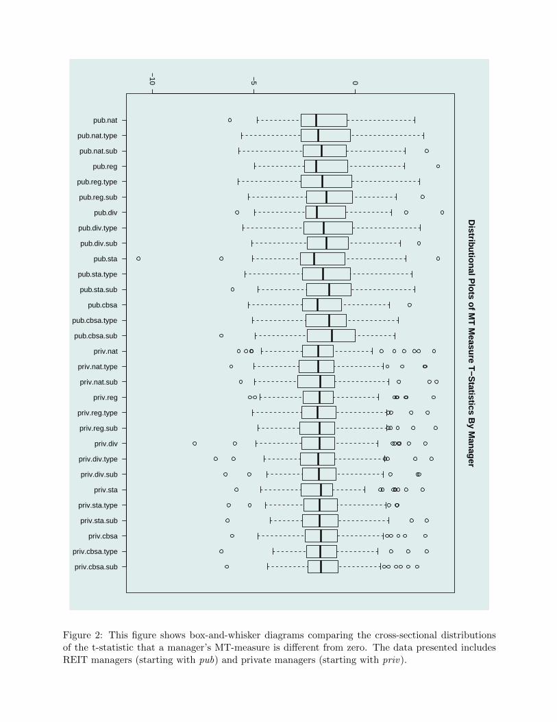
pub.nat

pub.nat.type

pub.nat.sub

pub.reg

pub.reg.type

pub.reg.sub

pub.div

pub.div.type

pub.div.sub

pub.sta

pub.sta.type

pub.sta.sub

pub.cbsa

pub.cbsa.type

pub.cbsa.sub

priv.nat

priv.nat.type

priv.nat.sub

priv.reg

priv.reg.type

priv.reg.sub

priv.div

priv.div.type

priv.div.sub

priv.sta

priv.sta.type

priv.sta.sub

priv.cbsa

priv.cbsa.type

priv.cbsa.sub

−10

−5 0

Distributional P

lots of MT

Measure T

−Statistics B

y Manager

Figure 2: This figure shows box-and-whisker diagrams comparing the cross-sectional distributionsof the t-statistic that a manager’s MT-measure is different from zero. The data presented includesREIT managers (starting with pub) and private managers (starting with priv).

pub.nat

pub.nat.type

pub.nat.sub

pub.reg

pub.reg.type

pub.reg.sub

pub.div

pub.div.type

pub.div.sub

pub.sta

pub.sta.type

pub.sta.sub

pub.cbsa

priv.nat

priv.nat.type

priv.nat.sub

priv.reg

priv.reg.type

priv.reg.sub

priv.div

priv.div.type

priv.div.sub

priv.sta

priv.sta.type

priv.sta.sub

priv.cbsa

−0.03

−0.02

−0.01

0.00

0.01

0.02

Distribu

tion

al Plo

ts of M

S M

easures B

y Man

ager

Figure 3: This figure shows box-and-whisker diagrams comparing the cross-sectional distributions ofMS measures obtained by managers with respect to the various aggregation levels of benchmarks.The data presented includes REIT managers (starting with pub) and private managers (starting withpriv).

pub.nat

pub.nat.type

pub.nat.sub

pub.reg

pub.reg.type

pub.reg.sub

pub.div

pub.div.type

pub.div.sub

pub.sta

pub.sta.type

pub.sta.sub

pub.cbsa

priv.nat

priv.nat.type

priv.nat.sub

priv.reg

priv.reg.type

priv.reg.sub

priv.div

priv.div.type

priv.div.sub

priv.sta

priv.sta.type

priv.sta.sub

priv.cbsa

−6

−4

−2 0 2 4 6

Distributional P

lots of MS

Measure T

−Statistics B

y Manager

Figure 4: This figure shows box-and-whisker diagrams comparing the cross-sectional distributionsof the t-statistic that a manager’s MS-measure is different from zero. The data presented includesREIT managers (starting with pub) and private managers (starting with priv).

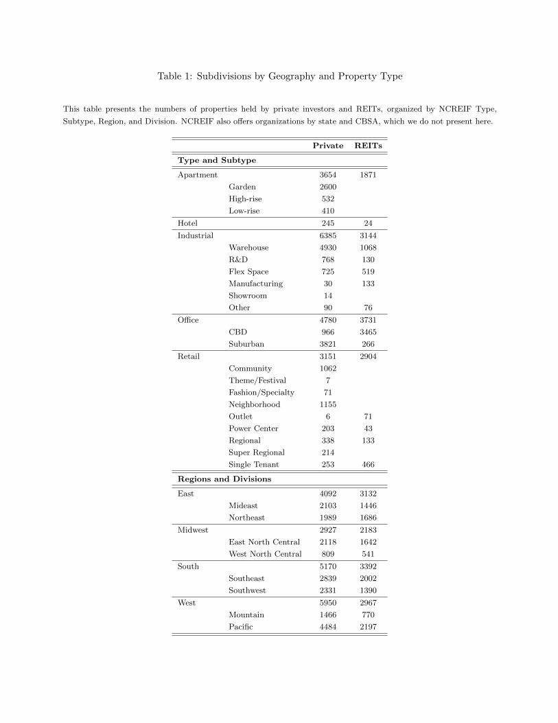
Table 1: Subdivisions by Geography and Property Type

This table presents the numbers of properties held by private investors and REITs, organized by NCREIF Type,

Subtype, Region, and Division. NCREIF also offers organizations by state and CBSA, which we do not present here.

Private REITs

Type and Subtype

Apartment 3654 1871

Garden 2600

High-rise 532

Low-rise 410

Hotel 245 24

Industrial 6385 3144

Warehouse 4930 1068

R&D 768 130

Flex Space 725 519

Manufacturing 30 133

Showroom 14

Other 90 76

Office 4780 3731

CBD 966 3465

Suburban 3821 266

Retail 3151 2904

Community 1062

Theme/Festival 7

Fashion/Specialty 71

Neighborhood 1155

Outlet 6 71

Power Center 203 43

Regional 338 133

Super Regional 214

Single Tenant 253 466

Regions and Divisions

East 4092 3132

Mideast 2103 1446

Northeast 1989 1686

Midwest 2927 2183

East North Central 2118 1642

West North Central 809 541

South 5170 3392

Southeast 2839 2002

Southwest 2331 1390

West 5950 2967

Mountain 1466 770

Pacific 4484 2197

Table 2: Summary Statistics

This table presents summary statistics for the sets of properties held by both private investors and Real Estate

Investment Trusts.

Mean Std. Dev. 1st Quartile Median 3rd Quartile

REITs

Property Sizes (1000 Sq. ft.) 182.63 235.44 52.87 114.87 228

Portfolio Sizes (1000 Sq. ft.) 21, 460.15 26, 077.87 6, 263.01 14, 386.73 24, 868.9

Portfolio Presence in Number of CBSAs 11.37 12.27 2.25 8 16

Number of Property Types in Portfolios 1.85 1.01 1 2 2

Number of Property Subtypes in Portfolios 2.93 2.1 1 2 4

Property Holding Periods (years) 6.03 4.88 2.68 4.87 8.21

Manager Number of Years in Sample 8.22 4.59 4 8 12.25

Manager HHI, by Region 0.72 0.25 0.5 0.71 1

Manager HHI, by Division 0.64 0.28 0.41 0.59 0.98

Manager HHI, by State 0.57 0.3 0.32 0.5 0.9

Manager HHI, by CBSA 0.5 0.31 0.24 0.4 0.79

Manager HHI, by Type 0.87 0.18 0.76 0.99 1

Manager HHI, by Subtype 0.78 0.23 0.6 0.84 1

Number of Properties: 11,674 Number of Managers: 210

Private Portfolios

Property Sizes (1000 Sq. ft.) 268.02 432 92.02 173.98 316.82

Portfolio Sizes (1000 Sq. ft.) 42, 060.43 44, 311.33 10, 917.88 29, 775.05 52, 475.24

Portfolio Presence in Number of CBSAs 30.94 28.15 10.75 22 41.25

Number of Property Types in Portfolios 3.35 1.3 3 4 4

Number of Property Subtypes in Portfolios 7.69 4.82 4 6 11

Property Holding Periods (years) 4.65 3.55 2.25 3.75 6.25

Manager Number of Years in Sample 10.84 8.29 3.75 9.25 15.38

Manager HHI, by Region 0.51 0.23 0.34 0.42 0.62

Manager HHI, by Division 0.41 0.24 0.23 0.32 0.51

Manager HHI, by State 0.33 0.24 0.15 0.25 0.41

Manager HHI, by CBSA 0.26 0.22 0.1 0.18 0.35

Manager HHI, by Type 0.62 0.23 0.45 0.57 0.8

Manager HHI, by Subtype 0.49 0.21 0.33 0.43 0.59

Number of Properties: 18,115 Number of Managers: 136

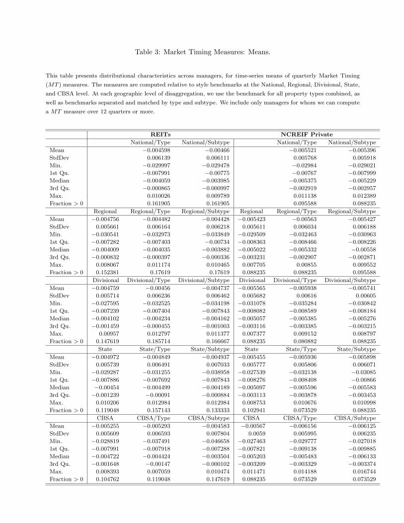
Table 3: Market Timing Measures: Means.

This table presents distributional characteristics across managers, for time-series means of quarterly Market Timing

(MT ) measures. The measures are computed relative to style benchmarks at the National, Regional, Divisional, State,

and CBSA level. At each geographic level of disaggregation, we use the benchmark for all property types combined, as

well as benchmarks separated and matched by type and subtype. We include only managers for whom we can compute

a MT measure over 12 quarters or more.

REITs NCREIF Private

National/Type National/Subtype National/Type National/Subtype

Mean −0.004598 −0.00466 −0.005521 −0.005396

StdDev 0.006139 0.006111 0.005768 0.005918

Min. −0.029997 −0.029478 −0.02984 −0.029021

1st Qu. −0.007991 −0.00775 −0.00767 −0.007999

Median −0.004059 −0.003985 −0.005375 −0.005229

3rd Qu. −0.000865 −0.000997 −0.002919 −0.002957

Max. 0.010026 0.009789 0.011138 0.012389

Fraction > 0 0.161905 0.161905 0.095588 0.088235

Regional Regional/Type Regional/Subtype Regional Regional/Type Regional/Subtype

Mean −0.004756 −0.004482 −0.004428 −0.005423 −0.00563 −0.005427

StdDev 0.005661 0.006164 0.006218 0.005611 0.006034 0.006188

Min. −0.030541 −0.032973 −0.033849 −0.029509 −0.032463 −0.030963

1st Qu. −0.007282 −0.007403 −0.00734 −0.008363 −0.008466 −0.008226

Median −0.004009 −0.004035 −0.003882 −0.005022 −0.005332 −0.00558

3rd Qu. −0.000832 −0.000397 −0.000336 −0.003231 −0.002907 −0.002871

Max. 0.008067 0.011174 0.010465 0.007705 0.00855 0.009552

Fraction > 0 0.152381 0.17619 0.17619 0.088235 0.088235 0.095588

Divisional Divisional/Type Divisional/Subtype Divisional Divisional/Type Divisional/Subtype

Mean −0.004759 −0.00456 −0.004737 −0.005565 −0.005938 −0.005741

StdDev 0.005714 0.006236 0.006462 0.005682 0.00616 0.00605

Min. −0.027595 −0.032525 −0.034198 −0.031078 −0.035284 −0.030842

1st Qu. −0.007239 −0.007404 −0.007843 −0.008082 −0.008589 −0.008184

Median −0.004102 −0.004234 −0.004162 −0.005057 −0.005385 −0.005276

3rd Qu. −0.001459 −0.000455 −0.001003 −0.003116 −0.003385 −0.003215

Max. 0.00957 0.012797 0.011377 0.007377 0.009152 0.008797

Fraction > 0 0.147619 0.185714 0.166667 0.088235 0.080882 0.088235

State State/Type State/Subtype State State/Type State/Subtype

Mean −0.004972 −0.004849 −0.004937 −0.005455 −0.005936 −0.005898

StdDev 0.005739 0.006491 0.007033 0.005777 0.005806 0.006071

Min. −0.029287 −0.031255 −0.038958 −0.027539 −0.032138 −0.03085

1st Qu. −0.007886 −0.007692 −0.007843 −0.008276 −0.008408 −0.00866

Median −0.00454 −0.004499 −0.004189 −0.005097 −0.005596 −0.005583

3rd Qu. −0.001239 −0.00091 −0.000884 −0.003113 −0.003878 −0.003453

Max. 0.010206 0.012984 0.012984 0.008753 0.010676 0.010998

Fraction > 0 0.119048 0.157143 0.133333 0.102941 0.073529 0.088235

CBSA CBSA/Type CBSA/Subtype CBSA CBSA/Type CBSA/Subtype

Mean −0.005255 −0.005293 −0.004583 −0.00567 −0.006156 −0.006125

StdDev 0.005609 0.006593 0.007804 0.0059 0.005995 0.006235

Min. −0.028819 −0.037491 −0.046658 −0.027463 −0.029777 −0.027018

1st Qu. −0.007991 −0.007918 −0.007288 −0.007821 −0.009138 −0.009885

Median −0.004722 −0.004424 −0.003504 −0.005203 −0.005483 −0.006133

3rd Qu. −0.001648 −0.00147 −0.000102 −0.003209 −0.003329 −0.003374

Max. 0.008393 0.007059 0.010474 0.011471 0.014188 0.016744

Fraction > 0 0.104762 0.119048 0.147619 0.088235 0.073529 0.073529

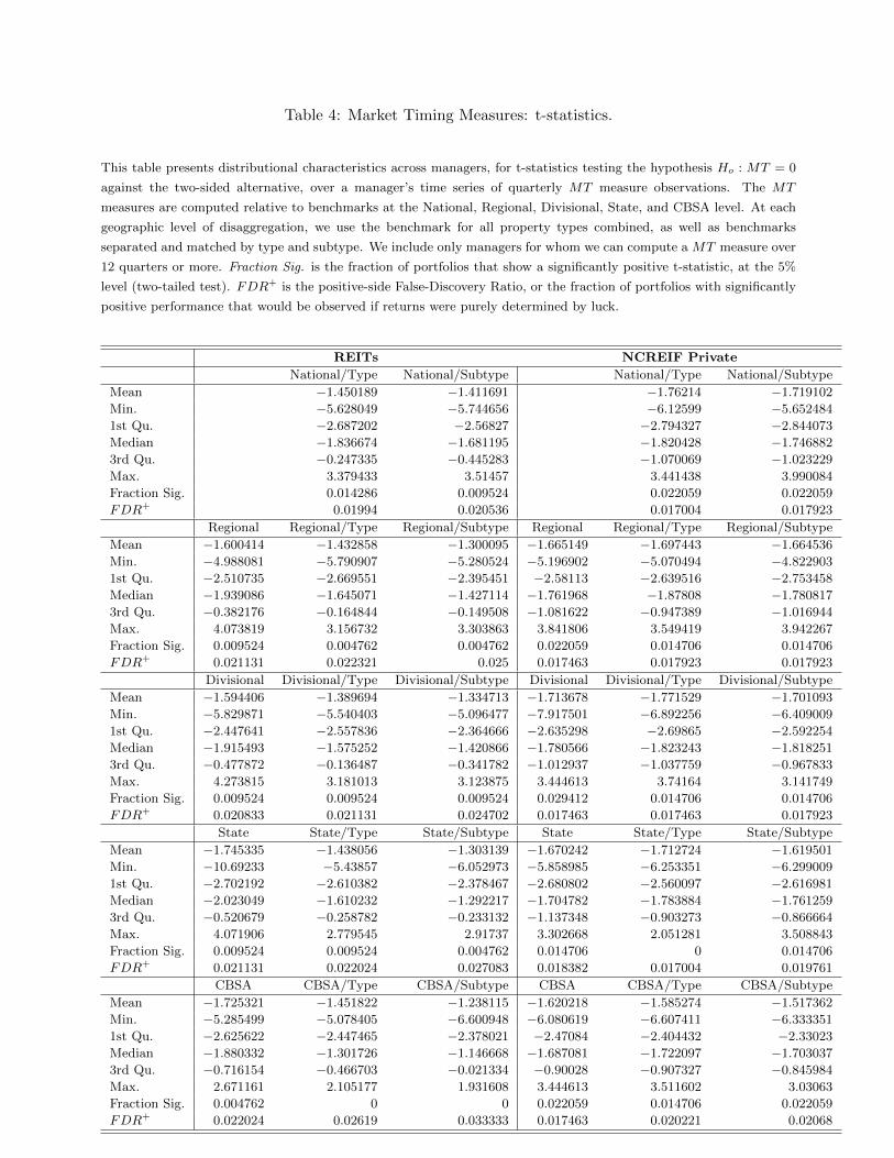
Table 4: Market Timing Measures: t-statistics.

This table presents distributional characteristics across managers, for t-statistics testing the hypothesis Ho : MT = 0

against the two-sided alternative, over a manager’s time series of quarterly MT measure observations. The MT

measures are computed relative to benchmarks at the National, Regional, Divisional, State, and CBSA level. At each

geographic level of disaggregation, we use the benchmark for all property types combined, as well as benchmarks

separated and matched by type and subtype. We include only managers for whom we can compute a MT measure over

12 quarters or more. Fraction Sig. is the fraction of portfolios that show a significantly positive t-statistic, at the 5%

level (two-tailed test). FDR+ is the positive-side False-Discovery Ratio, or the fraction of portfolios with significantly

positive performance that would be observed if returns were purely determined by luck.

REITs NCREIF Private

National/Type National/Subtype National/Type National/Subtype

Mean −1.450189 −1.411691 −1.76214 −1.719102

Min. −5.628049 −5.744656 −6.12599 −5.652484

1st Qu. −2.687202 −2.56827 −2.794327 −2.844073

Median −1.836674 −1.681195 −1.820428 −1.746882

3rd Qu. −0.247335 −0.445283 −1.070069 −1.023229

Max. 3.379433 3.51457 3.441438 3.990084

Fraction Sig. 0.014286 0.009524 0.022059 0.022059

FDR+ 0.01994 0.020536 0.017004 0.017923

Regional Regional/Type Regional/Subtype Regional Regional/Type Regional/Subtype

Mean −1.600414 −1.432858 −1.300095 −1.665149 −1.697443 −1.664536

Min. −4.988081 −5.790907 −5.280524 −5.196902 −5.070494 −4.822903

1st Qu. −2.510735 −2.669551 −2.395451 −2.58113 −2.639516 −2.753458

Median −1.939086 −1.645071 −1.427114 −1.761968 −1.87808 −1.780817

3rd Qu. −0.382176 −0.164844 −0.149508 −1.081622 −0.947389 −1.016944

Max. 4.073819 3.156732 3.303863 3.841806 3.549419 3.942267

Fraction Sig. 0.009524 0.004762 0.004762 0.022059 0.014706 0.014706

FDR+ 0.021131 0.022321 0.025 0.017463 0.017923 0.017923

Divisional Divisional/Type Divisional/Subtype Divisional Divisional/Type Divisional/Subtype

Mean −1.594406 −1.389694 −1.334713 −1.713678 −1.771529 −1.701093

Min. −5.829871 −5.540403 −5.096477 −7.917501 −6.892256 −6.409009

1st Qu. −2.447641 −2.557836 −2.364666 −2.635298 −2.69865 −2.592254

Median −1.915493 −1.575252 −1.420866 −1.780566 −1.823243 −1.818251

3rd Qu. −0.477872 −0.136487 −0.341782 −1.012937 −1.037759 −0.967833

Max. 4.273815 3.181013 3.123875 3.444613 3.74164 3.141749

Fraction Sig. 0.009524 0.009524 0.009524 0.029412 0.014706 0.014706

FDR+ 0.020833 0.021131 0.024702 0.017463 0.017463 0.017923

State State/Type State/Subtype State State/Type State/Subtype

Mean −1.745335 −1.438056 −1.303139 −1.670242 −1.712724 −1.619501

Min. −10.69233 −5.43857 −6.052973 −5.858985 −6.253351 −6.299009

1st Qu. −2.702192 −2.610382 −2.378467 −2.680802 −2.560097 −2.616981

Median −2.023049 −1.610232 −1.292217 −1.704782 −1.783884 −1.761259

3rd Qu. −0.520679 −0.258782 −0.233132 −1.137348 −0.903273 −0.866664

Max. 4.071906 2.779545 2.91737 3.302668 2.051281 3.508843

Fraction Sig. 0.009524 0.009524 0.004762 0.014706 0 0.014706

FDR+ 0.021131 0.022024 0.027083 0.018382 0.017004 0.019761

CBSA CBSA/Type CBSA/Subtype CBSA CBSA/Type CBSA/Subtype

Mean −1.725321 −1.451822 −1.238115 −1.620218 −1.585274 −1.517362

Min. −5.285499 −5.078405 −6.600948 −6.080619 −6.607411 −6.333351

1st Qu. −2.625622 −2.447465 −2.378021 −2.47084 −2.404432 −2.33023

Median −1.880332 −1.301726 −1.146668 −1.687081 −1.722097 −1.703037

3rd Qu. −0.716154 −0.466703 −0.021334 −0.90028 −0.907327 −0.845984

Max. 2.671161 2.105177 1.931608 3.444613 3.511602 3.03063

Fraction Sig. 0.004762 0 0 0.022059 0.014706 0.022059

FDR+ 0.022024 0.02619 0.033333 0.017463 0.020221 0.02068

Table 5: Market Selection Measures: Means.

This table presents distributional characteristics across managers, for time-series means of quarterly Market Selection

(MS) measures. The measures are computed relative to benchmarks at the National, Regional, Divisional, State, and

CBSA level. At each geographic level of disaggregation, we use the benchmark for all property types combined, as well

as benchmarks separated and matched by type and subtype. We include only managers for whom we can compute an

MS measure over 12 quarters or more.

REITs NCREIF Private

National National/Type National/Subtype National National/Type National/Subtype

Mean −0.00022 −0.000146 −0.000859 −0.000192 −0.000215 −0.000187

StdDev 0.004523 0.004013 0.004205 0.003532 0.002621 0.002439

Min. −0.019699 −0.015679 −0.019044 −0.013187 −0.009116 −0.008667

1st Qu. −0.002593 −0.002252 −0.003346 −0.001773 −0.001264 −0.001052

Median −5e− 04 −0.000472 −0.000887 −7.6e− 05 −0.000228 −8.2e− 05

3rd Qu. 0.002045 0.001788 0.001482 0.001681 0.001197 0.001089

Max. 0.020836 0.01626 0.015667 0.012988 0.00695 0.007643

Fraction > 0 0.366667 0.333333 0.3 0.397059 0.367647 0.382353

Regional Regional/Type Regional/Subtype Regional Regional/Type Regional/Subtype

Mean 0.000194 0.000192 −0.000444 8.4e− 05 7.1e− 05 9.4e− 05

StdDev 0.00443 0.003325 0.003654 0.003147 0.00212 0.002047

Min. −0.021777 −0.014922 −0.014332 −0.009163 −0.007357 −0.007432

1st Qu. −0.001591 −0.001379 −0.002004 −0.001415 −0.00073 −0.000688

Median −2.5e− 05 −9e− 06 −0.000375 0.000335 0.000155 0.00017

3rd Qu. 0.001972 0.001668 0.001166 0.001685 0.001152 0.001021

Max. 0.016648 0.013952 0.012119 0.011523 0.009032 0.008708

Fraction > 0 0.390476 0.395238 0.338095 0.477941 0.455882 0.433824

Divisional Divisional/Type Divisional/Subtype Divisional Divisional/Type Divisional/Subtype

Mean 0.000189 0.000229 −0.000432 4.8e− 05 −3.4e− 05 2.5e− 05

StdDev 0.004484 0.003143 0.003366 0.002934 0.001798 0.001822

Min. −0.022997 −0.016104 −0.015745 −0.009131 −0.007509 −0.007106

1st Qu. −0.001346 −0.000908 −0.001638 −0.00116 −0.000672 −0.000575

Median 0.000176 0.000204 −0.000206 9.1e− 05 3.4e− 05 5.9e− 05

3rd Qu. 0.001503 0.001534 0.001055 0.001343 0.000758 0.000776

Max. 0.016489 0.013453 0.012204 0.011177 0.007313 0.007319

Fraction > 0 0.428571 0.438095 0.352381 0.426471 0.426471 0.411765

State State/Type State/Subtype State State/Type State/Subtype

Mean 0.000156 0.000308 −5.1e− 05 7.6e− 05 0.00018 0.000163

StdDev 0.004344 0.00253 0.002505 0.002897 0.001566 0.001622

Min. −0.023742 −0.015998 −0.015572 −0.008915 −0.007159 −0.00643

1st Qu. −0.001256 −0.000328 −0.000533 −0.000994 −0.000455 −0.000561

Median 0.000126 0.00023 2.5e− 05 0.000315 2.3e− 05 −2.3e− 05

3rd Qu. 0.00142 0.001008 0.000807 0.001114 0.000599 0.00065

Max. 0.016086 0.012239 0.011195 0.01031 0.007938 0.007784

Fraction > 0 0.442857 0.471429 0.37619 0.463235 0.419118 0.389706

CBSA CBSA

Mean 3.1e− 05 3.6e− 05

StdDev 0.003996 0.002412

Min. −0.028883 −0.008159

1st Qu. −0.00131 −0.000728

Median 0.000153 8.3e− 05

3rd Qu. 0.001405 0.000955

Max. 0.01266 0.009639

Fraction > 0 0.42381 0.433824

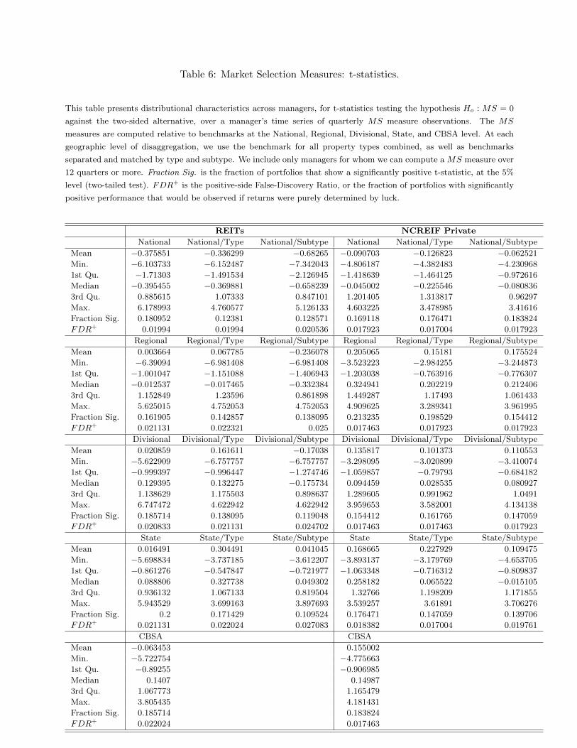
Table 6: Market Selection Measures: t-statistics.

This table presents distributional characteristics across managers, for t-statistics testing the hypothesis Ho : MS = 0

against the two-sided alternative, over a manager’s time series of quarterly MS measure observations. The MS

measures are computed relative to benchmarks at the National, Regional, Divisional, State, and CBSA level. At each

geographic level of disaggregation, we use the benchmark for all property types combined, as well as benchmarks

separated and matched by type and subtype. We include only managers for whom we can compute a MS measure over

12 quarters or more. Fraction Sig. is the fraction of portfolios that show a significantly positive t-statistic, at the 5%

level (two-tailed test). FDR+ is the positive-side False-Discovery Ratio, or the fraction of portfolios with significantly

positive performance that would be observed if returns were purely determined by luck.

REITs NCREIF Private

National National/Type National/Subtype National National/Type National/Subtype

Mean −0.375851 −0.336299 −0.68265 −0.090703 −0.126823 −0.062521

Min. −6.103733 −6.152487 −7.342043 −4.806187 −4.382483 −4.230968

1st Qu. −1.71303 −1.491534 −2.126945 −1.418639 −1.464125 −0.972616

Median −0.395455 −0.369881 −0.658239 −0.045002 −0.225546 −0.080836

3rd Qu. 0.885615 1.07333 0.847101 1.201405 1.313817 0.96297

Max. 6.178993 4.760577 5.126133 4.603225 3.478985 3.41616

Fraction Sig. 0.180952 0.12381 0.128571 0.169118 0.176471 0.183824

FDR+ 0.01994 0.01994 0.020536 0.017923 0.017004 0.017923

Regional Regional/Type Regional/Subtype Regional Regional/Type Regional/Subtype

Mean 0.003664 0.067785 −0.236078 0.205065 0.15181 0.175524

Min. −6.39094 −6.981408 −6.981408 −3.523223 −2.984255 −3.244873

1st Qu. −1.001047 −1.151088 −1.406943 −1.203038 −0.763916 −0.776307

Median −0.012537 −0.017465 −0.332384 0.324941 0.202219 0.212406

3rd Qu. 1.152849 1.23596 0.861898 1.449287 1.17493 1.061433

Max. 5.625015 4.752053 4.752053 4.909625 3.289341 3.961995

Fraction Sig. 0.161905 0.142857 0.138095 0.213235 0.198529 0.154412

FDR+ 0.021131 0.022321 0.025 0.017463 0.017923 0.017923

Divisional Divisional/Type Divisional/Subtype Divisional Divisional/Type Divisional/Subtype

Mean 0.020859 0.161611 −0.17038 0.135817 0.101373 0.110553

Min. −5.622909 −6.757757 −6.757757 −3.298095 −3.020899 −3.410074

1st Qu. −0.999397 −0.996447 −1.274746 −1.059857 −0.79793 −0.684182

Median 0.129395 0.132275 −0.175734 0.094459 0.028535 0.080927

3rd Qu. 1.138629 1.175503 0.898637 1.289605 0.991962 1.0491

Max. 6.747472 4.622942 4.622942 3.959653 3.582001 4.134138

Fraction Sig. 0.185714 0.138095 0.119048 0.154412 0.161765 0.147059

FDR+ 0.020833 0.021131 0.024702 0.017463 0.017463 0.017923

State State/Type State/Subtype State State/Type State/Subtype

Mean 0.016491 0.304491 0.041045 0.168665 0.227929 0.109475

Min. −5.698834 −3.737185 −3.612207 −3.893137 −3.179769 −4.653705

1st Qu. −0.861276 −0.547847 −0.721977 −1.063348 −0.716312 −0.809837

Median 0.088806 0.327738 0.049302 0.258182 0.065522 −0.015105

3rd Qu. 0.936132 1.067133 0.819504 1.32766 1.198209 1.171855

Max. 5.943529 3.699163 3.897693 3.539257 3.61891 3.706276

Fraction Sig. 0.2 0.171429 0.109524 0.176471 0.147059 0.139706

FDR+ 0.021131 0.022024 0.027083 0.018382 0.017004 0.019761

CBSA CBSA

Mean −0.063453 0.155002

Min. −5.722754 −4.775663

1st Qu. −0.89255 −0.906985

Median 0.1407 0.14987

3rd Qu. 1.067773 1.165479

Max. 3.805435 4.181431

Fraction Sig. 0.185714 0.183824

FDR+ 0.022024 0.017463

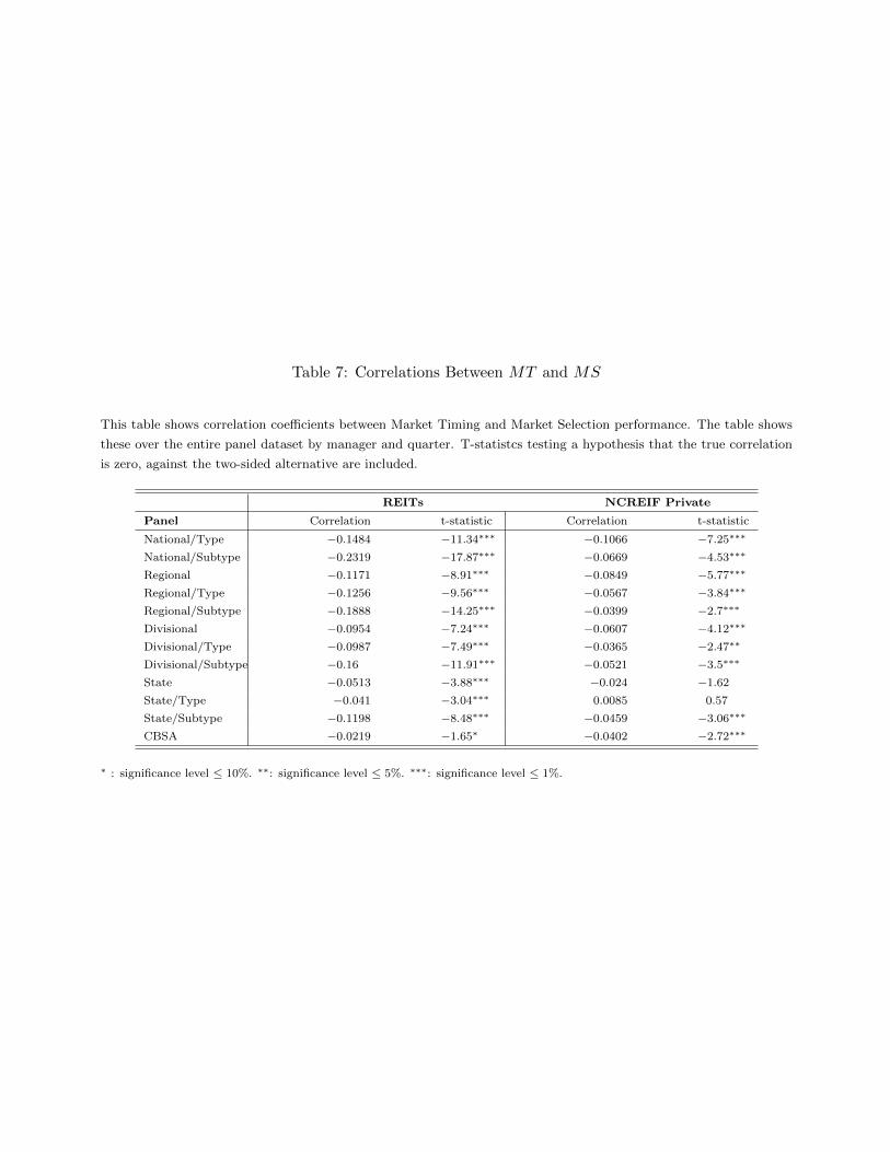
Table 7: Correlations Between MT and MS

This table shows correlation coefficients between Market Timing and Market Selection performance. The table shows

these over the entire panel dataset by manager and quarter. T-statistcs testing a hypothesis that the true correlation

is zero, against the two-sided alternative are included.

REITs NCREIF Private

Panel Correlation t-statistic Correlation t-statistic

National/Type −0.1484 −11.34∗∗∗ −0.1066 −7.25∗∗∗

National/Subtype −0.2319 −17.87∗∗∗ −0.0669 −4.53∗∗∗

Regional −0.1171 −8.91∗∗∗ −0.0849 −5.77∗∗∗

Regional/Type −0.1256 −9.56∗∗∗ −0.0567 −3.84∗∗∗

Regional/Subtype −0.1888 −14.25∗∗∗ −0.0399 −2.7∗∗∗

Divisional −0.0954 −7.24∗∗∗ −0.0607 −4.12∗∗∗

Divisional/Type −0.0987 −7.49∗∗∗ −0.0365 −2.47∗∗

Divisional/Subtype −0.16 −11.91∗∗∗ −0.0521 −3.5∗∗∗

State −0.0513 −3.88∗∗∗ −0.024 −1.62

State/Type −0.041 −3.04∗∗∗ 0.0085 0.57

State/Subtype −0.1198 −8.48∗∗∗ −0.0459 −3.06∗∗∗

CBSA −0.0219 −1.65∗ −0.0402 −2.72∗∗∗

∗ : significance level ≤ 10%. ∗∗: significance level ≤ 5%. ∗∗∗: significance level ≤ 1%.

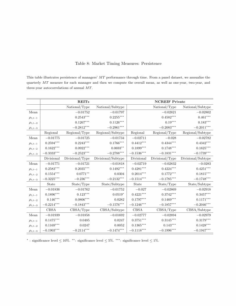
Table 8: Market Timing Measures: Persistence

This table illustrates persistence of managers’ MT performance through time. From a panel dataset, we annualize the

quarterly MT measure for each manager and then we compute the overall mean, as well as one-year, two-year, and

three-year autocorrelations of annual MT .

REITs NCREIF Private

National/Type National/Subtype National/Type National/Subtype

Mean −0.01752 −0.01797 −0.02821 −0.02802

ρt,t−1 0.2543∗∗∗ 0.2255∗∗∗ 0.4582∗∗∗ 0.461∗∗∗

ρt,t−2 0.1267∗∗∗ 0.1126∗∗∗ 0.19∗∗∗ 0.183∗∗∗

ρt,t−3 −0.2812∗∗∗ −0.2961∗∗∗ −0.2083∗∗∗ −0.2011∗∗∗

Regional Regional/Type Regional/Subtype Regional Regional/Type Regional/Subtype

Mean −0.01775 −0.01725 −0.01734 −0.02711 −0.028 −0.02782

ρt,t−1 0.2594∗∗∗ 0.2243∗∗∗ 0.1766∗∗∗ 0.4412∗∗∗ 0.4344∗∗∗ 0.4342∗∗∗

ρt,t−2 0.1622∗∗∗ 0.0922∗∗∗ 0.0693∗∗ 0.1899∗∗∗ 0.1748∗∗∗ 0.1625∗∗∗

ρt,t−3 −0.3333∗∗∗ −0.2523∗∗∗ −0.2788∗∗∗ −0.1536∗∗∗ −0.1831∗∗∗ −0.1739∗∗∗

Divisional Divisional/Type Divisional/Subtype Divisional Divisional/Type Divisional/Subtype

Mean −0.01771 −0.01721 −0.01818 −0.02719 −0.02832 −0.0283

ρt,t−1 0.2583∗∗∗ 0.2035∗∗∗ 0.1492∗∗∗ 0.4281∗∗∗ 0.4224∗∗∗ 0.4251∗∗∗

ρt,t−2 0.1554∗∗∗ 0.0771∗∗ 0.0304 0.2014∗∗∗ 0.1772∗∗∗ 0.1815∗∗∗

ρt,t−3 −0.3225∗∗∗ −0.236∗∗∗ −0.2132∗∗∗ −0.1514∗∗∗ −0.1785∗∗∗ −0.1748∗∗∗

State State/Type State/Subtype State State/Type State/Subtype

Mean −0.01836 −0.01762 −0.01752 −0.027 −0.02869 −0.02918

ρt,t−1 0.1896∗∗∗ 0.123∗∗∗ 0.0519∗ 0.4221∗∗∗ 0.3742∗∗∗ 0.3457∗∗∗

ρt,t−2 0.146∗∗∗ 0.0806∗∗∗ 0.0282 0.1797∗∗∗ 0.1469∗∗∗ 0.1171∗∗∗

ρt,t−3 −0.2214∗∗∗ −0.1843∗∗∗ −0.1576∗∗∗ −0.1246∗∗∗ −0.1857∗∗∗ −0.2046∗∗∗

CBSA CBSA/Type CBSA/Subtype CBSA CBSA/Type CBSA/Subtype

Mean −0.01939 −0.01858 −0.01692 −0.02777 −0.02894 −0.02979

ρt,t−1 0.1475∗∗∗ 0.0485 0.0247 0.3751∗∗∗ 0.3145∗∗∗ 0.3179∗∗∗

ρt,t−2 0.1169∗∗∗ 0.0247 0.0052 0.1365∗∗∗ 0.143∗∗∗ 0.1428∗∗∗

ρt,t−3 −0.1903∗∗∗ −0.2114∗∗∗ −0.1474∗∗∗ −0.1118∗∗∗ −0.1996∗∗∗ −0.1947∗∗∗

∗ : significance level ≤ 10%. ∗∗: significance level ≤ 5%. ∗∗∗: significance level ≤ 1%.

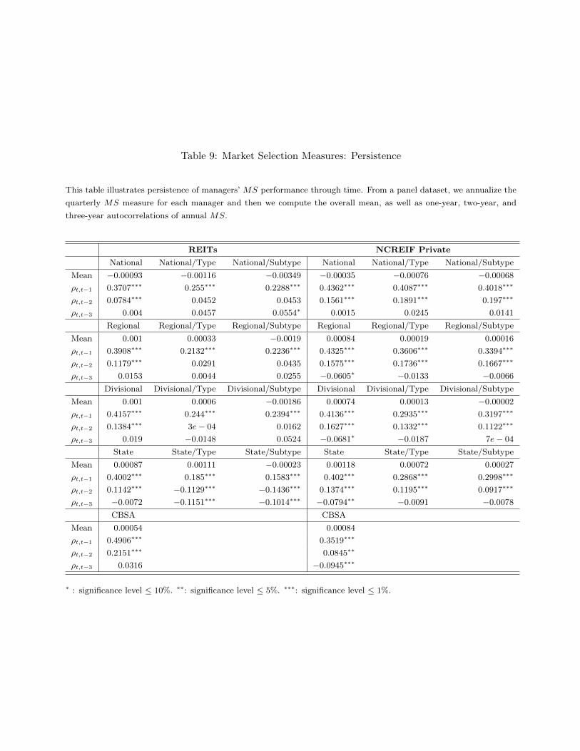
Table 9: Market Selection Measures: Persistence

This table illustrates persistence of managers’ MS performance through time. From a panel dataset, we annualize the

quarterly MS measure for each manager and then we compute the overall mean, as well as one-year, two-year, and

three-year autocorrelations of annual MS.

REITs NCREIF Private

National National/Type National/Subtype National National/Type National/Subtype

Mean −0.00093 −0.00116 −0.00349 −0.00035 −0.00076 −0.00068

ρt,t−1 0.3707∗∗∗ 0.255∗∗∗ 0.2288∗∗∗ 0.4362∗∗∗ 0.4087∗∗∗ 0.4018∗∗∗

ρt,t−2 0.0784∗∗∗ 0.0452 0.0453 0.1561∗∗∗ 0.1891∗∗∗ 0.197∗∗∗

ρt,t−3 0.004 0.0457 0.0554∗ 0.0015 0.0245 0.0141

Regional Regional/Type Regional/Subtype Regional Regional/Type Regional/Subtype

Mean 0.001 0.00033 −0.0019 0.00084 0.00019 0.00016

ρt,t−1 0.3908∗∗∗ 0.2132∗∗∗ 0.2236∗∗∗ 0.4325∗∗∗ 0.3606∗∗∗ 0.3394∗∗∗

ρt,t−2 0.1179∗∗∗ 0.0291 0.0435 0.1575∗∗∗ 0.1736∗∗∗ 0.1667∗∗∗

ρt,t−3 0.0153 0.0044 0.0255 −0.0605∗ −0.0133 −0.0066

Divisional Divisional/Type Divisional/Subtype Divisional Divisional/Type Divisional/Subtype

Mean 0.001 0.0006 −0.00186 0.00074 0.00013 −0.00002

ρt,t−1 0.4157∗∗∗ 0.244∗∗∗ 0.2394∗∗∗ 0.4136∗∗∗ 0.2935∗∗∗ 0.3197∗∗∗

ρt,t−2 0.1384∗∗∗ 3e− 04 0.0162 0.1627∗∗∗ 0.1332∗∗∗ 0.1122∗∗∗

ρt,t−3 0.019 −0.0148 0.0524 −0.0681∗ −0.0187 7e− 04

State State/Type State/Subtype State State/Type State/Subtype

Mean 0.00087 0.00111 −0.00023 0.00118 0.00072 0.00027

ρt,t−1 0.4002∗∗∗ 0.185∗∗∗ 0.1583∗∗∗ 0.402∗∗∗ 0.2868∗∗∗ 0.2998∗∗∗

ρt,t−2 0.1142∗∗∗ −0.1129∗∗∗ −0.1436∗∗∗ 0.1374∗∗∗ 0.1195∗∗∗ 0.0917∗∗∗

ρt,t−3 −0.0072 −0.1151∗∗∗ −0.1014∗∗∗ −0.0794∗∗ −0.0091 −0.0078

CBSA CBSA

Mean 0.00054 0.00084

ρt,t−1 0.4906∗∗∗ 0.3519∗∗∗

ρt,t−2 0.2151∗∗∗ 0.0845∗∗

ρt,t−3 0.0316 −0.0945∗∗∗

∗ : significance level ≤ 10%. ∗∗: significance level ≤ 5%. ∗∗∗: significance level ≤ 1%.

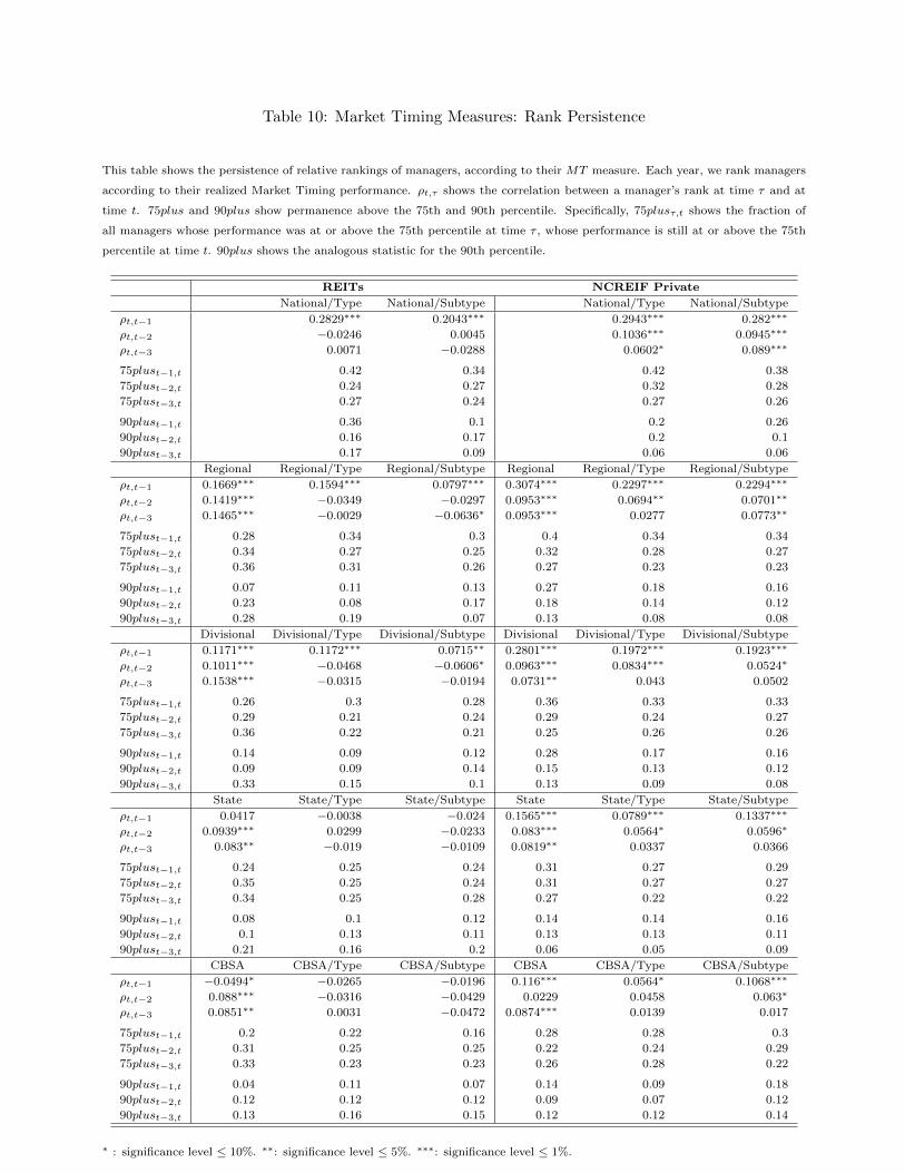
Table 10: Market Timing Measures: Rank Persistence

This table shows the persistence of relative rankings of managers, according to their MT measure. Each year, we rank managers

according to their realized Market Timing performance. ρt,τ shows the correlation between a manager’s rank at time τ and at

time t. 75plus and 90plus show permanence above the 75th and 90th percentile. Specifically, 75plusτ,t shows the fraction of

all managers whose performance was at or above the 75th percentile at time τ , whose performance is still at or above the 75th

percentile at time t. 90plus shows the analogous statistic for the 90th percentile.

REITs NCREIF Private

National/Type National/Subtype National/Type National/Subtype

ρt,t−1 0.2829∗∗∗ 0.2043∗∗∗ 0.2943∗∗∗ 0.282∗∗∗

ρt,t−2 −0.0246 0.0045 0.1036∗∗∗ 0.0945∗∗∗

ρt,t−3 0.0071 −0.0288 0.0602∗ 0.089∗∗∗

75plust−1,t 0.42 0.34 0.42 0.38

75plust−2,t 0.24 0.27 0.32 0.28

75plust−3,t 0.27 0.24 0.27 0.26

90plust−1,t 0.36 0.1 0.2 0.26

90plust−2,t 0.16 0.17 0.2 0.1

90plust−3,t 0.17 0.09 0.06 0.06

Regional Regional/Type Regional/Subtype Regional Regional/Type Regional/Subtype

ρt,t−1 0.1669∗∗∗ 0.1594∗∗∗ 0.0797∗∗∗ 0.3074∗∗∗ 0.2297∗∗∗ 0.2294∗∗∗

ρt,t−2 0.1419∗∗∗ −0.0349 −0.0297 0.0953∗∗∗ 0.0694∗∗ 0.0701∗∗

ρt,t−3 0.1465∗∗∗ −0.0029 −0.0636∗ 0.0953∗∗∗ 0.0277 0.0773∗∗

75plust−1,t 0.28 0.34 0.3 0.4 0.34 0.34

75plust−2,t 0.34 0.27 0.25 0.32 0.28 0.27

75plust−3,t 0.36 0.31 0.26 0.27 0.23 0.23

90plust−1,t 0.07 0.11 0.13 0.27 0.18 0.16

90plust−2,t 0.23 0.08 0.17 0.18 0.14 0.12

90plust−3,t 0.28 0.19 0.07 0.13 0.08 0.08

Divisional Divisional/Type Divisional/Subtype Divisional Divisional/Type Divisional/Subtype

ρt,t−1 0.1171∗∗∗ 0.1172∗∗∗ 0.0715∗∗ 0.2801∗∗∗ 0.1972∗∗∗ 0.1923∗∗∗

ρt,t−2 0.1011∗∗∗ −0.0468 −0.0606∗ 0.0963∗∗∗ 0.0834∗∗∗ 0.0524∗

ρt,t−3 0.1538∗∗∗ −0.0315 −0.0194 0.0731∗∗ 0.043 0.0502

75plust−1,t 0.26 0.3 0.28 0.36 0.33 0.33

75plust−2,t 0.29 0.21 0.24 0.29 0.24 0.27

75plust−3,t 0.36 0.22 0.21 0.25 0.26 0.26

90plust−1,t 0.14 0.09 0.12 0.28 0.17 0.16

90plust−2,t 0.09 0.09 0.14 0.15 0.13 0.12

90plust−3,t 0.33 0.15 0.1 0.13 0.09 0.08

State State/Type State/Subtype State State/Type State/Subtype

ρt,t−1 0.0417 −0.0038 −0.024 0.1565∗∗∗ 0.0789∗∗∗ 0.1337∗∗∗

ρt,t−2 0.0939∗∗∗ 0.0299 −0.0233 0.083∗∗∗ 0.0564∗ 0.0596∗

ρt,t−3 0.083∗∗ −0.019 −0.0109 0.0819∗∗ 0.0337 0.0366

75plust−1,t 0.24 0.25 0.24 0.31 0.27 0.29

75plust−2,t 0.35 0.25 0.24 0.31 0.27 0.27

75plust−3,t 0.34 0.25 0.28 0.27 0.22 0.22

90plust−1,t 0.08 0.1 0.12 0.14 0.14 0.16

90plust−2,t 0.1 0.13 0.11 0.13 0.13 0.11

90plust−3,t 0.21 0.16 0.2 0.06 0.05 0.09

CBSA CBSA/Type CBSA/Subtype CBSA CBSA/Type CBSA/Subtype

ρt,t−1 −0.0494∗ −0.0265 −0.0196 0.116∗∗∗ 0.0564∗ 0.1068∗∗∗

ρt,t−2 0.088∗∗∗ −0.0316 −0.0429 0.0229 0.0458 0.063∗

ρt,t−3 0.0851∗∗ 0.0031 −0.0472 0.0874∗∗∗ 0.0139 0.017

75plust−1,t 0.2 0.22 0.16 0.28 0.28 0.3

75plust−2,t 0.31 0.25 0.25 0.22 0.24 0.29

75plust−3,t 0.33 0.23 0.23 0.26 0.28 0.22

90plust−1,t 0.04 0.11 0.07 0.14 0.09 0.18

90plust−2,t 0.12 0.12 0.12 0.09 0.07 0.12

90plust−3,t 0.13 0.16 0.15 0.12 0.12 0.14

∗ : significance level ≤ 10%. ∗∗: significance level ≤ 5%. ∗∗∗: significance level ≤ 1%.

Table 11: Market Selection Measures: Rank Persistence

This table shows the persistence of relative rankings of managers, according to their MS measure. Each year, we rank

managers according to their realized Market Selection performance. ρt,τ shows the correlation between a manager’s

rank at time τ and at time t. 75plus and 90plus show permanence above the 75th and 90th percentile. Specifically,

75plusτ,t shows the fraction of all managers whose performance was at or above the 75th percentile at time τ , whose

performance is still at or above the 75th percentile at time t. 90plus shows the analogous statistic for the 90th

percentile.

REITs NCREIF Private

National National/Type National/Subtype National National/Type National/Subtype

ρt,t−1 0.4324∗∗∗ 0.3736∗∗∗ 0.3609∗∗∗ 0.4499∗∗∗ 0.4101∗∗∗ 0.3703∗∗∗

ρt,t−2 0.1927∗∗∗ 0.2254∗∗∗ 0.241∗∗∗ 0.2264∗∗∗ 0.2295∗∗∗ 0.2324∗∗∗

ρt,t−3 0.0506 0.1624∗∗∗ 0.1705∗∗∗ 0.0949∗∗∗ 0.1135∗∗∗ 0.074∗∗

75plust−1,t 0.5 0.45 0.44 0.46 0.44 0.38

75plust−2,t 0.34 0.38 0.41 0.38 0.33 0.35

75plust−3,t 0.28 0.32 0.37 0.31 0.26 0.27

90plust−1,t 0.3 0.26 0.27 0.31 0.23 0.23

90plust−2,t 0.21 0.21 0.25 0.16 0.19 0.14

90plust−3,t 0.2 0.17 0.18 0.06 0.12 0.12

Regional Regional/Type Regional/Subtype Regional Regional/Type Regional/Subtype

ρt,t−1 0.3873∗∗∗ 0.2666∗∗∗ 0.2623∗∗∗ 0.3934∗∗∗ 0.329∗∗∗ 0.3075∗∗∗

ρt,t−2 0.1806∗∗∗ 0.1138∗∗∗ 0.1287∗∗∗ 0.1874∗∗∗ 0.1739∗∗∗ 0.1947∗∗∗

ρt,t−3 0.0376 0.0484 0.0446 0.04 0.0839∗∗ 0.0547

75plust−1,t 0.49 0.4 0.41 0.44 0.42 0.4

75plust−2,t 0.29 0.33 0.32 0.36 0.34 0.33

75plust−3,t 0.24 0.26 0.26 0.3 0.3 0.28

90plust−1,t 0.33 0.22 0.26 0.34 0.28 0.19

90plust−2,t 0.2 0.18 0.21 0.23 0.22 0.18

90plust−3,t 0.22 0.21 0.14 0.03 0.13 0.07

Divisional Divisional/Type Divisional/Subtype Divisional Divisional/Type Divisional/Subtype

ρt,t−1 0.3843∗∗∗ 0.2746∗∗∗ 0.2358∗∗∗ 0.3468∗∗∗ 0.2732∗∗∗ 0.306∗∗∗

ρt,t−2 0.166∗∗∗ 0.0965∗∗∗ 0.1072∗∗∗ 0.1788∗∗∗ 0.1515∗∗∗ 0.1414∗∗∗

ρt,t−3 0.0091 −0.0057 0.0339 0.0231 0.0833∗∗ 0.0364

75plust−1,t 0.5 0.42 0.38 0.45 0.4 0.38

75plust−2,t 0.32 0.32 0.3 0.38 0.32 0.3

75plust−3,t 0.24 0.26 0.25 0.28 0.29 0.26

90plust−1,t 0.39 0.26 0.31 0.34 0.26 0.25

90plust−2,t 0.19 0.22 0.15 0.21 0.18 0.18

90plust−3,t 0.2 0.19 0.13 0.07 0.1 0.12

State State/Type State/Subtype State State/Type State/Subtype

ρt,t−1 0.359∗∗∗ 0.1909∗∗∗ 0.1609∗∗∗ 0.3295∗∗∗ 0.2752∗∗∗ 0.2891∗∗∗

ρt,t−2 0.1179∗∗∗ 0.0431 −0.0165 0.1501∗∗∗ 0.1187∗∗∗ 0.1036∗∗∗

ρt,t−3 −0.0328 −0.0942∗∗∗ −0.0843∗∗ −0.018 0.0656∗ 0.0013

75plust−1,t 0.45 0.38 0.34 0.46 0.44 0.42

75plust−2,t 0.3 0.31 0.24 0.34 0.31 0.32

75plust−3,t 0.22 0.24 0.24 0.28 0.26 0.27

90plust−1,t 0.33 0.27 0.28 0.27 0.39 0.31

90plust−2,t 0.19 0.11 0.15 0.19 0.23 0.22

90plust−3,t 0.19 0.08 0.11 0.1 0.11 0.15

CBSA CBSA

ρt,t−1 0.4066∗∗∗ 0.2805∗∗∗

ρt,t−2 0.1336∗∗∗ 0.0741∗∗

ρt,t−3 −0.0528 −0.037

75plust−1,t 0.5 0.38

75plust−2,t 0.32 0.33

75plust−3,t 0.23 0.26

90plust−1,t 0.34 0.22

90plust−2,t 0.19 0.15

90plust−3,t 0.14 0.06

∗ : significance level ≤ 10%. ∗∗: significance level ≤ 5%. ∗∗∗: significance level ≤ 1%.

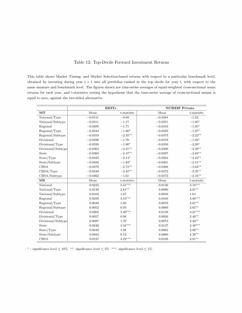
Table 12: Top-Decile Forward Investment Returns

This table shows Market Timing- and Market Selection-based returns with respect to a particular benchmark level,

obtained by investing during year t + 1 into all portfolios ranked in the top decile for year t, with respect to the

same measure and benchmark level. The figures shown are time-series averages of equal-weighted cross-sectional mean

returns for each year, and t-statistics testing the hypothesis that the time-series average of cross-sectional means is

equal to zero, against the two-sided alternative.

REITs NCREIF Private

MT Mean t-statistic Mean t-statistic

National/Type −0.0151 −0.69 −0.0284 −1.62

National/Subtype −0.0211 −1.17 −0.0331 −1.95∗

Regional −0.0299 −1.75 −0.0316 −1.95∗

Regional/Type −0.0344 −1.80∗ −0.0335 −1.97∗

Regional/Subtype −0.0359 −2.35∗∗ −0.0373 −2.22∗∗

Divisional −0.0296 −1.70 −0.0319 −1.94∗

Divisional/Type −0.0328 −1.90∗ −0.0350 −2.09∗

Divisional/Subtype −0.0364 −2.21∗∗ −0.0399 −2.29∗∗

State −0.0368 −2.47∗∗ −0.0397 −2.69∗∗

State/Type −0.0423 −2.14∗ −0.0384 −2.22∗∗

State/Subtype −0.0480 −1.94∗ −0.0401 −2.51∗∗

CBSA −0.0470 −2.72∗∗ −0.0408 −3.03∗∗

CBSA/Type −0.0530 −2.45∗∗ −0.0372 −2.35∗∗

CBSA/Subtype −0.0462 −1.61 −0.0373 −2.44∗∗

MS Mean t-statistic Mean t-statistic

National 0.0224 3.41∗∗∗ 0.0130 3.16∗∗∗

National/Type 0.0139 2.81∗∗ 0.0080 2.91∗∗

National/Subtype 0.0102 1.67 0.0046 1.64

Regional 0.0259 3.43∗∗∗ 0.0169 3.90∗∗∗

Regional/Type 0.0049 1.02 0.0078 2.61∗∗

Regional/Subtype 0.0052 0.93 0.0069 2.65∗∗

Divisional 0.0262 3.39∗∗∗ 0.0139 3.21∗∗∗

Divisional/Type 0.0057 0.98 0.0056 2.40∗∗

Divisional/Subtype 0.0087 1.70 0.0073 2.46∗∗

State 0.0240 3.34∗∗∗ 0.0137 3.49∗∗∗

State/Type 0.0049 1.08 0.0063 2.88∗∗

State/Subtype 0.0024 0.52 0.0060 2.39∗∗

CBSA 0.0197 3.22∗∗∗ 0.0108 2.81∗∗

∗ : significance level ≤ 10%. ∗∗: significance level ≤ 5%. ∗∗∗: significance level ≤ 1%.

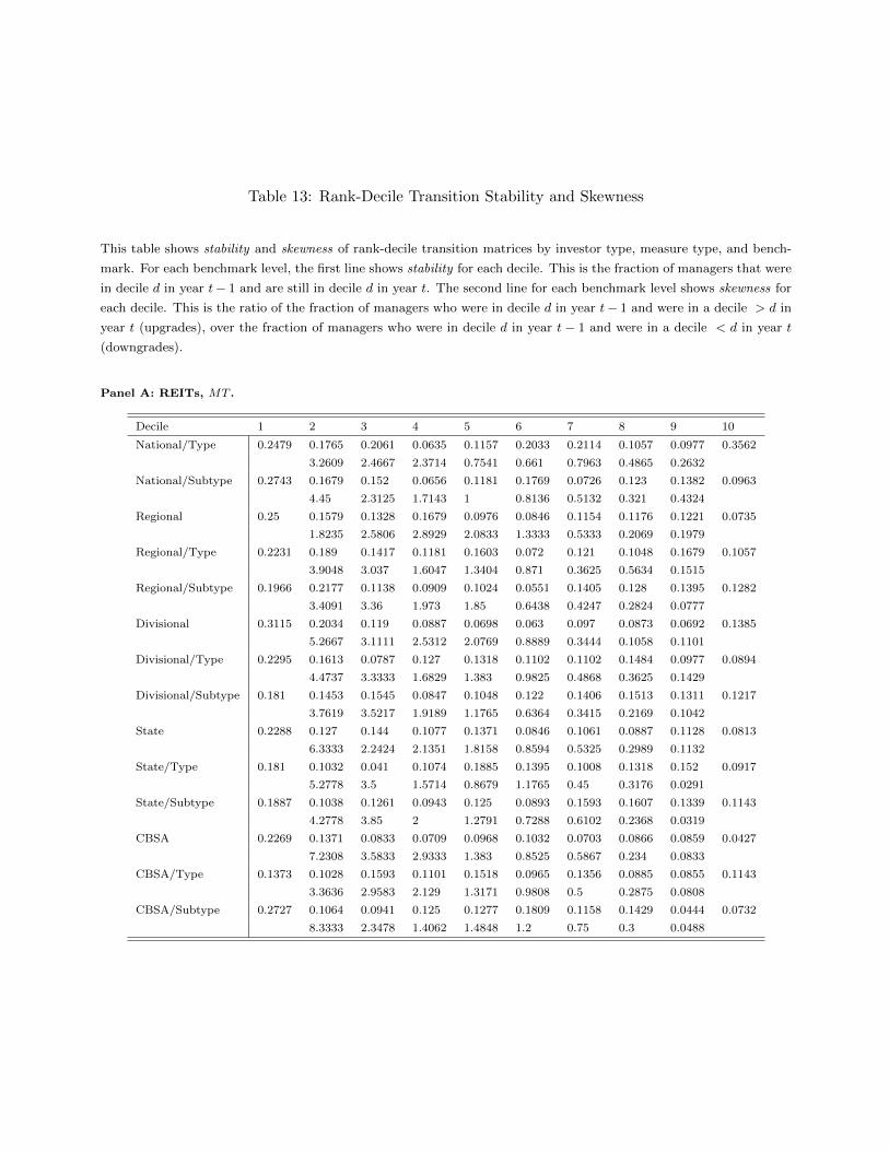
Table 13: Rank-Decile Transition Stability and Skewness

This table shows stability and skewness of rank-decile transition matrices by investor type, measure type, and bench-

mark. For each benchmark level, the first line shows stability for each decile. This is the fraction of managers that were

in decile d in year t− 1 and are still in decile d in year t. The second line for each benchmark level shows skewness for

each decile. This is the ratio of the fraction of managers who were in decile d in year t− 1 and were in a decile > d in

year t (upgrades), over the fraction of managers who were in decile d in year t− 1 and were in a decile < d in year t

(downgrades).

Panel A: REITs, MT .

Decile 1 2 3 4 5 6 7 8 9 10

National/Type 0.2479 0.1765 0.2061 0.0635 0.1157 0.2033 0.2114 0.1057 0.0977 0.3562

3.2609 2.4667 2.3714 0.7541 0.661 0.7963 0.4865 0.2632

National/Subtype 0.2743 0.1679 0.152 0.0656 0.1181 0.1769 0.0726 0.123 0.1382 0.0963

4.45 2.3125 1.7143 1 0.8136 0.5132 0.321 0.4324

Regional 0.25 0.1579 0.1328 0.1679 0.0976 0.0846 0.1154 0.1176 0.1221 0.0735

1.8235 2.5806 2.8929 2.0833 1.3333 0.5333 0.2069 0.1979

Regional/Type 0.2231 0.189 0.1417 0.1181 0.1603 0.072 0.121 0.1048 0.1679 0.1057

3.9048 3.037 1.6047 1.3404 0.871 0.3625 0.5634 0.1515

Regional/Subtype 0.1966 0.2177 0.1138 0.0909 0.1024 0.0551 0.1405 0.128 0.1395 0.1282

3.4091 3.36 1.973 1.85 0.6438 0.4247 0.2824 0.0777

Divisional 0.3115 0.2034 0.119 0.0887 0.0698 0.063 0.097 0.0873 0.0692 0.1385

5.2667 3.1111 2.5312 2.0769 0.8889 0.3444 0.1058 0.1101

Divisional/Type 0.2295 0.1613 0.0787 0.127 0.1318 0.1102 0.1102 0.1484 0.0977 0.0894

4.4737 3.3333 1.6829 1.383 0.9825 0.4868 0.3625 0.1429

Divisional/Subtype 0.181 0.1453 0.1545 0.0847 0.1048 0.122 0.1406 0.1513 0.1311 0.1217

3.7619 3.5217 1.9189 1.1765 0.6364 0.3415 0.2169 0.1042

State 0.2288 0.127 0.144 0.1077 0.1371 0.0846 0.1061 0.0887 0.1128 0.0813

6.3333 2.2424 2.1351 1.8158 0.8594 0.5325 0.2989 0.1132

State/Type 0.181 0.1032 0.041 0.1074 0.1885 0.1395 0.1008 0.1318 0.152 0.0917

5.2778 3.5 1.5714 0.8679 1.1765 0.45 0.3176 0.0291

State/Subtype 0.1887 0.1038 0.1261 0.0943 0.125 0.0893 0.1593 0.1607 0.1339 0.1143

4.2778 3.85 2 1.2791 0.7288 0.6102 0.2368 0.0319

CBSA 0.2269 0.1371 0.0833 0.0709 0.0968 0.1032 0.0703 0.0866 0.0859 0.0427

7.2308 3.5833 2.9333 1.383 0.8525 0.5867 0.234 0.0833

CBSA/Type 0.1373 0.1028 0.1593 0.1101 0.1518 0.0965 0.1356 0.0885 0.0855 0.1143

3.3636 2.9583 2.129 1.3171 0.9808 0.5 0.2875 0.0808

CBSA/Subtype 0.2727 0.1064 0.0941 0.125 0.1277 0.1809 0.1158 0.1429 0.0444 0.0732

8.3333 2.3478 1.4062 1.4848 1.2 0.75 0.3 0.0488

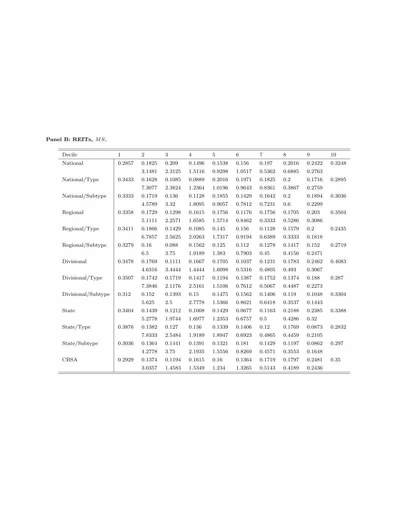
Panel B: REITs, MS.

Decile 1 2 3 4 5 6 7 8 9 10

National 0.2857 0.1825 0.209 0.1496 0.1538 0.156 0.197 0.2016 0.2422 0.3248

3.1481 2.3125 1.5116 0.9298 1.0517 0.5362 0.6885 0.2763

National/Type 0.3433 0.1628 0.1085 0.0889 0.2016 0.1971 0.1825 0.2 0.1716 0.2895

7.3077 2.3824 1.2364 1.0196 0.9643 0.8361 0.3867 0.2759

National/Subtype 0.3333 0.1719 0.136 0.1128 0.1855 0.1429 0.1642 0.2 0.1894 0.3036

4.5789 3.32 1.8095 0.9057 0.7812 0.7231 0.6 0.2299

Regional 0.3358 0.1729 0.1298 0.1615 0.1756 0.1176 0.1756 0.1705 0.203 0.3504

5.1111 2.2571 1.6585 1.5714 0.8462 0.3333 0.5286 0.3086

Regional/Type 0.3411 0.1866 0.1429 0.1085 0.145 0.156 0.1128 0.1579 0.2 0.2435

6.7857 2.5625 2.0263 1.7317 0.9194 0.6389 0.3333 0.1818

Regional/Subtype 0.3279 0.16 0.088 0.1562 0.125 0.112 0.1278 0.1417 0.152 0.2719

6.5 3.75 1.9189 1.383 0.7903 0.45 0.4156 0.2471

Divisional 0.3478 0.1769 0.1111 0.1667 0.1705 0.1037 0.1231 0.1783 0.2462 0.4083

4.6316 3.4444 1.4444 1.6098 0.5316 0.4805 0.493 0.3067

Divisional/Type 0.3507 0.1742 0.1719 0.1417 0.1194 0.1387 0.1752 0.1374 0.188 0.287

7.3846 2.1176 2.5161 1.5106 0.7612 0.5067 0.4487 0.2273

Divisional/Subtype 0.312 0.152 0.1393 0.15 0.1475 0.1562 0.1406 0.119 0.1048 0.3304

5.625 2.5 2.7778 1.5366 0.8621 0.6418 0.3537 0.1443

State 0.3404 0.1439 0.1212 0.1008 0.1429 0.0677 0.1163 0.2188 0.2385 0.3388

5.2778 1.9744 1.6977 1.2353 0.6757 0.5 0.4286 0.32

State/Type 0.3876 0.1382 0.127 0.136 0.1339 0.1406 0.12 0.1769 0.0873 0.2832

7.8333 2.5484 1.9189 1.8947 0.6923 0.4865 0.4459 0.2105

State/Subtype 0.3036 0.1364 0.1441 0.1391 0.1321 0.181 0.1429 0.1197 0.0862 0.297

4.2778 3.75 2.1935 1.5556 0.8269 0.4571 0.3553 0.1648

CBSA 0.2929 0.1374 0.1194 0.1615 0.16 0.1364 0.1719 0.1797 0.2481 0.35

3.0357 1.4583 1.5349 1.234 1.3265 0.5143 0.4189 0.2436

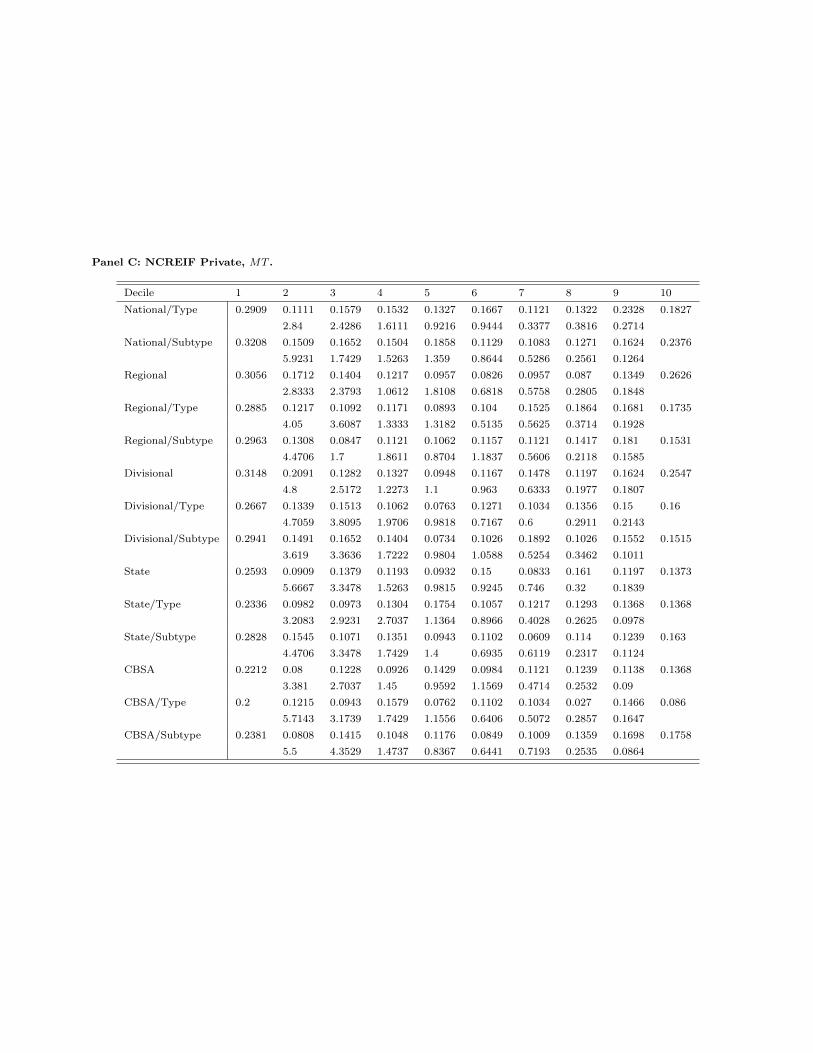
Panel C: NCREIF Private, MT .

Decile 1 2 3 4 5 6 7 8 9 10

National/Type 0.2909 0.1111 0.1579 0.1532 0.1327 0.1667 0.1121 0.1322 0.2328 0.1827

2.84 2.4286 1.6111 0.9216 0.9444 0.3377 0.3816 0.2714

National/Subtype 0.3208 0.1509 0.1652 0.1504 0.1858 0.1129 0.1083 0.1271 0.1624 0.2376

5.9231 1.7429 1.5263 1.359 0.8644 0.5286 0.2561 0.1264

Regional 0.3056 0.1712 0.1404 0.1217 0.0957 0.0826 0.0957 0.087 0.1349 0.2626

2.8333 2.3793 1.0612 1.8108 0.6818 0.5758 0.2805 0.1848

Regional/Type 0.2885 0.1217 0.1092 0.1171 0.0893 0.104 0.1525 0.1864 0.1681 0.1735

4.05 3.6087 1.3333 1.3182 0.5135 0.5625 0.3714 0.1928

Regional/Subtype 0.2963 0.1308 0.0847 0.1121 0.1062 0.1157 0.1121 0.1417 0.181 0.1531

4.4706 1.7 1.8611 0.8704 1.1837 0.5606 0.2118 0.1585

Divisional 0.3148 0.2091 0.1282 0.1327 0.0948 0.1167 0.1478 0.1197 0.1624 0.2547

4.8 2.5172 1.2273 1.1 0.963 0.6333 0.1977 0.1807

Divisional/Type 0.2667 0.1339 0.1513 0.1062 0.0763 0.1271 0.1034 0.1356 0.15 0.16

4.7059 3.8095 1.9706 0.9818 0.7167 0.6 0.2911 0.2143

Divisional/Subtype 0.2941 0.1491 0.1652 0.1404 0.0734 0.1026 0.1892 0.1026 0.1552 0.1515

3.619 3.3636 1.7222 0.9804 1.0588 0.5254 0.3462 0.1011

State 0.2593 0.0909 0.1379 0.1193 0.0932 0.15 0.0833 0.161 0.1197 0.1373

5.6667 3.3478 1.5263 0.9815 0.9245 0.746 0.32 0.1839

State/Type 0.2336 0.0982 0.0973 0.1304 0.1754 0.1057 0.1217 0.1293 0.1368 0.1368

3.2083 2.9231 2.7037 1.1364 0.8966 0.4028 0.2625 0.0978

State/Subtype 0.2828 0.1545 0.1071 0.1351 0.0943 0.1102 0.0609 0.114 0.1239 0.163

4.4706 3.3478 1.7429 1.4 0.6935 0.6119 0.2317 0.1124

CBSA 0.2212 0.08 0.1228 0.0926 0.1429 0.0984 0.1121 0.1239 0.1138 0.1368

3.381 2.7037 1.45 0.9592 1.1569 0.4714 0.2532 0.09

CBSA/Type 0.2 0.1215 0.0943 0.1579 0.0762 0.1102 0.1034 0.027 0.1466 0.086

5.7143 3.1739 1.7429 1.1556 0.6406 0.5072 0.2857 0.1647

CBSA/Subtype 0.2381 0.0808 0.1415 0.1048 0.1176 0.0849 0.1009 0.1359 0.1698 0.1758

5.5 4.3529 1.4737 0.8367 0.6441 0.7193 0.2535 0.0864

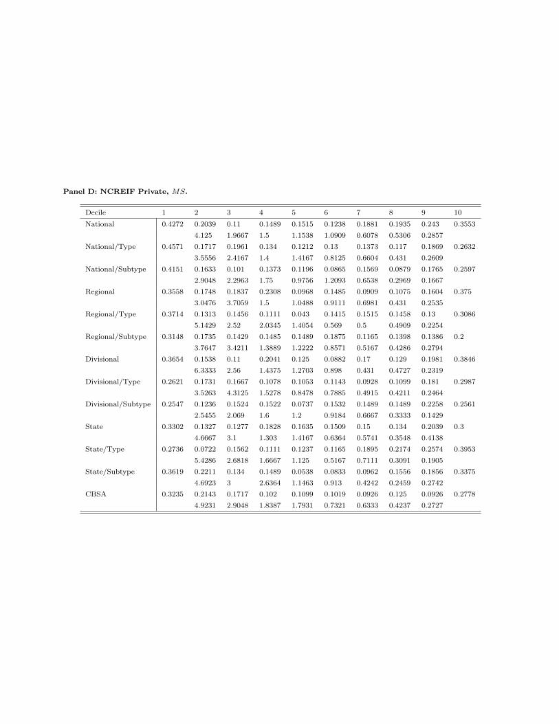
Panel D: NCREIF Private, MS.

Decile 1 2 3 4 5 6 7 8 9 10

National 0.4272 0.2039 0.11 0.1489 0.1515 0.1238 0.1881 0.1935 0.243 0.3553

4.125 1.9667 1.5 1.1538 1.0909 0.6078 0.5306 0.2857

National/Type 0.4571 0.1717 0.1961 0.134 0.1212 0.13 0.1373 0.117 0.1869 0.2632

3.5556 2.4167 1.4 1.4167 0.8125 0.6604 0.431 0.2609

National/Subtype 0.4151 0.1633 0.101 0.1373 0.1196 0.0865 0.1569 0.0879 0.1765 0.2597

2.9048 2.2963 1.75 0.9756 1.2093 0.6538 0.2969 0.1667

Regional 0.3558 0.1748 0.1837 0.2308 0.0968 0.1485 0.0909 0.1075 0.1604 0.375

3.0476 3.7059 1.5 1.0488 0.9111 0.6981 0.431 0.2535

Regional/Type 0.3714 0.1313 0.1456 0.1111 0.043 0.1415 0.1515 0.1458 0.13 0.3086

5.1429 2.52 2.0345 1.4054 0.569 0.5 0.4909 0.2254

Regional/Subtype 0.3148 0.1735 0.1429 0.1485 0.1489 0.1875 0.1165 0.1398 0.1386 0.2

3.7647 3.4211 1.3889 1.2222 0.8571 0.5167 0.4286 0.2794

Divisional 0.3654 0.1538 0.11 0.2041 0.125 0.0882 0.17 0.129 0.1981 0.3846

6.3333 2.56 1.4375 1.2703 0.898 0.431 0.4727 0.2319

Divisional/Type 0.2621 0.1731 0.1667 0.1078 0.1053 0.1143 0.0928 0.1099 0.181 0.2987

3.5263 4.3125 1.5278 0.8478 0.7885 0.4915 0.4211 0.2464

Divisional/Subtype 0.2547 0.1236 0.1524 0.1522 0.0737 0.1532 0.1489 0.1489 0.2258 0.2561

2.5455 2.069 1.6 1.2 0.9184 0.6667 0.3333 0.1429

State 0.3302 0.1327 0.1277 0.1828 0.1635 0.1509 0.15 0.134 0.2039 0.3

4.6667 3.1 1.303 1.4167 0.6364 0.5741 0.3548 0.4138

State/Type 0.2736 0.0722 0.1562 0.1111 0.1237 0.1165 0.1895 0.2174 0.2574 0.3953

5.4286 2.6818 1.6667 1.125 0.5167 0.7111 0.3091 0.1905

State/Subtype 0.3619 0.2211 0.134 0.1489 0.0538 0.0833 0.0962 0.1556 0.1856 0.3375

4.6923 3 2.6364 1.1463 0.913 0.4242 0.2459 0.2742

CBSA 0.3235 0.2143 0.1717 0.102 0.1099 0.1019 0.0926 0.125 0.0926 0.2778

4.9231 2.9048 1.8387 1.7931 0.7321 0.6333 0.4237 0.2727

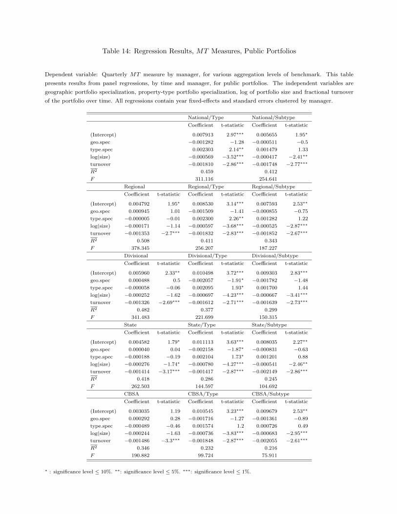
Table 14: Regression Results, MT Measures, Public Portfolios

Dependent variable: Quarterly MT measure by manager, for various aggregation levels of benchmark. This table

presents results from panel regressions, by time and manager, for public portfolios. The independent variables are

geographic portfolio specialization, property-type portfolio specialization, log of portfolio size and fractional turnover

of the portfolio over time. All regressions contain year fixed-effects and standard errors clustered by manager.

National/Type National/Subtype

Coefficient t-statistic Coefficient t-statistic

(Intercept) 0.007913 2.97∗∗∗ 0.005655 1.95∗

geo.spec −0.001282 −1.28 −0.000511 −0.5

type.spec 0.002303 2.14∗∗ 0.001479 1.33

log(size) −0.000569 −3.52∗∗∗ −0.000417 −2.41∗∗

turnover −0.001810 −2.86∗∗∗ −0.001748 −2.77∗∗∗

R2 0.459 0.412

F 311.116 254.641

Regional Regional/Type Regional/Subtype

Coefficient t-statistic Coefficient t-statistic Coefficient t-statistic

(Intercept) 0.004792 1.95∗ 0.008530 3.14∗∗∗ 0.007593 2.53∗∗

geo.spec 0.000945 1.01 −0.001509 −1.41 −0.000855 −0.75

type.spec −0.000005 −0.01 0.002300 2.26∗∗ 0.001282 1.22

log(size) −0.000171 −1.14 −0.000597 −3.68∗∗∗ −0.000525 −2.87∗∗∗

turnover −0.001353 −2.7∗∗∗ −0.001832 −2.83∗∗∗ −0.001852 −2.67∗∗∗

R2 0.508 0.411 0.343

F 378.345 256.207 187.227

Divisional Divisional/Type Divisional/Subtype

Coefficient t-statistic Coefficient t-statistic Coefficient t-statistic

(Intercept) 0.005960 2.33∗∗ 0.010498 3.72∗∗∗ 0.009303 2.83∗∗∗

geo.spec 0.000488 0.5 −0.002057 −1.91∗ −0.001782 −1.48

type.spec −0.000058 −0.06 0.002095 1.93∗ 0.001700 1.44

log(size) −0.000252 −1.62 −0.000697 −4.23∗∗∗ −0.000667 −3.41∗∗∗

turnover −0.001326 −2.69∗∗∗ −0.001612 −2.71∗∗∗ −0.001639 −2.73∗∗∗

R2 0.482 0.377 0.299

F 341.483 221.699 150.315

State State/Type State/Subtype

Coefficient t-statistic Coefficient t-statistic Coefficient t-statistic

(Intercept) 0.004582 1.79∗ 0.011113 3.63∗∗∗ 0.008035 2.27∗∗

geo.spec 0.000040 0.04 −0.002158 −1.87∗ −0.000831 −0.63

type.spec −0.000188 −0.19 0.002104 1.73∗ 0.001201 0.88

log(size) −0.000276 −1.74∗ −0.000780 −4.27∗∗∗ −0.000541 −2.46∗∗

turnover −0.001414 −3.17∗∗∗ −0.001417 −2.87∗∗∗ −0.002149 −2.86∗∗∗

R2 0.418 0.286 0.245

F 262.503 144.597 104.692

CBSA CBSA/Type CBSA/Subtype

Coefficient t-statistic Coefficient t-statistic Coefficient t-statistic

(Intercept) 0.003035 1.19 0.010545 3.23∗∗∗ 0.009679 2.53∗∗

geo.spec 0.000292 0.28 −0.001716 −1.27 −0.001361 −0.89

type.spec −0.000489 −0.46 0.001574 1.2 0.000726 0.49

log(size) −0.000244 −1.63 −0.000736 −3.83∗∗∗ −0.000683 −2.95∗∗∗

turnover −0.001486 −3.3∗∗∗ −0.001848 −2.87∗∗∗ −0.002055 −2.61∗∗∗

R2 0.346 0.232 0.216

F 190.882 99.724 75.911

∗ : significance level ≤ 10%. ∗∗: significance level ≤ 5%. ∗∗∗: significance level ≤ 1%.

Table 15: Regression Results, MT Measures, Private Portfolios

Dependent variable: Quarterly MT measure by manager, for various aggregation levels of benchmark. This table

presents results from panel regressions, by time and manager, for private portfolios. The independent variables are

geographic portfolio specialization, property-type portfolio specialization, log of portfolio size and fractional turnover

of the portfolio over time. All regressions contain year fixed-effects and standard errors clustered by manager.

National/Type National/Subtype

Coefficient t-statistic Coefficient t-statistic

(Intercept) −0.007710 −2.01∗∗ −0.006309 −1.48

geo.spec 0.002269 1.9∗ 0.002644 2.03∗∗

type.spec −0.001367 −1.34 −0.001646 −1.52

log(size) 0.000390 2.11∗∗ 0.000315 1.53

turnover −0.000921 −2.96∗∗∗ −0.000795 −2.49∗∗

R2 0.56 0.548

F 195.593 185.88

Regional Regional/Type Regional/Subtype

Coefficient t-statistic Coefficient t-statistic Coefficient t-statistic

(Intercept) −0.010816 −2.59∗∗∗ −0.008428 −2.13∗∗ −0.006272 −1.34

geo.spec 0.002895 2.44∗∗ 0.001947 1.43 0.002827 1.76∗

type.spec −0.000769 −0.77 −0.001821 −1.64 −0.002160 −1.81∗

log(size) 0.000497 2.61∗∗∗ 0.000377 1.92∗ 0.000276 1.29

turnover −0.000774 −2.81∗∗∗ −0.000820 −2.74∗∗∗ −0.000743 −2.25∗∗

R2 0.557 0.536 0.503

F 193.063 177.683 155.196

Divisional Divisional/Type Divisional/Subtype

Coefficient t-statistic Coefficient t-statistic Coefficient t-statistic

(Intercept) −0.007972 −1.47 −0.009355 −2.14∗∗ −0.004774 −0.95

geo.spec 0.002994 1.98∗∗ 0.001773 1.05 0.003646 1.76∗

type.spec −0.000964 −0.93 −0.001432 −1.22 −0.002421 −1.89∗

log(size) 0.000504 2.42∗∗ 0.000432 2∗∗ 0.000342 1.43

turnover −0.000648 −2.32∗∗ −0.000694 −2.21∗∗ −0.000639 −1.89∗

R2 0.547 0.518 0.494

F 185.742 165.44 147.501

State State/Type State/Subtype

Coefficient t-statistic Coefficient t-statistic Coefficient t-statistic

(Intercept) −0.006485 −1.24 −0.009941 −1.94∗ −0.001818 −0.31

geo.spec 0.002285 1.19 0.003686 2.08∗∗ 0.004750 1.78∗

type.spec −0.001567 −1.47 −0.001717 −1.42 −0.001448 −1.03

log(size) 0.000362 1.53 0.000512 2.1∗∗ 0.000582 2.16∗∗

turnover −0.000786 −2.7∗∗∗ −0.000819 −2.35∗∗ −0.000796 −2.28∗∗

R2 0.519 0.462 0.442

F 165.778 131.366 117.464

CBSA CBSA/Type CBSA/Subtype

Coefficient t-statistic Coefficient t-statistic Coefficient t-statistic

(Intercept) −0.006814 −1.2 −0.005732 −1.02 −0.000977 −0.14

geo.spec 0.002767 1.38 0.001823 0.92 0.002664 0.8

type.spec −0.001659 −1.51 −0.001255 −0.95 −0.001162 −0.74

log(size) 0.000436 1.85∗ 0.000505 1.91∗ 0.000490 1.5

turnover −0.000756 −2.1∗∗ −0.000912 −2.19∗∗ −0.000912 −2.09∗∗

R2 0.494 0.424 0.417

F 147.33 109.84 101.723

∗ : significance level ≤ 10%. ∗∗: significance level ≤ 5%. ∗∗∗: significance level ≤ 1%.

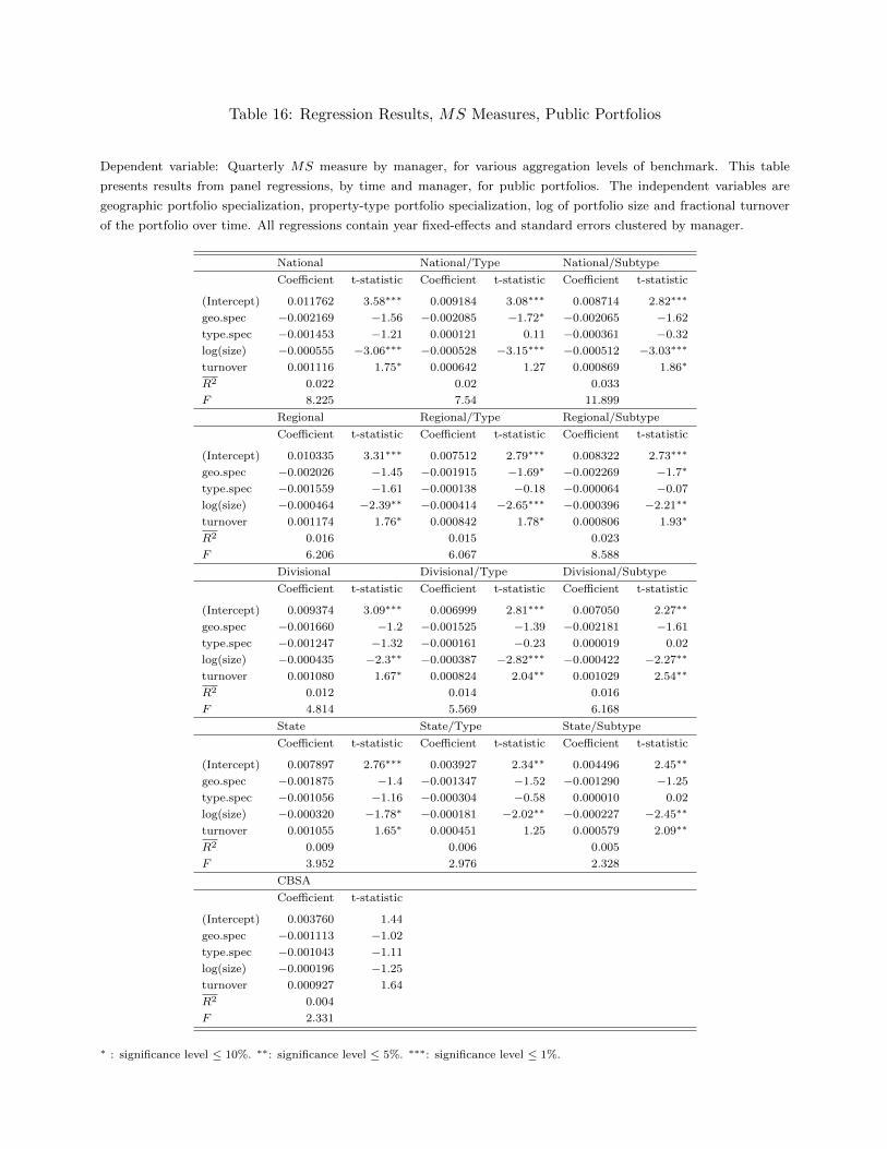
Table 16: Regression Results, MS Measures, Public Portfolios

Dependent variable: Quarterly MS measure by manager, for various aggregation levels of benchmark. This table

presents results from panel regressions, by time and manager, for public portfolios. The independent variables are

geographic portfolio specialization, property-type portfolio specialization, log of portfolio size and fractional turnover

of the portfolio over time. All regressions contain year fixed-effects and standard errors clustered by manager.

National National/Type National/Subtype

Coefficient t-statistic Coefficient t-statistic Coefficient t-statistic

(Intercept) 0.011762 3.58∗∗∗ 0.009184 3.08∗∗∗ 0.008714 2.82∗∗∗

geo.spec −0.002169 −1.56 −0.002085 −1.72∗ −0.002065 −1.62

type.spec −0.001453 −1.21 0.000121 0.11 −0.000361 −0.32

log(size) −0.000555 −3.06∗∗∗ −0.000528 −3.15∗∗∗ −0.000512 −3.03∗∗∗

turnover 0.001116 1.75∗ 0.000642 1.27 0.000869 1.86∗

R2 0.022 0.02 0.033

F 8.225 7.54 11.899

Regional Regional/Type Regional/Subtype

Coefficient t-statistic Coefficient t-statistic Coefficient t-statistic

(Intercept) 0.010335 3.31∗∗∗ 0.007512 2.79∗∗∗ 0.008322 2.73∗∗∗

geo.spec −0.002026 −1.45 −0.001915 −1.69∗ −0.002269 −1.7∗

type.spec −0.001559 −1.61 −0.000138 −0.18 −0.000064 −0.07

log(size) −0.000464 −2.39∗∗ −0.000414 −2.65∗∗∗ −0.000396 −2.21∗∗

turnover 0.001174 1.76∗ 0.000842 1.78∗ 0.000806 1.93∗

R2 0.016 0.015 0.023

F 6.206 6.067 8.588

Divisional Divisional/Type Divisional/Subtype

Coefficient t-statistic Coefficient t-statistic Coefficient t-statistic

(Intercept) 0.009374 3.09∗∗∗ 0.006999 2.81∗∗∗ 0.007050 2.27∗∗

geo.spec −0.001660 −1.2 −0.001525 −1.39 −0.002181 −1.61

type.spec −0.001247 −1.32 −0.000161 −0.23 0.000019 0.02

log(size) −0.000435 −2.3∗∗ −0.000387 −2.82∗∗∗ −0.000422 −2.27∗∗

turnover 0.001080 1.67∗ 0.000824 2.04∗∗ 0.001029 2.54∗∗

R2 0.012 0.014 0.016

F 4.814 5.569 6.168

State State/Type State/Subtype

Coefficient t-statistic Coefficient t-statistic Coefficient t-statistic

(Intercept) 0.007897 2.76∗∗∗ 0.003927 2.34∗∗ 0.004496 2.45∗∗

geo.spec −0.001875 −1.4 −0.001347 −1.52 −0.001290 −1.25

type.spec −0.001056 −1.16 −0.000304 −0.58 0.000010 0.02

log(size) −0.000320 −1.78∗ −0.000181 −2.02∗∗ −0.000227 −2.45∗∗

turnover 0.001055 1.65∗ 0.000451 1.25 0.000579 2.09∗∗

R2 0.009 0.006 0.005

F 3.952 2.976 2.328

CBSA

Coefficient t-statistic

(Intercept) 0.003760 1.44

geo.spec −0.001113 −1.02

type.spec −0.001043 −1.11

log(size) −0.000196 −1.25

turnover 0.000927 1.64

R2 0.004

F 2.331

∗ : significance level ≤ 10%. ∗∗: significance level ≤ 5%. ∗∗∗: significance level ≤ 1%.

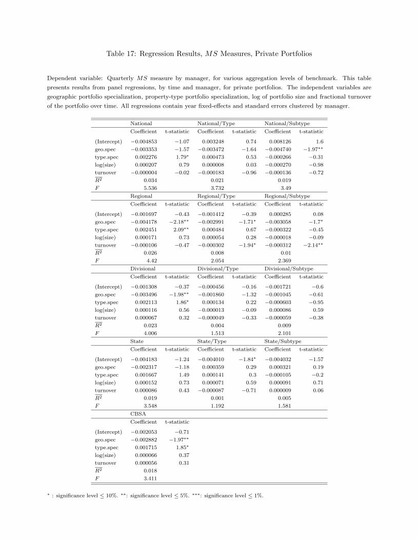
Table 17: Regression Results, MS Measures, Private Portfolios

Dependent variable: Quarterly MS measure by manager, for various aggregation levels of benchmark. This table

presents results from panel regressions, by time and manager, for private portfolios. The independent variables are

geographic portfolio specialization, property-type portfolio specialization, log of portfolio size and fractional turnover

of the portfolio over time. All regressions contain year fixed-effects and standard errors clustered by manager.

National National/Type National/Subtype

Coefficient t-statistic Coefficient t-statistic Coefficient t-statistic

(Intercept) −0.004853 −1.07 0.003248 0.74 0.008126 1.6

geo.spec −0.003353 −1.57 −0.003472 −1.64 −0.004740 −1.97∗∗

type.spec 0.002276 1.79∗ 0.000473 0.53 −0.000266 −0.31

log(size) 0.000207 0.79 0.000008 0.03 −0.000270 −0.98

turnover −0.000004 −0.02 −0.000183 −0.96 −0.000136 −0.72

R2 0.034 0.021 0.019

F 5.536 3.732 3.49

Regional Regional/Type Regional/Subtype

Coefficient t-statistic Coefficient t-statistic Coefficient t-statistic

(Intercept) −0.001697 −0.43 −0.001412 −0.39 0.000285 0.08

geo.spec −0.004178 −2.18∗∗ −0.002991 −1.71∗ −0.003058 −1.7∗

type.spec 0.002451 2.09∗∗ 0.000484 0.67 −0.000322 −0.45

log(size) 0.000171 0.73 0.000054 0.28 −0.000018 −0.09

turnover −0.000106 −0.47 −0.000302 −1.94∗ −0.000312 −2.14∗∗

R2 0.026 0.008 0.01

F 4.42 2.054 2.369

Divisional Divisional/Type Divisional/Subtype

Coefficient t-statistic Coefficient t-statistic Coefficient t-statistic

(Intercept) −0.001308 −0.37 −0.000456 −0.16 −0.001721 −0.6

geo.spec −0.003496 −1.98∗∗ −0.001860 −1.32 −0.001045 −0.61

type.spec 0.002113 1.86∗ 0.000134 0.22 −0.000603 −0.95

log(size) 0.000116 0.56 −0.000013 −0.09 0.000086 0.59

turnover 0.000067 0.32 −0.000049 −0.33 −0.000059 −0.38

R2 0.023 0.004 0.009

F 4.006 1.513 2.101

State State/Type State/Subtype

Coefficient t-statistic Coefficient t-statistic Coefficient t-statistic

(Intercept) −0.004183 −1.24 −0.004010 −1.84∗ −0.004032 −1.57

geo.spec −0.002317 −1.18 0.000359 0.29 0.000321 0.19

type.spec 0.001667 1.49 0.000141 0.3 −0.000105 −0.2

log(size) 0.000152 0.73 0.000071 0.59 0.000091 0.71

turnover 0.000086 0.43 −0.000087 −0.71 0.000009 0.06

R2 0.019 0.001 0.005

F 3.548 1.192 1.581

CBSA

Coefficient t-statistic

(Intercept) −0.002053 −0.71

geo.spec −0.002882 −1.97∗∗

type.spec 0.001715 1.85∗

log(size) 0.000066 0.37

turnover 0.000056 0.31

R2 0.018

F 3.411

∗ : significance level ≤ 10%. ∗∗: significance level ≤ 5%. ∗∗∗: significance level ≤ 1%.