markov switching garch models of currency … switching garch models of currency turmoil in...

Board of Governors of the Federal Reserve System

International Finance Discussion Papers

Number 889

January 2007

Markov Switching GARCH Models of Currency Turmoil in Southeast Asia

Celso Brunetti Roberto S. Mariano

Chiara Scotti Augustine H.H. Tan

NOTE: International Finance Discussion Papers are preliminary materials circulated to stimulate discussion and critical comment. References in publications to International Finance Discussion Papers (other than an acknowledgment that the writer has had access to unpublished material) should be cleared with the author or authors. Recent IFDPs are available on the Web at www.federalreserve.gov/pubs/ifdp/. This paper can be downloaded without charge from Social Science Research Network electronic library at http://www.ssrn.com/.

http://www.federalreserve.gov/pubs/ifdp/

MARKOV SWITCHING GARCH MODELS OF CURRENCY

TURMOIL IN SOUTHEAST ASIA

Celso BrunettiJohns Hopkins University

Roberto S. MarianoSingapore Management University

Chiara ScottiFederal Reserve Board

Augustine H.H. TanSingapore Management University

January 2007 �

Abstract

This paper analyzes exchange rate turmoil with a Markov Switching GARCH model. We

distinguish between two di¤erent regimes in both the conditional mean and the conditional

variance: �ordinary�regime, characterized by low exchange rate changes and low volatility,

and �turbulent�regime, characterized by high exchange rate movements and high volatility.

We also allow the transition probabilities to vary over time as functions of economic and

�nancial indicators. We �nd that real e¤ective exchange rates, money supply relative to

reserves, stock index returns, and bank stock index returns and volatility contain valuable

information for identifying turbulence and ordinary periods.

Keywords: Currency crises; Financial markets; Banking sector; Regime switching; Volatil-

ity.

JEL classi�cation: C13; C22; C52; F31; F34.

�We would like to thank for helpful comments: Mark Carey, Graciela Kaminsky, Adrian Pagan, Jon Wongswan,and participants at the EC2 conference in Bologna 2002 and ASSA meeting in Washington DC 2003. The authorsgratefully acknowledge funding support from the Wharton Singapore Management University Research Center.The views expressed in this paper are solely the responsibility of the authors and should not be interpreted asre�ecting the view of the Board of Governors of the Federal Reserve System or of any other person associatedwith the Federal Reserve System.

1

1 Introduction

The decade of the nineties witnessed several bank and currency crises.1 The severity of the crises

has motivated researchers to develop early warning systems in order to forestall similar crises.

Such early warning systems typically involve some precise de�nition of a crisis and a mechanism

for predicting it. A currency crisis is usually identi�ed as an episode in which there is a sharp

depreciation of the currency, a large decline in foreign reserves, a dramatic increase in domestic

interest rates or a combination of these elements.

This paper studies exchange rate turmoil, that is, we focus on episodes of extensive ex-

change rate changes, and we analyze which variables trigger the move from a tranquil period to

a turbulent time. Since a currency crisis is not necessarily a turbulent period, and vice versa,

our approach identi�es currency crises only when they manifest with large exchange rate de-

valuations. Our modeling strategy relies on the empirical evidence that i) small exchange rate

changes are associated with low volatility (ordinary regime) and large exchange rate movements

go together with high volatility (turbulence), and ii) exchange rate volatility is not constant in

the two regimes. This calls for a GARCH regime switching approach, in which we furthermore

allow the transition probabilities to vary over time as functions of economic and �nancial indi-

cators. Switching volatility models have been used for modeling equity markets (Hamilton and

Susmel, 1994; Dueker, 1997; Susmel, 2000), short-term interest rates (Cai, 1994; Gray, 1996;

Kalimipalli and Susmel, 2006), emerging equity markets (Susmel, 1998), and exchange rates

(Klaassen, 2002; Calvet and Fisher, 2004). However, to the best of our knowledge, this paper is

the �rst application to currency turmoil.

The analysis is applied to four Southeast Asian countries: Thailand, Singapore, the Philip-

pines, and Malaysia. Estimation results support our intuition for modeling exchange rate volatil-

ities. Our results, in fact, show that signals of the July 1997 crisis become apparent in Thailand

as early as January, and the probability of getting into a crisis jumps to as much as 82 percent

in June 1997.

The literature on �nancial/currency crises is vast, and it mainly focuses on trying to predict

crises in developing countries. There are three methods or approaches for predicting currency

crises that have been developed in the literature.

One class of models is the probit regression approach of Frankel and Rose (1996). They

use probit analysis on a panel of annual data for 105 developing countries from 1971-92. The

hypothesis tested is that currency crashes are positively linked to certain characteristics of capital

in�ows, such as low shares of foreign direct investments (FDI); low shares of concessional debt or

debt from multilateral development banks; and high shares of public-sector, variable short-term,

1Europe in 1992-93 (the European Exchange Rate mechanism); Mexico in 1994-95; Turkey in 1994 and 2000-01;East and Southeast Asia in 1997; Russia in 1998; and Argentina, Uruguay and Brazil starting in late 2001.

2

and commercial bank debt. The �nding is that currency crises are more likely when foreign

interest rates are high, domestic credit growth is high, the real exchange rate is overvalued, the

current account de�cit and �scal de�cit are large (as a share of GDP), external concessional debt

is small, and FDI is small in relation to the total volume of external debt. However, when the

model is used to generate out-of-sample predictions for the 1997 Asian Crisis, the forecasts are

not successful (Berg and Patillo, 1999a).2 More recently Bussiere and Fratzcher (2006) develop a

new early warning system model based on a multinomial logit with three outcomes (tranquil, pre-

crisis and post-crisis) showing that such a speci�cation leads to a better out-of-sample forecast

and solves what they call the �post-crisis bias.�

A second class of models (Tornell, 1999; IMF, World Economic Outlook, 1998; Radelet and

Sachs, 1998; Corsetti Pesenti and Roubini,1999) follows Sachs, Tornell and Velasco (1996) who

use cross-country regressions to explain the Tequila (Mexican) crisis of 1995. Using a crisis index

de�ned as the weighted sum of the percentage decrease in foreign reserves and the percentage

depreciation of the peso, they conclude that countries have more severe attacks when they have

low foreign reserves, their banking systems are weak and their currencies overvalued. Berg and

Patillo (1999a) extend the data to 23 other countries and conclude that the Sachs, Tornell and

Velasco (1996) model proved to be largely unstable. Speci�cation uncertainty appeared to be

as important as parameter uncertainty.

The third class of models, attributed to Kaminsky, Lizondo and Reinhart (1998), is the

�signals approach.�A crisis is de�ned as a situation in which a weighted average of monthly

percentage depreciations in the currency and monthly percentage declines in reserves exceeds

its mean by more than three standard deviations. They use 15 monthly variables to monitor for

unusual behavior during a 24-month window prior to a crisis. Threshold levels, beyond which

signals would be generated, are speci�ed. Using variants of the signals approach, Kaminsky

(1998a and 1998b), Kaminsky and Reinhart (1999), and Goldstein, Kaminsky and Reinhart

(2000) claim some success in predicting the Asian crisis.

These approaches have some limitations. For example, the signal approach requires the

ex-ante de�nition of a threshold and the transformation of the variables into binary variables,

with a signi�cant loss of information; the logit/probit approach requires the de�nition of a crisis

dummy, with potential misclassi�cations.

We use a Markov switching approach in which we account for the presence of two potential

regimes: ordinary and turbulent. We also recognize the fact that, even within each regime,

the volatility of exchange rate returns is not constant, and we therefore include a GARCH

2See also Berg and Patillo (1999b). A more recent paper by Kumar, Moorthy and Perraudin, 2003, appliedlogit models to pooled data on 32 developing countries for the period January 1985 to October 1999. The resultscon�rm those of earlier studies that factors such as declining reserves, exports and declining real activity are themost important explanatory variables for currency crashes.

3

speci�cation. The probabilities of switching between the two regimes are time-varying. The

attractiveness of this approach is that we do not need to distinguish ex-ante between ordinary

and turbulent times, but we let the estimation results supply us with this information. We

di¤er from Mariano et al. (2002) in that we recognize the importance of volatility dynamics,

and we enlarge the set of potential explanatory variables to include the M2-reserve ratio, real

domestic credit, real e¤ective exchange rate, stock market returns and volatility, and banking

sector returns and volatility.

The model can be used for out-of-sample forecasting. Unfortunately, the short sample does

not allow us to do so in the current paper (GARCH models require long datasets). Therefore,

we only limit our study to understanding the variables and modeling speci�cations which play

a role in comprehending currency turmoil, leaving the out-of-sample forecast exercise to future

assessment.

This paper proceeds in Section 2 by motivating the use of a Markov switching GARCH

model. Section 3 presents the model. Section 4 illustrates the data used in the estimation.

Section 5 presents the estimation results toghether with an analysis of the estimated time-

varying transition probabilities. Section 6 concludes the paper.

2 Motivating our Approach

The goal of the paper is to study episodes of high (low) risk and high (low) exchange rate

movements.

Our approach consists in modeling the conditional mean and the conditional variance of the

exchange rate devaluation. The �rst and the second order moments of exchange rate devaluation

are driven by the same Markov process governed by an unobservable state variable. The under-

lying assumption is quite simple: low mean values of exchange rate devaluation are associated

with low volatility of the exchange rate devaluation, and high devaluation is associated with high

volatility. We refer to the latter regime as �turbulence�and the former as describing �ordinary�

market conditions. In addition, the transition probabilities in the Markov process are functions

of macroeconomic and/or �nancial variables. This captures the idea that large exchange rate

devaluations and high risk might be driven by exogenous variables.

This approach might lead to identify currency crises. In fact, there is empirical evidence (see

below) showing that, at least for the four Southeast Asian countries analyzed in this paper, high

risk and high exchange rate devaluation correspond indeed to the 1997 currency crises.

The countries considered are Thailand, Singapore, Malaysia and Philippines. The sample

period runs from November 1984 to December 2001.

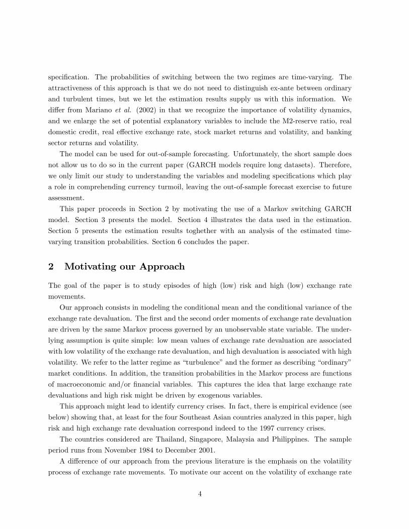
A di¤erence of our approach from the previous literature is the emphasis on the volatility

process of exchange rate movements. To motivate our accent on the volatility of exchange rate

4

returns, we compute a volatility proxy: the range,3 which is de�ned as the di¤erence between the

maximum value of the (log of the) price process over a given interval of time and the minimum

value of the (log of the) price process over the same interval

l = max0�n�N

[ln(Pn)]� min0�n�N

[ln(Pn)] (1)

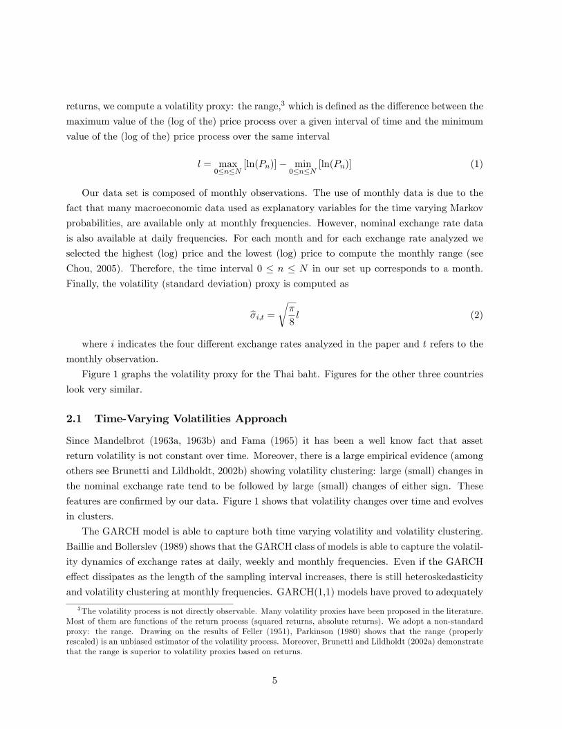
Our data set is composed of monthly observations. The use of monthly data is due to the

fact that many macroeconomic data used as explanatory variables for the time varying Markov

probabilities, are available only at monthly frequencies. However, nominal exchange rate data

is also available at daily frequencies. For each month and for each exchange rate analyzed we

selected the highest (log) price and the lowest (log) price to compute the monthly range (see

Chou, 2005). Therefore, the time interval 0 � n � N in our set up corresponds to a month.

Finally, the volatility (standard deviation) proxy is computed as

b�i;t =r�8l (2)

where i indicates the four di¤erent exchange rates analyzed in the paper and t refers to the

monthly observation.

Figure 1 graphs the volatility proxy for the Thai baht. Figures for the other three countries

look very similar.

2.1 Time-Varying Volatilities Approach

Since Mandelbrot (1963a, 1963b) and Fama (1965) it has been a well know fact that asset

return volatility is not constant over time. Moreover, there is a large empirical evidence (among

others see Brunetti and Lildholdt, 2002b) showing volatility clustering: large (small) changes in

the nominal exchange rate tend to be followed by large (small) changes of either sign. These

features are con�rmed by our data. Figure 1 shows that volatility changes over time and evolves

in clusters.

The GARCH model is able to capture both time varying volatility and volatility clustering.

Baillie and Bollerslev (1989) shows that the GARCH class of models is able to capture the volatil-

ity dynamics of exchange rates at daily, weekly and monthly frequencies. Even if the GARCH

e¤ect dissipates as the length of the sampling interval increases, there is still heteroskedasticity

and volatility clustering at monthly frequencies. GARCH(1,1) models have proved to adequately

3The volatility process is not directly observable. Many volatility proxies have been proposed in the literature.Most of them are functions of the return process (squared returns, absolute returns). We adopt a non-standardproxy: the range. Drawing on the results of Feller (1951), Parkinson (1980) shows that the range (properlyrescaled) is an unbiased estimator of the volatility process. Moreover, Brunetti and Lildholdt (2002a) demonstratethat the range is superior to volatility proxies based on returns.

5

describe exchange rate volatility dynamics.4 This is the approach we follow in this paper.

2.2 Markov Regime Switching Approach

As already stated, we model jointly the conditional mean and the conditional variance (volatility)

of exchange rate devaluations. The Markov switching regime model adopted relies on two

assumptions: i) the volatility process is characterized by two regimes, high volatility and low

volatility; ii) the high volatility regime is associated with large exchange rate deviations (high

values of the mean process) and the low volatility regime is associated with small exchange rate

movements (low values of the mean process). The �rst assumption is con�rmed by Figure 1. For

all of the four countries analyzed, the volatility process exhibits periods of very low volatility

and periods of very high volatility. Interestingly, the highest volatilities coincide with the 1997

crisis which is the major currency crisis that took place during our sample. Therefore this crisis

represents our benchmark.

The onset of the crisis in Thailand, the �rst country to be hit by the crisis, was on July 1997.

The average monthly volatility (standard deviation) in the 12 months after the crisis (July 1997

- June 1998) was more than seven times bigger than in the previous 12 months (July 1996 - June

1997). Similar results also apply to Singapore and Malaysia. For the Philippines the volatility

in the twelve months subsequent the beginning of the crisis increased by a factor of 55.

The second assumption simply implies that the same Markov process drives both the mean

and the variance of exchange rate returns. Figure 2 displays the scatter plot of exchange rate

devaluation and the volatility proxy for Thailand. It is evident that periods of zero or low

exchange rate devaluation/appreciation are associated with low risk and periods of severe deval-

uations are associated with very high exchange rate risk. In the twelve months after the onset

of the 1997 crisis the level of the exchange rate devaluation increased by a factor of 8 compared

to the 12 months before. Similar results apply to the other three countries. The exchange rate

devaluation increased by a factor of 12, 59 and 54 in Singapore, the Philippines and Malaysia

respectively, when comparing the twelve months before and after the crisis.

It is interesting to note the asymmetry of exchange rate devaluation and volatility: in periods

of high risk the currency devaluates. The largest outliers in Figure 2 refer to the 1997 crisis.

The presence of two regimes - low devaluation and low volatility versus high devaluation

and high volatility - motivates the Markov switching approach adopted. It is also evident that

within the two regimes volatility is not constant. Hence the need for a GARCH approach.

4For a review of the literature on GARCH models see Bera and Higgins (1993) and Bollerslev, Engle and Nelson(1994). More recently, see Hansen and Lunde (2005), who show that a GARCH(1,1) cannot be outperformed bymore sophisticated models in the analysis of exchange rates.

6

2.3 Turbulence and Crisis

The modeling strategy adopted is able to identify turbulent periods. Do turbulent periods

correspond to currency crises?

A currency crisis is not necessarily a turbulent period, and vice versa. There can be a crisis

without any exchange rate devaluation (and of course without any volatility of the exchange

rate devaluation). In fact, the government might be able to absorb exchange rate pressures

using foreign reserves, interest rates, etc. On the same base the exchange rate might experience

turbulence without being in a crisis.

Citing Kaminsky and Reinhart (1999): �Most often, balance-of-payments crises are resolved

through a devaluation of the domestic currency or the �otation of the exchange rate. But central

banks can and, on occasion, do resort to contractionary monetary policy and foreign-exchange

market intervention to �ght speculative attack�(p.475-6).

Figures 1 and 2 provide overwhelming evidence that the 1997 crisis resolved in a large

exchange rate devaluation and high volatility. Our modeling approach distinguishes between

turbulent and ordinary periods and identi�es currency crises only to the extent that they manifest

with large exchange rate devaluations.

3 Time varying probabilities Markov switching GARCHmodels

Let yt be the �rst di¤erence of the log nominal exchange rate. The simple GARCH(1,1) model

may be written as follows:

yt = �+

kXi=1

�iXi;t + ut (3)

ut = �t"t; "t � nid(0; 1) (4)

�2t jt�1 = ! + �u2t�1 + ��2t�1 (5)

where Xi are the exogenous and/or lagged variables for the mean of the returns, � is the

corresponding parameter vector and t�1 is the information set available at time t � 1. Forsimplicity we are assuming that the innovation term follows a normal distribution. The model

is very �exible, and many extensions have been proposed in the literature.

As shown in the previous section, in periods of currency turbulence, exchange rate volatility

is often very high ,and we may distinguish between two regimes: a �ordinary� regime and a

�turbulence�regime. The approach we adopt here is similar to Gray (1996) and Dueker (1997).

Equations 3-5 can be written as

7

yt = �t +kXi=1

�iXit + ut (6)

ut = �t"t; "t � nid(0; 1) (7)

�2t (St; St�1:::S0) = ! (St) + � (St�1)u2t�1 + � (St�1)�

2t�1 (St�1:::S0) (8)

The constant, �t, in the conditional mean equation is allowed to switch between two regimes

- high mean (�1) and low mean (�0),

�t = �1St + �0 (1� St) (9)

St 2 f0; 1g ; 8t (10)

Pr (St = 0jSt�1 = 0) = p (11)

Pr (St = 1jSt�1 = 1) = q (12)

where St is the latent Markov chain of order one. We are assuming that the parameter vector

� in the conditional mean equation is constant (i.e. it does not switch according to the Markov

process), but this assumption can be easily relaxed. The innovation term, ut, follows a normal

distribution.

The conditional variance, �2t , is a function of the entire history of the state variable. This is

due to the autoregressive term, �2t�1, in the conditional variance equation - see Dueker (1997),

Cai (1994) and Hamilton and Susmel (1994). Obviously, it is very demanding to account for

all the past history of the state variable. Following Dueker (1997), we adopt an approxima-

tion procedure that seems not to cause any problems in the evaluation of the likelihood func-

tion. This procedure implies that the conditional variance is a function of only the most recent

values of the state variable. Dueker (1997) shows that in a GARCH(1,1) model we need to

consider only the most recent four values of the state variable. This means that the condi-

tional variance, �2t , is function only of the current state (St) and the previous state (St�1):

�2t (i; j) = �2t (St = i; St�1 = j). By integrating out St�1, the conditional variance can be writ-

ten as

�2t (i; j) = ! (St = i) + ��u2t�1 (j)

�+ �

��2t�1 (j)

�(13)

Equation (13) implies that the constant in the conditional variance equation is allowed

to switch. In the GARCH(1,1) speci�cation, the unconditional variance is given by !1�� .

Therefore, equation (13) allows two unconditional variances: high unconditional variance in

�turbulence�regimes and low unconditional variance in �ordinary�regimes. Following Dueker

(1997), ! (St) is parameterized as g (St)! such that g (S = 0) is normalized to unity.

8

In this setup the transition probabilities are constant. This seems over-restrictive. Transition

probabilities may depend on economic variables. For this reason we introduce time varying

probabilities. In our setup transition probabilities are probit functions of economic variables

denoted by Zt

Pr (St = 0jSt�1 = 0) = p = ��Z0t�1�

�(14)

Pr (St = 1jSt�1 = 1) = q = ��Z0t�1�

�(15)

where � denotes the cdf of the normal distribution. A Markov switching regime GARCH

model with time varying probabilities is also developed in Gray (1996).

This approach allows forecasting the conditional probability of being in a given regime (i; j)

at time t+ 1 given the information available at time t.

Denote^�tjt the (N � 1) vector of conditional probabilities of being in state (0; 1) conditional

on the data until date t. De�ne �t as the (N � 1) vector of the density of yt conditional on St.Following Hamilton (1994), the optimal forecast for each t is computed by iterating the following

two equations

b�tjt =

�^�tjt�1 � �t

�10�^�tjt�1 � �t

� (16)

b�t+1jt = Pt+1�^�tjt (17)

where 1 is the unit vector, Pt+1 is the (N �N) Markov transition probability matrix and� denotes the element-by-element multiplication.

Recall that Pt is time varying and depends on the previous period values of explanatory

variables. We are mainly interested in the turbulent regime. Our approach allows us to compute

the probability of moving to a turbulence regime in period t+1 given all the available information

at time t.

The log-likelihood function is given by

lnLt (i; j) = �1

2ln��2t (j)

�+ ln

�u2t�1 (i)

�2t (j)

�� ln

hp2�i

(18)

where i 2 f0; 1g relates to St 2 f0; 1g and j 2 f0; 1g relates to St�1 2 f0; 1g. The functionis maximized following Hamilton (1994).

9

4 Data Description

Currency crises/turmoil most often reveal themselves in an actual devaluation of the domestic

currency or the �otation of the exchange rate. Nevertheless, there are occasions in which central

banks wind up adopting contractionary policies. In these cases, crises manifest themselves in

interest rate hikes, depletion of reserves, etc. Also, currency crises are sometimes linked to

banking/�nancial sector distresses.5

To take into account all facets of currency turmoil, we consider a number of macroeconomic

and �nancial variables: M2/reserves, real domestic credit, real e¤ective exchange rate, banking

sector stock index returns and volatility, general stock market index returns and volatility.6 In

order to get a clearer view of the evolution of turbulent periods we use monthly data, from

November 1984 to December 2001.7

Exchange rates devaluation/appreciation is simply computed using end of the month log-�rst

di¤erence.

Real e¤ective exchange rate (REER) and interest rate di¤erentials (IRDIFF) are external

sector indicators. In particular, the percentage deviation of the REER from a trend is a current

account indicator, while the domestic-US real interest rate di¤erential on deposits represents an

indicator associated with the capital account. REER is considered as deviation from a trend

because not all real appreciations/depreciations necessarily re�ect disequilibrium phenomena.

M2/reserves (M2 ratio) together with real domestic credit/GDP (RDC) are �nancial sector

indicators. Both variables are considered in deviation from a trend. In fact, not all the changes

in those indicators are symptomatic of a troublesome situation.8

Stock index returns (GENRET) and volatility (GENVOL) are indicators of the real sector9

linking currency turmoil to economic activity.

In order to stress the link between currency crises and banking problems we introduce returns

and volatility of a stock index based on a portfolio (weighted by the capitalization) of banks listed

on the stock market (BANKRET and BANKVOL, respectively).10 We believe these variables

could be important indicators for the Southeast Asian crisis we study in this paper.

Citing Kaminsky and Reinhart, �Of course, this is not an exhaustive list of potential in-

dicators� (p.481). We have considered only some of the indicators that they suggest and add

5For a literature review on the link between banking and currency crisis see Kaminsky and Reinhart (1999).6See appendix for a description of how those series were created.7The dataset consists of ex-post revised data. A forecasting exercise should be performed with real-time data.8Trend components are computed using the Hodrick-Prescott �lter. If this model were to be used for forecasting

purposes, a one-sided �lter should be use, so that only past information would be considered in the determinationof the trend.

9The classi�cation of these variables as external, �nancial and real sector indicators is based on Kaminsky andReinhart (1999). They do not include any volatility measures as possible indicators.10The volatility of the general stock market index and the volatility of the banking index are computed using

the range - equations (1) and (2).

10

some others, based on the empirical evidence of the countries that we analyze. However, Edison

(2000) suggests that a marked appreciation of the real exchange rate, a high ratio of short-term

debt to reserves, a high ratio of M2 to reserves, substantial losses of foreign exchange reserves,

and sharply declining equity prices represent the more important indicators of vulnerability.

Figure 3-6 display the evolution of the above indicators for Thailand, Singapore, Philippines

and Malaysia.

In all the countries the real e¤ective exchange rate is appreciating relative to its trend during

the period before the onset of the 1997 crisis, showing evidence of overvaluation. (Note that the

real e¤ective exchange rate follows the UK quotation - i.e. US Dollars per local currency.) For

Thailand, the Philippines and Malaysia the REER is 9-10% above the trend in the 12 months

preceding the crisis. This is in line with previous literature on currency crises. Domestic-US

real interest rate di¤erentials do not indicate any rising expectations of devaluation as the 1997

currency crisis approaches. For all the countries analyzed, in the 12 months before the crisis,

IRDIFFs are �at.

Turning now to the �nancial sector variables, it is possible to note that in Thailand and

Malaysia the M2/reserves deviation from trend is positive and signi�cative in size during the

period before the onset of the 1997 crisis. This is in line with both a large expansion in M2

and a sharp decline in foreign currency reserves as also pointed out in Kaminsky and Reinhart

(1999) for banking and currency crises. In Singapore and Philippines the M2 ratio does not

display any considerable deviation from trend.

RDC is above its trend before the 1997 crisis in the Philippines and Malaysia but it is around

trend in Thailand and Singapore.

The returns on the stock market index in the 12 months before the 1997 crisis are, on

average, negative for all the markets considered. Particularly severe is the drop in the general

stock market index in Thailand: the monthly return averages to -7%. Stock market volatility is

also very high. The stock market represents the real sector; therefore, the stock market returns

volatility may be interpreted as the uncertainty/risk related to the real sector. In the twelve

months before the crisis, stock market volatility in Thailand doubles with respect to the average

value over the whole sample. Also for Singapore, the Philippines and Malaysia stock market

volatility increases.

Currency crises are sometimes evidence of banking sector distress. For this reason we use the

banking sector index. In Thailand, the average monthly return of the banking sector is -8% in

the 12 months before July 1997. Evidence of banking sector distress is also present in Singapore

and Malaysia. In Thailand, the volatility of the banking index return more than doubles in

the months before the crisis. Similar results hold for Singapore and Malaysia, but not for the

Philippines.11

11We computed summary statistics for all the variables analyzed. However, to conserve space we do not report

11

5 Empirical Results

For each country we estimated several models. To distinguish among models we use the number

of explanatory variables in the time varying Markov probabilities. We started from the Switching

Regime GARCH with constant transition probabilities. This is �Model(1,1)�because it includes

only a constant for each probability. The model including an explanatory variable in the time

varying Markov probability of the �ordinary� state (p) is referred to as �Model(2,1)�because

there is a constant plus an explanatory variable in p and only a constant in q.

To select among the di¤erent models we use the following criteria:

1. Analysis of the statistical properties of the estimated parameters - i.e. parameters should

be well-determined. In this regard, it is important to note that GARCH models, to work

properly, require many data points. Unfortunately, the use of monthly frequencies is

problematic in this respect. For this reason we consider 90% signi�cance level.

2. The estimated coe¢ cients in the probit representation of the time varying probabilities

should have the right sign so that they can have a proper economic interpretation;

3. Transition probabilities: if the model delivers an increase in the probability of getting into

the turbulent regime before the onset of the turbulence, we will consider the model as

satisfactory. All the turbulent periods in the data set will be considered. However, we will

pay particular attention to the 1997 crisis;

4. Models will be compared in terms of the value of the Akaike (AIC) and Schwartz (SIC)

information criteria.

In what follows we analyze the estimation results and the transition probabilities of the

estimated models.12 We report both the graph of the �ltered transition probabilities and tables

showing the behavior of these probabilities over turbulent periods. Providing a formal de�nition

of turbulent periods is beyond the scope of this paper. We identify turbulent periods with severe

devaluations. Tables reporting the time-varying probabilities aim to provide evidence about the

performance of the estimated models.

Our analysis of the empirical results starts from Thailand, the �rst country involved in the

1997 crisis.

them.12To conserve space we only report results and charts for the model we selected using criteria 1-4 above, and

we report also Model(1,1) for comparison.

12

5.1 Thailand

5.1.1 Estimation Results

Table 1 reports the selected models for Thailand. For comparison we also report the simple

Model(1,1) where the Markov probabilities are constant. The simple Model (1,1) reveals the

average exchange rate devaluation during �ordinary�market conditions is not statistically di¤er-

ent from zero and it is associated with a very low volatility (variance) level. In the �turbulence�

state the average devaluation jumps to 9% (per month) which is associated with a volatility

level which is more than 500 times bigger than the �ordinary�state. The GARCH parameters,

� and �, are statistically well-de�ned and in line with the values reported in the literature on

exchange rate volatility. In the third column of Table 1 we report the estimated parameters for

Model(2,1). This model is characterized by the fact that REER is added as an explanatory vari-

able in p, the probability of being in the ordinary state at t+ 1 given the information available

at time t. As for the simple Model(1,1) the two regimes are evident: low devaluation goes with

low volatility and high devaluation goes with high volatility. Interestingly, in the conditional

variance equation, � is negative. Nevertheless the conditional variance is always positive13 - this

is also true for Model (3,1). REER is signi�cant and has the correct sign. Well before the onset

of the crises the REER is moving as to anticipate the forthcoming exchange rate devaluation.

Model (3,1) contains REER and M2 ratio as explanatory variables in p while q contains

only a constant. Both indicators have the correct sign and are signi�cant. For this model, the

volatility in the turbulent regime shifts by a factor of 715. Finally, the two indicators in the

last model are REER and the banking index returns. BANKRET has a positive sign. In fact,

when the banking sector is performing well (positive returns), the probability of staying in the

ordinary state increases. Notice that, for the last model, we were forced to use less observations

because the data on the banking index starts in February 1987. AIC and SIC select Model(3,1)

with REER and BANKRET as explanatory variables in p.

5.1.2 Time-Varying Transition Probabilities

For Thailand, in the period analyzed, the major turbulence was due to the 1997 crisis, which

started in July. Table 2 contains the transition probabilities of getting into a turbulent period at

time t+1; given the available information up until time t (equation 17), for the selected models

- see Table 1.

The second row shows the average of that probability during ordinary periods. The simple

Model(1,1) is able neither to anticipate nor to provide any warning of the 1997 crisis. The situ-

ation changes when considering Model(2,1). In June 1997, Model (2,1) gives a 14% probability

13See Nelson and Cao (1992).

13

of getting into a crisis in the next month. In absolute terms, the value of 14% is not high.

However, in relative terms - i.e. when compared to the average probability in tranquil periods

- 14% represents a noticeable jump in the probability level. When we include the M2 ratio and

the BANKRET the June 1997 probability of getting into a crisis in the next period jumps to

34% and 82%, respectively.

Figure 7 shows the transition probabilities of the last two models in Table 1. Signals of the

1997 crisis are already apparent in January 1997. We consider this a very good result.

For Thailand the indicators that proved to be important are REER, M2 ratio and bank

index returns. It is interesting to note that all the models selected contain the REER as an

explanatory variable. Moreover, all models have just a constant in q - the probability of moving

from turbulence to ordinary regime - while all the action is in p - the probability of moving from

an ordinary regime to a turbulent one.

5.2 Singapore


Table 3 reports the �ve selected models for Singapore. The simple Model(1,1) reveals that the

exchange rate devaluation exhibits two regimes. In the ordinary regime the currency is, on

average, appreciating and the volatility is low. In the turbulent regime the currency is depre-

ciating and the volatility shifts by a factor of 6. The parameter � in the GARCH speci�cation

is not signi�cantly di¤erent from zero. Therefore, all the models in Table 3 follow an ARCH(1)

speci�cation. Model(2,1) includes REER in p. All the parameters are well-de�ned. If REER

is appreciating, the probability of being in the ordinary period decreases while the probability

of being in the turbulent regime increases. This is the reason why in Model (2,2) the REER

coe¢ cient is negative in p and positive in q. For Singapore, both the banking index returns and

the banking index return volatility are important indicators (jointly with REER). They indeed

display the expected sign and are signi�cant. AIC selects Model(3,1) with REER and banking

index returns as explanatory variables in p, while SIC selects Model(2,1) with REER only as an

explanatory variable in p.


Transition probabilities of the selected models for Singapore are reported in Table 4. We identify

three periods of turbulence. The more severe turbulent period coincides with the 1997 crisis,

which started in August. The other two turbulent periods are April and October 2001.

Model(2,1) shows that the June 1997 probability to move to a turbulent period in t + 1

(July) is 35%. This probability is 57% in the next period. Model(2,2) performs even better:

in June 1997 the probability of getting into turbulence in t + 1 is 55%. Models which include

14

the banking return index and the banking return index volatility perform well in detecting all

turbulent periods.

Figure 8 graphs the transition probabilities of Model(2,2) with REER in both p and q, and

Model(3,1) with REER and BANKVOL in p. It is evident how both models are able to reveal

signs of the turbulent periods experienced by the Singapore dollar. Model(3,1) with REER and

BANKVOL already shows symptoms of the 1997 crisis in February 1997.

Real e¤ective exchange rate, bank index returns and volatility are the important indicators

for Singapore. Model(2,2) indicates that REER is important in modeling both the probability

of being in the ordinary regime and staying in that regime and the probability of being in

a turbulent regime and staying in that regime. This is the only model, for all the countries

analyzed, where it is important to model q - i.e. q is not constant but varies over time. Combining

REER and banking indicators in modeling p produces very interesting results.

5.3 The Philippines


For the Philippines, the parameter � in the conditional variance equation is not statistically

important; therefore, the models analyzed reduce to an ARCH speci�cation. Table 5 contains the

three selected models. In Model(1,1) all the coe¢ cients are signi�cant at standard signi�cance

level. The only two indicators that are important for this country are REER and general stock

index returns. The real e¤ective exchange rate in Model(2,2) has the expected negative sign,

but it is not statistically important. REER is also not signi�cant in Model(3,1). However,

model(1,1) is selected by both AIC and SIC.


The transition probabilities of the three selected models for the Philippines are reported in Table

6. We distinguish four turbulence periods: November 1990, the 1997 crisis that started in July,

July 2000, and April 2001. The simple Model(1,1) performs as well as the other models in

identifying the turbulent periods.

Figure 9 shows the transition probabilities for the last two models in table 5. The exchange

rate devaluation of the Philippine peso is very volatile and shows several periods of apprecia-

tion/depreciation. The probabilities exhibit a similar pattern.

Despite sound economic fundamentals (see Figure 5 ) both REER and GENRET are gath-

ering signs of the forthcoming turmoil.

15

5.4 Malaysia


The last country analyzed is Malaysia. The data sample is shortened to account for the pegging

regime that started in November 1998. Table 7 reports the four selected models. Model(2,1)

shows that REER has the correct sign and is signi�cant. This is in line with the evidence

provided for the other countries. The M2 ratio14 reveals to be an important indicator, and the

bank index return standard deviation also provides very interesting results. AIC and SIC select

Model(3,1) with REER and BANKVOL as explanatory variables in p.15


We identify three periods of turbulence: January 1994, August 1997,16 and May 1998. All

models, but Model(1,1), already show in June 1997 the limbo of the crisis. The performance in

anticipating the 1997 crisis is spectacular for two models: Model(3,1) with REER and M2 ratio,

and Model(3,1) with REER and BANKVOL. These results are con�rmed by Figure 10.

5.5 Summary of the Empirical Results

The results for all the countries analyzed show interesting common features. First, modeling p

as time varying produces the best results. Our intuition relies on the fact that (1� p) gives theprobability of getting into turbulence from the ordinary regime. In our methodology (1� p) rep-resents the �rst channel through which changes in the explanatory variables a¤ect the transition

probabilities.

Real e¤ective exchange rate displays an enormous explanatory power in all the countries.

In addition, M2 ratio, BANKRET, BANKVOL, GENRET contain valuable information which

improves the performance of the models.

6 Conclusions

In this paper we adopt a GARCH Markov switching regime model. The approach consists of

jointly modeling the conditional mean and the conditional variance of exchange rate changes.

The estimated parameters con�rm the importance of modeling volatility dynamics. Stock market

and banking sector indexes, together with real e¤ective exchange rates and M2 ratios, play an

important role in understanding exchange rate turbulence.

14For Malaysia, the �rst di¤erence of the M2 ratio is used. The deviation from trend for M2 ratio was verynoisy.15Data on the bank stock index are available only from February 1986.16As in Kaminsky and Reinhart (1999) we identify the onset of the Malaysian crisis with August 1997.

16

Our approach exhibits several limitations. It is not applicable to countries that are pegging

their exchange rate. In fact, in this case, there will not be any variation of the exchange rate

and any volatility of the exchange rate. Moreover, we are only able to distinguish turbulent

and ordinary regimes. As already discussed, turbulence does not always coincide with currency

crises. Finally, we consider only four countries and a major currency crisis. It remains to validate

how this methodology would work with other countries and other currency crises. However, an

advantage of this approach is that it could be easily used for out-of-sample forecasting, which

we leave for further research.

7 Appendix

7.1 Data

We created a data set for Malaysia, the Philippines, Singapore and Thailand composed of �ve

variables: exchange rate return/devaluation, M2 ratio, real domestic credit/GDP, real e¤ective

exchange rate devaluation, domestic-US real interest rate di¤erential on deposits, stock index

returns and volatility, banking sector return and volatility.

All data, with the exception of the real e¤ective exchange rate and stock index and banking

sector index, are retrieved from the International Financial Statistics (IFS) database. The real

e¤ective exchange rate is from JP Morgan, while stock data are from Bloomberg.

All the variables are constructed accordingly with the literature on currency crises. See

Kaminsky and Reinhart (1999).

M2 ratio is given by the sum of M1 (IFS line 24) and quasi money (IFS line 25) divided by

Reserves (IFS line 1l.d) converted into national currency.

Real domestic credit is domestic credit (IFS line 52) divided by CPI (IFS line 64) to obtain

domestic credit in real terms and then divided by GDP (IFS line 99b.p.). Monthly GDP is

obtained by interpolating quarterly data.

Interest rate di¤erentials are computed as the di¤erence between domestic and US real

interest rates on deposits. Real rates are deposit rates (IFS line 60) de�ated using consumer

prices (IFS line 64).

The real e¤ective exchange rate is a measure of competitiveness and rises if for example

domestic in�ation exceeds that abroad and the nominal exchange rate fails to depreciate to

compensate.

General stock index returns are �rst di¤erence of the natural logarithm of the stock index.

General index returns volatility is computed using equations (1) and (2).

Banking index returns are �rst di¤erence of the natural logarithm of the banking index.

Banking index returns volatility is computed using equations (1) and (2).

17

References

[1] Baillie, R.T. and Bollerslev, T. (1989), �The Message in Daily Exchange Rates: A Condi-

tional Variance Tale,�Journal of Business and Economic Statistics, 7, 297-305.

[2] Bera, A. K., and M. L., Higgins (1993), �ARCH Models: Properties, Estimation and Test-

ing,�Journal of Economic Surveyes, 7, 305 - 362.

[3] Berg, A. and Pattillo, C. (1999a),�Are Currency Crises Predictable? A Test,� IMF Sta¤

Papers, 46-2, 107-138.

[4] Berg, A. and Pattillo, C. (1999b),�Predicting Currency Crises: The Indicators Approach

and An Alternative,�Journal of International Money and Finance, 18-4, 561-586.

[5] Bollerslev, T., Engle, R.F. and Nelson, D.B. (1994), �ARCH Models,� in Handbook of

Econometrics, Volume IV, 2959-3038, eds. R.F. Engle and D. McFadden, Amsterdam:

North-Holland.

[6] Brunetti, C. and Lildholdt, P. (2002a), �Return-based and range-based (co)variance estima-

tion - with an application to foreign exchange markets,�Mimeo, Univeristy of Pennsylvania.

[7] Brunetti, C. and Lildholdt, P. (2002b), �Time Series Modeling of Daily Log-price Ranges

for the SF/USD and USD/GBP,�PIER Working Paper 02-017.

[8] Bussiere, M. and Fratzscher, M. (2006), �Towards a new early warning system of �nancial

crises,�Journal of International Money and Finance, 25, 953-973

[9] Cai, J. (1994), �A Markov model of switching-regime ARCH,�Journal of Business & Eco-

nomic Statistics, 12, 309-316.

[10] Calvet, L., and Fisher A. (2004), �How to Forecast Long-Run Volatility: Regime-Switching

and the Estimation of Multifractal Processes," Journal of Financial Econometrics 2, 49-83.

[11] Chou, R. (2005), �Forecasting �nancial volatilities with extreme values: The conditional

autoregressive range (CARR) model,�Journal of Money, Credit, and Banking, 37, 561-582.

[12] Corsetti, G., Pesenti, P. and Roubini, N. (1999), �Paper Tigers? A Model of the Asian

Crisis,�European Economic Review, 43, 1211-1236.

[13] Ding, Z., Granger, C. and Engle, R. (1993), �A long memory property of stock returns and

a new model,�Journal of Empirical Finance 1, 83-106.

[14] Dueker, M.J. (1997), �The Econometrics of Ultra-High Frequency Data,�Journal of Busi-

ness and Economic Statistics, 15-1, 26-34.

18

[15] Edison, H.J. (2002), �Do Indicators of Financial Crises Work? An Evaluation of An Early

Warning System,�International Journal of Finance and Economics, 8, 11-53.

[16] Eichengreen, B., Rose, A. and Wyplosz, C. (1994), �Speculative Attacks on Pegged Ex-

change Rates: An Empirical Exploration With Special Reference to the European Monetary

System,�NBER Working Paper, Cambridge, Massachusetts: National Bureau of Economic

Research, No.4898.

[17] Eichengreen, B., Rose, A. and Wyplosz, C. (1995), �Exchange Market Mayhem: The An-

tecedents and After-math of Speculative Attacks,�Economic Policy, October, 249-312.

[18] Eichengreen, B., Rose, A. and Wyplosz, C. (1996), �Contagious Currency Crises: First

Tests,�Scandinavian Journal of Economics, 98, 463-484.

[19] Fama, E.F. (1965), �The Behaviour of Stock Market Prices,�Journal of Business, 38, 34 -

105.

[20] Feller, W. (1951), �Two Singular Di¤usion Problems,�Annals of Mathematics 54, 173-182.

[21] Frankel, J. and Rose, A. (1996), �Currency Crashes in Emerging Markets: An Empirical

Treatment,� International Finance Discussion Papers, Board of Governors of the Federal

Reserve System, 534.

[22] Goldstein, G., Kaminsky, L. and Reinhart, C.M. (2000), �Assessing Financial Vulnerability:

An Early Warning System for Emerging Markets,�Washington: Institute for International

Economics.

[23] Gray, S.F. (1996), �Modeling the conditional distribution of interest rates as a regime-

switching process,�Journal of Financial Economics, 42, 27-62.

[24] Hamilton, J. (1994), Time Series Analysis, Princeton University Press, Princeton.

[25] Hamilton, J.D. Susmel, R. (1994), �Autoregressive Conditional Heteroskedasticity and

Changes in Regime,�Journal of Econometrics, 64(1-2), 307-33.

[26] Hansen, P.R. and Lunde, A. (2005), �A Forecast Comparison of Volatility Models: Does

Anything beat a GARCH(1,1)?,�Journal of Applied Econometrics, 20, 873-889.

[27] IMF (1998),�World Economic Outlook,�Washington D.C.: International Monetary Fund,

May.

[28] Kalimipalli, M., and Susmel, R. (2006), �Switching Stochastic Volatility and the Short-Term

Interest Rates," Journal of Empirical Finance, forthcoming.

19

[29] Kaminsky, G. (1998a), �Currency and Banking Crises: A Composite Leading Indicator,�

IMF Seminar Series, 6.

[30] Kaminsky, G. (1998b), �Financial Crises in Asia and Latin America: Then and Now,�

American Economic Review, Papers and Proceedings, 88, 44-48.

[31] Kaminsky, G., Lizondo, S. and Reinhart, C.M. (1998), �Leading Indicators of Currency

Crises�, IMF Sta¤ Papers, March.

[32] Kaminsky, G. and Reinhart, C.M. (1999), �The Twin Crises: The Causes of Banking and

Balance-of-Payment Problems,�American Economic Review, 89, 473-500.

[33] Kaminsky, G. and Schmukler, S. (1999), �What triggers market jitters? A chronicle of the

Asian crisis,�Journal of International Money and Finance, 18, 537-560.

[34] Klaassen, F. (2002), �Improving GARCH Volatility Forecasts with Regime-Switching

GARCH," Empirical Economics, 27, 363-394.

[35] Kumar, M.S., Moorthy, U. and Peraudin, W. (2003), �Predicting Emerging Market Cur-

rency Crashes,�Journal of Empirical Finance, 10, 427-454.

[36] Mandelbrot, B. (1963a), �The Variation of Certain Speculative Prices,�Journal of Business,

36, 394 - 419.

[37] Mandelbrot, B. (1963b), �New Methods in Statistical Economics,� Journal of Political

Economy, 71, 421 - 440.

[38] Mariano, R.S., Abiad, A.G., Gultekin, B., Shabbir, T. and Tan, A. (2002), �Markov Chains

In Predictive Models of Currency Crises - With Applications to Southeast Asia,� PIER

Working Paper 02-013.

[39] Nelson, D.B. and Cao,C.Q. (1992), �Inequality Constraints in the Univariate GARCH

Model,�Journal of Business and Economic Statistics, 10, 229 - 235.

[40] Parkinson, M. (1980), �The Extreme Value Method for Estimating the Variance of the Rate

of Return,�Journal of Business, 53, 61-65.

[41] Radelet, S. and Sachs, J. (1998), �The East-Asian Financial Crisis: Diagnosis, Remedies,

Prospects,�Brookings Papers on Economic Activity, 1, p.1-90.

[42] Sachs, J., Tornell, A. and Velasco, A. (1996), �Financial Crises in Emerging Markets: The

Lessons From 1995,�Brookings Papers on Economic Activity, 1, 147-215.

20

[43] Susmel, R. (1998), �Switching Volatility in Latin American Emerging Markets," Emerging

Markets Quarterly, 2, 44-56.

[44] Susmel, R. (2000), �Switching Volatility in International Equity Markets," International

Journal of Finance and Economics, 5, 265-283.

[45] Tan, A.H.H. (1999), �The Asian Economic Crisis: The Way Ahead For Singapore,�Chapter

2 in Singapore Inc., Public Policy Options In The Third Millennium, edited by Linda Low

& Douglas Johnston, Asia Paci�c Press, Singapore, 2001, pp.17-34.

[46] Tornell, A. (1999), �Common Fundamentals in the Tequila and Asian Crises,�NBER Work-

ing Paper, No. 7139.

21

Thailand Model(1,1)Model(2,1)REER

Model(3,1)REERM2ratio

Model(3,1)REER

BANKRET�0 �0:002

(0:036)�0:005(0:042)

�0:119(0:039)

0:010(0:042)

�1 9:380(2:291)

6:983(2:424)

6:773(2:425)

4:227(2:90)

! 0:023(0:007)

0:04(0:006)

0:034(0:005)

0:049(0:014)

g 597:844(414:207)

525:816(103:844)

715:100(164:832)

488:721(323:025)

� 0:093(0:045)

�0:047(0:027)

�0:0509(0:021)

0:168(0:092)

� 0:804(0:046)

0:849(0:027)

0:873(0:018)

0:6182(0:072)

p� const 2:364(0:268)

2:378(0:314)

2:852(0:538)

6:839(3:856)

p�REER �0:117(0:066)

�0:168(0:084)

�0:332(0:216)

p�M2ratio �0:725(0:695)

p�BANKRET 0:189(0:121)

q � const 1:809(0:755)

0:929(0:499)

1:362(0:539)

0:226(0:870)

� 0:237(0:064)

0:298(0:062)

0:272(0:065)

0:282(0:074)

AIC 2.6010 2.6058 2.5873 2.2849SIC 2.7469 2.7680 2.7656 2.4636Standard error in parenthesis

Table 1: Thailand - Estimation Results

22

Thailand ERDEV Model(1,1)Model(2,1)RERR

Model(3,1)RERRM2ratio

Model(3,1)REER

BANKRETTransition Probabilities (Ptjt�1)

ordinaryperiodaverage

0.078 0.02 0.03 0.03 0.02

Jun-1997 -0.35 0.01 0.14 0.37 0.82Jul-1997 16.22 0.96 0.82 0.91 0.53Aug-1997 6.88 0.92 0.54 0.77 0.62Sep-1997 11.12 0.94 0.77 0.88 0.40Oct-1997 2.99 0.83 0.50 0.72 0.17Nov-1997 4.96 0.77 0.37 0.62 0.08Dec-1997 14.19 0.93 0.68 0.80 0.26Jan-1998 17.24 0.95 0.75 0.85 0.27

Table 2: Thailand - Transition Probabilities

23

Singapore Model(1,1)Model(2,1)REER

Model(2,2)REERREER

Model(3,1)REER

BANKRET

Model(3,1)REER

BANKVOL�0 �0:141

(0:078)�0:156(0:081)

�0:192(0:078)

�0:148(0:077)

�0:135(0:772)

�1 0:348(0:377)

0:375(0:370)

0:450(0:301)

0:229(0:291)

0:208(0:315)

! 0:725(0:123)

0:698(0:120)

0:677(0:110)

0:591(0:105)

0:626(0:113)

g 6:37(2:375)

5:723(2:102)

4:710(1:388)

5:741(1:679)

5:906(1:866)

� 0:153(0:147)

0:191(0:146)

0:239(0:126)

0:222(0:129)

0:190(0:133)

p� const 2:067(0:336)

2:615(0:775)

2:950(0:895)

4:683(3:789)

3:656(1:794)

p�REER �0:523(0:365)

�0:590(0:406)

�0:932(�0:943)

�0:662(0:508)

p�BANKRET 0:369(0:295)

p�BANKV OL �0:182(0:110)

q � const 1:294(0:453)

1:275(0:431)

2:182(1:507)

1:004(0:335)

1:108(0:379)

q �REER 0:481(0:487)

� 0:267(0:074)

0:256(0:074)

0:240(0:073)

0:282(0:073)

0:276(0:073)

AIC 3.1961 3.1727 3.1805 3.1668 3.1815SIC 3.3258 3.3186 3.3426 3.3290 3.3436Standard error in parenthesis

Table 3: Singapore - Estimation Results

24

Singapore ERDEV Model(1,1)Model(2,1)REER

Model(2,2)REERREER

Model(3,1)REER

BANKRET

Model(3,1)REER

BANKVOLTransition Probabilities (Ptjt�1)


0.15 0.04 0.14 0.15 0.09 0.13

Jun-1997 -0.70 0.03 0.35 0.55 0.37 0.30Jul-1997 1.39 0.08 0.57 0.57 0.56 0.50Aug-1997 3.39 0.55 0.85 0.85 0.79 0.82Sep-1997 1.32 0.42 0.73 0.73 0.62 0.66Oct-1997 2.60 0.80 0.87 0.87 0.84 0.84Nov-1997 1.27 0.66 0.75 0.75 0.67 0.68Dec-1997 4.34 0.90 0.90 0.90 0.84 0.87Jan-1998 5.88 0.89 0.87 0.87 0.85 0.85

Mar-2001 1.71 0.11 0.24 0.23 0.98 0.42Apr-2001 2.23 0.17 0.33 0.35 0.83 0.49

Sep-2001 -0.57 0.61 0.68 0.88 0.87 0.73Oct-2001 3.37 0.90 0.90 0.95 0.84 0.87

Table 4: Singapore - Transition Probabilities

25

The Philippines Model(1,1)Model(2,1)REER

Model(3,1)REER

GENRET�0 0:089

(0:038)0:088(0:038)

0:077(0:041)

�1 0:634(0:304)

0:637(0:300)

0:508(0:254)

! 0:119(0:026)

0:119(0:026)

0:098(0:026)

g 46:545(12:717)

45:962(12:529)

41:347(12:713)

� 0:429(0:168)

0:421(0:167)

0:517(0:176)

p� const 1:453(0:205)

1:511(0:238)

1:558(0:328)

p�REER �0:020(0:034)

�0:027(0:051)

p�GENRET 0:002(0:038)

q � const 1:240(0:253)

1:271(0:253)

1:675(0:389)

� 0:404(0:058)

0:402(0:0597)

0:458(0:068)

AIC 3.2166 3.2254 3.2726SIC 3.3463 3.3712 3.4507Standard error in parenthesis

Table 5: The Philippines - Estimation Results

26

The Philippines ERDEV Model(1,1)Model(2,1)REER

Model(3,1)REER

GENRETTransition Probabilities (Ptjt�1)


0.06 0.08 0.07 0.08

Oct-1990 1.57 0.61 0.61 0.76Nov-1990 8.38 0.89 0.90 0.95

Jun-1997 0.04 0.08 0.11 0.12Jul-1997 4.77 0.89 0.90 0.95Aug-1997 5.83 0.82 0.83 0.92Sep-1997 9.92 0.86 0.87 0.93Oct-1997 6.19 0.78 0.79 0.89Nov-1997 0.17 0.74 0.74 0.92Dec-1997 7.40 0.89 0.90 0.95Jan-1998 13.78 0.83 0.84 0.92

Jun-2000 1.99 0.66 0.66 0.85Jul-2000 3.89 0.88 0.89 0.95Aug-2000 1.26 0.76 0.77 0.89Sep-2000 1.85 0.87 0.88 0.92Oct-2000 5.05 0.89 0.90 0.95

Mar-2001 0.37 0.80 0.81 0.91Apr-2001 3.49 0.82 0.83 0.90May-2001 0.69 0.70 0.71 0.84Jun-2001 1.86 0.81 0.82 0.87Jul-2001 3.30 0.86 0.87 0.92

Table 6: The Philippines - Transition Probabilities

27

Malaysia Model(1,1)Model(2,1)REER


Model(3,1)REER

BANKVOL�0 �0:020

(0:074)0:015(0:072)

�0:040(0:076)

�0:025(0:076)

�1 1:101(0:992)

1:370(1:071)

1:232(0:962)

2:133(1:542)

! 0:424(0:160)

0:531(0:147)

0:528(0:147)

0:445(0:116)

g 37:66(15:48)

37:716(16:390)

34:084(14:618)

65:055(23:434)

� 0:238(0:137)

0:201(0:140)

0:195(0:122)

0:000(0:000)

� 0:155(0:142)

0:157(0:175)

0:129(0:166)

0:376(0:129)

p� const 1:885(0:326)

2:498(0:519)

3:442(1:086)

4:166(1:571)

p�REER �0:101(0:057)

�0:124(0:095)

�0:189(0:099)

p�M2ratio �21:184(10:326)

p�BANKV OL �0:117(0:077)

q � const 0:925(0:448)

1:209(0:388)

1:101(0:345)

1:462(1:180)

� 0:261(0:088)

0:259(0:087)

0:271(0:085)

0:269(0:269)

AIC 3.3701 3.3653 3.3724 3.2960SIC 3.5381 3.5520 3.5778 3.5148Standard error in parenthesis

Table 7: Malaysia - Estimation Results

28

Malaysia ERDEV Model(1,1)Model(2,1)REER


Model(3,1)REER

BANKVOLTransition Probabilities (Ptjt�1)


0.05 0.05 0.01 0.01 0.005

Dec-1993 0.78 0.04 0.02 0.01 0.33Jan-1994 5.30 0.82 0.88 0.86 0.93

Jun-1997 0.40 0.04 0.20 0.18 0.25Jul-1997 1.96 0.15 0.45 0.94 0.49Aug-1997 6.41 0.82 0.88 0.86 0.92Sep-1997 9.40 0.78 0.86 0.84 0.91Oct-1997 8.89 0.70 0.81 0.78 0.89Nov-1997 2.99 0.53 0.66 0.61 0.74Dec-1997 10.62 0.82 0.89 0.86 0.91Jan-1998 15.68 0.77 0.86 0.84 0.92

Apr-1998 -0.53 0.37 0.50 0.45 0.63May-1998 2.38 0.34 0.44 0.46 0.49Jun-1998 4.35 0.57 0.69 0.71 0.67

Table 8: Malaysia - Transition Probailities

29

Fig. 1: Thai baht Volatility

0

2

4

6

8

10

12

14

16

18

Nov

-84

Jul-8

5

Mar

-86

Nov

-86

Jul-8

7

Mar

-88

Nov

-88

Jul-8

9

Mar

-90

Nov

-90

Jul-9

1

Mar

-92

Nov

-92

Jul-9

3

Mar

-94

Nov

-94

Jul-9

5

Mar

-96

Nov

-96

Jul-9

7

Mar

-98

Nov

-98

Jul-9

9

Mar

-00

Nov

-00

Jul-0

1

Per

cent

Fig. 2: Thai baht - Returns and Standard Deviations

0

2

4

6

8

10

12

14

16

18

-20 -15 -10 -5 0 5 10 15 20

Percent

Per

cent

July 97

Jan 98

Dec 97

Feb 98

Mar 98

30

Fig. 3 : Thailand

31

These panels show the evolution of a number of Thai indicators over the period November 1984 to July 2001 (stock market and banking sector data start in January 1987). REER is the percentage deviation of real effective exchange rate from its trend; IRDIFF is the domestic/U.S. interest rate differential on deposits; ERDEV is the exchange rate change computed using end of the month log-first difference; RDC is the deviation of the ratio between real domestic credit and GDP from its trend; M2ratio is the deviation of the ratio of M2 over reserves from its trend; GENRET and GENVOL are stock index returns and volatility, respectively; BANKRET and BANKVOL are returns and volatility of a stock indexed based on a portfolio of banks listed in the stock market.

Panel A - External Sector

-30

-25

-20

-15

-10

-5

0

5

10

15

1984

:11

1985

:09

1986

:07

1987

:05

1988

:03

1989

:01

1989

:11

1990

:09

1991

:07

1992

:05

1993

:03

1994

:01

1994

:11

1995

:09

1996

:07

1997

:05

1998

:03

1999

:01

1999

:11

2000

:09

2001

:07

-15

-10

-5

0

5

10

15

20REER IRDIFF ERDEV (Right axis)

Panel B - Financial Sector

-2

-1.5

-1

-0.5

0

0.5

1

1.5

2

1984

:11

1985

:09

1986

:07

1987

:05

1988

:03

1989

:01

1989

:11

1990

:09

1991

:07

1992

:05

1993

:03

1994

:01

1994

:11

1995

:09

1996

:07

1997

:05

1998

:03

1999

:01

1999

:11

2000

:09

2001

:07

-2.5

-2

-1.5

-1

-0.5

0

0.5

1

1.5

2RDC M2ratio (Right axis)

Panel C - Real Sector

-40

-30

-20

-10

0

10

20

30

40

1987

:08

1988

:06

1989

:04

1990

:02

1990

:12

1991

:10

1992

:08

1993

:06

1994

:04

1995

:02

1995

:12

1996

:10

1997

:08

1998

:06

1999

:04

2000

:02

2000

:12

2001

:10

0

5

10

15

20

25

30

35GENRET GENVOL (Right axis)

Panel D - Banking Sector

-50-40-30-20-10

0102030405060

1987

:02

1987

:12

1988

:10

1989

:08

1990

:06

1991

:04

1992

:02

1992

:12

1993

:10

1994

:08

1995

:06

1996

:04

1997

:02

1997

:12

1998

:10

1999

:08

2000

:06

2001

:04

0

5

10

15

20

25

30

35

40BANKRET BANKVOL (Right axis)

Fig. 4: Singapore

32

These panels show the evolution of a number of Singaporean indicators over the period November 1984 to July 2001 (stock market data start in January 1985). REER is the percentage deviation of real effective exchange rate from its trend; IRDIFF is the domestic/U.S. interest rate differential on deposits; ERDEV is the exchange rate change computed using end of the month log-first difference; RDC is the deviation of the ratio between real domestic credit and GDP from its trend; M2ratio is the deviation of the ratio of M2 over reserves from its trend; GENRET and GENVOL are stock index returns and volatility, respectively; BANKRET and BANKVOL are returns and volatility of a stock indexed based on a portfolio of banks listed in the stock market.


-8

-6

-4

-2

0

2

4

6

8

10

1984

:11

1985

:09

1986

:07

1987

:05

1988

:03

1989

:01

1989

:11

1990

:09

1991

:07

1992

:05

1993

:03

1994

:01

1994

:11

1995

:09

1996

:07

1997

:05

1998

:03

1999

:01

1999

:11

2000

:09

2001

:07

-6

-4

-2

0

2

4

6



-1

-0.5

0

0.5

1

1.5

2

2.5

3

1984

:11

1985

:09

1986

:07

1987

:05

1988

:03

1989

:01

1989

:11

1990

:09

1991

:07

1992

:05

1993

:03

1994

:01

1994

:11

1995

:09

1996

:07

1997

:05

1998

:03

1999

:01

1999

:11

2000

:09

2001

:07

-0.15

-0.1

-0.05

0

0.05

0.1

0.15

0.2RDC M2ratio (Right axis)

Panel C- Real Sector

0

5

10

15

20

25

30

35

40

45

1985

:02

1985

:12

1986

:10

1987

:08

1988

:06

1989

:04

1990

:02

1990

:12

1991

:10

1992

:08

1993

:06

1994

:04

1995

:02

1995

:12

1996

:10

1997

:08

1998

:06

1999

:04

2000

:02

2000

:12

2001

:10

-60

-50

-40

-30

-20

-10

0

10

20

30GENVOL GENRET (Right axis)

Panel D - Banking Sector

0

5

10

15

20

25

30

35

1984

:11

1985

:09

1986

:07

1987

:05

1988

:03

1989

:01

1989

:11

1990

:09

1991

:07

1992

:05

1993

:03

1994

:01

1994

:11

1995

:09

1996

:07

1997

:05

1998

:03

1999

:01

1999

:11

2000

:09

2001

:07

-50

-40

-30

-20

-10

0

10

20

30

40BANKVOL BANKRET (Right axis)

Fig. 5: Philippines

33

These panels show the evolution of a number of Philippine indicators over the period November 1984 to July 2001 (stock market and banking sector data start in January 1987 and January respectively). REER is the percentage deviation of real effective exchange rate from its trend; IRDIFF is the domestic/U.S. interest rate differential on deposits; ERDEV is the exchange rate change computed using end of the month log-first difference; RDC is the deviation of the ratio between real domestic credit and GDP from its trend; M2ratio is the deviation of the ratio of M2reserves from its trend; GENRET and GENVOL are stock index returns and volatility, respectively; BANKRET and BANKVOL are returns and volatility of a stock indexed based on a portfolio of banks listed in the stock market.


-30

-20

-10

0

10

20

30

40

50

60

7019

84:1

1

1985

:09

1986

:07

1987

:05

1988

:03

1989

:01

1989

:11

1990

:09

1991

:07

1992

:05

1993

:03

1994

:01

1994

:11

1995

:09

1996

:07

1997

:05

1998

:03

1999

:01

1999

:11

2000

:09

2001

:07

-10

-5

0

5

10



-1.5

-1

-0.5

0

0.5

1

1.5

2

2.5

1984

:11

1985

:09

1986

:07

1987

:05

1988

:03

1989

:01

1989

:11

1990

:09

1991

:07

1992

:05

1993

:03

1994

:01

1994

:11

1995

:09

1996

:07

1997

:05

1998

:03

1999

:01

1999

:11

2000

:09

2001

:07

-10

-5

0

5

10

15

20RDC M2ratio (Right axis)


0

5

10

15

20

25

30

1987

:02

1987

:12

1988

:10

1989

:08

1990

:06

1991

:04

1992

:02

1992

:12

1993

:10

1994

:08

1995

:06

1996

:04

1997

:02

1997

:12

1998

:10

1999

:08

2000

:06

2001

:04

-40

-30

-20

-10

0

10

20

30

40

50GENVOL GENRET (Right axis)

Panel D- Banking Sector

0

5

10

15

20

25

30

1990

:01

1990

:11

1991

:09

1992

:07

1993

:05

1994

:03

1995

:01

1995

:11

1996

:09

1997

:07

1998

:05

1999

:03

2000

:01

2000

:11

2001

:09

-40

-30

-20

-10

0

10

20

30

40BANKVOL BANKRET (Right axis)

Fig. 6: Malaysia

34

These panels show the evolution of a number of Malaysian indicators over the period November 1984 to July 2001 (banking sector data start in January 1986). REER is the percentage deviation of real effective exchange rate from its trend; IRDIFF is the domestic/U.S. interest rate differential on deposits; ERDEV is the exchange rate change computed using end of the month log-first difference; RDC is the deviation of the ratio between real domestic credit and GDP from its trend; M2ratio is the deviation of the ratio of M2 over reserves from its trend; GENRET and GENVOL are stock index returns and volatility, respectively; BANKRET and BANKVOL are returns and volatility of a stock indexed based on a portfolio of banks listed in the stock market.


-25

-20

-15

-10

-5

0

5

10

15

20

1984

:11

1985

:09

1986

:07

1987

:05

1988

:03

1989

:01

1989

:11

1990

:09

1991

:07

1992

:05

1993

:03

1994

:01

1994

:11

1995

:09

1996

:07

1997

:05

1998

:03

1999

:01

1999

:11

2000

:09

2001

:07

-15

-10

-5

0

5

10

15



-1.5

-1

-0.5

0

0.5

1

1.5

2

2.5

1984

:11

1985

:09

1986

:07

1987

:05

1988

:03

1989

:01

1989

:11

1990

:09

1991

:07

1992

:05

1993

:03

1994

:01

1994

:11

1995

:09

1996

:07

1997

:05

1998

:03

1999

:01

1999

:11

2000

:09

2001

:07

-1

-0.5

0

0.5

1

1.5RDC M2ratio (Right axis)


0

5

10

15

20

25

30

35

40

1984

:11

1985

:09

1986

:07

1987

:05

1988

:03

1989

:01

1989

:11

1990

:09

1991

:07

1992

:05

1993

:03

1994

:01

1994

:11

1995

:09

1996

:07

1997

:05

1998

:03

1999

:01

1999

:11

2000

:09

2001

:07

-50

-40

-30

-20

-10

0

10

20

30

40GENVAR GENRET (Right axis)

Panel D- Banking Sector

0

5

10

15

20

25

30

35

40

45

1986

:02

1986

:12

1987

:10

1988

:08

1989

:06

1990

:04

1991

:02

1991

:12

1992

:10

1993

:08

1994

:06

1995

:04

1996

:02

1996

:12

1997

:10

1998

:08

1999

:06

2000

:04

2001

:02

2001

:12

-60

-40

-20

0

20

40

60BANKVAR BANKRET (Right axis)

Fig. 7: Thailand

Panel A - Model31 (REER,M2ratio)

-20

-15

-10

-5

0

5

10

15

2019

84:1

2

1985

:10

1986

:08

1987

:06

1988

:04

1989

:02

1989

:12

1990

:10

1991

:08

1992

:06

1993

:04

1994

:02

1994

:12

1995

:10

1996

:08

1997

:06

1998

:04

1999

:02

1999

:12

2000

:10

2001

:08

Exc

hang

e R

ate

Per

cent

age

Cha

nge

-0.1

0.1

0.3

0.5

0.7

0.9

1.1

Pro

babi

lity

ER Prob1

Panel B - Model31 (REER, BANKRET)

-20

-15

-10

-5

0

5

10

15

20

1987

:08

1988

:06

1989

:04

1990

:02

1990

:12

1991

:10

1992

:08

1993

:06

1994

:04

1995

:02

1995

:12

1996

:10

1997

:08

1998

:06

1999

:04

2000

:02

2000

:12

2001

:10

Exc

hang

e R

ate

Per

cent

age

Cha

nge

-0.1

0.1

0.3

0.5

0.7

0.9

1.1

Pro

babi

lity

ER Prob1

35

Fig. 8 : Singapore

Panel A - Model22 (REER)

-6

-4

-2

0

2

4

6

8

1984

:12

1985

:10

1986

:08

1987

:06

1988

:04

1989

:02

1989

:12

1990

:10

1991

:08

1992

:06

1993

:04

1994

:02

1994

:12

1995

:10

1996

:08

1997

:06

1998

:04

1999

:02

1999

:12

2000

:10

2001

:08

Exch

ange

Rat

e Pe

rcen

tage

Cha

nge

-0.1

0.1

0.3

0.5

0.7

0.9

Prob

abilit

y

ER Prob1

Panel B - Model31 (REER, BANKSTD)

-6

-4

-2

0

2

4

6

8

1984

:12

1985

:07

1986

:02

1986

:09

1987

:04

1987

:11

1988

:06

1989

:01

1989

:08

1990

:03

1990

:10

1991

:05

1991

:12

1992

:07

1993

:02

1993

:09

1994

:04

1994

:11

1995

:06

1996

:01

1996

:08

1997

:03

1997

:10

1998

:05

1998

:12

1999

:07

2000

:02

2000

:09

2001

:04

2001

:11

Exc

hang

e R

ate

Perc

enta

ge C

hang

e

-0.1

0.1

0.3

0.5

0.7

0.9

Prob

abilit

y

ER Prob1

36

Fig. 9: Philippines

Panel A - Model21 (REER)

-10

-5

0

5

10

15

1984

:12

1985

:07

1986

:02

1986

:09

1987

:04

1987

:11

1988

:06

1989

:01

1989

:08

1990

:03

1990

:10

1991

:05

1991

:12

1992

:07

1993

:02

1993

:09

1994

:04

1994

:11

1995

:06

1996

:01

1996

:08

1997

:03

1997

:10

1998

:05

1998

:12

1999

:07

2000

:02

2000

:09

2001

:04

2001

:11

Exc

hang

e R

ate

Per

cent

age

Cha

nge

-0.1

0.1

0.3

0.5

0.7

0.9

1.1

Pro

babi

lity

ER Prob1

Panel B - Model31 (REER, GENRET)

-10

-5

0

5

10

15

1987

:02

1987

:08

1988

:02

1988

:08

1989

:02

1989

:08

1990

:02

1990

:08

1991

:02

1991

:08

1992

:02

1992

:08

1993

:02

1993

:08

1994

:02

1994

:08

1995

:02

1995

:08

1996

:02

1996

:08

1997

:02

1997

:08

1998

:02

1998

:08

1999

:02

1999

:08

2000

:02

2000

:08

2001

:02

2001

:08

Exc

hang

e R

ate

Per

cent

age

Cha

nge

-0.1

0.1

0.3

0.5

0.7

0.9

1.1

Pro

babi

lity

ER Prob1

37

Fig. 10: Malaysia

Panel B - Model32 (REER,BANKSTD)

-20

-15

-10

-5

0

5

10

15

20

1986

:04

1986

:10

1987

:04

1987

:10

1988

:04

1988

:10

1989

:04

1989

:10

1990

:04

1990

:10

1991

:04

1991

:10

1992

:04

1992

:10

1993

:04

1993

:10

1994

:04

1994

:10

1995

:04

1995

:10

1996

:04

1996

:10

1997

:04

1997

:10

1998

:04

1998

:10

Exch

ange

Rat

e Pe

rcen

tage

Cha

nge

-0.1

0.1

0.3

0.5

0.7

0.9

Prob

abilit

y

ER Prob1

Panel A - Model31 (REER,M2ratio)

-20

-15

-10

-5

0

5

10

15

20

1984

:12

1985

:06

1985

:12

1986

:06

1986

:12

1987

:06

1987

:12

1988

:06

1988

:12

1989

:06

1989

:12

1990

:06

1990

:12

1991

:06

1991

:12

1992

:06

1992

:12

1993

:06

1993

:12

1994

:06

1994

:12

1995

:06

1995

:12

1996

:06

1996

:12

1997

:06

1997

:12

1998

:06

Exch

ange

Rat

e Pe

rcen

tage

Cha

nge

-0.1

0.1

0.3

0.5

0.7

0.9

1.1

Prob

abilit

y

ER Prob1

38

markov switching garch models of currency … switching garch models of currency turmoil in...

Documents