threshold garch model: theory and...
TRANSCRIPT

Threshold GARCH Model: Theory and Application
Jing Wu∗
The University of Western Ontario
Preliminary April 2010
Abstract
In this paper, we model volatility dynamics as a threshold model with an exogenous trigger,while volatility follows a GARCH process within each regime. This model can be viewed as aspecial case of the random coefficient GARCH model. We establish theoretical conditions, whichensure that the return process in the threshold model is strictly stationary, as well as conditionsfor the existence of various moments. A simulation study is further conducted to examine thefinite sample properties of the maximum likelihood estimator. The simulation results reveal thatthe maximum likelihood estimator is approximately unbiased and consistent for modest samplesizes when the stationarity conditions hold. Furthermore, using volatility index as the thresholdvariable, we employ 20 stocks from Major Market Index (MMI) and find that the threshold modelwith an exogenous trigger fits the data well.
∗I am deeply indebted to my supervisor, Professor John Knight, for his excellent guidance and continuous supportand grateful to Professor Martijn van Hasselt and Youngki Shin for their advice. I also thank seminar participantsat UWO and my colleagues for valuable comments. I am responsible for all errors.
1

1 Introduction
Modeling the temporal dependencies in the conditional variance of financial time series has beenthe interest of many economists and financial analysts. The most popular approaches are theARCH model introduced by Engle (1982) and its extension GARCH model by Bollerslev (1986).To capture the striking feature that asset prices move more rapidly during some periods thanothers, a regime switching framework has been brought into ARCH and GARCH models. Awidely used class of regime switching models is the hidden Markov model, which assumes thatstates of the world are unknown. While estimation is not difficult, these models often fail togenerate accurate predictions due to the unknown state in the future. In this paper we employa different type of regime switching models – the threshold model – to describe the conditionalvariance process. In this threshold model, the state of the world which is determined by anobservable threshold variable and therefore known, while conditional variance follows a GARCHprocess within each state. This model can be viewed as a special case of the random coefficientGARCH models. First, we examine the theoretical and empirical properties of the threshold modelwith an exogenous threshold variable. We establish theoretical conditions, which ensure that thereturn process in the threshold model is strictly stationary, as well as conditions for the existence ofvarious moments. A simulation study is further conducted to examine the finite sample propertiesof the maximum likelihood estimator. The simulation results reveal that the maximum likelihoodestimator is approximately unbiased and consistent for modest sample sizes1 when the stationarityconditions hold. Furthermore, using volatility index as the threshold variable, we employ 20 stocksfrom Major Market Index (MMI) and find that the threshold model with an exogenous trigger fitsthe data well. We also explore the properties of the threshold GARCH model when the thresholdvariable is endogenous through simulation studies.
1.1 Regime Shifts in Conditional Variance
In most widely used GARCH models the conditional variance is defined as a linear function oflagged conditional variances and squared past returns. Formally, let rt be a sequence of returns, εt
be a series of innovations that are usually assumed to be independent identically distributed (i.i.d.)1We have estimated return data according to sample sizes ranging from 500, 1000, to 2000.
2

zero-mean random variable, σ2t be the variance of rt given information at time t, the GARCH(p,q)
model for returns rt is defined as follows:
rt = σtεt σ2t = α0 +
p∑i=1
βiσ2t−i +
q∑j=1
αjr2t−j
where p, q = 0, 1... are integers, α0 > 0, αj ≥ 0, βi ≥ 0, i = 1, ...p, j = 1, ...q, are modelparameters.
Though these models have been proved to be adequate for explaining the dependence structurein conditional variances, they contain several important limitations, one of which is that they failto capture the stylized fact that conditional variance tends to be higher after a decrease in returnthan after an equal increase. In order to account for this asymmetry many alternative models havebeen proposed. The exponential GARCH (EGARCH) introduced by Nelson (1991) specifies theconditional variance in logarithmic form2:
lnσ2t = α0 +
p∑i=1
βilnσ2t−i +
q∑k=1
αk[θZt−k + γ(|Zt−k| − (2
π)
12 )] Zt = µt/σt
The threshold GARCH (TGARCH) model proposed by Zakoian (1991) and similar GJRGARCH model studied by Glosten, Jagannathan, and Runkle (1993) define the conditional vari-ance as a linear piecewise function. In TGARCH(1,1) ,
σ2t = ω + αr2
t−1 + δDtr2t−1 + βσ2
t−1
Dt−1 =
1 rt−1 < 0
0 rt−1 ≥ 0
2The model takes the asymmetry into account while keeping the linear function form of conditional variance.
3

More details of such alternative models can be found in the survey of GARCH models byBollerslev, Chou, and Kroner (1992). The above alternative models are able to capture somestylized facts better than the GARCH model. However there is no evidence that any alternativemodel consistently outperforms the GARCH model, for example Hansen and Lunde (2005) claimthat nothing beats a GARCH (1,1) in the analysis of the exchange rate data.
The TGARCH and GJR-GARCH models also relax the linear restriction on the conditionalvariance dynamics. Questioning the common finding of a high degree of persistence to the condi-tional variance in GARCH model, Lamoureux and Lastrapes (1990) suggest that such high per-sistence level may be spurious if there are regime shifts in the volatility process. From then bothARCH and GARCH models have been implemented with regime switching (RS) framework. Theearly RS applications, such as Hamilton and Susmel (1994), only allow a Markov-switching ARCHmodel to describe the conditional variances. Gray (1996) and Klaassen (2002), on the other hand,develop a generalized Markov-switching model, in which GARCH process in conditional variance ispermitted in each regime. Comparing to the popular Markov-switching models, threshold modelshave clear conceptual advantages while receive less attention. Knight and Satchell (2009) derivetheoretical conditions for the existence of stationary distributions for the threshold models. Basedon their work it is now convenient to apply the threshold models as regime-switching models. Toaccount for the possible structural changes in the conditional variances, this paper uses a thresholdmodel with exogenous triggers to describe regime switches in the conditional variance process. Wesimply assume 2 regimes for the conditional variance, which follows a GARCH process within eachregime. Different from Markov-switching models, the regimes are observable because their shiftsare triggered by exogenous variables. We just need to estimate the threshold value. The modelis more complex since the parameters governing the conditional variances are changing over time,however still flexible in the sense that single regime is a possible outcome in estimation procedure3.
1.2 Exogenous and endogenous threshold variable
In addition to incorporating the nonlinearity in the threshold GARCH model, the threshold ortrigger variable takes into account the effect of correlation between conditional variance and other
3If the estimated threshold value is the minimum or maximum of the exogenous trigger.
4

observed variables that represent trading activities. The use of the threshold model is particularlymotivated by the volatility volume relationship.
At the time of advancing the volatility modeling, an extensive study on stock return volatility-volume relation has been developed. As mentioned in Poon and Granger (2003) the volatility-volume research may lead to a new and better way for modeling returns distribution. The earlyworks on the relationship between stock returns and trading volume that summarized in Karpoff(1987) show that volume is positively related to the absolute value of the price change. Later worksfurther identify the positive contemporaneous correlation between return volatility and volume(Gallant, Rossi, and Tauchen (1992), and Lamoureux and Lastrapes (1990)).
The empirical works establish various relationships between stock returns and trading volume,yet there is no consensus on how to model the underlying generating process theoretically. Thefavored theoretical explanation of positive price-volume correlation is the mixture of distributionhypothesis (MDH), which states that the stock returns and trading volume are driven by thesame underlying latent information variable (Clark (1973), Epps and Epps (1976), Tauchen andPitts (1983), Andersen (1996), and Bollerslev and Jubinski (1999)). One encouraging attempt isAndersen’s (1996) MDH model in which the joint dynamics of returns and volume are generalizedand estimated with a result of significant reduction in the volatility persistence.
More interestingly, recent findings suggest that the size of the trading volume, more specificallythe above average volume has significant effect on conditional variance (Wagner and Marsh 2004).Intuitively, the price changes in a stock market can be regarded as a response to arrivals of infor-mation, while the volume of shares traded reflects the arrival rate of information. As mentionedin many research stock prices experience volatile period with high intensity of information arrivalsand tranquil period accompanied by moderate trading activities. If we assume that the volatilityfollows different processes in different regimes, obviously volume provides information about whichregime the volatility is in.
The established volatility-volume relation motivates the use of volume as the trigger variablein our threshold GARCH model. Since volume and volatility are highly correlated, volume mustbe treated as an endogenous threshold variable. Nevertheless, other variables that reflect tradingactivities can also be accommodated. In this paper we choose the Chicago Board Options Ex-change (CBOE) Volatility Index (VIX) as an exogenous threshold variable since it is a measure ofmarket expectations of near-term volatility and therefore has almost no correlation with current
5

volatility but provides information on the state of the current volatility. The VIX is calculatedand disseminated in real-time by CBOE since 1993. It is a weighted blend of prices for a range ofoptions on the S&P 500 index. The formula uses a kernel-smoothed estimator that takes as inputsthe current market prices for all out-of-the-money calls and puts for the front month and secondmonth expirations. The goal is to estimate the implied volatility of the S&P 500 index over thenext 30 days.
Our paper is organized as follows. Section 2 introduces the model and derives the stationarityconditions. Section 3 provides the simulation study. Section 4 discusses the empirical findings,and section 5 concludes.
2 Model
2.1 Introduction
The threshold GARCH model we study in this paper is defined as follows:
rt =σtεt
σ2t =ωst−1 + αst−1r
2t−1 + βst−1σ
2t−1
where rt is the series of demeaned returns and σ2t is the conditional variance of returns given
time t information. We assume that the sequence of innovations εt follow the independent andidentical distribution with mean 0 and variance 1: εt ∼ iidD(0, 1). The parameters {ωSt , αSt , βSt}in the conditional variance equation depend on a threshold variable yt:
σ2t = ω0 + α0r
2t−1 + β0σ
2t−1 if yt−1 ≤ y0
σ2t = ω1 + α1r
2t−1 + β1σ
2t−1 if yt−1 > y0
where the state or regime of the world St is determined by threshold variable yt−1 which canbe treated as exogenous or endogenous and threshold value y0 with E(St) = E(yt−1 > y0) = π. Tosimplify the theoretical derivation, we assume the threshold variable is independent of σ2
t .
6
As in the standard GARCH(1,1) model we impose the non-negative constrains on all parame-ters to ensure the conditional variance to be non-negative. However, the conventional stationaryconditions for GARCH model may not apply here. Since the conditional variance can fall into 2different regimes, it is possible that conditional variance is not stationary in one regime but strictlystationary in another regime.
The conditional variance dynamics in the threshold GARCH model we define above is similarto a threshold AR (TAR) model. Knight and Satchell (2009) derive the stationarity conditionsfor TAR model following the work of Quinn (1982). We follow Knight and Satchell (2009) inderiving the stationarity conditions for the conditional variance and the return series accordingly.Proposition 1 gives conditions for the existence of stationary solution of return process as well asthe existence of the mean in the threshold GARCH model. We also examine the conditions forthe existence of higher order moments. Proposition 2 provides conditions for the return processto have a stationary variance and Proposition 3 presents conditions for the existence of the fourthmoment. Since the return processes experience low autocorrelation but squared returns are highlycorrelated, we are also interested in examining the theoretical autocorrelation structure of thesquared return. Proposition 4 expresses the formulas for the squared return autocovariance andautocorrelation functions.
2.2 Stationary Return Process
2.2.1 Mean and Variance Stationarity Conditions
Given the assumptions that εt is iid distributed variable with D(0, 1) and is independent of σt, it’seasy to see that the return series is mean stationary with E(rt) = 0. To simplify the expression ofhigher order moments we further assume that εt ∼ iid N(0, 1). Thus the unconditional varianceand the fourth moment of return are given by E(r2
t ) = E(σ2t ) and E(r4
t ) = 3E(σ4t ). Obviously
to examine the stationarity of return we need to check the first and second moments of the con-ditional variance σ2
t . The following propositions give the conditions under which the stationarydistribution of return, the stationary variance, the finite fourth moment of return process, andstationary covariance exist. Proofs of the propositions are provided in Appendix A.
7

PROPOSITION 1. The return series has a stationary solution if ω0 <∞, ω1 <∞, and:
[(α0 + β0)(1− π) + (α1 + β1)π] < 1
The stationary mean is given by:
E(rt) = E(
√c0 + c1Bt−1 +
∞∑n=1
(c0 + c1Bt−1−n)Sn(t)εt) = 0 .
�
We can now examine the first order stationarity conditions for the conditional variance processin our threshold GARCH model.
PROPOSITION 2. The return series will be variance stationary if ω0 <∞, ω1 <∞, and:
[(α0 + β0)(1− π) + (α1 + β1)π] < 1
Then the stationary variance is given by:
V ar(rt) = σ2 =ω0(1− π) + ω1π
1− [(α0 + β0)(1− π) + (α1 + β1)π].
�
8

2.2.2 Higher Order Moments and Covariance Stationary Conditions
Examine the second moment of σ2t , we will obtain the fourth moment of returns.
PROPOSITION 3. If and only if the following conditions hold:
ω0 <∞, ω1 <∞, [(α0 + β0)(1− π) + (α1 + β1)π] < 1 andA = [(2α2
0 + (α0 + β0)2)(1− π) + (2α2
1 + (α1 + β1)2)π] < 1
The fourth moment of the stationary distribution exists for the return process in our thresholdmodel and is given by
E(r4t ) = 3E(σ4
t ) = 3c201 + a0 + b0
(1− A)(1− (a0 + b0))+3c1π(1−π)
c1(1− (a0 + b0)) + 2c0(a1 + b1)(1− A)
(1− A)(1− (a0 + b0)�
Using the results from the first and second moments of σ2t , we can now derive the formulas for
the autocovariance and autocorrelation functions of squared residuals:
γ(k) = E(r2t − σ2)(r2
t−k − σ2) and ρ(k) =γ(k)
γ(0).
PROPOSITION 4. If the conditions in proposition 3 hold, and let γ(k) = Cov(r2t , r
2t−k) and
ρ(k) =Cov(r2
t , r2t−k)
V ar(r2t )
. Then, for all k ≥ 2,
γ(k) = (a0 + b0)γ(k − 1) and for all k≥ 1 ρ(k) = (a0 + b0)k−1ρ(1)
where
ρ(1) =c20[2a0 − 2a0b0A0 + A0(2a
21 + (a1 + b1)
2)π(1− π)]
c20(2 + A− 3A20) + 3c1π(1− π)[c1(1− A0) + 2c0(a1 + b1)(1− A)]
+(3a0 + b0(1 + 2A0))π(1− π)[c21 + 2c0c1(a1 + b1)(1− A)]
c20(2 + A− 3A20) + 3c1π(1− π)[c1(1− A0) + 2c0(a1 + b1)(1− A)]
9

with
A = (2α20 + (α0 + β0)
2)(1− π) + (2α21 + (α1 + β1)
2)π
A0 = a0 + b0 = (α0 + β0)(1− π) + (α1 + β1)π
�
3 A Simulation Study
3.1 The Range of Parameters under Stationary Conditions
We refer π as the probability of volatility process in regime 2, α0, β0 as parameters in regime 1 andα1, β1 as parameters in regime 2 respectively. From the stationary conditions derived in previoussection, we note that since the parameter π enters into the conditions, the sum of the parametervalues in each regime is no longer required to be less than one. For example to have a stationarydistribution of return, we just need a weighted sum of the sums of parameters in two regimes tobe less than one: [(α0 + β0)(1− π) + (α1 + β1)π] < 1. To examine the effect of π on the range ofstationary areas, we graph the stationary areas of parameters in one regime based on different πvalues for the fixed parameter values in another regime.
We discuss the stationary areas of α1 and β1 when π varies from 0.1, 0.5, to 0.9 for four sets ofparameter values of α0 and β0.4 According to the stationary conditions we derived in last section,the return series will have a stationary distribution if (α0 + β0)(1− π) + (α1 + β1)π < 1, and thefourth moment of return series exists if (2α2
0 + (α0 + β0)2)(1− π) + (2α2
1 + (α1 + β1)2)π < 1. It’s
easy to verify that if π increases, the weight of (α1 +β1) increases, therefore the range of (α1 +β1)
will decrease. In Figure 1 the areas below the straight lines satisfy the stationary distributionrestriction, while the areas below the curves fulfill the requirement for existence of finite fourthmoment. For example in the first graph from Figure 1, the sum of parameters in regime one isone, therefore the restriction for stationary distribution requires the sum of parameters in regime
4We set {α0, β0} = {0.25, 0.75},{0.25, 0.5}, {0.25, 0.25}, {0.25, 0} respectively.
10

two to be less than 1 regardless of the value of π, therefor only one line shows up on the graph. Onthe other hand, the restrictions for existence of fourth moment are described by two curves sincegiven (α0 + β0) = 1, there is no values of α1 and β1 that satisfy such conditions when π = 0.1.
Figure 1: The Stationary Areas of α1 and β1 given {α0, β0} = {0.25, 0.75},{0.25, 0.5}, {0.25, 0.25},{0.25, 0}
0 0.1 0.2 0.3 0.4 0.5 0.6 0.7 0.8 0.9 10
0.1
0.2
0.3
0.4
0.5
0.6
0.7
0.8
0.9
1
α1
β 1
Stationary Areas with Different π (for α0=0.25 β
0=0.75)
π=0.1π=0.5π=0.9
0 0.5 1 1.5 2 2.5 30
0.5
1
1.5
2
2.5
3
α1
β 1
Stationary Areas with Different π (for α0=0.25 β
0=0.5)
π=0.1π=0.5π=0.9
0 0.5 1 1.5 2 2.5 3 3.5 4 4.5 5 5.50
0.5
1
1.5
2
2.5
3
3.5
4
4.5
5
5.5
α1
β 1
Stationary Areas with Different π (for α0=0.25 β
0=0.25)
π=0.1π=0.5π=0.9
0 1 2 3 4 5 6 70
1
2
3
4
5
6
7
α1
β 1
Stationary Areas with Different π (for α0=0.25 β
0=0)
π=0.1π=0.5π=0.9
3.2 The Simulated Paths of Return Series
In the previous section we derive the stationarity conditions for the return series described byour threshold GARCH model. Now we proceed a simulation study to examine the estimationperformance of this model under different stationary conditions.
11
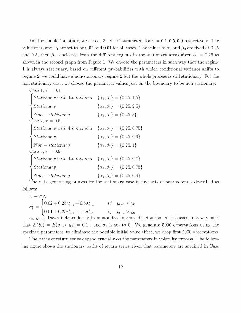
For the simulation study, we choose 3 sets of parameters for π = 0.1, 0.5, 0.9 respectively. Thevalue of ω0 and ω1 are set to be 0.02 and 0.01 for all cases. The values of α0 and β0 are fixed at 0.25and 0.5, then β1 is selected from the different regions in the stationary areas given α1 = 0.25 asshown in the second graph from Figure 1. We choose the parameters in such way that the regime1 is always stationary, based on different probabilities with which conditional variance shifts toregime 2, we could have a non-stationary regime 2 but the whole process is still stationary. For thenon-stationary case, we choose the parameter values just on the boundary to be non-stationary.
Case 1, π = 0.1:Stationary with 4th moment {α1, β1} = {0.25, 1.5}
Stationary {α1, β1} = {0.25, 2.5}
Non− stationary {α1, β1} = {0.25, 3}Case 2, π = 0.5:Stationary with 4th moment {α1, β1} = {0.25, 0.75}
Stationary {α1, β1} = {0.25, 0.9}
Non− stationary {α1, β1} = {0.25, 1}Case 3, π = 0.9:Stationary with 4th moment {α1, β1} = {0.25, 0.7}
Stationary {α1, β1} = {0.25, 0.75}
Non− stationary {α1, β1} = {0.25, 0.9}The data generating process for the stationary case in first sets of parameters is described as
follows:rt = σtεt
σ2t =
0.02 + 0.25r2t−1 + 0.5σ2
t−1 if yt−1 ≤ y0
0.01 + 0.25r2t−1 + 1.5σ2
t−1 if yt−1 > y0
εt, yt is drawn independently from standard normal distribution, y0 is chosen in a way suchthat E(St) = E(yt > y0) = 0.1 , and σ0 is set to 0. We generate 5000 observations using thespecified parameters, to eliminate the possible initial value effect, we drop first 2000 observations.
The paths of return series depend crucially on the parameters in volatility process. The follow-ing figure shows the stationary paths of return series given that parameters are specified in Case
12

1.5
Figure 2: Simulated Paths of the Return Series under Threshold GARCH model
0 500 1000 1500 2000 2500 3000−2.5
−2
−1.5
−1
−0.5
0
0.5
1
1.5
2
2.5stationary return series with fourth moment
3.3 The Performance of MLE Estimator
In this section we examine the performance of maximum likelihood estimator. Given that thereturn series is conditionally normally distributed, the log likelihood function for a sample of Tobservations is:
lnLT (θ) = −1/2T∑
t=1
lnσ2t − 1/2
T∑t=1
r2t
σ2t
where θ = {ω0, ω1, α0, α1, β0, β1}. We know that to estimate θ, we need to estimate the thresholdvalue y0 so that the above likelihood function can be formulated. Here we estimate y0 by gridsearch, the threshold variable yt is sorted and for each possible threshold value y0 we calculatethe corresponding likelihood and the estimated threshold value is the one which maximizes thelikelihood:
5The parameters used in the simulated path are: π = 0.1 {ω0, α0, β0} = {0.02, 0.25, 0.5} {ω1, α1, β1} ={0.01, 0.25, 1.5}
13

θ̂(y0) = argmaxT−1lnL
The asymptotic theory for the maximum likelihood estimates of the parameters of the thresholdGARCH model gives rise to difficulties because of the non-differentiability due to the threshold.Therefore we conduct a simulation study to analyze the finite sample properties of the maximumlikelihood estimator.
Firstly, we present the estimation results for 3 sets of parameters in Case 1 when π = 0.1,considering the sample sizes for 500, 1000, and 2000. The MSE is defined as mean squared errors
of estimates from true parameter values MSE =1
T
∑(θ̂− θ)2 for θ = {ω0, ω1, α0, α1, β0, β1}. The
results are based on 1000 replications. For simplicity we estimate the threshold value by searchingover the 19 grid points range from 5% percentile to 95% percentile points of threshold variable.
Table 1: The MLE estimates for parameters in Case 1Par True
ValueEstimate MSE True
ValueEstimate MSE True
ValueEstimate MSE
ω0 0.02 .0210 .0001 0.02 .0209 .0000 0.02 .0205 .0001ω1 0.01 .0072 .0045 0.01 .0096 .0077 0.01 .0114 .0094
T=500 α0 0.25 .2389 .0076 0.25 .2487 .0051 0.25 .2508 .0077α1 0.25 .2711 .1194 0.25 .3077 .2158 0.25 .3356 .2801β0 0.5 .4905 .0232 0.5 .4908 .0077 0.5 .4725 .0136β1 1.5 1.4712 .8277 2.5 2.3337 1.0359 3 2.6001 1.5691ω0 0.02 .0206 .0000 0.02 .0204 .0000 0.02 .0238 .0131ω1 0.01 .0097 .0015 0.01 .0107 .0025 0.01 .0136 .0032
T=1000 α0 0.25 .2474 .0021 0.25 .2527 .0023 0.25 .2555 .0045α1 0.25 .2569 .0464 0.25 .2843 .0880 0.25 .3160 .1246β0 0.5 .4949 .0042 0.5 .4929 .0037 0.5 .4776 .0093β1 1.5 1.4762 .2526 2.5 2.3752 .4346 3 2.6380 .9153ω0 0.02 .0202 .0000 0.02 .0200 .0000 0.02 .0196 .0000ω1 0.01 .0094 .0007 0.01 .0100 .0012 0.01 .0127 .0018
T=2000 α0 0.25 .2479 .0011 0.25 .2513 .0016 0.25 .2525 .0038α1 0.25 .2519 .0185 0.25 .2700 .0376 0.25 .2910 .0568β0 0.5 .4993 .0022 0.5 .4952 .0031 0.5 .4780 .0096β1 1.5 1.4917 .1096 2.5 2.4091 .2396 3 2.6786 .6989
Table 1 presents the estimation results for 3 sets of parameters in Case 1. When π = 0.1, since
14

the probability that the conditional variance changes to regime 2 is small, we just need the sum ofparameters to be less than 3.25 to fulfill the requirement for stationary distribution. In all 3 setsof parameters, whether they are strict stationary with finite fourth moment, strict stationary, ornon-stationary, the MLE estimator appears to converge to the true parameter value since the themean values of the estimates approach to the true parameter values when the sample size increasesfrom 500 to 2000. The MSE decreases when sample size increases. We notice that the MSE forα1 and β1 are substantially larger then that of α0 and β0, this may be caused by the nature ofnon-stationarity in the corresponding regime and small probability to enter that regime.
Figure 3-5 provide the estimated density of MLE estimates summarized in the above table.The estimated density is computed using kernel smoothing method. The MLE estimates areapproximately unbiased and consistent even the stationarity condition is violated. As sample sizeincreases from 500 to 2000, the MLE estimates become more efficient with smaller variances andmore concentrated around true parameters. We present the density estimates for sample size of500, 1000, and 2000 in dotted line, dashed line, and dotted and dashed line respectively, while thetrue parameter values are given by the solid line.
15

Figure 3: Kernel Smoothing Density Estimates of MLE for Stationary Returns with Fourth Mo-ment when π = 0.1
−0.05 0 0.05 0.10
20
40
60
80
100
120
140
estimates
Kernal Smoothing Density Estimates of MLE ω1 when π=0.1
Sample Size 500Sample Size 1000Sample Size 2000True Value
−0.4 −0.3 −0.2 −0.1 0 0.1 0.2 0.3 0.40
2
4
6
8
10
12
14
16
estimates
Kernal Smoothing Density Estimates of MLE ω2 when π=0.1
−0.4 −0.3 −0.2 −0.1 0 0.1 0.2 0.3 0.4 0.5 0.60
2
4
6
8
10
12
estimates
Kernal Smoothing Density Estimates of MLE α1 when π=0.1
−1 −0.5 0 0.5 1 1.5 2 2.50
0.5
1
1.5
2
2.5
3
estimates
Kernal Smoothing Density Estimates of MLE α2 when π=0.1
−0.2 0 0.2 0.4 0.6 0.8 1 1.2 1.40
1
2
3
4
5
6
7
8
9
10
estimates
Kernal Smoothing Density Estimates of MLE β1 when π=0.1
−3 −2 −1 0 1 2 3 4 5 6 70
0.2
0.4
0.6
0.8
1
1.2
estimates
Kernal Smoothing Density Estimates of MLE β2 when π=0.1
16

Figure 4: Kernel Smoothing Density Estimates of MLE for Stationary Returns without FourthMoment when π = 0.1
−0.01 0 0.01 0.02 0.03 0.04 0.05 0.060
20
40
60
80
100
120
140
160
estimates
Kernal Smoothing Density Estimates of MLE ω1 when π=0.1
Sample Size 500Sample Size 1000Sample Size 2000True Value
−0.4 −0.2 0 0.2 0.4 0.6 0.80
2
4
6
8
10
12
estimates
Kernal Smoothing Density Estimates of MLE ω2 when π=0.1
−0.1 0 0.1 0.2 0.3 0.4 0.5 0.6 0.70
2
4
6
8
10
12
estimates
Kernal Smoothing Density Estimates of MLE α1 when π=0.1
−1.5 −1 −0.5 0 0.5 1 1.5 2 2.5 3 3.50
0.5
1
1.5
2
estimates
Kernal Smoothing Density Estimates of MLE α2 when π=0.1
−0.2 0 0.2 0.4 0.6 0.8 10
2
4
6
8
10
12
estimates
Kernal Smoothing Density Estimates of MLE β1 when π=0.1
−1 0 1 2 3 4 5 6 7 80
0.1
0.2
0.3
0.4
0.5
0.6
0.7
0.8
0.9
1
estimates
Kernal Smoothing Density Estimates of MLE β2 when π=0.1
17

Figure 5: Kernel Smoothing Density Estimates of MLE for Non-Stationary Returns when π = 0.1
−0.02 0 0.02 0.04 0.06 0.08 0.10
20
40
60
80
100
120
140
160
estimates
Kernal Smoothing Density Estimates of MLE ω1 when π=0.1
Sample Size 500Sample Size 1000Sample Size 2000True Value
−0.5 −0.4 −0.3 −0.2 −0.1 0 0.1 0.2 0.3 0.4 0.50
1
2
3
4
5
6
7
8
9
10
11
estimates
Kernal Smoothing Density Estimates of MLE ω2 when π=0.1
−0.1 0 0.1 0.2 0.3 0.4 0.5 0.6 0.7 0.8 0.90
2
4
6
8
10
12
estimates
Kernal Smoothing Density Estimates of MLE α1 when π=0.1
−2 −1 0 1 2 3 40
0.2
0.4
0.6
0.8
1
1.2
1.4
1.6
1.8
2
estimates
Kernal Smoothing Density Estimates of MLE α2 when π=0.1
0.1 0.2 0.3 0.4 0.5 0.6 0.7 0.8 0.90
2
4
6
8
10
12
estimates
Kernal Smoothing Density Estimates of MLE β1 when π=0.1
−2 −1 0 1 2 3 4 5 6 7 8 90
0.1
0.2
0.3
0.4
0.5
0.6
0.7
0.8
estimates
Kernal Smoothing Density Estimates of MLE β2 when π=0.1
Similar results are obtained for other 2 cases and reported in Appendix B. Table 5 presentsthe estimation results for 3 sets of parameters in Case 2. MLE estimators are still consistent andefficient as sample size increases. We also observe that the MSE of estimates in each regime arenot substantially different as reported in Table 1. It may be caused by the fact that probabilitiesof conditional variance in each regime are equal, and we also expect higher MSE for estimates innon-stationary regime. Table 6 presents estimation results in Case 3. When the probability that
18
conditional variance process in regime 2 equals 0.9, even in the stationary case we will no longerhave consistent estimator of β1. Since regime 2 is more volatile regime, here the high probabilitythat the conditional variance is in such regime may be the reason that we fail to get consistentestimator. We also notice that the estimates of parameters in regime 1 turn out to have largerMSE. It confirms our assertion that the small probability in one regime affects the performance ofestimates in that regime. Figure 6-8 provide the estimated density of MLE estimates summarizedin table 2. The MLE estimates are approximately unbiased and consistent even the stationaritycondition is violated. Figure 9-10 provide the estimated density of MLE estimates summarized intable 2.
4 Empirical Study
In this section we apply the threshold model to empirical data and find a good fit of the thresholdGARCH model. We begin with a brief description of the data set and follow with the estimationof the threshold model. Then we discuss the estimation results.
4.1 The Data
The data set consists of 20 stocks in the major market index (MMI)6. We obtain the data of moststocks for the period from Jan. 2, 1970 to Dec. 31, 2008, except for AXP and T. We have data onlystart from May 18, 1977 for AXP and Jan 2, 1984 for T. We choose the stocks from MMI becausethey are well known and highly capitalized stocks representing a broad range of industries andthey generally exhibit a high level of trading activity. Return data are obtained from daily stockfile of the Center for Research in Security Prices (CRSP) and accessed from Wharton ResearchData Services (WRDS).
6The firms in the MMI are American Express (AXP), AT&T (T), Chevron (CHV), Coca-Cola (KO), Disney(DIS), Dow Chemical (DOW), Du Pont (DD), Eastman Kodak (EK), Exxon (XOM), General Electric (GE),General Motors (GM), International Business Machines (IBM), International Paper (IP), Johnson & Johnson (JNJ),McDonald’s (MCD), Merck (MRK), 3M (MMM), Philip Morris (MO), Procter and Gamble (PG), and Sears (S).
19
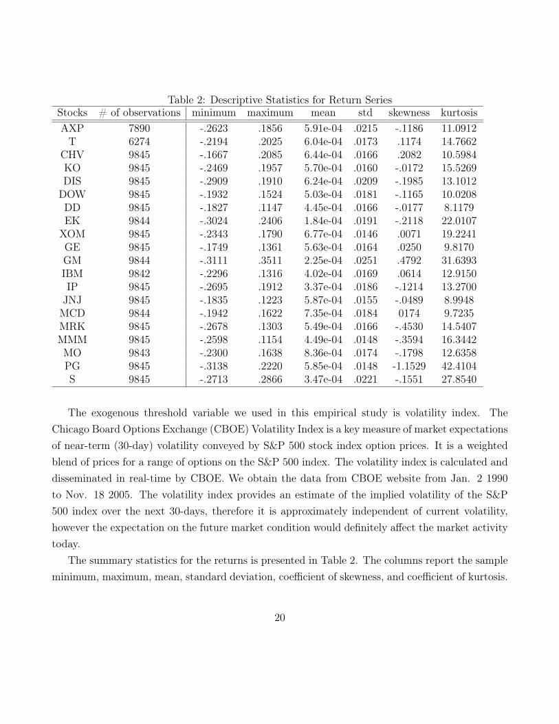
Table 2: Descriptive Statistics for Return SeriesStocks # of observations minimum maximum mean std skewness kurtosisAXP 7890 -.2623 .1856 5.91e-04 .0215 -.1186 11.0912T 6274 -.2194 .2025 6.04e-04 .0173 .1174 14.7662
CHV 9845 -.1667 .2085 6.44e-04 .0166 .2082 10.5984KO 9845 -.2469 .1957 5.70e-04 .0160 -.0172 15.5269DIS 9845 -.2909 .1910 6.24e-04 .0209 -.1985 13.1012DOW 9845 -.1932 .1524 5.03e-04 .0181 -.1165 10.0208DD 9845 -.1827 .1147 4.45e-04 .0166 -.0177 8.1179EK 9844 -.3024 .2406 1.84e-04 .0191 -.2118 22.0107XOM 9845 -.2343 .1790 6.77e-04 .0146 .0071 19.2241GE 9845 -.1749 .1361 5.63e-04 .0164 .0250 9.8170GM 9844 -.3111 .3511 2.25e-04 .0251 .4792 31.6393IBM 9842 -.2296 .1316 4.02e-04 .0169 .0614 12.9150IP 9845 -.2695 .1912 3.37e-04 .0186 -.1214 13.2700JNJ 9845 -.1835 .1223 5.87e-04 .0155 -.0489 8.9948MCD 9844 -.1942 .1622 7.35e-04 .0184 0174 9.7235MRK 9845 -.2678 .1303 5.49e-04 .0166 -.4530 14.5407MMM 9845 -.2598 .1154 4.49e-04 .0148 -.3594 16.3442MO 9843 -.2300 .1638 8.36e-04 .0174 -.1798 12.6358PG 9845 -.3138 .2220 5.85e-04 .0148 -1.1529 42.4104S 9845 -.2713 .2866 3.47e-04 .0221 -.1551 27.8540
The exogenous threshold variable we used in this empirical study is volatility index. TheChicago Board Options Exchange (CBOE) Volatility Index is a key measure of market expectationsof near-term (30-day) volatility conveyed by S&P 500 stock index option prices. It is a weightedblend of prices for a range of options on the S&P 500 index. The volatility index is calculated anddisseminated in real-time by CBOE. We obtain the data from CBOE website from Jan. 2 1990to Nov. 18 2005. The volatility index provides an estimate of the implied volatility of the S&P500 index over the next 30-days, therefore it is approximately independent of current volatility,however the expectation on the future market condition would definitely affect the market activitytoday.
The summary statistics for the returns is presented in Table 2. The columns report the sampleminimum, maximum, mean, standard deviation, coefficient of skewness, and coefficient of kurtosis.
20

4.2 Estimation of the Threshold GARCH model
In this section we apply the threshold GARCH model to the above data set which contains 20stocks from MMI. We assume that the return series follows the threshold GARCH model wherethe volatility index is the exogenous trigger variable.
Since the return series in our threshold GARCH model is assumed to be a zero mean process,we first remove the mean from the returns. In addition to a constant we also filter the AR effectto order 5:
rt = Rt − µ−5∑
j=1
δjRt−j
where Rt is the observed return, µ is the mean, and δj is the coefficient of AR variables.The volatility index is the exogenous trigger in this threshold GARCH model, so we also need
to determine the threshold value for this variable. Now the model that needs to be estimated hasa set of parameters as a function of threshold values.
rt = σtεtσ2t = ω0 + α0r
2t−1 + β0σ
2t−1 if yt−1 ≤ y0
σ2t = ω1 + α1r
2t−1 + β1σ
2t−1 if yt−1 > y0
Define the log likelihood function as follows:
lnLT (θ) = −1/2T∑
t=1
lnσ2t − 1/2
T∑t=1
r2t
σ2t
where θ = {ω0, ω1, α0, α1, β0, β1}. Then the MLE estimator θ̂ is a function of y0:
θ̂(y0) = argmaxT−1lnL
To estimate the threshold value we divide the sample of threshold variable into 40 intervalsand the 39 grid points correspond to 2.5 percentile point to 97.5 percentile point. To evaluate the
21

model performance, we use the Akaike’s information criterion and Bayesian information criterionto compare the threshold GARCH model to standard GARCH (1,1) model.
AIC = 2k − 2lnL
BIC = −2lnL+ kln(n)
where n is the sample size and k is the number of parameters estimated in the model.
4.3 Preliminary Results
The MLE estimates are presented in Table 3.
22

Table 3: The Estimates of Threshold GARCH model Using VIX as Threshold Variable
y0 α0 α1 β0 β1 LLF AIC BICAXP GARCH(1,1) .062
.007.9368
.00712202 -24398 -24379
TS y90 .04140056
.14760289
.95520061
.86430214
12218 -24425 -24393
T GARCH(1,1) .0317.006
.9678.0068
10400 -20794 -20775TS y625 .0530
0111.01420064
.93560110
.98420076
10419 -20828 -20797
CHV GARCH(1,1) .0611.0091
.9209.0118
13590 -27174 -27155TS y60 .0354
0102.08600148
.91480207
.89410167
13607 -27204 -27171
KO GARCH(1,1) .0485.0078
.9490.0079
13672 -27338 -27319TS y925 .0272
0046.13780352
.97040051
.86130309
13694 -27378 -27346
DIS GARCH(1,1) .0555.0114
.9374.0115
12437 -24867 -24848TS y35 .0634
0180.10230278
.74020539
.85150307
12476 -24943 -24911
DOW GARCH(1,1) .0575.0080
.9392.0083
12846 -25686 -25667TS y675 .0523
0112.06200120
.92600132
.93750115
12857 -25704 -25671
DD GARCH(1,1) .0343.0051
.9632.0058
12950 -25894 -25875TS y925 .0247
0005.11860000
.97230002
.87790001
12967 -25924 -25892
EK GARCH(1,1) .1990.0473
.6231.0684
11973 -23940 -23921TS y625 .1290
0552.29690964
.20631375
.46560897
12051 -24092 -24060
XOM GARCH(1,1) .0589.0083
.9302.0094
13768 -27531 -27511TS y95 .0400
0001.18350002
.95210001
.83370002
13787 -27563 -27531
GE GARCH(1,1) .047.0063
.9522.0064
13478 -26950 -26931TS y775 .0179
0041.10190191
.97740047
.90300173
13508 -27006 -26973
GM GARCH(1,1) .0611.0093
.9268.0141
11596 -23186 -23167TS y675 .0352
0067.09160160
.94540120
.90760155
11611 -23212 -23180
IBM GARCH(1,1) .0542.0085
.9434.0089
12641 -25277 -25257TS y925 .0311
0056.21180461
.96640062
.80340317
12662 -25314 -25282
IP GARCH(1,1) .0518.0079
.9419.0083
12643 -25281 -25261TS y575 .0305
0109.12760247
.87130321
.85390235
12680 -25350 -25318
23

Continue of Table 3JNJ GARCH(1,1) .0731
.0101.9235.0096
13807 -27609 -27589TS y85 .0469
0067.13290319
.95130070
.87230225
13819 -27627 27595
MCD GARCH(1,1) .0420.0071
.9513.0080
12998 -25990 -25971TS y60 .0335
0096.04080095
.94000140
.95160097
13014 -26019 -25986
MRK GARCH(1,1) .0411.0128
.9037.0353
12495 -24985 -24966TS y675 .0106
0129.07260234
.91970327
.89470338
12539 -25069 -25036
MMM GARCH(1,1) .0404.0089
.9399.0135
13630 -27255 -27235TS y575 .0316
0193.11550292
.68330734
.78230436
13692 -27373 -27341
MO GARCH(1,1) .0476.0101
.9453.0117
12680 -25353 -25334TS y125 .5050
3010.06700138
.63490933
.90930164
12722 -25435 -25402
PG GARCH(1,1) .0398.0065
.9578.0068
13758 -27510 -27490TS y80 .0172
0044.14960465
.97980046
.86900305
13794 -27578 -27545
S GARCH(1,1) .1051.0228
.8584.0225
9343 -18680 -18662TS y50 .1037
0223.11190369
.78630432
.84710313
9374 -18737 -18706
The parameters in the threshold GARCH model are significant for 19 out of 20 stocks except β1
for EK. The likelihood and the model selection criteria AIC and BIC suggest the better fit of dataof the threshold GARCH model than traditional GARCH model. Since we use the volatility indexas the threshold variable for all 20 stocks, it is possible that some stocks are more sensitive to themarket conditions than others, therefore we observe in some stocks the estimated parameters arevery similar in both regimes. For some stocks we have the sum of estimated parameters greaterthan 1 in one regime, but consider the probability that conditional variance stays in that regime,we will still have the stationary process. The probability is given by the location of the thresholdvalue in the sample space of the threshold variable, it is very clear in our estimation results since weuse 2.5 percentile as the increment. For example the estimated parameters in regime 2 have a sumof 1.0172, but the threshold value estimated is y95, that means there is only 5% of chances that theconditional variance shifts to the regime 2, therefore the stationarity conditions still hold. Thoughthis simple empirical exercise is not sufficient proof of the threshold GARCH model, it provides aperspective of the further exploration and application of such a simple but flexible model.
24
5 Conclusion
In this paper we define a threshold GARCH model with exogenous triggers to describe theconditional variance dynamics. This model can capture both the regime-switching feature andthe effect of exogenous variables such as volatility index on the regime shifts of the conditionalvariance process. The model is flexible to accommodate other exogenous variables that can triggerthe regime changes. Although the theoretical asymptotic distribution of the estimator is hard toestablish, we show by simulation that the MLE estimator is approximately unbiased and consistent.The model is also applied to the data set with 20 stocks, the performance of the model is comparedwith standard GARCH (1,1) model and showed good fit of the data.
25

Appendix A
Proof of Proposition 1
We rewrite the conditional variance equation as:
σ2t =ω0(1− St−1) + ω1St−1 + (α0(1− St−1) + α1St−1)r
2t−1 + (β0(1− St−1) + β1St−1)σ
2t−1
= ω0 + (ω1 − ω0)St−1 + [(α0 + (α1 − α0)St−1)ε2t−1 + β0 + (β1 − β0)St−1]σ
2t−1 (1)
Let
c0 = ω0(1− π) + ω1π c1 = ω1 − ω0
a0 = α0(1− π) + α1π a1 = α1 − α0
b0 = β0(1− π) + β1π b1 = β1 − β0
Bt = St − π
Then (1) can be rewritten as:
σ2t = c0 + c1Bt−1 + [ε2
t−1(a0 + a1Bt−1) + b0 + b1Bt−1]σ2t−1 (2)
The transformation makes the random variables in the coefficient have mean zero. Back sub-stitution in (2) results in:
σ2t = c0 + c1Bt−1 +
k−1∑n=1
(c0 + c1Bt−1−n)n∏
m=1
[ε2t−m(a0 + a1Bt−m) + b0 + b1Bt−m]
+k∏
m=1
[ε2t−m(a0 + a1Bt−m) + b0 + b1Bt−m]σ2
t−k
Let we define Sn(t) as:
Sn(t) =n∏
m=1
[ε2t−m(a0 + a1Bt−m) + b0 + b1Bt−m]
26

Then we have1
nln(Sn(t))
a.s.−→ E(ln[ε2t−m(a0 + a1Bt−m) + b0 + b1Bt−m])
It’s very clear that if E(ln[ε2t−m(a0 + a1Bt−m) + b0 + b1Bt−m]) < 0 , that is [(α0 + β0)(1− π) +
(α1 + β1)π] < 1, then the terms Sn(t) are geometrically bounded as n increases and equation (2)has the solution:
σ2t = c0 + c1Bt−1 +
∞∑n=1
(c0 + c1Bt−1−n)Sn(t) (3)
Therefore the return process has a stationary solution given by:
rt =
√c0 + c1Bt−1 +
∞∑n=1
(c0 + c1Bt−1−n)Sn(t)εt .
Proof of Proposition 2
Taking expectation on both side of equation (3) we have:
E(σ2t ) = E(c0 + c1Bt−1) +
∞∑n=1
E(c0 + c1Bt−1−n)E(Sn(t)) (4)
Given that εt and St are independent, we have:
E(Sn(t)) = E[n∏
m=1
(ε2t−m(a0 + a1Bt−m) + b0 + b1Bt−m)]
=n∏
m=1
[E(ε2t−m(a0 + a1Bt−m)) + E(b0 + b1Bt−m)]
= (a0 + b0)n
Provided that a0 + b0 < 1, that is (α0 + β0)(1− π) + (α1 + β1)π < 1, the equation (4) becomes:
27

E(σ2t ) = E(c0 + c1Bt−1) +
∞∑n=1
E(c0 + c1Bt−1−n)E(Sn(t))
= c0 + c0
∞∑n=1
(a0 + b0)n
= c0
∞∑n=0
(a0 + b0)n
=c0
1− (a0 + b0)
=ω0(1− π) + ω1π
1− [(α0 + β0)(1− π) + (α1 + β1)π]
Proof of Proposition 3
To examine the stationarity conditions for higher order moments of return, we check the secondmoment of σ2
t :
E(σ4t ) = E[(c0 + c1Bt−1) +
∞∑n=1
(c0 + c1Bt−1−n)Sn(t)]2
= E(c0 + c1Bt−1)2 + E[2(c0 + c1Bt−1)
∞∑n=1
(c0 + c1Bt−1−n)Sn(t)] + E[∞∑
n=1
(c0 + c1Bt−1−n)Sn(t)]2
= c20 + c21π(1− π) + 2c20
∞∑n=1
E(Sn(t)) + 2c0c1
∞∑n=1
E(Bt−1−nSn(t)) + 2c0c1
∞∑n=1
E(Bt−1Sn(t))
+2c21E[Bt−1
∞∑n=1
Bt−1−nSn(t)] + E[∞∑
n=1
(c0 + c1Bt−1−n)Sn(t)]2
Note that
28

E(Bt−1Sn(t)) = E{Bt−1[ε2t−1(a0 + a1Bt−1) + b0 + b1Bt−1]Sn(t− 1)}
= (a1 + b1)π(1− π)(a0 + b0)n−1
E[∞∑
n=1
(c0 + c1Bt−1−n)Sn(t)]2 = E[c0
∞∑n=1
Sn(t) + c1
∞∑n=1
Bt−1−nSn(t)]2
= E[c20(∞∑
n=1
Sn(t))2] + E[2c0c1
∞∑n=1
Sn(t)∞∑
n=1
Bt−1−nSn(t)]
+E[c1
∞∑n=1
Bt−1−nSn(t)]2
E[c20(∞∑
n=1
Sn(t))2] = c20[∞∑
n=1
E(S2n(t)) + 2
∞∑n=1
∞∑l=n+1
E(Sn(t)Sl(t)]
E[2c0c1
∞∑n=1
Sn(t)∞∑
n=1
Bt−1−nSn(t)] = 0
E[c1
∞∑n=1
Bt−1−nSn(t)]2 = c21[π(1− π)∞∑
n=1
E(S2n(t))
+2∞∑
n=1
∞∑l=n+1
E(Bt−1−nBt−1−lSn(t)Sl(t)]
where
29

E(S2n(t)) = E
n∏m=1
(ε2t−m(a0 + a1Bt−m) + b0 + b1Bt−m)2
= E
n∏m=1
[ε4t−m(a0 + a1Bt−m)2 + 2ε2
t−m(a0 + a1Bt−m)(b0 + b1Bt−m)
+(b0 + b1Bt−m)2]
= [3a20 + a2
1π(1− π) + 2a0b0 + 2a1b1π(1− π) + b20 + b21π(1− π)]n
= [2a20 + (a0 + b0)
2 + (2a21 + (a1 + b1)
2)π(1− π)]n
Let A = 2a20 + (a0 + b0)
2 + (2a21 + (a1 + b1)
2)π(1− π) , then
E(Sn(t)Sl(t) = E[n∏
m=1
(ε2t−m(a0 + a1Bt−m) + b0 + b1Bt−m)2
∞∏m=n+1
(ε2t−m(a0 + a1Bt−m) + b0 + b1Bt−m)]
= An(a0 + b0)l−n
Therefore:
E[c20(∞∑
n=1
Sn(t))2] = c20(∞∑
n=1
An + 2∞∑
n=1
∞∑l=n+1
An(a0 + b0)l−n)
E[c1
∞∑n=1
Bt−1−nSn(t)]2 = c21π(1− π)∞∑
n=1
An
Provided that
A = 2a20 + (a0 + b0)
2 + (2a21 + (a1 + b1)
2)π(1− π)
= (2α20 + (α0 + β0)
2)(1− π) + (2α21 + (α1 + β1)
2)π < 1
30

The above equations can be simplified as:
E[c20(∞∑
n=1
Sn(t))2] = c20(∞∑
n=1
An(1 + 2∞∑
j=1
(a0 + b0)j))
= c20A(1 + (a0 + b0))
(1− A)(1− (a0 + b0))
E[c1
∞∑n=1
Bt−1−nSn(t)]2 = c21π(1− π)∞∑
n=1
An
= c21π(1− π)A
(1− A)
Substitute back to the expression of E(σ4t ), we have:
E(σ4t ) = c20 + c21π(1− π) + 2c20
∞∑n=1
(a0 + b0)n + 2c0c1π(1− π)(a1 + b1)
∞∑n=1
(a0 + b0)n−1
+c20A(1 + a0 + b0)
(1− A)(1− (a0 + b0))+ c21π(1− π)
A
(1− A)
= c20 + c21π(1− π) +2c20(a0 + b0)
1− (a0 + b0)+ 2c0c1π(1− π)
a1 + b11− (a0 + b0)
+c20A(1 + a0 + b0)
(1− A)(1− (a0 + b0))+ c21π(1− π)
A
(1− A)
= c201 + a0 + b0
(1− A)(1− (a0 + b0))+ c1π(1− π)
c1(1− (a0 + b0)) + 2c0(a1 + b1)(1− A)
(1− A)(1− (a0 + b0)
Proof of Proposition 4
We have σ2 = E(r2t ) =
c01− (a0 + b0)
, subtract mean from equation (2), we get:
31

σ2t − σ2 = c1Bt−1 + [ε2
t−1(a0 + a1Bt−1) + b0 + b1Bt−1]σ2t−1 − σ2(a0 + b0)
= c1Bt−1 + (a0 + a1Bt−1)r2t−1 + (b0 + b1Bt−1)σ
2t−1 − σ2(a0 + b0)
r2t − σ2 = c1Bt−1 + (a0 + a1Bt−1)r
2t−1 + (b0 + b1Bt−1)σ
2t−1 − σ2(a0 + b0)− ht + r2
t
= [a0 + b0 + (a1 + b1)Bt−1](r2t−1 − σ2) + (σ2(a1 + b1) + c1)Bt−1
−(b0 + b1Bt−1)(r2t−1 − σ2
t−1) + r2t − σ2
t
= [a0 + b0 + (a1 + b1)Bt−1](r2t−1 − σ2) + (σ2(a1 + b1) + c1)Bt−1
σ2t (ε
2t − 1)− (b0 + b1Bt−1)σ
2t−1(ε
2t−1 − 1)
The above expression of r2t − σ2 is very similar to the equation (3.6) in Ding and Granger
(1996). Interestingly, the above expression represents r2t −σ2 as an random coefficient ARMA(1,1)
process if we write the compound error as an MA(1) process; letting σ2t (ε
2t − 1) = vt:
σ2t (ε
2t − 1)− (b0 + b1Bt−1)σ
2t−1(ε
2t−1 − 1) = vt − (b0 + b1Bt−1)vt−1
with E(vt) = 0 and E(vtvs) = 0 for all t 6= s . Therefore, without any formal proof, theinformation already gives us some idea of the behaviors of the auto covariances.
Multiply both sides by (r2t−1 − σ2):
(r2t − σ2)(r2
t−1 − σ2) = [a0 + b0 + (a1 + b1)Bt−1](r2t−1 − σ2)2 + (σ2(a1 + b1) + c1)Bt−1(r
2t−1 − σ2)
−(b0 + b1Bt−1)(r2t−1 − σ2
t−1)(r2t−1 − σ2) + (r2
t − σ2t )(r
2t−1 − σ2)
Taking expectation on both sides
E(r2t − σ2)(r2
t−1 − σ2) = (a0 + b0)E(r2t−1 − σ2)2 − b0E(r2
t−1 − σ2t−1)(r
2t−1 − σ2)
+E(r2t − σ2
t )(r2t−1 − σ2)
γ(1) = (a0 + b0)γ(0)− 2b0E(σ4t−1)
32
where γ(1) = E(r2t −σ2)(r2
t−1−σ2) is the covariance between r2t and r2
t−1, and γ(0) = E(r2t−1−
σ2)2 is the variance of r2t−1. If we assume that the second moment of conditional variance or the
fourth moment of residual exists, that is when the conditions in proposition 3 satisfied, then it canbe shown that:
ρ(1) =c20[2a0 − 2a0b0A0 + A0(2a
21 + (a1 + b1)
2)π(1− π)]
c20(2 + A− 3A20) + 3c1π(1− π)[c1(1− A0) + 2c0(a1 + b1)(1− A)]
+(3a0 + b0(1 + 2A0))π(1− π)[c21 + 2c0c1(a1 + b1)(1− A)]
c20(2 + A− 3A20) + 3c1π(1− π)[c1(1− A0) + 2c0(a1 + b1)(1− A)]
where A0 = a0 + b0
It is easy to show that:
γ(k) = (a0 + b0)γ(k − 1) for k ≥ 2, and ρ(k) = (a0 + b0)k−1ρ(1)
33

Appendix B
Table 5: The MLE estimates for parameters in Case 2Par True
ValueEstimate MSE True
ValueEstimate MSE True
ValueEstimate MSE
ω0 0.02 .0229 .0005 0.02 .0226 .0003 0.02 .0201 .0002ω1 0.01 .0090 .0010 0.01 .0096 .0005 0.01 .0107 .0004
T=500 α0 0.25 .2342 .0192 0.25 .2383 .0081 0.25 .2243 .0111α1 0.25 .2415 .0313 0.25 .2370 .0123 0.25 .2265 .0183β0 0.5 .4768 .0649 0.5 .4880 .0159 0.5 .4546 .0291β1 0.75 .7973 .1577 0.9 .9314 .0439 1 .9020 .1091ω0 0.02 .0212 .0002 0.02 .0209 .0001 0.02 .0194 .0001ω1 0.01 .0093 .0003 0.01 .0103 .0001 0.01 .0103 .0001
T=1000 α0 0.25 .2482 .0092 0.25 .2463 .0024 0.25 .2307 .0074α1 0.25 .2477 .0096 0.25 .2483 .0044 0.25 .2364 .0096β0 0.5 .4811 .0375 0.5 .4949 .0042 0.5 .4611 .0235β1 0.75 .7740 .0509 0.9 .9063 .0085 1 .8962 .0914ω0 0.02 .0207 .0001 0.02 .0204 .0000 0.02 .0203 .0000ω1 0.01 .0096 .0001 0.01 .0101 .0000 0.01 .0107 .0001
T=2000 α0 0.25 .2487 .0023 0.25 .2482 .0011 0.25 .2567 .0015α1 0.25 .2473 .0030 0.25 .2477 .0018 0.25 .2599 .0027β0 0.5 .4897 .0090 0.5 .4987 .0018 0.5 .5050 .0021β1 0.75 .7651 .0152 0.9 .9012 .0033 1 .9754 .0061
34
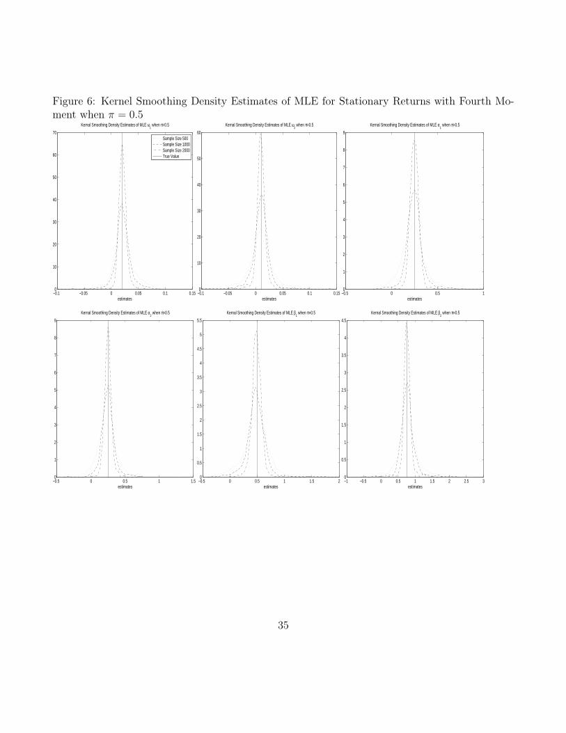
Figure 6: Kernel Smoothing Density Estimates of MLE for Stationary Returns with Fourth Mo-ment when π = 0.5
−0.1 −0.05 0 0.05 0.1 0.150
10
20
30
40
50
60
70
estimates
Kernal Smoothing Density Estimates of MLE ω1 when π=0.5
Sample Size 500Sample Size 1000Sample Size 2000True Value
−0.1 −0.05 0 0.05 0.1 0.150
10
20
30
40
50
60
estimates
Kernal Smoothing Density Estimates of MLE ω2 when π=0.5
−0.5 0 0.5 10
1
2
3
4
5
6
7
8
9
estimates
Kernal Smoothing Density Estimates of MLE α1 when π=0.5
−0.5 0 0.5 1 1.50
1
2
3
4
5
6
7
8
9
estimates
Kernal Smoothing Density Estimates of MLE α2 when π=0.5
−0.5 0 0.5 1 1.5 20
0.5
1
1.5
2
2.5
3
3.5
4
4.5
5
5.5
estimates
Kernal Smoothing Density Estimates of MLE β1 when π=0.5
−1 −0.5 0 0.5 1 1.5 2 2.5 30
0.5
1
1.5
2
2.5
3
3.5
4
4.5
estimates
Kernal Smoothing Density Estimates of MLE β2 when π=0.5
35
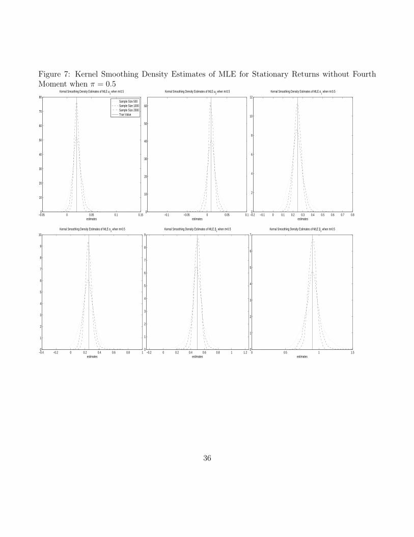
Figure 7: Kernel Smoothing Density Estimates of MLE for Stationary Returns without FourthMoment when π = 0.5
−0.05 0 0.05 0.1 0.150
10
20
30
40
50
60
70
80
estimates
Kernal Smoothing Density Estimates of MLE ω1 when π=0.5
Sample Size 500Sample Size 1000Sample Size 2000True Value
−0.1 −0.05 0 0.05 0.10
10
20
30
40
50
60
estimates
Kernal Smoothing Density Estimates of MLE ω2 when π=0.5
−0.2 −0.1 0 0.1 0.2 0.3 0.4 0.5 0.6 0.7 0.80
2
4
6
8
10
12
estimates
Kernal Smoothing Density Estimates of MLE α1 when π=0.5
−0.4 −0.2 0 0.2 0.4 0.6 0.8 10
1
2
3
4
5
6
7
8
9
10
estimates
Kernal Smoothing Density Estimates of MLE α2 when π=0.5
−0.2 0 0.2 0.4 0.6 0.8 1 1.20
1
2
3
4
5
6
7
8
9
estimates
Kernal Smoothing Density Estimates of MLE β1 when π=0.5
0 0.5 1 1.50
1
2
3
4
5
6
7
estimates
Kernal Smoothing Density Estimates of MLE β2 when π=0.5
36

Figure 8: Kernel Smoothing Density Estimates of MLE for Non-Stationary Returns when π = 0.5
−0.06 −0.04 −0.02 0 0.02 0.04 0.06 0.08 0.1 0.120
10
20
30
40
50
60
70
estimates
Kernal Smoothing Density Estimates of MLE ω1 when π=0.5
Sample Size 500Sample Size 1000Sample Size 2000True Value
−0.1 −0.05 0 0.05 0.1 0.150
5
10
15
20
25
30
35
40
45
50
55
estimates
Kernal Smoothing Density Estimates of MLE ω2 when π=0.5
−0.2 0 0.2 0.4 0.6 0.8 10
2
4
6
8
10
12
estimates
Kernal Smoothing Density Estimates of MLE α1 when π=0.5
−0.2 0 0.2 0.4 0.6 0.8 1 1.20
1
2
3
4
5
6
7
8
9
estimates
Kernal Smoothing Density Estimates of MLE α2 when π=0.5
0 0.1 0.2 0.3 0.4 0.5 0.6 0.7 0.8 0.90
2
4
6
8
10
12
estimates
Kernal Smoothing Density Estimates of MLE β1 when π=0.5
0.4 0.6 0.8 1 1.2 1.4 1.6 1.8 20
1
2
3
4
5
6
7
estimates
Kernal Smoothing Density Estimates of MLE β2 when π=0.5
37

Table 6: MLE Estimates of Parameters in Case 3Par True
ValueEstimate MSE True
ValueEstimate MSE
ω0 0.02 .0175 .0007 0.02 .0210 .0009ω1 0.01 .0118 .0007 0.01 .0123 .0010
T=500 α0 0.25 .2361 .0257 0.25 .2353 .0215α1 0.25 .2437 .0304 0.25 .2412 .0236β0 0.5 .5780 .0973 0.5 .5562 .0528β1 0.7 .7088 .0988 0.75 .7505 .0658ω0 0.02 .0179 .0003 0.02 .0185 .0004ω1 0.01 .0104 .0002 0.01 .0112 .0002
T=1000 α0 0.25 .2482 .0143 0.25 .2444 .0124α1 0.25 .2501 .0119 0.25 .2491 .0080β0 0.5 .5543 .0472 0.5 .5452 .0349β1 0.7 .7075 .0352 0.75 .7425 .0200ω0 0.02 .0180 .0002 0.02 .019 .0002ω1 0.01 .0099 .0001 0.01 .0103 .0001
T=2000 α0 0.25 .2510 .0069 0.25 .2488 .0051α1 0.25 .2489 .0040 0.25 .2475 .0019β0 0.5 .5434 .0264 0.5 .5251 .0156β1 0.7 .7086 .0151 0.75 .7503 .0060
38

Figure 9: Kernel Smoothing Density Estimates of MLE for Stationary Returns with Fourth Mo-ment when π = 0.9
−0.1 −0.05 0 0.05 0.1 0.15 0.20
5
10
15
20
25
30
35
40
45
50
estimates
Kernal Smoothing Density Estimates of MLE ω1 when π=0.9
Sample Size 500Sample Size 1000Sample Size 2000True Value
−0.1 −0.05 0 0.05 0.1 0.150
10
20
30
40
50
60
70
80
90
estimates
Kernal Smoothing Density Estimates of MLE ω2 when π=0.9
−0.5 0 0.5 10
1
2
3
4
5
6
estimates
Kernal Smoothing Density Estimates of MLE α1 when π=0.9
−0.5 0 0.5 1 1.50
1
2
3
4
5
6
7
8
9
estimates
Kernal Smoothing Density Estimates of MLE α2 when π=0.9
−1 0 1 2 3 4 50
0.5
1
1.5
2
2.5
3
estimates
Kernal Smoothing Density Estimates of MLE β1 when π=0.9
−0.5 0 0.5 1 1.5 2 2.50
1
2
3
4
5
6
7
estimates
Kernal Smoothing Density Estimates of MLE β2 when π=0.9
39

Figure 10: Kernel Smoothing Density Estimates of MLE for Stationary Returns without FourthMoment when π = 0.9
−0.1 −0.05 0 0.05 0.1 0.15 0.20
5
10
15
20
25
30
35
estimates
Kernal Smoothing Density Estimates of MLE ω1 when π=0.9
Sample Size 500Sample Size 1000Sample Size 2000True Value
−0.1 −0.05 0 0.05 0.1 0.150
20
40
60
80
100
120
estimates
Kernal Smoothing Density Estimates of MLE ω2 when π=0.9
−0.5 0 0.5 10
1
2
3
4
5
6
estimates
Kernal Smoothing Density Estimates of MLE α1 when π=0.9
−0.5 0 0.5 10
2
4
6
8
10
12
estimates
Kernal Smoothing Density Estimates of MLE α2 when π=0.9
−1 −0.5 0 0.5 1 1.50
0.5
1
1.5
2
2.5
3
3.5
estimates
Kernal Smoothing Density Estimates of MLE β1 when π=0.9
−0.5 0 0.5 1 1.50
2
4
6
8
10
12
estimates
Kernal Smoothing Density Estimates of MLE β2 when π=0.9
40

References[1] Andersen, T. G. (1996), “Return Volatility and Trading Volume: An Information Flow Inter-
pretation of Stochastic Volatility,” Journal of Finance, 51, 169-204.
[2] Bollerslev, T. (1986), “Generalized Autoregressive Conditional Heteroskadasticity,” Journal ofEconometrics, 31, 307-327.
[3] Bollerslev, T., Chou, R. Y., and Kroner, K. F. (1992), “ARCH Modeling in Finance: A Reviewof the Theory and Empirical Evidence,” Journal of Econometrics, 52, 5-59.
[4] Bollerslev, T., and Jubinski, P. D. (1999), “Equity Trading Volume and Volatility: Latent In-formation Arrivals and Common Long-Run Dependencies,” Journal of Business and EconomicStatistics, 17, 9-21.
[5] Clark, P. K. (1973), “A Subordinated Stochastic Process Model with Finite Variance forSpeculative Prices,” Econometrica, 41, 135-155.
[6] Ding, Z., and Granger, C. W. J. (1996), “Modeling Volatility Persistence of Speculative Re-turns: A New Approach,” Journal of Econometrics, 73, 185-215.
[7] Engle, R. F. (1982), “Autoregressive Conditional Heteroskedasticity with Estimates of theVariance of U.K. Inflation,” Econometrica, 50, 987-1008.
[8] Epps, T., and Epps, M. (1976), “The Stochastic Dependence of Security Price Changes andTransaction Volumes: Implications for the Mixture-of-Distribution Hypothesis,” Economet-rica, 44, 305-321.
[9] Gallant, A. R., and Rossi, P. E., and Tauchen, G. (1992), “Stock Prices and Volume,” TheReview of Financial Studies, 5, 199-242.
[10] Glosten, L. R., Jagannathan, R., and Runkle, D. E. (1993), “On the Relation between theExpected Value and the Volatility of the Nominal Excess Return on Stocks,” Journal ofFinance, 48, 1779-1801.
[11] Gray, S. F. (1996), “Modeling the Conditional Distribution of Interest Rates as A Regime-Switching Process,” Journal of Financial Economics, 42, 27-62.
[12] Hamilton, J. D., and Susmel, R. (1994), “Autoregressive Conditional Heteroskedasticity andChanges in Regimes,” Journal of Econometrics, 64, 307-333.
[13] Hansen, P. R., and Lunde, A. (2005), “A Forecast Comparison of Volatility Models: DoesAnything Beat A GARCH (1,1)?” Journal of Applied Econometrics, 20, 873-889.
41

[14] Karpoff, J. M. (1987), “The Relationship between Price Changes and Trading Volume: ASurvey,” Journal of Financial and Quantitative Analysis, 22, 109-126
[15] Klivecka, A. (2004), “Random Coefficient GARCH(1,1) Model with IID Coefficients,” Lithua-nian Mathematical Journal, 44, 374-385.
[16] Knight, J., and Satchell, S. E. (2009), “Some New Results for Threshold AR(1) Models”
[17] Kourtellos, A., Stengos, T., and Tan, C. M. (2009), “THRET: Threshold Regression withEndogenous Threshold Variables”
[18] Lamoureux, C. G., and Lastrapes, W. D. (1990), “Heteroskedasticity in Stock Return Data:Volume versus GARCH Effects,” The Journal of Finance, 45, 221-229.
[19] Nelson, D. B. (1991), “Conditional Heteroskedasticity in Asset Pricing: A New Approach,”Econometrica 59, 347-370.
[20] Poon, S., and Granger, C. W. J. (2003), “Forecasting Volatility in Financial Markets: AReview,” Journal of Economic Literature, 41, 478-539.
[21] Quinn, B. G. (1982), “A Note on the Existence of Strictly Stationary Solutions to BilinearEquations,” Journal of Time Series Analysis, 3, 249-252.
[22] Tauchen, G. E., and Pitts, M. (1983), “The Price Variability-Volume Relationship on Specu-lative Markets,” Econometrica, 51, 485-505.
[23] Rabemananjara, R., and Zakoian, J. M. (1993), “Threshold ARCH Models and Asymmetriesin Volatility,” Journal of Applied Econometrics, 8, 31-49.
[24] Wagner, N. F., and Marsh, T. A. (2005), “Surprise Volume and Heteroskedasticity in EquityMarket Returns,” Available at SSRN: http://ssrn.com/abstract=591206
42