marlene marchena marchenamarlene@gmail · outline inventory the basic economic order quantity (eoq)...
TRANSCRIPT
SCperf: An inventory management package for R
Marlene [email protected]
Department of Electrical EngineeringPontifical Catholic University of Rio de Janeiro - Brazil.
Outline
� Inventory
� The basic Economic Order Quantity (EOQ) model� EOQ assumptions� Derivation of the model
� Inventory models
� What is SCperf?
� EOQ() example
� Bullwhip Effect (BE)� Measuring the BE� Measuring the BE for a generalized demand process� SCperf()
� Why did we develop SCperf?
Inventory
� What is inventory?
Stock of items kept to meet future demand
� Why to hold inventory?
To protect himself against irregular supply and demand
� Inventory Control Decisions
Objective: To minimize total inventory cost
Decisions:
� How much to order?� When to order?
Inventory
� What is inventory?
Stock of items kept to meet future demand
� Why to hold inventory?
To protect himself against irregular supply and demand
� Inventory Control Decisions
Objective: To minimize total inventory cost
Decisions:
� How much to order?� When to order?

Inventory
� What is inventory?
Stock of items kept to meet future demand
� Why to hold inventory?
To protect himself against irregular supply and demand
� Inventory Control Decisions
Objective: To minimize total inventory cost
Decisions:
� How much to order?� When to order?
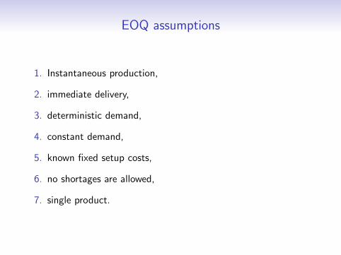
EOQ assumptions
1. Instantaneous production,
2. immediate delivery,
3. deterministic demand,
4. constant demand,
5. known fixed setup costs,
6. no shortages are allowed,
7. single product.
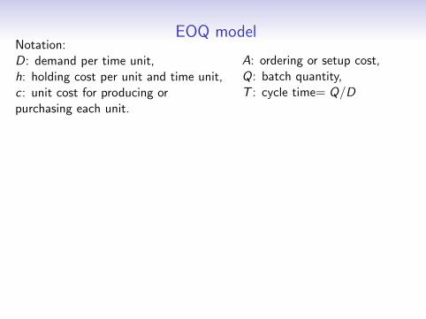
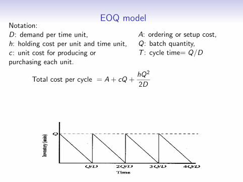
EOQ modelNotation:D: demand per time unit,h: holding cost per unit and time unit,c: unit cost for producing orpurchasing each unit.
A: ordering or setup cost,Q: batch quantity,T : cycle time= Q/D
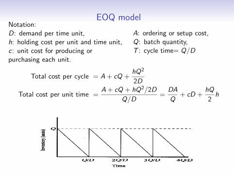
Total cost per cycle = A + cQ +hQ2
2D
Total cost per unit time =A + cQ + hQ2/2D
Q/D=
DA
Q+ cD +
hQ
2h
EOQ modelNotation:D: demand per time unit,h: holding cost per unit and time unit,c: unit cost for producing orpurchasing each unit.
A: ordering or setup cost,Q: batch quantity,T : cycle time= Q/D
Total cost per cycle = A + cQ +hQ2
2D
Total cost per unit time =A + cQ + hQ2/2D
Q/D=
DA
Q+ cD +
hQ
2h
EOQ modelNotation:D: demand per time unit,h: holding cost per unit and time unit,c: unit cost for producing orpurchasing each unit.
A: ordering or setup cost,Q: batch quantity,T : cycle time= Q/D
Total cost per cycle = A + cQ +hQ2
2D
Total cost per unit time =A + cQ + hQ2/2D
Q/D=
DA
Q+ cD +
hQ
2h
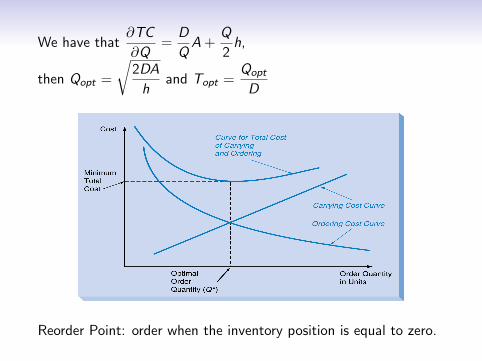
We have that∂TC
∂Q=
D
QA +
Q
2h,
then Qopt =
√2DA
hand Topt =
Qopt
D
Reorder Point: order when the inventory position is equal to zero.
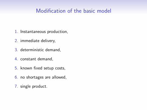
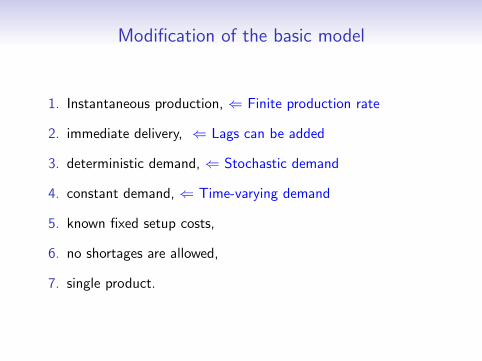
Modification of the basic model
1. Instantaneous production,
⇐ Finite production rate
2. immediate delivery,
⇐ Lags can be added
3. deterministic demand,
⇐ Stochastic demand
4. constant demand,
⇐ Time-varying demand
5. known fixed setup costs,
⇐ Constraint approach
6. no shortages are allowed,
⇐ Shortages are allowed
7. single product.
⇐ Multiple products
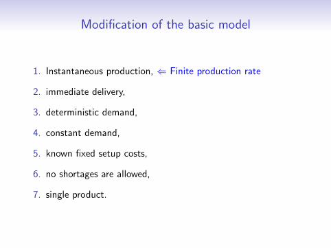
Modification of the basic model
1. Instantaneous production, ⇐ Finite production rate
2. immediate delivery,
⇐ Lags can be added
3. deterministic demand,
⇐ Stochastic demand
4. constant demand,
⇐ Time-varying demand
5. known fixed setup costs,
⇐ Constraint approach
6. no shortages are allowed,
⇐ Shortages are allowed
7. single product.
⇐ Multiple products
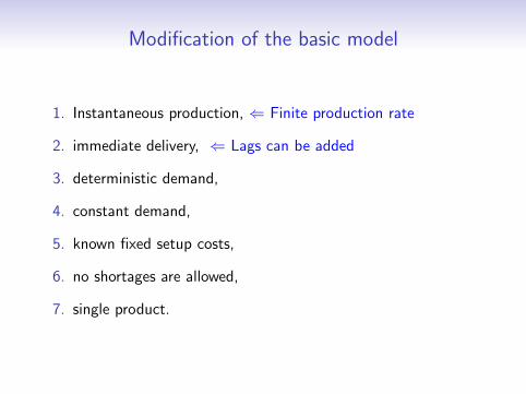
Modification of the basic model
1. Instantaneous production, ⇐ Finite production rate
2. immediate delivery, ⇐ Lags can be added
3. deterministic demand, ⇐ Stochastic demand
4. constant demand,
⇐ Time-varying demand
5. known fixed setup costs,
⇐ Constraint approach
6. no shortages are allowed,
⇐ Shortages are allowed
7. single product.
⇐ Multiple products
Modification of the basic model
1. Instantaneous production, ⇐ Finite production rate
2. immediate delivery, ⇐ Lags can be added
3. deterministic demand, ⇐ Stochastic demand
4. constant demand, ⇐ Time-varying demand
5. known fixed setup costs,
⇐ Constraint approach
6. no shortages are allowed,
⇐ Shortages are allowed
7. single product.
⇐ Multiple products
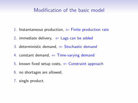
Modification of the basic model
1. Instantaneous production, ⇐ Finite production rate
2. immediate delivery, ⇐ Lags can be added
3. deterministic demand, ⇐ Stochastic demand
4. constant demand, ⇐ Time-varying demand
5. known fixed setup costs, ⇐ Constraint approach
6. no shortages are allowed,
⇐ Shortages are allowed
7. single product.
⇐ Multiple products
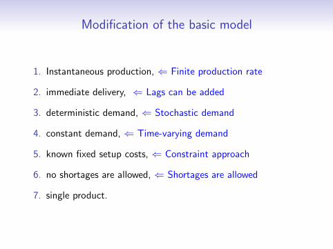
Modification of the basic model
1. Instantaneous production, ⇐ Finite production rate
2. immediate delivery, ⇐ Lags can be added
3. deterministic demand, ⇐ Stochastic demand
4. constant demand, ⇐ Time-varying demand
5. known fixed setup costs, ⇐ Constraint approach
6. no shortages are allowed, ⇐ Shortages are allowed
7. single product.
⇐ Multiple products
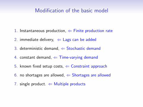
Modification of the basic model
1. Instantaneous production, ⇐ Finite production rate
2. immediate delivery, ⇐ Lags can be added
3. deterministic demand, ⇐ Stochastic demand
4. constant demand, ⇐ Time-varying demand
5. known fixed setup costs, ⇐ Constraint approach
6. no shortages are allowed, ⇐ Shortages are allowed
7. single product. ⇐ Multiple products
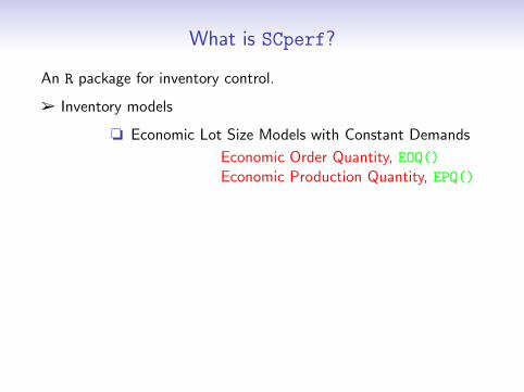
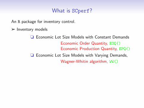
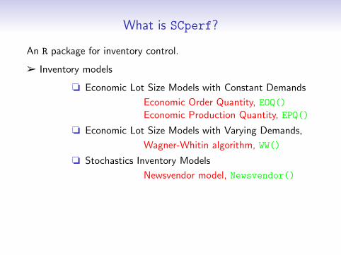
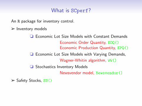
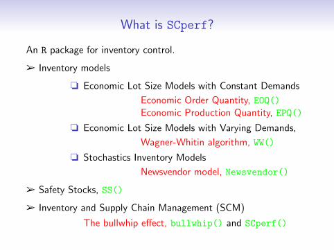
What is SCperf?
An R package for inventory control.
â Inventory models
o Economic Lot Size Models with Constant Demands
Economic Order Quantity, EOQ()Economic Production Quantity, EPQ()
o Economic Lot Size Models with Varying Demands,
Wagner-Whitin algorithm, WW()
o Stochastics Inventory Models
Newsvendor model, Newsvendor()
â Safety Stocks, SS()
â Inventory and Supply Chain Management (SCM)
The bullwhip effect, bullwhip() and SCperf()
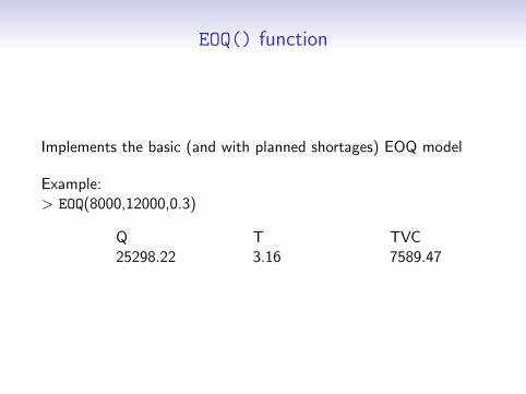
EOQ() function
Implements the basic (and with planned shortages) EOQ model
Example:> EOQ(8000,12000,0.3)
Q25298.22
T3.16
TVC7589.47
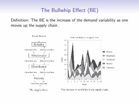
The Bullwhip Effect (BE)
Definition: The BE is the increase of the demand variability as onemoves up the supply chain.

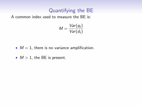
Quantifying the BEA common index used to measure the BE is:
M =Var(qt)
Var(dt)
� M = 1, there is no variance amplification.
� M > 1, the BE is present.
� M < 1, smoothing scenario.
Zhang 2004:
M = 1 +2∑L
i=0
∑Lj=i+1 ψiψj∑∞
j=0 ψ2j

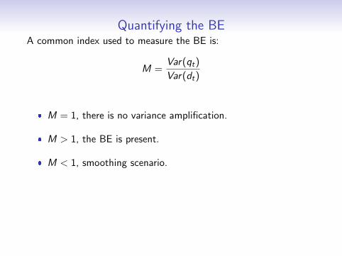
Quantifying the BEA common index used to measure the BE is:
M =Var(qt)
Var(dt)
� M = 1, there is no variance amplification.
� M > 1, the BE is present.
� M < 1, smoothing scenario.
Zhang 2004:
M = 1 +2∑L
i=0
∑Lj=i+1 ψiψj∑∞
j=0 ψ2j
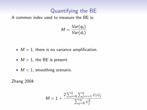
Quantifying the BEA common index used to measure the BE is:
M =Var(qt)
Var(dt)
� M = 1, there is no variance amplification.
� M > 1, the BE is present.
� M < 1, smoothing scenario.
Zhang 2004:
M = 1 +2∑L
i=0
∑Lj=i+1 ψiψj∑∞
j=0 ψ2j
Quantifying the BEA common index used to measure the BE is:
M =Var(qt)
Var(dt)
� M = 1, there is no variance amplification.
� M > 1, the BE is present.
� M < 1, smoothing scenario.
Zhang 2004:
M = 1 +2∑L
i=0
∑Lj=i+1 ψiψj∑∞
j=0 ψ2j
Quantifying the BEA common index used to measure the BE is:
M =Var(qt)
Var(dt)
� M = 1, there is no variance amplification.
� M > 1, the BE is present.
� M < 1, smoothing scenario.
Zhang 2004:
M = 1 +2∑L
i=0
∑Lj=i+1 ψiψj∑∞
j=0 ψ2j
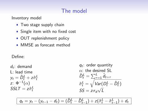
The modelInventory model
� Two stage supply chain
� Single item with no fixed cost
� OUT replenishment policy
� MMSE as forecast method
Define:
dt : demandL: lead timeyt = D̂L
t + z σ̂Ltz : Φ−1(α)SSLT = z σ̂Lt
qt : order quantityα: the desired SLD̂Lt =
∑Lτ=1 d̂t+τ
σ̂Lt =√
Var(DLt − D̂L
t )
SS = zσd√L
qt = yt − (yt−1 − dt) = (D̂Lt − D̂L
t−1) + z(σ̂Lt − σ̂Lt−1) + dt
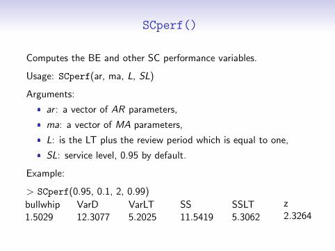
SCperf()
Computes the BE and other SC performance variables.
Usage: SCperf(ar, ma, L, SL)
Arguments:
� ar : a vector of AR parameters,
� ma: a vector of MA parameters,
� L: is the LT plus the review period which is equal to one,
� SL: service level, 0.95 by default.
Example:
> SCperf(0.95, 0.1, 2, 0.99)
bullwhip1.5029
VarD12.3077
VarLT5.2025
SS11.5419
SSLT5.3062
z2.3264
Why did we develop SCperf?
� Educational purposes:to offer to useRs, teachers, researchers and managers a free,open-source, package for inventory control
� Managerial purposes:might be used as an alternative (or complement) to otherSCM commercial packages.
� The long-term goal of SCperf is to implement the lastresearch in inventory control theory as well as all thestate-of-the-art capabilities that are currently available incommercial packages.
