master thesis tamas major
TRANSCRIPT

Master Thesis
Automotive Powertrain Modeling with the Focus on the Clutch Element
Major Tamas
──────────
Supervisior: Dipl. -Ing. Dr. techn. Univ. Doz. Daniel Watzenig
Institute of Electrical Measurement and Measurement Signal Processing
Graz University of Technology
Co-Supervisior: Dipl. –Ing. Dr. techn. Josef Zehetner
Kompetenzzentrum - Virtual Vehicle Area E
Graz, December 2011
Page 3
Abstract
The main goal of this master thesis was to develop a simplified but realistic clutch model in MATLAB/Simulink which is capable of operating in real-time. In order to build-up an appropriate test environment it is essential to model other powertrain elements such as engine, transmission, drive shaft and acting driving resistance. There were two important requirements during the development of the model:
• Modularity • Real-time capability
The developed model is capable for the integration in control design processes or the simulation of complex hybrid powertrain architectures. At the beginning, the theoretical part gives an overview about a simplified powertrain structure, furthermore describes the importance of a clutch itself and summarizes the existing gear shifting- and hybrid concepts. Then in the implementation part, the existing clutch modeling concepts have been investigated to point out the differences and similarities. Thus, not only so-called the classic, but the sliding mode model was built up to simulate a drive away process of the vehicle. After validating the simulation model using synthetic data, another key point was to validate the investigated models with measurement data. Finally, some future research directions have been pointed out and discussed for further development of the concepts.

Page 4
Kurzfassung
Das Hauptziel dieser Diplomarbeit war es, ein vereinfachtes, aber realistisches Kupplungsmodell in MATLAB-Simulink zu entwickeln. Um realistische Simulationsergebnisse zu erhalten, müssen sämtliche Antriebstrangelemente wie Motor, Getriebe, Welle und Fahrwiderstände modelliert werden.
Während der Entwicklung des Modells stellten Modularität und Echtzeitfähigkeit die wichtigsten Anforderungen dar.
Am Anfang des theoretischen Teils ist ein Modell der Antriebstrangstruktur abgebildet. In weiterer Folge wird die Funktion sämtlicher Bauteile beschrieben, wobei große Aufmerksamkeit auf die Kupplung gelegt wird. Diese spielt bei der Antriebsstrangsimulierung eine zentrale Rolle.
Anschließend erfolgt die Ausarbeitung zweier verschiedener Modellierungskonzepte. Nachdem bei der Simulierung eines einfachen Anfahrvorganges realistische Ergebnisse entstehen, kommt es zur weiteren Entwicklung des Modells mittels gemessener Validierungsdaten. Daraufhin werden die Vor- und Nachteile der jeweiligen Modellierungskonzepte gegenübergestellt, wobei beide Lösungsvarianten ähnliche Ergebnisse liefern sowie Stärken und Schwächen besitzen. Schließlich werden einige Vorschläge für die weitere Entwicklung des Modells erwähnt.
Dieses Modell kann schließlich in Control Design-Prozessen oder bei der Modellierung komplizierter Hybrid- Antriebstrangstrukturen verwendet werden. Diese Diplomarbeit wird denjenigen empfohlen, die Kupplungsmodellierungskonzepte näher kennenlernen möchten.

Page 5
Acknowledgements
At the end of my master education, I wish to thank all the people that supported me in this academic experience. Special thanks go to my supervisor Daniel Watzenig for its availability and helpfulness. Similar thanks goes to my co-supervisor Josef Zehetner for its support and friendship in the difficult moments. A particular thanks go to my colleges in Virtual Vehicle: Petr Micek and Bernhard Knauder. I will never forget the assistance of my college Walter Rosinger in helping me with his great advices. Prof. Sándor Tóth from the Technical University of Budapest gave also many advices to fulfill my master thesis.
I owe great thanks for my mother and father, for making this education possible and their trust.
Finally I would like to thank to my girlfriend Nóra, for encouraging me in the difficult moments.

Page 6
Contents
Abstract ..................................................................................................................... 3
Kurzfassung .............................................................................................................. 4
Acknowledgements .................................................................................................. 5
Contents .................................................................................................................... 6
List of symbols .......................................................................................................... 8
1 Introduction .................................................................................................. 10
1.1 Motivation ..................................................................................... 10
1.2 Problem statement ...................................................................... 11 1.3 State-of-the-Art ............................................................................. 13
1.4 Added Value ................................................................................. 16
1.5 Structure of the thesis................................................................. 16
2 Theory ........................................................................................................... 17
2.1Introduction ................................................................................... 17
2.2 Modeling ....................................................................................... 17
2.3 Powertrain ..................................................................................... 19
2.3.1 Engine ........................................................................... 20
2.3.2 Clutch ............................................................................ 20
2.3.3 Gearbox ........................................................................ 22
2.3.4 Drive Shaft .................................................................... 23 2.3.5 Differential .................................................................... 24
2.3.6 Vehicle Chassis and Wheels (Resistances) ............... 24

Page 7
3 Implementation ............................................................................................. 27 3.1Introduction ................................................................................... 27
3.2 Vehicle Simulation Model ............................................................ 27
3.2.1 Engine ........................................................................... 29
3.2.2 Gearbox + Drive Shaft + Differential ........................... 33
3.2.2.1 Transmission ........................................... 33
3.2.2.2 Drive Shaft ................................................ 35
3.2.2.3 Differential ................................................ 36
3.2.3 Vehicle Chassis and Wheels (Resistances) ............... 37
3.2.4 Clutch ............................................................................ 40
4 Simulation Results ....................................................................................... 49
4.1Introduction ................................................................................... 49 4.2 Drive Away Simulations............................................................... 50
4.2.1 Classic Model ............................................................... 50
4.2.2 Sliding Mode Model ..................................................... 53
4.3 Validation ...................................................................................... 56
5 Conclusion and Future Work ............................................................................ 62
6 References ......................................................................................................... 63

Page 8
List of Symbols
eJ engine inertia
eω angular velocity of the engine
eT engine torque
cT torque through the clutch
eb engine damping factor
c,eω common angular velocity when the clutch locked
trT transmission torque
shaftT shaft torque
i actual gear ratio
shaftω angular velocity of the shaft
sk stiffness of the shaft
dk damping factor of the shaft
diffω angular velocity of the differential
diffdi gear ratio of the differential
diffT torque of the differential
vehicleω angular velocity of the wheels
xF longitudinal force acting on the wheels
r,xF drag force of the vehicle
aF air resistance force
σ air density
A frontal surface area
fc air friction coefficient

Page 9
v vehicle speed
gF gradient resistance force
m mass of the vehicle
g acceleration due to gravity
α slope of the road
rF rolling resistance force
4r1,r0,r f;f;f rolling resistance coefficients
cJ clutch inertia
cω angular velocity of the clutch
NF normal actuation force on the clutch plate
µ friction coefficient of the clutch surface
aR active friction radius of the clutch
0r outer radii of the clutch plate
ir inner radii of the clutch plate
smaxfT torque capacity of the clutch
relω relative velocity between the engine and the clutch
meanT mean value of the engine torque

Page 10
1. Introduction
1.1 Motivation
In the automotive industry where time factor is crucial, in order to reduce time and costs for development, computer aided techniques have already been introduced. During the modeling of a powertrain structure, there are some non-linear components such as clutches or tires. The clutches are of major importance among all. The fact that the system degrees of freedom depends on the clutch’s current state, makes the modeling much more complicated. Many advanced controller schemes contain a plant model as part of the controller design. Therefore, the automotive industry is strongly motivated to develop such models. Real-time capability also plays an important role in the development of embedded applications. For the cost-effectiveness of producing such systems, modularity is indispensable. Modular simulation models can be reused for modeling other, more complex structures such as hybrid drivelines or double clutch transmission.

Page 11
1.2 Problem statement
The main goal of the Master Thesis is to implement and test a basic library of simplified, but yet sufficiently accurate simulation models of typical driveline components. These elements are: the engine, clutch, transmission, drive shaft and vehicle chassis. Among these elements the greatest emphasis is put on the clutch. Depending on the torque demand, there are two basic concepts of friction clutches available. These concepts are dry- and wet friction clutches. Wet multi disc clutches are used for applications with higher torque capacity where there is more energy to handle and more heat to dissipate [1]. During the simulation a dry friction clutch has to be realized with manual transmission. From the model structure point of view, all models should reflect the relevant physical phenomena. One of the main requirements is the real-time capability and modularity of the implemented models. To simplify practical application of developed models, a realistic calibration procedure based on simple experiments and typical component specification should be proposed. An automotive powertrain is shown in Figure 1. Each component has to be modeled as a separate element in order to create a modular simulation environment.
The main components to be modeled are:
• engine model, important signals to be calculated: o torque o angular velocity at the output shaft
• clutch model, important signals to be calculated:
o transmitted torque o clutch slip o angular velocity
• gearbox model, important signals to be calculated:
o transmitted torque o gearbox output inertia converted to gearbox input o angular velocity
• powertrain damping elements, important signals to be calculated:
o transmitted torque

Page 12
o angular speed of input and output shafts (flanges) o relative angular displacement of flanges
• vehicle resistance model, important signals to be calculated:
o vehicle speed and acceleration
Figure 1. An automotive powertrain structure with the main elements [2].

Page 13
1.3 State-of-the-Art
The main components of an IC – engine - based powertrain systems are the engine and the gearbox. Gearboxes are transform the power provided by the engine at a certain speed and torque level to a different speed and torque level. Clutches are also a part of such systems. These elements are necessary to kinematically decouple, for a short period of time, the engine from the vehicle [3]. From the modeling point of view the engine can be seen as a source that generates torque at the output shaft and the clutch transmits this torque to the gearbox. Figure 2 depicts a simplified modeling structure of a dry clutch system.
Figure 2. Simplified modeling structure of a dry clutch system. This element is located between the engine (left) and the gearbox (right) [5].
During the transmission where strong non-linearities (i.e. coulomb friction) affect the system dynamics, it can happen that the system behaves as a lower order system. There are two operating modes of the clutch:
• Slipping – the two plates of the clutch have different angular velocities
• Sticking – the two plates rotate together with the same angular velocity

Page 14
When the clutch is slipping, the two inertias are moving with the different angular velocities independently under the action of the torques from the engine output and the gearbox input, and only the coulomb friction is exchanged between them. Otherwise, when the clutch is locked, the two inertias rotate together with the same angular velocity. The simulation of this type of systems is not easy due to the fact that the model changes its order [4]. As the system loses a degree of freedom, the transmitted torque goes through a step discontinuity. The magnitude of the torque through the clutch drops from the maximum value supported by the friction capacity to a value that is necessary to keep the two halves of the clutch spinning at the same speed [5]. A common method to simulate systems mentioned above is the modeling with multi-subsystems. The block scheme used in this case is shown in Figure 3: in every moment the logic chooses which model has to be used.
Figure 3. Multi-subsystem modeling concept [16]

Page 15
As mentioned above the clutch has two states so in this example two different sub-models are needed. With this simulation, the following problems arise [4]:
• The number of the different models increases exponentially with the number of the masses [6].
• When the system switches from one model to another, the updating of the initial conditions of the new model is required.
• Inputs and outputs of the simulator have to be properly connected to the new model.
• At every moment of the simulation time, the logic has to decide which one, among all possible models, is the correct model to be used at that time.
For all these reasons, this simulation model is generally too complex to be used when the number of masses is greater than 3.

Page 16
1.4 Added value
An alternative realization to the clutch simulation is a sliding mode model. As discussed above the simulation with multi-subsystems causes many problems. In sliding mode the same mathematical equations have been used during the simulation, so it is unnecessary to change between different states. The consequence is that there is no need for a logic block. For a comparison and evaluation of the two methods, both models have been created within this work, bearing in mind with the main requirements such as modularity and real time capability. Considering that the only difference between the two modeling structures is in the clutch block (and every other element are the same with the same parameters) an appropriate comparison is possible. In Chapter 3.3 a drive away process of the vehicle will be simulated in both modeling environment and compared as well. After the drive away simulation gave a realistic behavior in Chapter 3.4 the validation simulations in both cases are represented.
1.5 Structure of the thesis
The Master Thesis is divided into three main chapters. Chapter 2 summarizes all the relevant information about powertrain elements and modeling methods. This information is essential to understand the modeling concept, used in the third Chapter where the MATLAB/Simulink realizations of the powertrain elements are presented. Both modeling constructions will be compared in this Chapter.
Chapter 4 discusses all the drive away simulations. Also the validation simulation is addressed in the final chapter.

Page 17
2. Theory
2.1 Introduction
This chapter briefly discusses the two main modeling concepts for technical applications. The expression powertrain and the expectations are also introduced as well. After that there is an overview of various powertrain elements such as engine, clutch, gearbox, shaft, differential and wheels with the purpose of each element. In the section Gearbox the most commonly used gear shifting concepts have been collected.
2.2 Modeling
The temporal behavior of technical systems can be described with uniform methods from the system theory. The main goal of these methods is to create an appropriate mathematical expression that correctly models the static and dynamic behavior of the technical process. The determination of these mathematical models based either on theoretical or an experimental way. In the theoretical modeling, the mathematical expression is created on the basis of natural laws [21]. This method always begins with simplifying assumptions about the process to facilitate the calculation.
On the other hand the experimental modeling, also called Identification, determine the mathematical model of a process from measurement values as follows. First the input and output signals will be measured and evaluated with the appropriate identification method. As a result a mathematical relationship between the input and output is established [21]. Figure 4 shows various methods for modeling of dynamic processes based on these two main methods.
During the Master Thesis an automotive clutch system has to be modeled with other powertrain components. The dynamic behavior of a clutch can be described with different motion equations in appropriate states (stick, slip).

Page 18
In the system theory these types of systems called Variable Structure System (VSS). Paper [22] introduces some advantageous properties of a VSS and also describes a motion type of trajectories, so called the sliding mode motion. This motion will be described in the Implementation part in more detail.
Figure 4. Various methods of modeling dynamic processes [21]

Page 19
2.3 Powertrain
In the automotive sector, the powertrain is a general expression to a group of elements that propels the car. The drivetrain is the complete powertrain except the engine. During the development of an automotive powertrain system there are several requirements which have to be fulfilled. As an example an effective utilization of a power provided by the engine is crucial. Reducing the fuel consumption is also an essential requirement in modern automotive solutions. The concept of a hybrid powertrain is a challenging improvement in the current powertrain architectures. In accordance with the technical requirements many different powertrain configurations exist, such as front wheel drive, all wheel drive and hybrid powertrain; however there are certain elements which can be found in almost every structure. Some examples of these elements: engine, clutch, gearbox, driveshaft, differential and the wheels. For simulation purposes, this group has to be extended with a simplified vehicle resistance model. Figure 5 illustrates a powertrain configuration with the main elements mentioned above.
Figure 5. A schematic picture of an automotive powertrain configuration [7].

Page 20
2.3.1 Engine
In every powertrain structure, the main purpose of the engine is to ensure the torque that guarantees the movement of the vehicle in all circumstances. This torque appears at the output side of the engine, also called flywheel. During the operation not only torque has been created. Heat and emission is also delivered by the engine. The driver can control the operation of the engine via the throttle pedal position. From the modeling point of view, the engine is a block where the input is the throttle pedal position actuated by the driver and the output is the delivered torque at a certain angular velocity.
2.3.2 Clutch
One of the main purposes of a clutch system in cars, trucks and other vehicles is to gradually engage the engine to the drivetrain while avoiding unpleasant shocks, jerks and excessive drivetrain wear [8]. This engagement is necessary to make gear shifting possible to the driver. The method of gear shifting will be discussed in the next subsection, so called Gearbox. Furthermore this element is a starting element which is essential in those powertrain structures where the power source is an internal combusting engine. Basically, the clutch needs three parts to transmit torque. These are the flywheel mentioned above, a friction disc also called the clutch disc and a pressure plate. The clutch disc is located between the flywheel of the engine and the pressure plate. The pressure plate is connected to the gearbox and the remaining part of the powertrain. Figure 6 displays the main clutch elements from the flywheel to the release fork. These elements are [10]:
• a diaphragm-spring clutch cover bolted to the flywheel, • a clutch disc with two friction facings that is capable of moving
axially on the gearbox input shaft, • a torsional vibration damper integrated into the clutch disc, and • a releaser which transfers clutch release travel from the non-
rotating actuating elements to the clutch cover by means of a ball bearing.
Page 21
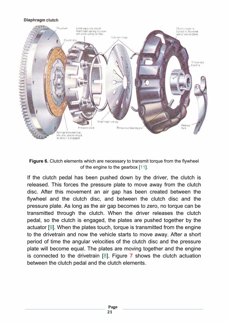
Figure 6. Clutch elements which are necessary to transmit torque from the flywheel of the engine to the gearbox [11].
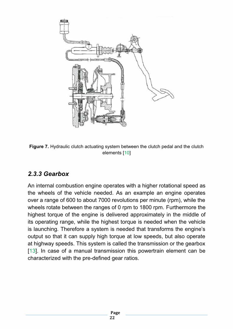
If the clutch pedal has been pushed down by the driver, the clutch is released. This forces the pressure plate to move away from the clutch disc. After this movement an air gap has been created between the flywheel and the clutch disc, and between the clutch disc and the pressure plate. As long as the air gap becomes to zero, no torque can be transmitted through the clutch. When the driver releases the clutch pedal, so the clutch is engaged, the plates are pushed together by the actuator [9]. When the plates touch, torque is transmitted from the engine to the drivetrain and now the vehicle starts to move away. After a short period of time the angular velocities of the clutch disc and the pressure plate will become equal. The plates are moving together and the engine is connected to the drivetrain [8]. Figure 7 shows the clutch actuation between the clutch pedal and the clutch elements.
Page 22
Figure 7. Hydraulic clutch actuating system between the clutch pedal and the clutch elements [10]
2.3.3 Gearbox
An internal combustion engine operates with a higher rotational speed as the wheels of the vehicle needed. As an example an engine operates over a range of 600 to about 7000 revolutions per minute (rpm), while the wheels rotate between the ranges of 0 rpm to 1800 rpm. Furthermore the highest torque of the engine is delivered approximately in the middle of its operating range, while the highest torque is needed when the vehicle is launching. Therefore a system is needed that transforms the engine’s output so that it can supply high torque at low speeds, but also operate at highway speeds. This system is called the transmission or the gearbox [13]. In case of a manual transmission this powertrain element can be characterized with the pre-defined gear ratios.

Page 23
The input shaft of the gearbox is connected to the friction disc of the clutch. Several gear shifting concepts have been developed by the automotive industry. Figure 8 gives a short overview about the most commonly used gear shifting concepts. In the framework of the Master Thesis the manual shifting concept will be modeled.
Figure 8. A schematic classification of the existing gear shifting concepts [13].
2.3.4 Drive Shaft
The drive shaft is connected to the output of the gearbox. This is a mechanical element, developed for transmitting rotation and torque. An automobile use a longitudinal shaft to deliver torque from the engine through the differential to the wheels. This element is characterized by stiffness and damping. Figure 9 depicts a drive shaft.

Page 24
Figure 9. Drive shaft1 with universal joint at each end and a spline in the centre [14].
2.3.5 Differential
Similarly to the drive shaft, the differential is transmitting rotation and torque. However, this element is proposed to transmit the torque and rotation from the input, to two perpendicular axes where the wheels are mounted. The drive shaft can be characterized with a fix gear ratio called the final drive ratio.
2.3.6 Vehicle Resistance
An automotive transmission is located between the engine and the drive wheels. The transmission fits the power supply of the engine to the requirements of the drive wheels by converting the torque and the speed. The power requirement at the drive wheels is calculated by the vehicle resistances [13]. The vehicle resistance consists the following main components listed below [13]:
• Wheel Resistance • Air Resistance • Gradient Resistance
1 Wikipedia (22/10/2011). Available: http://en.wikipedia.org/wiki/Drive_shaft. Last accessed: 24/10/2011

Page 25
Wheel Resistance
Wheel resistance means the resisting forces acting on the driving wheels. It contains the following elements [13]:
• rolling resistance • road surface resistance and the • slip resistance
Since driving simulations mainly calculate on a dry surface, rolling resistance is the dominant wheel resistance [13]. The mathematical equations will be summarized in the implementation part.
Air Resistance
Every moving vehicle has an air resistance which calculated from the following components [13]:
• induced drag • surface resistance • internal resistance
The air resistance is a quadratic function of the flow rate. The flow rate is calculated from the sum of the vehicle speed and the wind speed component in the direction of the vehicle longitudinal axis. Driving simulations assume mainly calm, so the flow rate is equals to the vehicle speed [13]. As well as the wheel resistance, the main equation of the air resistance will be explained in the implementation part.
Gradient Resistance
Considering the fact the in a real atmosphere of the vehicle not only flat surfaces occur, it is necessary to introduce a slope of the traveling surface. The gradient resistance relates to the slope descending force and is calculated from the weight acting at the centre of gravity [13]. The road gradient q is defined as the quotient of the vertical and horizontal projections of the roadway. Figure 10 shows the forces acting on the vehicle travelling uphill [13].

Page 26
Figure 10. Forces acting on the vehicle traveling uphill [13]
All the relevant equations of the vehicle resistance model will be discussed in the implementation part.

Page 27
3. Implementation
3.1 Introduction
The theoretical background of this model was discussed in the theory part of this thesis. The elements of the powertrain were treated as separate blocks. In the following section, the MATLAB/Simulink realization of the main elements is presented of each modeling structure, taking the physical properties of each into account. The applied motion equations together with the parameters are also presented in this part of the thesis.
The benefits and also the disadvantages of this simulation environment will be discussed as well.
3.2 Vehicle Simulation Model
The powertrain model was developed in MATLAB/Simulink environment. MATLAB2 is a software package, developed for solving numerical mathematical problems especially with vectors and matrixes. The program provides a variety of additional packages (Toolboxes) to solve numerous technical problems in different applications. Some examples of such toolboxes are: Stateflow, Control System or Signal Processing. For modeling purposes MathWorks developed a toolbox, so called Simulink. This is a graphical interface to model different physical problems with signal-flow graphs. A signal-flow graph has a one-to-one relationship with the motion equations of a physical system. It is a common method to represent the signal flows in any technical systems with relations of cause and effect [23]. Taking into account that the physical laws are available in the modeling and furthermore Simulink provides a fixed-step solver, MATLAB/Simulink is an optimal environment to set up a simulation model for automotive applications. Simulink provides two major solver types:
2 www.mathworks.com

Page 28
• Fixed-step • Variable-step
Both fixed-step and variable-step solvers calculate the next simulation time as a sum of the current simulation time and a quantity so called the step size [12]. With a fixed-step solver the step size remains constant throughout the simulation while the variable-step solver can vary the step size depending on the dynamics of the model [12]. Using a fixed-step solver has many advantages in the future use among various automotive applications. Fixed-step solver allows an accurate estimation of the computing time which is very important for a future hardware application [14]. Additionally with a fixed-step solver it is possible to compare the simulation results with measurement values [14]. One of the main objectives of the thesis was to create a model that works in real-time environment.
With a fixed-step solver it is possible to generate a code from the model and then run the code on a real-time computer system [14]. Modularity was also an important requirement of the thesis. In terms of modularity the created model has some limitations. Between the individual blocks the power exchanges in form of torque and angular velocity. The consequence of this modeling approach is, in case of a change of an input or output, the whole structure has to be modified accordingly. Performace-based modeling would be an optimal solution for this problem. Looking the top level of the modeling structures, it is visible, that the only significant difference is in the clutch block. In order to facilitate comparison, both of the constructions will be presented in every subsection at the same time. Figure 11 shows the top level structure of a classical solution.

Page 29
Figure 11. Top level structure of an automotive powertrain system in MATLAB - Simulink
This model has two initial parameters. These are the initial vehicle speed and the slope of the road surface. During the simulation both of the initial values are set to zero. Furthermore, the model consists of three external input variables. These are the throttle position, the clutch pedal position and the actual gear ratio. These values are essential to start a simulation.
3.2.1 Engine
In this work, the internal combusting engine (ICE) is modeled as a torque source that has a variable output due to the engine speed. In both modeling constructions a lookup table containing the ICE’s torque – speed characteristics [15], also called torquemap, is built. The calculated speed value is used as the input, thus the output is the torque of the engine in that speed. Figure 12 shows the torquemap of the ICE. It is apparent that, in case of the throttle pedal is not operated or actuated; the torquemap assigns a negative torque value to every engine speed. In such cases, the engine torque should be zero, as will be seen in the validation, so it was necessary to extend both of the engine blocks with an idle speed control unit.
Tdif f wv ehicle
VEHICLE RESISTANCE MODEL
Gear
wc
Tshaf t
ws haf t
Ttr
TRANSMISSION
wshaf t
wdif f
Tshaf t
SHAFT
gears_soll
gaspedal_soll cl_pos_soll
T_en_out2
pedal_en_in
loc ked
w_en_out
T_en_out
ENGINE
Ts haf t
wv ehicle
Tdif f
wdif f
DIFFERENTIAL
clutch_pos
we
TE
Ttr
TC
locked
wc
CLUTCH

Page 30
Figure 12. Torque of the ICE as a function of a throttle position and the ICE speed
Idle speed is the rotational speed of the engine when is uncoupled from the drivetrain and the throttle pedal is not actuated [13]. This control unit compares the actual engine speed value with the idle speed. If the actual value goes below the idle speed the control unit overwrites the negative torque with the torque of zero. In addition a simplified damping factor ebwas also introduced in the engine block. The above mentioned elements have appeared in both versions of the engine block. The main difference between the two constructions is that the engine block of the classical solution contains a third input variable, so called the “locked” signal. This signal determines the actual state (Slip, Stick) of the clutch and will be calculated in the clutch block. In the classical realization the motion equations depending on the current state of the clutch, and the locked signal guarantees that during the simulation the correct equations will be used.
The following mathematical equations have been implemented in the engine block of the classical model [8]:

Page 31
Slipping:
eeceee bTTJ ω−−=ω⋅ & (3.1)
Sticking:
( ) eecec,ece bTTJJ ω−−=ω⋅+ & (3.2)
The notations are: ω is the angular velocity, J is the moment of inertia, b is a damping factor and T is the Torque. The subscripts used are: e is for the engine, c is for the clutch.
In sticking phase the angular velocity of the engine output- and the clutch output shaft are the same. In the classical model the common speed c,eωwill be computed in the engine block with the Equation (3.2). This common speed will be forwarded in Simulink through the clutch block into the transmission block. Figure 13 depicts the MATLAB/Simulink coupling plan of the engine block in the classical solution.
Figure 13. Simulink coupling plan of the ICE in the classical construction
To summarize the inputs of this block:
• throttle position with the range of [0…1], • locked signal with two values [0 and 1], and • torque through the clutch in Nm as a load, the range is determined
by the capacity of the clutch and in this simulation example this value is approximately [364].
we in [rad /s]
TE2
we1
be
30/pi engine _status
Idle Control Unit
we
Te
Te_controlled
we_locked
wc_unlocked
Engine _Torquemap
Engine _Speed
1s
xoEngine _Inertia
en _JE
100
Clutch _Inertia
cl_JG
locked3
TC2
Throttle1
[rad/s]
Inertia
TE in [Nm]

Page 32
The outputs are:
• speed of the engine in rad/s unit with the range of [0…660], and • the engine torque in Nm with the range of [0…181].
On the other hand the sliding mode model uses the same motion equation in every state of the clutch, thus there is no need a third logic signal to calculate the torque and the speed of the engine. This equation is the same as the Equation (3.1) in the classical solution. Figure 14 shows the Simulink coupling plan of the engine block in the sliding mode model.
Figure 14. Simulink coupling plan of the ICE in the sliding mode model
To summarize the inputs of this block:
• throttle position with the range of [0…1], and • clutch torque in Nm as a load, the range is determined by the
capacity of the clutch and in this simulation example this value is approximately [364].
The outputs are:
• speed of the engine in rad/s unit with the range of [0…660], and

Page 33
The following parameters have been used in both simulation environments [15]:
211.0Je = 2kgm
00746.0J c = 2kgm
09.0be = Nms
The torquemap was also taken from Dyna4 [15].
3.2.2 Transmission & Drive Shaft & Differential
As mentioned above, the main difference between the two constructions (Classic, SM) is in the clutch block. The motion equations of the following three elements (Transmission, Drive Shaft and Differential) are the same in both cases so it is adequate to describe one of them with the appropriate MATLAB/Simulink coupling plan.
3.2.2.1 Transmission
Transmissions are elements, in automotive vehicles, that transform the mechanical power provided by a power source (in this example the engine) at a certain speed and torque to a different speed and torque level [3]. Ignoring all loses that are caused by the transmission, the following motion equations were used during the simulation [3]:
iTT shaft
tr = (3.3)
ic
shaft
ω=ω (3.4)
where i means the actual pre-defined gear ratio in the transmission block, cω and shaftω are the angular velocities of the clutch and the shaft input respectively and finally trT and shaftT are the torques of the transmission and the drive shaft. The gear ratios were taken from [15]:

Page 34
[ ]68.0;88.0;15.1;6.1;45.2;3.4i =
In MATLAB/Simulink the gears were stored in a 1-D lookup table. Figure 15 depicts the coupling plan of the transmission in the classical solution. As been noted, the same equations were used in the sliding model as well.
Figure 15. Simulink coupling plan of the transmission in the classical solution
To summarize the inputs of this block:
• speed of the clutch cω in rad/s • torque from the drive shaft shaftT in Nm
The outputs are:
• speed of the input shaft of the drive shaft shaftω in rad/s • transmission torque trT at the input shaft of the transmission in Nm
3.2.2.2 Drive Shaft
As been noted above this element is used to transmit rotation and torque. The flexible shaft can be modeled as a rotational spring-damper system. This element is characterized with the following parameters:
500k s = rad/Nm
80k d =
2Ttr
1wshaft
1
.05s+1Transfer Fcn1
Lookup Table
3Tshaft
2wc
1Gear

Page 35
where sk and dk are the stiffness and damping coefficients respectively.
The following equation was used in the MATLAB implementation [8]:
( )( ) ( )diffshaftddiffshaftsshaft kkT ω−ω+ω−ω= ∫ (3.5)
Figure 16 depicts the coupling plan of the drive shaft.
Figure 16. MATLAB/Simulink coupling plan of the drive shaft
To summarize the inputs of this block:
• speed of the output shaft of the transmission shaftω in rad/s
• speed of the differential diffω in rad/s
The output is:
• torque of the drive shaft shaftT in Nm
3.2.2.3 Differential
This element divides the torque from the drive shaft to the wheels. It can be characterized with a parameter, so called the final drive ratio, which is equal [15]:
7.3didiff =
Figure 17 shows the Simulink realization of this element.
The following motion equations have been used to simulate the dynamic behavior of this element [8]:
diffshaftdiff diTT ⋅= (3.6)
diffvehiclediff di⋅ω=ω (3.7)
Stiffness
Damping
1Tshaft
1s
shaft_kp
shaft_ks
2wdiff
1wshaft

Page 36
To summarize the inputs of this block:
• the torque from the drive shaft shaftT in Nm • angular velocity of the wheels vehicleω in rad/s
The outputs are:
• the torque of the output shaft of the differential diffT in Nm • the angular velocity of the differential at the input shaft diffω in rad/s
Figure 17. Simulink coupling plan of the differential
3.2.3 Vehicle Chassis and Wheels (Resistances)
This component is crucial to simulate a powertrain construction. As noted in the theory part, this block is capable of modeling different resistance behaviors of the vehicle. To be precise, the air-, gradient- and the wheel resistances are considered. Chapter 2.3.6 described the physical background of these resistances. During the calculations the goal is to determine the vehicle speed. The following equation calculates the longitudinal force xF acting on the wheels [17]:
brakewheelrar,xx FFFFFF −−−−= (3.8)
2wdiff
1Tdiff
di_diff
2wvehicle
1Tshaft

Page 37
In the equilibrium Equation 3.8 it is apparent that the force appearing at the input r,xF has to be reduced with the appropriate resistances and as a result a longitudinal force is obtained. Figure 18 gives an overview about the main existing resistances of the automotive modeling. The following equations were used to determine the resistances [17]:
Air resistance force:
2fa vcA
21F ⋅⋅⋅σ⋅= (3.9)
Gradient resistance force:
( )α⋅⋅= singmFg (3.10)
Rolling resistance (Wheel):
( )4410r vfrvfrfrgmF ⋅+⋅+⋅⋅= (3.11)
Table 1 collects the relevant parameters in the vehicle resistance model [15]:
Name Letter Value Unit Wheel Radius r_dyn 0.32 m Frontal Surface Area A 2.00 m2 Air Density roh 1.2041 kg/m3 Air Friction Coefficient cf 0.65 Mass of the Vehicle m 1200.00 kg Rolling Resistance Coefficients fr0 0.01 fr1 0.2e-2 fr4 0.12e-2
Table 1. Parameters used in the vehicle resistance model
Based on Newton’s second law, the vehicle speed can be calculated from the longitudinal force xF as follows:
∫= dtFm1v xvehicle (3.12)

Page 38
Figure 18. The main vehicle resistances in the automotive modeling
Figure 19 depicts the Simulink coupling plan of the vehicle resistance model. During the simulation in both realization the same vehicle resistance model have been used.
Figure 19. MATLAB/Simulink coupling plan of the vehicle resistance model
Fx,r
Gradient Resistance
.
.
Wheel Resistance
.
.
Air Resistance
.
.
1wvehicle
0
roh
roh
mR
mR
mA
mA
3.6
m/s -> kph
9.81
g
cf
cf
alpha
alpha
sin
vehicle_status
ve_speed
> 0
|u|2
1/mA
Masse
1s
wv_unlocked
Goto
4
3.6
1/2
Gain
brake_measured
Divide1
Divide
ve_r_dyn
ve_r_dyn
brake_simulated
A
A
f(u)
1Tdiff
a_x v _x

Page 39
To summarize the input of this block:
• drag force r,xF in N
The output is:
• angular velocity of the vehicle vehicleω in rad/s
3.3 Clutch
In the Master Thesis the greatest emphasis was on this element. The mechanical structure of the clutch has been discussed in the theory part. As been noted in the introduction, the main goal of the thesis is to construct a simplified basic – but realistic – modeling structure to an automotive clutch system. In this subsection two commonly used modeling structures will be introduced. The first construction is the classical solution which is a simulation model with multi-subsystems (Figure 3). As been constructed in the engine block when the clutch is slipping the two inertias move independently and the angular velocity of the clutch will be calculated in the clutch block. Otherwise, when the clutch is sticking (locked), the two inertias rotate together and the common speed c,eω will be computed in the engine block. The clutch block consists of three sub-blocks in the classical solution. One for the logic to determine the state of the clutch (stick, slip), another calculates the torque through the clutch cT and the third block the angular velocity of the clutch cω . Figure 20 depicts the sub-level of the clutch block in the classical solution.

Page 40
Figure 20. MATLAB/Simulink sub-level structure of the clutch block in the classical solution
In slipping phase the following equations are valid to determine cT and cω[8]:
trccc TTJ −=ω⋅ & (3.13)
)(signRFT ceaNc ω−ω⋅⋅µ⋅= (3.14)
where cT is the torque from the transmission appeared as a load, NF is the normal actuation force on the clutch plate, µ is the friction coefficient of the clutch surface and the active radius [8] of the clutch plates are given by aR . Following equation is used to determine the active radius of the clutch [5]:
2i
2o
3i
3o
a rrrrR
−−
= (3.15)
where ir is the inner radii and or is the outer radii of the clutch disc.
A signum function ()sign is defined as follows [24]:
3wc
2locked
1TC
clutch_statusCLASSIC_TC.mat
To File
clutch_pos
TE
we
Ttr
wc
locked
TC
Tf maxs
TORQUE CLUTCH
TC
Ttr
we
locked
wc
SPEED CLUTCH
TC
Tf maxs
we
wc
locked
LOGIC
4Ttr
3TE
2we
1clutch_pos
f rom Engine
w f rom Engine
f rom Tr.
Page 41
−=
101
)x(sign ififif
0.>x,0x,0x
=<
(3.16)
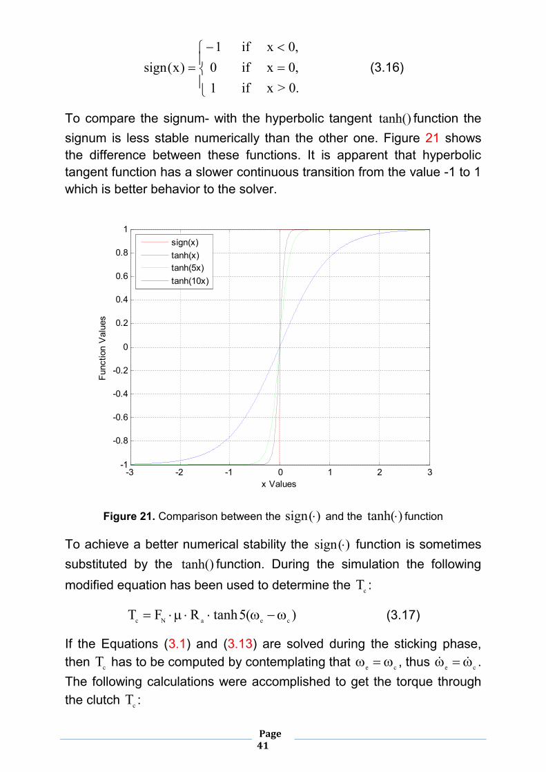
To compare the signum- with the hyperbolic tangent tanh() function the signum is less stable numerically than the other one. Figure 21 shows the difference between these functions. It is apparent that hyperbolic tangent function has a slower continuous transition from the value -1 to 1 which is better behavior to the solver.
Figure 21. Comparison between the )(sign ⋅ and the )tanh(⋅ function
To achieve a better numerical stability the )(sign ⋅ function is sometimes substituted by the tanh() function. During the simulation the following modified equation has been used to determine the cT :
)(5tanhRFT ceaNc ω−ω⋅⋅µ⋅= (3.17)
If the Equations (3.1) and (3.13) are solved during the sticking phase, then cT has to be computed by contemplating that ce ω=ω , thus ce ω=ω && . The following calculations were accomplished to get the torque through the clutch cT :
-3 -2 -1 0 1 2 3-1
-0.8
-0.6
-0.4
-0.2
0
0.2
0.4
0.6
0.8
1
x Values
Func
tion
Val
ues
sign(x)tanh(x)tanh(5x)tanh(10x)

Page 42
eeceee bTTJ ω⋅−−=ω⋅ &
trccc TTJ −=ω⋅ &
e
eecee J
bTT ω⋅−−=ω&
c
trcc J
TT −=ω&
Boundary conditions: ce ω=ω → ce ω=ω &&
c
trc
e
eece
JTT
JbTT −
=ω⋅−−
c
tr
c
c
e
ee
e
c
e
e
JT
JT
Jb
JT
JT
−=ω⋅
−−
e
c
c
c
c
tr
e
ee
e
e
JT
JT
JT
Jb
JT
+=+ω⋅
−
( ) ( )ce
cec
ce
etrceee
JJJJT
JJJTJbT
⋅+⋅
=⋅
⋅+⋅ω⋅−
( ) ( )cecetrceee JJTJTJbT +⋅=⋅+⋅ω⋅−
And the torque through the clutch in sticking phase is follows [8]:
( )c
ce
etrceee TJJ
JTJbT=
+⋅+⋅ω⋅−
(3.18)
Taking into account that the calculated torque cT could not exceed the maximum capacity of the clutch, it was necessary to build in a limitation, in form of a saturation block, into the clutch block. Figure 22 shows the Simulink coupling plan of the torque block inside of the clutch. It is also apparent that the “locked” signal switches between the Equation (3.17) and (3.18) in the appropriate cases.

Page 43
Figure 22. Simulink coupling plan to calculate the torque through the clutch in the classical solution
Inside the logic block the same logical terms are implemented as in the MATLAB/Simulink demo [5]. The Simulink coupling plan is shown in Figure 23.
Figure 23. Implemented logic to determine the state of the clutch (slip, stick) in the classical solution
2Tfmaxs
1TC
2*cl_R*cl_muk
TorqueConversion
tanh
up
u
lo
y
SaturationDynamic
cl_mus/cl_muk
Ratio of staticto kinetic
5
be
-1
Fn_max
cl_JG
en_JE
|u|
Abs
6locked
5wc
4Ttr
3we
2TE
1clutch_pos
Tf maxk
TC stick
TCmaxTCmax
1locked
locked
<
<
>
Mux
AND
100
cl_logic_l im i t
|u|
|u|
|u|
4wc
3we
2Tfmaxs
1TC
lock
unlock
slip [%]

Page 44
To summarize the inputs of this block:
• clutch pedal position pos_clutch with the range of [0…1] where 0 means not actuated and 1 indicates the fully actuated clutch pedal.
• speed of the engine eω in rad/s unit with the range of [0…660] • engine torque eT in Nm unit with the range of [0…181] • transmission torque trT in Nm where the range depends on the
actual transmission ratio, and
The outputs are:
• the torque through the clutch in Nm with the range of the capacity of the clutch, in this example is [-364…364]
• locked signal to determine the state of the clutch with two logic values [0 & 1], and
• speed of the clutch cω in rad/s unit
The second simulation model mainly based on the sliding mode theory [22]. In the control theory the sliding mode control (SMC) is a nonlinear control method that alters the dynamics of the nonlinear system by using a discontinuous signal that forces the system to “slide” along a cross section of the systems normal behavior [18]. Most of the automotive problems are highly nonlinear just like the stick-slip effect of a clutch system. The use of sliding mode control ideas in automotive control applications has also been published [19, 20]. It offers an alternative approximation simulation method to handle the clutch nonlinear behavior. The sliding mode simulation model is also an approximation model to handle the nonlinear behavior of the clutch. It can be obtained from the classical solution by replacing the Equation (3.18) with the Equation (3.14) [4]. When the relative velocities cerel ω−ω=ω are not zero, the dynamic behavior of the system remains the same as in the slipping phase in the classical solution with the Equation (3.17) [4].

Page 45
Otherwise, when the relative velocity relω becomes in the vicinity of zero, the corresponding friction torque cT starts switching at finite frequency between the two values smaxfT± , where smaxfT means the capacity (mechanical limitation) of the clutch, trying to keep to zero the relative velocity [4]. This effect is called chattering. To avoid this effect the sign function is substituted by a saturation function. As a result in this case, just one model is used to simulate the behavior of the whole system in every functional condition [4]. It is important to mention that this sliding mode simulation model is not identical with the commonly used Sliding Mode Control in nonlinear systems. However, paper [4] discusses that the dynamic behavior of the sliding mode simulation model is equivalent with the classical solution mentioned above. In the next chapter some simulation results will be prove this statement. Considering the fact that this method is just an approximation method, a certain degree of difference is expected. A logic unit is no longer necessary in the clutch block in the sliding mode construction. The MATLAB/Simulink coupling plan is shown in Figure 24.
Figure 24. Simulink coupling plan of the clutch block in sliding mode simulation
1TC
Saturation1
Product1
1/2
2*cl_R*cl_muk
Gain
3wg
2we
1clutch_position TCmaxk [Nm]TCmaxk [Nm]

Page 46
To summarize the inputs of this block:
• clutch pedal position position_clutch with the range of [0…1] where 0 means not actuated and 1 indicates the fully actuated clutch pedal.
• speed of the engine eω in rad/s unit with the range of [0…660] • speed of the transmission trω in rad/s unit where the range
depends on the actual transmission ratio
The output of this block is:
• torque through the clutch cT in Nm unit with the range of the capacity of the clutch, in this example is [-364…364]
Figure 25 compares the inputs and outputs of the clutch block in both cases.
Figure 25. Inputs and outputs of the clutch blocks in classical construction and sliding mode model
clutch_position
we
wtr
TC
Sliding Mode Clutch Model
clutch_pos
we
TE
Ttr
TC
locked
wc
Classic Clutch Model
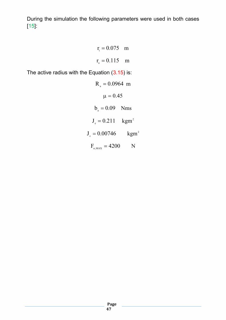
Page 47
During the simulation the following parameters were used in both cases [15]:
075.0ri = m
115.0ro = m
The active radius with the Equation (3.15) is:
0964.0R a = m
45.0=µ
09.0be = Nms
211.0Je = 2kgm
00746.0J c = 2kgm
4200F MAX,n = N

Page 48
4. Simulation Results
4.1 Introduction
In this chapter the simulation results will be introduced in both modeling environment. First a simplified driving situation, so called drive away, will be simulated with the same boundary conditions. After this simulation gave a physically correct result it comes to the validation. Validation is the process whereby the result of a simulation will be compared with the measured values on the real structure. During the development of a simulation model this phase is crucial for the evaluation of the constructed model. The measurement values, used in the validation, came from the software called Dyna4. This is a modular simulation software used in many applications in the automotive industry. It offers different products in different applications. Some examples of such products [15]:
Dyna4 Car Professional is the comprehensive real-time vehicle dynamics simulation software for virtual test and drives [15],
Dyna4 Advanced Powertrain is a simulation software for powertrain designs [15],
Dyna4 Driver Assistance is a simulation environment for the development and testing of advanced driver assistance systems [15].
Dyna4 Car Professional v1.0 was used to determine the validation values in the simulation.

Page 49
4.2 Drive Away Simulations
4.2.1 Classic Model
After the model structure and parameters are introduced, a drive away simulation will be presented. During this simulation, the vehicle started from standstill in first gear. The throttle pedal position is set to 18% for the entire simulation, which lasts 20 seconds. This test is designed to demonstrate the behavior of the vehicle in a simplified environment. Therefore, the gear does not change during the simulation. If the result gives unrealistic speeds, torques and angular velocities in this simplified situation, it becomes apparent that the current model still contains errors. Before the simulation results are presented a simplified calculation is introduced. Assuming that the angular velocity of the engine is limited to 6000 revolutions per minute (RPM), an approximate value of the vehicle speed can be determined. The simulated vehicle speed can be verified with this approximated value.
The maximal angular velocity of the engine in rad/s is:
62930
6000 ≈π
⋅s
rad
Considering that the first gear ratio is equal with 4.3 and the final drive ratio is 3.7 the maximal angular velocity on the wheels is:
5.397.33.4
629≈
∗ srad
The wheel radius is equal with 0.32m so the maximal speed of the vehicle in the first gear in km/h is:
5.456.332.05.39 ≈∗∗h
km
If the model exceeds this speed value that means some error is still inside the model.

Page 50
Figure 26 depicts the simulation results of the drive away simulation in the classical model. The first sub-plot shows the actuation force of the clutch and the second sub-plot shows the angular velocities of the engine and the clutch[5]. It is visible that the engine speed starts from an initial value and the clutch from the speed of zero. The velocity of the engine starts with an initial flare as the engine accelerates easily because it is separated from the rest of the powertrain[5]. At sec3t = , the clutch force starts to increase and as a consequence a friction is created between the two surfaces[5]. This appears as a load to the engine thus the engine speed starts to decrease while the clutch disc speed increases. At about sec777.3t = , the velocities are became equal and continue to increase until the engine reaches the maximum speed[5]. This maximal value has been reached at sec15t = as depicted in the second sub-plot of the Figure 26. It is also important to mention that in the third sub-plot the vehicle speed follows the clutch speed with the maximal value of 38.87 km/h which is a realistic value (see the calculations above). The locked signal changes (in the fourth sub-plot) from zero the one at 777.3t = sec as expected.
An important behavior can be observed on the fifth sub-plot of the Figure 26 where the relevant torques are presented. It is visible that the clutch torque exceeds the engine torque. This is normal and the following explanation proves this statement.
Figure 27 presents the angular velocities and the torques in another subplot. The first sub-plot shows that the velocity of the engine at the time 75.3t = sec equals with 239 s/rad and later at 8.3t = sec has a value of 203 s/rad . The appropriate torques of the engine at these time values are 75and 69 Nm respectively. The mean value of the engine torque and the angular acceleration in this time period are calculated as follows:
Nm722
6975Tmean =−
=
2srad720
75.38.3203239
=−−
=ω&

Page 51
Figure 26. Drive away simulation results in the classical solution
Assumed the engine inertia is 211.0 2kgm :
Nm152211.0720 ≈⋅ This torque is generated in the breaking period of the engine. To sum up, at the input shaft of the transmission appears the mean value of the engine torque (72 Nm) with the additional braking torque (152Nm). As a result Nm22415272 =+
0 2 4 6 8 10 12 14 16 18 200
100020003000
Time [s]
Forc
e [N
]Drive Away Simulation Classic Model
Clutch Actuation Force
0 2 4 6 8 10 12 14 16 18 20
0200400600
Time [s]
Vel
ocity
[rad
/s]
Engine SpeedClutch Speed
0 2 4 6 8 10 12 14 16 18 200
50
X: 17.54Y: 38.87
Time [s]
Spe
ed [k
m/h
]
Vehicle Speed in [km/h]Vehicle Acceleration in [m/s²]
0 2 4 6 8 10 12 14 16 18 20-1
0
1
2
Time [s]
Lock
ed S
igna
l
Locked Signal
0 2 4 6 8 10 12 14 16 18 200
100
200
300
Time [s]
Torq
ue [N
m]
Engine TorqueClutch TorqueTransmission Torque

Page 52
This increase of the torque (in compare with the engine torque) is available until the engine is slowed down by the clutch and hence its kinetic energy is available. When the braking period is finished, the torque through the clutch decreases significantly (as plotted in the second sub-plot of the Figure 27). Based on all these explanations, it is proved that the simulation results of the classical solution are correct and realistic.
Figure 27. Torques and angular velocities of the engine and clutch in the classical solution

Page 53
4.2.2 Sliding Mode Modeling Simulation
To achieve a suitable comparison, it is essential to match the simulation environments in the models. Therefore, both the inputs and the initial conditions are the same as in the classical model. Thus the throttle pedal position is set to 18%, the gear does not change during the simulation and the clutch actuation force is also the same. Figure 28 shows the results of the drive away simulation with the sliding mode model.
Figure 28. Drive away simulation results in the sliding mode solution
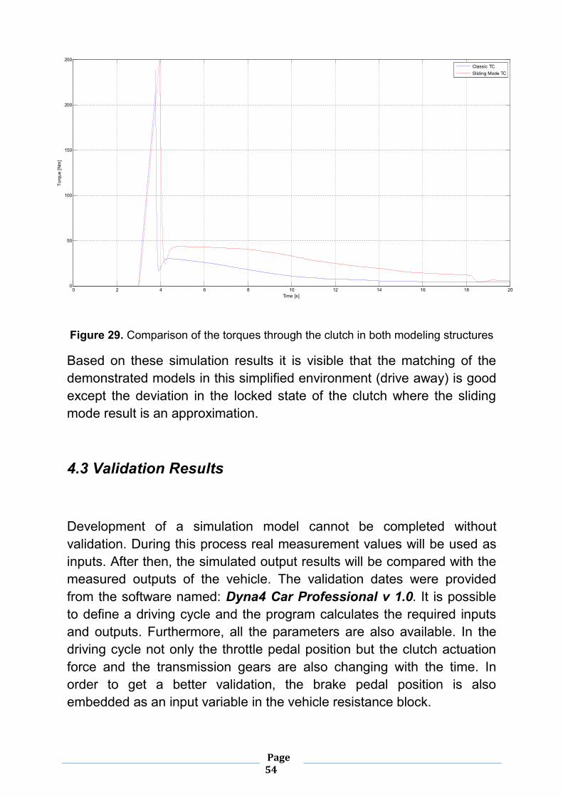
It is visible that the results are similar to the classical solution. The chattering effect is also eliminated with a saturation block so there is no need to filter the chattered signal with a low-pass filter. In the fifth sub-plot of the Figure 28 the torques from the engine and the clutch are depicted. Figure 29 compares the torque through the clutch cT with the torque calculated in the classical solution.
0 2 4 6 8 10 12 14 16 18 20
0
200
400
600
Time [s]
Vel
ocity
[rad
/s]
Drive Away Simulation Sliding Mode Model
Engine SpeedClutch Speed
0 2 4 6 8 10 12 14 16 18 200
20
40
Time [s]
Spe
ed [k
m/s
]
Vehicle Speed
0 2 4 6 8 10 12 14 16 18 200
100
200
300
Time [s]
Torq
ue [N
m]
Clutch Torque ChatteringClutch Torque Filtered
0 2 4 6 8 10 12 14 16 18 200
100
200
300
Time [s]
Torq
ue [N
m]
Engine TorqueClutch Torque
Page 54
Figure 29. Comparison of the torques through the clutch in both modeling structures
Based on these simulation results it is visible that the matching of the demonstrated models in this simplified environment (drive away) is good except the deviation in the locked state of the clutch where the sliding mode result is an approximation.
4.3 Validation Results
Development of a simulation model cannot be completed without validation. During this process real measurement values will be used as inputs. After then, the simulated output results will be compared with the measured outputs of the vehicle. The validation dates were provided from the software named: Dyna4 Car Professional v 1.0. It is possible to define a driving cycle and the program calculates the required inputs and outputs. Furthermore, all the parameters are also available. In the driving cycle not only the throttle pedal position but the clutch actuation force and the transmission gears are also changing with the time. In order to get a better validation, the brake pedal position is also embedded as an input variable in the vehicle resistance block.
0 2 4 6 8 10 12 14 16 18 200
50
100
150
200
250
Time [s]
Torq
ue [N
m]
Classic TCSliding Mode TC

Page 55
The initial conditions are exact the same as in the drive away simulation. The vehicle starts from standstill in a road with a slope of o0 . The same validation values were used in both modeling constructions. Figure 30 collects the input variables of the simulation.
Figure 30. Input variables of the validation simulation in both modeling concepts
The simulation lasts sec100 and the integration step size is 1 ms . Figures 31 and 32 are presenting the validation results of the classical- and the sliding mode model respectively. In both figures the first sub-plot shows the engine torque, the second displays the engine angular velocity, the third shows the vehicle speed and finally the fourth sub-plot presents the throttle- and brake pedal positions. It is apparent the matching is good in both modeling concepts. In order to decide which model provides a better accuracy Figure 36 presents the error function of the simulated results in the same plot. The error function means the deviation of the simulated value from the measured value. The first sub-plot presents the deviation of the engine torque, the second depicts the engine angular velocity and the third shows the deviation of the vehicle speed.
0 10 20 30 40 50 60 70 80 90 100
0
20
40
60
80
100
Time [s]
Pos
ition
[%]
Throttle Pedal PositionBrake Pedal Position
0 10 20 30 40 50 60 70 80 90 100
0
0.5
1
Time [s]
Pos
ition
[%]
Clutch Pedal Position
0 10 20 30 40 50 60 70 80 90 100-1
0
1
2
3
4
Time [s]
Gea
r
Actual Gear Ratio

Page 56
Figure 31. The validation results of the classical solution with measured data
Figure 32. The validation results of the sliding mode model with measured data
0 10 20 30 40 50 60 70 80 90 100-100
0
100
200
Time [s]
Torq
ue [N
m]
Simulation Result Classical Solution
Engine Torque SimulatedEngine Torque Measured
0 10 20 30 40 50 60 70 80 90 1000
2000
4000
6000
Time [s]
Ang
ular
Vel
ocity
[RP
M]
Engine Speed SimulatedEngine Speed Measured
0 10 20 30 40 50 60 70 80 90 1000
50
100
150
Time [s]
Spe
ed [k
m/h
]
Vehicle Speed SimulatedVehicle Speed Measured
0 10 20 30 40 50 60 70 80 90 1000
50
100
Time [s]
Pos
ition
[%]
Throttle Pedal PositionBrake Pedal Position
0 10 20 30 40 50 60 70 80 90 100-100
0
100
200
Time [s]
Torq
ue [N
m]
Simulationsergebnisse
Engine Torque SimEngine Torque Soll
0 10 20 30 40 50 60 70 80 90 1000
2000
4000
6000
Time [s]
RP
M
Motor Speed SimMotor Speed Soll
0 10 20 30 40 50 60 70 80 90 1000
50
100
150
Time [s]
km/h
Vehicle Speed SimVehicle Speed Soll
0 10 20 30 40 50 60 70 80 90 1000
50
100
Time [s]
Pos
ition
[%]
FahrpedalBremspedal

Page 57
Another important signal to calculate is the torque through the clutch. As been mentioned in the drive away simulation the behavior of the sliding mode model can be influenced by the chattering effect when the clutch is locked. The same behavior is expected in the validation. Figure 34 shows, how the chattering phenomena influences the torque through the clutch in the sliding mode model when the sign function is used. However, this effect is eliminated with a saturation block and the comparison is plotted in Figure 35. Similar to the drive away simulation the matching is also good with a deviation in the locked phase of the clutch.
Figure 34. The torque TC chattering phenomenon in the sliding mode model compared with the filtered signal
0 10 20 30 40 50 60 70 80 90 100-400
-300
-200
-100
0
100
200
300
400
Time [s]
Torq
ue [N
m]
Torque TC without FilteringTorque TC with Filtering

Page 58
Figure 35. Comparison of the torque through the clutch TC in classical- and sliding mode model
These results are proved that the dynamic behavior of the sliding mode model is similar to the classical solution in a more complex driving cycle. With these results the validation is successfully completed.
0 10 20 30 40 50 60 70 80 90 100-300
-200
-100
0
100
200
300
Time [s]
Torq
ue [N
m]
Classic TCSliding Mode TC

Page 59
Figure 36. Deviation functions of the engine torque, velocity and the vehicle speed
0 10 20 30 40 50 60 70 80 90 1000
20
40
60
80
Time [s]
Torq
ue [N
m]
Engine Torque Error ClassicEngine Torque Error Sliding Mode
0 10 20 30 40 50 60 70 80 90 1000
50
100
150
Time [s]
Ang
ular
Vel
ocity
[rad
/s]
Engine Velocity Error ClassicEngine Velocity Error Sliding Mode
0 10 20 30 40 50 60 70 80 90 1000
5
10
15
Time [s]
Veh
icle
Spe
ed [k
m/h
]
Vehicle Speed Error ClassicVehicle Speed Error Sliding Mode

Page 60
5 Conclusions and Future Work In the Master Thesis, the difficulty of finding a simple and realistic simulation model for an automotive powertrain system has been presented. During the modeling, the greatest problem represents the clutch element. Depending on the state of the clutch (slip, stick), different motion equations are describing the dynamic behavior of this element. Variable system dimension, i.e. changing degrees of freedom, and discontinuous transitions are challenging issues in the simulation to be treated. For simulating this type of systems, in the literature one can find rather complex models (classical solution), or approximated models (sliding mode models) that give rough results. Within the scope of this thesis, both concepts are developed in MATLAB/Simulink, compared to each other, and validated using synthetic and measurement data. Simulation results showed that the dynamic behavior of the implemented concepts is in accordance whereas all of the required signals stated in the problem formulation of the thesis are calculated. Concerning the modularity, the constructed models are not the optimal solutions. Modularity can be further increased with a performance-based modeling. Another opportunity for further development of the models is to determine and to quantify the parameter uncertainties. Modeling of additional effects of certain powertrain elements, like temperature dependency, is also part of future improvements.

Page 61
6 References
[1] The Lubrizol Corporation (2008 - 2011), Wet clutch or dry clutch? Available: http://www.dctfacts.com/information/wet-clutch-or-dry-clutch.aspx. Last accessed 22/10/2011.
[2] OSX (16/10/2010). Subaru Liberty powertrain. Available: http://en.wikipedia.org/wiki/File:Subaru_Liberty_powertrain_%282010-10-16%29.jpg. Last accessed: 22/10/2011.
[3] L. Guzzella, A. Sciarretta Vehicle Propulsion Systems, Springer – Verlag Berlin Heidelberg, pp. 41- 45, 2005
[4] R. Zanasi, G. Sandoni, R. Morselli Simulation of variable dynamic dimension systems: The clutch example, European Control Conference, 2001
[5] Mathworks Demo, Building a Clutch Lock-Up model with MATLAB version R2010b, http://www.mathworks.de/products/simulink/demos.html?file=/products/demos/shipping/simulink/sldemo_clutch.html, Last accessed: 29/11/2011
[6] J. H. Taylor Rigorous Handling of State Events in MATLAB, IEEE International Conference on Control Application, pp. 156-161, 1995
[7] M. V. Datar Powertrain Systems in ADAMS/Car, University of Wisconsin, 2007
[8] A. Serrarens, M. Dassen, M. Steinbuch Simulation and Control of an Automotive Dry Clutch, American Control Conference Boston, 2004
[9] K. Gopinath, M. M. Mayuram Machine Design II-Clutch, Indian Institute of Technology Madras, Lecture Notes to the class Machine Design II, http://nptel.iitm.ac.in/courses/IIT-MADRAS/Machine_Design_II/pdf/3_5.pdf
[10] H. J. Draxl Motor Vehicles Clutches, Verlag Moderne Industrie,1998
[11] Motorera Dictionary. Available: http://www.motorera.com/dictionary/pics/d/diaphragm_clutch.jpg . Last accessed: 23/10/2011.
[12] Math Works Homepage http://www.mathworks.de/help/toolbox/simulink/ug/f11-69449.html#f11-41861 Last accessed: 29/11/2011

Page 62
[13] H. Naunheimer, B. Bertsche, J. Ryborz, W. Novak Automotive Transmissions, Springer-Verlag Berlin Heidelberg, 1994
[14] Übungsfolie zu Lehrveranstaltung: Simulation mit Simulink/Matlab,TU München, http://www.eal.ei.tum.de/lehre/ssm/folien_simulink_grund.pdf, Last accessed: 29/11/2011
[15] Dyna4 Homepage. Available: http://tesis-dynaware.com/en/products/car-professional/overview-benefits.html. Last accessed: 29.11.2011
[16] G. Sandoni, Modeling and control of a car driveline, PHD in Information Engineering at the University of Modena and Reggio Emilia, Chapter 4, pp. 33-45, 2002
[17] M. Mitschke, H. Wallentowitz, Dynamik der Kraftfahrzeuge, Springer - Verlag, Auflage 4, 2003
[18] V. I. Utkin Sliding Mode Control Design Principles and Applications to Eletric Drives, IEEE Trans. on Industrial Electronics, Vol. 40, No. 1, 1993
[19] S. V. Drakunov, Ü.Özgüner, P.Dix and B.Ashrafi ABS Control using optimum search via sliding modes, IEEE Transaction on Control Systems Technology, Vol. 3, pp. 79-85, 1995
[20] S. V.Drakunov, D. Hanchin, W-C. Su and Ü. Özgüner Nonlinear control of a rodless pneumatic servoactuator or sliding modes versus coulomb friction, Automatica, Vol.33, No. 7, pp.1401-1406, 1997
[21] R. Isermann Mechatronische Systeme (Grundlagen), Springer, pp. 47-51, 2008
[22] V. I. Utkin Variable Structure Systems with Sliding Modes, IEEE Trans. Automatic Control, Vol. 22, 1977
[23] A. Hofer Modellierung Mechatronischer Systeme, Skriptum zur Lehrveranstalung Modellierung Mechatronischer Systeme an der TU Graz bei Institut für Regelungs- und Automatisierungstechnik, 2005
[24] H. J. Bartsch Mathematischer Formeln, Fachbuchverlag Leipzig, Auflage 21, 2007