maximal function and multiplier theorem for weighted space ...dfeng/jfa07.pdf · 478 f. dai, y. xu...
TRANSCRIPT

Journal of Functional Analysis 249 (2007) 477–504
www.elsevier.com/locate/jfa
Maximal function and multiplier theorem for weightedspace on the unit sphere ✩
Feng Dai a,∗, Yuan Xu b
a Department of Mathematical and Statistical Sciences, University of Alberta, Edmonton, Alberta T6G 2G1, Canadab Department of Mathematics, University of Oregon, Eugene, OR 97403-1222, USA
Received 3 December 2006; accepted 26 March 2007
Available online 4 May 2007
Communicated by G. Pisier
Abstract
For a family of weight functions invariant under a finite reflection group, the boundedness of a maximalfunction on the unit sphere is established and used to prove a multiplier theorem for the orthogonal ex-pansions with respect to the weight function on the unit sphere. Similar results are also established for theweighted space on the unit ball and on the standard simplex.© 2007 Elsevier Inc. All rights reserved.
Keywords: Maximal function; Multiplier; h-Harmonics; Sphere; Orthogonal polynomials; Ball; Simplex
1. Introduction
The purpose of this paper is to study the maximal function in the weighted spaces on theunit sphere and the related domains. Let Sd = {x: ‖x‖ = 1} be the unit sphere in R
d+1, where‖x‖ denotes the usual Euclidean norm. Let 〈x, y〉 denote the usual Euclidean inner product. We
✩ The first author was partially supported by the NSERC Canada under grant G121211001. The second author waspartially supported by the National Science Foundation under Grant DMS-0604056.
* Corresponding author.E-mail addresses: [email protected] (F. Dai), [email protected] (Y. Xu).
0022-1236/$ – see front matter © 2007 Elsevier Inc. All rights reserved.doi:10.1016/j.jfa.2007.03.023

478 F. Dai, Y. Xu / Journal of Functional Analysis 249 (2007) 477–504
consider the weighted space on Sd with respect to the measure h2κ dω, where dω is the surface
(Lebesgue) measure on Sd and the weight function hκ is defined by
hκ(x) =∏
v∈R+
∣∣〈x, v〉∣∣κv , x ∈ Rd+1, (1.1)
in which R+ is a fixed positive root system of Rd+1, normalized so that 〈v, v〉 = 2 for all v ∈ R+,
and κ is a nonnegative multiplicity function v �→ κv defined on R+ with the property that κu = κv
whenever σu, the reflection with respect to the hyperplane perpendicular to u, is conjugate to σv
in the reflection group G generated by the reflections {σv: v ∈ R+}. The function hκ is invariantunder the reflection group G. The simplest example is given by the case G = Z
d+12 for which hκ
is just the product weight function
hκ(x) =d+1∏i=1
|xi |κi , κi � 0, x = (x1, . . . , xd+1). (1.2)
Denote by aκ the normalization constant, a−1κ = ∫
Sd h2κ(y) dω(y). We consider the weighted
space Lp(h2κ ;Sd) of functions on Sd with the finite norm
‖f ‖κ,p :=(
aκ
∫Sd
∣∣f (y)∣∣ph2
κ(y) dω(y)
)1/p
, 1 � p < ∞,
and for p = ∞ we assume that L∞ is replaced by C(Sd), the space of continuous functions onSd with the usual uniform norm ‖f ‖∞.
The weight function (1.1) was first studied by Dunkl in the context of h-harmonics, which areorthogonal polynomials with respect to h2
κ . A homogeneous polynomial is called an h-sphericalharmonics if it is orthogonal to all polynomials of lower degree with respect to the inner productof L2(h2
κ ;Sd). The theory of h-harmonics is in many ways parallel to that of ordinary harmonics(see [5]). In particular, many results on the spherical harmonics expansions have been extendedto h-harmonics expansions, see [3–5,8,12,13] and the references therein. Much of the analysisof h-harmonics depends on the intertwining operator Vκ that intertwines between Dunkl opera-tors, which are a commuting family of first order differential–difference operators, and the usualpartial derivatives. The operator Vκ is a uniquely determined positive linear operator. To seethe importance of this operator, let Hd+1
n (h2κ ) denote the space of h-harmonics of degree n; the
reproducing kernel of Hd+1n (h2
κ ) can be written in terms of Vκ as
P hn (x, y) = n + λk
λκ
Vκ
[Cλk
n
(〈x, ·〉)](y), x, y ∈ Sd, (1.3)
where Cλn is the nth Gegenbauer polynomial, which is orthogonal with respect to the weight
function wλ(t) := (1 − t2)λ−1/2 on [−1,1], and
λκ = γκ + d − 1
2with γκ =
∑κv. (1.4)
v∈R+

F. Dai, Y. Xu / Journal of Functional Analysis 249 (2007) 477–504 479
Furthermore, using Vκ , a maximal function that is particularly suitable for studying the h-harmonic expansion is defined in [13] by
Mκf (x) := sup0<θ�π
∫Sd |f (y)|Vκ [χB(x,θ)](y)h2
κ (y) dω(y)∫Sd Vκ [χB(x,θ)](y)h2
κ (y) dω(y), (1.5)
where B(x, θ) := {y ∈ Bd+1: 〈x, y〉 � cos θ}, Bd+1 := {x: ‖x‖ � 1} ⊂ Rd+1, and χE denotes
the characteristic function of the set E. A weak type (1,1) inequality was established for Mκf
in [13]. The result, however, is weaker than the usual weak type (1,1) inequality and it doesnot imply the strong (p,p) inequality. One of our main results in this paper is to establish agenuine weak type (1,1) result, for which we rely on the general result of [9] on semi-groups ofoperators. Furthermore, the Fefferman–Stein type result∥∥∥∥(∑
j
|Mκfj |2)1/2∥∥∥∥
κ,p
� c
∥∥∥∥(∑j
|fj |2)1/2∥∥∥∥
κ,p
also holds, which can be used to derive a multiplier theorem for h-harmonic expansions, follow-ing the approach of [1]. These results are presented in Section 2.
In the case of Zd+12 , the explicit formula of Vκ as an integral operator is known, which allows
us to link the maximal function Mκf with the weighted Hardy–Littlewood maximal functiondefined by
Mkf (x) := sup0<θ�π
∫c(x,θ)
|f (y)|h2κ (y) dω(y)∫
c(x,θ)h2
κ (y) dω(y), (1.6)
where c(x, θ) := {y ∈ Sd : 〈x, y〉 � cos θ} is the spherical cap. We will show that the maximalfunction Mκf is bounded by a sum of the Hardy–Littlewood maximal function Mκf . As aconsequence, we establish a weighted weak (1,1) result for Mkf (x), in which the weight isalso of the form (1.2) but with different parameters. Furthermore, we show that the Fefferman–Stein type inequality holds in the weighted Lp norm. These results are discussed in Section 3.
The analysis on the sphere is closely related to the analysis on the unit ball Bd and on thestandard simplex T d . In fact, much of the results on the later two cases can be deduced from thoseon the sphere (see [5,12,13] and the references therein). In particular, maximal functions are alsodefined on Bd and T d in terms of the generalized translation operators [13]. We will extend ourresults on the sphere in Section 2 to these two domains, including a multiplier theorem for theorthogonal expansions in the weighted space on Bd and T d , in Sections 4 and 5, respectively.
Throughout this paper, the constant c denotes a generic constant, which depends only on thevalues of d , κ and other fixed parameters and whose value may be different from line to line.Furthermore, we write A ∼ B if A � cB and B � cA.
2. Maximal function and multiplier theorem on Sd
2.1. Background
In this subsection we give a brief account of what will be needed later on in the paper. Formore background and details, we refer to [5,12,13].

480 F. Dai, Y. Xu / Journal of Functional Analysis 249 (2007) 477–504
h-Harmonic expansion. Let Hd+1n (h2
κ ) denote the space of spherical h-harmonics of degree n.It is known that dimHd+1
n (h2κ ) = (
n+d+1n
) − (n+d−1
n−2
). The usual Hilbert space theory shows that
L2(h2k;Sd
) =∞∑
n=0
Hd+1n
(h2
κ
): f =
∞∑n=0
projκn f,
where projκn :L2(h2κ ;Sd) �→ Hd+1
n (h2κ ) is the projection operator, which can be written as an
integral operator
projκn f (x) = aκ
∫Sd
f (y)P hn (x, y)h2
κ (y) dω(y), (2.1)
where P hn is the reproducing kernel of Hd+1
n (h2κ ), which satisfies the compact representa-
tion (1.3).
Intertwining operator. For a general reflection group, the explicit formula of Vκ is not known.In the case of Z
d+12 , it is an integral operator given by
Vκf (x) = cκ
∫[−1,1]d+1
f (x1t1, . . . , xd+1td+1)
d+1∏i=1
(1 + ti )(1 − t2
i
)κi−1dt, (2.2)
where cκ is the normalization constant determined by Vκ1 = 1. If some κi = 0, then the formulaholds under the limit relation
limλ→0
cλ
1∫−1
f (t)(1 − t)λ−1 dt = [f (1) + f (−1)
]/2.
Convolution. For f ∈ L1(h2κ ;Sd) and g ∈ L1(wλκ ; [−1,1]), define [12, Definition 2.1, p. 6]
f κ g(x) := aκ
∫Sd
f (y)Vκ
[g(〈x, ·〉)](y)h2
κ (y) dω(y). (2.3)
This convolution satisfies the usual Young’s inequality (see [12, Proposition 2.2, p. 6]): forf ∈ Lq(h2
κ ;Sd) and g ∈ Lr(wλκ ; [−1,1]), ‖f κ g‖k,p � ‖f ‖k,q‖g‖wλκ ,r , where p,q, r � 1and p−1 = r−1 + q−1 − 1. For κ = 0, Vκ = id , this becomes the classical convolution on thesphere [2]. Notice that by (1.3) and (2.1), we can write projκn f as a convolution.
Cesàro (C, δ) means. For δ > 0, the (C, δ) means, sδn, of a sequence {cn} are defined by
sδn = (
Aδn
)−1n∑
Aδn−kck, Aδ
n−k =(
n − k + δ
n − k
).
k=0

F. Dai, Y. Xu / Journal of Functional Analysis 249 (2007) 477–504 481
We denote the nth (C, δ) means of the h-harmonic expansion by Sδn(h
2κ ;f ). These means can be
written as
Sδn
(h2
κ ;f ) = (f κ qδ
n
)(x), qδ
n(t) = (Aδ
n
)−1n∑
k=0
Aδn−k
(k + λ)
λCλ
k (t),
where λ = λκ . The function qδn(t) is the kernel of the (C, δ) means of the Gegenbauer expansions
at x = 1.
Generalized translation operator T κθ . This operator is defined implicitly by [12, p. 7]
cλ
π∫0
T κθ f (x)g(cos θ)(sin θ)2λ dθ = (f κ g)(x), (2.4)
where g is any L1(wλ) function and λ = λκ . The operator T κθ is well defined and becomes the
classical spherical means
Tθf (x) = 1
σd(sin θ)d−1
∫〈x,y〉=cos θ
f (y) dω(y),
when κ = 0, where σd = ∫Sd−1 dω = 2πd/2/�(d/2) is the surface area of Sd−1. Furthermore,
T κθ satisfies similar properties as those satisfied by Tθ , as shown in [12,13]. In particular, if
f (x) = 1, then T κθ f (x) = 1.
Spherical caps. Let d(x, y) := arccos 〈x, y〉 denote the geodesic distance of x, y ∈ Sd . For0 � θ � π , the set
c(x, θ) := {y ∈ Sd : d(x, y) � θ
} = {y ∈ Sd : 〈x, y〉 � cos θ
}is called the spherical cap centered at x. Sometimes we need to consider the solid set under thespherical cap, which we denote by B(x, θ) to distinguish it from c(x, θ); that is,
B(x, θ) := {y ∈ Bd+1: 〈x, y〉 � cos θ
},
where Bd+1 = {y ∈ Rd+1: ‖y‖ � 1}.
Maximal function. For f ∈ L1(h2κ ), define [13]
Mκf (x) := sup0<θ�π
∫ θ
0 T κφ |f |(x)(sinφ)2λκ dφ∫ θ
0 (sinφ)2λκ dφ.
This maximal function can be used to study the h-harmonic expansions, since we can often prove|(f κ g)(x)| � cMκf (x). Using (2.4) it is shown in [13] that an equivalent definition for Mκf
is (1.5); that is,
Mκf (x) = sup
∫Sd |f (y)|Vκ [χB(x,θ)](y)h2
κ (y) dω(y)∫d Vκ [χB(x,θ)](y)h2(y) dω(y)
. (2.5)
0<θ�π S κ
482 F. Dai, Y. Xu / Journal of Functional Analysis 249 (2007) 477–504
We note that setting f (x) = 1 and g(t) = χ[cos θ,1](t) in (2.4) leads to
aκ
∫Sd
Vκ [χB(x,θ)](y)h2κ (y) dω(y) = cλκ
θ∫0
(sinφ)2λκ dφ ∼ θ2λκ+1. (2.6)
2.2. Maximal function
To state the weak type inequality, we define, for any measurable subset E of Sd , the measurewith respect to h2
κ as
measκ E :=∫E
h2κ(y) dω(y).
Our main result in this section is the boundeness of Mκf .
Theorem 2.1. If f ∈ L1(h2κ ;Sd), then Mκf satisfies
measκ
{x: Mκf (x) � α
}� c
‖f ‖κ,1
α, ∀α > 0. (2.7)
Furthermore, if f ∈ Lp(h2κ ;Sd) for 1 < p � ∞, then ‖Mkf ‖κ,p � c‖f ‖κ,p .
The inequality (2.7) is usually refereed to as weak type (1,1) inequality. In order to provethis theorem, we follow the approach of [9] on general diffusion semi-groups of operators on ameasure space. For this we need the Poisson integral with respect to h2
κ , which can be written as[5, Theorem 5.3.3, p. 190]
P κr f (x) = f κ pκ
r , where pκr (s) = 1 − r2
(1 − 2rs + r2)λk+1. (2.8)
The kernel pκr is one of the generating function of the Gegenbauer polynomials of parameter λκ .
Hence, by (1.3), we can write P κr f as
P κr f (x) =
∞∑n=0
rn projκn f (x), 0 � r < 1,
from which it follows easily that T t := P κr f with r = e−t defines a semi-group. Since Vκ is
positive and pκr is clearly non-negative, P κ
r f � 0 if f � 0. We see that the semi-group P κe−t f is
positive. We will need another semi-group, which is the discrete analog of the heat operator:
Hκt f := f κ qκ
t , qκt (s) :=
∞∑e−n(n+2λκ )t n + λκ
λκ
Cλκn (s). (2.9)
n=0

F. Dai, Y. Xu / Journal of Functional Analysis 249 (2007) 477–504 483
In fact, the h-harmonics in Hd+1n (h2
κ ) are the eigenfunctions of an operator �h,0, which is thespherical part of a second order differential–difference operator analogous to the ordinary Lapla-cian, the eigenvalues are −n(n + 2λk). It follows immediately from (2.9) that {Hκ
t }t�0 is asemi-group. The following result is the key for the proof of the theorem.
Lemma 2.2. The Poisson and the heat semi-groups are connected by
P κe−t f (x) =
∞∫0
φt (s)Hκs f (x) ds, (2.10)
where
φt (s) := t
2√
πs−3/2e
−( t2√
s−λκ
√s )2
.
Furthermore, assume that f (x) � 0 for all x, then for all t > 0,
P κ∗ f (x) := sup0<r<1
P κr f (x) � c sup
s>0
1
s
s∫0
Hκu f (x)du. (2.11)
Consequently, P κ∗ f is bounded on Lp(h2κ ;Sd) for 1 < p � ∞ and of weak type (1,1).
Proof. That {Hκt }t�0 is a semi-group is obvious. Moreover, since Vκ is positive and qκ
t is knownto be non-negative [7], it follows that Hκ
t f is positive. The positivity shows that ‖qκt ‖wλκ ,1 = 1,
so that ‖Hκt f ‖κ,p � ‖f ‖κ,p , 1 � p � ∞, by applying Young’s inequality on f κ qκ
t . Thus,using the Hopf–Dunford–Schwarz ergodic theorem [9, p. 48], we conclude that the maximaloperator sups>0(
1s
∫ s
0 Hκu f (x)du) is bounded on Lp(h2
κ ;Sd) for 1 < p � ∞ and of week type(1,1). Therefore, it is sufficient to prove (2.10) and (2.11).
First we prove (2.10). Applying the well-known identity [9, p. 46]
e−v = 1√π
∞∫0
e−u
√u
e− v24u du, v > 0,
with v = (n + λκ)t and making a change of variable s = t2/4u, we conclude that
e−nt = eλκ t 1√π
∞∫0
e−u
√u
e− n(n+2λκ )t24u e− λ2
κ t2
4u du
= t
2√
π
∞∫0
e−n(n+2λκ )ss−3/2e−( t
2√
s−λκ
√s )2
ds
=∞∫
0
e−n(n+2λκ )sφt (s) ds.
Multiplying by projκn f and summing up over n proves the integral relation (2.10).

484 F. Dai, Y. Xu / Journal of Functional Analysis 249 (2007) 477–504
For the proof of (2.11), we use (2.10) and integration by parts to obtain
P κe−t f (x) = −
∞∫0
( s∫0
Hκu f (x)du
)φ′
t (s) ds
� sups>0
(1
s
s∫0
Hκu f (x)du
) ∞∫0
s∣∣φ′
t (s)∣∣ds,
where the derivative of φ′t (s) is taken with respect to s. Also, we note that by (2.8) and (2.3),
sup0<r�e−1
P κr f (x) � c‖f ‖1,κ = c lim
s→∞1
s
s∫0
Hκu
(|f |)(x) du.
Therefore, to finish the proof of (2.11), it suffices to show that sup0<t�1
∫ ∞0 s|φ′
t (s)|ds isbounded by a constant.
A quick computation shows that φ′t (s) > 0 if s < αt and φ′
t (s) < 0 if s > αt , where
αt := t2
3 + √9 + 4λ2
κ t2∼ t2, 0 � t � 1.
Since the integral of φt (s) over [0,∞) is 1 and φt (s) � 0, integration by parts gives
∞∫0
s∣∣φ′
t (s)∣∣ds = 2αtφt (αt ) −
αt∫0
φt (s) ds +∞∫
αt
φt (s) ds
� 2αtφt (αt ) + 1 = t√παt
e− (t−2λκ αt )
2
4αt + 1 � c
as desired. �We are now in a position to prove Theorem 2.1.
Proof of Theorem 2.1. From the definition of pκr , it follows easily that if 1 − r ∼ θ , then
pκr (cos θ) = 1 − r2
((1 − r)2 + 4r sin2 θ2 )λκ+1
� c1 − r2
((1 − r)2 + rθ2)λκ+1� c (1 − r)−(2λκ+1).
For j � 0 define rj := 1 − 2−j θ and set Bj := {y ∈ Bd+1: 2−j−1θ � d(x, y) � 2−j θ}. Thelower bound of pκ
r proved above shows that
χBj(y) � c
(2−j θ
)2λk+1pκ
r
(〈x, y〉),
j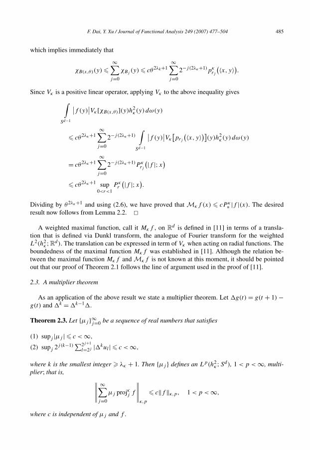
F. Dai, Y. Xu / Journal of Functional Analysis 249 (2007) 477–504 485
which implies immediately that
χB(x,θ)(y) �∞∑
j=0
χBj(y) � cθ2λk+1
∞∑j=0
2−j (2λκ+1)pκrj
(〈x, y〉).Since Vκ is a positive linear operator, applying Vκ to the above inequality gives∫
Sd−1
∣∣f (y)∣∣Vκ [χB(x,θ)](y)h2
κ (y) dω(y)
� cθ2λκ+1∞∑
j=0
2−j (2λκ+1)
∫Sd−1
∣∣f (y)∣∣Vκ
[prj
(〈x, y〉)](y)h2κ (y) dω(y)
= cθ2λκ+1∞∑
j=0
2−j (2λκ+1)P κrj
(|f |;x)� cθ2λκ+1 sup
0<r<1P κ
r
(|f |;x).
Dividing by θ2λκ+1 and using (2.6), we have proved that Mκf (x) � cP κ∗ |f |(x). The desiredresult now follows from Lemma 2.2. �
A weighted maximal function, call it Mκf , on Rd is defined in [11] in terms of a transla-
tion that is defined via Dunkl transform, the analogue of Fourier transform for the weightedL2(h2
κ ;Rd). The translation can be expressed in term of Vκ when acting on radial functions. The
boundedness of the maximal function Mκf was established in [11]. Although the relation be-tween the maximal function Mκf and Mκf is not known at this moment, it should be pointedout that our proof of Theorem 2.1 follows the line of argument used in the proof of [11].
2.3. A multiplier theorem
As an application of the above result we state a multiplier theorem. Let �g(t) = g(t + 1) −g(t) and �k = �k−1�.
Theorem 2.3. Let {μj }∞j=0 be a sequence of real numbers that satisfies
(1) supj |μj | � c < ∞,
(2) supj 2j (k−1)∑2j+1
l=2j |�kul | � c < ∞,
where k is the smallest integer � λκ + 1. Then {μj } defines an Lp(h2κ ;Sd), 1 < p < ∞, multi-
plier; that is, ∥∥∥∥∥∞∑
j=0
μj projκj f
∥∥∥∥∥κ,p
� c‖f ‖κ,p, 1 < p < ∞,
where c is independent of μj and f .

486 F. Dai, Y. Xu / Journal of Functional Analysis 249 (2007) 477–504
When κ = 0, the theorem becomes part of [1, Theorem 4.9] on the ordinary spherical har-monic expansions. The proof of this theorem follows that of the theorem in [1]. One of the mainingredient is the Littlewood–Paley function
g(f ) =( 1∫
0
(1 − r)
∣∣∣∣ ∂
∂rP κ
r f
∣∣∣∣2
dr
)1/2
, (2.12)
where P κr f is the Poisson integral with respect to h2
κ defined in (2.8). A general Littlewood-Paley theory was established in [9] for a family of diffusion semi-group of operators {T t }t�0 ona measure space, in which the g function is defined as
g1(f ) =( ∞∫
0
t
∣∣∣∣ ∂
∂tT tf
∣∣∣∣2
dt
)1/2
.
Applying the general theory to T t := P κr f with r = e−t and using the fact that the crucial point
in the definition of g(f ) is when r close to 1, it follows that
c−1‖f ‖κ,p �∥∥g(f )
∥∥κ,p
� c‖f ‖κ,p, 1 < p < ∞, (2.13)
for f ∈ Lp(h2κ ;Sd), where the inequality in the left-hand side holds under the additional assump-
tion that∫Sd f (y)h2
κ (y) dy = 0. Another ingredient of the proof is the Cesàro means. Recall thatthe (C, δ) means are denoted by Sδ
n(h2κ ;f ). What is needed is the following result.
Theorem 2.4. For δ > λκ , 1 < p < ∞ and any sequence {nj } of positive integers,
∥∥∥∥∥( ∞∑
j=0
∣∣Sδnj
(h2
κ ;fj
)∣∣2
)1/2∥∥∥∥∥κ,p
� c
∥∥∥∥∥( ∞∑
j=0
∣∣fj
∣∣2
)1/2∥∥∥∥∥κ,p
. (2.14)
Proof. The proof of (2.14) follows the approach of [9, pp. 104–105] that uses a generalizationof the Riesz convexity theorem for sequences of functions. Let Lp(�q) denote the space of allsequences {fk} of functions for which the norm
∥∥(fk)∥∥
Lp(�q
) :=( ∫
Sd
( ∞∑j=0
∣∣fj (x)∣∣q)p/q
h2κ (x) dω(x)
)1/p
is finite. If T is bounded as operator on Lp0(�q0) and on Lp1(�q1), then the Riesz convexitytheorem states that T is also bounded on Lpt (�qt ), where
1 = 1 − t + t,
1 = 1 − t + t, 0 � t � 1.
pt p0 p1 qt q0 q1

F. Dai, Y. Xu / Journal of Functional Analysis 249 (2007) 477–504 487
We apply this theorem on the operator T that maps the sequence {fj } to the sequence{Sδ
nj(h2
κ ;fj )}. It is shown in [13, pp. 76 and 78] that supn|Sδn(h
2κ ;f )(x)| � cMκf (x) for all
x ∈ Sd if δ > λκ . Consequently, T is bounded on Lp(�p). It is also bounded on Lp(�∞) since∥∥∥supj�0
∣∣Sδnj
(h2
κ ;fj
)∣∣∥∥∥κ,p
� c
∥∥∥Mκ
(supj�0
|fj |)∥∥∥
κ,p� c
∥∥∥supj�0
|fj |∥∥∥
κ,p.
Hence, the Riesz convexity theorem shows that T is bounded on Lp(�q) if 1 < p � q � ∞. Inparticular, T is bounded on Lp(�2) if 1 < p � 2. The case 2 < p < ∞ follows by the standardduality argument, since the dual space of Lp(�2) is Lp′
(�2), where 1/p + 1/p′ = 1, under theparing
⟨(fj ), (gj )
⟩ := ∫Sd
∑j
fj (x)gj (x)h2κ (x) dω(x)
and T is self-adjoint under this paring as Sδn(h
2κ ) is self-adjoint in L2(h2
κ ;Sd). �Using the two ingredients, (2.13) and (2.14), the proof of Theorem 2.3 follows from the cor-
responding proof in [1] almost verbatim.
Remark 2.1. In the case of κ = 0, the condition δ > λκ = (d − 1)/2 is the critical index forthe convergence of (C, δ) means in Lp(h2
κ ;Sd) for all 1 � p � ∞. For h2κ given in (1.2) and
G = Zd2 , this remains true if at least one κi is zero. However, if κi �= 0 for all i, then the critical
index is λκ −min1�i�d+1 κi [8]. It remains to be seen if the condition k � λκ +1 in Theorem 2.3can be improved to k � λκ − min1�i�d+1 κi + 1.
The proof of Theorem 2.4 actually yields the following Fefferman–Stein type inequality [6]for the maximal function Mκf .
Corollary 2.5. Let 1 < p � 2 and fj be a sequence of functions. Then∥∥∥∥(∑j
(Mκfj )2)1/2∥∥∥∥
κ,p
� c
∥∥∥∥(∑j
|fj |2)1/2∥∥∥∥
κ,p
. (2.15)
We do not know if the inequality (2.15) holds for 2 < p < ∞ under a general finite reflectiongroup. However, it will be shown in the next section that (2.15) is true for all 1 < p < ∞ in thecase of G = Z
d+12 .
3. Maximal function for product weight
The result on the maximal function in the previous section is established for every finitereflection group. In the case of G = Z
d+12 , the weight function becomes (1.2); that is,
hκ(x) =d+1∏
|xi |κi , κi � 0.
i=1

488 F. Dai, Y. Xu / Journal of Functional Analysis 249 (2007) 477–504
We know the explicit formula of the intertwining operator Vκ , as shown in (2.2). This additionalinformation turns out to offer more insight into the maximal function Mkf . The main result inthis section relates Mκf to the weighted Hardy–Littlewood maximal function.
Definition 3.1. For f ∈ L1(h2κ ;Sd), the weighted Hardy–Littlewood maximal function is defined
by
Mκf (x) := sup0<θ�π
∫c(x,θ)
|f (y)|h2κ (y) dω(y)∫
c(x,θ)h2
κ (y) dω(y). (3.1)
Since hκ is a doubling weight [3], Mκf enjoys the classical properties of maximal functions.We will show that the maximal function Mκf is bounded by a sum of Mκf , so that the propertiesof Mkf can be deduced from those of Mκf . We shall need several lemmas. The first lemma isan observation made in [13, p. 72], which we state as a lemma to emphasize its importance in thedevelopment below.
Lemma 3.2. For x ∈ Sd let x := (|x1|, . . . , |xd |). Then the support set of the functionVκ [χB(x,θ)](y) is {y: d(x, y) � θ}; in other words,
Vκ [χB(x,θ)](y) = 0 if 〈x, y〉 < cos θ.
Proof. The explicit formula (2.2) of Vκ shows that if Vκ [χB(x,θ)](y) = 0 if
χB(x,θ)
(t1y1, t2y2, . . . , td+1yd+1) = 0
for every t ∈ [−1,1]d+1 or if x1y1t1 + · · · + xd+1yd+1td+1 < cos θ , which clearly holds if〈x, y〉 < cos θ . �
Our second lemma contains the essential estimate for an upper bound of Mκf .
Lemma 3.3. For 0 � θ � π , x = (x1, . . . , xd+1) ∈ Sd and y ∈ Sd ,
∣∣Vκ [χB(x,θ)](y)∣∣ � c
d+1∏j=1
θ2κj
(|xj | + θ)2κjχc(x,θ)(y). (3.2)
Proof. The presence of χc(x,θ)(y) in the right-hand side of the stated estimate comes fromLemma 3.2. Hence, we only need to derive the upper bound of Vκ [χB(x,θ)](y) for d(x, y) � θ ,which we assume in the rest of the proof. If π/2 � θ � π , then θ/(|xj | + θ) � c and the inequal-ity (3.2) is trivial. So we can assume 0 � θ � π/2 below. By the definition of Vκ ,
Vκ [χB(x,θ)](y) = cκ
∫∑d+1
i=1 tixiyi�cos θ
d+1∏i=1
(1 + ti )(1 − t2
i
)κi−1dt
where t also satisfies t ∈ [−1,1]d+1. We first enlarge the domain of integration to {t ∈[−1,1]d+1:
∑d+1i=1 |tixiyi | � cos θ} and replace (1 + ti ) by 2, so that we can use the Z
d+12 sym-
metry of the resulted integrant to replace the integral to the one on [0,1]d+1,
F. Dai, Y. Xu / Journal of Functional Analysis 249 (2007) 477–504 489
Vκ [χB(x,θ)](y) � c
∫∑d+1
i=1 |ti xiyi |�cos θ
d+1∏i=1
(1 − t2
i
)κi−1dt
� c
∫t∈[0,1]d+1,
∑d+1i=1 ti |xiyi |�cos θ
d+1∏i=1
(1 − t2
i
)κi−1dt.
To continue, we enlarge the domain of the integral to {t ∈ [0,1]d+1: tj |xjyj | + ∑i �=j |xiyi | �
cos θ} for each fixed j to obtain
Vκ [χB(x,θ)](y) � c
d+1∏j=1
∫0�tj �1, tj |xj yj |+∑
i �=j |xiyi |�cos θ
(1 − tj )κj −1 dtj .
For each j we denote the last integral by Ij . First of all, there is the trivial estimate Ij �∫ 10 (1 − tj )
κj −1 dtj = κ−1j . Secondly, for 〈x, y〉 � cos θ , we have the estimate
Ij �1∫
cos θ−∑i �=j |xi yi |
|xj yj |
(1 − tj )κj −1 dtj = κ−1
j
(〈x, y〉 − cos θ)κj
|xjyj |κj.
Together, we have established the estimate
Ij � κ−1j min
{1,
(〈x, y〉 − cos θ)κj
|xjyj |κj
}.
Recall that d(x, y) � θ . Assume first that |xj | � 2θ . Then |xj | � (|xj | + θ)/2. The inequal-ity ||xj | − |yj || � ‖x − y‖ � d(x, y) � θ implies that |yj | � |xj | − θ � |xj |/2, so that |yj | �(|xj | + θ)/4. Furthermore, write t := d(x, y) � θ and recall that θ � π/2. We have then
〈x, y〉 − cos θ = cos t − cos θ = 2 sinθ − t
2sin
t + θ
2� (θ − t)θ � θ2.
Putting these ingredients together, we arrive at an upper bound for Ij ,
Ij � cθ2κj
(|xj | + θ)2κj,
under the assumption that |xj | � 2θ . This estimate also holds for |xj | � 2θ , since in that caseθ/(|xj | + θ) � 1/3. Thus, the last inequality holds for all x and for all j , from which the statedinequality follows immediately. �
Our next lemma gives the order of the denominator in Mκf , which was proved in [3, (5.3),p. 157] in the case when min1�j�d+1 τj � 0.
490 F. Dai, Y. Xu / Journal of Functional Analysis 249 (2007) 477–504
Lemma 3.4. Let τ = (τ1, . . . , τd+1) ∈ Rd+1 with min1�j�d+1 τj > −1. Then for 0 � θ � π and
x = (x1, . . . , xd+1) ∈ Sd ,
∫c(x,θ)
d+1∏j=1
|yj |τj dω(y) ∼ θdd+1∏j=1
(|xj | + θ)τj ,
where the constant of equivalence depends only on d and τ .
Proof. Without loss of generality we may assume that xj � 0 for all 1 � j � d + 1 and xd+1 =max1�j�d+1 xj , as well as 0 < θ < 1
2√
d+1. Since xd+1 = max1�j�d+1xj � 1√
d+1, it follows
that
yd+1 � xd+1 − θ � 1
2√
d + 1, ∀y = (y1, . . . , yd+1) ∈ c(x, θ). (3.3)
Using (3.3) and the fact that dω(y) = cd(1 − ‖y‖2)− 12 dy for y = (y, yd+1) and yd+1 =√
1 − ‖y‖2 � 0, as well as the fact that |xj − yj | � ‖x − y‖ � d(x, y), we conclude
∫c(x,θ)
d+1∏j=1
|yj |τj dω(y) ∼∫
d(x,y)�θ
d∏j=1
|yj |τj dy1 dy2 . . . dyd
� c
d∏j=1
xj +θ∫xj −θ
|yj |τj dyj ∼ θd
d+1∏j=1
(|xj | + θ)τj ,
where in the last step, if τj < 0, consider the cases xj � 2θj and xj < 2θj separately. This givesthe desired upper estimate.
For the proof of the lower estimate, let z = (z1, . . . , zd+1) ∈ Sd be defined by zj = xj + εθ
for j = 1,2, . . . , d and zd+1 = (1 − z21 − · · · − z2
d)12 , where ε > 0 is a sufficiently small constant
depending only on d . Using (3.3), a quick computation shows that
‖x − z‖2 = d(εθ)2 + |z2d+1 − x2
d+1|2(zd+1 + xd+1)2
� d(εθ)2 + (d + 1)d(2εθ + ε2θ2)2
,
from which and the fact that 2 sin d(x,z)2 = ‖x − z‖, it follows that we can choose ε small enough
so that z ∈ c(x, θ2 ). Consequently, c(z, εθ
2 ) ⊂ c(x, θ) and, for any y = (y1, . . . , yd+1) ∈ c(z, εθ2 ),
xj + εθ
2= zj − εθ
2� yj � zj + εθ
2= xj + 3εθ
2, j = 1,2, . . . , d + 1,
which implies immediately that
d+1∏|yj |τj ∼
d+1∏(|xj | + θ)τj , ∀y ∈ c
(z,
εθ
2
),
j=1 j=1
F. Dai, Y. Xu / Journal of Functional Analysis 249 (2007) 477–504 491
and, as a consequence,
∫c(x,θ)
d+1∏j=1
|yj |τj dω(y) �∫
c(z, θε2 )
d+1∏j=1
|yj |τj dω(y) � cθd
d+1∏j=1
(|xj | + θ)τj ,
proving the desired lower estimate. �In particular, Lemma 3.4 shows that h2
κ is a doubling weight in the sense that
measκ c(x,2θ) � c measκ c(x, θ), ∀x ∈ Sd, θ > 0.
We are now ready to prove our first main result. For x ∈ Rd+1 and ε ∈ Z
d+12 , we write xε :=
(x1ε1, . . . , xd+1εd+1).
Theorem 3.5. Let f ∈ L1(h2κ ;Sd). Then for every x ∈ Sd ,
Mκf (x) � c∑
ε∈Zd+12
Mκf (xε). (3.4)
Proof. Since {y ∈ Sd : d(x, y) � θ
} =⋃
ε∈Zd+12
{y ∈ Sd : d(xε, y) � θ
},
it follows from Lemmas 3.2 that
Jθf (x) :=∫Sd
∣∣f (y)∣∣Vκ [χB(x,θ)](y)h2
κ (y) dω(y)
=∫
〈x,y〉�cos θ
∣∣f (y)∣∣Vκ [χB(x,θ)](y)h2
κ (y) dω(y)
�∑
ε∈Zd+12
∫〈xε,y〉�cos θ
∣∣f (y)∣∣Vκ [χB(x,θ)](y)h2
κ (y) dω(y).
Consequently, using Lemmas 3.3 and 3.4, we conclude that
Jθf (x) � c∑
ε∈Zd+12
d+1∏j=1
θ2κj
(|xj | + θ)2κj
∫〈xε,y〉�cos θ
∣∣f (y)∣∣h2
κ (y) dω(y)
� cθ2|κ|+d∑
ε∈Zd+1
Mκf (xε).
2

492 F. Dai, Y. Xu / Journal of Functional Analysis 249 (2007) 477–504
Dividing the above inequality by θ2|κ|+d = θ2λκ+1 and, recall (2.6), taking the supremum over θ
lead to (3.4). �There are several applications of Theorem 3.5. First we need several notations. For x =
(x1, . . . , xd+1), y = (y1, . . . , yd+1) ∈ Rd+1, we write x < y if xj < yj for all 1 � j � d + 1.
We denote by 1 the vector 1 := (1,1, . . . ,1) ∈ Rd+1. Moreover, we extend the definitions of hτ ,
measτ , ‖ · ‖τ,p , Lp(h2τ ;Sd) and Mτ to the full range of τ = (τ1, . . . , τd+1) > −1
2 . Thus,
hτ (x) =d+1∏j=1
|xj |τj , ‖f ‖τ,p =( ∫
Sd
∣∣f (x)∣∣ph2
τ (x) dω(x)
)1/p
and Mτ denotes the Hardy–Littlewood maximal function with respect to the measure h2τ (x) dω(x),
as defined in (3.1).As an application of Theorem 3.5, we can prove the boundedness of Mκf on the spaces
Lp(h2τ ;Sd) for a wider range of τ without using the Hopf–Dunford–Schwarz ergodic theorem.
Theorem 3.6. If −12 < τ � κ and f ∈ L1(h2
τ ;Sd), then Mκf satisfies
measτ
{x: Mκf (x) � α
}� c
‖f ‖τ,1
α, ∀α > 0. (3.5)
Furthermore, if 1 < p � ∞, −12 < τ < pκ + p−1
2 1 and f ∈ Lp(h2τ ;Sd), then
‖Mkf ‖τ,p � c‖f ‖τ,p. (3.6)
Proof. We start with the proof of (3.5). Note that if τ = (τ1, . . . , τd+1) � κ , then
∫c(x,θ)
∣∣f (y)∣∣h2
κ (y) dω(y) � c
(d+1∏j=1
(|xj | + θ)2(κj −τj )
) ∫c(x,θ)
∣∣f (y)∣∣h2
τ (y) dω(y),
which, together with Lemma 3.4, implies
Mκf (x) � cMτf (x), x ∈ Sd, τ � κ.
Hence, using the inequality (3.4), we obtain that, for −12 < τ � κ ,
measτ
{x: Mkf (x) � α
}�
∑ε∈Z
d+12
measτ
{x: Mκf (xε) � cα/2d+1}
�∑
ε∈Zd+12
measτ
{x: Mτf (xε) � c′α
}
=∑
ε∈Zd+1
∫′
h2τ (y) dω(y)
2 {y: Mτ f (yε)�c α}

F. Dai, Y. Xu / Journal of Functional Analysis 249 (2007) 477–504 493
= 2d+1∫
{x: Mτ f (x)�c′α}h2
τ (y) dω(y)
� c‖f ‖τ,1
α,
where we have used the Zd+12 -invariance of hτ in the fourth step, and the fact that Mτ is of weak
type (1,1) with respect to the doubling measure h2τ (y) dω(y) in the last step. This proves (3.5).
For the proof of (3.6), we choose a number q ∈ (1,p) such that τ < qκ + q−12 1 and claim
that it is sufficient to prove
Mκf (x) � c(Mτ
(|f |q)(x)
)1/q. (3.7)
Indeed, using (3.7), the inequality (3.6) will follow from (3.4), the Zd+12 invariance of hτ and the
boundedness of the maximal function Mτ on the space Lp/q(h2τ ;Sd).
To prove (3.7), we use Hölder’s inequality with q ′ = qq−1 and Lemma 3.4 to obtain
∫c(x,θ)
∣∣f (y)∣∣h2
κ(y) dω(y)
�( ∫
c(x,θ)
∣∣f (y)∣∣qh2
τ (y) dω(y)
)1/q( ∫c(x,θ)
h2q ′κ− q′
qτ(y) dω(y)
)1/q ′
∼( ∫
c(x,θ)
∣∣f (y)∣∣qh2
τ (y) dω(y)
)1/q(
d+1∏j=1
(|xj | + θ)2κj − 2τj
q
)θd/q ′
∼ measκ
(c(x, θ)
)( 1
measτ (c(x, θ))
∫c(x,θ)
∣∣f (y)∣∣qh2
τ (y) dy
)1/q
,
where we have also used the fact that the assumption τ < qκ + q−12 1 is equivalent to q ′κ − q ′
qτ >
−12 . This proves (3.7) and completes the proof. �For our next application of Theorem 3.5 we will need the following result.
Lemma 3.7. Let 1 < p < ∞ and let W be a non-negative, local integrable function on Sd . Then
∫Sd
∣∣Mκf (x)∣∣pW(x)h2
κ (x) dω(x) � cp
∫Sd
∣∣f (x)∣∣pMκW(x)h2
κ (x) dω(x). (3.8)

494 F. Dai, Y. Xu / Journal of Functional Analysis 249 (2007) 477–504
Such a result was first proved in [6] for maximal function on Rd . The proof can be adopted
easily to yield Lemma 3.7. Indeed, the fact that h2κ is a doubling weight shows that the Hardy–
Littlewood maximal function defined by (3.1) satisfies
Mκf (x) ∼ supx∈E∈C
∫E
|f (y)|h2κ (y) dω(y)∫
Eh2
κ(y) dω(y),
where C is the collection of all spherical caps in Sd , which implies that∫c(x,θ)
∣∣f (y)∣∣h2
κ (y) dy � c(measκ c(x, θ)
)inf
z∈c(x,θ)Mκf (z)
for any spherical cap c(x, θ). As a consequence, we can prove the key inequality
measκ(E) � c
α
∫Sd
∣∣f (y)∣∣MκW(y)h2
κ (y) dω(y)
for any compact set E in {x ∈ Sd : Mkf (x) > α}, as in the proof for the maximal function on Rd
in [10, pp. 54–55]. In fact, (3.8) holds with h2κ(y) dω replaced by any doubling measure dμ on
the sphere.An important tool in harmonic analysis is the Fefferman–Stein type inequality [6], which we
established in Corollary 2.5 for Mκf in the case of 1 < p � 2 and a general reflection group.In the current setting of G = Z
d+12 , we can use Theorem 3.5 to prove a weighted version of this
inequality for 1 < p < ∞.
Theorem 3.8. Let 1 < p < ∞, −12 < τ < pκ + p−1
2 1, and let {fj }∞j=1 be a sequence of func-tions. Then ∥∥∥∥∥
( ∞∑j=1
(Mκfj )2
)1/2∥∥∥∥∥τ,p
� c
∥∥∥∥∥( ∞∑
j=1
|fj |2)1/2∥∥∥∥∥
τ,p
. (3.9)
Proof. Using Theorem 3.5 and the Minkowski inequality, we obtain∥∥∥∥(∑j
(Mκfj )2)1/2∥∥∥∥
τ,p
� c
∥∥∥∥(∑j
( ∑ε∈Z
d+12
Mκfj (xε)
)2)1/2∥∥∥∥τ,p
� c∑
ε∈Zd+12
∥∥∥∥(∑j
(Mκfj (xε)
)2)1/2∥∥∥∥
τ,p
� c
∥∥∥∥(∑j
(Mκfj )2)1/2∥∥∥∥
τ,p
.
Thus, it is sufficient to prove∥∥∥∥(∑(Mκfj )
2)1/2∥∥∥∥
τ,p
� c
∥∥∥∥(∑|fj |2
)1/2∥∥∥∥τ,p
. (3.10)
j j
F. Dai, Y. Xu / Journal of Functional Analysis 249 (2007) 477–504 495
We start with the case 1 < p � 2. Let q be chosen such that 1 < q < p and τ < qκ + (q−1)12 .
We use the inequality (3.7) to obtain∥∥∥∥(∑j
(Mκfj )2)1/2∥∥∥∥
τ,p
� c
∥∥∥∥(∑j
(Mτ
(|fj |q))2/q
)q/2∥∥∥∥1/q
τ,p/q
� c
∥∥∥∥(∑j
|fj |q·2/q
)q/2∥∥∥∥1/q
τ,p/q
=∥∥∥∥(∑
j
|fj |2)1/2∥∥∥∥
τ,p
,
where we have used the classical Fefferman–Stein inequality for the maximal function Mτ andthe space Lp/q(�2/q) in the second step. This proves (3.10) for 1 < p � 2.
Next, we consider the case 2 < p < ∞. Noticing that
−1
2< τ < pκ + (p − 1)1
2⇔ −1
2<
2
pτ +
(1
p− 1
2
)1 < 2κ + 1
2,
we may choose a vector μ ∈ Rd+1 such that
−1
2<
2
pτ +
(1
p− 1
2
)1 < μ < 2κ + 1
2, (3.11)
and a number 1 < q < 2 such that μ < qκ + q−12 1. Let g be a non-negative function on Sd
satisfying ‖g‖τ,p/(p−2) = 1 and∥∥∥∥(∑j
|Mκfj |2)1/2∥∥∥∥2
τ,p
=∫Sd
(∑j
∣∣Mκfj (x)∣∣2
)g(x)h2
τ (x) dω(x).
Then by the assumption μ < qκ + q−12 1, (3.7), (3.8) with p = 2/q > 1 and Hölder’s inequality,
we obtain∫Sd
(∑j
∣∣Mκfj (x)∣∣2
)g(x)h2
τ (x) dω(x) � c∑j
∫Sd
(Mμ
(|fj |q)(x)
)2/qg(x)h2
τ (x) dω(x)
� c
∫Sd
(∑j
∣∣fj (x)∣∣2
)Mμ
(gh2
τ−μ
)(x)h2
μ(x)dω(x)
� c
∥∥∥∥(∑j
|fj |2)1/2∥∥∥∥2
τ,p
∥∥Mμ
(gh2
τ−μ
)h2
μ−τ
∥∥τ,p/(p−2)
.
Using the boundedness of Mκf and (3.11), we have∥∥Mμ
(gh2
τ−μ
)h2
μ−τ
∥∥τ,p/(p−2)
= ∥∥Mμ
(gh2
τ−μ
)∥∥p/(p−2)μ−2/(p−2)τ,p/(p−2)
� c∥∥gh2
τ−μ
∥∥p/(p−2)μ−2/(p−2)τ,p/(p−2)
= c‖g‖τ,p/(p−2) = c.
496 F. Dai, Y. Xu / Journal of Functional Analysis 249 (2007) 477–504
Putting these two inequalities together, we have proved the inequality (3.10) for the case 2 <
p < ∞. �Remark 3.1. It is shown in [13] that, for δ > λκ , the Cesàro (C, δ) means satisfy |Sδ
n(h2κ ;f )| �
cMκf (x). Hence, we can get a weighted inequality for the Cesàro means by replacing Mκfj
in (3.9) by Sδnj
(h2κ ;fj ). This gives a ‖ · ‖τ,p weighted version of Theorem 2.4 that holds under
the condition −12 < τ < pκ + p−1
2 1.
4. Maximal function and multiplier theorem on Bd
Analysis in weighted spaces on the unit ball Bd = {x ∈ Rd : ‖x‖ � 1} in R
d can often bededuced from the corresponding results on Sd ; see [5,12,13] and the reference therein. Below wedevelop results analogous to those in the previous sections.
4.1. Weight function invariant under a reflection group
Let κ = (κ ′, kd+1) with κ ′ = (κ1, . . . , κd) and assume κi � 0 for 1 � i � d + 1. Let hκ ′ bethe weight function (1.1), but defined on R
d , that is invariant under a reflection group G. Weconsider the weight functions on Bd defined by
WBκ (x) := h2
κ ′(x)(1 − ‖x‖2)κd+1−1/2
, x ∈ Bd, (4.1)
which is invariant under the reflection group G. Under the mapping
φ :x ∈ Bd �→ (x,
√1 − ‖x‖2
) ∈ Sd+ := {y ∈ Sd : yd+1 � 0
}(4.2)
and multiplying the Jacobian of this change of variables, the weight function WBκ comes exactly
from h2κ defined by
hκ(x1, . . . , xd+1) := h2κ ′(x1, . . . , xd)|xd+1|2κd+1 .
The weight function hκ is invariant under the reflection group G × Z2. All of the results estab-lished in Section 2 holds for hκ .
We denote the Lp(WBκ ;Bd) norm by ‖f ‖WB
κ ,p . The norm of g on Bd and its extension on Sd
are related by the identity∫Sd
g(y) dω =∫Bd
[g(x,
√1 − ‖x‖2
) + g(x,−
√1 − ‖x‖2
)] dx√1 − ‖x‖2
. (4.3)
The orthogonal structure is preserved under the mapping (4.2) and the study of orthogonal ex-pansions for WB
κ can be essentially reduced to that of h2κ . In fact, let Vd
n (WBκ ) denote the space
of orthogonal polynomials of degree n with respect to WBκ on Bd . The orthogonal projection,
projn(WBκ ;f ), of f ∈ L2(WB
κ ;Bd) onto Vdn (WB
κ ) can be expressed in terms of the orthogonalprojection of F(x, xd+1) := f (x) onto Hd+1
n (h2κ ):
projn(WB
κ ;f,x) = projκn F (X), X := (
x,
√1 − ‖x‖2
). (4.4)
F. Dai, Y. Xu / Journal of Functional Analysis 249 (2007) 477–504 497
Furthermore, a maximal function was defined in [13, p. 81] in terms of the generalized translationoperator of the orthogonal expansion. More precisely, let
e(x, θ) := {(y, yd+1) ∈ Bd+1: 〈x, y〉 +
√1 − ‖x‖2 yd+1 � cos θ, yd+1 � 0
}.
Then this maximal function, denoted by MBκ f (x), was shown to satisfy the relation
MBκ f (x) = sup
0<θ�π
∫Bd |f (y)|V B
κ [χe(x,θ)](Y )WBκ (y) dy∫
Bd V Bκ [χe(x,θ)](Y )WB
κ (y) dy,
where Y = (y,√
1 − ‖y‖2 ), and for g : Rd+1 �→ R,
V Bκ g(x, xd+1) := 1
2
[Vκg(x, xd+1) + Vκg(x,−xd+1)
],
in which Vκ is the intertwining operator associate with hκ . This maximal function can be writtenin terms of the maximal function Mκf in (2.5). In fact, we have MB
κ f (x) = MκF (X). Ourmain result in this section states that MB
κ f is of weak (1,1). Let us define
measBκ E :=
∫E
WBκ (x) dx, E ⊂ Bd.
Theorem 4.1. If f ∈ L1(WBκ ;Bd) then MB
k satisfies
measBκ
{x ∈ Bd : MB
κ f (x) � α}
� c‖f ‖WB
κ ,1
α, ∀α > 0.
Furthermore, if f ∈ Lp(WBκ ;Bd) for 1 < p � ∞, then ‖MB
κ f ‖WBκ ,p � c‖f ‖WB
κ ,p .
Proof. Since MBκ f (x) = MκF (X), it follows from (4.3) that
measBκ
{x ∈ Bd : MB
κ f (x) � α} =
∫Bd
χ{MBκ f (x)�α}(x)WB
κ (x) dx
=∫Sd+
χ{MκF (y)�α}(y)h2κ (y) dω(y).
Enlarging the domain of the last integral to the entire Sd shows that
measBκ
{x ∈ Bd : MB
κ f (x) � α}
� measκ
{y ∈ Sd : MκF (y) � α
}.
Consequently, by Theorem 2.1, we obtain
measBκ
{x ∈ Bd : MB
κ f (x) � α}
� c‖F‖κ,1
α

498 F. Dai, Y. Xu / Journal of Functional Analysis 249 (2007) 477–504
from which the weak (1,1) inequality follows from ‖F‖κ,1 = ‖f ‖WBκ ,1. Since MB
κ f is evidentlyof strong type (∞,∞), this completes the proof. �
The connection (4.4) and (4.3) allow us to deduce a multiplier theorem for orthogonal expan-sion with respect to WB
κ from Theorem 2.3.
Theorem 4.2. Let {μj }∞j=0 be a sequence of real numbers that satisfies
(1) supj |μj | � c < ∞,
(2) supj 2j (k−1)∑2j+1
l=2j |�kul | � c < ∞,
where k is the smallest integer � λκ + 1, and λκ = d−12 + ∑d+1
j=1 κj . Then {μj } defines an
Lp(WBκ ;Bd), 1 < p < ∞, multiplier; that is,∥∥∥∥∥
∞∑j=0
μj projκj f
∥∥∥∥∥WB
κ ,p
� c‖f ‖WBκ ,p, 1 < p < ∞,
where c is independent of {μj } and f .
4.2. Weight function invariant under Zd2
In the case of G = Zd2 , the weight function becomes
WBκ (x) :=
d∏i=1
|xi |2κi(1 − ‖x‖2)κd+1−1/2
, x ∈ Bd, (4.5)
which corresponds to the product weight function h2κ (x) = ∏d+1
i=1 |xi |2κi . Taking into the consid-eration of the boundary, an appropriate distance on Bd is defined by
dB(x, y) = arccos(〈x, y〉 +
√1 − ‖x‖2
√1 − ‖y‖2
), x, y ∈ Bd,
which is just the projection of the geodesic distance of Sd+ on Bd . Thus, one can define theweighted Hardy–Littlewood maximal function as
MBκ f (x) := sup
0<θ�π
∫dB(x,y)�θ
|f (y)|WBκ (y)dy∫
dB(x,y)�θWB
κ (y) dy, x ∈ Bd.
We have the following analogue of Theorem 3.5.
Theorem 4.3. Let f ∈ L1(WBκ ;Bd). Then for any x ∈ Bd ,
MBκ f (x) � c
∑ε∈Z
d2
MBκ f (xε). (4.6)

F. Dai, Y. Xu / Journal of Functional Analysis 249 (2007) 477–504 499
The proof of Theorem 4.3 replies on the following lemma, which implies, in particular, thatWB
κ (y) is a doubling weight on Bd .
Lemma 4.4. If τ = (τ1, . . . , τd+1) > − 121, then for any x = (x1, . . . , xd) ∈ Bd and 0 � θ � π ,
∫dB(y,x)�θ
WBτ (y) dy ∼ θd
d+1∏j=1
(|xj | + θ)2τj ,
where xd+1 = √1 − ‖x‖2 and WB
τ (y) is defined as in (4.5).
Proof. Recall that X = (x, xd+1), and c(X, θ) = {z ∈ Sd : d(X, z) � θ}. Set
c+(X, θ) = {(y1, . . . , yd+1) ∈ c(X, θ): yd+1 � 0
}.
From (4.3) it follows that ∫dB(y,x)�θ
WBτ (y) dy =
∫c+(X,θ)
h2τ (z) dω(z), (4.7)
which, together with Lemma 3.4, implies the desired upper estimate
∫dB(y,x)�θ
WBτ (y) dy �
∫c(X,θ)
h2τ (z) dω(z) � cθd
d+1∏j=1
(|xj | + θ)2τj .
To prove the lower estimate, we choose a point z = (z1, . . . , zd+1) ∈ c(X, θ2 ) with zd+1 � εθ ,
where ε > 0 is a sufficiently small constant depending only on d . Clearly, c(z, εθ2 ) ⊂ c+(X, θ).
Hence, by (4.7), we obtain∫dB(y,x)�θ
WBτ (y) dy �
∫c(z, εθ
2 )
h2τ (y) dω(y)
∼ θd
d+1∏j=1
(|zj | + θ)2τj ∼ θd
d+1∏j=1
(|xj | + θ)2τj ,
where we have used Lemma 3.4 in the second step, and the fact that z ∈ c(X, θ) in the last step.This gives the desired lower estimate. �
Now we are in a position to prove Theorem 4.3.
Proof of Theorem 4.3. It is shown in [13, p. 81] that∫d
Vκ [χe(x,θ)](Y )WBκ (y) dy ∼ θ2λκ+1,
B
500 F. Dai, Y. Xu / Journal of Functional Analysis 249 (2007) 477–504
where λκ = d−12 + ∑d+1
j=1 κj . The proof follows almost exactly as in the proof of Theorem 3.5,the main effort lies in the proof of the following inequality:
V Bκ [χe(x,θ)](Y ) � c
d+1∏j=1
θ2κj
(|xj | + θ)2κjχ{y∈Bd : dB(x, y)�θ}(y), (4.8)
where xd+1 = √1 − ‖x‖2 and z = (|z1|, . . . , |zd |) for z = (z1, . . . , zd) ∈ Bd . However, using
(2.2) and the fact that yd+1 = √1 − ‖y‖2, we have
V Bκ [χe(x,θ)](Y ) = 1
2
(Vκ [χe(x,θ)](y, yd+1) + Vκ [χe(x,θ)](y,−yd+1)
)= cκ
∫D
d∏j=1
(1 + tj )(1 − t2
j
)κj −1(1 − t2
d+1
)κd+1−1dt,
where
D ={
(t1, . . . , td , td+1) ∈ [−1,1]d × [0,1]:d+1∑j=1
tj xj yj � cos θ
}.
This last integral can be estimated exactly as in the proof of Lemma 3.3, which yields the desiredinequality (4.8). �
As a consequence of Theorem 4.3, we have the following analogues of Theorems 3.6 and 3.8.
Corollary 4.5. If −12 < τ � κ and f ∈ L1(WB
τ ;Bd), then Mκf satisfies
measBτ
{x: MB
κ f (x) � α}
� c‖f ‖
WBτ ,1
α, ∀α > 0.
Furthermore, if 1 < p < ∞, −12 < τ < pκ + p−1
2 1 and f ∈ Lp(WBτ ;Bd), then∥∥MB
k f∥∥
WBτ ,p
� c‖f ‖WBτ ,p.
Corollary 4.6. Let 1 < p < ∞, −12 < τ < pκ + p−1
2 1, and let {fj }∞j=1 be a sequence of func-tions. Then ∥∥∥∥∥
( ∞∑j=1
(MB
κ fj
)2
)1/2∥∥∥∥∥WB
τ ,p
� c
∥∥∥∥∥( ∞∑
j=1
|fj |2)1/2∥∥∥∥∥
WBτ ,p
.
Using the formula MBκ f (x) = MκF (X) and the method of [13], one can also deduce Corol-
laries 4.5 and 4.6 directly from Theorems 3.6 and 3.8.

F. Dai, Y. Xu / Journal of Functional Analysis 249 (2007) 477–504 501
5. Maximal function and multiplier theorem on T d
Just like the connection between the structure of function spaces on Sd and Bd , analysis inweighted spaces on the simplex
T d = {(x1, . . . , xd) ∈ R
d : x1 � 0, . . . , xd � 0 and x1 + · · · + xd � 1}
can often be deduced from the corresponding results on Bd ; see [5,12,13] and the referencetherein.
5.1. Weight function associated with a reflection group
Let κ ′ = (κ1, . . . , κd) and hκ ′ be the weight function (1.1) on Rd invariant under the reflection
group G. We further require that hκ ′ is even in all of its variables; in other words, we require thathκ ′ is invariant under the semi-direct product of G and Z
d2 . Let κd+1 � 0 and κ = (κ ′, κd+1). The
weight functions on T d we consider are
WTκ (x) := hκ ′(
√x1, . . . ,
√xd )
(1 − |x|)κd+1−1/2
, x ∈ T d, (5.1)
where |x| = x1 + · · · + xd . These weight functions are related to WBκ in (4.1). In fact, WT
κ isexactly the weight function WB
κ under the mapping
ψ : (x1, . . . , xd) ∈ T d �→ (x2
1 , . . . , x2d
) ∈ Bd (5.2)
and upon multiplying the Jacobian of this change of variables. We denote the norm ofLp(WT
κ ;T d) by ‖ · ‖WTκ ,p . The norm of g on T d and g ◦ ψ on Bd are related by∫
Bd
g(x2
1 , . . . , x2d
)dx =
∫T d
g(x1, . . . , xd)dx√
x1 · · ·xd
. (5.3)
The orthogonal structure is preserved under the mapping (5.2). Let Vdn (WT
κ ) denote the space oforthogonal polynomials of degree n with respect to WT
κ on T d . Then R ∈ Vdn (WT
κ ) if and only ifR ◦ψ ∈ Vd
2n(WBκ ). The orthogonal projection, projn(W
Tκ ;f ), of f ∈ L2(WT
κ ;T d) onto Vdn (WT
κ )
can be expressed in terms of the orthogonal projection of f ◦ ψ onto V2n(WBκ ):
(projn
(WT
κ ;f ) ◦ ψ)(x) = 1
2d
∑ε∈Z
d2
proj2n
(WB
κ ;f ◦ ψ,xε). (5.4)
The fact that projn(WTκ ) of degree n is related to proj2n(W
Bκ ) of degree 2n suggests that some
properties of the orthogonal expansions on Bd cannot be transformed directly to those on T d .A maximal function MT
k f is defined in [13, Definition 4.5, p. 86] in terms of the generalizedtranslation operator of the orthogonal expansion. It is closely related to the maximal functionMB
k f on Bd . It was shown in [13, Proposition 4.6] that(MT
κ f) ◦ ψ = MB
κ (f ◦ ψ). (5.5)

502 F. Dai, Y. Xu / Journal of Functional Analysis 249 (2007) 477–504
We show that this maximal function is of weak type (1,1). Let us define
measTκ E :=
∫E
WTκ (x) dx, E ⊂ T d.
Theorem 5.1. If f ∈ L1(WTκ ;T d), then MT
k satisfies
measTκ
{x ∈ T d : MT
κ f (x) � α}
� c‖f ‖WT
κ ,1
α, ∀α > 0.
Furthermore, if f ∈ Lp(WTκ ;T d) for 1 < p � ∞, then ‖MT
κ f ‖WTκ ,p � c‖f ‖WT
κ ,p .
Proof. Using the relation (5.5) and (5.3), we obtain∫T d
χ{x∈T d : MTκ f (x)�α}(x)WT
κ (x) dx =∫Bd
χ{x∈Bd : MTκ (f ◦ψ)(x)�α}(x)WB
κ (x) dx.
Hence, by Theorem 4.1, we conclude that
measBκ
{x ∈ Bd : MB
κ (f ◦ ψ)(x) � α}
� c‖f ◦ ψ‖WB
κ ,1
α= c
‖f ‖WTκ ,1
α,
where the last step follows again from (5.3). �The relation (5.4) shows that we cannot expect to deduce all results on orthogonal expansion
with respect to WTκ on T d from those on Bd . This applies to the multiplier theorem. On the
other hand, as it is shown in [13, p. 85], we can introduce a convolution Tκ structure and write
projκn(WTκ ;f ) = f T
κ Pn. Moreover, we often have the inequality |f Tκ g(x)| � cMT
κ (x). Forexample, for the Cesàro (C, δ) means Sδ
n(WTκ ;f ), we have
supn
∣∣Sδn
(WT
κ ;f,x)∣∣ � cMT
κ (x), if δ > λκ =d+1∑j=1
κj + d − 1
2.
Using this result, we can prove an analogue of Theorem 2.4 almost verbatim. Furthermore,the Poisson operator, P T
r f , of the orthogonal expansion with respect to WTκ on T d is still a
semi-group when we define T tf = P Tr f with r = e−t (see, for example, [13, p. 90]). So, the
Littlewood–Paley function g(f ), defined as in (2.12), is bounded in Lp(WTκ ;T d) for 1 < p < ∞.
Hence, all the essential ingredients of the proof of the multiplier theorem in [1] hold for the or-thogonal expansion with respect to WT
κ . As a consequence, we have the following multipliertheorem.
Theorem 5.2. Let {μj }∞j=0 be a sequence that satisfies
(1) supj |μj | � c < ∞,
(2) supj 2j (k−1)∑2j+1
j |�kul | � c < ∞,
l=2
F. Dai, Y. Xu / Journal of Functional Analysis 249 (2007) 477–504 503
where k is the smallest integer � λκ + 1. Then {μj } defines an Lp(WTκ ;T d), 1 < p < ∞, multi-
plier; that is, ∥∥∥∥∥∞∑
j=0
μj projκj f
∥∥∥∥∥WT
κ ,p
� c‖f ‖WTκ ,p, 1 < p < ∞,
where c is independent of f and μj .
5.2. Weight function associated with Zd2
In the case G = Zd2 , we are dealing with the classical weight function on T d ,
WTκ (x) :=
d∏i=1
|xi |κi−1/2(1 − |x|)κd+1−1/2, x ∈ T d. (5.6)
Under the mapping (5.2), this weight function corresponds to WBκ at (4.5). Taking into the con-
sideration of the boundary, an appropriate distance on T d is defined by
dT (x, y) = arccos(⟨x1/2, y1/2⟩ + √
1 − |x|√1 − |y| ), x, y ∈ T d,
where x1/2 = (x1/21 , . . . , x
1/2d ) for x ∈ T d . Evidently, we have dB(x, y) = dT (ψ(x),ψ(y)). Us-
ing this distance, one can define the weighted Hardy–Littlewood maximal function as
MTκ f (x) := sup
0<θ�π
∫dT (x,y)�θ
|f (y)|WTκ (y) dy∫
dT (x,y)�θWT
κ (y) dy, x ∈ T d.
We have the following analogue of Theorem 4.3.
Theorem 5.3. Let f ∈ L1(WTκ ;T d). Then for any x ∈ T d ,
MTκ f (x) � cMT
κ f (x). (5.7)
Proof. Using (5.3), it follows readily from the definitions of MBκ f and MT
κ f that (MTκ f ) ◦ψ =
MBκ (f ◦ ψ). Hence, using the fact that if g is invariant under the sign changes, then MB
κ g(xε) =MB
κ g(x) by a simple change of variables, it follows from (5.5) and Theorem 4.3 that(MT
κ f) ◦ ψ(x) = MB
κ (f ◦ ψ)(x) � c∑ε∈Z
d2
MBκ (f ◦ ψ)(xε)
= c′MBκ (f ◦ ψ)(x) = c′(MT
κ f) ◦ ψ(x)
for x ∈ T d , from which the stated result follows immediately. �Although the proof of this theorem may look like a trivial consequence of the definition of
Mκf , we should mention that the definition of MTκ f in [13, Definition 4.5, p. 86] is given in
terms of the general translation operator of the orthogonal expansions with respect to WTκ .
504 F. Dai, Y. Xu / Journal of Functional Analysis 249 (2007) 477–504
As a consequence of Theorem 5.3 or by (5.5) and (5.3), we have the following analogues ofCorollaries 4.5 and 4.6.
Corollary 5.4. If −12 < τ � κ and f ∈ L1(WT
τ ;T d), then Mκf satisfies
measTτ
{x: MT
κ f (x) � α}
� c‖f ‖
WTτ ,1
α, ∀α > 0.
Furthermore, if 1 < p < ∞, −12 < τ < pκ + p−1
2 1 and f ∈ Lp(WTτ ;T d), then∥∥MT
k f∥∥
WTτ ,p
� c‖f ‖WTτ ,p.
Corollary 5.5. Let 1 < p < ∞, −12 < τ < pκ + p−1
2 1, and let {fj }∞j=1 be a sequence of func-tions. Then ∥∥∥∥∥
( ∞∑j=1
(MT
κ fj
)2
)1/2∥∥∥∥∥WT
τ ,p
� c
∥∥∥∥∥( ∞∑
j=1
|fj |2)1/2∥∥∥∥∥
WTτ ,p
.
References
[1] A. Bonami, J.-L. Clerc, Sommes de Cesàro et multiplicateurs des développements en harmoniques sphériques,Trans. Amer. Math. Soc. 183 (1973) 223–263.
[2] A.P. Calderon, A. Zygmund, On a problem of Mihlin, Trans. Amer. Math. Soc. 78 (1955) 209–224.[3] F. Dai, Multivariate polynomial inequalities with respect to doubling weights and A∞ weights, J. Funct. Anal. 235
(2006) 137–170.[4] C. Dunkl, Integral kernels with reflection group invariance, Canad. J. Math. 43 (1991) 1213–1227.[5] C.F. Dunkl, Yuan Xu, Orthogonal Polynomials of Several Variables, Cambridge Univ. Press, 2001.[6] C. Fefferman, E. Stein, Some maximal inequalities, Amer. J. Math. 93 (1971) 107–115.[7] S. Karlin, G. McGregor, Classical diffusion processes and total positivity, J. Math. Anal. Appl. 1 (1960) 163–183.[8] Zh.-K. Li, Yuan Xu, Summability of orthogonal expansions of several variables, J. Approx. Theory 122 (2003)
267–333.[9] E.M. Stein, Topics in Harmonic Analysis Related to the Littlewood–Paley Theory, Princeton Univ. Press, Princeton,
NJ, 1970.[10] E.M. Stein, Harmonic Analysis: Real-Variable Methods, Orthogonality, and Oscillatory Integrals, Princeton Univ.
Press, Princeton, NJ, 1993.[11] S. Thangavelu, Yuan Xu, Convolution operator and maximal functions for the Dunkl transform, J. Anal. Math. 27
(2005) 25–55.[12] Yuan Xu, Weighted approximation of functions on the unit sphere, Constr. Approx. 21 (2005) 1–28.[13] Yuan Xu, Almost everywhere convergence of orthogonal expansions of several variables, Constr. Approx. 22 (2005)
67–93.