mechanical design and thermal properties of the carbon
TRANSCRIPT

University of BergenDepartment of physics and technology
Mechanical design and thermal
properties of the carbon layers of the
proton CT tracking system
Author: Fredrik Mekki Widerøe
January, 2021
Abstract
Cancer treatment is one of the largest and fastest growing fields in medical physics and
technology. Particle therapy is considered a significant improvement for treating certain
types of cancer and particle therapy facilities are being built all over the world. Several
projects are developing proton computed tomography to drastically increase the treatment
accuracy of particle therapy.
In this thesis, we look at the mechanical support design, thermal properties and cooling
systems of the tracking layers of the proton CT prototype being developed by the Bergen
pCT collaboration. We have investigated which types of tools we can use for designing and
modeling these, to calculate and simulate heat transfer in the tracking system and to create
benchmark tests for an ideal model. This has been compared to experimental results to see
how well we can expect these models to hold up compared to the real prototype.
The process of designing the mechanical support and air cooling system is described in
detail. We have investigated the various limitations and constraints on this system and
explained the features that is implemented in the designs in light of this. The final designs
provides us with a mechanical support which can be used as a stand-alone setup and a
flexible air cooling system which can adapt to future changes to the pCT.
The results from the calculations and simulations are consistent and give us reason to
believe that the combination of water and air cooling that is planned for the pCT is sufficient
for keeping the operational temperature of the tracking system low enough, although we have
not considered the additional thermal resistance from mechanical contact and coupling. All
of these results suggest that the maximum temperature of the carbon sheets will stay below
26°C, before we have considered the additional thermal resistance from mechanical contact
and coupling. The experimental measurements indicates that the temperature difference
given by the calculations and simulations is higher than the real system, but further conclu-
sions would require a cooling test setup more similar to the pCT tracking system with water
and air cooling.

Acknowledgements
I would like to thank my supervisors, Dieter Rorich and Shruti Vineet Mehendale for their
help and patience while I have written this thesis. I would also like to express my gratitude
to Anthony van der Brink and Akos Sudar for their help, answering all the questions I have
had about CAD drawing, mechanical design and simulation. I have to give a special thanks
to my girlfriend Maja for her patience, love and support being locked in the apartment with
me during the Covid-19 pandemic while I wrote most of this. Finally I would like to thank
my friends and family for keeping me entertained and sane.
Fredrik Mekki Widerøe
15 January, 2021

ii

Contents
1 Introduction 1
1.1 Cancer . . . . . . . . . . . . . . . . . . . . . . . . . . . . . . . . . . . . . . . 1
1.2 Radiation Treatment . . . . . . . . . . . . . . . . . . . . . . . . . . . . . . . 3
1.3 Ion therapy . . . . . . . . . . . . . . . . . . . . . . . . . . . . . . . . . . . . 5
1.4 Proton Computed Tomography . . . . . . . . . . . . . . . . . . . . . . . . . 8
1.5 Bergen pCT prototype . . . . . . . . . . . . . . . . . . . . . . . . . . . . . . 10
1.5.1 Calorimeter layers . . . . . . . . . . . . . . . . . . . . . . . . . . . . . 11
1.5.2 Electronics and sensor chips . . . . . . . . . . . . . . . . . . . . . . . 13
1.5.3 Carbon tracking layers . . . . . . . . . . . . . . . . . . . . . . . . . . 13
2 Mechanical support for the carbon tracking layer 15
2.1 Limitations, constraints and trade-offs . . . . . . . . . . . . . . . . . . . . . 16
2.1.1 Amount of material in front of detector . . . . . . . . . . . . . . . . . 16
2.1.2 Mechanical stability and physical protection . . . . . . . . . . . . . . 16
2.1.3 Weight and complexity . . . . . . . . . . . . . . . . . . . . . . . . . . 17
2.1.4 Plastic and tungsten foil - conversion layers . . . . . . . . . . . . . . 18
2.2 The mechanical support design . . . . . . . . . . . . . . . . . . . . . . . . . 18
2.2.1 First design ideas . . . . . . . . . . . . . . . . . . . . . . . . . . . . . 19
2.2.2 Final design . . . . . . . . . . . . . . . . . . . . . . . . . . . . . . . . 21
2.3 Features of the design and their implementations based on future needs in
research and clinic . . . . . . . . . . . . . . . . . . . . . . . . . . . . . . . . 23
2.3.1 Stability . . . . . . . . . . . . . . . . . . . . . . . . . . . . . . . . . . 23
2.3.2 Modularity . . . . . . . . . . . . . . . . . . . . . . . . . . . . . . . . 24
2.3.3 Implementation of air cooling . . . . . . . . . . . . . . . . . . . . . . 24
2.3.4 Protecting the tracking layers in a clinical situation . . . . . . . . . . 25
2.4 Comparing the two mechanical support designs for the tracking layers . . . . 26
iii

3 Air cooling design 29
3.1 The design task . . . . . . . . . . . . . . . . . . . . . . . . . . . . . . . . . . 29
3.1.1 Constraints and challenges . . . . . . . . . . . . . . . . . . . . . . . . 31
3.1.2 Design ideas . . . . . . . . . . . . . . . . . . . . . . . . . . . . . . . . 31
3.2 Finalizing the design . . . . . . . . . . . . . . . . . . . . . . . . . . . . . . . 36
4 Cooling of carbon sheets - a theoretical model 39
4.1 Thermal conduction and convection - formulas and equations . . . . . . . . . 40
4.1.1 General heat conduction equation . . . . . . . . . . . . . . . . . . . . 40
4.1.2 Fourier’s law of heat conduction . . . . . . . . . . . . . . . . . . . . . 41
4.1.3 Air convection coefficient . . . . . . . . . . . . . . . . . . . . . . . . . 44
4.2 Other important formulas and equations . . . . . . . . . . . . . . . . . . . . 45
4.2.1 Air volume flow and air speed . . . . . . . . . . . . . . . . . . . . . . 45
4.2.2 Frictional force on carbon sheets . . . . . . . . . . . . . . . . . . . . . 46
4.3 Calculations based on conduction and convection . . . . . . . . . . . . . . . 47
4.3.1 Preliminary calculations of the effect of water cooling: general heat
equation . . . . . . . . . . . . . . . . . . . . . . . . . . . . . . . . . . 47
4.3.2 dT from Fourier’s law: power density and thermal resistance . . . . . 53
4.4 Other important calculations . . . . . . . . . . . . . . . . . . . . . . . . . . . 58
4.4.1 Air volume flow . . . . . . . . . . . . . . . . . . . . . . . . . . . . . . 58
4.4.2 Frictional force . . . . . . . . . . . . . . . . . . . . . . . . . . . . . . 58
4.4.3 Fan noise and vibration . . . . . . . . . . . . . . . . . . . . . . . . . 58
4.5 Simulations . . . . . . . . . . . . . . . . . . . . . . . . . . . . . . . . . . . . 59
4.5.1 Simulation models . . . . . . . . . . . . . . . . . . . . . . . . . . . . 61
4.5.2 Steady state thermal simulations . . . . . . . . . . . . . . . . . . . . 61
4.5.3 Fluent - fluid simulations . . . . . . . . . . . . . . . . . . . . . . . . . 66
4.5.4 Comparing calculations to results from simulations . . . . . . . . . . 70
4.6 Summary and conclusions . . . . . . . . . . . . . . . . . . . . . . . . . . . . 71
4.6.1 Comparing simulations to experimental results . . . . . . . . . . . . . 71
5 Experimental results 73
5.1 Experimental setup . . . . . . . . . . . . . . . . . . . . . . . . . . . . . . . . 73
5.2 Measurements . . . . . . . . . . . . . . . . . . . . . . . . . . . . . . . . . . . 76
5.2.1 Temperature measurements . . . . . . . . . . . . . . . . . . . . . . . 77
5.2.2 Sources of uncertainty . . . . . . . . . . . . . . . . . . . . . . . . . . 79
iv

5.3 Results . . . . . . . . . . . . . . . . . . . . . . . . . . . . . . . . . . . . . . . 79
5.3.1 Observation from measurements . . . . . . . . . . . . . . . . . . . . . 82
5.3.2 Expectations from future measurements . . . . . . . . . . . . . . . . 82
5.4 Comparing measurements to calculations and simulations . . . . . . . . . . . 82
5.4.1 Calculations with Fourier’s law . . . . . . . . . . . . . . . . . . . . . 83
5.4.2 Simulations . . . . . . . . . . . . . . . . . . . . . . . . . . . . . . . . 87
6 Conclusions/summary 91
6.1 Mechanical support and air cooling design . . . . . . . . . . . . . . . . . . . 91
6.2 Cooling of carbon sheets and experimental measurements . . . . . . . . . . . 92
6.2.1 Calculations . . . . . . . . . . . . . . . . . . . . . . . . . . . . . . . . 92
6.2.2 Simulations . . . . . . . . . . . . . . . . . . . . . . . . . . . . . . . . 93
6.2.3 Experiment . . . . . . . . . . . . . . . . . . . . . . . . . . . . . . . . 93
6.3 Looking forward . . . . . . . . . . . . . . . . . . . . . . . . . . . . . . . . . . 94
List of Acronyms and Abbreviations 97
Bibliography 98
v

List of Figures
1.1 Age-standardized(Norwegian standard) mortality rates per 100 000 person-
years for selected cancers [10] . . . . . . . . . . . . . . . . . . . . . . . . . . 3
1.2 Depth dose curves for different types of radiation treatment [1] . . . . . . . 4
1.3 IMRT and MLC movement in different positions [7] . . . . . . . . . . . . . 5
1.4 Dose-volume histogram (DVH) data for a proton plan (delivered) and corre-
sponding optimized intensity-modulated radiotherapy (IMRT) plan. . . . . . 7
1.5 pCT detector schematic . . . . . . . . . . . . . . . . . . . . . . . . . . . . . 9
1.6 The general structure of the Bergen pCT system . . . . . . . . . . . . . . . . 10
1.7 (A)Half a layer consisting of a top slab and a bottom slab. Each of the slabs
is built by gluing three strings of ALPIDE sensors to a aluminium carrier. (B)
Schematic side view of two layers in the calorimeter (left), and half a layer
with details (right) [4] . . . . . . . . . . . . . . . . . . . . . . . . . . . . . . 12
2.1 The first mechanical support design, with nine identical slots for the tracking
and convection layers . . . . . . . . . . . . . . . . . . . . . . . . . . . . . . . 19
2.2 Pictures of the second design, empty and fully assembled with tracking layers
with water cooling pipes and conversion layers(blue and yellow) in between . 20
2.3 Pictures of the third and final design . . . . . . . . . . . . . . . . . . . . . . 21
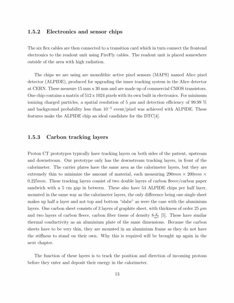
2.4 The final design fully assembled, complete with bolts/rods for attaching to
the calorimeter and side plates. The left side plate has an opening for moving
the conversion layers in and out. . . . . . . . . . . . . . . . . . . . . . . . . . 22
2.5 One of the carbon sheets which will be used as a sensor chip carrier for the
tracking layers. Thickness: 225 µm. . . . . . . . . . . . . . . . . . . . . . . . 25
2.6 pCT design by A. van den Brink, Utrecht University. Tracking layers mounted
onto the calorimeter support structure by the green rods, circled in red,
through holes in the aluminium spacers. The layers are kept in their posi-
tions by nuts on the rods. . . . . . . . . . . . . . . . . . . . . . . . . . . . . 26
vi
2.7 Simple mechanical support seen from the front. . . . . . . . . . . . . . . . . 27
2.8 My mechanical support design, with holes for attaching to the calorimeter . 28
3.1 Standard air vents which connects to a round air supply tube . . . . . . . . 30
3.2 pCT base plate with vents and support pillars, all of which sits below the
calorimeter . . . . . . . . . . . . . . . . . . . . . . . . . . . . . . . . . . . . 31
3.3 Two early attempts at designing the end pieces for the tracking layer air
cooling. A: One big slit covers both tracking layers with one stream of air. B:
four slits which directs the air towards each side of both layers . . . . . . . . 32
3.4 First air cooling design attached to the main vent at the bottom of the
calorimeter, circumfering the support pillar . . . . . . . . . . . . . . . . . . . 33
3.5 The second air cooling design . . . . . . . . . . . . . . . . . . . . . . . . . . 34
3.6 The third and final air cooling design and how they attach to the main vent 34
3.7 The final design with carbon plates . . . . . . . . . . . . . . . . . . . . . . . 35
3.8 Final air cooling design for tracking layers . . . . . . . . . . . . . . . . . . . 36
3.9 Test setup for cooling of the tracking layers . . . . . . . . . . . . . . . . . . . 37
4.1 Illustrating free and forced air cooling convection in a double carbon tracking
layer . . . . . . . . . . . . . . . . . . . . . . . . . . . . . . . . . . . . . . . . 44
4.2 The temperature difference, Tdiff in a carbon sheet of different thicknesses
Ly, as a function of the thermal conductivity k . . . . . . . . . . . . . . . . . 51
4.3 Sheet thickness Ly as a function of the temperature difference, plotted for
different values of the thermal conductivity k . . . . . . . . . . . . . . . . . . 52
4.4 Illustration of different areas of the thermal resistance calculations and axis
of symmetry for said calculations . . . . . . . . . . . . . . . . . . . . . . . . 53
4.5 The temperature difference in the carbon carrier sheet as a function of air
speed, with conduction from water cooling, free convection and forced con-
vection from air cooling . . . . . . . . . . . . . . . . . . . . . . . . . . . . . . 57
4.6 An example of how the Workbench interface looks in ANSYS student version 60
4.7 An example of how the setup for the first set of steady-state simulations look 62
4.8 Steady-state simulation of temperature of the carbon carrier plate with water
cooling and heat load distributed over the whole plate . . . . . . . . . . . . . 62
4.9 Comparison of the calculated values to the simulations using the carbon track-
ing model for the pCT . . . . . . . . . . . . . . . . . . . . . . . . . . . . . . 64
vii
4.10 Comparison of the calculated values to the simulations using the cooling test
model made in Utrecht . . . . . . . . . . . . . . . . . . . . . . . . . . . . . . 65
4.11 An example of how the setup for the fluid simulations look . . . . . . . . . . 67
4.12 Temperature contour of the fluid-solid interface of the carrier plate for only
convection on the pCT carbon sheet model . . . . . . . . . . . . . . . . . . . 68
4.13 Comparison of the calculated values to the Fluent fluid simulations . . . . . 69
5.1 . . . . . . . . . . . . . . . . . . . . . . . . . . . . . . . . . . . . . . . . . . . 74
5.2 . . . . . . . . . . . . . . . . . . . . . . . . . . . . . . . . . . . . . . . . . . . 75
5.3 Air speed measurements above the outlet . . . . . . . . . . . . . . . . . . . . 76
5.4 Measured air speed along the slit (z-direction), 1.5 cm above the outlet. Mea-
sure for four different voltages on the fan . . . . . . . . . . . . . . . . . . . . 77
5.5 . . . . . . . . . . . . . . . . . . . . . . . . . . . . . . . . . . . . . . . . . . . 78
5.6 Example of table of measured temperatures [°C] from the air cooling experiment. 80
5.7 Measured temperature of aluminium plate and temperature difference from
ambient temperature, averaged over five different positions. . . . . . . . . . . 81
5.8 Results from calculations for only convection, power generation corresponding
to heating tape experiment . . . . . . . . . . . . . . . . . . . . . . . . . . . . 84
5.9 Results from calculations with convection including contribution from radiation 84
5.10 Results from calculations including a tentative constant resistance accounting
for all unknown thermal resistance . . . . . . . . . . . . . . . . . . . . . . . 85
5.11 Measured temperature difference for the heat loads corresponding to the cal-
culations of this section. . . . . . . . . . . . . . . . . . . . . . . . . . . . . . 86
5.12 Example of steady state simulation solution, for 4.13W heat load and convec-
tion coefficient h=17.6 . . . . . . . . . . . . . . . . . . . . . . . . . . . . . . 87
5.13 Results from steady state thermal simulation for the experimental setup model 88
5.14 Results from fluid air flow simulation for the experimental setup model . . . 89
viii

List of Tables
4.1 Results from thermal resistance calculations. Contribution from
each cooling effect, their reciprocals and the running total resistance. 56
4.2 Results for ∆T . . . . . . . . . . . . . . . . . . . . . . . . . . . . . . . . . 56
4.3 Comparison of calculated values to simulation results . . . . . . . . . 63
ix

Chapter 1
Introduction
The Bergen pCT collaboration was established to design and build a new prototype proton
CT scanner, used as both tracking and energy/range detector. This is an improvement on
previous designs, using a new type of pixel detector chip developed at CERN which made
this feature posible. My work on this project has been focused on the mechanical properties
of the tracking layers, i.e. the design of the mechanical support and the thermal properties
with regard to heating of the chips and mechanisms for cooling.
Since proton CT is developed to be used in cancer treatment, there will be an introduction
about what kind of diseases cancer is, the basic biology of cancer and some key numbers
from the latest statistics, which show why this is one of the big subjects in the development
of new medical technology. My work is a part of a bigger project that can greatly benefit
the field of cancer treatment in the future but to get a sense of why that is, it is important
to understand how these diseases work and how they are treated.
1.1 Cancer
Cancer is a group of diseases involving abnormal cell growth with the potential to invade
or spread to other parts of the body. These contrast with benign tumors, which do not
spread. Cancer is an umbrella term that includes about 200 different diseases. These can
be quite different, but they all have in common some kind of uncontrolled cell division. In
1

most cases, changes in cell division activity are due to mutations in the genes that encode
cell cycle regulator proteins. These mutations can be the result of any number of known
and unknown reasons. The mutated cancer cells differ from healthy cells in ways that make
them divide uncontrollably, bypassing the mechanisms that usually make cells stop dividing.
Cancer cells are also able to expand into surrounding tissue (invasion) or migrate to other
parts of the body through a process called metastasis, making the disease particularly hard
to keep track of and treat properly.
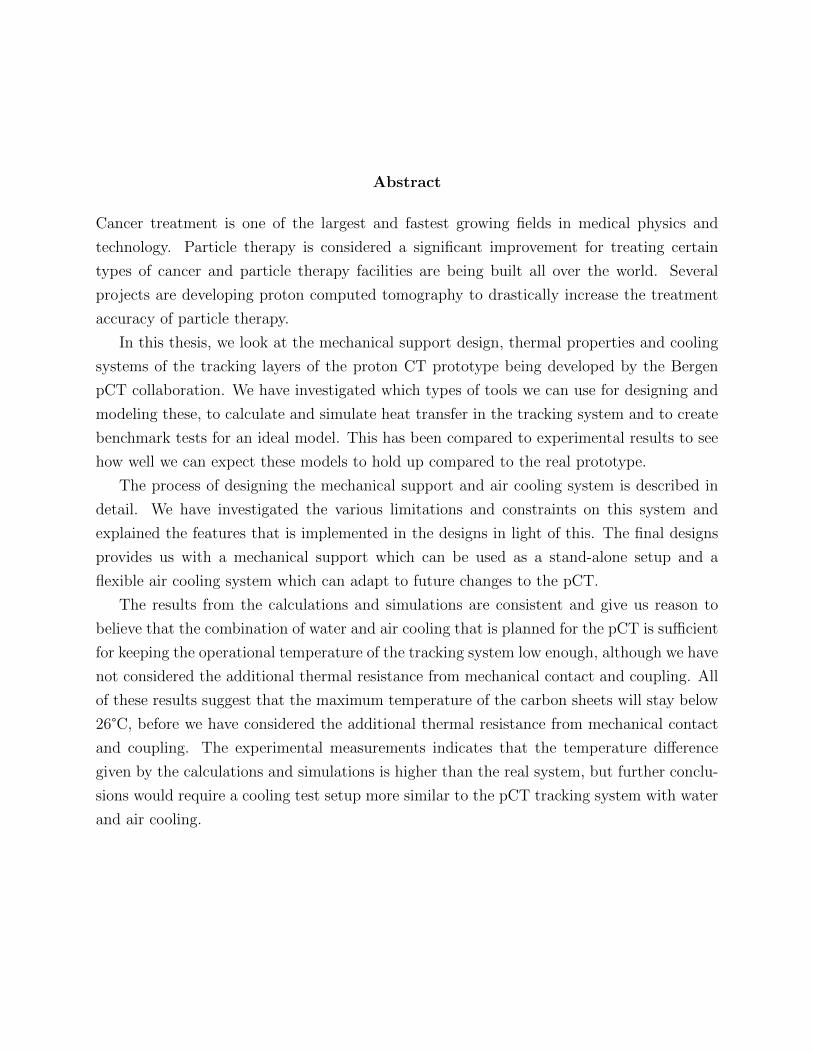
Cancer is one of the leading causes of death in the developed world today. In Norway,
there were 34 979 new cancer cases reported in 2019. 11 049 people died of cancer and by
the end of the year, 294 855 people were alive after having had at least one cancer diagnosis
at some point, according to the newest data available [10]. Even though these diseases kill
a lot of people each year, their mortality rates keep declining as advances in medicine and
technology are made (see fig 1.1). There are several different treatment modalities for cancer,
chemotherapy, immunotherapy, surgery and radiation therapy, the last of which is the main
focus in medical physics.
2
Figure 1.1: Age-standardized(Norwegian standard) mortality rates per 100 000 person-yearsfor selected cancers [10]
Source:Cancer in Norway 2019
1.2 Radiation Treatment
Classical radiation therapy as cancer treatment is using high intensity x-rays, usually pro-
duced with a linear particle accelerator (linac). The linac works the same way as an x-ray
tube, where electrons are accelerated from a cathode to an anode, hitting a target with a
high atomic number, e.g. tungsten, to produce photons. What makes it different is the mid-
dle part where electrons are accelerated from about 50 keV up to several MeV, producing
ionizing radiation with much higher energy than what is required for imaging. This ionizing
radiation is used to damage or destroy cancer cells.
3

The photon beam has its highest dose deposition a few centimeters after entering the
tissure as one can see from the dose distribution graph below (figure 1.2). Also, we know
that there is a correlation between ionizing radiation to healthy tissue and the development
of a new cancer later on. This leads us to the question regarding treatment planning, how
one would deliver the required dose to the target while minimizing the dose delivered to
healthy tissue.
Figure 1.2: Depth dose curves for different types of radiation treatment [1]
Source: https://www.researchgate.net
The optimization of dose distribution, giving as much dose as prescribed to the tumor and
as little as possible to healthy tissue, is achieved through computer simulation of the treat-
ment plans. The dose planning software is a very intuitive interface for medical physicists.
After importing CT images of a patient, one can program the linac by simple parameters
like beam energy, movement of the gantry (linac head) to get complicated intensity mod-
ulated radiotherapy (IMRT) programs. The dose plan is then used by the linac to control
4
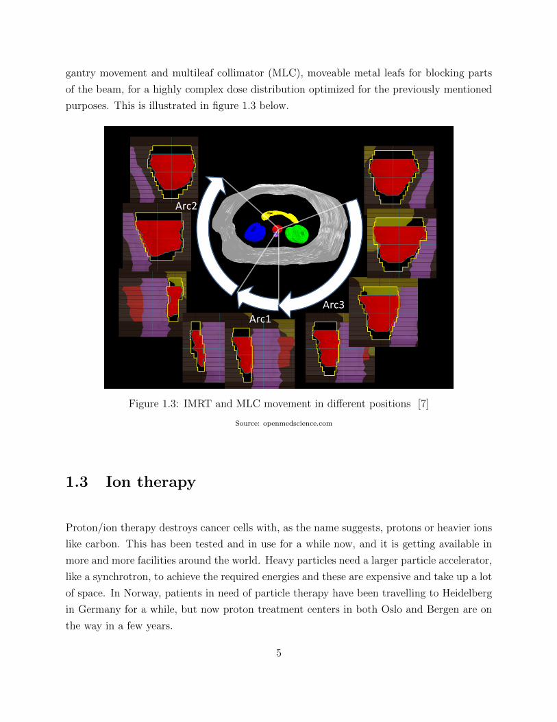
gantry movement and multileaf collimator (MLC), moveable metal leafs for blocking parts
of the beam, for a highly complex dose distribution optimized for the previously mentioned
purposes. This is illustrated in figure 1.3 below.
Figure 1.3: IMRT and MLC movement in different positions [7]
Source: openmedscience.com
1.3 Ion therapy
Proton/ion therapy destroys cancer cells with, as the name suggests, protons or heavier ions
like carbon. This has been tested and in use for a while now, and it is getting available in
more and more facilities around the world. Heavy particles need a larger particle accelerator,
like a synchrotron, to achieve the required energies and these are expensive and take up a lot
of space. In Norway, patients in need of particle therapy have been travelling to Heidelberg
in Germany for a while, but now proton treatment centers in both Oslo and Bergen are on
the way in a few years.
5
As of July 2020 there are 104 operating particle therapy facilities world wide, according
to the Particle Therapy Co-Operative Group [6].Advances and improvements concerning this
type of cancer treatment is worked on by physicists and engineers all over the world, since
this is one of the best options to treat many types of cancer. Because of the promising
results from this kind of treatment, there are more facilities planned and currently under
construction.
Due to the high accuracy of the dose delivery and there being a lot less radiation to
surrounding tissue, the results of treating cancer situated deep inside the body and/or near
organs at risk can be much better with proton/ion therapy than with traditional radiother-
apy. Protons and ions lose some of its energy along the way but after a set distance (decided
by the energy of the beam) and the rest of the energy is deposited locally. This means we get
almost the entire dose delivered at this given distance (figure 1.2), and this in turn makes it
a lot easier to reduce the dose to surrounding tissue drastically. The total doses delivered to
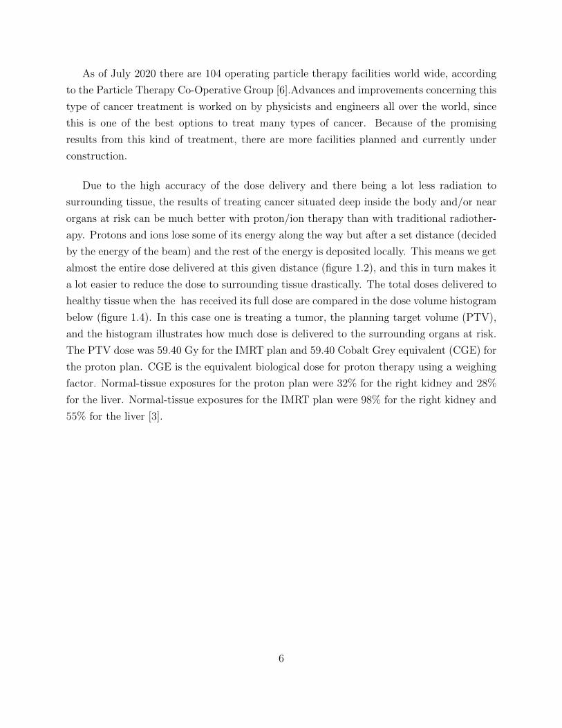
healthy tissue when the has received its full dose are compared in the dose volume histogram
below (figure 1.4). In this case one is treating a tumor, the planning target volume (PTV),
and the histogram illustrates how much dose is delivered to the surrounding organs at risk.
The PTV dose was 59.40 Gy for the IMRT plan and 59.40 Cobalt Grey equivalent (CGE) for
the proton plan. CGE is the equivalent biological dose for proton therapy using a weighing
factor. Normal-tissue exposures for the proton plan were 32% for the right kidney and 28%
for the liver. Normal-tissue exposures for the IMRT plan were 98% for the right kidney and
55% for the liver [3].
6

Figure 1.4: Dose-volume histogram (DVH) data for a proton plan (delivered) and corre-sponding optimized intensity-modulated radiotherapy (IMRT) plan.
Source: researhgate.net
The peak of the depth dose curve is called the Bragg peak, and is located at the depth
where the particle stops and deposits its energy. The location of the Bragg peak is depend-
ing on the energy of the particle and the stopping power of the material that the particle
passes through. Due to this dose distribution, accuracy becomes important in this type of
cancer treatment. Without a way to deliver the dose with sub-mm precision, one would risk
delivering a quite large dose to the healthy tissue surrounding the target, and in turn would
destroy the entire case for a better dose distribution than photon treatment.
One of the main challenges with accuracy in particle therapy is the imaging modalities
available for creating a treatment plan. X-ray computed tomography (CT) is the go-to
for mapping the stopping power in tissue when planning dose delivery because of the good
resolution and contrast one can achieve in three-dimensional pictures of a patient. For
7

classical radiotherapy this is working well because the photon absorption that is mapped in
the CT image is the same as for the radiation used in the treatment, for photons that is,
thus it translates directly from plan to treatment.
Also, because the dose distribution for photons is quite “spread out” to begin with, the
range uncertainty for the dose plan is not dependent on sub-millimeter precision. With ion
radiation treatment on the other hand, a small difference in the position of the Bragg peak
could result in a huge difference in dose delivered to healthy tissue or organs. Because of
the stopping power depending on other factors for ions than photons, the necessary stopping
power conversion results in errors up to 3.5%, corresponding to up to 4 mm of possible
misplacement of the Bragg peak at 10 cm water equivalent range in the patient [4].
Another thing to consider with the accuracy of particle therapy is range straggling. Due
to the statistical nature of the energy loss process, there is a small variation in the depth of
the end point of each ion. A mono-energetic proton beam will therefore have an extended
Bragg peak area compared to a single proton [9].
1.4 Proton Computed Tomography
As explained in the previous section, the location of the Bragg peak, i.e. where the particle
deposits a large fraction of its energy, is determined by the particle’s initial energy. For
particle therapy this would be somewhere inside the patient’s body. If we use significantly
higher energies, the Bragg peak will be somewhere on the other side of the patient (figure
1.5) and if we can detect the particle’s residual energy, we can use this to reconstruct an
image. This would produce a two dimensional image, so by rotating the beam and detector,
we would be able to reconstruct a 3D image of the body, just like a regular x-ray CT.
Most proton computed tomography (pCT) prototypes are constructed with tracking lay-
ers and a detector. The tracking layers are important for reconstructing the path of the
individual particles. It is common to have tracking layers upstream of the beam, on the
opposite side of the patient from the detector, but the one we will be looking at only has
tracking layers downstream like in figure 1.5. After passing the tracking layers, which we
will come back to as they are the main subject of my thesis, we have a detector. This is
8
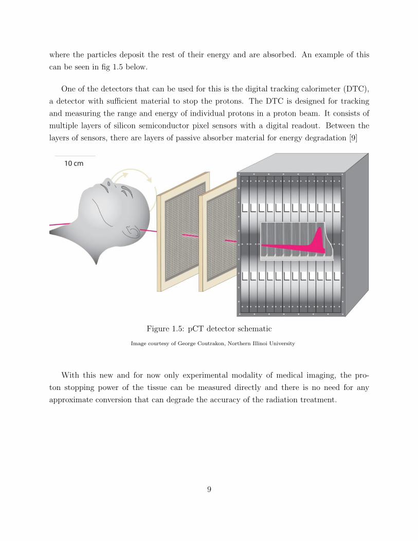
where the particles deposit the rest of their energy and are absorbed. An example of this
can be seen in fig 1.5 below.
One of the detectors that can be used for this is the digital tracking calorimeter (DTC),
a detector with sufficient material to stop the protons. The DTC is designed for tracking
and measuring the range and energy of individual protons in a proton beam. It consists of
multiple layers of silicon semiconductor pixel sensors with a digital readout. Between the
layers of sensors, there are layers of passive absorber material for energy degradation [9]
Figure 1.5: pCT detector schematic
Image courtesy of George Coutrakon, Northern Illinoi University
With this new and for now only experimental modality of medical imaging, the pro-
ton stopping power of the tissue can be measured directly and there is no need for any
approximate conversion that can degrade the accuracy of the radiation treatment.
9

1.5 Bergen pCT prototype
Figure 1.6: The general structure of the Bergen pCT system
Bergen pCT collaboration
In my work on this thesis, I have been a part of the Bergen pCT group, an international
collaboration of physicists and engineers working on making a new version of the proton CT
scanner.
The most distinctive feature of the prototype design is the employment of a digital
tracking calorimeter (DTC), which can be seen in figure 1.6 as the main part with the
41 layers. Previously, a calorimeter with such features was built and successfully tested
with particle beams showing very good performances despite a number of imperfections,
most notably a large fraction of dead or otherwise unusable pixels. The Bergen pCT is an
evolution of the described prototype: a novel DTC specifically designed and optimized for
pCT, used as both tracking and energy/range detector [4]. This improvement is thanks to a
new chip for particle detection called ALPIDE.
10
1.5.1 Calorimeter layers
The prototype currently being made by the Bergen pCT group is a 41 layer calorimeter
detector. Each layer consists of a 1.5 mm aluminium absorber plate situated between two
aluminium carrier plates of 1 mm thickness for a total 3.5 mm of aluminium per layer. The
carrier plate is made up from a top and bottom “slab”, each 290 mm wide and 100 mm in
height. On the carrier plates, we glue flex cables with 9 sensor chips each, called a “string”,
three strings per slab. The top and bottom slabs make up one half layer for a total 54
sensors, covering approximately half the plate (see fig 1.7 of carrier plate below).
The second half layer is placed on the opposite side of the absorber plate, with the flex
cables pointing in the other direction. This makes it possible to fit all the cables and readout
electronics in the detector. The sensors on this half layer are positioned parallel to where the
flex cables of the first layer are, making the whole area in one full layer covered by sensors.
11

Figure 1.7: (A)Half a layer consisting of a top slab and a bottom slab. Each of the slabs isbuilt by gluing three strings of ALPIDE sensors to a aluminium carrier. (B) Schematic sideview of two layers in the calorimeter (left), and half a layer with details (right) [4]
.
12
1.5.2 Electronics and sensor chips
The six flex cables are then connected to a transition card which in turn connect the frontend
electronics to the readout unit using FireFly cables. The readout unit is placed somewhere
outside of the area with high radiation.
The chips we are using are monolithic active pixel sensors (MAPS) named Alice pixel
detector (ALPIDE), produced for upgrading the inner tracking system in the Alice detector
at CERN. These measure 15 mm x 30 mm and are made up of commercial CMOS transistors.
One chip contains a matrix of 512 x 1024 pixels with its own built in electronics. For minimum
ionizing charged particles, a spatial resolution of 5 µm and detection efficiency of 99.99 %
and background probability less than 10−5 event/pixel was achieved with ALPIDE. These
features make the ALPIDE chip an ideal candidate for the DTC[4].
1.5.3 Carbon tracking layers
Proton CT prototypes typically have tracking layers on both sides of the patient, upstream
and downstream. Our prototype only has the downstream tracking layers, in front of the
calorimeter. The carrier plates have the same area as the calorimeter layers, but they are
extremely thin to minimize the amount of material, each measuring 290mm × 200mm ×0.225mm. These tracking layers consist of two double layers of carbon fleece/carbon paper
sandwich with a 5 cm gap in between. These also have 54 ALPIDE chips per half layer,
mounted in the same way as the calorimeter layers, the only difference being one single sheet
makes up half a layer and not top and bottom “slabs” as were the case with the aluminium
layers. One carbon sheet consists of 3 layers of graphite sheet, with thickness of order 25 µm
and two layers of carbon fleece, carbon fiber tissue of density 8 gm2 [5]. These have similar
thermal conductivity as an aluminium plate of the same dimensions. Because the carbon
sheets have to be very thin, they are mounted in an aluminium frame as they do not have
the stiffness to stand on their own. Why this is required will be brought up again in the
next chapter.
The function of these layers is to track the position and direction of incoming protons
before they enter and deposit their energy in the calorimeter.
13

The fact that the carbon sheets are so thin also makes them very fragile and vulnerable.
The same goes for the other parts of the tracking layers, that is the ALPIDE chips and the
flex cables they are mounted on. This will be considered in the following chapters as one of
our main considerations, especially in the design of the mechanical support and air cooling.
This part of the proton CT, the carbon tracking layers, is the main subject of this thesis.
In the next chapter there will be a description of how the mechanical support for the layers
have been designed, both as mounted in front of the calorimeter in the detector and as
a stand-alone experimental setup for beam tests. This will be presented as solutions to
different potential challenges we might face in the future and will introduce features that
might be useful for testing, calibration, research and clinical use of the proton CT.
14

Chapter 2
Mechanical support for the carbon
tracking layer
I have been concerned with the mechanical properties, design and cooling of the tracking
layers in front of the calorimeter. Therefore, only the thermal and mechanical aspect will be
the subject of this thesis. More details about things like Monte Carlo simulation, electronics
and programming can be found in the other theses and papers published by the Bergen pCT
group, some of which are cited here.
The tracking layers should be mounted in front of the calorimeter in some way, and
we would also need a stand-alone test rig for the tracking layers when they are assembled
and ready. Since the mechanical setup for the calorimeter part, transition cards and readout
system was being developed simultaneously, by different teams in the project, the constraints
were changing and the design needed to be updated. Here I report how my design changed
over time with changing design constraints.
The designs of the mechanical support and of the air cooling system in chapter 3 are
all made using the computer aided design (CAD) software CREO Parametric. After this
overview of the design process has been presented, I will explain the different functions and
the purpose they serve more in depth.
15

2.1 Limitations, constraints and trade-offs
Before getting into the description of the design itself, we must address the potential chal-
lenges we will have to face regarding the mechanical properties of the detector. When we
eventually take our design from the drawing board into the real world, one would like to
have considered as much of this as possible. This process makes up the foundation for the
decisions I have made and is therefore at least as important as the design itself. Even though
the final prototype is not ready, I have tried to think as far ahead as possible and consider
every aspect from early testing to clinical use. I should also mention that not all of the
challenges I bring up here are directly addressed in my design, and that the solution to some
of them are still open-ended questions.
2.1.1 Amount of material in front of detector
The tracking layers are the first layers of the detector that are hit by the incoming protons.
To make the particle tracking, and in turn the path reconstruction, as precise as possible
we would like to have as little scattering as possible. This would imply that we try to keep
the amount of material in front of this first layer to a minimum, which is the reason why we
have chosen the thin carbon sheets for the tracking layers, to minimize scattering.
To implement a few things that we thought could be useful, we may have opened up for
more scattering from the support structure. Especially to make a mechanical support that
can be used as a stand-alone tracking layer setup.
2.1.2 Mechanical stability and physical protection
In the early stages, testing will be in relatively controlled environments. This means, with
regards to mechanical stability, we do not have to be too worried about our setup. The
structure will be standing still during tests and will be used only by people associated with
the project, that knows how fragile it is and how it should be handled.
16

At some point, we might see our detector in quite different circumstances, that is, inside
a moving gantry, in a clinical setting with patients and hospital workers. In this case, there
are a few things that may become more important.
Stability in x-, y- and z-direction: if there is any chance that the tracking layer structure
experiences any external forces, this stress and strain should be expected and accounted
for. On the one hand gravity, if the layers are not fixed in all three directions, can be an
issue if the support is attached to a moving structure. On the other hand, more transient
forces like someone pushing it (be that on purpose or by accident) could damage or destroy
something even though the structure is fixed in all directions. We should at least be certain
that these scenarios would not destroy the tracking layers or cause big problems like the
need to recalibrate the software.
Physical protection overlaps to some extent with the challenges regarding stability. In
a clinical environment, something might easily poke a hole through a 0.2 mm thick carbon
sheet. How to physically protect the front end of the detector without being a huge disad-
vantage with regards to scattering is a potential challenge down the line. This was taken
into consideration for the first design but for the later ones, the focus has been on more
immediate concerns like implementation of air cooling and conversion layers, all of which
I will get back to. The physical protection will be addressed at a later point, when this
becomes more important.
2.1.3 Weight and complexity
Another restriction regarding the amount of material is the total weight of the support
structure. All the parts are made from Aluminium, and with the final design the weight of
the frame alone is 1.42 kg. It is in no way a minimalist approach to a support structure for
the tracking layers, there is a conscious choice to make a robust mechanical support, as this
is one of the main trade-offs in the design in this part of the detector. This overlaps a lot
with the other limitations.
This design is an idealized model that would need some refining if it were to be produced
but it would be a very good test module for the tracking layers that takes into consideration
a lot of the things that I will discuss in the rest of this chapter. This justifies the design
complexity. Some of the limitations discussed in this section will be revisited later in this
chapter for further discussion.
17
2.1.4 Plastic and tungsten foil - conversion layers
We want to have conversion materials between the two tracking layers, to be able to detect
neutrons and photons. In short, the particles detected by the second tracking layer that
were not detected by the first, are the particles converted by the layer in between.
The mechanical support of the tracking layers is not just supposed to hold two thin layers
of carbon, but also two layers of different materials. A slab of plastic of 1-2 cm thickness,
polymethylmethacrylate (PMMA) for example, and a sheet of some element with a high
atomic number, in our case tungsten foil, would be inserted between the tracking layers.
These each have a specific function of converting particles into charged that the ALPIDEs
can detect.
The PMMA layer converts fast neutrons to fast protons, to be detected by the ALPIDE
chips. This way we can detect the amount of neutrons passing through a phantom or patient
as a result of our proton beam, before and after the plastic layer.
The tungsten foil converts photons to electrons or positrons, so that the amount of
photons can be passively detected by the calorimeter.
2.2 The mechanical support design
This section is describing the design process, my ideas and the motivation behind each step.
I will go through the different design ideas and I will evaluate my choices for each feature of
the final result, in light of the constraints and limitations that have been presented, in the
next section.
18

2.2.1 First design ideas
Figure 2.1: The first mechanical support design, with nine identical slots for the trackingand convection layers
.
This was the first suggestion as a mechanical support. The idea was making two identical
plates like this, one on top and one at the bottom. It covers the whole width of the calorimeter
and is bolted onto the front of the calorimeter through the four holes. This way, the two
plates are just suspended in the air and the tracking layer frames would be part of the
mechanical structure. There are nine slots for inserting the layers with variable distance and
in any order. The rectangular hole in front is to insert a protective sheet.
This first design is quite simple but a lot of the same ideas are developed further in the
next design.
19

(a) Empty frame (b) Assembled
Figure 2.2: Pictures of the second design, empty and fully assembled with tracking layerswith water cooling pipes and conversion layers(blue and yellow) in between
The first design was simple and had some flaws, as well as some features that were not
needed at this point. It was not mechanically stable on its own or possible to assemble
independently from the calorimeter. Also, the water cooling pipes on the tracking layer
frames would not fit with this design. The additional slots and the protective sheet are not
needed at this point.
These are the features of the second design:
• Two identical plates(top and bottom) with two grooves for the carbon layers and two
for the scintillator plastic and tungsten foil to slide in from the side. Four cylinders,
one in each corner of the plates is used to hold the structure together.
• The assembly is pretty simple, carbon layers with frames are clamped in place between
the two plates. Once the top and bottom plates have been fastened to the cylinders,
the carbon layers cannot move due to the water cooling pipes on each side. The plastic
and tungsten can slide in and out after assembly.
20

2.2.2 Final design
(a) Empty frame (b) With tracking and conversion layers
Figure 2.3: Pictures of the third and final design
Two possible ways to attach the tracker to the calorimeter:
• Holes in the top and bottom plate for bolts to attach the whole support structure to
the calorimeter, like in the first design.
• Two thinner bolts on each side are attached directly to holes in the spacer of the carbon
layers.
21
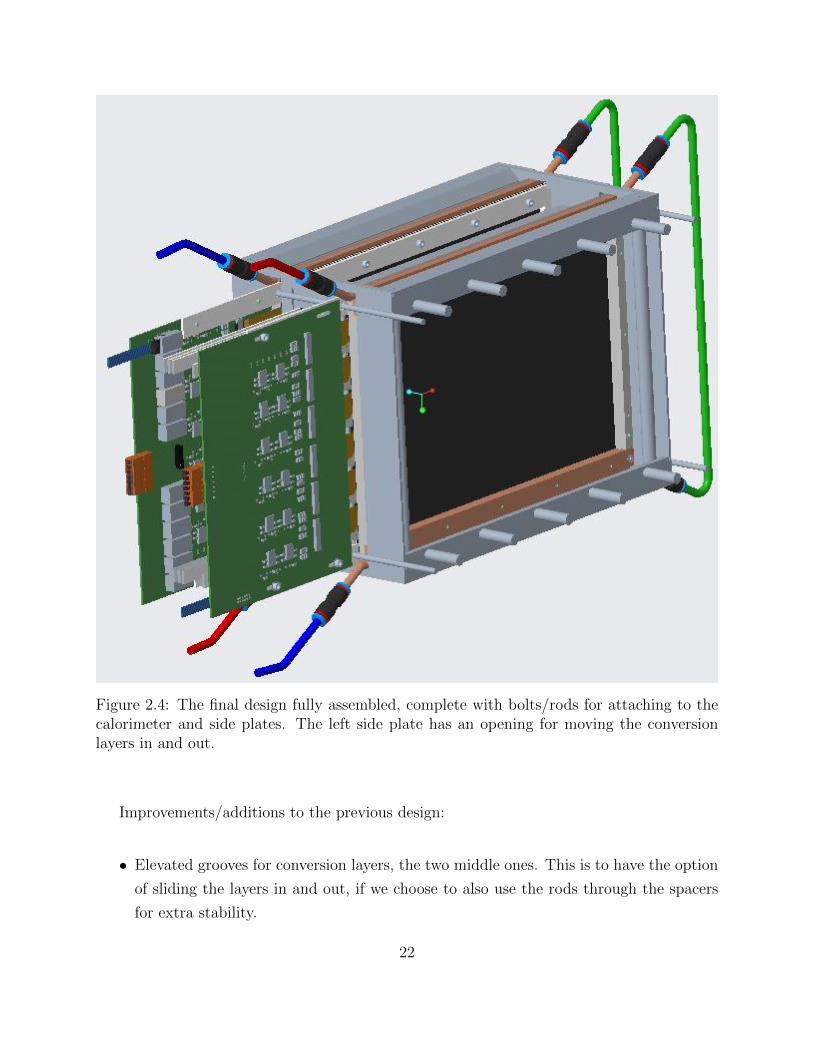
Figure 2.4: The final design fully assembled, complete with bolts/rods for attaching to thecalorimeter and side plates. The left side plate has an opening for moving the conversionlayers in and out.
Improvements/additions to the previous design:
• Elevated grooves for conversion layers, the two middle ones. This is to have the option
of sliding the layers in and out, if we choose to also use the rods through the spacers
for extra stability.
22
• Openings/slits in both plates, above and below the carbon layers, allows for imple-
mentation of air cooling. The idea is to have moderate airflow on each side of each
layer for heat convection, to contribute to keeping the ALPIDE chips within optimal
operational temperature.
• Added plates at each side, to enclose the whole structure. Everything should be fixed
and mechanically stable in every direction, except for the plastic and tungsten layers
sliding out one of the sides. This would have to be fastened with a hinge or something
similar. These plates should also keep the air from the cooling flowing through the
support structure and not escaping out the sides, resulting in loss of cooling effect.
Figure 2.4 displays is the final design fully assembled. At this point there was no more
features to implement in the design and no reason to complicate things further. I will
now discuss the implemented features more in-depth in the next section before drawing a
few conclusions regarding its potential use and comparing this to an alternative mechanical
support design.
2.3 Features of the design and their implementations
based on future needs in research and clinic
2.3.1 Stability
In the x-direction (vertically) this should be very stable. The four pillars joining the top
and bottom plate in each corner are very stable. In the y- and z-direction it would be
stable for all intended use of the detector or as a beam test setup. With enough force, the
top and bottom plates could probably be shifted relative to each other. This is unless the
structure is bolted onto something, e.g. the calorimeter, as was intended in the final design.
In hindsight, it seems like this design might not be the best for this purpose and that it is
better as a stand-alone support. This will be discussed in the next section. In that case, the
stability and how much force will be applied to the structure will have to be evaluated for
the intended use.
23

2.3.2 Modularity
The idea for mounting the plastic layer, the tungsten foil and the two carbon tracking layers
was to make the design as modular as possible, with easy access for inserting/removing
the conversion layers when needed. The first design has 9 grooves for these layers, all the
same size. This way, all the layers could be placed in whichever order we want at different
distances. At this point, the distances between the tracking layers and the placement of
the plastic and Tungsten layers were not decided, and as such the mechanical support was
designed so that they could be moved around. Also, the tracking layers did not have their
cooling pipes, which means they were able to slide in and out. This design was made to keep
all options available.
When the simulation team had decided that 5 cm between the carbon layers was ideal
for tracking, the next design had the position of the tracking layers fixed. The thick slab
of plastic and the thin tungsten foil also had designated slots of corresponding thicknesses
between the tracking layers. The most important thing is that the conversion layers can be
inserted and removed at any time, and this is a feature of the final design as well.
2.3.3 Implementation of air cooling
In investigating the cooling of the carbon sheets, which will be explained in greater detail
in chapter 4, we discovered the limits of the effect of water cooling on the carbon sheets.
In short, the thermal conductivity of the carbon tracking layers that are available for the
prototype makes it so that the water cooling pipes are not sufficient to carry away the heat
produced by the ALPIDE chips in a worst case scenario. We have to make sure to keep the
heating of the chips to a minimum, and with the calculated temperature difference in the
tracking layers being too high, air cooling will be implemented as well. In the final design,
the top and bottom plates in the support structure are opened up for air to flow through on
each side of the carbon layers.
The design of the air cooling system will be discussed in the next chapter.
24

2.3.4 Protecting the tracking layers in a clinical situation
As mentioned earlier, physical protection of the tracking layers, i.e. the front of the detector
can become necessary. The carbon sheets, which is shown in figure 2.5, are very fragile and
shielding them physically could be necessary already at the stage of testing the prototype,
but especially in a clinical setting with patients around and other things outside of our
control.
The simplest version of this would be a metal sheet that covers the front of the first
tracking layer, that would be removed before use. For the time being, i have not included
this in the design but it would be quite simple to make. Eventually, this cover would ideally
be automated and an integrated part of the detector, but that is not necessary for the
purpose of our prototype.
Figure 2.5: One of the carbon sheets which will be used as a sensor chip carrier for thetracking layers. Thickness: 225 µm.
Image by A. van der Brink
25

2.4 Comparing the two mechanical support designs for
the tracking layers
In addition to the design i made, we have a simpler setup for the tracking layers which is a
part of the pCT model made by A. van den Brink at Utrecht University, where the layers
are supported by thin rods attached to the calorimeter (see figures 2.6 and 2.7 below). This
has the absolute minimum of material needed to keep the tracking layers in place.
Figure 2.6: pCT design by A. van den Brink, Utrecht University. Tracking layers mountedonto the calorimeter support structure by the green rods, circled in red, through holes in thealuminium spacers. The layers are kept in their positions by nuts on the rods.
26
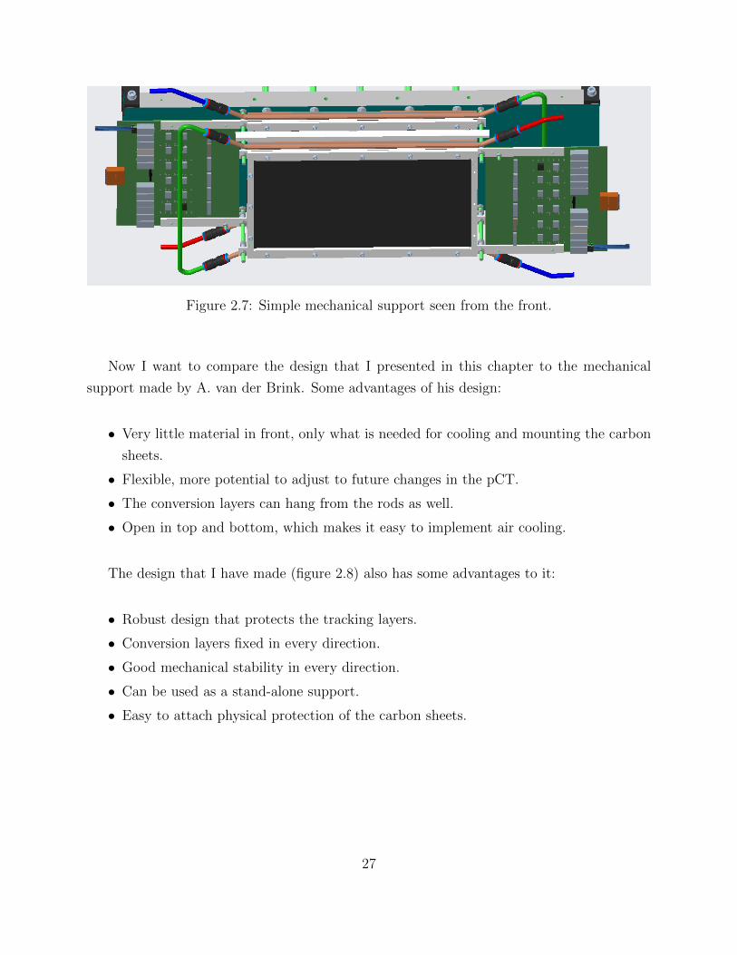
Figure 2.7: Simple mechanical support seen from the front.
Now I want to compare the design that I presented in this chapter to the mechanical
support made by A. van der Brink. Some advantages of his design:
• Very little material in front, only what is needed for cooling and mounting the carbon
sheets.
• Flexible, more potential to adjust to future changes in the pCT.
• The conversion layers can hang from the rods as well.
• Open in top and bottom, which makes it easy to implement air cooling.
The design that I have made (figure 2.8) also has some advantages to it:
• Robust design that protects the tracking layers.
• Conversion layers fixed in every direction.
• Good mechanical stability in every direction.
• Can be used as a stand-alone support.
• Easy to attach physical protection of the carbon sheets.
27

Figure 2.8: My mechanical support design, with holes for attaching to the calorimeter
With these two designs available to us, it seems like the most flexible solution by van der
Brink will stay in the pCT design and my design will be used for only the tracking layers
as a stand-alone support. This means we can adjust the setup of the tracking layers with
regards to any changes to other parts of the detector. We will keep in mind this flexibility
also in the design of the air cooling of these layers.
28

Chapter 3
Air cooling design
Now we will look at the different attempts to design an air cooling system for the tracking
layers. I will give a short presentation of this work, as it is not as complex a design as for
the support structure. Also, the final design is made by A. van der Brink but my designs
have been a part of this process.
There are two parts to this design process which are overlapping and interdependent of
each other, the tracking layer cooling for the pCT and for the air cooling test setup made
in Utrecht. Geometrically, with regards to the air cooling, the two are very similar so this
design should work for both cases.
3.1 The design task
Most of the air cooling system looks the same for the two different cases. I will explain what
the test setup looks like, but first of all I would like to present the general idea of the air
cooling system as a whole, and what part my design has in it.
The air cooling starts with an air supply or ventilation in the back of the pCT. This is
connected to a round adapter which in turn is connected to a 225mm x 25mm rectangular
vent which is split in four. This can be seen in figure 3.1 below. The rectangular vent then
sits underneath the calorimeter in the pCT. These parts are standard industrial vents which
29
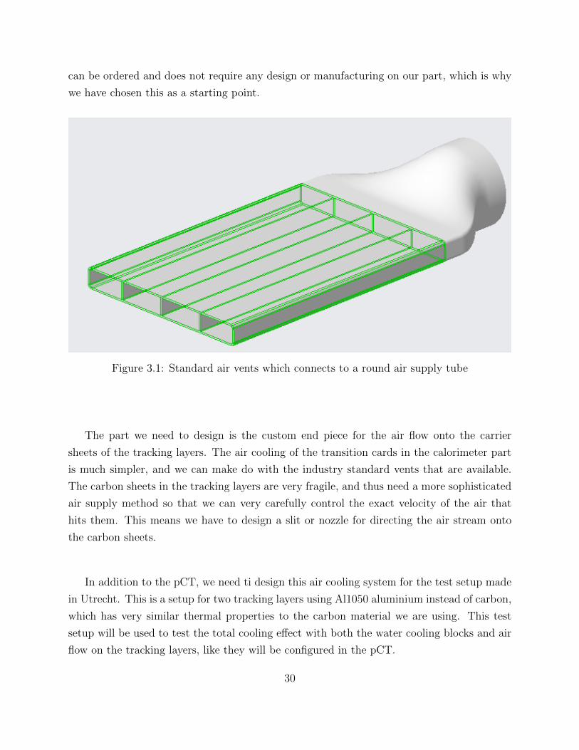
can be ordered and does not require any design or manufacturing on our part, which is why
we have chosen this as a starting point.
Figure 3.1: Standard air vents which connects to a round air supply tube
The part we need to design is the custom end piece for the air flow onto the carrier
sheets of the tracking layers. The air cooling of the transition cards in the calorimeter part
is much simpler, and we can make do with the industry standard vents that are available.
The carbon sheets in the tracking layers are very fragile, and thus need a more sophisticated
air supply method so that we can very carefully control the exact velocity of the air that
hits them. This means we have to design a slit or nozzle for directing the air stream onto
the carbon sheets.
In addition to the pCT, we need ti design this air cooling system for the test setup made
in Utrecht. This is a setup for two tracking layers using Al1050 aluminium instead of carbon,
which has very similar thermal properties to the carbon material we are using. This test
setup will be used to test the total cooling effect with both the water cooling blocks and air
flow on the tracking layers, like they will be configured in the pCT.
30
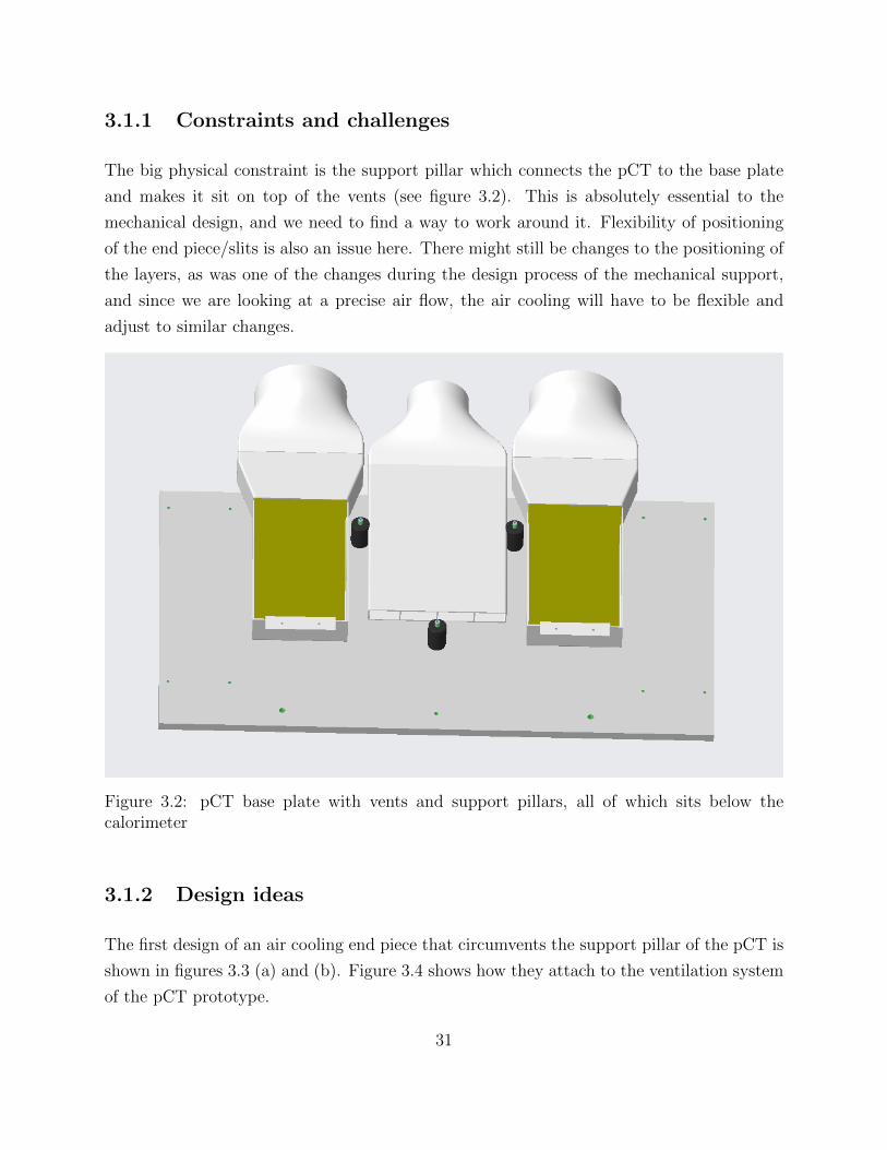
3.1.1 Constraints and challenges
The big physical constraint is the support pillar which connects the pCT to the base plate
and makes it sit on top of the vents (see figure 3.2). This is absolutely essential to the
mechanical design, and we need to find a way to work around it. Flexibility of positioning
of the end piece/slits is also an issue here. There might still be changes to the positioning of
the layers, as was one of the changes during the design process of the mechanical support,
and since we are looking at a precise air flow, the air cooling will have to be flexible and
adjust to similar changes.
Figure 3.2: pCT base plate with vents and support pillars, all of which sits below thecalorimeter
3.1.2 Design ideas
The first design of an air cooling end piece that circumvents the support pillar of the pCT is
shown in figures 3.3 (a) and (b). Figure 3.4 shows how they attach to the ventilation system
of the pCT prototype.
31

(a) Design 1
.
(b) Design 2
.
Figure 3.3: Two early attempts at designing the end pieces for the tracking layer air cooling.A: One big slit covers both tracking layers with one stream of air. B: four slits which directsthe air towards each side of both layers
32
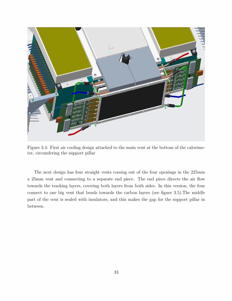
Figure 3.4: First air cooling design attached to the main vent at the bottom of the calorime-ter, circumfering the support pillar
The next design has four straight vents coming out of the four openings in the 225mm
x 25mm vent and connecting to a separate end piece. The end piece directs the air flow
towards the tracking layers, covering both layers from both sides. In this version, the four
connect to one big vent that bends towards the carbon layers (see figure 3.5).The middle
part of the vent is sealed with insulators, and this makes the gap for the support pillar in
between.
33

Figure 3.5: The second air cooling design
The final version is a refinement of the previous design. The four vents and end pieces
are made to extend to the two carbon layers separately, directing the air towards each layer
from below and providing even airflow on both sides of each layer. You can see this design
with and without the carbon layers in figures 3.6 and 3.7.
Figure 3.6: The third and final air cooling design and how they attach to the main vent
34
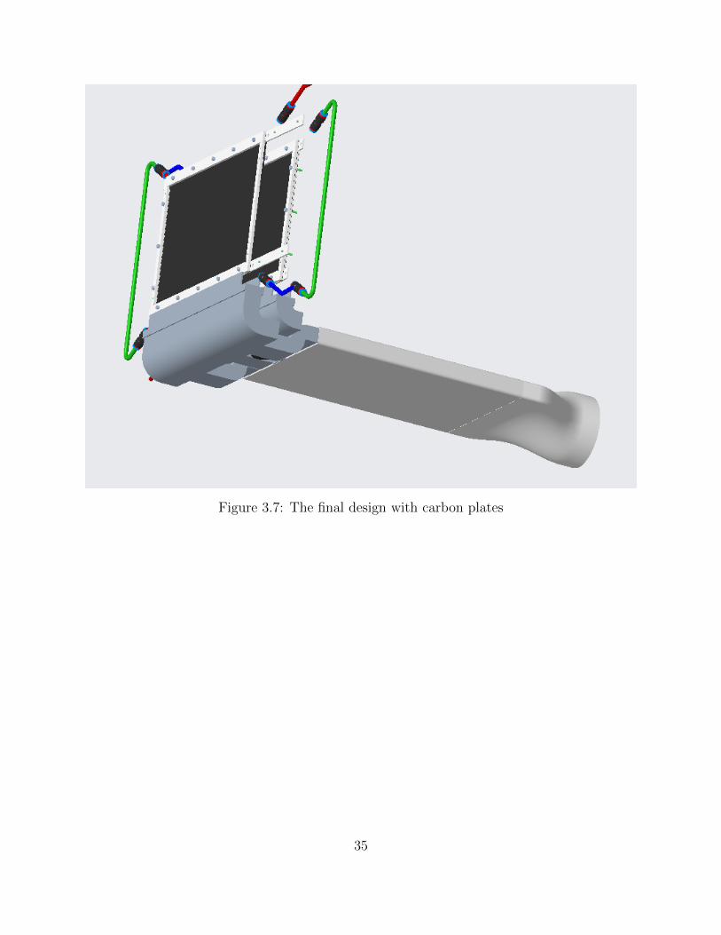
Figure 3.7: The final design with carbon plates
35

3.2 Finalizing the design
This design process was in collaboration with A. van der Brink at Utrecht university, who is
in charge of the design of the pCT. After i completed the design in figure 3.7, van der Brink
finished the design and implemented features that improved the functionality and flexibility
a lot. The result is a box with four slits/nozzles, one for each carrier plate, tilted a bit
towards its corresponding plate. These slits are also movable in the y-direction (front to
back) which makes it flexible in case of changes later in the process. This design can be seen
in figure 3.8.
Figure 3.8: Final air cooling design for tracking layers. Design by A. van der Brink, Utrecht University
The duct that connects to the end piece with the moveable slits is the same for the pCT
and the test setup (figure 3.9). This is because we want to test how the air cooling works
with the exact same conditions, how the airspeed out of the slits relates to the volumetric
air flow from the fan or ventilation and what kind of cooling effect we will see as a result of
this.
36

Figure 3.9: Test setup for cooling of the tracking layers. Design by A. van der Brink, Utrecht University
37

38
Chapter 4
Cooling of carbon sheets - a
theoretical model
The second part of my thesis is regarding the heat transferred into and out of the carbon
carrier sheets of the tracking layers, and to look at the effect of water and air cooling
respectively and combined. In this chapter I will present the theory and empirical formulas
that I have used to model the carbon tracking layer and experimental test setups. The
carbon layers have been described in detail in the previous chapters.
There are two test setups for cooling experiments. One is a small aluminium plate with
a heating tape which I have assembled in Bergen with help from some of the engineers on
the pCT project. The other one is a full scale aluminium model of the tracking layer that
has been assembled in the workshop in Utrecht and are going to be sent to Bergen.
The temperature difference across the carrier plate and how it varies with certain pa-
rameters is the main subject of this section. There are also some other simple calculations
which are mentioned, the air volume flow from our cooling system, the frictional force on
the plates from the air flow, the cooling noise and vibration frequency from the air cooling
supply/fan. This makes a foundation for the reasoning behind some of the choices we have
done in designing and ordering parts for the pCT. This also hopefully gives us a look ahead
at what to expect when tests are run on the prototype. These other subjects are somewhat
outside the scope of my thesis and will not be investigated further.
39

Several parameters goes into these thermal processes, some of which we can control and
some that are inherent in the materials, and it all adds up to a complex thermodynamic
system. We will therefore evaluate these to the extent that we can, given the information
and the techniques available. Some of this will be idealized situations and some will employ
empirical formulas that seem to work in cases similar to ours, all of which will be introduced
in the start of this chapter.
This system has been simulated using the student version of the CAD/simulation software
ANSYS. We use a steady-state thermal simulation to look at the temperature distribution
in the carbon sheets and a fluid simulation for comparison, to look at the air flow and how
its velocity will affect the temperature based on different parameters. The experimental test
setup for the air cooling in the next chapter has also been simulated and the goal is to see
some patterns between the experimental measurements, calculations and the simulations.
4.1 Thermal conduction and convection - formulas and
equations
Before getting into the specific case of the cooling system for the pCT tracking layers, we
will look at some general background and theory which is used for the calculations in the
next section. This will provide an overview of the equations and formulas that are referred
to, and will explain how these apply to our situation.
4.1.1 General heat conduction equation
∆U = Q−W (4.1)
U Internal energy of thermodynamic systemQ HeatW Work
40

The general heat equation is derived from applying the first law of thermodynamics
(equation 4.1), the principle of conservation of energy in a system, to a small volume. The
sum of heat conducted in and out of a volume, and the heat generated inside that volume,
equals the rate of change of energy inside of said volume. This gives us the equation that
says that the sum of the conduction in each direction of the Cartesian coordinate system
and the internally generated heat equals the total change in the energy of the system. This
is the general heat conduction equation, or the Fourier-Biot equation:
∂
∂x(k∂T
∂x) +
∂
∂y(k∂T
∂y) +
∂
∂z(k∂T
∂z) + qv = ρc
∂T
∂t(4.2)
T Temperaturek thermal conductivityqv Heat generated in the volumeρ Mass densityc Heat capacity
For a model of the carbon sheet with ALPIDE chips, the chips are generating heat that
in turn is transferred into the carbon material and we can consider the heat generated by
the ALPIDEs as internal volumetric heat generation that is uniform throughout the carbon
plate. This uniformity is one of the assumptions that the derivation of the general heat
equation makes, and one possible source of uncertainty. Still, it simplifies the problem to a
manageable number of parameters for relatively simple calculations.
In the next section, we will apply boundary conditions to further simplify this equation,
to investigate how certain parameters like thermal conductivity and the thickness of our
carbon carrier sheets influence the temperature of the sheet. With the top and bottom
edges of the sheet cooled with water, this will give us information on whether we will need
additional cooling, like air cooling. When we derive this for our case specifically, we go on
to do further simplifications of the heat equation which will be discussed then.
4.1.2 Fourier’s law of heat conduction
Fourier’s law of thermal conduction states that the time rate of heat transfer through a
material is proportional to the negative gradient in the temperature and to the area. The
41
proportionality constant obtained in the relation is known as thermal conductivity(k) of the
material, and this equation is how it is defined.
q = −k∇T (4.3)
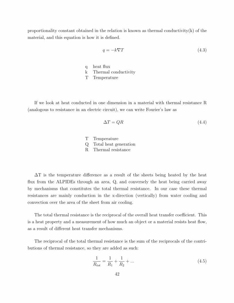
q heat fluxk Thermal conductivityT Temperature
If we look at heat conducted in one dimension in a material with thermal resistance R
(analogous to resistance in an electric circuit), we can write Fourier’s law as
∆T = QR (4.4)
T TemperatureQ Total heat generationR Thermal resistance
∆T is the temperature difference as a result of the sheets being heated by the heat
flux from the ALPIDEs through an area, Q, and conversely the heat being carried away
by mechanisms that constitutes the total thermal resistance. In our case these thermal
resistances are mainly conduction in the x-direction (vertically) from water cooling and
convection over the area of the sheet from air cooling.
The total thermal resistance is the reciprocal of the overall heat transfer coefficient. This
is a heat property and a measurement of how much an object or a material resists heat flow,
as a result of different heat transfer mechanisms.
The reciprocal of the total thermal resistance is the sum of the reciprocals of the contri-
butions of thermal resistance, so they are added as such:
1
Rtot
=1
R1
+1
R2
+ ... (4.5)
42

In our case this is thermal resistance from conduction and from convection:
Thermal resistance from conduction:
Rcond =12d
kAcond
(4.6)
12d Average distance to the heat source
k Thermal conductivityAcond Cross sectional area of conduction
Thermal resistance from convection:
Rconv =1
hAconv
(4.7)
h Convection coefficientAconv Area of convection
Here we will use two different convection coefficients for stationary air and for moderate
air flow from the air cooling system.
Thermal resistance from radiation is also a factor, but I will show why that can be
neglected in this case. Contributions from the additional material between the chips and the
carrier plate, like glue and flex cable material, is constant and can be added later [2].
43

4.1.3 Air convection coefficient
Figure 4.1: Illustrating free and forced air cooling convection in a double carbon trackinglayer
.
A tracking layer consists of two carbon sheets with ALPIDE chips, which means that each
carrier sheet has one side with ALPIDE chips facing the ALPIDEs on the other sheet. This
is shown in figure 4.1, where you can see the two sheets and the air gap in between them.
For the stationary air in the air gap inside the tracking layer we use a convection coefficient
of 8 Wm2K
. The other side of the carbon sheets, the outside of the layer, is hit by the forced
airflow coming from a slit below the tracking layers, as described and illustrated in the air
cooling design chapter. This convection from forced air is more complicated and we rely on
empirical formulas to get an estimated value.
We have used an approximation of forced air convection that is derived from a wind
44

tunnel experiment by Nusselt and Jurge [8].
h = 5.8 + 3.94v (4.8)
v Speed of air flow
The experiment looked at a 50cm× 50cm copper plate in a wind tunnel. This empirical
formula assumes homogeneous laminar flow and is valid for moderate air speeds. We want
to achieve a convection coefficient of 20 Wm2 K
for the air cooling, and this corresponds to an
air speed of 3.6 m/s, so that is the convection coefficient and/or air speed we have used in
the following calculations and simulations.
4.2 Other important formulas and equations
There are a few other theoretical concepts that should be mentioned which are closely con-
nected to the subjects of this thesis but will not be investigated as thoroughly as the thermal
properties.
4.2.1 Air volume flow and air speed
The convection from air cooling is dependent on air velocity, but to decide what kind of air
cooling system to buy or build, we need to know the required volumetric air flow. Fans move
a certain volume of air and the air speed is then dependent on the duct that it is connected
to, the cross sectional area that it flows through. In the tracking layer-end of our air cooling
system, the air exits through a slit or a nozzle, and this is where we need to control the
airspeed to get the desired cooling effect.
When trying to decide what would be required for a test setup and later, the prototype,
we want to find an air supply with the right volume flow. This will then be able to supply
us with the right air speed onto the carbon plates.
V = v × Aairflow × 3600s [m3
hour] (4.9)
45
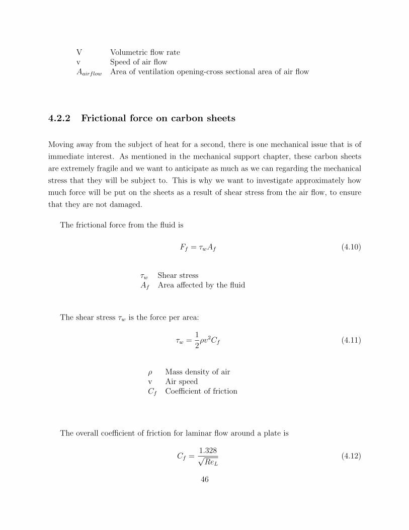
V Volumetric flow ratev Speed of air flowAairflow Area of ventilation opening-cross sectional area of air flow
4.2.2 Frictional force on carbon sheets
Moving away from the subject of heat for a second, there is one mechanical issue that is of
immediate interest. As mentioned in the mechanical support chapter, these carbon sheets
are extremely fragile and we want to anticipate as much as we can regarding the mechanical
stress that they will be subject to. This is why we want to investigate approximately how
much force will be put on the sheets as a result of shear stress from the air flow, to ensure
that they are not damaged.
The frictional force from the fluid is
Ff = τwAf (4.10)
τw Shear stressAf Area affected by the fluid
The shear stress τw is the force per area:
τw =1
2ρv2Cf (4.11)
ρ Mass density of airv Air speedCf Coefficient of friction
The overall coefficient of friction for laminar flow around a plate is
Cf =1.328√ReL
(4.12)
46

ReL is the global Reynolds number over the entire air path length along the plate:
ReL =vL
ν(4.13)
v Air speedL Air path lenghtν Kinematic viscosity of air
4.3 Calculations based on conduction and convection
4.3.1 Preliminary calculations of the effect of water cooling: gen-
eral heat equation
For the first calculation, one of our objectives was to look at the values of certain parameters
of the carbon sheets in order to decide what kind of material properties we would need
for our tracking layers, the effect of water cooling on this material and whether this water
cooling would be sufficient heat transfer. The thermal conductivity and the thickness of the
sheet are of particular interest, and are parameters that we have certain constraints on. The
reason for this is to make sure that the heat produced by the ALPIDEs do not result in a
temperature that would be problematic for the readout from the ALPIDEs themselves.
Here, I have made a simple model of temperature distribution throughout one carbon
sheet in one dimension. That is, how much the temperature changes in x-direction (verti-
cally) when a heat load is applied evenly over the whole volume of the sheet and the edges
are kept at a constant temperature. Of course this is our absolute worst case scenario where
all the chips are active and deliver their maximum power for long enough time that the
system reaches equilibrium. This is a highly unlikely case, but it is a good place to start
evaluating the thermal properties of our system.
These temperature difference calculations are derived from the heat conduction equation
(equation 4.2), as was explained in the previous section. This equation is modified and
simplified by the following boundary conditions.
47

• dTdt
= 0 - Steady state condition, no variation over time.
• k = constant - The material is homogenous and isentropic. The thermal conductivity
does not have any spatial dependency.
• ∂T∂y
= ∂T∂z
= 0 - One dimensional heat conduction. One of the unique properties of the
carbon fleece/paper sandwich.
This leaves us with the following equation, the Poisson equation in one dimension, which
is relatively easy to integrate:
∂2T
∂x2+qvk
= 0 (4.14)
qv Heat generated inside the volumek Thermal conductivity
Solving this for T (x) gives us
d2T
dx2= −qv
k= 0 (4.15)
dT
dx= −qv
k
wdx = −qv
kx+ C1 (4.16)
Evaluating this at the middle of the sheet x = 0, where T (x = 0) = Tmax due to the
symmetrical arrangement, shows that dTdx
= 0 −→ C1 = 0
T (x) =qvk
wxdx = −qv
k
x2
2+ C2 (4.17)
Then, to solve for C2 we evaluate T (x) at the water cooled edges at x = ±Lx
2with coolant
temperature T0. Lx is the height of the sheet.
T (x =Lx
2) = − qv
2k(Lx
2)2 + C2 = T0
−→ T (x) = − qv2kx2 +
qv2k
(Lx
2)2 + T0 (4.18)
48
The maximum temperature is at x = 0:
Tmax =qv2k
(Lx
2)2 + T0 (4.19)
This gives us the temperature difference between Tmax and T0:
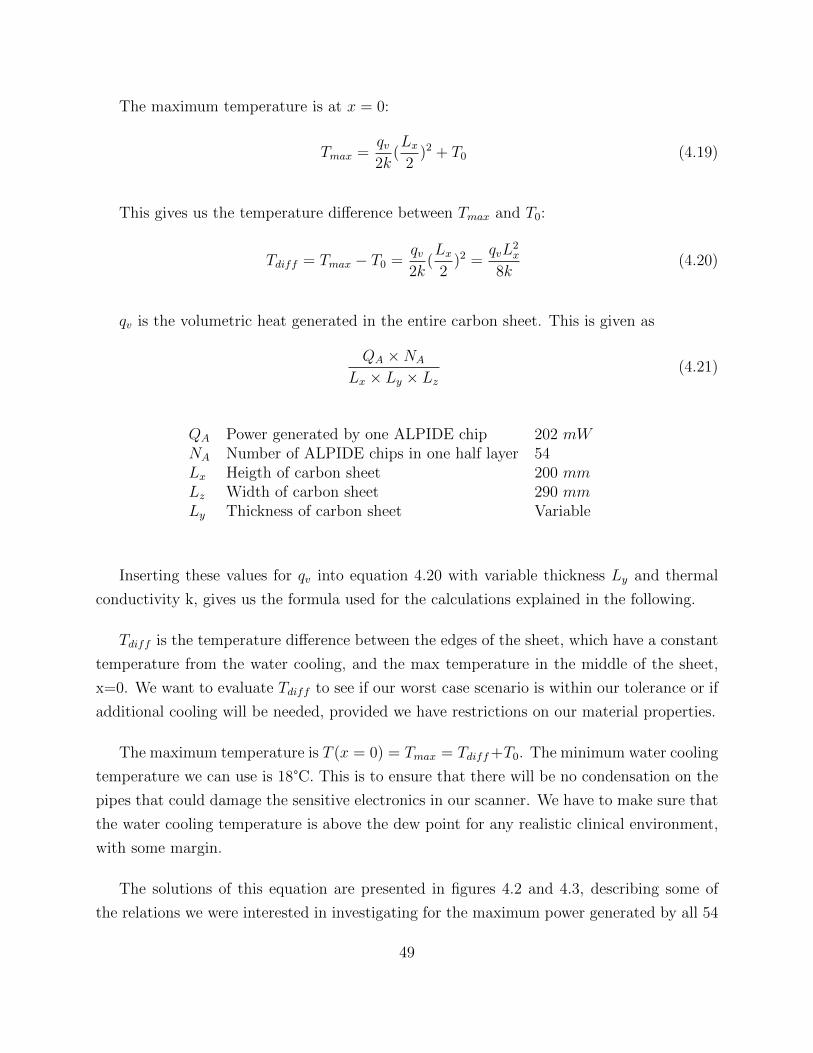
Tdiff = Tmax − T0 =qv2k
(Lx
2)2 =
qvL2x
8k(4.20)
qv is the volumetric heat generated in the entire carbon sheet. This is given as
QA ×NA
Lx × Ly × Lz
(4.21)
QA Power generated by one ALPIDE chip 202 mWNA Number of ALPIDE chips in one half layer 54Lx Heigth of carbon sheet 200 mmLz Width of carbon sheet 290 mmLy Thickness of carbon sheet Variable
Inserting these values for qv into equation 4.20 with variable thickness Ly and thermal
conductivity k, gives us the formula used for the calculations explained in the following.
Tdiff is the temperature difference between the edges of the sheet, which have a constant
temperature from the water cooling, and the max temperature in the middle of the sheet,
x=0. We want to evaluate Tdiff to see if our worst case scenario is within our tolerance or if
additional cooling will be needed, provided we have restrictions on our material properties.
The maximum temperature is T (x = 0) = Tmax = Tdiff +T0. The minimum water cooling
temperature we can use is 18°C. This is to ensure that there will be no condensation on the
pipes that could damage the sensitive electronics in our scanner. We have to make sure that
the water cooling temperature is above the dew point for any realistic clinical environment,
with some margin.
The solutions of this equation are presented in figures 4.2 and 4.3, describing some of
the relations we were interested in investigating for the maximum power generated by all 54
49

ALPIDEs. The first graph (figure 4.2) is the temperature difference as a function of thermal
conductivity for a few different values of sheet thickness. In the real prototype there are
constrictions on the thickness to keep in mind, to affect the particle beam energy as little
as possible in the tracking layers. The assumption is that the sheets will be approximately
0.2mm thick, but I have included a few values outside that just to see the relationship
between these parameters.
There is also a question of material availability when it comes to the larger values of k.
Carbon material with thermal conductivity of these larger values is quite hard to get for a
project of our scale, considering the budget and the small amount we would need. Therefore,
thermal conductivity of much more than 200 Wm K
is unlikely but again, larger values are
included for the sake of seeing this dependency. As is shown in this graph, the larger values
of k result in a smaller temperature difference, i.e. smaller maximum temperature as a
result of better heat conduction. The thickness of the sheet has a huge effect on temperature
difference for lower thermal conductivity values, in the range that are of interest to us.
50

Figure 4.2: The temperature difference, Tdiff in a carbon sheet of different thicknesses Ly,as a function of the thermal conductivity k
.
The second graph is describing the sheet thickness as a function of selected values of
temperature difference. This is plotted for different values of the thermal conductivity k.
We want to keep the ALPIDE chips from exceeding temperatures of 40°C. If we assume
the constant temperature as a result of the water cooling to be 18°C then this would mean
that Tdiff should not be more than 22°. This is not a hard cap on the function of the chips,
but the noise and threshold will increase with the temperature. Therefore we have this
tentative maximum temperature. Ideally we want to keep it much lower, as low as possible.
It is very clear from the figures that based on these calculations, all these constrictions and
considerations are hard to satisfy at the same time with only water cooling. If we were to
assume a thermal conductivity of 200 Wm K
and sheet thickness 0.2 mm, Tdiff is 23.5°.
51

Figure 4.3: Sheet thickness Ly as a function of the temperature difference, plotted for dif-ferent values of the thermal conductivity k
.
These calculations were made first for the aluminium layers in the calorimeter [11] and
then for the carbon tracking layers, before the air cooling was introduced. The results
presented in these graphs shows that some sort of additional cooling would be needed to
achieve the values of Tdiff that we need for the tracking layers to be working optimally.
With sufficient cooling effect from additional air cooling, the restrictions on carbon sheet
material are not a significant concern and this lets us stay within the range of acceptable
temperatures, even in the worst case scenario. This depends on what kind of results we see
from the air cooling effect.
We know the actual properties of the carbon fleece/paper sandwich that has been pro-
52
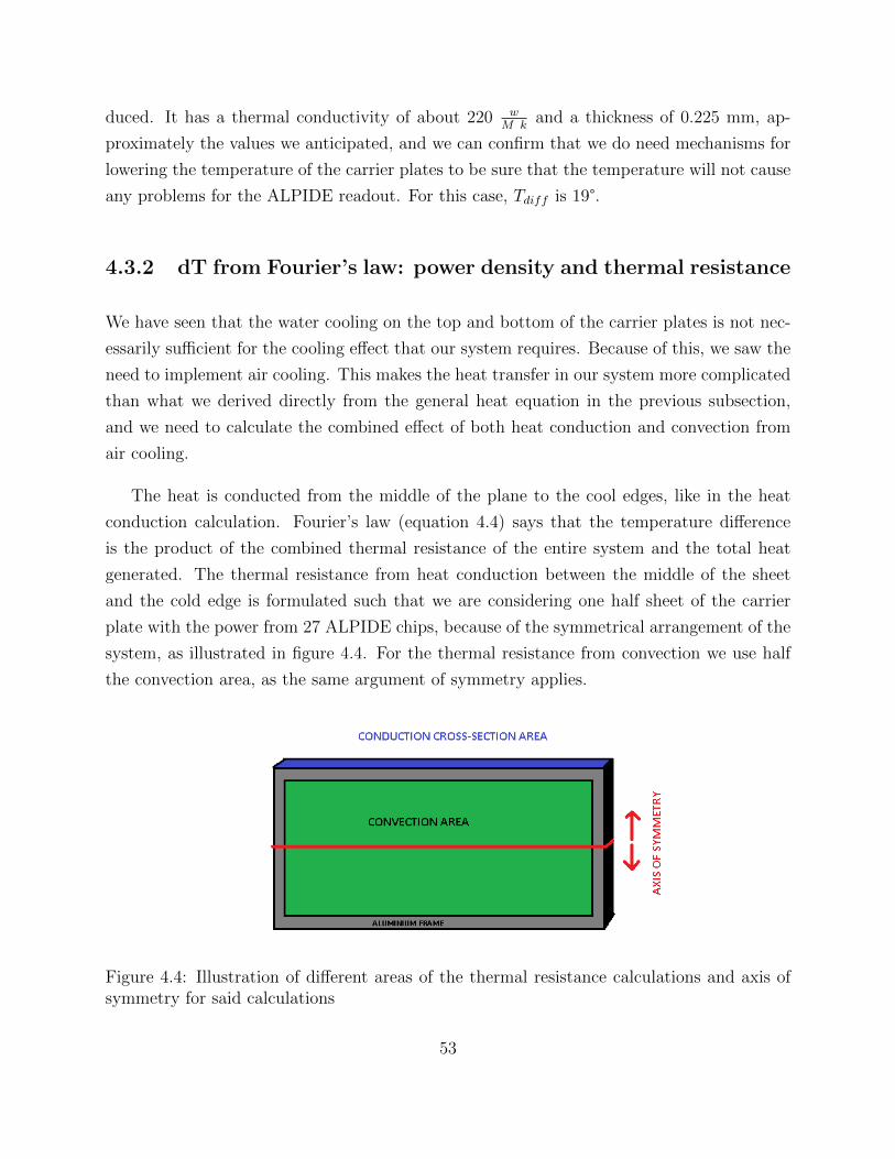
duced. It has a thermal conductivity of about 220 wM k
and a thickness of 0.225 mm, ap-
proximately the values we anticipated, and we can confirm that we do need mechanisms for
lowering the temperature of the carrier plates to be sure that the temperature will not cause
any problems for the ALPIDE readout. For this case, Tdiff is 19°.
4.3.2 dT from Fourier’s law: power density and thermal resistance
We have seen that the water cooling on the top and bottom of the carrier plates is not nec-
essarily sufficient for the cooling effect that our system requires. Because of this, we saw the
need to implement air cooling. This makes the heat transfer in our system more complicated
than what we derived directly from the general heat equation in the previous subsection,
and we need to calculate the combined effect of both heat conduction and convection from
air cooling.
The heat is conducted from the middle of the plane to the cool edges, like in the heat
conduction calculation. Fourier’s law (equation 4.4) says that the temperature difference
is the product of the combined thermal resistance of the entire system and the total heat
generated. The thermal resistance from heat conduction between the middle of the sheet
and the cold edge is formulated such that we are considering one half sheet of the carrier
plate with the power from 27 ALPIDE chips, because of the symmetrical arrangement of the
system, as illustrated in figure 4.4. For the thermal resistance from convection we use half
the convection area, as the same argument of symmetry applies.
Figure 4.4: Illustration of different areas of the thermal resistance calculations and axis ofsymmetry for said calculations
53

In this case, the temperature difference is between both water and air/room temperature,
T0, and the maximum temperature of the plate, Tmax. This is the temperature when we reach
the stable state with heating Q and cooling from as a result of total resistance Rtot. There is
no way for us to decouple the water and air temperatures, so this is one simplification of our
system which we will come back to. From Fourier’s law for heat conduction, we can express
the temperature difference as a function of the heat flux through the plane and the thermal
resistance of the plane. We will refer to this temperature difference as ∆T , to separate it
from the similar Tdiff from the previous calculation:
Tmax − T0 = ∆T = QRtot (4.22)
Q Total power generatedRtot Total thermal resistance
The total thermal resistance is given by the formula
1
Rtot
=1
Rcond
+1
Rconv1
+1
Rconv2
+1
Rrad
+1
Rconst
(4.23)
Rcond Thermal resistance from conductionRconv1 Thermal resistance from natural/free convectionRconv2 Thermal resistance from forced air convectionRrad Thermal resistance from radiationRconst Constant thermal resistance from glue, cable material etc.
The respective thermal resistances are calculated in the following. For conduction through
a cross-sectional area A, from equation 4.6, we insert these values:
12d 50mm
k 220 WmK
Acond 290× 0.225mm2
Like our previous calculation of the conductive plate with water cooling, the maximum
temperature will be in the middle of the sheet, at x = 0. The average distance from the
54

cold edge to the heat source is half the distance from the middle to the edge, from x = 0 to
x = Lx
2. This gives us
Rcond = 3.48K
W
Thermal resistance from free and forced convection is found by inserting the following
values into equation 4.7:
h1(free convection coefficient) 8 Wm2K
h2(forced convection coefficient) 20 Wm2K
Aconv 274× 85mm2
The area cooled by convection is 274mm x 170mm. This is because the spacers that
constitute the frame for the tracking layers and the support for the water cooling pipes
envelops a few centimeters of the carrier plates, as shown in figure 4.4. We use half of this
area as our convection area in this calculation.
Rconv1 = 5.37K
W
Rconv2 = 2.15K
W
Thermal resistance from radiation, derived from Stefan-Boltzmann’s law:
1
ε · σ · Arad(T 2alpide + T 2
0 )(Talp + T0)(4.24)
ε Emissivity(we assume black body radiation) 1σ Stefan Boltzmann’s constant 5.67× 10⁻⁸ W
m2·K4
Arad Radiative surface, surface of ALPIDE chips 450 mm2 × 27Talpide Temperature of ALPIDEs(using 40°C for worst case scenario) 313 KT0 Room temperature 293 K
Rrad = 13.03K
W
55

Thermal resistance from constant factors, Rconst, is not included at this time. This results
in a constant temperature difference which can be added at a later time when this has been
investigated further.
Table 4.1: Results from thermal resistance calculations. Contribution from eachcooling effect, their reciprocals and the running total resistance.
R 1R
Rtot
Conduction 3.48 0.29 3.48Free convection 5.37 0.19 2.11Forced convection 2.15 0.47 1.07Radiation 13.03 0.08 0.98
In table 4.1 we have calculated all the individual thermal resistances and their reciprocals,
which are added to find the total thermal resistance (equation 4.23). The third column is the
running total thermal resistance from top to bottom. As we can see from this, the thermal
resistance from radiation contributes very little to reducing the total thermal resistance and
can be neglected in our case.
Now that we have the total thermal resistance, we can put it back into the formula based
on Fourier’s law. The power consumption of each ALPIDE chip is estimated to be 202 mW
for the most common operating conditions of a pCT scan [12]. For our half sheet with 27
chips, this makes for a total power of 5.45 W.
The calculated temperature differences for different scenarios of cooling mechanisms are
written in table 4.2 below
Table 4.2: Results for ∆T
Cooling mechanism ∆TConduction 19Conduction with free convection 11.52Conduction with free and forced convection 5.81
The temperature difference with only conduction from the edges cooled by water, is
the same as the previous calculation we did. If we add the free convection, this should
be a slightly more realistic model of the scenario without air cooling. ∆T with all three
56
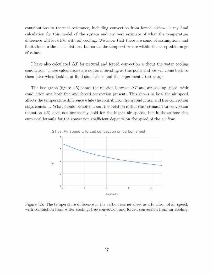
contributions to thermal resistance, including convection from forced airflow, is my final
calculation for this model of the system and my best estimate of what the temperature
difference will look like with air cooling. We know that there are some of assumptions and
limitations to these calculations, but so far the temperature are within the acceptable range
of values.
I have also calculated ∆T for natural and forced convection without the water cooling
conduction. These calculations are not as interesting at this point and we will come back to
them later when looking at fluid simulations and the experimental test setup.
The last graph (figure 4.5) shows the relation between ∆T and air cooling speed, with
conduction and both free and forced convection present. This shows us how the air speed
affects the temperature difference while the contribution from conduction and free convection
stays constant. What should be noted about this relation is that this estimated air convection
(equation 4.8) does not necessarily hold for the higher air speeds, but it shows how this
empirical formula for the convection coefficient depends on the speed of the air flow.
Figure 4.5: The temperature difference in the carbon carrier sheet as a function of air speed,with conduction from water cooling, free convection and forced convection from air cooling
.
57
4.4 Other important calculations
4.4.1 Air volume flow
The volume flow of the cooling system is a simple, but important calculation. The air coming
out of the slits in our cooling system is 28 m3
hour, if we want an air speed of 3.6m
sonto the
tracking layers. Because of this, we should have an air supply that can give at least 60 m3
hour,
taking into consideration the uncertainties we have in our current model of the air cooling
system. There is pressure drop and friction in the vents, turbulence and a lot more on the
subject of fluid dynamics which is outside the scope of this thesis.
4.4.2 Frictional force
In the previous section, we presented the frictional force from laminar air flow on a plate
in equation 4.10. Inserting the convection area and the following constants to calculate the
shear stress (equations 4.11, 4.12 and 4.13):
Area affected by fluid 274× 170 mm2
Air density 1.225 kgm3
Air speeed 3.6 ms
Length of air path 170 mm
Kinematic viscosity of air 15.06× 10⁻⁶ m2
s
This gives us the frictional force on the carbon sheet:
Ff = 0.00244 N
4.4.3 Fan noise and vibration
This is not a direct calculation, but we have investigated what kind of fans are available for
our intended use. Assuming that there is some uncertainty in the volumetric flow calculation,
we need a fan that delivers double the volume flow that we have calculated to achieve the
58

required air speed. This means we want at least 0.93 m3
min. The fans that are the closest to
these specifications have a max volume flow of 1 m3
minat 4000 rpm. The noise from these is
supposed to be 40.6 dB, and the fan speed indicates that the frequency of this noise is 66.7
Hz.
This is a representative example but it is too early to tell which kind of ventilation or fan
will be used as air supply for the pCT. This thesis focuses primarily on the thermal aspects
of the cooling system, and therefore will conclude any further on this subject.
4.5 Simulations
Another method we use to model the thermal properties of the tracking system is simulations.
The student version of a sophisticated simulation/CAD software called ANSYS was the
best option available for this. The results from these simulations gives us another set of
temperature calculations for comparison and provides us with better visualizations of our
model and its temperature distribution. ANSYS has a modular interface, in which you work
from a virtual Workbench environment which implements and combines different software
for data input, simulation, CAD drawing and more. We will only be looking at the specific
functions of the software used for the simulations in question, but the interface with its
variety of components is demonstrated in figure 4.6 below.
59

Figure 4.6: An example of how the Workbench interface looks in ANSYS student version.
We look at results from two different simulation modules in ANSYS. In both cases, the
models for the simulations have been made in a CAD software called DesignModeler. The
first one is a steady-state thermal simulation that takes in boundary conditions and thermal
properties to solve for e.g. temperature or heat flux over the area of the plate. For the
second type of simulation, we use Fluent, a fluid simulation that physically models the flow
of air and how it affects the model. In this case, the speed of the air flow itself is entered as
input instead of a thermal property like convection. In each case we will look at comparisons
between the simulation results and calculations from the previous section. These methods
will be compared to experimental measurements in chapter 5.
60

4.5.1 Simulation models
There are three different models that we want to simulate:
• The carbon tracking layer model is an aluminium sheet of 290mm×200mm×0.225mm
with a thermal conductivity of 220 Wm K
.
• Aluminium (Al1050) model for cooling tests, made in Utrecht with dimensions
290mm × 200 × 0.2mm. Al 1050 has thermal properties that are quite similar to
our carbon material.
• The third model is a smaller aluminium plate that was built in the lab in Bergen to
test the effect of air cooling on a heated aluminium plate. This is a smaller, simpler
setup consisting of a plate with heating tape on the backside, air flowing onto the front
of the plate and no water cooling. With this model, we can compare simulation results
to real-life measurements, to get a sense of how realistic these simulations are. This
experimental setup will be described more in-depth in chapter 5.
4.5.2 Steady state thermal simulations
For both the carbon layer and the aluminium cooling test layer I have used a thermal
conductivity of 220 Wm K
, a total heat load of 10.9 W, which corresponds to 54 chips that
produce 202 mW each. In figure 4.7 below, you can see the setup for the simulation case
that is closest to the calculations. Here, the heat load is distributed over the whole surface
and the water cooling and air has the same temperature, T0. In this case T0 is 25 °C but the
actual value of T0 does not affect the calculation of the temperature difference.
61

Figure 4.7: An example of how the setup for the first set of steady-state simulations look.
Figure 4.8: Steady-state simulation of temperature of the carbon carrier plate with watercooling and heat load distributed over the whole plate
62

The simulations for this heat distribution is run first with conduction from water cooling
only, then with free convection and at last, forced convection from air flow corresponding to
a convection coefficient of 20 Wm2 K
. We can look at the temperature distribution but even
more importantly, the total temperature difference. An example of what the simulation
results looks like is displayed in figure 4.8.
These simulations shows a temperature difference of 19, 11.28 and 5.48 degrees for the
different thermal resistances. This is very close to the calculated values, which are shown in
table 4.3. This means that the results of the calculations are comparable to the simulations
results. When we narrow in towards a more realistic model of the carrier plate, we will see
how our assumptions in the more idealized calculations differ from the real system.
Table 4.3: Comparison of calculated values to simulation results
Calculated ∆T Simulated ∆TWater cooling only 19 19Water cooling and free convection 11.52 11.28Water cooling, free convection and air cooling 5.81 5.48
The same type of simulation is run for the heat generated inside areas resembling the
9-chip ALPIDE strings. Both of these have been run with the same temperature for water
and air cooling, like the calculations, and 18°C water temperature and 20°C air/ambient
temperature. This has all been repeated for the Utrecht cooling test model as well which
will give us some information about the plate thickness dependency and can be compared
when tests are run on this setup.
The results from these simulations compared to their corresponding calculations, using
Fourier’s law (equation 4.22) calculating the temperature difference ∆T in the previous
section, are shown in the graphs below in figures 4.9 and 4.10.
63

(a) Same temperature for water and air
(b) Minimum water temperature we can use
Figure 4.9: Comparison of the calculated values to the simulations using the carbon trackingmodel for the pCT
64
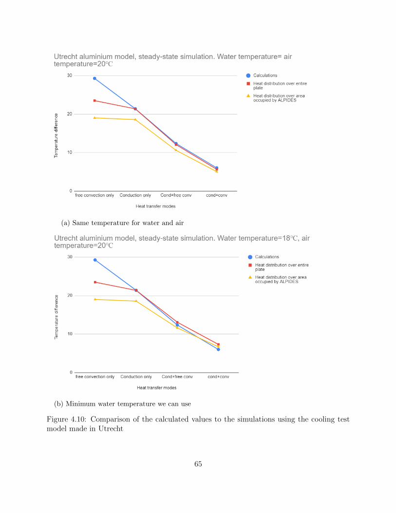
(a) Same temperature for water and air
(b) Minimum water temperature we can use
Figure 4.10: Comparison of the calculated values to the simulations using the cooling testmodel made in Utrecht
65
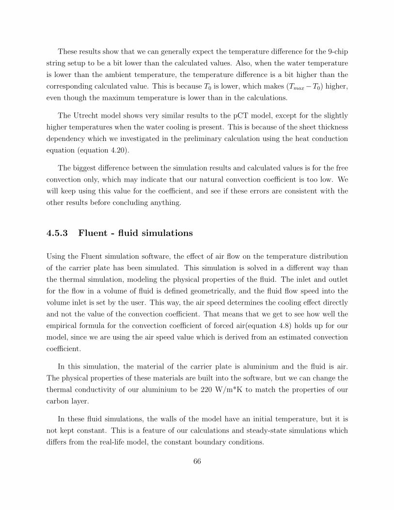
These results show that we can generally expect the temperature difference for the 9-chip
string setup to be a bit lower than the calculated values. Also, when the water temperature
is lower than the ambient temperature, the temperature difference is a bit higher than the
corresponding calculated value. This is because T0 is lower, which makes (Tmax−T0) higher,
even though the maximum temperature is lower than in the calculations.
The Utrecht model shows very similar results to the pCT model, except for the slightly
higher temperatures when the water cooling is present. This is because of the sheet thickness
dependency which we investigated in the preliminary calculation using the heat conduction
equation (equation 4.20).
The biggest difference between the simulation results and calculated values is for the free
convection only, which may indicate that our natural convection coefficient is too low. We
will keep using this value for the coefficient, and see if these errors are consistent with the
other results before concluding anything.
4.5.3 Fluent - fluid simulations
Using the Fluent simulation software, the effect of air flow on the temperature distribution
of the carrier plate has been simulated. This simulation is solved in a different way than
the thermal simulation, modeling the physical properties of the fluid. The inlet and outlet
for the flow in a volume of fluid is defined geometrically, and the fluid flow speed into the
volume inlet is set by the user. This way, the air speed determines the cooling effect directly
and not the value of the convection coefficient. That means that we get to see how well the
empirical formula for the convection coefficient of forced air(equation 4.8) holds up for our
model, since we are using the air speed value which is derived from an estimated convection
coefficient.
In this simulation, the material of the carrier plate is aluminium and the fluid is air.
The physical properties of these materials are built into the software, but we can change the
thermal conductivity of our aluminium to be 220 W/m*K to match the properties of our
carbon layer.
In these fluid simulations, the walls of the model have an initial temperature, but it is
not kept constant. This is a feature of our calculations and steady-state simulations which
differs from the real-life model, the constant boundary conditions.
66
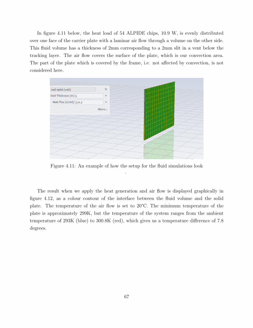
In figure 4.11 below, the heat load of 54 ALPIDE chips, 10.9 W, is evenly distributed
over one face of the carrier plate with a laminar air flow through a volume on the other side.
This fluid volume has a thickness of 2mm corresponding to a 2mm slit in a vent below the
tracking layer. The air flow covers the surface of the plate, which is our convection area.
The part of the plate which is covered by the frame, i.e. not affected by convection, is not
considered here.
Figure 4.11: An example of how the setup for the fluid simulations look.
The result when we apply the heat generation and air flow is displayed graphically in
figure 4.12, as a colour contour of the interface between the fluid volume and the solid
plate. The temperature of the air flow is set to 20°C. The minimum temperature of the
plate is approximately 299K, but the temperature of the system ranges from the ambient
temperature of 293K (blue) to 300.8K (red), which gives us a temperature difference of 7.8
degrees.
67
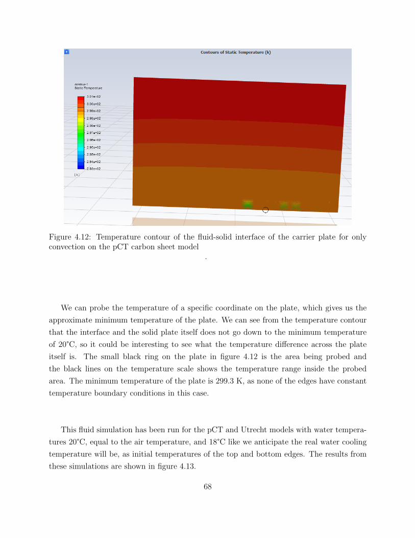
Figure 4.12: Temperature contour of the fluid-solid interface of the carrier plate for onlyconvection on the pCT carbon sheet model
.
We can probe the temperature of a specific coordinate on the plate, which gives us the
approximate minimum temperature of the plate. We can see from the temperature contour
that the interface and the solid plate itself does not go down to the minimum temperature
of 20°C, so it could be interesting to see what the temperature difference across the plate
itself is. The small black ring on the plate in figure 4.12 is the area being probed and
the black lines on the temperature scale shows the temperature range inside the probed
area. The minimum temperature of the plate is 299.3 K, as none of the edges have constant
temperature boundary conditions in this case.
This fluid simulation has been run for the pCT and Utrecht models with water tempera-
tures 20°C, equal to the air temperature, and 18°C like we anticipate the real water cooling
temperature will be, as initial temperatures of the top and bottom edges. The results from
these simulations are shown in figure 4.13.
68
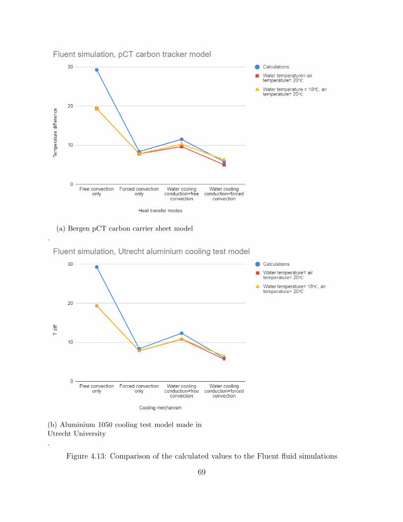
(a) Bergen pCT carbon carrier sheet model
.
(b) Aluminium 1050 cooling test model made inUtrecht University
.
Figure 4.13: Comparison of the calculated values to the Fluent fluid simulations
69
4.5.4 Comparing calculations to results from simulations
Now we have seen the results from the calculations and simulations for the pCT carbon
tracking layers and the Utrecht aluminium tracking layer test model. There are many un-
certainties to consider as a result of the limitations of the calculations and the simulation
software.
We know that these results are different from what we can expect to see when this
complex system of mechanical and thermally coupled parts is tested in reality. We will look
into the general results from the calculations and simulations and sum up the most important
uncertainties from this modeling. There are also some things that should be mentioned for
the continued investigation into the modeling of the tracking layers beyond the scope of this
thesis.
From the results of this chapter, we can conclude:
• The key numbers from the calculations seem to agree with the simulation results. The
calculations are not very far away from the much more sophisticated calculations made
by the simulation software.
• The biggest difference is the calculations vs simulations of the case with only free
convection. This is not a vital result for us in and of itself but it indicates that our
calculation of the value we use for natural convection coefficient might be wrong in
this case.
• Generally, the temperature differences and maximum temperatures are lower in the
simulation results than the calculations.
With all this said, some big uncertainties still prevail. The simulations and calculations
are both very idealized scenarios so naturally there are some things that are not considered
here at all.
• The convection coefficient calculation assumes laminar air flow, the same goes for the
fluid simulation in Fluent. This makes sense, seeing that the fluid simulation results
match our calculated values. In the real life case, on the other hand, we have reason
to believe that the flow will be turbulent to some degree. There is no way of knowing
how these results will look before assembling the test setup, as turbulence makes the
modeling of fluid dynamics more complicated.
70
• There is thermal resistance that I have summed up in the calculation as a constant
thermal resistance due to mechanical coupling between the cooling water, pipes, solder,
cooling block and onto the carrier plate. Also there is a difference in the convection
capabilities of laminar and turbulent water flow. This is not a significant problem with
the calculations, as it contributes a constant temperature difference that can be added
later on [2].
• When modeling the cooling systems, both air and water supply with tubes, soldering
and cooling blocks, there are several unknown factors like pressure drop due to friction
and turbulence. These things can be modeled, but it is outside the main subjects of
this thesis and have thus only been mentioned in passing. These things are important
when it comes to anticipating how much the experimental measurements will differ
from our results.
4.6 Summary and conclusions
The results from the calculations and simulations can be summed up as follows:
• The calculation derived from the general heat equation indicated that water cooling
was not sufficient for optimal operation and readout of the ALPIDEs.
• The calculation based on Fourier’s law (equation 4.22) which factored in other sources
of thermal resistance, most importantly air cooling, showed that with a convection
coefficient of 20 Wm2 K
the temperature difference would be kept low enough even for the
maximum heat generation possible.
• The steady-state simulations confirmed that our calculated values were representative
for the system that we wanted to model.
• The fluid simulations showed that our modeling of the air convection and cooling was
a good approximation.
4.6.1 Comparing simulations to experimental results
Moving forward, we would like to compare these models to experimental measurements. In
the next chapter we look at an experimental setup and temperature measurements from
71

this experiment. The setup has its own inherent flaws and this will be discussed in light
of corresponding calculations and simulations, how these things relate and deviate from
each other. The discussions in this section will then be brought back up in light of these
comparisons going into the last chapter.
72

Chapter 5
Experimental results
For the final part of this thesis, we have an experimental setup for temperature measurements
that may give us some insight into how the simulations hold up compared to the reality of
the cooling of the pCT. Ideally we would like to measure the real carbon tracker layer, or
the aluminium tracker layer made in Utrecht for this exact purpose. Unfortunately, due to
travel bans and lockdowns during the Covid-19 pandemic, everything has taken more time
than expected and the Utrecht model has not yet come to Bergen for testing.
We made a small scale test setup for air cooling only to have some measurements to
compare to the calculations and simulations. This means that we have to compare this to
another set of calculations and simulations, for the small-scale air cooling test model. We
will look back on the issues we presented with the simulations and calculations from the
previous chapter in light of this comparison.
5.1 Experimental setup
Equipment:
• Two plates of Aluminium 6062, dimensions 121mm × 52mm × 0.5mm, thermal con-
ductivity 170 Wm K
.
73

• One heating tape, 100mm× 25mm, max power 4W at 12V according to factory refer-
ence.
• One fan, mounted on a metal stand.
• Cardboard and tape for a makeshift “vent” with a slit for air flow.
The setup and assembly is quite simple. The heating tape is glued onto one of the
aluminium plates, as you can see in figure 5.1a. With four small plastic screws, one in each
corner, this is attached to the second aluminium plate. This makes an air gap of about 1.5
cm on the side that has the heating tape to make it stand up, because we want to blow air
from below, parallel to the heated plate.
The fan is sitting in the bottom of a cardboard vent/funnel, as seen in figure 5.1b. This
way it is blowing air upwards towards the slit. The airflow at different positions above the
fan is very uneven, so the funnel was an attempt to even that out a bit. We will get back to
how successful that proved to be. The fan has a max voltage of 12 V. Later we will look at
how this translates to different air speeds in the different positions across the outlet.
(a) Aluminium plate with heating tape
.
(b) Fan sits at the bottom of the cardboard vent
.
Figure 5.1
At the top of the cardboard funnel there is a slit, approximately 120mm long, which
can be seen in figure 5.2a. The width of the slit is corrected with black tape, so that it is
74
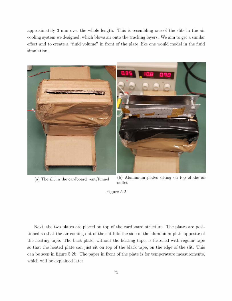
approximately 3 mm over the whole length. This is resembling one of the slits in the air
cooling system we designed, which blows air onto the tracking layers. We aim to get a similar
effect and to create a “fluid volume” in front of the plate, like one would model in the fluid
simulation.
(a) The slit in the cardboard vent/funnel (b) Aluminium plates sitting on top of the airoutlet
Figure 5.2
Next, the two plates are placed on top of the cardboard structure. The plates are posi-
tioned so that the air coming out of the slit hits the side of the aluminium plate opposite of
the heating tape. The back plate, without the heating tape, is fastened with regular tape
so that the heated plate can just sit on top of the black tape, on the edge of the slit. This
can be seen in figure 5.2b. The paper in front of the plate is for temperature measurements,
which will be explained later.
75

5.2 Measurements
To measure the airspeed, I have used a testo Smart Probe anemometer. An anemometer is a
device used to measure air velocity. This particular probe is a hot wire anemometer with an
adjustable shaft with a hole perpendicular to the shaft, that has a conducting wire inside it.
The wire is heated by electrical current and when the hot wire is placed in the air stream,
the heat is transferred from the wire to the fluid. The resulting resistance of the wire is used
to measure the flow rate of the fluid.
The anemometer is mounted on a stand, measuring the airflow at 12 different positions
along the slit with 1 cm intervals, 1.5 cm above the outlet, as can be seen in figure 5.3.
Figure 5.3: Air speed measurements above the outlet.
The result from these measurements can be seen in fig 5.4. The temperature is measured
for fan voltages ranging from 6V, as low as possible, in 2V intervals up to 12 which is the
max voltage of the fan. As is apparent from this graph, there is a big variation of air speeds
across the slit so I will use the average speed for each voltage when trying to model this for
76

the calculations and simulations. The issues and challenges with this will be discussed when
we evaluate the results.
This variation is due to air speed variation at different positions above the fan and the
vent/funnel did not even out the airflow as much as I had hoped. Also, the airflow is
turbulent and even if we put some material inside the funnel to diffuse and even out these
variations, the resulting cooling effect would be approximately the same.
Figure 5.4: Measured air speed along the slit (z-direction), 1.5 cm above the outlet. Measurefor four different voltages on the fan
.
5.2.1 Temperature measurements
The FLUKE 80T-IR infrared (IR) temperature probe connected to a multimeter has been
used to measure the temperature of the plate. This probe is pointed by hand at an object
and reads out the black-body radiation emitted by the object as a temperature in degrees
Celsius, when we apply a voltage from the multimeter. This can be seen in figure 5.5a. One
77

issue with the IR probe is when pointing it at a highly reflective surface like an aluminium
plate it does not register any emitted infrared radiation, so one would have to put some
non-reflective material in front to solve this issue. I have used white paper in front which is
fastened with kapton, heat resistant tape, to minimize the effect this has on the heat transfer
effect.
(a) Temperature measurement with IR probe
(b) Test setup aluminium plate with paper infront and position markers
Figure 5.5
The temperature was measure at five different locations on the plate, to see if there was
any significant spatial variation in the temperature. The z-coordinates (horizontally) that
are marked are at 2, 4 and 6 cm and at the 6 cm mark, the x-coordinates (vertically) are
1.5, 2.5 and 3.5 cm. You can see the approximate dimensions of the plate and the marked
positions on the assembled test setup in figure 5.5b.
Each position has been measured five times for each setting, to cancel out some measure-
ment uncertainty. The process has been as follows:
78

• Turn on the heating tape with voltage 4, 8 or 11.8 volts.
• Turn on the fan on the lowest setting, 6 volts. Wait until the temperature stabilizes.
• Measure five times for each position.
• Repeat for the remaining fan settings.
There are several sources of uncertainty in this experiment. We will have a brief look at
what they are before we start discussing the results from the measurements.
5.2.2 Sources of uncertainty
There are some factors of uncertainty in comparing the experiment to a theoretical model
or simulation:
• The airspeed is very uneven and the airflow is far from laminar.
• The IR-probe is hand held and therefore subject to human error.
• There are a lot of unknown thermal resistances which are hard to model. The way the
heating tape is glued onto the aluminium plate, the contact between the plate and the
material it is standing on, the paper in front of the plate for measurement are at least
some of them.
5.3 Results
The results from the measurements are gathered in a table, like in figure 5.6. Here, T0 (T0)
is the ambient temperature and the initial temperature of the plate and T max (Tmax) is the
stable temperature in the middle of the plate, with the heat load generated by the heating
tape at the given voltage. The temperatures are measured five times for each coordinate on
the plate.
79
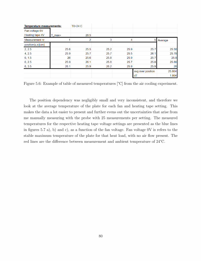
Figure 5.6: Example of table of measured temperatures [°C] from the air cooling experiment.
The position dependency was negligibly small and very inconsistent, and therefore we
look at the average temperature of the plate for each fan and heating tape setting. This
makes the data a lot easier to present and further evens out the uncertainties that arise from
me manually measuring with the probe with 25 measurements per setting. The measured
temperatures for the respective heating tape voltage settings are presented as the blue lines
in figures 5.7 a), b) and c), as a function of the fan voltage. Fan voltage 0V is refers to the
stable maximum temperature of the plate for that heat load, with no air flow present. The
red lines are the difference between measurement and ambient temperature of 24°C.
80
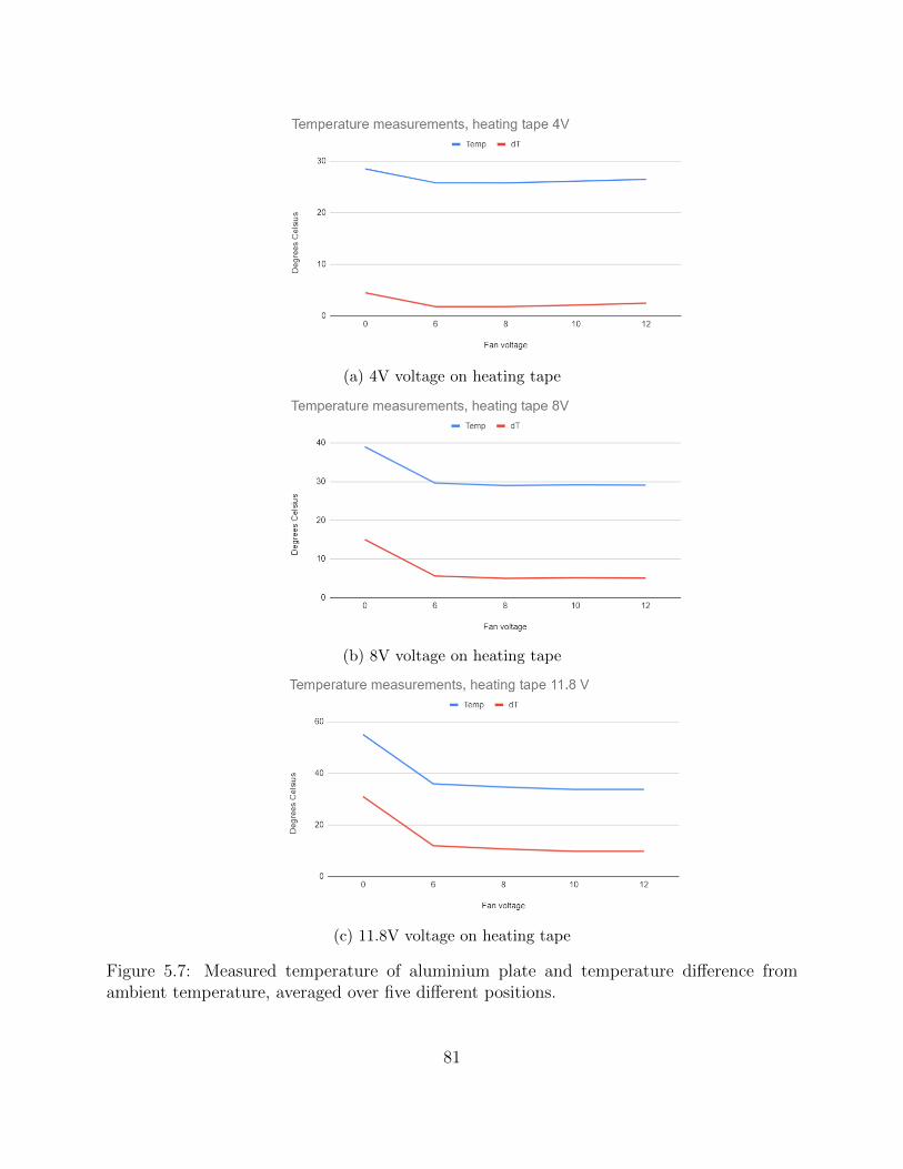
(a) 4V voltage on heating tape
(b) 8V voltage on heating tape
(c) 11.8V voltage on heating tape
Figure 5.7: Measured temperature of aluminium plate and temperature difference fromambient temperature, averaged over five different positions.
81

5.3.1 Observation from measurements
The cooling effect of an air stream onto the aluminium plate is significant, as seen in the
temperature difference from 0V to 6V on the fan. The effect of further increasing the voltage
on the fan, and in turn the air speed, is not as big as we would expect from the measurements
of the air speeds and the convection coefficient we calculate from that. This effect is also a
bit inconsistent, for the 4V heating tape setting, the temperature increases a bit when we
increase the air speed, opposite of what we would expect. This is due to the relatively small
differences in temperature and uncertainties in measurement.
5.3.2 Expectations from future measurements
When the tracking layer replica model from Utrecht is assembled, we can expect to see a
bit more consistent results and get measurements that fit our calculations and simulations
better. The layers will be mounted properly with the spacers and water cooling, suspended
on rods and not touching anything else that might affect the thermal resistance. Also, the
heat conduction from water cooling should be easier to predict than convection because the
behaviour of the fluid is harder to predict than the plate material. The proper test setup
will have an air cooling system similar to the one we designed for the pCT. This will make
the air flow more controlled, less turbulent and closer to the simulated model.
5.4 Comparing measurements to calculations and sim-
ulations
For comparison, all the calculations and simulations that I did in the previous chapter
has been modified for my experimental model. These results are presented as graphs and
compared to the corresponding results from my measurements.These will be presented in
the same order as before, first the calculations, then the steady state simulation and lastly
the fluid simulation.
82

5.4.1 Calculations with Fourier’s law
The first calculation is Fourier’s law (equation 4.22) with resistance from free and forced
convection, without any conduction or radiation. This is shown in figure 5.8. A voltage of
12V on the heating tape gives its maximum of 4W power according to the data sheet from
the manufacturer. When applying 11.8V on the heating tape, it is drawing 0.35A of current.
This means that the actual power drawn by the heating tape for this setting is 4.13W. With
8V voltage it is drawing 1.92 W and for the 4V setting, 0.48W.
There is no constant temperature as boundary conditions, only convection. For fan
voltage setting 0V I have used free convection on both sides of the plate, while for the other
fan settings there is one side with free convection and one side with coefficient calculated
from forced convection previously, in chapter 4 with equation 4.8.
The heating tape measures 100mm × 25mm which is approximately the area of 5.5
ALPIDE chips. Drawing a maximum of 202mW each, this means that the corresponding
area of ALPIDEs would draw 1.11W. This is somewhere between the 4V and 8V setting on
the heating tape we have used.
We see immediately that the temperatures are higher than the measured values, with the
temperature difference for the highest power setting being 43.8 degrees. This would mean
that the temperature of the plate is 67.8 degrees. This was expected, as there are several
sources of thermal resistance that we did not consider in this case.
83
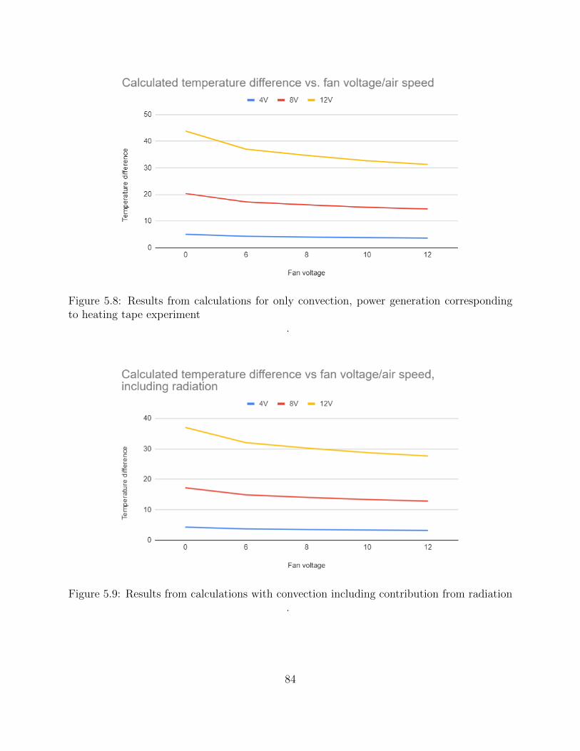
Figure 5.8: Results from calculations for only convection, power generation correspondingto heating tape experiment
.
Figure 5.9: Results from calculations with convection including contribution from radiation.
84
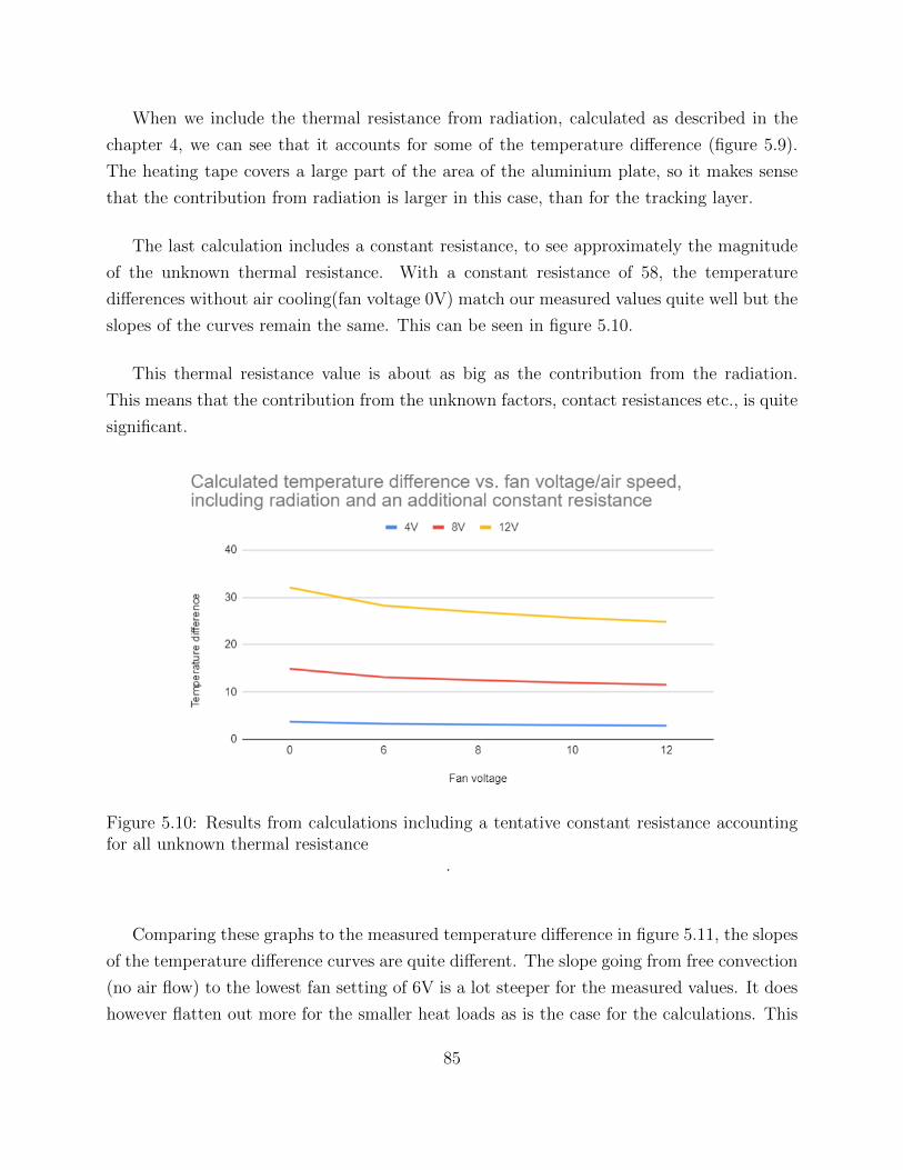
When we include the thermal resistance from radiation, calculated as described in the
chapter 4, we can see that it accounts for some of the temperature difference (figure 5.9).
The heating tape covers a large part of the area of the aluminium plate, so it makes sense
that the contribution from radiation is larger in this case, than for the tracking layer.
The last calculation includes a constant resistance, to see approximately the magnitude
of the unknown thermal resistance. With a constant resistance of 58, the temperature
differences without air cooling(fan voltage 0V) match our measured values quite well but the
slopes of the curves remain the same. This can be seen in figure 5.10.
This thermal resistance value is about as big as the contribution from the radiation.
This means that the contribution from the unknown factors, contact resistances etc., is quite
significant.
Figure 5.10: Results from calculations including a tentative constant resistance accountingfor all unknown thermal resistance
.
Comparing these graphs to the measured temperature difference in figure 5.11, the slopes
of the temperature difference curves are quite different. The slope going from free convection
(no air flow) to the lowest fan setting of 6V is a lot steeper for the measured values. It does
however flatten out more for the smaller heat loads as is the case for the calculations. This
85
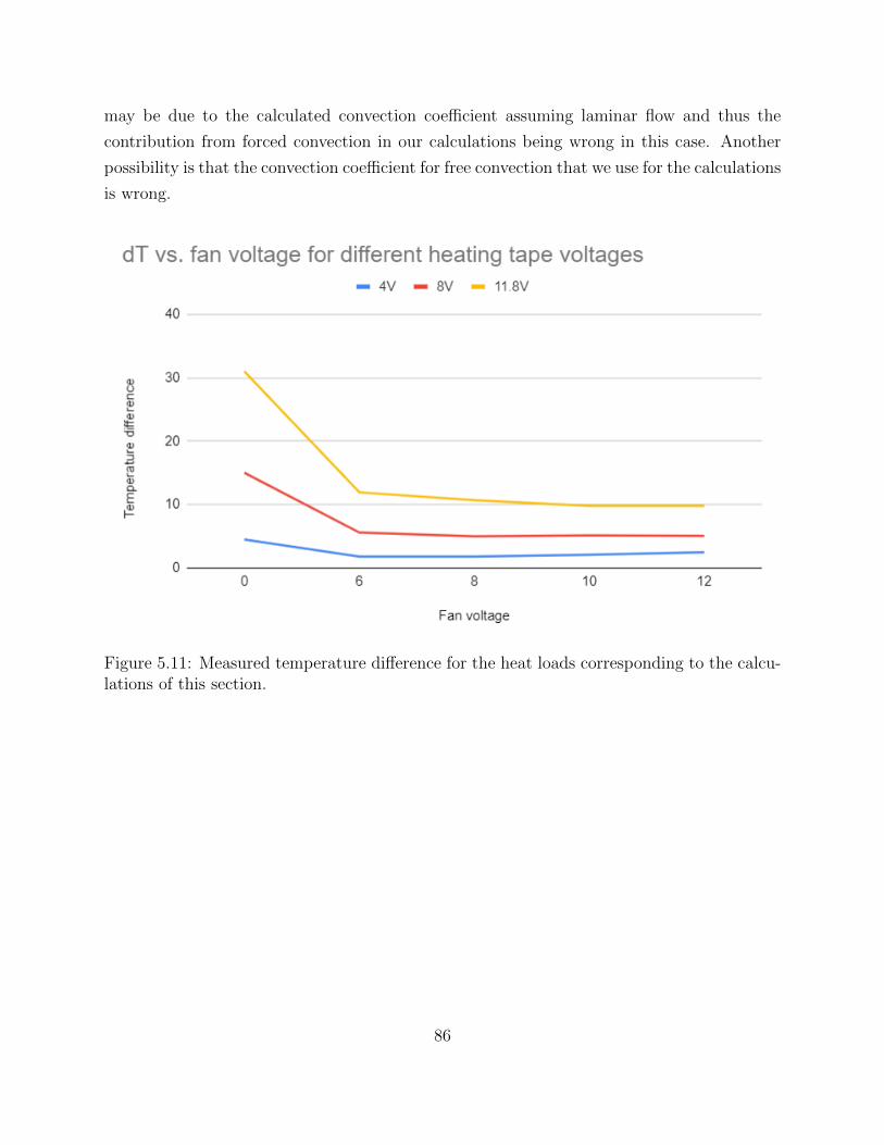
may be due to the calculated convection coefficient assuming laminar flow and thus the
contribution from forced convection in our calculations being wrong in this case. Another
possibility is that the convection coefficient for free convection that we use for the calculations
is wrong.
Figure 5.11: Measured temperature difference for the heat loads corresponding to the calcu-lations of this section.
86

5.4.2 Simulations
For further comparison, we have simulated this experimental setup in ANSYS. The first
simulation is a steady-state thermal simulation with the heat load distributed over an area
corresponding to the area of the heating tape. We have applied free convection to both sides
and then changed the convection coefficient on one side to match the forced convection from
our different fan voltage settings, same as for the calculations. The solution to one of the
simulations is shown in figure 5.12.
Figure 5.12: Example of steady state simulation solution, for 4.13W heat load and convectioncoefficient h=17.6
.
Here we have also used the forced convection coefficient that is calculated from the
measured airspeed. The temperatures in this case are also higher than our measured results
and looks very similar to our calculation without radiation and additional resistance (figure
5.8). The results from the steady state simulations for the different heat loads are shown in
the graph in figure 5.13.
87
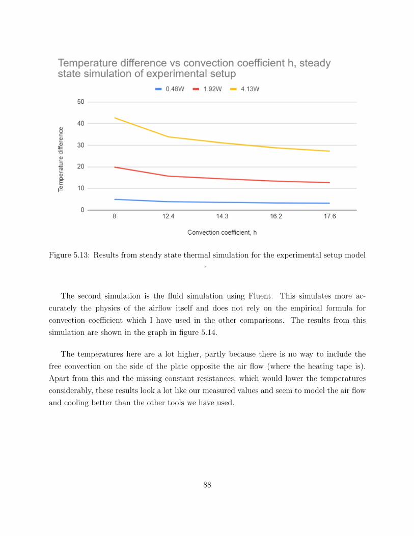
Figure 5.13: Results from steady state thermal simulation for the experimental setup model.
The second simulation is the fluid simulation using Fluent. This simulates more ac-
curately the physics of the airflow itself and does not rely on the empirical formula for
convection coefficient which I have used in the other comparisons. The results from this
simulation are shown in the graph in figure 5.14.
The temperatures here are a lot higher, partly because there is no way to include the
free convection on the side of the plate opposite the air flow (where the heating tape is).
Apart from this and the missing constant resistances, which would lower the temperatures
considerably, these results look a lot like our measured values and seem to model the air flow
and cooling better than the other tools we have used.
88

Figure 5.14: Results from fluid air flow simulation for the experimental setup model.
We have now seen how the methods we have used for predicting the thermal properties of
the tracking layers compares to measurements from a simple air cooling experiment. These
results will be discussed in broader terms in the last chapter.
89

90

Chapter 6
Conclusions/summary
In this last part, the discussions and points that have been made throughout the different
chapters will be repeated and summed up. This is divided into two parts, the mechanical
design part and the thermal properties and cooling part, as these are quite different.
6.1 Mechanical support and air cooling design
As many considerations and limitations as possible has been included in the designs presented
here. Some of the things that have not been considered were not explicitly stated during the
design process and has therefore not been the main priority, like the amount of material in
the design. Also, parts of the pCT have changed during this time and the designs have not
necessarily been flexible enough to change accordingly.
The designs made by A. van der Brink are flexible to new adjustments and are therefore
the current designs for the pCT and cooling test setup. The design processes described here
has been collaborative and my air cooling designs have been a part of making the design
currently in use. Also, my mechanical support design has its own advantages and is useful
for these reasons.
In a design process like this one is made aware of the designs’ flaws and what they lack
and this has in turn been a way to discover new limitations and trade-offs that have to be
made. One does not necessarily have the bigger picture of a project like the pCT from the
start, and this trial and error is essential to the process as the project is changing all the
time.
91
6.2 Cooling of carbon sheets and experimental mea-
surements
To sum up the work in these two chapters:
• Calculation of the effect of water and air cooling on a simplified model of a carbon
sheet and later for a similar aluminium sheet, the cooling test setup from Utrecht.
• Simulation of these same conditions with both a steady state thermal simulation and
a fluid simulation to check the calculations. Some more realistic conditions are im-
plemented for comparison, with the right water and air temperatures and heat load
distribution similar to the 9-chip ALPIDE strings, to compare to the simpler model.
• Assembly of a small test setup with a vent/slit for air cooling and an aluminium plate
with a heating tape. The temperature of the plate was measured to see the effect of
the air cooling.
• Calculation and simulation of the effect of air cooling on my test setup model for
comparing to the results of the measurements.
6.2.1 Calculations
The calculations showed us, first of all, that there would be a need for air cooling of the
tracking layers. This was the purpose of the first heat conduction calculation and it showed
clearly that in a worst case scenario, with all the ALPIDEs generating maximum heat, the
temperature would be too high for optimal operation of the pCT. The alternative ways to
lower the temperature were if we could use carbon sheets that were thicker and/or ones
that had much higher thermal conductivity. Since we want the tracking layers to affect the
particles as little as possible, thicker carbon sheets are not an option and higher thermal
conductivity is not available due to our budget and the small quantity we need.
The next set of calculations was based on the thermal resistances of the different cooling
mechanisms, most importantly air cooling. The only thing not considered here was the
constant resistance from mechanical coupling, glue, flex cables etc. Here we showed that if
we achieve a convection coefficient of 20 Wm2 K
, which corresponds to a laminar air flow with
3.6ms
air speed, that would lower the temperature difference sufficiently.
92

6.2.2 Simulations
Simulating the conditions that we used in the calculations, both in a steady state simulation
and a fluid simulation, confirmed that the calculated values seem reasonable. The weakest
link would then be our model and how it differs from the real-life system. For the next set
of simulations, the water cooling temperature was lower than the temperature of the air, as
low as we can do without condensation. Then, the heat distribution area was changed to
resemble the 9-chip strings of ALPIDEs. Both of these changes resulted in slightly lower
temperature.
The last factors that make these models differ from a real system are the properties of the
air flow and the constant resistances. These are hard to simulate, since they are depending on
a lot of mechanical coupling of parts and simulating a very complex system. Therefore, the
best thing to do when investigating this further is to get some experimental measurements
compare this to the theoretical models.
6.2.3 Experiment
We would have liked to set up the cooling test model made in Utrecht with water cooling
and the proper air cooling design, but unfortunately this was not possible to do within
the time frame of this thesis. Because of this, we decided to use a simpler air cooling test
setup without water cooling. The results from these measurements shows that there is a
significant cooling effect from the air flow, though it is quite turbulent so our estimated
convection coefficient might not be the best approximation for this case. The results from
this experiment have been compared to the calculations and simulations, to see how our
models hold up when compared to experimental measurements.
When using the power drawn by the heating tape as the generated heat, like we did
for the ALPIDEs in the tracking layer model, we saw that the temperatures were higher in
the calculations and simulations than what we had measured. This means that the contact
resistances that we have not included in our model, e.g. between the heating tape and
the aluminium plate and between the aluminium plate and the cardboard, has a significant
impact on the temperature. By adding a non-specified thermal resistance as a substitute for
the constant resistance from e.g. contact resistance, I brought the maximum (free convection)
93

temperature down to my measured values. The slope of the temperature from no air flow to
the 6V fan speed is wrong, which means that value for free convection and/or the empirical
formula calculating the forced convection is wrong in this case.
When simulating these same conditions, the results from the steady state simulations are
similar to our calculated values. The absolute temperature difference is higher because we
have not considered the additional resistances in the simulations. For the fluid simulations
on the other hand, the slopes of the graphs are very similar to the measured results, except
that it is missing a large contribution of constant thermal resistance from various sources.
The fluid simulations made for a much better model than the calculations in this case.
When modeling the carbon layers in chapter 4, we had a large contribution from the water
cooling as the constant temperature boundary conditions. This is easier to anticipate the
effect from than the air flow. In that case, the fluid simulations, steady state simulations and
calculations gave similar results. When modelling the experimental setup, the temperature
difference is relying mostly on the air cooling convection and the simple calculation does not
hold up as well.
These experimental results and corresponding simulations makes me confident that my
results from the calculations and simulations of the tracking layer is a good first estimate
for the temperature difference and distribution. While we do not know the exact values due
to the uncertainties that have been mentioned, we have an idea about the general trends
that these cooling mechanisms will follow. I think that the water and air cooling that is
planned for the tracking layers will be more than sufficient for the optimal operation of the
tracking system for the pCT, even when the ALPIDEs are producing as much heat as they
possibly can. Comparing this experiment to the simulations on the tracking layer model, it
seems like we have considered an absolutely worst case scenario and that the temperatures
will be lower than expected, rather than higher. Concluding anything more certainly than
this would require further testing with a more advanced model that is similar to the real
tracking layers.
6.3 Looking forward
My designs will be useful in the future development of the pCT, and can be changed to fit
further changes if needed. The model I have made is a good estimate for the general trends
94

of the cooling effects, but it is still lacking the constant thermal resistance. The next step
would be to continue testing to figure out the specifics of the air cooling system and the
actual effect of the water cooling. With a proper aluminium replica of the tracking layers,
a more sophisticated experiment and the air cooling design and water cooling in place, we
would get results that are close to the real prototype.
There are also a few things that has been mentioned, which will be important subjects to
investigate further. The fluid dynamics and mechanical properties of the air cooling system
includes air volume flow and pressure loss in ducts, which I have not looked at. The frictional
force from the air flow onto the fragile carbon sheets has been calculated but the impact
of this and the amount of shear stress that the carrier sheets can withstand has not been
looked into. The noise and vibrational frequency of a fan in relation to its volume flow has
also been calculated. This relation and the resonant frequencies of the carbon sheets are an
important subject for further research.
95

96

List of Acronyms and Abbreviations
ALPIDE Alice pixel detector.
CAD computer aided design.
CGE Cobalt Grey equivalent.
CT computed tomography.
DTC digital tracking calorimeter.
IMRT intensity modulated radiotherapy.
IR infrared.
linac linear particle accelerator.
MLC multileaf collimator.
pCT proton computed tomography.
PTV planning target volume.
97

Bibliography
[1] Depth dose curves.
URL: https://www.researchgate.net/figure/Depth-dose-curves-for-radiotherapy-Dose-
distributions-as-a-function-of-depth-in-water fig1 330932948.
[2] Utrecht University A. van der Brink. Private communication.
[3] Kil et al. Proton therapy versus photon radiation therapy for the management of a
recurrent desmoid tumor of the right flank: a case report.
URL: https://www.researchgate.net/figure/Dose-volume-histogram-DVH-data-for-the-
proton-plan-delivered-and-the-corresponding fig4 232703794.
[4] Piersimoni P et. al. A high-granularity digital tracking calorimeter optimized for proton
ct. Front Phys, 8, 2020. doi: https://doi.org/10.3389/fphy.2020.568243.
[5] St. Petersburg University Grigori Fiofilov. Private communication.
[6] Particle Therapy Co-Operative Group. facilities in operation.
URL: https://www.ptcog.ch/index.php/facilities-in-operation.
[7] Komatsu T. Nishiyama S, Yoda K. Reirradiation of spinal metastases using an add-
on double-focus micro multileaf collimator and a three partial-arc conformal avoidance
technique with optimized beam weights: a planning study. J. Diagn. Imaging Ther.,
2015. doi: https://dx.doi.org/10.17229/jdit.2015-0508-017.
[8] Jurges W Nusselt W. The cooling of a flat wall by an airstream (die kuhlung einer
ebenen wand durch einen luftstrom). Gesundh-Ing, 52:641–642, 1922.
[9] Helge Egil Seime Pettersen. A digital tracking calorimeter for proton computed tomog-
raphy, may 2018.
98

[10] Cancer registry of norway. Cancer in norway 2019, (English). pages 2, 82, 2020.
[11] Akos Sudar. Measurement of the temperature distribution inside a calorimeter, decem-
ber 2019.
[12] Suljic M. Alpide: the monolithic active pixel sensor for the alice its upgrade. J Instrum,
11(C11025), 2016. doi: 10.1088/1748-0221/11/11/c11025.
99