mechanics of rubber bearings for seismic and vibration...
TRANSCRIPT
MECHANICS OF RUBBER BEARINGS FOR SEISMIC AND VIBRATION ISOLATION
James M. KellyDimitrios A. Konstantinidis
RED BOX RULES ARE FOR PROOF STAGE ONLY. DELETE BEFORE FINAL PRINTING.
KellyKonstantinidis
MECH
AN
ICS OF RU
BBER BEARIN
GS
FOR SEISM
IC AN
D V
IBRATION
ISOLATIO
N
MECHANICS OF RUBBER BEARINGS FOR SEISMIC AND VIBRATION ISOLATIONJames M. Kelly, University of California, Berkeley, USADimitrios A. Konstantinidis, McMaster University, Hamilton, Canada
Widely used in civil, mechanical and automotive engineering since the early 1980s, multilayer rubber bearings have been used as seismic isolation devices for buildings in highly seismic areas in many countries. Their appeal in these applications comes from their ability to provide a component with high stiffness in one direction and with high fl exibility in one or more orthogonal directions. This combination of vertical stiffness with horizontal fl exibility, achieved by reinforcing the rubber with thin steel shims perpendicular to the vertical load, enables them to be used as seismic and vibration isolators for machinery, buildings and bridges.
Mechanics of Rubber Bearings for Seismic and Vibration Isolation collates the most important information on the mechanics of multilayer rubber bearings. It explores a unique and comprehensive combination of relevant topics, covering all prerequisite fundamental theory and providing a number of closed-form solutions to various boundary value problems as well as a comprehensive historical overview on the use of isolation.
Many of the results presented in the book are new and are essential for a proper understanding of the behavior of these bearings and for the design and analysis of vibration or seismic isolation systems. The advantages afforded by adopting these natural rubber systems is clearly explained to designers and users of this technology, bringing into focus the design and specifi cation of bearings for buildings, bridges and industrial structures.
This comprehensive book:
• includes state of the art, as yet unpublished research along with all required fundamental concepts;
• is authored by world-leading experts with over 40 years of combined experience on seismic isolation and the behavior of multilayer rubber bearings;
• is accompanied by a website at www.wiley.com/go/kelly
The concise approach of Mechanics of Rubber Bearings for Seismic and Vibration Isolation forms an invaluable resource for graduate students and researchers/practitioners in structural and mechanical engineering departments, in particular those working in seismic and vibration isolation.
www.wiley.com/go/kelly

P1: TIX/XYZ P2: ABCJWST069-FM JWST069-Kelly-Style2 July 27, 2011 12:57 Printer Name: Yet to Come
P1: TIX/XYZ P2: ABCJWST069-FM JWST069-Kelly-Style2 July 27, 2011 12:57 Printer Name: Yet to Come
Mechanics of Rubber Bearings forSeismic and Vibration Isolation

P1: TIX/XYZ P2: ABCJWST069-FM JWST069-Kelly-Style2 July 27, 2011 12:57 Printer Name: Yet to Come
P1: TIX/XYZ P2: ABCJWST069-FM JWST069-Kelly-Style2 July 27, 2011 12:57 Printer Name: Yet to Come
Mechanics of RubberBearings for Seismic andVibration Isolation
James M. KellyUniversity of California, Berkeley, USA
Dimitrios A. KonstantinidisMcMaster University, Hamilton, Canada
A John Wiley & Sons, Ltd., Publication

P1: TIX/XYZ P2: ABCJWST069-FM JWST069-Kelly-Style2 July 27, 2011 12:57 Printer Name: Yet to Come
This edition firs published 2011© 2011, John Wiley & Sons, Ltd
Registered officJohn Wiley & Sons Ltd, The Atrium, Southern Gate, Chichester, West Sussex, PO19 8SQ, United Kingdom
For details of our global editorial offices for customer services and for information about how to apply forpermission to reuse the copyright material in this book please see our website at www.wiley.com.
The right of the author to be identifie as the author of this work has been asserted in accordance with theCopyright, Designs and Patents Act 1988.
All rights reserved. No part of this publication may be reproduced, stored in a retrieval system, ortransmitted, in any form or by any means, electronic, mechanical, photocopying, recording or otherwise,except as permitted by the UK Copyright, Designs and Patents Act 1988, without the prior permission of thepublisher.
Wiley also publishes its books in a variety of electronic formats. Some content that appears in print may notbe available in electronic books.
Designations used by companies to distinguish their products are often claimed as trademarks. All brandnames and product names used in this book are trade names, service marks, trademarks or registeredtrademarks of their respective owners. The publisher is not associated with any product or vendormentioned in this book. This publication is designed to provide accurate and authoritative information inregard to the subject matter covered. It is sold on the understanding that the publisher is not engaged inrendering professional services. If professional advice or other expert assistance is required, the services of acompetent professional should be sought.
Library of Congress Cataloging-in-Publication Data
Kelly, James M.Mechanics of rubber bearings for seismic and vibration isolation / James M. Kelly,
Dimitrios A. Konstantinidis.p. cm.
Includes bibliographical references and index.ISBN 978-1-119-99401-5 (hardback)
1. Seismic waves – Damping. 2. Vibration. 3. Rubber bearings. I. Konstantinidis, Dimitrios. II. Title.TJ1073.R8K45 2011620.3′7–dc23 2011013205
A catalogue record for this book is available from the British Library.
Print ISBN: 9781119994015ePDF ISBN: 9781119971887oBook ISBN: 9781119971870ePub ISBN: 9781119972808Mobi ISBN: 9781119972815
Set in 10/12.5pt Palatino by Aptara Inc., New Delhi, India.
P1: TIX/XYZ P2: ABCJWST069-FM JWST069-Kelly-Style2 July 27, 2011 12:57 Printer Name: Yet to Come
Contents
About the Authors ix
Preface xiii
1 History of Multilayer Rubber Bearings 1
2 Behavior of Multilayer Rubber Bearings under Compression 192.1 Introduction 192.2 Pure Compression of Bearing Pads with Incompressible Rubber 19
2.2.1 Infinit Strip Pad 242.2.2 Circular Pad 252.2.3 Rectangular Pad (with Transition to Square or Strip) 262.2.4 Annular Pad 27
2.3 Shear Stresses Produced by Compression 302.4 Pure Compression of Single Pads with Compressible Rubber 33
2.4.1 Infinit Strip Pad 332.4.2 Circular Pad 362.4.3 Rectangular Pad 392.4.4 Annular Pad 40
3 Behavior of Multilayer Rubber Bearings under Bending 453.1 Bending Stiffness of Single Pad with Incompressible Rubber 45
3.1.1 Infinit Strip Pad 473.1.2 Circular Pad 483.1.3 Rectangular Pad 493.1.4 Annular Pad 51
3.2 Bending Stiffness of Single Pads with Compressible Rubber 523.2.1 Infinit Strip Pad 523.2.2 Circular Pad 543.2.3 Rectangular Pad 573.2.4 Annular Pad 58
P1: TIX/XYZ P2: ABCJWST069-FM JWST069-Kelly-Style2 July 27, 2011 12:57 Printer Name: Yet to Come
vi Contents
4 Steel Stress in Multilayer Rubber Bearings under Compressionand Bending 634.1 Review of the Compression and Bending of a Pad 644.2 Steel Stresses in Circular Bearings with Incompressible Rubber 65
4.2.1 Stress Function Solution for Pure Compression 684.2.2 Stress Function Solution for Pure Bending 71
4.3 Steel Stresses in Circular Bearings with Compressible Rubber 734.3.1 Stress Function Solution for Pure Compression 734.3.2 Stress Function Solution for Pure Bending 76
4.4 Yielding of Steel Shims under Compression 784.4.1 Yielding of Steel Shims for the Case of Incompressible Rubber 784.4.2 Yielding of Steel Shims for the Case of Compressible Rubber 79
5 Buckling Behavior of Multilayer Rubber Isolators 835.1 Stability Analysis of Bearings 835.2 Stability Analysis of Annular Bearings 905.3 Influenc of Vertical Load on Horizontal Stiffness 915.4 Downward Displacement of the Top of a Bearing 955.5 A Simple Mechanical Model for Bearing Buckling 100
5.5.1 Postbuckling Behavior 1045.5.2 Influenc of Compressive Load on Bearing Damping Properties 106
5.6 Rollout Stability 1085.7 Effect of Rubber Compressibility on Buckling 110
6 Buckling of Multilayer Rubber Isolators in Tension 1136.1 Introduction 1136.2 Influenc of a Tensile Vertical Load on the Horizontal Stiffness 1156.3 Vertical Displacement under Lateral Load 1176.4 Numerical Modelling of Buckling in Tension 120
6.4.1 Modelling Details 1206.4.2 Critical Buckling Load in Compression and Tension 122
7 Influenc of Plate Flexibility on the Buckling Load of MultilayerRubber Isolators 1297.1 Introduction 1297.2 Shearing Deformations of Short Beams 1307.3 Buckling of Short Beams with Warping Included 1397.4 Buckling Analysis for Bearing 1467.5 Computation of Buckling Loads 153
8 Frictional Restraint on Unbonded Rubber Pads 1598.1 Introduction 1598.2 Compression of Long Strip Pad with Frictional Restraint 1608.3 The Effect of Surface Slip on the Vertical Stiffness of an Infinit Strip Pad 1638.4 The Effect of Surface Slip on the Vertical Stiffness of a Circular Pad 169
P1: TIX/XYZ P2: ABCJWST069-FM JWST069-Kelly-Style2 July 27, 2011 12:57 Printer Name: Yet to Come
Contents vii
9 Effect of Friction on Unbonded Rubber Bearings 1779.1 Introduction 1789.2 Bearing Designs and Rubber Properties 1809.3 Ultimate Displacement of Unbonded Bearings 1809.4 Vertical Stiffness of Unbonded Rubber Bearings with Slip on their
Top and Bottom Supports 184
Appendix: Elastic Connection Device for One or More Degrees of Freedom 193
References 209
Photograph Credits 213
Author Index 215
Subject Index 217

P1: TIX/XYZ P2: ABCJWST069-FM JWST069-Kelly-Style2 July 27, 2011 12:57 Printer Name: Yet to Come
P1: TIX/XYZ P2: ABCJWST069-ATA JWST069-Kelly-Style2 July 15, 2011 14:5 Printer Name: Yet to Come
About the Authors
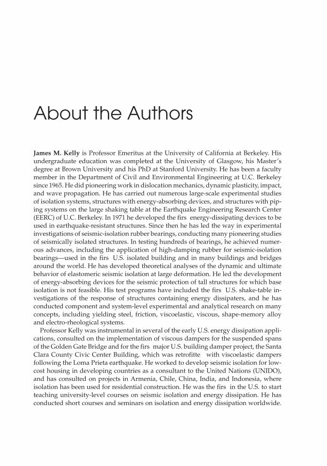
James M. Kelly is Professor Emeritus at the University of California at Berkeley. Hisundergraduate education was completed at the University of Glasgow, his Master’sdegree at Brown University and his PhD at Stanford University. He has been a facultymember in the Department of Civil and Environmental Engineering at U.C. Berkeleysince 1965. He did pioneering work in dislocation mechanics, dynamic plasticity, impact,and wave propagation. He has carried out numerous large-scale experimental studiesof isolation systems, structures with energy-absorbing devices, and structures with pip-ing systems on the large shaking table at the Earthquake Engineering Research Center(EERC) of U.C. Berkeley. In 1971 he developed the firs energy-dissipating devices to beused in earthquake-resistant structures. Since then he has led the way in experimentalinvestigations of seismic-isolation rubber bearings, conducting many pioneering studiesof seismically isolated structures. In testing hundreds of bearings, he achieved numer-ous advances, including the application of high-damping rubber for seismic-isolationbearings—used in the firs U.S. isolated building and in many buildings and bridgesaround the world. He has developed theoretical analyses of the dynamic and ultimatebehavior of elastomeric seismic isolation at large deformation. He led the developmentof energy-absorbing devices for the seismic protection of tall structures for which baseisolation is not feasible. His test programs have included the firs U.S. shake-table in-vestigations of the response of structures containing energy dissipaters, and he hasconducted component and system-level experimental and analytical research on manyconcepts, including yielding steel, friction, viscoelastic, viscous, shape-memory alloyand electro-rheological systems.
Professor Kelly was instrumental in several of the early U.S. energy dissipation appli-cations, consulted on the implementation of viscous dampers for the suspended spansof the Golden Gate Bridge and for the firs major U.S. building damper project, the SantaClara County Civic Center Building, which was retrofitte with viscoelastic dampersfollowing the Loma Prieta earthquake. He worked to develop seismic isolation for low-cost housing in developing countries as a consultant to the United Nations (UNIDO),and has consulted on projects in Armenia, Chile, China, India, and Indonesia, whereisolation has been used for residential construction. He was the firs in the U.S. to startteaching university-level courses on seismic isolation and energy dissipation. He hasconducted short courses and seminars on isolation and energy dissipation worldwide.
P1: TIX/XYZ P2: ABCJWST069-ATA JWST069-Kelly-Style2 July 15, 2011 14:5 Printer Name: Yet to Come
x About the Authors
His work, which formed the basis for significan advances in the analysis and designof seismic isolation and energy-dissipation systems, is the foundation for many of thebase-isolation design codes used today, including UBC, IBC, and CBC. Base isolationhas been used for seismic retrofi of major buildings in the U.S., including importanthistoric structures such as the city halls of Salt Lake City, Oakland, San Francisco, LosAngeles, and the Hearst Memorial Mining Building in Berkeley, on all of which he wasa peer reviewer.
Professor Kelly, well recognized as an outstanding teacher and lecturer, has directedover thirty doctoral students in their PhD thesis research who have gone on to becomenoted practitioners, university professors, and researchers worldwide. Many FulbrightVisiting Scholars have come to Berkeley to work with him. In 1996 he published thesecond edition of his book based on his many years of research and testing at EERC(Earthquake-resistant Design with Rubber, 2nd edn Springer-Verlag). In 1999 he publishedwith Dr Farzad Naeim a textbook on the design of seismic isolated buildings (Design ofSeismic Isolated Structures, John Wiley). He has published over 360 papers over the courseof his career.
Dimitrios A. Konstantinidis is an Assistant Professor at McMaster University. Hereceived his Bachelor’s (1999), Master’s (2001), and PhD (2008) degrees from the Depart-ment of Civil and Environmental Engineering at U.C. Berkeley. His research interestsand experience lie in the fiel of engineering mechanics and earthquake engineeringwith a primary emphasis on seismic isolation, energy dissipation devices, rocking struc-tures, response and protection of building equipment and contents, and structural healthmonitoring.
As a masters student he became interested in the study of rocking structures andconducted research that led to the co-development, with Professor Nicos Makris, of therocking spectrum—a concept analogous to the response spectrum for the single-degree-of-freedom oscillator. He has investigated the seismic response of multi-drum columns,such as those found in ancient temples in Greece, Western Turkey, and Southern Italy,and proposed recommendations against accepted, but unconservative, standard practicein the restoration world. In the earlier stages of his doctoral work, as part of a multi-disciplinary effort to assess the seismic vulnerability of biological research facilities, heinvestigated the seismic response of freestanding and anchored laboratory equipment,which included an extensive experimental program of shaking table tests of full-scaleprototypes and quarter-scale models of equipment. In the later stages of his doctoralwork, he begun working with Professor James M. Kelly. He has studied the effect ofthe isolation type on the response of internal equipment in a base-isolated structure.He has conducted research on the seismic response of bridge bearings which are tra-ditionally used to accommodate various non-seismic translations and rotations of thebridge deck. These included steel-reinforced rubber bearings, steel-reinforced rubber bearingswith Teflo sliding disks, and woven-Teflo spherical bearings. The work included seismic-demand-level dynamic tests at U.C. San Diego and U.C. Berkeley, as well analyticalinvestigations and nonlinear finit element analyses utilizing adaptive remeshing tech-niques to study the behavior of bonded and unbonded rubber bearings under differentloading actions. The finding of the study are being used by Caltrans to develop a new
P1: TIX/XYZ P2: ABCJWST069-ATA JWST069-Kelly-Style2 July 15, 2011 14:5 Printer Name: Yet to Come
About the Authors xi
Memo to Designers guideline and support the development of LRFD-based analysis anddesign procedures for bridge bearings and seismic isolators. The excellent seismic be-havior of rubber bridge bearings, which cost less than a tenth of what rubber seismicisolations cost, has prompted him and Professor Kelly to actively promote the use ofthese bearing as a low-cost alternative for seismic isolation in developing countries,where the cost of conventional isolators is prohibitive.
He has conducted postdoctoral research at U.C. Berkley focusing on the developmentof a health monitoring scheme for viscous flui dampers in bridges using wireless andwired communication. The study involved indoor and outdoor experiments on instru-mented flui dampers. The monitoring system that was developed is being assessed byCaltrans for deployment on testbed bridges.
Before joining the civil engineering faculty at McMaster University in 2011, he wasPostdoctoral Fellow at the Lawrence Berkeley National Laboratory, University of Cali-fornia. His work there concentrated on the base isolation of nuclear power plants andon the evaluation of the U.S. Nuclear Regulatory Commission’s current regulations andguidance for large, conventional Light-water Reactor (LWR) power plants to a newgeneration of small modular reactor (SMR) plants.
Professor Konstantinidis is a member of various professional societies and a reviewerin technical journals, including Earthquake Engineering and Structural Dynamics and Jour-nal of Earthquake Engineering. He has authored 30 publications in refereed journals, inconference proceedings and as technical reports.

P1: TIX/XYZ P2: ABCJWST069-ATA JWST069-Kelly-Style2 July 15, 2011 14:5 Printer Name: Yet to Come
P1: TIX/XYZ P2: ABCJWST069-Preface JWST069-Kelly-Style2 July 20, 2011 10:23 Printer Name: Yet to Come
Preface
The multilayer rubber bearing is an apparently simple device that is used in a widevariety of industries that include civil, mechanical and automotive engineering. It is soubiquitous that it may be difficul to believe that it is a relatively recent development,having been used for only about fift years. The idea of reinforcing rubber blocks bythin steel plates was firs proposed by the famous French engineer Eugene Freyssinet(1879–1962). He recognized that the vertical capacity of a rubber pad was inverselyproportional to its thickness, while its horizontal flexibilit was directly proportional toit. He is best known for the development of prestressed concrete and for the discovery ofcreep in concrete. It is possible that his invention of the reinforced rubber pad was drivenby the need to accommodate the shrinkage of the deck due to creep and prestress load,while sustaining the weight of a prestressed bridge deck. He obtained a French patentin 1954 for his invention, and within a few years the concept was adopted worldwideand led to the extraordinary variety of applications in which multilayer rubber bearingsare used today.
These reinforced rubber bearings in their various forms are a source of fascinatingproblems in solid mechanics. It is the combination of vertical stiffness and horizontalflexibilit , achieved by reinforcing the rubber by thin steel plates perpendicular to thevertical load, that enables them to be used in many applications, including the seismicprotection of buildings and bridges and the vibration isolation of buildings and ma-chinery. The horizontal, vertical, and bending stiffnesses are important to the designof bearings for these applications and for predicting the buckling load, the interactionbetween vertical load and horizontal stiffness, and the dynamic response of structuresand equipment mounted on the bearings.
We will cover the theory for vertical stiffness in Chapter 2 and for bending stiffnessin Chapter 3. Some of the results in these two chapters are new. The results of Chap-ters 2 and 3 are used to predict the stresses in the steel reinforcing plates in Chapter 4.The analysis used to calculate these stresses is new to this text and was only recentlydeveloped by the authors. Also new and original to this text is the development of atheory for these stresses when the effect of the bulk compressibility of the rubber isincluded, which is necessary for seismic isolation bearings, but usually not for vibra-tion isolation bearings. In Chapter 5 we study the stability of these bearings, showing
P1: TIX/XYZ P2: ABCJWST069-Preface JWST069-Kelly-Style2 July 20, 2011 10:23 Printer Name: Yet to Come
xiv Preface
how to estimate buckling loads and the interaction between vertical load and horizontalstiffness as well as a new way to calculate the effect of horizontal displacement on thevertical stiffness. One unexpected aspect of these bearings is that they can buckle intension, and this is covered in Chapter 6. Chapter 7 is concerned with the influencof the flexibilit of the reinforcing plates on the buckling load. This could be impor-tant in efforts to reduce the weight of bearings in the possible application to low-costhousing. Chapters 8 and 9 present some recent research work by the authors on themechanics of bearings that are not bonded to their supports, but are held in place byfriction. This research includes some experimental work on bearings of this type used asbridge bearings.
The original work on the mechanics of rubber bearings was done at the MalaysianRubber Producers Research Association (MRPRA, now the Tun Abdul Razak ResearchCentre) in the United Kingdom in the 1960s under the leadership of Dr A.G. Thomas andDr P.B. Lindley and applied firs to bridge bearings and then to the vibration isolationof residences, hospitals and hotels in the United Kingdom.
The firs building to be isolated from low-frequency ground-borne vibration usingnatural rubber was an apartment block built in 1966 directly above a station ofthe London Underground. Many such projects have been completed in the UnitedKingdom using natural rubber isolators, including a low-cost public housing complexadjacent to two eight-track railway lines that carry 24-hour traffic Several hotelshave been completed using this technology, and a number of hospitals have beenbuilt with this approach. More recently, vibration isolation has been applied toconcert halls.
Some time later MRPRA suggested the use of bearings for the protection of buildingsagainst earthquakes. Dr C.J. Derham, of MRPRA, approached Professor J.M. Kelly andasked him if he was interested in conducting shaking table tests at the Earthquake Sim-ulator Laboratory at the Earthquake Engineering Research Center (EERC), Universityof California at Berkeley, to see to what extent natural rubber bearings could be usedto protect buildings from earthquakes. Very quickly they conducted such a test usinga 20-ton model and handmade isolators. The results from these early tests were verypromising and led to the firs base-isolated building in the United States, also the firsbuilding in the world to use isolation bearings made from high-damping natural rubberdeveloped for this project by MRPRA.
The mathematical complexity in the text varies in different parts of the book, depend-ing on which aspects of the bearings are being studied, but the reader should be assuredthat no more complicated mathematics than absolutely necessary to address the problemat hand has been used.
This text has been written for structural engineers, acoustic engineers and mechanicalengineers with an interest in applying isolation methods to buildings, bridges andindustrial equipment. If they have a background in structural dynamics and an interestin structural mechanics, they will fin that much of the analysis in the text may beapplied to their work. The text can be used as supplementary reading for graduatecourses and as a introduction to dissertation research.
P1: TIX/XYZ P2: ABCJWST069-Preface JWST069-Kelly-Style2 July 20, 2011 10:23 Printer Name: Yet to Come
Preface xv
It will also be useful to those who are charged with preparing or updating designrules and design guidelines for isolated bridges and buildings. The text is the firs thatattempts to bring together in one place the mechanics of rubber bearings now widelyscattered in many journals and reports.
www.wiley.com/go/kelly
James M. KellyDimitrios A. Konstantinidis
Berkeley, California

P1: TIX/XYZ P2: ABCJWST069-Preface JWST069-Kelly-Style2 July 20, 2011 10:23 Printer Name: Yet to Come
P1: TIX/XYZ P2: ABCJWST069-01 JWST069-Kelly-Style2 July 28, 2011 2:34 Printer Name: Yet to Come
1History of MultilayerRubber Bearings
Multilayer rubber bearings are widely used in civil, mechanical and automotive engi-neering. They have been used since the 1950s as thermal expansion bearings for highwaybridges and as vibration isolation bearings for buildings in severe acoustic environments.Since the early 1980s, they have been used as seismic isolation devices for buildings inhighly seismic areas in many countries. Their appeal in these applications is the abilityto provide a component with high stiffness in one direction and high flexibilit in one ormore orthogonal directions. The idea of using thin steel plates as reinforcement in rub-ber blocks was apparently suggested by the famous French engineer Eugene Freyssinet(1879–1962). He recognized that the vertical capacity of a rubber pad was inversely pro-portional to its thickness, while its horizontal flexibilit was directly proportional to thethickness. He is of course best known for the development of prestressed concrete, butalso for the discovery of creep in concrete. It is possible that his invention of the rein-forced rubber pad was driven by the need to accommodate the shrinkage of the deckdue to creep and the prestress load while sustaining the weight of a prestressed bridgedeck. In any case, he obtained a French patent in 1954 for “Dispositif de liaison elastiquea un ou plusieurs degres de liberte” (translated as “Elastic device of connection to oneor more degrees of freedom”; Freyssinet 1954; the patent, with an English translation, isgiven in the Appendix). It seems from his patent that he envisaged that the constrainton the rubber sheets by the reinforcing steel plates be maintained by friction. However,in practical use a more positive connection was desired, and by 1956 bonding of thinsteel plates to rubber sheets during vulcanization was adopted worldwide and led tothe extraordinary variety of applications in which rubber pads are used today.
This combination of horizontal flexibilit and vertical stiffness, achieved by reinforcingthe rubber by thin steel shims perpendicular to the vertical load, enables them to beused in many applications, including seismic protection of buildings and bridges andvibration isolation of machinery and buildings.
Mechanics of Rubber Bearings for Seismic and Vibration Isolation, First Edition. James M. Kelly and Dimitrios A. Konstantinidis.C© 2011 John Wiley & Sons, Ltd. Published 2011 by John Wiley & Sons, Ltd.
1
P1: TIX/XYZ P2: ABCJWST069-01 JWST069-Kelly-Style2 July 28, 2011 2:34 Printer Name: Yet to Come
2 History of Multilayer Rubber Bearings
The isolation of equipment from vibration via anti-vibration mounts is a well-established technology, and the theory and practice are covered in several books, papers,and reviews; the survey by Snowden (1979) is an example. Although the isolated ma-chine is usually the source of the unwanted vibrations, the procedure can also be used toprotect either a sensitive piece of equipment or an entire building from external sourcesof vibration. The use of vibration isolation for entire buildings originated in the UnitedKingdom and is now well accepted throughout Europe and is beginning to be usedin the United States. Details of this method of building construction can be found inGrootenhuis (1983) and Crockett (1983).
The predominant disturbance to a building by rail traffi is a vertical ground motionwith frequencies ranging from 25 to 50 Hz, depending on the local soil conditions and thesource. To achieve a degree of attenuation that takes the disturbance below the thresholdof perception or below the level that interferes with the operation of delicate equipment(e.g., an electron microscope), rubber bearings are designed to provide a vertical naturalfrequency for the structure about one-third of the lowest frequency of the disturbance.
The firs building to be isolated from low-frequency ground-borne vibration usingnatural rubber was an apartment block built in London in 1966. Known as AlbanyCourt, this building is located directly above the St James’ Park Station of the LondonUnderground. This project was experimental to a certain extent, and the performanceand durability of the isolation system in the years since its construction was monitoredfor several years by the Malaysian Rubber Producers Research Association (MRPRA,now the Tun Abdul Razak Research Centre) in conjunction with Aktins Research andDevelopment (Derham and Waller 1975).
Since then, many projects have been completed in the United Kingdom using naturalrubber isolators. These have included Grafton 16, a low-cost public housing complex thatwas built on a site adjacent to two eight-track railway lines that carry 24-hour traffic Inthis project the isolators produced a vertical frequency of 6.5 Hz to isolate against groundmotion in the 20 Hz range. Several hotels have been completed using this technology, forexample, the Holiday Inn in Swiss Cottage in London. In addition, a number of hospitalshave been built with this approach, which is particularly advantageous when precisiondiagnostic equipment is present.
More recently, vibration isolation has been applied for use in concert halls. In 1990, theGlasgow Royal Concert Hall, which is sited directly above two underground railwaylines, was completed in Glasgow, Scotland. The building has a reinforced concretestructural frame that is supported on 450 natural rubber bearings. In addition to housingthe 2850-seat concert hall, it also contains a conference hall and a number of restaurants.
Another concert hall is the International Convention Centre in Birmingham, England,which was completed in 1991. Home of the City of Birmingham Symphony Orchestra, thebuilding comprises ten conference halls and a 2211-seat concert hall. The entire complexwas built at a cost of £121 million and is supported on 2000 natural rubber bearings toisolate it from noise from a main line railway running in a tunnel near the site.
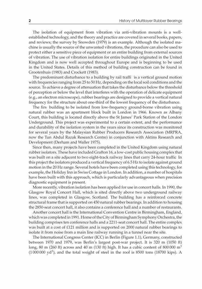
The International Congress Center (ICC) in Berlin (Figure 1.1), Germany, constructedbetween 1970 and 1979, was Berlin’s largest post-war project. It is 320 m (1050 ft)long, 80 m (260 ft) across and 40 m (130 ft) high. It has a cubic content of 800 000 m3
(1 000 000 yd3), and the total weight of steel in the roof is 8500 tons (18700 kips). A
P1: TIX/XYZ P2: ABCJWST069-01 JWST069-Kelly-Style2 July 28, 2011 2:34 Printer Name: Yet to Come
History of Multilayer Rubber Bearings 3
Figure 1.1 The International Congress Center (ICC) in Berlin, Germany. Reproduced fromHans-Georg Weimar, Wikimedia
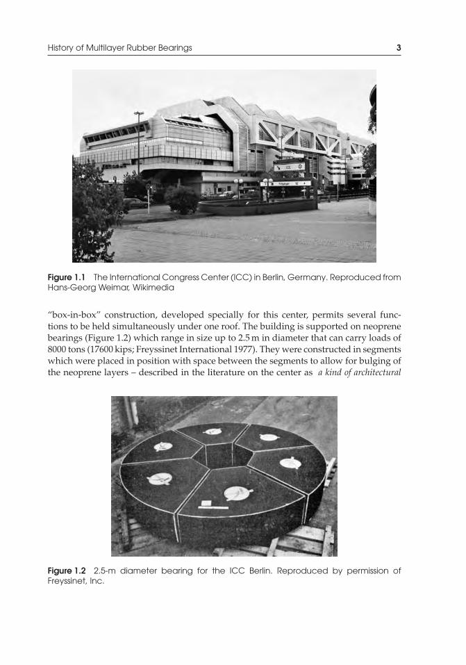
“box-in-box” construction, developed specially for this center, permits several func-tions to be held simultaneously under one roof. The building is supported on neoprenebearings (Figure 1.2) which range in size up to 2.5 m in diameter that can carry loads of8000 tons (17600 kips; Freyssinet International 1977). They were constructed in segmentswhich were placed in position with space between the segments to allow for bulging ofthe neoprene layers – described in the literature on the center as a kind of architectural
Figure 1.2 2.5-m diameter bearing for the ICC Berlin. Reproduced by permission ofFreyssinet, Inc.
P1: TIX/XYZ P2: ABCJWST069-01 JWST069-Kelly-Style2 July 28, 2011 2:34 Printer Name: Yet to Come
4 History of Multilayer Rubber Bearings
shock absorber – and were intended to exclude outside noise and absorb vibrations froman adjacent highway and railway. ICC Berlin has over 80 halls and conference rooms,with seating capacities ranging from 20 to 5000, with a sophisticated information anddirection system. The largest hall (Hall 1) can seat up to 5000 and has the second-largeststage in Europe.
Two recent applications of vibration isolation to concert halls in the United States arethe Benaroya Concert Hall in Seattle, Washington, completed in 1999 and the Walt DisneyConcert Hall in Los Angeles, California, completed in 2003. The firs uses rubber bearingsto mitigate ground-borne noise from trains in a tunnel below the hall. The Walt DisneyConcert Hall is built directly above a loading dock for an immediately adjacent building.The interesting thing about these two buildings is that they are located in highly seismicareas, yet there was no attempt on the part of the structural engineers for either project tocombine both vibration isolation and seismic isolation in the same system. Experimentalresults of tests done at the shake table at the Earthquake Engineering Research Centerof the University of California, Berkeley, many years before the construction of thesetwo concert halls, demonstrated that it was possible to design a rubber bearing systemthat would provide both vibration isolation and seismic protection. In the concert hallprojects, lateral movement of the bearings that support the buildings is prevented by asystem of many vertically located bearings, the additional cost of which is substantialand could have been avoided by appropriate design.
Seismic isolation can also be provided by multilayer rubber bearings that, in thiscase, decouple the building or structure from the horizontal components of the groundmotion through the low horizontal stiffness of the bearings, which give the structure afundamental frequency that is much lower than both its fixed-bas frequency and thepredominant frequencies of the ground motion. The firs dynamic mode of the isolatedstructure involves deformation only in the isolation system, the structure above beingto all intents and purposes rigid. The higher modes that produce deformation in thestructure are orthogonal to the firs mode and, consequently, to the ground motion(Kelly 1997). These higher modes do not participate, so that if there is high energy inthe ground motion at these higher frequencies, this energy cannot be transmitted intothe structure. The isolation system does not absorb the earthquake energy, but ratherdeflect it through the dynamics of the system. This type of isolation system works whenthe system is linear, and even when undamped; however, a certain level of damping isbeneficia to suppress any possible resonance at the isolation frequency. This dampingcan be provided by the rubber compound itself through appropriate compounding. Therubber compounds in common engineering use have an intrinsic energy dissipationequivalent to 2–3% of linear viscous damping, but in compounds referred to as high-damping rubber this can be increased to 10–20% (Naeim and Kelly 1999).
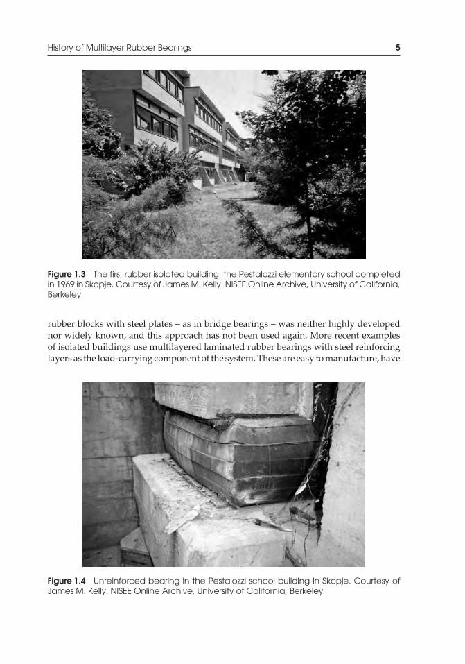
The firs use of rubber for the earthquake protection of a structure was in an elementaryschool, completed in 1969 in Skopje, in the Former Yugoslav Republic of Macedonia (seeFigure 1.3). The building is a three-story concrete structure that rests on large blocks ofnatural rubber (Garevski et al. 1998). Unlike more recently developed rubber bearings,these blocks are completely unreinforced so that the weight of the building causes themto bulge sideways (see Figure 1.4). Because the vertical and horizontal stiffnesses of thesystem are about the same, the building will bounce and rock backwards and forwardsin an earthquake. These bearings were designed when the technology for reinforcing
P1: TIX/XYZ P2: ABCJWST069-01 JWST069-Kelly-Style2 July 28, 2011 2:34 Printer Name: Yet to Come
History of Multilayer Rubber Bearings 5
Figure 1.3 The firs rubber isolated building: the Pestalozzi elementary school completedin 1969 in Skopje. Courtesy of James M. Kelly. NISEE Online Archive, University of California,Berkeley
rubber blocks with steel plates – as in bridge bearings – was neither highly developednor widely known, and this approach has not been used again. More recent examplesof isolated buildings use multilayered laminated rubber bearings with steel reinforcinglayers as the load-carrying component of the system. These are easy to manufacture, have
Figure 1.4 Unreinforced bearing in the Pestalozzi school building in Skopje. Courtesy ofJames M. Kelly. NISEE Online Archive, University of California, Berkeley
P1: TIX/XYZ P2: ABCJWST069-01 JWST069-Kelly-Style2 July 28, 2011 2:34 Printer Name: Yet to Come
6 History of Multilayer Rubber Bearings
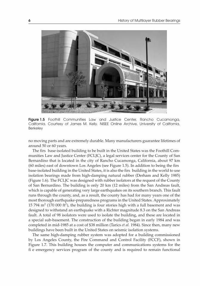
Figure 1.5 Foothill Communities Law and Justice Center, Rancho Cucamonga,California. Courtesy of James M. Kelly. NISEE Online Archive, University of California,Berkeley
no moving parts and are extremely durable. Many manufacturers guarantee lifetimes ofaround 50 or 60 years.
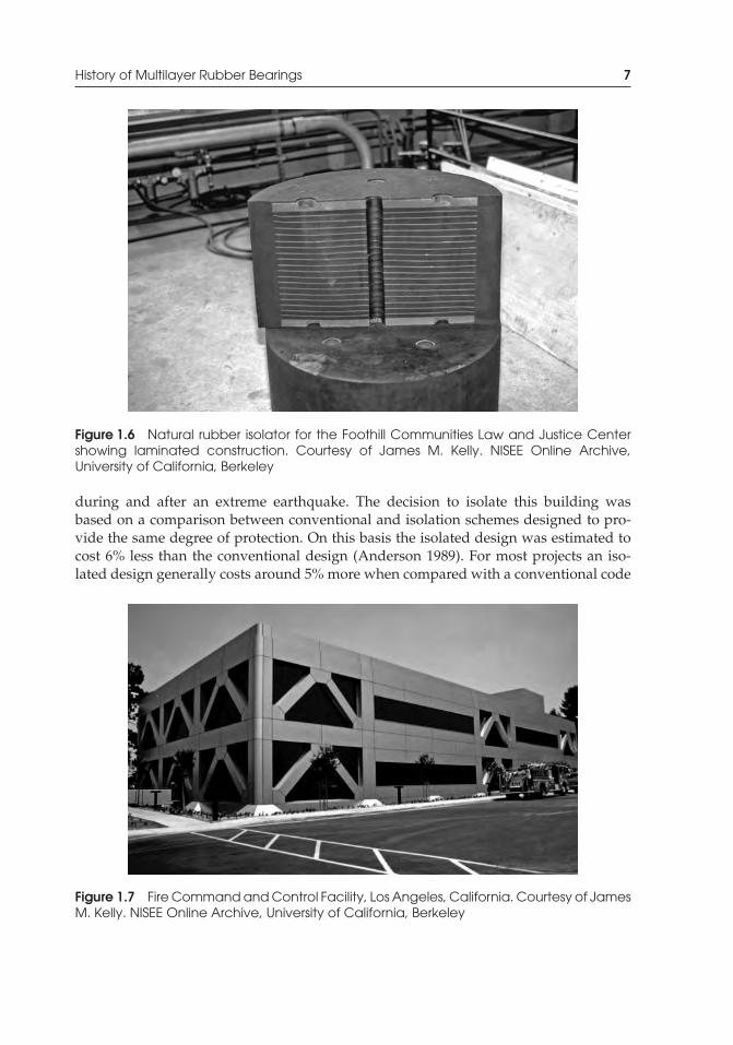
The firs base-isolated building to be built in the United States was the Foothill Com-munities Law and Justice Center (FCLJC), a legal services center for the County of SanBernardino that is located in the city of Rancho Cucamonga, California, about 97 km(60 miles) east of downtown Los Angeles (see Figure 1.5). In addition to being the firsbase-isolated building in the United States, it is also the firs building in the world to useisolation bearings made from high-damping natural rubber (Derham and Kelly 1985)(Figure 1.6). The FCLJC was designed with rubber isolators at the request of the Countyof San Bernardino. The building is only 20 km (12 miles) from the San Andreas fault,which is capable of generating very large earthquakes on its southern branch. This faultruns through the county, and, as a result, the county has had for many years one of themost thorough earthquake-preparedness programs in the United States. Approximately15 794 m2 (170 000 ft2), the building is four stories high with a full basement and wasdesigned to withstand an earthquake with a Richter magnitude 8.3 on the San Andreasfault. A total of 98 isolators were used to isolate the building, and these are located ina special sub-basement. The construction of the building began in early 1984 and wascompleted in mid-1985 at a cost of $38 million (Tarics et al. 1984). Since then, many newbuildings have been built in the United States on seismic isolation systems.
The same high-damping rubber system was adopted for a building commissionedby Los Angeles County, the Fire Command and Control Facility (FCCF), shown inFigure 1.7. This building houses the computer and communications systems for thefi e emergency services program of the county and is required to remain functional
P1: TIX/XYZ P2: ABCJWST069-01 JWST069-Kelly-Style2 July 28, 2011 2:34 Printer Name: Yet to Come
History of Multilayer Rubber Bearings 7
Figure 1.6 Natural rubber isolator for the Foothill Communities Law and Justice Centershowing laminated construction. Courtesy of James M. Kelly. NISEE Online Archive,University of California, Berkeley
during and after an extreme earthquake. The decision to isolate this building wasbased on a comparison between conventional and isolation schemes designed to pro-vide the same degree of protection. On this basis the isolated design was estimated tocost 6% less than the conventional design (Anderson 1989). For most projects an iso-lated design generally costs around 5% more when compared with a conventional code
Figure 1.7 Fire Command and Control Facility, Los Angeles, California. Courtesy of JamesM. Kelly. NISEE Online Archive, University of California, Berkeley

P1: TIX/XYZ P2: ABCJWST069-01 JWST069-Kelly-Style2 July 28, 2011 2:34 Printer Name: Yet to Come
8 History of Multilayer Rubber Bearings
design; however, the design code provides a minimum level of protection against strongground shaking, guaranteeing only that the building will not collapse. It does not protectthe building from structural damage. When equivalent levels of design performance arecompared, an isolated building is always more cost effective. Additionally, these arethe primary costs when contemplating a structural system and do not address the life-cycle costs, which are also more favorable when an isolation system is used as comparedto conventional construction.
A second base-isolated building, also built for the County of Los Angeles, is at thesame location as the FCCF. The Emergency Operations Center (EOC) is a two-storysteel braced-frame structure isolated using 28 high-damping natural rubber bearingsprovided by the Bridgestone Engineered Products Co., Inc.
The most recent example of an isolated emergency center is the two-story Caltrans/CHP Traffi Management Center in Kearny Mesa near San Diego, California (Walterset al. 1995). The superstructure has a steel frame with perimeter concentrically bracedbays. The isolation system, also provided by Bridgestone, consists of 40 high-dampingnatural rubber isolators. The isolators are 60 cm (24 in) in diameter.
The use of seismic isolation for emergency control centers is clearly advantageoussince these buildings contain essential equipment that must remain functional duringand after an earthquake. They are designed to a much higher level of performance thanconventional buildings, and the increased cost for the isolators is easily justified Otherexamples are the San Francisco 911 Center and the Public Safety Building in the city ofBerkeley, California.
Other base-isolated building projects in California include a number of hospitals.The M. L. King Jr–C. R. Drew Diagnostics Trauma Center in Willowbrook, California,is a 13 006 m2 (140 000 ft2), five-stor structure supported on 70 high-dampingnatural rubber bearings and 12 sliding bearings with lead–bronze plates that slide ona stainless steel surface. Built for the County of Los Angeles, the building is locatedwithin 5 km (3 miles) of the Newport–Inglewood fault, which is capable of generat-ing earthquakes with a Richter magnitude of 7.5. The isolators are 100 cm (40 in) indiameter, and at the time of their manufacture were the largest isolation bearings fab-ricated in the United States. Many other hospitals have been built in California sincethen on rubber isolation systems, some with lead–rubber bearings (i.e., multilayeredrubber bearings featuring a cylindrical lead core) and some with high-damping rubberbearings. They include the University of Southern California Teaching hospital, usinglead–rubber bearings, completed in 1991. This hospital, which was instrumented withstrong-motion seismic acceleration instruments was impacted by the 1994 NorthridgeEarthquake and performed remarkably well. The peak ground acceleration in the freefiel (the parking lot) was 0.49g, which was reduced within the building to around0.10–0.11g by the isolation system. The Arrowhead Regional Medical Center, part of theCounty of San Bernardino, was completed in 1998, and the St Johns Medical Center, aprivate hospital in Santa Monica, in 2001. Two hospitals owned by Hoag Presbyterianin Irvine, one a retrofi and one new, were built on high-damping rubber bearings in themid 2000s.
In addition to new buildings, there are a number of very large retrofi projects inCalifornia using base isolation, including the retrofi of the Oakland City Hall and the
P1: TIX/XYZ P2: ABCJWST069-01 JWST069-Kelly-Style2 July 28, 2011 2:34 Printer Name: Yet to Come
History of Multilayer Rubber Bearings 9
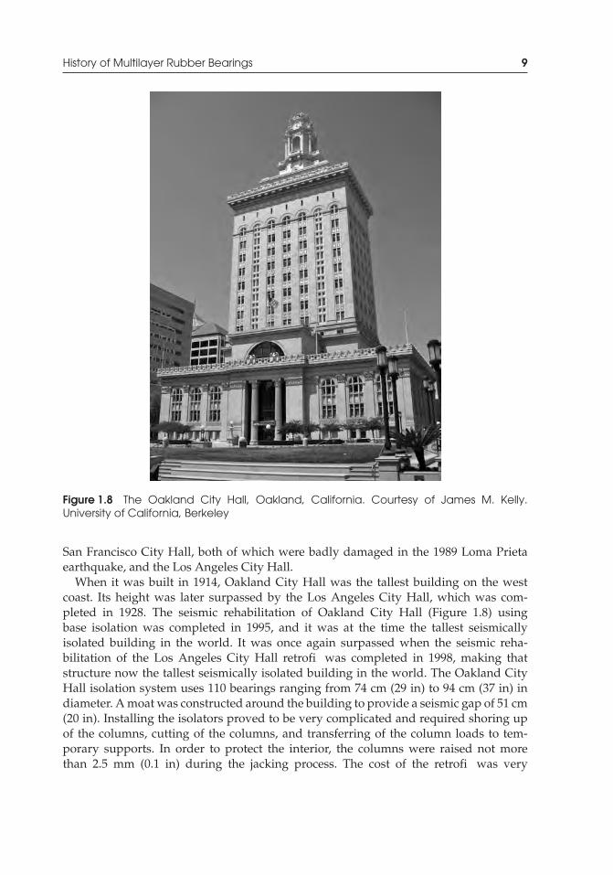
Figure 1.8 The Oakland City Hall, Oakland, California. Courtesy of James M. Kelly.University of California, Berkeley
San Francisco City Hall, both of which were badly damaged in the 1989 Loma Prietaearthquake, and the Los Angeles City Hall.
When it was built in 1914, Oakland City Hall was the tallest building on the westcoast. Its height was later surpassed by the Los Angeles City Hall, which was com-pleted in 1928. The seismic rehabilitation of Oakland City Hall (Figure 1.8) usingbase isolation was completed in 1995, and it was at the time the tallest seismicallyisolated building in the world. It was once again surpassed when the seismic reha-bilitation of the Los Angeles City Hall retrofi was completed in 1998, making thatstructure now the tallest seismically isolated building in the world. The Oakland CityHall isolation system uses 110 bearings ranging from 74 cm (29 in) to 94 cm (37 in) indiameter. A moat was constructed around the building to provide a seismic gap of 51 cm(20 in). Installing the isolators proved to be very complicated and required shoring upof the columns, cutting of the columns, and transferring of the column loads to tem-porary supports. In order to protect the interior, the columns were raised not morethan 2.5 mm (0.1 in) during the jacking process. The cost of the retrofi was very
P1: TIX/XYZ P2: ABCJWST069-01 JWST069-Kelly-Style2 July 28, 2011 2:34 Printer Name: Yet to Come
10 History of Multilayer Rubber Bearings
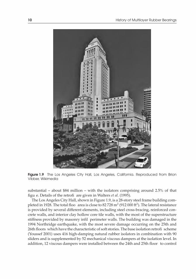
Figure 1.9 The Los Angeles City Hall, Los Angeles, California. Reproduced from BrionVibber, Wikimedia
substantial – about $84 million – with the isolators comprising around 2.5% of thatfigu e. Details of the retrofi are given in Walters et al. (1995).
The Los Angeles City Hall, shown in Figure 1.9, is a 28-story steel frame building com-pleted in 1928. The total floo area is close to 82 728 m2 (912 000 ft2). The lateral resistanceis provided by several different elements, including steel cross-bracing, reinforced con-crete walls, and interior clay hollow core tile walls, with the most of the superstructurestiffness provided by masonry infil perimeter walls. The building was damaged in the1994 Northridge earthquake, with the most severe damage occurring on the 25th and26th floors which have the characteristic of soft stories. The base isolation retrofi scheme(Youssef 2001) uses 416 high-damping natural rubber isolators in combination with 90sliders and is supplemented by 52 mechanical viscous dampers at the isolation level. Inaddition, 12 viscous dampers were installed between the 24th and 25th floor to control
P1: TIX/XYZ P2: ABCJWST069-01 JWST069-Kelly-Style2 July 28, 2011 2:34 Printer Name: Yet to Come
History of Multilayer Rubber Bearings 11
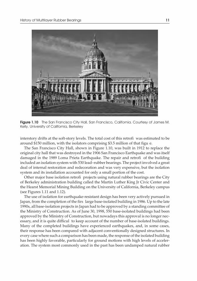
Figure 1.10 The San Francisco City Hall, San Francisco, California. Courtesy of James M.Kelly. University of California, Berkeley
interstory drifts at the soft-story levels. The total cost of this retrofi was estimated to bearound $150 million, with the isolators comprising $3.5 million of that figu e.
The San Francisco City Hall, shown in Figure 1.10, was built in 1912 to replace theoriginal city hall that was destroyed in the 1906 San Francisco Earthquake and was itselfdamaged in the 1989 Loma Prieta Earthquake. The repair and retrofi of the buildingincluded an isolation system with 530 lead–rubber bearings. The project involved a greatdeal of internal restoration and redecoration and was very expensive, but the isolationsystem and its installation accounted for only a small portion of the cost.
Other major base isolation retrofi projects using natural rubber bearings are the Cityof Berkeley administration building called the Martin Luther King Jr Civic Center andthe Hearst Memorial Mining Building on the University of California, Berkeley campus(see Figures 1.11 and 1.12).
The use of isolation for earthquake-resistant design has been very actively pursued inJapan, from the completion of the firs large base-isolated building in 1986. Up to the late1990s, all base-isolation projects in Japan had to be approved by a standing committee ofthe Ministry of Construction. As of June 30, 1998, 550 base-isolated buildings had beenapproved by the Ministry of Construction, but nowadays this approval is no longer nec-essary, and it is quite difficul to keep account of the number of base-isolated buildings.Many of the completed buildings have experienced earthquakes, and, in some cases,their response has been compared with adjacent conventionally designed structures. Inevery case where such a comparison has been made, the response of the isolated buildinghas been highly favorable, particularly for ground motions with high levels of acceler-ation. The system most commonly used in the past has been undamped natural rubber
P1: TIX/XYZ P2: ABCJWST069-01 JWST069-Kelly-Style2 July 28, 2011 2:34 Printer Name: Yet to Come
12 History of Multilayer Rubber Bearings
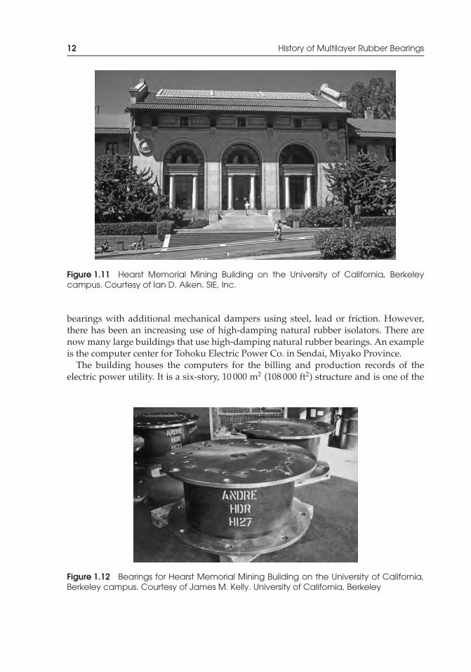
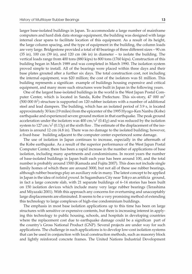
Figure 1.11 Hearst Memorial Mining Building on the University of California, Berkeleycampus. Courtesy of Ian D. Aiken. SIE, Inc.
bearings with additional mechanical dampers using steel, lead or friction. However,there has been an increasing use of high-damping natural rubber isolators. There arenow many large buildings that use high-damping natural rubber bearings. An exampleis the computer center for Tohoku Electric Power Co. in Sendai, Miyako Province.
The building houses the computers for the billing and production records of theelectric power utility. It is a six-story, 10 000 m2 (108 000 ft2) structure and is one of the
Figure 1.12 Bearings for Hearst Memorial Mining Building on the University of California,Berkeley campus. Courtesy of James M. Kelly. University of California, Berkeley
P1: TIX/XYZ P2: ABCJWST069-01 JWST069-Kelly-Style2 July 28, 2011 2:34 Printer Name: Yet to Come
History of Multilayer Rubber Bearings 13
larger base-isolated buildings in Japan. To accommodate a large number of mainframecomputers and hard disk data storage equipment, the building was designed with largeinternal clear spans to facilitate location of this equipment. As a result of its height,the large column spacing, and the type of equipment in the building, the column loadsare very large. Bridgestone provided a total of 40 bearings of three different sizes – 90 cm(35 in), 100 cm (39 in), and 120 cm (46 in) in diameter – to isolate the building. Thevertical loads range from 400 tons (880 kips) to 800 tons (1760 kips). Construction of thisbuilding began in March 1989 and was completed in March 1990. The isolation systemproved simple to install. All of the bearings were placed within three days and theirbase plates grouted after a further six days. The total construction cost, not includingthe internal equipment, was $20 million; the cost of the isolators was $1 million. Thisbuilding represents a significan example of buildings housing expensive and criticalequipment, and many more such structures were built in Japan in the following years.
One of the largest base-isolated buildings in the world is the West Japan Postal Com-puter Center, which is located in Sanda, Kobe Prefecture. This six-story, 47 000 m2
(500 000 ft2) structure is supported on 120 rubber isolators with a number of additionalsteel and lead dampers. The building, which has an isolated period of 3.9 s, is locatedapproximately 30 km (19 miles) from the epicenter of the 1995 Hyogo-Ken Nanbu (Kobe)earthquake and experienced severe ground motion in that earthquake. The peak groundacceleration under the isolators was 400 cm/s2 (0.41g) and was reduced by the isolationsystem to 127 cm/s2 (0.13g) at the sixth floo . The estimate of the displacement of the iso-lators is around 12 cm (4.8 in). There was no damage to the isolated building; however,a fixed-base building adjacent to the computer center experienced some damage.
The use of isolation in Japan continues to increase, especially in the aftermath ofthe Kobe earthquake. As a result of the superior performance of the West Japan PostalComputer Center, there has been a rapid increase in the number of applications of baseisolation, including many apartments and condominiums. In recent years the numberof base-isolated buildings in Japan built each year has been around 100, and the totalnumber is probably around 1500 (Kamada and Fujita 2007). This does not include singlefamily homes of which there are around 3000, but not all of these use rubber bearings,although rubber bearings play an auxiliary role in many. The latest concept to be appliedin Japan is the idea of isolated ground. In Sagamihara City near Tokyo an artificia ground,in fact a large concrete slab, with 21 separate buildings of 6–14 stories has been builton 150 isolation devices which include many very large rubber bearings (Terashimaand Miyazaki 2001). With this approach any concerns for overturning and unacceptablylarge displacements are eliminated. It seems to be a very promising method of extendingthis technology to large complexes of high-rise condominium buildings.
The emphasis in most base isolation applications up to this time has been on largestructures with sensitive or expensive contents, but there is increasing interest in apply-ing this technology to public housing, schools, and hospitals in developing countrieswhere the replacement cost due to earthquake damage could be a significan part ofthe country’s Gross National Product (GNP). Several projects are under way for suchapplications. The challenge in such applications is to develop low-cost isolation systemsthat can be used in conjunction with local construction methods, such as masonry blockand lightly reinforced concrete frames. The United Nations Industrial Development
P1: TIX/XYZ P2: ABCJWST069-01 JWST069-Kelly-Style2 July 28, 2011 2:34 Printer Name: Yet to Come
14 History of Multilayer Rubber Bearings
Organization (UNIDO) partially finance a joint effort between the Malaysian RubberProducers’ Research Association (MRPRA, now the Tun Abdul Razak Research Centre)of the United Kingdom and the Earthquake Engineering Research Center (EERC) of theUniversity of California at Berkeley to research and promote the use of rubber bearingsfor base-isolated buildings in developing countries.
To date, a number of base-isolated demonstration projects have been completed. Inmost cases an identical structure of fixed-bas construction was built adjacent to theisolated building to compare their behavior during earthquakes. There are demonstra-tion projects in Reggio Calabria, Italy; Santiago, Chile; Guangdong Province, China; andPelabuhan Ratu, Indonesia.
One of the demonstration projects completed under this program is a base-isolatedapartment building in the coastal city of Shantou, Guangdong Province, an earthquake-prone area of southern China. Completed in 1994, this building is the firs rubberbase-isolated building in China. This demonstration project involved the constructionof two eight-story housing blocks. Two identical and adjacent buildings were built; onebuilding is of conventional fixed-bas construction, and the other is base-isolated withhigh-damping natural rubber isolators. The design, testing, and manufacture of theisolators was funded by the MRPRA from a grant provided by the UNIDO. The demon-stration project was a joint effort by the MRPRA, the EERC, and Nanyang University,Singapore. Details of this project can be found in Taniwangsa and Kelly (1996).
As part of the UNIDO support, several rubber technologists from a rubbercompany in Shantou went to the MRPRA laboratory and were trained in the manu-facture of rubber isolators. The city of Shantou provided a site, and a factory producingrubber isolators was established in this city. This company has supplied isolators forprojects all over China, many of them large complexes of perhaps 30–40 identical eight-story multi-family housing blocks. It also supplied isolators for buildings in Japan andin Russia.
In 1994 construction of a base-isolated four-story reinforced concrete building in Java,Indonesia, was completed (Figure 1.13). The construction of this demonstration buildingwas part of the same UNIDO-sponsored program to introduce base isolation technologyto developing countries. In order for this new technology to be readily adopted bybuilding officials it was essential that the design and construction of the superstructureof the isolated building did not deviate substantially from common building practiceand building codes used for fixed-bas buildings.
The demonstration building in Indonesia is located in the southern part of WestJava, about 1 km (0.6 miles) southwest of Pelabuhan Ratu. The building is a four-story moment-resisting reinforced concrete structure, accommodating eight low-costapartment units. The building is 7.2 × 18.0 m (24 × 59 ft) in plan, and the height tothe roof above the isolators is 12.8 m (42 ft). The walls that enclose each apartmentunit are made out of unreinforced masonry with special seismic gaps fille with softmortar. A common building practice in Indonesia, this type of seismic gap separatesthe walls from the main structure. This building is supported by 16 high-dampingnatural rubber bearings. The isolation bearings are located at the ground level and areconnected to the superstructure using an innovative recessed end-plate connection, as

P1: TIX/XYZ P2: ABCJWST069-01 JWST069-Kelly-Style2 July 28, 2011 2:34 Printer Name: Yet to Come
History of Multilayer Rubber Bearings 15
Figure 1.13 Demonstration building in Pelabuhan Ratu, West Java, Indonesia. Courtesyof James M. Kelly. University of California, Berkeley
opposed to the more usual bolted connection. This use of a recessed end-plate connectionproved to be cost-effective and very easy to install. The bearings were designed andmanufactured by the MRPRA in the United Kingdom. To achieve overall economy offabrication, installation, and maintenance of the isolation system, two different high-damping natural rubber compounds were used, and a single bearing size was selectedso that only one mold was necessary for the fabrication process. The dynamic propertiesof the bearings were confirme by full-size bearing tests. Details of this project can befound in Taniwangsa and Kelly (1996).
Nuclear power plants are another example of a type of structure for which seismicisolation can be extremely beneficial Nuclear structures are generally very stiff andheavy, thus the benefit of a large-period shift can be obtained easily without resortingto long-period isolation systems. Also, as will be shown later, it is much easier to designstable isolators for heavier loads than light loads. Because the response of a base-isolatedstructure is dominated by the lowest mode, i.e., the structure moves in an approximatelyrigid-body manner, the stress analysis of the structure is greatly simplified A substantiallevel of design effort in nuclear facilities is devoted to the dynamic analysis of equipmentand piping systems. The conventional design involves computing floo spectra for each
P1: TIX/XYZ P2: ABCJWST069-01 JWST069-Kelly-Style2 July 28, 2011 2:34 Printer Name: Yet to Come
16 History of Multilayer Rubber Bearings
level, and, in some cases, multiple input spectra when piping systems or equipmentitems are attached at more than one level, and then broadening these spectra to accountfor uncertainties in the analysis.
In an isolated structure, however, because the dominant mode is a rigid-body modewith all the deformation concentrated at the isolation level, all parts of the buildingmove in the same way at the low isolation frequency. The response uncertainties arereduced, multiple input spectra are not needed, and the peaks in all the floo spectraare at the low frequency of the isolation system, which is generally much lower thanequipment or piping frequencies (Yang et al. 2010).
Thus using an isolation system allows a high degree of standardization, with equip-ment qualificatio processes simplifie through reduced seismic levels. A further benefiis that if the regulatory environment changes during the life of the plant, mandating anupgrade of the seismic input, the response of the equipment may not be greatly affected.If there is more than a negligible increase in the design forces at the isolation frequency,it is a relatively simple matter to reduce the overall stiffness of the isolation system andmaintain the original equipment standards.
Because nuclear plants are a natural application of base isolation technology, it is nosurprise that one of the earliest applications of the technology was a nuclear facility.Completed in 1980, the Koeberg Power Plant in South Africa was both the firs base-isolated nuclear power plant and one of the firs base-isolated buildings (Renault et al.1979; Plichon et al. 1980). The power plant, designed by Electricite de France and builtby Spie Batignolles, has two 900 MWe standardized units, which had been qualifie forseismic inputs up to 0.2g. The nuclear island is constructed on 1829 aseismic bearingson concrete pedestals. Standard bridge bearings were used, consisting of multilayerneoprene bearings topped by bronze slip plates which slide on stainless steel platesattached to the underside of the upper base mat. These bearings were designed in theearly 1970s when the technology of rubber isolators was such that the maximum lateraldisplacements were quite small, of the order of 5 cm (2 in). If the bearings reach thisdisplacement, the sliding plates are expected to slip and provide further displacement.Because of subsequent developments in isolator design and manufacturing, it is unlikelythat this design will be used again; in fact, a subsequent isolated nuclear power plantbuilding by Electricite de France at Cruas uses only rubber pads.
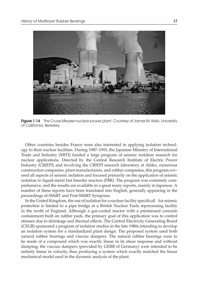
The Cruas Nuclear Power Plant (Postollec 1982), shown in Figure 1.14, comprisedfour 900 MWe PWR units supported on 3600 neoprene isolators, was constructed on anisolated nuclear island. The designers decided to isolate Cruas because the seismicity ofthe site exceeded that for which all previous examples of this standardized plant hadbeen designed. The buildings and equipment of the standardized plant were designedfor the basic EDF spectrum anchored at 0.2g, whereas at Cruas the required spectrumwas 0.3g. In order to utilize the standardized plant design, the use of an isolation systemwas necessary.
Another French nuclear application of isolation consists of three large, spent-fuelstorage tanks at a reprocessing plant at La Hague, France, built by COGEMA (Bouchon1988). The three tanks are on a single reinforced concrete base mat, 1.65 m (5.4 ft) thick,supported on rubber pads on pedestals. The use of the isolators produced simplificationin the design process as compared with conventional construction.
P1: TIX/XYZ P2: ABCJWST069-01 JWST069-Kelly-Style2 July 28, 2011 2:34 Printer Name: Yet to Come
History of Multilayer Rubber Bearings 17
Figure 1.14 The Cruas-Meysse nuclear power plant. Courtesy of James M. Kelly. Universityof California, Berkeley
Other countries besides France were also interested in applying isolation technol-ogy to their nuclear facilities. During 1987–1993, the Japanese Ministry of InternationalTrade and Industry (MITI) funded a large program of seismic isolation research fornuclear applications. Directed by the Central Research Institute of Electric PowerIndustry (CRIEPI) and involving the CRIEPI research laboratory at Abiko, numerousconstruction companies, plant manufacturers, and rubber companies, this program cov-ered all aspects of seismic isolation and focused primarily on the application of seismicisolation to liquid-metal fast breeder reactors (FBR). The program was extremely com-prehensive, and the results are available in a great many reports, mainly in Japanese. Anumber of these reports have been translated into English, generally appearing in theproceedings of SMiRT and Post-SMiRT Symposia.
In the United Kingdom, the use of isolation for a nuclear facility specificall for seismicprotection is limited to a pipe bridge at a British Nuclear Fuels reprocessing facilityin the north of England. Although a gas-cooled reactor with a prestressed concretecontainment built on rubber pads, the primary goal of this application was to controlstresses due to shrinkage and thermal effects. The Central Electricity Generating Board(CEGB) sponsored a program of isolation studies in the late 1980s intending to developan isolation system for a standardized plant design. The proposed system used bothnatural rubber bearings and viscous dampers. The natural rubber bearings were tobe made of a compound which was exactly linear in its shear response and withoutdamping; the viscous dampers (provided by GERB of Germany) were intended to beentirely linear in velocity, thus producing a system which exactly matched the linearmechanical model used in the dynamic analysis of the plant.
P1: TIX/XYZ P2: ABCJWST069-01 JWST069-Kelly-Style2 July 28, 2011 2:34 Printer Name: Yet to Come
18 History of Multilayer Rubber Bearings
The material to be covered in this book focuses on the mechanics of rubber bearingsused in isolation systems. The analysis will be mainly linear and will emphasize thesimplicity of these systems. Many of the results are new and are needed for a properunderstanding of these bearings and for the design and analysis of vibration isolationor seismic isolation systems. It is hoped that the advantages afforded by adopting thesenatural rubber systems – their cost effectiveness, simplicity, and reliability – will becomeapparent to designers and their use will continue to expand.
P1: TIX/XYZ P2: ABCJWST069-02 JWST069-Kelly-Style2 July 15, 2011 14:23 Printer Name: Yet to Come
2Behavior of MultilayerRubber Bearings underCompression
2.1 Introduction
The vertical frequency of an isolation system, often an important design criterion in aseismic isolation project, is the most important design quantity for the vibration isolationof a piece of equipment or a structure. This vertical frequency is controlled by thevertical stiffness of the bearings that comprise the system. In order to predict it, thedesigner need only compute the vertical stiffness of the bearings under a specifie deadload, and for this a linear analysis is adequate. The initial response of a bearing undervertical load is very nonlinear and depends on several factors. Normally, bearings havea substantial run-in before the full vertical stiffness is developed. This run-in, which isstrongly influence by the alignment of the reinforcing shims and other aspects of theworkmanship in the molding process, cannot be predicted by analysis, but is generallyof little importance in predicting the vertical response of a bearing.
Another important bearing property that must be analyzed for design is the bucklingbehavior of the isolator. In order to conduct this analysis, the response of the compressedbearing to bending moment is necessary. Referred to as the bending stiffness, this can beascertained by an extension of the same analysis that is done to determine the verticalstiffness. The bending stiffness of rubber pads is examined in the following chapter.
2.2 Pure Compression of Bearing Pads with Incompressible Rubber
The vertical stiffness of a rubber bearing is given by the formula
KV = Ec Atr
(2.1)
Mechanics of Rubber Bearings for Seismic and Vibration Isolation, First Edition. James M. Kelly and Dimitrios A. Konstantinidis.C© 2011 John Wiley & Sons, Ltd. Published 2011 by John Wiley & Sons, Ltd.
19
P1: TIX/XYZ P2: ABCJWST069-02 JWST069-Kelly-Style2 July 15, 2011 14:23 Printer Name: Yet to Come
20 Behavior of Multilayer Rubber Bearings under Compression
whereA is the loaded area of the bearing, tr is the total thickness of rubber in the bearing(i.e., the sum of the thicknesses of the individual layers), and Ec is the instantaneouscompression modulus of the rubber-steel composite under the specifie level of verticalload. The value of Ec, which is computed for a single rubber layer, is controlled by theshape factor S, define as
S = loaded areaforce-free area
(2.2)
which is a dimensionless measure of the aspect ratio of the single layer of the rubber.For example, for an infinit strip of width 2b and thickness t,
S = bt
(2.3)
for a circular pad of radius R and thickness t,
S = R2t
(2.4)
for a rectangular pad of side dimensions 2b and l and thickness t,
S = bl(l + 2b) t
(2.5)
and for an annular pad of inner radius a, outer radius b, and thickness t,
S = b − a2t
(2.6)
In order to predict the compression stiffness and the bending stiffness, a linear elastictheory is used. The firs analysis of the compression stiffness was done using an energyapproach by Rocard (1937), and further developments were made by Gent and Lindley(1959b) and Gent and Meinecke (1970). The theory given here is a version of theseanalyses and is applicable to bearings with shape factors greater than about five
The analysis for the compression and bending stiffnesses is an approximate one basedon two sets of assumptions, the firs relating to the kinematics of the deformation andthe second to the stress state. For direct compression, the kinematic assumptions areas follows:
(i) points on a vertical line before deformation lie on a parabola after loading;(ii) horizontal planes remain horizontal.
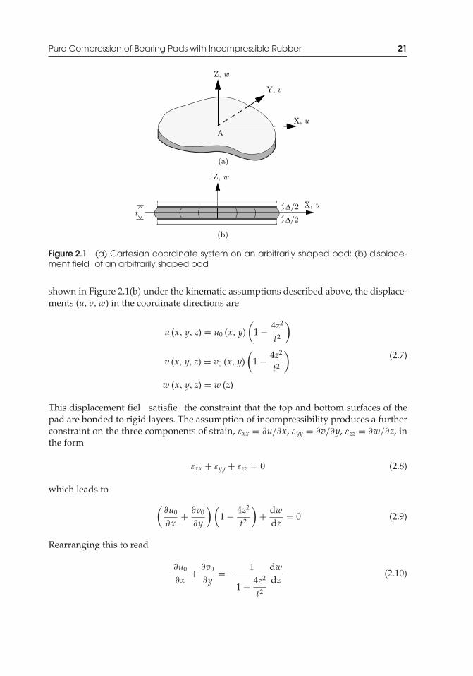
Consider an arbitrarily shaped pad of thickness t and locate, as shown in Figure 2.1(a),a rectangular Cartesian coordinate system (x, y, z) in the middle surface of the pad. As
P1: TIX/XYZ P2: ABCJWST069-02 JWST069-Kelly-Style2 July 15, 2011 14:23 Printer Name: Yet to Come
Pure Compression of Bearing Pads with Incompressible Rubber 21
Figure 2.1 (a) Cartesian coordinate system on an arbitrarily shaped pad; (b) displace-ment field of an arbitrarily shaped pad
shown in Figure 2.1(b) under the kinematic assumptions described above, the displace-ments (u, v,w) in the coordinate directions are
u (x, y, z) = u0 (x, y)(
1 − 4z2
t2
)
v (x, y, z) = v0 (x, y)(
1 − 4z2
t2
)
w (x, y, z) = w (z)
(2.7)
This displacement fiel satisfie the constraint that the top and bottom surfaces of thepad are bonded to rigid layers. The assumption of incompressibility produces a furtherconstraint on the three components of strain, εxx = ∂u/∂x, εyy = ∂v/∂y, εzz = ∂w/∂z, inthe form
εxx + εyy + εzz = 0 (2.8)
which leads to(
∂u0
∂x+ ∂v0
∂y
)(1 − 4z2
t2
)+ dw
dz= 0 (2.9)
Rearranging this to read
∂u0
∂x+ ∂v0
∂y= − 1
1 − 4z2
t2
dwdz
(2.10)
P1: TIX/XYZ P2: ABCJWST069-02 JWST069-Kelly-Style2 July 15, 2011 14:23 Printer Name: Yet to Come
22 Behavior of Multilayer Rubber Bearings under Compression
we see that we have a function of x and y on the left-hand side and a function of z onthe right, and since the equation is an identity that holds everywhere, both sides mustequal a constant k. To determine k, we solve
dwdz
= −k(
1 − 4z2
t2
)(2.11)
to get
w(z) = −k(z− 4z3
3t2
)+ c (2.12)
where c is a constant of integration. Using the boundary conditions w(t/2) = −�/2 andw(−t/2) = �/2, we fin that c = 0 and k = 3�/(2t) = 3 εc/2, where the compressionstrain εc is define by
εc = −w (t/2) − w (−t/2)t
,(εc > 0 in compression
)(2.13)
From this we obtain the distribution of the displacement w through the thickness of thepad, if this is needed, and the integrated form of the compressibility constraint as
∂u0
∂x+ ∂v0
∂y= 3 εc
2(2.14)
The stress state is assumed to be dominated by the internal pressure, p, such that thenormal stress components, σ xx, σ yy, σ zz, differ from –p only by terms of order (t2/l2)p(where l is a characteristic length in the x−y plane), i.e.,
σxx ≈ σyy ≈ σzz ≈ −p(
1 + O(t2
l2
))(2.15)
This stress assumption gives the solution its name: pressure solution. The shear stresscomponents, τ xz and τ yz, which are generated by the constraints at the top and bottomof the pad, are assumed to be of order (t/l)p; the in-plane shear stress, τ xy, is assumed tobe of order (t2/l2)p.
The complete equations of equilibrium for the stresses are
∂σxx
∂x+ ∂τxy
∂y+ ∂τxz
∂z= 0
∂τxy
∂x+ ∂σyy
∂y+ ∂τyz
∂z= 0
∂τxz
∂x+ ∂τyz
∂y+ ∂σzz
∂z= 0
(2.16)
P1: TIX/XYZ P2: ABCJWST069-02 JWST069-Kelly-Style2 July 15, 2011 14:23 Printer Name: Yet to Come
Pure Compression of Bearing Pads with Incompressible Rubber 23
and the firs two, if we identify σ xx and σ yy, with –p, reduce under these assumptions to
∂τxz
∂z= ∂p
∂x∂τyz
∂z= ∂p
∂y
(2.17)
The third of the equations of equilibrium can be differentiated with respect to z, the orderof differentiation inverted, and Equation (2.17) substituted into the resulting equation,to give
∂2 p∂x2 + ∂2 p
∂y2 = ∇2 p = ∂2σzz
∂z2 (2.18)
Assuming that the material is linearly elastic, the shear stresses, τ xz and τ yz, are relatedto the shear strains, γ xz and γ yz, by
τxz = Gγxz, τyz = Gγyz (2.19)
with G being the shear modulus of the rubber; since γxz = ∂u/∂z+ ∂w/∂x andγyz = ∂v/∂z+ ∂w/∂y,
τxz = −8Gt2 zu0, τyz = −8G
t2 zv0 (2.20)
From the equilibrium equations, therefore,
∂p∂x
= −8Gt2
u0,∂p∂y
= −8Gt2 v0 (2.21)
which, when inverted to give u0 and v0 and inserted into the incompressibility condi-tion, give
t2
8G
(∂2 p∂x2 + ∂2 p
∂y2
)= −3 εc
2(2.22)
and this, in turn, reduces to
∂2 p∂x2 + ∂2 p
∂y2 = ∇2 p = −12Gεc
t2 (2.23)
as the partial differential equation to be satisfie by p(x, y) over the area of the pad. Theboundary condition, p = 0, on the edge of the pad completes the system for p(x, y).
P1: TIX/XYZ P2: ABCJWST069-02 JWST069-Kelly-Style2 July 15, 2011 14:23 Printer Name: Yet to Come
24 Behavior of Multilayer Rubber Bearings under Compression
To use this to determine Ec, we solve for p and integrate over the area of the pad A todetermine the resultant normal load, P. Ec is then given by
Ec = PAεc
(2.24)
The significanc of the third equation of equilibrium is now clear: with the substitutionof Equation (2.23), we have an equation for the distribution of σ zz through the thicknessof the pad in the form
∂2σzz
∂z2 = 12Gεc
t2(2.25)
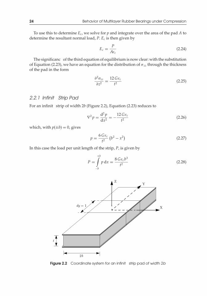
2.2.1 Infinit Strip Pad
For an infinit strip of width 2b (Figure 2.2), Equation (2.23) reduces to
∇2 p = d2 pdx2 = −12Gεc
t2 (2.26)
which, with p(±b) = 0, gives
p = 6Gεc
t2
(b2 − x2) (2.27)
In this case the load per unit length of the strip, P, is given by
P =+b∫
−bp dx = 8Gεcb3
t2(2.28)
Figure 2.2 Coordinate system for an infinit strip pad of width 2b
P1: TIX/XYZ P2: ABCJWST069-02 JWST069-Kelly-Style2 July 15, 2011 14:23 Printer Name: Yet to Come
Pure Compression of Bearing Pads with Incompressible Rubber 25
Because the shape factor, S, is b/t, and the area per unit length, A, is 2b,
Ec = PAεc
= 4GS2 (2.29)
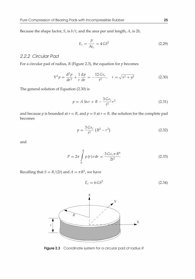
2.2.2 Circular Pad
For a circular pad of radius, R (Figure 2.3), the equation for p becomes
∇2 p = d2 pdr 2 + 1
rdpdr
= −12Gεc
t2 , r =√x2 + y2 (2.30)
The general solution of Equation (2.30) is
p = A ln r + B − 3Gεc
t2 r2 (2.31)
and because p is bounded at r = R, and p = 0 at r = R, the solution for the complete padbecomes
p = 3Gεc
t2(R2 − r 2) (2.32)
and
P = 2π
R∫0
p (r ) rdr = 3GεcπR4
2t2(2.33)
Recalling that S = R/(2t) and A = πR2, we have
Ec = 6GS2 (2.34)
Figure 2.3 Coordinate system for a circular pad of radius R
P1: TIX/XYZ P2: ABCJWST069-02 JWST069-Kelly-Style2 July 15, 2011 14:23 Printer Name: Yet to Come
26 Behavior of Multilayer Rubber Bearings under Compression
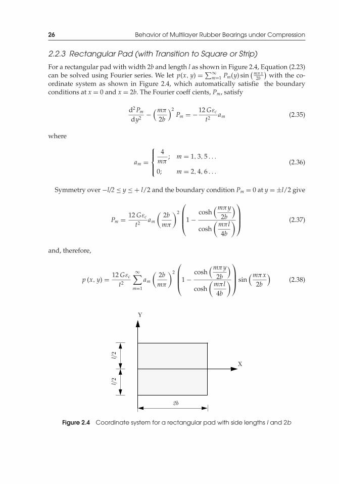
2.2.3 Rectangular Pad (with Transition to Square or Strip)
For a rectangular pad with width 2b and length l as shown in Figure 2.4, Equation (2.23)can be solved using Fourier series. We let p(x, y) =∑∞
m=1 Pm(y) sin(mπx
2b
)with the co-
ordinate system as shown in Figure 2.4, which automatically satisfie the boundaryconditions at x = 0 and x = 2b. The Fourier coeff cients, Pm, satisfy
d2Pmdy2 −
(mπ
2b
)2Pm = −12Gεc
t2 am (2.35)
where
am =
⎧⎪⎨⎪⎩
4mπ
; m = 1, 3, 5 . . .
0; m = 2, 4, 6 . . .
(2.36)
Symmetry over −l/2 ≤ y ≤ + l/2 and the boundary condition Pm = 0 at y = ±l/2 give
Pm = 12Gεc
t2 am
(2bmπ
)2
⎛⎜⎜⎝1 −
cosh(mπy
2b
)
cosh(mπl4b
)⎞⎟⎟⎠ (2.37)
and, therefore,
p (x, y) = 12Gεc
t2
∞∑m=1
am
(2bmπ
)2
⎛⎜⎜⎝1 −
cosh(mπy
2b
)
cosh(mπl4b
)⎞⎟⎟⎠ sin
(mπx2b
)(2.38)
Figure 2.4 Coordinate system for a rectangular pad with side lengths l and 2b

P1: TIX/XYZ P2: ABCJWST069-02 JWST069-Kelly-Style2 July 15, 2011 14:23 Printer Name: Yet to Come
Pure Compression of Bearing Pads with Incompressible Rubber 27
We note that the series associated with the firs term in the parenthesis is the solution of
d2 p(x)dx2 = −12Gεc
t2 (2.39)
on 0 ≤ x ≤ 2b and can be summed separately to give
p(x) = 12Gεc
t22b2(x2b
− x2
4b2
)(2.40)
giving the fina result
p(x, y) = 12Gεc
t2
⎡⎢⎢⎣2b2
(x
2b− x2
4b2
)−
∞∑m= 1,3,5...
16b2
m3π3
cosh(mπy
2b
)
cosh(mπl4b
) sin(mπx
2b
)⎤⎥⎥⎦ (2.41)
The corresponding result for Ec = P/(Aεc) is
Ec = G (2b)2
t2
⎛⎝1 −
∞∑m= 1,3,5...
192 (b/l)m5π5 tanh
(mπl4b
)⎞⎠ (2.42)
The shape factor for a rectangular pad is given by S= bl/[(l+ 2b)t], and the compressionmodulus can also be expressed in terms of the shape factor S and the aspect ratio of thebearing ρ = 2b/l as
Ec = 384π4 GS
2 (1 + ρ)2∞∑
m= odd
1m4
(1 − 2ρ
mπtanh
(mπ
2ρ
))(2.43)
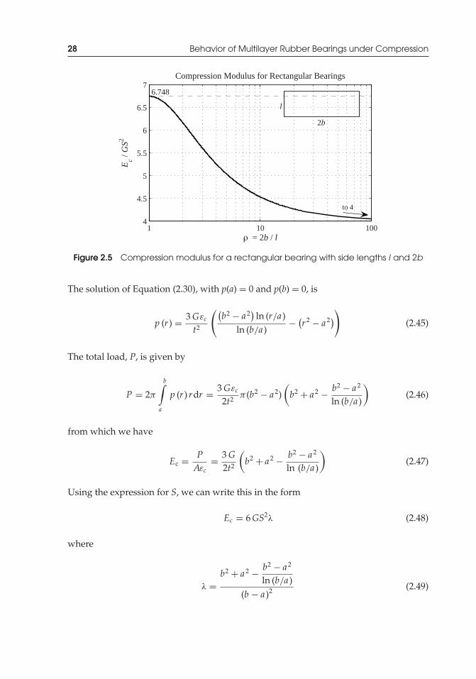
Figure 2.5 is a graph of the compression modulus as a Ec/(GS2) ratio. The graph showsthat for a square pad, Ec = 6.748GS2, while for an infinit strip, Ec = 4GS2, which is inagreement with Equation (2.29).
2.2.4 Annular Pad
Consider an annular pad with inner radius a, outer radius b, and thickness t. The shapefactor in this case is
S = π(b2 − a2
)2π (a + b) t
= b − a2t
(2.44)
P1: TIX/XYZ P2: ABCJWST069-02 JWST069-Kelly-Style2 July 15, 2011 14:23 Printer Name: Yet to Come
28 Behavior of Multilayer Rubber Bearings under Compression
1 10 1004
4.5
5
5.5
6
6.5
7
ρ = 2b / l
Ec /
GS2
6.748
Compression Modulus for Rectangular Bearings
to 4
l
2b
Figure 2.5 Compression modulus for a rectangular bearing with side lengths l and 2b
The solution of Equation (2.30), with p(a) = 0 and p(b) = 0, is
p (r ) = 3Gεc
t2
((b2 − a2
)ln (r/a )
ln (b/a )− (r2 − a2)
)(2.45)
The total load, P, is given by
P = 2π
b∫a
p (r ) rdr = 3Gεc
2t2π (b2 − a2)
(b2 + a2 − b2 − a2
ln (b/a )
)(2.46)
from which we have
Ec = PAεc
= 3G2t2
(b2 + a2 − b2 − a2
ln (b/a )
)(2.47)
Using the expression for S, we can write this in the form
Ec = 6GS2λ (2.48)
where
λ =b2 + a2 − b2 − a2
ln (b/a )(b − a )2 (2.49)
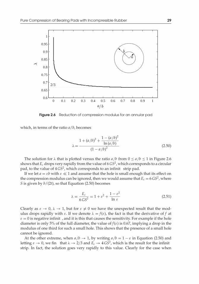
P1: TIX/XYZ P2: ABCJWST069-02 JWST069-Kelly-Style2 July 15, 2011 14:23 Printer Name: Yet to Come
Pure Compression of Bearing Pads with Incompressible Rubber 29
0 0.1 0.2 0.3 0.4 0.5 0.6 0.7 0.8 0.9 10.6
0.65
0.7
0.75
0.8
0.85
0.9
0.95
1
2/3
Figure 2.6 Reduction of compression modulus for an annular pad
which, in terms of the ratio a/b, becomes
λ =1 + (a/b)2 + 1 − (a/b)2
ln (a/b)(1 − a/b)2 (2.50)
The solution for λ that is plotted versus the ratio a/b from 0 ≤ a/b ≤ 1 in Figure 2.6shows that Ec drops very rapidly from the value of 6GS2, which corresponds to a circularpad, to the value of 4GS2, which corresponds to an infinit strip pad.
If we let a = εb with ε � 1 and assume that the hole is small enough that its effect onthe compression modulus can be ignored, then we would assume that Ec = 6GS2, whereS is given by b/(2t), so that Equation (2.50) becomes
λ = Ec6GS2 = 1 + ε2 + 1 − ε2
ln ε(2.51)
Clearly as ε → 0, λ → 1, but for ε = 0 we have the unexpected result that the mod-ulus drops rapidly with ε. If we denote λ = f (ε), the fact is that the derivative of f atε = 0 is negative infinit , and it is this that causes the sensitivity. For example if the holediameter is only 5% of the full diameter, the value of f (ε) is 0.67, implying a drop in themodulus of one third for such a small hole. This shows that the presence of a small holecannot be ignored.
At the other extreme, when a/b → 1, by writing a/b = 1 − ε in Equation (2.50) andletting ε → 0, we fin that λ → 2/3 and Ec → 4GS2, which is the result for the infinitstrip. In fact, the solution goes very rapidly to this value. Clearly for the case when
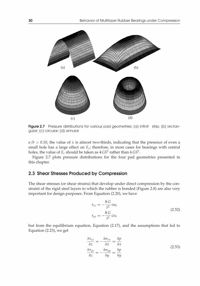
P1: TIX/XYZ P2: ABCJWST069-02 JWST069-Kelly-Style2 July 15, 2011 14:23 Printer Name: Yet to Come
30 Behavior of Multilayer Rubber Bearings under Compression
(a) (b)
(c) (d)
Figure 2.7 Pressure distributions for various pad geometries: (a) infinit strip; (b) rectan-gular; (c) circular; (d) annular
a/b > 0.10, the value of λ is almost two-thirds, indicating that the presence of even asmall hole has a large effect on Ec; therefore, in most cases for bearings with centralholes, the value of Ec should be taken as 4GS2 rather than 6GS2.
Figure 2.7 plots pressure distributions for the four pad geometries presented inthis chapter.
2.3 Shear Stresses Produced by Compression
The shear stresses (or shear strains) that develop under direct compression by the con-straint of the rigid steel layers to which the rubber is bonded (Figure 2.8) are also veryimportant for design purposes. From Equation (2.20), we have
τxz = −8Gt2 zu0
τyz = −8Gt2 zv0
(2.52)
but from the equilibrium equation, Equation (2.17), and the assumptions that led toEquation (2.23), we get
∂τxz
∂z= −∂σxx
∂x= ∂p
∂x∂τyz
∂z= −∂σyy
∂y= ∂p
∂y
(2.53)

P1: TIX/XYZ P2: ABCJWST069-02 JWST069-Kelly-Style2 July 15, 2011 14:23 Printer Name: Yet to Come
Shear Stresses Produced by Compression 31
Figure 2.8 Shear stresses produced by pure compression
Given p, these equations can be used to determine the shear stress or shear straindistribution, particularly the maximum shear stress and shear strain.
For the infinit strip of width 2b, where
p = 6Gεc
t2
(b2 − x2) (2.54)
we have
τxz = −12Gεc
t2 xz (2.55)
and the maximum value occurs at x = b, z = t/2, giving
τmax = 6Gεcbt
(2.56)
In terms of S, the maximum shear strain is given by
γmax = 6 Sεc = γc (2.57)
Thus, the compression strain causes a shear strain with a peak value 6S times greater,and since S can be quite large for a thin pad, the multiplying factor will be correspond-ingly large.
For a circular pad, we have
p = 3Gεc
t2
[R2 − (x2 + y2)] (2.58)
and
τxz = −6Gεc
t2xz, τyz = −6Gεc
t2 yz (2.59)
P1: TIX/XYZ P2: ABCJWST069-02 JWST069-Kelly-Style2 July 15, 2011 14:23 Printer Name: Yet to Come
32 Behavior of Multilayer Rubber Bearings under Compression
The maximum shear stress occurs at the top and bottom edges of the periphery of thepad and is
τmax = 3Gεc Rt
(2.60)
which is equivalent to
γc = 6 Sεc (2.61)
as before. These results can be used to establish a maximum strain criterion for therubber. For example, some bridge-bearing design codes denote the shear strain due toshear deformation of the pad by γ s, which when added to the shear strain produced bycompression, γ c, is used to defin a maximum strain unit, such as, for example,
γs + γc ≤ 0.5εbr (2.62)
where εbr is the elongation to break of the rubber.The maximum shear strain due to compression is not the only shear strain quantity
of interest to the designer. It is also useful to have an estimate of the average strain forthe following reason: because rubber is somewhat strain sensitive, G is often modifieaccording to the strain level, particularly in highly fille rubbers. In compression, theshear strain varies from positive to negative over the volume of the pad in such a waythat the simple average is zero; therefore, the appropriate average is the square root ofthe integrated squared strains. We defin γave through the integral
γ 2ave = 1
At
∫Vol
(γ 2xz + γ 2
yz
)dV (2.63)
On the other hand the total elastic stored energy, U, in the pad is given by
U = 12G
∫A
∫t
(τ 2xz + τ 2
yz
)dzdA (2.64)
so that the average shear strain, γave, can be obtained from
U = 12Gγ 2
aveAt (2.65)
But the total elastic stored energy is in turn equal to the external work P�/2, from which
U = 12Gγ 2
ave = At = 12
(Ec Aεc) (εc t) (2.66)
P1: TIX/XYZ P2: ABCJWST069-02 JWST069-Kelly-Style2 July 15, 2011 14:23 Printer Name: Yet to Come
Pure Compression of Single Pads with Compressible Rubber 33
Therefore,
γ 2ave = Ec
Gε2c (2.67)
For the strip, we have
γave = 2 Sεc (2.68)
and for the circular pad,
γave =√
6 Sεc (2.69)
Although a certain degree of trial and error is needed, computations of this kind allowthe designer to estimate the appropriate value of G, which can then be used to estimatethe vertical stiffness. First, we must assume a value of G in order to calculate εc, andfrom that calculate γave; we then modifyG and iterate as necessary. Because the modulusis not very sensitive to strain above about 20%, few iterations are needed.
2.4 Pure Compression of Single Pads with Compressible Rubber
The theory for the compression of a rubber pad given in this section is based on twoassumptions: first the displacement pattern determined in Equation (2.7); second, thenormal stress components in all three directions can be approximated by the pressure,p, in the material. Integration through the thickness of the pad of the equation ofincompressibility leads to an equation for p(x,y). To include the influenc of bulkcompressibility, we need only replace the equation of incompressibility constraint,Equation (2.8), by
εxx + εyy + εzz = − pK
(2.70)
where K is the bulk modulus. Integration through the thickness leads to
∇2 p − 12GKt2
p = −12Gεc
t2 (2.71)
that is solved, as before, with p = 0 on the edge of the pad.
2.4.1 Infinit Strip Pad
For an infinit strip, –b≤ x≤ b, of thickness t, the solution for p is of the form (Chalhouband Kelly 1991)
p = K εc
(1 − cosh (λx)
cosh (λb)
)(2.72)
P1: TIX/XYZ P2: ABCJWST069-02 JWST069-Kelly-Style2 July 15, 2011 14:23 Printer Name: Yet to Come
34 Behavior of Multilayer Rubber Bearings under Compression
where λ2 = 12G/(Kt2). Integrating p over the area of the pad gives
P =+b∫
−bp(x) dx = 2K εcb
(1 − 1
λbtanh (λb)
)(2.73)
and
Ec = K(
1 − 1λb
tanh (λb))
(2.74)
In terms of the shape factor, S, here taken as b/t, we have
λb =√
12GK
S (2.75)
and then Equation (2.74) can be expressed as
Ec = K
⎛⎜⎜⎜⎜⎝1 −
tanh
(√12GK
S
)
√12GK
S
⎞⎟⎟⎟⎟⎠ (2.76)
For small values of the parameter x, tanh x can be approximated by
tanh x = x − x3
3+ 2x5
15+ · · ·
Thus,
1 − 1x
tanh x = x2
3− 2x4
15
and from this, Ec can be approximated by
Ec = 4GS2
(1 − 24GS2
5K
)(2.77)
For example, for a fille rubber with G = 1.0 MPa (145 psi), K = 2000 MPa (289 855 psi),and a shape factor of 10, the contribution provided by the second term in Equation (2.77)is 24%.
P1: TIX/XYZ P2: ABCJWST069-02 JWST069-Kelly-Style2 July 15, 2011 14:23 Printer Name: Yet to Come
Pure Compression of Single Pads with Compressible Rubber 35
The recommended ad hoc modificatio (Lindley 1966) for the effect of bulk compress-ibility is
1Ec
= 1E∞c
+ 1K
(2.78)
where E∞c is the effective compression modulus assuming incompressibility. The ap-
proximation for small S can be inverted to give
1Ec
= 1
4GS2
(1 − 24GS2
5K
) (2.79)
which, in turn, can be approximated by
1Ec
= 1
4GS2 + 65K
(2.80)
indicating that the ad hoc modificatio is not completely correct. For very large values ofS, where (12GS2/K)1/2 ≥ 1,
Ec = K
[1 −
√K
12GS2
](2.81)
showing that K is an upper bound to Ec.The effect of the shape factor on the pressure distribution also confirm this result.
If we set λb � 1, and approximate cosh(λx) and cosh(λb) by Taylor’s series, clearly, thepreviously noted parabolic distribution of pressure occurs; however, if λb � 1, we canapproximate cosh(λb) by eλb/2 and cosh(λx) by eλx/2, from which
p = K εc
(1 − e−λ(b−x)
)(2.82)
implying a constant distribution of pressure across the width of the strip (except on theedges, where x = ±b, therefore, the pressure must go to zero).
When the pressure, p(x) of Equation (2.72), is normalized with the average pressure,P/(2b), then
p = pP/ (2b)
=1 − cosh (λx)
cosh (λb)
1 − tanh (λb)λb
(2.83)
Figure 2.9 shows the normalized pressure distribution, p, due to pure compression fordifferent shape factors (S = 10, 50, 500) for a strip with G = 1.0 MPa (145 psi) andK = 2000 MPa (289 855 psi).
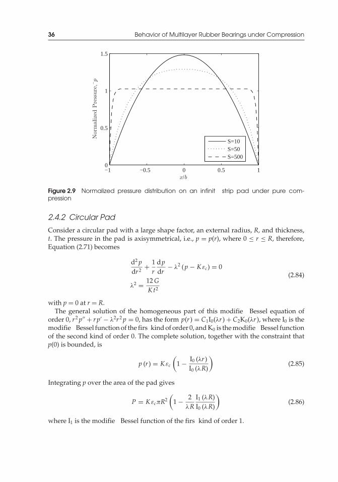
P1: TIX/XYZ P2: ABCJWST069-02 JWST069-Kelly-Style2 July 15, 2011 14:23 Printer Name: Yet to Come
36 Behavior of Multilayer Rubber Bearings under Compression
−1 −0.5 0 0.5 10
0.5
1
1.5
x/b
Nor
mal
ized
Pre
ssur
e,¯p
S=10S=50S=500
Figure 2.9 Normalized pressure distribution on an infinit strip pad under pure com-pression
2.4.2 Circular Pad
Consider a circular pad with a large shape factor, an external radius, R, and thickness,t. The pressure in the pad is axisymmetrical, i.e., p = p(r), where 0 ≤ r ≤ R, therefore,Equation (2.71) becomes
d2 pdr 2 + 1
rdpdr
− λ2 (p − K εc) = 0
λ2 = 12GKt2
(2.84)
with p = 0 at r = R.The general solution of the homogeneous part of this modifie Bessel equation of
order 0, r2 p′′ + rp′ − λ2r2 p = 0, has the form p(r ) = C1I0(λr ) + C2K0(λr ), where I0 is themodifie Bessel function of the firs kind of order 0, and K0 is the modifie Bessel functionof the second kind of order 0. The complete solution, together with the constraint thatp(0) is bounded, is
p (r ) = K εc
(1 − I0 (λr )
I0 (λR)
)(2.85)
Integrating p over the area of the pad gives
P = K εcπR2(
1 − 2λR
I1 (λR)I0 (λR)
)(2.86)
where I1 is the modifie Bessel function of the firs kind of order 1.

P1: TIX/XYZ P2: ABCJWST069-02 JWST069-Kelly-Style2 July 15, 2011 14:23 Printer Name: Yet to Come
Pure Compression of Single Pads with Compressible Rubber 37
The resulting expression for the compression modulus is
Ec = K(
1 − 2λR
I1 (λR)I0 (λR)
)(2.87)
where
λR =√
12GR2
Kt2 =√
48GK
S (2.88)
and the shape factor, S, is R/(2t). In terms of S, Equation (2.87) can be expressed as
Ec = K
⎛⎜⎜⎜⎜⎝1 − 2√
48GK
S
I1
(√48GK
S
)
I0
(√48GK
S
)
⎞⎟⎟⎟⎟⎠ (2.89)
Figure 2.10 shows graphs of Ec/(GS2) as a function of S for different K/G values.
0 5 10 15 200
1
2
3
4
5
6
7
K/G = ∞
K/G = 10000
K/G = 4000
K/G = 2500
K/G = 1000
Ec/G
S2
S
Figure 2.10 Effect of bulk compressibility on Ec for circular pads
P1: TIX/XYZ P2: ABCJWST069-02 JWST069-Kelly-Style2 July 15, 2011 14:23 Printer Name: Yet to Come
38 Behavior of Multilayer Rubber Bearings under Compression
When the argument of the modifie Bessel functions is small, the functions may beapproximated by
I1(x) = x2
(1 + x2
8+ x4
192+ · · ·
)
I0(x) =(
1 + x2
4+ x4
64+ · · ·
)
from which
2x
I1(x)I0(x)
= 1 − x2
8+ x4
48
Thus, for small values of S, the compression modulus may be estimated by
Ec = 6GS2
(1 − 8GS2
K
)(2.90)
The firs term is the standard result from the incompressibility analysis given in Equa-tion (2.34), and the second term is the correction for compressibility at moderately largeshape factors. For typical values ofG and K for fille rubbers, e.g.,G= 1.0 MPa (145 psi),K= 2000 MPa (289 855 psi), and S= 10, the second term is of order 40%. We also note that
1Ec
= 1
6GS2
(1 − 8GS2
K
) = 1
6GS2
(1 + 8GS2
K
)= 1
6GS2 + 43
1K
(2.91)
demonstrating again that the ad hoc modificatio to include compressibility is not quitecorrect. For a more exact result, K must be replaced by 3K /4 in the empirical formula.
For very large values of the argument, the modifie Bessel functions can be approxi-mated by the asymptotic expansions
I1(x) = ex√2πx
(1 − 3
8x− 15
1281x2 − · · ·
)
I0(x) = ex√2πx
(1 + 1
8x+ 9
1281x2 + · · ·
)
from which
2x
I1(x)I0(x)
= 2x
(1 − 1
2x− 1
8x2
)
P1: TIX/XYZ P2: ABCJWST069-02 JWST069-Kelly-Style2 July 15, 2011 14:23 Printer Name: Yet to Come
Pure Compression of Single Pads with Compressible Rubber 39
giving
Ec = K
⎛⎜⎜⎝1 − 1√
12GK
S
+ 148GK
S2
⎞⎟⎟⎠ (2.92)
This equation is useful when values for the modifie Bessel functions at large argumentsare not available, and it can be used with negligible error when the shape factor is greaterthan 25.
There are two points that should be mentioned about these results. The firs is that theeffect of compressibility on the compression modulus happens at such a low value ofthe shape factor. It is clear that bulk compressibility must be included for pads withshape factors a low as 10. In current practice, bearings tend to have shape factors in therange 30–40, where the compressibility will play a very large role. The other point is thatthe ad hoc approximation is not very accurate and that the designer should use the Besselfunction solution, which is not the usual practice. There is the further complication thatwe need a good estimate of the value of the bulk modulus, K, when designing thesehigh-shape-factor bearings, but this quantity is very difficul to measure, and estimatesin the literature vary widely, for example from 1000 to 3500 MPa. To provide accurateestimates of the vertical frequency or the buckling load, covered in Chapters 5 and 6, abetter estimate is needed, although it is not yet available.
2.4.3 Rectangular Pad
To compute the effective stiffness, Ec, for a rectangular pad (as shown in Figure 2.4) witha large shape factor, we f rst solve Equation (2.71) by using the same rapidly convergentsingle series solution, p(x, y) =∑∞
m=1 Pm(y) sin(mπx
2b
), used to develop the earlier result
for incompressible rubber. The Fourier coefficients Pm(y), must satisfy
d2Pmdy2 − β2
mPm = −12Gεc
t2 am (2.93)
where am = 4/(mπ ) for odd m and zero otherwise, and β2m = [mπ/(2b)]2 + 12G/(Kt2).
After solving for Pm, the pressure distribution takes the fina form
p = (x, y) = 12Gεc
t2
∞∑m=1
amβ2m
⎛⎜⎜⎝1 − cosh (βmy)
cosh(
βml2
)⎞⎟⎟⎠ sin
(mπx2b
)(2.94)
P1: TIX/XYZ P2: ABCJWST069-02 JWST069-Kelly-Style2 July 15, 2011 14:23 Printer Name: Yet to Come
40 Behavior of Multilayer Rubber Bearings under Compression
Integrating over the domain,
P =l/2∫
−l/2
2b∫0
p (x, y) dx dy = 12Gεc
t2
∞∑m=odd
ba2m
β2m
(l − 2
βmtanh
(βml2
))(2.95)
and using S = lb/[t(l + 2b)] and Ec = P/(Aεc), we obtain
Ec = 384π4 GS
2 (1 + ρ)2∞∑
m=odd
1m4ξ 2
m
(1 − 2ρ
mπξmtanh
(mπξm
2ρ
))(2.96)
where ρ = 2b/l is the aspect ratio of the pad, and
ξm =√
1 + 48GS2 (1 + ρ)2
K (mπ)2 (2.97)
Figure 2.11 shows Ec/(GS2) as a function of the shape factor, S, for different K/G values.The effect of bulk compressibility is pronounced, even for bearings with moderateshape factors. For example, for a rectangular pad with aspect ratio ρ = 3, shapefactor S = 20, shear modulus G = 1.0 MPa, and bulk modulus K = 2000 MPa,(i.e., K/G = 2000), Equation (2.43) which ignores bulk-compressibility effects givesEc/(GS2) = 5.62, while Equation (2.96) which takes bulk-compressibility effects intoaccount gives only Ec/(GS2) = 2.32.
2.4.4 Annular Pad
Consider a annular pad of thickness t, inner radius a, and outer radius b. The boundaryvalue problem for pressure p is
d2 pdr 2 + 1
rdpdr
− λ2 (p − K εc) = 0
p (a ) = 0, p (b) = 0(2.98)
where λ2 = 12G/(Kt2). The problem was studied by Chalhoub and Kelly (1987) andConstantinou et al. (1992). The solution of the homogeneous part of the modifie Besselequation, r2p′′ + rp′ − λ2r2p = 0, has the form p(r) = C1I0(λr) + C2K0(λr), where I0 isthe modifie Bessel function of the firs kind of order 0, and K0 is the modifie Besselfunction of the second kind of order 0. This, together with the boundary conditionsp(a) = 0 and p(b) = 0, gives the complete solution to Equation (2.98) as
p (r ) = K εc (1 + C1I0 (λr ) + C2K0 (λr )) (2.99)
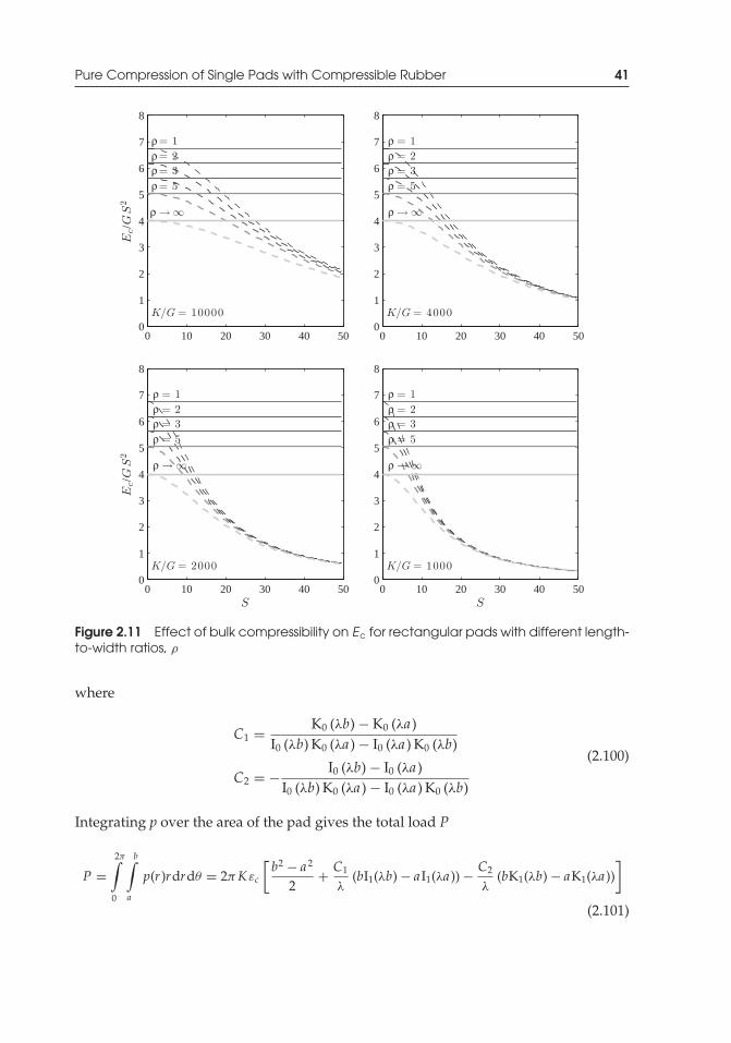
P1: TIX/XYZ P2: ABCJWST069-02 JWST069-Kelly-Style2 July 15, 2011 14:23 Printer Name: Yet to Come
Pure Compression of Single Pads with Compressible Rubber 41
0 10 20 30 40 500
1
2
3
4
5
6
7
8
ρ= 1ρ= 2ρ= 3ρ= 5
ρ →∞
K/G = 10000
Ec/G
S2
0 10 20 30 40 500
1
2
3
4
5
6
7
8
ρ = 1ρ = 2ρ = 3ρ = 5
ρ →∞
K/G = 4000
0 10 20 30 40 500
1
2
3
4
5
6
7
8
ρ = 1ρ = 2ρ = 3ρ = 5
ρ →∞
K/G = 2000
Ec/G
S2
S0 10 20 30 40 50
0
1
2
3
4
5
6
7
8
ρ = 1ρ = 2ρ = 3ρ = 5
ρ →∞
K/G = 1000
S
Figure 2.11 Effect of bulk compressibility on Ec for rectangular pads with different length-to-width ratios, ρ
where
C1 = K0 (λb) − K0 (λa )I0 (λb) K0 (λa ) − I0 (λa ) K0 (λb)
C2 = − I0 (λb) − I0 (λa )I0 (λb) K0 (λa ) − I0 (λa ) K0 (λb)
(2.100)
Integrating p over the area of the pad gives the total load P
P =2π∫
0
b∫a
p(r )rdrdθ = 2πK εc
[b2 − a 2
2+ C1
λ(bI1(λb) − a I1(λa )) − C2
λ(bK1(λb) − aK1(λa ))
]
(2.101)
P1: TIX/XYZ P2: ABCJWST069-02 JWST069-Kelly-Style2 July 15, 2011 14:23 Printer Name: Yet to Come
42 Behavior of Multilayer Rubber Bearings under Compression
and since Ec = P/(Aεc),
Ec = K[
1 + 2C1
λ2 (b2 − a2)(λbI1 (λb) − λa I1 (λa )) − 2C2
λ2 (b2 − a2)(λbK1 (λb) − λaK1 (λa ))
]
(2.102)
where I1 is the modifie Bessel function of firs kind of order 1, and K1 is the modifieBessel function of the second kind of order 1. Using S= (b – a)/(2t) and η = a/b (the ratioof the inner diameter to the outer diameter), we can express the compression modulus as
Ec = K[1 + C ′
1 (I1 (ϑ) − ηI1 (ηϑ)) + C ′2 (K1 (ϑ) − ηK1 (ηϑ))
](2.103)
where
ϑ =√
48GK
S1 − η
(2.104)
and
C ′1 = 1√
12GK
(1 + η) S
K0 (ϑ) − K0 (ηϑ)I0 (v) K0 (ηϑ) − I0 (ηϑ) K0(ϑ)
C ′2 = 1√
12GK
(1 + η) S
I0 (ϑ) − I0 (ηϑ)I0 (υ) K0 (ηϑ) −I0 (ηϑ) K0(ϑ)
(2.105)
Figure 2.12 shows graphs of the normalized compression modulus of an annular pad asa function of the shape factor, S, for different η and K/G values. The f gure shows thatfor realistic values of K/G (e.g., K/G = 2000), neglecting bulk-compressibility effectsmay grossly overestimate the compression modulus even for moderate shape factors.
We now seek to investigate the effect of a small hole on a circular pad. We firsnormalize Ec with respect to 6GS2, the value for a complete pad based on the radius R(here = b), when incompressibility is assumed and note that (λR)2 = (48GS2)/K, so that
K
6GS2 = 8
(λR)2 (2.106)
We now consider small η (i.e., <0.1) and denote it as ε. Using y= Ec/(6GS2) and x= λR,Equation (2.102) can be approximated by
y = 8x2
(1 − 2
x(K0(x) − K0 (εx)) (I1(x) − εI1(εx)) + (K1(x) − εK1 (εx)) (I0(x) − I0 (εx))
I0 (εx) K0(x) − I0(x)K0 (εx)
)
(2.107)
We now consider the particular case with G = 1.0 MPa, K = 2000 MPa and S = 20, forwhich x = 3.098. The value of the normalized modulus y when ε= 0 is 0.3936, and the
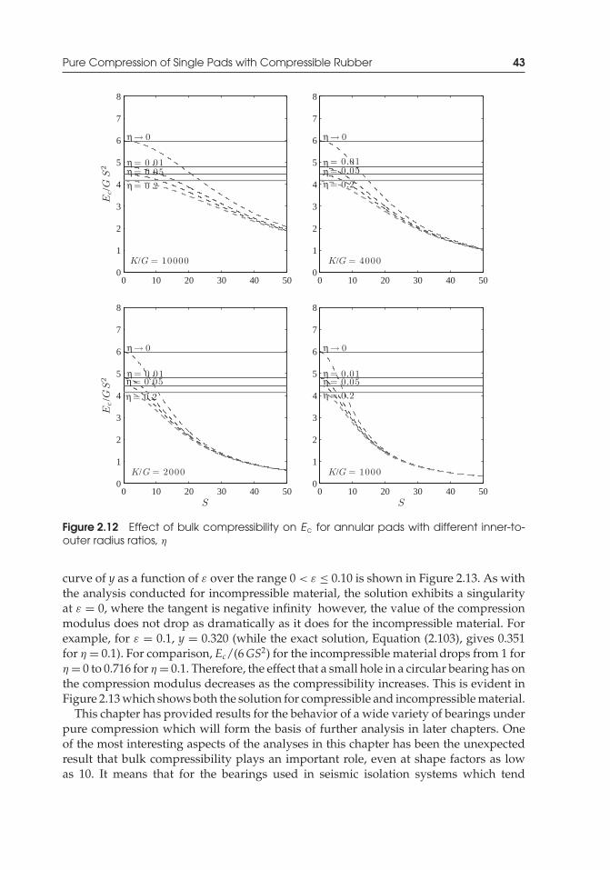
P1: TIX/XYZ P2: ABCJWST069-02 JWST069-Kelly-Style2 July 15, 2011 14:23 Printer Name: Yet to Come
Pure Compression of Single Pads with Compressible Rubber 43
0 10 20 30 40 500
1
2
3
4
5
6
7
8
η→ 0
η = 0.01η = 0.05η = 0.2
K/G = 10000
Ec/G
S2
0 10 20 30 40 500
1
2
3
4
5
6
7
8
η→ 0
η = 0 .01η = 0 .05η = 0 .2
K/G = 4000
0 10 20 30 40 500
1
2
3
4
5
6
7
8
η→ 0
η = 0.01η = 0.05
η = 0.2
K/G = 2000
Ec/G
S2
S0 10 20 30 40 50
0
1
2
3
4
5
6
7
8
η→ 0
η = 0 .01η = 0 .05η = 0 .2
K/G = 1000
S
Figure 2.12 Effect of bulk compressibility on Ec for annular pads with different inner-to-outer radius ratios, η
curve of y as a function of ε over the range 0 < ε ≤ 0.10 is shown in Figure 2.13. As withthe analysis conducted for incompressible material, the solution exhibits a singularityat ε = 0, where the tangent is negative infinity however, the value of the compressionmodulus does not drop as dramatically as it does for the incompressible material. Forexample, for ε = 0.1, y = 0.320 (while the exact solution, Equation (2.103), gives 0.351for η = 0.1). For comparison, Ec/(6GS2) for the incompressible material drops from 1 forη = 0 to 0.716 for η = 0.1. Therefore, the effect that a small hole in a circular bearing has onthe compression modulus decreases as the compressibility increases. This is evident inFigure 2.13 which shows both the solution for compressible and incompressible material.
This chapter has provided results for the behavior of a wide variety of bearings underpure compression which will form the basis of further analysis in later chapters. Oneof the most interesting aspects of the analyses in this chapter has been the unexpectedresult that bulk compressibility plays an important role, even at shape factors as lowas 10. It means that for the bearings used in seismic isolation systems which tend
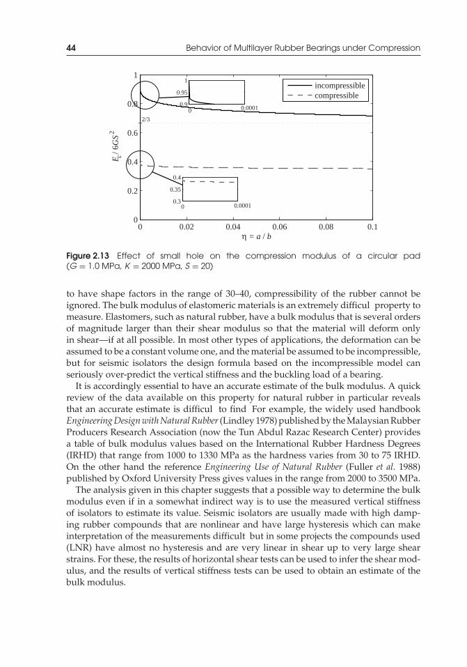
P1: TIX/XYZ P2: ABCJWST069-02 JWST069-Kelly-Style2 July 15, 2011 14:23 Printer Name: Yet to Come
44 Behavior of Multilayer Rubber Bearings under Compression
0 0.02 0.04 0.06 0.08 0.10
0.2
0.4
0.6
0.8
1
η = a / b
E c / 6
GS
2
incompressiblecompressible
00.3
0.35
0.4
0 0.00010.9
0.95
1
0.0001
2/3
Figure 2.13 Effect of small hole on the compression modulus of a circular pad(G = 1.0 MPa, K = 2000 MPa, S = 20)
to have shape factors in the range of 30–40, compressibility of the rubber cannot beignored. The bulk modulus of elastomeric materials is an extremely difficul property tomeasure. Elastomers, such as natural rubber, have a bulk modulus that is several ordersof magnitude larger than their shear modulus so that the material will deform onlyin shear—if at all possible. In most other types of applications, the deformation can beassumed to be a constant volume one, and the material be assumed to be incompressible,but for seismic isolators the design formula based on the incompressible model canseriously over-predict the vertical stiffness and the buckling load of a bearing.
It is accordingly essential to have an accurate estimate of the bulk modulus. A quickreview of the data available on this property for natural rubber in particular revealsthat an accurate estimate is difficul to find For example, the widely used handbookEngineeringDesignwithNaturalRubber (Lindley 1978) published by the Malaysian RubberProducers Research Association (now the Tun Abdul Razac Research Center) providesa table of bulk modulus values based on the International Rubber Hardness Degrees(IRHD) that range from 1000 to 1330 MPa as the hardness varies from 30 to 75 IRHD.On the other hand the reference Engineering Use of Natural Rubber (Fuller et al. 1988)published by Oxford University Press gives values in the range from 2000 to 3500 MPa.
The analysis given in this chapter suggests that a possible way to determine the bulkmodulus even if in a somewhat indirect way is to use the measured vertical stiffnessof isolators to estimate its value. Seismic isolators are usually made with high damp-ing rubber compounds that are nonlinear and have large hysteresis which can makeinterpretation of the measurements difficult but in some projects the compounds used(LNR) have almost no hysteresis and are very linear in shear up to very large shearstrains. For these, the results of horizontal shear tests can be used to infer the shear mod-ulus, and the results of vertical stiffness tests can be used to obtain an estimate of thebulk modulus.
P1: TIX/XYZ P2: ABCJWST069-03 JWST069-Kelly-Style2 July 15, 2011 16:32 Printer Name: Yet to Come
3Behavior of MultilayerRubber Bearingsunder Bending
3.1 Bending Stiffness of Single Pad with Incompressible Rubber
An important bearing property that must be analyzed for design is the buckling behaviorof the isolator. For this analysis, the response of the compressed bearing to bendingmoment is necessary. Referred to as the bending stiffness, this can be ascertained by anextension of the same analysis that is done to determine the vertical stiffness. The bendingstiffness plays an important role in the estimate of the buckling load in a bearing andalso is needed to determine the influenc of the vertical load on the horizontal (shear)stiffness of a bearing. In addition, when the isolator is subject to shear deformation, abending moment is generated by the unbalanced shear forces at the top and bottom of thebearing. These bending moments cause shear strains in the rubber that are important fordesign, and they also affect the stresses in the steel shims. In contrast to the case of purecompression, these stresses can be compressive and could produce buckling of the shims.
The bending stiffness of a single pad is computed using an approach similar to that forcompression stiffness; however, the displaced configuratio is obtained in two stages.First visualize the deformation that would occur if the bending conformed to elementarybeam theory (shown dotted in Figure 3.1). Because this cannot satisfy the incompress-ibility constraint, a further pure shear deformation is superimposed. The displacementfiel is given by
u(x, y, z) = u0(x, y)(
1 − 4z2
t2
)− αz2
2t
v(x, y, z) = v0(x, y)(
1 − 4z2
t2
)
w(x, y, z) = αzxt
(3.1)
Mechanics of Rubber Bearings for Seismic and Vibration Isolation, First Edition. James M. Kelly and Dimitrios A. Konstantinidis.C© 2011 John Wiley & Sons, Ltd. Published 2011 by John Wiley & Sons, Ltd.
45
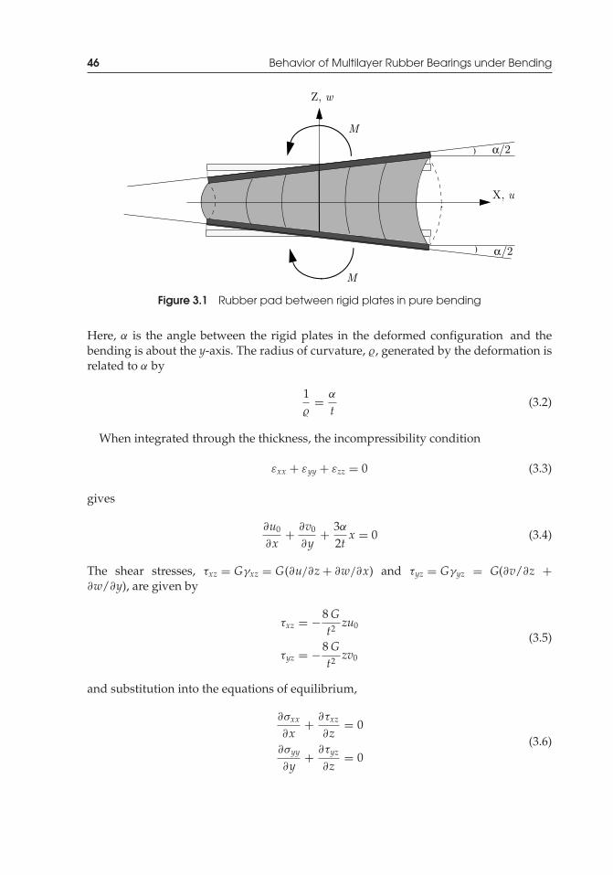
P1: TIX/XYZ P2: ABCJWST069-03 JWST069-Kelly-Style2 July 15, 2011 16:32 Printer Name: Yet to Come
46 Behavior of Multilayer Rubber Bearings under Bending
α
α
Figure 3.1 Rubber pad between rigid plates in pure bending
Here, α is the angle between the rigid plates in the deformed configuration and thebending is about the y-axis. The radius of curvature, �, generated by the deformation isrelated to α by
1�
= α
t(3.2)
When integrated through the thickness, the incompressibility condition
εxx + εyy + εzz = 0 (3.3)
gives
∂u0
∂x+ ∂v0
∂y+ 3α
2tx = 0 (3.4)
The shear stresses, τxz = Gγxz = G(∂u/∂z+ ∂w/∂x) and τyz = Gγyz = G(∂v/∂z +∂w/∂y), are given by
τxz = −8Gt2 zu0
τyz = −8Gt2 zv0
(3.5)
and substitution into the equations of equilibrium,
∂σxx
∂x+ ∂τxz
∂z= 0
∂σyy
∂y+ ∂τyz
∂z= 0
(3.6)
P1: TIX/XYZ P2: ABCJWST069-03 JWST069-Kelly-Style2 July 15, 2011 16:32 Printer Name: Yet to Come
Bending Stiffness of Single Pad with Incompressible Rubber 47
gives
u0 = − t2
8G∂p∂x
, v0 = − t2
8G∂p∂y
(3.7)
which, with the incompressibility condition, leads to
∂2 p∂x2 + ∂2 p
∂y2 = ∇2 p = 12Gα
t3 x (3.8)
with p = 0 on the edges.The solution technique is to solve Equation (3.8) for p and to compute the bending
moment M from
M = −∫A
p(x, y)xdA (3.9)
Using the analogy with beam theory, where
M = EI1�
(3.10)
we compute the bending stiffness
(EI)eff = Mα/t
(3.11)
3.1.1 Infinit Strip Pad
For the example of the infinit strip of width 2b, shown in Figure 2.2, we have
d2 pdx2 = 12Gα
t3 x (3.12)
or
p = −2Gα
t3 (b2 − x2)x (3.13)
The resultant moment M is given by
M = −+b∫
−bpxdx = 8Gαb5
15t3 (3.14)
P1: TIX/XYZ P2: ABCJWST069-03 JWST069-Kelly-Style2 July 15, 2011 16:32 Printer Name: Yet to Come
48 Behavior of Multilayer Rubber Bearings under Bending
If we compare this with the usual bending equation for a beam, namely, M = EI(1/�),where I = 2b3/3 is the moment of inertia of a beam cross-section with the shape of thepad, we can obtain an effective bending stiffness (EI)eff ,
(EI)eff = M� = Mα/t
= 8Gb5
15t2 = 45GS2
(23b3
)= 4
5GIS2 (3.15)
As seen in Chapter 2, Ec = 4GS2, then (EI)eff = EcI/5. Thus, the effective I for the stripis I/5. This reduction is caused by the pressure distribution that varies cubically acrossthe width of the strip, whereas in a beam the bending stress distribution varies linearlythrough the thickness.
3.1.2 Circular Pad
For a circular pad of radius R (see Figure 2.3), the equation to be solved, using polarcoordinates r and θ , is
∂2 p∂r2 + 1
r∂p∂r
+ 1r2
∂2 p∂θ 2 = 12Gα
t3 r cos θ (3.16)
The solution is
p(r, θ ) =(Ar + B
1r
+ Cr3)
cos θ (3.17)
where
C = 3Gα
2t3
For the complete circle, 0 ≤ r≤ R, B has to be zero for p to be bounded at r= 0, and usingp = 0 at r = R gives
p = 3Gα
2t3(r2 − R2)r cos θ (3.18)
and
M = −2π∫
0
R∫0
pr2 cos(θ )drdθ = Gα
8t3 πR6 (3.19)
The effective moment of inertia in this case, taking E = Ec = 6GS2 and I = πR4/4, isone-third of the conventional moment of inertia,
(EI)eff = Mα/t
= G8t2 πR6 = 2GS2
(πR4
4
)= 2GIS2 (3.20)
Also, since for a circular pad, Ec = 6GS2, (EI)eff = EcI/3.
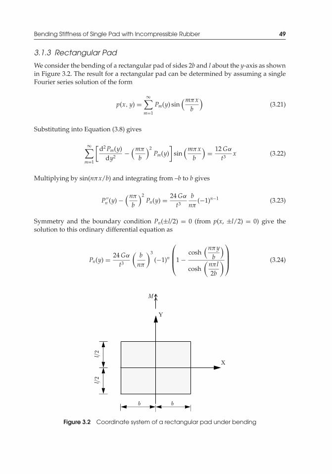
P1: TIX/XYZ P2: ABCJWST069-03 JWST069-Kelly-Style2 July 15, 2011 16:32 Printer Name: Yet to Come
Bending Stiffness of Single Pad with Incompressible Rubber 49
3.1.3 Rectangular Pad
We consider the bending of a rectangular pad of sides 2b and l about the y-axis as shownin Figure 3.2. The result for a rectangular pad can be determined by assuming a singleFourier series solution of the form
p(x, y) =∞∑m=1
Pm(y) sin(mπx
b
)(3.21)
Substituting into Equation (3.8) gives
∞∑m=1
[d2Pm(y)
dy2 −(mπ
b
)2Pm(y)
]sin
(mπxb
)= 12Gα
t3x (3.22)
Multiplying by sin(nπx/b) and integrating from –b to b gives
P ′′n (y) −
(nπb
)2Pn(y) = 24Gα
t3
bnπ
(−1)n−1 (3.23)
Symmetry and the boundary condition Pn(±l/2) = 0 (from p(x, ±l/2) = 0) give thesolution to this ordinary differential equation as
Pn(y) = 24Gα
t3
(bnπ
)3
(−1)n
⎛⎜⎜⎝1 −
cosh(nπy
b
)
cosh(nπl2b
)⎞⎟⎟⎠ (3.24)
Figure 3.2 Coordinate system of a rectangular pad under bending
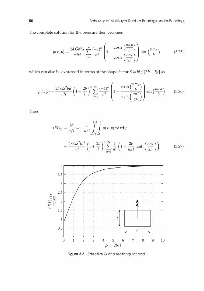
P1: TIX/XYZ P2: ABCJWST069-03 JWST069-Kelly-Style2 July 15, 2011 16:32 Printer Name: Yet to Come
50 Behavior of Multilayer Rubber Bearings under Bending
The complete solution for the pressure then becomes
p(x, y) = 24Gb3α
π3t3
∞∑n=1
(−1)n
n3
⎛⎜⎜⎝1 −
cosh(nπy
b
)
cosh(nπl2b
)⎞⎟⎟⎠ sin
(nπxb
)(3.25)
which can also be expressed in terms of the shape factor S = bl/[(2 b + l)t] as
p(x, y) = 24GS2bαπ3t
(1 + 2b
l
)2 ∞∑n=1
(−1)n
n3
⎛⎜⎜⎝1 −
cosh(nπy
b
)
cosh(nπl2b
)⎞⎟⎟⎠ sin
(nπxb
)(3.26)
Then
(EI)eff = Mα/t
= − 1α/t
l/2∫−l/2
b∫−b
p(x, y) xdxdy
= 48GS2lb3
π4
(1 + 2b
l
)2 ∞∑n=1
1n4
(1 − 2b
nπltanh
(nπl2b
))(3.27)
0 1 2 3 4 5 6 7 8 9 100
0.5
1
1.5
2
2.5
3
3.5
4
ρ = 2b/l
(EI)eff
GIS
2
2b
l
Figure 3.3 Effective EI of a rectangular pad
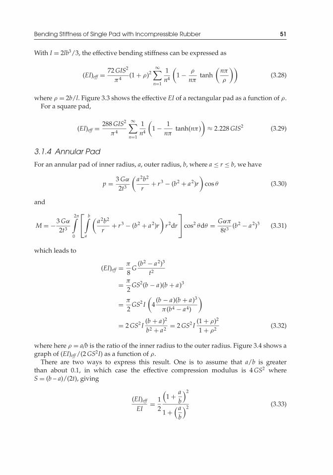
P1: TIX/XYZ P2: ABCJWST069-03 JWST069-Kelly-Style2 July 15, 2011 16:32 Printer Name: Yet to Come
Bending Stiffness of Single Pad with Incompressible Rubber 51
With I = 2lb3/3, the effective bending stiffness can be expressed as
(EI)eff = 72GIS2
π4 (1 + ρ)2∞∑n=1
1n4
(1 − ρ
nπtanh
(nπρ
))(3.28)
where ρ = 2b/l. Figure 3.3 shows the effective EI of a rectangular pad as a function of ρ.For a square pad,
(EI)eff = 288GIS2
π4
∞∑n=1
1n4
(1 − 1
nπtanh(nπ )
)≈ 2.228GIS2 (3.29)
3.1.4 Annular Pad
For an annular pad of inner radius, a, outer radius, b, where a ≤ r ≤ b, we have
p = 3Gα
2t3
(a 2b2
r+ r3 − (b2 + a2)r
)cos θ (3.30)
and
M = −3Gα
2t3
2π∫0
⎡⎣
b∫a
(a 2b2
r+ r3 − (b2 + a2)r
)r2dr
⎤⎦ cos2 θdθ = Gαπ
8t3(b2 − a 2)3 (3.31)
which leads to
(EI)eff = π
8G
(b2 − a2)3
t2
= π
2GS2(b − a )(b + a )3
= π
2GS2 I
(4
(b − a )(b + a )3
π (b4 − a4)
)
= 2GS2 I(b + a )2
b2 + a2 = 2GS2 I(1 + ρ)2
1 + ρ2 (3.32)
where here ρ = a/b is the ratio of the inner radius to the outer radius. Figure 3.4 shows agraph of (EI)eff/(2GS2I) as a function of ρ.
There are two ways to express this result. One is to assume that a/b is greaterthan about 0.1, in which case the effective compression modulus is 4GS2 whereS = (b – a)/(2t), giving
(EI)effEI
= 12
(1 + a
b
)2
1 +(ab
)2 (3.33)

P1: TIX/XYZ P2: ABCJWST069-03 JWST069-Kelly-Style2 July 15, 2011 16:32 Printer Name: Yet to Come
52 Behavior of Multilayer Rubber Bearings under Bending
0 0.1 0.2 0.3 0.4 0.5 0.6 0.7 0.8 0.9 12
2.2
2.4
2.6
2.8
3
3.2
3.4
3.6
3.8
4
ρ = a/b
(EI)eff
GIS
2
Figure 3.4 Effective EI of an annular pad with inner radius a and outer radius b
On the other hand, if a → 0, then (EI)eff → 6GS2(I/3). In addition, if we write a = bεand let ε → 0, we get (EI)eff → 4GS2(1 + 2ε) (I/2), showing that in contrast to case ofthe compression modulus, the presence of a small hole has a negligible effect on thebending stiffness. The reason, of course, is that the pressure at the edge of the hole, if itis small, is very close to zero anyway, and the boundary condition of zero pressure isalready met.
3.2 Bending Stiffness of Single Pads with Compressible Rubber
If we take into account the bulk compressibility when estimating the bending stiffness,the equation to be solved is
∇2 p − λ2 p = λ2Kα
tx (3.34)
where λ2 = 12G/(Kt2) and p = 0 at the edge of the pad.
3.2.1 Infinit Strip Pad
For an infinit strip of width 2b, Equation (3.34) becomes
d2 pdx2 − λ2 p = λ2Kα
tx (3.35)
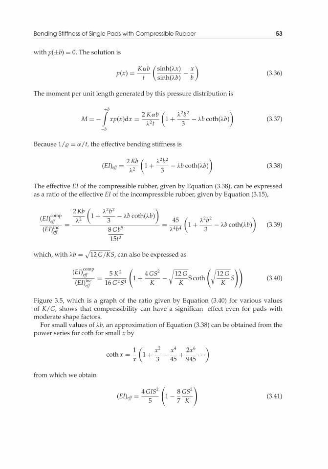
P1: TIX/XYZ P2: ABCJWST069-03 JWST069-Kelly-Style2 July 15, 2011 16:32 Printer Name: Yet to Come
Bending Stiffness of Single Pads with Compressible Rubber 53
with p(±b) = 0. The solution is
p(x) = Kαbt
(sinh(λx)sinh(λb)
− xb
)(3.36)
The moment per unit length generated by this pressure distribution is
M = −+b∫
−bxp(x)dx = 2 Kαb
λ2t
(1 + λ2b2
3− λb coth(λb)
)(3.37)
Because 1/� = α/t, the effective bending stiffness is
(EI)eff = 2Kbλ2
(1 + λ2b2
3− λb coth(λb)
)(3.38)
The effective EI of the compressible rubber, given by Equation (3.38), can be expressedas a ratio of the effective EI of the incompressible rubber, given by Equation (3.15),
(EI)compeff
(EI)inceff
=2Kbλ2
(1 + λ2b2
3− λb coth(λb)
)
8Gb5
15t2
= 45λ4b4
(1 + λ2b2
3− λb coth(λb)
)(3.39)
which, with λb = √12G/KS, can also be expressed as
(EI)compeff
(EI)inceff
= 5 K 2
16G2S4
(1 + 4GS2
K−
√12GK
S coth
(√12GK
S
))(3.40)
Figure 3.5, which is a graph of the ratio given by Equation (3.40) for various valuesof K/G, shows that compressibility can have a significan effect even for pads withmoderate shape factors.
For small values of λb, an approximation of Equation (3.38) can be obtained from thepower series for coth for small x by
coth x = 1x
(1 + x2
3− x4
45+ 2x6
945· · ·
)
from which we obtain
(EI)eff = 4GIS2
5
(1 − 8
7GS2
K
)(3.41)
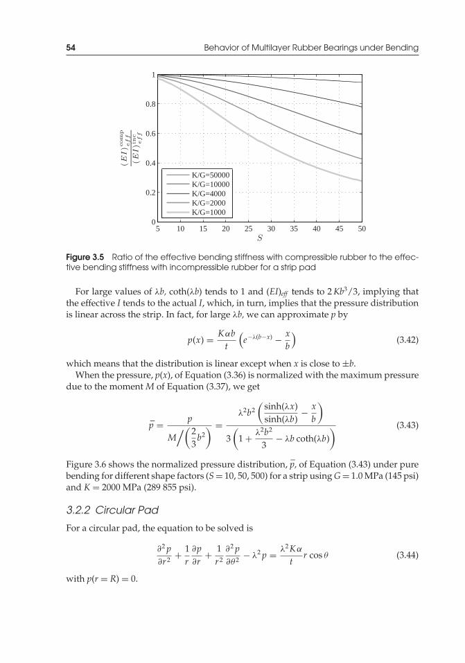
P1: TIX/XYZ P2: ABCJWST069-03 JWST069-Kelly-Style2 July 15, 2011 16:32 Printer Name: Yet to Come
54 Behavior of Multilayer Rubber Bearings under Bending
5 10 15 20 25 30 35 40 45 500
0.2
0.4
0.6
0.8
1
S
(EI)co
mp
eff
(EI)in
ceff
K/G=50000K/G=10000K/G=4000K/G=2000K/G=1000
Figure 3.5 Ratio of the effective bending stiffness with compressible rubber to the effec-tive bending stiffness with incompressible rubber for a strip pad
For large values of λb, coth(λb) tends to 1 and (EI)eff tends to 2Kb3/3, implying thatthe effective I tends to the actual I, which, in turn, implies that the pressure distributionis linear across the strip. In fact, for large λb, we can approximate p by
p(x) = Kαbt
(e−λ(b−x) − x
b
)(3.42)
which means that the distribution is linear except when x is close to ±b.When the pressure, p(x), of Equation (3.36) is normalized with the maximum pressure
due to the moment M of Equation (3.37), we get
p = p
M/(
23b2
) =λ2b2
(sinh(λx)sinh(λb)
− xb
)
3(
1 + λ2b2
3− λb coth(λb)
) (3.43)
Figure 3.6 shows the normalized pressure distribution, p, of Equation (3.43) under purebending for different shape factors (S= 10, 50, 500) for a strip usingG= 1.0 MPa (145 psi)and K = 2000 MPa (289 855 psi).
3.2.2 Circular Pad
For a circular pad, the equation to be solved is
∂2 p∂r 2 + 1
r∂p∂r
+ 1r2
∂2 p∂θ2 − λ2 p = λ2Kα
tr cos θ (3.44)
with p(r = R) = 0.
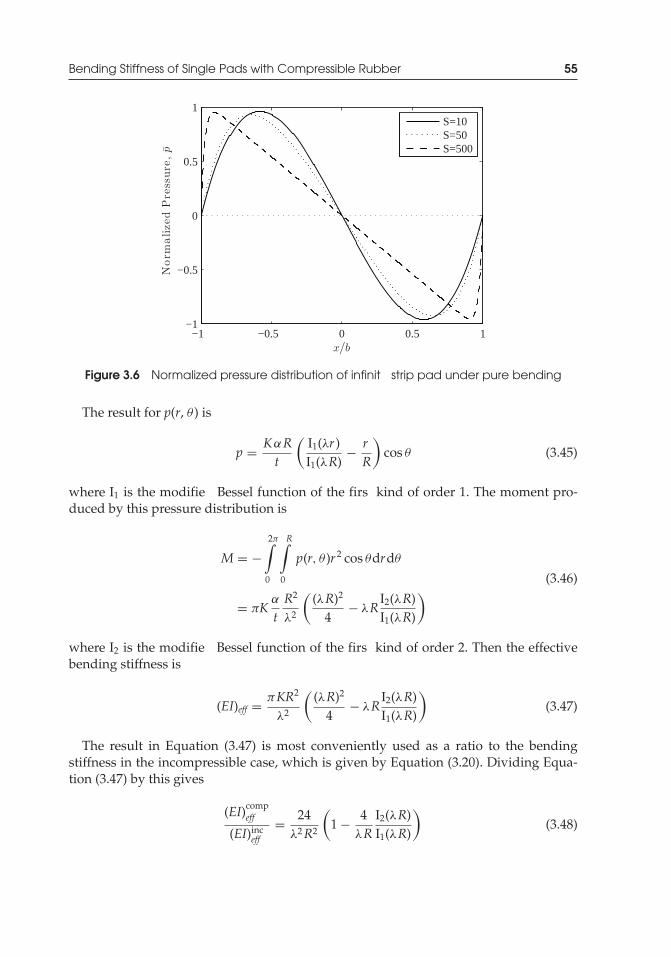
P1: TIX/XYZ P2: ABCJWST069-03 JWST069-Kelly-Style2 July 15, 2011 16:32 Printer Name: Yet to Come
Bending Stiffness of Single Pads with Compressible Rubber 55
−1 −0.5 0 0.5 1−1
−0.5
0
0.5
1
x/b
Nor
mal
ized
Pre
ssur
e,p
S=10S=50S=500
Figure 3.6 Normalized pressure distribution of infinit strip pad under pure bending
The result for p(r, θ ) is
p = KαRt
(I1(λr )I1(λR)
− rR
)cos θ (3.45)
where I1 is the modifie Bessel function of the firs kind of order 1. The moment pro-duced by this pressure distribution is
M = −2π∫
0
R∫0
p(r, θ )r2 cos θdrdθ
= πKα
tR2
λ2
((λR)2
4− λR
I2(λR)I1(λR)
) (3.46)
where I2 is the modifie Bessel function of the firs kind of order 2. Then the effectivebending stiffness is
(EI)eff = πKR2
λ2
((λR)2
4− λR
I2(λR)I1(λR)
)(3.47)
The result in Equation (3.47) is most conveniently used as a ratio to the bendingstiffness in the incompressible case, which is given by Equation (3.20). Dividing Equa-tion (3.47) by this gives
(EI)compeff
(EI)inceff
= 24λ2R2
(1 − 4
λRI2(λR)I1(λR)
)(3.48)
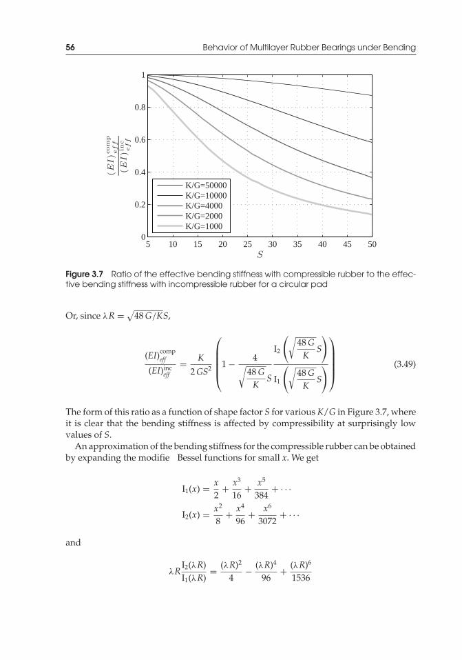
P1: TIX/XYZ P2: ABCJWST069-03 JWST069-Kelly-Style2 July 15, 2011 16:32 Printer Name: Yet to Come
56 Behavior of Multilayer Rubber Bearings under Bending
5 10 15 20 25 30 35 40 45 500
0.2
0.4
0.6
0.8
1
S
(EI)co
mp
eff
(EI)in
ceff
K/G=50000K/G=10000K/G=4000K/G=2000K/G=1000
Figure 3.7 Ratio of the effective bending stiffness with compressible rubber to the effec-tive bending stiffness with incompressible rubber for a circular pad
Or, since λR = √48G/KS,
(EI)compeff
(EI)inceff
= K
2GS2
⎛⎜⎜⎜⎜⎝1 − 4√
48GK
S
I2
(√48GK
S
)
I1
(√48GK
S
)
⎞⎟⎟⎟⎟⎠ (3.49)
The form of this ratio as a function of shape factor S for various K/G in Figure 3.7, whereit is clear that the bending stiffness is affected by compressibility at surprisingly lowvalues of S.
An approximation of the bending stiffness for the compressible rubber can be obtainedby expanding the modifie Bessel functions for small x. We get
I1(x) = x2
+ x3
16+ x5
384+ · · ·
I2(x) = x2
8+ x4
96+ x6
3072+ · · ·
and
λRI2(λR)I1(λR)
= (λR)2
4− (λR)4
96+ (λR)6
1536
P1: TIX/XYZ P2: ABCJWST069-03 JWST069-Kelly-Style2 July 15, 2011 16:32 Printer Name: Yet to Come
Bending Stiffness of Single Pads with Compressible Rubber 57
leading to
(EI)eff = 2GIS2
(1 − 3GS2
K
)(3.50)
For very large values of x, both I1 and I2 tend to ex/√
2πx, and the asymptotic value of(EI)eff is KI, which is what would be expected if the pressure distribution was linear andthe compression modulus was K. In fact, for large values of S, the pressure distributiondoes tend to be linear, as shown by Equation (3.45), which when λ → ∞, tends to
p = −Kα
tr cos θ (3.51)
3.2.3 Rectangular Pad
The result for a rectangular pad (Figure 3.2) can be determined by assuming a singleFourier series solution of the form
p(x, y) =∞∑m=1
Pm(y) sin(mπx
b
)(3.52)
Substituting this into Equation (3.34) gives
∞∑m=1
{d2Pm(y)
dy2 −[(mπ
b
)2+ λ2
]Pm(y)
}sin
(mπxb
)= λ2Kα
tx (3.53)
Multiplying by sin(nπx/b) and integrating from –b to b gives
d2Pn(y)dy2 − β2
n Pn(y) = 2λ2Kαbnπ t
(−1)n−1 (3.54)
where β2n = (nπ/b)2 + λ2. Symmetry and the boundary condition Pn(±l/2) = 0 (from
p(x, ±l/2) = 0) give the solution to this ordinary differential equation as
Pn(y) = 2λ2Kαbnπ tβ2
n(−1)n
(1 − cosh(βny)
cosh(βnl/2)
)(3.55)
The complete solution for the pressure becomes
p(x, y) = 2λ2Kαbt
∞∑n=1
(−1)n
nπβ2n
[1 − cosh(βny)
cosh(βnl/2)
]sin
(nπxb
)(3.56)
P1: TIX/XYZ P2: ABCJWST069-03 JWST069-Kelly-Style2 July 15, 2011 16:32 Printer Name: Yet to Come
58 Behavior of Multilayer Rubber Bearings under Bending
Then
(EI)eff = Mα/t
= − 1α/t
l/2∫−l/2
b∫−b
p(x, y)xdxdy
= 4λ2Klb3
π2
∞∑n=1
1n2β2
n
(1 − 2
βnltanh
(βnl2
))
= 48GS2lbπ2
(1 + 2b
l
)2 ∞∑n=1
1n2β2
n
(1 − 2
βnltanh
(βnl2
))(3.57)
To examine the effect of compressibility on the bending stiffness, we can expressEquation (3.57) as a ratio to the effective EI for incompressible material, Equa-tion (3.27), obtaining
(EI)compeff
(EI)inceff
=
∞∑n=1
1
n4
(1 + 12GS2
n2π2K(1 + ρ)2
)
⎡⎢⎢⎢⎢⎢⎢⎣
1 − ρ
nπ
tanh
⎛⎝nπ
ρ
√1 + 12GS2
n2π2K(1 + ρ)2
⎞⎠
√1 + 12GS2
n2π2K(1 + ρ)2
⎤⎥⎥⎥⎥⎥⎥⎦
∞∑n=1
1n4
(1 − ρ
nπtanh
(nπρ
))
(3.58)
where ρ = 2b/l. Figure 3.8 shows graphs of (EI)compeff /(EI)inc
eff versus S for different K/Gand ρ values.
3.2.4 Annular Pad
For an annular pad of inner radius a, outer radius b, where a ≤ r ≤ b, Equa-tion (3.34) becomes
∂2 p∂r 2 + 1
r∂p∂r
+ 1r2
∂2 p∂θ2 − λ2 p = λ2 Kα
tr cos θ (3.59)
with boundary conditions p(a, θ ) = p(b, θ ) = 0. Assuming a solution of the form
p(r, θ ) = f (r )cosθ (3.60)
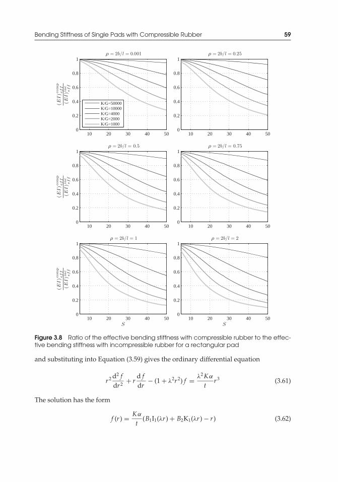
P1: TIX/XYZ P2: ABCJWST069-03 JWST069-Kelly-Style2 July 15, 2011 16:32 Printer Name: Yet to Come
Bending Stiffness of Single Pads with Compressible Rubber 59
10 20 30 40 500
0.2
0.4
0.6
0.8
1(EI)co
mp
eff
(EI)in
ceff
ρ = 2b/l = 0.001
K/G=50000K/G=10000K/G=4000K/G=2000K/G=1000
10 20 30 40 500
0.2
0.4
0.6
0.8
1ρ = 2b/l = 0.25
10 20 30 40 500
0.2
0.4
0.6
0.8
1
(EI)co
mp
eff
(EI)in
ceff
ρ = 2b/l = 0.5
10 20 30 40 500
0.2
0.4
0.6
0.8
1ρ = 2b/l = 0.75
10 20 30 40 500
0.2
0.4
0.6
0.8
1
S
(EI)co
mp
eff
(EI)in
ceff
ρ = 2b/l = 1
10 20 30 40 500
0.2
0.4
0.6
0.8
1
S
ρ = 2b/l = 2
Figure 3.8 Ratio of the effective bending stiffness with compressible rubber to the effec-tive bending stiffness with incompressible rubber for a rectangular pad
and substituting into Equation (3.59) gives the ordinary differential equation
r2 d2 fdr2 + r
d fdr
− (1 + λ2r2) f = λ2Kα
tr3 (3.61)
The solution has the form
f (r ) = Kα
t(B1I1(λr ) + B2K1(λr ) − r ) (3.62)
P1: TIX/XYZ P2: ABCJWST069-03 JWST069-Kelly-Style2 July 15, 2011 16:32 Printer Name: Yet to Come
60 Behavior of Multilayer Rubber Bearings under Bending
where K1 is the modifie Bessel function of the second kind of order 1. Using theboundary conditions f (a) = f (b) = 0, we obtain the constants B1 and B2,
B1 = −bK1(λa ) + aK1(λb)I1(λa )K1(λb) − I1(λb)K1(λa )
B2 = bI1(λa ) − a I1(λb)I1(λa )K1(λb) − I1(λb)K1(λa )
(3.63)
Then
p(r, θ ) =Kα
t(B1I1(λr ) + B2K1(λr ) − r ) cos θ (3.64)
and
M = −2π∫
0
b∫a
p(r, θ )r2 cos θdrdθ
= −πKα
t
[B1r2
λI2(λr ) − B2
r2
λK2(λr ) − r 4
4
]ba
= −πKα
t
[B1
λ(b2I2(λb) − a2I2(λa )) − B2
λ(b2K2(λb) − a2K2(λa )) − b4 − a4
4
](3.65)
where I2 and K2 are order-1 modifie Bessel functions of the firs and of the second kindrespectively. The bending stiffness of the pad is
(EI)eff = −πK[B1
λ(b2I2(λb) − a2I2(λa )) − B2
λ(b2K2(λb) − a2K2(λa )) − b4 − a4
4
](3.66)
Using S = (b – a)/(2t), η = a/b (the ratio of the inner radius to the outer radius), andI = π (b4 – a4)/4, we can express the bending stiffness as
(EI)eff = K I [1 − B ′1(I2(ϑ) − η2I2(ηϑ)) + B ′
2(K2(ϑ) − η2K2(ηϑ))] (3.67)
where
ϑ =√
48GK
S1 − η
(3.68)
and
B ′1 = 4
ϑ(1 − η4)−K1(ηϑ) + ηK1(ϑ)
I1(ηϑ)K1(ϑ) − I1(ϑ)K1(ηϑ)
B ′2 = 4
ϑ(1 − η4)I1(ηϑ) − ηI1(ϑ)
I1(ηϑ)K1(ϑ) − I1(ϑ)K1(ηϑ)
(3.69)
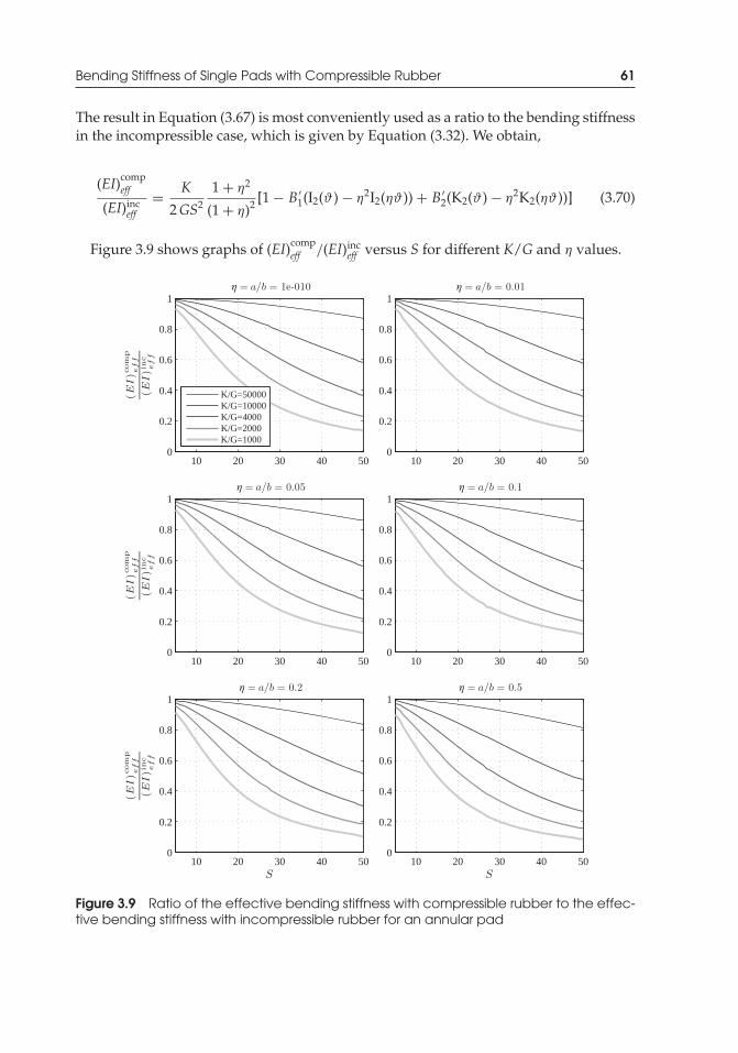
P1: TIX/XYZ P2: ABCJWST069-03 JWST069-Kelly-Style2 July 15, 2011 16:32 Printer Name: Yet to Come
Bending Stiffness of Single Pads with Compressible Rubber 61
The result in Equation (3.67) is most conveniently used as a ratio to the bending stiffnessin the incompressible case, which is given by Equation (3.32). We obtain,
(EI)compeff
(EI)inceff
= K
2GS2
1 + η2
(1 + η)2 [1 − B ′1(I2(ϑ) − η2I2(ηϑ)) + B ′
2(K2(ϑ) − η2K2(ηϑ))] (3.70)
Figure 3.9 shows graphs of (EI)compeff /(EI)inc
eff versus S for different K/G and η values.
10 20 30 40 500
0.2
0.4
0.6
0.8
1
(EI)co
mp
eff
(EI)in
ceff
η = a/b = 1e-010
K/G=50000K/G=10000K/G=4000K/G=2000K/G=1000
10 20 30 40 500
0.2
0.4
0.6
0.8
1η = a/b = 0.01
10 20 30 40 500
0.2
0.4
0.6
0.8
1
(EI)co
mp
eff
(EI)in
ceff
η = a/b = 0.05
10 20 30 40 500
0.2
0.4
0.6
0.8
1η = a/b = 0.1
10 20 30 40 500
0.2
0.4
0.6
0.8
1
S
(EI)co
mp
eff
(EI)in
ceff
η = a/b = 0.2
10 20 30 40 500
0.2
0.4
0.6
0.8
1
S
η = a/b = 0.5
Figure 3.9 Ratio of the effective bending stiffness with compressible rubber to the effec-tive bending stiffness with incompressible rubber for an annular pad
P1: TIX/XYZ P2: ABCJWST069-03 JWST069-Kelly-Style2 July 15, 2011 16:32 Printer Name: Yet to Come
62 Behavior of Multilayer Rubber Bearings under Bending
The analysis given in this chapter has focused on the bending stiffness for a widevariety of isolator shapes. The bending stiffness of a rubber isolator is an importantbearing property that must be available for design in estimating the buckling behavior ofthe isolator. It allows us to assess the response of the compressed bearing to an externallyapplied bending moment and is needed to estimate the influenc of the vertical load onthe horizontal stiffness of a bearing. In addition, when the isolator is subject to sheardeformation, a bending moment is generated by the unbalanced shear forces at the topand bottom of the bearing. These bending moments cause shear strains in the rubberthat are important for design. Also, the moments produce compressive stresses in theshims that can result in buckling. The bending stiffness analyses that were presentedin this chapter for many shapes of isolators and which include bulk-compressibilityeffects are entirely new and are essential for a complete analysis of the types of bearingsthat are used in current design practise, where very large shape-factor rubber layers arepreferred by the manufacturers.
P1: TIX/XYZ P2: ABCJWST069-04 JWST069-Kelly-Style2 July 27, 2011 11:34 Printer Name: Yet to Come
4Steel Stress in MultilayerRubber Bearings underCompression and Bending
The essential characteristic of the rubber isolator is the very large ratio of the verticalstiffness to the horizontal stiffness. This is produced by the reinforcing plates, which incurrent industry standard are thin steel plates called shims. The shims prevent lateralbulging of the rubber, but allow the rubber to shear freely. The vertical stiffness of thebearing can be several hundred times the horizontal stiffness. The steel reinforcementhas the effect of generating shear stresses in the rubber, and these stresses act on the steelplates to cause tensile stresses which, if they were to become large enough, could resultin failure of the steel shims through yielding or fracture. The external pressure on theisolator at which this might happen is an important design quantity, and it is thereforenecessary to be able to estimate these tensile stresses under the applied external load.
In this chapter, solutions are developed for the tensile stresses in the steel reinforcingshims of rubber isolators. The method makes use of generalized plane stress and usesa stress function approach, treating the shim as a thin plate with body forces generatedby surface shears on the top and bottom of the plate. It is shown that the pressurein the rubber acts as a potential for these body forces. Solutions are presented for thecase of rubber bearings with low and moderate shape factors, where it is acceptable toassume that the rubber is incompressible, and also for the more common case in currentpractice where the shape factor is so large that the assumption of incompressibilitycannot be made, and the effect of the bulk modulus of the rubber must be included.The stress state in the steel reinforcing plates is calculated for pure compression and for
The material in Sections 4.2 and 4.3 firs appeared in the article by Kelly, J. M. and Konstantinidis, D. (2009).“Steel Shim Stresses in Multilayer Bearings under Compression and Bending.” Journal of Mechanics of Materialsand Structures, 4(6), 1109–1125, DOI: 10.2140/jomms.2009.4.1109. Reproduced by permission of MathematicalSciences Publishers.
Mechanics of Rubber Bearings for Seismic and Vibration Isolation, First Edition. James M. Kelly and Dimitrios A. Konstantinidis.C© 2011 John Wiley & Sons, Ltd. Published 2011 by John Wiley & Sons, Ltd.
63
P1: TIX/XYZ P2: ABCJWST069-04 JWST069-Kelly-Style2 July 27, 2011 11:34 Printer Name: Yet to Come
64 Steel Stress in Multilayer Rubber Bearings under Compression and Bending
pure bending of the bearing. These two cases, separately and their combination, are thetypical situation in current practice. While a solution for the stress state in the shims ofa circular isolator, assuming incompressibility and under pure compression, has beenavailable using an analogy with the stresses in a rotating circular plate, the use of thestress function method is new (Kelly and Konstantinidis 2009a) and suggests a methodto extend the solutions to isolators with shapes other than circular.
In the later part of the chapter we look into the yielding of the steel shims, and weshow that the result for the pressure that causes full yielding throughout the steel shimin the incompressible case is a conservative estimate of the pressure to produce full yieldin the case of the larger-shape-factor isolator, for which the compressibility of the rubbermust be taken into account.
4.1 Review of the Compression and Bending of a Pad
In Chapters 2 and 3, the pure compression and pure bending of a single pad were inves-tigated, and the results important for the developments in this chapter are restated herefor convenience to the reader. The pressure solution for the case of a circular bearing ofradiusRwith incompressible rubber, which applies to low and moderate shape factors, is
p(r ) = 3Gεc
t2 (R2 − r2) (4.1)
The compressive load is then given by
P = 2π
∫ R
0p (r ) rdr = 3GεcπR4
2t2 (4.2)
and, with S = R/(2t) and A= πR2, the compression modulus, Ec = P/(Aεc), becomes
Ec = 6GS2 (4.3)
Under pure bending, the pressure solution for the circular pad with incompressiblerubber is
p(r ) = 3G2t2
α
t(r2 − R2)r cos θ (4.4)
It is useful to defin a bending strain εb, analogous to the compression strain εc, as
εb = α
tR (4.5)
Then Equation (4.4) becomes
p(r ) = 3Gεb
2Rt2 (r2 − R2) r cos θ = 6GS2εb
(r 2
R2 − 1)rR
cos θ (4.6)
P1: TIX/XYZ P2: ABCJWST069-04 JWST069-Kelly-Style2 July 27, 2011 11:34 Printer Name: Yet to Come
Steel Stresses in Circular Bearings with Incompressible Rubber 65
In the case of compressible rubber, which applies to bearings with larger shape factors,the pressure solution for a circular bearing under pure compression is
p(r ) = K εc
(1 − I0(λr )
I0(λR)
)(4.7)
where I0 is the zero-order modifie Bessel function of the firs kind. Integrating p overthe area of the pad gives P = K εc R2[1 − 2I1(λR)/(λRI0(λR))] where I1 is the modifieBessel function of the firs kind of order 1. The resulting expression for the compressionmodulus is
Ec = K(
1 − 2λR
I1(λR)I0(λR)
)(4.8)
where λR =√
12GR2/(Kt2) = √48G/K S.
For a circular pad with compressible rubber under pure bending, it was shown inChapter 3 that the pressure distribution takes the form
p(r ) = Kα
t
(RI1(λr )I1(λR)
− r)
cos θ = K εb
(I1(λr )I1(λR)
− rR
)cos θ (4.9)
4.2 Steel Stresses in Circular Bearings with Incompressible Rubber
The state of stress in a rubber layer, within a multilayer bearing under compression orbending, or a combination of the two, is assumed to be a state of pressure that wouldinduce a bulging of the rubber were it not restrained by the thin steel reinforcing shimsthat are bonded to the rubber (see Figure 1.4). The restraint of the rubber by the steelcauses shear stresses in the rubber which act on each side of the steel plate to inducetensile or compressive stresses in the plane of the plate. It is possible to solve for thesein-plane stresses using two-dimensional elasticity theory, assuming that the plate is ina state of generalized plane stress and that the surface shear stresses are equivalentto in-plane body forces. While it is possible to formulate the plane-stress problem foran arbitrarily shaped plate, we will consider only the circular bearing. We will use thenotations for the stresses and the stress function from Timoshenko and Goodier (1970).
In polar coordinates (r, θ ), the equations of equilibrium for the stresses in therubber are
∂σr
∂r+ 1r
∂τrθ
∂θ+ ∂τrz
∂z+ σr − σθ
r= 0
∂τrθ
∂r+ 1r
∂σθ
∂θ+ ∂τθz
∂z+ 2τrθ
r= 0
∂τrz
∂r+ 1r
∂τθz
∂θ+ ∂σz
∂z+ τrz
r= 0
(4.10)
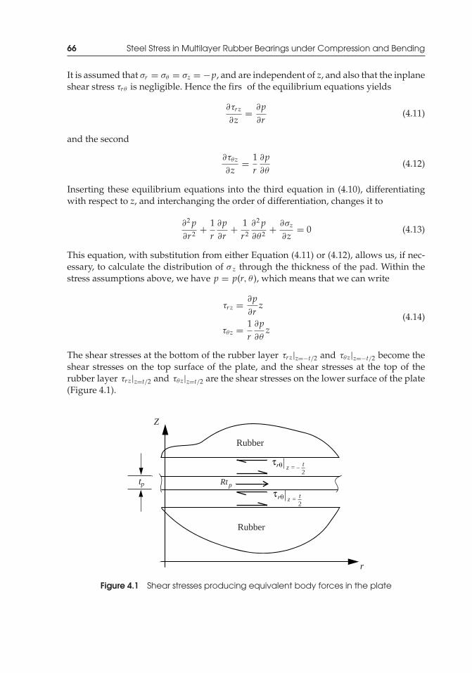
P1: TIX/XYZ P2: ABCJWST069-04 JWST069-Kelly-Style2 July 27, 2011 11:34 Printer Name: Yet to Come
66 Steel Stress in Multilayer Rubber Bearings under Compression and Bending
It is assumed that σr = σθ = σz = −p, and are independent of z, and also that the inplaneshear stress τrθ is negligible. Hence the firs of the equilibrium equations yields
∂τrz
∂z= ∂p
∂r(4.11)
and the second
∂τθz
∂z= 1r
∂p∂θ
(4.12)
Inserting these equilibrium equations into the third equation in (4.10), differentiatingwith respect to z, and interchanging the order of differentiation, changes it to
∂2 p∂r 2 + 1
r∂p∂r
+ 1r2
∂2 p∂θ 2 + ∂σz
∂z= 0 (4.13)
This equation, with substitution from either Equation (4.11) or (4.12), allows us, if nec-essary, to calculate the distribution of σ z through the thickness of the pad. Within thestress assumptions above, we have p = p(r, θ ), which means that we can write
τrz = ∂p∂rz
τθz = 1r
∂p∂θ
z(4.14)
The shear stresses at the bottom of the rubber layer τrz|z=−t/2 and τθz|z=−t/2 become theshear stresses on the top surface of the plate, and the shear stresses at the top of therubber layer τrz|z=t/2 and τθz|z=t/2 are the shear stresses on the lower surface of the plate(Figure 4.1).
r
Z
tp
Rubber
Rubber
z t2
=
z t2
= –
Rtp
Figure 4.1 Shear stresses producing equivalent body forces in the plate
P1: TIX/XYZ P2: ABCJWST069-04 JWST069-Kelly-Style2 July 27, 2011 11:34 Printer Name: Yet to Come
Steel Stresses in Circular Bearings with Incompressible Rubber 67
The internal stresses in the steel shims satisfy the equilibrium equations
∂σr
∂r+ 1r
∂τrθ
∂θ+ σr − σθ
r+ R = 0
∂τrθ
∂r+ 1r
∂σθ
∂θ+ 2τrθ
r+ S = 0
(4.15)
where R and S are the equivalent body forces per unit volume created by the surfaceshear stresses and are given by
tp R = τrz|z=−t/2 − τrz|z=t/2
tpS = τθz|z=−t/2 − τθz|z=t/2
(4.16)
where tp is the thickness of the steel shim, leading to
R = − ttp
∂p∂r
S = − ttp
1r
∂p∂θ
(4.17)
It follows that the pressure plays the role of a potential, V, for the body forces inthe form
V(r, θ ) = ttpp(r, θ ) (4.18)
with
R = −∂V∂r
and S = −1r
∂V∂θ
(4.19)
The equations of equilibrium for the plate then become
∂(σr − V)∂r
+ 1r
∂τrθ
∂θ+ (σr − V) − (σθ − V)
r= 0
∂τrθ
∂r+ 1r
∂(σθ − V)∂θ
+ 2τrθ
r= 0
(4.20)
P1: TIX/XYZ P2: ABCJWST069-04 JWST069-Kelly-Style2 July 27, 2011 11:34 Printer Name: Yet to Come
68 Steel Stress in Multilayer Rubber Bearings under Compression and Bending
These equations are satisfie by a stress function (r, θ ) for the stresses, such that
σr − V = 1r
∂
∂r+ 1r2
∂2
∂θ2
σθ − V = ∂2
∂r 2
τrθ = − ∂
∂r
(1r
∂
∂θ
)(4.21)
and under the assumption of plane stress, the equation for is
∇2∇2 + (1 − ν)∇2V = 0 (4.22)
where ν is the Poisson’s ratio of the steel. In the case of pure compression, the pres-sure satisfie
∇2 p = −12Gεc
t2 (4.23)
and for bending
∇2 p = 12Gεb
t2rR
cos θ (4.24)
4.2.1 Stress Function Solution for Pure Compression
The stress function for pure compression is given by the solution of
∇2∇2 + C = 0 (4.25)
where C is a constant having the value
C = −(1 − ν)12Gεc
tpt(4.26)
In this case the stress function depends only on r, and we look for a solution of that form.The result is (Timoshenko and Goodier 1970)
= Aln r + Br2 ln r + Cr2 + D− Cr4
64(4.27)
The resulting stresses are given by
σr − ttpp(r ) = A
r2 + B(1 + 2 ln r ) + 2C − 116Cr2
σθ − ttpp(r ) = − A
r2 + B(3 + 2 ln r ) + 2C − 316Cr2
(4.28)
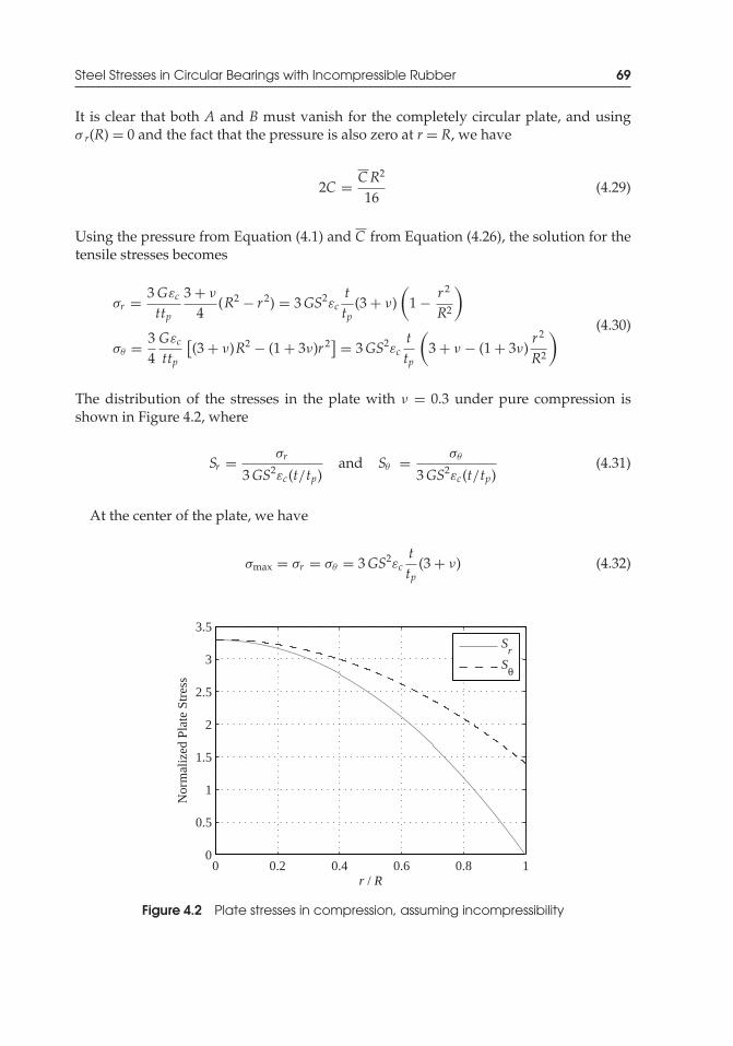
P1: TIX/XYZ P2: ABCJWST069-04 JWST069-Kelly-Style2 July 27, 2011 11:34 Printer Name: Yet to Come
Steel Stresses in Circular Bearings with Incompressible Rubber 69
It is clear that both A and B must vanish for the completely circular plate, and usingσ r(R) = 0 and the fact that the pressure is also zero at r = R, we have
2C = CR2
16(4.29)
Using the pressure from Equation (4.1) and C from Equation (4.26), the solution for thetensile stresses becomes
σr = 3Gεc
ttp
3 + ν
4(R2 − r2) = 3GS2εc
ttp
(3 + ν)(
1 − r2
R2
)
σθ = 34Gεc
ttp
[(3 + ν)R2 − (1 + 3ν)r 2] = 3GS2εc
ttp
(3 + ν − (1 + 3ν)
r2
R2
) (4.30)
The distribution of the stresses in the plate with ν = 0.3 under pure compression isshown in Figure 4.2, where
Sr = σr
3GS2εc(t/tp)and Sθ = σθ
3GS2εc(t/tp)(4.31)
At the center of the plate, we have
σmax = σr = σθ = 3GS2εcttp
(3 + ν) (4.32)
0 0.2 0.4 0.6 0.8 10
0.5
1
1.5
2
2.5
3
3.5
r / R
Nor
mal
ized
Pla
te S
tres
s
S
r
Sθ
Figure 4.2 Plate stresses in compression, assuming incompressibility

P1: TIX/XYZ P2: ABCJWST069-04 JWST069-Kelly-Style2 July 27, 2011 11:34 Printer Name: Yet to Come
70 Steel Stress in Multilayer Rubber Bearings under Compression and Bending
By expressing the maximum stresses in terms of the average pressure over the plate,pave, given by
pave = Ecεc = 6GS2εc (4.33)
we obtain
σmax
Pave= 3 + ν
2ttp
(4.34)
which can be used to determine the maximum pressure needed to cause yield in theshim at the center. It shows why, under normal circumstances, the stresses in the shimsdue to the pressure are not considered important. For example, if we have steel shims3-mm (0.118 in.) thick and 15-mm (0.591 in.) thick rubber layers, the stresses in the steeldue to a pressure of 7.0 MPa (1.0 ksi), which is standard, are only 58 MPa (8.4 ksi), wellbelow the yield level of the plate material. If the tension stress at the center is in fact theyield stress of the material σ o, then the average pressure to initiate yield is
pave = 23 + ν
tpt
σo (4.35)
This is only the start of yield, but the plate will experience further yielding as the pressureincreases. The zone of yielding will spread from the center to the outer radius so that thepressure can increase further until the entire plate has yielded, that is, until the region0 ≤ r ≤ R is fully plastic.
It is interesting to note that the problem in this case is the same as that for thestresses in a thin disk due to centrifugal forces. That solution was given in Timoshenkoand Goodier (1970) using an entirely different approach based on displacements, and,except for constants, is identical to this. Timoshenko and Goodier (1970) also provide thesolution for a circular plate of radius bwith a central hole of radius a, which for a≤ r≤ b is
σr = 34Gεc
ttp(3 + ν)
(b2 + a2 − a2b2
r2 − r2)
σθ = 34Gεc
ttp(3 + ν)
(b2 + a2 + a2b2
r2 − 1 + 3ν
3 + νr 2
) (4.36)
The maximum radial stress is at r = √ab, where
σr = 34Gεc
ttp(3 + ν)(b − a )2 (4.37)
and the maximum tangential stress is at the inner boundary, where
σθ = 34Gεc
ttp(3 + ν)
(b2 + 1 − ν
3 + νa2
)(4.38)
This is always larger than the maximum radial stress. When the radius a of the hole be-comes very small, the maximum tangential stress approaches a value twice as large as thecomplete circular plate. This is another example of a stress concentration at a small hole.
P1: TIX/XYZ P2: ABCJWST069-04 JWST069-Kelly-Style2 July 27, 2011 11:34 Printer Name: Yet to Come
Steel Stresses in Circular Bearings with Incompressible Rubber 71
4.2.2 Stress Function Solution for Pure Bending
For the case of pure bending on the pad, the equation for the stress function takesthe form
∇2∇2 + Cr cos θ = 0 (4.39)
where now
C = (1 − ν)12Gεb
Rttp(4.40)
We look for a solution of the form
(r, θ ) = f (r ) cos θ (4.41)
From Timoshenko and Goodier (1970), the ordinary differential equation for f is
d4 fdr 4 + 2
rd3 fdr3 − 3
r2
d2 fdr 2 + 3
r3
d fdr
− 3r4 f + Cr = 0 (4.42)
The solution is
f (r ) = Ar3 + Br
+ Cr + Dr ln r − Cr5
192(4.43)
The resulting stresses are
σr − ttpp =
(2Ar − 2B
r3 + Dr
)cos θ + R
σθ − ttpp =
(6Ar + 2B
r3 + Dr
)cos θ + S
τrθ =(
2Ar − 2Br3 + D
r
)sin θ + T
(4.44)
where
R =(
1r
∂
∂r+ 1r2
∂2
∂θ2
)(−Cr5
192cos θ
)= −Cr3
48cos θ
S = ∂2
∂r 2
(−Cr5
192cos θ
)= −5Cr3
48cos θ
T = − ∂
∂r
[1r
∂
∂θ
(−Cr5
192cos θ
)]= −Cr3
48sin θ
(4.45)
For the complete plate, 0 ≤ r ≤ R, both B and D must vanish, giving
σr = ttpp(r, θ ) + 2Ar cos θ − Cr3
48cos θ (4.46)
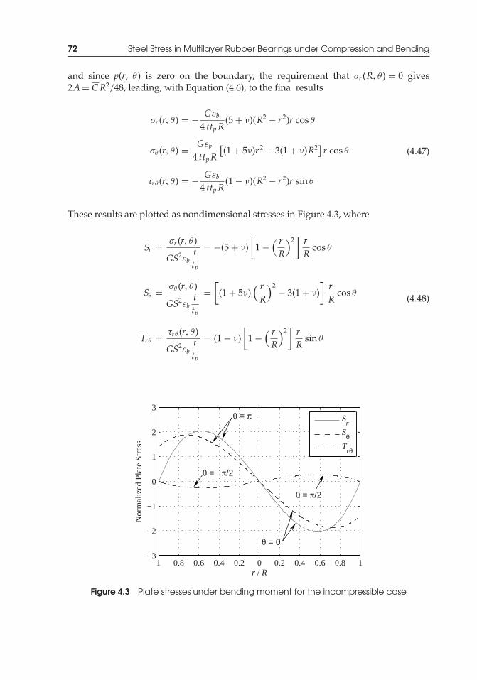
P1: TIX/XYZ P2: ABCJWST069-04 JWST069-Kelly-Style2 July 27, 2011 11:34 Printer Name: Yet to Come
72 Steel Stress in Multilayer Rubber Bearings under Compression and Bending
and since p(r, θ ) is zero on the boundary, the requirement that σr (R, θ ) = 0 gives2A= CR2/48, leading, with Equation (4.6), to the fina results
σr (r, θ ) = − Gεb
4 ttp R(5 + ν)(R2 − r 2)r cos θ
σθ (r, θ ) = Gεb
4 ttp R[(1 + 5ν)r2 − 3(1 + ν)R2] r cos θ
τrθ (r, θ ) = − Gεb
4 ttp R(1 − ν)(R2 − r 2)r sin θ
(4.47)
These results are plotted as nondimensional stresses in Figure 4.3, where
Sr = σr (r, θ )
GS2εbttp
= −(5 + ν)[
1 −( rR
)2]rR
cos θ
Sθ = σθ (r, θ )
GS2εbttp
=[
(1 + 5ν)( rR
)2− 3(1 + ν)
]rR
cos θ
Trθ = τrθ (r, θ )
GS2εbttp
= (1 − ν)[
1 −( rR
)2]rR
sin θ
(4.48)
1 0.8 0.6 0.4 0.2 0 0.2 0.4 0.6 0.8 1−3
−2
−1
0
1
2
3θ = π
θ = 0
θ = π/2
r / R
Nor
mal
ized
Pla
te S
tres
s
θ = −π/2
Sr
SθT
rθ
Figure 4.3 Plate stresses under bending moment for the incompressible case
P1: TIX/XYZ P2: ABCJWST069-04 JWST069-Kelly-Style2 July 27, 2011 11:34 Printer Name: Yet to Come
Steel Stresses in Circular Bearings with Compressible Rubber 73
4.3 Steel Stresses in Circular Bearings with Compressible Rubber
4.3.1 Stress Function Solution for Pure Compression
The tension stresses in the steel reinforcing plates can be calculated in the same way asbefore by using the stress function method. The equation for the stress function remainsthe same, ∇2∇2 + (1 − ν)∇2V = 0, and the definitio of the potentialV(r, θ ) is the same,V = (t/tp)p(r, θ ), but the pressure now satisfie the equation
∇2 p − 12GKt2
p = −12Gεc
t2 (4.49)
Thus the stress function now must satisfy the equation
∇2∇2 + (1 − ν)ttp
12Gt2
( pK
− εc
)= 0 (4.50)
With p given by Equation (4.7), we have
∇2∇2 − (1 − ν)ttp
12Gt2
I0(λr )I0(λR)
εc = 0 (4.51)
The solution for pure compression is rotationally symmetric, and the complementarypart of the solution remains the same, but it is necessary to determine the partic-ular integral that corresponds to the term I0(λr ). To develop this, we recall that inradial symmetry,
∇2∇2( f ) = 1r
ddr
(r
ddr
(1r
ddr
(r
d fdr
)))(4.52)
By taking f = I0(λr ), changing the variable to x = λr , and recalling that x so define isdimensionless and that λ is a reciprocal length, we have ∇2∇2|r = (1/λ4)∇2∇2|x.
Thus, we have successively
1x
ddx
(x
ddx
(1x
ddx
(x
d fdx
)))= I0(x)
xd
dx
(1x
ddx
(x
d fdx
))=
∫xI0(x) dx = xI1(x)
1x
ddx
(x
d fdx
)=
∫I1(x) dx = I0(x)
xd fdx
=∫xI0(x) dx = xI1(x)
f = I0(x)
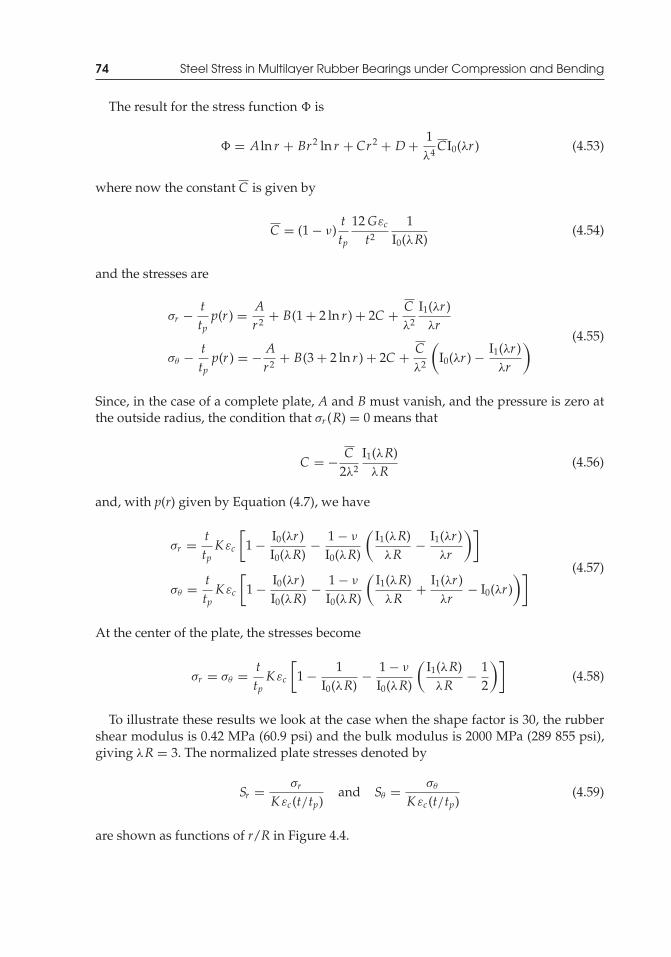
P1: TIX/XYZ P2: ABCJWST069-04 JWST069-Kelly-Style2 July 27, 2011 11:34 Printer Name: Yet to Come
74 Steel Stress in Multilayer Rubber Bearings under Compression and Bending
The result for the stress function is
= Aln r + Br2 ln r + Cr2 + D+ 1λ4CI0(λr ) (4.53)
where now the constant C is given by
C = (1 − ν)ttp
12Gεc
t2
1I0(λR)
(4.54)
and the stresses are
σr − ttpp(r ) = A
r2 + B(1 + 2 ln r ) + 2C + Cλ2
I1(λr )λr
σθ − ttpp(r ) = − A
r2 + B(3 + 2 ln r ) + 2C + Cλ2
(I0(λr ) − I1(λr )
λr
) (4.55)
Since, in the case of a complete plate, A and B must vanish, and the pressure is zero atthe outside radius, the condition that σr (R) = 0 means that
C = − C2λ2
I1(λR)λR
(4.56)
and, with p(r) given by Equation (4.7), we have
σr = ttpK εc
[1 − I0(λr )
I0(λR)− 1 − ν
I0(λR)
(I1(λR)
λR− I1(λr )
λr
)]
σθ = ttpK εc
[1 − I0(λr )
I0(λR)− 1 − ν
I0(λR)
(I1(λR)
λR+ I1(λr )
λr− I0(λr )
)] (4.57)
At the center of the plate, the stresses become
σr = σθ = ttpK εc
[1 − 1
I0(λR)− 1 − ν
I0(λR)
(I1(λR)
λR− 1
2
)](4.58)
To illustrate these results we look at the case when the shape factor is 30, the rubbershear modulus is 0.42 MPa (60.9 psi) and the bulk modulus is 2000 MPa (289 855 psi),giving λR = 3. The normalized plate stresses denoted by
Sr = σr
K εc(t/tp)and Sθ = σθ
K εc(t/tp)(4.59)
are shown as functions of r/R in Figure 4.4.
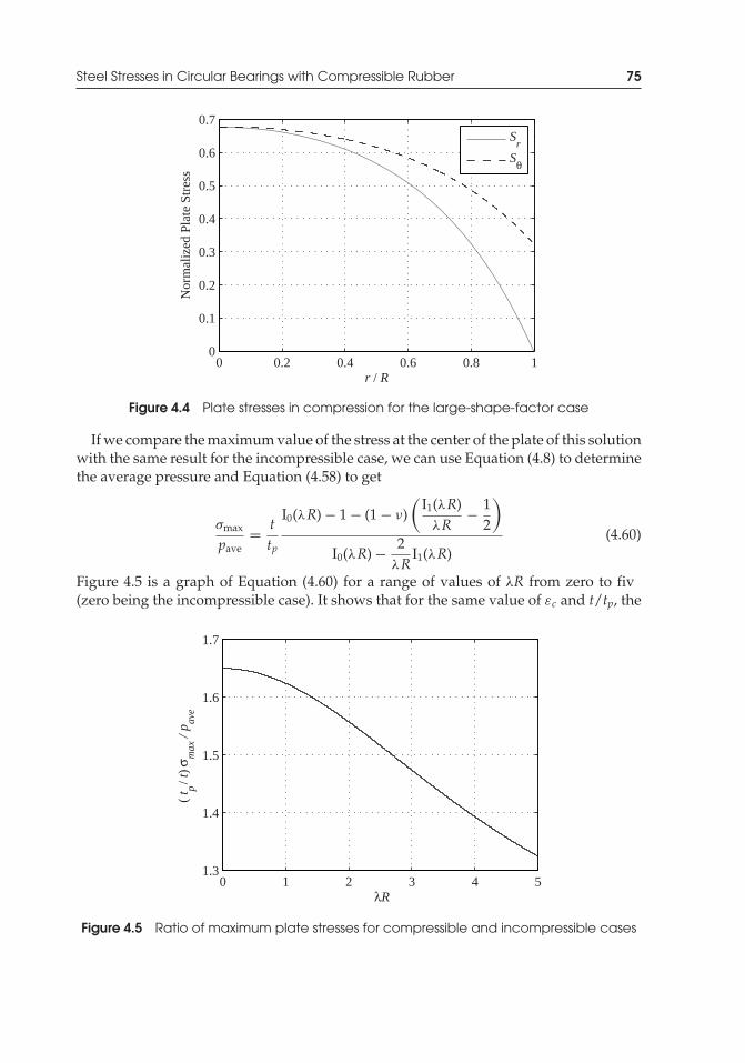
P1: TIX/XYZ P2: ABCJWST069-04 JWST069-Kelly-Style2 July 27, 2011 11:34 Printer Name: Yet to Come
Steel Stresses in Circular Bearings with Compressible Rubber 75
0 0.2 0.4 0.6 0.8 10
0.1
0.2
0.3
0.4
0.5
0.6
0.7
r / R
Nor
mal
ized
Pla
te S
tres
s
S
r
Sθ
Figure 4.4 Plate stresses in compression for the large-shape-factor case
If we compare the maximum value of the stress at the center of the plate of this solutionwith the same result for the incompressible case, we can use Equation (4.8) to determinethe average pressure and Equation (4.58) to get
σmax
pave= ttp
I0(λR) − 1 − (1 − ν)(
I1(λR)λR
− 12
)
I0(λR) − 2λR
I1(λR)(4.60)
Figure 4.5 is a graph of Equation (4.60) for a range of values of λR from zero to fiv(zero being the incompressible case). It shows that for the same value of εc and t/tp, the
0 1 2 3 4 51.3
1.4
1.5
1.6
1.7
λR
( t
/ t)
pσ m
ax /
p ave
Figure 4.5 Ratio of maximum plate stresses for compressible and incompressible cases
P1: TIX/XYZ P2: ABCJWST069-04 JWST069-Kelly-Style2 July 27, 2011 11:34 Printer Name: Yet to Come
76 Steel Stress in Multilayer Rubber Bearings under Compression and Bending
peak stresses get smaller as compressibility increases. This implies that the result for theincompressible computation is a conservative estimate of the stresses in the large-shape-factor case, which, if it can be used, greatly simplifie the prediction of the maximumvalue of the tension stress.
4.3.2 Stress Function Solution for Pure Bending
For a circular pad under pure bending with an angle of rotation α between the shims(see Figure 3.1), Equations (4.9) and (4.22) give the equation to be solved for thestress function
∇2∇2 + (1 − ν)ttp
12Gεb
t2I1(λr )I1(λR)
cos θ = 0 (4.61)
We look for a solution of the form
(r, θ ) = f (r ) cos θ (4.62)
Substitution into Equation (4.61) results in the ordinary differential equation for f
d4 fdr 4 + 2
rd3 fdr 3 − 3
r2
d2 fdr2 + 3
r3
d fdr
− 3r4 f + CI1(λr ) = 0 (4.63)
where
C = (1 − ν)ttp
12Gεb
t2
1I1(λR)
(4.64)
The complementary part of the solution is
f (r ) = Ar3 + Br
+ Cr + Dr ln r (4.65)
and the particular integral can be shown (after considerable algebraic manipulation) tobe −(C/λ4)I1(λr ).
The resulting stresses are
σr − ttpp =
(2Ar − 2B
r3 + Dr
)cos θ + R
σθ − ttpp =
(6Ar + 2B
r3 + Dr
)cos θ + S
τrθ =(
2Ar − 2Br3 + D
r
)sin θ + T
(4.66)
P1: TIX/XYZ P2: ABCJWST069-04 JWST069-Kelly-Style2 July 27, 2011 11:34 Printer Name: Yet to Come
Steel Stresses in Circular Bearings with Compressible Rubber 77
where
R =(
1r
∂
∂r+ 1r2
∂2
∂θ2
)(− (CI1(λr ) cos θ )
λ4
)= 2I1(λr ) − I0(λr )λr
λ2r2
Cλ2 cos θ
S = ∂2
∂r2
(−
(CI1(λr ) cos θ
)λ4
)= I0(λr )λr − I1(λr )
(2 + λ2r2
)λ2r2
Cλ2 cos θ
T = − ∂
∂r
(1r
∂
∂θ
(−
(CI1 (λr ) cos θ
)λ4
))= 2I1(λr ) − I0(λr )λr
λ2r2
Cλ2 sin θ
(4.67)
For the complete plate, 0 ≤ r ≤ R, both B and D must vanish and σr (R, θ ) = 0,giving
A= 12 R
I0 (λR) λR− 2I1 (λR)λ2R2
Cλ2 (4.68)
Substituting for p(r, θ ) from Equation (4.9) and C from Equation (4.64), and making useof λ2 = 12G/(Kt2) leads to
σr = K εbttp
[I1(λr )I1(λR)
− rR
+ 1 − ν
I1(λR)
(I0 (λR) λR− 2I1 (λR)
λ2R2
rR
− I0 (λr ) λr − 2I1 (λr )λ2r2
)]cos θ
σθ = K εbttp
[I1 (λr )I1 (λR)
− rR
+ 1 − ν
I1 (λR)
(3
I0 (λR) λR− 2I1 (λR)λ2R2
rR
+ I0 (λr ) λr − I1 (λr )(λ2r2 + 2
)λ2r2
)]cos θ
τrθ = K εbttp
1 − ν
I1 (λR)
(I0 (λR) λR− 2I1 (λR)
λ2R2
rR
− I0 (λr ) λr − 2I1 (λr )λ2r2
)sin θ
(4.69)
These results are plotted in Figure 4.6 for the case when λR = 3.
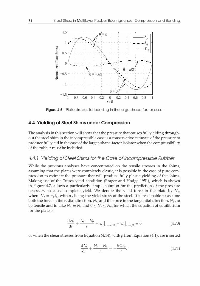
P1: TIX/XYZ P2: ABCJWST069-04 JWST069-Kelly-Style2 July 27, 2011 11:34 Printer Name: Yet to Come
78 Steel Stress in Multilayer Rubber Bearings under Compression and Bending
1 0.8 0.6 0.4 0.2 0 0.2 0.4 0.6 0.8 1−1.5
−1
−0.5
0
0.5
1
1.5 θ = π
θ = 0
θ = −π/2
r / R
Nor
mal
ized
Pla
te S
tres
s
θ = π/2
Sr
SθT
rθ
Figure 4.6 Plate stresses for bending in the large-shape-factor case
4.4 Yielding of Steel Shims under Compression
The analysis in this section will show that the pressure that causes full yielding through-out the steel shim in the incompressible case is a conservative estimate of the pressure toproduce full yield in the case of the larger-shape-factor isolator when the compressibilityof the rubber must be included.
4.4.1 Yielding of Steel Shims for the Case of Incompressible Rubber
While the previous analyses have concentrated on the tensile stresses in the shims,assuming that the plates were completely elastic, it is possible in the case of pure com-pression to estimate the pressure that will produce fully plastic yielding of the shims.Making use of the Tresca yield condition (Prager and Hodge 1951), which is shownin Figure 4.7, allows a particularly simple solution for the prediction of the pressurenecessary to cause complete yield. We denote the yield force in the plate by No,where No = σ otp, with σ o being the yield stress of the steel. It is reasonable to assumeboth the force in the radial direction, Nr, and the force in the tangential direction, Nθ , tobe tensile and to take Nθ = No and 0 ≤ Nr ≤ No, for which the equation of equilibriumfor the plate is
dNrdr
+ Nr − Nθ
r+ τrz
∣∣z=−t/2 − τrz
∣∣z= t/2 = 0 (4.70)
or when the shear stresses from Equation (4.14), with p from Equation (4.1), are inserted
dNrdr
+ Nr − Nθ
r= −6Gεc
tr (4.71)
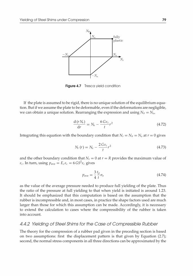
P1: TIX/XYZ P2: ABCJWST069-04 JWST069-Kelly-Style2 July 27, 2011 11:34 Printer Name: Yet to Come
Yielding of Steel Shims under Compression 79
No−No
No
−No
Nr
Nθ
fullyplastic
Figure 4.7 Tresca yield condition
If the plate is assumed to be rigid, there is no unique solution of the equilibrium equa-tion. But if we assume the plate to be deformable, even if the deformations are negligible,we can obtain a unique solution. Rearranging the expression and using Nθ = No,
d (rNr )dr
= No − 6Gεc
tr 2 (4.72)
Integrating this equation with the boundary condition that Nr = Nθ = No at r = 0 gives
Nr (r ) = No − 2Gεc
tr 2 (4.73)
and the other boundary condition that Nr = 0 at r = R provides the maximum value ofεc. In turn, using pave = Ecεc = 6GS2εc gives
pave = 34tpt
σo (4.74)
as the value of the average pressure needed to produce full yielding of the plate. Thusthe ratio of the pressure at full yielding to that when yield is initiated is around 1.23.It should be emphasized that this computation is based on the assumption that therubber is incompressible and, in most cases, in practice the shape factors used are muchlarger than those for which this assumption can be made. Accordingly, it is necessaryto extend the calculation to cases where the compressibility of the rubber is takeninto account.
4.4.2 Yielding of Steel Shims for the Case of Compressible Rubber
The theory for the compression of a rubber pad given in the preceding section is basedon two assumptions: first the displacement pattern is that given by Equation (2.7);second, the normal stress components in all three directions can be approximated by the
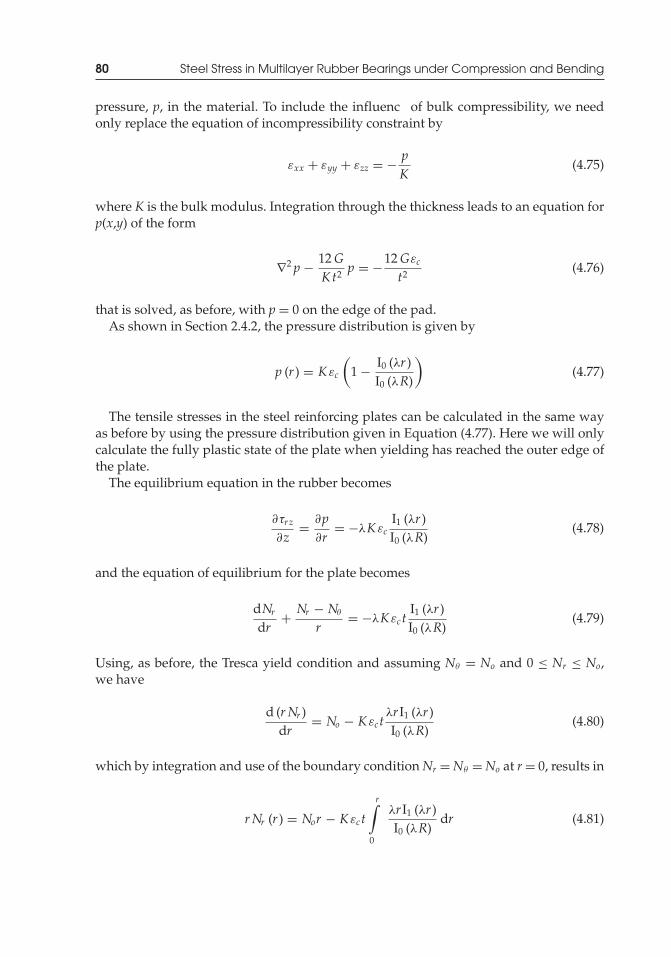
P1: TIX/XYZ P2: ABCJWST069-04 JWST069-Kelly-Style2 July 27, 2011 11:34 Printer Name: Yet to Come
80 Steel Stress in Multilayer Rubber Bearings under Compression and Bending
pressure, p, in the material. To include the influenc of bulk compressibility, we needonly replace the equation of incompressibility constraint by
εxx + εyy + εzz = − pK
(4.75)
where K is the bulk modulus. Integration through the thickness leads to an equation forp(x,y) of the form
∇2 p − 12GKt2 p = −12Gεc
t2 (4.76)
that is solved, as before, with p = 0 on the edge of the pad.As shown in Section 2.4.2, the pressure distribution is given by
p (r ) = K εc
(1 − I0 (λr )
I0 (λR)
)(4.77)
The tensile stresses in the steel reinforcing plates can be calculated in the same wayas before by using the pressure distribution given in Equation (4.77). Here we will onlycalculate the fully plastic state of the plate when yielding has reached the outer edge ofthe plate.
The equilibrium equation in the rubber becomes
∂τrz
∂z= ∂p
∂r= −λK εc
I1 (λr )I0 (λR)
(4.78)
and the equation of equilibrium for the plate becomes
dNrdr
+ Nr − Nθ
r= −λK εc t
I1 (λr )I0 (λR)
(4.79)
Using, as before, the Tresca yield condition and assuming Nθ = No and 0 ≤ Nr ≤ No,we have
d (rNr )dr
= No − K εctλr I1 (λr )I0 (λR)
(4.80)
which by integration and use of the boundary condition Nr =Nθ =No at r= 0, results in
rNr (r ) = Nor − K εc t
r∫0
λr I1 (λr )I0 (λR)
dr (4.81)
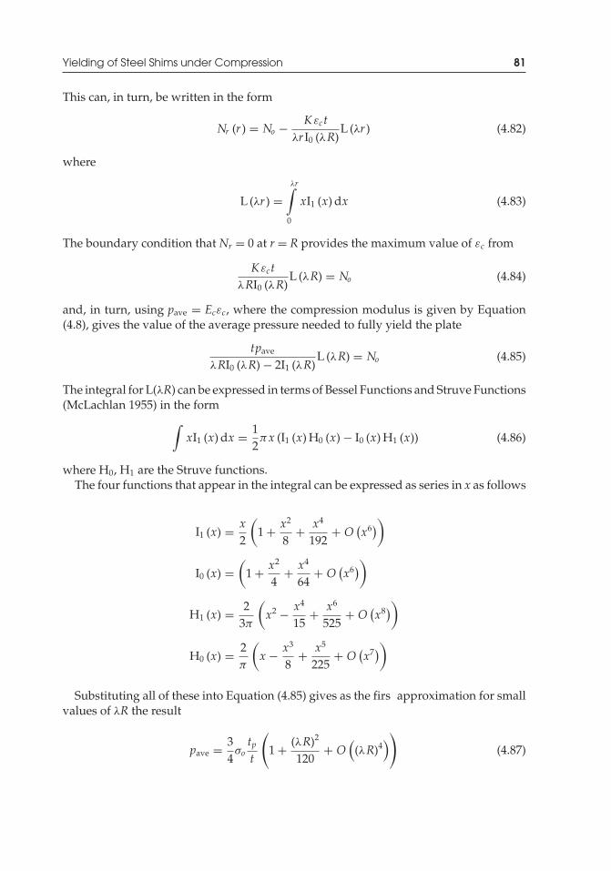
P1: TIX/XYZ P2: ABCJWST069-04 JWST069-Kelly-Style2 July 27, 2011 11:34 Printer Name: Yet to Come
Yielding of Steel Shims under Compression 81
This can, in turn, be written in the form
Nr (r ) = No − K εc tλr I0 (λR)
L (λr ) (4.82)
where
L (λr ) =λr∫
0
xI1 (x) dx (4.83)
The boundary condition that Nr = 0 at r = R provides the maximum value of εc from
K εctλRI0 (λR)
L (λR) = No (4.84)
and, in turn, using pave = Ecεc, where the compression modulus is given by Equation(4.8), gives the value of the average pressure needed to fully yield the plate
tpave
λRI0 (λR) − 2I1 (λR)L (λR) = No (4.85)
The integral for L(λR) can be expressed in terms of Bessel Functions and Struve Functions(McLachlan 1955) in the form
∫xI1 (x) dx = 1
2πx (I1 (x) H0 (x) − I0 (x) H1 (x)) (4.86)
where H0, H1 are the Struve functions.The four functions that appear in the integral can be expressed as series in x as follows
I1 (x) = x2
(1 + x2
8+ x4
192+ O
(x6))
I0 (x) =(
1 + x2
4+ x4
64+ O
(x6))
H1 (x) = 23π
(x2 − x4
15+ x6
525+ O
(x8))
H0 (x) = 2π
(x − x3
8+ x5
225+ O
(x7))
Substituting all of these into Equation (4.85) gives as the firs approximation for smallvalues of λR the result
pave = 34σotpt
(1 + (λR)2
120+ O
((λR)4
))(4.87)
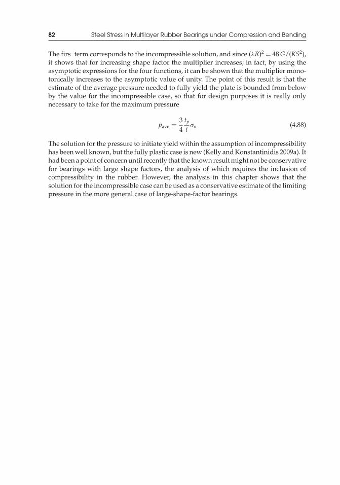
P1: TIX/XYZ P2: ABCJWST069-04 JWST069-Kelly-Style2 July 27, 2011 11:34 Printer Name: Yet to Come
82 Steel Stress in Multilayer Rubber Bearings under Compression and Bending
The firs term corresponds to the incompressible solution, and since (λR)2 = 48G/(KS2),it shows that for increasing shape factor the multiplier increases; in fact, by using theasymptotic expressions for the four functions, it can be shown that the multiplier mono-tonically increases to the asymptotic value of unity. The point of this result is that theestimate of the average pressure needed to fully yield the plate is bounded from belowby the value for the incompressible case, so that for design purposes it is really onlynecessary to take for the maximum pressure
pave = 34tpt
σo (4.88)
The solution for the pressure to initiate yield within the assumption of incompressibilityhas been well known, but the fully plastic case is new (Kelly and Konstantinidis 2009a). Ithad been a point of concern until recently that the known result might not be conservativefor bearings with large shape factors, the analysis of which requires the inclusion ofcompressibility in the rubber. However, the analysis in this chapter shows that thesolution for the incompressible case can be used as a conservative estimate of the limitingpressure in the more general case of large-shape-factor bearings.
P1: TIX/XYZ P2: ABCJWST069-05 JWST069-Kelly-Style2 July 15, 2011 14:38 Printer Name: Yet to Come
5Buckling Behavior ofMultilayer Rubber Isolators
5.1 Stability Analysis of Bearings
A multilayered rubber bearing can be susceptible to a buckling type of instability similarto that of an ordinary column, but dominated by the low-shear stiffness of a bearing. Theprevious analysis of the overall deformation of a single pad can be used in a bucklinganalysis that treats the bearing as a continuous composite system. This analysis considersthe bearing to be a beam, and the deformation is assumed to be such that plane sectionsnormal to the undeformed central axis remain plane, but not necessarily normal to thedeformed axis.
The theory for the buckling of isolation bearings is an outgrowth of work by Haringxin 1947 on the mechanical characteristics of helical steel springs and rubber rods used forvibration mountings. This work was published in a series of reports, the third of which(Haringx 1949) covers the stability of solid rubber rods. The Haringx theory was laterapplied by Gent (1964) to the problem of the stability of multilayered rubber compressionsprings, and it is this application that forms the basis for the theory given here.
The deformation pattern, shown in Figure 5.1, is define by two quantities: v(x) isthe displacement of the middle surface of the bearing, and ψ(x) is the rotation of aface originally normal to the undeformed axis. The overall shear deformation, γ , isthe difference between the rotation of the horizontal axis, v′(x), and the rotation of thenormal face, ψ (i.e., γ = v′ − ψ). Figure 5.2 shows the internal and external forces on thebearing in the deformed position. The shear force, V, and the axial force, N, are shownparallel and perpendicular, respectively, to the rotated face. The end loads, includingthe axial load, P, are define by a lateral reaction, H0, and bending moment, M0, whichmay be specifie or unknown, depending on the problem.
The internal shear force, V, is related to the shear deformation through
V = GAS(v′ − ψ)
Mechanics of Rubber Bearings for Seismic and Vibration Isolation, First Edition. James M. Kelly and Dimitrios A. Konstantinidis.C© 2011 John Wiley & Sons, Ltd. Published 2011 by John Wiley & Sons, Ltd.
83
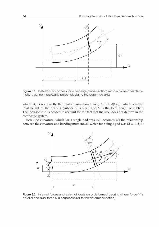
P1: TIX/XYZ P2: ABCJWST069-05 JWST069-Kelly-Style2 July 15, 2011 14:38 Printer Name: Yet to Come
84 Buckling Behavior of Multilayer Rubber Isolators
Figure 5.1 Deformation pattern for a bearing (plane sections remain plane after defor-mation, but not necessarily perpendicular to the deformed axis)
where AS is not exactly the total cross-sectional area, A, but A(h/tr ), where h is thetotal height of the bearing (rubber plus steel) and tr is the total height of rubber.The increase in A is needed to account for the fact that the steel does not deform in thecomposite system.
Here, the curvature, which for a single pad was α/t, becomes ψ ′; the relationshipbetween the curvature and bending moment,M, which for a single pad was EI = Ec I/3,
Figure 5.2 Internal forces and external loads on a deformed bearing (shear force V isparallel and axial force N is perpendicular to the deformed section)
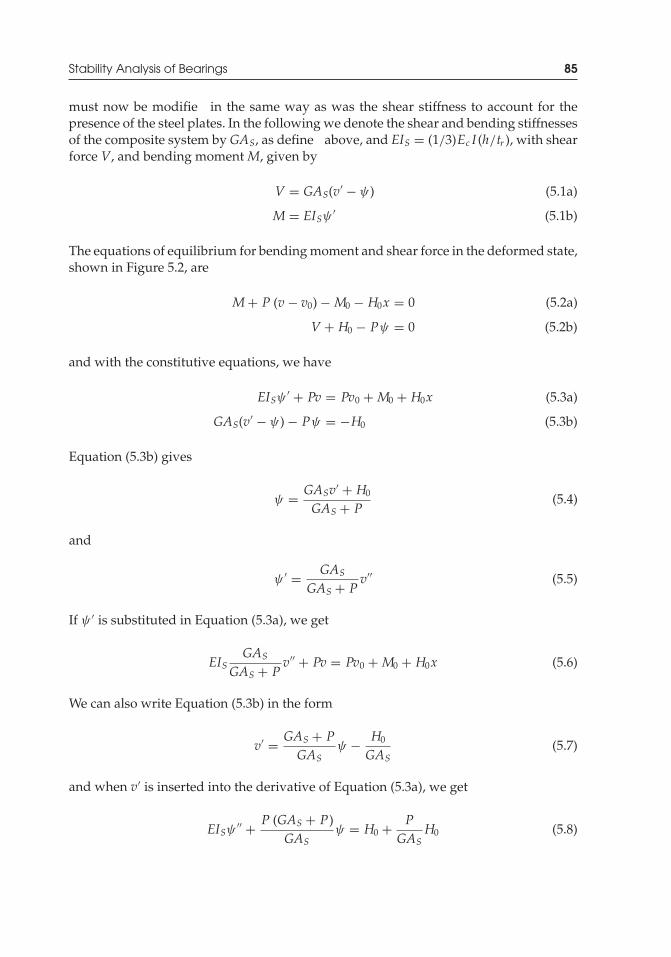
P1: TIX/XYZ P2: ABCJWST069-05 JWST069-Kelly-Style2 July 15, 2011 14:38 Printer Name: Yet to Come
Stability Analysis of Bearings 85
must now be modifie in the same way as was the shear stiffness to account for thepresence of the steel plates. In the following we denote the shear and bending stiffnessesof the composite system by GAS, as define above, and EIS = (1/3)Ec I (h/tr ), with shearforce V, and bending moment M, given by
V = GAS(v′ − ψ) (5.1a)
M = EISψ ′ (5.1b)
The equations of equilibrium for bending moment and shear force in the deformed state,shown in Figure 5.2, are
M+ P (v − v0) − M0 − H0x = 0 (5.2a)
V + H0 − Pψ = 0 (5.2b)
and with the constitutive equations, we have
EISψ ′ + Pv = Pv0 + M0 + H0x (5.3a)
GAS(v′ − ψ) − Pψ = −H0 (5.3b)
Equation (5.3b) gives
ψ = GASv′ + H0
GAS + P(5.4)
and
ψ ′ = GAS
GAS + Pv′′ (5.5)
If ψ ′ is substituted in Equation (5.3a), we get
EISGAS
GAS + Pv′′ + Pv = Pv0 + M0 + H0x (5.6)
We can also write Equation (5.3b) in the form
v′ = GAS + PGAS
ψ − H0
GAS(5.7)
and when v′ is inserted into the derivative of Equation (5.3a), we get
EISψ ′′ + P (GAS + P)GAS
ψ = H0 + PGAS
H0 (5.8)
P1: TIX/XYZ P2: ABCJWST069-05 JWST069-Kelly-Style2 July 15, 2011 14:38 Printer Name: Yet to Come
86 Buckling Behavior of Multilayer Rubber Isolators
or
EISGAS
GAS + Pψ ′′ + Pψ = H0 (5.9)
Thus, the two equations to be solved for the two kinematic variables, v and ψ , are
EISGAS
GAS + Pv′′ + Pv = Pv0 + M0 + H0x (5.10a)
EISGAS
GAS + Pψ ′′ + Pψ = H0 (5.10b)
It is useful to defin two parameters α and β as
α2 = P (GAS + P)EISGAS
and β = GAS
GAS + P(5.11)
The solutions for the two differential equations in Equations (5.10a) and (5.10b) are
v = Acos(αx) + B sin(αx) + v0 + M0
P+ H0
Px
ψ = C cos(αx) + D sin(αx) + H0
P
(5.12)
The constantsA, B,C,D are not independent, but are interrelated through Equation (5.7),which can be written in the form
v′ = 1β
ψ − H0
GAS(5.13)
and by substitution of Equation (5.12), leads to
− αAsin(αx) + αB cos(αx) + H0
P= 1
βC sin(αx) + 1
βD sin(αx) + 1
β
H0
P− H0
GAS(5.14)
giving the relationship between the constants as
C = αβB and D = −αβA (5.15)
The most general form of solution of Equations (5.10a) and (5.10b) becomes
v = Acos(αx) + B sin(αx) + v0 + M0
P+ H0
Px (5.16a)
ψ = αβB cos(αx) − αβAsin(αx) + H0
P(5.16b)

P1: TIX/XYZ P2: ABCJWST069-05 JWST069-Kelly-Style2 July 15, 2011 14:38 Printer Name: Yet to Come
Stability Analysis of Bearings 87
Figure 5.3 Boundary conditions for an isolation bearing under a vertical load P (thebearing buckles with no lateral force constraint but is prevented from rotating ateach end)
We now turn our attention to the specifi example of a bearing in an isolation system.As shown in Figure 5.3, the bearing is constrained against displacement at the bottom,rotation at the top and bottom, and is free to move laterally at the top. Setting x = 0 atthe bottom of the bearing and x = h at the top, we have
v(0) = 0, ψ(0) = 0, ψ(h) = 0, H0 = 0 (5.17)
thus Equation (5.16a) gives
A+ M0
P= 0 (5.18)
and Equation (5.16b) yields
ψ(0) = αβB = 0
ψ(h) = −αβAsin(αh) = 0(5.19)
Therefore, αh = π , and the general solution becomes
v(x) = 12δ(
1 − cos(πxh
))
ψ(x) = 12αβδ sin
(πxh
) (5.20)
and M0 = Pδ/2, where δ = v(h).
P1: TIX/XYZ P2: ABCJWST069-05 JWST069-Kelly-Style2 July 15, 2011 14:38 Printer Name: Yet to Come
88 Buckling Behavior of Multilayer Rubber Isolators
The result αh = π means
α2 = π2
h2 (5.21)
If we substitute the definitio of α2 from Equation (5.11), we get
P (GAS + P)GAS
= π2EISh2 = PE (5.22)
where PE is the Euler load for the standard column. If we denote GAS = PS, the aboveequation for the critical load, P, becomes
P2 + PSP − PSPE = 0 (5.23)
from which the critical load, Pcrit, is given by
Pcrit =−PS +
√P2S + 4PSPE
2(5.24)
If we now assume that PS ≈ GA and
PE ≈ π2
h2
13
6GS2 I ≈ GA(
2π2S2 IAh2
)(5.25)
then, for most types of bearings where S is 5 or greater, PE � PS, the critical load can beapproximated by
Pcrit =√PSPE (5.26)
Using this expression and recalling that
PS = GAhtr
PE = π2
h2
13Ec I
htr
(5.27)
we have
Pcrit =√(
GAhtr
) (π2
h2
13
6GS2Ar 2 htr
)
=√
2πGASrtr
(5.28)
P1: TIX/XYZ P2: ABCJWST069-05 JWST069-Kelly-Style2 July 15, 2011 14:38 Printer Name: Yet to Come
Stability Analysis of Bearings 89
where r is the radius of gyration, which is r = √I/A= a/(2
√3) for a square bearing
with side dimension a, and �/4 for a circular bearing with diameter �.The critical pressure, pcrit = Pcrit/A, can be expressed in terms of S and the quantity
S2, referred to as the aspect ratio or the second shape factor, define by
S2 = �
trfor a circular bearing (5.29a)
S2 = atr
for a square bearing (5.29b)
Thus
pcritG
= π
2√
2SS2 for a circular bearing (5.30a)
pcritG
= π√6SS2 for a square bearing (5.30b)
In actual design, the load carried by a bearing (say, W) will be less than the criticalload, and neglecting the effect of the vertical load on the horizontal stiffness, KH , of thebearing, this is given by KH = GA/tr , which in turn is related to the horizontal frequency,ωH , through
ω2H = KH
Wg (5.31)
Thus, the safety factor, S.F., against buckling, which is define by S.F. = Pcrit/W, becomes
S.F. =√
2πSω2Hr
g(5.32)
All other things being equal, the safety factor increases with shape factor, S, frequency,ωH , or bearing size (either a or �).
The bearing size will, of course, depend on the carried load. If the pressure, p = W/A,is specified then
r = 12√
π
(Wp
)1/2
for a circular bearing (5.33a)
r = 1
2√
3
(Wp
)1/2
for a square bearing (5.33b)
If the pressure is fixed the safety factor will diminish as W1/2, leading to the unexpectedresult that buckling can become a problem for bearings that are lightly loaded.
P1: TIX/XYZ P2: ABCJWST069-05 JWST069-Kelly-Style2 July 15, 2011 14:38 Printer Name: Yet to Come
90 Buckling Behavior of Multilayer Rubber Isolators
To get a feeling for the magnitude of the quantities involved, suppose that the safetyfactor must be at least three, the shape factor, S, is 10, and the frequency is π rad/s(2.0 s period), all of which are typical values. In this case, r must be at least
r = 3 · 9810√2 · π · 10 · π2
= 67.01 mm (2.64 in)
If the bearing is circular, then � = 268 mm (10.6 in). This minimum dimension isindependent of the carried load or the pressure, but if the pressure is specified say, forexample, at 6.90 MPa (1000 psi), it translates to a minimum load of 39 tons (88 kips). Formost buildings, the bearings will be much larger than this minimum size, and the carriedloads will be in the hundreds of tons, so that buckling is not likely to be a problem forthe design.
There have been cases, however, when it has been necessary to design isolators forlighter loads, for example, circuit breakers in electric power plant switch yards. Thesecomponents weigh as little as a few tons, and the bearing design should be stable underloads that range from 1 to perhaps 5 tons. Bearings developed for such applicationsare referred to as “enhanced stability bearings.” In these bearings the tilting stiffness isincreased either by making the bearing an assembly of small bearings connected by steelplates (Kircher et al. 1979) or by individual rubber discs connected by steel plates (Tyler1991). The firs application of a bearing of this kind was carried out by Kircher et al.(1979) for circuit breakers at the Edmunson Power Plant near Bakersfield California.The stability analysis given here for the single bearing is applicable to these enhancedstability bearings.
5.2 Stability Analysis of Annular Bearings
Another way to improve the stability of a bearing that is intended to support a lightload is to use an annular bearing. The presence of a large central hole reduces thehorizontal stiffness, but has only a small effect on the bending stiffness. Using theanalysis developed in the previous chapter, the bending stiffness of a single annular padis given by
(EI)eff = πG8t2
(b2 − a2)3
(5.34)
where a and b are the inside and outside radii of the pad, and t is the pad thick-ness. If this is substituted into the approximate form for the buckling load, i.e.,Pcrit = √
PSPE , with
PS = GAhtr
= Gπ(b2 − a2) h
tr(5.35)
and
PE = π2(EI)effhtr
1h2 = π2πG
htr8t2(b2 − a2)3
(5.36)
P1: TIX/XYZ P2: ABCJWST069-05 JWST069-Kelly-Style2 July 15, 2011 14:38 Printer Name: Yet to Come
Influenc of Vertical Load on Horizontal Stiffness 91
we have
P2crit = Gπ
(b2 − a2) h
tr
π2
htr
πG8t2
(b2 − a2)3 = G2π4
(b2 − a2
)4
8t2r t2
Pcrit = π2G(b2 − a2
)2
2√
2tr t(5.37)
The specifie horizontal frequency is related to the carried load per bearing, W, by
ω2H = KH
Wg = Gπg
(b2 − a2
)Wtr
(5.38)
so that the safety factor against buckling is given by
S.F. = PcritW
= π 2G(b2 − a 2
)2
2√
2tr t
ω2Htr
Gπ (b2 − a2) g= π
(b2 − a2
)ω2H
2√
2tg(5.39)
If we fi ωH and layer thickness t, then the safety factor must decrease as the size of thehole increases. This apparently contradictory result occurs because if we fi b and varya, the pressure is not kept constant. If the pressure is fixed then (b2 − a2) is f xed, thusthe safety factor remains constant. If the pressure is held constant, then the only wayto increase the safety factor is to reduce the individual layer thickness t. It follows thatsimply replacing a circular bearing with an annular bearing does not improve stability;it is necessary to reduce the pressure and the layer thickness. An annular bearing doeshave merit in certain cases, however. Because the total rubber thickness, tr , does notenter into the safety factor, a larger value of tr can be used, thus lowering the peak shearstrain and the ratio of the displacement to diameter with no reduction of the safety factoragainst buckling; this will certainly lead to better performance when light loads are tobe isolated.
5.3 Influenc of Vertical Load on Horizontal Stiffness
If the load carried by a bearing is comparable to the buckling load, then the simpleformula for horizontal stiffness, KH = GA/tr , may need to be modified The analysisthat led to the buckling load can be used to determine the effective horizontal stiffnessin the presence of axial load (Koh and Kelly 1987). Consider a horizontal force, FH , atthe top of a bearing. When the resulting displacement at the top, v(h), is computed, thenthe horizontal stiffness, KH , is given by
KH = FHv(h)
(5.40)
P1: TIX/XYZ P2: ABCJWST069-05 JWST069-Kelly-Style2 July 15, 2011 14:38 Printer Name: Yet to Come
92 Buckling Behavior of Multilayer Rubber Isolators
The basic equations, Equations (5.16a) and (5.16b), are solved using the boundaryconditions
v(0) = 0, ψ(0) = 0, ψ(h) = 0, H0 = −FH (5.41)
Thus
v(x) = Acos(αx) + B sin(αx) + M0
P− FH
Px (5.42a)
and
ψ(x) = αβB cos(αx) − αβAsin(αx) − FHP
(5.42b)
Using the boundary conditions, we have
A= FHP
cos(αh) − 1αβ sin(αh)
(5.43)
and
B = FHαβP
(5.44)
When these are substituted back into Equation (5.42a), we obtain
v(h) = FHαβP
(2 tan
(αh2
)− αβh
)(5.45)
for the displacement evaluated at x = h. Thus the horizontal stiffness is
KH = FHv(h)
= αβP
2 tan(
αh2
)− αβh
(5.46)
When αh → π , the term tan(αh/2) → ∞ and KH → 0. For small values of P,
α2 → PEIS
and β → 1 − PGAS
(5.47)
Expanding 2 tan(αh/2) in a Taylor series gives
2 tan(
αh2
)= αh + 1
12(αh)3 + · · ·

P1: TIX/XYZ P2: ABCJWST069-05 JWST069-Kelly-Style2 July 15, 2011 14:38 Printer Name: Yet to Come
Influenc of Vertical Load on Horizontal Stiffness 93
so that
KH = α [1 − P/ (GAS)] P1
12α3h3 + αh
PGAS
≈ P1
12PEIS
h3 + PhGAS
= 1h3/(12EIS) + h/(GAS)
≈ GAS
h
(1 − GASh2
12EIS
)(5.48)
The second term in the brackets is the effect of the bending flexibilit on the stiffness.For circular isolators this is
h2
6 S2R2
and is generally negligible compared to the firs term.For values of P between PS and PE , the approximations that led to Equation (5.26)
give
α2 = P2
EISGAS(5.49)
and
αh = π
(PPcrit
)
β = GAS
P= PS
P
(5.50)
leading to
KH = GAS
h
π
2PPcrit
tan(
π
2PPcrit
)− π
2PPcrit
GAS
P
(5.51)
When P is close to Pcrit, the tangent term dominates and an approximation can be made
KH = GAS
h
π
2PPcrit
tan(
π
2PPcrit
) (5.52)
as shown in Figure 5.4, with the exact result, Equation (5.51), also shown for com-parison. Although Equation (5.52) is only valid when P is near Pcrit, it is a good
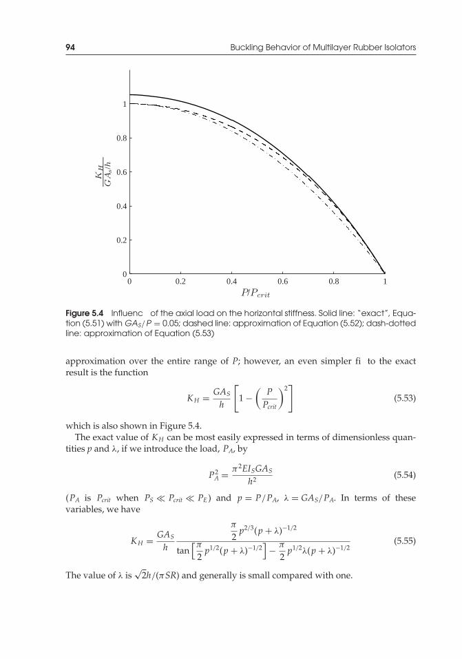
P1: TIX/XYZ P2: ABCJWST069-05 JWST069-Kelly-Style2 July 15, 2011 14:38 Printer Name: Yet to Come
94 Buckling Behavior of Multilayer Rubber Isolators
0 0.2 0.4 0.6 0.8 10
0.2
0.4
0.6
0.8
1K
H
GA
/h s
P/Pcrit
Figure 5.4 Influenc of the axial load on the horizontal stiffness. Solid line: “exact”, Equa-tion (5.51) with GAS/P = 0.05; dashed line: approximation of Equation (5.52); dash-dottedline: approximation of Equation (5.53)
approximation over the entire range of P; however, an even simpler fi to the exactresult is the function
KH = GAS
h
[1 −
(PPcrit
)2]
(5.53)
which is also shown in Figure 5.4.The exact value of KH can be most easily expressed in terms of dimensionless quan-
tities p and λ, if we introduce the load, PA, by
P2A = π2EISGAS
h2 (5.54)
(PA is Pcrit when PS Pcrit PE ) and p = P/PA, λ = GAS/PA. In terms of thesevariables, we have
KH = GAS
h
π
2p2/3(p + λ)−1/2
tan[π
2p1/2(p + λ)−1/2
]− π
2p1/2λ(p + λ)−1/2
(5.55)
The value of λ is√
2h/(πSR) and generally is small compared with one.
P1: TIX/XYZ P2: ABCJWST069-05 JWST069-Kelly-Style2 July 15, 2011 14:38 Printer Name: Yet to Come
Downward Displacement of the Top of a Bearing 95
5.4 Downward Displacement of the Top of a Bearing
The downward displacement of the top of a bearing due to a horizontal displacementis often needed in the design process, and this can also be calculated using the bucklinganalysis. Suppose that the bearing is just at critical load, but undeflected and imaginethe work done externally and internally as it moves to a buckled position. The externalwork is denoted by Pδv, where δv is the downward displacement, since we assume thatthe load remains constant during this process. The internal work, WD, is given by
WD = 12
h∫0
[V(v′ − ψ) + Mψ ′]dx (5.56)
but by equilibrium Equations (5.2a) and (5.2b),
V = −H0 + Pψ
M = M0 + H0x − Pv + Pv0
(5.57)
so that
WD = 12
h∫0
[(−H0 + Pψ) (v′ − ψ) + (M0 + H0x − Pv + Pv0) ψ ′] dx
= 12P
h∫0
(ψv′ − ψ2 − vψ ′) dx
−12H0
h∫0
[(v′ − ψ) − xψ ′]dx + (M0 + Pv0) [ψ(h) − ψ(0)] (5.58)
In the buckling problem, we have v0 = 0, ψ(0) = 0, ψ(h) = 0, and H0 = 0. Accordingly,the work equality becomes
Pδv = P2
h∫0
(2ψv′ − ψ2) dx (5.59)
The implication of this result is that the downward displacement is given by
δv = 12
h∫0
(2ψv′ − ψ2) dx (5.60)
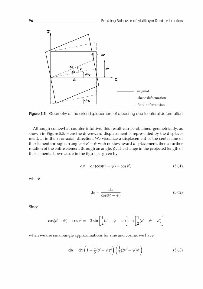
P1: TIX/XYZ P2: ABCJWST069-05 JWST069-Kelly-Style2 July 15, 2011 14:38 Printer Name: Yet to Come
96 Buckling Behavior of Multilayer Rubber Isolators
Figure 5.5 Geometry of the axial displacement of a bearing due to lateral deformation
Although somewhat counter intuitive, this result can be obtained geometrically, asshown in Figure 5.5. Here the downward displacement is represented by the displace-ment, u, in the x, or axial, direction. We visualize a displacement of the center line ofthe element through an angle of v′ − ψ with no downward displacement, then a furtherrotation of the entire element through an angle, ψ . The change in the projected length ofthe element, shown as du in the figu e, is given by
du = da (cos(v′ − ψ) − cos v′) (5.61)
where
da = dxcos(v′ − ψ)
(5.62)
Since
cos(v′ − ψ) − cos v′ = −2 sin[
12
(v′ − ψ + v′)]
sin[
12
(v′ − ψ − v′)]
when we use small-angle approximations for sine and cosine, we have
du = dx(
1 + 12
(v′ − ψ)2) (
12
(2v′ − ψ)ψ)
(5.63)
P1: TIX/XYZ P2: ABCJWST069-05 JWST069-Kelly-Style2 July 15, 2011 14:38 Printer Name: Yet to Come
Downward Displacement of the Top of a Bearing 97
leading to
δv = 12
h∫0
(2v′ − ψ)ψ dx (5.64)
When the bearing is buckled, the relationship between the vertical movement and thelateral displacement is given by Equation (5.64) by inserting
v(x) = δ
2
(1 − cos
πxh
)
ψ(x) = αβδ
2sin
πxh
(5.65)
giving
δv = 12
h∫0
(2αβδ
2π
hδ
2− α2β2δ2
4
)sin2 πx
hdx
= αβπ
8
(1 − αβh
2π
)δ2 (5.66)
At buckling, αh = π , so
δv = π2
8 hβ
(1 − β
2
)δ2 (5.67)
Since
β = GAS
GAS + Pcrit≈ GAS
Pcrit 1 (5.68)
δv = π 2GAS
8 hPcritδ2 (5.69)
Using the approximation for Pcrit in Equation (5.26) for a circular bearing with radiusR, we have
δv =√
2π
8SRδ2 (5.70)
which surprisingly does not depend on the height of the bearing. For example, supposeR = h, δ = h, S = 10, then
δv =√
2π
80h = 0.055 h
P1: TIX/XYZ P2: ABCJWST069-05 JWST069-Kelly-Style2 July 15, 2011 14:38 Printer Name: Yet to Come
98 Buckling Behavior of Multilayer Rubber Isolators
Although the same procedure can be used to estimate δv when P < Pcrit and the bearingis laterally displaced, the algebraic complexity has reached the point of diminishingreturns. A simpler model will be developed in Section 5.5.
The previous result Equation (5.60) can be used to calculate the displacement of thetop of the bearing when it is loaded by a lateral load FH and a downward vertical load P.
The starting point for the calculation is the solution for v(x) and ψ(x), namely
v(x) = FHαβP
[sin(αx) − αβx + 1 − cos(αh)
sin(αh)(1 − cos(αx))
](5.71)
and
ψ(x) = FHP
[1 − cos(αh)
sin(αh)sin(αx) − (1 − cos(αx))
](5.72)
from these, we have
v(h) = δh = FHαβP
(2
1 − cos(αh)sin(αh)
− αβh)
(5.73)
and
v′(x) = FHβP
(cos(αx) + 1 − cos(αh)
sin(αh)sin(αx) − β
)(5.74)
Using Equations (5.72) and (5.74), we form the product
2ψv′ − ψ2 = F 2H
βP2 {−2[β cos αh cos2 αx − β cos αh + cos αh − 2 cos αh cos2 αx
+ cos αh cos αx − 1 + sin αh sin αx − 2 sin αh cos αx sin αx
+β cos αx sin αx sin αh + cos αx]/[cos αh + 1]} (5.75)
Integrating this expression from x = 0 to x = h, and plugging into Equation (5.64)leads to
δv = 12F 2H
βP2
αhβ cos αh − 2 sin αh + 2αh − β sin αhα(cos αh + 1)
(5.76)
The terms FH and P can be eliminated by dividing this by the square of δh fromEquation (5.73), giving
δv =[αhβ
2αhβ cos(αh) − 2 sin(αh) + 2αh − β sin(αh)
−4 cos(αh) + β2α2h2 cos(αh) + 4 + β2α2h2 − 4βαh sin(αh)
]δ2h
h(5.77)
In Equation (5.77) the expression in the brackets is a function of the two dimensionlessquantities αh and β both of which depend on the vertical load P. The result shows
P1: TIX/XYZ P2: ABCJWST069-05 JWST069-Kelly-Style2 July 15, 2011 14:38 Printer Name: Yet to Come
Downward Displacement of the Top of a Bearing 99
that when the bearing parameters PS and PE are specified the vertical displacement isquadratic in the lateral displacement δh and can easily be computed for any value ofaxial load.
If we use the approximations made in the earlier section neglecting GAS as comparedwith P, giving αh = πp and β ≈ 0, this reduces to
δv = πGAS
4Pcrit
(πp − sin(πp)1 − cos(πp)
)δ2h
h= πGAS
4Pcritf (πp)
δ2h
h(5.78)
The function f (x) = (x − sin x)/(1 − cos x) varies from 0 when x = 0 to π/2 whenx = π and increases monotonically over the range 0 ≤ x ≤ π . When x is replaced by −x,it is anti-symmetric, i.e., f (−x) = − f (x). The derivative
f ′(x) = (1 − cos x) − x sin x(1 − cos x)2 (5.79)
is symmetric and varies from 1/3 to 1 as x varies from 0 to π and monotonically increasesover this range.
The vertical stiffness of the isolator in the undeformed position is given by
K 0v = Ec AS
h(5.80)
where Ec is the compression modulus given by
Ec = 6GS2 (5.81)
The vertical stiffness when sheared through a displacement δh will be
Kv =(
dδtv
dP
)−1
(5.82)
where
δtv = PhEc AS
+ δv (5.83)
Now
dδv
dP= dδv
dxdxdP
= π 2GAS
4P2crit
f ′(πp)δ2h
h(5.84)
giving
Kv = K 0v
1
1 + π2
4GASEc AS
P2crit
f ′(πp)δ2h
h
(5.85)
P1: TIX/XYZ P2: ABCJWST069-05 JWST069-Kelly-Style2 July 15, 2011 14:38 Printer Name: Yet to Come
100 Buckling Behavior of Multilayer Rubber Isolators
Since P2crit = GASEIS(π2/h2), this becomes
Kv = K 0v
1
1 + 34f ′(πp)
δ2h
r2
(5.86)
where r2 = I/A. For a circular bearing of diameter �, r 2 = �2/16 leading to
Kv = K 0v
1
1 + 12 f ′(πp)δ2h
�2
(5.87)
In many cases the displacement can be a significan fraction of the diameter so thatthe vertical stiffness can be considerably reduced by the lateral displacement. Thisresult has implications for the computer modelling of isolation bearings. The modelsof isolators in most structural analysis programs have two sets of independent springsthat represent the horizontal stiffness and the vertical stiffness. This result shows thatif we are to properly model an isolator, we need to include the interaction between thevertical stiffness and the horizontal displacement. In principle this could be done by afinit element model, but this is much too complicated to be included in a structuralanalysis program. In the next section, however, we will demonstrate a simple two-spring mechanical model that will very accurately represent the behavior of a bearingincluding interaction between these quantities, and that could be easily incorporatedinto a structural analysis program.
5.5 A Simple Mechanical Model for Bearing Buckling
There are a number of other aspects of bearing behavior that can be modelled using theshear-weak column theory, but the algebraic complexity becomes considerable and oneloses the direct physical understanding of the phenomenon that is useful in design. Theother aspects of bearing behavior that are useful to cover are the downward movement ofthe top of the bearing produced by horizontal displacement, the postbuckling behavior,and the influenc of the axial load on the damping in the bearing. To provide a simplephysical interpretation of these factors, a simple mechanical model with two mechanismsof deformation has been developed that closely fit the exact theory and demonstratesthese aspects of bearing behavior in a simple way.
In the model shown in Figure 5.6, two rigid elements in the shape of tees are connectedby moment springs across hinges at top and bottom and by shear springs and friction-less rollers at mid-height. The two deformation variables shown are shear displacement,s, and relative rotation, θ ; the two moment spring stiffnesses are shown as K1/2 each(moment/radian), the shear spring stiffness as K2 (shear force/displacement), the ver-tical load as P, and the horizontal load at the top of the column as FH . The horizontaldisplacement, v, of the top of the column is given, in terms of s and θ , by
v = h sin θ + s cos θ (5.88)
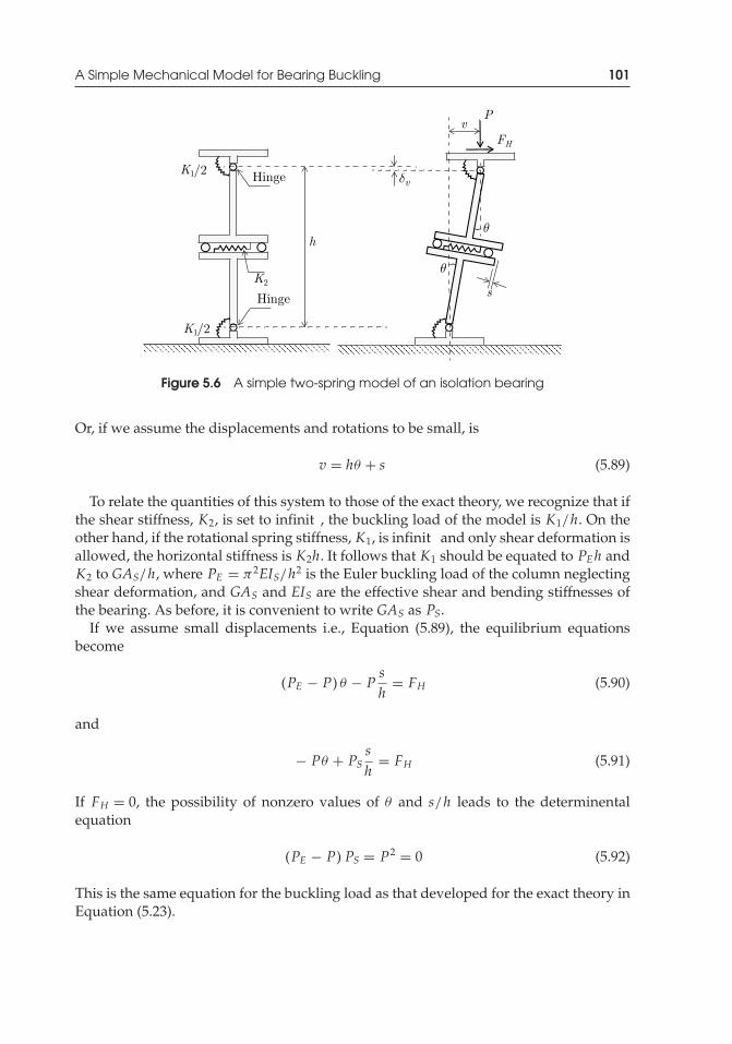
P1: TIX/XYZ P2: ABCJWST069-05 JWST069-Kelly-Style2 July 15, 2011 14:38 Printer Name: Yet to Come
A Simple Mechanical Model for Bearing Buckling 101
Figure 5.6 A simple two-spring model of an isolation bearing
Or, if we assume the displacements and rotations to be small, is
v = hθ + s (5.89)
To relate the quantities of this system to those of the exact theory, we recognize that ifthe shear stiffness, K2, is set to infinit , the buckling load of the model is K1/h. On theother hand, if the rotational spring stiffness, K1, is infinit and only shear deformation isallowed, the horizontal stiffness is K2h. It follows that K1 should be equated to PEh andK2 to GAS/h, where PE = π2EIS/h2 is the Euler buckling load of the column neglectingshear deformation, and GAS and EIS are the effective shear and bending stiffnesses ofthe bearing. As before, it is convenient to write GAS as PS.
If we assume small displacements i.e., Equation (5.89), the equilibrium equationsbecome
(PE − P) θ − Psh
= FH (5.90)
and
− Pθ + PSsh
= FH (5.91)
If FH = 0, the possibility of nonzero values of θ and s/h leads to the determinentalequation
(PE − P) PS = P2 = 0 (5.92)
This is the same equation for the buckling load as that developed for the exact theory inEquation (5.23).

P1: TIX/XYZ P2: ABCJWST069-05 JWST069-Kelly-Style2 July 15, 2011 14:38 Printer Name: Yet to Come
102 Buckling Behavior of Multilayer Rubber Isolators
When the horizontal force, FH , is present, the solutions for θ and s are
θ = FHPS + P
PSPE − PPS − P2
sh = FH
PEPSPE − PPS − P2
(5.93)
The horizontal stiffness of the model is given by
KH = FH/v (5.94)
and
v = hθ + s = hFH (PS + P + PE )PSPE − PPS − P2 (5.95)
so that
KH = 1hPSPE − PPS − P2
PE + P + PS(5.96)
To the same order of approximation that gave the buckling load as (PE PS)1/2, thisresult reduces to
KH = GAS
h
(1 − P2
PSPE
)(5.97)
This result is identical to the approximate Equation (5.53) and is plotted in Figure 5.4 forcomparison with the exact formula, Equation (5.51), for GAS/P = 0.05.
The downward movement of the top of the bearing due to the horizontal displacementcan also be derived from this model. The height reduction of a bearing is often useful toknow for detailing adjacent foundation components. If we assume a small rotation, thedownward movement of the top of the bearing, denoted by δv, is given by
δv = sθ + hθ2/2 (5.98)
If we substitute for θ and s/h, using Equation (5.93), and eliminate FH in terms of v fromEquation (5.95), we have
δv = v2
2 h(GAS + P) (GAS + P + 2PE )
(GAS + P + PE )2 (5.99)
Since PE is very much larger than P or PS, we can approximate this expression by
δv = v2
hGAS + P
PE(5.100)
P1: TIX/XYZ P2: ABCJWST069-05 JWST069-Kelly-Style2 July 15, 2011 14:38 Printer Name: Yet to Come
A Simple Mechanical Model for Bearing Buckling 103
Koh and Kelly (1987) presented the exact form of this result. The result above, however,is considerably simpler and has been verifie by experimental work presented in thesame publication. This simplifie result is very useful for practical applications andcan be used to estimate the vertical stiffness of an isolator in a deformed position. Thisparameter is necessary for some applications, and the standard recommendation is touse the formula KV = Ec A/tr , replacing the area, A, by the area of overlap betweenthe top plate and the bottom plate when the bearing is displaced horizontally. Thisvery simplistic approach is not based on rational analysis; it ignores the fact that thedownward movement of the top of the bearing (with respect to the bottom duringlateral displacement) is caused by a tilting of the reinforcing layers at the middle of thebearing away from the end restraints. This tilting process means that some of the layersexperience a shear stress produced by the component of the vertical load in the directionof the rotated plates.
Thus, if we take the horizontal displacement, v, to be f xed and vary load P, theadditional displacement, δv, due to the column action of the bearing is given byEquation (5.100), and the total vertical displacement, which includes δv and the com-pression of the rubber, δtv, is
δtv = PhEc AS
+ GAS + PPE
v2
h(5.101)
The instantaneous vertical stiffness is given by
KV = dPdδ
tv
= 1h/ (Ec AS) + v2/ (PEh)
(5.102)
Recalling that PE = π2EIS/(3 h2), this reduces to
KV = Ec ASh
11 + (3v2) / (π2r2)
(5.103)
For a circular bearing, r = �/4; therefore
3v2
πr2 = 1 (5.104)
when
v2 = π2
3�2
16(5.105)
or when
v = 1√3
π
4� = 0.45 � (5.106)

P1: TIX/XYZ P2: ABCJWST069-05 JWST069-Kelly-Style2 July 15, 2011 14:38 Printer Name: Yet to Come
104 Buckling Behavior of Multilayer Rubber Isolators
It follows that the influenc of horizontal displacement on the vertical stiffness can playa significan role at displacements that are comparable to the bearing diameter.
5.5.1 Postbuckling Behavior
The behavior of a bearing under large displacements can be described by the simpletwo-spring model if we do not linearize the equations of equilibrium, but retain theexact trigonometric terms. The equations of equilibrium are
Pv + hFH cos θ = PEh θ
P sin θ + FH cos θ = PSsh
(5.107)
(where the small term FHs sin θ has been neglected) with displacement v related to θ
and h by Equation (5.88). The second of the equations of equilibrium allows us to solvefor s/h in terms of θ , which when substituted into the firs equation gives
P sin θ + P (FH cos θ + P sin θ)PS
cos θ + FH cos θ = PEθ (5.108)
Equations (5.88) and (5.108) can be used in two ways. We can fi FH and solve the secondas a quadratic equation for P in terms of θ , and from the first we can determine the valueof v that corresponds to this value of P, thus obtaining a relationship for P as a functionof horizontal displacement v. For example, to determine whether or not the postbuckledstate is stable, we set FH = 0 and solve for P to obtain
P = PS2 cos θ
[(1 + 4
PEPS
θ
tan θ
)1/2
− 1
](5.109)
and
vh
= sin θ
2
[1 +
(1 + 4
PEPS
θ
tan θ
)1/2]
(5.110)
The dominant term in both equations is PE/PS, and to the same level of approximationthat gave the critical load as (PS/PE )1/2, these two equations can be approximated by
P = (PSPE )1/2
cos θ
(θ
tan θ
)1/2
(5.111)
and
vh
= sin θ
(PEPS
)1/2 (θ
tan θ
)1/2
(5.112)
P1: TIX/XYZ P2: ABCJWST069-05 JWST069-Kelly-Style2 July 15, 2011 14:38 Printer Name: Yet to Come
A Simple Mechanical Model for Bearing Buckling 105
To determine whether the bearing is stable in the postbuckled configuration it is onlynecessary to determine the sign of dP/dv. Now
dPdv
= dPd θ
d θ
dv(5.113)
and
dPd θ
= (PE PS)1/2(
sin(2 θ )2 θ
)1/2 sin(2 θ ) − 2 θ cos(2θ )(sin(2 θ ))2
dvd θ
= h (PE PS)1/2(
2θ sin(2 θ )
)1/2 sin(2 θ ) − 2 θ cos(2 θ )4
(5.114)
so that
dPdv
= PSh
sin(2 θ ) − 2 θ cos(2 θ )sin(2 θ )(sin(2 θ ) + 2 θ cos(2 θ ))
(5.115)
which can be written as
dPdv
= PSh
tan(2 θ ) − 2 θ
sin(2 θ )(tan(2 θ ) + 2 θ )(5.116)
Now, tan(2θ ) > 2θ for 0 < θ < π/2, so that dP/dv > 0 over this range, therefore, thebearing is stable (i.e., the equilibrium load P increases as v increases).
Another way to interpret the equations is to assume that P is fixed solve the firsequation for FH as a function of θ , the second equation for v as a function of θ , and thendetermine a relationship for FH as a function of v for constant P. First we get
FH = PSPE θ − PPS sin θ − P2 sin θ cos θ
cos θ (PS + P cos θ )(5.117)
and the second equation
vh
= sin θ
(PPS
cos θ + 1)
+ FH cos2 θ
PS(5.118)
becomes
vh
= PE θ cos θ + P cos θ sin θ + PS sin θ
PS + P cos θ(5.119)
By making the same approximations as before, these become
FH = PE PS θ − P2 sin θ cos θ
P cos2 θ(5.120)
P1: TIX/XYZ P2: ABCJWST069-05 JWST069-Kelly-Style2 July 15, 2011 14:38 Printer Name: Yet to Come
106 Buckling Behavior of Multilayer Rubber Isolators
and
vh
= PE θ + P sin θ
P(5.121)
Again, we are interested in the sign of the derivative dFH/dv, for if it becomes negative,it implies that the bearing could become unstable under a lateral force, FH , for verticalloads that do not exceed (PSPE )1/2. Proceeding in the same way as before, we have
dFHd θ
= PSPE (cos θ + 2 θ sin θ ) − P2(cos θ cos(2θ ) + sin θ sin(2θ ))P cos3 θ
(5.122)
and
dvdθ
= hPE + P cos θ
P(5.123)
so that
dFHdv
= PhPSPE (cos θ + 2θ sin θ ) − P2 cos θ
(PE + P cos θ ) cos3 θ(5.124)
The denominator of this expression is always positive, and the numerator is positive if
PSPEP2 >
cos θ
cos θ + 2θ sin θ= 1
1 + 2θ tan θ(5.125)
Now, PSPE/P2 will always be greater than 1, and because θ tan θ > 0 for 0 < θ < π/2,the right-hand side is always less than one over this range, therefore, the bearing isalways stable.
5.5.2 Influenc of Compressive Load on Bearing Damping Properties
The simple two-spring model can also be used to estimate the effect of the verticalload on the damping properties of a bearing. In this case we replace E and G byE∗ = E(1 + i tan δ) and G by G∗ = G(1 + i tan δ), where δ is define as the loss angleof the material and tan δ the loss factor of the rubber. The corresponding quantities, P∗
E ,P∗S , are define as
P∗E = PE (1 + i tan δ)
P∗S = PS(1 + i tan δ)
(5.126)
The horizontal stiffness becomes
K ∗H = P∗
S
hP∗S P
∗E − PP∗
S − P2
P∗S P
∗E + PP∗
S + P∗2S
(5.127)
P1: TIX/XYZ P2: ABCJWST069-05 JWST069-Kelly-Style2 July 15, 2011 14:38 Printer Name: Yet to Come
A Simple Mechanical Model for Bearing Buckling 107
The corresponding complex rotations, θ∗, and shear deformation, s∗, are given by
θ∗ = FHP∗S + P
P∗S P
∗E − PP∗
S − P2
s∗
h= FH
P∗E
P∗S P
∗E − PP∗
S − P2
(5.128)
from which we see that the phase angle for θ∗ and s∗ differs if δ �= 0.The dynamic shear stiffness of the bearing, KD, is define by
KD = ∣∣K ∗H
∣∣ (5.129)
and the loss factor, tan η, for the bearing, as opposed to that for the material (e.g., tan δ), isdefine by
tan η = Im(K ∗H)
Re(K ∗H
) (5.130)
The results for a number of cases can be evaluated easily. For example, if PE � GAS > P ,which define the case when the entire deformation is shear deformation, the loss factorfor the bearing becomes
tan η = tan δ (5.131)
Thus, the loss factor is unaffected by compressive load, and no amplificatio of thedamping occurs. On the other hand, if PS = GAS � PE > P , which is the situation thatleads to flexura deformation only, the loss factor of the bearing becomes
tan η = tan δ
1 − P/PE(5.132)
In this case the buckling load is PE ; therefore, although an amplificatio of the dampingoccurs, it is solely due to the reduction in the stiffness, i.e., Re(K ∗
H), as a result of the axialload. There is no increase in the energy dissipated over a complete cycle.
For the typical bearing where PE � GAS but P > GAS, the result for the lossfactor becomes
tan η = tan δ1 + tan2 δ + P2/P2
crit
1 + tan2 δ − P2/P2crit
(5.133)
where Pcrit = √PE PS. The term in the denominator comes from the reduction in the
stiffness, but the term in the numerator shows that the total energy dissipated in a cycleincreases. This increase in the energy dissipation in a cycle is due to the compressionload increasing the phase difference between the force, FH , and displacement, v, throughits effects on θ and s. It is also significan that the dynamic stiffness, KD, does not vanish
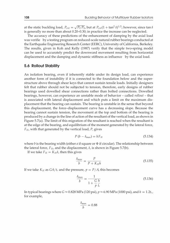
P1: TIX/XYZ P2: ABCJWST069-05 JWST069-Kelly-Style2 July 15, 2011 14:38 Printer Name: Yet to Come
108 Buckling Behavior of Multilayer Rubber Isolators
at the static buckling load, Pcrit = √PE PS, but at Pcrit(1 + tan2 δ)1/2; however, since tan δ
is generally no more than about 0.20–0.30; in practice the increase can be neglected.The accuracy of these predictions of the enhancement of damping by the axial load
was verifie by a testing program on reduced-scale natural rubber bearings conducted atthe Earthquake Engineering Research Center (EERC), University of California, Berkeley.The results, given in Koh and Kelly (1987) verify that the simple two-spring modelcan be used to accurately predict the downward movement resulting from horizontaldisplacement and the damping and dynamic stiffness as influence by the axial load.
5.6 Rollout Stability
An isolation bearing, even if inherently stable under its design load, can experienceanother form of instability if it is connected to the foundation below and the super-structure above through shear keys that cannot sustain tensile loads. Initially designersfelt that rubber should not be subjected to tension, therefore, early designs of rubberbearings used dowelled shear connections rather than bolted connections. Dowelledbearings, however, can experience an unstable mode of behavior – called rollout – thatis associated with lateral displacement and which puts a limit on the maximum dis-placement that the bearing can sustain. The bearing is unstable in the sense that beyondthis displacement, the force–displacement curve has a decreasing slope. Because thebearing cannot sustain tension, the movement at the top and bottom of the bearing isproduced by a change in the line of action of the resultant of the vertical load, as shown inFigure 5.7(a). The limit of this migration of the resultant is reached when the resultant isat the edge of the bearing, and equilibrium of the moment generated by the lateral force,FH , with that generated by the vertical load, P, gives
P (b − δmax) = hFH (5.134)
where b is the bearing width (either a if square or � if circular). The relationship betweenthe lateral force, FH , and the displacement, δ, is shown in Figure 5.7(b).
If we take FH = KHδ, then this gives
δmax
b= P
P + KHh(5.135)
If we take KH as GA/tr and the pressure, p = P/A, this becomes
δmax
b= 1
1 + Gphtr
(5.136)
In typical bearings whereG≈ 0.828 MPa (120 psi), p≈ 6.90 MPa (1000 psi), and h = 1.2tr ,for example,
δmax
b= 0.88
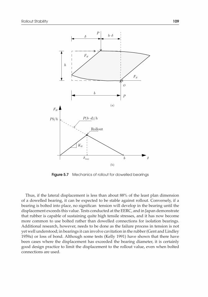
P1: TIX/XYZ P2: ABCJWST069-05 JWST069-Kelly-Style2 July 15, 2011 14:38 Printer Name: Yet to Come
Rollout Stability 109
Figure 5.7 Mechanics of rollout for dowelled bearings
Thus, if the lateral displacement is less than about 88% of the least plan dimensionof a dowelled bearing, it can be expected to be stable against rollout. Conversely, if abearing is bolted into place, no significan tension will develop in the bearing until thedisplacement exceeds this value. Tests conducted at the EERC, and in Japan demonstratethat rubber is capable of sustaining quite high tensile stresses, and it has now becomemore common to use bolted rather than dowelled connections for isolation bearings.Additional research, however, needs to be done as the failure process in tension is notyet well understood; in bearings it can involve cavitation in the rubber (Gent and Lindley1959a) or loss of bond. Although some tests (Kelly 1991) have shown that there havebeen cases where the displacement has exceeded the bearing diameter, it is certainlygood design practice to limit the displacement to the rollout value, even when boltedconnections are used.
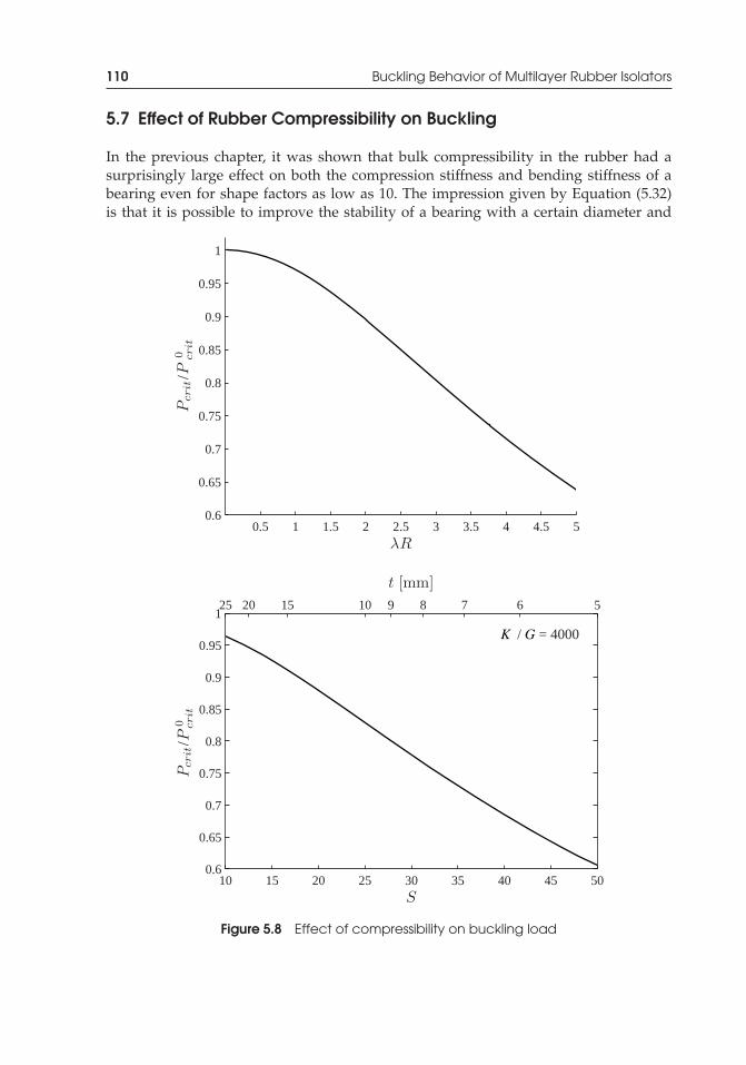
P1: TIX/XYZ P2: ABCJWST069-05 JWST069-Kelly-Style2 July 15, 2011 14:38 Printer Name: Yet to Come
110 Buckling Behavior of Multilayer Rubber Isolators
5.7 Effect of Rubber Compressibility on Buckling
In the previous chapter, it was shown that bulk compressibility in the rubber had asurprisingly large effect on both the compression stiffness and bending stiffness of abearing even for shape factors as low as 10. The impression given by Equation (5.32)is that it is possible to improve the stability of a bearing with a certain diameter and
0.5 1 1.5 2 2.5 3 3.5 4 4.5 50.6
0.65
0.7
0.75
0.8
0.85
0.9
0.95
1
Pcrit
/P0 crit
λR
10 15 20 25 30 35 40 45 500.6
0.65
0.7
0.75
0.8
0.85
0.9
0.95
1
Pcrit
/P0 crit
S
25 20 15 10 9 8 7 6 5
t [mm]
/ = 4000
Figure 5.8 Effect of compressibility on buckling load
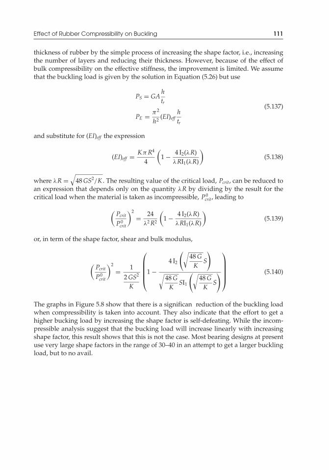
P1: TIX/XYZ P2: ABCJWST069-05 JWST069-Kelly-Style2 July 15, 2011 14:38 Printer Name: Yet to Come
Effect of Rubber Compressibility on Buckling 111
thickness of rubber by the simple process of increasing the shape factor, i.e., increasingthe number of layers and reducing their thickness. However, because of the effect ofbulk compressibility on the effective stiffness, the improvement is limited. We assumethat the buckling load is given by the solution in Equation (5.26) but use
PS = GAhtr
PE = π2
h2 (EI)effhtr
(5.137)
and substitute for (EI)eff the expression
(EI)eff = KπR4
4
(1 − 4 I2(λR)
λRI1(λR)
)(5.138)
where λR =√
48GS2/K . The resulting value of the critical load, Pcrit, can be reduced toan expression that depends only on the quantity λR by dividing by the result for thecritical load when the material is taken as incompressible, P0
crit, leading to
(PcritP0crit
)2
= 24λ2R2
(1 − 4 I2(λR)
λRI1(λR)
)(5.139)
or, in term of the shape factor, shear and bulk modulus,
(PcritP0crit
)2
= 1
2GS2
K
⎛⎜⎜⎜⎜⎝1 −
4 I2
(√48GK
S
)
√48GK
SI1
(√48GK
S
)
⎞⎟⎟⎟⎟⎠ (5.140)
The graphs in Figure 5.8 show that there is a significan reduction of the buckling loadwhen compressibility is taken into account. They also indicate that the effort to get ahigher bucking load by increasing the shape factor is self-defeating. While the incom-pressible analysis suggest that the bucking load will increase linearly with increasingshape factor, this result shows that this is not the case. Most bearing designs at presentuse very large shape factors in the range of 30–40 in an attempt to get a larger bucklingload, but to no avail.

P1: TIX/XYZ P2: ABCJWST069-05 JWST069-Kelly-Style2 July 15, 2011 14:38 Printer Name: Yet to Come
P1: TIX/XYZ P2: ABCJWST069-06 JWST069-Kelly-Style2 July 15, 2011 14:41 Printer Name: Yet to Come
6Buckling of MultilayerRubber Isolators in Tension
6.1 Introduction
We recall from the last chapter that the equation for the buckling of the isolator incompression is
P2 + PSP − PSPE = 0 (6.1)
where PS = GAS and PE = π2ESI/h2. This equation has two solutions, one of which ispositive and the other negative. These solutions are given by
Pcrit =−PS ±
√P2S + 4PSPE
2
The compression solution has been treated in detail in the last chapter. The negativesolution
Pcrit =−PS −
√P2S + 4PSPE
2(6.2)
implies that there exists a tensile buckling load, and the question now is the significancof that solution. The tensile critical load, which, if the isolator has a shape factor larger
The material in Sections 6.2 and 6.3 firs appeared in the article by Kelly, J. M. (2003). “TensionBuckling in Multilayer Elastomeric Bearings.” Journal of Engineering Mechanics (ASCE), 129(12), 1363–1368.DOI 10.1061/(ASCE)0733-9399(2003)129:12(1363). Reproduced with permission from ASCE.
Mechanics of Rubber Bearings for Seismic and Vibration Isolation, First Edition. James M. Kelly and Dimitrios A. Konstantinidis.C© 2011 John Wiley & Sons, Ltd. Published 2011 by John Wiley & Sons, Ltd.
113
P1: TIX/XYZ P2: ABCJWST069-06 JWST069-Kelly-Style2 July 15, 2011 14:41 Printer Name: Yet to Come
114 Buckling of Multilayer Rubber Isolators in Tension
than say 5, as shown in the previous chapter in Equation (5.26), is the negative of thecompression critical load. We can then defin a tension critical load by
Tcrit =√PSPE (6.3)
The unexpected implication of this result is that there is a tensile buckling load forthis type of rubber component that has the same numerical value as the compressionbuckling load. In addition, the quantities α and β when P is replaced by –T become
α2 = T(T − GAS)E ISGAS
(6.4)
β = − GAS
T − GAS(6.5)
so that if T > GAS, the buckled shape in tension is the same solution as in the com-pression case. Since the value of β is now negative, the rotation ψ(x) (Equation 5.20) isreversed, and the central layers are rotated in the direction that facilitates the upwardmovement of the top of the isolation through a shear deformation. Of course this buck-ling load could not be achieved in practice since the rubber will have cavitated beforethe bearing buckles, but the tensile buckling load and buckled shape are opposites ofthe compression case due to the fact that the deformation is entirely shear – and shear isintrinsically symmetric.
There are many examples of strange systems that buckle in tension, but these areentirely pathological in that the tension forces are always transferred to compressionelements that produce the instability. This is not the case here. The buckling processis really tensile. The linear elastic model that leads to both compression and tensionbuckling is an extremely simple one, and it might be argued that the tensile buck-ling may be an artifact of the model itself and not of the isolator. For this reason itwas decided to verify the results of the simple model by numerical simulation us-ing a finit element model of a multilayer rubber bearing to show that the predictionof tensile buckling by the simple linear elastic theory is in fact accurate and not anartifact of the way the model was set up. This numerical experiment, done in two di-mensions to reduce the size of the computation, simulates the behavior of a bearingin the shape of a long strip, and it shows clearly that tensile bucking is a real pos-sibility and not an artifact of the model. The essential point is that the mechanics ofthe isolator in tension are the mirror image of those of the isolator in compression.In particular when the isolator is in compression below the buckling load, but later-ally displaced, the layers in the center experience rotations that give the vertical loada component along the layer, causing a shear deformation. In tension the layers inthe center experience rotations in the opposite direction, giving a shear deformationdue to the tensile force that permits the top of the isolator to move upwards by amuch larger displacement than that which could be sustained in pure tension with nolateral displacement.
P1: TIX/XYZ P2: ABCJWST069-06 JWST069-Kelly-Style2 July 15, 2011 14:41 Printer Name: Yet to Come
Influenc of a Tensile Vertical Load on the Horizontal Stiffness 115
6.2 Influenc of a Tensile Vertical Load on the Horizontal Stiffness
If the load carried by a bearing is comparable to the buckling load, then the simpleformula for horizontal stiffness, KH = GA/tr = GAS/h, may need to be modified Theanalysis that led to the buckling load can be used to determine the effective horizontalstiffness in the presence of axial load. Consider a horizontal force, FH, at the top of abearing. When the resulting displacement at the top, v(h) = δh, is computed, then KH isgiven by
KH = FHv(h)
= FHδh
(6.6)
The basic equations, Equations (5.42a) and (5.42b), are solved using the boundaryconditions
v(0) = 0, ψ(0) = 0, ψ(h) = 0, H0 = −FH (6.7)
Thus
v(x) = A cos(αx) + B sin(αx) + M0
P− FH
Px (6.8a)
and
ψ(x) = αβ B cos (αx) − αβAsin (αx) − FHP
(6.8b)
Using the boundary conditions, we have
A= FHP
(cos(αh) − 1)1
αβ sin (αh)= −M0
P(6.9)
and
B = FHαβP
(6.10)
When these are substituted back into Equation (6.8a) we obtain
v(x) = FHαβP
[1 − cos(αh)
sin (αh)(1 − cos (αx)) + sin (αx) − αβx
](6.11a)
ψ(x) = FHP
[1 − cos (αh)
sin (αh)sin (αx) − (1 − cos (αx))
](6.11b)
P1: TIX/XYZ P2: ABCJWST069-06 JWST069-Kelly-Style2 July 15, 2011 14:41 Printer Name: Yet to Come
116 Buckling of Multilayer Rubber Isolators in Tension
The horizontal displacement at x = h is given by
δh = v(h) = FHαβP
(2 tan
(αh2
)− βαh
)(6.12)
and the rotation at x = h/2 is
ψ
(h2
)= FH
P
⎛⎜⎜⎝
1 − cos(
αh2
)
cos(
αh2
)⎞⎟⎟⎠ (6.13)
The horizontal stiffness KH is given by Equation (6.6)
KH = FHδh
= αβP
2 tan(
αh2
)− βαh
(6.14)
When P is replaced by –T, and T > GAS, both β and P change sign in Equation (6.14),and the stiffness is still positive, but the rotation at the center of the isolator changessign, facilitating the upward displacement of the top.
When T < GAS, the solution for this case will involve hyperbolic instead of trigono-metric functions, and, when T = GAS, the firs terms in the basic Equations (5.10a) and(5.10b) become indeterminate. The solutions for v(x) and ψ(x) for this case are
v(x) = FHGAS
x (6.15a)
ψ(x) = 0 (6.15b)
Thus the deformation is one of pure shear, and it is easy to show from Equation (5.60)that there is no change in height in the bearing (Kelly 2003).
The result for the influenc of the vertical load on the horizontal stiffness does notgive physical insight into the effect, but if we recall that the value of GAS is very small ascompared with PE and P, we can approximate αh and β by αh = πp (where p = P/Pcrit)and β ≈ GAS/P, which is much less than 1, giving
KH = GAS
hπp
2 tan(πp)(6.16)
which leads to KH = GAS/h = GA/tr as p → 0, and KH → 0 as p → 1. When P is replacedby –T and p by –t, where t = T/
√PE PS, we get the same result, showing that both P and
T affect the stiffness in a symmetric way.
P1: TIX/XYZ P2: ABCJWST069-06 JWST069-Kelly-Style2 July 15, 2011 14:41 Printer Name: Yet to Come
Vertical Displacement under Lateral Load 117
6.3 Vertical Displacement under Lateral Load
The previous result Equation (5.60) can be used to calculate the displacement of the topof the bearing when it is loaded by a lateral load FH and a tension load T > GAS.
The starting point for the calculation is the solution for v(x) and ψ(x), namely Equations(6.11a) and (6.11b). Evaluating Equation (6.11a) at x= hgives the horizontal displacement
δh = v(h) = FHαβP
(2
1 − cos (αh)sin (αh)
− βαh)
(6.17)
Differentiating (6.11a), we obtain
v′(x) = FHβP
(cos (αx) + 1 − cos (αh)
sin (αh)sin (αx) − β
)(6.18)
and using Equation (6.11b), we form the product
2ψv′ − ψ2 = F 2H
βP2 {−2[β cos αh cos2 αx − β cos αh + cos αh − 2 cos αh cos2 αx
+ cos αh cos αx − 1 + sin αh sin αx − 2 sin αh cos αx sin αx + β cos αx sin αx sin αh
+ cos αx]/[cos αh + 1]}
Integrating this expression from x = 0 to x = h gives
δv = 12
h∫0
(2ψv′ − ψ2) dx = 12F 2H
βP2
(αhβcos(αh) − 2sin(αh) + 2αh − β sin (αh)
α(cos(αh) + 1)
)(6.19)
The terms FH and P can be eliminated by dividing this by the square of δh from Equation(6.17), giving
δv = βαh2
(βαh cos (αh) − 2 sin(αh) + 2αh − β sin(αh)
−4 cos(αh) + β2α2h2 cos (αh) + 4 + β2α2h2 − 4βαh sin (αh)
)δ2h
h(6.20)
In Equation (6.20), the expression in the brackets is a function of the two dimensionlessquantities αh and β, both of which depend on the vertical load, P or T. The result showsthat when the bearing parameters PS and PE are specified the vertical displacement isquadratic in the lateral displacement δh and can easily be computed for any value ofaxial load, compressive or tensile.
If we use the approximations made in the earlier section neglecting GAS as comparedto P, giving αh = πp and β ≈ 0, this reduces to
δv = πGAS
4Pcrit
(πp − sin(πp)1 − cos(πp)
)δ2h
h= πGAS
4Pcritf (πp)
δ2h
h(6.21)
P1: TIX/XYZ P2: ABCJWST069-06 JWST069-Kelly-Style2 July 15, 2011 14:41 Printer Name: Yet to Come
118 Buckling of Multilayer Rubber Isolators in Tension
The function f (x) = (x − sin x)/(1 − cos x) varies from 0 when x = 0 to π/2 whenx = π and increases monotonically over the range 0 ≤ x ≤ π . When x is replacedby –x, it is antisymmetric, i.e., f (−x) = –f (x). The derivative
f ′(x) = 2(1 − cos x) − x sin x(1 − cos x)2 (6.22)
is symmetric and varies from 1/3 to 1 as x varies from 0 to π and monotonicallyincreases over this range, and at say x = π/2, which corresponds to p = 1/2, it has thevalue 0.429.
The vertical stiffness of the isolator in the undeformed position is given by
K 0v = Ec AS
h(6.23)
where Ec is the compression modulus. For a circular bearing, Ec = 6 GS2. The verticalstiffness when sheared through a displacement δh will be
Kv =(
dδtv
dP
)−1
(6.24)
where
δtv = PK 0v
+ δv = hEc AS
P + δv (6.25)
Now
dδv
dP= dδv
dxdxdP
= π 2
4GAS
P2crit
f ′(πp)δ2h
h(6.26)
giving
Kv = K 0v
1
1 + π2
4GASEc AS
P2crit
f ′(πp)δ2h
h2
(6.27)
Since P2crit = GASEIS(π2/h2), this becomes
Kv = K 0v
1
1 + 34f ′(πp)
δ2h
r2
(6.28)
P1: TIX/XYZ P2: ABCJWST069-06 JWST069-Kelly-Style2 July 15, 2011 14:41 Printer Name: Yet to Come
Vertical Displacement under Lateral Load 119
where r2 = I/A. For a circular bearing of diameter �, r2 = �2/16 leading to
Kv = K 0v
1
1 + 12 f ′(πp)δ2h
�2
(6.29)
In many cases, the displacement that is calculated from code requirements at extremeseismic loads can be a significan fraction of the diameter so that the vertical stiffness inboth compression and tension is considerably reduced by the lateral displacement. Forexample, if δh = 0.5� and p = P/Pcrit = 0.5, then Equation (6.29) gives Kv = 0.437K 0
v .While the bearings are normally in compression, the code requirements for base-isolatedtall buildings in near-fault locations can lead to situations where peripheral bearings inthe isolation system can be required to take some amount of tension. This tension iscaused by global overturning of the building produced by the lateral inertial force at thecenter of the mass of the building. The maximum inertial force and the resulting maxi-mum overturning moment occur at the same time as the maximum lateral displacementof the isolators, which at firs sight would seem to be a critical situation. It is well knownthat elastomers, such as natural rubber (polyisoprene) or neoprene (polycloroprene),will cavitate at a negative pressure of around 3G (Gent 1990). Since the value of G is inthe range 0.5 to 1.0 MPa (75 to 150 psi), and the state of internal stress in a thin layerof a multilayer isolator is virtually hydrostatic, the tension stress to produce cavitationis quite low. The tensile strain is also extremely small, since the stiffness of an isolatorin tension before cavitation occurs is the same as that in compression. The effectivecompression modulus Ec of a circular pad of rubber is 6 GS2, where S is the shape factorof an individual layer of the isolator, which can be in the range of 10 to 20, so that thetensile strain εt at the onset of cavitation will be εt = 1/(2S2), and the correspondingupward displacement will be of the order of a few millimeters or less.
So concerned are design engineers that an isolator not experience tension due to uplift,that many have resorted to a design approach called “loose bolts.” This certainly solvesthe tension problem, but raises other questions such as the reliability of the bolts if upliftshould occur, since the bolts will have to transfer the shear load to the isolator whileacting as cantilever elements. Other strategies have been tried, but each approach toeliminating tension has its own disadvantages.
All current seismic isolation codes require that the prototype tests include an uplifttest if uplift is predicted by analysis. In two seismic isolation projects, isolators weredisplaced laterally to very large displacements, and then the top of the isolator wasjacked up by, in one case, 12.5 mm (0.5 inch) and, in the other, by 19.0 mm (0.75 inch).In neither case did the test isolators fail, but clearly the tensile strain greatly exceeds thestrain at cavitation. The value of the buckling theory is to explain how the isolators cansurvive this tensile loading. The essential point is that the mechanics of the isolator intension are the mirror image of those for the isolator in compression. In particular whenthe isolator is in compression below the buckling load but laterally displaced, the layersin the center experience a rotation which gives the vertical load a component along thelayer and induces a shear deformation. In tension, the layers in the center experience a

P1: TIX/XYZ P2: ABCJWST069-06 JWST069-Kelly-Style2 July 15, 2011 14:41 Printer Name: Yet to Come
120 Buckling of Multilayer Rubber Isolators in Tension
rotation in the opposite direction, which allows a shear deformation caused by the tensileforce and permits the top of the isolator to move upwards by a much larger displacementthan that which could be sustained in pure tension with no lateral displacement. Thus thesimultaneous occurrence of tension and shear allows the isolator to avoid the damageof cavitation. The rubber can sustain only small strains in the state of triaxial stressgenerated by pure tension on a multilayer isolator with a large shape factor, but cansustain shear strains on the order of 500 or 600%. Thus the simultaneous occurrence oftension and shear allows the isolator to avoid the damaging effects of cavitation.
6.4 Numerical Modelling of Buckling in Tension
6.4.1 Modelling Details
In order to verify that the tension buckling predicted by the simple analytical theoryis real, the general purpose finit element ABAQUS (HKS 2001) was used to model asteel-reinforced multilayer bearing and to study its buckling behavior in both tensionand compression. The complete details of the procedure are given in (Kelly and Takhirov2004). Five finit element models of a bearing were created. These numerical models allhave the same width, the same total rubber thickness, and all the steel shims have thesame thickness. The only difference between the models is the shape factor of the rubberlayers. The total thickness of rubber is the same in each model, but the thickness ofthe rubber layer varies from model to model. The correspondence between the modelnumber and the layer thickness is given in Table 6.1.
The bearings are visualized as being long strip isolators, as shown in Figure 6.1, andthe finit element analysis is restricted to plane strain. Thus the numerical solutions tobe described in the next sections are based on a two-dimensional analysis of an isolatorwith infinit length.
The y-axis of the coordinate system is a vertical axis that extends across the steel shimsand rubber layers, and the horizontal axis x corresponds to the lateral direction of thebearing, as shown in Figure 6.1. Generally steel-reinforced rubber bearings have a holein the middle of the steel plates and a rubber cover on the traction-free sides of the
Table 6.1 Finite element models with various shape factors
Modelname
Steel shimthickness
[mm]
Total rubberthickness
[mm]Width[mm]
Rubber layerthickness
[mm]Shapefactor
Model 1 2.60 80.01 160.02 5.72 14Model 2 2.60 80.01 160.02 8.00 10Model 3 2.60 80.01 160.02 11.43 7Model 4 2.60 80.01 160.02 16.00 5Model 5 2.60 80.01 160.02 26.67 3
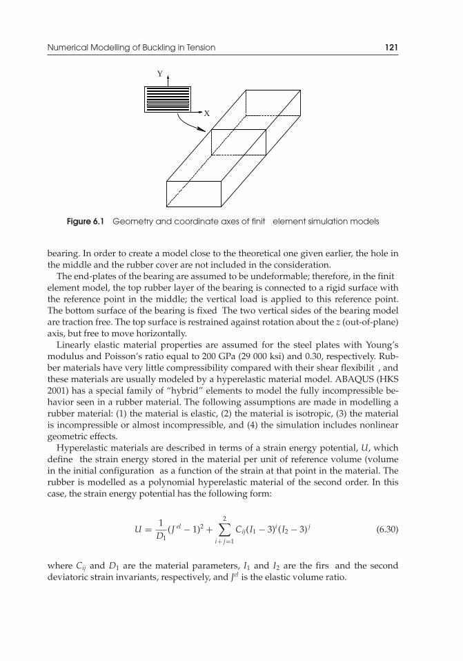
P1: TIX/XYZ P2: ABCJWST069-06 JWST069-Kelly-Style2 July 15, 2011 14:41 Printer Name: Yet to Come
Numerical Modelling of Buckling in Tension 121
Y
X
Figure 6.1 Geometry and coordinate axes of finit element simulation models
bearing. In order to create a model close to the theoretical one given earlier, the hole inthe middle and the rubber cover are not included in the consideration.
The end-plates of the bearing are assumed to be undeformable; therefore, in the finitelement model, the top rubber layer of the bearing is connected to a rigid surface withthe reference point in the middle; the vertical load is applied to this reference point.The bottom surface of the bearing is fixed The two vertical sides of the bearing modelare traction free. The top surface is restrained against rotation about the z (out-of-plane)axis, but free to move horizontally.
Linearly elastic material properties are assumed for the steel plates with Young’smodulus and Poisson’s ratio equal to 200 GPa (29 000 ksi) and 0.30, respectively. Rub-ber materials have very little compressibility compared with their shear flexibilit , andthese materials are usually modeled by a hyperelastic material model. ABAQUS (HKS2001) has a special family of “hybrid” elements to model the fully incompressible be-havior seen in a rubber material. The following assumptions are made in modelling arubber material: (1) the material is elastic, (2) the material is isotropic, (3) the materialis incompressible or almost incompressible, and (4) the simulation includes nonlineargeometric effects.
Hyperelastic materials are described in terms of a strain energy potential, U, whichdefine the strain energy stored in the material per unit of reference volume (volumein the initial configuration as a function of the strain at that point in the material. Therubber is modelled as a polynomial hyperelastic material of the second order. In thiscase, the strain energy potential has the following form:
U = 1D1
(J el − 1)2 +2∑
i+ j=1
Cij(I1 − 3)i (I2 − 3) j (6.30)
where Cij and D1 are the material parameters, I1 and I2 are the firs and the seconddeviatoric strain invariants, respectively, and Jel is the elastic volume ratio.
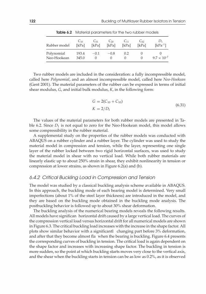
P1: TIX/XYZ P2: ABCJWST069-06 JWST069-Kelly-Style2 July 15, 2011 14:41 Printer Name: Yet to Come
122 Buckling of Multilayer Rubber Isolators in Tension
Table 6.2 Material parameters for the two rubber models
C10 C01 C20 C11 C02 D1
Rubber model [kPa] [kPa] [kPa] [kPa] [kPa] [kPa–1]
Polynomial 193.4 −0.1 −0.8 0.2 0 0Neo-Hookean 345.0 0 0 0 0 9.7 × 10⁻⁷
Two rubber models are included in the consideration: a fully incompressible model,called here Polynomial, and an almost incompressible model, called here Neo-Hookean(Gent 2001). The material parameters of the rubber can be expressed in terms of initialshear modulus, G, and initial bulk modulus, K, in the following form:
G = 2(C10 + C10)
K = 2/D1(6.31)
The values of the material parameters for both rubber models are presented in Ta-ble 6.2. Since D1 is not equal to zero for the Neo-Hookean model, this model allowssome compressibility in the rubber material.
A supplemental study on the properties of the rubber models was conducted withABAQUS on a rubber cylinder and a rubber layer. The cylinder was used to study thematerial model in compression and tension, while the layer, representing one singlelayer of the rubber locked between two rigid horizontal surfaces, was used to studythe material model in shear with no vertical load. While both rubber materials arelinearly elastic up to about 250% strain in shear, they exhibit nonlinearity in tension orcompression at lower strains, as shown in Figure 6.2(a) and (b).
6.4.2 Critical Buckling Load in Compression and Tension
The model was studied by a classical buckling analysis scheme available in ABAQUS.In this approach, the buckling mode of each bearing model is determined. Very smallimperfections (about 1% of the steel layer thickness) are introduced in the model, andthey are based on the buckling mode obtained in the buckling mode analysis. Thepostbuckling behavior is followed up to about 30% shear deformation.
The buckling analysis of the numerical bearing models reveals the following results.All models have significan horizontal drift caused by a large vertical load. The curves ofthe compression vertical load versus horizontal drift for all numerical models are shownin Figure 6.3. The critical buckling load increases with the increase in the shape factor. Allplots show similar behavior with a significantl changing part before 3% deformation,and after that they become almost fla when the bearing is buckling. Figure 6.4 presentsthe corresponding curves of buckling in tension. The critical load is again dependent onthe shape factor and increases with increasing shape factor. The buckling in tension ismore sudden, so the point at which buckling starts moves very close to the vertical axis,and the shear when the buckling starts in tension can be as low as 0.2%, as it is observed
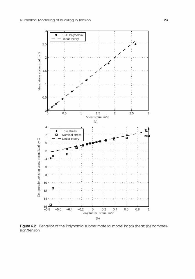
P1: TIX/XYZ P2: ABCJWST069-06 JWST069-Kelly-Style2 July 15, 2011 14:41 Printer Name: Yet to Come
Numerical Modelling of Buckling in Tension 123
0 0.5 1 1.5 2 2.5 30
0.5
1
1.5
2
2.5
3
Shear strain, in/in
She
ar s
tres
s no
rmal
ized
by
GFEA: PolynomialLinear theory
8 6 4 2 0 0.2 0.4 0.6 0.8 1
0
2
4
Longitudinal strain, in/in
Com
pres
sion
/ten
sion
str
ess
norm
aliz
ed b
y G
True stressNominal stressLinear theory
(a)
(b)
Figure 6.2 Behavior of the Polynomial rubber material model in: (a) shear; (b) compres-sion/tension
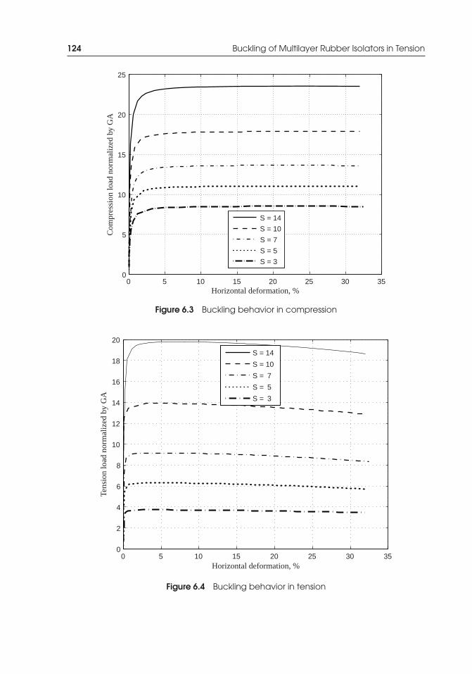
P1: TIX/XYZ P2: ABCJWST069-06 JWST069-Kelly-Style2 July 15, 2011 14:41 Printer Name: Yet to Come
124 Buckling of Multilayer Rubber Isolators in Tension
0 5 10 15 20 25 30 350
5
10
15
20
25
Horizontal deformation, %
Com
pres
sion
load
nor
mal
ized
by
GA
S = 14
S = 10
S = 7
S = 5
S = 3
Figure 6.3 Buckling behavior in compression
0 5 10 15 20 25 30 350
2
4
6
8
10
12
14
16
18
20
Horizontal deformation, %
Tens
ion
load
nor
mal
ized
by
GA
S = 14
S = 10
S = 7
S = 5
S = 3
Figure 6.4 Buckling behavior in tension
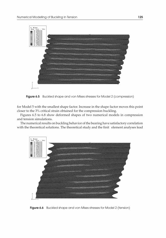
P1: TIX/XYZ P2: ABCJWST069-06 JWST069-Kelly-Style2 July 15, 2011 14:41 Printer Name: Yet to Come
Numerical Modelling of Buckling in Tension 125
(Ave. Crit.: 75%)S, Mises
+2.670e+00+1.744e+03+3.485e+03+5.226e+03+6.967e+03+8.708e+03+1.045e+04+1.219e+04+1.393e+04+1.567e+04+1.741e+04+1.915e+04+2.089e+04
1
2
3
Figure 6.5 Buckled shape and von Mises stresses for Model 2 (compression)
for Model 5 with the smallest shape factor. Increase in the shape factor moves this pointcloser to the 3% critical strain obtained for the compression buckling.
Figures 6.5 to 6.8 show deformed shapes of two numerical models in compressionand tension simulations.
The numerical results on buckling behavior of the bearing have satisfactory correlationwith the theoretical solutions. The theoretical study and the finit element analyses lead
(Ave. Crit.: 75%)S, Mises
+2.701e+00+2.737e+03+5.471e+03+8.205e+03+1.094e+04+1.367e+04+1.641e+04+1.914e+04+2.188e+04+2.461e+04+2.734e+04+3.008e+04+3.281e+04
1
2
3
Figure 6.6 Buckled shape and von Mises stresses for Model 2 (tension)
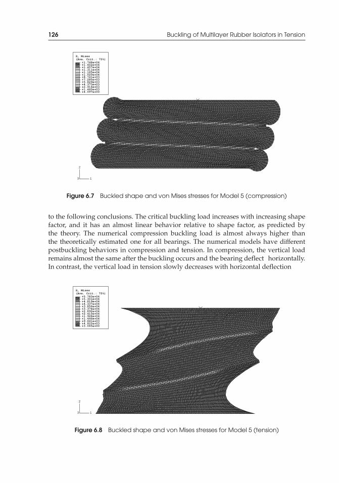
P1: TIX/XYZ P2: ABCJWST069-06 JWST069-Kelly-Style2 July 15, 2011 14:41 Printer Name: Yet to Come
126 Buckling of Multilayer Rubber Isolators in Tension
(Ave. Crit.: 75%)S, Mises
+4.097e+00+1.460e+03+2.916e+03+4.373e+03+5.829e+03+7.285e+03+8.741e+03+1.020e+04+1.165e+04+1.311e+04+1.457e+04+1.602e+04+1.748e+04
1
2
3
Figure 6.7 Buckled shape and von Mises stresses for Model 5 (compression)
to the following conclusions. The critical buckling load increases with increasing shapefactor, and it has an almost linear behavior relative to shape factor, as predicted bythe theory. The numerical compression buckling load is almost always higher thanthe theoretically estimated one for all bearings. The numerical models have differentpostbuckling behaviors in compression and tension. In compression, the vertical loadremains almost the same after the buckling occurs and the bearing deflect horizontally.In contrast, the vertical load in tension slowly decreases with horizontal deflection
(Ave. Crit.: 75%)S, Mises
+3.065e+00+4.822e+03+9.641e+03+1.446e+04+1.928e+04+2.410e+04+2.892e+04+3.374e+04+3.856e+04+4.337e+04+4.819e+04+5.301e+04+5.783e+04
1
2
3
Figure 6.8 Buckled shape and von Mises stresses for Model 5 (tension)
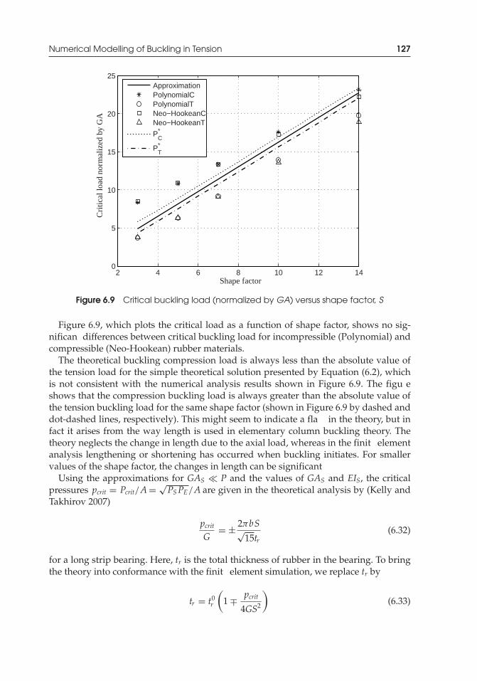
P1: TIX/XYZ P2: ABCJWST069-06 JWST069-Kelly-Style2 July 15, 2011 14:41 Printer Name: Yet to Come
Numerical Modelling of Buckling in Tension 127
2 4 6 8 10 12 140
5
10
15
20
25
Shape factor
Cri
tica
l loa
d no
rmal
ized
by
GA
ApproximationPolynomialCPolynomialTNeo−HookeanCNeo−HookeanT
PC*
PT*
Figure 6.9 Critical buckling load (normalized by GA) versus shape factor, S
Figure 6.9, which plots the critical load as a function of shape factor, shows no sig-nifican differences between critical buckling load for incompressible (Polynomial) andcompressible (Neo-Hookean) rubber materials.
The theoretical buckling compression load is always less than the absolute value ofthe tension load for the simple theoretical solution presented by Equation (6.2), whichis not consistent with the numerical analysis results shown in Figure 6.9. The figu eshows that the compression buckling load is always greater than the absolute value ofthe tension buckling load for the same shape factor (shown in Figure 6.9 by dashed anddot-dashed lines, respectively). This might seem to indicate a fla in the theory, but infact it arises from the way length is used in elementary column buckling theory. Thetheory neglects the change in length due to the axial load, whereas in the finit elementanalysis lengthening or shortening has occurred when buckling initiates. For smallervalues of the shape factor, the changes in length can be significant
Using the approximations for GAS � P and the values of GAS and EIS, the criticalpressures pcrit = Pcrit/A= √
PSPE/A are given in the theoretical analysis by (Kelly andTakhirov 2007)
pcritG
= ± 2πbS√15tr
(6.32)
for a long strip bearing. Here, tr is the total thickness of rubber in the bearing. To bringthe theory into conformance with the finit element simulation, we replace tr by
tr = t0r
(1 ∓ pcrit
4GS2
)(6.33)
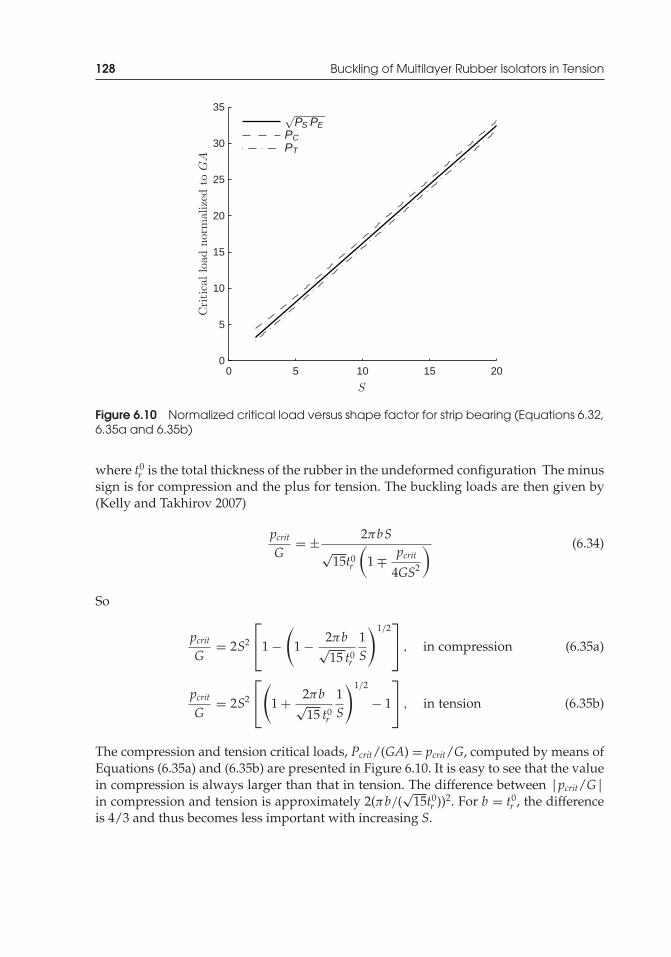
P1: TIX/XYZ P2: ABCJWST069-06 JWST069-Kelly-Style2 July 15, 2011 14:41 Printer Name: Yet to Come
128 Buckling of Multilayer Rubber Isolators in Tension
0 5 10 15 200
5
10
15
20
25
30
35
S
Cri
tica
l lo
ad n
orm
aliz
ed t
o GA
√P PS E
PCPT
Figure 6.10 Normalized critical load versus shape factor for strip bearing (Equations 6.32,6.35a and 6.35b)
where t0r is the total thickness of the rubber in the undeformed configuration The minussign is for compression and the plus for tension. The buckling loads are then given by(Kelly and Takhirov 2007)
pcritG
= ± 2πbS√
15t0r
(1 ∓ pcrit
4GS2
) (6.34)
So
pcritG
= 2S2
⎡⎣1 −
(1 − 2πb√
15 t0r
1S
)1/2⎤⎦ , in compression (6.35a)
pcritG
= 2S2
⎡⎣
(1 + 2πb√
15 t0r
1S
)1/2
− 1
⎤⎦ , in tension (6.35b)
The compression and tension critical loads, Pcrit/(GA) = pcrit/G, computed by means ofEquations (6.35a) and (6.35b) are presented in Figure 6.10. It is easy to see that the valuein compression is always larger than that in tension. The difference between |pcrit/G|in compression and tension is approximately 2(πb/(
√15t0
r ))2. For b = t0r , the difference
is 4/3 and thus becomes less important with increasing S.
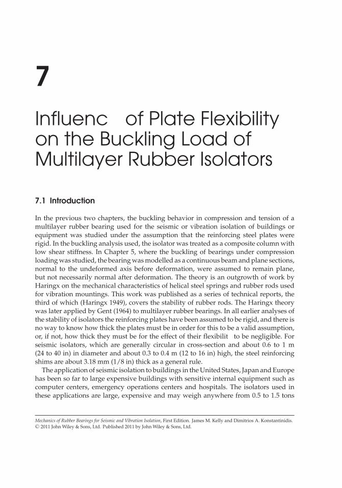
P1: TIX/XYZ P2: ABCJWST069-07 JWST069-Kelly-Style2 July 27, 2011 11:47 Printer Name: Yet to Come
7Influenc of Plate Flexibilityon the Buckling Load ofMultilayer Rubber Isolators
7.1 Introduction
In the previous two chapters, the buckling behavior in compression and tension of amultilayer rubber bearing used for the seismic or vibration isolation of buildings orequipment was studied under the assumption that the reinforcing steel plates wererigid. In the buckling analysis used, the isolator was treated as a composite column withlow shear stiffness. In Chapter 5, where the buckling of bearings under compressionloading was studied, the bearing was modelled as a continuous beam and plane sections,normal to the undeformed axis before deformation, were assumed to remain plane,but not necessarily normal after deformation. The theory is an outgrowth of work byHaringx on the mechanical characteristics of helical steel springs and rubber rods usedfor vibration mountings. This work was published as a series of technical reports, thethird of which (Haringx 1949), covers the stability of rubber rods. The Haringx theorywas later applied by Gent (1964) to multilayer rubber bearings. In all earlier analyses ofthe stability of isolators the reinforcing plates have been assumed to be rigid, and there isno way to know how thick the plates must be in order for this to be a valid assumption,or, if not, how thick they must be for the effect of their flexibilit to be negligible. Forseismic isolators, which are generally circular in cross-section and about 0.6 to 1 m(24 to 40 in) in diameter and about 0.3 to 0.4 m (12 to 16 in) high, the steel reinforcingshims are about 3.18 mm (1/8 in) thick as a general rule.
The application of seismic isolation to buildings in the United States, Japan and Europehas been so far to large expensive buildings with sensitive internal equipment such ascomputer centers, emergency operations centers and hospitals. The isolators used inthese applications are large, expensive and may weigh anywhere from 0.5 to 1.5 tons
Mechanics of Rubber Bearings for Seismic and Vibration Isolation, First Edition. James M. Kelly and Dimitrios A. Konstantinidis.C© 2011 John Wiley & Sons, Ltd. Published 2011 by John Wiley & Sons, Ltd.
129
P1: TIX/XYZ P2: ABCJWST069-07 JWST069-Kelly-Style2 July 27, 2011 11:47 Printer Name: Yet to Come
130 Influenc of Plate Flexibility on the Buckling Load of Multilayer Rubber Isolators
(1.1 to 3.3 kips). There have been efforts to apply this approach to low-cost publichousing in developing countries or poorer regions of developed countries with severeseismic problems. Examples of demonstration projects have been completed in Chile andin the southern Italian region of Reggio Calabria. Demonstration projects with partialsupport from United Nations Industrial Development Organization (UNIDO) were builtin Guangzhou Province, China, and in Indonesia.
To make the seismic isolation useful for such applications, it is necessary to reducethe cost of the isolators and reduce their weight in order to limit the dependence onsite equipment. Both aims can be met either by reducing the thickness of the reinforcingsteel plates or by replacing the steel with a fabric reinforcement, such as carbon fibe(Kelly and Takhirov 2001, Tsai and Kelly 2002). It is possible that flexibilit of the shimsor the lack of bending stiffness in the fibe reinforcement could have a large effect on thebuckling load of a bearing. It is necessary, therefore, to have a theory for the buckling ofthese isolators that takes into account the flexibilit of the reinforcement; such a theorywill be covered in this chapter.
This theory is similar to the compression buckling theory of Chapter 5 in that it treatsthe isolator as a composite beam. The warping of the cross-section, which is permitted bythe flexibilit of the reinforcing sheets, is taken into account by introducing an additionalkinematic displacement function, which will be referred to as the warping function. Itwill be selected to produce no additional rotation of the section, but to measure thedeviation from plane of the deformed cross-section. Force resultants that arise from thepresence of this kinematic quantity are also introduced, and constitutive equations forthese quantities are derived. The appropriate equations of equilibrium incorporatingthese new force quantities are developed: first in the undeformed configuratio fornon-buckling problems; secondly, in the deformed configuratio for buckling problems.
The development of the constitutive equations for rubber bearings is complicated bythe fact that the mechanical response of the thin rubber layers is governed by equationsthat lead to a parabolic stress distribution under pure axial load and a cubic stressdistribution under pure bending (both with zero stress at the free edges), and these haveto be included in the buckling analysis of the isolator.
The outcome of this analysis will include completely rigid plates and completelyflexibl reinforcement as special cases, and it will show that for the typical range of sizesof isolators for buildings, the reduction in buckling load from the completely rigid platecase to the completely flexibl plate case is from 25 to 50%. The analysis will also showthat the 3.18 mm (1/8 in) thick steel plates have almost the same buckling load as thecompletely rigid case, and that 0.79 mm (1/32 in) thick steel plates have almost the samebuckling load as the completely flexibl case. These results are very encouraging forthe design of low-cost isolators and should encourage the development of alternativelightweight reinforcing systems.
7.2 Shearing Deformations of Short Beams
Before developing a theory for the buckling of the isolator with flexibl reinforcingplates, it is useful to develop the theory for a simple beam of rectangular cross-section
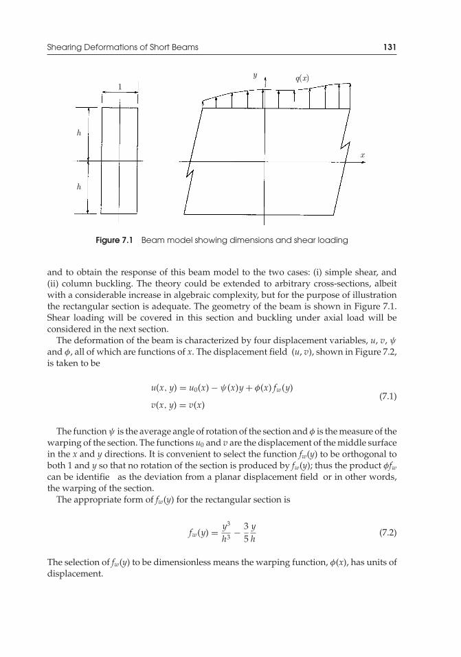
P1: TIX/XYZ P2: ABCJWST069-07 JWST069-Kelly-Style2 July 27, 2011 11:47 Printer Name: Yet to Come
Shearing Deformations of Short Beams 131
Figure 7.1 Beam model showing dimensions and shear loading
and to obtain the response of this beam model to the two cases: (i) simple shear, and(ii) column buckling. The theory could be extended to arbitrary cross-sections, albeitwith a considerable increase in algebraic complexity, but for the purpose of illustrationthe rectangular section is adequate. The geometry of the beam is shown in Figure 7.1.Shear loading will be covered in this section and buckling under axial load will beconsidered in the next section.
The deformation of the beam is characterized by four displacement variables, u, v, ψ
and φ, all of which are functions of x. The displacement field (u, v), shown in Figure 7.2,is taken to be
u(x, y) = u0(x) − ψ(x)y+ φ(x) fw(y)
v(x, y) = v(x)(7.1)
The function ψ is the average angle of rotation of the section and φ is the measure of thewarping of the section. The functions u0 and v are the displacement of the middle surfacein the x and y directions. It is convenient to select the function fw(y) to be orthogonal toboth 1 and y so that no rotation of the section is produced by fw(y); thus the product φfwcan be identifie as the deviation from a planar displacement field or in other words,the warping of the section.
The appropriate form of fw(y) for the rectangular section is
fw(y) = y3
h3 − 35yh
(7.2)
The selection of fw(y) to be dimensionless means the warping function, φ(x), has units ofdisplacement.

P1: TIX/XYZ P2: ABCJWST069-07 JWST069-Kelly-Style2 July 27, 2011 11:47 Printer Name: Yet to Come
132 Influenc of Plate Flexibility on the Buckling Load of Multilayer Rubber Isolators
Figure 7.2 Displacement fiel of beam with shear and warping
The resulting strains are
εxx = u′0 − ψ ′y+ φ′ fw
γxy = (v′ − ψ) + φ f ′w
(7.3)
and assuming elastic behavior, the stresses become
σxx = Eu′0 − Eψ ′y+ Eφ′ fw(y)
τxy = G(v′ − ψ) + Gφ f ′w(y)
(7.4)
We defin a set of stress resultants by
N =∫A
σxxdA (7.5a)
M = −∫A
σxx ydA (7.5b)
Q =∫A
fw(y)σxxdA (7.5c)
V =∫A
τxydA (7.5d)
R =∫A
f ′w(y)τxydA (7.5e)

P1: TIX/XYZ P2: ABCJWST069-07 JWST069-Kelly-Style2 July 27, 2011 11:47 Printer Name: Yet to Come
Shearing Deformations of Short Beams 133
The resultants are related to the kinematic variables by
N = EAu′0 (7.6)
M = E Iψ ′ (7.7)
Q = E J φ′ (7.8)
and
V = GA(v′ − ψ) + GBφ (7.9)
R = GB(v′ − ψ) + GCφ (7.10)
where
A=∫A
dA= 2 h (7.11a)
I =∫A
y2dA= 23h3 (7.11b)
J =∫A
f 2w(y)dA= 8
175h (7.11c)
B =∫A
f ′w(y)dA= 4
5(7.11d)
C =∫A
(f ′w(y)
)2 dA= 4825 h
(7.11e)
Substitution back into the stress equations gives
σxx = NA
− MIy+ Q
Jfw(y)
τxy = CV − BRAC − B2 − BV − AR
AC − B2 f ′w(y)
(7.12)
The equilibrium equations for the stress resultants are derived from the equilibriumequations for the stress, namely
∂σxx
∂x+ ∂τxy
∂y= 0 (7.13)
∂τxy
∂x+ ∂σyy
∂y= 0 (7.14)
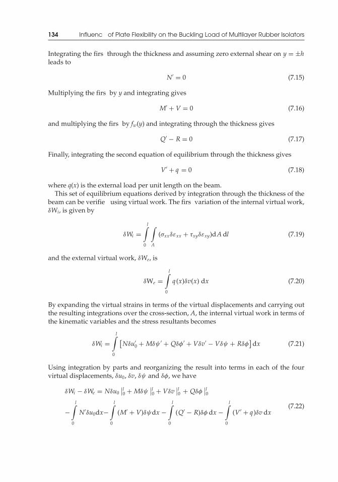
P1: TIX/XYZ P2: ABCJWST069-07 JWST069-Kelly-Style2 July 27, 2011 11:47 Printer Name: Yet to Come
134 Influenc of Plate Flexibility on the Buckling Load of Multilayer Rubber Isolators
Integrating the firs through the thickness and assuming zero external shear on y = ±hleads to
N′ = 0 (7.15)
Multiplying the firs by y and integrating gives
M′ + V = 0 (7.16)
and multiplying the firs by fw(y) and integrating through the thickness gives
Q′ − R = 0 (7.17)
Finally, integrating the second equation of equilibrium through the thickness gives
V′ + q = 0 (7.18)
where q(x) is the external load per unit length on the beam.This set of equilibrium equations derived by integration through the thickness of the
beam can be verifie using virtual work. The firs variation of the internal virtual work,δWi, is given by
δWi =l∫
0
∫A
(σxxδεxx + τxyδεxy)dA dl (7.19)
and the external virtual work, δWe, is
δWe =l∫
0
q (x)δv(x) dx (7.20)
By expanding the virtual strains in terms of the virtual displacements and carrying outthe resulting integrations over the cross-section, A, the internal virtual work in terms ofthe kinematic variables and the stress resultants becomes
δWi =l∫
0
[Nδu′
0 + Mδψ ′ + Qδφ′ + Vδv′ − Vδψ + Rδφ]
dx (7.21)
Using integration by parts and reorganizing the result into terms in each of the fourvirtual displacements, δu0, δv, δψ and δφ, we have
δWi − δWe = Nδu0∣∣l0 + Mδψ
∣∣l0 + Vδv
∣∣l0 + Qδφ
∣∣l0
−l∫
0
N′δu0dx−l∫
0
(M′ + V)δψdx −l∫
0
(Q′ − R)δφ dx −l∫
0
(V′ + q )δv dx(7.22)
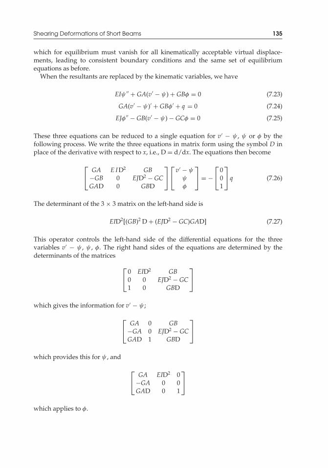
P1: TIX/XYZ P2: ABCJWST069-07 JWST069-Kelly-Style2 July 27, 2011 11:47 Printer Name: Yet to Come
Shearing Deformations of Short Beams 135
which for equilibrium must vanish for all kinematically acceptable virtual displace-ments, leading to consistent boundary conditions and the same set of equilibriumequations as before.
When the resultants are replaced by the kinematic variables, we have
EIψ ′′ + GA(v′ − ψ) + GBφ = 0 (7.23)
GA(v′ − ψ)′ + GBφ′ + q = 0 (7.24)
EJφ′′ − GB(v′ − ψ) − GCφ = 0 (7.25)
These three equations can be reduced to a single equation for v′ − ψ , ψ or φ by thefollowing process. We write the three equations in matrix form using the symbol D inplace of the derivative with respect to x, i.e., D = d/dx. The equations then become
⎡⎣ GA E ID2 GB
−GB 0 EJD2 − GCGAD 0 GBD
⎤⎦
⎡⎣v′ − ψ
ψ
φ
⎤⎦ = −
⎡⎣ 0
01
⎤⎦ q (7.26)
The determinant of the 3 × 3 matrix on the left-hand side is
EID2[(GB)2 D + (EJD2 − GC)GAD] (7.27)
This operator controls the left-hand side of the differential equations for the threevariables v′ − ψ , ψ , φ. The right hand sides of the equations are determined by thedeterminants of the matrices
⎡⎣ 0 EID2 GB
0 0 EJD2 − GC1 0 GBD
⎤⎦
which gives the information for v′ − ψ ;
⎡⎣ GA 0 GB
−GA 0 EJD2 − GCGAD 1 GBD
⎤⎦
which provides this for ψ , and
⎡⎣ GA EID2 0
−GA 0 0GAD 0 1
⎤⎦
which applies to φ.
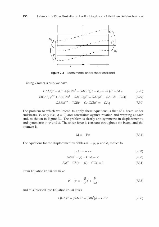
P1: TIX/XYZ P2: ABCJWST069-07 JWST069-Kelly-Style2 July 27, 2011 11:47 Printer Name: Yet to Come
136 Influenc of Plate Flexibility on the Buckling Load of Multilayer Rubber Isolators
Figure 7.3 Beam model under shear end load
Using Cramer’s rule, we have
GAEJ(v′ − ψ)′′′ + [(GB)2 − GAGC](v′ − ψ) = −EJq′′ + GCq (7.28)
EIGAEJψ ′′′′ + EI[(GB)2 − GAGC]ψ ′′ = GAEJq′′ + GA(GB− GC)q (7.29)
GAEJφ′′′′ + [(GB)2 − GAGC]φ′′ = −GAq (7.30)
The problem to which we intend to apply these equations is that of a beam underendshears, V, only (i.e., q = 0) and constraints against rotation and warping at eachend, as shown in Figure 7.3. The problem is clearly anti-symmetric in displacement vand symmetric in ψ and φ. The shear force is constant throughout the beam, and themoment is
M = −Vx (7.31)
The equations for the displacement variables, v′ − ψ , ψ and φ, reduce to
EIψ ′ = −Vx (7.32)
GA(v′ − ψ) + GBφ = V (7.33)
EJφ′′ − GB(v′ − ψ) − GCφ = 0 (7.34)
From Equation (7.33), we have
v′ − ψ = − BA
φ + VGA
(7.35)
and this inserted into Equation (7.34) gives
EJGAφ′′ − [GAGC− (GB)2]φ = GBV (7.36)
P1: TIX/XYZ P2: ABCJWST069-07 JWST069-Kelly-Style2 July 27, 2011 11:47 Printer Name: Yet to Come
Shearing Deformations of Short Beams 137
The alternative form in terms of (v′ − ψ) is
EJGA(v′ − ψ)′′ − [GAGC− (GB)2](v′ − ψ) = −GCV (7.37)
We note that the combination AC − B2 for the rectangular section is positive, so that thesolutions are hyperbolic functions. The solutions are
φ = C1 cosh (ωx) − GBGAGC− (GB)2V
and
v′ − ψ = D1 cosh (ωx) − GCGAGC− (GB)2V
where
ω2 = GAGC− (GB)2
EJGA(7.38)
and where C1 and D1 are related through Equation (7.35) as
D1 cosh(ωx) + CAC− B2
VG
= − BA
(C1 cosh(ωx) − B
AC− B2
VG
)+ VGA
i.e.,
D1 = − BAC1 (7.39)
The boundary conditions at x = ±l require that both ψ and φ vanish, and this deter-mines that
φ(x) = − BAC− B2
(1 − cosh (ωx)
cosh (ωl)
)VG
(7.40)
and
v′ − ψ = VGA
(AC
AC− B2 − B2
AC− B2
cosh (ωx)cosh (ωl)
)(7.41)
From Equation (7.32), we have
ψ = − V2EI
x2 + C3
and since ψ (±l) = 0
ψ = V2EI
(l2 − x2) (7.42)
P1: TIX/XYZ P2: ABCJWST069-07 JWST069-Kelly-Style2 July 27, 2011 11:47 Printer Name: Yet to Come
138 Influenc of Plate Flexibility on the Buckling Load of Multilayer Rubber Isolators
To complete the solution, we substitute for ψ in Equation (7.41) and integrate, obtaining
v(x) = V2EI
(l2x − x3
3
)− VGA
(B2
AC− B2
1ω
sinh (ωx)cosh (ωl)
− ACAC− B2 x
)(7.43)
where we have set v(0) = 0 to maintain the anti-symmetry of the solution for v(x). Thedeflection at each end are ±δ where
δ = Vl3
3EI+ VlGA
(AC
AC− B2 − B2
AC− B2
tanh(ωl)ωl
)(7.44)
For the rectangular section considered here
ACAC− B2 = 6
5(7.45)
and
B2
AC− B2 = 15
(7.46)
so that if we suppress the warping by setting E J → ∞, i.e., φ everywhere zero, thenωl → 0, and δs, the part of δ due to shear, becomes
δs → VlGA
(7.47)
On the other hand, to model the case when there is no restraint on the warping at theend of the beam, the warping stiffness EJ is set to zero, then
λl → ∞ and δs → 65VlGA
= Vl
G(
5A6
) (7.48)
which corresponds to the usual theory of shear deformation in beams. Furthermore, ifφ is not constrained and either EJ → 0 or alternatively φ ′′ → 0, then
φ = − BC
(v′ − ψ) (7.49)
and
τxy = G(
1 − BCf ′w(y)
)(v′ − ψ) (7.50)
which with Equation (7.12) gives
τxy = 3V2 A
(1 − y2
h2
)(7.51)
P1: TIX/XYZ P2: ABCJWST069-07 JWST069-Kelly-Style2 July 27, 2011 11:47 Printer Name: Yet to Come
Buckling of Short Beams with Warping Included 139
Thus, if the effect of the warping is not included, the solution reduces to the standardbeam theory with shear deformation included. The influenc of the constraint of thewarping depends on the parameter ωl, which is given by
(ωl)2 = GEAC− B2
JAl2 = 35G
El2
h2 (7.52)
It follows that ω is likely to be large, and the solution for φ(x) near x = ±l can bewritten as
φ(x) = − ABAC− B2 [1 − e−ω(l−x)]
VGA
(7.53)
We can defin a penetration length l p for the distance over which the constraint of thewarping is important by setting ωl p = 1, which gives l p ≈ h/3.5. Clearly this means thatthe constraint of the warping is of no significanc in normal beams. The effective E inisolators is of the order of several hundred times G and, in such cases, the constraintof the warping at the ends will be effective over much larger distances from the ends.Before turning to the equivalent isolator problem, however, in the next section we willconsider the buckling problem for this beam example.
7.3 Buckling of Short Beams with Warping Included
The main problem associated with the determination of the buckling load for the shortbeam with shear and warping included, is the determination of the appropriate equi-librium equations in the buckled configuration Since we have no physically intuitiveunderstanding of Q and R, a direct method is not available and a formal approach mustbe used, such as that which led to Q′ − R = 0. To verify the results of the formal approach,we can compare it to the form of the equilibrium equations in Chapter 5 on compressionbuckling, where plane sections remain plane, which corresponds to EJ → ∞ and φ → 0,in which case an intuitive approach is possible.
To develop the equations of equilibrium that correspond to Equations (5.2a) and (5.2b)in Chapter 5 when the warping variables Q and R are included, we resort to integrationof the stress equations of equilibrium through the thickness.
We consider a differential element of the material with sides dx and dy in the un-deformed configuratio parallel and perpendicular to the undeformed beam axis asshown in Figure 7.4. In the deformed configuration the edges of the element parallel tothe x-axis are parallel to the deformed middle surface of the beam and the edges parallelto the y-axis are rotated through the angles θ and θ + (∂θ/∂x) dx, where θ is the localrotation of the vertical line element given by
θ = −∂u∂y
= ψ − φ f ′w(y) (7.54)
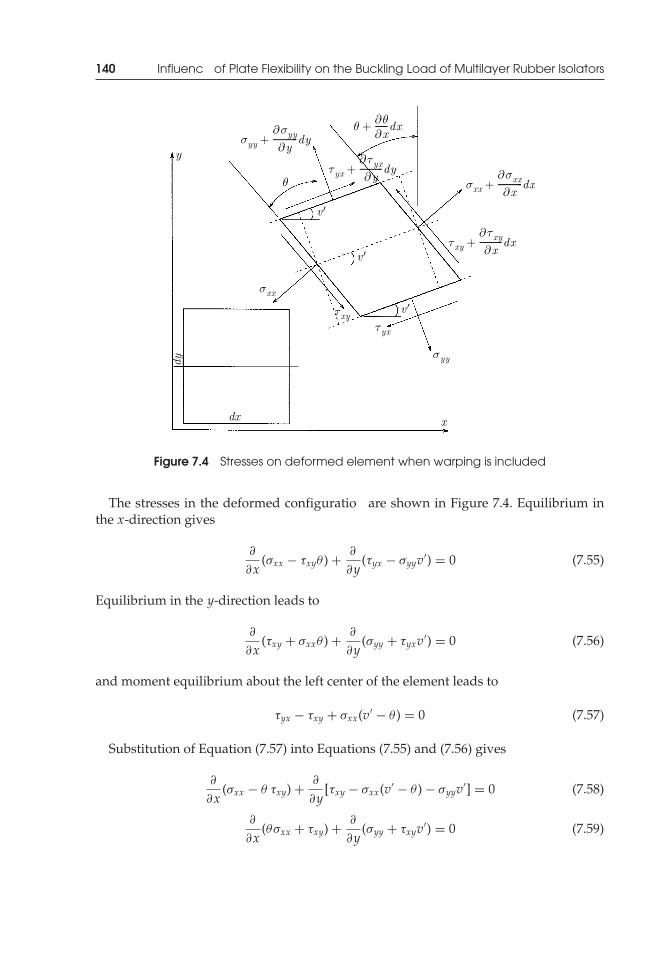
P1: TIX/XYZ P2: ABCJWST069-07 JWST069-Kelly-Style2 July 27, 2011 11:47 Printer Name: Yet to Come
140 Influenc of Plate Flexibility on the Buckling Load of Multilayer Rubber Isolators
Figure 7.4 Stresses on deformed element when warping is included
The stresses in the deformed configuratio are shown in Figure 7.4. Equilibrium inthe x-direction gives
∂
∂x(σxx − τxyθ ) + ∂
∂y(τyx − σyyv′) = 0 (7.55)
Equilibrium in the y-direction leads to
∂
∂x(τxy + σxxθ ) + ∂
∂y(σyy + τyxv′) = 0 (7.56)
and moment equilibrium about the left center of the element leads to
τyx − τxy + σxx(v′ − θ ) = 0 (7.57)
Substitution of Equation (7.57) into Equations (7.55) and (7.56) gives
∂
∂x(σxx − θ τxy) + ∂
∂y[τxy − σxx(v′ − θ ) − σyyv′] = 0 (7.58)
∂
∂x(θσxx + τxy) + ∂
∂y(σyy + τxyv′) = 0 (7.59)
P1: TIX/XYZ P2: ABCJWST069-07 JWST069-Kelly-Style2 July 27, 2011 11:47 Printer Name: Yet to Come
Buckling of Short Beams with Warping Included 141
Integration of both equations over the cross-section −h ≤ y ≤ h and assuming traction-free surfaces at y = ±h leads to
dNdx
= 0 (7.60)
ddx
(Nψ − NB
Aφ + V
)= 0 (7.61)
Multiplication of the firs by y and integration over the cross-section leads to
dMdx
+ V − N(v′ − ψ) − NABφ = 0 (7.62)
Multiplication of the firs by fw(y) and integration over the cross-section leads to
dQdx
− R+ NAB(v′ − ψ) + N
ACφ = 0 (7.63)
These equations of equilibrium in the deformed configuration developed by integrationover the cross-sectional area of the equations of stress equilibrium can be verifie asbefore by the use of virtual work. However when the stability of the beam model isconsidered, it is necessary to include length changes due to second-order effects. Thelateral displacement of the beam, v(x) causes an increase in length of any horizontalplane that depends on the slope v′(x) in the form
ε1 dx = (1 − cos v′) dx = 12v′2dx (7.64)
and the shear deformation causes a reduction in length
ε2 dx = (1 − cos γxy) dx = 12γ 2xy dx (7.65)
These two terms contribute to the internal virtual work δWi such that the f rst variationof the internal virtual work becomes
δ Wi =l∫
0
∫A
{σxx
[δ
(12v′2
)− δ
(12γ 2xy
)]}dA dx +
l∫0
∫A
(σxxδεxx + τxyδεxy) dA dl
(7.66)
The firs integral can be written as
I1 =l∫
0
∫A
(σxxv′δv′ − σxxγxyδγxy) dA dx (7.67)
P1: TIX/XYZ P2: ABCJWST069-07 JWST069-Kelly-Style2 July 27, 2011 11:47 Printer Name: Yet to Come
142 Influenc of Plate Flexibility on the Buckling Load of Multilayer Rubber Isolators
which with γxy = v′ − ψ + φ f ′w and δγxy = δv′ − δψ + δφ f ′
w means that
γxyδγxy = v′δv′ − ψδv′ + φ f ′wδv′ − v′δψ + ψδψ − φ f ′
wδψ + v′ f ′wδφ
−ψ f ′wδφ + φ f ′
wδφ (7.68)
and from this, the firs integral becomes
I1 =l∫
0
[(NBA
φ − Nψ
)δv′ +
(Nψ − NB
Aφ − Nv′
)δψ +
(NBAv′ − NB
Aψ + NB
Aφ
)δφ
]dx
(7.69)The second integral becomes
I2 =l∫
0
(Nδu′0 + Mδψ ′ + Qδφ′ + Vδv′ − Vδψ + Rδφ) dx (7.70)
Adding the two integrals together and using integration by parts in the usual way, thefirs variation of the virtual work takes the form
I1 + I2 = Nδu0∣∣l0 +
(−Nψ + NB
Aφ + V
)δv
∣∣l0 + Mδψ
∣∣l0 +
l∫0
N′δu0 dx
+l∫
0
[(−Nψ + NB
Aφ
)′+ V′
]δv dx +
l∫0
(−Nv′ + Nψ − NB
Aφ − M′ − V
)δψ dx
+l∫
0
(−NB
Av′ + NB
Aψ − NC
Aφ − Q′ + R
)δφdx (7.71)
It is easy to see that this expression leads to the same equations of equilibrium as beforeand also provides the appropriate boundary conditions for the beam.
The firs equation, Equation (7.60), reduces to
N = −P (7.72)
Integration of Equation (7.61) gives
V − P(
ψ − BA
φ
)= −H0 (7.73)
and when this is inserted into Equation (7.62), it can be integrated to give
M+ Pv = H0x + M0 + Pv0 (7.74)
P1: TIX/XYZ P2: ABCJWST069-07 JWST069-Kelly-Style2 July 27, 2011 11:47 Printer Name: Yet to Come
Buckling of Short Beams with Warping Included 143
If we set φ = 0, i.e., θ = ψ , then the set of equilibrium equations reduces to the systemof Equations (5.2a) and (5.2b), derived by direct application of equilibrium. When theconstitutive equations are used, the equilibrium equations become
EIψ ′ + Pv = H0x + M0 + Pv0 (7.75)
GA(v′ − ψ) +(G + P
A
)Bφ − Pψ = −H0 (7.76)
EJφ′′ −(G + P
A
)B(v′ − ψ) −
(G + P
A
)Cφ = 0 (7.77)
These three equations can be reduced to a single equation for φ or ψ by the followingprocess. We write the three equations in matrix form, using the symbol D in place of thederivative with respect to x, i.e. D = d/dx. The equations then become
⎡⎢⎢⎢⎣
P EID 0
GAD −(GA+ P) (GA+ P)BA
−(GA+ P)BA
D (GA+ P)BA
EJD2 − (GA+ P)CA
⎤⎥⎥⎥⎦
⎡⎣ v
ψ
φ
⎤⎦ =
⎡⎣H0x + M0 + Pv0
−H0
0
⎤⎦
(7.78)
The determinant of the 3 × 3 matrix on the left-hand side is
P(GA+ P)2CA
− P(GA+ P)EJD2 − EI(GA+ P)2 B2
A2 D2 − P(GA+ P)2 B2
A2
+EIGA(GA+ P)CA
D2 − EIGAEJD4 (7.79)
This operator controls the left hand side of the differential equations for the three vari-ables v, ψ, φ. The right hand sides of the equations are determined by the determinantsof the matrices
⎡⎢⎢⎢⎣H0x + M0 + Pv0 EID 0
−H0 −(GA+ P) (GA+ P)BA
0 (GA+ P)BA
EJD2 − (GA+ P)CA
⎤⎥⎥⎥⎦
which gives the information for v;
⎡⎢⎢⎢⎣
P H0x + M0 + Pv0 0
GAD −H0 (GA+ P)BA
−(GA+ P)BA
D 0 EJD2 − (GA+ P)CA
⎤⎥⎥⎥⎦
P1: TIX/XYZ P2: ABCJWST069-07 JWST069-Kelly-Style2 July 27, 2011 11:47 Printer Name: Yet to Come
144 Influenc of Plate Flexibility on the Buckling Load of Multilayer Rubber Isolators
which provides this for ψ , and⎡⎢⎣
P EID H0x + M0 + Pv0
GAD −(GA+ P) −H0
−(GA+ P)BA
D (GA+ P)BA
0
⎤⎥⎦
which applies to φ.Using Cramer’s rule, we have
EJGAEId4
dx4
⎡⎣ v
ψ
φ
⎤⎦ +
[EJ(GA+ P)P + EI(GA+ P)2 B
2
A2 − GAEI(GA+ P)CA
]d2
dx2
⎡⎣ v
ψ
φ
⎤⎦
+[
(GA+ P)2 B2
A2 P − (GA+ P)2PCA
] ⎡⎣ v
ψ
φ
⎤⎦ =
⎡⎢⎢⎢⎢⎢⎢⎢⎢⎣
(GA+ P)2
[(BA
)2
− CA
](H0x + M0 + Pv0)
(GA+ P)2
[(BA
)2
− CA
]H0
0
⎤⎥⎥⎥⎥⎥⎥⎥⎥⎦
(7.80)
As before, we take H0 = 0 and ψ = cos(πx/(2l)) to satisfy the constraints at x = ±land determine the buckling load P from
EJGAEIπ4
4 l4−
[EJ
(G + P
A
)AP+ EI
(G + P
A
)2
B2 − GAEI(G + P
A
)C
]π2
4 l2
+(G + P
A
)2
(B2 − AC) P = 0 (7.81)
It is convenient to defin the following dimensionless quantities:
(i) the normalized buckling load:
p = PGA
(7.82)
(ii) the normalized column geometry:
λ = πh2l
(7.83)
(iii) the normalized stiffnesses:
k1 = GB2h2
EAJk2 = GAh2
EI(7.84)
P1: TIX/XYZ P2: ABCJWST069-07 JWST069-Kelly-Style2 July 27, 2011 11:47 Printer Name: Yet to Come
Buckling of Short Beams with Warping Included 145
and the parameter γ = AC/B2 in terms of which Equation (7.81) becomes
λ4 − {k1[(1 + p)2 − γ (1 + p)] + k2 p(1 + p)}λ2 + k1k2 p(1 + p)2(1 − γ ) = 0 (7.85)
It is useful to factor this into the form
{λ2 − k1[(1 + p)2 − γ (1 + p)]}[λ2 − k2 p(1 + p)] − k1k2 p2(1 + p)2 = 0 (7.86)
We note that if k1 → 0, i.e., EJ → ∞, or no warping, we have
λ2 = k2 p(1 + p) (7.87)
which is the same result as we had in Chapter 5 for the buckling with no warping; andif k2 → 0, i.e., EJ → ∞ (no rotation, ψ ≡ 0), we have
λ2 = k1[(1 + p)2 − γ (1 + p)] (7.88)
Furthermore, if the quantity γ is allowed to become very large (although in this case itis fixe at 6), we see that
λ2 → k2 p(1 + p) (7.89)
Another possible case is EI = 0 and EJ → 0, which corresponds to the buckling of abeam with no restraint on warping. In this case, k1 → ∞, and if we divide by k1, we have
λ2 = k2 p(1 + p)2(1 − γ )(1 + p)2 − γ (1 + p)
= 5 k2 p(1 + p)5 − p
(7.90)
In this case, as λ → 0, p → λ2/k2, i.e.,
PGA
→ π2EI4l2
(7.91)
and as λ → ∞,
P → 5GA (7.92)
The solution for p in terms of λ for the complete solution and the various special casesis shown in Figure 7.5 using the parameters E = 2.5G and the values of A, B, C, I, J, asgiven in Section 7.2. A comparison of the values of p for the case where φ = 0 and thefull equation shows that neglecting warping can greatly overestimate the buckling load.Comparison of the case when the warping is unconstrained, i.e., EJ → 0, shows thatneglecting the end constraints against warping can greatly underestimate the load. Ithas to be emphasized, of course, that these results are of very little practical applicationto real beams since it is almost certain that for most materials the value of the buckling
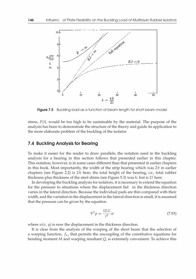
P1: TIX/XYZ P2: ABCJWST069-07 JWST069-Kelly-Style2 July 27, 2011 11:47 Printer Name: Yet to Come
146 Influenc of Plate Flexibility on the Buckling Load of Multilayer Rubber Isolators
Figure 7.5 Buckling load as a function of beam length for short beam model
stress, P/A, would be too high to be sustainable by the material. The purpose of theanalysis has been to demonstrate the structure of the theory and guide its application tothe more elaborate problem of the buckling of the isolator.
7.4 Buckling Analysis for Bearing
To make it easier for the reader to draw parallels, the notation used in the bucklinganalysis for a bearing in this section follows that presented earlier in this chapter.This notation, however, is in some cases different than that presented in earlier chaptersin this book. Most importantly, the width of the strip bearing which was 2 b in earlierchapters (see Figure 2.2) is 2 h here; the total height of the bearing, i.e., total rubberthickness plus thickness of the steel shims (see Figure 5.3) was h, but is 2 l here.
In developing the buckling analysis for isolators, it is necessary to extend the equationfor the pressure to situations where the displacement fiel in the thickness directionvaries in the lateral direction. Because the individual pads are thin compared with theirwidth, and the variation in the displacement in the lateral direction is small, it is assumedthat the pressure can be given by the equation
∇2 p = 12Gt3 w (7.93)
where w(x, y) is now the displacement in the thickness direction.It is clear from the analysis of the warping of the short beam that the selection of
a warping function, fw , that permits the uncoupling of the constitutive equations forbending moment M and warping resultant Q, is extremely convenient. To achieve this
P1: TIX/XYZ P2: ABCJWST069-07 JWST069-Kelly-Style2 July 27, 2011 11:47 Printer Name: Yet to Come
Buckling Analysis for Bearing 147
for an isolator when the stress in the axial direction is obtained from Equation (7.93) byreplacing p by −σxx and w/t by εxx, we need to select fw(y) such that
∫A
σxx ydA (7.94)
is independent of φ(x), and
∫A
σxx fw(y) dA (7.95)
is independent of ψ(x) when σxx is given by
∇2σxx = −12Gt2 εxx (7.96)
A suitable selection of fw(y) is
fw(y) = y3
h3 − 37yh
(7.97)
and with this, we have
u(x, y) = u(x) − ψ(x)y+ φ(x)(y3
h3 − 37yh
)(7.98)
v(x, y) = v(x) (7.99)
from which
εxx = u′ − ψ ′(x)y+ φ′(x)(y3
h3 − 37yh
)(7.100)
The equation for σxx becomes
d2σxx
dy2 = −12Gt2
[u′ − ψ ′y+ φ′
(y3
h3 − 37yh
)](7.101)
and with σxx = 0 at y = ±h, this leads to
σxx = −6Gt2 h2
(y2
h2 − 1)u′ + 2G
t2 h3(y3
h3 − yh
)ψ ′ − 12Gh2
20 t2
(y5
h5 − 107y3
h3 + 37yh
)φ′
(7.102)
P1: TIX/XYZ P2: ABCJWST069-07 JWST069-Kelly-Style2 July 27, 2011 11:47 Printer Name: Yet to Come
148 Influenc of Plate Flexibility on the Buckling Load of Multilayer Rubber Isolators
With the previous definition of M and Q, this leads to
N = 4Gh2
t2 hu′ = EAu′ (7.103)
M = 8Gh2
15 t2 h3ψ ′ = EIψ ′ (7.104)
Q = 2Gh2
1225 t2 hφ′ = EJφ′ (7.105)
We calculate the other resultants from
τxy = G(v′ − ψ
) + Gφ3h
(y2
h2 − 17
)(7.106)
obtaining as before
V = GA(v′ − ψ
) + GBφ (7.107)
R = GB(v′ − ψ
) + GCφ (7.108)
where now
A= 2 h (7.109a)
B = 2421
(7.109b)
C = 552245 h
(7.109c)
The structure of the theory for non-buckling problems is now exactly the same asbefore with the values of the nominal EI and EJ being given in terms of G and the shapefactor of a single layer, S = h/t, which may be quite large.
For the pure shear of an isolator in the absence of vertical load, the characteristiclength of penetration of the restraint produced by the boundary condition at the ends ofthe bearing, which for the short beam model was
l p ≈√
E35 g
h (7.110)
is now given by
(λl p
)2 = 1 (7.111)
where
(λl p
)2 = GAGC− (GB)2
EJGAl2p (7.112)
P1: TIX/XYZ P2: ABCJWST069-07 JWST069-Kelly-Style2 July 27, 2011 11:47 Printer Name: Yet to Come
Buckling Analysis for Bearing 149
with
EJ = 2Gh3
1225t2 (7.113)
Thus
(λlp
)2 = 980l2pt
2
h2h2 (7.114)
giving
lp ≈ h30
ht
≈ S30h (7.115)
In this case, the penetration length is of the same order as the width of the bearing.When we turn to the buckling problem, it is necessary to have the stress distribution of
σxx due to the axial load N, denoted here by σ axx. From Equation (7.96) and the boundary
conditions on σxx at y = ±h we have
σ axx = 3N
4 h
(1 − y2
h2
)(7.116)
The equations of equilibrium in the deformed configuratio are as before
∂
∂x(σxx − θτ xy
) + ∂
∂y(τxy − σxx
(v′ − θ
) − σyyv′) = 0 (7.117)
∂
∂x(θσ xx + τxy
) + ∂
∂y(σyy + τxyv′) = 0 (7.118)
with
θ = ψ − φ f ′w (y) (7.119)
The same process of integration of the firs through the thickness when it is multipliedby 1, y, and fw(y), and the use of σ a
xx as given above, leads to
ddx
N = 0 (7.120)
ddx
(V + Nψ − N
ABφ
)= 0 (7.121)
ddx
M+ V − N(v′ − ψ
) − NABφ = 0 (7.122)
ddx
Q− R+ NAB
(v′ − ψ
) + NACφ = 0 (7.123)

P1: TIX/XYZ P2: ABCJWST069-07 JWST069-Kelly-Style2 July 27, 2011 11:47 Printer Name: Yet to Come
150 Influenc of Plate Flexibility on the Buckling Load of Multilayer Rubber Isolators
These are the same as before with the difference that the parabolic stress distribution forσ axx leads to the modificatio of B and C . The constants B and C are given by
B =h∫
−h
32
(1 − y2
h2
)f ′w (y) dy = 12
35(7.124)
and
C =h∫
−h
32
(1 − y2
h2
)f ′2w (y) dy = 216
245 h(7.125)
Returning to Figure 5.2, which shows the generic beam element with end loads, settingN = −P and integrating Equation (7.121) gives
V − Pψ + PABφ = −H0 (7.126)
When this is used to eliminate V from Equation (7.122), we obtain
M′ + Pv′ = H0 (7.127)
which, when integrated, gives
M+ Pv = H0x + M0 + Pv0 (7.128)
and when the constitutive relationships for the force resultants are used, the completesystem becomes
EIψ ′ + Pv = H0 + M0 + Pv0 (7.129)
GA(v′ − ψ
) + GB
(1 + P
GABB
)φ − Pψ = −H0 (7.130)
EJφ′′ − GB
(1 + P
GABB
) (v′ − ψ
) − GC
(1 + P
GACC
)φ = 0 (7.131)
Proceeding as before to reduce these to a single equation in ψ , we obtain
EIEJGAψ ′′′′ +[EJ
(G + P
A
)AP+ EI
(G + P
AB
2
B
)B2 − GA
(G + P
ACC
)C
]ψ ′′
+⎡⎣
(G + P
ABB
)2
+(G + P
A
)A
(G + P
ACC
)C
⎤⎦ Pψ =
[(G + P
A
)2
−(G + P
A
)AC
]H0
(7.132)
P1: TIX/XYZ P2: ABCJWST069-07 JWST069-Kelly-Style2 July 27, 2011 11:47 Printer Name: Yet to Come
Buckling Analysis for Bearing 151
As before, we take ψ = cos(πx/(2l)) and H0 = 0, as shown in Figure 5.2, and obtain asthe equation for P
EIEJGAπ4
16 l4−
⎡⎣EJ
(G + P
A
)AP+ EI
(G + P
ABB
)2
B2 − GA
(G + P
ACC
)C
⎤⎦ π2
4l2
+P
⎡⎣
(G + P
ABB
)2
−(G + P
A
)A
(G + P
ACC
)C
⎤⎦ = 0 (7.133)
In this case, it is convenient to use the same set of normalized quantities as earlier,namely,
p = PGA
(7.134a)
λ = πh2l
(7.134b)
k1 = GB2h2
EAJ(7.134c)
k2 = GAh2
EI(7.134d)
γ = ACB2 (7.134e)
and to add α = B/B, β = C/C in terms of which the equation for relating p and λ
becomes
λ4 −{k1
[(1 + αp)2 − γ (1 + βp)
]+ k2 p (1 + p)
}λ2
+k1k2 p[(1 + αp)2 − γ (1 + βp) (1 + p)
]= 0
(7.135)
In the derivation so far it has been assumed that the steel reinforcing plates arecompletely flexibl and provide no resistance to the warping of the cross-section. Toinclude the effect of the plates, it is useful to consider the various terms that contributeto the elastic stored energy of the deformation. These are
(i) bending
12Mψ ′ = 1
2EIψ ′2 (7.136)
(ii) warping
12Qφ′ = 1
2E J φ′2 (7.137)

P1: TIX/XYZ P2: ABCJWST069-07 JWST069-Kelly-Style2 July 27, 2011 11:47 Printer Name: Yet to Come
152 Influenc of Plate Flexibility on the Buckling Load of Multilayer Rubber Isolators
(iii) shear
12V
(v′ − ψ
) + 12Rφ = 1
2GA
(v′ − ψ
)2 + GB(v′ − ψ
)φ + 1
2GCφ2 (7.138)
When the plates are bent into the shape φ(x) fw(y), they add to the stored energy aterm Wp (per unit width) of the form
Wp = 12
Ept3p12
(1 − ν2
p
)φ2 (x)
h∫−h
(f ′′w y
)2 dy (7.139)
where Ep and vp are the Young’s modulus and Poisson’s ratio of the plate material andtp is the plate thickness. For the present form of fw this becomes
Wp = Ept3p(
1 − ν2p
) 1h3 φ2 (7.140)
This contribution must be divided by t + tp to reduce it to energy per unit width per unitlength, and is then added to GCφ2/2. Thus, the term C in Equation (7.133) is replaced byC∗ where
C∗ = C + 2 Ep
G(1 − ν2
p
) t2ph3
1t + tp
(7.141)
From the initial definitio of C (Equation 7.109c) we have C = 552/(245h), thus
C∗ = C
(1 + 490
552Ep
G(1 − ν2
p
) t3p
h2
1t + tp
)(7.142)
The fina form of the equation for p in terms of λ is
λ4 −{k1
[(1 + αp)2 − γ (1 + βp)
]+ k2 p (1 + p)
}λ2
+ k1k2 p[(1 + αp)2 − γ (1 + βp) (1 + p)
]= 0
(7.143)
where
γ = AC∗
B2 (7.144)
The solution of this equation for the normalized buckling load as a function of theaspect ratio of the bearing, λ, can be obtained for different values of the reinforcing platethickness. Examples will be given in the next section.
P1: TIX/XYZ P2: ABCJWST069-07 JWST069-Kelly-Style2 July 27, 2011 11:47 Printer Name: Yet to Come
Computation of Buckling Loads 153
7.5 Computation of Buckling Loads
In order to use the analysis for the buckling of short uniform beams as a guide in thedevelopment of the buckling load for the isolator, it was useful to retain the notation EIand EJ for the bending and warping stiffnesses of the isolator. At this point, it is moreconvenient to have them expressed in terms of the isolation geometry as follows.
In terms of the half width, h, and the rubber layer thickness, t, we have
EI = 8Gh5
15 t2 (7.145)
and
EJ = 2Gh3
1225 t2(7.146)
from which with
A= 2 h (7.147a)
B = 2421
(7.147b)
C = 552245 h
(7.147c)
k1 = GB2h2
E J A= 400
S2 (7.147d)
k2 = GAh2
EI= 15
4 S2 (7.147e)
where S is the shape factor of a single layer. The other parameters are
α = BB
= 310
(7.148a)
β = CC
= 923
(7.148b)
γ = ACB2 = 3.45 (7.148c)
and
γ = γ
(1 + 490
552Ep
G(1 − ν2
p
) t2p
h2
tp1 + tp
)(7.148d)
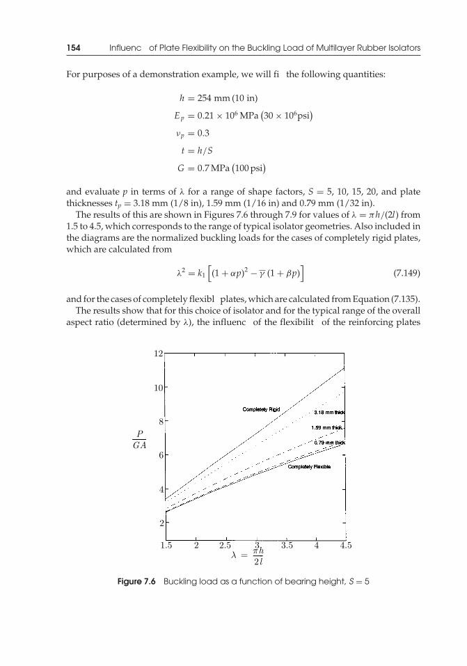
P1: TIX/XYZ P2: ABCJWST069-07 JWST069-Kelly-Style2 July 27, 2011 11:47 Printer Name: Yet to Come
154 Influenc of Plate Flexibility on the Buckling Load of Multilayer Rubber Isolators
For purposes of a demonstration example, we will fi the following quantities:
h = 254 mm (10 in)
Ep = 0.21 × 10⁶ MPa(30 × 106psi
)νp = 0.3
t = h/S
G = 0.7 MPa(100 psi
)
and evaluate p in terms of λ for a range of shape factors, S = 5, 10, 15, 20, and platethicknesses tp = 3.18 mm (1/8 in), 1.59 mm (1/16 in) and 0.79 mm (1/32 in).
The results of this are shown in Figures 7.6 through 7.9 for values of λ = πh/(2l) from1.5 to 4.5, which corresponds to the range of typical isolator geometries. Also included inthe diagrams are the normalized buckling loads for the cases of completely rigid plates,which are calculated from
λ2 = k1
[(1 + αp)2 − γ (1 + βp)
](7.149)
and for the cases of completely flexibl plates, which are calculated from Equation (7.135).The results show that for this choice of isolator and for the typical range of the overall
aspect ratio (determined by λ), the influenc of the flexibilit of the reinforcing plates
Figure 7.6 Buckling load as a function of bearing height, S = 5
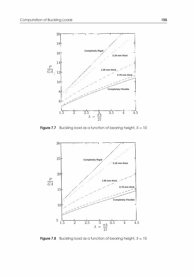
P1: TIX/XYZ P2: ABCJWST069-07 JWST069-Kelly-Style2 July 27, 2011 11:47 Printer Name: Yet to Come
Computation of Buckling Loads 155
Completely Rigid
Completely Flexible
3.18 mm thick
1.59 mm thick
0.79 mm thick
Figure 7.7 Buckling load as a function of bearing height, S = 10
Completely Rigid
Completely Flexible
1.59 mm thick
3.18 mm thick
0.79 mm thick
Figure 7.8 Buckling load as a function of bearing height, S = 15
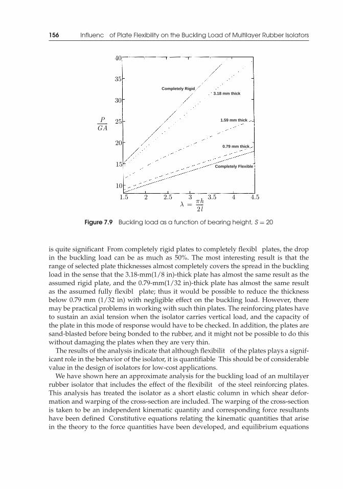
P1: TIX/XYZ P2: ABCJWST069-07 JWST069-Kelly-Style2 July 27, 2011 11:47 Printer Name: Yet to Come
156 Influenc of Plate Flexibility on the Buckling Load of Multilayer Rubber Isolators
Completely Rigid
Completely Flexible
1.59 mm thick
3.18 mm thick
0.79 mm thick
Figure 7.9 Buckling load as a function of bearing height, S = 20
is quite significant From completely rigid plates to completely flexibl plates, the dropin the buckling load can be as much as 50%. The most interesting result is that therange of selected plate thicknesses almost completely covers the spread in the bucklingload in the sense that the 3.18-mm(1/8 in)-thick plate has almost the same result as theassumed rigid plate, and the 0.79-mm(1/32 in)-thick plate has almost the same resultas the assumed fully flexibl plate; thus it would be possible to reduce the thicknessbelow 0.79 mm (1/32 in) with negligible effect on the buckling load. However, theremay be practical problems in working with such thin plates. The reinforcing plates haveto sustain an axial tension when the isolator carries vertical load, and the capacity ofthe plate in this mode of response would have to be checked. In addition, the plates aresand-blasted before being bonded to the rubber, and it might not be possible to do thiswithout damaging the plates when they are very thin.
The results of the analysis indicate that although flexibilit of the plates plays a signif-icant role in the behavior of the isolator, it is quantifiable This should be of considerablevalue in the design of isolators for low-cost applications.
We have shown here an approximate analysis for the buckling load of an multilayerrubber isolator that includes the effect of the flexibilit of the steel reinforcing plates.This analysis has treated the isolator as a short elastic column in which shear defor-mation and warping of the cross-section are included. The warping of the cross-sectionis taken to be an independent kinematic quantity and corresponding force resultantshave been defined Constitutive equations relating the kinematic quantities that arisein the theory to the force quantities have been developed, and equilibrium equations
P1: TIX/XYZ P2: ABCJWST069-07 JWST069-Kelly-Style2 July 27, 2011 11:47 Printer Name: Yet to Come
Computation of Buckling Loads 157
have been obtained in the undeformed configuratio for non-buckling problems, andin the deformed configuratio for the buckling problem. Although the theory has beendeveloped for the problem of the buckling of the isolator, a by-product of the analysis isthe buckling analysis of short elastic beams of uniform configuratio in which shear andwarping are taken into account. Of course, the influenc of shear and warping on thebuckling loads of regular beams will not be very important or of practical application,except in extremely short beams where the stresses would be extremely high, and elasticbuckling would probably not apply.
The results show that the influenc of warping can be significan for typically sizedisolators and for the typical height-to-width ratio. It also shows that to provide an isolatorwith a buckling load that is negligibly reduced from that obtained from the usual theorywith assumed rigid plates, the plates thickness need not be greater than 3.18 mm (1/8 in),and that if the plate thickness is reduced to less than 0.79 mm (1/32 in), there is only anegligible further reduction in the buckling load.
There is increasing interest in several developing countries to use rubber isolatorsin the earthquake-resistant design of public housing and other local facilities, such asschools and hospitals. For these isolators to be cost-effective in these applications, it willbe essential to reduce the steel content, both to reduce cost and to reduce weight toobviate the use of lifting equipment. The results of this analysis show that this shouldbe possible, and this should lead to increased use of this potentially valuable technologyin earthquake-prone regions of the developing world.

P1: TIX/XYZ P2: ABCJWST069-07 JWST069-Kelly-Style2 July 27, 2011 11:47 Printer Name: Yet to Come

P1: TIX/XYZ P2: ABCJWST069-08 JWST069-Kelly-Style2 July 27, 2011 1:16 Printer Name: Yet to Come
8Frictional Restraint onUnbonded Rubber Pads
8.1 Introduction
In Chapter 1 we referred to the patent by the French engineer Eugene Freyssinet on hisproposal (1954) for the use of multilayer rubber bearings as bridge supports and hissuggestions of several types of steel reinforcement for these bearings. In his patent, it isclear that he envisaged that the rubber layers and the steel plates could be held togetheronly by friction, and in fact he indicated that he thought that friction would be a morereliable method than gluing the rubber and steel together. He also thought, correctly,that the pressure would rise from zero at the edge of a bearing to a maximum at thecenter, but, mistakenly, that the shear stress between the rubber and steel also variedfrom zero at the edge to a maximum at the center. We saw in Chapter 2 that this is notthe case.
This raises the question as to what the result of using friction and only friction tohold the bearing together can mean for the device. In this chapter, we will examine thisthrough two special cases, namely the long strip pad and the circular pad. The analysisis an extension of the pressure solution for a fully bonded pad, and it will show thatthe results of Chapter 2 must be modifie if friction is the connecting process, but alsothat at the high levels of friction that can be attained between rubber and steel, the effectof slip between the rubber and the steel is not very significant In the next chapter, wewill describe a theory for a type of unbonded multilayer bearing that is held in place byfriction and show test results on such a bearing.
The material in Sections 8.2 and 8.3 firs appeared in the article by Kelly, J. M. and Konstantinidis, D. (2009).“Effect of Friction on Unbonded Elastomeric Bearings.” Journal of Engineering Mechanics (ASCE), 135(9),953–960. DOI 10.1061/(ASCE)EM.1943-7889.0000019. Reproduced with permission from ASCE.
Mechanics of Rubber Bearings for Seismic and Vibration Isolation, First Edition. James M. Kelly and Dimitrios A. Konstantinidis.C© 2011 John Wiley & Sons, Ltd. Published 2011 by John Wiley & Sons, Ltd.
159

P1: TIX/XYZ P2: ABCJWST069-08 JWST069-Kelly-Style2 July 27, 2011 1:16 Printer Name: Yet to Come
160 Frictional Restraint on Unbonded Rubber Pads
8.2 Compression of Long Strip Pad with Frictional Restraint
In this section we are only interested in the theory for a pad in the form of a longstrip when the effects of the ends can be neglected, and the strip is taken to be infiniteThe theory for an arbitrarily shaped pad is given in Chapter 2, and the importantpoints applicable to the analysis of a long strip pad are repeated here for the reader’sconvenience. We consider a pad of thickness t and width 2b and locate a rectangularCartesian coordinate system, (x, y, z), in the middle surface of the pad, as shown inFigure 8.1(a). Figure 8.1(b) shows the displacements, (u,w), in the coordinate directionsunder the following assumptions: (i) points on a vertical line before deformation lie ona parabola after loading, and (ii) horizontal planes remain horizontal,
u(x, z) = u0(x)(
1 − 4 z2
t2
)
w(x, z) = w(z)(8.1)
This displacement fiel satisfie the constraint that the top and bottom surfaces of thepad are bonded to rigid substrates. The assumption of incompressibility produces afurther constraint on the normal components of strain, εxx, εzz, in the form
εxx + εzz = ∂u∂x
+ ∂w∂z
= du0
dx
(1 − 4 z2
t2
)+ dw
dz= 0 (8.2)
Figure 8.1 Infinitel long rectangular pad showing dimensions
P1: TIX/XYZ P2: ABCJWST069-08 JWST069-Kelly-Style2 July 27, 2011 1:16 Printer Name: Yet to Come
Compression of Long Strip Pad with Frictional Restraint 161
When integrated through the thickness, this gives
du0
dx= 3
2�
t= 3
2εc (8.3)
where � is the change of thickness (� > 0 in compression), and εc = �/t is the compres-sion strain.
The other assumptions of the theory are that the material is incompressible and that thestress state is dominated by the pressure p in the sense that the normal stress componentscan be taken as –p. The vertical shear stress components are included in the analysis,but the in-plane shear stress is assumed to be negligible. The only equation of stressequilibrium in this case is
∂σxx
∂x+ ∂τxz
∂z= 0 (8.4)
which with the assumption that σ xx = σ zz = –p provides the sole equation of equilibrium
∂τxz
∂z= dp
dx(8.5)
The assumption of linear elastic behavior means that
τxz = Gγxz = G(
∂u∂z
+ ∂w∂x
)= −8G
t2zu0 (8.6)
This equation together with (8.3) and (8.5) leads to
d2 pdx2 = −12Gεc
t2 (8.7)
The boundary condition at the edges of the pad, p(x= ±b) = 0, completes the system forthe pressure distribution, p(x). The solution is given by
p (x) = 6Gεc
t2
(b2 − x2) = 6GS2εc
(1 − x2
b2
)(8.8)
since S= b/t. The effective compression modulusEc of the pad is obtained by integratingp(x) over the area of the pad to determine the resultant load P, i.e., the load per unitlength of the strip. The effective compression modulus Ec is then given by
Ec = PAεc
= 12 bεc
b∫−b
p (x) dx = 4GS2 (8.9)
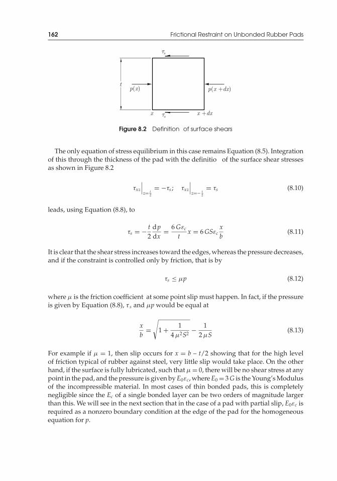
P1: TIX/XYZ P2: ABCJWST069-08 JWST069-Kelly-Style2 July 27, 2011 1:16 Printer Name: Yet to Come
162 Frictional Restraint on Unbonded Rubber Pads
t
s
s
p(x) p(x +dx)
x x +dx
Figure 8.2 Definition of surface shears
The only equation of stress equilibrium in this case remains Equation (8.5). Integrationof this through the thickness of the pad with the definitio of the surface shear stressesas shown in Figure 8.2
τxz
∣∣∣z= t
2
= −τs ; τxz
∣∣∣z=− t
2
= τs (8.10)
leads, using Equation (8.8), to
τs = − t2
dpdx
= 6Gεc
tx = 6GSεc
xb
(8.11)
It is clear that the shear stress increases toward the edges, whereas the pressure decreases,and if the constraint is controlled only by friction, that is by
τs ≤ μp (8.12)
where μ is the friction coefficient at some point slip must happen. In fact, if the pressureis given by Equation (8.8), τ s and μp would be equal at
xb
=√
1 + 14 μ2S2 − 1
2 μS(8.13)
For example if μ = 1, then slip occurs for x = b – t/2 showing that for the high levelof friction typical of rubber against steel, very little slip would take place. On the otherhand, if the surface is fully lubricated, such that μ = 0, there will be no shear stress at anypoint in the pad, and the pressure is given byE0εc, whereE0 = 3G is the Young’s Modulusof the incompressible material. In most cases of thin bonded pads, this is completelynegligible since the Ec of a single bonded layer can be two orders of magnitude largerthan this. We will see in the next section that in the case of a pad with partial slip, E0εc isrequired as a nonzero boundary condition at the edge of the pad for the homogeneousequation for p.
P1: TIX/XYZ P2: ABCJWST069-08 JWST069-Kelly-Style2 July 27, 2011 1:16 Printer Name: Yet to Come
The Effect of Surface Slip on the Vertical Stiffness of an Infinit Strip Pad 163
8.3 The Effect of Surface Slip on the Vertical Stiffnessof an Infinit Strip Pad
In order to accommodate the slip at the surface due to the shear stresses overcomingthe frictional resistance between the rubber and the steel or concrete, we need to modifythe original kinematic assumptions. In this approach, as before, the rubber is assumedincompressible and the pressure is assumed to be the dominant stress component.The kinematic assumption of quadratically variable displacement is supplemented byan additional displacement that is constant through the thickness and is intended toaccommodate the squeezing out of the rubber where slip occurs, as shown in Figure 8.3.Thus, in this case the displacement pattern that leads to the pressure solution of Equation(8.8) is replaced by the displacement fiel
u (x, z) = u0 (x)(
1 − 4 z2
t2
)+ u1 (x)
w (x, z) = w (z)
(8.14)
where u1(x) = 0 for 0 ≤ x ≤ x1, with x1 being the location where slip starts.The constraint of incompressibility consistent with the displacement pattern of Equa-
tion (8.14) leads to
du0
dx+ 3
2du1
dx= 3
2�
t= 3
2εc (8.15)
The only equation of stress equilibrium in this case is
∂σxx
∂x+ ∂τxz
∂z= 0 (8.16)
and the assumption of elastic behavior means that
τxz = Gγxz (8.17)
Figure 8.3 Coordinate system and displacement field for a single, infinitel long strip padwith slip
P1: TIX/XYZ P2: ABCJWST069-08 JWST069-Kelly-Style2 July 27, 2011 1:16 Printer Name: Yet to Come
164 Frictional Restraint on Unbonded Rubber Pads
which, with
γxz = ∂u∂z
+ ∂w∂x
= − 8t2 zu0 (8.18)
from Equation (8.14), gives
∂σxx
∂x= 8G
t2 u0 (8.19)
which, with the assumption that σ xx = σ zz = −p, provides the sole equation ofequilibrium as
dpdx
= −8Gt2 u0 (8.20)
In the region where no slip has occurred, i.e. 0 ≤ x ≤ x1, the slip displacement is zeroand Equation (8.20) can be inverted to give u0 in terms of pressure and inserted into theincompressibility constraint (Equation 8.15), to give
p (x) = −6Gεc
t2 x2 + Ax + B
Symmetry implies that A = 0, giving
p (x) = −6Gεc
t2 x2 + B
It is convenient to absorb the unknown constant into the other constants and write thepressure as
p (x) = 6Gεcb2
t2
(B − x2
b2
)= 6GS2εc
(B − x2
b2
)(8.21)
For x1 ≤ x≤ b, we need to determine u1(x) subject to the simultaneous requirements thatτ s = μp and τ s = –(t/2) dp/dx. This leads to the equation
dpdx
+ 2 μ
tp = 0 (8.22)
which has solution p(x) = Ce−2μx/t, where C is a constant of integration. To determineit, we use as boundary condition at x = b the fact that p(b) = E0εc = 3Gεc. Thus forx1 ≤ x ≤ b, the pressure is given by
p (x) = −3Gεce (2μ/t)(b−x) (8.23)
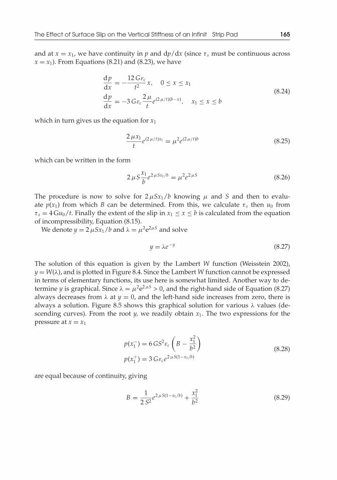
P1: TIX/XYZ P2: ABCJWST069-08 JWST069-Kelly-Style2 July 27, 2011 1:16 Printer Name: Yet to Come
The Effect of Surface Slip on the Vertical Stiffness of an Infinit Strip Pad 165
and at x = x1, we have continuity in p and dp/dx (since τ s must be continuous acrossx = x1). From Equations (8.21) and (8.23), we have
dpdx
= −12Gεc
t2x, 0 ≤ x ≤ x1
dpdx
= −3Gεc2 μ
te (2 μ/t)(b−x), x1 ≤ x ≤ b
(8.24)
which in turn gives us the equation for x1
2 μx1
te (2 μ/t)x1 = μ2e (2 μ/t)b (8.25)
which can be written in the form
2 μSx1
be2 μSx1/b = μ2e2 μS (8.26)
The procedure is now to solve for 2 μSx1/b knowing μ and S and then to evalu-ate p(x1) from which B can be determined. From this, we calculate τ s then u0 fromτ s = 4 Gu0/t. Finally the extent of the slip in x1 ≤ x ≤ b is calculated from the equationof incompressibility, Equation (8.15).
We denote y = 2 μSx1/b and λ = μ2e2μS and solve
y = λe−y (8.27)
The solution of this equation is given by the Lambert W function (Weisstein 2002),y=W(λ), and is plotted in Figure 8.4. Since the LambertW function cannot be expressedin terms of elementary functions, its use here is somewhat limited. Another way to de-termine y is graphical. Since λ = μ2e2 μS > 0, and the right-hand side of Equation (8.27)always decreases from λ at y = 0, and the left-hand side increases from zero, there isalways a solution. Figure 8.5 shows this graphical solution for various λ values (de-scending curves). From the root y, we readily obtain x1. The two expressions for thepressure at x = x1
p(x−1 ) = 6GS2εc
(B − x2
1
b2
)
p(x+1 ) = 3Gεce2 μS(1−x1/b)
(8.28)
are equal because of continuity, giving
B = 12 S2 e
2 μS(1−x1/b) + x21
b2 (8.29)
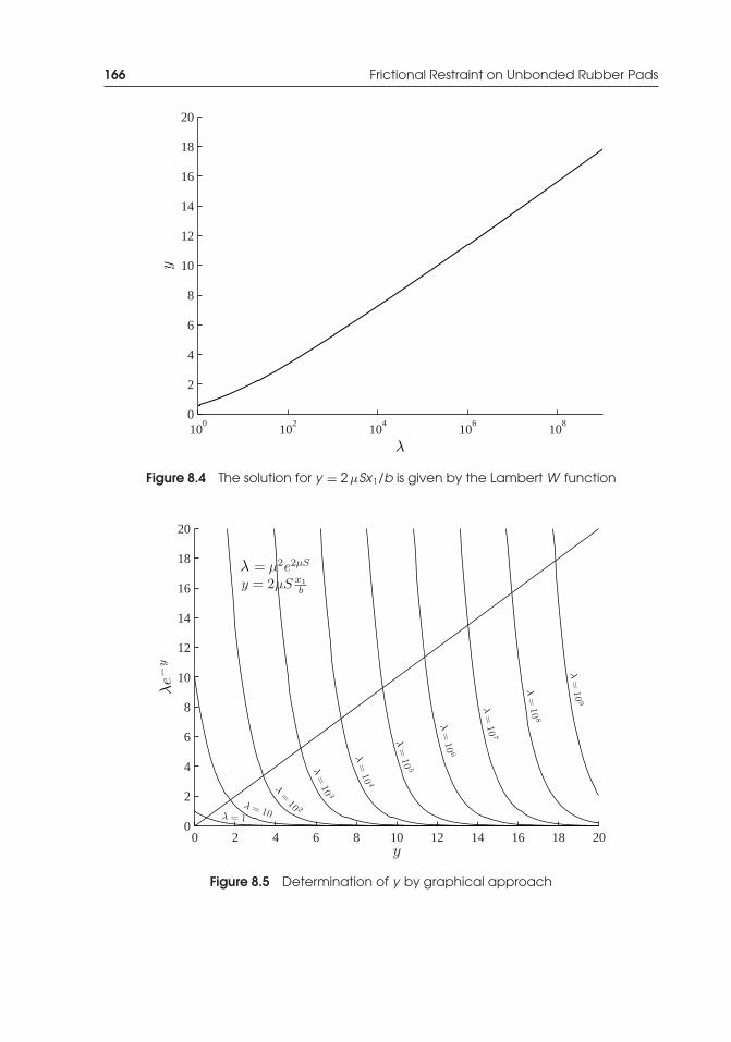
P1: TIX/XYZ P2: ABCJWST069-08 JWST069-Kelly-Style2 July 27, 2011 1:16 Printer Name: Yet to Come
166 Frictional Restraint on Unbonded Rubber Pads
100
102
104
106
108
0
2
4
6
8
10
12
14
16
18
20
y
λ
Figure 8.4 The solution for y = 2 μSx1/b is given by the Lambert W function
0 2 4 6 8 10 12 14 16 18 200
2
4
6
8
10
12
14
16
18
20
−y
y
= 10= 1
=10 2
=10 3
=10
4
=10
5
=10
6
=10
7
=10
8
=10
9
= μ2e2µS
y = 2μS x1b
λ
λe
λλ
λ
λ
λ
λ
λ
λ
λ
λ
Figure 8.5 Determination of y by graphical approach
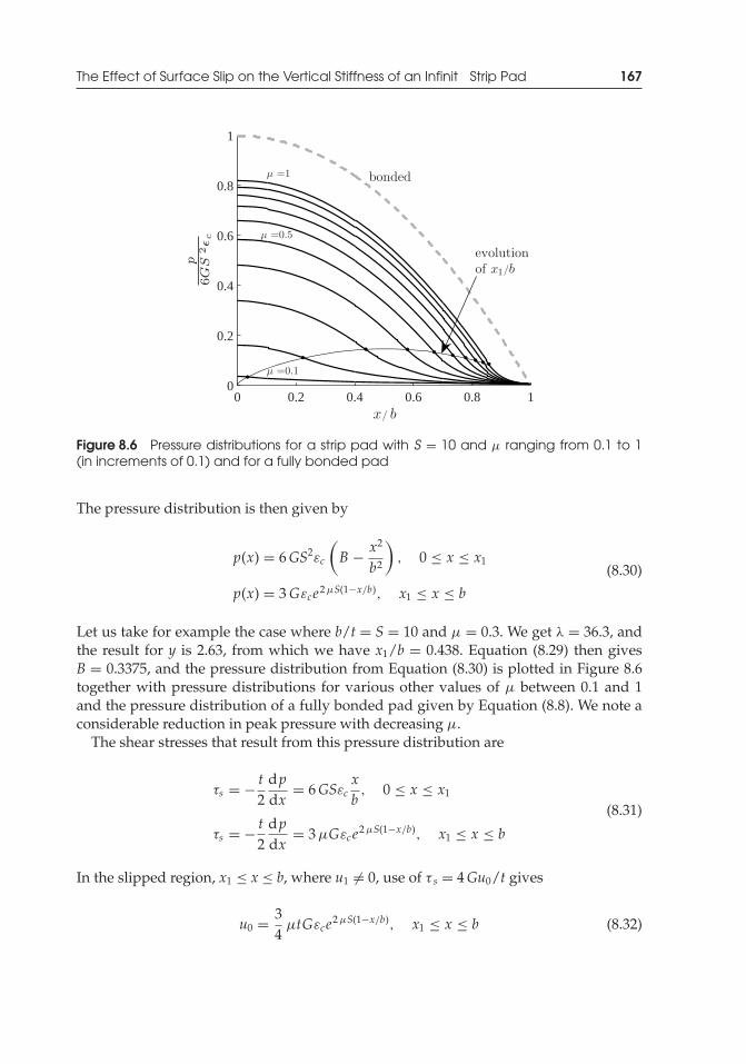
P1: TIX/XYZ P2: ABCJWST069-08 JWST069-Kelly-Style2 July 27, 2011 1:16 Printer Name: Yet to Come
The Effect of Surface Slip on the Vertical Stiffness of an Infinit Strip Pad 167
0 0.2 0.4 0.6 0.8 10
0.2
0.4
0.6
0.8
1
x/ b
p6GS
2c
evolutionof x1/b
μ =0.1
μ =0.5
μ =1 bonded
Figure 8.6 Pressure distributions for a strip pad with S = 10 and μ ranging from 0.1 to 1(in increments of 0.1) and for a fully bonded pad
The pressure distribution is then given by
p(x) = 6GS2εc
(B − x2
b2
), 0 ≤ x ≤ x1
p(x) = 3Gεce2 μS(1−x/b), x1 ≤ x ≤ b
(8.30)
Let us take for example the case where b/t = S = 10 and μ = 0.3. We get λ = 36.3, andthe result for y is 2.63, from which we have x1/b = 0.438. Equation (8.29) then givesB = 0.3375, and the pressure distribution from Equation (8.30) is plotted in Figure 8.6together with pressure distributions for various other values of μ between 0.1 and 1and the pressure distribution of a fully bonded pad given by Equation (8.8). We note aconsiderable reduction in peak pressure with decreasing μ.
The shear stresses that result from this pressure distribution are
τs = − t2
dpdx
= 6GSεcxb, 0 ≤ x ≤ x1
τs = − t2
dpdx
= 3 μGεce2 μS(1−x/b), x1 ≤ x ≤ b
(8.31)
In the slipped region, x1 ≤ x ≤ b, where u1 �= 0, use of τ s = 4Gu0/t gives
u0 = 34
μtGεce2 μS(1−x/b), x1 ≤ x ≤ b (8.32)
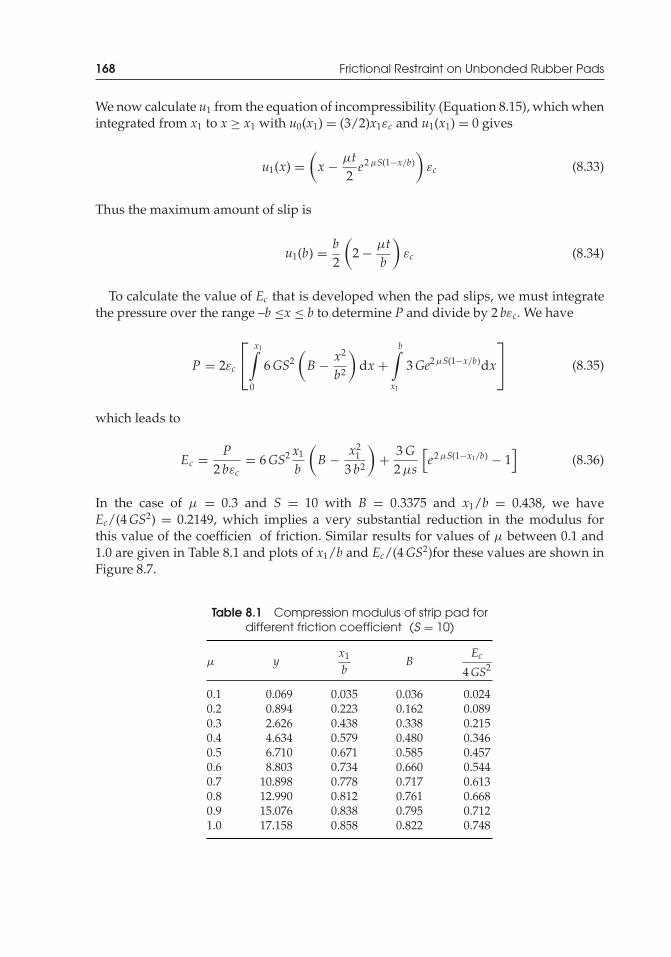
P1: TIX/XYZ P2: ABCJWST069-08 JWST069-Kelly-Style2 July 27, 2011 1:16 Printer Name: Yet to Come
168 Frictional Restraint on Unbonded Rubber Pads
We now calculate u1 from the equation of incompressibility (Equation 8.15), which whenintegrated from x1 to x ≥ x1 with u0(x1) = (3/2)x1εc and u1(x1) = 0 gives
u1(x) =(x − μt
2e2 μS(1−x/b)
)εc (8.33)
Thus the maximum amount of slip is
u1(b) = b2
(2 − μt
b
)εc (8.34)
To calculate the value of Ec that is developed when the pad slips, we must integratethe pressure over the range –b ≤x ≤ b to determine P and divide by 2 bεc. We have
P = 2εc
⎡⎣
x1∫0
6GS2(B − x2
b2
)dx +
b∫x1
3Ge2 μS(1−x/b)dx
⎤⎦ (8.35)
which leads to
Ec = P2 bεc
= 6GS2 x1
b
(B − x2
1
3 b2
)+ 3G
2 μs
[e2 μS(1−x1/b) − 1
](8.36)
In the case of μ = 0.3 and S = 10 with B = 0.3375 and x1/b = 0.438, we haveEc/(4GS2) = 0.2149, which implies a very substantial reduction in the modulus forthis value of the coefficien of friction. Similar results for values of μ between 0.1 and1.0 are given in Table 8.1 and plots of x1/b and Ec/(4GS2)for these values are shown inFigure 8.7.
Table 8.1 Compression modulus of strip pad fordifferent friction coefficient (S = 10)
μ yx1
bB
Ec4GS2
0.1 0.069 0.035 0.036 0.0240.2 0.894 0.223 0.162 0.0890.3 2.626 0.438 0.338 0.2150.4 4.634 0.579 0.480 0.3460.5 6.710 0.671 0.585 0.4570.6 8.803 0.734 0.660 0.5440.7 10.898 0.778 0.717 0.6130.8 12.990 0.812 0.761 0.6680.9 15.076 0.838 0.795 0.7121.0 17.158 0.858 0.822 0.748
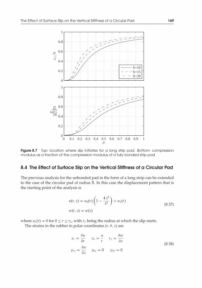
P1: TIX/XYZ P2: ABCJWST069-08 JWST069-Kelly-Style2 July 27, 2011 1:16 Printer Name: Yet to Come
The Effect of Surface Slip on the Vertical Stiffness of a Circular Pad 169
0
0.2
0.4
0.6
0.8
1
x1/b
0 0.1 0.2 0.3 0.4 0.5 0.6 0.7 0.8 0.9 10
0.2
0.4
0.6
0.8
1
Ec
4GS
2
μ
S=10S=15S=20
Figure 8.7 Top: location where slip initiates for a long strip pad. Bottom: compressionmodulus as a fraction of the compression modulus of a fully bonded strip pad
8.4 The Effect of Surface Slip on the Vertical Stiffness of a Circular Pad
The previous analysis for the unbonded pad in the form of a long strip can be extendedto the case of the circular pad of radius R. In this case the displacement pattern that isthe starting point of the analysis is
u(r, z) = u0(r )(
1 − 4 z2
t2
)+ u1(r )
w(r, z) = w(z)
(8.37)
where u1(r) = 0 for 0 ≤ r ≤ r1, with r1 being the radius at which the slip starts.The strains in the rubber in polar coordinates (r, θ, z) are
εr = ∂u∂r
εθ = ur
εz = ∂w∂z
γrz = ∂u∂z
γθz = 0 γrθ = 0(8.38)
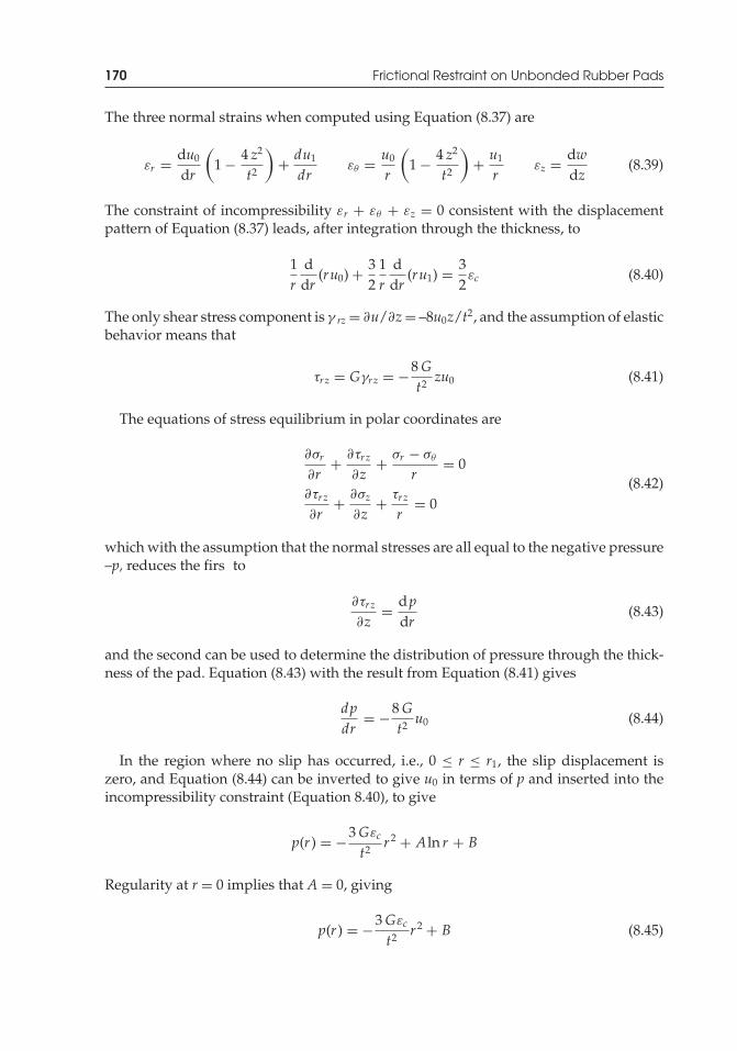
P1: TIX/XYZ P2: ABCJWST069-08 JWST069-Kelly-Style2 July 27, 2011 1:16 Printer Name: Yet to Come
170 Frictional Restraint on Unbonded Rubber Pads
The three normal strains when computed using Equation (8.37) are
εr = du0
dr
(1 − 4 z2
t2
)+ du1
drεθ = u0
r
(1 − 4 z2
t2
)+ u1
rεz = dw
dz(8.39)
The constraint of incompressibility εr + εθ + εz = 0 consistent with the displacementpattern of Equation (8.37) leads, after integration through the thickness, to
1r
ddr
(ru0) + 32
1r
ddr
(ru1) = 32εc (8.40)
The only shear stress component is γ rz = ∂u/∂z= –8u0z/t2, and the assumption of elasticbehavior means that
τrz = Gγrz = −8Gt2 zu0 (8.41)
The equations of stress equilibrium in polar coordinates are
∂σr
∂r+ ∂τrz
∂z+ σr − σθ
r= 0
∂τrz
∂r+ ∂σz
∂z+ τrz
r= 0
(8.42)
which with the assumption that the normal stresses are all equal to the negative pressure–p, reduces the firs to
∂τrz
∂z= dp
dr(8.43)
and the second can be used to determine the distribution of pressure through the thick-ness of the pad. Equation (8.43) with the result from Equation (8.41) gives
dpdr
= −8Gt2
u0 (8.44)
In the region where no slip has occurred, i.e., 0 ≤ r ≤ r1, the slip displacement iszero, and Equation (8.44) can be inverted to give u0 in terms of p and inserted into theincompressibility constraint (Equation 8.40), to give
p(r ) = −3Gεc
t2 r2 + Aln r + B
Regularity at r = 0 implies that A = 0, giving
p(r ) = −3Gεc
t2 r2 + B (8.45)

P1: TIX/XYZ P2: ABCJWST069-08 JWST069-Kelly-Style2 July 27, 2011 1:16 Printer Name: Yet to Come
The Effect of Surface Slip on the Vertical Stiffness of a Circular Pad 171
It is convenient to absorb the unknown constant into the other constants and write thepressure as
p(r ) = 3GεcR2
t2
(B − r 2
R2
)(8.46)
If there were no slip anywhere, we could use p(R) = 0 to determine B and getp(r) = (3Gεc/t2)(R2 – r2), which is the same result we obtained in Chapter 2 for thebonded circular pad. It is convenient to express this in terms of the shape factor S,whichfor the circular pad is R/(2t), with which Equation (8.46) becomes
p(r ) = 12GS2εc
(B − r2
R2
)(8.47)
The maximum value of the pressure when there is no slip is 12GS2εc which we will uselater for comparison purposes.
For x1 ≤ r ≤ R, we need to determine u1(r) subject to the simultaneous requirementsthat τ s = μp and τ s = –(t/2)dp/dr. This leads to the equation
dpdr
+ 2 μ
tp = 0 (8.48)
This equation has the solution p(r) = Ce−2 μr/t, where C is a constant of integration. Todetermine it, we use as the boundary condition at r= R the fact that p(R) = E0εc = 3Gεc.Thus for r1 ≤ r ≤ R, the pressure is given by
p(r ) = 3Gεce (2 μ/t)(R−r ) (8.49)
and at r = r1, we have continuity in p and dp/dr (since τ s must be continuous r = r1).Differentiating Equations (8.46) and (8.49) and equating them, we obtain
dpdr
∣∣∣∣r=r1
= −6Gt2 r1εc = −3Gεc
(2 μ
t
)e(2 μ/t)(R−r1) (8.50)
which in turn gives
2 μr1
te (2 μ/t)r1 = 2 μ2e (2 μ/t)R (8.51)
or, in terms of S,
4 μSr1
Re4 μSr1/R = 2 μ2e4 μS (8.52)
Letting y = 4 μSr1/R and λ = 2 μ2e4μS, this equation reduces to
y = λe−y (8.53)
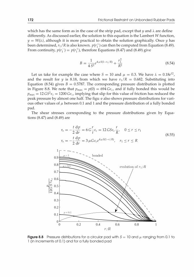
P1: TIX/XYZ P2: ABCJWST069-08 JWST069-Kelly-Style2 July 27, 2011 1:16 Printer Name: Yet to Come
172 Frictional Restraint on Unbonded Rubber Pads
which has the same form as in the case of the strip pad, except that y and λ are definedifferently. As discussed earlier, the solution to this equation is the Lambert W function,y = W(λ), although it is more practical to obtain the solution graphically. Once y hasbeen determined, r1/R is also known. p(r+
1 ) can then be computed from Equation (8.49).From continuity, p(r−
1 ) = p(r+1 ), therefore Equations (8.47) and (8.49) give
B = 14 S2 e
4 μS(1−r1/R) + r21
R2 (8.54)
Let us take for example the case where S = 10 and μ = 0.3. We have λ = 0.18e12,and the result for y is 8.18, from which we have r1/R = 0.682. Substituting intoEquation (8.54) gives B = 0.5787. The corresponding pressure distribution is plottedin Figure 8.8. We note that pmax = p(0) = 694Gεc, and if fully bonded this would bepmax = 12GS2εc = 1200Gεc, implying that slip for this value of friction has reduced thepeak pressure by almost one half. The figu e also shows pressure distributions for vari-ous other values of μ between 0.1 and 1 and the pressure distribution of a fully bondedpad.
The shear stresses corresponding to the pressure distributions given by Equa-tions (8.47) and (8.49) are
τs = − t2
dpdr
= 6Grtεc = 12GSεc
rR
, 0 ≤ r ≤ r1
τs = − t2
dpdr
= 3 μGεce4 μS(1−r/R), r1 ≤ r ≤ R(8.55)
0 0.2 0.4 0.6 0.8 10
0.1
0.2
0.3
0.4
0.5
0.6
0.7
0.8
0.9
1
r/R
p12GS
2c
bondedμ = 1
μ = 0.1
μ = 0.5 evolution of r1/R
Figure 8.8 Pressure distributions for a circular pad with S = 10 and μ ranging from 0.1 to1 (in increments of 0.1) and for a fully bonded pad
P1: TIX/XYZ P2: ABCJWST069-08 JWST069-Kelly-Style2 July 27, 2011 1:16 Printer Name: Yet to Come
The Effect of Surface Slip on the Vertical Stiffness of a Circular Pad 173
In the slipped region, r1 ≤ r ≤ R, where u1 �= 0, use of τ s = 4Gu0/t gives
u0 = 34
μtεce4 μS(1−r/R), r1 ≤ r ≤ R (8.56)
We now calculate u1 from the equation of incompressibility (Equation 8.40), which whenintegrated from to r1 to r ≥ r1 with u0(r1) = (3/4) r1εc and u1(r1) = 0 gives
u1(r ) = εc
2
(r − μte4 μS(1−r/R)
), r1 ≤ r ≤ R (8.57)
Thus the maximum amount of slip is
u1(R) = εc
2(R− μt) (8.58)
To calculate the value of Ec that is developed when the pad slips we must integratethe pressure over the range 0 ≤ r ≤ R to determine P and divide by Aεc = πR2εc. Wehave,
P = 2πεc
⎡⎣
r1∫0
12GS2(B − r2
R2
)rdr +
R∫r1
3Ge4 μS(1−r/R)rdr
⎤⎦ (8.59)
which leads to
Ec6GS2 =
r1∫0
4(B − r2
R2
)rR2 dr +
R∫r1
1S2 e
4 μS(1−r/R) rR2 dr (8.60)
The result is
Ec6GS2 = 2B
r 21
R2 − r41
R4 + 1S2
(1 + 4 μSr1/R) e4 μS(1−r1/R) − (1 + 4 μS)(4 μS)2 (8.61)
In the case of μ = 0.3 and S = 10 with B = 0.5787 and r1/R = 0.682, we haveEc/(6GS2) = 0.350, which implies a significan reduction in the modulus for this valueof friction coefficient Similar results for values of μ between 0.1 and 1.0 are given inTable 8.2 and plots of r1/R and Ec/(6GS2) for these values are shown in Figure 8.9.
The analysis in this chapter has concentrated on a single pad, either long strip orcircular, that is held in place between rigid surfaces only by friction. One purpose of thishas been to quantify the suggestion of Freyssinet that friction might be more reliablethan gluing the rubber to steel when constructing a multilayer bearing. He seemed notto be confiden in the glues that were available for this purpose at that time. Of coursethe subsequent development of bonding compounds with very reliable properties haseliminated this concern. There may, however, be a few situations where unbonded singlelayers are used in technical applications.
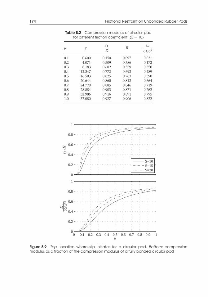
P1: TIX/XYZ P2: ABCJWST069-08 JWST069-Kelly-Style2 July 27, 2011 1:16 Printer Name: Yet to Come
174 Frictional Restraint on Unbonded Rubber Pads
Table 8.2 Compression modulus of circular padfor different friction coefficient (S = 10)
μ yr1R
BEc
6GS2
0.1 0.600 0.150 0.097 0.0310.2 4.071 0.509 0.386 0.1720.3 8.183 0.682 0.579 0.3500.4 12.347 0.772 0.692 0.4890.5 16.503 0.825 0.763 0.5900.6 20.644 0.860 0.812 0.6640.7 24.770 0.885 0.846 0.7190.8 28.884 0.903 0.871 0.7620.9 32.986 0.916 0.891 0.7951.0 37.080 0.927 0.906 0.822
0
0.2
0.4
0.6
0.8
1
r 1/R
0 0.1 0.2 0.3 0.4 0.5 0.6 0.7 0.8 0.9 10
0.2
0.4
0.6
0.8
1
Ec
6GS
2
μ
S=10S=15S=20
Figure 8.9 Top: location where slip initiates for a circular pad. Bottom: compressionmodulus as a fraction of the compression modulus of a fully bonded circular pad
P1: TIX/XYZ P2: ABCJWST069-08 JWST069-Kelly-Style2 July 27, 2011 1:16 Printer Name: Yet to Come
The Effect of Surface Slip on the Vertical Stiffness of a Circular Pad 175
The real value of the analysis in this chapter is to a type of bearing that we will coverin detail in the following chapter. We will extend the analysis of this chapter to a type ofmultilayer bearing where the reinforcing steel sheets are bonded to the rubber, but thetop and bottom of the bearing are held in place only by friction. Eliminating the heavyend-plates leads to a potential seismic or vibration isolator that is much lighter than aconventional isolator and possibly much less expensive. The theory for the single pad isextended in the next chapter to this type of bearing. A very common application of thisunbonded bearing is to accommodate non-seismic lateral motions due to traff c loadsand thermal expansions and contractions in highway bridges.

P1: TIX/XYZ P2: ABCJWST069-08 JWST069-Kelly-Style2 July 27, 2011 1:16 Printer Name: Yet to Come

P1: TIX/XYZ P2: ABCJWST069-09 JWST069-Kelly-Style2 July 27, 2011 0:51 Printer Name: Yet to Come
9Effect of Friction onUnbonded Rubber Bearings
This chapter describes the mechanics of a type of multilayer rubber bearing that is cur-rently used very widely as a standard thermal expansion bridge bearing, but could alsobe used as a lightweight low-cost rubber isolator for application to housing, schools andother public buildings in highly seismic areas of the developing world. A characteristicof these bearings is that the reinforcing steel shims (normally thick and inflexibl in con-ventional seismic isolators) are thin and flexible In an effort to determine the ultimatelateral displacement of these bearings, the analysis assumes that the steel shims are infact completely without flexura stiffness, which is in contrast to the analysis done forconventional rubber isolators, where the steel shims are typically assumed to be perfectlyrigid, both in extension and flexu e. The assumption that the shims are perfectly flexiblis not entirely accurate, but it allows us to determine a lower bound to the ultimatelateral displacement of the bearing.
Another very important characteristic of the bearings examined in this chapter is thatthey do not have thick steel end-plates, which reduces their weight, but also means thatthey are not bonded to the upper and lower support surfaces; thus, they are held inplace only by friction. This at firs sight might seem to be a deficienc of this design, butit has the advantage that it eliminates the presence of tensile stresses in the bearings. Itis these tensile stresses and the bonding requirements that arise from them that lead tothe high costs of the conventional rubber isolation bearings.
An approximate theoretical analysis of the ultimate displacement of these bearingssuggests, and test results confirm that it is possible to produce an unbonded strip- orrectangular-shaped isolator that matches the behavior of a conventional seismic isolator.The unbonded isolator is significantl lighter, and, because it can be made by a much
The material in Section 9.4 firs appeared in the article by Kelly, J. M. and Konstantinidis, D. (2009). “Effectof Friction on Unbonded Elastomeric Bearings.” Journal of Engineering Mechanics (ASCE), 135(9), 953–960.DOI 10.1061/(ASCE)EM.1943-7889.0000019. Reproduced with permission from ASCE.
Mechanics of Rubber Bearings for Seismic and Vibration Isolation, First Edition. James M. Kelly and Dimitrios A. Konstantinidis.C© 2011 John Wiley & Sons, Ltd. Published 2011 by John Wiley & Sons, Ltd.
177
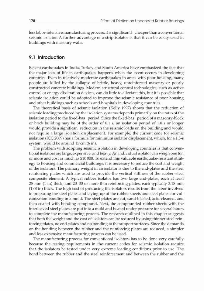
P1: TIX/XYZ P2: ABCJWST069-09 JWST069-Kelly-Style2 July 27, 2011 0:51 Printer Name: Yet to Come
178 Effect of Friction on Unbonded Rubber Bearings
less labor-intensive manufacturing process, it is significantl cheaper than a conventionalseismic isolator. A further advantage of a strip isolator is that it can be easily used inbuildings with masonry walls.
9.1 Introduction
Recent earthquakes in India, Turkey and South America have emphasized the fact thatthe major loss of life in earthquakes happens when the event occurs in developingcountries. Even in relatively moderate earthquakes in areas with poor housing, manypeople are killed by the collapse of brittle, heavy, unreinforced masonry or poorlyconstructed concrete buildings. Modern structural control technologies, such as activecontrol or energy dissipation devices, can do little to alleviate this, but it is possible thatseismic isolation could be adopted to improve the seismic resistance of poor housingand other buildings such as schools and hospitals in developing countries.
The theoretical basis of seismic isolation (Kelly 1997) shows that the reduction ofseismic loading produced by the isolation systems depends primarily on the ratio of theisolation period to the fixed-bas period. Since the fixed-bas period of a masonry-blockor brick building may be of the order of 0.1 s, an isolation period of 1.0 s or longerwould provide a significan reduction in the seismic loads on the building and wouldnot require a large isolation displacement. For example, the current code for seismicisolation (ICC 2009) has a formula for minimum isolator displacement, which, for a 1.5-ssystem, would be around 15 cm (6 in).
The problem with adopting seismic isolation in developing countries is that conven-tional isolators are large, expensive, and heavy. An individual isolator can weigh one tonor more and cost as much as $10 000. To extend this valuable earthquake-resistant strat-egy to housing and commercial buildings, it is necessary to reduce the cost and weightof the isolators. The primary weight in an isolator is due to the end-plates and the steelreinforcing plates which are used to provide the vertical stiffness of the rubber–steelcomposite element. A typical rubber isolator has two large end-plates, each at least25 mm (1 in) thick, and 20–30 or more thin reinforcing plates, each typically 3.18 mm(1/8 in) thick. The high cost of producing the isolators results from the labor involvedin preparing the steel plates and laying-up of the rubber sheets and steel plates for vul-canization bonding in a mold. The steel plates are cut, sand-blasted, acid-cleaned, andthen coated with bonding compound. Next, the compounded rubber sheets with theinterleaved steel plates are put into a mold and heated under pressure for several hoursto complete the manufacturing process. The research outlined in this chapter suggeststhat both the weight and the cost of isolators can be reduced by using thinner steel rein-forcing plates, no end-plates and no bonding to the support surfaces. Since the demandson the bonding between the rubber and the reinforcing plates are reduced, a simplerand less expensive manufacturing process can be used.
The manufacturing process for conventional isolators has to be done very carefullybecause the testing requirements in the current codes for seismic isolation requirethat the isolators be tested under very extreme loading conditions prior to use. Thebond between the rubber and the steel reinforcement and between the rubber and the
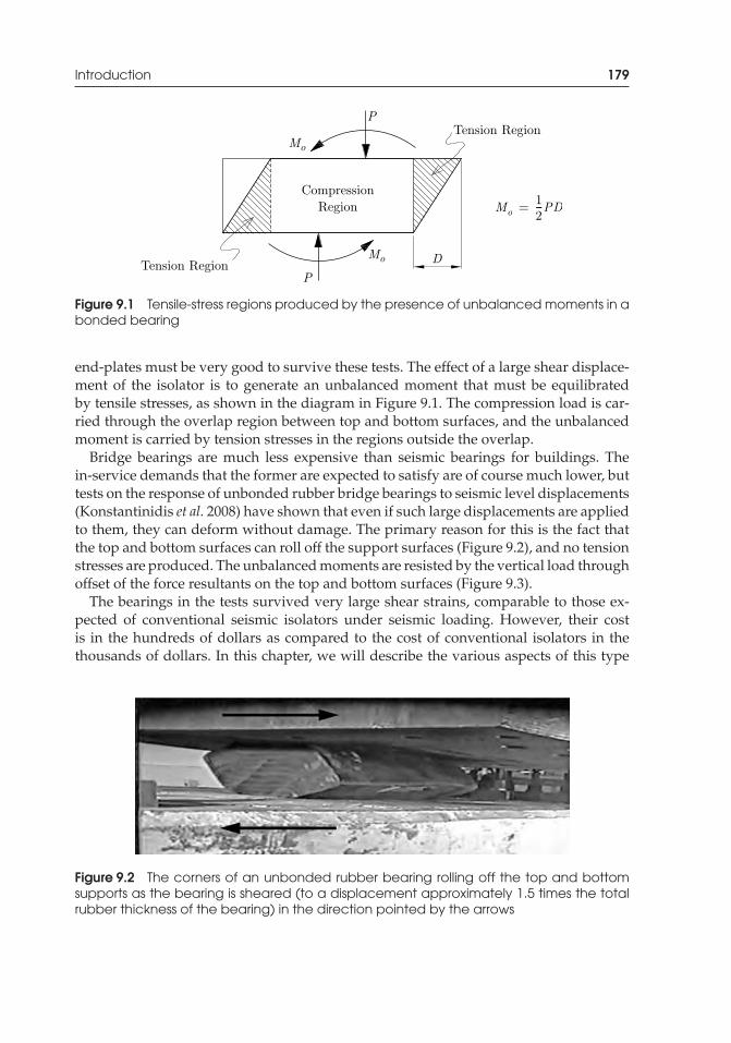
P1: TIX/XYZ P2: ABCJWST069-09 JWST069-Kelly-Style2 July 27, 2011 0:51 Printer Name: Yet to Come
Introduction 179
Figure 9.1 Tensile-stress regions produced by the presence of unbalanced moments in abonded bearing
end-plates must be very good to survive these tests. The effect of a large shear displace-ment of the isolator is to generate an unbalanced moment that must be equilibratedby tensile stresses, as shown in the diagram in Figure 9.1. The compression load is car-ried through the overlap region between top and bottom surfaces, and the unbalancedmoment is carried by tension stresses in the regions outside the overlap.
Bridge bearings are much less expensive than seismic bearings for buildings. Thein-service demands that the former are expected to satisfy are of course much lower, buttests on the response of unbonded rubber bridge bearings to seismic level displacements(Konstantinidis et al. 2008) have shown that even if such large displacements are appliedto them, they can deform without damage. The primary reason for this is the fact thatthe top and bottom surfaces can roll off the support surfaces (Figure 9.2), and no tensionstresses are produced. The unbalanced moments are resisted by the vertical load throughoffset of the force resultants on the top and bottom surfaces (Figure 9.3).
The bearings in the tests survived very large shear strains, comparable to those ex-pected of conventional seismic isolators under seismic loading. However, their costis in the hundreds of dollars as compared to the cost of conventional isolators in thethousands of dollars. In this chapter, we will describe the various aspects of this type
Figure 9.2 The corners of an unbonded rubber bearing rolling off the top and bottomsupports as the bearing is sheared (to a displacement approximately 1.5 times the totalrubber thickness of the bearing) in the direction pointed by the arrows
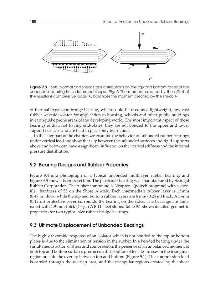
P1: TIX/XYZ P2: ABCJWST069-09 JWST069-Kelly-Style2 July 27, 2011 0:51 Printer Name: Yet to Come
180 Effect of Friction on Unbonded Rubber Bearings
Figure 9.3 Left: Normal and shear stress distributions on the top and bottom faces of theunbonded bearing in its deformed shape. Right: The moment created by the offset ofthe resultant compressive loads, P, balances the moment created by the shear, V
of thermal expansion bridge bearing, which could be used as a lightweight, low-costrubber seismic isolator for application to housing, schools and other public buildingsin earthquake prone areas of the developing world. The most important aspect of thesebearings is that, not having end-plates, they are not bonded to the upper and lowersupport surfaces and are held in place only by friction.
In the later part of the chapter, we examine the behavior of unbonded rubber bearingsunder vertical load and show that slip between the unbonded surfaces and rigid supportsabove and below can have a significan influenc on the vertical stiffness and the internalpressure distribution.
9.2 Bearing Designs and Rubber Properties
Figure 9.4 is a photograph of a typical unbonded multilayer rubber bearing, andFigure 9.5 shows its cross-section. The particular bearing was manufactured by ScougalRubber Corporation. The rubber compound is Neoprene (polychloroprene) with a spec-ifie hardness of 55 on the Shore A scale. Each intermediate rubber layer is 12 mm(0.47 in) thick, while the top and bottom rubber layers are 6 mm (0.24 in) thick. A 3-mm(0.12 in) protective cover surrounds the bearing on the sides. The bearings are lami-nated with 1.9-mm-thick (14-ga) A1011 steel shims. Table 9.1 shows detailed geometricproperties for two typical-size rubber bridge bearings.
9.3 Ultimate Displacement of Unbonded Bearings
The highly favorable response of an isolator which is not bonded to the top or bottomplates is due to the elimination of tension in the rubber. In a bonded bearing under thesimultaneous action of shear and compression, the presence of an unbalanced moment atboth top and bottom surfaces produces a distribution of tensile stresses in the triangularregion outside the overlap between top and bottom (Figure 9.1). The compression loadis carried through the overlap area, and the triangular regions created by the shear
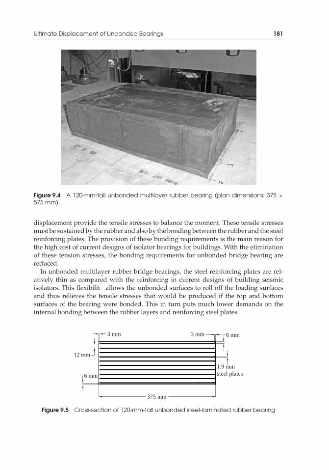
P1: TIX/XYZ P2: ABCJWST069-09 JWST069-Kelly-Style2 July 27, 2011 0:51 Printer Name: Yet to Come
Ultimate Displacement of Unbonded Bearings 181
Figure 9.4 A 120-mm-tall unbonded multilayer rubber bearing (plan dimensions: 375 ×575 mm).
displacement provide the tensile stresses to balance the moment. These tensile stressesmust be sustained by the rubber and also by the bonding between the rubber and the steelreinforcing plates. The provision of these bonding requirements is the main reason forthe high cost of current designs of isolator bearings for buildings. With the eliminationof these tension stresses, the bonding requirements for unbonded bridge bearing arereduced.
In unbonded multilayer rubber bridge bearings, the steel reinforcing plates are rel-atively thin as compared with the reinforcing in current designs of building seismicisolators. This flexibilit allows the unbonded surfaces to roll off the loading surfacesand thus relieves the tensile stresses that would be produced if the top and bottomsurfaces of the bearing were bonded. This in turn puts much lower demands on theinternal bonding between the rubber layers and reinforcing steel plates.
3 mm
6 mm
12 mm
3 mm
375 mm
6 mm
1.9 mmsteel plates
Figure 9.5 Cross-section of 120-mm-tall unbonded steel-laminated rubber bearing
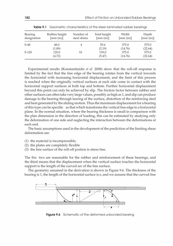
P1: TIX/XYZ P2: ABCJWST069-09 JWST069-Kelly-Style2 July 27, 2011 0:51 Printer Name: Yet to Come
182 Effect of Friction on Unbonded Rubber Bearings
Table 9.1 Geometric characteristics of the steel–laminated rubber bearings
Bearing Rubber height Number of Total height Width Depthdesignation [mm (in)] steel shims [mm (in)] [mm (in)] [mm (in)]
S-48 48.0(1.89)
4 55.6(2.19)
375.0(14.76)
575.0(22.64)
S-120 120.0(4.72)
10 139.0(5.47)
375.0(14.76)
575.0(22.64)
Experimental results (Konstantinidis et al. 2008) show that the roll-off response islimited by the fact that the free edge of the bearing rotates from the vertical towardsthe horizontal with increasing horizontal displacement, and the limit of this processis reached when the originally vertical surfaces at each side come in contact with thehorizontal support surfaces at both top and bottom. Further horizontal displacementbeyond this point can only be achieved by slip. The friction factor between rubber andother surfaces can often take very large values, possibly as high as 1, and slip can producedamage to the bearing through tearing of the surface, distortion of the reinforcing steeland heat generated by the sliding motion. Thus the maximum displacement for a bearingof this type can be specifie as that which transforms the vertical free edge to a horizontalplane. In the normal situation, where the bearing thickness is small in comparison withthe plan dimension in the direction of loading, this can be estimated by studying onlythe deformation of one side and neglecting the interaction between the deformations ateach end.
The basic assumptions used in the development of the prediction of the limiting sheardeformation are:
(1) the material is incompressible;(2) the plates are completely flexible(3) the free surface of the roll-off portion is stress free.
The firs two are reasonable for the rubber and reinforcement of these bearings, andthe third means that the displacement when the vertical surface touches the horizontalsupport is the length of the curved arc of the free surface.
The geometry assumed in the derivation is shown in Figure 9.6. The thickness of thebearing is 1, the length of the horizontal surface is a, and we assume that the curved free
Figure 9.6 Schematic of the deformed unbonded bearing

P1: TIX/XYZ P2: ABCJWST069-09 JWST069-Kelly-Style2 July 27, 2011 0:51 Printer Name: Yet to Come
Ultimate Displacement of Unbonded Bearings 183
surface is a parabolic arc; then in the coordinate system (x, y) shown in Figure 9.6, thecurved surface is given by
y = x2
a 2 , or x = a√y (9.1)
The area of the region enclosed by the curved arc of length S is
A=1∫
0
dy
a√y∫
0
dx = 23a (9.2)
The requirement of incompressibility means that the volume before deformation andafter are preserved. Thus,
12S = 2
3a or a = 3
4S (9.3)
The curved arc length S is given by
dS =√
dx2 + dy2 (9.4)
where
dy = 2xa 2 dx (9.5)
and
S =a∫
0
√1 + 4x2
a 4 dx (9.6)
Using the change of variable u = 2x/a 2, we have
S = a2
2
2/a∫0
√1 + u2du (9.7)
Letting u = sinh t, we have
S = a2
2
sinh−1(2/a )∫0
cosh2 tdt (9.8)
Since cosh2 t = (cosh(2t) + 1)/2, this leads to
S = a2
4[sinh t cosh t + t]sinh−1(2/a )
0 (9.9)
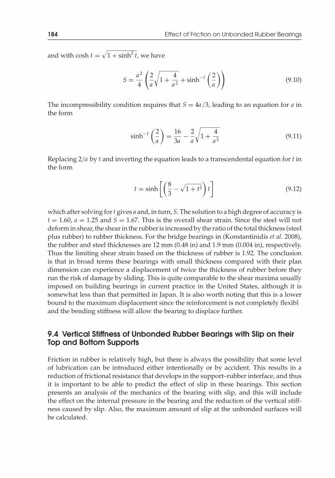
P1: TIX/XYZ P2: ABCJWST069-09 JWST069-Kelly-Style2 July 27, 2011 0:51 Printer Name: Yet to Come
184 Effect of Friction on Unbonded Rubber Bearings
and with cosh t =√
1 + sinh2 t, we have
S = a2
4
(2a
√1 + 4
a2 + sinh−1(
2a
))(9.10)
The incompressibility condition requires that S = 4a/3, leading to an equation for a inthe form
sinh−1(
2a
)= 16
3a− 2a
√1 + 4
a2 (9.11)
Replacing 2/a by t and inverting the equation leads to a transcendental equation for t inthe form
t = sinh[(
83
−√
1 + t2)t]
(9.12)
which after solving for tgives a and, in turn,S. The solution to a high degree of accuracy ist = 1.60, a = 1.25 and S = 1.67. This is the overall shear strain. Since the steel will notdeform in shear, the shear in the rubber is increased by the ratio of the total thickness (steelplus rubber) to rubber thickness. For the bridge bearings in (Konstantinidis et al. 2008),the rubber and steel thicknesses are 12 mm (0.48 in) and 1.9 mm (0.004 in), respectively.Thus the limiting shear strain based on the thickness of rubber is 1.92. The conclusionis that in broad terms these bearings with small thickness compared with their plandimension can experience a displacement of twice the thickness of rubber before theyrun the risk of damage by sliding. This is quite comparable to the shear maxima usuallyimposed on building bearings in current practice in the United States, although it issomewhat less than that permitted in Japan. It is also worth noting that this is a lowerbound to the maximum displacement since the reinforcement is not completely flexibland the bending stiffness will allow the bearing to displace further.
9.4 Vertical Stiffness of Unbonded Rubber Bearings with Slip on theirTop and Bottom Supports
Friction in rubber is relatively high, but there is always the possibility that some levelof lubrication can be introduced either intentionally or by accident. This results in areduction of frictional resistance that develops in the support–rubber interface, and thusit is important to be able to predict the effect of slip in these bearings. This sectionpresents an analysis of the mechanics of the bearing with slip, and this will includethe effect on the internal pressure in the bearing and the reduction of the vertical stiff-ness caused by slip. Also, the maximum amount of slip at the unbonded surfaces willbe calculated.
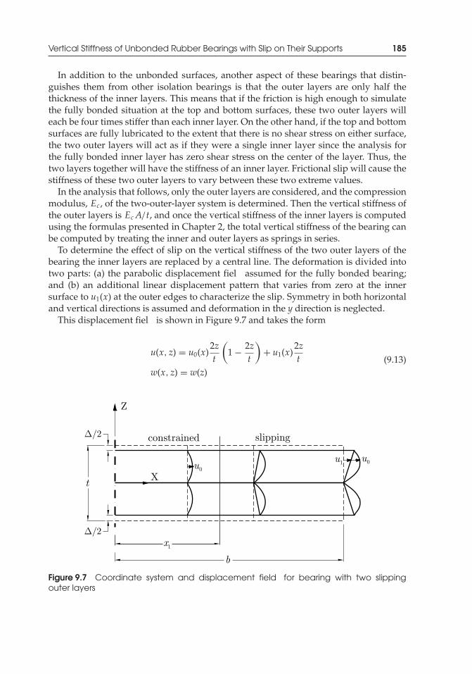
P1: TIX/XYZ P2: ABCJWST069-09 JWST069-Kelly-Style2 July 27, 2011 0:51 Printer Name: Yet to Come
Vertical Stiffness of Unbonded Rubber Bearings with Slip on Their Supports 185
In addition to the unbonded surfaces, another aspect of these bearings that distin-guishes them from other isolation bearings is that the outer layers are only half thethickness of the inner layers. This means that if the friction is high enough to simulatethe fully bonded situation at the top and bottom surfaces, these two outer layers willeach be four times stiffer than each inner layer. On the other hand, if the top and bottomsurfaces are fully lubricated to the extent that there is no shear stress on either surface,the two outer layers will act as if they were a single inner layer since the analysis forthe fully bonded inner layer has zero shear stress on the center of the layer. Thus, thetwo layers together will have the stiffness of an inner layer. Frictional slip will cause thestiffness of these two outer layers to vary between these two extreme values.
In the analysis that follows, only the outer layers are considered, and the compressionmodulus, Ec , of the two-outer-layer system is determined. Then the vertical stiffness ofthe outer layers is Ec A/t, and once the vertical stiffness of the inner layers is computedusing the formulas presented in Chapter 2, the total vertical stiffness of the bearing canbe computed by treating the inner and outer layers as springs in series.
To determine the effect of slip on the vertical stiffness of the two outer layers of thebearing the inner layers are replaced by a central line. The deformation is divided intotwo parts: (a) the parabolic displacement fiel assumed for the fully bonded bearing;and (b) an additional linear displacement pattern that varies from zero at the innersurface to u1(x) at the outer edges to characterize the slip. Symmetry in both horizontaland vertical directions is assumed and deformation in the y direction is neglected.
This displacement fiel is shown in Figure 9.7 and takes the form
u(x, z) = u0(x)2zt
(1 − 2z
t
)+ u1(x)
2zt
w(x, z) = w(z)(9.13)
Figure 9.7 Coordinate system and displacement field for bearing with two slippingouter layers
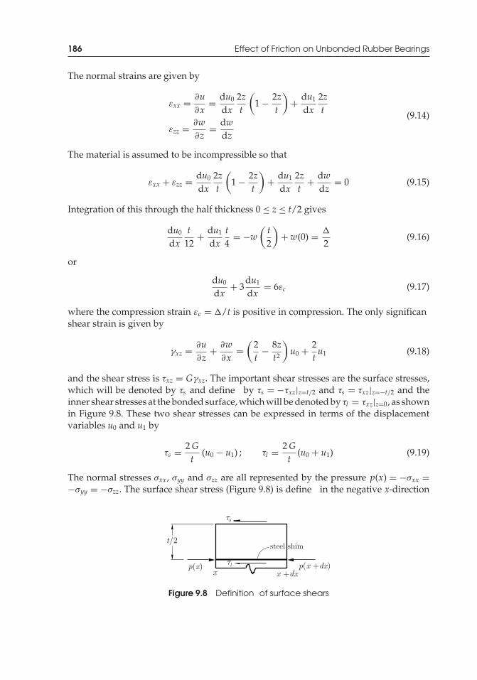
P1: TIX/XYZ P2: ABCJWST069-09 JWST069-Kelly-Style2 July 27, 2011 0:51 Printer Name: Yet to Come
186 Effect of Friction on Unbonded Rubber Bearings
The normal strains are given by
εxx = ∂u∂x
= du0
dx2zt
(1 − 2z
t
)+ du1
dx2zt
εzz = ∂w∂z
= dwdz
(9.14)
The material is assumed to be incompressible so that
εxx + εzz = du0
dx2zt
(1 − 2z
t
)+ du1
dx2zt
+ dwdz
= 0 (9.15)
Integration of this through the half thickness 0 ≤ z ≤ t/2 gives
du0
dxt
12+ du1
dxt4
= −w(t2
)+ w(0) = �
2(9.16)
or
du0
dx+ 3
du1
dx= 6εc (9.17)
where the compression strain εc = �/t is positive in compression. The only significanshear strain is given by
γxz = ∂u∂z
+ ∂w∂x
=(
2t
− 8zt2
)u0 + 2
tu1 (9.18)
and the shear stress is τxz = Gγxz. The important shear stresses are the surface stresses,which will be denoted by τs and define by τs = −τxz|z=t/2 and τs = τxz|z=−t/2 and theinner shear stresses at the bonded surface, which will be denoted by τl = τxz|z=0, as shownin Figure 9.8. These two shear stresses can be expressed in terms of the displacementvariables u0 and u1 by
τs = 2Gt
(u0 − u1) ; τl = 2Gt
(u0 + u1) (9.19)
The normal stresses σxx, σyy and σzz are all represented by the pressure p(x) = −σxx =−σyy = −σzz. The surface shear stress (Figure 9.8) is define in the negative x-direction
t/2
s
l
steel shim
p(x +dx)p(x)x x +dx
Figure 9.8 Definition of surface shears
P1: TIX/XYZ P2: ABCJWST069-09 JWST069-Kelly-Style2 July 27, 2011 0:51 Printer Name: Yet to Come
Vertical Stiffness of Unbonded Rubber Bearings with Slip on Their Supports 187
on the top surface and in the positive direction on the bottom surface, as shown in thediagram, to allow us to make use of symmetry.
The assumption that all the normal stress components are equal to the negative pres-sure reduces the equations of stress equilibrium to the single equation
∂τxz
∂z= dp
dx(9.20)
and integration of this through the upper half layer 0 ≤ z ≤ t/2 gives
t/2∫0
∂τxz
∂zdz = t
2dpdx
= −(τs + τl) (9.21)
which is also shown in the diagram. From this equation and the fact that for both the non-slip and slipped regions, τs + τl = 4Gu0/t, we have a connection between the pressureand the displacement fiel valid everywhere in the form
dpdx
= −8Gt2 u0 (9.22)
We assume that slip occurs at x = x1 and assume symmetry and continuity at x = 0 andx = x1. In the non-slip region 0 ≤ x ≤ x1, we have u1 = 0, and with the above equation,we have
u0 = − t2
8Gdpdx
(9.23)
Substitution into the equation of incompressibility, which now takes the formdu0/dx = 6εc , gives
d2 pdx2 = −48Gεc
t2 (9.24)
from which
p(x) = −24Gεc
t2 x2 + Ax + B
Symmetry dictates that A = 0, and, if there were no slip, we could use a boundarycondition at x= b to determine B. In this case, we cannot use such a condition and mustleave B as an unknown. It is convenient to absorb it into the other constants and writep(x) and dp/dx as
p(x) = 24GS2εc
(B − x2
b2
), 0 ≤ x ≤ x1 (9.25)
dpdx
= −48Gεc
t2 x, 0 ≤ x ≤ x1 (9.26)
P1: TIX/XYZ P2: ABCJWST069-09 JWST069-Kelly-Style2 July 27, 2011 0:51 Printer Name: Yet to Come
188 Effect of Friction on Unbonded Rubber Bearings
The displacement fiel in this region is simply u0 = 6xεc and u1 = 0. We note that atx = x1 the value of the surface shear stress is related to the pressure through τs = μp,where μ is the coefficien of friction, so that from Equations (9.17) and (9.22)
48Gεc
tx1 = 24μGεc
b2
t2
(B − x2
1
b2
)
or
x1 = μb2
2t
(B − x2
1
b2
)(9.27)
which shows that the location of the slip is not affected by the level of the compressionstrain.
For the region x1 ≤ x ≤ b, where u1 �= 0, the equation of incompressibility becomes
du0
dx+ 3
du1
dx= 6εc (9.28)
This can be integrated over the region x1 ≤ x ≤ b using the fact that continuity requiresthat u0(x1) = 6x1εc and u1(x1) = 0, giving
u0(x) + 3u1(x) = 6xεc (9.29)
In addition, over the slipped region, we have τs = μp and also dp/dx = −2(τs + τl )/t,which taken together give
dpdx
+ 2μ
tp = −2
tτl = −4G
t2 (u0 + u1) (9.30)
We can replace u1 using the integrated form of the equation of incompressibility,leading to
dpdx
+ 2μ
tp = −4G
t2
(23u0 + 2xεc
)(9.31)
which, in turn, by replacing u0 from Equation (9.22), gives
dpdx
+ 3μ
tp = −12Gεc
t2 x (9.32)
Using the integrating factor e3μx/t, this can be written in the form
ddx
(e3μx/t p) = −12Gεc
t2xe3μx/t (9.33)
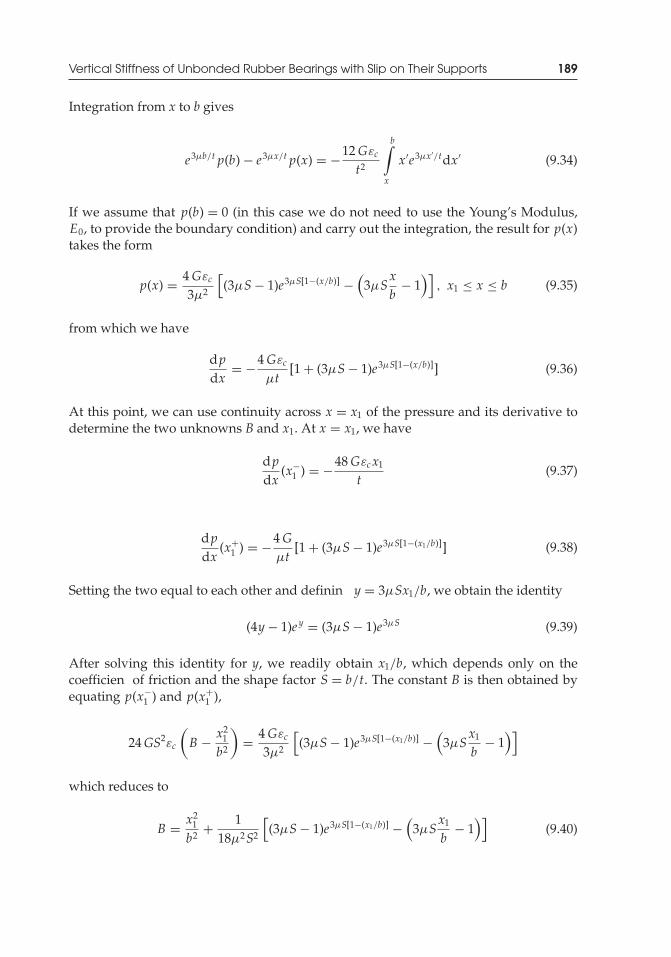
P1: TIX/XYZ P2: ABCJWST069-09 JWST069-Kelly-Style2 July 27, 2011 0:51 Printer Name: Yet to Come
Vertical Stiffness of Unbonded Rubber Bearings with Slip on Their Supports 189
Integration from x to b gives
e3μb/t p(b) − e3μx/t p(x) = −12Gεc
t2
b∫x
x′e3μx′/tdx′ (9.34)
If we assume that p(b) = 0 (in this case we do not need to use the Young’s Modulus,E0, to provide the boundary condition) and carry out the integration, the result for p(x)takes the form
p(x) = 4Gεc
3μ2
[(3μS− 1)e3μS[1−(x/b)] −
(3μS
xb
− 1)]
, x1 ≤ x ≤ b (9.35)
from which we have
dpdx
= −4Gεc
μt[1 + (3μS− 1)e3μS[1−(x/b)]] (9.36)
At this point, we can use continuity across x = x1 of the pressure and its derivative todetermine the two unknowns B and x1. At x = x1, we have
dpdx
(x−1 ) = −48Gεcx1
t(9.37)
dpdx
(x+1 ) = −4G
μt[1 + (3μS− 1)e3μS[1−(x1/b)]] (9.38)
Setting the two equal to each other and definin y = 3μSx1/b, we obtain the identity
(4y− 1)e y = (3μS− 1)e3μS (9.39)
After solving this identity for y, we readily obtain x1/b, which depends only on thecoefficien of friction and the shape factor S = b/t. The constant B is then obtained byequating p(x−
1 ) and p(x+1 ),
24GS2εc
(B − x2
1
b2
)= 4Gεc
3μ2
[(3μS− 1)e3μS[1−(x1/b)] −
(3μS
x1
b− 1
)]
which reduces to
B = x21
b2 + 118μ2S2
[(3μS− 1)e3μS[1−(x1/b)] −
(3μS
x1
b− 1
)](9.40)
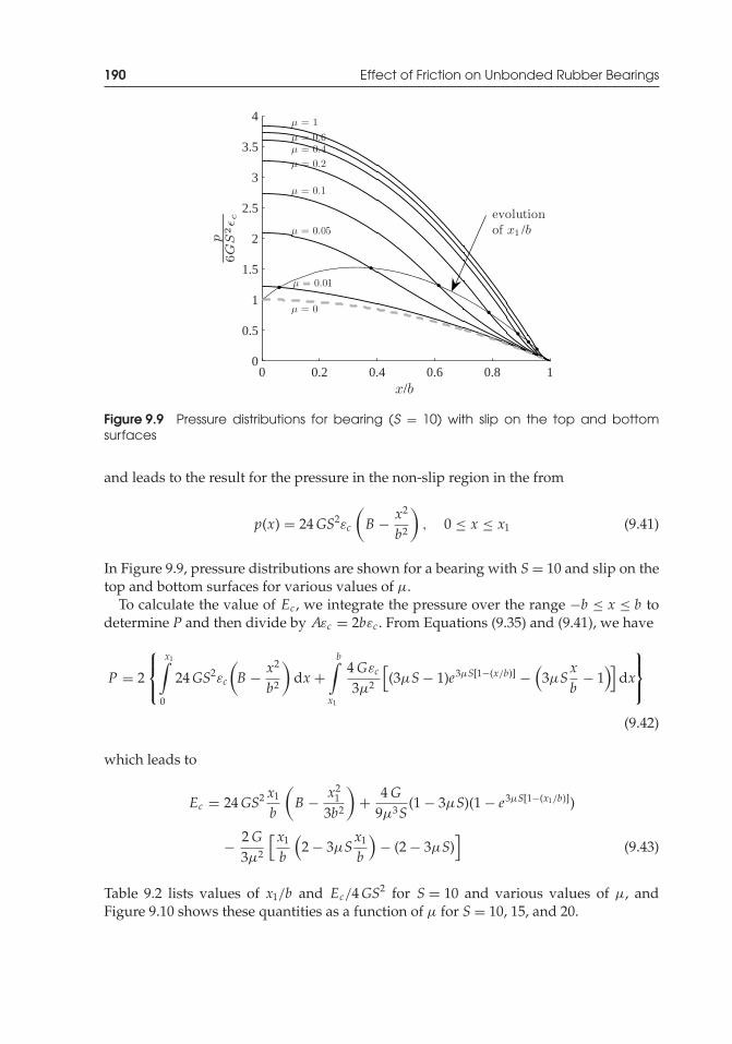
P1: TIX/XYZ P2: ABCJWST069-09 JWST069-Kelly-Style2 July 27, 2011 0:51 Printer Name: Yet to Come
190 Effect of Friction on Unbonded Rubber Bearings
0 0.2 0.4 0.6 0.8 10
0.5
1
1.5
2
2.5
3
3.5
4
x/b
p6GS
2εc
µ = 0.01
µ = 0.05
µ = 0.1
µ = 0.2µ = 0.4µ = 0.6µ = 1
µ = 0
evolutionof x /b1
Figure 9.9 Pressure distributions for bearing (S = 10) with slip on the top and bottomsurfaces
and leads to the result for the pressure in the non-slip region in the from
p(x) = 24GS2εc
(B − x2
b2
), 0 ≤ x ≤ x1 (9.41)
In Figure 9.9, pressure distributions are shown for a bearing with S = 10 and slip on thetop and bottom surfaces for various values of μ.
To calculate the value of Ec , we integrate the pressure over the range −b ≤ x ≤ b todetermine P and then divide by Aεc = 2bεc . From Equations (9.35) and (9.41), we have
P = 2
⎧⎨⎩
x1∫0
24GS2εc
(B − x2
b2
)dx +
b∫x1
4Gεc
3μ2
[(3μS− 1)e3μS[1−(x/b)] −
(3μS
xb
− 1)]
dx
⎫⎬⎭
(9.42)
which leads to
Ec = 24GS2 x1
b
(B − x2
1
3b2
)+ 4G
9μ3S(1 − 3μS)(1 − e3μS[1−(x1/b)])
− 2G3μ2
[x1
b
(2 − 3μS
x1
b
)− (2 − 3μS)
](9.43)
Table 9.2 lists values of x1/b and Ec/4GS2 for S = 10 and various values of μ, andFigure 9.10 shows these quantities as a function of μ for S = 10, 15, and 20.
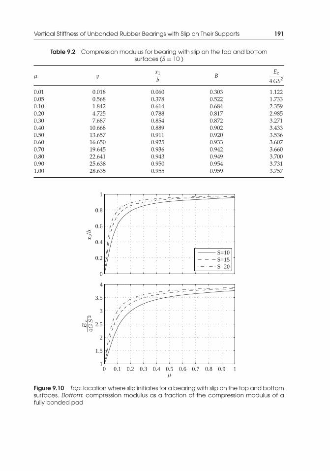
P1: TIX/XYZ P2: ABCJWST069-09 JWST069-Kelly-Style2 July 27, 2011 0:51 Printer Name: Yet to Come
Vertical Stiffness of Unbonded Rubber Bearings with Slip on Their Supports 191
Table 9.2 Compression modulus for bearing with slip on the top and bottomsurfaces (S = 10 )
μ yx1
bB
Ec
4GS2
0.01 0.018 0.060 0.303 1.1220.05 0.568 0.378 0.522 1.7330.10 1.842 0.614 0.684 2.3590.20 4.725 0.788 0.817 2.9850.30 7.687 0.854 0.872 3.2710.40 10.668 0.889 0.902 3.4330.50 13.657 0.911 0.920 3.5360.60 16.650 0.925 0.933 3.6070.70 19.645 0.936 0.942 3.6600.80 22.641 0.943 0.949 3.7000.90 25.638 0.950 0.954 3.7311.00 28.635 0.955 0.959 3.757
0
0.2
0.4
0.6
0.8
1
x /b
1
0 0.1 0.2 0.3 0.4 0.5 0.6 0.7 0.8 0.9 11
1.5
2
2.5
3
3.5
4
Ec
4GS
2
µ
S=10S=15S=20
Figure 9.10 Top: location where slip initiates for a bearing with slip on the top and bottomsurfaces. Bottom: compression modulus as a fraction of the compression modulus of afully bonded pad
P1: TIX/XYZ P2: ABCJWST069-09 JWST069-Kelly-Style2 July 27, 2011 0:51 Printer Name: Yet to Come
192 Effect of Friction on Unbonded Rubber Bearings
This chapter has provided an analysis of a type of rubber bearing that is not bondedto the supports above and below it, but held in place solely by friction. These bearingshave been previously tested and survived very large shear strains (of the order of200% or larger, Konstantinidis et al. 2008). While the seismic performance objectivesthat unbonded bearings are expected to achieve are not as high as those of isolationbearings, their low cost and light weight makes them very appealing for use as a low-cost alternative to seismic isolators for schools, housing and other public buildings inhighly seismic areas of the developing world, where conventional seismic isolators arenot affordable (Kelly and Konstantinidis 2007).
The effect of the frictional resistance of the top and bottom supports on the pressuredistribution and the compression modulus of an unbonded bearing under compressiveload were firs examined by Kelly and Konstantinidis (2009b) in an effort to predict thebehavior of a type of rubber bridge bearing permitted in California for use as a thermalexpansion bridge bearing. The analysis shows that friction has an important effect onboth the maximum pressure and the compression modulus.

P1: TIX/XYZ P2: ABCJWST069-APP JWST069-Kelly-Style2 July 12, 2011 9:4 Printer Name: Yet to Come
AppendixElastic Connection Devicefor One or More Degreesof FreedomMr Eugene Freyssinet, resident in France (Seine)
Mechanics of Rubber Bearings for Seismic and Vibration Isolation, First Edition. James M. Kelly and Dimitrios A. Konstantinidis.C© 2011 John Wiley & Sons, Ltd. Published 2011 by John Wiley & Sons, Ltd.
193

P1: TIX/XYZ P2: ABCJWST069-APP JWST069-Kelly-Style2 July 12, 2011 9:4 Printer Name: Yet to Come
194 Appendix: Elastic Connection Device for One or More Degrees of Freedom
P1: TIX/XYZ P2: ABCJWST069-APP JWST069-Kelly-Style2 July 12, 2011 9:4 Printer Name: Yet to Come
Appendix: Elastic Connection Device for One or More Degrees of Freedom 195
P1: TIX/XYZ P2: ABCJWST069-APP JWST069-Kelly-Style2 July 12, 2011 9:4 Printer Name: Yet to Come
196 Appendix: Elastic Connection Device for One or More Degrees of Freedom
P1: TIX/XYZ P2: ABCJWST069-APP JWST069-Kelly-Style2 July 12, 2011 9:4 Printer Name: Yet to Come
Appendix: Elastic Connection Device for One or More Degrees of Freedom 197
P1: TIX/XYZ P2: ABCJWST069-APP JWST069-Kelly-Style2 July 12, 2011 9:4 Printer Name: Yet to Come
198 Appendix: Elastic Connection Device for One or More Degrees of Freedom
P1: TIX/XYZ P2: ABCJWST069-APP JWST069-Kelly-Style2 July 12, 2011 9:4 Printer Name: Yet to Come
Appendix: Elastic Connection Device for One or More Degrees of Freedom 199
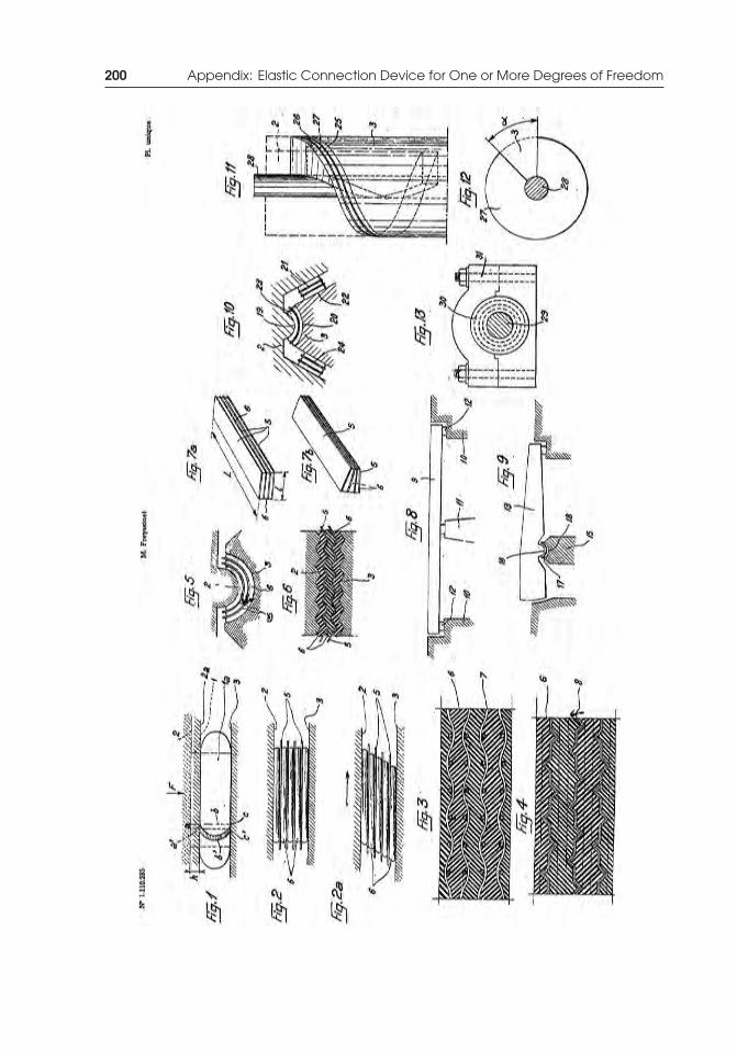
P1: TIX/XYZ P2: ABCJWST069-APP JWST069-Kelly-Style2 July 12, 2011 9:4 Printer Name: Yet to Come
200 Appendix: Elastic Connection Device for One or More Degrees of Freedom
P1: TIX/XYZ P2: ABCJWST069-APP JWST069-Kelly-Style2 July 12, 2011 9:4 Printer Name: Yet to Come
Appendix: Elastic Connection Device for One or More Degrees of Freedom 201
Application on 25 May 1954, 16h 47m, in ParisIssued on 12 October 1955.—Published 10 February 1956
(Patent of invention, the grant has been issued pursuant to Article 11, § 7, of the Law of 5 July1844 amended by the Act of 7 April 1902.)
Mechanical construction projects frequently require connections between rigid parts thatallow relative displacements, with one or more degrees of freedom, between these parts.One can provide these by means of machined mechanical components, eliminating bylubrication the friction between bearing surfaces or by intermediate roller bearings,providing connections with a limited number of degrees of freedom. Obtaining severaldegrees of freedom at a time can often require very complex assemblies. The connectionsthat use machined components are nevertheless regarded as essential when the struc-tures are important or when a high degree of accuracy is required in providing relativedisplacements between the parts.
However, it has already been proposed that in the case of relatively low forces andalso when the precision in the displacement is not required, that connections allowinglimited displacements can be provided, by interposing rubber-like components betweenthe rigid parts. These rubber parts working through the distortion of the rubber, allowrelative movements with low friction and provide the added advantage of an elasticrecovery after displacement from their original position. This type of connection hasanother advantage in the fact that they need no maintenance and are protected from thetype of seizure to which links made with mechanical parts are subject.
The purpose of the present invention is the realization of connections between rigidparts that allow displacements on boundaries with at least one degree of freedom by theuse of rubber components that are deformed by distortion, but, unlike the conventionalconnections using rubber, these connections can have virtually unlimited size and canensure precise radial relative displacements to parts as large as we desire.
It thus becomes possible to apply such connections in projects involving huge efforts,as is the case in public works or in high-precision machines with very small dimensionaltolerances. Nevertheless, the invention allows these results to be achieved with coststhat are very economic both in terms of the raw materials used and for labor costsand machining.
According to the invention, a block formed of rubber plates within which are inter-spersed inextensible sheets whose surfaces are parallel to the surfaces of the rigid partsand which have a large coefficien of friction in contact with the rubber plates, is inter-posed between the substantially parallel surfaces of two rigid parts to which one wishesto establish a connection.
The high coefficien of friction can be obtained by bonding between the inextensiblesheets and the plates of rubber or, preferably, by using an inextensible sheet surface witha strong surface roughness such as embossed, perforated or corrugated sheets or yetagain gratings.
Preferably, the block formed by the assembly of the alternating plates of rubber andinextensible sheets is compressed in the direction perpendicular to the surfaces of thesheets, either by a prior compression or by the loads applied to the rigid parts includingthe weight of these parts.
P1: TIX/XYZ P2: ABCJWST069-APP JWST069-Kelly-Style2 July 12, 2011 9:4 Printer Name: Yet to Come
202 Appendix: Elastic Connection Device for One or More Degrees of Freedom
It will be shown later in the memoir that the deformation that can be sustained bysuch a block under the applied compression depends only to a small degree on theelasticity modulus of the rubber, and that it is possible to apply to such a block loads,within the extent of crushing of the rubber, that, nevertheless, allows in directionstangential to the lamination, displacements between the two rigid parts by distortionof the rubber that separates them, in the same way as would happen if this rubber wasnot laminated by the sheets.
The displacements permitted by such a laminated block, interposed between parallelsurfaces, correspond mainly to the possibility of two parallel surfaces to slide one versusthe other while remaining in contact over all of their extent.
Geometrically, the surfaces that perfectly satisfy this condition are the plane, thesurfaces of revolution (including the sphere) and the helicoidal surfaces. Nevertheless,should the movements be limited, other surfaces of more complex geometric definitiocan be chosen for the surfaces of the rigid parts, if the approximation of parallelismcorresponding to the maximum displacement remains acceptable.
With surfaces that meet the strict requirement of parallelism during the relative dis-placement, it is possible to obtain the following displacements:
Two parallel fla surfaces allow for translations in all directions in their plane and alsorotations around any axis perpendicular to their plane;
Two parallel surfaces of revolution can rotate around their common axis and possiblya translation along this axis if these surfaces are cylinders or portions of a cylinder;in the case of two spheres, the axis of relative rotation is any axis provided it passesthrough the common center of these two spheres;
Two helicoidal surfaces permit a helical displacement, i.e., the combination of a trans-lation and a rotation.
It was implicitly assumed in the above that the distribution of stresses in the laminatedblock remained the same during the motion and, therefore, this block is distorted bythe deformation of the rubber. One can however also vary the distribution of stressesin the laminated block during the displacement by means of elastic deformation, thusproviding additional degrees of freedom. Thus, a prismatic block, laminated parallel toits bases, can allow not only translations parallel to these bases or rotations perpendicularto them, but also rotations with an axial component parallel to the plane of these bases, arotation which allows a dihedral angle between the planes of these bases. It may facilitatea displacement of this kind by giving to such a prismatic block a rectangular sectionaligned in the direction of the preferred axis of rotation.
One of the main applications of the invention is the realization of support pads forstructures that allow for displacements of these structures by internal causes (expan-sion) or by external causes (moving structures such as turning or lifting bridges, damgates, etc.).
For such works the invention allows the substitution for heavy metal componentswhich have machining and maintenance requirements by components that are easy toinstall, do not need extreme precision in their execution and installation and that willwork reliably, even in the absence of maintenance. In addition, the invention allows therealization of high-precision mechanical joints in machines and equipment, especially in
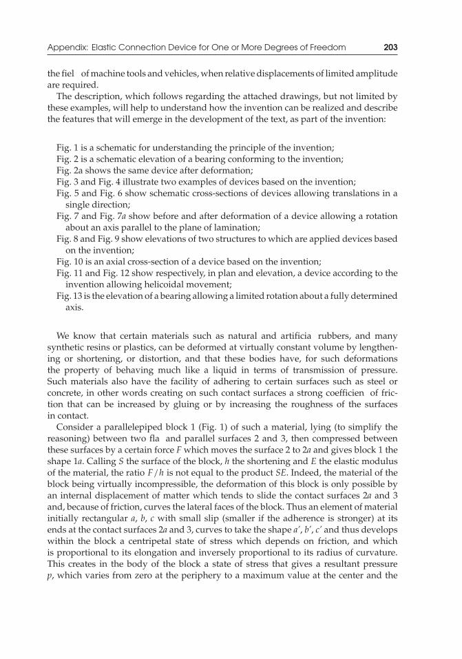
P1: TIX/XYZ P2: ABCJWST069-APP JWST069-Kelly-Style2 July 12, 2011 9:4 Printer Name: Yet to Come
Appendix: Elastic Connection Device for One or More Degrees of Freedom 203
the fiel of machine tools and vehicles, when relative displacements of limited amplitudeare required.
The description, which follows regarding the attached drawings, but not limited bythese examples, will help to understand how the invention can be realized and describethe features that will emerge in the development of the text, as part of the invention:
Fig. 1 is a schematic for understanding the principle of the invention;Fig. 2 is a schematic elevation of a bearing conforming to the invention;Fig. 2a shows the same device after deformation;Fig. 3 and Fig. 4 illustrate two examples of devices based on the invention;Fig. 5 and Fig. 6 show schematic cross-sections of devices allowing translations in a
single direction;Fig. 7 and Fig. 7a show before and after deformation of a device allowing a rotation
about an axis parallel to the plane of lamination;Fig. 8 and Fig. 9 show elevations of two structures to which are applied devices based
on the invention;Fig. 10 is an axial cross-section of a device based on the invention;Fig. 11 and Fig. 12 show respectively, in plan and elevation, a device according to the
invention allowing helicoidal movement;Fig. 13 is the elevation of a bearing allowing a limited rotation about a fully determined
axis.
We know that certain materials such as natural and artificia rubbers, and manysynthetic resins or plastics, can be deformed at virtually constant volume by lengthen-ing or shortening, or distortion, and that these bodies have, for such deformationsthe property of behaving much like a liquid in terms of transmission of pressure.Such materials also have the facility of adhering to certain surfaces such as steel orconcrete, in other words creating on such contact surfaces a strong coefficien of fric-tion that can be increased by gluing or by increasing the roughness of the surfacesin contact.
Consider a parallelepiped block 1 (Fig. 1) of such a material, lying (to simplify thereasoning) between two fla and parallel surfaces 2 and 3, then compressed betweenthese surfaces by a certain force F which moves the surface 2 to 2a and gives block 1 theshape 1a. Calling S the surface of the block, h the shortening and E the elastic modulusof the material, the ratio F/h is not equal to the product SE. Indeed, the material of theblock being virtually incompressible, the deformation of this block is only possible byan internal displacement of matter which tends to slide the contact surfaces 2a and 3and, because of friction, curves the lateral faces of the block. Thus an element of materialinitially rectangular a, b, c with small slip (smaller if the adherence is stronger) at itsends at the contact surfaces 2a and 3, curves to take the shape a’, b’, c’ and thus developswithin the block a centripetal state of stress which depends on friction, and whichis proportional to its elongation and inversely proportional to its radius of curvature.This creates in the body of the block a state of stress that gives a resultant pressurep, which varies from zero at the periphery to a maximum value at the center and the

P1: TIX/XYZ P2: ABCJWST069-APP JWST069-Kelly-Style2 July 12, 2011 9:4 Printer Name: Yet to Come
204 Appendix: Elastic Connection Device for One or More Degrees of Freedom
frictional stress on the surfaces a and c, caused by this pressure, also grow with this andreach their maximum value at the center of the block.
The resistance to the flattenin is not SE, but SE +� and if the smallest dimension inthe plane of the block is much larger than its thickness, the second term is much largerthan the firs providing the coefficien of friction of rubber on the surface of the rigidparts 2 and 3 is large.
If we assume that the thickness of the block 1 is halved, we see, assuming the samevalues of friction that the pressure p is doubled since the radius of curvature of elementof rubber is divided by two. Moreover, the value p, i.e., friction pϕ which before wasreached at a certain distance ρ from the periphery, is now reached at a distance ρ/2 fromthe same periphery. The pressure in the central zone will therefore be much larger and� will be much more than double.
If one considers, instead of a homogeneous rubber block 1, a block formed fromtwo plates of half thickness separated by a sheet of inextensible material with a highcoefficien of friction in contact with these plates, the presence of this sheet will have amultiplier effect of at least four in the resistance to deformation of this block comparedwith the homogeneous composite block.
The division of the block by nine intermediate sheets giving ten equal plates of rubbercan also increase the resistance by a factor of more than 100.
This resistance, unrelated to the intrinsic strength of the rubber against compression,can be increased without limit other than the resistance to efforts to stretch the interme-diate leaves and the lowering of the coefficien of friction with pressure, which reductionis only obtained under extremely high pressures.
One can create a block of rubber plates, as shown schematically in Fig. 2, separated by6 thin inextensible sheets 5 with a high coefficien of friction in contact with these plates.
If, as shown in Fig. 2a, there is a relative displacement between parts 2 and 3 in adirection parallel to the lamination, this displacement is produced by deformation overthe entire set of 6 plates providing there is adherence between the plates and sheets.
The force which opposes this displacement is always (SE .d)/e, where e is the totalthickness and d the amplitude of the displacement. It does not matter in fact that the totalthickness e is in one or several plates, since the division into plates also modifie equallyd and e. Moreover, in the case of a homogeneous block, the value of the force necessaryto cause the displacement is bounded in the block by the presence of a marginal zonein which the distortion of the rubber is irregular, while the division into separate platesdivides at the same time the width of the marginal zone by the same factor.
To obtain a high coefficien of friction for the rubber plates in contact with the inex-tensible sheets one could use smooth inextensible sheets and glue their surfaces to therubber plates. In this case, however, reliability in use will depend to a large extent onthe quality and consistency of the gluing and that reliability could disappear under theeffect of loss of quality of the glue.
It is therefore preferable to ensure that a bearing has a high coefficien of frictionbetween the plates and the sheets and they have enough roughness between the surfacesof the rubber and the sheets.
To this end, as shown in Fig. 3, the inextensible sheets can be metal gratings formedfor example by woven wire or of expanded metal. In the case of wire, it may of interest to
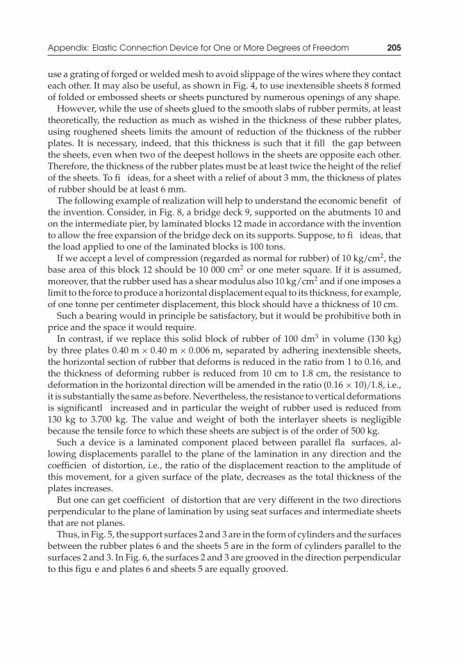
P1: TIX/XYZ P2: ABCJWST069-APP JWST069-Kelly-Style2 July 12, 2011 9:4 Printer Name: Yet to Come
Appendix: Elastic Connection Device for One or More Degrees of Freedom 205
use a grating of forged or welded mesh to avoid slippage of the wires where they contacteach other. It may also be useful, as shown in Fig. 4, to use inextensible sheets 8 formedof folded or embossed sheets or sheets punctured by numerous openings of any shape.
However, while the use of sheets glued to the smooth slabs of rubber permits, at leasttheoretically, the reduction as much as wished in the thickness of these rubber plates,using roughened sheets limits the amount of reduction of the thickness of the rubberplates. It is necessary, indeed, that this thickness is such that it fill the gap betweenthe sheets, even when two of the deepest hollows in the sheets are opposite each other.Therefore, the thickness of the rubber plates must be at least twice the height of the reliefof the sheets. To fi ideas, for a sheet with a relief of about 3 mm, the thickness of platesof rubber should be at least 6 mm.
The following example of realization will help to understand the economic benefit ofthe invention. Consider, in Fig. 8, a bridge deck 9, supported on the abutments 10 andon the intermediate pier, by laminated blocks 12 made in accordance with the inventionto allow the free expansion of the bridge deck on its supports. Suppose, to fi ideas, thatthe load applied to one of the laminated blocks is 100 tons.
If we accept a level of compression (regarded as normal for rubber) of 10 kg/cm2, thebase area of this block 12 should be 10 000 cm2 or one meter square. If it is assumed,moreover, that the rubber used has a shear modulus also 10 kg/cm2 and if one imposes alimit to the force to produce a horizontal displacement equal to its thickness, for example,of one tonne per centimeter displacement, this block should have a thickness of 10 cm.
Such a bearing would in principle be satisfactory, but it would be prohibitive both inprice and the space it would require.
In contrast, if we replace this solid block of rubber of 100 dm3 in volume (130 kg)by three plates 0.40 m × 0.40 m × 0.006 m, separated by adhering inextensible sheets,the horizontal section of rubber that deforms is reduced in the ratio from 1 to 0.16, andthe thickness of deforming rubber is reduced from 10 cm to 1.8 cm, the resistance todeformation in the horizontal direction will be amended in the ratio (0.16 × 10)/1.8, i.e.,it is substantially the same as before. Nevertheless, the resistance to vertical deformationsis significantl increased and in particular the weight of rubber used is reduced from130 kg to 3.700 kg. The value and weight of both the interlayer sheets is negligiblebecause the tensile force to which these sheets are subject is of the order of 500 kg.
Such a device is a laminated component placed between parallel fla surfaces, al-lowing displacements parallel to the plane of the lamination in any direction and thecoefficien of distortion, i.e., the ratio of the displacement reaction to the amplitude ofthis movement, for a given surface of the plate, decreases as the total thickness of theplates increases.
But one can get coefficient of distortion that are very different in the two directionsperpendicular to the plane of lamination by using seat surfaces and intermediate sheetsthat are not planes.
Thus, in Fig. 5, the support surfaces 2 and 3 are in the form of cylinders and the surfacesbetween the rubber plates 6 and the sheets 5 are in the form of cylinders parallel to thesurfaces 2 and 3. In Fig. 6, the surfaces 2 and 3 are grooved in the direction perpendicularto this figu e and plates 6 and sheets 5 are equally grooved.
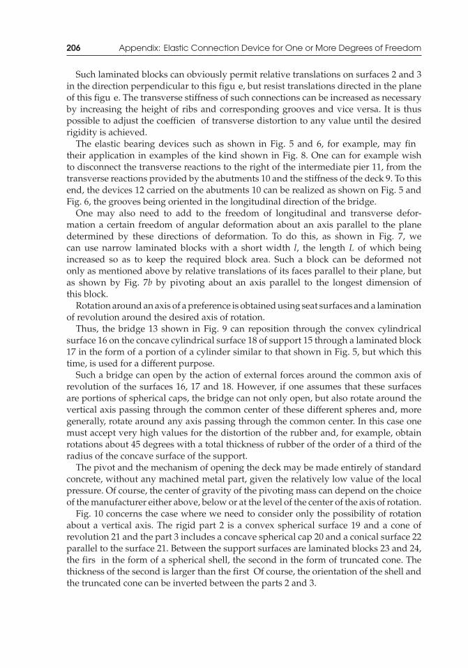
P1: TIX/XYZ P2: ABCJWST069-APP JWST069-Kelly-Style2 July 12, 2011 9:4 Printer Name: Yet to Come
206 Appendix: Elastic Connection Device for One or More Degrees of Freedom
Such laminated blocks can obviously permit relative translations on surfaces 2 and 3in the direction perpendicular to this figu e, but resist translations directed in the planeof this figu e. The transverse stiffness of such connections can be increased as necessaryby increasing the height of ribs and corresponding grooves and vice versa. It is thuspossible to adjust the coefficien of transverse distortion to any value until the desiredrigidity is achieved.
The elastic bearing devices such as shown in Fig. 5 and 6, for example, may fintheir application in examples of the kind shown in Fig. 8. One can for example wishto disconnect the transverse reactions to the right of the intermediate pier 11, from thetransverse reactions provided by the abutments 10 and the stiffness of the deck 9. To thisend, the devices 12 carried on the abutments 10 can be realized as shown on Fig. 5 andFig. 6, the grooves being oriented in the longitudinal direction of the bridge.
One may also need to add to the freedom of longitudinal and transverse defor-mation a certain freedom of angular deformation about an axis parallel to the planedetermined by these directions of deformation. To do this, as shown in Fig. 7, wecan use narrow laminated blocks with a short width l, the length L of which beingincreased so as to keep the required block area. Such a block can be deformed notonly as mentioned above by relative translations of its faces parallel to their plane, butas shown by Fig. 7b by pivoting about an axis parallel to the longest dimension ofthis block.
Rotation around an axis of a preference is obtained using seat surfaces and a laminationof revolution around the desired axis of rotation.
Thus, the bridge 13 shown in Fig. 9 can reposition through the convex cylindricalsurface 16 on the concave cylindrical surface 18 of support 15 through a laminated block17 in the form of a portion of a cylinder similar to that shown in Fig. 5, but which thistime, is used for a different purpose.
Such a bridge can open by the action of external forces around the common axis ofrevolution of the surfaces 16, 17 and 18. However, if one assumes that these surfacesare portions of spherical caps, the bridge can not only open, but also rotate around thevertical axis passing through the common center of these different spheres and, moregenerally, rotate around any axis passing through the common center. In this case onemust accept very high values for the distortion of the rubber and, for example, obtainrotations about 45 degrees with a total thickness of rubber of the order of a third of theradius of the concave surface of the support.
The pivot and the mechanism of opening the deck may be made entirely of standardconcrete, without any machined metal part, given the relatively low value of the localpressure. Of course, the center of gravity of the pivoting mass can depend on the choiceof the manufacturer either above, below or at the level of the center of the axis of rotation.
Fig. 10 concerns the case where we need to consider only the possibility of rotationabout a vertical axis. The rigid part 2 is a convex spherical surface 19 and a cone ofrevolution 21 and the part 3 includes a concave spherical cap 20 and a conical surface 22parallel to the surface 21. Between the support surfaces are laminated blocks 23 and 24,the firs in the form of a spherical shell, the second in the form of truncated cone. Thethickness of the second is larger than the first Of course, the orientation of the shell andthe truncated cone can be inverted between the parts 2 and 3.
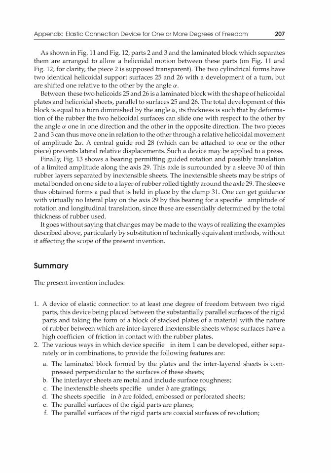
P1: TIX/XYZ P2: ABCJWST069-APP JWST069-Kelly-Style2 July 12, 2011 9:4 Printer Name: Yet to Come
Appendix: Elastic Connection Device for One or More Degrees of Freedom 207
As shown in Fig. 11 and Fig. 12, parts 2 and 3 and the laminated block which separatesthem are arranged to allow a helicoidal motion between these parts (on Fig. 11 andFig. 12, for clarity, the piece 2 is supposed transparent). The two cylindrical forms havetwo identical helicoidal support surfaces 25 and 26 with a development of a turn, butare shifted one relative to the other by the angle α.
Between these two helicoids 25 and 26 is a laminated block with the shape of helicoidalplates and helicoidal sheets, parallel to surfaces 25 and 26. The total development of thisblock is equal to a turn diminished by the angle α, its thickness is such that by deforma-tion of the rubber the two helicoidal surfaces can slide one with respect to the other bythe angle α one in one direction and the other in the opposite direction. The two pieces2 and 3 can thus move one in relation to the other through a relative helicoidal movementof amplitude 2α. A central guide rod 28 (which can be attached to one or the otherpiece) prevents lateral relative displacements. Such a device may be applied to a press.
Finally, Fig. 13 shows a bearing permitting guided rotation and possibly translationof a limited amplitude along the axis 29. This axle is surrounded by a sleeve 30 of thinrubber layers separated by inextensible sheets. The inextensible sheets may be strips ofmetal bonded on one side to a layer of rubber rolled tightly around the axle 29. The sleevethus obtained forms a pad that is held in place by the clamp 31. One can get guidancewith virtually no lateral play on the axis 29 by this bearing for a specifie amplitude ofrotation and longitudinal translation, since these are essentially determined by the totalthickness of rubber used.
It goes without saying that changes may be made to the ways of realizing the examplesdescribed above, particularly by substitution of technically equivalent methods, withoutit affecting the scope of the present invention.
Summary
The present invention includes:
1. A device of elastic connection to at least one degree of freedom between two rigidparts, this device being placed between the substantially parallel surfaces of the rigidparts and taking the form of a block of stacked plates of a material with the natureof rubber between which are inter-layered inextensible sheets whose surfaces have ahigh coefficien of friction in contact with the rubber plates.
2. The various ways in which device specifie in item 1 can be developed, either sepa-rately or in combinations, to provide the following features are:
a. The laminated block formed by the plates and the inter-layered sheets is com-pressed perpendicular to the surfaces of these sheets;
b. The interlayer sheets are metal and include surface roughness;c. The inextensible sheets specifie under b are gratings;d. The sheets specifie in b are folded, embossed or perforated sheets;e. The parallel surfaces of the rigid parts are planes;f. The parallel surfaces of the rigid parts are coaxial surfaces of revolution;
P1: TIX/XYZ P2: ABCJWST069-APP JWST069-Kelly-Style2 July 12, 2011 9:4 Printer Name: Yet to Come
208 Appendix: Elastic Connection Device for One or More Degrees of Freedom
g. The parallel surfaces of the rigid parts are helicoidal surfaces of the same axis andthe same pitch;
h. The parallel surfaces of the rigid parts are concentric spherical caps;i. The parallel surfaces of rigid parts have on one part, at least one rib and on the
other at least one groove corresponding to that rib allowing them to nest into oneanother;
j. The laminated block includes plates and sheets of rectangular shape, of whichthe length far exceeds the width, with its greatest dimension, directed along aneventual axis of rotation;
k. The laminated block is obtained by the simultaneous winding of a metal strip anda strip of rubber which are bonded to each other around a cylindrical surface.
3. The application of these elastic connections, as specifie in items 1 and 2, to structuresthat can move with respect to their supports, and especially to bridges, are for theprovision of supports allowing expansion, or to allow the displacement of thesestructures with the help of external forces.
4. The application of these devices of elastic connection, as specifie in items 1 and 2,with mechanical precision to two parts with a view to allow for relative displacements,limited but guided, of the two parts with respect to each other.
P1: TIX/XYZ P2: ABCJWST069-REF JWST069-Kelly-Style2 July 27, 2011 12:48 Printer Name: Yet to Come
References
Anderson, T. L. (1989). “Seismic Isolation for the Los Angeles County Fire Command and ControlFacility.” Proceedings of the Structures Congress of the American Society of Civil Engineers, Vol. 1,pp 615–624. San Francisco, California, May 1–5, 1989.
Bouchon, M. (1988). “Nuclear Spent Fuel Storage Pools on Aseismic Bearing Pads.” Proceedings ofthe Ninth World Conference on Earthquake Engineering (9WCEE), Vol V, pp 533–538. Tokyo-Kyoto,Japan, August 2–9, 1988.
Chalhoub, M. S. and Kelly, J. M. (1987). “Reduction of the Stiffness of Rubber Bearings due toCompressibility.” Report No. UCB/SEMM-86/06, Department of Civil Engineering, University ofCalifornia, Berkeley.
Chalhoub, M. S. and Kelly, J. M. (1991). “Analysis of Infinite-Strip-Shape Base Isolatorwith Elastomer Bulk Compression.” Journal of Engineering Mechanics (ASCE), 117(8), 1791–1805.
Constantinou M. C., Kartoum A., and Kelly, J. M. (1992). “Analysis of Compression of HollowCircular Elastomeric Bearings.” Engineering Structures, 14(2), 103–111.
Crockett, J. H. A. (1983). “Early Attempts, Research and Modern Techniques for InsulatingBuildings.” Proceedings of the International Conference on Natural Rubber for Earthquake Protec-tion of Buildings and Vibration Isolation, pp 15–44. Kuala Lumpur, Malaysia, February 22–25,1982.
Derham, C. J. and Kelly, J. M. (1985). “Combined Earthquake Protection and Vibration Isolationof Structures.” Natural Rubber Technology, 16, 3–11.
Derham, C. J. and Waller, R. A. (1975). “Luxury without Rumble.” The Consulting Engineer, 39(7),49–53.
Fuller, K. N. G., Gregory, M. J., Harris, J. A., Muhr, A. H., Roberts, A. D., and Sevenson, A.(1988), “Engineering Use of Natural Rubber.” In: Roberts, A. D., ed. Natural Rubber Science andTechnology, Oxford University Press, New York, New York.
Freyssinet, E. (1954). “Dispositif de liaison elastique a un ou plusieurs degres de liberte” (translatedas “Elastic Device of Connection to One or More Degrees of Freedom”), French patent no.1.110.285 Class F06 d 25/5/54, Ministry of Industry and Commerce, France.
Freyssinet International (1977). “Congress Centre in Berlin.” Freyssinet International, Vol. 159.Garevski, M., Kelly, J. M., and Bojadziev, M. (1998). “Experimental Dynamic Testing of the First
Structure in the World Isolated by Rubber Bearings.” Proceedings of the Eleventh European Con-ference on Earthquake Engineering. Paris, France, September 6–11, 1998.
Mechanics of Rubber Bearings for Seismic and Vibration Isolation, First Edition. James M. Kelly and Dimitrios A. Konstantinidis.C© 2011 John Wiley & Sons, Ltd. Published 2011 by John Wiley & Sons, Ltd.
209
P1: TIX/XYZ P2: ABCJWST069-REF JWST069-Kelly-Style2 July 27, 2011 12:48 Printer Name: Yet to Come
210 References
Gent, A. N. (1964). “Elastic Stability of Rubber Compression Springs.” Journal of Mechanical Engi-neering Science, 6(4), 318–326.
Gent, A. N. (1990). “Cavitation in Rubber: A Cautionary Tale.” Rubber Chemistry and Technology,63, G49–G53.
Gent, A. N. (2001). “Elasticity.” In: Gent A. N., ed. Engineering with Rubber: How to Design RubberComponents, 2nd edn, Hanser Gardner, Cincinnati, Ohio.
Gent, A. N. and Lindley, P. B. (1959a). “Internal Rupture of Bonded Rubber Cylinders in Tension.”Proceeding of the Royal Society of London, Ser. A, 249, 195–205.
Gent, A. N. and Lindley, P. B. (1959b). “The Compression of Bonded Rubber Blocks.” Proceedingsof the Institution of Mechanical Engineers, 173(3), 111–122.
Gent, A. N. and Meinecke, E. A. (1970). “Compression, Bending and Shear of Bonded RubberBlocks.” Polymer Engineering and Science, 10(1), 48–53.
Grootenhuis, P. (1983). “Vibration isolation of buildings—some basic principles.” Proceedings ofthe International Conference on Natural Rubber for Earthquake Protection of Buildings and VibrationIsolation, pp 1–14. Kuala Lumpur, Malaysia, 1982.
Haringx, J. A. (1949). “On Highly Compressible Helical Springs and Rubber Rods, and TheirApplication for Vibration-Free Mountings, III.” Philips Research Reports, 4, 206–220.
HKS (2001). ABAQUS, Version 6.2 [computer software]. Hibbitt, Karlsson & Sorensen Inc.,Pawtucket, Rhode Island.
ICC (2009). 2009 International Building Code (IBC 2009), International Code Council (ICC),Washington, D.C.
Kamada, T. and Fujita, T. (2007). “Current Status of Seismic Isolation and Vibration Control toBuildings, Cultural Heritage and Industrial Facilities in Japan.” Proceedings of the ASSISi 10thWorld Conference on Seismic Isolation, Energy Dissipation and Active Vibrations Control of Structures.Istanbul, Turkey, May 28–31, 2007.
Kelly, J. M. (1991). “Dynamic and Failure Characteristics of Bridgestone Isolation Bearings.”ReportNo. UCB/EERC-1991/04, Earthquake Engineering Research Center, University of California,Berkeley.
Kelly, J. M. (1997). Earthquake-Resistant Design with Rubber, 2nd edn, Springer-Verlag, London,England.
Kelly, J. M. (2003). “Tension Buckling in Multilayer Elastomeric Bearings.” Journal of EngineeringMechanics (ASCE), 129(12), 1363–1368.
Kelly, J. M. and Konstantinidis, D. (2007). “Low-Cost Seismic Isolators for Housing in Highly-Seismic Developing Countries.” Proceedings of the ASSISi 10th World Conference on Seismic Isola-tion, Energy Dissipation and Active Vibrations Control of Structures. Istanbul, Turkey, May 28–31,2007.
Kelly, J. M. and Konstantinidis, D. (2009a). “Steel Shim Stresses in Multilayer Bearings underCompression and Bending.” Journal of Mechanics of Materials and Structures, 4(6), 1109–1125.
Kelly, J. M. and Konstantinidis, D. (2009b). “Effect of Friction on Unbonded Elastomeric Bearings.”Journal of Engineering Mechanics (ASCE), 135(9), 953–960.
Kelly, J. M. and Takhirov, S. M. (2001). “Analytical and Experimental Study of Fiber-ReinforcedElastomeric Isolators.” Report No. PEER-2001/11, Pacifi Earthquake Engineering Research Cen-ter, University of California, Berkeley.
Kelly, J. M. and Takhirov, S. M. (2004). “Analytical and Numerical Study on Buckling of ElastomericBearings with Various Shape Factors.” Report No. UCB/EERC-2004/03, Earthquake EngineeringResearch Center, University of California, Berkeley.
Kelly, J. M. and Takhirov, S. M. (2007). “Tension Buckling in Multilayer Elastomeric IsolationBearings.” Journal of Mechanics of Materials and Structures, 2(8), 1591–1605.
P1: TIX/XYZ P2: ABCJWST069-REF JWST069-Kelly-Style2 July 27, 2011 12:48 Printer Name: Yet to Come
References 211
Kircher, C. A., Delfosse, G. C., Schoof, C. C., Khemici, O., and Shah, H. C. (1979). “Perfor-mance of a 230 KV ATB 7 Power Circuit Breaker Mounted on GAPEC Seismic Isolators.”Report No. JABEEC 40, The John A. Blume Earthquake Engineering Center, Stanford University,California.
Koh, C. G. and Kelly, J. M. (1987). “Effects of Axial Load on Elastomeric Isolation Bearings.”ReportNo. UCB/EERC-1986/12, Earthquake Engineering Research Center, University of California,Berkeley.
Konstantinidis, D., Kelly, J. M., and Makris, N. (2008). “Experimental Investigation on the SeismicResponse of Bridge Bearings.”Report No. UCB/EERC-2008/02, Earthquake Engineering ResearchCenter, University of California, Berkeley.
Lindley, P. B. (1966). “Load-Compression Relationships of Rubber Units.” Journal of Strain Analysis,1(3), 190–195.
Lindley, P. B. (1978). “Engineering Design with Natural Rubber.” NR Technical Bulletin, 4th edn,The Malaysian Rubber Producers’ Research Association, Brickendonbury, Hertford, England.
McLachlan, N. W. (1955).Bessel Functions for Engineers, 2nd edn, Clarendon Press, Oxford, England.Naeim, F. and Kelly, J. M. (1999). Design of Seismic Isolated Structures: From Theory to Practice,
John Wiley & Sons, New York, New York.Plichon, C., Gueraud, R., Richli, M. H., and Casagrande, J. F. (1980). “Protection of Nuclear Power
Plants against Seism.” Nuclear Technology, 49(2), 295–306.Postollec, J.-C. (1982). “Les Fondations Antisismiques de la Centrale Nucleaire de Cruas-Meysse.”Travaux, No. 569, September, pp 75–83.
Prager, W. and Hodge, P. G. (1951), Theory of Perfectly Plastic Solids, John Wiley & Sons, New York,New York.
Renault, J., Richli, M., and Pavot, B. (1979). “Premiere Application des Appuis Anti-Sismiquesa Friction: La Centrale Nucleaire de Koeberg” (translated as “First Application of AntiseismicFriction Bearings: Koeberg Nuclear Plant”). Annales de l’Institut Technique du Batiment et desTravaux Publics, No. 371, pp 69–90.
Rocard, Y. (1937). “Note sur le Calcul des Proprietes Elastique des Supports en Caoutchouc Adherent”Journal de Physique et de Radium, 8, 197–203.
Snowden, J. C. (1979). “Vibration Isolation: Use and Characterization.” NBS Handbook 128, U.S.National Bureau of Standards, Washington, DC.
Taniwangsa, W., Clark, P. W., and Kelly, J. M. (1996). “Natural Rubber Isolation Systems for Earth-quake Protection of Low-Cost Buildings.”ReportNo. UCB/EERC-95/ 12, Earthquake EngineeringResearch Center, University of California, Berkeley.
Tarics, A. G., Way, D., and Kelly, J. M. (1984). “The Implementation of Base Isolation for theFoothill Communities Law and Justice Center.” Report to the National Science Foundation and theCounty of San Bernardino, Base Isolation Consultants Inc., San Francisco, California.
Terashima, N. and Miyazaki, M. (2001). “Design Example of Base-Isolated Artificia Ground.”Kenchiku-Gijutsu, 172–175 (in Japanese).
Timoshenko, S. P. and Goodier, J. N. (1970). Theory of Elasticity, 3rd edn, McGraw-Hill, New York,New York.
Tsai, H.-C. and Kelly, J. M. (2002). “Stiffness Analysis of Fiber-Reinforced Rectangular SeismicIsolators.” Journal of Engineering Mechanics (ASCE), 128(4), 462–470.
Tyler, R. G. (1991). “Rubber Bearings in Base-Isolated Structures: A Summary Paper.” Bulletin ofthe New Zealand National Society for Earthquake Engineering, 24(3), 251–274.
Walters, M. T., Honeck, B., and Elsesser, E. (1995). “Use of Seismic Isolation in New andRetrofi Construction.” Proceedings of the Joint ASME/JSMR Pressure Vessels and Piping Confer-ence, pp 221–228. Honolulu, Hawaii, July 23–27, 1995.

P1: TIX/XYZ P2: ABCJWST069-REF JWST069-Kelly-Style2 July 27, 2011 12:48 Printer Name: Yet to Come
212 References
Weisstein, E. W. (2002). CRC Concise Encyclopedia of Mathematics, 2nd edn, Chapman & Hall/CRC,Boca Raton, Florida.
Yang, T. Y., Konstantinidis, D., and Kelly, J. M. (2010). “The Influenc of Isolator Hysteresis onEquipment Performance in Seismic Isolated Buildings.” Earthquake Spectra, 26(1), 275–293.
Youssef, N. (2001). “Viscous Dampers at Multiple Levels for the Historic Preservation of LosAngeles City Hall.” The Structural Design of Tall Buildings, 10(5), 339–350.

P1: TIX/XYZ P2: ABCJWST069-PHOTO-CREDIT JWST069-Kelly-Style2 July 27, 2011 12:52 Printer Name: Yet to Come
Photograph Credits
The authors are grateful for permission to reproduce photographs for the followingfig res.
1.1 By Hans-Georg Weimar. License: Creative Commons Attribution Version 2.0Germany. Accessed November 19, 2010, http://commons.wikimedia.org/wiki/File:ICC_Berlin_pixelquelle.jpg.
1.2 Reproduced by permission of Freyssinet, Inc.1.3 Courtesy of James M. Kelly. NISEE Online Archive, University of California,
Berkeley.1.4 Courtesy of James M. Kelly. NISEE Online Archive, University of California,
Berkeley.1.5 Courtesy of James M. Kelly. NISEE Online Archive, University of California,
Berkeley.1.6 Courtesy of James M. Kelly. NISEE Online Archive, University of California,
Berkeley.1.7 Courtesy of James M. Kelly. NISEE Online Archive, University of California,
Berkeley.1.8 Courtesy of James M. Kelly. University of California, Berkeley.1.9 By Brion Vibber. Licensed: Creative Commons Attribution-Share Alike 1.0
Generic license. Accessed December 21, 2010, http://upload.wikimedia.org/wikipedia/commons/4/48/Los_Angeles_City_Hall_%28color%29_edit1.jpg.
1.10 Courtesy of James M. Kelly. University of California, Berkeley.1.11 Courtesy of Ian D. Aiken. SIE, Inc.1.12 Courtesy of James M. Kelly. University of California, Berkeley.1.13 Courtesy of James M. Kelly. University of California, Berkeley.1.14 Courtesy of James M. Kelly. University of California, Berkeley.
Mechanics of Rubber Bearings for Seismic and Vibration Isolation, First Edition. James M. Kelly and Dimitrios A. Konstantinidis.C© 2011 John Wiley & Sons, Ltd. Published 2011 by John Wiley & Sons, Ltd.
213

P1: TIX/XYZ P2: ABCJWST069-PHOTO-CREDIT JWST069-Kelly-Style2 July 27, 2011 12:52 Printer Name: Yet to Come

P1: TIX/XYZ P2: ABCJWST069-AUIND JWST069-Kelly-Style2 July 28, 2011 0:12 Printer Name: Yet to Come
Author Index
Anderson, 7
Bouchon, 16
Chalhoub, 33, 40Constantinou, 40Crockett, 2
Derham, 2, 6
Freyssinet, 1, 159, 173Fujita, 13Fuller, 44
Garevski, 4Gent, 20, 83, 109, 119, 122, 129Goodier, 65, 68, 70–1Grootenhuis, 2
Haringx, 83, 129Hodge, 78
Kamada, 13Kelly, 4, 6, 14–15, 33, 40, 63–4, 82, 91, 103,
108–9, 113, 116, 120, 127–8, 130, 159,177–8, 192
Kircher, 90Koh, 91, 103, 108Konstantinidis, 63–4, 82, 159, 177, 179, 182,
184, 192
Lindley, 20, 35, 44, 109
McLachlan, 81Meinecke, 20Miyazaki, 13
Naeim, 4
Postollec, 16Prager, 78
Renault, 16Rocard, 20
Snowden, 2
Takhirov, 120, 127–8Taniwangsa, 14–15Tarics, 6Terashima, 13Timoshenko, 65, 68, 70–1Tsai, 130Tyler, 90
Waller, 2Walters, 8, 10Weisstein, 165
Yang, 16Youssef, 10
Mechanics of Rubber Bearings for Seismic and Vibration Isolation, First Edition. James M. Kelly and Dimitrios A. Konstantinidis.C© 2011 John Wiley & Sons, Ltd. Published 2011 by John Wiley & Sons, Ltd.
215

P1: TIX/XYZ P2: ABCJWST069-AUIND JWST069-Kelly-Style2 July 28, 2011 0:12 Printer Name: Yet to Come
P1: TIX/XYZ P2: ABCJWST069-IND JWST069-Kelly-Style2 July 28, 2011 2:37 Printer Name: Yet to Come
Subject Index
ABAQUS, 120–2Aktins Research and Development, 2anti-vibration mounts, 2average shear strain, 32
circular pad, 33infinit strip pad, 33
bearingsbonding requirements, 177bridge bearings, 5, 179–81, 184
thermal expansion, 192computer modelling, 100constrained by friction, 1dowelled, 108–9end-plates, 177–80
thickness of, 179enhanced stability bearings, 90finit element model of, 114, 120–1high-damping natural rubber, 6, 8, 10, 12,
14–15history of multilayer rubber
bearings, 1low-cost applications, 130, 156manufacturing process, 178natural rubber, 2, 4, 7, 11, 17–18
mechanical dampers, 12tensile stresses in, 177–81treated as composite beams, 130typical costs of isolators, 178typical diameters, 129typical heights, 129typical weights, 129
unbonded bearingsdesirable characteristics for low-cost
seismic isolation, 192effect of frictional restraint, 177typical geometrical characteristics, 182ultimate lateral displacement, 177, 180vertical stiffness, see vertical stiffness
bendingboundary value problem, 47incompressibility condition, 46–7rubber pads with compressible rubber, of, 52
annular pad, 58circular pad, 54infinit strip pad, 52rectangular pad, 57
rubber pads with incompressible rubber, of,45
annular pad, 51circular pad, 48infinit strip pad, 47rectangular pad, 49
bending stiffness, 45, 47–8compressible rubber
annular pad, 60circular pad, 55infinit strip pad, 53rectangular pad, 58
compressible/incompressible ratioannular pad, 61circular pad, 56infinit strip pad, 53rectangular pad, 58
Mechanics of Rubber Bearings for Seismic and Vibration Isolation, First Edition. James M. Kelly and Dimitrios A. Konstantinidis.C© 2011 John Wiley & Sons, Ltd. Published 2011 by John Wiley & Sons, Ltd.
217
P1: TIX/XYZ P2: ABCJWST069-IND JWST069-Kelly-Style2 July 28, 2011 2:37 Printer Name: Yet to Come
218 Subject Index
bending stiffness (Continued )incompressible rubber
annular pad, 51circular pad, 48infinit strip pad, 48rectangular pad, 50
bending strain, 64body forces, 63
in-plane, 65per unit volume, 67
bonding compounds, 173bonding requirements, 177, 181bridge supports, 159Bridgestone Engineered Products Co., 8, 13British Nuclear Fuels, 17buckling
analysis for bearings with flexibl shims(inc. warping), 146
annular bearings, of, 90–1boundary conditions, 87, 92circular bearings, of, 83critical load, 88, 90
effect of compressibility on, 110effect of shape factor on, 122, 126effect of shortening, 128influenc of plate flexibilit on, 129influenc of shim thickness on, 156
critical load (dynamic), 108critical pressure, 89effect of rubber compressibility on, 110Euler load, 88in tension
critical load, 114effect of lengthening on, 128
finit element models of, 120numerical modelling of, 120postbuckling behavior, 122
of short beams (inc. warping), 139safety factor, 89–91
buckling load, see buckling, critical loadbulk compressibility, 33, 35, 37, 39–43, 52, 62,
80, 110–11bulk modulus, 33, 39–40, 44, 111
cavitation, 119–20Central Electricity Generating Board, 17Central Research Institute of Electric Power
Industry, 17COGEMA, 16
compressionboundary value problem, 23incompressibility constraint, 80incompressibility condition, 23max shear stresses produced
circular pad, 32infinit strip pad, 31
infinit strip bearings with incompressiblerubber, of, 184
rubber pads with compressible rubber, of, 33annular pad, 40circular pad, 36infinit strip pad, 33rectangular pad, 39
rubber pads with incompressible rubber, of,19
annular pad, 27circular pad, 25infinit strip pad, 24rectangular pad, 26
shear stresses produced by, 30unbonded rubber pads with incompressible
rubber, 160circular pad, 169infinit strip pad, 163
yielding of shims under, 78influenc of bulk compressibility, 80
compression modulus, 20, 27–9, 35, 37–9, 42–4,118–19
compressible rubberannular pad, 40circular pad, 35, 65, 81infinit strip pad, 34rectangular pad, 37
incompressible rubberannular pad, 28circular pad, 25, 64infinit strip pad, 25rectangular pad, 27unbonded circular pad, 173unbonded infinit strip bearing, 190unbonded infinit strip pad, 168
compression strain, 22, 31Cramer’s rule, 136, 144curvature, 84
dampingin an isolation system, 4influenc of compressive load on, 106
P1: TIX/XYZ P2: ABCJWST069-IND JWST069-Kelly-Style2 July 28, 2011 2:37 Printer Name: Yet to Come
Subject Index 219
deformationassumption, in buckling theory, 83isolation system, 4, 16kinematic variables (buckling), 86structure, 4
deviatoric strain invariants, 121displacement
downward displacement of top of a bearing,95–6, 103
upward displacement of top of a bearing,117
displacement fielbending, 45buckling, 83buckling (inc. warping), 131compression, 21compression (inc. slip), 163, 169, 185
earthquakeKobe (1995), 13Loma Prieta (1989), 9, 11Northridge (1994), 8, 10San Francisco (1906), 11
Earthquake Engineering Research Center, 4,14, 108
earthquake-resistant design, 11elastic volume ratio, 121Electricite de France, 16elongation to break, 32equilibrium equations, 22, 46, 130, 133, 140,
161, 163, 170, 187Euler load, see bucklingexternal work, 32
fixed-bas period, 178Fourier series, 26, 39, 49, 57friction, 159, 177
coefficient 161, 168, 173–4, 188–9effect of on unbonded rubber pads, see
compression modulus and pressuresolution
GERB, 17ground motion, 2, 4, 11, 13
hardness, 180horizontal frequency, 89, 91horizontal stiffness, 89
dynamic, 107effect of tensile vertical load on, 115
effect of vertical load on, 115function of vertical load, as, 91, 100reduction of, 16
hydrostatic, 119hyperelastic, 121
incompressibility, 21, 33, 35, 42, 63–4, 68,160
incompressibility condition, 23, 184instability, see bucklinginternal work, 95isolated ground, 13isolator, see bearings
Japanese Ministry of International Trade andIndustry, 17
Lambert W function, 165–6, 172loose bolts, 119loss angle, 106loss factor, 106–7lubrication, 184
Malaysian Rubber Producers’ ResearchAssociation, 2, 14
modifie Bessel equation, 36, 40modifie Bessel function, 36, 38–40, 42, 55–6,
60, 65, 81
Neo-Hookean, 122, 127Neoprene, 180normalized pressure distribution, 35–6nuclear power plants, 15
fast breeder reactors (FBR), 17floo spectra, 16piping systems
multiple input spectra, for, 16
overlap area, 180overturning moment, 119
plane stress, 63, 65, 68Poisson ratio, 68, 121, 152polychloroprene, 119, 180polyisoprene, 119polynomial, 121–2, 127postbuckling behavior, 100, 104, 122,
126potential, 63, 67, 73
P1: TIX/XYZ P2: ABCJWST069-IND JWST069-Kelly-Style2 July 28, 2011 2:37 Printer Name: Yet to Come
220 Subject Index
pressure solutionbending
compressible rubberannular pad, 55circular pad, 60, 65infinit strip pad, 53rectangular pad, 57
incompressible rubberannular pad, 51circular pad, 48, 64infinit strip pad, 47rectangular pad, 50
compressioncompressible rubber
annular pad, 40circular pad, 36, 65infinit strip pad, 33rectangular pad, 39
incompressible rubberannular pad, 28circular pad, 25, 64infinit strip pad, 24rectangular pad, 27unbonded bearing, 189–90unbonded circular pad, 171unbonded infinit strip pad,
167continuity of, 165, 171–2, 187,
189–90stress assumption, 22
radius of the curvature, 46recessed end-plate connection, 15resonance, 4retrofi
of buildings using isolation, 8–11Richter magnitude, 6, 8roll-off, 179, 181–2rollout stability, 108–9
maximum displacement, 108rotation, 46, 76rubber rods, 83, 129
safety factor, 89–91San Andreas fault, 6Scougal Rubber Corporation, 180second shape factor, see shape factorseismic isolator, see bearings
seismic gap, 9, 14seismic isolation
cost of, 4, 6–8delicate equipment, protection of, 2developing countries, in, 178, 192life-cycle costs, 8low-cost isolation systems, 13
seismically isolated buildingUnited States
Arrowhead Regional Medical Center, 8Los Angeles City Hall, 9–10Oakland City Hall, 8–9San Francisco City Hall, 9, 11St. Johns Medical Center, 8University of Southern California
Teaching hospital, 8seismically isolated buildings
demonstration buildings, 14China, 14Indonesia, 14–15Japan, 12
JapanMinistry of Construction, 11West Japan Postal Computer Center, 13
MacedoniaPestalozzi elementary school, 4–5
United StatesCaltrans/CHP Traffi Management
Center, 8Emergency Operations Center, 8Fire Command and Control Facility, 6–7Foothill Communities Law and Justice
Center, 6–7Hearst Memorial Mining Building, 11–12Martin Luther King Jr. Civic Center, 11Martin Luther King Jr./C.R. Drew
Medical Center, 8seismically isolated nuclear power plants
Cruas (France), 16–17Koeberg (South Africa), 16standardized plant design, 16–17
shape factor, 20annular pad, 20circular pad, 20infinit strip, 20rectangular pad, 20second, 89
shear force, internal, 83
P1: TIX/XYZ P2: ABCJWST069-IND JWST069-Kelly-Style2 July 28, 2011 2:37 Printer Name: Yet to Come
Subject Index 221
shear modulus, 23shear strains, 23, 30, 44shear stressalso see compression, shear stresses
produced byin-plane, 22
shims, 1, 19, 63completely flexible 130, 177completely rigid, 130effect of plate flexibilit on buckling load, see
bucklingpressure to cause full yielding
in bearings with compressible rubber, 79in bearings with incompressible rubber,
78purpose of, 63stresses in, 53
for bearings with compressible rubber, 73under pure bending, 77under pure compression, 74
for bearings with incompressible rubber,65
under pure bending, 72under pure compression, 69
thickness, of, 67, 129, 178yielding under compression, 78
in bearings with compressible rubber, 79in bearings with incompressible rubber, 78
Shore A Scale, 180slip, 159, 163, 169
heat generated by, 182unbonded circular pad under compression,
in, 173unbonded infinit strip pad under
compression, in, 168Spie Batignolles, 16stability
multilayered rubber bearings, of, 83multilayered rubber springs (Gent), of, 83rollout, see rollout stabilitysolid rubber rods (Haringx), of, 83, 129
stored energy, 151–2strain energy potential, 121stress concentration, 70stress function, 63–6, 68, 71, 73–4, 76Struve functions, 81surface shear stresses, 65, 67surface shears, 63, 162
surface stresses, 186symmetry, 185, 187
tensile stresses, 177, 179–81bonding, 181
cost of, 181total elastic stored energy, 32Tresca yield condition, 78–80triaxial stress, 120Tun Abdul Razak Research Centre, 2, 14two-spring model, 100–1, 104, 106, 108
deformations, 102downward displacement, 102postbuckling behavior, 104vertical stiffness, 103
ultimate lateral displacement, see bearings,unbonded
unbalanced moment, 179–80unbonded pads
frictional restraint on, 159United Nations Industrial Development
Organization (UNIDO), 13–14, 130unreinforced masonry buildings, 14, 178
vertical frequency, 2, 19, 39vertical stiffness, 1, 19, 33, 44
as a function of horizontal displacement,99–100, 118
of two-spring model, see two-spring modelreduction of, due to slip, 184run-in effect, 19unbonded bearings, of, 177
vibration isolation, 1–2, 4, 18isolation of equipment, 2rail traffic 2vertical ground motion, 2
vibration-isolated buildingsGermany
International Congress Center (Berlin),2–3
United KingdomAlbany Court (London), 2Glasgow Royal Concert Hall, 2Grafton 16 public housing complex, 2Holiday Inn London, 2International Convention Center
(Birmingham), 2
P1: TIX/XYZ P2: ABCJWST069-IND JWST069-Kelly-Style2 July 28, 2011 2:37 Printer Name: Yet to Come
222 Subject Index
vibration-isolated buildings (Continued )United States
Benaroya Concert Hall (Seattle),4
Walt Disney Concert Hall (LostAngeles), 4
virtual workexternal, 134internal, 134
viscous dampers, 10, 17vulcanization, 1
warping, 130–2warping function, 130
yield stress, 70, 78yielding, see shims, yielding ofYoung’s modulus, 121, 152, 162, 189