metastability-containing circuits, parallel distance
TRANSCRIPT

Metastability-Containing Circuits,Parallel Distance Problems, and
Terrain Guarding
A dissertation submitted towards the degree Doctor of Engineeringof the Faculty of Mathematics and Computer Science of Saarland
University
by Stephan Friedrichs
Saarbrucken / 2017
Day of Colloquium: 11. September 2017Dean of the Faculty: Univ.-Prof. Dr. Frank-Olaf Schreyer
Chair of the Committee: Prof. Dr.-Ing. Holger HermannsReporters
First reviewer: Dr. Christoph LenzenSecond reviewer: Prof. Dr. Dr. h.c. mult. Kurt MehlhornThird reviewer: Prof. Dr. Mohsen Ghaffari
Academic Assistant: Dr. Emanuele Natale
ii

Abstract
“Don’t quote me on that!”
Christoph Lenzen
Abstract We study three problems. The first is the phenomenon of metastability indigital circuits. This is a state of bistable storage elements, such as registers, that isneither logical 0 nor 1 and breaks the abstraction of Boolean logic. We propose a time- andvalue-discrete model for metastability in digital circuits and show that it reflects relevantphysical properties. Further, we propose the fundamentally new approach of using logicalmasking to perform meaningful computations despite the presence of metastable upsetsand analyze what functions can be computed in our model. Additionally, we show thatcircuits with masking registers grow computationally more powerful with each availableclock cycle.
The second topic are parallel algorithms, based on an algebraic abstraction of theMoore-Bellman-Ford algorithm, for solving various distance problems. Our focus are dis-tance approximations that obey the triangle inequality while at the same time achievingpolylogarithmic depth and low work.
Finally, we study the continuous Terrain Guarding Problem. We show that it hasa rational discretization with a quadratic number of guard candidates, establish itsmembership in NP and the existence of a PTAS, and present an efficient implementationof a solver.
Zusammenfassung Wir betrachten drei Probleme, zunachst das Phanomen von Me-tastabilitat in digitalen Schaltungen. Dabei geht es um einen Zustand in bistabilenSpeicherelementen, z. B. Registern, welcher weder logisch 0 noch 1 entspricht und dieAbstraktion Boolescher Logik unterwandert. Wir prasentieren ein zeit- und wertdiskretesModell fur Metastabilitat in digitalen Schaltungen und zeigen, dass es relevante physi-kalische Eigenschaften abbildet. Des Weiteren prasentieren wir den grundlegend neuenAnsatz, trotz auftretender Metastabilitat mit Hilfe von logischem Maskieren sinnvolleBerechnungen durchzufuhren und bestimmen, welche Funktionen in unserem Modellberechenbar sind. Daruber hinaus zeigen wir, dass durch Maskingregister in zusatzlichenTaktzyklen mehr Funktionen berechenbar werden.
Das zweite Thema sind parallele Algorithmen die, basierend auf einer Algebraisierungdes Moore-Bellman-Ford-Algorithmus, diverse Distanzprobleme losen. Der Fokus liegtauf Distanzapproximationen unter Einhaltung der Dreiecksungleichung bei polylogarith-mischer Tiefe und niedriger Arbeit.
Abschließend betrachten wir das kontinuierliche Terrain Guarding Problem. Wirzeigen, dass es eine rationale Diskretisierung mit einer quadratischen Anzahl von Wachter-positionen erlaubt, folgern dass es in NP liegt und ein PTAS existiert und prasentiereneine effiziente Implementierung, die es lost.

iv

Acknowledgments
“Moin Jungs, zwei Caipis?”
The Feinkost barkeeper
I want to express my sincere gratitude to my advisor Christoph Lenzen. Thank youfor advising with ample patience, knowing when to ask new research questions andwhen to let me to pursue my own projects, and for making the Theory of Distributedand Embedded Systems group a wonderful place to work at, creating an atmosphere ofresearch, learning, writing, teaching, traveling, and various social activities. I’m indebtedto Kurt Mehlhorn for offering me a position at the Max Planck Institute for Informatics’Algorithms and Complexity group, it has been an incredibly rewarding time. I want tothank Mohsen Ghaffari for taking the time to be the external reviewer.
Out of my colleagues and friends at the MPI, I want to mention some in particular.Joel Rybicki, thanks for exploring the city with me, helping me figure out the tabs ofAny Other Day, and countless hot and cold beverages. Thank you Matthias Fugger forgreat research, living the culture of the research coffee, the afternoons with guitars inthe park, and numerous visits to Feinkost, Nautilus, Vienna and Paris. I wish to thankAttila Kinali for establishing the chocolate supply-chain, being a great office mate, livelydiscussions, and patiently explaining the dos and don’ts of digital circuit design to me.Moti Medina, thank you for great research, drinks and movies, and always knowing whichis advisable.
Regarding my time in Braunschweig, I want to thank my friend Christiane Schmidtfor always having an open ear, co-founding the research Friday, and all the support.Thank you Michael Hemmer, co-founder of the research Friday, for always having myback and being a great host, colleague, and friend. I also wish to thank my friend HenningHasemann for lots of hot and cold beverages and the music. To Alexander Kroller I owethanks for the support and for convincing me to take part in the teach4tu program.
I’m indebted to Christoph Lenzen, Matthias Fugger, Attila Kinali, Christiane Schmidt,Michael Hemmer, Christian Ikenmeyer, and Pavel Kolev for many helpful comments onthis thesis.
As important as a healthy professional environment is, it cannot substitute a stablepersonal environment, friends with open ears and good advice, and a supporting family.Hence, I want to thank my friends, Henning Gunther, Martin Wegner, Jaffi Schraderand Thomas Hoffmann, and my family, Frauke, Werner, Karsten and Bernhard.

vi
Contents
“The most merciful thing in the world, I think, is the inability of the humanmind to correlate all its contents.”
H. P. Lovecraft, The Call of Cthulhu
1 Introduction 1
2 Notation and Preliminaries 5
2.1 Algebraic Foundations . . . . . . . . . . . . . . . . . . . . . . . . . . . . 5
2.2 Probability Theory . . . . . . . . . . . . . . . . . . . . . . . . . . . . . . 8
I Metastability-Containing Circuits 11
3 Introduction 13
3.1 Our Contribution . . . . . . . . . . . . . . . . . . . . . . . . . . . . . . . 15
3.2 Related Work . . . . . . . . . . . . . . . . . . . . . . . . . . . . . . . . . 17
3.3 Notation and Preliminaries . . . . . . . . . . . . . . . . . . . . . . . . . 19
4 Circuit Model 21
4.1 Registers . . . . . . . . . . . . . . . . . . . . . . . . . . . . . . . . . . . . 23
4.2 Gates . . . . . . . . . . . . . . . . . . . . . . . . . . . . . . . . . . . . . 25
4.3 Combinational Logic . . . . . . . . . . . . . . . . . . . . . . . . . . . . . 26
4.4 Circuits . . . . . . . . . . . . . . . . . . . . . . . . . . . . . . . . . . . . 29
4.5 Executions . . . . . . . . . . . . . . . . . . . . . . . . . . . . . . . . . . 30
4.6 Example . . . . . . . . . . . . . . . . . . . . . . . . . . . . . . . . . . . . 32
4.7 Basic Properties . . . . . . . . . . . . . . . . . . . . . . . . . . . . . . . 33
4.8 The Next Steps . . . . . . . . . . . . . . . . . . . . . . . . . . . . . . . . 35
5 Justification 37
6 Metastability-Containing Multiplexers 43
6.1 Problem Statement . . . . . . . . . . . . . . . . . . . . . . . . . . . . . . 43
6.2 Gate-Level Implementations . . . . . . . . . . . . . . . . . . . . . . . . . 45
6.3 Transistor-Level Implementations . . . . . . . . . . . . . . . . . . . . . . 47
6.4 Impact on Metastability-Containing Circuits . . . . . . . . . . . . . . . 51
7 Combinational Circuits 53

8 Computational Hierarchy 55
8.1 Simple Circuits . . . . . . . . . . . . . . . . . . . . . . . . . . . . . . . . 55
8.2 Combinational Circuits . . . . . . . . . . . . . . . . . . . . . . . . . . . 57
8.3 Arbitrary Circuits . . . . . . . . . . . . . . . . . . . . . . . . . . . . . . 57
9 Simple and Combinational Circuits 61
9.1 Natural Subfunctions . . . . . . . . . . . . . . . . . . . . . . . . . . . . . 61
9.2 Metastable Closure . . . . . . . . . . . . . . . . . . . . . . . . . . . . . . 64
9.3 Open Problem . . . . . . . . . . . . . . . . . . . . . . . . . . . . . . . . 65
10 Clock Synchronization 67
10.1 Algorithm . . . . . . . . . . . . . . . . . . . . . . . . . . . . . . . . . . . 68
10.2 Encoding and Precision . . . . . . . . . . . . . . . . . . . . . . . . . . . 70
10.3 Digital Components . . . . . . . . . . . . . . . . . . . . . . . . . . . . . 71
11 Conclusion 75
II Parallel Distance Problems 77
12 Introduction 79
12.1 Our Contribution . . . . . . . . . . . . . . . . . . . . . . . . . . . . . . . 83
12.2 Related Work . . . . . . . . . . . . . . . . . . . . . . . . . . . . . . . . . 84
12.3 Notation and Preliminaries . . . . . . . . . . . . . . . . . . . . . . . . . 87
13 MBF-like Algorithms 93
13.1 Propagation and Aggregation . . . . . . . . . . . . . . . . . . . . . . . . 96
13.2 Filtering . . . . . . . . . . . . . . . . . . . . . . . . . . . . . . . . . . . . 98
13.3 The Class of MBF-like Algorithms . . . . . . . . . . . . . . . . . . . . . 99
13.4 Equivalence of Iterations . . . . . . . . . . . . . . . . . . . . . . . . . . . 100
14 A Collection of MBF-like Algorithms 105
14.1 MBF-like Algorithms over the Min-Plus Semiring . . . . . . . . . . . . . 105
14.2 MBF-like Algorithms over the Max-Min Semiring . . . . . . . . . . . . . 108
14.3 MBF-like Algorithms over the All-Paths Semiring . . . . . . . . . . . . . 110
14.4 MBF-like Algorithms over the Boolean Semiring . . . . . . . . . . . . . 117
15 An Oracle for MBF-like Queries 119
15.1 The Simulated Graph H . . . . . . . . . . . . . . . . . . . . . . . . . . . 119
15.2 Decomposing H . . . . . . . . . . . . . . . . . . . . . . . . . . . . . . . . 123
15.3 Implementation . . . . . . . . . . . . . . . . . . . . . . . . . . . . . . . . 125
16 Parallel Approximate Metrics 129
17 Parallel FRT Embeddings 135
17.1 FRT Embeddings from LE Lists . . . . . . . . . . . . . . . . . . . . . . 135
17.2 Computing LE Lists is MBF-like . . . . . . . . . . . . . . . . . . . . . . 140
17.3 Computing LE Lists is Efficient . . . . . . . . . . . . . . . . . . . . . . . 143
viii

17.4 Efficient Parallel Metric Tree Embeddings . . . . . . . . . . . . . . . . . 14617.5 Reconstructing Paths from Virtual Edges . . . . . . . . . . . . . . . . . 14917.6 Tree Embeddings without Steiner Nodes . . . . . . . . . . . . . . . . . . 150
18 Distributed FRT Embeddings 15318.1 The CONGEST Model . . . . . . . . . . . . . . . . . . . . . . . . . . . . 15318.2 The Algorithm of Khan et al. . . . . . . . . . . . . . . . . . . . . . . . . 15518.3 The Algorithm of Ghaffari and Lenzen . . . . . . . . . . . . . . . . . . . 15518.4 O(log n) Stretch in Near-Optimal Time . . . . . . . . . . . . . . . . . . 158
19 Applications 16319.1 k-Median . . . . . . . . . . . . . . . . . . . . . . . . . . . . . . . . . . . 16319.2 Buy-at-Bulk Network Design . . . . . . . . . . . . . . . . . . . . . . . . 166
20 Conclusion 169
III Terrain Guarding 171
21 Introduction 17321.1 Our Contribution . . . . . . . . . . . . . . . . . . . . . . . . . . . . . . . 17421.2 Related Work . . . . . . . . . . . . . . . . . . . . . . . . . . . . . . . . . 17521.3 Notation and Preliminaries . . . . . . . . . . . . . . . . . . . . . . . . . 177
22 Discretization 17922.1 Witnesses . . . . . . . . . . . . . . . . . . . . . . . . . . . . . . . . . . . 18022.2 Guards . . . . . . . . . . . . . . . . . . . . . . . . . . . . . . . . . . . . . 18222.3 Full Discretization . . . . . . . . . . . . . . . . . . . . . . . . . . . . . . 18722.4 Reducing the Size of the Discretization . . . . . . . . . . . . . . . . . . . 187
23 NP-Completeness and Approximation 191
24 Solver 19324.1 IP Formulation . . . . . . . . . . . . . . . . . . . . . . . . . . . . . . . . 19324.2 Algorithm . . . . . . . . . . . . . . . . . . . . . . . . . . . . . . . . . . . 19424.3 Experiments . . . . . . . . . . . . . . . . . . . . . . . . . . . . . . . . . . 196
25 Conclusion 207
ix

x

CHAPTER 1
Introduction
“The boundaries between true intellectual disciplines are currently enforced bylittle more than university budgets and architecture.”
Sam Harris, Our Narrow Definition of “Science”
While this thesis is firmly rooted in theoretical computer science, we study problemsfrom three vastly different areas — digital circuit design, parallel algorithms, and compu-tational geometry — using very different techniques and asking very different questions.Our study of digital circuit design is motivated from electrical engineering and requiresus to look at transistor-level circuits. At the same time, we ask questions from therealm of theoretical computer science: What can be computed in our circuit modelw.r.t. a range of parameters? Regarding parallel algorithms, we design algorithms fordistance problems in graphs in a theoretical model of computation. Our approach, how-ever, blends into distributed computing and employs algebraic techniques. In the thirdpart, we study a popular problem from computational geometry and answer importanttheoretical questions about it. Our results make an implementation possible. We developan implementation and test it with exhaustive computational experiments. Observationsfrom such experiments feed back into the theoretical contributions, refining them inservice of an optimized implementation.
This thesis is organized in three parts. The parts are self-contained, except for notationand preliminaries presented in Chapter 2 and the assumption that the reader is familiarwith the foundations of theoretical computer science. Below, we informally motivateeach part; an in-depth introduction and discussion of related work is presented in therespective introductory chapters.
Metastability-Containing Circuits Digital circuits are an integral part of virtuallyevery contemporary piece of technology. They are used in, e.g., desktop computers, servers,phones, and network routers, as well as in machines under some degree of electroniccontrol, like cars, trains, planes, washing machines, medical equipment, robots, and coffeemachines.
At its heart, a digital circuit relies on a simple concept: Two distinct voltage levelsrepresent logical 0 and logical 1. Unfortunately, intermediate voltages cannot be avoidedentirely: The output voltage behaves continuously over time, hence, sampling at a criticalmoment results in a deteriorated signal. This is unavoidable in, e.g., analog-to-digitalconversions or when communicating across unsynchronized clock domains.
Ultimately, these effects lead to deteriorated signals, unspecified voltage levels, anddegraded timing behavior. These, in turn, can drive memory elements like registersinto metastability, a state of a bistable element. Metastable registers typically output

Chapter 1. Introduction
unspecified voltages between logical 0 and 1 or show late transitions, i.e., output furtherdeteriorated signals. In other words, metastability causes deterioration, which causesmetastability, etc. This can continue indefinitely and render the abstraction of Booleanlogic meaningless.
The standard approach to solve this issue is to exploit that the probability of main-tained metastability decreases exponentially over time, i.e., to wait. This is implementedwith specialized storage elements called synchronizers. Unfortunately, this merely de-creases the odds of metastability instead of eliminating it altogether and delays thecomputation. Furthermore, trends in hardware design like growth in circuit complexity,reduced operating voltage, and increasing numbers of clock domains intensify the riskof metastable upsets.
In Part I, we study a novel perspective on the phenomenon of metastability. Our keytechnique is logical masking: While the output of an And gate with inputs M and 1 —where M represents a deteriorated signal — is M ∧ 1 = M, its output under inputs Mand 0 is M∧0 = 0. In the latter case, the stable input of 0 fixes the output and voids thedeteriorated input’s influence on the output. This is equivalent to Kleene’s three-valuedlogic. Instead of trying to probabilistically shield a circuit against metastability, we acceptthat metastability cannot be prevented and contain its effects using logical masking.
Our core contribution is a clocked time- and value-discrete model for metastability indigital circuits. We verify that it reflects known physical phenomena, i.e., the impossibilityof avoiding, detecting, or resolving metastability in a digital circuit, and show that non-trivial positive results can be derived in it. As our model assumes worst-case propagationof metastability, we can derive deterministic guarantees as opposed to the probabilisticpromises provided by synchronizers.
On the practical side, we establish that a variety of metastability-containing com-ponents like Metastability-Containing Multiplexers (CMUXes), unary to Gray codeconverters, and sorting networks can be implemented. Regarding CMUXes, we presentefficient transistor-level implementations. The list of presented components is by nomeans exhaustive, but already establishes that a synchronizer-free implementation of afault-tolerant clock-synchronization algorithm is within reach. Furthermore, this estab-lishes that synchronization delay poses no fundamental limit on the operating frequencyof clock-synchronization hardware.
On the theoretical side, we examine which functions can be implemented in our circuitmodel. Our key result in this regard is that the number of clock cycles is irrelevant incombinational circuits and in circuits restricted to standard registers, but that the classof computable functions strictly grows with each clock cycle when permitting maskingregisters. Furthermore, we classify all functions computable by combinational circuitsand circuits without masking registers.
Parallel Distance Problems Distance problems in graphs are ubiquitous in computerscience. This is at least partly due to the fact that graphs are such a general tool;applications include navigation, logistics, digital circuit design, networks of neurons, socialnetworks, and many more. Another core problem in computer science, the relevance ofwhich increased with the availability of multi-core CPUs, is parallelization. Hence, westudy parallel distance problems in Part II.
To this end, we turn our attention to the classical Moore-Bellman-Ford (MBF) algo-
2

rithm, which offers simplicity, generalizes to a variety of distance problems, and is benignin terms of parallelization. We propose an algebraic generalization of the MBF algorithmand demonstrate that it successfully describes a wide range of known algorithms, whichwe term Moore-Bellman-Ford-like (MBF-like) algorithms. What MBF-like algorithmshave in common is their strategy to spread information through a network. Besides beingof theoretical interest and offering a new perspective on the MBF algorithm, MBF-likealgorithms prove useful for making statements of the form “d appropriately arrangediterations in graph G are equivalent to an iteration in graph H” tangible while at thesame time separating them from concrete algorithms.
We develop parallel algorithms of polylogarithmic depth (parallel time) and littlework (sequential time) that determine approximate metrics or metric tree embeddings ofweighted graphs. As these are fundamental tools for approximating distance problems,it is important to develop efficient parallel algorithms for them.
Our core algorithmic result is an oracle for MBF-like queries. Provided with anMBF-like algorithm and a graph G, the oracle answers with the result of the algorithmin a graph H which approximates distances of G. While H has a low Shortest-PathDiameter (SPD), which is key to polylogarithmic-depth algorithms, we cannot run thealgorithm in H directly: H is a complete graph and hence explicitly constructing it iscomputationally too expensive. The insight is that the oracle can simulate iterations inH using only iterations in G and a polylogarithmic overhead in both depth and work.
As a consequence of our techniques, we are able to efficiently construct approximatemetrics and sample tree embeddings of expected logarithmic stretch by querying theoracle with appropriate MBF-like algorithms. Furthermore, our techniques allow us toimprove upon the state of the art regarding the distributed computation of metric treeembeddings as well as the parallel approximation of the buy-at-bulk network design andk-median problems.
Terrain Guarding Many real-world problems are intrinsically linked to geometry,especially when the entities associated with them have a location, shape, or orientationin space. Examples for this include the optimization of a parking-lot layout where accessroutes must be kept free, various problems in robotics, and place & route in circuitdesign.
A famous example is the Art Gallery Problem (AGP), where one is given a 2D floorplan of a building, the art gallery, and looks for a minimum number of security camerasthat together cover the entire gallery. In its classical 2D form, the AGP lacks heightinformation. Adding such information, creating a 2.5D AGP, is highly relevant — e.g.,to optimally cover an outdoor environment that includes hills, trees, and buildings withcellphone towers — but at the same time a non-trivial endeavor.
Part III discusses the Terrain Guarding Problem (TGP). It is a relative of the AGPthat is all about height information and may hence serve as an intermediate step towardsa 2.5D AGP. In the TGP, we remove one dimension from the AGP and instead addheight. The result is an x-monotone chain of line segments, like the altitude profile of amountain road, which is to be guarded.
Our main result is that the continuous version of the TGP, where there is no restrictionon where on the terrain the guards may be placed, has a discretization of O(n2) potentialguard locations, where n is the number of vertices of the terrain. The coordinates of
3

Chapter 1. Introduction
our discretization are rational if the terrain’s vertex coordinates are. This is surprising,because the AGP does not permit such a result, not even for monotone polygons. Wehope that our insights serve as a stepping stone towards a 2.5D AGP. Due to previouswork, the existence of such a discretization implies that the continuous TGP admits aPolynomial-Time Approximation Scheme (PTAS) and is NP-complete.
In addition to theoretical insights, we present an algorithm that efficiently solves largeinstances of the TGP. To this end, we combine theory and practice, devise an efficientC++ implementation, make effective use of the Computational Geometry AlgorithmsLibrary (CGAL), apply linear optimization techniques, significantly reduce the size ofour discretization, and thoroughly evaluate our implementation in experiments.
4
CHAPTER 2
Notation and Preliminaries
“The scientific theory I like best is that the rings of Saturn are composed entirelyof lost airline luggage.”
Mark Russell
In order to avoid ambiguities, we denote the natural numbers with and without 0 byN0 and N, respectively. The integers are denoted by Z, the rationals by Q, and the realnumbers by R. For c ∈ R, we occasionally use R≥c to refer to the set x ∈ R | x ≥ c;R>c, R≤c, and R<c are defined analogously. Furthermore — usually in the context ofBoolean expressions — we use B := 0, 1, where we associate 0 with false and 1 withtrue, if applicable. At times, we use the shorthand x := 1− x for x ∈ B.
Let M and N be sets. For c ∈ N , constc : M → N is the constant function withconstc(x) = c. We refer to id : M → N as the identity function with id(x) = x, whichrequires M ⊆ N . Furthermore, we denote by P(M) := M ′ ⊆M the power set of M ,and by
(Nk
):= N ′ ⊆ N | |N ′| = k all subsets of N with cardinality k ∈ N0.
For a totally ordered non-empty set M , we use min,max: P(M) \ ∅ → M as func-tions that pick the minimum and maximum of a set, respectively. Whenever convenient,however, we use them as binary operators min,max: M×M →M , e.g., as the operationof a semigroup.
We frequently use asymptotic notation to reason about various quantities. Considera function f : N→ R≥0 with n 7→ f(n). We use the standard definitions of O(f), Ω(f),Θ(f), o(f), and ω(f) provided by, e.g., Cormen et al. [35]. Furthermore, we abbreviatethe set of polynomials in n by poly n and the set of polylogarithms in n by polylog n.In the context of problem size n, we use O(f), Ω(f), Θ(f), o(f), and ω(f) to hidepolylogarithmic factors in n; an example is O(f) := O(f) · polylog n, the other sets aredefined analogously.
2.1 Algebraic Foundations
For the sake of self-containment and unambiguousness, we give some algebraic definitionsand a standard result. Definitions 2.1–2.3 are adapted from Chapters 1 and 5 of Hebischand Weinert [72].
Semigroups are among the most fundamental structures; they merely comprise a setM of elements and an associative operation : M ×M → M . Commutativity and theexistence of a neutral element can optionally be required.

Chapter 2. Notation and Preliminaries
Definition 2.1 (Semigroup). Let M be a set and : M ×M →M a binary operation.(M, ) is a semigroup if and only if is associative, i.e.,
∀x, y, z ∈M : x (y z) = (x y) z. (2.1)
We write x ∈ (M, ) for x ∈M . A semigroup (M, ) is commutative if and only if
∀x, y ∈M : x y = y x. (2.2)
e ∈M is a neutral element of (M, ) if and only if
∀x ∈M : e x = x e = x. (2.3)
Semirings — rings without additive inverses — are structures that tie together twosemigroups on the same set of elements. Hence, there are two operations, referred toas addition and multiplication. These operations are required to obey the distributivelaws we are accustomed to from, e.g., (N0,+, ·), (Z,+, ·), (Q,+, ·), and (R,+, ·). Furtherexamples for semirings are Smin,+ = (R≥0 ∪ ∞,min,+), known as the min-plus or thetropical semiring, and the Boolean semiring (B,∨,∧). (N,+, ·) is not a semiring due toour convention of 0 /∈ N, i.e., because it lacks the neutral element of addition.
In the context of addition and multiplication, we refer to neutral elements as 0and 1, respectively. Note, however, that the meaning of 0 and 1 depends on the concreteoperations. Consider Smin,+ as an example: Its zero, the neutral element of addition (min),is ∞ and its one, the neutral element of multiplication (+), is 0.
Definition 2.2 (Semiring). Let S 6= ∅ be a set, and ⊕, : S×S → S binary operations.Then S = (S,⊕,) is a semiring if and only if
(1) (S,⊕) is a commutative semigroup with neutral element 0,
(2) (S,) is a semigroup with neutral element 1,
(3) the left- and right-distributive laws hold:
∀x, y, z ∈ S : x (y ⊕ z) = (x y)⊕ (x z) and (2.4)
∀x, y, z ∈ S : (y ⊕ z) x = (y x)⊕ (z x), and (2.5)
(4) 0 annihilates w.r.t. :
∀x ∈ S : 0 x = x 0 = 0. (2.6)
We write x ∈ S for x ∈ S, and refer to ⊕ as addition and to as multiplication.
Some authors do not require semirings to have neutral elements or an annihilating 0.We, however, require them by definition because we need them and work on semiringswhich provide them.
Semimodules over semirings generalize vector spaces over fields. The elements ofa semimodule have an addition and support scalar multiplication with the semiringelements; both operations obey distributive laws.
6

2.1. Algebraic Foundations
Definition 2.3 (Semimodule). Let S = (S,⊕,) be a semiring. M = (M,⊕,) withbinary operations ⊕ : M ×M →M and : S ×M →M is a semimodule over S if andonly if
(1) (M,⊕) is a semigroup and
(2) for all s, t ∈ S and all x, y ∈M :
1 x = x, (2.7)
s (x⊕ y) = (s x)⊕ (s y), (2.8)
(s⊕ t) x = (s x)⊕ (t x), and (2.9)
(s t) x = s (t x). (2.10)
M is zero-preserving if and only if
(1) (M,⊕) has the neutral element 0 and
(2) 0 ∈ S is an annihilator for :
∀x ∈M : 0 x = 0. (2.11)
We write x ∈M for x ∈M , and refer to ⊕ as addition and to as (scalar) multiplica-tion.
In the context of a semiring or semigroup, we implicitly associate ⊕ and with therespective addition and (scalar) multiplication. Furthermore, we follow the conventionto occasionally omit and give it priority over ⊕, for example, we interpret xy ⊕ z as(x y)⊕ z.
A common semimodule over the semiring S is Sk with coordinatewise addition, i.e.,k-dimensional vectors over S. Note that S = S1 always is a semimodule over itself. Thefollowing lemma is a standard result.
Lemma 2.4. Let S = (S,⊕,) be a semiring and k ∈ N0 an integer. Then Sk :=(Sk,⊕,) with, for all s ∈ S and x, y ∈ Sk,
(x⊕ y)i := xi ⊕ yi and (2.12)
(s x)i := s xi (2.13)
is a zero-preserving semimodule over S with zero (0, . . . , 0)>.
Proof. We check the conditions of Definition 2.3 one by one. Throughout the proof, let1 ≤ i ≤ k, s, t ∈ S, and x, y ∈ Sk be arbitrary.
(1) (Sk,⊕) is a semigroup because (S,⊕) is.
(2) Equations (2.7)–(2.10) hold due to
(1 x)i = 1 xi = xi, (2.14)
(s (x⊕ y))i = s (xi ⊕ yi) = (s xi)⊕ (s yi) = ((s x)⊕ (s y))i, (2.15)
((s⊕ t) x)i = (s⊕ t) xi = (s xi)⊕ (t xi) = ((s x)⊕ (t x))i, (2.16)
and ((s t) x)i = (s t) xi = s (t xi) = (s (t x))i. (2.17)
7

Chapter 2. Notation and Preliminaries
(3) (0, . . . , 0) is the neutral element of (Sk,⊕) because 0 is the neutral element of(S,⊕).
(4) 0 is an annihilator for :
(0 x)i = 0 xi = 0. (2.18)
2.2 Probability Theory
We refer to standard literature [35, 114] for the basics of probability theory. The followingis adapted from Mitzenmacher and Upfal [114]. Given a sample space Ω and an event E ⊆Ω, we write P[E ] for the probability of E . The complement of E is E := Ω \ E . Regardinga random variable X : Ω→ R, we denote its expectation by E[X].
A first simple, useful, and ubiquitous bound is the union bound. We adapt the versionof Mitzenmacher and Upfal [114].
Lemma 2.5 (Union Bound). Let E1, E2, . . . be countably many events. Then we have
P
⋃i≥1
Ei
≤∑i≥1
P [Ei] . (2.19)
The next concept we need is a standard definition of events occurring with highprobability.
Definition 2.6 (With High Probability). Let E be an event. E occurs with high proba-bility (w.h.p.) if P[E ] ≥ 1− n−c for any constant c ∈ R≥1 that is fixed in advance.
Observe that c is a constant in terms of the O-notation. The idea is to design analgorithm A that is parameterized with c and succeeds w.h.p., which is much strongerthan an algorithm A′ that succeeds with a constant probability p < 1. As an example,suppose that A′ is used as a subroutine that is invoked k times and has to succeed everytime. The success probability of that quickly becomes small when k grows. Using Ainstead, c can be chosen such that all k instances of A collectively succeed w.h.p. as longas k ∈ poly n, which is a standard result:
Lemma 2.7. Let E1, . . . , Ek be events occurring w.h.p. and k ∈ poly n. Then the eventE1 ∩ · · · ∩ Ek occurs w.h.p.
Proof. If n = 1 the claim is trivial. Otherwise, we have k ≤ anb for fixed a, b ∈ R>0 andchoose that all Ei occur with a probability of at least 1− n−c′ with c′ := c+ b+ log2 afor some fixed c ∈ R≥1. As log2 a ≥ logn a, the union bound yields
P[E1 ∩ · · · ∩ Ek
] (2.19)
≤k∑i=1
P[Ei]≤ kn−c′ ≤ anbn−c−b−logn a = n−c, (2.20)
hence E1 ∩ · · · ∩ Ek occurs w.h.p. as claimed.
8

2.2. Probability Theory
Chernoff’s bound is a commonly used, strong bound regarding the sum of independent0–1 random variables. We adapt the version of Mitzenmacher and Upfal [114].
Lemma 2.8 (Chernoff’s Bound). Let X1, . . . , Xn be independent 0–1 random variablesand X :=
∑ni=1Xi. Then the following bounds hold.
(1) For all δ ∈ R>0
P [X ≥ (1 + δ)E[X]] ≤(
eδ
(1 + δ)(1+δ)
)E[X]
, (2.21)
(2) for all 0 < δ ≤ 1
P [X ≥ (1 + δ)E[X]] ≤ e−E[X]δ2/3, and (2.22)
(3) for all R ≥ 6E[X]P [X ≥ R] ≤ 2−R. (2.23)
We are interested in upper-bounding X when E[X] ∈ O(log n). The following is astandard result.
Corollary 2.9. Let X1, . . . , Xn be independent 0–1 random variables, X =∑n
i=1Xi,and E[X] ∈ O(log n). Then X ∈ O(log n) w.h.p.
Proof. We use that there are c′ ∈ R≥1 and n0 ∈ N such that E[X] ≤ c′ log2 n for alln ≥ n0. Given an arbitrary c ∈ R≥1, we may thus choose R := 6cc′ log2 n, i.e., we haveR ≥ 6E[X] as well as R ∈ O(log n), and obtain
P[X ≥ R](2.23)
≤ 2−R = 2−6cc′ log2 n = n−6cc′ ≤ n−c, (2.24)
for all n ≥ n0, i.e., that X ∈ O(log n) w.h.p.
9

Chapter 2. Notation and Preliminaries
10

PART I
Metastability-Containing Circuits
“You can’t turn a no to a yes without a maybe in between.”
House of Cards, Chapter 29
This part is the result of close collaboration with Matthias Fugger, Attila Ki-nali, and Christoph Lenzen. It is based on an article that is under submissionto the IEEE Transactions on Computers (TC) as of May 2017, a full versionis available online [55], and one that is to appear in the IEEE ComputerSociety Annual Symposium on VLSI (ISVLSI 2017), 2017 [60]. Furthermore,a patent application has been filed [99].
The author’s contribution to the paper coauthored by Attila Kinali [60] is theidea of a transistor-level CMUX, the CMUX circuits, and the improvementsregarding metastability-containing sorting networks.

12

CHAPTER 3
Introduction
In digital circuits, every bistable storage element — e.g., latch or flip-flop — can becomemetastable. Metastability refers to volatile states that usually involve an internal voltagestrictly between logical 0 and 1. A metastable storage element can output deterioratedsignals, e.g., voltages stuck between logical 0 and logical 1, oscillations, late or uncleantransitions, or show otherwise unspecified behavior. Such deteriorated signals may violatetiming constraints or input specifications of gates and further storage elements. Hence,deteriorated signals may spread through combinational logic and drive further bistablesinto metastability. While metastability refers to a state of a bistable, we refer to theabovementioned deteriorated signals as “metastable” for the sake of exposition.
Unfortunately, any way of reading a signal from an unsynchronized clock domain orperforming an analog-to-digital or time-to-digital conversion incurs the risk of a metasta-ble result; no physical implementation of a non-trivial digital circuit can deterministicallyavoid, resolve, or detect metastability [108].
Traditionally, the only countermeasure is to write a potentially metastable signal intoa synchronizer [13, 14, 15, 67, 88, 89] — a bistable storage element like a flip-flop — andwait. Synchronizers exponentially decrease the odds of maintained metastability overtime [88, 89, 133]: In this unstable equilibrium the tiniest displacement exponentiallyself-amplifies and the bistable resolves metastability. Put differently, the waiting timedetermines the probability to resolve to logical 0 or 1. Accordingly, this approach delayssubsequent computations and does not guarantee success.
We propose a fundamentally different approach: It is possible to contain metastabilityby fine-grained logical masking so that it cannot infect the entire circuit. This techniqueguarantees a limited degree of metastability in — and uncertainty about — the output.At the heart of our approach lies a model for metastability in synchronous clockeddigital circuits. Metastability is propagated in a worst-case fashion, allowing to derivedeterministic guarantees, without and unlike synchronizers.
The Challenge The problem with metastability is that it fundamentally disruptsoperation in Very Large-Scale Integration (VLSI) circuits by breaking the abstractionof Boolean logic: A metastable signal can neither be viewed as being logical 0 or 1. Inparticular, a metastable signal is not a random bit and does not behave like an unknownbut fixed Boolean signal. As an example, the circuit that computes ¬x ∨ x using a Notand a binary Or gate may output an arbitrary signal value if x is metastable: 0, 1, oragain a metastable signal. Note that this is not the case for unknown, but Boolean, x.The ability of such signals to “infect” an entire circuit poses a severe challenge.
The Status Quo The fact that metastability cannot be avoided, resolved or detected,the hazard of infecting entire circuits, and the unpleasant property of breaking the

Chapter 3. Introduction
abstraction of Boolean logic have led to the predominant belief that waiting — usingwell-designed synchronizers — essentially is the only method of coping with the threat ofmetastability: Whenever a signal is potentially metastable, e.g., when it is communicatedacross a clock boundary, its value is written to a synchronizer. After a predefined time, thesynchronizer output is assumed to have stabilized to logical 0 or 1, and the computationis carried out in classical Boolean logic. In essence, this approach trades synchronizationdelay for increased reliability; it does, however, not provide deterministic guarantees.
Relevance VLSI circuits grow in complexity and operating frequency, leading to agrowing number unsynchronized clock domains, technology becomes smaller, and theoperating voltage is decreased to save power [76]. These trends intensify the risk ofmetastable upsets. Treating these risks in the traditional way — by adding synchronizerstages — increases synchronization delays and thus is counterproductive w.r.t. the desirefor faster systems. Hence, we urgently need alternative techniques to reliably handlemetastability in both mission-critical and day-to-day systems.
Our Approach We challenge the point of view that synchronizers are the only wayto deal with metastability and exploit that logical masking provides some leverage. If,e.g., one input of a Nand gate is stable 0, its output remains 1 even if its other input isarbitrarily deteriorated. This is owed to the way gates are implemented in ComplementaryMetal-Oxide-Semiconductor (CMOS) logic and to transistor behavior under intermediateinput voltage levels.
We demonstrate that it is possible to contain metastability to a limited part of thecircuit instead of attempting to resolve, detect, or avoid it altogether. Given Marino’sresult [108], this is surprising, but not a contradiction. More concretely, we show that avariety of operations can be performed in the presence of a limited degree of metastabilityin the input, maintaining an according guarantee on the output.
As an example, recall that in Binary Reflected Gray Code (BRGC) x and x + 1always only differ in exactly one bit; each upcount flips one bit. Suppose Analog-to-Digital Converters (ADCs) output BRGC but, due to their analog input, a possiblymetastable bit u decides whether to output x or x + 1. As x and x + 1 only differ ina single bit, this bit is the only one that may become metastable in an appropriate1
implementation. Hence, all possible stabilizations are in x, x + 1, we refer to this asprecision-1. Among other things, we show that it is possible to sort such inputs in a waythat the output still has precision-1.
We assume worst-case metastability propagation and still are able to guaranteecorrect results. This opens up an alternative to the classic approach of postponing thecomputation by first using synchronizers. Advantages over synchronizers are:
(1) No time is lost waiting for (possible) stabilization. This permits fast response timesas, e.g., useful for high-frequency clock synchronization in hardware, see Chapter 10.Note that this removes synchronization delay from the list of fundamental limitsto the operating frequency.
(2) Correctness is guaranteed deterministically instead of probabilistically.
1The appropriate implementation is a metastability-containing multiplexer with select bit u andinputs x and x+ 1. We discuss this in Chapter 6.
14

3.1. Our Contribution
TDCTDC Sort/Select Ctrl.
analogdigital
metastability-containinganalog
TDCTDC Sort/Select Ctrl.
analogdigital
metastability-containinganalog
Figure 3.1: The separation of concerns (analog – digital metastability-containing –analog) for fault-tolerant clock synchronization in hardware.
(3) Stabilization can, but is not required to, happen “during” the computation, i.e.,synchronization and calculation happen simultaneously.
Separation of Concerns Clearly, the impossibility of deterministically resolving me-tastability [108] still holds; metastability may still occur, even if it is contained. Hence,a separation of concerns, compare Figure 3.1, is key to our approach.
For the purpose of illustration, consider a hardware clock-synchronization algorithm,we discuss this in Chapter 10. We start in the analog world: nodes generate clock pulses.Each node measures the time differences between its own and all other nodes’ pulsesusing Time-to-Digital Converters (TDCs). Since this involves entering the digital world,metastability in the measurements is unavoidable [108]. The traditional approach is tohold the TDC outputs in synchronizers, spending time and thus imposing a limit on theoperating frequency. But as discussed above, it is possible to limit the metastability ofeach measurement to at most one bit in BRGC-encoded numbers, where the metastablebit represents the “uncertainty between x and x+ 1 clock ticks,” i.e., precision-1.
We apply metastability-containing components to digitally process these inputs toderive digital correction parameters for the node’s oscillator. These parameters containat most one metastable bit, as above accounting for precision-1. We convert them to ananalog control signal for the oscillator. This way, the metastability translates to a smallfrequency offset within the uncertainty from the initial TDC measurements.
In short, metastability is introduced at the TDCs, deterministically contained in thedigital subcircuit, and ultimately absorbed by the analog control signal.
3.1 Our Contribution
In detail, our contributions are the following.
(1) In Chapter 4, we present a rigorous time-discrete value-discrete model for metasta-bility in clocked as well as in purely combinational digital circuits. We consider twotypes of registers: simple (standard) registers that do not provide any guarantees re-garding metastability and masking registers that can “hide” internal metastabilityto some degree using high- or low-threshold inverters. The propagation of meta-stability is modeled in a worst-case fashion and metastable registers may or maynot stabilize to 0 or 1. Hence, the resulting model allows us to derive deterministicguarantees concerning circuit behavior under metastable inputs.
15

Chapter 3. Introduction
We consider the model that allows a novel and fundamentally different worst-case treat-ment of metastability our main contribution. Accordingly, we are obligated to verifythat it properly reflects the physical behavior of digital circuits, i.e., that it is sufficientlypessimistic. At the same time, the model is useless if it is too pessimistic in the sensethat it does not allow non-trivial positive results. We address these points in Chapters 5and 6.
(2) We perform a reality check, showing in Chapter 5 that the physical impossibility ofavoiding, resolving, or detecting metastability [108] holds in our model. Any modeldealing with metastability must reflect these properties.
(3) In Chapter 6, we turn our attention to Multiplexers (MUXes); they constitute agood example of the problems caused by ignoring metastability. We fix these issuesby developing Metastability-Containing Multiplexers (CMUXes). This illustrateswhat we mean by “containing metastability” in the light of the impossibility ofresolving it, shows that our model permits non-trivial positive results, and demon-strates key aspects of our model, for example the spread of metastability throughthe combinational logic, clocked and unclocked circuits, and how to use maskingregisters.
Furthermore, we develop transistor-level implementations of CMUXes. These arenot covered by our gate-level model, but are relevant w.r.t. practical implementa-tions and show how to apply our line of reasoning to CMOS logic. The practicalrelevance of transistor-level CMUXes is demonstrated by massively reducing thesize of existing metastability-containing sorting networks.
Having established some confidence that our model properly reflects the physical worldand allows reasoning about circuit design, we turn our attention to the question ofcomputability.
(4) We analyze the computational power of combinational circuits in Chapter 7. Com-binational circuits are a special class of circuits that essentially only comprisecombinational logic. We show that they behave “as expected,” e.g., that additionalclock cycles do not enhance their computational power.
(5) Chapter 8 constitutes a core contribution. We analyze what functions are com-putable by circuits w.r.t. the available register types, the number of clock cycles,and whether a circuit is combinational. Let FunrM denote the class of functionsthat can be implemented by an arbitrary circuit in r clock cycles;2 analogously, letFunrS and FunrC denote the classes of functions implementable in r clock cycles ofcircuits that can only use simple registers, simple circuits, and by combinationalcircuits, respectively.
We show that the number of clock cycles is irrelevant for combinational and simplecircuits: FunC := Fun1
C = FunrC and FunS := Fun1S = FunrS for all r ∈ N. This
reflects the intuition from electrical engineering that synchronous Boolean circuitscan be unrolled. It is, however, not obvious that unrolling works in the presenceof metastability; hence we establish these claims.
2 The M indicates that the circuit may comprise masking registers.
16

3.2. Related Work
The abovementioned non-obviousness is reflected in a surprising result: In thepresence masking registers, unrolling does not yield equivalent circuits and weobtain a strict inclusion:
FunC = FunS = Fun1M ( Fun2
M ( Fun3M ( · · · . (3.1)
(6) In Chapter 9, we move on to demonstrating that with combinational and simplecircuits, many non-trivial functions can be computed in the face of worst-casepropagation of metastability. To this end, we fully classify FunC = FunS , the classof functions that can be computed by such circuits. Furthermore, we establishthe metastable closure, the strictest possible extension of a function specificationthat allows it to be computed by a combinational or simple circuit. Our classifi-cation provides a simple test for deciding whether a desired specification can beimplemented by such circuits.
Finally, we apply our techniques to show that an advanced, useful circuit is in reach.
(7) We show in Chapter 10 that all arithmetic operations required by the widelyused [17, 92, 93, 94] fault-tolerant clock synchronization algorithm of LundeliusWelch and Lynch [106] — max and min, sorting, and conversion between Ther-mometer Code (TC) and BRGC — can be performed in a metastability-containingmanner. Employing the abovementioned separation of concerns, a hardware im-plementation of the entire algorithm is within reach, providing the deterministicguarantee that the algorithm works correctly at all times, despite metastable upsetsoriginating in the TDCs and without synchronizers.
Note that the algorithm tolerates f < n/3 Byzantine faults — Byzantine nodescan show arbitrarily malicious behavior [96] — but under the assumption thatnodes adhere to Boolean logic. Metastable upsets, however, are harsher errors: Ametastable measurement may behave inconsistently within a node, violating theabstraction of Boolean logic as indicated above, which is different from receiving afaulty but stable message.
As a consequence, we show that (a) synchronization delay poses no fundamentallimit on the operating frequency of clock synchronization in hardware and that(b) clock domains can be synchronized without synchronizers. The latter showsthat we may eliminate communication across unsynchronized clock domains as asource of metastable upsets altogether.
We conclude this part in Chapter 11.
3.2 Related Work
Metastability The phenomenon of metastable signals has been studied for decades [88]with the following key results. (1) No physical implementation of a digital circuit canreliably avoid, resolve, or detect metastability; any digital circuit, including “detectors,”producing different outputs for different input signals can be forced into metastabil-ity [108]. (2) The probability of an individual event generating metastability can be kept
17
Chapter 3. Introduction
low. Large transistor counts and high operational frequencies, low supply voltages, tem-perature effects, and trends in technology, however, disallow to neglect the problem [14].(3) Being an unstable equilibrium, the probability that, e.g., a memory cell remains in ametastable state decreases exponentially over time [88, 89, 133]. Thus, waiting for a suffi-ciently long time reduces the probability of sustained metastability to within acceptablebounds.
Synchronizers The predominant technique to cope with metastable upsets is to usesynchronizers [13, 14, 15, 67, 88, 89], carefully designed [13, 67] bistable storage elementsthat hold potentially metastable signals, e.g., after communicating them across a clockboundary. After a predefined time, the synchronizer output is assumed to have stabilizedto logical 0 or 1 and the computation is carried out in classical Boolean logic. In essence,this approach trades delay for increased reliability, typically expressed as Mean TimeBetween Failures (MTBF)
MTBF =et/τ
TWFCFD, (3.2)
where FC and FD are the clock and data transition frequencies, τ and TW are technology-dependent values, and t is the predetermined time allotted for synchronization [13, 14, 15,67, 88, 89, 129, 130] referred to as synchronization delay. Note that classical bounds for theMTBF assume a uniform distribution of clock and data transitions [13, 89]. Synchronizers,however, do not provide deterministic guarantees and avoiding synchronization delay isan important issue [129, 130].
Glitch/Hazard Propagation Metastability-containing circuits are related to glitch-free/hazard-free circuits, which have been extensively studied since Huffman [74] andUnger [132] introduced them. Eichelberger [43] extended these results to multiple switch-ing inputs and dynamic hazards, Brzozowski and Yoeli extended the simulation algo-rithm [25], Brzozowski et al. surveyed techniques using higher-valued logics [24] suchas Kleene’s 3-valued extension of Boolean logic [90], and Mendler et al. studied delayrequirements needed to achieve consistency with simulated results [111].
While we too resort to Kleene logic to model metastability, there are differencesto the classical work on hazard-tolerant circuits: (1) A common assumption in hazarddetection is that inputs only perform well-defined, clean transitions, i.e., the assumptionof a hazard-free input-generating circuitry is made. This is the key difference to metasta-bility-containment: Metastability encompasses much more than inputs that are in theprocess of switching; metastable signals may or may not be in the process of completinga transition, may be oscillating, and may get “stuck” at an intermediate voltage. (2) An-other common assumption in hazard detection is that circuits have a constant delay. Thisis no longer the case in the presence of metastability; unless metastability is properlymasked, circuit delays can deteriorate in the presence of metastable input signals, even ifthe circuit eventually generates a stable output [60]. This can cause late transitions thatpotentially drive further registers into metastability. (3) Glitch-freedom is no requirementfor metastability-containment. (4) When studying synthesis, we allow for specificationswhere outputs may contain metastable bits. This is necessary for non-trivial specifica-tions in the presence of metastable inputs [108]. (5) We allow a circuit to compute afunction in multiple clock cycles. (6) Circuits may comprise masking registers [88].
18

3.3. Notation and Preliminaries
OR Causality The work on weak (OR) causality in asynchronous circuits [134] studiesthe computation of functions under availability of only a proper subset of its parameters.As an example, consider a Boolean function f(x, y), where f(0, 0) = f(0, 1). An early-deciding asynchronous module may set its output as soon as x = 0 arrives at its input,disregarding the value of y. Early-deciding circuits, however, differ from our work becausethey are neither clocked synchronous designs nor do they necessarily operate correctly inpresence of metastable input bits: f(0,M) = f(0, 0) = f(0, 1) does not necessarily hold.
Speculative Computing To the best of our knowledge, the most closely relatedwork is that by Tarawneh et al. on speculative computing [129, 130]. The idea is thefollowing: When computing f(x, y) in presence of a potentially metastable input bit x,(1) speculatively compute both f(0, y) and f(1, y), (2) in parallel, store the input bit xin a synchronizer for a predefined time that provides a sufficiently large probability ofresolving metastability of x, and (3) use x to select whether to output f(0, y) or f(1, y).This hides (a part of) the synchronization delay allotted to x.
Like our approach, speculative computations allow for an overlap of synchronizationand computation time. The key differences are: (1) Relying on synchronizers, speculativecomputing incurs a non-zero probability of failure; metastability-containment insists ondeterministic guarantees. (2) In speculative computing, the set of potentially metastablebits X must be known in advance. Regardless of the considered function, the complexityof a speculative circuit grows exponentially in |X|. Neither is the case for metastability–containment, as illustrated by several circuits [26, 62, 100, 128]. (3) Our model is rootedin an extension of Boolean logic, i.e., uses a different function space. Hence, we face thequestion of computability of such functions by digital circuits; this question does notapply to speculative computing as it uses traditional Boolean functions.
Metastability-Containing Circuits Since the foundation of this part was first pub-lished [55], many of the proposed the techniques have been successfully employed to ob-tain metastability-aware TDCs [62], metastability-containing BRGC sorting networks [26,100], CMUXes [60],3 and metastability-tolerant network-on-chip routers [128]. Simula-tions verify the positive impact of metastability-containing techniques [26, 60, 128]. Mostof these works channel efforts towards metastability-containing Field-Programmable GateArray (FPGA) and Application-Specific Integrated Circuit (ASIC) implementations offault-tolerant distributed clock synchronization; this part establishes that all requiredcomponents are within reach.
3.3 Notation and Preliminaries
We abbreviate [k] := ` ∈ N0 | ` < k for k ∈ N0 and concatenate tuples using
: (A1 × · · · ×Am)× (B1 × · · · ×Bn)→ (A1 × · · · ×Am ×B1 × · · · ×Bn) (3.3)
(a1, . . . , am) (b1, . . . , bn) := (a1, . . . , am, b1, . . . , bn). (3.4)
3We present the parts of this paper the author has contributed. Whenever referring to further resultsfrom this work — e.g., simulation results — we cite it as related work.
19

Chapter 3. Introduction
For functions f, g : X → P(Y ), we call g a subfunction of f and write g ⊆ f if and onlyif g(x) ⊆ f(x) for all x ∈ X.
20

CHAPTER 4
Circuit Model
We propose a discrete-time and discrete-value circuit model in which registers can becomemetastable and their resulting output signals deteriorated. The model supports synchro-nous, clocked circuits composed of registers and combinational logic as well as purelycombinational circuits. Specifically, we study the generic synchronous state-machine de-sign depicted in Figure 4.1. Data is initially available in the input registers. At eachrising clock transition, local and output registers update their state according to thecircuit’s combinational logic. Figure 4.1(b) shows the phases of a clock cycle:
(1) In the first phase, the output of the recently updated local and output registersstabilizes. This is accounted for by the clock-to-output time that is bounded, unlessa register is metastable; in this case, no deterministic upper bound exists.
(2) During phase two, the register output propagates through the combinational logicto the register inputs. Its duration can be upper-bounded by the worst-case propa-gation delay through the combinational logic. If a register output is deteriorated,however, this is unbounded as well, unless the according signals are properly masked.
(3) In the third phase, the register inputs are stable, ready to be sampled, and resultin updated local and output register states. The duration of this phase can accountfor small extra delays in phase (1), possibly mitigating some metastable upsets. Ifphase (1) or (2), however, take too long due to metastability and the correspondingdeteriorated signals, registers may read a deteriorated input value, potentiallydriving the register into metastability.
As motivated in Chapter 3, metastable registers output an unspecified, arbitrarilydeteriorated signal. Deteriorated can mean any constant voltage between logical 0 andlogical 1, arbitrary signal behavior over time, oscillations, or simply violated timingconstraints, such as late signal transitions. Furthermore, deteriorated signals can causeregisters to become metastable, e.g., due to violated constraints regarding timing orinput voltage. Knowing full well that metastability is a state of a bistable element andnot a signal value or voltage, we still need to talk about the “deterioration caused by orpotentially causing metastability in a register” in signals. For the sake of presentation —and as these effects are causally linked — we refer to both phenomena using the termmetastability without making the distinction explicit.
Our model uses Kleene’s 3-valued logic [90], a ternary extension of Boolean logic.The third value of the Kleene logic appropriately expresses the uncertainty about gatebehavior in the presence of metastability. In the absence of metastability our modelbehaves like a traditional, deterministic, binary circuit model. In order to obtain deter-ministic guarantees, we assume worst-case propagation of metastability: If a signal canbe “infected” by metastability, there is no way to prevent it.

Chapter 4. Circuit Model
local
input
output
clk
(a) Synchronous circuit.
t
clk
t
local/output register out
t
local/output register in
1 2 3
(b) Three-phase clock cycle.
Figure 4.1: Generic synchronous state machine (a) and clock cycle (b). Input registersare prefilled, local and output registers are updated at each rising clock transition. Clockcycles comprise three phases: (1) register-output stabilization, (2) propagation of outputsthrough combinational logic to register inputs, and (3) stable register inputs.
Given the elusive nature of metastability, it is easy to jump to conclusions. Hence,we show in Chapter 5 that the proposed model reproduces well-known impossibilityresults from the realm of digital circuit design, namely, the impossibility of avoiding,detecting, and resolving metastability in physical implementations of digital circuitsestablished by Marino [108]. This obliges us to provide evidence that our model haspractical relevance, i.e., that it is indeed possible to perform meaningful computations.We meet this obligation in Chapter 6, where we develop CMUXes. Together with recentresults complementing ours [26, 62, 100, 128], we are confident that our model makesmeaningful predictions.
In our model, circuits are synchronous state machines: Combinational logic, repre-sented by gates, maps a circuit state to possible successor states, compare Figure 4.1.The combinational logic uses, and registers store, signal values BM := 0, 1,M. M rep-resents a metastable register state or — w.r.t. the simplification in terminology motivatedabove — signal value. Metastability is the only source of non-determinism in our model.The classical Boolean signal values are B = 0, 1. Let x ∈ BkM be a k-bit tuple. We callx stable if and only if x ∈ Bk. Stored in registers over time, metastable bits may resolveto 0 or 1. The set of partial resolutions of x is ResM(x) and the set of metastability-free,completely stabilized, resolutions is Res(x). Ifm bits in x are metastable, |ResM(x)| = 3m
and |Res(x)| = 2m, since M serves as “wildcard” for BM and B, respectively. Formally,we have
ResM(x) :=y ∈ BkM | ∀i ∈ [k] : xi = yi ∨ xi = M
and (4.1)
Res(x) := ResM(x) ∩Bk. (4.2)
The metastable superposition [100] captures the intuition of “overlaying” signals:
⊕ : BkM ×BkM → BkM (4.3)
(x⊕ y)i :=
xi if xi = yi and
M otherwise.(4.4)
22

4.1. Registers
0
1
M
0M
1
1
M0
1
M0
1
0
(a) Simple register, modelof physical behavior.
0
1
M0
1
M0
0
1
0
(b) Mask-0 register, modelof physical behavior.
0
1
M
0M
1
1
1
1
0
(c) Mask-1 register, modelof physical behavior.
0
1
MM
1
0
(d) Simple register, worst-case behavior, used below.
0
1
M
M
0
1
0
(e) Mask-0 register, worst-case behavior, used below.
0
1
MM 1
1
0
(f) Mask-1 register, worst-case behavior, used below.
Figure 4.2: We model registers as non-deterministic state machines. State transitionsrepresent a clock cycle elapsing and are labeled with what is read (sampled) at a register’soutput at the according rising clock flank. Figures (a)–(c) model the physical registerbehavior. Assuming worst-case behavior, we may simplify the state machines by omittingthe dashed lines and obtain Figures (d)–(f), which we use in our model.
Clearly, (BkM,⊕) is a commutative semigroup. Hence, we may abbreviate⊕
x∈X x fornon-empty1 X ⊆ BkM.
4.1 Registers
The phenomenon of metastability is intrinsically linked to time: It is a volatile statethat quickly decays; the odds of maintained metastability decrease exponentially overtime [88, 89, 133], which is exploited in synchronizers that achieve an MTBF whichexponentially increases with the time allotted for synchronization [13, 14, 15, 67, 88, 89].However, we propose a time-discrete model for metastability. Hence, correctly modelingregisters is the critical step, as they are the only elements in our model that permitmaintaining a state across clock cycles, i.e., over time.
To this end, we proceed in two steps. The first is to model the physical registerbehavior with all degrees of freedom incurred by metastability. We do this using state
1X may not be empty because (BkM,⊕) has no neutral element. This makes sense, since the superpo-sition of an empty set of signals possesses no meaningful interpretation in this context.
23

Chapter 4. Circuit Model
D
E
Q
Q
Q′
Q′
high Vt
low Vt
(a) Latch with high-threshold inverterto obtain a mask-0 register.
VDD
Vt
VSS
Q
Q′
(b) The high-threshold inverter masksdeteriorated signals.
Figure 4.3: Masking registers can, e.g., be implemented by attaching high- or lowthreshold inverters to a flip-flop’s slave latch (a). This amplifies internal metastability toa stable output (b). It is still possible to observe a deteriorated output while the signalcrosses the threshold. As the signal is already being amplified at this point, this timewindow is short. Figure adapted from Section 3.1 of Kinniment [88].
machines, where the state transitions indicate the possible behavior within one clockcycle; this is depicted in Figure 4.2(a)–4.2(c). This leaves us with rather complex statemachines that are not amenable to a theoretical analysis. Fortunately, we benefit fromproposing a worst-case model, where we may make pessimistic simplifications like “ifthe register may be read as metastable or stable we assume it is read as M.” This isreflected in the state machines depicted in Figures 4.2(d)–4.2(f); they greatly simplifythe analysis and we use them throughout this part.
We consider three types of single-bit registers, all of which behave just like in binarycircuit models unless metastability occurs:
simple registers are oblivious to metastability in the sense that they provide no guar-antees regarding their behavior once they are metastable. The physical behavior iscaptured by the state machine in Figure 4.2(a), we use the pessimistic simplificationin Figure 4.2(d), see below.
mask-0 registers output 0 while in state M. If they stabilize to state 0, the intermediatemetastability is never observed at the output. But if they stabilize to 1, there is abrief time window, in our case one clock cycle, when metastability is propagatedto the output.
Physical realizations of masking registers are obtained by flip-flops with high-threshold inverters at the output, amplifying an internal metastable signal to 0;see, e.g., Section 3.1 on metastability filters of Kinniment [88]. This effectively“hides” metastability below the inverter threshold, see Figure 4.3. However, it isstill possible to observe a deteriorated signal while a mask-0 register crosses theinverter threshold, hence the one round in which M can be observed. A mask-0register behaves according to the state machine in Figure 4.2(b) which simplifiesto that in Figure 4.2(e) as argued below.
mask-1 registers are analogous to mask-0 registers. The complex behavior is depicted
24

4.2. Gates
in Figure 4.2(c) and simplifies to that in Figure 4.2(f).
In our model, a register R has a type (simple, mask-0, or mask-1) and a statexR ∈ BM. R behaves according to xR and its type’s non-deterministic state machine inFigures 4.2(d)–4.2(f). Each clock cycle, R performs one state transition annotated withsome oR ∈ BM, which is the result of sampling R at that clock cycle’s rising clock flank.This happens exactly once per clock cycle and we refer to it as reading R. The statetransitions account for the possible resolution of metastability over time.
Consider the simple register in Figure 4.2(a). When in state 0, its output and successorstate are both 0; it behaves symmetrically in state 1. In state M, however, any outputin BM combined with any successor state in BM is possible. Since our goal is the designof circuits that operate correctly under metastability even if it never resolves, we maketwo pessimistic simplifications:
(1) First, if there are three parallel state transitions from state M to x with outputs0, 1,M, we only keep the one with output M and then
(2) if, for some fixed output o ∈ BM, there are state transitions from a state M tomultiple states including M, we only keep the one with successor state M. Thismaintains the possibility of encountering metastability in future clock cycles.
These simplifications are obtained by ignoring the dashed state transitions in Fig-ures 4.2(a)–4.2(c) and yield the state machines in Figures 4.2(d)–4.2(f). In the following,we only use the state machines in Figures 4.2(d)–4.2(f). Observe that the dashed linesare an artifact of the highly non-deterministic behavior in the physical world. If one ispessimistic about the behavior — which we are — one obtains the proposed simplification.
Regarding simple registers, the above simplifications yield a deterministic state ma-chine. The mask-b registers, b ∈ B, shown in Figures 4.2(e) and 4.2(f), exhibit thefollowing behavior: As long as their state remains M, they output b 6= M; only whentheir state changes from M to 1− b they output M once, after that they are stable.
4.2 Gates
We model the behavior of combinational gates in the presence of metastability. A gateis defined by k ∈ N0 input ports, one output port — gates with k ≥ 2 distinct outputports are represented by k single-output gates — and a Boolean function f : Bk → B.We generalize f to fM : BkM → BM by
fM(x) :=⊕
x′∈Res(x)
f(x′) =
0 if f(x′) = 0 for all x′ ∈ Res(x),
1 if f(x′) = 1 for all x′ ∈ Res(x), and
M otherwise.
(4.5)
The premise leading to this definition is that each metastable input can be badly deteri-orated but might also “look like” a 0 or 1. Hence, if all stabilizations x′ ∈ Res(x) leadto the same output f(x′) = b 6= M, the metastable bits in x have no influence on the
25

Chapter 4. Circuit Model
fAnd 0 1
0 0 01 0 1
fAndM 0 1 M
0 0 0 01 0 1 MM 0 M M
(a) And.
fOr 0 1
0 0 11 1 1
fOrM 0 1 M
0 0 1 M1 1 1 1M M 1 M
(b) Or.
fNot –
0 11 0
fNotM –
0 11 0M M
(c) Not.
Table 4.1: Gate behavior under metastability. We extend f : Bk → B to fM : BkM → BM
such that fM(x) = b 6= M if and only if f returns the same value for all full stabilizationsof x, otherwise fM(x) = M. The top row depicts gate symbols.
output of the gate.2 Otherwise, the metastable bits do have an influence on f(x) and thegate can output a metastable signal. Whenever a gate can output a metastable signal,we assume it does, reflecting our goal of devising a worst-case model. Observe that, dueto Res(x) = x for all stable x ∈ Bk, we have
∀x ∈ Bk : fM(x) = f(x) ∈ B. (4.6)
Hence, gate behavior is compatible with classical Boolean gates if no metastability occurs.Our definitions are equivalent to Kleene logic [90], see Table 4.1. Note that Kleene
logic has been used by, e.g., Eichelberger [43] to model hazards, where the third valuerepresents switching signals. As motivated above, our definition of “M” includes arbitrarysignal behavior over time, i.e., includes switching signals as well. Hence, it seems naturalthat we use Kleene logic as well.
As an example, consider Table 4.1(a) and the And gate with two input ports im-plementing fAnd(x1, x2) = x1 ∧ x2. We extend fAnd : B2 → B to fAnd
M : B2M → BM. For
x ∈ B2, we have fAnd(x) = fAndM (x). Next, consider x = M1. As Res(M1) = 01, 11,
we have fAndM (M1) = fAnd(01)⊕ fAnd(11) = 0⊕ 1 = M. For x = M0, on the other hand,
we obtain Res(x) = 00, 10 and fAndM (M0) = fAnd(00)⊕ fAnd(10) = 0⊕ 0 = 0, i.e., the
metastable bit is masked.The Not, Or, and other gates are handled analogously. Refer to Chapter 6 and to
Figure 6.2 in particular for an example of metastability in combinational logic.
4.3 Combinational Logic
We model combinational logic as Directed Acyclic Graph (DAG) G = (V,A) with parallelarcs, compare Figure 4.4. Each node either is an input node, an output node, or a gate
2This holds for standard CMOS implementations of common gates like Not, Or, And, Nor, andNand. However, it has to be checked with care w.r.t. the underlying technology; possibly, one has towork with a subset of the gates or modify some of them. Our transistor-level CMUX implementation inChapter 6 can be interpreted as “implementing a MUX gate.”
26
4.3. Combinational Logic
I1
L1
L2 O1
L1
L2
input outputcombinational logic
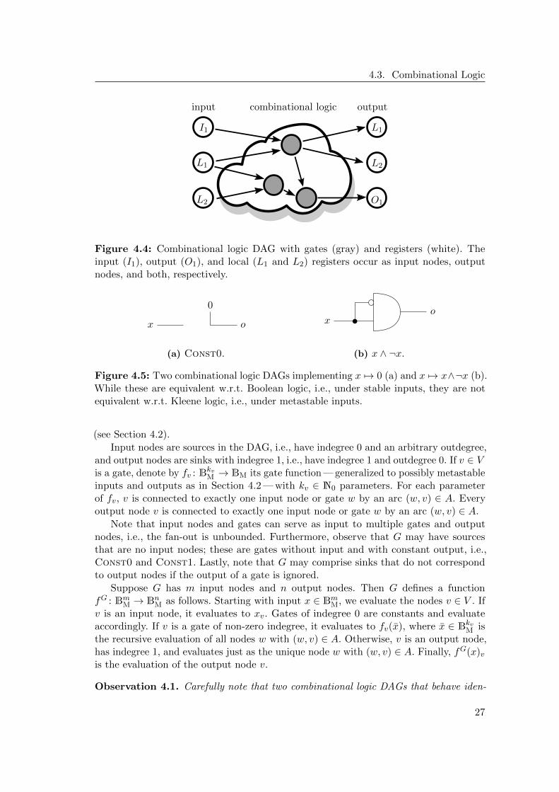
Figure 4.4: Combinational logic DAG with gates (gray) and registers (white). Theinput (I1), output (O1), and local (L1 and L2) registers occur as input nodes, outputnodes, and both, respectively.
x
0
o
(a) Const0.
xo
(b) x ∧ ¬x.
Figure 4.5: Two combinational logic DAGs implementing x 7→ 0 (a) and x 7→ x∧¬x (b).While these are equivalent w.r.t. Boolean logic, i.e., under stable inputs, they are notequivalent w.r.t. Kleene logic, i.e., under metastable inputs.
(see Section 4.2).
Input nodes are sources in the DAG, i.e., have indegree 0 and an arbitrary outdegree,and output nodes are sinks with indegree 1, i.e., have indegree 1 and outdegree 0. If v ∈ Vis a gate, denote by fv : BkvM → BM its gate function — generalized to possibly metastableinputs and outputs as in Section 4.2 — with kv ∈ N0 parameters. For each parameterof fv, v is connected to exactly one input node or gate w by an arc (w, v) ∈ A. Everyoutput node v is connected to exactly one input node or gate w by an arc (w, v) ∈ A.
Note that input nodes and gates can serve as input to multiple gates and outputnodes, i.e., the fan-out is unbounded. Furthermore, observe that G may have sourcesthat are no input nodes; these are gates without input and with constant output, i.e.,Const0 and Const1. Lastly, note that G may comprise sinks that do not correspondto output nodes if the output of a gate is ignored.
Suppose G has m input nodes and n output nodes. Then G defines a functionfG : BmM → BnM as follows. Starting with input x ∈ BmM, we evaluate the nodes v ∈ V . Ifv is an input node, it evaluates to xv. Gates of indegree 0 are constants and evaluateaccordingly. If v is a gate of non-zero indegree, it evaluates to fv(x), where x ∈ BkvM isthe recursive evaluation of all nodes w with (w, v) ∈ A. Otherwise, v is an output node,has indegree 1, and evaluates just as the unique node w with (w, v) ∈ A. Finally, fG(x)vis the evaluation of the output node v.
Observation 4.1. Carefully note that two combinational logic DAGs that behave iden-
27

Chapter 4. Circuit Model
tically under stable inputs may show different behavior in the presence of metastability.This is, in fact, a major point about containing metastability. As an example considerDAGs G and H with one input and one output node in Figure 4.5. G in Figure 4.5(a)ignores the input and always outputs 0 using a Const0 gate. The DAG H, see Fig-ure 4.5(b), uses a Not and an And gate to output x ∧ ¬x, where x is the input. Weobtain fG, fH : BM → BM with
fG(0) = fG(1) = 0 = fH(0) = fH(1). (4.7)
However, we havefG(M) = 0 6= M = fH(M). (4.8)
For a more relevant example refer to the CMUXes in Chapter 6, in particular to Fig-ure 6.2.
We proceed with a fundamental lemma about the behavior of combinational logicDAGs. Provided with a partially metastable input x, some gates — those where thecollective metastable input ports have an impact on the output — evaluate to M. Sowhen stabilizing x bit by bit, no new metastability is introduced at the gates. Furthermore,once a gate stabilized, its output is fixed; further stabilizing the input does not lead todestabilizing the output. Formally, we obtain the following lemma.
Lemma 4.2. Let G be a combinational logic DAG with m input nodes. Then for allx ∈ BmM,
x′ ∈ ResM(x) ⇒ fG(x′) ∈ ResM(fG(x)
). (4.9)
Proof. We show the statement by induction on |V |. For the sake of the proof we extendfG to all nodes of G = (V,A), i.e., write fG(x)v for the evaluation of v ∈ V w.r.t. input x,regardless of whether v is an output node. The claim is trivial for |V | = 0. Hence, supposethe claim holds for DAGs with up to i ∈ N0 vertices, and consider a DAG G = (V,A)with |V | = i+1. As G is non-empty, it contains a sink v ∈ V . Removing v allows applyingthe induction hypothesis to the remaining graph, proving that fG(x′)w ∈ ResM(fG(x)w)for all nodes w 6= v.
Concerning v, the claim is immediate if v is a source, because fG(x)v = xv if v isan input node and fG(x)v = b for a constant b ∈ BM if v is a gate of indegree 0. If v isan output node, it evaluates to the same value as the unique node w with (w, v) ∈ A,which behaves as claimed by the induction hypothesis. Otherwise v is a gate of non-zeroindegree; consider the nodes w ∈ V with (w, v) ∈ A. For input x, v receives input x ∈ BkvM ,whose components are given by fG(x)w; define x′ analogously w.r.t. input x′. By theinduction hypothesis, we have x′ ∈ ResM(x). If fv(x) = M, the claim holds becauseResM(M) = BM. On the other hand, for the case that fv(x) = b 6= M, our gate definitionentails that fv(x
′) = b, because x′ ∈ ResM(x).
Note that the evaluation of the combinational logic is entirely deterministic in ourmodel. In the physical world, however, the amplification of digital gates may “stabilize”a deteriorated input signal. This would lead to a partial stabilization of the output ofthe combinational logic DAG by an argument analogous to the proof of Lemma 4.2. Aspermitting the non-deterministic resolution of metastability during the evaluation ofthe combinational logic is equivalent to resolving it afterwards, we do the latter; this
28

4.4. Circuits
is captured in the write phase defined in Section 4.5. This simplifies the analysis whilebeing computationally equivalent to allowing partial stabilization during the evaluation.
In order to describe circuits that comprise only combinational logic and to alsocapture — possibly inconsistent — stabilization within the combinational logic, we definecombinational circuits below. We analyze them in Chapter 7. In particular, we formalizeand prove the claim that they are equivalent to combinational logic.
4.4 Circuits
With registers, gates, and combinational logic — see Sections 4.1–4.3 — at our disposal,we proceed with a formal circuit definition. We specify how it behaves in Section 4.5 andgive an example in Section 4.6.
Definition 4.3 (Circuit). A circuit C is defined by:
(1) m input registers, k local registers, and n output registers, where m, k, n ∈ N0.Each register has exactly one type — simple, mask-0, or mask-1 (see Section 4.1) —and is either input, output, or local register.
(2) A combinational logic DAG G as defined in Section 4.3. G has m+ k input nodes,exactly one for each non-output register, and k + n output nodes, exactly one foreach non-input register. Local registers appear as both input node and output node.
(3) An initialization x0 ∈ Bk+nM of the non-input registers.
Each s ∈ Bm+k+nM defines a state of C. We refer to C as simple if it only uses simple
registers and as combinational if it has no local registers.
A meaningful application clearly uses a stable initialization x0 ∈ Bk+n; this restric-tion, however, is not formally required. Furthermore, the initialization of the outputregisters is irrelevant because output registers are never read, see Section 4.5.
Combinational circuits are circuits that do not carry a state from one round into thenext. In circuit design, a combinational circuit comprises only combinational logic, butno registers; our definition, however, only requires the absence of local registers. Thisremoves the feedback loop from Figure 4.1(a). Carefully note that the required input andoutput registers are just an artifact of our definition, the “registers” of a combinationalcircuit can be interpreted as input and output pins. We analyze combinational circuitsand show that they are equivalent to our definition of combinational logic in Chapter 7.
Observe that Definition 4.3 does not allow registers to be input and output registersat the same time, an overlap in responsibilities that is often used in digital circuits. Note,however, that we impose this restriction for purely technical reasons; our model supportsregisters that are read and written — local registers — and it is possible to emulate theabovementioned behavior.3 Hence, this formal restriction has no practical implications.
3In the first round, copy the input into local registers. Use the local registers in the role where theyare both read and written in every round. Where needed, copy the content of the local registers to outputregisters in every round.
29

Chapter 4. Circuit Model
We denote by
In: Bm+k+nM → BmM, (4.10)
Loc: Bm+k+nM → BkM, and (4.11)
Out: Bm+k+nM → BnM (4.12)
the projections of circuit state to its values at input, local, and output registers, respec-tively. We use the convention that for any circuit state s, s = In(s) Loc(s) Out(s).
4.5 Executions
Consider a circuit C in state s and let x = In(s) Loc(s) be the state of the non-outputregisters. Suppose each register R is read, i.e., makes a non-dashed state transitionaccording to its type, state, and corresponding state machine in Figures 4.2(d)–4.2(f).This state transition yields a value read from, as well as a new state for, R. In general,this is a non-deterministic process as the state machines of the masking registers arenon-deterministic. We denote by
ReadC : Bm+kM → P
(Bm+k
M
)(4.13)
the function mapping x to the set of all possible values read from non-output registersof C depending on x. When only simple registers are involved, the read operation isdeterministic:
Observation 4.4. In a simple circuit C, ReadC(x) = x.Proof. By Figure 4.2(d), each simple register in state x ∈ BM has output x.
In the presence of masking registers, x ∈ ReadC(x) can occur, but the output maypartially stabilize:
Observation 4.5. Consider a circuit C in state s. Then for x = In(s) Loc(s)
x ∈ ReadC(x) and (4.14)
ReadC(x) ⊆ ResM(x). (4.15)
Proof. Check the state transitions in Figures 4.2(e) and 4.2(f). For Equation (4.14),observe that for all state machines and all states b ∈ BM a state transition with outputb ∈ BM starts in state b. Regarding (4.15), observe that registers in state M are notrestricted by the claim and registers of any type in state b ∈ B are deterministically readas b ∈ ResM(b) = b.
Let G be the combinational logic DAG of C with m+k input and k+n output nodes.Suppose o ∈ Bm+k
M is read from the non-output registers. Then the combinational logicof C evaluates to fG(o), uniquely determined by G and o. We denote all possible resultsof first reading the registers of C w.r.t. x and then evaluating the result by EvalC(x):
EvalC : Bm+kM → P
(Bk+n
M
), (4.16)
EvalC(x) :=fG(o) | o ∈ ReadC(x)
. (4.17)
30

4.5. Executions
When registers are written, we allow, but do not require, signals to stabilize. If thecombinational logic evaluates the new values for the non-input registers to x ∈ Bk+n
M ,their new state is in ResM(x); the input registers are never overwritten. We denote thisby
WriteC : Bm+kM → P
(Bk+n
M
), (4.18)
WriteC(x) :=⋃
x∈EvalC(x)
ResM(x). (4.19)
Observe that this is where metastability can cause inconsistencies: If a gate is read as Mand this is copied to three registers, it is possible that one stabilizes to 0, one to 1, and oneremains M. This is an important property of modeling metastability. Furthermore, recallfrom Section 4.3 that permitting stabilization at this point is computationally equivalentto allowing — possibly inconsistent — partial stabilization during the evaluation of thecombinational logic DAG.
For the sake of presentation, we write ReadC(s), EvalC(s), and WriteC(s) for a circuitstate s ∈ Bm+k+n
M , meaning that the irrelevant part of s is ignored.
Let sr be a state of C. A successor state sr+1 of sr is any state that can be obtainedfrom sr as follows.
Read phase First read all registers, resulting in read values o ∈ ReadC(sr). Denote byιr+1 ∈ BmM the state of the input registers after the state transitions leading toreading o.
Evaluation phase Then evaluate the combinational logic according to the result of theread phase to xr+1 = fG(o) ∈ EvalC(sr).
Write phase Pick a partial resolution xr+1 ∈ ResM(xr+1) ⊆ WriteC(sr) of the resultof the evaluation phase. Observe that the possible choices for xr+1 depend on theread phase. The successor state is sr+1 = ιr+1 xr+1.
In each clock cycle, our model determines some successor state of the current state ofthe circuit; we refer to this as round.
Note that due to worst-case propagation of metastability, the evaluation phase isdeterministic, while read and write phase are not: Non-determinism in the read phaseis required to model the non-deterministic read behavior of masking registers, and non-determinism in the write phase allows copies of metastable bits to stabilize inconsistently.In a physical circuit, metastability may resolve within the combinational logic; as arguedin Section 4.3, however, we do not model this as a non-deterministic evaluation phase,as it is equivalent to postpone possible stabilization to the write phase.
Let C be a circuit in state s0. For r ∈ N0, an r-round execution (w.r.t. s0) of C is asequence of successor states s0, s1, . . . , sr. We denote by SCr (s0) the set of possible statesresulting from r-round executions w.r.t. s0 of C:
SC0 (s0) := s0 and (4.20)
SCr (s0) :=sr | sr is a successor state of some s ∈ SCr−1(s0)
. (4.21)
31

Chapter 4. Circuit Model
I1I2
L1
L1
O1
(a) The Circuit.
rstate sr read o eval xr+1 write xr+1
I1 I2 L1 O1 I1 I2 L1 L1 O1 L1 O1
0 M M 1 1 0 M 1 M M 1 M1 M M 1 M M M 1 M M M M2 1 M M M 1 M M 1 M 1 03 1 M 1 0 1 M 1 1 1 1 14 1 M 1 1
(b) States, reads, evaluations, and writes.
Figure 4.6: Example execution in a circuit (a). The node states as well as the results ofthe read, evaluation, and write phases are listed in the table (b). Register I1 is a mask-0register, all others are simple registers. The initialization is 11, the input is MM, andhence s0 = MM11.
The initial state of C w.r.t. input ι ∈ BmM is s0 = ι x0. We use Cr : BmM → P(BnM) as afunction mapping an input of C to all possible outputs resulting from r-round executionsof C:
Cr(ι) :=
Out(sr) | sr ∈ SCr (ι x0). (4.22)
We say that r rounds of C implement f : BmM → P(BnM) if and only if Cr(ι) ⊆ f(ι) for allι ∈ BmM, i.e., if all r-round executions of C result in an output permitted by f . If thereis some r ∈ N, such that r rounds of C implement f , we say that C implements f .
Observe that our model behaves exactly like a traditional, deterministic, binary circuitmodel if s0 ∈ Bm+k+n.
4.6 Example
We use this section to present an example of our model. Figure 4.6 specifies a circuitand its states, as well as the results of the read, evaluation, and write phases. Thecombinational logic DAG implements fG(x) = (x1 ∨ x2, (x1 ∨ x2) ∧ x3). The inputregisters are I1 and I2, the only local register is L1, and the only output register is O1.Regarding register types, the input register I1 is a mask-0 register and all other registersare simple registers.
The initialization is x0 = 11, the input is ι = MM, and the initial state hence iss0 = ι x0 = MM11, which is indicated in the upper left entry in Figure 4.6(b). Inthe read phase, all non-output registers are read. Since I2 and L1 are simple registers,their read deterministically evaluates to M and 1, respectively, by the state machine inFigure 4.2(d). The mask-0 register I1 in state M may either be read as 0 and remain
32

4.7. Basic Properties
in state M, or be read as M and transition to state 1, compare Figure 4.2(e); in thiscase it does the former. So far, we fixed the outcome of the read phase, 0M1, and thefollow-up state of the input registers, MM; the other registers are overwritten at the endof the write phase. The evaluation is uniquely determined, a read phase resulting in oevaluates to fG(o), here, fG(0M1) = MM. We are left with only one more step in thisround: The non-input registers are overwritten with some value in the resolution of theevaluation phase’s result, in our case with 1M ∈ ResM(MM). Together we obtain thesuccessor state s1 = MM1M.
In the next round, I1 follows the other state transition, i.e., is read as M, and hencehas state 1 in the next round. Its state thus remains fixed in all successive rounds by thestate machine in Figure 4.2(e). The other reads are deterministic, so we obtain o = MM1as the result of the read phase and successor states 1M for I1 and I2. The evaluation isfG(o) = fG(MM1) = MM and the state of L1 and O1 is overwritten with some valuefrom ResM(MM), here, by MM.
By round r = 2, the result of the read phase is deterministic because the onlymasking register stabilized, we read o = 1MM, and evaluate to 1M. The remainingnon-determinism is whether to write 1M or some stabilization thereof; we examine thecase that 10 is written.
Rounds r ≥ 3 now are entirely deterministic. The only possible read is 1M1, whichevaluates to fG(1M1) = 11, fixing the result of the write phase to 11. Further roundsare identical: The only metastable register, I2, remains metastable but has no impact onthe evaluation phase as the Or gate always receives input 1 from I2 and hence masksthe metastable input.
4.7 Basic Properties
In this section, we establish basic properties regarding computability in the model pro-posed above. Regarding the implementability of functions by circuits, we focus on threeresources: the number r ∈ N of rounds, the register types available to it, and whetherthe circuit is combinational.
Definition 4.6 (FunrM , FunrS , and FunrC). Let FunrM be the class of functions implement-able with r rounds of arbitrary circuits. Analogously, FunrS denotes the class of functionsimplementable with r rounds in simple circuits, i.e., by circuits that may only use simpleregisters. With FunrC , we refer to the class of functions implementable with r rounds ofa combinational circuit, i.e., by circuits without local registers.
Our first claim is that the result of the write phase, i.e., WriteC , is not influenced bythe register types the circuit C uses. Carefully note that the successor state is influencedby the register types, as it accounts for the state transitions that registers make in theread phase. The reason that WriteC does not depend on the register types is as follows.By Observations 4.4 and 4.5, simple registers in state x are deterministically read as x,and masking registers in state x either as x or as some x′ ∈ ResM(x). Hence, the use ofmasking registers might partially stabilize the input to the combinational logic which,by Lemma 4.2, partially stabilizes its output. The same stabilization, however, can alsooccur in the write phase.
33
Chapter 4. Circuit Model
Lemma 4.7. Consider a circuit C in state s. Let CS be a copy of C that only usessimple registers and x = In(s) Loc(s) the projection of s to the non-output registers.Then
WriteC(s) = WriteCS (s) = ResM(fG(x)
). (4.23)
Proof. In CS , we have ReadCS (s) = x by Observation 4.4. So EvalCS (s) = fG(x),and WriteCS (s) = ResM(fG(x)) by definition.
In C, x ∈ ReadC(s) by Observation 4.5, so ResM(fG(x)) ⊆ WriteC(s). All otherreads x′ ∈ ReadC(s) have x′ ∈ ResM(x) by Observation 4.5 and fG(x′) ∈ ResM(fG(x))by Lemma 4.2. It follows that WriteC(s) = ResM(fG(x)).
Carefully note that the write phase only affects non-input registers; input registersare never written. Hence, Lemma 4.7 does not generalize to multiple rounds: Statetransitions of input registers in the read phase affect future read phases.
In 1-round executions, however, masking and simple registers are equally powerful,because their state transitions only affect rounds r ≥ 2. We show in Chapter 8 that thesestate changes may indeed lead to differences for r ≥ 2 rounds if C contains maskingregisters.
Corollary 4.8. Fun1C = Fun1
S = Fun1M .
In contrast, simple and masking registers used as non-input registers behave iden-tically, regardless of the number of rounds: A circuit C in state sr overwrites themregardless of their state. Since WriteC(sr) is oblivious to register types by Lemma 4.7,so is Loc(sr+1) Out(sr+1) for a successor state sr+1 of sr.
Corollary 4.9. Simple and masking registers are interchangeable when used as non-inputregisters.
Consider a circuit C in state s and suppose x ∈ ReadC(s) is read. Since the evaluationphase is deterministic, the evaluation y = fG(x) ∈ EvalC(s) is uniquely determined byx and C. Recall that we may resolve metastability to ResM(y) ⊆WriteC(s) in the writephase: The state of an output register R becomes 0 if yR = 0, 1 if yR = 1, and someb ∈ BM if yR = M. Consequently, output registers resolve independently:
Corollary 4.10. Let C be a circuit. Then the output bits of C after one round resolveindependently, i.e.,
C1 = g0 × · · · × gn−1, (4.24)
where gi : BmM → 0, 1,BM.
Proof. Let s = ι x0 be the initial state of C w.r.t. input ι and x = In(s) Loc(s). ByLemma 4.7, WriteC(s) = ResM(fG(x)), i.e., C1(ι) = Out(s′) | s′ ∈ ResM(fG(x)). Bydefinition, ResM(fG(x)) =
∏i∈[n] ResM(fG(x))i. Hence, the claim follows with gi(ι) :=
ResM(fG(ι Loc(x0)))i for all ι ∈ BmM and i ∈ [n].
We show in Chapter 9 that Corollary 4.10 generalizes to multiple rounds of simple cir-cuits. This is, however, not the case in the presence of masking registers, as demonstratedin Chapter 8.
Lemmas 4.2 and 4.7 apply to the input of circuits: Partially stabilizing an inputpartially stabilizes the possible inputs of the combinational logic, and hence its evaluationand the circuit’s output after one round.
34

4.8. The Next Steps
Observation 4.11. For a circuit C and input ι ∈ BmM,
ι′ ∈ ResM(ι)⇒ C1(ι′) ⊆ C1(ι). (4.25)
Proof. Let x0 be the initialization of C, s = ι x0 its initial state w.r.t. input ι, andx = In(s) Loc(s) the state of the non-output registers; define s′ and x′ equivalentlyw.r.t. input ι′ ∈ ResM(ι). Using Lemmas 4.2 and 4.7 and that ResM(x′) ⊆ ResM(x) forx′ ∈ ResM(x), we obtain that
WriteC(s′)(4.23)
= ResM(fG(x′))(4.9)
⊆ ResM(fG(x))(4.23)
= WriteC(s). (4.26)
Finally, note that adding rounds of computation to non-combinational circuits cannotdecrease computational power; a circuit determining x in r rounds can be transformedinto one using r+ 1 rounds by buffering x for one round. Furthermore, allowing maskingregisters does not decrease computational power and neither does allowing local registers.
Observation 4.12. For all r ∈ N0 we have
FunrS ⊆ Funr+1S , (4.27)
FunrM ⊆ Funr+1M , (4.28)
FunrS ⊆ FunrM , and (4.29)
FunrC ⊆ FunrM . (4.30)
4.8 The Next Steps
The subtlety of metastability in digital circuits makes it challenging to properly modelit. Especially a model that is both time-discrete and value-discrete, as the one proposedabove, runs the risk of oversimplifying matters. Hence, we are obliged to address twoissues.
(1) One is the question whether the proposed model is consistent with physical circuitproperties: Is the model “too powerful” in the sense that it permits things thatare known to be impossible in physical circuits? We address this by showing inChapter 5 that Marino’s impossibility result [108] — no digital circuit can reliablyavoid, detect, or resolve metastability — holds in our model.
(2) The other question is whether the model is not “too pessimistic” and permits non-trivial positive results. We demonstrate that this is not a problem in Chapters 6and 10, where we develop CMUXes, a core component of metastability-containingcircuits, and show that all components needed for metastability-tolerant clocksynchronization in hardware are within reach.
Together with further positive results developed using this model [26, 62, 100, 128],including simulations [26, 60, 128], this strongly indicates that the proposed model isboth useful and makes meaningful predictions.
This document is arranged such that Chapter 5, which justifies the model, is orderedbefore Chapter 6, which uses it. We refer to the first sections of Chapter 6 for relevantexamples on how to use the model.
35

Chapter 4. Circuit Model
36

CHAPTER 5
Justification
The elusive nature of metastability and Marino’s impossibility result [108] raise twoconcerns about the model proposed in Chapter 4. Is is “too optimistic” to derive mean-ingful statements about the physical world? Or is it “too pessimistic” in the sense that itdoes not permit non-trivial positive results? In this chapter, we address the first concernby showing that our model reproduces Marino’s impossibility result. We answer thesecond question in Chapter 6, where we develop CMUXes, starting with the theory atthe gate-level and advancing to optimized transistor-level implementations.
Marino established that no digital circuit can reliably (1) avoid, (2) resolve, or (3) de-tect metastability [108]. It is critical that these impossibilities are reflected by any modelcomprising metastability. We show in Theorem 5.4 and Corollaries 5.5–5.6 that (1)–(3)are impossible in the model proposed in Chapter 4 as well. Note that this is aboutputting the model to the test rather than reproducing an established result.
We first verify that avoiding metastability is impossible in non-trivial1 circuits. Con-sider a circuit C that produces different outputs for inputs ι 6= ι′. The idea is to observehow the output of C behaves while transforming ι to ι′ bit by bit, always involvingintermediate metastability, i.e., switching the differing bits from 0 to M to 1 or viceversa. This can be seen as a discrete version of Marino’s argument for signals that mapcontinuous time to continuous voltage [108]. Furthermore, the bit-wise transformationof ι to ι′, enforcing a change in the output in between, has parallels to the classicalimpossibility of consensus proof of Fischer et al. [52]; our techniques, however, are quitedifferent. The following definition formalizes the step-wise manipulation of bits.
Definition 5.1 (Pivotal Sequence). Let d ∈ N0 and ` ∈ N be integers and x, x′ ∈ BdM.Then (
x(i))i∈[`+1]
, x(i) ∈ BdM, (5.1)
is a pivotal sequence from x to x′ over BdM if and only if it satisfies
(1) x(0) = x and x(`) = x′,
(2) for all i ∈ [`], x(i) and x(i+1) differ in exactly one bit, and
(3) that bit is metastable in either x(i) or x(i+1).
Consider i ∈ [`]. We call the differing bit in x(i) and x(i+1) the pivot from i to i + 1.In the context of a pivotal sequence of circuit states, we refer to the register holding thepivot as pivotal register.
1We call the circuit C non-trivial if there are inputs ι 6= ι′ and a number of rounds r ∈ N such thatCr(ι) ∩ Cr(ι′) = ∅, i.e., if r rounds of C have to produce different outputs for ι and ι′.

Chapter 5. Justification
I1I2
L1
L1
O1
(a) The Circuit.
x(i) fG(x(i))
y(j)
I1 I2 L1 O1 L1 O1 I1 I2 L1 O1
x(0) 0 0 0 0 0 0 0 0 0 0 y(0)
x(1) 0 0 M 0 0 0 0 0 0 0
x(2) 0 0 1 0 0 0 0 0 0 0
x(3) 0 M 1 0 M M 0 M 0 0 y(1)
0 M 1 0 M M 0 M M 0 y(2)
0 M 1 0 M M 0 M M M y(3)
0 M 1 0 M M 0 M M 1 y(4)
0 M 1 0 M M 0 M 1 1 y(5)
x(4) 0 1 1 0 1 1 0 1 1 1 y(6)
(b) Pivotal sequences of circuit states for x(i) := In(x(i)) Loc
(x(i)).
Figure 5.1: A circuit with input (I1 and I2), local (L1), and output (O1) registers (a),all simple, and a pivotal sequence of circuit states x(0), . . . , x(4) with the constructedpivotal sequence of successor states y(0), . . . , y(6) (b). Each step in x is reflected in are-evaluation of the combinational logic fG(x(i)), which may affect several registers ofthe successor state. To be pivotal, the sequence y accounts for these changes bit by bit.
Carefully note that we do not use pivotal sequences as temporal sequences of successorstates. The bit-wise manipulation does not happen over time, instead, we describe closelyrelated circuit states and examine the resulting 1-round executions. The generalizationto r-round executions is made in Corollary 5.3.
We begin with Lemma 5.2, which applies to a single round of computation. It statesthat initializing a circuit C with a pivotal sequence x of circuit states results in a pivotalsequence of possible successor states y. Hence, if C is non-trivial —C guarantees differentoutputs for x(0) and x(`) — some intermediate element of y must contain a metastableoutput bit. This implies that there is a 1-round execution in which an output registerof C becomes metastable. We argue about successor states rather than just the outputbecause we inductively apply Lemma 5.2 below to obtain a statement about r-roundexecutions.
A sample circuit with pivotal sequences is depicted in Figure 5.1. Observe that inthis example, the local register L1 changes its state. This does not occur in the firstround, because the initialization for local registers is fixed. It may, however, happen insuccessive rounds.
Let x be a pivotal sequence of non-output register states, i.e., over Bm+kM , and suppose
the pivotal register changes from stable to M from x(i) to x(i+1). By Observation 4.5, we
38

may construct executions where x(i) ∈ ReadC(x(i)) and x(i+1) ∈ ReadC(x(i+1)) are theresult of the respective read phases. The key insight is that due to x(i) ∈ ResM(x(i+1)),we have
WriteC(x(i))⊆WriteC
(x(i+1)
)(5.2)
because
WriteC(x(i))
(4.23)= ResM
(fG(x(i)))
(5.3)
(4.9)
⊆ ResM
(fG(x(i+1)
))(5.4)
(4.23)= WriteC
(x(i+1)
)(5.5)
by Lemmas 4.2 and 4.7. Thus, advancing the non-output bits of the initial state fromx(i) to x(i+1) destabilizes the bits that are affected by the pivot from i to i + 1; weleave all other bits unchanged. Leveraging this, we obtain a pivotal sequence of successorstates, changing the affected output bits from stable to M one by one, each the resultof a 1-round execution of C starting in state x(i+1). A reversed version of this argumentapplies when a non-output register changes from M to stable.
Observe that this process does not guarantee that x and y have the same length;some steps in x may not lead to a new successor state at all while others may requireseveral steps for y to “catch up.” Figure 5.1 contains examples for both cases.
Lemma 5.2. Let C be a circuit and(x(i))i∈[`+1]
, x(i) ∈ Bm+k+nM , (5.6)
a pivotal sequence of states of C. Then there is a pivotal sequence(y(j))j∈[`′+1]
, y(j) ∈ Bm+k+nM , (5.7)
where each y(j) is a successor state of some x(i), satisfying that y(0) and y(`′) are successorstates of x(0) and x(`), respectively.
Proof. See Figure 5.1 for an illustration of our arguments. Let G be the combinationallogic DAG of C. Starting from x(0), we inductively proceed to x(`), extending the sequencey by a suitable, possibly empty, subsequence for each step from x(i) to x(i+1), i ∈ [`].
We maintain the invariants that
(1) For all i ∈ [`+ 1], In(x(i)) Loc(x(i)) ∈ ReadC(x(i)) is the result of the read phasein all constructed executions starting in state x(i) and that
(2) For all i ∈ [`+ 1], there is a j ∈ [`′ + 1] with
Loc(y(j))Out
(y(j))
= fG(
In(x(i)) Loc
(x(i)))
, (5.8)
i.e., where no stabilization happens in the write phase of the execution resulting instate y(j). In this context, y(j) is the state corresponding to x(i). This is the case forthe state pairs x(0) and y(0), x(1) and y(0), x(2) and y(0), x(3) and y(3), and x(4) andy(6) in Figure 5.1.
39
Chapter 5. Justification
Let ι := In(x(0)) be the state of the input registers. Lemma 4.7 guarantees that wehave fG(ι Loc(x(0))) ∈WriteC(x(0)). Define
y(0) := ι′ fG(ι Loc
(x(0)
))∈ SC1
(x(0)
), (5.9)
where ι′ is the uniquely determined state of the input registers after reading ι. Byconstruction, x(0) and y(0) fulfill the invariants.
We perform the step from x(i) to x(i+1), i ∈ [`]. Let P be the pivotal register fromx(i) to x(i+1). If P is an output register, y does not change as P has no impact on thesuccessor state, trivially completing the induction step. Hence, assume that P is aninput or local register. From the previous step, or from the definition of y(0), we havean execution resulting in state y(j) for some index j, such that In(x(i)) Loc(x(i)) is theresult of the read phase and y(j) corresponds to x(i). For the next step, we keep theresult of the read phase for all registers except P fixed. Regarding all registers that donot depend on P , i.e., may attain the same states regardless of what is read from P , werule that they attain the same states as in y(j), the state corresponding to x(i).
Suppose first that x(i)P = b 6= M and x
(i+1)P = M (e.g., the step from x(2) to x(3) with
P = I2 in Figure 5.1). Consider the set of non-input registers R that depend on P , i.e.,
R :=R | fG
(x(i))R6= fG
(x(i+1)
)R
(5.10)
(R = L1, O1 in the step from x(2) to x(3) in Figure 5.1). Since x(i) ∈ ResM(x(i+1)), byLemma 4.2 fG(x(i)) ∈ ResM(fG(x(i+1))). Hence,
fG(x(i+1)
)R
= M 6= fG(x(i))R
(5.11)
for all R ∈ R.If P is an input register, we first extend y by one item that only changes yP to M and
increase j by one if that is the case (e.g., the step from y(0) to y(1) in Figure 5.1). Thenwe extend y by y(j+1), . . . , y(j+|R|) such that in each step, for one R ∈ R, we change yRfrom bR 6= M to M. This is feasible by Corollary 4.10, as the product structure of C1
implies that we can flip any written bit without affecting the others (e.g., steps y(2) andy(3) in Figure 5.1). By construction, in state y(j+|R|) the state of the non-input registersis fG(ι x(i+1)), i.e., y(j+|R|) corresponds to x(i+1) and our invariant is satisfied.
To cover the case that x(i)P = M and x
(i+1)P = b 6= M, observe that we can apply the
same reasoning by reversing the order of the constructed subsequence.As y is pivotal by construction — we change only one bit at a time and always switch
from M to stable or vice versa — this completes the proof.
We may apply Lemma 5.2 inductively: Starting with a pivotal sequence of initialstates, we obtain executions leading to a pivotal sequence of circuit states after one round,these in turn lead to two-round executions and a pivotal sequence of circuit states aftertwo rounds, and so on.
Corollary 5.3. Let C be a circuit, x0 its initialization, and(ι(i))i∈[`+1]
, ι(i) ∈ BmM, (5.12)
40

be a pivotal sequence of inputs of C. Then there is a pivotal sequence of states(y(j))j∈[`′+1]
, y(j) ∈ Bm+k+nM , (5.13)
that C can attain after r ∈ N rounds satisfying that y(0) ∈ SCr (ι(0) x0) as well asy(`′) ∈ SCr (ι(`) x0).
Proof. Inductive application of Lemma 5.2 to C and states(ι(i) x0
)i∈[`+1]
.
The following theorem concludes that any non-trivial circuit can produce metastableoutputs, i.e., that the first of Marino’s impossibility results applies to the model proposedin Chapter 4.
Theorem 5.4. Let C be a circuit with Cr(ι) ∩ Cr(ι′) = ∅ for some ι, ι′ ∈ BmM. Then Chas an r-round execution in which an output register becomes metastable.
Proof. Apply Corollary 5.3 to a pivotal sequence from ι to ι′ and C. This yields a pivotalsequence y of states that C can attain after r-round executions. Consider(
y(i))i∈[`+1]
, y(i) ∈ BnM, (5.14)
the projection of y to the output registers that skips succeeding, identical elements. SinceCr(ι) ∩ Cr(ι′) = ∅, y is a pivotal sequence that contains at least two elements. Hence,
y(i)R = M for some output register R and some i ∈ [` + 1], i.e., there is an r-round
execution in which C outputs a metastable bit, as claimed.
Marino proved that no digital circuit can reliably (1) compute a non-constant functionand guarantee non-metastable output, (2) detect whether a register is metastable, or(3) resolve metastability of the input while faithfully propagating stable input [108].Theorem 5.4 captures (1); Corollaries 5.5 and 5.6 settle (2) and (3), respectively. Thekey is that a circuit detecting or resolving metastability is non-constant and can hencebecome metastable by Theorem 5.4, defeating the purpose of detecting or resolvingmetastability in the first place.
Corollary 5.5. There exists no circuit that implements f : BM → P(BM) with
f(x) =
1 if x = M and
0 otherwise.(5.15)
Proof. Assume such a circuit C exists and implements f using r rounds. As we haveCr(0) ∩ Cr(M) = ∅, applying Theorem 5.4 to ι = 0 and ι′ = M yields that C hasan r-round execution with metastable output. This violates the specification in Equa-tion (5.15), contradicting the assumption.
Corollary 5.6. There exists no circuit that implements f : BM → P(BM) with
f(x) =
0, 1 if x = M and
x otherwise.(5.16)
41

Chapter 5. Justification
Proof. As in Corollary 5.5 with ι = 0 and ι′ = 1.
In summary, our circuit model from Chapter 4 is consistent with physical modelsof metastability. We demonstrate in Chapters 6 and 10 that it also permits non-trivialpositive results and further examine its computational power in Chapters 7–9.
42

CHAPTER 6
Metastability-Containing Multiplexers
In this chapter, we develop Metastability-Containing Multiplexers (CMUXes). The basisof our discussion are gate-level implementations, which are a good example on how to useour model because (1) they have the right level of complexity and (2) metastability-con-tainment makes a difference in MUXes in the sense that a MUX and a CMUX behavedifferently. From a broader perspective, this demonstrates that our model, especiallythe worst-case propagation of metastability, is not “too pessimistic” to permit positiveresults while Chapter 5 shows that it is not “too optimistic,” either.
As MUXes are ubiquitous in digital circuits, we also study efficient transistor-levelCMUX implementations. The idea is that a small CMUX implementation can be usedas drop-in replacement to improve existing circuits. Bund et al. ask whether such animplementation exists [26], as existing metastability-containing sorting networks heavilydepend on CMUXes [26, 100]. Our smallest CMUX implementation uses only 8 transis-tors — no more than a standard1 transistor-level MUX — and dramatically decreases thesize of the metastability-containing sorting networks of Lenzen and Medina [100] and ofBund et al. [26], saving up to 69 % and 65 % in circuit complexity, respectively.
In this chapter, we use the following convention to simplify the specification of smallcombinational circuits.
Remark 6.1 (Notation). We specify some combinational circuits, e.g., Mux-Gate inFigure 6.1(a), only by their combinational logic DAG. The circuit in terms of Defini-tions 4.3 which we mean by that is the one that (1) only uses simple input and arbitrarilyinitialized output registers,2 (2) has no local registers, and (3) uses the given combina-tional logic DAG. We only follow this convention for combinational circuits which areequivalent to the combinational logic and w.l.o.g. use a single round of computation byTheorem 7.1.
6.1 Problem Statement
Prior to discussing metastability-containing variants, let us examine a standard MUX.An (n-bit) Multiplexer (MUX) is a circuit with 2n+ 1 inputs that implements
fMUX : BM ×BnM ×BnM → BnM (6.1)
fMUX(s, a, b) :=
ResM(a) if s = 0,
ResM(b) if s = 1, and
BnM otherwise.
(6.2)
1Pass-gate MUXes need 4 transistors but are inherently vulnerable to metastability, see Section 6.3.2.2The initialization is irrelevant as the output registers do not influence the computation.

Chapter 6. Metastability-Containing Multiplexers
b
a
s
o
(a) Mux-Gate.
b
a
s
o
(b) CMux-Gate.
b
a∆
s(mask-1)
o
(c) CMux-Delay.
Figure 6.1: Gate-level MUX implementations. Mux-Gate (a) is a standard gate-level MUX and can become metastable, see Figure 6.2. CMux-Gate (b) and CMux-Delay (c) avoid this by employing additional gates and a masking register, respectively.
For the sake of presentation, we use n = 1 throughout the chapter; all presented circuitsgeneralize to higher values of n by replication. We refer to s as the select bit. In the caseof a stable select bit, a MUX determines whether to output (some stabilization of) aor b. If s is metastable, the output is unspecified. Figure 6.1(a) shows Mux-Gate, atypical gate-level implementation of a MUX.
Note that a real-world circuit typically uses an efficient transistor-level MUX insteadof a gate-level implementation like Mux-Gate. The gate level, however, is capturedby our model from Chapter 4. Furthermore, it is well-suited for demonstrating thebasic problem with standard MUXes that is also present — although harder to see — intransistor-level MUXes. We discuss this in Section 6.3.
A desirable property of a MUX is that if a = b, the output is ResM(a), regardlessof s: Being uncertain whether to select a or b should be insubstantial in this case. If,however, s = M and a = b = 1, a standard implementation like Mux-Gate can becomemetastable, compare Figure 6.2(a).
Observation 6.2. Let CMux-Gate be the circuit associated with Mux-Gate in the senseof Remark 6.1. As depicted in Figure 6.2(a), CMux-Gate can become metastable whenprovided with input s = M and a = b = 1, i.e., CMux-Gate
1 (M, 1, 1) = BM. This followsfrom observing that (s, a, b) can be read as (M, 1, 1) by Observation 4.5, evaluating thecombinational logic DAG accordingly
(¬s ∧ a) ∨ (s ∧ b) = (¬M ∧ 1) ∨ (M ∧ 1) = M ∨M = M, (6.3)
and recalling that this implies WriteCMux-Gate
(M, 1, 1) = ResM(M) = BM.
Hence, we ask for an (n-bit) Metastability-Containing Multiplexer (CMUX), an im-proved circuit that implements
fCMUX : BM ×BnM ×BnM → BnM (6.4)
fCMUX(s, a, b) :=
ResM(a) if s = 0,
ResM(b) if s = 1, and
ResM(a⊕ b) otherwise,
(6.5)
i.e., which has to output ResM(a) if a = b, even if s = M.
44

6.2. Gate-Level Implementations
metastability
b = 1
a = 1
1M
M
1M M
s = M
o = M
(a) Mux-Gate under input s = M anda = b = 1.
b = 1
a = 1
s = M1M
M
1M M
11 1
o = 1
(b) CMux-Gate under input s = Mand a = b = 1.
Figure 6.2: Gate-level MUX behavior under inputs (s, a, b) = (M, 1, 1); in this case, theoutput should be 1 regardless of the select bit s. Mux-Gate (a), however, can becomemetastable. CMux-Gate (b) fixes this using logical masking.
6.2 Gate-Level Implementations
The circuit3 CMux-Gate in Figure 6.1(b) implements fCMUX from Equation (6.5):The problematic case of s = M and a = b = 1 is handled by the third And gate whichoutputs 1, providing the ternary Or gate with a stable 1 as input, compare Figure 6.2(b).
Lemma 6.3. One round of CCMux-Gate implements fCMUX from Equation (6.5).
Proof. CCMux-Gate has no local registers and its combinational logic DAG implements
o = (¬s ∧ a) ∨ (s ∧ b) ∨ (a ∧ b). (6.6)
It is easy to verify that this implements fCMUX from Equation (6.5) for s 6= M. Hence,consider s = M in the following. If a 6= b or a = b = M, the output of CCMux-Gate is notrestricted by Equation (6.5), so consider the remaining two cases:
Case 1 In the case of a = b = 0, all clauses in Equation (6.6) are 0, leading to o = 0.
Case 2 If a = b = 1, we have a ∧ b = 1 and o = 1, regardless of the other clauses.
Together, this concludes the proof.
The price for this improvement is an additional And gate and a ternary instead ofa binary Or gate, which can be costly if a and b have a large bit width n. Lenzen andMedina allocate 28 transistors to implement CMux-Gate, 2 for the Not, 6 for eachAnd, and 8 for the ternary Or [100]. This can be improved to 20 using Nand gates andthe de Morgan equivalent of Equation (6.6),
(¬s ∧ a) ∨ (s ∧ b) ∨ (a ∧ b) = ¬(¬(¬s ∧ a) ∧ ¬(s ∧ b) ∧ ¬(a ∧ b)), (6.7)
allocating 4 and 6 transistors for a binary and a ternary Nand, respectively [60]. Still,20 transistors are well beyond the 10 or even 6 transistors — counting the 2 transistors
3In the sense of Remark 6.1.
45

Chapter 6. Metastability-Containing Multiplexers
input: s (mask-1), a, b (simple)local: s′ (simple, initialized with 0)output: o (simple, initialized with 0)
1: each round:2: s′ ← s3: o← (¬s ∧ a) ∨ (s′ ∧ b)4: end
o
bs′as
s′
Algorithm 6.1: Two-round implementation of a CMUX. The register initialization isarbitrary and the combinational logic DAG is implied by the assignments, also compareFigure 6.1(c).
for inverting s for fair comparison — for a standard and a pass-gate implementation,respectively, see Section 6.3.
One way to reduce the number of gates is to use a masking register and a secondround of computation to implement fCMUX from Equation (6.5). This is indicated byCMux-Delay in Figure 6.1(c). First, we show how to implement fCMUX using two clockcycles and then derive from it an efficient unclocked physical implementation with fewergates. The former is captured by our model and the latter is not, because the model istime-discrete.
The two-round circuit is specified by Algorithm 6.1. It defines a clocked circuit byassignments of logic expressions to registers; in fact, it uses the same combinationallogic DAG as Mux-Gate in Figure 6.1(a). The trick is to sequentially read s from amask-1 register, ensuring that at most one copy of s can be metastable, compare thestate machine in Figure 4.2(f). This guarantees that in the case of s = M and a = b = 1,one of the And-clauses is stable 1.
Lemma 6.4. Two rounds of the circuit implied by Algorithm 6.1 implement fCMUX fromEquation (6.5).
Proof. If s 6= M, we have s = s′ after round 1 and it is easy to verify that Algorithm 6.1behaves as specified by Equation (6.5). Hence, consider s = M in the remaining partof the proof. If a 6= b or a = b = M, the output is not restricted by Equation (6.5). Soconsider s = M and a = b 6= M.
If s = M and a = b = 0, we have o = (¬s ∧ 0) ∨ (s′ ∧ 0) = 0, as claimed. Theinteresting case is s = M and a = b = 1. Here we exploit that the read phases of rounds 1and 2 only have three possible outcomes by the state machine of mask-1 registers inFigure 4.2(f): The possible reads of s are 11, 1M, and M0. Hence, in round 2, the firstbit (or a stabilization of it) is stored in s′ and the second is read from s.
Case 1 If 11 is read, s = s′ = 1, yielding
o = (¬s ∧ a) ∨ (s′ ∧ b) = (¬1 ∧ 1) ∨ (1 ∧ 1) = 1. (6.8)
Case 2 If 1M is read, we have s′ = 1 and obtain
o = (¬s ∧ a) ∨ (s′ ∧ b) = (¬s ∧ 1) ∨ (1 ∧ 1) = 1. (6.9)
46

6.3. Transistor-Level Implementations
Case 3 If M0 is read, we have s = 0 which yields
o = (¬s ∧ a) ∨ (s′ ∧ b) = (¬0 ∧ 1) ∨ (s′ ∧ 1) = 1. (6.10)
As specified, the output is 1 in each case, concluding the proof.
Observe that the circuit implied by Algorithm 6.1 uses the combinational logic fromMux-Gate which is not metastability-containing, see Figure 6.1(a). Instead of fortifyingMux-Gate with additional gates — as done in CMux-Gate in Figure 6.1(b) — Algo-rithm 6.1 uses a masking register and an additional clock cycle to fulfill the specificationof a CMUX. This construction hence does not increase the transistor count the wayCMux-Gate does and scales well with increasing bit widths n of a and b, since onlythe select bit needs to be stored in a masking register.
However, a hardware implementation of Algorithm 6.1 as a clocked state machinemay be too slow for practical applications. Fortunately, Algorithm 6.1 has an optimizedunclocked realization: The serialization of assignments in Algorithm 6.1 ensured by thetwo clock cycles can also be enforced by local delay constraints instead of clock cycles,see CMux-Delay in Figure 6.1(c). With a propagation delay from s to the And gatewith non-negated input s being larger than the gate delay from s to the And gatewith negated input ¬s— and a delay difference large enough to not observe internalmetastability of the register at both And gates simultaneously — the circuit exhibits thespecified behavior. Observe that this realization cannot be directly be expressed in ourtime-discrete circuit model from Chapter 4. However, delay lines can be avoided entirelyusing the completely digital transistor-level CMUXes presented below.
6.3 Transistor-Level Implementations
In this section, we develop efficient transistor-level implementations4 of CMUXes. Asmotivated above, MUXes are ubiquitous in digital circuits and CMUXes are used inmetastability-containing sorting networks [26, 100]. We hope that our implementationsare a contribution to the practical feasibility of metastability-containing circuits.
We propose two CMUX implementations: CMux-A is a conservative implementationthat uses 10 transistors and CMux-B uses 8 transistors at the expense of a somewhatincreased peak current and a slightly deteriorated output under s = M. Not only dowe greatly improve upon the 28 transistors that Lenzen and Medina allocate for Mux-Gate [100], see above, we also have only a marginal overhead w.r.t. classical transistor-level MUX implementations of 8 transistors. We are not, however, on par with the 4transistors of a pass-gate implementation for reasons discussed below.
Refer to Section 6.4 for a demonstration of the impact of our CMUXes. Simplyusing CMux-B as a drop-in replacement in metastability-containing sorting networksof Lenzen and Medina [100] and Bund et al. [26], which both heavily rely on CMUXes,reduces the respective circuit sizes by up to two thirds.
4We present CMOS implementations.
47

Chapter 6. Metastability-Containing Multiplexers
6.3.1 Transistors and CMOS Circuits
As the model from Chapter 4 does not capture transistor-level logic, the remaining part ofthis chapter is not covered by it. In particular, we cannot give formal correctness proofs ofthe proposed circuits within our model. However, our idea of adding a third, unspecified,signal to the digital world carries over to the transistor level and Complementary Metal-Oxide-Semiconductor (CMOS) logic. We need to examine the behavior of transistorsunder unspecified input voltages.
VDD
VSS
x x
Figure 6.3: A CMOS inverter.The transistor in the top is ap-FET, the one in the bottoman n-FET. For x = 0, the p-FETcloses and the n-FET opens, re-sulting in output 1. The oppositeis the case if x = 1.
Consider the CMOS inverter in Figure 6.3 as ex-ample. A Field-Effect Transistor (FET) has three ter-minals: source, drain, and gate. There are p-FETs andn-FETs. The transistor in the top of Figure 6.3 is ap-FET, its source is connected to VDD, logical 1, andits drain to the output on the right. The transistorin the bottom is an n-FET, its source is connected toVSS, logical 0, and its drain to the output. Both tran-sistors’ gates are connected to the input on the left.When connecting p-FET and n-FET sources to VDD
and VSS, respectively, one can think of the source asthe “input,” the drain as the “output,” and the gate asa switch controlling the source–drain resistance. Thisis an oversimplification, but it suffices for our purposes.We refer to standard literature [4, 131] for details.
The n-FET in the bottom of Figure 6.3 has a neg-ligibly small source–drain resistance when its gate isconnected to logical 1 and an extremely high source–drain resistance when connected to logical 0. Thep-FET in the top behaves the other way around: Ifthe gate is connected to logical 0 (logical 1), it has alow (high) resistance.
For x = 0, the p-FET is “closed” (conductive) andthe n-FET is “open” (non-conductive), i.e., there is a
low-resistance path from the output to VDD and only one of extremely high resistanceto VSS, resulting in output x.
This illustrates a fundamental CMOS concept: The logic is designed such that forany input, exactly one of VDD and VSS is connected to the output.
Next, we apply this line of reasoning to arbitrary voltages between logical 0 and 1,i.e., M. A FET exposed to a gate input of M might not be completely switched onor off, i.e., act as an unspecified source–drain resistance; this results in an unspecifiedoutput, i.e., M. Furthermore, a FET receiving M as source input has an unspecifiedoutput as well. In particular, when applying stable voltages — logical 0 or 1, i.e., VSS
or VDD, respectively — to a transistor’s source and drain but M to its gate, it acts asan unspecified source–drain resistance. For the inverter in Figure 6.3, x = M meansthat both transistors turn into unspecified source–drain resistances, hence, the output isunspecified.
Note that our only assumption is that the behavior is unspecified in the presence
48

6.3. Transistor-Level Implementations
s
a
a
s
s
b
b
s
o
(a) Mux-T.
b
a
o
s
s
s
(b) Mux-Pass.
s s a
a b
a b
s s a
o
(c) CMux-A.
s
s
s
s
b
a
b
a
o
(d) CMux-B.
Figure 6.4: Transistor-level MUX and CMUX implementations. Mux-T (a) and Mux-Pass (b) show conventional combinational and pass-gate MUXes, respectively. Bothare vulnerable to metastability, especially Mux-Pass: s = M causes an unspecifiedpass resistance. CMux-A (c) and CMux-B (d) implement CMUXes, i.e., metastability-containing alternatives. CMux-A requires 10 transistors and has a low peak current.CMux-B saves 2 transistors, at the expense of a slightly increased peak current in thecase of s = M and a = b.
of M, which is very conservative.
6.3.2 Standard Transistor-Level Multiplexers
Mux-T in Figure 6.4(a) is a standard transistor-level MUX. Under input s = M, allconnections from VSS or VDD to the output contain a transistor with input s or s atthe gate, i.e., an unspecified resistance. Hence, the output may be deteriorated. This isreflected by the case of fixing s = M while simultaneously switching a = b from 0 to 1or vice versa [60].
A common MUX implementation is Mux-Pass, see Figure 6.4(b). Using only fourtransistors, it forwards a or b via pass gates, i.e., without direct connections to VSS or VDD.Unfortunately, pass gates have the drawback of a non-negligible pass resistance. Thismeans that they degrade the output signal, even if all inputs are stable. Hence, chains ofpass-gate MUXes should be used with caution, possibly using signal regeneration.5 Thepass-resistance problem severely intensifies in the context of metastability-containment:s = M effectively turns all transistors of Mux-Pass into unspecified resistances. Sim-ulations reveal that when fixing s = M and simultaneously switching a = b from 0 to1 or vice versa — as above —Mux-Pass performs even worse than Mux-T [60]. Weconclude that CMUX implementations based on pass gates need to regenerate the signal.
5A slightly degenerate signal can be restored by, e.g., using an inverter. This connects to VSS or VDD
and serves as an amplifier, pulling the output towards logical 0 or 1.
49

Chapter 6. Metastability-Containing Multiplexers
This requires additional transistors and surrenders the original advantage, i.e., using fewtransistors, of a pass-gate implementation. Hence, we do not use pass gates.
6.3.3 Our Circuits
We propose two transistor-level implementations of a CMUX, referred to as CMux-Aand CMux-B and depicted in Figures 6.4(c) and 6.4(d), respectively. Both implement aCMUX up to an inverted output6 bit. CMux-A is a conservative implementation thatrequires 10 transistors. CMux-B needs only 8 transistors — the same as the conventionalMux-T— but has a slightly increased peak current and produces a slightly degradedoutput signal under s = M and a = b. Note that this is a very low overhead formetastability-containment.
10 Transistors We propose CMux-A, see Figure 6.4(c), as transistor-level implemen-tation of a CMUX. It is not hard to verify that CMux-A works correctly if all inputss, a, b are logical 0 or 1, up to inversion of the output. Regarding correct operation unders = M and a = b, recall that a transistor with an unspecified input voltage produces anunspecified output voltage. For the proposed implementation, this implies that unders = M, all transistors with gate input s or s are to be treated as unspecified resistances.
For s = M and a = b = 0, there is a low-resistance path from o to VDD at thetop right of CMux-A, but only high-resistance paths from o to VSS, so o = 1 = a. Alltransistors with voltage M at the gate are bypassed and do not influence the outputvoltage. CMux-A behaves symmetrically if s = M and a = b = 1: There is a low-resistance path from o to VSS but none from o to VDD. We conclude that CMux-Aimplements a CMUX. Simulations verify the correct behavior and establish quick andclean switching behavior under the abovementioned test case, i.e., fixing s = M andsimultaneously switching a = b from logical 0 to logical 1 and vice versa [60].
8 Transistors We propose CMux-B, see Figure 6.4(d), as an alternative to CMux-A.As above, it is not hard to check that CMux-B works correctly under stable inputs: Ifall inputs s, a, b are logical 0 or 1, CMux-B outputs a if s = 0 and b if s = 1.
So consider the case s = M and a = b. Then transistors with gate input s or s actas resistors of unspecified resistance, allowing a current from VDD to VSS along the leftpath of CMux-B. This results in an increased peak current under s = M [60].
If a = b = 1 the n-FETs pull the output low while the p-FETs on the left representan unspecified resistance, which may become low enough to cause an unspecified outputlevel. This constitutes the key difference to CMux-A which logically masks this case. Toensure correct output levels, we use transistors of double width on the right branch withinputs a and b [60]. Simulations confirm that CMux-B behaves correctly under inputs = M with this tweak [60]. In the case of a = b = 0, CMux-B behaves symmetrically.
Altogether, CMux-B implements a CMUX, but has a higher peak current thanCMux-A in the presence of a metastable select bit [60].
6This is not uncommon in digital circuit design, e.g., Mux-T does the same.
50

6.4. Impact on Metastability-Containing Circuits
6.4 Impact on Metastability-Containing Circuits
In this section, we demonstrate how our CMUX implementations drastically reducethe complexity of existing metastability-containing circuits. This is achieved by simplyusing CMux-A or CMux-B as a drop-in replacement wherever a CMUX is required. Wedemonstrate this using the metastability-containing sorting networks for BRGC proposedby Lenzen and Medina [100] and the more recent improvement by Bund et al. [26]; usingCMux-B reduces the size of 16-bit sorting networks by 69 % and 65 %, respectively.
Both papers describe 2-sort implementations that work for inputs that are eitherBRGC numbers or metastable superpositions of successive BRGC numbers. As BRGConly changes one bit in an increment, the latter can only become metastable at thatparticular bit, if implemented correctly [62]. We shed some light on this in Chapter 10.
For a 2-sort of B-bit BRGC numbers, Lenzen and Medina require O(B2) transistorsand Bund et al. O(B logB). Each paper presents the transistor counts required byoptimal sorting networks of 4, 7, and 10 channels for B ∈ 2, 4, 8, 16 assembled fromtheir respective 2-sort implementation. Both papers use the abovementioned 28-transistorestimate for CMux-Gate by Lenzen and Medina [100].
a
b
c
d
ott
ss
Figure 6.5: 4-CMUX assembledfrom three 2-CMUXes [100].
The proposed 2-sort implementations requirea 4-CMUX, i.e., a CMUX that uses two selectbits to choose one of four inputs. A 4-CMUX isa straightforward generalization of fCMUX fromEquation (6.5) and can be assembled from threeCMUXes as in Figure 6.5 [100]. Note that us-ing CMux-A or CMux-B in this two-level ap-proach doubly negates the output and hence di-rectly produces the desired result. Together withfour transistors to invert both select bits, we require3 · 8 + 4 = 28 transistors to implement a 4-CMUXfrom CMux-B,7 much less than the 3·28 = 84 tran-sistors allocated in both implementations [26, 100].Note that in the 2-sort derived from Lenzen andMedina [100], we only need a total of two invertersfor each recursion level, as both 4-CMUXes use thesame select bits.
Table 6.1 shows how replacing the naive CMUXimplementation by CMux-B from Figure 6.4(d) reduces the transistor count ofmetastability-containing sorting networks and gives an overview on how large thesenetworks are.
Regarding the comparison with Lenzen and Medina, note that the authors present apolynomially as well as an exponentially sized 2-sort [100]. The exponentially sized 2-sortis more efficient for B ∈ 2, 4. We always plug CMux-B into the polynomially sizedcircuit and compare it to the unmodified polynomially sized circuit. A comparison withthe exponentially sized circuit would be obscured, because Lenzen and Medina reportinconsistent transistor counts for them: The size of a 4-, 7-, and 10-sort is not exactly 5,
7Using CMux-A requires 3 · 10 + 4 = 34 transistors.
51

Chapter 6. Metastability-Containing Multiplexers
bits4-sort 7-sort 10-sort
[100] we saved [100] we saved [100] we saved
2 540 340 37.0 % 1728 1088 37.0 % 3132 1972 37.0 %4 4020 1620 59.7 % 12864 5184 59.7 % 23316 9396 59.7 %8 21060 7060 66.5 % 67392 22592 66.5 % 122148 40948 66.5 %16 95460 29460 69.1 % 305472 94272 69.1 % 553668 170868 69.1 %
bits4-sort 7-sort 10-sort
[26] we saved [26] we saved [26] we saved
2 960 400 58.3 % 3072 1280 58.3 % 5568 2320 58.3 %4 4440 1640 63.1 % 14208 5248 63.1 % 25752 9512 63.1 %8 13920 4960 64.4 % 44544 15872 64.4 % 80736 28768 64.4 %16 37080 13000 65.0 % 118656 41600 65.0 % 215064 75400 65.0 %
Table 6.1: Transistors saved by using CMux-B in the sorting networks of Lenzen andMedina [100] and Bund et al. [26].
10, and 29 times8 that of a 2-sort. This, however, only makes a difference for B ∈ 2, 4,as the polynomially sized 2-sort is smaller for B ∈ 8, 16 and higher.
Our approach saves between 37.0 % and 69.1 % of the transistors in the describedsettings. The savings w.r.t. Bund et al. [26] are equally drastic: Using CMux-B reducesthe size of the sorting network by 58.3 %–65.0 %, removing almost two thirds of theoriginal circuit.
8The number of 2-sorts in the respective sorting networks.
52

CHAPTER 7
Combinational Circuits
In this chapter, we analyze combinational circuits. Note that in circuit design, the term“combinational circuit” refers to circuits using only combinational logic and no registers;we define combinational circuits as circuits without local registers. At first glance thismay seem different, but the concept is the same: A combinational circuit does notremember previous clock cycles. As the only feedback loop in our model leads throughthe local registers, compare Figure 4.1(a), we can establish that property by removingthem. The input and output registers required by Definition 4.3 merely are a consequenceof moving the non-determinism of possible stabilization out of the combinational logic;we discuss this in Section 4.3. Hence the “registers” of a combinational circuit can simplybe interpreted as input and output pins attached to the combinational logic.
We fully classify the functions implementable by combinational circuits and formallyshow that the output of a combinational circuit is — up to possible stabilization ofmetastable output bits — equivalent to its combinational logic. Furthermore, we showthat it does not matter which registers are used in combinational circuits, formalizingthe above claim that they may be interpreted as input and output pins.
This implies that in combinational circuits, our model essentially boils down toSections 4.2 and 4.3: gates and combinational logic. Put differently, Kleene logic modelsmetastability in combinational circuits. We consider this a strong indicator that ourmodel is quite natural. In Chapter 8, we show that simple circuits are computationallyequivalent to combinational circuits as well. The reason our model requires the additionalcomplexity of registers, clock cycles, and non-determinism is to capture masking registers;we demonstrate in Chapter 8 that circuits with masking are computationally strictlymore powerful than simple circuits.
Theorem 7.1 (Combinational Circuits). Let C be a combinational circuit with combi-national logic DAG G, m input registers, and n output registers. Then we have
C1(ι) = Cr(ι) = ResM(fG(ι)
)(7.1)
for all r ∈ N and all inputs ι ∈ BmM and hence
Fun1C = FunrC (7.2)
for all r ∈ N. Furthermore, it holds for all ι ∈ BmM and all i ∈ [n] that
C1(ι)i = 0 ⇔ fG(ι)i = 0, (7.3)
C1(ι)i = 1 ⇔ fG(ι)i = 1, and (7.4)
C1(ι)i = BM ⇔ fG(ι)i = M. (7.5)

Chapter 7. Combinational Circuits
Proof. Let ι ∈ BmM and r ∈ N be an arbitrary input and a number of rounds. In orderto show that Cr(ι) = ResM(fG(ι)), observe that there is an execution where we read ιfrom the input registers in round r by the state machines in Figures 4.2(d)–4.2(f): Eachinput register R maintains state ιR for r− 1 rounds and makes the uniquely determinedstate transition resulting in output ιR in round r. The combinational logic DAG thenevaluates to fG(ι) in the r-th evaluation phase and the possible writes are ResM(fG(ι)),showing that
Cr(ι) ⊇ ResM(fG(ι)). (7.6)
Further observe that — also by the state machines in Figures 4.2(d)–4.2(f) — the r-thread phase is guaranteed to yield some ι′ ∈ ResM(ι). Hence, the combinational logicDAG always evaluates to some fG(ι′) ∈ ResM(fG(ι)) by Lemma 4.2 and all possiblewrites are in ResM(fG(ι)). This guarantees
Cr(ι) ⊆ ResM(fG(ι)). (7.7)
As the above arguments hold for arbitrary ι and r, and in particular for r = 1, Equa-tion (7.1), and with it Equation (7.2), follows.
Claims (7.3)–(7.5) are a direct consequence of the definition of the write phase; ifthe combinational logic evaluates to x, the possible writes are ResM(x).
Note that Equation (7.1) is independent from the register types used in the com-binational circuit. This reflects the above informal statement that the registers of acombinational circuit can be interpreted as input and output pins.
Observation 7.2. Let C be a combinational circuit. Then C1 is invariant under changingthe register types used in C.
In the light of Theorem 7.1, we simplify notation to
FunC := Fun1C . (7.8)
We establish in Chapter 8 that the computational power of combinational circuitsis the same as that of simple circuits, as simple circuits can be unrolled. However,circuits that may use masking registers become strictly more powerful with each roundof computation.
54

CHAPTER 8
Computational Hierarchy
In this chapter, we determine the impact of the number of rounds, of the available registertypes, and whether local registers are permitted on the computational power of circuitsin the model from Chapter 4. Recall from Definition 4.6 that FunrM , FunrS , and FunrCdenote the functions implementable using r ∈ N rounds in arbitrary circuits, in simplecircuits, and in combinational circuits, respectively, where simple circuits are restricted tosimple registers and combinational circuits have no local registers. Further recall that thenumber of rounds is irrelevant in combinational circuits, i.e., that FunC = Fun1
C = FunrCby Theorem 7.1. The main results are the following.
(1) Even in the presence of metastability, circuits restricted to simple registers canbe unrolled. This means that r ∈ N copies of the combinational logic can bearranged to implement r rounds of the original circuit in a single round. In termsof computable functions, this means that FunS := Fun1
S = FunrS . We discuss thisin Section 8.1.
(2) Combinational circuits are exactly as powerful as simple circuits: FunC = FunS .This is discussed in Section 8.2.
(3) With masking registers, however, unrolled circuits are not equivalent to multiplerounds of computation anymore. Regarding computable functions, we show inSection 8.3 that this leads to a strict inclusion: FunrM ( Funr+1
M for all r ∈ N.
Together with Corollary 4.8, we obtain the following hierarchy:
FunC = FunS = Fun1M ( Fun2
M ( Fun3M ( · · · . (8.1)
We believe this to make a strong case for further pursuing masking registers in researchregarding metastability-containing circuits.
8.1 Simple Circuits
It is folklore that binary-valued synchronous circuits can be unrolled such that theoutput after r ∈ N clock cycles of the original circuit is equal to the output aftera single clock cycle of the unrolled circuit. Theorem 8.1 states that this result alsoholds in presence of potentially metastable simple registers. Carefully note that thisresult — defying intuition — does not carry over to circuits with masking registers, seeTheorem 8.3.
Theorem 8.1 (Unrolling). Given a simple circuit C and r ∈ N, one can construct asimple circuit C ′ such that C ′1 = Cr. In particular, if r rounds of C implement f , a singleround of C ′ implements f . Hence, it holds that
∀r ∈ N : Fun1S = FunrS . (8.2)

Chapter 8. Computational Hierarchy
I1
L1
L2
L1
L2
L1
L2
L1
L2
O1
Figure 8.1: Unrolling three rounds of the circuit in Figure 4.4 with three gates (gray),and four registers (white). Local registers (L1 and L2) become Id gates and early outputis ignored.
Proof. The claim is trivial for r = 1, hence suppose r ≥ 2. We construct a circuit C ′
with C ′1(ι) = C2(ι). Given C, we construct C ′ as follows, compare Figure 8.1. Let G bethe combinational logic DAG of C, consider two copies G1 = (V1, A1) and G2 = (V2, A2)of G, and let G′ = (V1 ∪ V2, A1 ∪A2) be the combinational logic DAG of C ′, up to thefollowing modifications.
(1) Every input register I of C corresponds to input nodes vI1 ∈ V1 and vI2 ∈ V2. IdentifyvI1 , vI2 to a single input node in G′ (compare I1 in Figure 8.1) and associate itwith a new input register in C ′; apply this to all input registers of C.
(2) In order to ignore “early” output, replace each output node in G1 correspondingto an output register in C with a gate that has one input and whose output isignored (like the first two copies of O1 in Figure 8.1).
(3) The remaining input and output nodes are associated with local registers. Eachlocal register L of C corresponds to exactly one output node vL1 ∈ V1 and one inputnode vL2 ∈ V2. Identify vL1 , vL2 to an Id gate in G′ that simply forwards its input(the center copies of L1 and L2 in Figure 8.1).
Associate the k remaining input nodes of G1 and output nodes of G2 with local registers,maintaining the original mapping. Observe that G′ has n input, m output, and k localregisters; we rule that all registers are simple. Define the initial state of C ′ as that of C.
To check that one round of C ′ is equivalent to two rounds of C, let ι ∈ BmM be an input,s0 the initial state of both C and C ′ w.r.t. input ι, and x0 = In(s0) Loc(s0) the initialstate of the non-output registers. As all registers are simple, we have ReadC
′(x0) = x0
by Observation 4.4 and hence, by construction of G′,
EvalC′(s0) =
fG′(x0)
=fG(ι Loc
(fG(x0)
)). (8.3)
In C, we have WriteC(s0) = ResM(fG(x0)) by Lemma 4.7. Recall that by the statemachine in Figure 4.2(d), simple registers do not change their state when read. Thus,
56

8.2. Combinational Circuits
when C is in some state s1 ∈ SC1 after the first round, we have that
ReadC(s1) = ι Loc(s1) (8.4)
⊆ι Loc(x) | x ∈WriteC(s0)
(8.5)
⊆ ResM(ι Loc
(fG(x0)
)), (8.6)
using Observation 4.4. By Lemma 4.2, we obtain
EvalC(s1) ⊆ ResM(fG(ι Loc
(fG(x0)
))). (8.7)
This means that the second evaluation phase of C yields a stabilization of the firstevaluation phase of C ′, because the write phase allows for arbitrary stabilization. Onthe other hand, it is possible that no stabilization happens in C, as the unstabilizedι Loc(fG(x0)) ∈ EvalC(s1). Together, we have SC2 = SC
′1 and C ′1(ι) = C2(ι) follows.
An inductive application of the above arguments yields the claims.
Naturally, the unrolled circuit is larger than the original and a physical implementationneeds longer clock cycles, as the increase in delay is linear in r. However, the point isthat adding rounds does not affect the computational power of simple circuits. In thelight of Theorem 8.1, we use
FunS := Fun1S (8.8)
in the following.
8.2 Combinational Circuits
As simple circuits can be unrolled, local registers do not contribute to their computationalpower. Hence, simple circuits are exactly as powerful as combinational circuits.
Theorem 8.2. We have
FunS = FunC . (8.9)
Proof. Consider f ∈ FunC . By Observation 7.2, there is a simple, combinational circuitC that implements f . As C is simple, f ∈ FunS and hence FunC ⊆ FunS .
On the other hand, consider f ∈ FunS . By Theorem 8.1, there is a simple circuit Cthat implements f in a single round. As C only uses one round, its local registers areonly read once. Hence, replacing each local register with a Const0 or a Const1 gate,depending on its initialization, yields a combinational circuit that implements f . Weconclude FunS ⊆ FunC and the claim follows.
8.3 Arbitrary Circuits
As discussed above, additional rounds make no difference in terms of computability forsimple and combinational circuits; the corresponding hierarchies collapse into FunS . Inthe presence of masking registers, however, unrolled circuits are not equivalent to multiplerounds of computation: As detailed in Section 8.1, unrolling requires an input registerto be connected to each copy of the combinational logic. Since a masking register in
57

Chapter 8. Computational Hierarchy
Ir−1
I2
O1
Or
O2
Ir−2
I1
...
...
1
M
1
0
O3
L1
L2
L1
L2C
Figure 8.2: Simulating a masking register with a selector.
state M may be read as M, all these copies may receive M as input. This, however, doesnot happen when reading from the masking register sequentially: A masking registerguarantees that M is read at most once, compare Figure 4.2.
Below, we demonstrate that this leads to a strict inclusion: FunrM ( Funr+1M for
all r ∈ N. We show this using a metastability-containing fan-out buffer specified byEquation (8.10). It creates r copies of its input bit, at most one of which is permittedto become metastable:
f(x) :=
xr if x 6= M and⋃i∈[r] ResM
(0iM1r−i−1
)otherwise.
(8.10)
Theorem 8.3. It holds that
∀r ∈ N : FunrM ( Funr+1M . (8.11)
Proof. Fix 2 ≤ r ∈ N and consider f from Equation (8.10). We first show f ∈ FunrM ,and then that f /∈ Funr−1
M .First observe that f is implemented by r rounds of the circuit C which uses a mask-0
input register Rr−1 and a chain of local registers Rr−2, . . . , R0. In each round, the valueread from register Ri+1, i ∈ [r − 1], is copied to Ri and output register Oi, i ∈ [r], getsthe value read from Ri. Observe that the specification of a mask-0 register is such that,given an initial state, r reads (and possibly stabilization in the write phase) may returnexactly the sequences specified in Equation (8.10). Since C faithfully copies these values,it follows that f = Cr ∈ FunrM .
Below, we show that f /∈ Funr−1M , for which we use the following subcircuits:
r-round counters take no input and have r outputs, such that the (i− 1)-th outputis 1 in round 1 ≤ i ≤ r and 0 else. This is implemented by a linear chain of localregisters Ri, i ∈ [r], where each Ri is copied to Ri+1 for i ∈ [r− 1], R0 is initializedto 1 and all others to 0. Output register Oi, i ∈ [r − 1], is fed the Xor of Riand Ri+1, and Rr−1 is copied to Or−1.
r-round selectors take r inputs xi, i ∈ [r], and have one output O, such that the stateof O in round 1 ≤ i ≤ r is in ResM(xi−1), i.e., holds a copy of xi−1. This is achieved
58

8.3. Arbitrary Circuits
using an r-round counter and feeding the And of xi and the i-th counter outputinto an r-ary Or, the output of which is written to O.
We claim that f /∈ Funr−1M . Assume for contradiction that there is a circuit C such
that r − 1 rounds of C implement f , i.e., Cr−1 ⊆ f . We derive a contradiction bysimulating the behavior of C in a circuit C ′ with r− 1 simple input registers, which mayinitially hold any possible sequence of values read from the input register of C in r − 1rounds.
By Corollary 4.9, we may assume w.l.o.g. that all non-input registers ofC are simple. Ifthe only input register of C is also simple as well, we may unroll C into C by Theorem 8.1.Applying Lemma 4.7 to C yields Mr ∈ C1(M) = Cr−1(M) /∈ f(M), i.e., violating thespecification. Hence, suppose the input register of C is a masking register.
Consider the case that the input register is a mask-0 register and compare Figure 8.2.Define C ′ as a copy of C, except that r − 1 simple input registers serve as input to an(r − 1)-round selector. This compound represents the only input register R of C: Everygate or output node driven by R in C is instead connected to the selector’s output in C ′.
A surjective mapping of executions of C ′ with inputs restricted to all possible se-quences of r − 1 reads from R in state M, i.e., restricted to inputs
0r−1∪
0iM1r−i−2 | i ∈ [r − 1], (8.12)
to executions of C is defined as follows. We interpret the selector’s output in round r asthe value read from R in round r and “copy” the remaining execution of C ′ (withoutinputs and the selector) to obtain a complete execution of C. As our restriction of theinputs reflects exactly the possible reads of a mask-0 register, see the state machine inFigure 4.2(e), the result always is a feasible execution of C with input M.
By Theorem 8.1, we may w.l.o.g. assume that a single round of C ′ implements f .Consider the sequence of C ′-inputs from 0r−1 to 1r−1 in which we flip the bits one byone from right to left, from 0 to 1, with some parallels to Fischer et al. [52]. By thepigeon hole principle, there must be some 1 ≤ r ≤ r − 1 so that two output bits of C ′
change compared to r − 1. Since, when fixing the other input bits, two outputs ` 6= `′
depend on the r-th input bit from the right and C ′ only uses simple registers, we haveby Lemma 4.7 that
MM ∈WriteC′ (
0r−r−1M1r−1 x0
)`,`′
, (8.13)
where x0 is the initialization of the local registers. Hence, ` and `′ can become metastablein the same execution of C ′. We map this execution to an execution of C, in which thecorresponding output registers attain the same state (i.e., two of them are M) afterr− 1 rounds. This contradicts the assumption that r− 1 rounds of C implement f fromEquation (8.10).
The above argument covers the case that the input register is a mask-0 register. Amask-1 register is handled analogously by replacing Equation (8.12) with all possiblereads of a mask-1 register, i.e., by
1r−1∪
1iM0r−i−2 | i ∈ [r − 1], (8.14)
and adapting the subsequent arguments accordingly.
59

Chapter 8. Computational Hierarchy
From the contradictions derived above, we conclude that Cr−1 6⊆ f . This impliesthat f /∈ Funr−1
M and Funr−1M 6= FunrM . As r ≥ 2 was arbitrary and, by Observation 4.12,
Funr−1M ⊆ FunrM , this concludes the proof.
60

CHAPTER 9
Simple and Combinational Circuits
In this chapter, we fully classify FunS = FunC . By Theorems 8.1 and 8.2, our resultscarry over to an arbitrary number of rounds in simple circuits and to combinationalcircuits in particular. We present sufficient and necessary conditions for a function to beimplementable with a simple or combinational circuit.
Using this classification, we demonstrate how to take an arbitrary Boolean functionf : Bm → Bn and extend it to the most restrictive specification [f ]M : BmM → P(BnM),the metastable closure of f , that is implementable in simple and combinational circuits.
The way to use this when designing metastability-containing circuits is to start with afunction f required as component, “lift” it to [f ]M, and check whether [f ]M is restrictiveenough for the application at hand. If it is, one can work on an efficient implementationof [f ]M, otherwise a new strategy, possibly involving masking registers, must be devised.
9.1 Natural Subfunctions
Let C be a simple circuit. From Corollary 4.10 and Observation 4.11, we know that C1,the set of possible circuit outputs after a single round, has three properties: (1) its outputcan be specified bit-wise, (2) each output bit is either 0, 1, or completely unspecified,and (3) stabilizing a partially metastable input restricts the set of possible outputs.Hence C1 — and by Theorems 8.1 and 8.2 all simple and combinational circuits — can berepresented in terms of bit-wise Karnaugh maps with values “0, 1,BM” instead of“0, 1, D” (D for “don’t care”); as this is equivalent to combinational logic by Theorem 7.1,we may also use “0, 1,M.” We call such functions natural and show below that f ∈ FunSif and only if f has a natural subfunction.
Definition 9.1 (Natural Function). The function f : BmM → P(BnM) is natural if andonly if it is bit-wise, closed, and specific:
Bit-wise The components f1, . . . , fn of f are independent:
f(x) = f1(x)× · · · × fn(x). (9.1)
Closed Each component of f is specified as either 0, as 1, or completely unspecified:
∀x ∈ BmM : f(x) ∈ 0, 1,BMn . (9.2)
Specific Stabilizing partially metastable input does not destabilize the output of f :
∀x ∈ BmM : x′ ∈ Res(x)⇒ f(x′) ⊆ f(x). (9.3)

Chapter 9. Simple and Combinational Circuits
Suppose we ask whether a function f is implementable with a simple or combinationalcircuit, i.e., if f ∈ FunS . If there is a simple circuit that implements f , we can unrollit by Theorem 8.1 and may thus assume w.l.o.g. that C1 ⊆ f . Hence, Corollary 4.10and Observation 4.11 state a necessary condition for f ∈ FunS : f must have a naturalsubfunction. Theorem 9.2 establishes that this condition is sufficient, too.
The main technique of Theorem 9.2 — covering all prime implicants — is mentionedby Huffman [74] and formally shown to prevent logic hazards by Eichelberger [43], whoalso uses Kleene logic [90]. This is owed to the fact that Eichelberger uses Kleene logicto model gate behavior under switching inputs [43]. As what we refer to as “M” includesarbitrary signal behavior over time — see Chapter 4 — and hence also switching signals,this analogy is not surprising. For the sake of self-containment and as our notation andmodel are quite different, we state and prove Theorem 9.2.
Theorem 9.2. Let g : BmM → P(BnM) be a function. Then it holds that g ∈ FunS if andonly if g has a natural subfunction.
Proof. Regarding the “⇒” direction, we have a simple circuit C such that C1 ⊆ g byTheorem 8.1. C1 is bit-wise and closed by Corollary 4.10 and specific by Observation 4.11.Hence, C1 is a natural subfunction of g.
We proceed with the “⇐” direction. Let f ⊆ g be a natural subfunction of g; weconstruct a circuit C that implements f in one round. As f is bit-wise, we may w.l.o.g.assume that n = 1. If f = const0 or f = constBM
, let C be the circuit whose outputregister is driven by a Const0 gate; if f = const1, use a Const1 gate.
Otherwise, consider fB : Bm → 0, 1 given by
fB(x) =
0 if f(x) = 0 or f(x) = BM and
1 if f(x) = 1.(9.4)
We call a partial variable assignment A that implies fB(x) = 1 for all x obeying Aan implicant of fB; if the number of variables fixed by A is minimal w.r.t. A being animplicant, we refer to A as a prime implicant of fB [29].
Construct the combinational logic DAG of C in a Disjunctive Normal Form (DNF)fashion: Use an And gate1 for each prime implicant of fB, with inputs connected to therespective, possibly negated, input registers. The respective outputs feed an Or gate2
driving the circuit’s only output register. See Figure 9.1 for an illustration. C has minput registers, no local registers, and one output register; all registers are simple asrequired. The initialization of the output register is arbitrary. By construction, we havethat
∀x ∈ Bm : C1(x) = fB(x) ⊆ f(x). (9.5)
To see that C1 ⊆ f , consider x ∈ BmM \Bm and make a case distinction.
Case 1 If f(x) = BM, then trivially C1(x) ⊆ f(x).
1If no And gate of sufficient fan-in is available, use a tree of And gates. For the sake of presentation,and because it is equivalent to the tree, we assume an And gate of sufficient fan-in is available.
2As above, we assume an Or gate of sufficient fan-in is available.
62

9.1. Natural Subfunctions
ab
s
00 01 11 10
0
1
11
1 1
0 0
0 0
Figure 9.1: Karnaugh map of a MUX. Mux-Gate from Chapter 6 covers the primeimplicants sa = 01 and sb = 11. The metastability-containing implementation CMux-Gate additionally covers ab = 11; this corresponds to the construction in the proof ofTheorem 9.2.
Case 2 If f(x) = 0, we have for all x′ ∈ Res(x) that f(x′) = 0 = fB(x′) byEquation (9.3), as f is specific. Thus, for each such x′, all And gates, correspondingto prime implicants, output 0. Furthermore, under input x and for each And gate,there must be at least one input that is stable 0: Otherwise, there would be somex′ ∈ Res(x) making one And gate, i.e., prime implicant, output 1, resulting inC1(x′) = 1 and contradicting Equation (9.5). By our definition of gate behavior,this entails that all And gates output 0 for all x′ ∈ ResM(x) as well, and hence
C1(x) = 0 = f(x). (9.6)
Case 3 If f(x) = 1, all x′ ∈ Res(x) have f(x′) = fB(x′) = 1 by Equation (9.3).Thus, fB outputs 1 independently from the metastable bits in x, and there is aprime implicant of fB which relies only on stable bits in x. By construction, someAnd gate in C implements that prime implicant. This And gate receives onlystable inputs from x, and hence outputs a stable 1. The Or gate receives that 1as input and, by definition of gate behavior, outputs stable 1. We conclude that
C1(x) = 1 = f(x). (9.7)
As f is closed, the above case distinction is exhaustive. The claim follows as one roundof C implements f .
As an example, consider a binary single-bit MUX specification f : B3 → B,
f(s, a, b) =
a if s = 0 and
b otherwise,(9.8)
and its Karnaugh map in Figure 9.1. A DNF implementation that is unaware of metasta-bility only has to cover all ones in the Karnaugh map with implicants. This is achievedby implementing the prime implicants sa = 01 and sb = 11, which is exactly what Mux-Gate from Chapter 6 does. Applying the construction of the proof of Theorem 9.2, on
63

Chapter 9. Simple and Combinational Circuits
the other hand, requires implementing all prime implicants, i.e., to implement ab = 11in addition to sa = 01 and sb = 11. This yields CMux-Gate from Chapter 6, a CMUXimplementation.
9.2 Metastable Closure
Consider a Boolean function f : Bm → Bn. Lift the definition of f to [f ]M : BmM → P(BnM),dealing with metastable inputs analogously to gate behavior in Section 4.2: Whenever allmetastable input bits together can influence the output, specify the output as “anythingin BM.” We call [f ]M the metastable closure of f , and argue below that [f ]M ∈ FunS . Forf : BmM → P(BnM), i.e., for more flexible specifications, [f ]M is defined analogously. Notethat the concept of the metastable closure is equivalent to the absence of Eichelberger’slogic hazards [43].
Definition 9.3 (Metastable Closure). For a function f : BmM → P(BnM), we define itsmetastable closure [f ]M : BmM → P(BnM) component-wise for i ∈ [n] by
[f ]M(x)i :=
0 if ∀x′ ∈ ResM(x) : f(x′)i = 0,1 if ∀x′ ∈ ResM(x) : f(x′)i = 1, and
BM otherwise.
(9.9)
We generalize this to Boolean functions. For f : Bm → Bn, we define [f ]M : BmM → P(BnM)as
[f ]M(x)i :=
0 if ∀x′ ∈ Res(x) : f(x′)i = 0,
1 if ∀x′ ∈ Res(x) : f(x′)i = 1, and
BM otherwise.
(9.10)
Example 9.4. The metastable closure of a binary MUX specification from Equation (9.8)is exactly the specification of a CMUX from Equation (6.5).
Observe that Equation (9.10) is equivalent to the behavior we demand from gatesin Section 4.2 when identifying 0 with 0, 1 with 1, and M with BM, respectively.Furthermore, note that for f : Bm → Bn, the metastable closure is very closely relatedto the metastable superposition:
[f ]M(x) = ResM
⊕x′∈Res(x)
f(x′) . (9.11)
Most importantly, observe that [f ]M is bit-wise, closed, and specific by construction;hence [f ]M is natural.
Observation 9.5. [f ]M ∈ FunS for all f : Bm → Bn and all f : BmM → P(BnM).
An immediate consequence of Observation 9.5, Theorem 8.1, and Theorem 8.2 forthe construction of circuits is that, given an arbitrary Boolean function f : Bm → Bn,there are simple and combinational circuits that implement [f ]M in a single round.
64

9.3. Open Problem
Observation 9.6. For f : Bm → Bn, Theorem 9.2 shows that [f ]M is the most restrictiveextension of f implementable with simple or combinational circuits: By Equation (9.3),any natural extension g of f must satisfy
∀x ∈ BmM, ∀i ∈ [n] :⋃
x′∈Res(x)
f(x′)i ⊆ g(x)i, (9.12)
and thus that
∃x′, x′′ ∈ Res(x) : f(x′)i 6= f(x′′)i ⇒ g(x)i = BM (9.13)
by Equation (9.2).
In order to show that a function is not implementable with simple registers only, itsuffices to show that it violates the preconditions of Theorem 9.2, i.e., that it has nonatural subfunction.
Example 9.7. Consider f : B2M → P(B2
M) with
f(x) := ResM(x) \ MM. (9.14)
This function specifies to copy a 2-bit input; if there is metastability in the input, it may bepropagated to at most one output. This specification does not contradict the impossibilityresults discussed in Chapter 5, but still, no circuit without masking registers implements f ,i.e., f /∈ FunS.
Proof. Assume for the sake of contradiction that f ∈ FunS , i.e., that f has a naturalsubfunction g ⊆ f by Theorem 9.2.
As specified in Equation (9.14), f(00)1 = 0 and f(11)1 = 1. Since g ⊆ f andg(x) 6= ∅ because g is closed, we have g(00)1 = 0 and g(11)1 = 1. The fact that gis specific implies that g(00)1 ∪ g(11)1 ⊆ g(MM)1, i.e., 0, 1 ∈ g(MM)1. This in turnmeans that g(MM)1 = BM, because g is closed. Furthermore, we know that g is bit-wise,so g = g1 × g2 with g1(00) = 0, g1(11) = 1, and g1(MM) = BM. Analogously,g2(00) = 0, g2(11) = 1, and g2(MM) = BM.
Since g is bit-wise, g(MM) = g1(MM) × g2(MM) 3 MM, but MM /∈ f(MM),contradicting the assumption g ⊆ f . As we did not make any restrictions regarding g,this holds for all natural subfunctions of f . It follows that f /∈ FunS .
9.3 Open Problem
Theorem 9.2 is useful for checking if a combinational or simple circuit implementing somefunction exists. Furthermore, its proof is constructive, providing an indication on whereto start with the design of such a circuit. However, it is well-known that covering allprime implicants can be costly as there may be exponentially many [29]. While efficientmetastability-containing implementations for some problems are known [26, 100], thereis a fundamental open question: What is the overhead of implementing the metastableclosure?
65

Chapter 9. Simple and Combinational Circuits
More precisely, let f : Bm → Bn be a Boolean function and consider the smallestpossible combinational circuit, in terms of the number of gates, that implements
f : BmM → P (BnM) (9.15)
f(x) =
f(x) if x ∈ Bm and
BM otherwise.(9.16)
What is the worst-case overhead of implementing [f ]M instead of f in a combinationalcircuit w.r.t. a fixed set of gates?
As an example, the combinational circuits Mux-Gate and CMux-Gate in Chap-ter 6 which implement fMUX and fCMUX = [fMUX]M, respectively. When restrictingthe gate fan-in to 2, CMux-Gate uses six gates3 and Mux-Gate only uses four4 butdoes not implement [fMUX]M. Is there a gate-level CMUX with five or four gates whenrestricted to Const0, Const1, Not, binary Or, and binary And?
3CMux-Gate uses one Not, three And, and two Or gates.4Mux-Gate has one Not, two And, and one Or gate.
66

CHAPTER 10
Clock Synchronization
We establish the implementability of the fault-tolerant clock-synchronization algorithmby Lundelius Welch and Lynch [106] with a deterministic correctness guarantee, despitethe unavoidable [108] presence of metastable upsets. As we do not require synchronizers,yet tolerate metastable upsets, this has two important consequences:
(1) Synchronization delay does not impose a fundamental limit on the operating fre-quency of clock-synchronization algorithms in hardware.
(2) An implementation of the proposed algorithm can, in principle, remove the risk ofmetastability from communication across clock domains altogether, as communi-cation between synchronized clock domains does not incur metastable upsets.
We demonstrate that a variety of metastability-containing combinational circuits —referred to as components — can be implemented. Due to the machinery established inthe preceding chapters, this is possible with simple checks, usually using Observation 9.5.We remark that since the paper this chapter is based on [55] appeared, efficient imple-mentations of some of the components described below have been proposed [26, 62, 100].The list of components we present is by no means an exhaustive list on what compu-tations can be realized in a metastability-containing way, yet it permits implementinga highly non-trivial application: a hardware implementation of the fault-tolerant clocksynchronization algorithm of Lundelius Welch and Lynch [106].
The algorithm of Lundelius Welch and Lynch is widely applied, e.g., in the Time-Triggered Protocol (TTP) [92, 93, 94] — in the context of the TTP, this is commonlyreferred to as the fault-tolerant average algorithm, which uses the strategy of Lun-delius Welch and Lynch, see Kopetz and Ochsenreiter [94] — and FlexRay [17] clock-synchronization protocols. Kopetz et al. predict an achievable precision in the orderof microseconds for software–hardware based implementations of TTP [93]. High oper-ating frequencies, however, ultimately require a pure hardware implementation: 1 GHzclocks, for example, only leave very few CPU cycles per pulse. Kinali et al. presentan FPGA implementation that uses synchronizers instead of metastability-containingtechniques [83]. We are not aware of a metastability-containing implementation of theclock-synchronization algorithm as a whole.
All known implementations synchronize potentially metastable inputs from the TDCsbefore computations. This technique becomes less reliable with increasing operatingfrequencies since less time is available for metastability resolution. Furthermore, lowtemperatures and supply voltages intensify this issue [14]. Moreover, classical bounds forthe MTBF regarding metastable upsets in synchronizers assume a uniform distributionof input transitions [13, 89]; this is not guaranteed to be the case in clock synchronization,since the goal is to align clock ticks. Either way, synchronizers merely increase the odds
Chapter 10. Clock Synchronization
of stabilization and we prefer deterministic correctness guarantees over a probabilisticstatement.
In order to demonstrate why, recall that the MTBF is estimated by Equation (3.2).Suppose, we want to synchronize 1 GHz clocks, this yields FC = FD = 109 Hz. Thevalues τ and TW depend on the technology; SPICE [127] simulations for an ASIC usinga 130 nm process yield τ = 31.6 · 10−12 s and TW = 8 · 10−12 s [62]. Assuming that 50 %,80 %, and 100 % of the clock cycle are available for stabilization yields MTBF estimationsof
MTBF0.5 ns ≈e15.823
8 · 106s ≈ 0.9 s, (10.1)
MTBF0.8 ns ≈e25.316
8 · 106s ≈ 12.3 · 103 s (3.5 hours), and (10.2)
MTBF1.0 ns ≈e31.646
8 · 106s ≈ 6.9 · 106 s (80 days). (10.3)
This means that the MTBF drops to less than a second per synchronizer when reservinghalf the clock cycle for stabilization, rises to about 3.5 hours for the more conservativeestimate of 0.8 ns, but never exceeds approximately 80 days, even when leaving no timefor computations. Note that these estimates are per synchronizer of which n(n− 1) areneeded, where n ≥ 4 is required in order to tolerate one fault.
The MTBF is catastrophic for a synchronization delay of 0.8 ns and does not permitthe implementation of a mission-critical system, even for a synchronization delay of 1 ns.Hence, we are left with two options. One is to include pipelining in the algorithm ofLundelius Welch and Lynch such that it reacts to measurements only after a sufficientsynchronization delay. This means that the difference between clocks indicated by ameasurement may grow during the synchronization delay reserved for stabilization ofthat measurement, hence pipelining reduces the quality of clock synchronization. Thealternative is to develop a metastability-containing implementation; we propose one inthe following.
Also observe that allotting time t for using synchronizers before beginning the com-putation imposes a fundamental limit of 1/t on the operating frequency. In the light ofever-increasing operating frequencies, we ask: Does the unavoidable presence of meta-stable upsets when measuring relative timing deviations pose a principal limit on theoperating frequency? Below, we argue that this is not the case. We demonstrate thefeasibility of a hardware implementation of the Lundelius Welch and Lynch algorithmthat does not depend on metastability-free inputs and thus does not suffer from systemfailures induced by metastable upsets.
10.1 Algorithm
The algorithm of Lundelius Welch and Lynch works on n fully connected nodes with alocal clock each [106]. Each node generates clock pulses, measures their difference to theother nodes’ clock pulses, and adjusts its local clock accordingly. The algorithm toleratesup to f < n/3 Byzantine [96] faults.
Our core strategy is a separation of concerns, compare Figure 3.1, between the analogand the digital part of the circuit:
68

10.1. Algorithm
remote start
D Q
E
D Q
E
D Q
E
D Q
E
D Q
E
local stop
Figure 10.1: Tapped delay line TDC. It is read as either 1k0n−k or 1kM0n−k−1, i.e.,produces at most one metastable bit and hence has precision-1.
(1) The arrival times of incoming analog clock pulses relative to a node’s internal clockare measured using TDCs,
(2) metastability-containing components ensure that the digital part of the circuit han-dles the potentially partially metastable outcome of the time-to-digital conversion,and
(3) the digital, possibly still partially metastable, signals are converted to analog signalscontrolling the local clock.
This process provides a guaranteed end-to-end uncertainty of a single bit throughout alldigital computations, see below, without the hazard of spreading metastability in thecontrol logic in an uncontrolled fashion. Given Marino’s result [108], we find it highlysurprising that such a thing is possible. The key is that the digital part of the circuitcan become metastable, but that metastability is properly contained and ultimatelytranslated into bounded fluctuations in the analog world, not contradicting Marino.
Sophisticated implementations of individual components introduced below have beenproposed [26, 62, 100] since the result this chapter is based on [55] first appeared; wepoint them out below.
We propose a hardware implementation in which each node does the following.
Step 1: Analog to Digital First, we step from the analog into the digital world:Delays between remote pulses and the local pulse are measured with TDCs. The mea-surement can be realized such that at most one of the output bits, accounting for thedifference between x and x + 1 ticks, becomes metastable; we say such numbers haveprecision-1 and formally define them in Section 10.2.
TDCs can be implemented using tapped delay lines [69, 122, 123], see Figure 10.1: Aline of delay elements is tapped in between each two consecutive elements, driving thedata input port of initially enabled latches initialized to 0. The rising transition of theremote clock signal fed into the delay line’s input passes through the line and sequentiallysets the latches to 1; the rising transition of the local clock signal is used to disable alllatches at once. After that, the delay line’s latches contain the time difference as unaryTC. Choosing the propagation delays between the latches larger than their setup/holdtimes, we ensure that at most one bit is metastable, i.e., that their status is of the form1∗0∗ or 1∗M0∗. The output is hence a precision-1 TC-encoded time difference.
The recently proposed metastability-containing TDC by Fugger et al., building uponour ideas, implements this step and the next [62].
69
Chapter 10. Clock Synchronization
Step 2: Encoding We translate the time differences into BRGC, making storageand subsequent components much more efficient. The results are BRGC-encoded timedifferences with at most one metastable bit of precision-1.
In this step, metastability-containing TC to BRGC conversion is needed and wediscuss it in Section 10.3. A more efficient way is to use a metastability-containing TDCwhich directly produces BRGC of precision-1. As stated above, building on our ideas,such a component has recently been proposed by Fugger et al. [62].
Step 3: Sorting Network A sorting network selects the (f + 1)-th and (n − f)-thlargest remote-to-local clock differences; tolerating f faults requires discarding the topand bottom f values [106].
This requires 2-sort building blocks that pick the minimum and maximum of twoprecision-1 BRGC-encoded inputs preserving precision-1. We discuss this in Section 10.3;recently, efficient implementations based on our techniques have been presented by Lenzenand Medina [100] and Bund et al. [26], which we improve in Chapter 6.
Step 4: Decoding and Digital to Analog The BRGC-encoded (f + 1)-th and(n − f)-th largest remote-to-local clock differences are translated back to TC-encodednumbers. As discussed in Section 10.3, this can be done preserving precision-1, i.e., suchthat the results are of the form 1∗0∗ or 1∗M0∗.
This can be used to we step back into the analog world, again without losing precision:The two values are used to control the local clock frequency via a Digitally ControlledOscillator (DCO). However, the DCO design must be chosen with care. Designs thatswitch between inverter chains of different length to modify the frequency of a ringoscillator cannot be used, as metastable switches may occur exactly when a pulse passes.Instead, we propose using a ring oscillator whose frequency is controlled by effects suchas digitally controlled current sources, capacitor banks, and resistances [39]. While the atmost two metastable control bits — at most one in each remote-to-local clock difference —may dynamically change the load of two inverters, this has a limited effect on the overallfrequency change and does not lead to glitches within the ring oscillator, because theeffect on the clock speed is in the convex hull of the effects of all stabilizations of thedigital control parameters.
10.2 Encoding and Precision
An appropriate encoding is key to designing metastability-containing components.
Example 10.1 (Binary). Suppose a control bit u indicating whether to increase x = 7 by1 is metastable and x is encoded in standard binary. The result must be some resolutionof the metastable superposition, see Equation (4.4), of 00111 and 01000, i.e., anythingin Res(00111 ⊕ 01000) = Res(0MMMM) and thus any number x′ ∈ [16], even afterstabilization.
The original uncertainty between 7 and 8 is massively amplified; a good encodingshould allow to contain the uncertainty imposed by u = M.
70

10.3. Digital Components
A code is an injective function γ : [n]→ Bk mapping a natural number x ∈ [n] to itsencoded representation. For y = γ(x), we define γ−1(y) := x, and for sets X,
γ(X) := γ(x) | x ∈ X and (10.4)
γ−1(X) := x | γ(x) ∈ X. (10.5)
We need two encodings: Thermometer Code (TC) and Binary Reflected Gray Code(BRGC). For the k-bit (unary) TC we use
un: [k + 1]→ Bk (10.6)
un(x) := 0k−x1x. (10.7)
BRGC, compare Figure 10.2(a), is represented by rg(x) and is much more efficient, usingonly dlog2 ne bits. In fact, rg : [2k] → Bk is bijective. We choose un and rg due to theproperty that in both encodings γ(x) and γ(x+1) differ in a single bit only. This rendersthem suitable for metastability-containing operations.
Example 10.2 (TC and BRGC). We revisit Example 10.1 with the metastable controlbit u indicating whether to increase x = 7 by 1.
TC In 9-bit TC, 7 is encoded as 001111111 and 8 as 011111111, so their metastablesuperposition resolves to Res(0M1111111), i.e., only to un(7) or un(8). Unaryencoding, however, is very inefficient regarding the number of bits.
BRGC Analogously, in 5-bit BRGC, 7 is encoded as 00100 and 8 as 01100, compareFigure 10.2(a), so their metastable superposition resolves to Res(0M100), i.e., onlyto rg(7) or rg(8).
Since the original uncertainty is whether or not to increase x = 7 by 1, the uncertaintyis perfectly contained instead of amplified as with binary code in Example 10.1.
We formalize the notion of the amount of uncertainty in a partially metastable codeword: x ∈ BkM has precision-p (w.r.t. the code γ) if
maxy − y | y, y ∈ γ−1(Res(x))
≤ p, (10.8)
i.e., if the largest possible difference between resolutions of x is bounded by p.Note that the components presented below make heavy use of BRGC. This makes
them more involved, but they are exponentially more efficient than their TC coun-terparts in terms of memory and avoid the amplification of uncertainties incurred bystandard binary encoding. As a matter of fact, recently proposed efficient implementa-tions for metastability-containing sorting networks [26, 100] and metastability-containingTDCs [62] use BRGC.
10.3 Digital Components
In the following, we show that all metastability-containing components required for theclock synchronization algorithm outlined in Section 10.1 exist. As motivated above, thecomponents have to maintain meaningful outputs in face of limited metastability; moreprecisely, we deal with the abovementioned precision-1 output of TDCs.
71

Chapter 10. Clock Synchronization
dec O1 O2 O3
0 0 0 01 0 0 12 0 1 13 0 1 04 1 1 05 1 1 16 1 0 17 1 0 0
(a) 3-bit BRGC.
O1I4
O2I2
I6I2
I6
O3
I1
I3
I5
I7
I1
I3
I5
I7
(b) Transformation circuit.
Figure 10.2: Efficient TC-to-BRGC conversion.
TC-to-BRGC Converter Figure 10.2(b) depicts a circuit that translates 7-bit TCinto 3-bit BRGC. It generalizes to n-bit inputs, with a depth of dlog2 ne. While suchtranslation circuits are well-known, it is important to check that the given circuit fulfillsthe required property of preserving precision-1: This holds as each input bit influencesexactly one output bit and, due to the structure of BRGC, this bit makes exactly thedifference between rg(x) and rg(x+ 1) given a TC-encoded input of 1xM07−x−1.
Sorting Networks It is well-known that sorting networks can be efficiently composedfrom 2-sort building blocks [3, 11], which map (x, y) to (minx, y,maxx, y). We showthat max (and analogously min) of two precision-1 k-bit BRGC numbers is implementablewith combinational logic, i.e., without masking registers, such that each output hasprecision-1. Observe that this is straightforward for TC-encoded inputs with bit-wiseAnd and Or for min and max, respectively. However, this is possible for BRGC inputsas well.
Lemma 10.3. Define maxBRGC : Bk ×Bk → Bk as
maxBRGC(x, y) := rg(max
rg−1(x), rg−1(y)
). (10.9)
Then [maxBRGC]M ∈ FunS and it determines precision-1 output from precision-1 inputsx and y.
Proof. Since x and y have precision-1, rg−1(Res(x)) ⊆ a, a+ 1 for some a ∈ [2k − 1](analogously for y w.r.t. some b ∈ [2k − 1]). W.l.o.g. assume a ≥ b, i.e., for all possibleresolutions of x and y, the circuit must output rg(a) or rg(a+ 1). By Definition 9.3 andthe fact that rg(a) and rg(a+ 1) differ in a single bit only, [maxBRGC]M(x, y) has at mostone metastable bit and precision-1.
An analogous argument holds for
minBRGC(x, y) := rg(min
rg−1(x), rg−1(y)
). (10.10)
Observe that sorting precision-1 BRGC numbers may lead to the following effect:Consider rg(6)⊕ rg(7) = 10M, the metastable superposition of 6 and 7 in 3-bit BRGC,
72
10.3. Digital Components
compare Figure 10.2(a). Then
[maxBRGC]M (10M, 10M) = ResM(10M) = [minBRGC]M (10M, 10M). (10.11)
Hence, it is possible that after stabilization 100 = rg(7) is ordered before 101 = rg(6). Bydefinition of the metastable closure and due to using precision-1 BRGC input, however,the flipped order can only occur between numbers that differ by at most 1, i.e., the erroris bounded by the initial uncertainty.
Based on our proposed 2-sort building blocks, Lenzen and Medina [100] and Bundet al. [26] present implementations using O(k2) and O(k log k) gates, respectively.
Metastability-containing sorting networks open up another option. If we insist onusing synchronizers, we can still deploy them after sorting and selecting the (f + 1)-thand (n− f)-th largest remote-to-local clock differences. While this does not remove thesynchronization delay, it reduces the total number of synchronizers from n(n− 1) to 2n,i.e., from O(n2) to O(n). This trade-off, however, may only become interesting for largevalues of n and low-overhead precision-1 BRGC comparators.
BRGC-to-TC Converter A BRGC-encoded number of precision-1 has at most onemetastable bit: For any up-count from an encoding of x ∈ [2k − 1] to x+ 1 a single bitchanges, which thus can become metastable if it has precision-1. It is possible to preservethis guarantee when converting to TC.
Lemma 10.4. Define rg2un: Bk → B(2k−1) as
rg2un(x) := un(rg−1(x)
). (10.12)
Then [rg2un]M ∈ FunS converts its parameter to TC, preserving precision-1.
Proof. If x has precision-1, then rg−1(Res(x)) ⊆ a, a+ 1 for some a ∈ [2k − 1]. Hence,un(a) and un(a+ 1) differ exactly in the (a+ 1)-th bit, proving the claim.
73

Chapter 10. Clock Synchronization
74

CHAPTER 11
Conclusion
No digital circuit can reliably avoid, detect, or resolve metastable upsets [108]. Whilethe standard approach is to use synchronizers to trade time for an increased MTBF [13,14, 15, 67, 88, 89], we propose a fundamentally different method: It is possible to designefficient digital circuits that tolerate a certain degree of metastability in the input. Thistechnique has critical advantages:
(1) Where synchronizers decrease the odds of failure, our techniques provide deter-ministic guarantees. A synchronizer may or may not stabilize in the allotted timeframe. Our model, on the other hand, guarantees to return one of a specific set ofknown values — e.g., the metastable closure, but this depends on the application —without relying on probabilities.
(2) Our approach saves time and, by eliminating synchronizers, removes one funda-mental limitation on the operating frequency. If the required functions can beimplemented in a metastability-containing way, there is no need to reserve timefor synchronization before starting the computation.
(3) If metastability needs to be resolved eventually, one can still save time by allowingfor stabilization during the metastability-containing computations.
In light of these properties, we expect our techniques to prove useful for a variety ofapplications, in particular in time- and mission-critical scenarios.
Our argumentation is based on a model developed in Chapter 4. It captures clockedand combinational circuits and models the spread of metastability in a worst-case fashion.In the absence of metastability, it behaves like a regular circuit model. We check themerits of our model by showing in Chapter 5 that it reproduces the known impossibilityof avoiding, detecting, or resolving metastability. Further, we demonstrate in Chapter 6that the explanatory power of our model extends to the transistor level by developingCMOS implementations of CMUXes.
We show in Chapters 7 and 8 that circuits with simple registers can be unrolledand are computationally equivalent to combinational circuits. In this case, our modelcan be simplified to Kleene logic in combinational logic DAGs, making reasoning aboutcircuits much more convenient than in the general case. The presence of masking regis-ters, however, strictly increases the computational power with each clock cycle; we areable to establish a strict inclusion result. Furthermore, we fully classify all functionsimplementable in combinational and simple circuits in Chapter 9.
As a consequence of our techniques, we establish the implementability of the fault-tolerant clock synchronization algorithm by Lundelius Welch and Lynch [106] witha deterministic correctness guarantee, despite the unavoidable presence of metastableupsets, in Chapter 10.

Chapter 11. Conclusion
Recent Developments A range of promising results has been obtained based on ourwork: metastability-containing sorting networks [26, 100], a TDC that directly producesprecision-1 BRGC [62], and metastability-aware network-on-chip routers [128]. Togetherwith verification in simulations [26, 60, 128], we believe this to strengthen the case forthe explanatory power of our model.
Future Work We focus on computability under metastable inputs. There are manyopen questions regarding circuit complexity in our model of computation.
It is of interest to reduce the gate complexity and latency of concrete circuits, aswell as to determine the complexity overhead of metastability-containment in general.In particular, the overhead of implementing the metastable closure [f ]M as comparedto an implementation of f that is oblivious to metastability — and if there has to be anoverhead at all — is an open question, in general as well as for particular functions f , seeSection 9.3.
Masking registers are computationally strictly more powerful than simple registers(Theorem 8.3). An open question is which metastability-containing circuits benefit frommasking registers and to find further examples separating FunrM from Funr+1
M .Our model does not capture clock gating, i.e., non-input registers are overwritten in
every clock cycle. Hence, storing intermediate results in masking registers is pointless:Taking advantage of at most one read from an input masking-register becoming meta-stable does not apply to results of intermediate computations. It is an open problemwhether this makes a difference in terms of computability.
76

PART II
Parallel Distance Problems
“Confusion is the only thing that grows when shared.”
A confused meerkat
This part is the result of close collaboration with Christoph Lenzen. Thetext is based on an article that is under submission to the Journal of theACM (JACM) as of August 2016, an extended abstract of which appeared inthe Proceedings of the 28th ACM Symposium on Parallelism in Algorithmsand Architectures (SPAA 2016), pages 455–466, 2016 [61].

78
CHAPTER 12
Introduction
Many problems in computer science are intrinsically linked to distances in graphs. Thiscertainly is due to the fact that graphs are an extremely useful tool for modeling re-lationships between discrete entities. Hence, it is not surprising that some of the mostclassic algorithms determine distances in graphs, e.g., Dijkstra’s algorithm [41] and theMoore-Bellman-Ford (MBF) algorithm [16, 54, 116]. But distance problems are by nomeans a closed book; recent literature offers plenty of results on this front. We cannothope to give an exhaustive list of related work, but would like to mention distanceapproximations [20, 34, 48, 73, 91, 101, 103, 135], spanners [10], hop sets [34, 48, 73],algebraic distance computations [5, 35, 115, 135], metric tree embeddings [6, 8, 9, 20, 21,50, 65, 81, 110], and distributed algorithms [10, 65, 73, 81, 101, 102, 103, 104, 107, 119].
Another highly relevant topic are parallel computations [10, 19, 21, 22, 33, 34, 48,77, 91, 105, 107, 113]. Gigantic data centers, the distributed storage and processing ofinformation, and large-scale computer networks are commonplace. Given the relevanceof graph problems and that they grow more and more complex, it is highly relevant toharness the power of parallel machines in this context, as pointed out by, e.g., Lumsdaineet al. [105].
Our goal are polylogarithmic depth (parallel time) algorithms of little work (totalnumber of operations). The work can be thought of as the time required by a sequentialmachine and the depth as a lower bound on the time required by a parallel machine withan arbitrary number of processors and without synchronization overhead. Ideally, analgorithm’s work is close to the time of a fast sequential algorithm for the same problem.
We study parallel computations of distance problems in graphs; our focus are distanceapproximations that preserve the triangle inequality. To see the relevance in this, letG = (V,E, ω) be a graph with n vertices and m edges and recall that exact distancesin G, denoted by dist(·, ·, G) : V × V → R≥0 ∪ ∞,1 fulfill the triangle inequality:
∀u, v, w ∈ V : dist(u,w,G) ≤ dist(u, v,G) + dist(v, w,G), (12.1)
i.e., the “direct route” from u to w is never heavier than any “detour” visiting u, v, andw in order. The triangle inequality is one of the properties required from a metric.
Exact distances automatically fulfill the triangle inequality. In order to obtain efficientparallel algorithms, however, we often resort to approximate distances. The problem isthat if d : V ×V → R≥0∪∞ is an α-approximation of dist(·, ·, G), the triangle inequalitydoes not necessarily hold in d. This is irrelevant for some problems — e.g., finding anapproximately shortest path between two vertices — but it is highly relevant for others.As an example, the probabilistic metric tree embedding of Fakcharoenphol, Rao, andTalwar (FRT) relies on the subtractive form of the triangle inequality [50].
1Below, we use the notation introduced in Section 12.3 without explicit forward references.
Chapter 12. Introduction
Hence, we study approximate, parallel, polylogarithmic-depth, work-efficient algo-rithms that either explicitly compute or implicitly work on approximate metrics, i.e.,obey the triangle inequality. We list our contributions below, however, one key result arealgorithms that w.h.p. determine a (1+o(1))- and O(1)-approximate metric of dist(·, ·, G)using polylog n depth and O(n(m+n1+ε)) and O(n2+ε) work, respectively. Observe thatthe latter is close to the trivial lower bound of Ω(n2) work for writing the result. Anotherkey result is that we can w.h.p. sample a probabilistic FRT-style tree embedding of Gthat has an expected stretch of O(log n) using polylog n depth and O(m1+ε) work. Thework can be reduced to O(m+ n1+ε) at the expense of increasing the expected stretchto O(ε−1 log n). In both cases, the work is close to O(m log n), the state of the art in thesequential setting [20].
MBF-like Algorithms In order to obtain algorithms that use polylogarithmic depthwhile at the same time being work-efficient and guaranteeing consistency with the triangleinequality, we resort to a virtual graph H. It has a Shortest-Path Diameter (SPD) ofO(log2 n), meaning that we can find shortest paths with at most SPD(H) ∈ O(log2 n)hops between each pair of nodes. This resolves the issue with the triangle inequality —we compute exact distances in H which automatically form a metric — and maintainsthe possibility of polylogarithmic depth, as O(log2 n) iterations suffice. Assuming wemay add an appropriate hop set [34] to G, dist(·, ·, H) is a (1 + o(1))-approximation ofdist(·, ·, G), meaning that the computed distances are essentially as good as those in G.
Unfortunately, H is a complete graph. Hence, explicitly computing the adjacencylists of H, or even performing a single iteration in H, incurs Ω(n2) work; this defeatsthe hope of near-linear work in the number of edges of G.
Fortunately, we can simulate the iterations of an algorithm in H using iterationsin G and polylogarithmic overhead in both work and depth. The simulation requiressome structural properties of the algorithm, but generally works for algorithms that“behave like the MBF algorithm.” We formalize this notion, propose the class of Moore-Bellman-Ford-like (MBF-like) algorithms, and show that the simulation argument holdsfor them.
Our classification of MBF-like algorithms provides a new perspective on a clas-sical scheme of spreading information through a graph that is a key ingredient tomany algorithms [16, 54, 65, 73, 81, 101, 102, 103, 104, 116]. Further, it captures awide range of known algorithms, including but not limited to source detection, Single-Source Shortest Paths (SSSP), k-Source Shortest Paths (k-SSP), All-Pairs ShortestPaths (APSP) and Multi-Source Shortest Paths (MSSP) over the min-plus semiring,Single-Source Widest Paths (SSWP), All-Pairs Widest Paths (APWP) and Multi-SourceWidest Paths (MSWP) over the max-min semiring, the more involved k-Shortest Dis-tance Problem (k-SDP) and k-Distinct-Shortest Distance Problem (k-DSDP) over theall-paths semiring, and connectivity over the Boolean semiring. As the above list is byno means complete, we conclude that our classification is rather flexible and consider itof independent interest.
The basic observation is that in an MBF-like algorithm each node in each iteration(1) propagates the information obtained so far to all its neighbors, (2) then aggregatesthe received information, and (3) optionally filters out irrelevant parts. As an example,consider k-SSP, where we determine, for each node, the k nodes closest to it. Each node
80

stores node–distance pairs (initially only themselves at distance 0) and then iteratesthe following steps: (1) propagate the node–distance pairs to the neighbors, uniformlyincreasing distances by the corresponding edge weight, (2) aggregate the received valuesby picking the minimum distance for each node, and (3) discard node–distance pairs forwhich there are k closer alternatives.
An MBF-like algorithm has three key components: a semiring S, a semimoduleM = (M,⊕,) over S, and a filter r : M→M. The semiring captures how distancesand edge weights interact in the underlying graph. A standard choice is the min-plussemiring that is a common tool for distance problems [5, 35, 115, 135]. We use thesemimoduleM as a “data structure” for collecting information that can be accumulatedduring the algorithm. M might be a single distance when solving SSSP or a vector of ndistances for APSP. Propagation corresponds to and aggregation to ⊕.
The filter is a projection that discards information which is irrelevant for the algorithmat hand. Roughly speaking, in an h-iteration MBF-like algorithm, each node determinesits part of the output based on its h-hop distances to all other nodes. For efficiencyreasons, however, various algorithms [65, 73, 81, 101, 102, 103, 104, 115] compute onlya subset of these distances. The role of the filter is to remove the irrelevant values toallow for better efficiency. The core feature of an MBF-like algorithm is that filteringis “compatible” with propagation and aggregation: If a node discards information andthen propagates it, the discarded parts must be “uninteresting” at the receiving node aswell. We model this using a congruence relation on the node states; filters pick a suitable(efficiently encodable) representative of the node state’s equivalence class.
We hope that relatively few standard choices for S and M can be reused for manyalgorithms, leaving it up to the filter to implement the algorithm-specific customization.Hence, we hope that the framework of MBF-like algorithms, besides capturing manyalgorithms, easily extends to further algorithms. This is different from Mohri’s frameworkwhich requires a custom semiring for each algorithm [115].
Our Approach APSP and MSSP determine a metric and a submetric, respectively,and collecting Least Element (LE) lists [33] readily allows to sample an FRT tree [21, 81],the abovementioned tree embedding of expected logarithmic stretch. These algorithmsare MBF-like, hence we may simulate them in H to obtain good approximations of whatthese algorithms would determine in G. Observe that running any of these algorithmsin G to determine exact distances — in order to respect the triangle inequality — takesSPD(G) iterations, where SPD(G) = n− 1 is possible. This corresponds to linear depthand hence is not an option in our setting. We sample an FRT tree (alternatively, determinea metric or a submetric) using the following sequence of embeddings. Starting with thegraph G, we
(1) first obtain G′ by adding a (d, ε)-hop set, where d, ε−1 ∈ polylog n to G [34], then
(2) metrically embed G′ into H (implicitly), and
(3) embed H into an FRT tree (alternatively, determine a metric or submetric).
Is the second step required, i.e., is there no hop-set algorithm that ensures that d-hopdistances satisfy the triangle inequality? Unfortunately, hop sets do not solve the problem.
81

Chapter 12. Introduction
First recall that a (d, ε)-hop set is a set of edges that, when added to the graph, ensuresthat d-hop distances in G′ approximate dist(·, ·, G), i.e., ensure that
∀v, w ∈ V : dist(v, w,G) ≤ distd(v, w,G′) ≤ (1 + ε) dist(v, w,G), (12.2)
where G′ is G augmented with the hop-set edges [34]. Put differently, hop sets guaranteethat d-hop distances approximate distances. However, any hop set that fulfills the triangleinequality on d-hop distances has to reduce the SPD to at most d, i.e., yield exactdistances, which is a much harder problem:
Observation 12.1. Let G be a graph that contains a (d, ε)-hop set. If distd(·, ·, G) is ametric, then distd(·, ·, G) = dist(·, ·, G), i.e., SPD(G) ≤ d.
Proof. Let π be a shortest u-v-path in G. Since distd(·, ·, G) fulfills the triangle inequality,
distd(u, v,G) ≤∑
u1,u2∈π
distd(u1, u2, G) ≤∑
u1,u2∈π
ω(u1, u2) = dist(u, v,G) (12.3)
holds and the claim follows due to dist(u, v,G) ≤ distd(u, v,G).
This is why it is not an option to determine LE lists based on d-hop distances in G′,which would be a straightforward adjustment of the algorithm of Khan et al. [81]. Aspointed out by Ghaffari and Lenzen [65], the FRT construction depends on the triangleinequality [50], but distd(·, ·, G′) does not guarantee it, not even in the presence of a(d, ε)-hop set. We overcome this issue by embedding G′ in H. Where hop sets preservedistances exactly and ensure the existence of approximately shortest paths with few hops,we preserve distances approximately but guarantee to obtain them exactly with few hops.
Metric Tree Embeddings In many graph problems the objective is closely relatedto distances in the graph. Prominent examples are shortest path problems, MinimumSpanning Trees (MSTs), a plethora of Steiner-type problems [71], the Traveling SalesmanProblem (TSP), and many more. If approximation is viable or mandatory, a successfulstrategy is to approximate the distance structure of the weighted graph G by a simplergraph G′, where “simpler” can mean fewer edges, smaller degrees, being from a specificfamily of graphs, or any other constraint making the considered problem easier to solve.One then proceeds to solve a related instance of the problem in G′ and maps the solutionback to G, yielding an approximate solution of the original instance. Naturally, thisrequires a mapping of bounded impact on the objective value.
Metric embeddings map the graph G = (V,E, ω) to a graph G′ = (V ′, E′, ω′), suchthat V ⊆ V ′ and
∀v, w ∈ V : dist(v, w,G) ≤ dist(v, w,G′) ≤ α dist(v, w,G) (12.4)
for some α ∈ R≥1 referred to as stretch. The abovementioned hop sets are an examplefor a metric embedding. An especially convenient class of metric embeddings are metrictree embeddings, where G′ is a tree, plainly because very few problems are hard to solvein tree instances. The utility of tree embeddings originates in the fact that, despite their
82

12.1. Our Contribution
extremely simple topology, it is possible to randomly construct an embedding of anygraph G into a tree T so that the expected stretch
α = maxv 6=w∈V
ET [dist(v, w, T )]
dist(v, w,G)(12.5)
satisfies α ∈ O(log n) [50]. By linearity of expectation, this ensures an expected approxi-mation ratio of O(log n) for many problems.
A substantial advantage of tree embeddings lies in the simplicity of applying themachinery: Translating the instance in G to one in T , solving the instance in T , andtranslating the solution back tends to be extremely efficient and highly parallelizable.Hence, a low-depth small-work parallel algorithm for embedding weighted graphs intotrees in the vein of FRT gives rise to fast and efficient parallel approximations formany graph problems. Unfortunately, the state of the art regarding polylog n depth usesΩ(n2) work and requires constant-time query access to dist(·, ·, G) [21], whereas the bestsequential algorithm only uses O(m log n) time w.h.p. [20].
12.1 Our Contribution
Our contributions are organized in techniques and their application. We establish therequired techniques in Chapters 13–15:
(1) Our key tool is the algebraic classification of MBF-like algorithms described inChapter 13. As our framework subsumes a large class of known algorithms andexplains them from a different perspective, we consider it to be of independentinterest.
(2) We demonstrate that our framework of MBF-like algorithms captures a wide rangeof algorithms using numerous examples in Chapter 14.
(3) Chapter 15 proposes a sampling technique for embedding a graph G in which d-hopdistances (1 + ε)-approximate exact distances — a graph that contains a (d, ε)-hopset — into a complete graph H, where H has an SPD of O(log2 n) and preservesG-distances (1 + ε)O(logn)-approximately. The polylogarithmic SPD of H is keyto achieving polylogarithmic-depth algorithms that obey the triangle inequality.Unfortunately, we cannot use H directly, because it is a complete graph and henceimposes Ω(n2) work per iteration. We can, however, simulate an iteration of anMBF-like algorithm A in H using only O(d) iterations G. Hence, we can simulateall SPD(H) ∈ O(log2 n) iterations of A in H using only polylogarithmic overheadin depth and work w.r.t. a single iteration of A in G. We formulate this as anoracle theorem: The oracle is provided with G and A, and answers with the resultof running A in H. Together with an appropriate hop-set algorithm, i.e., one thatguarantees d ∈ polylog n, this allows for algorithms of polylog n depth and O(m)work.
We apply the above techniques to establish the results in Chapters 16–19. The strongestresult is our algorithm that w.h.p. samples an FRT tree using polylog n depth andO(m1+ε) work in Chapter 17.
83

Chapter 12. Introduction
(4) A first consequence of our techniques is that we can query the oracle with APSPto determine dist(·, ·, H), i.e., to efficiently calculate a metric that approximatesdist(·, ·, G). For a constant 0 < ε ≤ 1
2 , we w.h.p. obtain a (1 + o(1))-approximate
metric of dist(·, ·, G) using O(n(m+n1+ε)) work and polylog n depth. Alternatively,we can apply the spanner construction of Baswana and Sen [10] as a preprocessingstep to w.h.p. obtain an O(1)-approximation using O(n2+ε) work and polylog ndepth. Both results generalize to submetrics by using MSSP instead of APSP. Wediscuss this in Chapter 16.
(5) In Chapter 17, we show that for any constant 0 < ε ≤ 12 , there is a randomized
parallel algorithm of polylog n depth and O(m1+ε) work that computes a metric treeembedding of expected stretch O(log n) w.h.p. This is possible because determiningLE lists [33] is an efficient MBF-like algorithm, which in turn allows us to samplean FRT tree on H using the oracle. Applying the spanner construction of Baswanaand Sen [10] as a preprocessing step, the work can be reduced to O(m + n1+ε)at the expense of stretch O(ε−1 log n). We improve upon the state of the art byBlelloch et al., who require O(n2) work for sampling the FRT tree and requireconstant-time query access to dist(·, ·, G) to do so [21]. Further observe that ourwork almost matches the state of the art sequential-time algorithm of Blelloch et al.which w.h.p. requires O(m log n) time [20].
(6) Our techniques allow to improve over previous algorithms computing tree embed-dings in the CONGEST model, a standard model of computation for distributed algo-rithms. We improve upon the algorithm by Ghaffari and Lenzen, which computes atree embedding of expected stretch O(ε−1 log n) in O(minn1/2+ε, SPD(G)+D(G))rounds [65], by reducing the expected stretch to O(log n) and the round complexityto minO((n1/2 + D(G))no(1)), O(SPD(G)). This is detailed in Chapter 18.
(7) We further illustrate the utility of our results by providing efficient approximationalgorithms for the k-median and buy-at-bulk network design problems. Blellochet al. propose polylogarithmic-depth parallel algorithms based on FRT embeddingsfor these problems that either require constant-time query access to dist(·, ·, G) asinput or first determine it by solving APSP [21]. We remove this constraint, resultingin more general and more work-efficient algorithms. The details are discussed inChapter 19.
Chapter 20 concludes this part.
12.2 Related Work
We confine the discussion to undirected graphs.
Classical Distance Computations The earliest — and possibly most basic — algo-rithms for SSSP computations are Dijkstra’s algorithm [41] and the Moore-Bellman-Ford(MBF) algorithm [16, 54, 116]. From the perspective of parallel algorithms, Dijkstra’salgorithm performs excellent in terms of work, requiring O(m) computational steps, butsuffers from being inherently sequential, processing one vertex at a time.
84

12.2. Related Work
Algebraic Distance Computations Distance computations can be performed bymultiplication with the weighted adjacency matrix A over the min-plus, a.k.a. tropical,semiring Smin,+ = (R≥0 ∪ ∞,min,+) [5, 35, 115, 135]. The MBF algorithm can beinterpreted as a fixed-point iteration x(i+1) := Ax(i), where addition and multiplicationhappen in Smin,+, i.e., are replaced by min and +, respectively. This is a well-establishedtool for distance computations and from this point of view, SPD(G) is the numberof iterations until a fixed point is reached. The MBF algorithm thus permits depthO(SPD(G)) and work O(m SPD(G)), where small SPD(G) are possible.
One may overcome the issue of large depth entirely by performing the fixed-pointiteration on A, by setting A(0) := A and iterating A(i+1) := A(i)A(i); this guarantees thata fixed point is reached after dlog2 SPD(G)e ≤ dlog2(n − 1)e iterations [35]. The finalmatrix then has as entries exactly the pairwise node distances, and the computation haspolylogarithmic depth. This comes at the cost of Ω(n3) work, even if m n2. If thegraph is dense, however, it is as work-efficient as solving APSP using n SSSP instancesof Dijkstra’s algorithm — of O(n log n+m) work each — without incurring depth Ω(n).
Mohri solved various shortest-distance problems using the Smin,+ semiring and vari-ants thereof [115]. This framework is quite general, but our approach is different in keyaspects:
(1) Mohri’s algorithm can be interpreted as a generalization of Dijkstra’s algorithm [41],because it maintains a global queue and, in each iteration, applies a relaxationtechnique to the dequeued element and its neighbors. Like Dijkstra’s algorithm,this strategy is inherently sequential. We do not need a global queue and, to thebest of our knowledge, are the first to present a general algebraic framework fordistance computations that exploits the implicit parallelism of the MBF algorithm.
(2) Mohri uses an individual semiring for each problem and solves it by a generalalgorithm. Our approach, on the other hand, is more generic as well as easier touse: We use off-the-shelf semirings like Smin,+ and combine them with appropriate,usually standard, semimodules that carry enough problem-specific information.The problem-specific customization happens in the filter that discards informationirrelevant for the problem at hand. We demonstrate the modularity and flexibilityof the approach by various examples in Chapter 14, which cover a large variety ofdistance problems, including Mohri’s.
(3) In our framework, node states are semimodule elements and edge weights aresemiring elements; hence, there is no multiplication of node states. Mohri’s ap-proach, however, does not make this distinction and hence requires an artificialmultiplication of node states.
(4) In Mohri’s approach, choosing the global queuing strategy is not only an integralpart of an algorithm, but also simplifies the construction of the underlying semirings,as one may rule that elements are processed in a convenient order. Our frameworkis flexible enough to achieve counterparts even of Mohri’s more involved resultswithout such assumptions; concretely, we propose a suitable semiring for solvingk-SDP and k-DSDP in Chapter 14.
85

Chapter 12. Introduction
Approximate Distance Computations As metric embeddings reproduce distancesonly approximately, we may base them on approximate distance computations in theoriginal graph. Using rounding techniques to reduce the matrix–matrix product overSmin,+ to one over R, Zwick is able to use fast matrix multiplication to speed up theaforementioned fixed-point iteration A(i+1) := A(i)A(i) [135]. This reduces the work toO(ε−1nω) at the expense of only (1+ε)-approximating distances, yielding O(nω) work fora (1+o(1))-approximation for ε−1 = log n. Here, ω denotes the fast matrix-multiplicationexponent. However, even if the conjecture that ω = 2 holds true, this technique mustresult in Ω(n2) work, simply because Ω(n2) pairwise distances are computed.
Regarding SSSP, there was no work-efficient low-depth parallel algorithm for a longtime, even when allowing approximation: Matrix–matrix multiplication was inefficient interms of work, while sequentially exploring (shortest) paths resulted in depth Ω(SPD(G)).Klein and Subramanian [91] showed that depth O(
√n) can be achieved with O(m
√n)
work, beating the Ω(n2) work barrier with sublinear depth in sparse graphs.
In a seminal paper, Cohen [34] proved that SSSP can be (1 + o(1))-approximatedat depth polylog n and near-optimal O(m1+ε) work, for an arbitrary constant choice of0 < ε ≤ 1
2 . Her approach is based on constructing the aforementioned (d, ε)-hop set,where d, ε−1 ∈ polylog n, and then computing d-hop distances. Henzinger et al. [73]determine an (no(1), o(1))-hop set using (n1/2 + D(G))no(1) rounds in the CONGESTmodel; their construction, however, does not yield a parallel algorithm of polylog n depth.Recently, Elkin and Neiman obtained hop sets with improved trade-offs [48], both forthe parallel setting and the CONGEST model. Our embedding technique is formulatedindependently from the underlying hop-set construction, the performance of which isreflected in the depth and work bounds of our algorithms. Elkin and Neiman, however,do not enable us to simultaneously achieve work m1+o(1) and depth polylog n, whilemaintaining our approximation guarantees.
∆-Stepping Other than resorting to approximation algorithms, authors have workedon parallelizing exact SSSP computations based on Dijkstra’s algorithm [41], process-ing multiple elements of the queue used in Dijkstra’s algorithm in parallel. The mostprominent example for this is the ∆-stepping algorithm by Meyer and Sanders [113].It maintains buckets of nodes that have a tentative distance between i∆ and (i + 1)∆from the source node s, where ∆ ∈ R>0 is a parameter of the algorithm, and pro-cesses the nodes of the non-empty bucket closest to s in parallel. The performancedepends on ∆, the maximum node degree and the maximum weight of a shortest s-vpath, and can be impeded by reinsertions in the active bucket. However, ∆-steppingperforms well on certain random graphs and road networks [113]. Regarding practicalimplementations, Lumsdaine et al. obtained promising results from several ∆-steppingimplementations [105].
Metric Tree Embeddings When metrically embedding into a tree, it is, in general,impossible to guarantee a small stretch. For instance, when the graph is a cycle with unitedge weights, it is impossible to embed it into a tree without having at least one edgewith stretch Ω(n) [8]. When discarding an edge uniformly at random in this example,however, the edges are stretched by at most a constant factor in expectation, justifyingthe hope that one may be able to randomly embed into a tree such that, for each pair of
86

12.3. Notation and Preliminaries
nodes, the expected stretch is small. A number of algorithms [6, 8, 9, 50] compute treeembeddings, culminating in the one by Fakcharoenphol, Rao, and Talwar (FRT) thatachieves stretch O(log n) in expectation [50], which is optimal [8]. Mendel and Schwobshow how to sequentially sample from the FRT distribution in O(m log3 n) steps [110].This upper bound has recently been improved to O(m log n) w.h.p. by Blelloch et al. [20].Both approaches match the trivial Ω(m) lower bound up to polylogarithmic factors.However, neither approach leads to a low-depth parallel algorithm.
Several parallel and distributed algorithms compute FRT trees [21, 65, 81]. Thesealgorithms and ours have in common that they represent the embedding by LE lists,which were first introduced by Cohen [33]. In the parallel case, the state-of-the-artsolution due to Blelloch et al. [21] achieves O(log2 n) depth and O(n2 log n) work, wherethe latter drops to O(n2) if the ratio between the maximum and the minimum distance isexponentially bounded in n. However, Blelloch et al. assume the input to be given as ann-point metric, where the distance between two points can be queried at constant cost.Note that our approach is more general as a metric can be interpreted as a completeweighted graph of SPD 1; a single MBF-like iteration reproduces the result by Blellochet al. Moreover, this point of view shows that the input required to achieve subquadraticwork must be a sparse graph. For graph inputs, we are not aware of any algorithmsachieving polylog n depth and a non-trivial work bound, i.e., not incurring the Ω(n3)work caused by relying on matrix–matrix multiplication.
Furthermore, Blelloch et al. show how to obtain LE lists — through repeated use ofan SSSP algorithm as black box — using O(D log n) depth and O(W log n) work, whereD and W are the depth and work required by the SSSP algorithm [19]. As mentionedabove, the LE lists readily yield an FRT tree. Since the SSSP routine is used for differentsource nodes, consistency with the triangle inequality needs to be established. We are,however, not aware of a, possibly approximate, SSSP algorithm which achieves that andstill yields D ∈ polylog n and W ∈ O(m).
In the distributed setting, Khan et al. [81] demonstrate how to compute LE listsin O(SPD(G) log n) rounds in the CONGEST model. On the lower-bound side, triviallyΩ(D(G)) rounds are required, where D(G) is the maximum hop distance — ignoringedge weights — between nodes. Even if D(G) ∈ O(log n), however, Ω(n1/2) rounds arenecessary [38, 65]. Extending the algorithm by Khan et al., Ghaffari and Lenzen [65] showhow to obtain a round complexity of O(minn1/2+ε,SPD(G)+D(G)) for arbitrary 0 < εat the expense of an expected stretch of O(ε−1 log n). We partly build on these ideas;specifically, the construction of the graph H in Chapter 15 can be seen as a generalizationof the key technique from Ghaffari and Lenzen [65]. As detailed in Chapter 18, ourframework of MBF-like algorithms subsumes the algorithms by Khan et al. and byGhaffari and Lenzen. Leveraging further results [73, 103], we can improve upon them interms of expected stretch and round complexity: We obtain a metric tree embedding withexpected stretch O(log n) that is computed in minO((n1/2 + D(G))no(1)), O(SPD(G))rounds in the CONGEST model.
12.3 Notation and Preliminaries
Graphs We consider weighted, undirected graphs G = (V,E, ω) with nodes V , edges E,and edge weights ω : E → R>0. Unless specified otherwise, we set n := |V |, m := |E|,
87

Chapter 12. Introduction
and do not permit parallel edges. For an edge e = v, w ∈ E, we write ω(v, w) := ω(e),ω(v, v) := 0 for v ∈ V , and ω(v, w) := ∞ for v, w /∈ E. We assume that the ratio ofthe maximum and minimum edge weight is polynomially bounded in n, this is requiredby Cohen’s hop-set construction [34]. Unless specified otherwise, we assume that G isconnected and given in the form of an adjacency list.
Let p ⊆ E be a path, where paths are loop-free unless explicitly stated otherwise.p has |p| hops, and weight
ω(p) :=∑e∈p
ω(e). (12.6)
For the nodes v, w ∈ V let P(v, w,G) denote the set of paths from v to w in G andPh(v, w,G) := p ∈ P(v, w,G) | |p| ≤ h the set of such paths using at most h hops,where we rule that ∅ ∈ P0(v, v,G) for all v ∈ V . We denote by
disth(v, w,G) := minω(p) | p ∈ Ph(v, w,G)
(12.7)
the h-hop distance from v to w, where min ∅ := ∞; the distance between v and w isdist(v, w,G) := distn(v, w,G). The shortest-path hop distance between v and w is
hop(v, w,G) := min |p| | p ∈ P(v, w,G) ∧ ω(p) = dist(v, w,G) (12.8)
and
MHSP(v, w,G) := p ∈ P(v, w,G) | ω(p) = dist(v, w,G) ∧ |p| = hop(v, w,G) (12.9)
denotes all min-hop shortest paths from v to w. Finally, the Shortest-Path Diameter(SPD) of G is
SPD(G) := maxv,w∈V
hop(v, w,G) (12.10)
and the unweighted hop diameter of G is
D(G) := minh ∈ N | ∀v, w ∈ V : disth(v, w,G) <∞
. (12.11)
Hop Sets A graph G = (V,E, ω) contains a (d, ε)-hop set if
∀v, w ∈ V : distd(v, w,G) ≤ (1 + ε) dist(v, w,G), (12.12)
i.e., if its d-hop distances (1 + ε)-approximate its distances. This definition is based onCohen [34], who describes how to efficiently construct a set of weighted edges in orderto establish this property for arbitrary weighted graphs.
Metrics A metric on a set V captures the notion of distance between the elements of V .Examples are Euclidean distances in Rn and distances between nodes in a graph withpositive edge weights. We complement the standard definition of metric and submetricwith the term α-approximate metric.
Definition 12.2 (Metric, Submetric, and Approxmiate Metric). Given a set V , a func-tion d : V × V → R≥0 ∪ ∞ is a metric on V if, for all u, v, w ∈ V ,
88

12.3. Notation and Preliminaries
(1) zero distance is equivalent to node identity
d(v, w) = 0 ⇔ v = w, (12.13)
(2) distances are symmetric
d(v, w) = d(w, v), and (12.14)
(3) the triangle inequality holds
d(u,w) ≤ d(u, v) + d(v, w). (12.15)
Each V ′ ⊆ V spans a submetric by restricting the domain of d to V ′ × V ′. Considerα ∈ R≥1 and a metric d on V . We refer to d′ as α-approximate metric of d if
(1) d′ is a metric on V and
(2) for all v, w ∈ V ,
d(v, w) ≤ d′(v, w) ≤ αd(v, w). (12.16)
Some authors explicitly require d(v, w) ≥ 0 from a metric. This, however, followsfrom (12.13)–(12.15), as 2d(v, w) = d(v, w) + d(w, v) ≥ d(v, v) = 0 for all v, w ∈ V .
Note carefully that our definition of an approximate metric requires the approximationof the distance function to be a metric. For example, consider a graph G = (V,E, ω) thatcontains a (d, ε)-hop set. Clearly, dist(·, ·, G) is a metric on V and distd(·, ·, G) (1 + ε)-approximates dist(·, ·, G) by definition. But as detailed in Observation 12.1, distd(·, ·, G)is not necessarily an approximate metric.
Algebraic Distance Computations Refer to Chapter 2 for a brief specification ofalgebraic terms used below. Among others, we extensively use the min-plus semiring inthe following chapters. It is a well-established tool to determine pairwise distances in agraph via the distance product, see, e.g., Alon et al. [5], Mohri [115], or Zwick [135].
Definition 12.3 (Min-Plus Semiring). We refer to Smin,+ := (R≥0 ∪ ∞,min,+) asthe min-plus semiring. In literature, it is sometimes referred to as the tropical semiring.Let G = (V,E, ω) be a graph. The adjacency matrix A ∈ SV×Vmin,+ of G is given by
(avw) :=
0 if v = w,
ω(v, w) if v, w ∈ E, and
∞ otherwise.
(12.17)
The operations involved in matrix addition and multiplication are those of the un-derlying semiring S = (S,⊕,), i.e., for square matrices A,B ∈ SV×V we have
(A⊕B)vw = avw ⊕ bvw and (12.18)
(AB)vw =⊕u∈V
avu buw. (12.19)
89

Chapter 12. Introduction
For A,B ∈ SV×Vmin,+ in particular, we obtain
(A⊕B)vw = min avw, bvw and (12.20)
(AB)vw = minu∈Vavu + buw , (12.21)
Alon et al. refer to the latter as “funny matrix multiplication” [5]. Observe that theidentity matrix over Smin,+, I ∈ SV×Vmin,+, is
Ivw =
0 if v = w and
∞ otherwise(12.22)
which is the adjacency matrix of a graph without edges. The abovementioned distanceproduct Ah is determined over Smin,+ and corresponds to h-hop distances, i.e., (Ah)vw =disth(v, w,G). In particular, this corresponds to exact distances for h ≥ SPD(G). Thisis a standard result [5, 35, 115, 135], however, we shed some light on it in Chapter 14w.r.t. our notation and some additional techniques introduced in the following.
Model of Computation We are interested in NC and RNC algorithms. NC is the classof problems that can be solved by a Parallel Random-Access Machine (PRAM) withpoly n processors in polylog n time; RNC additionally allows for randomization. Refer toJohnson [78] for a formal introduction.
Our perspective is that an algorithm defines a Directed Acyclic Graph (DAG), com-pare JaJa [77]. Input and constants constitute the sources of the DAG. Each non-sourcenode of the DAG has constantly bounded fan-in and performs a basic instruction — suchas addition, multiplication, comparison, etc. — on its inputs, where the inputs are eithersource nodes or recursively evaluated. Some predefined subset of the nodes marks thealgorithm’s output. We allow using independent randomness, hence the DAG is a randomgraph.
Given an instance of the problem, the work is the number of nodes of the DAG andthe depth — parallel time — is its longest directed path [21, 22, 34, 77]. In the absenceof read and write conflicts, the work is proportional to the time required by a singleprocessor of uniform speed to complete the computation; the depth is the lowest timethat can be achieved with an arbitrarily large number of processors. Note that work anddepth may be random variables. Algorithms that achieve low — e.g., polylogarithmic —depth and a work close to good sequential-time algorithms are of interest because theyare efficient on machines with a few as well as with many processors. We occasionallyuse the term constant time to refer to an operation with constantly bounded work anddepth.
The problems computable in polylogarithmic parallel time on a polynomial numberof processors in the Concurrent Read Concurrent Write (CRCW), Concurrent ReadExclusive Write (CREW), and Exclusive Read Exclusive Write (EREW) PRAM modelsconstitute subsets of NC, which in turn is a subset of P [78]. However, the measure ofdepth is not robust across these models [22], which makes the above work/depth perspec-tive on the NC and RNC classes convenient. Furthermore, the work/depth perspectiveavoids distraction from memory locality, synchronization primitives, communication be-tween processors, scheduling, and many other aspects of various models for parallelcomputations [77].
90
12.3. Notation and Preliminaries
When making probabilistic statements, we require that they hold for all instances,i.e., that the respective probability bounds are satisfied after fixing an arbitrary instance.Further, we assume that a single register can store any number computed throughoutthe algorithm with sufficient precision. As we are interested in approximation algorithmsand assume polynomially bounded edge weights, O(log n) bits yield sufficient precision.
91

Chapter 12. Introduction
92

CHAPTER 13
MBF-like Algorithms
The Moore-Bellman-Ford (MBF) algorithm [16, 54, 116] is both fundamental and elegant.In its classical form, see Algorithm 13.1, it solves the SSSP problem: Given a weightedgraph G = (V,E, ω) and a source node s ∈ V , determine, for all v ∈ V , dist(s, v,G) andthe predecessor on a shortest path from s to v. The MBF algorithm comprises n − 1iterations.1 It maintains the invariant that by the end of the i-th iteration, each nodev ∈ V knows disti(s, v,G), the i-hop distance from s to v, as well as the predecessoron an according i-hop shortest path. The initialization is dist0(s, v,G) which is 0 forv = s and∞ everywhere else. Given disti(·, ·, G), disti+1(·, ·, G) is determined by relaxingeach edge: If disti(s, w,G) + ω(w, v) is smaller than the shortest s-v path seen so far,update accordingly. All (i + 1)-hop shortest s-w-paths are either i-hop shortest s-w-paths or composed of an i-hop shortest s-v-path followed by the edge v, w. As theMBF algorithm explores all edges in all iterations, i iterations yield i-hop s-v distances.Since every edge is relaxed in every iteration, a sequential implementation of the MBFalgorithm takes O(nm) time [35].
Dijkstra’s algorithm, see Algorithm 13.2, is the classical alternative to the MBFalgorithm for solving SSSP [41]. It builds a shortest-path tree from s, adding the closestunprocessed node in each iteration. To this end, it maintains a queue Q of unprocessednodes. For the processed nodes V \Q, a shortest-path tree and dist(s, v,G) is known; allunprocessed nodes have at least the same distance to s as the processed ones. Initially,we have Q = V , dist(s, s,G) = 0, and dist(s, v,G) =∞ for all v 6= s. In each iteration,Dijkstra’s algorithm processes the node in Q that is closest to s. No shortest path canreturn from v ∈ Q to V \Q, hence dist(s, v,G) can be fixed when v leaves the queue andits incident edges are relaxed. In the sequential setting, this can be implemented usingO(n log n+m) time [35].
Observe that the invariants of the MBF algorithm and of Dijkstra’s algorithm arequite different. Dijkstra’s algorithm “flood fills” the graph and guarantees maintaininga shortest-path tree by processing nodes in the correct order, using a global priorityqueue. The MBF algorithm, on the other hand, relaxes all edges in all iterations whichis possible without global information: An edge v, w can be relaxed knowing onlydist(s, v,G), dist(s, w,G), and ω(v, w).
This has consequences for parallelizing these algorithms. While the inner loop ofboth algorithms — which relaxes either all or a subset of the edges — easily parallelizes,the outer loop is more challenging. For both algorithms, in order to maintain hope forsublinear depth, either the number of iterations in the outer loop must be reduced orsome of these iterations have to be done in parallel. Regarding the MBF algorithm,this means that we need the h-hop distances to be good approximations for the n-hopdistances; this problem is addressed by hop sets [34, 48, 73], making the MBF algorithm
1SPD(G) iterations suffice, but SPD(G) = n− 1 is possible.

Chapter 13. MBF-like Algorithms
input: Weighted graph G = (V,E, ω), source node s ∈ Voutput: Shortest paths to s (encoded in distance(·) and predecessor(·))
1: Init(s, V )2: for i← 1, . . . , n− 1 do . n− 1 ≥ SPD(G) iterations3: for each v, w ∈ E do4: Relax(ω, v, w)5: Relax(ω,w, v)6: end for7: end for
8: function Relax(ω, v, w)9: if distance(w) > distance(v) + ω(v, w) then
10: distance(w)← distance(v) + ω(v, w)11: predecessor(w)← v12: end if13: end function
14: function Init(s, V ) . Initialize with dist0(s, ·, G)15: for each v ∈ V do16: distance(v)←∞17: predecessor(v)← ⊥18: end for19: distance(s)← 020: end function
Algorithm 13.1: The Moore-Bellman-Ford (MBF) algorithm [16, 54, 116], adaptedfrom Cormen et al. [35].
input: Weighted graph G = (V,E, ω), source node s ∈ Voutput: Shortest paths to s (encoded in distance(·) and predecessor(·))
1: Init(s, V )2: Q← V3: while Q 6= ∅ do . n iterations4: v ← arg minv∈Q distance(v)5: Q← Q \ v6: for each v, w ∈ E do7: Relax(ω, v, w)8: end for9: end while
Algorithm 13.2: Dijkstra’s algorithm [41], adapted from Cormen et al. [35].
94

a benevolent candidate for parallelization.The queue in Dijkstra’s algorithm, however, is an inherently sequential feature: Fewer
than n iterations imply that some subset of the nodes has not been visited, making it hardto guarantee that dist(s, ·, G) is approximated sufficiently well. Hence, multiple queuedvertices have to be processed in parallel which is, e.g., addressed by the ∆-steppingalgorithm [113] of which there are efficient parallel implementations [105]. It performswell on certain classes of random graphs and on graphs of low degree, like road networks,but its worst-case guarantee is no better than O(dL) time in the PRAM model, where dis the maximum vertex degree and L the maximum weight of a shortest s-v-path. Hencegood performance as well as dL ∈ Θ(nm) are possible, depending on the setting.
Over the years, numerous algorithms emerged that use schemes similar to the MBFalgorithm for distributing information [65, 73, 81, 101, 102, 103, 104]. It is natural toask for a characterization that captures all these algorithms. In this chapter, we proposesuch a characterization: the class of MBF-like algorithms. With parallel and distributedalgorithms in mind, we take a rather distributed perspective, interpreting nodes as actorsthat share information across edges.
Observe that we introduce a level of complexity that, on first sight, may not seemjustified in the light of the simplicity of Algorithm 13.1. It proves, however, capable of cap-turing many variants of the MBF algorithm; we demonstrate this in Chapter 14 and givean example below. Furthermore, our abstraction allows us to maintain a clean separationbetween our techniques — primarily, the oracle for MBF-like algorithms in Chapter 15 —and our results. While most proposed techniques originally aimed at the development ofparallel FRT algorithms (Chapter 17), they generalize to distributed FRT embeddings(Chapter 18) and parallel metric and submetric approximations (Chapter 16).
Our abstraction is the following:
(1) An initial state vector x(0) ∈ MV contains the information initially known toeach node. M is the set of possible node states and can be seen as a “data type”capable of holding the information that the MBF-like algorithm can produce atan arbitrary node.
(2) In iteration i + 1 each node first propagates the information available to it from
the last iteration, i.e., x(i)v ∈M , along all incident edges as well as to itself.
(3) All nodes then aggregate the received information. This and the previous stepcorrespond to relaxing all edges incident to a node v in Algorithm 13.1.
(4) Finally, irrelevant information is filtered out before moving on to the next iteration.This is not required in Algorithm 13.1 as it never generates irrelevant information,but crucial to many of its more involved generalizations like the following example.
As a concrete example consider k-SSP, the task of determining for each node the listof its k closest nodes. To this end, one needs to consider all nodes as sources and at thesame time be able to locally discard distances that are too large, otherwise one solvesAPSP. Nodes store values in (R≥0 ∪ ∞)V , so that in iteration i each node v ∈ V canstore disti(v, w,G) ∈ R≥0 ∪ ∞ for all w ∈ V .
Initially, x(0)vw is 0 if v = w and ∞ everywhere else (the 0-hop distances). Propagating
these distances over an edge of weight ω(e) in iteration i+ 1 means uniformly increasing
95
Chapter 13. MBF-like Algorithms
them by ω(e). This corresponds to appending e to the i-hop shortest paths determined in
the previous iteration; the state x(i)v at node v from the previous iteration is memorized
by v propagating x(i)v over an “edge” of weight 0 to itself. During aggregation, each node
picks, for each target node, the smallest distance reported so far.This is costly, since each node might learn non-∞ distances values for all other nodes.
To increase efficiency, we filter out, in each iteration and at each node, all source–distancepairs but the k pairs with the smallest distance. Note that filtering makes the differencebetween solving APSP — and only in the end discarding all but the k closest sources pernode — and the variant that continuously discards irrelevant distances. Both versionsare correct, but the latter (with Θ(mk) work per iteration) is more efficient than theformer (with Θ(mn) work per iteration). We formalize k-SSP in Example 14.5.
The crucial characteristics exploited by this idea are the following.
(1) Propagation and aggregation are interchangeable in the sense that it makes nodifference whether two pieces of information are propagated separately or as asingle aggregated piece of information.
(2) As motivated above, filtering or not filtering after aggregation has no impact onthe correctness of an algorithm. Omitting the filtering step, however, may increasework or the amount of information propagated along edges; the latter is relevantin distributed algorithms in the CONGEST model.
In this chapter, we formalize this approach for later use in more advanced algorithms.To this end, we develop a characterization of MBF-like algorithms in Sections 13.1–13.3 and establish basic properties in Section 13.4. We verify that our characterizationcaptures a wide variety of known algorithms in Chapter 14. Refer to Chapter 2 for basicalgebraic definitions.
13.1 Propagation and Aggregation
For the initial discussion, consider the min-plus semiring Smin,+ and the according ad-jacency matrix, both from Definition 12.3; we generalize below. Let M be the set ofnode states, i.e., the possible values that an MBF-like algorithm can store at a singlevertex. We represent propagation of x ∈ M over an edge of weight s ∈ R≥0 ∪ ∞ bys x, where : R≥0 ∪ ∞ ×M → M , and aggregation of x, y ∈ M by x ⊕ y, where⊕ : M ×M → M . Filtering is deferred to Section 13.2. Concerning the aggregation ofinformation, we demand that ⊕ is associative and has a neutral element ⊥ ∈M encod-ing “no available information,” hence (M,⊕) is a semigroup with neutral element ⊥ (seeDefinition 2.1). Furthermore, we require for all s, t ∈ R≥0 ∪ ∞ and x, y ∈ M (notethat we “overload” ⊕ and ) that
0 x = x, (13.1)
∞ x = ⊥, (13.2)
s (x⊕ y) = (s x)⊕ (s y), (13.3)
(s⊕ t) x = (s x)⊕ (t x), and (13.4)
(s t) x = s (t x). (13.5)
96

13.1. Propagation and Aggregation
Our requirements are quite natural: Equations (13.1) and (13.2) state that propagatinginformation over zero distance (e.g. keeping it at a vertex) does not alter it and thatpropagating it infinitely far away (i.e., “propagating” it over a non-existing edge) meanslosing it, respectively. Note that 0 and ∞ are the neutral elements w.r.t. and ⊕ inSmin,+. Equation (13.3) says that propagating aggregated information is equivalent toaggregating propagated information along identical distances, Equation (13.4) meansthat propagating information over only the shorter of two edges is equivalent to moving italong both edges and then aggregating it (information “becomes obsolete” with increasingdistance), and Equation (13.5) states that propagation steps may be merged.
Altogether, this is equivalent to demanding thatM = (M,⊕,) is a zero-preservingsemimodule (see Definition 2.3) over Smin,+. A straightforward choice ofM is the directproduct of |V | copies of R≥0 ∪ ∞, which is suitable for many of the applications weconsider.
Definition 13.1 (Distance Map). Let D := ((R≥0 ∪ ∞)V ,⊕,), where ⊕ and aredefined such that for all s ∈ Smin,+ and x, y ∈ D,
(x⊕ y)v := xv ⊕ yv = minxv, yv and (13.6)
(s x)v := s xv = s+ xv, (13.7)
be the distance map semimodule.
Corollary 13.2. By Lemma 2.4, D is a zero-preserving semimodule over Smin,+ withzero ⊥ = (∞, . . . ,∞)>.
Distance maps can be represented by only storing the non-∞ distances (and theirindices from V ). This is of interest when there are few non-∞ entries, which can, e.g., beensured by filtering (see below). In the following, we denote by |x| the number of non-∞entries of x ∈ D. The following lemma shows that this representation allows efficientaggregation.
Lemma 13.3. Suppose x1, . . . , xn ∈ D are stored in lists of index–distance pairs asabove. Then
⊕ni=1 xi can be computed with O(log n) depth and O(
∑ni=1 |xi| log n) work.
Proof. We sort⋃ni=1(v, xiv) | xiv 6= ∞ (with duplicates) in ascending lexicographi-
cal order. This can be done in parallel with O(log(∑n
i=1 |xi|)) ⊆ O(log n) depth andO(∑n
i=1 |xi| log n) work [3]. Then we delete each pair for which the next smaller pair hasthe same index; the resulting list hence contains, for each v ∈ V for which there is anon-∞ value in some list xi, the minimum such value. As the last operation is easy toimplement with O(log n) depth and O(
∑ni=1 |xi| log n) work, the claim follows.
While Smin,+ and D suffice for many applications and are suitable to convey ourideas, it is sometimes necessary to use different semirings and semimodules to unfold thefull potential of our framework. We elaborate on this in Chapter 14. Hence, rather thanconfining the discussion to semimodules over Smin,+, in the following we make generalstatements about an arbitrary semimodule M = (M,⊕,) over an arbitrary semiringS = (S,⊕,) wherever it does not obstruct the presentation. It is, however, helpful tokeep S = Smin,+ and M = D in mind.
97

Chapter 13. MBF-like Algorithms
13.2 Filtering
MBF-like algorithms achieve efficiency by maintaining and propagating — instead of thefull amount of information nodes are exposed to — only a filtered (small) representativeof the information they obtained. Our goal in this section is to capture the propertiesa filter must satisfy. We start with a congruence relation, i.e., an equivalence relationcompatible with propagation and aggregation, onM. A filter r : M→M is a projectionmapping all members of an equivalence class to the same representative within that class,compare Definition 13.6.
Definition 13.4 (Congruence Relation). Let M = (M,⊕,) be a semimodule over thesemiring S and ∼ an equivalence relation on M . We call ∼ a congruence relation onMif and only if
∀s ∈ S, ∀x, x′ ∈M : x ∼ x′ ⇒ sx ∼ sx′ (13.8)
∀x, x′, y, y′ ∈M : x ∼ x′ ∧ y ∼ y′ ⇒ x⊕ y ∼ x′ ⊕ y′. (13.9)
A congruence relation induces a quotient semimodule.
Observation 13.5. Denote by [x] the equivalence class of x ∈M under the congruencerelation ∼ on the semimoduleM. Set M/∼ := [x] | x ∈M. ThenM/∼ := (M/∼,⊕,)is a semimodule with the operations [x]⊕ [y] := [x⊕ y] and s [x] := [sx].
An MBF-like algorithm performs efficient computations by implicitly operating onthis quotient semimodule, i.e., on suitable — small — representatives of the equivalenceclasses. Such representatives are obtained in the filtering step using a representativeprojection, also referred to as filter. We refer to this step as filtering since, in all ourapplications and examples, it discards a subset of the available information that isirrelevant to the problem at hand.
Definition 13.6 (Representative Projection). LetM be a semimodule over the semiringS and ∼ a congruence relation on M. Then r : M→M is a representative projectionw.r.t. ∼ if and only if
∀x ∈M : x ∼ r(x) (13.10)
∀x, y ∈M : x ∼ y ⇒ r(x) = r(y). (13.11)
Observation 13.7. A representative projection is a projection, i.e., r2 = r.
In the following, we typically first define a suitable projection r; this projection inturn defines equivalence classes [x] := y ∈ M | r(x) = r(y). The following lemma isuseful when we need to show that equivalence classes defined this way yield a congruencerelation, i.e., are suitable for MBF-like algorithms.
Lemma 13.8. Let M be a semimodule over the semiring S, let r : M → M be aprojection, and for x, y ∈M, let x ∼ y :⇔ r(x) = r(y). Then ∼ is a congruence relationwith representative projection r if:
∀s ∈ S,∀x, x′ ∈M : r(x) = r(x′)⇒ r(sx) = r(sx′), and (13.12)
∀x, x′, y, y′ ∈M : r(x) = r(x′) ∧ r(y) = r(y′)⇒ r(x⊕ y) = r(x′ ⊕ y′). (13.13)
98

13.3. The Class of MBF-like Algorithms
Proof. Obviously, ∼ is an equivalence relation and r fulfills (13.10) and (13.11). Condi-tions (13.8) and (13.9) directly follow from the preconditions of the lemma.
An MBF-like algorithm has to behave in a compatible way for all vertices in thateach vertex follows the same propagation, aggregation, and filtering rules. This inducesa semimodule structure on the (possible) state vectors of the algorithm in a natural way.
Definition 13.9 (Power Semimodule). Given a node set V and a zero-preserving semi-module M = (M,⊕,) over the semiring S, we define MV := (MV ,⊕,) by applyingthe operations of M coordinatewise, i.e., ∀x, y ∈MV , ∀s ∈ S, and ∀v ∈ V :
(x⊕ y)v := xv ⊕ yv and (13.14)
(s x)v := s xv. (13.15)
Furthermore, we denote the componentwise application of a representative projection rby rV , such that for all x ∈MV and v ∈ V :
rV (x)v := r(xv), (13.16)
inducing the equivalence relation ∼ on MV via
x ∼ y :⇔ ∀v ∈ V : xv ∼ yv. (13.17)
Observation 13.10. By Lemma 2.4, MV is a zero-preserving semimodule over S withzero ⊥V := (⊥, . . . ,⊥)> ∈ MV , where ⊥ is the zero of M. The equivalence relation ∼induced by rV is a congruence relation on MV with representative projection rV .
13.3 The Class of MBF-like Algorithms
The following definition connects the properties introduced and motivated above.
Definition 13.11 (MBF-like Algorithm). A Moore-Bellman-Ford-like (MBF-like) algo-rithm A is determined by
(1) a zero-preserving semimodule M over a semiring S,
(2) a congruence relation on M with representative projection r : M→M, and
(3) initial values x(0) ∈MV for the nodes (which may depend on the input graph).
In a graph G with adjacency matrix A, h iterations of A determine
Ah(G) := x(h) := rVAhx(0). (13.18)
If A reaches a fixed point after h ∈ N0 iterations in G, i.e., if x(h) = x(h+1), we abbreviateA(G) := Ah(G).
Note that the definition of the adjacency matrix A ∈ SV×V depends on the choiceof the semiring S. For the standard choice of S = Smin,+, which suffices for all our coreresults, we define A in Equation (12.17); examples using Smin,+ as well as other semiringsand the associated adjacency matrices are discussed in Chapter 14.
The (i + 1)-th iteration of an MBF-like algorithm A determines x(i+1) := rVAx(i)
(propagate, aggregate, and filter). Thus, h iterations yield (rVA)hx(0) which we show tobe identical to rVAhx(0) in Corollary 13.20 of Section 13.4.
99

Chapter 13. MBF-like Algorithms
Observation 13.12 (Fixed Points). Over Smin,+ and for the adjacency matrix A fromEquation (12.17), A reaches a fixed point after at most SPD(G) iterations. This is dueto the fact that Ahvw = disth(v, w,G), compare Lemma 14.1. In fact, most examples thatwe present reach a fixed point after at most n − 1 iterations because they explore loop-free paths. Not all MBF-like algorithms, however, have a fixed point. As an example,consider distances w.r.t. paths that have exactly h hops in a cycle. These distances canbe determined by an MBF-like algorithm when replacing the entries on the diagonal of Ain Equation (12.17) by ∞, forcing nodes to discard their state from the previous iteration.
13.4 Equivalence of Iterations
In the following chapters, we need statements like “one iteration of an MBF-like algorithmin the graph H is equivalent to d appropriately arranged iterations in the graph G.” Thefirst step of formalizing that statement is Definition 13.9 which lifts the notion of stateequivalence from single nodes (on M) to the entirety of a graph’s nodes (on MV ). Wecomplete the formalization using the following steps.
(1) We introduce Simple Linear Functions (SLFs), the functions needed to iterateMBF-like algorithms. Those are exactly the matrices SV×V , adjacency and other.The set of SLFs together with addition and concatenation of functions is isomorphicto the matrix semiring over S and forms a proper subset of the linear functionson MV (Definition 13.13, Remark 13.14, and Lemma 13.15).
(2) The next step is to observe that SLFs are well-behaved w.r.t. the equivalenceclassesMV /∼ of node states: SLFs map equivalent node states to equivalent nodestates (Lemma 13.16).
(3) We introduce the notion of equivalent functions and, by extension, equivalentiterations. Two functions are equivalent if and only if they map equivalent inputsto equivalent outputs. Equivalence classes of SLFs yield the functions requiredfor the study of MBF-like algorithms. These form a semiring of (a subset of) thefunctions on MV /∼ (Observation 13.17 and Theorem 13.18).
(4) Next, we observe that rV ∼ id, formalizing the concepts of “operating on equiva-lence classes of node states” and “filtering being optional w.r.t. correctness” (Corol-lary 13.20).
(5) Finally, we remark that our restriction to SLFs and componentwise filtering isrequired by the framework at hand (Remarks 13.21 and 13.22).
An SLF f is “simple” in the sense that it corresponds to matrix–vector multiplications,i.e., maps x ∈MV such that (f(x))v is a linear combination of the coordinates xw,w ∈ V ,of x.
Definition 13.13 (Simple Linear Function). LetM be a semimodule over the semiring S.Each matrix A ∈ SV×V defines a Simple Linear Function (SLF) A : MV →MV (andvice versa) by
A(x)v := (Ax)v =⊕w∈V
avwxw. (13.19)
100
13.4. Equivalence of Iterations
Thus, each iteration of an MBF-like algorithm is an application of an SLF given by an(adjacency) matrix followed by an application of the filter rV . Observe that asymmetricmatrices (for directed graphs) or matrices with non-zero entries on the diagonal are nota problem for our framework. Cohen’s hop-set construction, however, explicitly requiresan undirected graph [34]. Hence, we inherit the same requirement wherever we rely onCohen’s hop sets, most importantly regarding the parallel computations of approximatemetrics and FRT embeddings in Chapters 16 and 17.
Remark 13.14 (Non-Simple Linear Function). Not all linear2 functions on MV areSLFs. Choose V = 1, 2, S = Smin,+, and M = D. Consider f : MV →MV given by
f
((x11, x12)
(x21, x22)
):=
((x11 ⊕ x12,∞)
⊥
). (13.20)
While f is linear, f(x)1 is not a linear combination of (x11, x12) and (x21, x22). Hence,f is not an SLF. We demonstrate in Remark 13.21, however, that our techniques requirethe restriction to SLFs.
In the following, fix a semiring S, a semimodule M over S, a congruence relation ∼on M, and a representative projection r w.r.t. ∼. Let A,B ∈ SV×V be SLFs. We writeA(x) for function application, Ax for matrix–vector multiplication, and (A⊕B)(x) :=A(x) ⊕ B(x) and (A B)(x) := A(B(x)) for the addition and concatenation of SLFs,respectively. In Lemma 13.15, we show that matrix addition and multiplication areequivalent to the addition and concatenation of SLFs. It follows that the SLFs form asemiring that is isomorphic to the matrix semiring over S. Hence, we may use A(x) andAx interchangeably in the following.
Lemma 13.15. F := (SV×V ,⊕, ), where ⊕ denotes the addition of functions and their concatenation, is a semiring. Furthermore, F is isomorphic to the matrix semiring(SV×V ,⊕,) over S, i.e., for all A,B ∈ SV×V and x ∈MV ,
(A⊕B)(x) = (A⊕B)x and (13.21)
(A B)(x) = ABx. (13.22)
Proof. Let A,B ∈ SV×V and x ∈ MV be arbitrary. Regarding (13.21) and (13.22),observe that we have
(A⊕B)x = Ax⊕Bx = A(x)⊕B(x) = (A⊕B)(x) and (13.23)
ABx = A(Bx) = A(B(x)) = (A B)(x), (13.24)
respectively, i.e., addition and concatenation of SLFs are equivalent to addition andmultiplication of their respective matrices. It follows that F is isomorphic to the matrixsemiring (SV×V ,⊕,) and hence F is a semiring as claimed.
Recall that MBF-like algorithms project node states to appropriate equivalent nodestates and that SLFs correspond to MBF-like iterations. Hence, it is important that
2A linear function f : M→M on the semimodule M over the semiring S satisfies, for all x, y ∈Mand s ∈ S, that f(x⊕ y) = f(x)⊕ f(y) and f(s x) = s f(x).
101

Chapter 13. MBF-like Algorithms
SLFs are well-behaved w.r.t. the equivalence classesMV /∼ of node states. Formally, wecall a function A : MV →MV — SLF or other — well-behaved w.r.t. ∼ if and only if
∀x, x′ ∈MV : x ∼ x′ ⇒ A(x) ∼ A(x′). (13.25)
Lemma 13.16. Let A ∈ SV×V be an SLF. Then A is well-behaved w.r.t. ∼.
Proof. First, for k ∈ N, let x1, . . . , xk, x′1, . . . , x
′k ∈ M be such that xi ∼ x′i for all
1 ≤ i ≤ k. We show that for all s1, . . . , sk ∈ S it holds that
k⊕i=1
sixi ∼k⊕i=1
six′i. (13.26)
We argue that (13.26) holds by induction over k. For k = 1, the claim trivially followsfrom Equation (13.8). Regarding k ≥ 2, suppose the claim holds for k − 1. Since xk ∼x′k, we have that skxk ∼ skx
′k by Equation (13.8). The induction hypothesis yields⊕k−1
i=1 sixi ∼⊕k−1
i=1 six′i. Hence,
k⊕i=1
sixk =
(k−1⊕i=1
sixi
)⊕ skxk
(13.9)∼(k−1⊕i=1
six′i
)⊕ skx′k =
k⊕i=1
six′k. (13.27)
As for the original claim, let v ∈ V be arbitrary and note that we have
(Ax)v =⊕w∈V
avwxv(13.26)∼
⊕w∈V
avwx′v = (Ax′)v. (13.28)
Hence, each SLF A ∈ SV×V not only defines a function A : MV → MV , but alsoa function A : MV /∼ →MV /∼ with A[x] := [Ax]. This is useful, since MBF-like algo-rithms implicitly operate onMV /∼. As a last preliminary for Theorem 13.18, we need theconcept of equivalent functions. To this end, we rule for all functions A,B : MV →MV
that are well-behaved w.r.t. ∼ by Equation (13.25) — SLFs as well as other functions —that
A ∼ B :⇔ ∀x ∈MV : A(x) ∼ B(x), (13.29)
i.e., that they are equivalent if and only if they yield equivalent results when presentedwith the same input. Let [A] be the set of functions equivalent to A. This directly leadsus to the observation that [A]([x]) := [A(x)] is well-defined.
Observation 13.17. Let A ∼ A′ : MV → MV be functions that are well-behavedw.r.t. ∼. Then, for all x ∼ x′ ∈MV :
A(x)(13.25)∼ A(x′)
(13.29)∼ A′(x′), (13.30)
i.e., [A]([x]) := [A(x)] is well-defined.
Regarding SLFs, we may partition F into equivalence classes SV×V /∼. In Theo-rem 13.18, we show that these equivalence classes of functions, together with summationand concatenation, yield a semiring F/∼. As MBF-like algorithms implicitly work onMV /∼, we obtain with F/∼ precisely the structure that may be used to manipulate thestate of MBF-like algorithms, which we leverage in Chapter 15.
102

13.4. Equivalence of Iterations
Theorem 13.18. F/∼ := (SV×V /∼,⊕, ), where ⊕ denotes the addition and theconcatenation of functions, is a semiring of functions on MV /∼ with
[A]⊕ [B] = [A⊕B] and (13.31)
[A] [B] = [AB]. (13.32)
Proof. Consider arbitrary A,B ∈ SV×V and x ∈MV . By Observation 13.17, [A], [B] ∈SV×V /∼ are well-defined on MV /∼. Equation (13.31) follows from Equation (13.21)
([A]⊕ [B])([x]) = [A]([x])⊕ [B]([x])(13.30)
= [A(x)]⊕ [B(x)] = [(A⊕B)(x)] (13.33)
(13.21)= [(A⊕B)x] (13.34)
(13.30)= [A⊕B][x], (13.35)
and Equation (13.32) from Equation (13.22)
[A B]([x])(13.30)
= [(A B)(x)](13.22)
= [ABx](13.30)
= [AB][x]. (13.36)
It immediately follows from Equations (13.31) and (13.32) that F/∼ is a semiring.
Observation 13.19. [A] ∈ F/∼ is linear.
Proof. Let s ∈ S and x, y ∈MV be arbitrary, compute
[A][x⊕ y] = [A(x⊕ y)] = [Ax⊕Ay] = [Ax]⊕ [Ay] = [A][x]⊕ [A][y] and (13.37)
[A](s[x]) = [A(sx)] = [s(Ax)] = s[Ax] = s[A][x], (13.38)
and the claim follows.
Corollary 13.20 demonstrates that we may leave out or apply additional filter stepswhenever convenient. This is a key property which we use throughout the followingchapters, e.g., in Chapter 15 where we simulate MBF-like iterations in an implicitlyrepresented graph H whose edges correspond to entire paths in the original graph G.Intermediate filtering steps in G keep the intermediate results of the simulation small.Furthermore, as promised in Section 13.3, Corollary 13.20 settles that (rVA)h ∼ rVAh.We establish this property separately from Theorem 13.18 because rV is not an SLF.
Corollary 13.20 (rV ∼ id). Let r be a representative projection w.r.t. the congruencerelation ∼ on the semimodule M and let A be an SLF. By definition, rV is well-behavedin terms of Equation (13.25). Moreover, we have rV ∼ id, i.e., it holds that
rVA ∼ ArV ∼ A. (13.39)
In particular, for any MBF-like algorithm A, we have
Ah(G)(13.18)
= rVAhx(0) (13.39)= (rVA)hx(0). (13.40)
Carefully note that, while much of the above machinery may seem quite natural,both the initially chosen restrictions to SLFs and componentwise application of r in rV
are crucial for Corollary 13.20. We begin by pointing out that arbitrary linear functions,as opposed to SLFs, break Corollary 13.20.
103
Chapter 13. MBF-like Algorithms
Remark 13.21 (Non-Simple Linear Functions break Corollary 13.20). Consider V , S,M, and f from Remark 13.14. Choose r(x) := (x1,∞) for all x ∈M. Then
rV f
((2, 1)
⊥
)= rV
((1,∞)
⊥
)=
((1,∞)
⊥
)but (13.41)
frV(
(2, 1)
⊥
)= f
((2,∞)
⊥
)=
((2,∞)
⊥
), (13.42)
implying that rV f 6∼ frV .
Intuitively speaking, it is clear that inconsistencies are introduced when some nodesof a graph run SSSP and others APSP: The nodes running SSSP discard all but thedistance to the source node while the nodes running APSP keep all distances. Hence, anode running SSSP may discard vital information about a shortest path. We formallystate SSSP and APSP as MBF-like algorithms in Examples 14.4 and 14.6, respectively.In terms of the machinery developed in this chapter, this means that all nodes haveto apply the same representative projection, i.e., that rV : MV → MV has to applyr : M→M to all its coordinates:
Remark 13.22 (Non-componentwise filtering breaks Corollary 13.20). Consider V ,S, and M from Remark 13.14. Suppose f is the SLF given by f(x) :=
(x1⊕x2⊥)
andrV(x1x2
):=(x1⊥), i.e., rV applies different representative projections — id and const⊥— to
each coordinate of x ∈MV . Then we have that
rV f
((2,∞)
(1,∞)
)= rV
((1,∞)
⊥
)=
((1,∞)
⊥
)but (13.43)
frV(
(2,∞)
(1,∞)
)= f
((2,∞)
⊥
)=
((2,∞)
⊥
), (13.44)
again implying that rV f 6∼ frV .
104

CHAPTER 14
A Collection of MBF-like Algorithms
For the purpose of illustration and to demonstrate the generality of the frameworkof MBF-like algorithms proposed in Chapter 13, we show that a variety of standardalgorithms are MBF-like algorithms; due to the established machinery, this is a trivialtask in most cases.
We demonstrate that some more involved distributed algorithms in the CONGESTmodel have a straightforward and compact interpretation in our framework in Chapter 18.They compute metric tree embeddings based on the FRT distribution; we present themalongside an improved distributed algorithm based on the other results of this work.
MBF-like algorithms are specified by a zero-preserving semimodule M over a semi-ring S, a representative projection w.r.t. a congruence relation onM, an initial state x(0),and the number of iterations h, compare Definition 13.11. While this is a long list, a stan-dard semiring and semimodule can be chosen; the general-purpose choices of S = Smin,+
andM = D (see Definition 13.1), or S =M = Smin,+ (every semiring is a zero-preservingsemimodule over itself) often are up to the task. Refer to Sections 14.2–14.4 for exam-ples that require different semirings. However, even in these cases, the semirings andsemimodules specified in Sections 14.2–14.4 can be reused. Hence, all that is left to do inmost cases is to pick an existing semiring and semimodule, choose h ∈ N0, and specifya representative projection r.
14.1 MBF-like Algorithms over the Min-Plus Semiring
The min-plus semiring — a.k.a. the tropical semiring — is known to be the semiring ofchoice to capture many standard distance problems. Recall Smin,+ and the adjacencymatrix A ∈ SV×Vmin,+ of the weighted graph G, both from Definition 12.3, and the specifi-cation of the distance-map semimodule D from Definition 13.1. In that light considerthe initialization x(0) ∈ DV with
x(0)vw :=
0 if v = w and
∞ otherwise(14.1)
and observe that the entries ofx(h) := Ahx(0) (14.2)
correspond to the h-hop distances in G. It is well-known that the min-plus semiringcan be used for distance computations [5, 35, 115, 135]. Nevertheless, for the sake ofcompleteness, we prove the following lemma in terms of our notation and in the light ofthe framework of MBF-like algorithms proposed in Chapter 13.
Lemma 14.1. For h ∈ N0 and x(h) from Equation (14.2), we have
x(h)vw = disth(v, w,G). (14.3)

Chapter 14. A Collection of MBF-like Algorithms
Proof. The claim trivially holds for h = 0. As induction hypothesis, suppose the claimholds for h ∈ N0. We obtain
x(h+1)vw =
(Ax(h)
)vw
(14.4)
=
(⊕u∈V
avu x(h)u
)w
(14.5)
=⊕u∈V
avu x(h)uw (14.6)
= minu∈V
avu + x(h)
uw
(14.7)
= minω(v, u) + disth(u,w,G) | v, u ∈ E
∪
0 + disth(v, w,G), (14.8)
i.e., exactly the definition of disth+1(v, w,G), as claimed.
As a first example, we turn our attention to source detection. It generalizes allexamples covered in this section, saving us from proving each of them correct individually;well-established examples like SSSP and APSP follow. Source detection was introducedby Lenzen and Peleg [104]; we extend their definition by a maximum distance d.
Definition 14.2 (Source Detection [104]). Given a weighted graph G = (V,E, ω), sourcesS ⊆ V , hop and result limits h, k ∈ N0, and a maximum distance d ∈ R≥0 ∪ ∞,(S, h, d, k)-source detection is the following problem: For each v ∈ V , determine the ksmallest elements of (disth(v, s,G), s) | s ∈ S, dist(v, s,G) ≤ d w.r.t. lexicographicalorder; determine all of them if there are fewer than k.
Example 14.3 (Source Detection). Source detection is solved by h iterations of anMBF-like algorithm with S = Smin,+, M = D,
r(x)v =
xv if v ∈ S, xv ≤ d and xv is among k smallest S-entries of x
(ties broken by index) and
∞ otherwise,
(14.9)
and x(0) from Equation (14.1).
Proof. Let s ∈ Smin,+ be arbitrary and let x, x′, y, y′ ∈ D be such that x ∼ x′ andy ∼ y′, where x ∼ y :⇔ r(x) = r(y). By Lemma 13.8, it suffices to show that (1) r2 = r,(2) r(sx) = r(sx′), and (3) r(x⊕ y) = r(x′ ⊕ y′). We show the claims one by one.
(1) r(x) has at most k non-∞ entries, each at most d, so r(r(x)) = r(x) by (14.9).
(2) Since multiplication with s uniformly increases the non-∞ entries of x and x′, itdoes not affect their order w.r.t. (14.9). As the k smallest S-entries of x and x′
w.r.t. (14.9) are identical (the same nodes and the same values), so are those ofsx and sx′. Some entry (sx)v may become larger than d (if xv ≤ d < s+ xv), butthat happens if and only if it does for (sx′)v as well, hence r(sx) = r(sx′).
106

14.1. MBF-like Algorithms over the Min-Plus Semiring
(3) We show that r(x ⊕ y) = r(r(x) ⊕ r(y)); the claim then follows from observingthat r(x⊕ y) = r(r(x)⊕ r(y)) = r(r(x′)⊕ r(y′)) = r(x′ ⊕ y′).To see that r(x ⊕ y) = r(r(x) ⊕ r(y)) we show that, for all v ∈ V , we eitherhave (x⊕ y)v = (r(x)⊕ r(y))v or that r(x⊕ y)v = r(r(x)⊕ r(y))v = ∞, i.e., theentries of x ⊕ y and r(x) ⊕ r(y) are either equal or set to ∞ by r. Suppose that(x⊕y)v 6= (r(x)⊕r(y))v for some v ∈ V . It follows that (x⊕y)v < (r(x)⊕r(y))v =∞as well as v ∈ S because r only modifies S-entries by setting them to ∞. As(r(x)⊕ r(y))v = minr(x)v, r(y)v, it follows that xv is not among the k smallestS-entries of x and that yv is not among the k smallest S-entries of y. Hence,v cannot be among the k smallest S-entries of x⊕ y. It follows that r(x⊕ y)v =r(r(x)⊕ r(y))v =∞.
Together, this fulfills the conditions of Lemma 13.8 and the claim follows.
Example 14.4 (Single-Source Shortest Paths). Single-Source Shortest Paths (SSSP)requires to determine the h-hop distance to s ∈ V for all v ∈ V . It is solved by an
MBF-like algorithm with S = M = Smin,+, r = id, and x(0)s = 0 and x
(0)v = ∞ for all
v 6= s.
Equivalently, one may use (s, h,∞, 1)-source detection. This effectively results inM = Smin,+: when only storing the non-∞ entries, only the s-entry is relevant.
Example 14.5 (k-Source Shortest Paths). k-Source Shortest Paths (k-SSP) requires todetermine, for each node, the k closest nodes in terms of the h-hop distance disth(·, ·, G).It is solved by an MBF-like algorithm, as it corresponds to (V, h,∞, k)-source detection.
Example 14.6 (All-Pairs Shortest Paths). All-Pairs Shortest Paths (APSP) is the taskof determining the h-hop distance between all pairs of nodes. It is solved by an MBF-likealgorithm because we can use (V, h,∞, n)-source detection, resulting in M = D, r = id,and x(0) from Equation (14.1).
Example 14.7 (Multi-Source Shortest Paths). The Multi-Source Shortest Paths (MSSP)problem is to determine, for each node, the h-hop distances to all nodes in a designated setS ⊆ V of source nodes. This is solved by the MBF-like algorithm for (S, h,∞, |S|)-sourcedetection.
Example 14.8 (Forest Fires). The nodes in a graph G form a distributed sensor network,the edges represent communication channels, and edge weights correspond to distances.Our goal is to detect, for each node v, if there is a node w on fire within distancedist(v, w,G) ≤ d for some d ∈ R≥0 ∪ ∞, where every node initially knows if it is onfire. As a suitable MBF-like algorithm, pick h = n, S =M = Smin,+,
r(x) =
x if x ≤ d and
∞ otherwise,(14.10)
and x(0)v = 0 if v is on fire and x
(0)v =∞ otherwise.
107

Chapter 14. A Collection of MBF-like Algorithms
Example 14.8 can be handled differently by using (S, n, d, 1)-source detection, whereS are the nodes on fire. This also reveals the closest node on fire, whereas the solutionfrom Example 14.8 is anonymous. One can interpret both solutions as instances of SSSPwith a virtual source s /∈ V that is connected to all nodes on fire by an edge of weight 0.This, however, requires a simulation argument and additional reasoning if the closestnode on fire is to be determined.
14.2 MBF-like Algorithms over the Max-Min Semiring
Some problems require using a semiring other than Smin,+. As a first example, considerthe Widest Path Problem (WPP), also referred to as the bottleneck shortest path problem:Given two nodes v and w in a weighted graph, find a v-w-path maximizing the lightestedge in the path. More formally, we are interested in the widest-path distance betweenv and w:
Definition 14.9 (Widest-Path Distance). Given a weighted graph G = (V,E, ω), a pathp has width width(p) := minω(e) | e ∈ p. The h-hop widest-path distance betweenv, w ∈ V is
widthh(v, w,G) := max
width(p) | p ∈ Ph(v, w,G). (14.11)
We abbreviate width(v, w,G) := widthn(v, w,G).
An application of the WPP are trust networks: The nodes of a graph are entitiesand an edge v, w of weight 0 < ω(v, w) encodes that v and w trust each other withω(v, w). Assuming trust to be transitive, v trusts w with maxp∈P(v,w,G) mine∈p ω(e) =width(v, w,G). The WPP requires a semiring supporting the max and min operations:
Definition 14.10 (Max-Min Semiring). We refer to Smax,min := (R≥0∪∞,max,min)as the max-min semiring.
For the sake of completeness, we prove the following standard result.
Lemma 14.11. Smax,min is a semiring with neutral elements 0 and ∞.
Proof. We check each of the requirements of Definition 2.2. Throughout the proof, letx, y, z ∈ R≥0 ∪ ∞ be arbitrary.
(1) (R≥0 ∪ ∞,max) is a commutative semigroup because max is associative andcommutative. Since 0 is the minimum of R≥0 ∪ ∞, it is the neutral element of(R≥0 ∪ ∞,max).
(2) (R≥0 ∪ ∞,min) is a semigroup because min is associative. Its neutral elementis ∞ because it is the maximum of R≥0 ∪ ∞.
(3) Regarding the left- and right-distributive laws in Equations (2.4) and (2.5), a casedistinction between the cases (a) x ≤ y ≤ z, (b) y ≤ x ≤ z, and (c) y ≤ z ≤ x isexhaustive due to the commutativity of max. It reveals that
minx,maxy, z = maxminx, y,minx, z, (14.12)
108
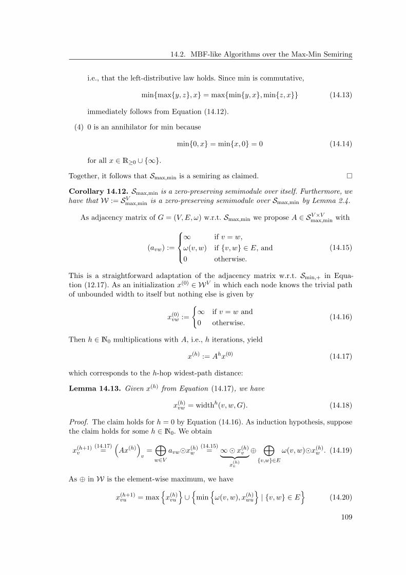
14.2. MBF-like Algorithms over the Max-Min Semiring
i.e., that the left-distributive law holds. Since min is commutative,
minmaxy, z, x = maxminy, x,minz, x (14.13)
immediately follows from Equation (14.12).
(4) 0 is an annihilator for min because
min0, x = minx, 0 = 0 (14.14)
for all x ∈ R≥0 ∪ ∞.
Together, it follows that Smax,min is a semiring as claimed.
Corollary 14.12. Smax,min is a zero-preserving semimodule over itself. Furthermore, wehave that W := SVmax,min is a zero-preserving semimodule over Smax,min by Lemma 2.4.
As adjacency matrix of G = (V,E, ω) w.r.t. Smax,min we propose A ∈ SV×Vmax,min with
(avw) :=
∞ if v = w,
ω(v, w) if v, w ∈ E, and
0 otherwise.
(14.15)
This is a straightforward adaptation of the adjacency matrix w.r.t. Smin,+ in Equa-tion (12.17). As an initialization x(0) ∈ WV in which each node knows the trivial pathof unbounded width to itself but nothing else is given by
x(0)vw :=
∞ if v = w and
0 otherwise.(14.16)
Then h ∈ N0 multiplications with A, i.e., h iterations, yield
x(h) := Ahx(0) (14.17)
which corresponds to the h-hop widest-path distance:
Lemma 14.13. Given x(h) from Equation (14.17), we have
x(h)vw = widthh(v, w,G). (14.18)
Proof. The claim holds for h = 0 by Equation (14.16). As induction hypothesis, supposethe claim holds for some h ∈ N0. We obtain
x(h+1)v
(14.17)=
(Ax(h)
)v
=⊕w∈V
avwx(h)w
(14.15)= ∞ x(h)
v︸ ︷︷ ︸x(h)v
⊕⊕
v,w∈E
ω(v, w)x(h)w . (14.19)
As ⊕ in W is the element-wise maximum, we have
x(h+1)vu = max
x(h)vu
∪
minω(v, w), x(h)
wu
| v, w ∈ E
(14.20)
109

Chapter 14. A Collection of MBF-like Algorithms
and the induction hypothesis yields
x(h+1)vu = max
widthh(v, u,G)
∪
minω(v, w),widthh(w, u,G)
| v, w ∈ E
,
(14.21)
which is exactly widthh+1(v, u,G).
Example 14.14 (Single-Source Widest Paths). Single-Source Widest Paths (SSWP)asks for, given a weighted graph G = (V,E, ω), a designated source node s ∈ V , andh ∈ N0, the h-hop widest-path distance widthh(s, v,G) for every v ∈ V . It is solved by
an MBF-like algorithm with S =M = Smax,min, r = id, and x(0)s =∞ and x
(0)v = 0 for
all v 6= s.
Example 14.15 (All-Pairs Widest Paths). All-Pairs Widest Paths (APWP) asks for,given G = (V,E, ω) and h ∈ N0, widthh(v, w,G) for all v, w ∈ V . APWP is MBF-like;it is solved by choosing S = Smax,min, M = W, r = id, and x(0) from Equation (14.16)by Lemma 14.13.
Example 14.16 (Multi-Source Widest Paths). The Multi-Source Widest Paths (MSWP)problem is to determine, for each node, the h-hop widest path distance to all nodes in adesignated set S ⊆ V of source nodes. This is solved by the same MBF-like algorithm as
for APWP in Example 14.15 when changing x(0) to x(0)vw =∞ if v = w ∈ S and x
(0)vw = 0
otherwise.
14.3 MBF-like Algorithms over the All-Paths Semiring
Mohri discusses the k-SDP, where each v ∈ V is required to find the k shortest paths toa designated source node s ∈ V , in the light of his algebraic framework for distance com-putations [115]. Our framework captures this application as well, but requires a differentsemiring than Smin,+: While Smin,+ suffices for many applications, see Section 14.1, itcannot distinguish between different paths of the same length. This is a problem in thek-SDP, because there may be multiple paths of the same length among the k shortest.
Observation 14.17. No semimodule M over Smin,+ can overcome this issue: Theleft-distributive law for semimodules, see Equation (2.9), requires, for all x ∈ M ands, s′ ∈ Smin,+, that sx ⊕ s′x = (s ⊕ s′)x. Consider different paths π 6= π′ ending in thesame node with ω(π) = s = s′ = ω(π′). W.r.t. Smin,+ and M, the left-distributive lawyields sx ⊕ s′x = mins, s′ x, i.e., propagating x over π, over π′, or over both andthen aggregating must be indistinguishable in the case of s = s′.
This does not mean that the framework of MBF-like algorithms cannot be applied;it merely indicates that we need a more powerful semiring than Smin,+. The motivationof this section is to generalize Smin,+ to the all-paths semiring Pmin,+ and add it tothe toolbox. With Pmin,+ in place, the established machinery becomes available: pick asemimodule (in our examples, Pmin,+ itself suffices) and define a representative projection.We demonstrate this for the k-SDP and a variant.
110
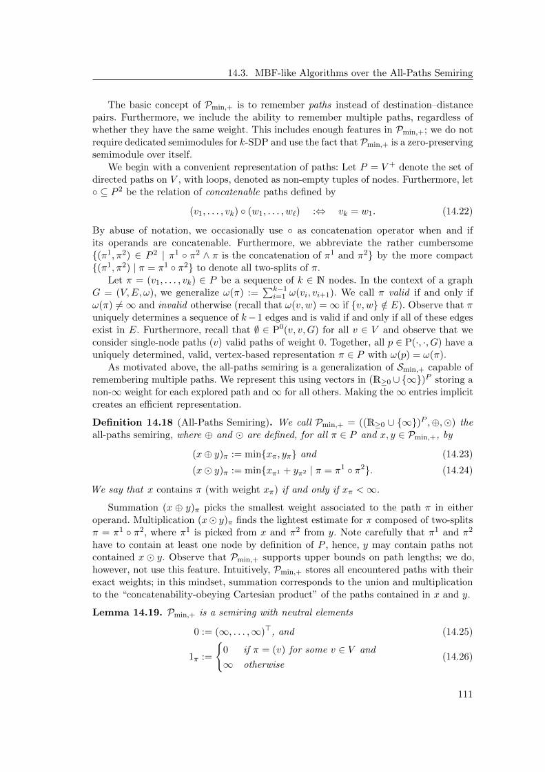
14.3. MBF-like Algorithms over the All-Paths Semiring
The basic concept of Pmin,+ is to remember paths instead of destination–distancepairs. Furthermore, we include the ability to remember multiple paths, regardless ofwhether they have the same weight. This includes enough features in Pmin,+; we do notrequire dedicated semimodules for k-SDP and use the fact that Pmin,+ is a zero-preservingsemimodule over itself.
We begin with a convenient representation of paths: Let P = V + denote the set ofdirected paths on V , with loops, denoted as non-empty tuples of nodes. Furthermore, let ⊆ P 2 be the relation of concatenable paths defined by
(v1, . . . , vk) (w1, . . . , w`) :⇔ vk = w1. (14.22)
By abuse of notation, we occasionally use as concatenation operator when and ifits operands are concatenable. Furthermore, we abbreviate the rather cumbersome(π1, π2) ∈ P 2 | π1 π2 ∧ π is the concatenation of π1 and π2 by the more compact(π1, π2) | π = π1 π2 to denote all two-splits of π.
Let π = (v1, . . . , vk) ∈ P be a sequence of k ∈ N nodes. In the context of a graphG = (V,E, ω), we generalize ω(π) :=
∑k−1i=1 ω(vi, vi+1). We call π valid if and only if
ω(π) 6=∞ and invalid otherwise (recall that ω(v, w) =∞ if v, w /∈ E). Observe that πuniquely determines a sequence of k−1 edges and is valid if and only if all of these edgesexist in E. Furthermore, recall that ∅ ∈ P0(v, v,G) for all v ∈ V and observe that weconsider single-node paths (v) valid paths of weight 0. Together, all p ∈ P(·, ·, G) have auniquely determined, valid, vertex-based representation π ∈ P with ω(p) = ω(π).
As motivated above, the all-paths semiring is a generalization of Smin,+ capable ofremembering multiple paths. We represent this using vectors in (R≥0 ∪ ∞)P storing anon-∞ weight for each explored path and∞ for all others. Making the∞ entries implicitcreates an efficient representation.
Definition 14.18 (All-Paths Semiring). We call Pmin,+ = ((R≥0 ∪ ∞)P ,⊕,) theall-paths semiring, where ⊕ and are defined, for all π ∈ P and x, y ∈ Pmin,+, by
(x⊕ y)π := minxπ, yπ and (14.23)
(x y)π := minxπ1 + yπ2 | π = π1 π2. (14.24)
We say that x contains π (with weight xπ) if and only if xπ <∞.
Summation (x ⊕ y)π picks the smallest weight associated to the path π in eitheroperand. Multiplication (x y)π finds the lightest estimate for π composed of two-splitsπ = π1 π2, where π1 is picked from x and π2 from y. Note carefully that π1 and π2
have to contain at least one node by definition of P , hence, y may contain paths notcontained x y. Observe that Pmin,+ supports upper bounds on path lengths; we do,however, not use this feature. Intuitively, Pmin,+ stores all encountered paths with theirexact weights; in this mindset, summation corresponds to the union and multiplicationto the “concatenability-obeying Cartesian product” of the paths contained in x and y.
Lemma 14.19. Pmin,+ is a semiring with neutral elements
0 := (∞, . . . ,∞)>, and (14.25)
1π :=
0 if π = (v) for some v ∈ V and
∞ otherwise(14.26)
111
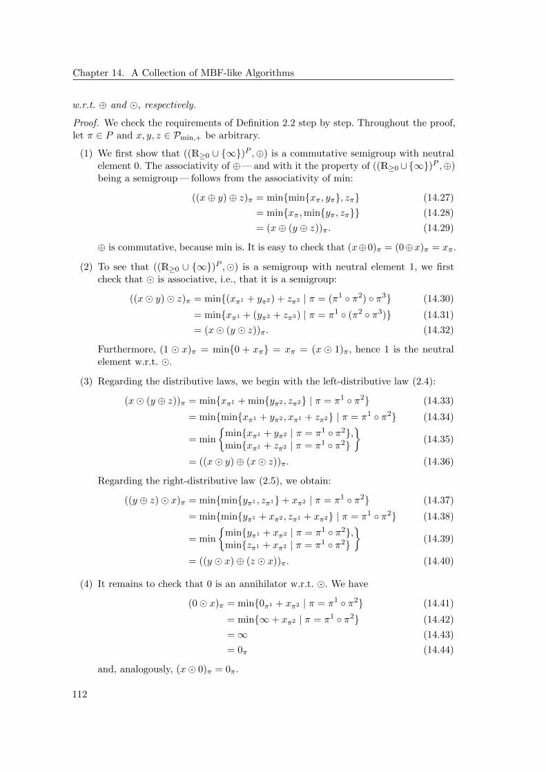
Chapter 14. A Collection of MBF-like Algorithms
w.r.t. ⊕ and , respectively.
Proof. We check the requirements of Definition 2.2 step by step. Throughout the proof,let π ∈ P and x, y, z ∈ Pmin,+ be arbitrary.
(1) We first show that ((R≥0 ∪ ∞)P ,⊕) is a commutative semigroup with neutralelement 0. The associativity of ⊕— and with it the property of ((R≥0 ∪∞)P ,⊕)being a semigroup — follows from the associativity of min:
((x⊕ y)⊕ z)π = minminxπ, yπ, zπ (14.27)
= minxπ,minyπ, zπ (14.28)
= (x⊕ (y ⊕ z))π. (14.29)
⊕ is commutative, because min is. It is easy to check that (x⊕0)π = (0⊕x)π = xπ.
(2) To see that ((R≥0 ∪ ∞)P ,) is a semigroup with neutral element 1, we firstcheck that is associative, i.e., that it is a semigroup:
((x y) z)π = min(xπ1 + yπ2) + zπ3 | π = (π1 π2) π3 (14.30)
= minxπ1 + (yπ2 + zπ3) | π = π1 (π2 π3) (14.31)
= (x (y z))π. (14.32)
Furthermore, (1 x)π = min0 + xπ = xπ = (x 1)π, hence 1 is the neutralelement w.r.t. .
(3) Regarding the distributive laws, we begin with the left-distributive law (2.4):
(x (y ⊕ z))π = minxπ1 + minyπ2 , zπ2 | π = π1 π2 (14.33)
= minminxπ1 + yπ2 , xπ1 + zπ2 | π = π1 π2 (14.34)
= min
minxπ1 + yπ2 | π = π1 π2,minxπ1 + zπ2 | π = π1 π2
(14.35)
= ((x y)⊕ (x z))π. (14.36)
Regarding the right-distributive law (2.5), we obtain:
((y ⊕ z) x)π = minminyπ1 , zπ1+ xπ2 | π = π1 π2 (14.37)
= minminyπ1 + xπ2 , zπ1 + xπ2 | π = π1 π2 (14.38)
= min
minyπ1 + xπ2 | π = π1 π2,minzπ1 + xπ2 | π = π1 π2
(14.39)
= ((y x)⊕ (z x))π. (14.40)
(4) It remains to check that 0 is an annihilator w.r.t. . We have
(0 x)π = min0π1 + xπ2 | π = π1 π2 (14.41)
= min∞+ xπ2 | π = π1 π2 (14.42)
=∞ (14.43)
= 0π (14.44)
and, analogously, (x 0)π = 0π.
112

14.3. MBF-like Algorithms over the All-Paths Semiring
Together, Pmin,+ is a semiring as claimed.
Corollary 14.20. Pmin,+ is a zero-preserving semimodule over itself.
Computations in a graph G = (V,E, ω) w.r.t. Pmin,+ require an adjacency matrixA ∈ PV×Vmin,+. We propose the following generalization of Equation (12.17) with
(avw)π :=
1π if v = w,
ω(v, w) if π = (v, w), and
∞ otherwise.
(14.45)
On the diagonal, avv = 1 contains exactly the zero-hop paths of weight 0; all non-trivialpaths are “unknown” in avv, i.e., accounted for with an infinite weight. An entry avwwith v 6= w contains, if present, only the edge v, w, represented by the path (v, w) ofweight ω(v, w); no other path is contained in avw. An initialization where each node vknows only the zero-hop path (v) is represented by the vector x(0) ∈ PVmin,+ with
(x(0)v
)π
:=
0 if π = (v) and
∞ otherwise.(14.46)
Then h ∈ N0 multiplications of x(0) with A, i.e., h iterations, yield
x(h) := Ahx(0) (14.47)
and x(h)v contains exactly the h-hop paths beginning in v with their according weights:
Lemma 14.21. Let x(h) be defined as in Equation (14.46), w.r.t. the graph G = (V,E, ω).Then for all v ∈ V and π ∈ P(
x(h)v
)π
=
ω(π) if π ∈ Ph(v, ·, G) and
∞ otherwise.(14.48)
Proof. We prove the claim by induction. The claim holds for h = 0 by Equation (14.46).As induction hypothesis, suppose the claim holds for h ∈ N0. The induction step yields
x(h+1)v
(14.47)=
(Ax(h)
)v
=⊕w∈V
avwx(h)w
(14.45)= avv︸︷︷︸
1
x(h)v ⊕
⊕v,w∈E
avwx(h)w . (14.49)
We have avvx(h)v = 1x
(h)v = x
(h)v by construction, i.e., avvx
(h)v contains exactly the properly
weighted h-hop paths beginning at v by the induction hypothesis. Next, consider v, w ∈E. By induction, x
(h)w contains exactly the h-hop paths beginning in w and avw contains
only the edge v, w of weight ω(v, w) by Equation (14.45). Hence, avwx(h) contains all
(h+ 1)-hop paths beginning with v, w. Due to Equation (14.49) and to
Ph+1(v, ·, G) = Ph(v, ·, G) ∪⋃
v,w∈E
(v, w) π | π ∈ Ph(w, ·, G)
, (14.50)
x(h+1)v contains exactly the properly weighted (h+ 1)-hop paths, as claimed.
113

Chapter 14. A Collection of MBF-like Algorithms
With the all-paths semiring Pmin,+ established, we turn to the k-SDP, our motivationfor adding Pmin,+ to the toolbox of MBF-like algorithms in the first place.
Definition 14.22 (k-Shortest Distance Problem [115]). Given a graph G = (V,W, ω)and a designated source vertex s ∈ V , the k-Shortest Distance Problem (k-SDP) asks:For each node v ∈ V and considering all v-s-paths, what are the weights of the k lightestsuch paths? In the k-Distinct-Shortest Distance Problem (k-DSDP), the path weightshave to be distinct.
With S = M = Pmin,+ and r = id, we already have an inefficient solution for thek-SDP and the k-DSDP in place: This corresponds to collecting all h-hop paths and thenpicking only k at each node. In terms of efficiency, however, this is like solving SSSP byfirst solving APSP and then discarding almost all distances. In order to solve the k-SDPmore efficiently, we require a representative projection that reduces the abundance ofpaths stored in an unfiltered x(h) to the relevant ones.
Observe that with the above definitions of A and x(h), we always associate a path πwith either its weight ω(π) or with ∞; in particular, invalid paths always are associatedwith ∞. Formally, G induces a subsemiring of Pmin,+. Besides being an interesting ob-servation, these properties are required for the representative projections defined below —r breaks for the k-DSDP when facing inconsistent non-∞ values for the same path — sowe formalize them. Let G = (V,E, ω) a graph and let D(G) ⊂ (R≥0 ∪ ∞)P be therestriction of (R≥0 ∪ ∞)P to exact path weights and ∞:
xπ ∈ ω(π),∞; (14.51)
recall that ω(π) =∞ for all paths π invalid w.r.t. G.
Definition 14.23 (Graph-Induced All-Paths Semiring). Let G be a graph and D(G) ⊂(R≥0 ∪ ∞)P as above. Then we refer to Pmin,+(G) := (D(G),⊕,) as the all-pathssemiring induced by G, where ⊕ and are the same as in Definition 14.18.
The next step is to show that Pmin,+(G) is a semiring. It actually is a subsemiring ofPmin,+. We do, however, not use that property and hence refrain from formally introducingthe according definitions.
Lemma 14.24. Pmin,+(G) is a semiring.
Proof. Fix a graph G = (V,E, ω). We show that D(G) is closed under ⊕ and . Considerx, y ∈ D(G) and let π ∈ P be a path. Hence, we have xπ, yπ ∈ ω(π),∞ if π is validand xπ = yπ =∞ if π is invalid in G; recall that we defined ω(π) =∞ for invalid paths.
(1) Consider x ⊕ y. It directly follows from xπ, yπ ∈ ω(π),∞ that (x ⊕ y)π =minxπ, yπ ∈ ω(π),∞. Hence, (x⊕ y) ∈ D(G).
(2) Regarding multiplication, we have (x y)π = xπ1 + yπ2 for some two-split of π.Due to xπ1 ∈ ω(π1),∞ and yπ2 ∈ ω(π2),∞, we obtain (x y)π = xπ1 + yπ2 ∈ω(π1) +ω(π2),∞ = ω(π),∞. If π is invalid in G, π1 or π2 must be invalid and(x y)π = xπ1 + yπ2 =∞ follows.
Also observe that 0, 1 ∈ D(G) for 0 and 1 from Lemma 14.19. Together, it follows fromLemma 14.19 that Pmin,+(G) is a semiring.
114

14.3. MBF-like Algorithms over the All-Paths Semiring
Corollary 14.25. Pmin,+(G) is a zero-preserving semimodule over itself.
Observe that we have A ∈ PV×Vmin,+(G) as well as x(0) ∈ PVmin,+(G). It follows thatLemma 14.21 holds for Pmin,+(G) as much as it does for Pmin,+. Furthermore, observethat the restriction to Pmin,+(G) happens implicitly, simply by starting with the aboveinitialization. There is no information about Pmin,+(G) that needs to be distributed inthe graph in order to run an MBF-like algorithm over Pmin,+(G).
With Pmin,+(G) in place, we turn our attention back to the k-SDP. Specifically, weneed a representative projection that, given the abundance of possible paths collectedby the all-paths semimodule, discards all but the relevant paths. Relevant in this casemeans to keep the k shortest v-s-paths. In order to formalize this, let P (v, w, x) denote,for x ∈ Pmin,+(G) and v, w ∈ V , the set of v-w-paths contained in x:
P (v, w, x) := π ∈ P | π is a v-w-path with xπ 6=∞. (14.52)
Order P (v, w, x) ascendingly w.r.t. the weights xπ, breaking ties using lexicographicalorder on P . Then let Pk(v, w, x) denote the set of the first at most k entries of thatsequence:
Pk(v, w, x) := π | (xπ, π) is among k smallest of (xπ′ , π′) | π′ ∈ P (v, w, x). (14.53)
We define the (representative, see below) projection r : Pmin,+(G)→ Pmin,+(G) by
r(x)π :=
xπ if π ∈ Pk(v, s, x) for some v ∈ V and
∞ otherwise.(14.54)
If xπ = r(x)π we say that r keeps π and otherwise that r discards π. The projection rkeeps, for each v ∈ V , exactly the k shortest v-s-paths contained in x. Let π be a v-w-path and y ∈ Pmin,+(G) such that y contains only π, i.e., with yπ = ω(π) and yπ′ =∞for all π′ 6= π. We say that π is dominated in x if and only if r(x⊕ y)π =∞, meaningthat making π available in x does not change the outcome of filtering. Regarding thek-SDP, this is the case where either (1) π does not end in s, or (2) x contains k otherv-s-paths that are shorter than π or have the same weight as π but are lexicographicallyordered before π. While the notion of domination may seem overly complicated for thematter at hand, it sufficiently generalizes the proof for Lemma 14.27 to cover the k-SDPas well as the k-DSDP from Examples 14.28 and 14.29, respectively.
Observation 14.26. Note that r discards all paths not ending in s. Furthermore, forall paths π, we have
r(x)π = xπ or r(x)π =∞, (14.55)
i.e., r(x) ∈ Pmin,+(G) for all x ∈ Pmin,+(G), as r either keeps a path with its originalweight or discards it by setting the according entry to ∞. We also obtain that, for allv ∈ V ,
Pk(v, s, x) = Pk(v, s, r(x)) (14.56)
because Pk(v, s, x) is invariant under discarding dominated paths from x.
Following the standard approach — Lemma 13.8 — we define vectors x, y ∈ Pmin,+(G)to be equivalent if and only if their entries for Pk(·, s, x) do not differ:
∀x, y ∈ Pmin,+(G) : x ∼ y :⇔ r(x) = r(y). (14.57)
115

Chapter 14. A Collection of MBF-like Algorithms
Lemma 14.27. ∼ is a congruence relation on Pmin,+(G) with representative projection r.
Proof. Clearly, r is a projection. Below, we show in one step each that it fulfills Condi-tions (13.12) and (13.13) of Lemma 13.8. Throughout the proof, fix a graphG = (V,E, ω),let x, x′, y, y′ ∈ Pmin,+(G) be such that x ∼ x′ and y ∼ y′.
(1) We show below that r(yx) = r(yr(x)). Equation (13.12) then follows using thatr(yx) = r(yr(x)) = r(yr(x′)) = r(yx′). To see that r(yx) = r(yr(x)), we arguethat for all v-s-paths π, we either have (yx)π = (yr(x))π, or both π /∈ Pk(v, s, yx)and π /∈ Pk(v, s, yr(x)). In other words, the entries regarding π are either equal inyx and yr(x), or r discards π from yx as well as from yr(x).
Consider a v-s-path π with (yx)π 6= (yr(x))π. Observe that this implies ω(π) =(yx)π < (yr(x))π =∞ because the non-∞ entries of r(x) are a subset of those of x.Hence, π is contained in yx. By definition of , it holds that (yx)π = yπ1 + xπ2
for some partition π = π1 π2, where π1 and π2 are, for some node w, v-w- andw-s-paths, respectively. It follows from Equation (14.55) and x ∈ Pmin,+(G) that
ω(π2) = xπ2 < r(x)π2 =∞. (14.58)
Hence, π2 /∈ Pk(w, s, x), i.e., π2 is dominated in x. As Pk(w, s, r(x)) = Pk(w, s, x)by Equation (14.56), the following k v-s-paths are contained in yr(x) and in yxeach:
π1 π2 | π2 ∈ Pk(w, s, r(x)). (14.59)
We conclude that π is dominated in — and thus discarded from — both yx and yr(x),as claimed.
(2) Consider a node v ∈ V and a v-s-path π. As (x ⊕ y)π = minxπ, yπ, we haveP (v, s, x⊕ y) = P (v, s, x) ∪ P (v, s, y). In particular, it holds that Pk(v, s, x⊕ y) ⊆Pk(v, s, x) ∪ Pk(v, s, y), because if π ∈ P (v, s, x⊕ y) is dominated in x and in y, itis dominated in x⊕ y as well. Using Equation (14.56), we obtain that
Pk(v, s, x⊕ y) ⊆ Pk(v, s, x) ∪ Pk(v, s, y) = Pk(v, s, r(x)) ∪ Pk(v, s, r(y)). (14.60)
As r discards all paths not ending in s, and xπ = r(x)π for all π ∈ Pk(v, s, r(x))and, analogously, yπ = r(y)π for all π ∈ Pk(v, s, r(y)), we conclude that r(x⊕ y) =r(r(x)⊕ r(y)). Hence, r(x⊕ y) = r(r(x)⊕ r(y)) = r(r(x′)⊕ r(y′)) = r(x′⊕ y′), i.e.,r fulfills Equation (13.13).
Since x ∼ x′ and y ∼ y′ are arbitrary, r fulfills the preconditions of Lemma 13.8 and theclaim follows.
Observe that r is defined such that it maintains the k shortest v-s-paths for all v ∈ V ,
potentially storing k|V | paths instead of just k. Intuitively, one could argue that rV x(h)v
only needs to contain k paths since they all start in v, which is what the algorithm shouldactually be doing. This objection is correct in that this is what actually happens when
running the algorithm with initialization x(0): By Lemma 14.21, x(h)v contains the h-hop
shortest paths starting in v and r removes all that do not end in s or are too long. Onthe other hand, the objection is misleading. In order for r to behave correctly w.r.t. all
116

14.4. MBF-like Algorithms over the Boolean Semiring
x ∈ Pmin,+(G) — including those less nicely structured than x(h)v where all paths start
at v— we must define r as it is, otherwise the proof of Lemma 14.27 fails for mixedstarting-node inputs.
Example 14.28 (k-Shortest Distance Problem). The k-SDP, compare Definition 14.22,is solved by an MBF-like algorithm A with S = M = Pmin,+(G), the representativeprojection and congruence relation defined in Equations (14.54) and (14.57), the choicesof A and x(0) from Equations (14.45) and (14.46), and h = SPD(G) iterations.
By Lemma 14.21 and due to h = SPD(G), x(h)v contains all v-s-paths with their
correct weights. Hence, Ah(G)v = (rV x(h))v contains the subset of those paths thek-SDP asks for. We remark that solving a generalization of the k-SDP looking for thek shortest h-hop distances is straightforward using h iterations. Furthermore, note thatour approach reveals the actual paths along with their weights.
Example 14.29 (k-Distinct-Shortest Distance Problem). The k-DSDP from Defini-tion 14.22 is solved by an MBF-like algorithm analogous to that for the k-SDP fromExample 14.28.
In order for this to work, the definition of Pk(v, w, x) in Equation (14.53) needs to beadjusted. For each of the k smallest weights in x, the modified Pk(v, w, x) contains onlyone representative: the path contained in x of that weight that is first w.r.t. lexicographicalorder on P . This results in
P ′k(v, w, x) := π | xπ is among the k smallest of xπ′ | π′ ∈ P (v, w, x) and (14.61)
Pk(v, w, x) := π | π is lexicographically first of π′ ∈ P ′k(v, w, x) | xπ′ = xπ. (14.62)
Observe that this changes the meaning of π being dominated in x. With that in mind, Ob-servation 14.26 and the proof of Lemma 14.27 work without modification when replacingEquation (14.53) with Equations (14.61)–(14.62).
14.4 MBF-like Algorithms over the Boolean Semiring
A well-known semiring is the Boolean semiring B := (B,∨,∧) and by Lemma 2.4, BV isa zero-preserving semimodule over B. It can be used to check for connectivity in a graph1
using the adjacency matrix
(avw) :=
1 if v = w,
1 if v, w ∈ E, and
0 otherwise
(14.63)
together with initial values
x(0)vw :=
1 if v = w and
0 otherwise(14.64)
indicating that each node v ∈ V is connected to itself. Induction over h reveals that(Ahx(0)
)vw
= 1 ⇔ Ph(v, w,G) 6= ∅. (14.65)
1In this section, we drop the assumption that graphs are connected.
117

Chapter 14. A Collection of MBF-like Algorithms
Example 14.30 (Connectivity). Given a graph, we want to check which pairs of nodesare connected by paths of at most h hops. This is solved by an MBF-like algorithm usingS = B, M = BV , r = id, and x(0) from Equation (14.64).
Example 14.30 directly generalizes to single-source and multi-source connectivityvariants using a filter function that discards non-sources.
118

CHAPTER 15
An Oracle for MBF-like Queries
Our goal is to solve distance problems in a graph G using polylog n depth and as littlework as possible. In order to keep the number of iterations low, we augment G withCohen’s (d, ε)-hop set [34]: a small number of additional (weighted) edges for G, such thatfor all v, w ∈ V , distd(v, w,G) ≤ (1 + ε) dist(v, w,G), where d, ε−1 ∈ polylog n. Cohen’salgorithm is sufficiently efficient in terms of depth, work, and number of additionaledges. Our presentation, however, is independent from the hop-set algorithm: We onlyrequire that distd(·, ·, G) is a (1 + ε)-approximation of dist(·, ·, G), i.e., that d iterationsof MBF-like algorithms obtain good distance approximations, which is a cornerstonefor algorithms of polylog n depth. As detailed in Observation 12.1, however, distd(·, ·, G)does not obey the triangle inequality and SPD(G) remains unaffected by additionalhop-set edges. Unfortunately, the triangle inequality is vital to the problems that wediscuss: approximate metrics and FRT embeddings in Chapters 16 and 17, respectively.
Hence, we reduce the SPD, accepting a slight increase in stretch. After augmentingG with the hop set, we embed it into a complete graph H on the same node set such thatSPD(H) ∈ O(log2 n) and dist(v, w,G) ≤ dist(v, w,H) ∈ (1 + o(1)) dist(v, w,G). Wherehop sets preserve distances exactly and ensure the existence of approximately shortestpaths with few hops, H preserves distances approximately but guarantees that we obtainexact shortest paths with few hops. This is discussed in Section 15.1.
This approach keeps algorithms of polylog n depth in reach, resolves the issue withthe triangle inequality, and still guarantees (1 + o(1))-approximate distances w.r.t. G.Unfortunately, however, H is a complete graph, so directly working on it or even storingit in memory imposes Ω(n2) work. Hence, we improve our approach to allow low-workalgorithms while still maintaining the requirement of polylog n depth. In particular, wewant to sample an FRT embedding using near-linear work in m, see Chapter 17. Oursolution is an oracle for MBF-like queries over Smin,+; we develop it in Sections 15.2–15.3.Given an MBF-like algorithm A over Smin,+, a graph G, and a number of iterations h,the oracle answers with Ah(H). Put differently, the oracle can simulate A in H withoutexplicitly constructing H, instead, it internally works on G. The oracle heavily exploitsthe properties of MBF-like algorithms from Chapter 13 and simulates each iteration of Ain H using polylogarithmically many iterations of A in G. As h = SPD(H) ∈ O(log2 n)iterations suffice, Ah(H) can be determined with only a polylogarithmic overhead w.r.t.a single iteration in G. This keeps a work of O(m) in reach while maintaining polylog ndepth, obeying the triangle inequality, and (1 + o(1))-approximating distances.
15.1 The Simulated Graph H
After augmenting G with the hop set, we embed it into a complete graph H on the samenode set so that SPD(H) ∈ O(log2 n), keeping the stretch limited. Since our construction

Chapter 15. An Oracle for MBF-like Queries
requires to first add a hop set to G, assume for the sake of presentation that G alreadycontains a (d, ε)-hop set for fixed ε ∈ R>0 and d ∈ N throughout this chapter.
We begin the construction of H by sampling levels for the vertices V : Every vertexstarts at level 0. In step λ ≥ 1, each vertex in level λ − 1 is raised to level λ withprobability 1
2 . We continue until the first step Λ+1 where no node is sampled. λ(v) refersto the level of v ∈ V and we define the level of an edge e ∈ E as λ(e) := minλ(v) | v ∈ e,the minimal level of its incident vertices. In the following, we abbreviate λ(v, w) :=λ(v, w).Lemma 15.1. W.h.p., Λ ∈ O(log n).
Proof. For a constant c ∈ R≥1, v ∈ V has λ(v) < c log n ∈ O(log n) with a probabilityof at least 1 − (1
2)c logn = 1 − n−c, i.e., w.h.p. By Lemma 2.7, this w.h.p. holds for allnodes and the claim follows.
The idea is to use the levels in the following way. We devise a complete graph Hon V . An edge of H of level λ is weighted with the d-hop distance between its endpointsin G— a (1+ ε)-approximation of their exact distance because G contains a (d, ε)-hop setby assumption — multiplied with a penalty of (1 + ε)Λ−λ. This way, high-level edges are“more attractive” for shortest paths, because they receive exponentially smaller penalties.
Definition 15.2 (Simulated graph H). Let G = (V,E, ω) be a graph that contains a(d, ε)-hop set with levels sampled as above. We define the complete graph H as
H :=
(V,
(V
2
), ωΛ
)(15.1)
ωΛ(v, w) := (1 + ε)Λ−λ(v,w) distd(v, w,G). (15.2)
We formalize the notion of high-level edges being “more attractive” than low-levelpaths. In H, any min-hop shortest v-w-path is exclusively comprised of edges of levelλ(v, w) or higher; no min-hop shortest path’s level locally decreases. Therefore, all min-hop shortest paths can be split into two subpaths, the first of nondecreasing and thesecond of nonincreasing level.
Lemma 15.3. Consider v, w ∈ V , λ = λ(v, w), and p ∈ MHSP(v, w,H). Then all edgesof p have level at least λ.
Proof. The case λ = 0 is trivial. Consider 1 ≤ λ ≤ Λ and, for the sake of contradiction,let q be a non-trivial maximal subpath of p containing only edges of level strictly lessthan λ. Observe that q ∈ MHSP(v′, w′, H) for some v′, w′ ∈ V with λ(v′), λ(w′) ≥ λ. Wehave
ωΛ(q) ≥ (1 + ε)Λ−(λ−1) dist(v′, w′, G) (15.3)
because q only uses edges of level at most λ−1, which all receive a multiplicative penaltyof at least (1 + ε)Λ−(λ−1) in ωΛ. However, the edge e = v′, w′ has level λ(v′, w′) ≥ λand weight
ωΛ(e) ≤ (1 + ε)Λ−λ distd(v′, w′, G) ≤ (1 + ε)Λ−(λ−1) dist(v′, w′, G) ≤ ωΛ(q) (15.4)
because G contains a (d, ε)-hop set. As q is a min-hop shortest path, we have q = e,contradicting the assumption that q only contains edges of level λ− 1 or less.
120

15.1. The Simulated Graph H
Having established that edge levels in min-hop shortest paths are first nondecreasingand then nonincreasing, the next step is to limit the number of hops spent on each level.
Lemma 15.4. Consider vertices v and w of H with λ(v), λ(w) ≥ λ. Then w.h.p., oneof the following statements holds:
hop(v, w,H) ∈ O(log n) or (15.5)
∀p ∈ MHSP(v, w,H) ∃e ∈ p : λ(e) ≥ λ+ 1. (15.6)
Proof. Condition on the event EVλ that Vλ ⊆ V , with v, w ∈ Vλ, is the set of nodes withlevel λ or higher, with level λ+ 1 not yet sampled. Let
Hλ :=
(Vλ,
(Vλ2
), ωλ
)with (15.7)
ωλ(v, w) := (1 + ε)Λ−λ distd(v, w,G) (15.8)
denote the subgraph of H spanned by Vλ and capped at level λ.
Consider p ∈ MHSP(v, w,Hλ). Observe that P[λ(u) ≥ λ+1 | EVλ ] = 12 independently
for all u ∈ Vλ, and hence P[λ(e) ≥ λ+ 1 | EVλ ] = 14 for all e ∈ p. The latter probability
holds independently for every other edge of p. If |p| ≥ 2c log4/3 n+ 1 for some choice ofc ∈ R≥1, the probability that p contains no edge of level λ+ 1 or higher is bounded fromabove by (3
4)b|p|/2c ≤ (34)(|p|−1)/2 = (3
4)c log4/3 n = n−c, so p contains such an edge w.h.p.
Fix an arbitrary p ∈ MHSP(v, w,Hλ). Let Ep denote the event that p contains anedge of level at least λ + 1 or fulfills |p| ∈ O(log n); as argued above, Ep occurs w.h.p.Note that we cannot directly apply the union bound and Lemma 2.7 to deduce a similarstatement for all q ∈ MHSP(v, w,Hλ) because |MHSP(v, w,Hλ)| is not polynomiallybounded. Instead, we argue that if Ep holds, it follows that all q ∈ MHSP(v, w,H) mustbehave as claimed.
To show that all q ∈ MHSP(v, w,H) fulfill (15.5) or (15.6) under the assumption thatEp holds for the choice of p fixed above, recall that q only uses edges of level λ or higherby Lemma 15.3. Furthermore, observe that ωΛ(q) ≤ ωΛ(p) because q is a shortest pathin H, that ωλ(p) ≤ ωλ(q) because p is a shortest path in Hλ, and that ωΛ(p) ≤ ωλ(p)for all p ∈ P(v, w,Hλ) by construction of H and Hλ. If q contains an edge of level λ+ 1or higher, (15.6) holds for q. Otherwise, q uses only edges that are exactly of level λ. Weconclude ωλ(q) = ωΛ(q) and distinguish two cases:
Case 1 If |p| ∈ O(log n), we have
ωΛ(p) ≤ ωλ(p) ≤ ωλ(q) = ωΛ(q), (15.9)
and ωΛ(q) = ωΛ(p) and |q| ≤ |p| both follow from q ∈ MHSP(v, w,H). It followsfrom the case premise that |q| ∈ O(log n), i.e., that (15.5) holds.
Case 2 If p contains an edge of level λ + 1 or higher, we obtain ωΛ(p) < ωλ(p). Thisimplies
ωΛ(p) < ωλ(p) ≤ ωλ(q) = ωΛ(q), (15.10)
which contradicts q ∈ MHSP(v, w,H).
121

Chapter 15. An Oracle for MBF-like Queries
So far, we condition on EVλ . In order to remove this restriction, fix v, w ∈ V and letEvw denote the event that (15.5) or (15.6) holds for v and w. The above case distinctionshows that P[Evw | EVλ ] ≥ 1− n−c for an arbitrary c ∈ R≥1. We conclude that
P[Evw | λ(v, w) ≥ λ] =∑Vλ⊆V
P[EVλ | λ(v, w) ≥ λ]P[Evw | EVλ ] (15.11)
=∑
v,w⊆Vλ⊆V
P[EVλ | λ(v, w) ≥ λ]P[Evw | EVλ ] (15.12)
≥∑
v,w⊆Vλ⊆V
P[EVλ | λ(v, w) ≥ λ](1− n−c) (15.13)
= (1− n−c)∑
v,w⊆Vλ⊆V
P[EVλ | λ(v, w) ≥ λ] (15.14)
= 1− n−c, (15.15)
which is the statement of the lemma.
We argue that any min-hop shortest path in H traverses every level at most twice inLemma 15.3, Lemma 15.4 states that each such traversal, w.h.p., only has a logarithmicnumber of hops, and Lemma 15.1 asserts that, w.h.p., there are only logarithmically manylevels. Together, this means that min-hop shortest paths in H have O(log2 n) hops w.h.p.Additionally, our construction limits the stretch of shortest paths in H as compared toG by (1 + ε)Λ+1, i.e., by (1 + ε)O(logn) w.h.p.
Theorem 15.5. W.h.p., SPD(H) ∈ O(log2 n) and, for all v, w ∈ V ,
dist(v, w,G) ≤ dist(v, w,H) ≤ (1 + ε)O(logn) dist(v, w,G). (15.16)
Proof. Fix a level λ. Any fixed pair of vertices of level λ or higher fulfills, w.h.p., (15.5)or (15.6) by Lemma 15.4. Since there are at most
(n2
)such pairs, w.h.p., all of them
fulfill (15.5) or (15.6) by Lemma 2.7.Let Elog denote the event that there is no higher level than Λ ∈ O(log n), which holds
w.h.p. by Lemma 15.1. Furthermore, let Eλ denote the event that all pairs of verticesof level λ or higher fulfill (15.5) or (15.6), which holds w.h.p. as argued above. ThenE := Elog ∩ E0 ∩ · · · ∩ EΛ holds w.h.p. by Lemma 2.7.
Condition on E . In particular, no min-hop shortest path whose edges all have thesame level has more than O(log n) hops. Consider some min-hop shortest path p in H.By Lemma 15.3, p has two parts: The edge level is nondecreasing in the first andnonincreasing in the second part. Hence, p can be split into at most 2Λ − 1 maximalsegments, in each of which all edges have the same level. As this holds for all min-hopshortest paths, we conclude that SPD(H) ∈ O(Λ log n) ⊆ O(log2 n), as claimed.
As for Inequality (15.16), recall that H is constructed from G = (V,E, ω), and thatG contains a (d, ε)-hop set. For all v, w ∈ V , we have
dist(v, w,H) ≤ ωΛ(v, w) ≤ (1 + ε)Λ distd(v, w,G) ≤ (1 + ε)Λ+1 dist(v, w,G) (15.17)
and dist(v, w,H) ≥ dist(v, w,G) by construction of H. Recalling that Λ ∈ O(log n) andthat we only condition on E , which occurs w.h.p., completes the proof.
122
15.2. Decomposing H
We use Cohen’s construction to obtain a (d, ε)-hop set with ε ∈ 1/ polylog n, wherethe exponent of the polylog n term is under our control [34]. A sufficiently large exponentyields
(1 + ε)O(logn)1+x≤ex⊆ eεO(logn) ⊆ e1/polylogn ⊆ 1 + 1/ polylog n, (15.18)
where the last step follows from observing that ex ≤ 1 + eux for all 0 ≤ x ≤ u. Thisupper-bounds (15.16) by
dist(v, w,G) ≤ dist(v, w,H) ∈ (1 + 1/polylog n) dist(v, w,G). (15.19)
To sum up: Given a weighted graph G, we augment G with a (d, 1/ polylog n)-hopset. After that, the d-hop distances in G readily (1 + o(1))-approximate the actualdistances in G, but these approximations may violate the triangle inequality. We fixthis by embedding into H, using geometrically sampled node levels and an exponentialpenalty on the edge weights with decreasing levels. The result is that where G preservesdistances exactly and ensures the existence of approximate shortest paths with few hops,H preserves distances (1 + o(1))-approximately but guarantees that we obtain exactshortest paths with few hops.
15.2 Decomposing H
The situation is thatH has a polylogarithmic SPD — more precisely, SPD(H) ∈ O(log2 n)w.h.p. — while at the same time (1 + o(1))-approximating the distances in G. This pavesthe way for algorithms of polylog n depth. In order to keep the work under control,however, recall that explicitly writing H into memory to directly work on it imposesΩ(n2) work which rules out subquadratic-work algorithms. In particular, this preventsus from sampling an FRT embedding using near-linear work in m, see Chapter 17.
The idea to fix this is to never explicitly write H —H is uniquely determined byG and the node levels — and to simulate iterations of an MBF-like algorithm A in H,using d iterations of A in G instead. As AG, the adjacency matrix of G, only has O(m)non-∞ entries and hd ∈ polylog n, this maintains our requirement of algorithms withpolylog n depth that still may have a work bounded by O(m). To this end, we require arepresentation of AH , the adjacency matrix of H, in terms of AG.
For the remainder of this chapter, we keep the notation of AG and AH as adjacencymatrices of G and H, and fix the semiring to be Smin,+. In order to formalize thedecomposition of AH in terms of AG motivated above, recall that by Definition 15.2 wehave
(AH)vw = ωΛ(v, w) = (1 + ε)Λ−λ(v,w) distd(v, w,G) = (1 + ε)Λ−λ(v,w)(AdG)vw. (15.20)
For a level λ ∈ 0, . . . ,Λ, denote by Pλ : MV →MV the projection to coordinates oflevel λ or higher, i.e., to Vλ := v ∈ V | λ(v) ≥ λ:
Pλ(x)v :=
xv if λ(v) ≥ λ and
⊥ otherwise.(15.21)
123
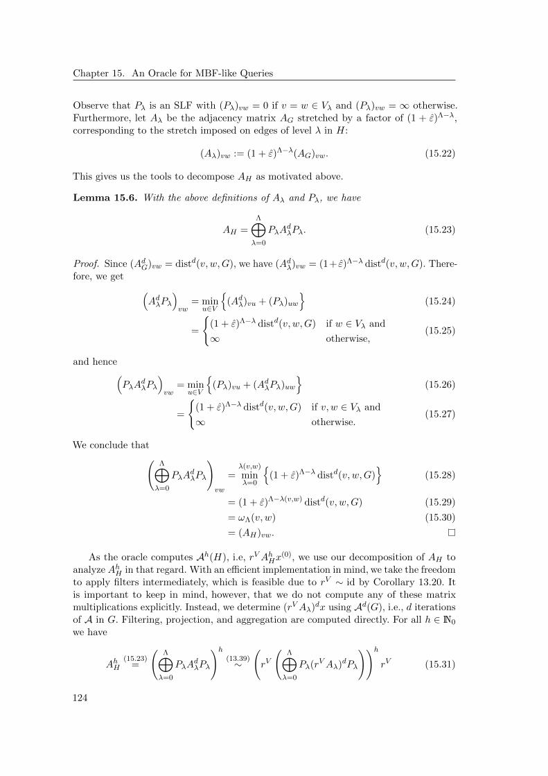
Chapter 15. An Oracle for MBF-like Queries
Observe that Pλ is an SLF with (Pλ)vw = 0 if v = w ∈ Vλ and (Pλ)vw = ∞ otherwise.Furthermore, let Aλ be the adjacency matrix AG stretched by a factor of (1 + ε)Λ−λ,corresponding to the stretch imposed on edges of level λ in H:
(Aλ)vw := (1 + ε)Λ−λ(AG)vw. (15.22)
This gives us the tools to decompose AH as motivated above.
Lemma 15.6. With the above definitions of Aλ and Pλ, we have
AH =Λ⊕λ=0
PλAdλPλ. (15.23)
Proof. Since (AdG)vw = distd(v, w,G), we have (Adλ)vw = (1+ ε)Λ−λ distd(v, w,G). There-fore, we get (
AdλPλ
)vw
= minu∈V
(Adλ)vu + (Pλ)uw
(15.24)
=
(1 + ε)Λ−λ distd(v, w,G) if w ∈ Vλ and
∞ otherwise,(15.25)
and hence(PλA
dλPλ
)vw
= minu∈V
(Pλ)vu + (AdλPλ)uw
(15.26)
=
(1 + ε)Λ−λ distd(v, w,G) if v, w ∈ Vλ and
∞ otherwise.(15.27)
We conclude that(Λ⊕λ=0
PλAdλPλ
)vw
=λ(v,w)
minλ=0
(1 + ε)Λ−λ distd(v, w,G)
(15.28)
= (1 + ε)Λ−λ(v,w) distd(v, w,G) (15.29)
= ωΛ(v, w) (15.30)
= (AH)vw.
As the oracle computes Ah(H), i.e, rVAhHx(0), we use our decomposition of AH to
analyze AhH in that regard. With an efficient implementation in mind, we take the freedomto apply filters intermediately, which is feasible due to rV ∼ id by Corollary 13.20. Itis important to keep in mind, however, that we do not compute any of these matrixmultiplications explicitly. Instead, we determine (rVAλ)dx using Ad(G), i.e., d iterationsof A in G. Filtering, projection, and aggregation are computed directly. For all h ∈ N0
we have
AhH(15.23)
=
(Λ⊕λ=0
PλAdλPλ
)h(13.39)∼
(rV
(Λ⊕λ=0
Pλ(rVAλ)dPλ
))hrV (15.31)
124

15.3. Implementation
input: A graph G = (V,E, ω) containing a (d, ε)-hop set and an MBF-like algorithm Aover Smin,+ with initialization x(0) and h ∈ N0 iterations
output: Ah(H)1: x(0) ← rV x(0)
2: for i← 1, . . . , h do . h iterations in H3: for each λ ∈ 0, . . . ,Λ in parallel do4: yλ ← Pλx
(i−1) . discard low-level nodes5: for f ← 1, . . . , d do . d iterations of A in G with stretched edge weights6: yλ ← rVAλyλ7: end for8: yλ ← Pλyλ . discard low-level nodes9: end for
10: x(i) ← rV⊕Λ
λ=0 yλ11: end for12: return x(h)
Algorithm 15.1: An Oracle for MBF-like Algorithms over Smin,+.
and hence
Ah(H)(13.18)
= rVAhHx(0) (13.11),(15.31)
=
(rV
(Λ⊕λ=0
Pλ(rVAλ)dPλ
))hrV x(0). (15.32)
Observe that we can choose h = SPD(H) ∈ O(log2 n) w.h.p. by Theorem 15.5 and recallthat w.h.p. Λ ∈ O(log n) by Lemma 15.1 and that d ∈ polylog n for an appropriatehop set [34]. Overall, we obtain hdΛ ∈ polylog n which allows us to determine A(H)with polylogarithmic depth and O(m) work, provided that the individual steps of theunderlying MBF-like algorithm can be implemented at this complexity.
15.3 Implementation
The oracle determines iterations of A in H using iterations in G while only introducinga polylogarithmic overhead w.r.t. iterations in G. With the decomposition of H fromLemma 15.6 at hand, we propose Algorithm 15.1 as an implementation of the oracle.It works as follows. Given a state vector x(i−1) ∈ MV representing the result of the(i−1)-th iteration, simulate the i-th iteration of A in H for edges of level λ, i.e., determineyλ := Pλ(rVAλ)dPλx
(i−1) by (1) discarding entries at nodes of a level smaller than λ(line 4), (2) running d iterations of A with distances stretched by (1 + ε)Λ−λ in G,applying the filter after each iteration (lines 5–7), and (3) again discarding entries atnodes with levels smaller than λ (line 8). After running this procedure in parallel forall 0 ≤ λ ≤ Λ, aggregate the results of all levels and apply the node-wise filter, i.e.,determine x(i) = rV (
⊕Λλ=0 yλ) (line 10).
Consider nodes v, w ∈ V . Since (Adλ)vw = (1 + ε)Λ−λ distd(v, w,G), the above ap-proach ensures that we propagate information between nodes v and w with the correctedge weight in the parallel run for λ = λ(v, w). Furthermore, any exchange between vand w in any run for λ > λ(v, w) is discarded by Pλ. In a run for λ < λ(v, w), however,
125

Chapter 15. An Oracle for MBF-like Queries
v and w exchange information. But observe that this information is propagated overtoo long a distance because edge weights are scaled by (1 + ε)Λ−λ > (1 + ε)Λ−λ(v,w).Hence, the “outdated” information “loses” against the copy that was propagated over theshorter distance during aggregation. Formally, it is discarded due to the left-distributivelaw of semimodules over Smin,+:(
(1 + ε)Λ−λ(v,w) x)⊕(
(1 + ε)Λ−λ x)
(15.33)
(2.9)=(
(1 + ε)Λ−λ(v,w) ⊕ (1 + ε)Λ−λ) x (15.34)
= min
(1 + ε)Λ−λ(v,w), (1 + ε)Λ−λ x (15.35)
= (1 + ε)Λ−λ(v,w) x (15.36)
for all semimodules M over Smin,+ and all x ∈M. Therefore, aggregating the results ofall levels (using ⊕) in line 10 and applying rV completes the simulation of an iterationof A in H.
The efficiency of Algorithm 15.1 crucially depends on directly implementing iterationsof A in G instead of explicitly multiplying matrices (line 6) as well as on the semimoduleM and the filter r used by A. In order to keep Theorem 15.7 general, we do not imposerestrictions onM or r. Hence, the work and depth of the basic operations — determiningrV x(0) from x(0) (line 1), rVAλy from an intermediate state y (line 6), and
⊕Λλ=0 yλ from
the individual yλ (line 10) — are parameters of the theorem. Observe that we could usesingle-purpose work and depth parameters for determining rV x(0) from x(0) instead ofreusing W and D. This, however, usually is a trivial operation and we do not wish toobstruct the presentation with further parameters.
Together, we can run any MBF-like algorithm A over Smin,+ in H with only apolylogarithmic overhead w.r.t. just a single iteration of A in G.
Theorem 15.7 (Oracle). Consider an MBF-like algorithm A using a semimodule Mover the semiring Smin,+, the representative projection r : M→M, and the initializationx(0) ∈ MV . If we can, for all 1 ≤ f ≤ d, 1 ≤ i ≤ h, and 0 ≤ λ ≤ Λ, where we mayassume Λ ∈ O(log n),
(1) compute rV x(0) from x(0) with depth D and work W (line 1),
(2) determine rVAλy from any intermediate state vector y = (rVAλ)f−1Pλx(i−1) —
corresponding to the f-th iteration w.r.t. Aλ starting at state x(i−1) — with depthD and work W (line 6), and
(3) compute rV (⊕Λ
λ=0 yλ) from the individual yλ = (PλrVAdλPλ)x(i−1), 0 ≤ λ ≤ Λ —
reflecting aggregation over all levels to complete a simulated iteration in H — usingdepth D⊕ and work W⊕ (line 10),
then we can w.h.p.
(1) determine Ah(H) using O((dW log n+W⊕)h) ⊆ O((dW+W⊕)h) work and a depthof O((dD +D⊕)h) and thus
(2) calculate A(H) using O((dW log n+W⊕) log2 n) ⊆ O(dW +W⊕) work and a depthof O((dD +D⊕) log2 n) ⊆ O(dD +D⊕).
126
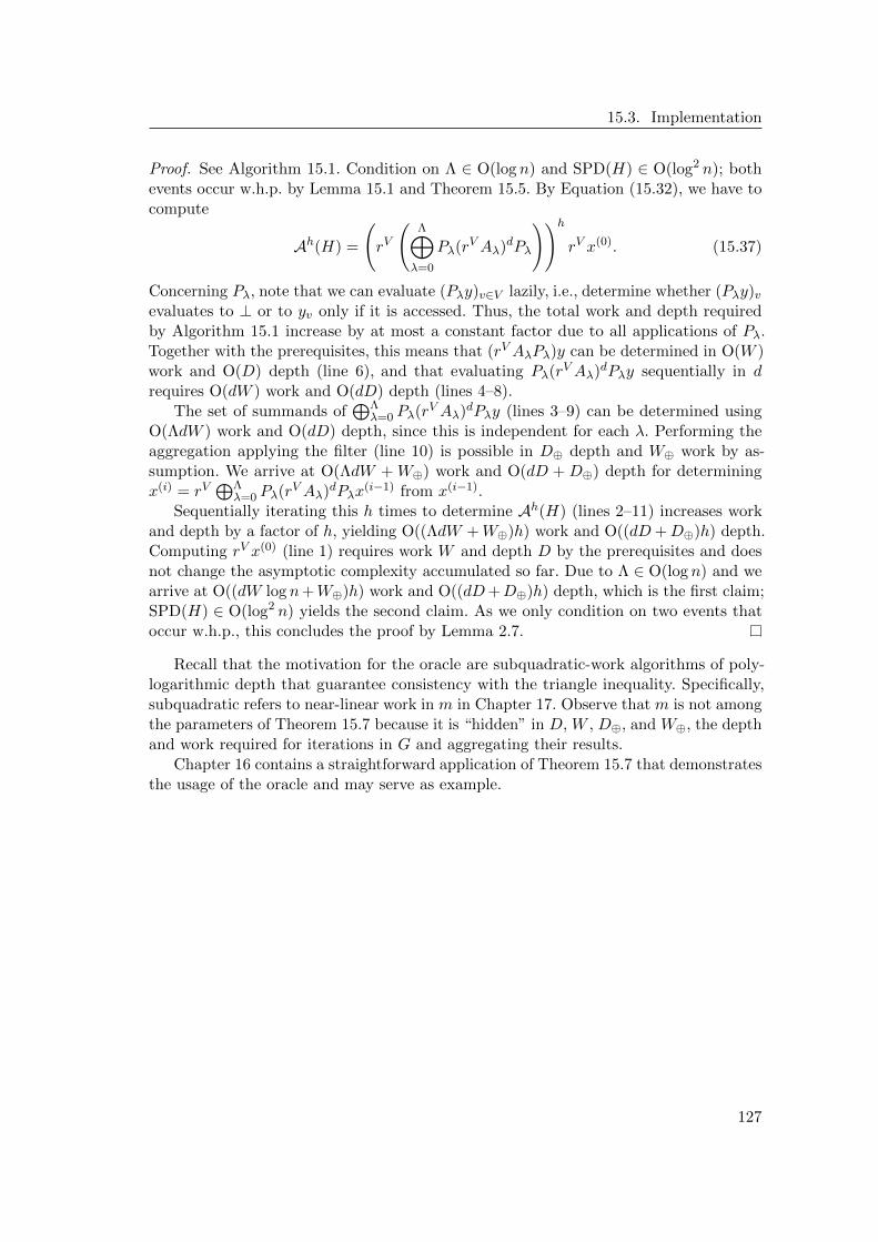
15.3. Implementation
Proof. See Algorithm 15.1. Condition on Λ ∈ O(log n) and SPD(H) ∈ O(log2 n); bothevents occur w.h.p. by Lemma 15.1 and Theorem 15.5. By Equation (15.32), we have tocompute
Ah(H) =
(rV
(Λ⊕λ=0
Pλ(rVAλ)dPλ
))hrV x(0). (15.37)
Concerning Pλ, note that we can evaluate (Pλy)v∈V lazily, i.e., determine whether (Pλy)vevaluates to ⊥ or to yv only if it is accessed. Thus, the total work and depth requiredby Algorithm 15.1 increase by at most a constant factor due to all applications of Pλ.Together with the prerequisites, this means that (rVAλPλ)y can be determined in O(W )work and O(D) depth (line 6), and that evaluating Pλ(rVAλ)dPλy sequentially in drequires O(dW ) work and O(dD) depth (lines 4–8).
The set of summands of⊕Λ
λ=0 Pλ(rVAλ)dPλy (lines 3–9) can be determined usingO(ΛdW ) work and O(dD) depth, since this is independent for each λ. Performing theaggregation applying the filter (line 10) is possible in D⊕ depth and W⊕ work by as-sumption. We arrive at O(ΛdW + W⊕) work and O(dD + D⊕) depth for determiningx(i) = rV
⊕Λλ=0 Pλ(rVAλ)dPλx
(i−1) from x(i−1).Sequentially iterating this h times to determine Ah(H) (lines 2–11) increases work
and depth by a factor of h, yielding O((ΛdW +W⊕)h) work and O((dD+D⊕)h) depth.Computing rV x(0) (line 1) requires work W and depth D by the prerequisites and doesnot change the asymptotic complexity accumulated so far. Due to Λ ∈ O(log n) and wearrive at O((dW log n+W⊕)h) work and O((dD+D⊕)h) depth, which is the first claim;SPD(H) ∈ O(log2 n) yields the second claim. As we only condition on two events thatoccur w.h.p., this concludes the proof by Lemma 2.7.
Recall that the motivation for the oracle are subquadratic-work algorithms of poly-logarithmic depth that guarantee consistency with the triangle inequality. Specifically,subquadratic refers to near-linear work in m in Chapter 17. Observe that m is not amongthe parameters of Theorem 15.7 because it is “hidden” in D, W , D⊕, and W⊕, the depthand work required for iterations in G and aggregating their results.
Chapter 16 contains a straightforward application of Theorem 15.7 that demonstratesthe usage of the oracle and may serve as example.
127

Chapter 15. An Oracle for MBF-like Queries
128

CHAPTER 16
Parallel Approximate Metrics
Our oracle for MBF-like queries from Chapter 15 permits the efficient simulation ofMBF-like algorithms in a graph H, which (1 + o(1))-approximates distances in G. Theentire simulation only has polylogarithmic overhead w.r.t. a single iteration inG, providedthat we first add an appropriate hop set to G. Querying the oracle with the MBF-likealgorithm APSP — see Example 14.6 — hence yields a (1 + o(1))-approximate metric ofdist(·, ·, G) w.r.t. Definition 12.2; note that respecting the triangle inequality is criticalfor this problem.
Determining the hop set and querying the oracle with APSP together requires poly-logarithmic depth and O(nm+n2+ε) work, compare Corollary 16.6. In sparse graphs, thisis much more work-efficient than the naive approach using O(n3 log n) work — squaringthe adjacency matrix dlog2 ne times — for obtaining dist(·, ·, G) exactly.
Instead of APSP, however, we use MSSP below. MSSP determines dist(s, v,G) for alls ∈ S and v ∈ V , where S ⊆ V is a designated set of source nodes, compare Example 14.7.This is a slight generalization of APSP — APSP is MSSP with S = V — that gives usthe flexibility to compute the submetric spanned by S. It helps, however, to keep APSPand S = V in mind.
Carefully note that we do not reproduce existing distance approximations using hopsets. Although we approximate distances, we require them to form an approximate metricof dist(·, ·, G) in the sense of Definition 12.2.
In Theorem 16.1, we formulate the result motivated above independently from aconcrete hop-set algorithm. We plug in Cohen’s hop set [34] in Theorem 16.2 to obtainspecific guarantees.
Theorem 16.1 (Approximate Multi-Source Shortest Paths). Let G = (V,E, ω) be aweighted graph that contains a (d, ε)-hop set and let S ⊆ V be a set of source nodes. Wecan w.h.p. compute A ∈ (R≥0 ∪ ∞)S×V such that:
(1) (Asv)s∈S,v∈V is a subset of the pairwise distances of a (1 + ε)O(logn)-approximatemetric of dist(·, ·, G).
(2) In particular, (Ast)s,t∈S is a (1 + ε)O(logn)-approximate submetric of dist(·, ·, G).
The computation is possible using O(|S|dm) work and O(d) depth.
Proof. MSSP with source nodes S, see Example 14.7, is an MBF-like algorithm with
at most |S| non-∞ entries in all intermediate node state x(i)v . Hence, an iteration of
MSSP incurs O(log n) depth and O(δv|S| log n) work at node v— where δv is the degreeof v— by Lemma 13.3. As this can be done in parallel for all v ∈ V , an entire iterationis possible using
D ∈ O(log n) (16.1)

Chapter 16. Parallel Approximate Metrics
depth and
W ∈ O
(∑v∈V
δv|S| log n
)= O(|S|m log n) ⊆ O(|S|m) (16.2)
work. Filtering only initially removes all non-S entries from x(0) and after that remainswithout effect. So it does not increase the above asymptotic bounds on depth and work.Aggregation over Λ ∈ O(log n) vectors, i.e., determining
⊕Λλ=0 yλ for yλ ∈ D, takes
O(log n) depth and a work of O(Λ|S| log n) = O(|S| log2 n) per node by Lemma 13.3.This can be done in parallel for all vertices, resulting in
D⊕ ∈ O(log n) (16.3)
depth andW⊕ ∈ O
(|S|n log2 n
)⊆ O (|S|n) (16.4)
work. By Theorem 15.7, we can w.h.p. simulate SPD(H) iterations of MSSP in H usingO(dD +D⊕) ⊆ O(d) depth and O(dW +W⊕) ⊆ O(|S|dm) work, as claimed.
It remains to show that we determine a subset of the distances from a (1 + ε)O(logn)-approximate metric of dist(·, ·, G). To this end, observe that we determine a subset ofdist(·, ·, H) by Theorem 15.7, which is a metric and, by Theorem 15.5, (1 + ε)O(logn)-approximates dist(·, ·, G).
The next step is to plug Cohen’s hop-set algorithm [34] into Theorem 16.1 to obtain(a subset of the distances of) a (1 + o(1))-approximate metric of dist(·, ·, G) as promisedabove.
Theorem 16.2 ((1+o(1))-Approximate Multi-Source Shortest Paths). Given a weightedgraph G = (V,E, ω), a constant 0 < ε ≤ 1
2 , and a set of source nodes S ⊆ V , we canw.h.p. compute A ∈ (R≥0 ∪ ∞)S×V such that:
(1) (Asv)s∈S,v∈V is a subset of the pairwise distances of a (1+1/ polylog n)-approximatemetric of dist(·, ·, G).
(2) In particular, (Ast)s,t∈S is a (1+1/polylog n)-approximate submetric of dist(·, ·, G).
The computation takes O(|S|(m+ n1+ε) +m1+ε) work and polylog n depth.
Proof. W.h.p. augment G with a (d, 1/ polylog n)-hop set using O(m1+ε) work andpolylog n depth with d ∈ polylog n using Cohen’s hop-set construction [34]. The re-sulting graph G′ = (V,E′, ω′) has m′ := |E′| ∈ O(m + n1+ε) edges, where E ⊆ E′ andω′(e) = ω(e) for all e ∈ E.
Applying Theorem 16.1 to G′ yields an additional O(d) depth and O(|S|dm′) work.Together with the hop-set construction, we obtain polylog n depth and
O(|S|dm′ +m1+ε
)⊆ O
(|S|(m+ n1+ε
)+m1+ε
)(16.5)
work as claimed.The determined distances are from an approximate metric by Theorem 16.1. Using
Theorem 15.5 and Equation (15.19), it follows that the metric w.h.p. (1 + 1/polylog n)-approximates dist(·, ·, G) as claimed.
130

With the sparsifier of Baswana and Sen [10], we obtain a different work–approximationtrade-off, see Theorem 16.4. In fact, we are near-optimal in terms of work, due to thetrivial lower bound of Ω(|S|n) for writing down the result of MSSP. Before fleshing outthe theorem, however, we state the properties of the sparsifier of Baswana and Sen inour model of computation.
Given an integer k ∈ N, Baswana and Sen [10] show how to compute a (2k − 1)-spanner of G = (V,E, ω), i.e., ES ⊆ E such that GS := (V,ES , ω) fulfills, for all v, w ∈ V ,
dist(v, w,G) ≤ dist(v, w,GS) ≤ (2k − 1) dist(v, w,G). (16.6)
In expectation, we obtain |ES | ∈ O(kn1+1/k). We summarize the original paper [10] withthe help of Appendix A of Becker et al. [12].
The algorithm works in k iterations and maintains a clustering of the nodes. In orderto assess the depth and work of the algorithm, observe that the bulk of the algorithmhappens at the nodes: In each iteration, each cluster is marked with probability n−1/k andall nodes in unmarked clusters (1) ignore, for each incident cluster, all but the cheapestedge leading into that cluster, (2) sort the remaining edges by weight, and (3) add thelightest ` of these edges, where the `-th edge is the first that is incident to a markedcluster, to ES and join the corresponding cluster (if there is no incident marked cluster,all remaining edges are added to ES and the node remains inactive in future iterations).
For a node v ∈ V of degree δv, the above procedure can be implemented by thefollowing steps, each of which is possible using O(log n) depth and O(δv log n) work:(1) sort cluster–edge pairs lexicographically, (2) discard all tuples that have a predecessorin the same cluster, (3) sort the remaining edges by weight, (4) find the index ` of the firstedge leading to a marked cluster, and (5) mark the first ` edges as part of ES . Hence, weobtain O(log n) depth and O(m log n) work per iteration for all nodes, i.e., O(k) depth andO(km) work in total. Baswana and Sen argue that |ES | ∈ O(kn1+1/k) in expectation [10],it is, however, not hard to show that |ES | ∈ O(kn1+1/k log n) ⊆ O(kn1+1/k) w.h.p. [12].
Observation 16.3. W.l.o.g., we have k ∈ O(log n) because for k ≥ log2 n, both thestretch and the spanner’s number of edges |ES | grows due to kn1/k = k2log2 n/k > k.
We use the spanner of Baswana and Sen [10] to offer an alternative version of Theo-rem 16.2, essentially reducing the work at the expense of a constant factor regarding thestretch. The result is a constant-factor approximation of MSSP. Note that this resultis near-optimal in terms of work due to the trivial lower bound of Ω(|S|n) for writingdown the solution.
Theorem 16.4 (O(1)-Approximate Multi-Source Shortest Paths). Given a weightedgraph G = (V,E, ω), a constant 0 < ε ≤ 5
4 , and a set of source nodes S ⊆ V , we canw.h.p. compute A ∈ (R≥0 ∪ ∞)S×V such that:
(1) (Asv)s∈S,v∈V is a subset of the pairwise distances of an O(1)-approximate metricof dist(·, ·, G).
(2) In particular, (Ast)s,t∈S is an O(1)-approximate submetric of dist(·, ·, G).
The computation takes O(|S|n1+ε +m) work and polylog n depth.
131

Chapter 16. Parallel Approximate Metrics
Proof. Choose ε′ :=√
1 + ε − 1 and k := dε′−1e. We first compute a (2k − 1)-spannerGS of G and then apply Theorem 16.2 to GS . The details are as follows.
(1) Compute a (2k − 1)-spanner GS = (V,ES , ω) of G. As detailed above and dueto Observation 16.3, GS can be determined using O(k) ⊆ polylog n depth andO(km) ⊆ O(m) work, i.e., within the stated bounds. In particular, this w.h.p.yields |ES | ∈ O(n1+1/k) ⊆ O(n1+ε′) edges and a stretch that is constant in nand m.
(2) Apply Theorem 16.2 to GS and ε′, observing that
0 < ε′ =√
1 + ε− 1 ≤√
9
4− 1 =
1
2, (16.7)
as required. This w.h.p. incurs polylog n depth and a work of
O(|S|(|ES |+ n1+ε′
)+ |ES |1+ε′
)= O
(|S|(n1+ε′ + n1+ε′
)+ n(1+ε′)2
)(16.8)
= O(|S|n1+ε′ + n1+ε
)(16.9)
⊆ O(|S|n1+ε
). (16.10)
Together, we obtain a depth of polylog n and O(|S|n1+ε +m) work. By construction, wecompute distances in a metric that has a stretch of (2k − 1)(1 + o(1)) ⊆ O(ε−1), i.e., isconstant w.r.t. n and m.
As a last step, observe that the above results allow us to compute (1 + o(1))- as wellas O(1)-approximate submetrics and metrics of dist(·, ·, G). To obtain an approximatesubmetric of
distS : S × S → R≥0 ∪ ∞ (16.11)
distS(s, t) := dist(s, t,G), (16.12)
simply ignore the computed s-v-distances for all v ∈ V \ S. For determining an approxi-mate metric of distV choose S = V , turning MSSP into APSP.
Corollary 16.5 (Approximate Submetric). Let G = (V,E, ω) be a weighted graph andS ⊆ V be a set of source nodes. We can w.h.p. compute a
(1) (1+1/polylog n)-approximate metric of distS, using O(|S|(m+n1+ε)+m1+ε) workand polylog n depth, where 0 < ε ≤ 1
2 is an arbitrary constant, and
(2) O(1)-approximate metric of distS, using O(|S|n1+ε +m) work and polylog n depth,where 0 < ε ≤ 5
4 is an arbitrary constant.
In both cases, the resulting metric is represented as a matrix in (R≥0 ∪ ∞)S×S, i.e.,offers constant-time query access.
Proof. Follows from Theorems 16.2 and 16.4 by restricting the output to (Ast)s,t∈S .
132

Corollary 16.6 (Approximate Metric). Let G = (V,E, ω) be a weighted graph. Thenwe can w.h.p. compute a
(1) (1 + 1/polylog n)-approximate metric of dist(·, ·, G), using O(n(m+ n1+ε)) workand polylog n depth, where 0 < ε ≤ 1
2 is an arbitrary constant, and
(2) O(1)-approximate metric of dist(·, ·, G), using O(n2+ε) work and polylog n depth,where 0 < ε ≤ 5
4 is an arbitrary constant.
In both cases, the resulting metric is represented as a matrix in (R≥0 ∪ ∞)V×V , i.e.,offers constant-time query access.
Proof. Follows from plugging S = V in Corollary 16.5 and observing that in the firstclaim m1+ε ≤ m3/2 ≤ nm.
Blelloch et al. show how to construct an FRT tree from a metric using O(n2) work andO(log2 n) depth [21]. Combining this with Corollary 16.6 enables us to w.h.p. construct anFRT tree from a graph G using polylogarithmic depth and O(n2+ε) work, which alreadyimproves upon the state of the art. While this does not yield the same FRT tree aswhen directly embedding G since we “embed an approximation of dist(·, ·, G),” it has thesame expected asymptotic stretch of O(log n) due to the constant-factor approximationprovided by Corollary 16.6. This can, however, be done more efficiently in sparse graphs:Constructing FRT trees is an MBF-like algorithm and solving the problem using theoracle reduces the work to O(m1+ε), alternatively to O(m + n1+ε) at the expense ofincreasing the stretch by a factor of O(ε−1); we discuss this in Chapter 17.
133

Chapter 16. Parallel Approximate Metrics
134

CHAPTER 17
Parallel FRT Embeddings
This chapter develops our main result (Theorem 17.11, Corollary 17.12, and Corol-lary 17.13): Given a weighted graph G, we can w.h.p. sample a tree embedding of G withexpected stretch O(log n) using polylog n depth and O(m1+ε) work, where 0 < ε ≤ 1
2 isan arbitrary constant. This brings our work close to the sequential state of the art, thealgorithm of Blelloch et al. which w.h.p. requires O(m log n) time [20]. We do this bysampling an FRT tree [50] in H. Alternatively, we can reduce the work to O(m+n1+ε) atthe expense of an expected stretch of O(ε−1 log n) for any 0 < ε ≤ 5
4 using the sparsifierof Baswana and Sen [10].
As discussed in Chapter 16, we can use Corollary 16.6 to explicitly construct ametric that O(1)-approximates dist(·, ·, G) using polylogarithmic depth and O(n2+ε)work; sampling an FRT tree on that metric is possible within the same bounds of workand depth, as demonstrated by Blelloch et al. [21]. The challenge is to reduce the work toO(m1+ε). To this end, we show that we can collect the information required to constructan FRT tree — the LE lists of H — with an MBF-like algorithm. This algorithm serves asa query that can be directly answered by the oracle (Theorem 15.7) instead of taking thedetour of explicitly determining an approximate metric. A single iteration of collectingLE lists has polylog n depth and O(m) work w.h.p. The oracle can simulate the entirealgorithm in H with only a polylogarithmic overhead w.r.t. one such iteration. Sincedist(·, ·, H) is a (1 + o(1))-approximation of dist(·, ·, G), we only need to add Cohen’shop set [34] to G to achieve our result.
We give a formal definition of metric embeddings in general and the FRT embeddingin particular in Section 17.1, proceed to show that the underlying algorithm is MBF-likeand that all intermediate steps are sufficiently efficient in terms of depth and work inSections 17.2 and Section 17.3, and present our main result in Section 17.4. Section 17.5describes how to retrieve the original paths in G that correspond to the edges of thesampled FRT tree and in Section 17.6 we discuss how to construct a tree embeddingwithout Steiner nodes that guarantees the same asymptotic stretch.
17.1 FRT Embeddings from LE Lists
We use this section to introduce the random distribution over metric tree embeddingsof Fakcharoenphol, Rao, and Talwar (FRT), which has expected stretch O(log n) [50].Furthermore, we introduce LE lists and show that computing them directly yields anFRT tree. This establishes the efficient computation of LE lists as the main objectivefor the remaining part of this chapter. We begin with a formal definition of metricembeddings.

Chapter 17. Parallel FRT Embeddings
Definition 17.1 (Metric Embedding). Let G = (V,E, ω) be a graph. A metric embed-ding of G is a graph G′ = (V ′, E′, ω′) such that V ⊆ V ′ and
∀v, w ∈ V : dist(v, w,G) ≤ dist(v, w,G′) ≤ α dist(v, w,G), (17.1)
where α ∈ R≥1 is referred to as stretch. If G′ is a tree, we refer to it as metric treeembedding. For a random distribution of metric embeddings, we require dist(v, w,G) ≤dist(v, w,G′) and define the expected stretch as
α := maxv 6=w∈V
E
[dist(v, w,G′)
dist(v, w,G)
]. (17.2)
We continue with an introduction to the FRT embedding. For a full description, werefer to the original paper [50]; as an alternative summary, which focuses on LE lists andis thus closer to our perspective, we recommend Ghaffari and Lenzen [65]. Informally,the idea behind FRT trees, compare Figure 17.1, is the following. Consider a graphG = (V,E, ω) and one of its vertices v ∈ V . Furthermore, fix some order of the vertices;in the context of such an order, we write v ≤ w (v < w) if v is ordered (strictly) before w.Begin with a ball around v, starting at a radius so small that it only contains v. Iterativelydouble the ball’s radius until it spans the entire graph; we demonstrate this for all nodesin Figure 17.1(b). For each iteration, consider the minimum vertex in the correspondingball around v. Initially this is v, however, the minimum vertex changes with increasingradius. Eventually, the minimum is minV ; this must happen at the latest when theball around v contains all vertices. We obtain a sequence v = v0, . . . , vk = minV . Thatsequence is a leaf in the FRT tree and we identify it with v. The parent of the leafis obtained by discarding the first item of the sequence, its grandparent by discardingthe first two, its great-grandparent by discarding the first three, and so on, compareFigure 17.1(c). The last item of every sequence is minV which is the root of the FRTtree. Accounting for the exponential growth of the balls with exponentially increasingedge weights, this completes the construction of the FRT tree. Observe that each v ∈ Vis associated with one and only one leaf in the tree.
Formally, consider a graph G = (V,E, ω), a real number 1 ≤ β < 2, and an order of V .Denote by ωmin := minω(e) | e ∈ E and ωmax := maxω(e) | e ∈ E the minimum andmaximum edge weight, respectively. Let B(v, r) := w ∈ V | dist(v, w,G) ≤ r denotethe ball of radius r around v ∈ V . For v ∈ V , define the sequence (v0, . . . , vk) by
(vi)i∈0,...,k := min B(v, 2i−1β ωmin
), (17.3)
choosing
k := 1 +
⌈log2
maxv∈V dist(v,minV,G)
β ωmin
⌉. (17.4)
Observe that the radii are chosen such that, for all v ∈ V , we have v0 = v and vk = minV ,because, due to β/2 < 1,
20−1β ωmin < ωmin and (17.5)
2k−1β ωmin ≥ maxv∈V
dist(v,minV,G). (17.6)
136

17.1. FRT Embeddings from LE Lists
v1
v2
v3
v4
v5
v6
4
1
7
1
1
2
3
1
(a) A weighted graph G = (V,E, ω) with ωmin = 1 and maxv∈V dist(v, v1, G) = 5,resulting in k = 3 for β = 1.5.
i 0 1 2 32i−1β ωmin 0.75 1.5 3 6
B(v1, 2i−1β ωmin) v1 v1, v3 v1, v3, v5 v1, v2, v3, v4, v5, v6
B(v2, 2i−1β ωmin) v2 v2, v4, v5 v2, v3, v4, v5, v6 v1, v2, v3, v4, v5, v6
B(v3, 2i−1β ωmin) v3 v1, v3 v1, v2, v3, v5, v6 v1, v2, v3, v4, v5, v6
B(v4, 2i−1β ωmin) v4 v2, v4 v2, v4, v5, v6 v1, v2, v3, v4, v5, v6
B(v5, 2i−1β ωmin) v5 v2, v5, v6 v1, v2, v3, v4, v5, v6 v1, v2, v3, v4, v5, v6
B(v6, 2i−1β ωmin) v6 v5, v6 v2, v3, v4, v5, v6 v1, v2, v3, v4, v5, v6
(b) Exponentially growing balls around the vertices of G with β = 1.5.
(v1, v1, v1, v1)︸ ︷︷ ︸=v1
(v3, v1, v1, v1)︸ ︷︷ ︸=v3
(v5, v2, v1, v1)︸ ︷︷ ︸=v5
(v2, v2, v2, v1)︸ ︷︷ ︸=v2
(v4, v2, v2, v1)︸ ︷︷ ︸=v4
(v6, v5, v2, v1)︸ ︷︷ ︸=v6
(v1, v1, v1) (v2, v1, v1) (v2, v2, v1) (v5, v2, v1)
(v1, v1) (v2, v1)
(v1)
33 3 3 3 3
6 6 6 6
12 12
(c) The resulting FRT tree.
Figure 17.1: We construct the FRT tree of the graph G in (a) w.r.t. the node orderv1 < · · · < v6 and β = 1.5. The exponentially growing balls around each vertex are givenin (b). The minima (underlined) in the balls around vi determine a sequence of nodes;discarding the first element yields the parent in the corresponding FRT tree (c).
137
Chapter 17. Parallel FRT Embeddings
As maxv∈V dist(v,minV,G) is bounded from above by nωmax and ωmax /ωmin ∈ poly nby assumption, we obtain
k ∈ O(log n). (17.7)
With the terminology in place, we proceed to a formal definition FRT trees, embeddings,and distributions.
Definition 17.2 (FRT Tree, Embedding, and Distribution [50]). Let G = (V,E, ω) bea graph and 1 ≤ β < 2 a real number. Fix an order on V . The Fakcharoenphol, Rao,and Talwar (FRT) tree of G w.r.t. β and the node order is T := (VT , ET , ωT ) with
VT := (vi, . . . , vk) | v ∈ V, 0 ≤ i ≤ k , (17.8)
ET := (vi, vi+1, . . . , vk), (vi+1, . . . , vk) | v ∈ V, 0 ≤ i < k , and (17.9)
ωT ((vi, vi+1, . . . , vk), (vi+1, . . . , vk)) := 2i+1β ωmin (17.10)
for k from Equation (17.4). When identifying each v ∈ V with (v0, . . . , vk), T is a metrictree embedding of G, referred to as FRT embedding. The random distribution of FRTtrees w.r.t. G defined by choosing uniformly at random 1 ≤ β < 2 and, also uniformly atrandom, a permutation of V as node order is referred to as the FRT distribution.
Remark 17.3. Fakcharoenphol et al. in the conference version of [50], Khan et al. [81],and Ghaffari and Lenzen [65] choose 1 ≤ β < 2 uniformly at random. In the journalversion, however, Fakcharoenphol et al. [50] choose 1 ≤ β ≤ 2 randomly w.r.t. theprobability density function p(x) = 1
x ln 2 . This choice does not have an impact on theexpected asymptotic stretch of the FRT distribution. As the random distribution for β canbe easily adapted in our algorithms and for the sake of presentation, we only explicitlystate the option of choosing β uniformly at random in the following.
For an arbitrary graph G, the FRT distribution has expected stretch O(log n) [50].Bartal established that this expected stretch is asymptotically optimal [8].
The FRT embedding critically depends on the subtractive form of the triangle in-equality, compare the reasoning leading up to Theorem 2 of Fakcharoenphol et al. [50].Hence, as detailed in Chapter 15, we need the oracle — Theorem 15.7 — to sample fromthe FRT distribution in only polylogarithmic depth, as we cannot afford the computationof exact distances. More precisely, we sample from the FRT distribution for the graphH introduced in Chapter 15 instead of G. Since H is an embedding of G with a stretchof 1 + o(1), we w.h.p. obtain a tree embedding of G that has an expected stretch in(1 + o(1)) O(log n) = O(log n).
In order to apply the oracle, we need to show that the information required to samplefrom the FRT distribution can be obtained by an MBF-like algorithm over Smin,+. To thisend, we employ the approach of Khan et al., who use LE lists as a suitable representationfor sampling an FRT tree [81]. Given a graph G = (V,E, ω) and a node order, the LeastElement (LE) list — a concept first introduced by Cohen [33] — of v ∈ V is
(w,dist(v, w,G)) | w ∈ V,w = min B (v,dist(v, w,G)) . (17.11)
Essentially, v learns, for every distance d, the smallest node within distance at most d,i.e., minw ∈ V | dist(v, w,G) ≤ d.
138
17.1. FRT Embeddings from LE Lists
input: A graph G = (V,E, ω)output: An FRT tree of G
1: sample 1 ≤ β < 2 uniformly at random2: sample a node order uniformly at random3: for each v ∈ V do4: Lv ← LE list of v5: determine ancestors (v0, v1, v2, . . . , vk), (v1, v2, . . . , vk), . . . , (vk) of v from Lv6: end for7: return FRT tree assembled from individual ancestor lists
Algorithm 17.1: FRT embedding via LE lists, adapted from Khan et al. [81].
Observe that the FRT tree is uniquely determined by the LE lists and β. The LE listof v allows the easy recovery of min B(v, r) for any radius r. Regarding the FRT tree,we require that information for a small set of radii, i.e., the k + 1 exponentially growingradii used in Equation (17.3).
In a nutshell, Khan et al. demonstrate that an FRT tree can be sampled by using thehigh-level approach outlined in Algorithm 17.1: (1) Sample β and a random node order,(2) determine the according LE lists, and (3) construct the resulting FRT tree [81]. Wefollow the same overall approach. Khan et al. w.h.p. need O(SPD(G) log n) rounds inthe CONGEST model1 to determine the exact distances in G needed for the LE lists.Ω(SPD(G)) rounds imply Ω(SPD(G)) depth in our model of computation, which is aproblem as SPD(G) = n− 1 is possible. Hence, as motivated above, we circumnavigatethe obstacle by instead using the graph H with SPD(H) ∈ O(log2 n) via the oracle(Theorem 15.7). To this end, we show that the computation of LE lists is an MBF-likealgorithm over Smin,+ that w.h.p. requires polylog n depth and O(m) work per iteration.
Showing that determining LE lists is an efficient MBF-like algorithm is the mainpart of this chapter. However, we also need to show that constructing the FRT tree fromthe individual LE lists — lines 5 and 7 of Algorithm 17.1 — is straightforward if the LElists are not too long. The assumption of short LE lists holds w.h.p., which we establishin Section 17.3.
Lemma 17.4. Given LE lists of length O(log n) for all vertices, the corresponding FRTtree can be determined using O(n log3 n) work and O(log2 n) depth.
Proof. Determining ωmin and k is straightforward at this complexity, as is sorting ofeach node’s LE list in ascending order w.r.t. distance. Note that, in each resulting listof node–distance pairs, the nodes are strictly decreasing in terms of the random nodeorder and that each list ends with an entry for the minimal node minV .
For each node v and entry (dist(v, w,G), w) in its list in parallel, we determine thevalues of i ∈ 0, . . . , k such that w = min B(v, 2i−1β ωmin) is the smallest node withindistance 2i−1β ωmin of v. This is done by reading the distance value d′ of the next entryof the list — using d′ =∞ if (dist(v, w,G), w) is the last entry — and writing to memory
1The logn factor is owed to the CONGEST model. LE lists contain O(logn) elements w.h.p., eachof O(logn) bits, as they contain a node ID. Hence, it takes O(logn) rounds in the CONGEST model tocommunicate an LE list to a neighboring node.
139

Chapter 17. Parallel FRT Embeddings
vi := w for each i satisfying that dist(v, w,G) ≤ 2i−1β ωmin < d′. By Equation (17.7),this has depth O(log n). The total work is O(n log2 n).
Observe that the above procedure yields the sequence (v0, . . . , vk) for each v ∈ V ,i.e., the leafs of the FRT tree. Recall that the ancestors of (v0, . . . , vk) are determinedby its k suffixes. It remains to remove duplicates wherever nodes share a parent. Tothis end, we sort the list of (k + 1)n ∈ O(n log n) suffixes — each with O(log n) entries —lexicographically, requiring O(n log3 n) work and depth O(log2 n), as comparing twosuffixes requires depth and work O(log n). Then duplicates can be removed by comparingeach key to its successor in the sorted sequence, taking another O(n log2 n) work andO(log n) depth. Overall, we spend O(n log3 n) work at O(log2 n) depth, as claimed.
Note that tree edges and their weights are encoded implicitly: The parent of eachnode is given by removing the first node from the sequence, the level of a node is givenby the length of the sequence representing it, and the weight of the according edge isuniquely determined by the node levels, β and ωmin. If required, it is thus trivial todetermine, e.g., an adjacency list within the work and depth stated in Lemma 17.4.
17.2 Computing LE Lists is MBF-like
Picking β (line 1 of Algorithm 17.1) is trivial. Furthermore, it is a well-known fact [65, 81]that choosing a random order of the nodes (line 2 of Algorithm 17.1) can be done w.h.p.by assigning to each node a string of O(log n) uniformly and independently chosenrandom bits. Hence, in the following, we assume these steps to be completed, resultingin a total order of the vertices. It remains to show how to efficiently compute LE lists.
We establish that LE lists can be computed by an MBF-like algorithm, see Chap-ter 13, using the parameters in Definition 17.5. To this end, we need to show thatEquations (17.12) and (17.13) define a representative projection and a congruence rela-tion, which we do in Lemma 17.7.
Definition 17.5. For constructing LE lists, use the semiring S = Smin,+ and the distancemap M = D from Definition 13.1 as zero-preserving semimodule. For all x ∈ D, define
r(x)v :=
∞ ∃w < v : xw ≤ xv and
xv otherwise, and(17.12)
x ∼ y :⇔ r(x) = r(y) (17.13)
as representative projection and congruence relation, respectively. We use x(0) ∈ DV with
x(0)vw :=
0 if v = w and
∞ otherwise(17.14)
as initialization.
Hence, r(x) is the LE list of v ∈ V if xw = dist(v, w,G) for all w ∈ V . We say thata node–distance pair (v, d) dominates (v′, d′) if and only if v < v′ and d ≤ d′; in thecontext of x ∈ D, we say that xw dominates xv if and only if (w, xw) dominates (v, xv).The filter in Equation (17.12) discards exactly the dominated entries in x.
140

17.2. Computing LE Lists is MBF-like
We prepare the proof that LE lists can be retrieved by an MBF-like algorithm withthe following lemma. It states that filtering keeps the relevant information: If a node–distance pair is dominated by an entry in a distance map, the filtered distance map alsocontains a — possibly different — dominating entry.
Lemma 17.6. Let x, y ∈ D, v ∈ V , and s ∈ R≥0 ∪ ∞ be arbitrary. Then
∃w < v : xw ≤ s ⇔ ∃w < v : r(x)w ≤ s (17.15)
Proof. Observe that the necessity “⇐” is trivial. As for sufficiency “⇒,” suppose thatthere is w < v such that xw ≤ s. If r(x)w = xw, we are done. Otherwise, there must besome u < w < v satisfying xu ≤ xw ≤ s by definition of r, i.e., some xu dominating xw.Since |V | is finite and domination induces a partial order, an inductive repetition of theargument reveals that there is some w′ < v with r(x)w′ = xw′ ≤ s.
Equipped with this lemma, we can prove that ∼ is a congruence relation on D withrepresentative projection r.
Lemma 17.7. The equivalence relation ∼ from Equation (17.13) is a congruence relationand r from Equation (17.12) is a representative projection w.r.t. ∼.
Proof. Trivially, r is a projection, i.e., r2(x) = r(x) for all x ∈ D. By Lemma 13.8, ithence suffices to show that (13.12) and (13.13) hold, which we show in one step each.To this end, let v ∈ V as well as s ∈ Smin,+ be arbitrary and x, x′, y, y′ ∈ D such thatr(x) = r(x′) and r(y) = r(y′) throughout the proof.
(1) Concerning (13.12), observe that, trivially,
∃w < v : xw ≤ xv ⇔ ∃w < v : s+ xw ≤ s+ xv. (17.16)
Hence, we have r(sx) = sr(x) and it follows that r(sx) = sr(x) = sr(x′) = r(sx′).
(2) Regarding (13.13), we show that
r(x⊕ y) = r(r(x)⊕ r(y)) (17.17)
which implies (13.13) due to r(x⊕y) = r(r(x)⊕r(y)) = r(r(x′)⊕r(y′)) = r(x′⊕y′).First observe that (x⊕ y)v is dominated if and only if
∃w < v : (x⊕ y)w ≤ (x⊕ y)v (17.18)
⇔ ∃w < v : minxw, yw ≤ (x⊕ y)v (17.19)
⇔ ∃w < v : xw ≤ (x⊕ y)v ∨ yw ≤ (x⊕ y)v (17.20)
(17.15)⇔ ∃w < v : r(x)w ≤ (x⊕ y)v ∨ r(y)w ≤ (x⊕ y)v (17.21)
⇔ ∃w < v : minr(x)w, r(y)w ≤ (x⊕ y)v (17.22)
⇔ ∃w < v : (r(x)⊕ r(y))w ≤ (x⊕ y)v. (17.23)
In order to show (17.17), we distinguish two cases.
141

Chapter 17. Parallel FRT Embeddings
Case 1 If (x ⊕ y)v is dominated, we obtain r(x ⊕ y)v = ∞ by definition of r.Additionally, we know that
(r(x)⊕ r(y))v = minr(x)v, r(y)v ≥ minxv, yv = (x⊕ y)v. (17.24)
Hence, (r(x) ⊕ r(y))v must be dominated due to (17.23). We conclude thatr(r(x)⊕ r(y))v =∞ = r(x⊕ y)v.
Case 2 If (x⊕ y)v is not dominated, suppose w.l.o.g. that xv ≤ yv; the other caseis symmetric. We obtain
r(x⊕ y)v = (x⊕ y)v = xv. (17.25)
Furthermore, the negation of (17.23) holds, i.e.,
∀w < v : (x⊕ y)v < (r(x)⊕ r(y))w, (17.26)
and we conclude
∀w < v : xv(17.25)
= (x⊕ y)v(17.26)< (r(x)⊕ r(y))w ≤ r(x)w. (17.27)
Plugging ∀w < v : xv < r(x)w into Equation (17.15), flipping the quantifierand using s = xv, yields
∀w < v : xv < r(x)w(17.15)⇔ ∀w < v : xv < xw︸ ︷︷ ︸
xv is not dominated
⇔ xv = r(x)v, (17.28)
where the last step follows from recalling that r discards exactly the entriesthat are dominated. Next, observe that
(r(x)⊕ r(y))v = minr(x)v, r(y)v(17.28)
= minxv, r(y)v = xv; (17.29)
the last step follows from r(y)v ≥ yv and our initial assumption that w.l.o.g.xv ≤ yv. This yields
∀w < v : (r(x)⊕ r(y))v(17.29)
= xv(17.25)
= (x⊕y)v(17.26)< (r(x)⊕ r(y))w. (17.30)
In particular, (r(x) ⊕ r(y))v is not dominated. Hence, r does not discard itand we obtain
r(r(x)⊕ r(y))v = (r(x)⊕ r(y))v(17.29)
= xv(17.25)
= r(x⊕ y)v. (17.31)
As v is arbitrary, this concludes the case.
The case distinction establishes that Equation (17.17) holds which, as argued above,implies (13.13).
Together, the claim follows.
Having established that LE lists can be determined by an MBF-like algorithm allowsus to apply the machinery developed in Chapters 13 and 15. Next, we establish thatLE-list computations can be performed efficiently, which we show by bounding the lengthof LE lists.
142

17.3. Computing LE Lists is Efficient
17.3 Computing LE Lists is Efficient
Our course of action is to use the oracle theorem — Theorem 15.7 — for an efficientcomputation of LE lists. As detailed in Chapter 15, the oracle is our strategy to balancethe need for a polylogarithmic SPD — to obtain an algorithm of polylogarithmic depth —while at the same time not violating the triangle inequality and guaranteeing a gooddistance approximation. The purpose of this section is to prepare the lemmas requiredto apply Theorem 15.7. We stress that the key challenge is to perform each iteration inpolylog n depth and O(m) work; this allows us to collect the LE lists in H within the samebounds of work and depth — up to a small overhead in work caused by the additional edgesof Cohen’s hop set [34] — because the oracle induces only a polylogarithmic overheadw.r.t. both parameters.
To this end, we first establish the length of intermediate LE lists to be logarithmicw.h.p. in Lemma 17.8. We remark that LE lists are known to have length O(log n)w.h.p. throughout intermediate computations [65, 81]; however, these results assumethat LE lists contain h-hop distances. Lemma 17.8 uses the same key argument butis more general, since it makes no assumption about x except for its independence ofthe random node order; we need the more general statement due to our decompositionof AH , compare Chapter 15.
Recall that by |x| we denote the number of non-∞ entries of x ∈ D and that we onlyneed to keep the non-∞ entries in memory. Lemma 17.8 shows that any LE list r(x) ∈ Dhas length |r(x)| ∈ O(log n) w.h.p., provided that x does not depend on the randomnode order. Observe that the lemma is quite powerful, as it suffices that there is anyx′ ∼ x that does not depend on the random node order: as it holds that r(x) = r(x′),we have |r(x)| = |r(x′)| ∈ O(log n) w.h.p.
Lemma 17.8. Consider x ∈ D. If x and the random order of the nodes are independent,|r(x)| ∈ O(log n) w.h.p.
Proof. Order the non-∞ values of x by ascending distance, breaking ties independentlyof the random node order. Denote for i ∈ 1, . . . , |x| by vi ∈ V the i-th node w.r.t. thisorder, i.e., xvi is the i-th smallest entry in x. Furthermore, denote by Xi the indicatorvariable that is 1 if vi < vj for all j ∈ 1, . . . , i− 1 and 0 otherwise. As the node order
and x are independent, we obtain E[Xi] = 1/i. For X :=∑|x|
i=1Xi, this implies
E[X] =
|x|∑i=1
1
i≤
n∑i=1
1
i∈ Θ(log n). (17.32)
Observe that X1, . . . , Xi−1 and Xi are independent, as whether vi < vj for all j < iis independent of the internal order of the set v1, . . . , vi−1.
We claim that X1, . . . , X|x| are independent and show it using that X1, . . . , Xkare independent if P[(X1, . . . , Xk) = (x1, . . . , xk)] =
∏ki=1P[Xi = xi] for any possible
assignment (x1, . . . , xk) ∈ Bk. This trivially holds for k = 1. Assuming that X1, . . . , Xkare independent as an induction hypothesis, the independence of X1, . . . , Xk+1 follows
143

Chapter 17. Parallel FRT Embeddings
from
P[(X1, . . . , Xk+1) = (x1, . . . , xk+1)] (17.33)
=P[(X1, . . . , Xk) = (x1, . . . , xk)] · P[Xk+1 = xk+1] (17.34)
=
(k∏i=1
P[Xi = xi]
)· P[Xk+1 = xk+1] (17.35)
=k+1∏i=1
P[Xi = xi], (17.36)
where the first step follows from the above observation that X1, . . . , Xi−1 and Xi areindependent, the second step from the induction hypothesis, and the third step is trivial.
Applying Chernoff’s bound — see Lemma 2.8 and Corollary 2.9 — yields that X ∈O(log n) w.h.p. As P[X = k] = P[|r(x)| = k], this concludes the proof.
Hence, filtered, possibly intermediate, LE lists r(x) w.h.p. comprise O(log n) entries.We proceed to show that under these circumstances, r(x) can be computed efficiently.
Lemma 17.9. Let x ∈ D be arbitrary. Then r(x) can be computed using O(|r(x)| log n)depth and O(|r(x)||x|) work.
Proof. We use one iteration per non-∞ entry of r(x). In each iteration, we first identifythe smallest vertex v w.r.t. the random node order that is not discarded, then copy xvto r(x)v, and finally mark all entries of x dominated by xv as discarded. The invariant isthat the nodes are moved to r(x) in ascending order w.r.t. the random node permutation;all non-discarded non-∞ entries of x are ordered after those on r(x). This yields |r(x)|iterations as follows:
(1) Initialize r(x)← ⊥. Construct a tournament tree on the non-∞ elements of x andidentify its leaves with their indices v ∈ V (O(log n) depth and O(|x|) work).
(2) Find the element with the smallest node index v w.r.t. the random node orderwhose corresponding leaf is not marked as discarded (O(log n) depth and O(|x|)work). Set r(x)v ← xv.
(3) Mark each leaf w for which xv ≤ xw, including v, as discarded (O(1) depth andO(|x|) work).
(4) If there are non-discarded leaves (O(log n) depth and O(|x|) work), continue atstep (2).
Note that for each w 6= v for which the corresponding node is discarded, we haver(x)w = ∞. On the other hand, by construction we have for all v for which we storedr(x)v = xv that there is no w ∈ V satisfying both xw ≤ xv and w < v. Thus, thecomputed list is indeed r(x).
The depth and work bounds follow from the complexity of the individual steps statedabove and by observing that in each iteration, we add a distinct vertex–distance pairwith non-∞ value to the list that after termination equals r(x).
144

17.3. Computing LE Lists is Efficient
Based on Lemmas 17.8 and 17.9, Lemma 17.10 establishes that w.h.p. each of theintermediate results required by the oracle can be computed efficiently. The challenge isthat the use of Lemma 17.8, which guarantees that the LE lists are short w.h.p., requiresthe lists and the random node order to be independent. As intermediate computations bythe oracle make heavy use of intermediate filtering — compare, e.g., Equation (15.31) —the intermediate results do depend on the node order. The key insight, however, is thatdue to the properties of MBF-like algorithms, leaving out the intermediate filtering stepsdoes not change the result of the computation by Corollary 13.20. We leverage this toremove said dependence, allowing us to apply Lemma 17.8.
Any intermediate result used by the oracle is of the form rVAλy with
y = (rVAλ)fPλx(h), (17.37)
where x(h) = rVAhHx(0) is the intermediate result of h iterations on H, λ ∈ 0, . . . ,Λ is
a level, and (rVAλ)fPλ represents another f iterations in G with edge weights stretchedaccording to level λ. The oracle uses this to simulate the (h + 1)-th iteration in H,compare Chapter 15 and Theorem 15.7 in particular.
Lemma 17.10. Consider x(0) ∈ DV from Equation (17.14). For arbitrary h, f, λ ∈ N0,we can w.h.p.
(1) determine rV x(0) from x(0) using O(n) work and O(1) depth,
(2) compute rVAλy from y as defined in Equation (17.37) using W ∈ O(m log2 n)work and D ∈ O(log2 n) depth, and
(3) compute rV (⊕Λ
λ=0 yλ) from the individual yλ = (PλrVAdλPλ)x(i), 0 ≤ λ ≤ Λ, with
W⊕ ∈ O(n log4 n) work and D⊕ ∈ O(log2 n) depth.
Proof. We establish the claims in order.
(1) Regarding the first claim, observe that rV x(0) = x(0). Hence, we can copy x(0) using
O(∑
v∈V |x(0)v |) = O(n) work and constant depth.
(2) As for the second claim, we expand x(h) in Equation (17.37) and remove all inter-mediate filtering steps, obtaining
y(15.31)
= (rVAλ)fPλ
(rV
(Λ⊕λ=0
Pλ(rVAλ)dPλ
))hrV x(0) (17.38)
(13.39)= rV AfλPλ
(Λ⊕λ=0
PλAdλPλ
)hx(0)
︸ ︷︷ ︸=:y′
. (17.39)
The key observation is that — since the random order of V only plays a role forr and we removed all intermediate applications of rV — y′ does not depend onthat order. Hence, we may apply Lemma 17.8 which yields that for each v ∈ V ,|yv| = |r(y′v)| ∈ O(log n) w.h.p. Condition on |yv| ∈ O(log n) for all v ∈ V in thefollowing, which happens w.h.p. by Lemma 2.7.
145

Chapter 17. Parallel FRT Embeddings
Regarding the computation of rVAλy, we first compute each (Aλy)v in parallel forall v ∈ V . By Lemma 13.3 and because |yv| ∈ O(log n), this can be done usingO(log n) depth and work
O
∑v∈V
∑w∈Vv,w∈E
|yw| log n
⊆ O
∑v,w∈E
log2 n
= O(m log2 n
). (17.40)
Here we use that propagation w.r.t. D— uniformly increasing weights — requires,due to |yv| ∈ O(log n), no more than O(1) depth and O(m log n) work and is thusdominated by aggregation. To bound the cost of computing rVAλy from Aλy,observe that we have
|(Aλy)v| ∈ O
∑w∈Vv,w∈E
|yw|
. (17.41)
Hence, by Lemma 17.9 and due to |yv| ∈ O(log n), we can compute (rVAλy)v inparallel for all v ∈ V using O(log2 n) depth and
O
(∑v∈V|(Aλy)v| log n
)(17.41)
⊆ O
∑v∈V
∑w∈Vv,w∈E
|yw| log n
(17.42)
⊆ O
∑v,w∈E
log2 n
(17.43)
⊆ O(m log2 n
)(17.44)
work. All operations are possible using D ∈ O(log2 n) depth and W ∈ O(m log2 n)work. As we condition only on an event that occurs w.h.p., this concludes the proofof the second claim.
(3) Regarding the last claim, condition on logarithmic length of all LE lists, i.e., on|yλv| ∈ O(log n) for all 0 ≤ λ ≤ Λ. We can compute
⊕Λλ=0 yλv ∈ D, the aggregation
for a single vertex v, using O(∑Λ
λ=0 |yλv| log n) = O(log3 n) work and O(log n)depth by Lemma 13.3. As the work bounds the length of the resulting list, we candetermine r(
⊕Λλ=0 yλv) using O(log4 n) work and O(log2 n) depth by Lemma 17.9.
Doing this in parallel for all v ∈ V yields W⊕ ∈ O(n log4 n) work and D⊕ ∈O(log2 n) depth. As we condition on two events that occur w.h.p., this concludesthe last claim.
Together, the claims are established.
17.4 Efficient Parallel Metric Tree Embeddings
Determining the LE lists of H yields a probabilistic tree embedding of G with expectedstretch O(log n) (Section 17.1), is the result of an MBF-like algorithm (Section 17.2),
146

17.4. Efficient Parallel Metric Tree Embeddings
and each iteration of this algorithm is efficient (Theorem 15.7 and Section 17.3). Weassemble these pieces in Theorem 17.11, which relies on G containing a suitable hop set;Corollaries 17.12 and 17.13 remove this assumption by first invoking known algorithms toestablish this property. Note that Theorem 17.11 serves as a blueprint yielding improvedtree embedding algorithms when provided with improved hop-set algorithms.
Theorem 17.11. Suppose we know the weighted incidence list of a graph G = (V,E, ω)that contains a (d, ε)-hop set, i.e., that satisfies distd(v, w,G) ≤ (1 + ε) dist(v, w,G) forall v, w ∈ V , where d ∈ N and ε ∈ R≥0. Then we can w.h.p. sample a tree embeddingof G of expected stretch O((1 + ε)O(logn) log n) using depth O(d log4 n) ⊆ O(d) and workO(m(d+ log n) log5 n) ⊆ O(md).
Proof. We first w.h.p. compute the LE lists of H, see Definition 15.2 and Theorem 15.5.To this end, by Lemma 17.10, we may apply Theorem 15.7 with parameters D ∈ O(log2 n),W ∈ O(m log2 n), D⊕ ∈ O(log2 n), and W⊕ ∈ O(n log4 n); we arrive at
O((dD +D⊕) log2 n
)= O
(d log4 n
)(17.45)
depth and
O((dW log n+W⊕) log2 n
)= O
((dm+ n log n) log5 n
)(17.46)
⊆ O(m(d+ log n) log5 n
)(17.47)
work. Note that the bounds of D, W , D⊕, and W⊕ hold w.h.p. for a single iteration. Asthere is only a polynomially bounded number of iterations, however, the stated boundsw.h.p. hold for all of them by Lemma 2.7.
In order to compute the according FRT tree T , observe that the LE lists of H havelength O(log n) w.h.p. by Lemma 17.8. Hence, we can compute T using depth O(log2 n)and work O(n log3 n) by Lemma 17.4. The depth and work of this step are dominatedby the above-stated depth and work for invoking Theorem 15.7.
It remains to show that T is a tree embedding, compare Definition 17.1, of G withthe expected stretch stated above. As shown by Fakcharoenphol et al. [50], T is a treeembedding of H with an expected stretch of O(log n) and by Theorem 15.5, w.h.p.dist(v, w,G) ≤ dist(v, w,H) ≤ (1 + ε)O(logn) dist(v, w,G). Hence, we obtain
dist(v, w,G)(15.16)
≤ dist(v, w,H)[50]
≤ dist(v, w, T ) (17.48)
and, in expectation,
dist(v, w, T )[50]∈ O(dist(v, w,H) log n) (17.49)
(15.16)
⊆ O(
(1 + ε)O(logn) dist(v, w,G) log n), (17.50)
concluding the proof.
As stated above, we require G to contain a (d, 1/polylog n)-hop set with d ∈ polylog nin order to achieve polylogarithmic depth. We also need to determine such a hop set usingpolylog n depth and near-linear work in m and that it does not significantly increase
147

Chapter 17. Parallel FRT Embeddings
the problem size by adding too many edges. With Cohen’s hop set [34] we can meetthese requirements — up to the extra factor of mε in work — resulting in Corollary 17.12.Observe that our work almost matches the sequential state of the art, the algorithm ofBlelloch et al. that requires O(m log n) time w.h.p. [20].
Corollary 17.12. Given a weighted incidence list of a graph G and a constant 0 < ε ≤ 12 ,
we can w.h.p. sample a tree embedding of G of expected stretch O(log n) using depthpolylog n and work O(m1+ε).
Proof. We apply the hop-set construction by Cohen [34] to G = (V,E, ω) to w.h.p.determine an intermediate graph G′ with vertices V and an additional O(m1+ε) edges.The algorithm guarantees distd(v, w,G) ≤ (1 + ε) dist(v, w,G′) for d, ε−1 ∈ polylog n,where the exponent of the polylog n term for ε is under our control, and has depthpolylog n and work O(m1+ε). Choosing ε ∈ O(1/ log2 n) and applying Theorem 17.11,the claim follows due to Equation (15.19).
Adding a hop set to G, embedding the resulting graph in H, and sampling an FRTtree on H are three nested embeddings of G. Still, in terms of stretch, the embeddingof Corollary 17.12 is — up to a factor in 1 + o(1) — as good as directly constructingan FRT tree of G: (1) Hop sets do not stretch distances. (2) By Theorem 15.5 andEquation (15.19), H introduces a stretch of 1 + 1/ polylog n. (3) Together, this ensuresthat the expected stretch of the FRT embedding w.r.t. G is O(log n).
It is possible to reduce the work at the expense of an increased stretch by firstapplying the spanner construction by Baswana and Sen [10]. Refer to Chapter 16 fora brief discussion of its most relevant properties w.r.t. our model of computation andour applications. Essentially, an additional factor of O(ε−1) in the stretch allows us toreduce the work from O(m1+ε) to O(m + n1+ε). Observe that at this point, one cantake the position that ε is a constant and that, accordingly, Corollary 17.13 is strongerthan Corollary 17.12 as it provides the same asymptotic guarantees with lower work.On the other hand, one may argue that a constant overhead in the stretch does matteras, after all, the expected stretch from Corollary 17.12 is essentially — up to a factor in1 + o(1) — exactly the same as that of an FRT embedding of G.
Corollary 17.13. Suppose we are given the weighted incidence list of a graph G anda constant ε ∈ R with 0 < ε ≤ 5
4 . Then we can w.h.p. compute a tree embedding of Gwith an expected stretch of (2dε−1e − 1)α ∈ O(ε−1 log n) = O(log n), where α ∈ O(log n)is the expected stretch of Corollary 17.12, using depth polylog n and work O(m+ n1+ε).
Proof. Choose ε′ :=√
1 + ε− 1 and k := dε′−1e; observe that k ∈ N and 0 < ε′ ≤ 12 . We
determine a (2k − 1)-spanner GS of G and apply Corollary 17.12 to GS . The detailedprocedure is the following.
(1) As detailed in Chapter 16, the algorithm of Baswana and Sen [10] computes a(2k−1)-spanner of G = (V,E, ω), i.e., a subgraph GS = (V,ES , ω) satisfying for allv, w ∈ V that dist(v, w,G) ≤ dist(v, w,GS) ≤ (2k − 1) dist(v, w,G). This requiresO(k) depth and O(km) work, we obtain |ES | ∈ O(kn1+1/k) w.h.p., and k ∈ O(log n)w.l.o.g. by Observation 16.3.
The bound of k ∈ O(log n) simplifies the depth to polylog n, the work to O(m),and, w.h.p., the number of edges in the spanner to |ES | ∈ O(n1+1/k).
148
17.5. Reconstructing Paths from Virtual Edges
(2) Apply Corollary 17.12 to GS and ε′, where the latter is within the permitted boundsas argued above. This step requires an additional polylog n depth and
O(|ES |1+ε′
)= O
((n1+1/k)1+ε′
)⊆ O
(n(1+ε′)2
)= O
(n1+ε
)(17.51)
work, where the bound on work holds w.h.p.
Sequentially executing both steps yields polylog n depth and w.h.p. O(m+ n1+ε) work,as claimed. Let α be the expected stretch from Corollary 17.12, where α ∈ O(log n) w.h.p.As we only require constantly many events that occur w.h.p. to succeed, observing thatthe spanner increases the expected stretch to (2k − 1)α = (2dε−1e − 1)α ∈ O(ε−1 log n)concludes the proof.
17.5 Reconstructing Paths from Virtual Edges
Given that we deal with distances and not with paths in the construction of FRT trees,one concern needs to be addressed: Consider a graph G = (V,E, ω), its augmentationwith a (d, ε)-hop set resulting in G′, which is then embedded into the complete graphH = (V,
(V2
), ωH), and finally into an FRT tree T = (VT , ET , ωT ). How can an edge
e ∈ ET of weight ωT (e) be mapped to a path p in G with ω(p) ≤ ωT (H)? Note that itis desirable to answer this question in polylogarithmic depth and without incurring toomuch memory overhead. In Observations 17.14–17.16, we outline a three-step approachthat maps edges of T to paths in H, edges of H to paths in G′, and finally edges of G′
to paths in G. Our purpose is not to provide specifically tailored data structures, butrather to informally sketch how this can be achieved within polylogarithmic depth.
Observation 17.14. Concerning a tree edge e ∈ ET , we claim that e maps back to apath p of at most SPD(H) ∈ O(log2 n) hops in H with ωH(p) ≤ ωT (e).
Identify each tree node (vi, . . . , vk) — recall Section 17.1 and Definition 17.2 — withits leading node vi ∈ V . In particular, each leaf (v0, . . . , vk) is identified with the nodein v0 = v ∈ V . First consider the situation that e = (v0, v1, . . . , vk), (v1, . . . , vk) ∈ ETis incident to a leaf of T identified with v0. In this case, the LE list of v0 contains anentry (v1, dist(v0, v1, H)) that must fulfill dist(v0, v1, H) ≤ 20β ωmin and we can tracethe shortest v0-v1-path p in H based on the LE lists (nodes locally store the predecessorof shortest paths just like in APSP). By construction, p fulfills
ωH(p) ≤ 20β ωmin ≤ 21β ωmin = ωT (e) (17.52)
and has at most SPD(H) ∈ O(log2 n) hops by Theorem 15.5.
Next, consider the case that e = (vi, vi+1, . . . , vk), (vi+1, . . . , vk) is not incident toa leaf of T . Choose an arbitrary leaf v0 that is a descendant of (vi, vi+1, . . . , vk) (thischoice can, e.g., be fixed when constructing the tree from the LE list without increasingthe asymptotic bounds on depth or work). We can trace shortest paths from v0 to viand from v0 to vi+1 in H, respectively. The cost of their concatenation p, a path from
149

Chapter 17. Parallel FRT Embeddings
vi to v0 to vi+1, is
ωH(p) = dist(v0, vi, H) + dist(v0, vi+1, H) (17.53)
≤ 2i−1β ωmin +2iβ ωmin (17.54)
< 2i+1β ωmin (17.55)
= ωT (e) (17.56)
by the properties of FRT trees. Note that, due to the identification of each tree nodewith its leading graph node, paths in T map to concatenable paths in H. Furthermore,p has at most 2 SPD(H) ∈ O(log2 n) hops.
Observation 17.15. We can map an edge e = v, w of H to a d-hop shortest v-w-path p in G′ using O(nd) memory. The mapping guarantees ω(p) ≤ ωH(e), where ω isappropriately extended to account for the hop-set edges in G′.
Regarding the mapping from an edge e of H to a path in G′, recall that we computethe LE lists of H by repeated application of the operations rV , ⊕, Pλ, and Aλ with0 ≤ λ ≤ Λ, compare Chapter 15. Observe that rV , ⊕, and Pλ discard information, i.e.,distances to nodes that do not make it into the final LE lists and therefore are irrelevant torouting. Aλ, on the other hand, is an MBF-like iteration. Thus, we may store the necessaryinformation for tracing back the induced paths at each node. Specifically, we can store,for each iteration h ≤ SPD(H) ∈ O(log2 n) w.r.t. H, each of the intermediate d iterationsin G′, and each λ ≤ Λ ∈ O(log n), the state vector y of the form in Equation (17.37)in a lookup table. This requires O(d) memory per node and maps edges of H to d-hopshortest paths in G′. The guarantee that ω(p) ≤ ωH(e) follows from observing that pis a d-hop shortest v-w-path in G′ and that we have ω(p) = distd(v, w,G′) ≤ ωH(e) byDefinition 15.2.
Observation 17.16. Mapping edges of G′ to paths in G depends on the hop set. Thismapping does not increase the weight.
Cohen [34] does not discuss this in her article, but her hop-set edges can be effi-ciently mapped to paths in the original graph by a lookup table: Hop-set edges eithercorrespond to a shortest path in a small cluster, or to a path that has been exploredusing polylogarithmic depth. Regarding other hop-set algorithms, we note that manytechniques constructing hop-set edges using depth D allow reconstructing correspondingpaths at depth O(D), i.e., that polylogarithmic-depth algorithms are compatible analo-gously to Cohen’s hop sets. For instance, this is the case for the hop-set construction byHenzinger et al. [73] which we leverage in Chapter 18. This observation, however, needsto be carefully checked for each hop-set construction. The fact that path weights do notincrease follows from the requirement that hop sets do not decrease distances; a hop-setedge v, w must have a weight of at least dist(v, w,G) [34, 73].
17.6 Tree Embeddings without Steiner Nodes
As detailed by Blelloch et al. [21], it is possible to obtain from an FRT tree a metric treeembedding that contains no Steiner nodes while maintaining the expected asymptotic
150
17.6. Tree Embeddings without Steiner Nodes
stretch. To this end, label each node of the original FRT tree with the smallest node in itssubtree and contract all edges between nodes with the same label. Non-contracted edgescan be mapped to paths in H just like in Observation 17.14 when using the label — thesmallest leaf — instead of an arbitrary leaf. A formal argument on why this yields thesame asymptotic stretch as the original FRT tree is given in Lemma 3.12 of Blellochet al. [21]. Note that Blelloch et al. explicitly stretch all edges of the original FRT treeby a factor of 2, while we already account for this factor in Definition 17.2. Observe thatthe labels uniquely determine the tree and can be determined using O(n log n) work andO(log n) depth by propagating the minima up the original FRT tree.
Observation 17.17. Corollaries 17.12 and 17.13 still hold when not permitting the treeembedding to use Steiner nodes. Observation 17.14 applies to the resulting trees.
151

Chapter 17. Parallel FRT Embeddings
152

CHAPTER 18
Distributed FRT Embeddings
In this chapter, we show that distributed algorithms for constructing FRT-type tree em-beddings in the CONGEST model are covered by our framework as well. We improve uponthe state of the art by reducing the round complexity of determining a tree embeddingof expected stretch O(log n) in the CONGEST model.
We introduce the CONGEST model in Section 18.1. In Sections 18.2 and 18.3, webriefly summarize the algorithms by Khan et al. [81] and by Ghaffari and Lenzen [65].Our framework permits doing this in a compact way. We use these preliminaries, ourmachinery, and a distributed hop-set construction due to Henzinger et al. [73] in Sec-tion 18.4, where we propose an algorithm that reduces a multiplicative overhead of nε inthe round complexity of Ghaffari and Lenzen [65] to no(1). Note that replacing the hopset is straightforward since our theorems in the previous chapters are formulated w.r.t.generic (d, ε)-hop sets. Furthermore, our algorithm improves the expected stretch: Wereplace the multiplicative penalty of O(ε−1) by Ghaffari and Lenzen [65] in the expectedstretch by 1 + o(1).
Throughout this chapter, let G = (V,E, ω) be a weighted graph and denote, for anygraph G, by AG ∈ (R≥0 ∪ ∞)V×V its adjacency matrix according to Equation (12.17).Fix the semiring S = Smin,+, the zero-preserving semimodule M = D from Defini-tion 13.1, and r, ∼ and x(0) as given in Definition 17.5.
18.1 The CONGEST Model
The CONGEST model captures distributed computations performed by the nodes of agraph — in this context commonly referred to as network — where communication isrestricted to the graph’s edges. Furthermore, the volume of communication per edgeand time unit is limited, hence the name of the model. We refer to Lynch [107] andPeleg [119] for formal definitions of distributed models of computation. In this section,we briefly outline the core aspects of the CONGEST model.
Each node is initialized with a unique identifier (ID) of O(log n) bits, knows the IDsof its adjacent nodes along with the weights of the corresponding incident edges, andits part of the input. The objective is for each node to compute its part of the output.Regarding the computation of FRT trees, the input of a node is empty and its output,as detailed in Chapter 17, is its LE list.1
Computations are organized in perfectly synchronous rounds. In each round, eachnode does the following:
1In the CONGEST model, it is not feasible for each node determine the entire FRT tree in o(n)rounds: This requires communicating at least the random node order to each node, taking Ω(n) roundsof communication in the presence of nodes of degree one.

Chapter 18. Distributed FRT Embeddings
(1) Perform finite but otherwise arbitrary2 local computations.
(2) Send a, possibly empty, message of O(log n) bits to each neighboring node. It isnot required to send the same message to all neighbors.
(3) Receive the messages sent by the neighbors in the current round, where the sendingnode of a message is known.
We are interested in the round complexity, i.e., in how many rounds it takes for analgorithm to complete. Recall that edge weights can be encoded using O(log n) bitsby assumption. Hence, we may encode constantly many ID–distance pairs in a singlemessage.
LOCAL Observe that without congestion — this is referred to as the LOCAL model inwhich we drop the restriction regarding message size — every problem can be solved inD(G) rounds [119]: Every node broadcasts its ID and weighted adjacency list, all nodesacquire full information about the network, and each node locally computes its part ofthe output. Further observe that Ω(D(G)) rounds also are a lower bound for determiningan FRT tree in the LOCAL model: From the resulting FRT tree, every node can derivea 2-approximation of its distance to the vertex with the smallest ID — the “root of theFRT tree” — in a weighted line graph, which is not possible without learning about edgeweights that are Ω(D(G)) hops away from the node at one end of the line.
Bounds In the presence of congestion, however, there are stronger lower bounds formany problems [38]. A prominent example is the lower bound of Ω(
√n/ log n+ D(G))
on the round complexity of determining an MST. It holds for deterministic, exact MSTcomputations [120], as well as for randomized and approximate MST algorithms [38, 47].Regarding the FRT embedding, Ghaffari and Lenzen lower-bound the round complexityof determining any tree embedding by Ω(
√n+ D(G)), assuming that it has non-trivial
expected stretch [65].
Termination Regarding the termination of a distributed algorithm, we distinguishbetween local termination and global termination. Local termination means that a nodestops sending messages and global termination means that all nodes learn that all localcomputations are finished, i.e., that the algorithm reached a fixed point. We are interestedin global termination, as constructing a metric tree embedding is an inherently globalproblem.
As all algorithms presented in the chapter require Ω(D(G)) rounds of computation,we can afford to detect global termination using standard techniques. With a BFS treein place, each of its leafs in each round sends a bit to its parent that indicates whether itconsiders the computation locally complete. Non-leaf nodes send the logical And of thebits received from their children and their own opinion. The root of the BFS tree candecide whether the computation is globally over and initiate an appropriate broadcastonce that happens. All of the above steps, including the construction of a BFS tree, arepossible with an additive overhead of O(D(G)) in the round complexity.
2Some authors restrict the time for local computations [119]. Polynomial time, however, suffices forall algorithms in this chapter.
154

18.2. The Algorithm of Khan et al.
18.2 The Algorithm of Khan et al.
In our terminology, the algorithm of Khan et al. [81] performs SPD(G) iterations of theMBF-like algorithm for collecting LE lists implied by Definition 17.5, compare Chapter 17.This means that the algorithm determines
rVASPD(G)G x(0) (13.39)
=(rVAG
)SPD(G)x(0), (18.1)
where each node v ∈ V learns its own LE list (rV x(SPD(G)))v. The algorithm works inSPD(G)+1 iterations by initializing x(0) as in Equation (17.14) and iteratively computingx(i+1) = rVAGx
(i) until a fixed point is reached, i.e., until x(i+1) = x(i).
As (rVAG)ix(0) = rVAiGx(0), Lemma 17.8 shows that w.h.p. |x(i)
v | ∈ O(log n) forall iterations i and all v ∈ V . Therefore, each node v ∈ V can w.h.p. transmit its LE
list x(i)v to all of its neighbors entry by entry using O(log n) rounds. Upon reception
of its neighbors’ lists, v locally computes x(i+1)v . Thus, each iteration takes O(log n)
rounds w.h.p., implying the round complexity of O(SPD(G) log n) w.h.p. shown by Khanet al. [81].
18.3 The Algorithm of Ghaffari and Lenzen
The strongest lower bound regarding the round complexity for constructing a low-stretchmetric tree embedding of G in the CONGEST model is Ω(n1/2 + D(G)), see Section 18.1.In the case that SPD(G) maxD(G), n1/2 one may thus hope for a solution thatruns in o(SPD(G)) rounds and, indeed, Ghaffari and Lenzen show for any ε ∈ R>0 thatexpected stretch O(ε−1 log n) can be achieved in O(n1/2+ε + D(G)) rounds [65]. In thefollowing, we summarize their approach.
The strategy is to first determine the LE lists of a constant-stretch metric embeddingof (the induced submetric of) an appropriately sampled subset of V . The resulting graphis called the skeleton spanner, and its LE lists are used to jump-start the computationin the remaining graph. When sampling the skeleton nodes in the right way, stretchingnon-skeleton edges analogously to Chapter 15, and fixing a shortest path for each pairof vertices, w.h.p. all of these paths contain a skeleton node within a few hops. Orderingskeleton nodes before non-skeleton nodes w.r.t. the random order implies that each LElist has a short prefix accounting for the local neighborhood, followed by a short suffixcontaining skeleton nodes only. This is due to the fact that skeleton nodes dominate allnon-skeleton nodes for which the respective shortest path passes through them. Hence,no node has to learn information that is further away than dS , an upper bound on thenumber of hops when a skeleton node is encountered on a shortest path that holds w.h.p.
The Graph H Ghaffari and Lenzen embed G = (V,E, ω) into H and sample anFRT tree on H, where H is derived as follows. Sample S ⊆ V , where each v ∈ Vjoins S independently with probability 1/
√n. For a sufficiently large constant c ∈ R≥1,
155
Chapter 18. Distributed FRT Embeddings
abbreviate ` := dc√n log ne. Define the skeleton graph as
GS := (S,ES , ωS) , where (18.2)
ES :=
s, t ∈
(S
2
)| dist`(s, t,G) <∞
and (18.3)
ωS(s, t) := dist`(s, t,G). (18.4)
Then w.h.p. dist(s, t,GS) = dist(s, t,G) for all s, t ∈ S (Lemma 10 of Ghaffari and Len-zen [65]). Unfortunately, it is not possible to determine GS exactly in o(n) rounds [103];hence, GS is not explicitly constructed.
Instead, however, it is possible to determine a spanner of GS using the constructionof Baswana and Sen [10] and to make it global knowledge. For k ∈ Θ(ε−1), construct a(2k − 1)-spanner
G′S :=(S,E′S , ωS
)(18.5)
of the skeleton graph GS that has O(kn1/2+1/k) ⊆ O(n1/2+ε) edges w.h.p. (compareChapter 16 and Theorem 11 of Ghaffari and Lenzen [65]). Define
H := (V,EH , ωH), where (18.6)
EH := E ∪ E′S , and (18.7)
ωH(e) :=
ωS(e) if e ∈ E′S and
(2k − 1)ω(e) otherwise.(18.8)
By construction, G embeds into H with a stretch of 2k − 1 w.h.p., i.e.,
dist(v, w,G) ≤ dist(v, w,H) ≤ (2k − 1) dist(v, w,G). (18.9)
Computing an FRT tree T of H of expected stretch O(log n) thus implies that G embedsinto T with expected stretch O(k log n) = O(ε−1 log n).
FRT Trees of H Observe that min-hop shortest paths in H contain only a singlemaximal subpath consisting of spanner edges, where the maximal subpaths of non-spanneredges have at most ` hops w.h.p. This follows analogously to Lemma 15.4 with two levelsand a sampling probability of 1/
√n.
Assume s < v for all s ∈ S and v ∈ V \ S; we establish this assumption below.With that assumption in mind, consider s ∈ S and v, w ∈ V \ S. The only way an entry(s, dist(v, s,H)) of the LE list of v ∈ V can be dominated by (w,dist(v, w,H)) is thatw is closer to v than s. In fact, no non-skeleton node w ∈ V \ S is part of the LE listof v, unless dist(v, w,H) < mindist(v, s,H) | s ∈ S. Hence, the LE list of v has someentries accounting for the local neighborhood and only S-entries with higher distances.
Furthermore, for each v ∈ V and each entry (w,dist(v, w,H)) of its LE list, therew.h.p. is a min-hop shortest v-w-path with a prefix of at most ` non-spanner edgesfollowed by a shortest path in G′S . This entails that w.h.p.
rVASPD(H)H x(0) = rVA`G,2k−1A
|S|G′Sx(0) = rVA`G,2k−1
(rVA
|S|G′Sx(0)
)︸ ︷︷ ︸
=:x(0)
, (18.10)
156

18.3. The Algorithm of Ghaffari and Lenzen
where AG,s is AG with entries stretched by factor of s ∈ R>0 and we extend AG′S to aV × V matrix by setting, for all v, w ∈ V \ S, (AG′S )vw =∞ if v 6= w, and (AG′S )vw = 0otherwise (the equivalent of treating V \ S as singleton vertices).
In order to construct an FRT tree, suppose we have sampled uniform permutations ofS and V \S, and a random choice of β. We extend the permutations to a permutation ofV by ruling that for all s ∈ S and v ∈ V \S, we have s < v, fulfilling the above assumption.Lemma 20 of Ghaffari and Lenzen [65] shows that the introduced dependence betweenthe topology of H and the resulting permutation on V does not increase the expectedstretch of the embedding beyond O(log n). The crucial advantage of this approach liesin the fact that the LE lists of nodes in G′S , x(0) in Equation (18.10), may be used tojump-start the construction of LE lists of H, i.e., the computation of A`G,2k−1x
(0) inEquation (18.10).
The Algorithm In the CONGEST model, the LE lists of H can be determined inO(n1/2+ε + D(G)) rounds as follows [65].
(1) Some node v0 ∈ V starts the computation by broadcasting a random choice of β,constructing a BFS tree on the fly. Upon receipt, each node generates a randomID of O(log n) bits which is unique w.h.p. This takes O(D(G)) rounds. Finding theminimum and the maximum vertex ID as well as counting the amount of nodes withan ID of less than some threshold via the BFS tree takes O(D(G)) rounds. Hence,v0 can determine the d√n e-th node ID via binary search in O(D(G) log n) rounds;this determines the set S and satisfies the assumption used in Equation (18.10).Together, O(D(G)) rounds suffice.
(2) The nodes in S determine G′S , such that all v ∈ V learn E′S and ωS . By Theorem 11of Ghaffari and Lenzen [65], this is possible in O(n1/2+ε + D(G)) rounds. This
enables all v ∈ V to locally determine x(0)v , which is trivial for v /∈ S— in this case,
the LE list only contains the entry (v, 0) — and uniquely determined by the nodeIDs and G′S otherwise.
(3) Subsequently, all nodes w.h.p. determine, via ` ∈ O(n1/2 log n) MBF-like iterationsof
x(i+1) := rVAG,2k−1x(i), (18.11)
their component of x(h) = rVA`G,2k−1x(0). Here, one exploits |x(i)
v | ∈ O(log n) w.h.p.
for all 0 ≤ i ≤ ` by Lemma 17.8.3 Furthermore, filtering is a local operation. Thus,each iteration can be performed by transmitting an LE list of O(log n) entries overeach edge, i.e., in O(log n) rounds. The entire step hence requires O(`) ⊆ O(n1/2)rounds.
Together, this w.h.p. implies the round complexity of O(n1/2+ε+D(G)) for an embeddingof expected stretch O(ε−1 log n).
3We apply Lemma 17.8 twice, as it requires x ∈ D and the permutation to be independent. Firstconsider a computation initialized with y
(0)vw := 0 if v = w ∈ S and y
(0)vw :=∞ else. By Lemma 17.8, we
have |y(i)v | ∈ O(logn) w.h.p. for all y(i) := rVAiHSy(0) and iterations i ∈ 1, . . . , |S|. Analogously, apply
Lemma 17.8 to z(i) := rVAiG,2k−1z(0), i ∈ 1, . . . , ` with z
(0)vw := 0 if v = w ∈ V \ S and z
(0)vw :=∞ else;
this yields that |z(i)v | ∈ O(logn) for all v ∈ V w.h.p., too. As we have x(i)v = rV (y
(j)v ⊕ z(k)v ) for all v ∈ V
and appropriate i, j, k ∈ N0, we obtain |x(i)v | ∈ O(logn) w.h.p.
157

Chapter 18. Distributed FRT Embeddings
18.4 O(log n) Stretch in Near-Optimal Time
The multiplicative overhead of nε in the round complexity as well as the factor of O(ε−1)in stretch are due to constructing, broadcasting, and using the skeleton spanner. Weimprove upon this by relying on hop sets, just as we do in our parallel construction inChapter 17. Henzinger et al. show how to compute an (no(1), o(1))-hop set of the skeletongraph in the CONGEST model using (n1/2 + D(G))no(1) rounds [73].
Our approach is similar to the one outlined in Section 18.3. The key difference isthat we replace the skeleton spanner by an approximation of the skeleton graph whichwe augment with a hop set. We combine this with the techniques from Chapter 15. Thispermits the efficient construction of the LE lists of S which can be used to jump-startthe construction of LE lists for all nodes. However, we construct the LE lists of S in adistributed fashion and not by broadcasting the corresponding subgraph.
The Graph H Let `, c, and the skeleton graph GS = (S,ES , ωS) be defined as inSection 18.3 and Equations (18.2)–(18.4), w.h.p. yielding dist(s, t,GS) = dist(s, t,G) forall s, t ∈ S. As in Section 18.3, however, we cannot afford to compute GS . Supposeinstead that we know ω′S : S × S → R≥0 ∪ ∞ with
∀s, t ∈ S : dist(s, t,G) ≤ ω′S(s, t) ≤ (1 + 1/ log2 n)ωS(s, t); (18.12)
we can determine ω′S using (1+1/ log2 n)-approximate (S, `, |S|)-detection [103].4 Further,we can compute a (d,O(1/ log2 n))-hop set with d ∈ no(1) of (S,ES , ω
′S) using the
algorithm of Henzinger et al. [73]. Together, we may construct a graph
G′S := (S,E′S , ω′S), (18.13)
where E′S contains the approximately weighted skeleton edges ES as well as the additionalhop-set edges. ω′S is extended to the hop-set edges and if s, t ∈ S are connected by botha hop-set edge and a skeleton edge, we keep the shorter of the two. Then it w.h.p. holdsfor all s, t ∈ S that
dist(s, t,GS) ≤ dist(s, t,G′S) ≤ distd(s, t,G′S) ∈ (1 + ε) dist(v, w,GS), (18.14)
for some ε ∈ O(1/ log2 n). Next, embed G′S into HS as in Section 15.1, yielding nodeand edge levels λ(e) ∈ 0, . . . ,Λ:
HS :=
(S,
(S
2
), ωHS
)with (18.15)
ωHS (s, t) := (1 + ε)Λ−λ(s,t) distd(s, t,G′S). (18.16)
By Theorem 15.5, we w.h.p. have that SPD(HS) ∈ O(log2 n) and for all s, t ∈ S that
dist(s, t,GS) ≤ dist(s, t,HS) ∈ α dist(s, t,GS), (18.17)
4ω′S is not a (1 + 1/ log2 n)-approximation of ωS = dist`(·, ·, GS), because we might obtain distanceestimations that are smaller than `-hop distances.
158

18.4. O(log n) Stretch in Near-Optimal Time
where an upper bound of α ∈ 1 + O(1/ log n) ⊆ 1 + o(1) can be derived analogously toEquation (15.18). Analogously to Equations (18.6)–(18.8), define
H := (V,EH , ωH), where (18.18)
EH := E ∪(S
2
), and (18.19)
ωH(e) :=
ωHS (e) if e ∈
(S2
)and
αωG(e) otherwise.(18.20)
By construction we thus have, for all v, w ∈ V and w.h.p.,
dist(v, w,G) ≤ dist(v, w,H) ≤ α dist(v, w,G) ∈ (1 + o(1)) dist(v, w,G), (18.21)
i.e., that H is a metric embedding of G with stretch 1 + o(1).
FRT Trees of H Analogously to Section 18.3, we arrange that the node IDs of Sare ordered before those of V \ S. Hence, min-hop shortest paths in H contain a singlemaximal subpath of edges in EHS : Distances in HS w.h.p. are α-approximate distancesof G, the original edges of G are stretched by a factor of α in H, and hence subpaths ofskeleton nodes w.h.p. are min-hop shortest paths in H. To determine the LE lists of H,we hence compute
rVASPD(H)H x(0) =
(rVAG,α
)` (rVAHS
)SPD(HS)x(0)︸ ︷︷ ︸
=:x(0)
, (18.22)
where AG,α is given by multiplying each entry of AG by the abovementioned factor of αand AHS is extended to an adjacency matrix on the node set V as in Section 18.3.
Let α′ ∈ O(log n) denote the expected stretch of the FRT embedding. By construction,an FRT embedding ofH has an expected stretch of αα′ ∈ (1+o(1))α′ ⊆ O(log n) w.r.t. G.In particular, the multiplicative overhead regarding the expected stretch is (1 + o(1)),i.e., smaller than the multiplicative overhead of O(ε−1) induced by the spanner-basedconstruction of Ghaffari and Lenzen [65].
The Algorithm We determine the LE lists of H as follows, adapting the approachfrom [65] outlined in Section 18.3. Both algorithms have in common that they use x(0)
to jump-start the remaining ` ∈ O(n1/2) iterations of Khan et al. [81]. The difference isthat Ghaffari and Lenzen broadcast the skeleton spanner — resulting in the nε overheadin the round complexity — and that we compute x(0) in a distributed fashion.
(1) A node v0 ∈ V starts the computation by broadcasting a random choice of β.The broadcast is used to construct a BFS tree. Upon receipt of the broadcast,nodes generate random IDs of O(log n) bits which are unique w.h.p. Analogouslyto Section 18.3, v0 figures out the ID threshold of the bottom |S| node IDs w.r.t.the induced random order using binary search. After broadcasting that threshold,every node knows whether it is in S. This can be done in O(D(G)) rounds.
159

Chapter 18. Distributed FRT Embeddings
(2) Each skeleton node s ∈ S computes ω′S(s, t) for all t ∈ S, using the (1 + 1/ log2 n)-approximate (S, `, |S|)-detection algorithm by Lenzen and Patt-Shamir [103]. Thistakes O(`+ n1/2 + D(G)) ⊆ O(n1/2 + D(G)) rounds.
(3) Run the algorithm of Henzinger et al. [73] to compute an (no(1),O(1/ log2 n))-hopset of G′S . Here, all skeleton nodes learn all hop-set edges with the according weights;we only require, however, each s ∈ S to learn its incident hop-set edges. This ispossible in O((n1/2 + D(G))no(1)) rounds by Theorem 4.7 in the full version ofHenzinger et al. [73].
(4) Implicitly construct HS . To this end, nodes in S locally determine their level andbroadcast it over the BFS tree, which takes O(|S| + D(G)) ⊂ O(n1/2 + D(G))rounds.5 Thus, s ∈ S learns the level of s, t ∈ EHS for each t ∈ S.
(5) To determine x(0), we follow the same strategy as in Theorem 15.7, i.e., we simulatematrix–vector multiplication with AHS via matrix–vector multiplications with AG′S(where both matrices are extended to V × V matrices analogously to Section 18.3).Hence, it suffices to show that we can efficiently perform a matrix–vector multipli-cation AG′Sx for any x that may occur during the computation — we may ignore
applications of rV as it is a local operation and thus free — assuming each nodev ∈ V knows xv and its row of AG′S .
Since multiplications with AG′S only affects lists at skeleton nodes, this can be doneby local computations once all nodes know xs for each s ∈ S. We broadcast all xsof all skeleton nodes s ∈ S, rendering the remaining computations local.
As above, |xs| ∈ O(log n) w.h.p., so∑
s∈S |xs| ∈ O(|S| log n) ⊆ O(n1/2) w.h.p.
We broadcast these lists over the BFS tree, taking O(n1/2 + D(G)) rounds permatrix–vector multiplication. Due to SPD(HS) ∈ O(log2 n) by Theorem 15.5 andd ∈ no(1), this results in a round complexity of O((n1/2 + D(G))no(1)).
(6) Applying rVA`G,α is analogous to step (3) in Section 18.3 and hence takes us an
additional O(` log n) ⊆ O(n1/2) rounds.
Altogether, we arrive at a round complexity of O((n1/2 + D(G))no(1)).Recall that the algorithm of Khan et al. takes O(SPD(G)) rounds [81]. Hence it
may be faster if SPD(G) is small. Using a standard technique, we can have the best ofboth worlds by running both algorithms simultaneously: Interleave the execution of bothalgorithms by, e.g., advancing one in even and the other in odd rounds, and return theresult of whichever algorithm terminates first. We conclude the following result.
Theorem 18.1. There is a randomized distributed algorithm in the CONGEST modelthat, in a graph G with a polynomially bounded ratio between the minimum and maximumedge weight, w.h.p. computes a metric tree embedding of expected stretch O(log n) using
min
O((n1/2 + D(G)
)no(1)
), O (SPD(G))
(18.23)
5This step can be merged with step (1) by having all nodes v ∈ V sample a level λ(v) independentlyfrom their random ID, ID(v). As λ(v) ∈ O(logn) w.h.p. by Lemma 15.1, we can broadcast (ID(v), λ(v))instead of just ID(v). Later on, we only use the levels of skeleton nodes and ignore the other IDs. This,however, does not affect the asymptotic round complexity.
160

18.4. O(log n) Stretch in Near-Optimal Time
rounds of computation. The expected stretch is larger than the expected stretch of an FRTembedding of G by a factor of 1 + o(1).
161

Chapter 18. Distributed FRT Embeddings
162

CHAPTER 19
Applications
In this chapter, we apply our parallel FRT embedding algorithm from Chapter 17 tok-median and the buy-at-bulk network design problem in Sections 19.1 and 19.2, respec-tively.
We improve upon the state of the art by generalizing the algorithm of Blellochet al. [21] for k-median from constant-time query access metrics to arbitrary graphs,providing the same approximation guarantees. Regarding buy-at-bulk network design,we improve another algorithm by Blelloch et al. [21] by reducing the work from O(n3)to O(minm+ n1+ε + kn, n2) ⊆ O(n2).
19.1 k-Median
Given a graph G = (V,E, ω), the k-median problem is about requests from clients locatedat a subset V ′ ⊆ V of its nodes that are served by at most k facilities F ⊆ V . For example,G could represent a residential area, V ′ customer locations, dist(·, ·, G) walking distances,and F the locations of convenience stores. Requests occur at client nodes v ∈ V ′ andserving them incurs costs dist(v, F,G), the distance of v to the closest facility f ∈ F :
dist(v, F,G) := min dist(v, f,G) | f ∈ F . (19.1)
The k-median problem takes the perspective of placing at most k facilities in G, suchthat the sum of all possible requests is minimized.
Definition 19.1 (k-Median). In the k-median problem we are given a weighted graphG = (V,E, ω), clients V ′ ⊆ V , and an integer k ∈ N. The task is to determine F ⊆ Vwith |F | ≤ k that minimizes
Φ(F, V ′, G
):=∑v∈V ′
dist(v, F,G). (19.2)
Blelloch et al. study the k-median problem and give the following result [21]: Given ametric with constant-time query access, it is possible to determine an expected O(log k)-approximation of k-median using O(log2 n) depth and O(nk + k3) work for k ≥ log n;the special case of k < log n admits an O(n)-work solution of the same depth [22].
We improve upon this result using our techniques, the constraint being polylogarith-mic depth. Our contribution is to accept an arbitrary weighted graph G as input. Thisonly provides implicit access to the distance metric dist(·, ·, G), instead constant-timequery access. Hence, our solution is more general as any finite metric defines a completegraph of SPD 1. The use of hop sets, however, restricts us to polynomially boundededge-weight ratios. Below, we establish that the same approximation guarantees pro-vided by Blelloch et al. — w.h.p. an expected O(log k)-approximation for k ≥ log n and
Chapter 19. Applications
an O(1)-approximation for k < log n— of k-median can be achieved in a weighted graphusing polylog n depth and O(m1+ε + k3) work.
Observe that a weaker version of our result that uses O(n2+ε + k3) work directlyfollows from (1) applying Corollary 16.6 to obtain a metric that O(1)-approximatesdist(·, ·, G) and (2) using the algorithm of Blelloch et al. [21] as black box on that metric.Below, we show how to reduce the work to O(m1+ε + k3). This, however, requires us toadapt some steps of the existing algorithm.
Let G = (V,E, ω) be a weighted graph, V ′ ⊆ V a set of clients, and k ∈ N aninteger. Recall that Blelloch et al. require constant-time query access to dist(·, ·, G) andlet OPT := minΦ(F, V ′, G) | F ⊆ V, |F | ≤ k denote the cost of an optimal k-mediansolution w.r.t. the above instance. The algorithm of Blelloch et al. [21] comprises thefollowing steps:
(1) Use a parallel version of a sampling technique due to Mettu and Plaxton [112](Section 4.4 of Blelloch et al. [21]). It samples candidates Q that guarantee thefollowing properties: (a) Φ(Q,V ′, G) ≤ βOPT w.h.p. for some β ∈ O(1) and(b) q := |Q| ∈ O(K log n
K ), where K = maxk, log n. Note, however, that Q maybe infeasible for the original instance due to q > k.
In the following, associate each client v ∈ V ′ with a center q ∈ Q that minimizesdist(v, q,G). Furthermore, consider the weighted k-median problem on the sub-metric spanned by Q, where each q ∈ Q is weighted with the number of clientsin V ′ associated with it; if q ∈ Q receives weight 0, we remove it from the set ofclients. This guarantees that an α-approximation of the weighted instance w.h.p.αβ-approximates OPT (Appendix A.1 of Blelloch et al. [21]).
(2) If k < log n, solve the modified instance exactly, using the algorithm of Blellochand Tangwongsan [22], and return the result. On an input of size n, the algorithmof Blelloch and Tangwongsan uses O(log2 n) depth and O(k2n2 log n) work. Due tok < log n, we have K = log n and q ∈ O(log2 n), hence, the work is O(k2q2 log n) ⊆O(log7 n). This special case yields an O(1)-approximation.
(3) If k ≥ log n, we have K = k and hence q ∈ O(k log nk ). Sample an FRT tree
regarding the submetric spanned by Q. Normalize the tree to a binary tree —this is required by the next step — which is possible without incurring too muchoverhead w.r.t. the depth of the tree (Section 4.2 of Blelloch et al. [21]).
(4) Run an O(kq2)-work dynamic-programming algorithm to solve the weighted binarytree instance optimally without using any Steiner nodes (Sections 4.1 and 4.3 ofBlelloch et al. [21]). In expectation, this w.h.p. yields an O(log q) ⊆ O(log k2) ⊆O(log k)-approximate solution of the original problem instance by the observationin step (1).
Blelloch et al. show how the above steps can be performed using O(nk + k3) ⊆ O(kn2)work and O(log2 n) depth, w.h.p. guaranteeing a constant-factor approximation in thecase of k < log n and an expected O(log k)-approximation if k ≥ log n [21].
We leave the overall structure in place and modify steps (1)–(3). The main challengeis to account for the lack of constant-time distance queries due to accepting a generalgraph as input. We propose the following algorithm:
164

19.1. k-Median
(1) Augment G with a (d, ε)-hop set. This is possible such that we obtain O(m1+ε)edges and d, ε−1 ∈ polylog n, using polylog n depth and O(m1+ε) work [34]. Observethat this does not change the approximation quality.
(2) The sampling procedure — step (1) in the above algorithm — uses O(log nK ) iter-
ations. It maintains a candidate set U that initially contains all vertices. In eachiteration, O(K) candidates S are sampled and added to Q. Then, a constant frac-tion of vertices in U , those closest to S, is removed from U (Algorithm 4.1 ofBlelloch et al. [21]). After the last iteration, all vertices remaining in U are addedto Q.
The key to adapting this procedure lies in efficiently determining dist(u, S,G) forall u ∈ U in order to determine which subset of U to discard (this is trivial withconstant-time query access to the metric).
We achieve this by sampling in H from Chapter 15 which only costs a factor of(1 + o(1)) in approximation, regardless of k. By Theorem 15.5, we only requireO(log2 n) iterations of the MBF-like algorithm from Example 14.8 for d =∞— thisis (S, SPD(H),∞, 1)-source detection — to determine each node’s distance to theclosest vertex in S w.h.p. After that, binary search reveals the distance thresholdand with it the nodes to be discarded.
An iteration of (S,SPD(H),∞, 1)-source detection is simple; each node only has topick the smallest distance received from its neighbors. Hence, an iteration only takesD ∈ O(log n) depth and work W ∈ O(m1+ε log n), aggregation over Λ ∈ O(log n)values takes D⊕ ∈ O(log n) depth and W⊕ ∈ O(log2 n) work. Theorem 15.7 henceallows us to run the algorithm in H using polylog n depth and O(m1+ε) work. Asthere are O(log n) iterations, we can afford to do this in every iteration.
The other parts of this step can be done analogously to Blelloch et al. [21].
(3) If k < log n we can afford to determine a metric that (1 + o(1))-approximates(dist(v, w,G))v,w∈Q using polylog n depth and O(m1+ε) work; this follows fromCorollary 16.5 with |S| = |Q| ∈ O(log2 n) (compare step (2) of the above algorithm).As the approximate metric offers constant-time query access, we may apply thealgorithm of Blelloch and Tangwongsan [22], within the stated limits of depth andwork and immediately return the result. Further, as we only increase the stretchby a factor in (1 + o(1)), we obtain an O(1)-approximation analogously to step (2)of the above algorithm.
(4) Otherwise, we have k ≥ log n and sample an FRT tree on the submetric implicitly
spanned by Q in H. To compute the embedding only on Q set x(0)vv = 0 if v ∈ Q
and x(0)vw = ∞ everywhere else. Consider only the LE lists of nodes in Q when
constructing the tree. As we are limited to polynomially bounded edge-weightratios, our FRT trees have logarithmic depth. We normalize to a binary tree usingthe same technique as Blelloch et al. [21].
(5) The O(kq2) ⊆ O(k(k log nk )2) ⊆ O(k3 log2 n) ⊆ O(k3)-work polylogarithmic-depth
dynamic-programming algorithm of Blelloch et al. can be applied without modifi-cation.
165

Chapter 19. Applications
W.h.p., we arrive at an expected O(log k)-approximation of k-median for k ≥ log n anda constant-factor approximation if k < log n.
Theorem 19.2. For any fixed constant 0 < ε ≤ 12 , there is an algorithm that w.h.p.
computes an expected O(log k)-approximation to k-median in a weighted graph usingpolylog n depth and O(m1+ε + k3) work. The special case of k < log n yields an O(1)-approximation.
19.2 Buy-at-Bulk Network Design
In the buy-at-bulk network design problem, we consider a weighted graph G = (V,E, ω)and are given several demands, i.e., source–target node pairs together with a requestedcapacity. Furthermore, there are different types of cables available, each type has acapacity and a price per unit. The task is to place enough cables on the edges of thegraph, where the length of an edge denotes how much of the cable has to be bought,such that all demands can be served simultaneously. It is possible to buy the same typeof cable several times for the same edge. Possible applications of this problem include,as indicated by its name, the design of computer or power-supply networks.
Definition 19.3 (Buy-at-Bulk Network Design). In the buy-at-bulk network designproblem, one is given
(1) a weighted graph G = (V,E, ω),
(2) demands (si, ti, di) ∈ V × V ×R>0 for 1 ≤ i ≤ k, and
(3) cable types (ui, ci) ∈ R>0 ×R>0 for 1 ≤ i ≤ `, where ui is the capacity and ci thecost per unit of length.
The goal is to choose exactly one si-ti-path — we may not split the flow — for each demandand to find an assignment of cable types and multiplicities to edges minimizing the totalcost, such that the resulting edge capacities allow to route di units of distinct flow fromsi to ti for all 1 ≤ i ≤ k simultaneously. The purchase of a cable of type i for the edge eincurs a cost of ci ω(e). Multiple cables of the same type can be bought for an edge.
Blelloch et al. give an expected O(log n)-approximation w.h.p. using polylog n depthand O(n3 log n) work for the buy-at-bulk network design problem; in the case constant-time query access to dist(·, ·, G) is available, the work is reduced to O(n2 log n) becausesolving APSP dominates the work [21].
Observe that using Corollary 16.6 to O(1)-approximately solve APSP while preservingthe triangle inequality, we immediately arrive, w.h.p., at a O(n2+ε)-work algorithm ofpolylog n depth with the same asymptotic approximation guarantee as Blelloch et al.
Our tools, however, admit a more work-efficient parallelization that w.h.p. usespolylog n depth and O(minm+n1+ε+kn, n2) ⊆ O(n2) work, without requiring constant-time query access to dist(·, ·, G). In expectation, we achieve a O(log n)-approximation,i.e., the same asymptotic guarantee as Blelloch et al. [21]. The use of hop sets, however,restricts us to polynomially bounded edge-weight ratios.
We propose the following modification of the approach of Blelloch et al. [21]:
166

19.2. Buy-at-Bulk Network Design
(1) Metrically embed G into tree T = (VT , ET , ωT ) with an expected stretch of O(log n)with VT = V , see Observation 17.17. Dispensing with Steiner nodes is required bythe underlying approximation algorithm of Awerbuch and Azar [7].
(2) O(1)-approximate in T by picking, for each e ∈ ET , the cable of type i thatminimizes cidde/uie, where de is the accumulated flow on e. Awerbuch and Azarargue why it is a constant-factor approximation [7].
(3) Map the tree solution back to G as detailed in Observations 17.14–17.16.
First observe that the above procedure yields an expected O(log n)-approximation:Let OPTG and OPTT denote the costs of the respective optimal solutions in G and in T .Translating the optimal solution of G to T yields, in expectation, costs of βOPTG forsome β ∈ O(log n) due to the expected stretch of the tree embedding and the fact thatthe objective function is linear in the edge weights. As we α-approximate in T , whereα ∈ O(1), and OPTT ≤ βOPTG, our solution in T costs at most
αOPTT ≤ αβOPTG ∈ O(log n) OPTG (19.3)
in T . We map our tree solution back to G without incurring additional costs.Using Corollary 17.13, the first step has polylog n depth and O(m+ n1+ε) work. For
the second step, Blelloch et al. discuss an algorithm of polylog n depth and O(n + k)work [21]. Concerning the third step, observe that we can map a leaf-leaf path in T toa path of O(n) hops in G— possibly with loops — using Observations 17.14–17.16 andthe fact that T has depth O(log n) due to the polynomially bounded edge-weight ratios.Since there are k demand pairs, we evaluate mink, n such paths (T only has n leaves),resulting in O(minkn, n2) work. As discussed in Observations 17.14–17.16, we assumethat appropriate data structures for doing this using polylog n depth are in place. Theabove algorithm hence has
O(m+ n1+ε + n+ k + min
kn, n2
)⊆ O
(min
m+ n1+ε + kn, n2
)(19.4)
work and polylog n depth. We arrive at the following theorem.
Theorem 19.4. For any constant 0 < ε ≤ 54 , w.h.p., an expected O(log n)-approximation
to the buy-at-bulk network design problem can be computed using polylog n depth andO(minm+ n1+ε + kn, n2) ⊆ O(n2) work.
167

Chapter 19. Applications
168

CHAPTER 20
Conclusion
We propose an algebraic classification of MBF-like algorithms in Chapter 13. This is anew perspective on a large group of algorithms and formalizes the characterization of“algorithms that behave like the MBF algorithm.” Besides being of theoretical interest,our characterization captures many algorithms. We demonstrate this in Chapter 14 andreduce the task of devising and analyzing such algorithms to the following recipe:
(1) Pick a suitable semiring S and semimodule M over S. While custom semiringsand semimodules can be used, our hope is that the generic variants proposed inChapter 14 prove useful for many algorithms.
(2) Choose a filter r : M→M, initial values x(0) ∈MV , and a number of iterationsh ∈ N0, such that rVAhx(0) is the desired output. The filter r is where the problem-specific customization happens. Hence, we hope that a small number of genericsemimodules can be repurposed for many algorithms.
(3) Verify that r induces a congruence relation on M.
(4) Leverage repeated use of rV to ensure that iterations can be implemented effi-ciently. This is where irrelevant information — in the sense that some part of theaccumulated information is irrelevant not only in the current but also in futureiterations — is dropped, as soon as it is classified as such.
We focus on parallel, polylogarithmic-depth, low-work algorithms.
A key application of the proposed class of MBF-like algorithms is that it allowsformalizing a statement like “one iteration of an algorithm in the graph H is equivalentto d appropriately aggregated iterations in the graph G.” Without a generic framework,this has to be done on a per-algorithm basis; in our case it would have entangled theLE list computation with the graph H, making it inconvenient at best to show that thesame approach also works for parallel metric approximations.
The framework allows us to devise a simulation strategy for MBF-like algorithmsover the Smin,+ semiring in Chapter 15, where we are able to devise a graph H ofpolylogarithmic SPD — which is useful for polylogarithmic-depth parallel algorithms —that (1) we cannot explicitly compute because it is complete and thus induces too muchwork, but that (2) allows simulating MBF-like algorithms in H using only iterations inthe original graph G and polylogarithmic overhead in depth and work. Together with anappropriate hop-set algorithm, this allows us to devise the oracle with the property thatif we can run a single iteration (and other simple operations) of an arbitrary MBF-likealgorithm A over Smin,+ in G using D depth and W work, then we can simulate alliterations of A in H using O(D) depth and O(W ) work. As distances in H (1 + o(1))-approximate distances in G, the oracle yields a good approximation of distances that

Chapter 20. Conclusion
at the same time are consistent with the triangle inequality at only a polylogarithmicoverhead.
It is the consistency with the triangle inequality that allows us to determine approx-imate metrics and submetrics in Chapter 16, because MSSP and APSP are MBF-like.Further, collecting LE lists — the key part of sampling an FRT tree — is MBF-like, allow-ing us to determine an FRT-style metric tree embedding of expected logarithmic stretchin Chapter 17.
While we consider the polylogarithmic factors too large for our algorithm to be ofpractical interest, this result motivates the search for solutions that achieve low depth de-spite having work comparable to the currently best known sequential bound of O(m log n)w.h.p. [20]. Concretely, better hop-set constructions could readily be plugged into ourmachinery to yield improved bounds and one may seek to reduce the polylogarithmicoverhead incurred by the remaining construction.
Further, we use our techniques to improve upon the stretch and the round complexityrequired to sample an FRT-style embedding in the CONGEST model in Chapter 18 andto improve upon the state of the art of parallel approximation algorithms regarding thek-median and the buy-at-bulk network design problem in Chapter 19.
We hope that our framework of MBF-like algorithms, the oracle, and our parallelFRT construction are useful in the design of parallel and distributed algorithms.
A possible generalization of the framework of MBF-like algorithms is to not propagatethe entire filtered knowledge of a node, but just a subset thereof. This is sometimesrequired in the CONGEST model to ensure that the maximum message size is notexceeded.
170

PART III
Terrain Guarding
“There was a terrible pseudo-familiarity about them — which somehow mademe look furtively and apprehensively over the abominable, sterile terrain to-ward the north and northeast.”
H. P. Lovecraft, The Shadow out of Time
This part is based on the article that appeared in the 7th volume of theJournal of Computational Geometry (JoCG), pages 256–284, 2016 [56] whichextends and subsumes Chapter 3 of James King’s PhD thesis, pages 29–72, 2010 [86], the extended abstracts that appeared in the Proceedings of the26th Canadian Conference on Computational Geometry (CCCG 2014), pages367–373, 2014 [57] and in the 31st European Workshop on ComputationalGeometry (EuroCG 2015), pages 212–215, 2015 [58], and the Terrain GuardingProblem Instance Library [59].
The following chapters are the result of close collaboration with Michael Hem-mer and Christiane Schmidt. James King published the first discretization ofthe Continuous Terrain Guarding Problem [86]. The discretization developedwith Michael Hemmer and Christiane Schmidt in [57, 58] was discoveredindependently from, and unaware of, James King’s [86]. Our subsequent jointpublication [56] contains the discretization of Friedrichs et al. [57, 58]; itbeats the asymptotic complexity of that of James King [86] by a factor of n.

172

CHAPTER 21
Introduction
In the 1.5D Terrain Guarding Problem (TGP), we are given an x-monotone chain ofline segments in R2, the terrain T . We want to place a minimum number of point-shaped guards on T that together cover T , where g ∈ T covers w ∈ T if and only ifthe line segment gw is nowhere below T , compare Figure 21.1(a). Our main interestis the Continuous Terrain Guarding Problem (CTGP), where guards can be placedanywhere on T . The CTGP is more challenging than TGP versions with an a prioridiscretization, e.g., the Terrain Guarding Problem with Vertex Guards (VTGP): Goodguard candidates are not necessarily located on the vertices, compare Figure 21.1(b),and have to be identified first.
The TGP is a close relative of the Art Gallery Problem (AGP), where a minimumnumber of point-shaped guards is to be placed to cover1 a polygon. Traditionally, theTGP is motivated by the optimal placement of antennas for line-of-sight communicationnetworks, and the placement of street lights or security cameras along roads [18]. Wewould, however, like to revive a motivation rooted in our research regarding algorithmssolving the AGP [40, 49, 51] already mentioned by Ben-Moshe et al. [18]: An applicationof the AGP is the placement of sensors or communication devices w.r.t. obstacles, forexample placing laser scanners in production facilities to acquire a precise mapping ofthe facility [49, 95].
While the AGP properly models most indoor environments, it cannot capture manyoutdoor scenarios, like placing cell phone towers in an urban environment, because itdoes not take height information into account. Fixing this requires two dimensions andheight, a 2.5D AGP. In order to study the aspect of elevation, one dimension and height,the 1.5D TGP, is a natural starting point to develop techniques for the 2.5D AGP.Despite being a simplification of the AGP, the CTGP is NP-hard [87] and thus not anoversimplification.
We show that the “height dimension” of the TGP is more benevolent than the“second dimension” of the AGP: 1.5D terrains with rational vertex coordinates have apolynomial-size discretization of only rational coordinates. This is surprising, becauseAbrahamsen et al. recently showed that this is not the case for the AGP: Guards withirrational coordinates are sometimes required to cover polygons with rational vertex coor-dinates [1]. This is a serious issue for software solving the AGP, where the discretizationof subproblems poses a key challenge [40], and by extension the 2.5D AGP. Nevertheless,we hope that our result indicates that the 2.5D AGP is not harder than the AGP.
Another motivation for discretizing the CTGP is the following. The existence ofa polynomial-size discretization immediately yields a Polynomial-Time ApproximationScheme (PTAS) for the CTGP and establishes the NP-completeness of its decision variant.This follows because the discrete TGP is known to permit a PTAS [66] and the decision
1Analogously to the TGP, a guard g covers the point w in a polygon P if and only if gw ⊆ P .

Chapter 21. Introduction
p
(a) The visibility region V(p) of p ∈ T has O(n) subterrains.
(b) This terrain needs two vertex- but only one non-vertex guard [18].
Figure 21.1: The Terrain Guarding Problem.
variant of the CTGP is known to be NP-hard [87]. Unknown to the authors of Friedrichset al. [57, 58] until after publication, King developed a discretization of size O(n4) [86].The discretization independently developed by the authors is presented in Chapter 22.It has size O(n3), i.e., is asymptotically smaller by a factor of n and is the foundation ofthe joint publication [56]. Hence, the PTAS and the NP-completeness of the CTGP inChapter 23, our initial motivation, are implicit to prior work.
21.1 Our Contribution
(1) Our core contribution is Chapter 22. We show that the CTGP, where guards canbe freely placed on the terrain, has a discretization with O(n2) guard candidates2
and O(n3) witnesses;3 the discretization only requires rational coordinates for ter-rains restricted to rational vertex coordinates. Our discretization is asymptoticallysmaller than that of King [86] by a factor of n and was discovered independently (seeabove). Furthermore, we propose filtering techniques that can drastically reducethe size of the discretization and thus pave the way for an efficient implementation.
(2) The results of Chapter 23 immediately follow.
(a) While the decision version of the CTGP is known to be NP-hard [87], weconclude that it also is a member of NP and hence NP-complete.
2Possible guard locations.3Coverage of the entire terrain follows from coverage of all witness points by guard candidates.
174

21.2. Related Work
(b) It follows from the PTAS for the discrete TGP of Gibson et al. [66] that thereis a PTAS for the CTGP.
As discussed above, both results are implicit to prior work [86].
(3) An efficient algorithm for continuous and discrete TGP versions is proposed inChapter 24. It is based on an Integer Linear Program (IP) and finds optimalsolutions for terrains with up to 106 vertices on a standard desktop computer4
within minutes. This is achieved following the Exact Geometric Computation(EGC) paradigm, i.e., using exact arithmetic for geometric calculations to ensurecorrectness. We test our algorithm and the filtering techniques from Chapter 22on a large collection of instances [59].
We conclude this part in Chapter 25.
21.2 Related Work
The TGP is closely related to the AGP, where, given a polygon P , we seek a minimumcardinality guard set that covers P . Potential guards can, e.g., be located on the verticesonly, on arbitrary points in P , or patrol along edges or diagonals of P . Many polygonclasses have been considered for the AGP, including simple polygons, polygons with holes,and orthogonal polygons. Moreover, the guards’ task can be altered, e.g., Laurentini [97]required visibility coverage for the edges of P , but not the interior.
The first result in the context of the AGP was obtained by Chvatal [30], who provedthe Art Gallery Theorem, answering a question posed by Victor Klee in 1973, seeO’Rourke [117]: bn3 c guards are always sufficient and sometimes necessary to guarda polygon of n vertices. A simple and elegant proof of the sufficiency was later givenby Fisk [53]. Related results were obtained for various polygon classes; Kahn et al. [79]established a tight bound of bn4 c for orthogonal polygons with n vertices.
The above results focus on bounds regarding the number of guards. However, theAGP also is an optimization problem: Given a polygon, find a minimum number ofguards covering it. The decision variant of this optimization problem was shown tobe NP-hard for various problem versions [118, 124], even for vertex guards in polygonswithout holes [98]. Eidenbenz et al. established APX-hardness of many AGP variants [45].Chwa et al. [31] considered witnessable polygons, in which coverage of some finite setof witness points implies coverage of the entire polygon. For classical surveys on theAGP see O’Rourke [117] and Shermer [125], and de Rezende et al. [40] for more recentcomputational developments.
For the 1.5D TGP, research first focused on approximation algorithms, because NP-hardness was generally assumed, but had not been established. The first constant-factorapproximation was given by Ben-Moshe et al. [18] for the discrete vertex guard problemversion TGP(V, V ),5 where only vertex guards are used to cover only the vertices. Theywere able to use it as a building block for an O(1)-approximation of TGP(T, T ), whereguards on arbitrary locations on T must guard all of T . The approximation factor
4Standard as of 2015: An Intel Core i7-3770 CPU with 3.4 GHz with 14 GB of main memory.5TGP(G,W ) means that W ⊆ T must be covered using only guards located in G ⊆ T , see Defini-
tion 21.1. CTGP refers to TGP(T, T ) and VTGP to TGP(V, T ).
175

Chapter 21. Introduction
of this algorithm was not stated by the authors, but claimed to be 6 by King [85](with minor modifications). Another constant-factor approximation based on ε-nets andSet Cover (SC) was given by Clarkson and Varadarajan [32]. King [85] presented a4-approximation (which was later shown to actually be a 5-approximation [84]) forTGP(V, V ) and TGP(T, T ). The most recent O(1)-approximation was presented byElbassioni et al. [46]: Using LP-rounding techniques, they achieve a 4-approximationof TGP(T, T ) and TGP(G,W ) w.r.t. finite, disjoint G,W ⊂ T (a 5-approximation ifG ∩W 6= ∅). This approximation generalizes to the TGP with weighted6 guards. In the2009 conference version, Gibson et al. [66] devised a PTAS based on local search forTGP(G,W ) and TGP(G,T ), where G,W ⊂ T are finite.
Only after all these approximation results, in the 2010 conference version, King andKrohn [87] established the NP-hardness of both the discrete and the continuous TGP bya reduction from PLANAR 3SAT. The membership of the CTGP in NP was implicitlyestablished by King [86], but, to the best of our knowledge, not published in conferenceor journal articles before our joint publication [56]. Khodakarami et al. [82] showed thatthe TGP is Fixed-Parameter Tractable (FPT) w.r.t. the depth of terrain onion peeling,the number of layers of upper convex hulls induced by a terrain.
Variants of the TGP include guards hovering above the terrain (Eidenbenz [44]),orthogonal terrains (Katz and Roisman [80]), and directed visibility (Durocher et al. [42]).Hurtado et al. [75] gave algorithms for computing visibility regions in 1.5D and 2.5Dterrains. Haas and Hemmer [70] presented implementations for 1.5D visibility based onHurtado et al. [75] and the triangular expansion technique for visibility computations inpolygons by Bungiu et al. [27].
Martinovic et al. [109] proposed an approximate solver for the discrete TGP. Re-quiring a priori knowledge about pairwise visibility of the vertices V , they 5.5- and6-approximate TGP(V, V ) on instances with up to 8000 vertices and dense (0.19–0.65)visibility matrices in 11–900 and 4–250 seconds, respectively. As visibility information isencoded in the input, they are not tied to the EGC paradigm; hence, they use floating-point arithmetic and a parallel GPU implementation. Note that we solve a differentproblem: We determine the discretization and visibility information that Martinovicet al. require as input, follow the EGC paradigm, and guarantee optimal solutions inno more than 3.5 seconds for 10000 vertices. However, we do not focus on dense visibil-ity matrices and use different hardware, rendering a comparison of computation timesmeaningless.
Regarding a discretization for the CTGP, Gibson et al. claimed that their local searchworks well, but could not bound the number of bits representing the guard positions [66].King gave a discretization with O(n3) guard candidates and O(n4) witnesses in hisPhD thesis in 2010 [86] and posed the question whether a smaller discretization exists.Independently, Friedrichs et al. discovered a discretization using O(n2) guard candidatesand O(n3) witnesses [57, 58] in 2014; there was a joint publication in 2016 [56]. This worksubsumes and extends the joint publication [56], as detailed above. Recently, Abrahamsenet al. showed that the AGP sometimes requires irrational guards [1]. This makes theexistence of a rational discretization for the CTGP surprising, especially because theproof of Abrahamsen et al. only requires monotone polygons which — unlike arbitrary
6Guards with non-uniform cost.
176

21.3. Notation and Preliminaries
polygons — are subject to many of the structural restrictions of 1.5D terrains.
21.3 Notation and Preliminaries
A terrain T , see Figure 21.1, is an x-monotone chain of line segments in R2 defined byits vertices V (T ) = v1, . . . , vn that has edges E(T ) = e1, . . . , en−1 with ei := vivi+1.Unless specified otherwise, n := |V (T )|. Where T is clear from context, we occasionallyabbreviate V (T ) and E(T ) by V and E. vi and vi+1 are the vertices of the edge ei,and int(ei) := ei \ vi, vi+1 is its interior. Observe that all edges ei are closed sets,vi, vi+1 ∈ ei, while int(ei) is not closed. Due to monotonicity, the points on T are totallyordered w.r.t. their x-coordinates. For p, q ∈ T , we write p ≤ q (p < q) if p is (strictly)left of q, i.e., has a (strictly) smaller x-coordinate. We refer to a closed, connected subsetof T as a subterrain.
A point p ∈ T sees or covers q ∈ T if and only if pq is nowhere below T . With
V(p) := q ∈ T | p sees q (21.1)
we denote the visibility region of p. Observe that V(p) is the union of O(n) subterrains,see Figure 21.1(a), hence, V(p) is closed but not necessarily connected. We say thatq ∈ V(p) is extremal in V(p) if q has a maximal or minimal x-coordinate within itssubterrain in V(p). For G ⊆ T we abbreviate
V(G) :=⋃g∈GV(g). (21.2)
A set G ⊆ T with V(G) = T is a (guard) cover of T . In this context, g ∈ G is sometimesreferred to as guard.
Definition 21.1 (Terrain Guarding Problem). In the Terrain Guarding Problem (TGP)we are given a terrain T and sets of guard candidates and witnesses G,W ⊆ T . Weabbreviate this by TGP(G,W ), omitting T as an explicit parameter because it is clearfrom context throughout the following chapters. C ⊆ G is feasible w.r.t. TGP(G,W ) ifand only if W ⊆ V(C). We define
OPT(G,W ) := min|C| | C ⊆ G is feasible w.r.t. TGP(G,W ) (21.3)
and call C ⊆ G optimal w.r.t. TGP(G,W ) if and only if C is feasible and |C| =OPT(G,W ). TGP(G,W ) asks for an optimal guard cover C ⊆ G. The ContinuousTerrain Guarding Problem (CTGP) is TGP(T, T ) and the Terrain Guarding Problemwith Vertex Guards (VTGP) is TGP(V (T ), T ).
Observe that TGP(T, T ) is well-defined: Placing a guard on every other vertex isfeasible and yields OPT(T, T ) ≤ n
2 . In the following, we assume W ⊆ V(G), i.e., thatTGP(G,W ) has a feasible solution. The CTGP is our primary focus. Observe that CTGPand VTGP are different problems [18], as demonstrated in Figure 21.1(b). We considerVTGP a representative of the numerous discrete versions of the TGP; our algorithmsolves both CTGP and VTGP, and generalizes to arbitrary discretizations.
177

Chapter 21. Introduction
178

CHAPTER 22
Discretization
This chapter is the foundation of our contributions to the CTGP. We consider thefollowing problem: Given a terrain T with n vertices, construct sets G,W ⊂ T (guardcandidate and witness points) of size polynomial in n, such that any feasible (optimal)solution for TGP(G,W ) is feasible (optimal) for TGP(T, T ) as well. We proceed asfollows.
(1) In Section 22.1 we assume that we are provided with some finite guard candidateset G ⊂ T and show how to construct a witness set W (G) with |W (G)| ∈ O(n|G|),such that any feasible solution of TGP(G,W (G)) is feasible for TGP(G,T ) as well.
(2) The main part is Section 22.2, where we propose a set of guard candidates U with|U | ∈ O(n2) and OPT(U, T ) = OPT(T, T ).
(3) We combine the above steps in Section 22.3.
(4) With an efficient implementation in mind, we propose filtering techniques to reducethe size of the discretization in Section 22.4.
As detailed in Chapter 21, our discretization was developed independently from that ofKing [86] and is asymptotically smaller by a factor of n.
As a preliminary consideration, let us explore the extent to which the idea of wit-nessable polygons w.r.t. the AGP pursued by Chwa et al. [31] can be transferred to theTGP. Witnessable polygons allow placing a finite set of witnesses W , such that coverageof W implies coverage of the entire polygon. The basic building blocks of Chwa et al.are visibility kernels: Given a point w in a polygon, the visibility kernel of w is the setof points that see at least as much as w (definition for terrains below). Chwa et al. show
w ∈ VK(w)
w′ w′′
w
Figure 22.1: Witness w, V(w) highlighted in red, and its finite visibility kernel VK(w) =w,w′, w′′ marked in blue. w has equivalent properties.

Chapter 22. Discretization
that a polygon admits a finite witness set if and only if it can be covered by a finite setof visibility kernels; this is not the case for arbitrary polygons.
This approach, however, does not carry over to the TGP. The visibility kernel ofw ∈ T is VK(w) := w′ ∈ T | V(w) ⊆ V(w′). Then for the terrain T and w ∈ T inFigure 22.1 we have VK(w) = w,w′, w′′, so VK(w) is finite. The same argument holdsfor infinitely many w ∈ T near w. It follows that T does not admit a finite visibility-kernel cover. Hence, applying the approach of Chwa et al. to T does not yield a finiteset of witness points, such that covering them implies coverage of T . Below, we choose adifferent approach and associate the witness set developed in Section 22.1 with a finiteset of guard candidates instead of arbitrary guard locations.
22.1 Witnesses
Suppose we are given a terrain T , a finite set G ⊂ T of guard candidates with V(G) = T ,and we want to cover T using only guards C ⊆ G, i.e., we want to solve TGP(G,T ).G could be the set V (T ) of vertices to solve the VTGP or any other finite set, inparticular, our guard candidates in Equation (22.5). We construct a finite set W (G) ⊂ Tof O(n|G|) witness points, such that all feasible solutions of TGP(G,W (G)) are feasiblefor TGP(G,T ).
Observe that any finite set of points on T induces a subdivision of T . Due to thex-monotonicity of T w.l.o.g. consider its projection on the x-axis, i.e., the closed intervalspanned by the x-coordinates of v1 and vn, the leftmost and the rightmost vertex of T .This is a 1D arrangement1 of vertices and open2 line segments. Let g ∈ G be a guardcandidate. V(g) consists of O(n) subterrains, see Figure 21.1(a). The extremal pointsof V(g) induce an arrangement like above that we call the visibility arrangement Aof g, where each open line segment and each vertex of A corresponds to a region onT that is either entirely seen or not seen by g. We refer to the line segments of Aas visibility intervals and to its vertices as endpoints. Next, consider the overlay3 ofall visibility arrangements of guards in G, i.e., the subdivision induced by all extremalvisibility points of all guard candidates, see Figure 22.2(a). Every point in a feature f (theregion on T corresponding to a visibility interval or endpoint) of the resulting visibilityarrangement is entirely seen by the same set of guards
G(f) := g ∈ G | f ⊆ V(g) . (22.1)
Observation 22.1. Let f be a feature of the guard candidates’ overlay and let g ∈ G bea guard. Now consider an arbitrary witness w ∈ f . Then
w ∈ V(g) ⇔ f ⊆ V(g)(22.1)⇔ g ∈ G(f). (22.2)
Place one witness in each feature of the subdivision. Covering such a witness impliescovering its entire feature, hence, covering all witnesses implies coverage of T . This
1Arrangements are a standard tool [2] that is, e.g., useful w.r.t. the AGP [40, 49].2The leftmost and the rightmost line segment are not open when restricting the arrangement to T .
This is irrelevant to the discussion at hand, however, including v1 and vn into the point set w.l.o.g.ensures that all line segments are open.
3This is a standard technique in AGP-related problems [40, 49].
180
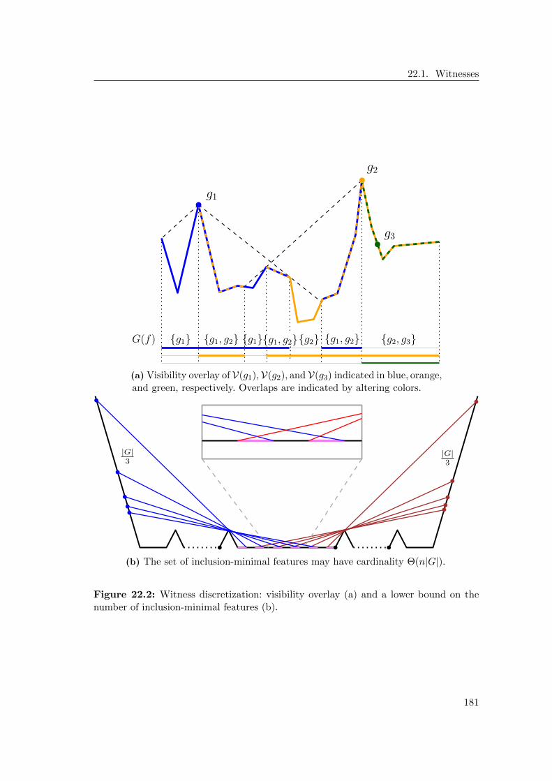
22.1. Witnesses
g1
g2
g1 g1, g2 g1 g2 g1, g2 g2, g3g1, g2
g3
G(f)
(a) Visibility overlay of V(g1),V(g2), and V(g3) indicated in blue, orange,and green, respectively. Overlaps are indicated by altering colors.
|G|3
|G|3
(b) The set of inclusion-minimal features may have cardinality Θ(n|G|).
Figure 22.2: Witness discretization: visibility overlay (a) and a lower bound on thenumber of inclusion-minimal features (b).
181

Chapter 22. Discretization
requires O(n|G|) witnesses, as each guard’s visibility region has O(n) extremal pointswhich bounds the number of features by O(n|G|). However, keeping efficient algorithms inmind, we reduce the number of witnesses, see Section 22.4.3: Similar to the shadow atomicvisibility polygons by Couto et al. [36] — a successful strategy in AGP algorithms [40] —it suffices to include only those features f with inclusion-minimal G(f), i.e., those forwhich no f ′ with G(f ′) ⊂ G(f) exists:
Theorem 22.2. Consider a terrain T and a finite set of guard candidates G withV(G) = T . Let FG denote the set of features of the visibility overlay of G on T andwf ∈ f an arbitrary point in the feature f ∈ FG. Then for
W (G) := wf | f ∈ FG, G(f) is inclusion-minimal , (22.3)
we have that if C ⊆ G is feasible w.r.t. TGP(G,W (G)), then C is also feasible w.r.t.TGP(G,T ) and
OPT(G,W (G)) = OPT(G,T ). (22.4)
Proof. Let C ⊆ G cover W (G) and consider some point w ∈ T . We show that w ∈ V(C).By assumption, w ∈ V(G) and thus w ∈ f for some feature f ∈ FG. The set W (G)contains some witness in wf ∈ f or a witness wf ′ ∈ f ′ with G(f ′) ⊆ G(f) by construction.In the first case, w must be covered, otherwise wf would not be covered and C would beinfeasible for TGP(G,W (G)). In the second case wf ′ is covered, so some guard in G(f ′)is part of C, and that guard also covers f and therefore w.
Regarding Equation (22.4), observe that TGP(G,W (G)) is a relaxation of TGP(G,T ),so OPT(G,W (G)) ≤ OPT(G,T ) follows. Furthermore, if C is feasible and optimalw.r.t. TGP(G,W (G)), it is also feasible for TGP(G,T ) as argued above. It follows that|C| = OPT(G,W (G)) ≥ OPT(G,T ), proving Equation (22.4).
Observation 22.3. Using the set of one witness per inclusion-minimal feature as inEquation (22.3) does not reduce the worst-case complexity of |W (G)| ∈ O(n|G|) witnesses.
Proof. See Figure 22.2(b). For |G| ∈ Θ(n) consider the terrain with Θ(n) valleys with|G|3 guards placed on the left (blue) and the right (red) slope each. In addition there is
one guard (black) placed in each valley. Thus, each of the Θ(n) valleys contains Θ(|G|)inclusion-minimal intervals depicted in violet, resulting in Θ(n|G|) inclusion-minimalfeatures.
Nevertheless, using only inclusion-minimal witnesses significantly speeds up our im-plementation, refer to Section 22.4.3 and Chapter 24.
Observation 22.4. Let p be an endpoint of the visibility overlay of G on T . Then W (G)does not require a witness corresponding to p: p is incident to at least one visibilityinterval I and we have G(p) ⊇ G(I) because visibility regions are closed sets. Hence,G(p) is not inclusion-minimal.
22.2 Guards
Throughout this section, let T be a terrain, V = V (T ) its vertices, and E = E(T ) itsedges. Let C ⊂ T be a finite guard cover of T that is feasible w.r.t. TGP(T, T ) and
182

22.2. Guards
possibly optimal. Define U as all vertices along with the extremal points of their visibilityregions:
U := V ∪⋃v∈Vp | p is extremal in V(v) . (22.5)
Observation 22.5. |U | ∈ O(n2) as noted by Ben-Moshe et al. [18]: It contains nvertices, each associated with O(n) subterrains of at most two extremal points.
Ben-Moshe et al. use a similar set, but they also add an arbitrary point of T betweeneach pair of consecutive points in U . They need these points as witnesses. We, however,keep the witnesses separate by our definition of TGP(G,W ).
In the remainder of this section we show that U contains all guard candidates neces-sary for solving the CTGP, TGP(T, T ), i.e., that OPT(U, T ) = OPT(T, T ). Recall thatOPT(T, T ) ≤ n
2 . Our strategy is to show that in any cover C of T it is always possibleto move a guard in C \ U to a carefully chosen point in U without losing coverage.This procedure preserves the cardinality and feasibility of any feasible cover; iterating itresults in a cover C ⊆ U . In particular, this is possible for an optimal guard cover.
First observe that an edge that is entirely covered by a guard g ∈ C \U is still coveredafter moving g to one of its neighbors in U .
Lemma 22.6. Let g ∈ C \U be a guard that covers an entire edge ei ∈ E, i.e., ei ⊆ V(g).Then u` and ur, the U -neighbors of g, with
u` := maxu ∈ U | u < g (22.6)
ur := minu ∈ U | g < u (22.7)
each entirely cover ei, too, i.e., ei ⊆ V(u`) and ei ⊆ V(ur).
Proof. g covers ei, so vi, vi+1 ∈ V(g), implying g ∈ V(vi) ∩ V(vi+1). Moving g towardsu` does not move g out of V(vi) or V(vi+1), as the boundaries of those regions arecontained in U by construction. Hence, vi, vi+1 ∈ V(u`) and thus ei ⊆ V(u`). Analogously,ei ⊆ V(ur).
It remains to consider the edges not entirely covered by a single guard, refer toFigure 22.3(a). We refer to such edges as critical edges:
Definition 22.7 (Critical Edge). An edge e ∈ E is critical w.r.t. g ∈ C if C \g coverssome part of, but not all of, int(e). If e is critical w.r.t. some g ∈ C we call e a criticaledge.
So e is critical if and only if more than one guard is responsible for covering int(e).
Definition 22.8 (Left-Guard/Right-Guard). g ∈ C is a left-guard (right-guard) ofei ∈ E if g < vi (vi+1 < g) and ei is critical w.r.t. g. We call g a left-guard (right-guard)if it is a left-guard (right-guard) of some e ∈ E.
For the sake of completeness, we state and prove the following lemma which alsofollows from the well-established order claim [18]:
183
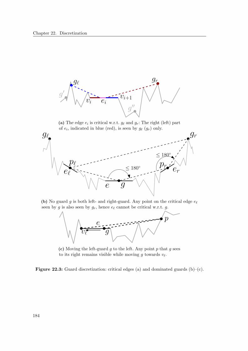
Chapter 22. Discretization
g` gr
g′
g′′ei
vi+1vi
(a) The edge ei is critical w.r.t. g` and gr: The right (left) partof ei, indicated in blue (red), is seen by g` (gr) only.
g
g` gr
e` erp`
≤ 180
≤ 180
pr
e
(b) No guard g is both left- and right-guard. Any point on the critical edge e`seen by g is also seen by gr, hence e` cannot be critical w.r.t. g.
gv`
pe
(c) Moving the left-guard g to the left. Any point p that g seesto its right remains visible while moving g towards v`.
Figure 22.3: Guard discretization: critical edges (a) and dominated guards (b)–(c).
184
22.2. Guards
Lemma 22.9. Let g ∈ C be a guard left of vi (right of vi+1) such that g covers a non-empty subset of int(ei). Then g covers a single interval of ei, including vi+1 (including vi).In particular, this holds if g is a left-guard (right-guard) of ei.
Proof. Refer to Figure 22.3(a), where g` (gr) depicts the guard left of vi (right of vi+1).Obviously, g` is nowhere below the line supporting ei. Let p be a point on ei seen by g`.It follows that g`p and pvi+1 form an x-monotone convex chain that is nowhere below T .Thus, g`vi+1 is nowhere below T . It follows that g` sees vi+1 and any point on pvi+1. Asymmetric argument holds for gr and vi.
Corollary 22.10. For a critical edge there is exactly one left- and exactly one right-guard.
Proof. Suppose for the sake of contradiction that g, g′ ∈ C are distinct critical left-guardsof ei ∈ E. By Lemma 22.9, I := V(g)∩ ei and I ′ := V(g′)∩ ei are connected intervals onei with vi+1 ∈ I, I ′. Assume w.l.o.g. that I ′ ⊆ I. This contradicts g′ being a left-guardof ei because g dominates g′ on ei, i.e., ei ⊆ V(C \ g′). So ei has exactly one criticalleft-guard. A symmetric argument shows that ei has exactly one right-guard.
Corollary 22.11. Let ei ∈ E be a critical edge and let g`, gr ∈ C be its left- andright-guards. Then V(g`) ∩ ei ∩ V(gr) 6= ∅.
Proof. Consider I` := ei∩V(g`). By Lemma 22.9, I` is a single interval on the right of ei,i.e., from some point p` ∈ int(ei) up to its right vertex vi+1. Since ei and V(g`) are closedsets, so is I`, hence, p` is well-defined. Analogously, define Ir := ei ∩ V(gr) and let prbe the rightmost point in Ir. Let pm := 1
2(p` + pr) ∈ ei be the midpoint of the intervalboundaries. We argue in two steps: (1) Observe that I` ∪ Ir = ei. Otherwise, pm /∈ I`, Irwould be covered by some guard g ∈ C \ g`, gr. By Lemma 22.9, g would dominateeither g` or gr on ei, contradicting the precondition that g` and gr are critical w.r.t. ei.(2) Due to ei = I` ∪ Ir, we have pm ∈ I` ∩ Ir. Hence, pm ∈ V(g`) ∩ ei ∩ V(gr) and theclaim follows.
By Lemma 22.6, we can move non-critical guards to one of their neighbors in Ubecause they are only responsible for entire edges. Unfortunately, this is impossible ifg ∈ C \ U is a left- or a right-guard: We might lose coverage of some part of an edgethat is critical w.r.t. g. However, the following lemma establishes that we can move aleft-guard g to its left neighbor vertex if g is not a right-guard (a symmetric version fornon-left-guards follows).
Lemma 22.12. Let C be some finite cover of T , let g ∈ C \ V be a left- but not aright-guard, and let v` := maxv ∈ V | v < g be the rightmost vertex left of g. Then
C ′ = (C \ g) ∪ v` (22.8)
is a guard cover of T .
Proof. Since g is a left-guard of some critical edge er, there is a corresponding right-guard gr of er by Corollary 22.10, see Figure 22.3(b). Let p` ∈ p ∈ V(g) | p ≤ g bea point that g sees to its left. We show that p` is seen by gr: Consider pr, a point in
185

Chapter 22. Discretization
V(g)∩er ∩V(gr), which exists by Corollary 22.11. p`g, gpr, and prgr form a convex chain(convex due to g, pr /∈ V ) that is nowhere below T , so p` ∈ V(gr). Thus, g is dominatedto its left by gr. Moreover, g is dominated to its right by v`, see Figure 22.3(c): Letp ∈ p ∈ V(g) | g ≤ p be a point seen by g located to its right. Then v`g and gp form aconvex chain nowhere below T , so p ∈ V(v`). In conclusion, replacing g by v` in C yieldsa feasible cover because p ∈ V(g) | p ≤ g is covered by gr and p ∈ V(g) | g ≤ pby v`.
Corollary 22.13. Let C be some finite cover of T , let g ∈ C \ V be a right- but noleft-guard, and let vr := minv ∈ V | g < v be the leftmost vertex right of g. Then
C ′ = (C \ g) ∪ vr (22.9)
is a guard cover of T .
So far, the status is that guards in C \U that are neither left- nor right-guard can bemoved to a U -neighbor. Left-guards (right-guards) that are no right-guard (left-guard)can be moved to the next vertex to the left (right). The remaining case, i.e., guards thatare both left- and right-guards, cannot happen:
Lemma 22.14. Let C be a finite cover of T . No g ∈ C \ V is both a left- and aright-guard.
Proof. Refer to Figure 22.3(b). Suppose for the sake of contradiction that g ∈ C \ V isthe left-guard of an edge er (er is to the right of g) and the right-guard of edge e` (e` is tothe left of g). Since er is critical, there must be a right-guard gr of er by Corollary 22.10.By Corollary 22.11 there is a point pr ∈ er seen by g and gr. As g /∈ V , g ∈ int(e) forsome edge e.
Now consider some point p` ∈ V(g) such that p` < g. p` and pr are not below theline supported by e and the same holds for g and gr w.r.t. er. It follows that segmentsp`g, gpr, and prgr form an x-monotone convex chain that is nowhere below T . Hence,p` ∈ V(gr). Since p` was arbitrary, any point p ∈ V(g) to the left of g is also seen by gr,a contradiction to g being a right-guard.
The next theorem shows that the set U as defined in Equation (22.5) contains allguard candidates necessary for a minimum-cardinality guard cover of T .
Theorem 22.15. Let T be a terrain and consider U from Equation (22.5). Then wehave
OPT(U, T ) = OPT(T, T ). (22.10)
Proof. Let C be optimal w.r.t. TGP(T, T ) and observe that C is finite, as placing aguard on every other vertex is feasible. We show how to replace a single guard g ∈ C \Uby one in U while maintaining feasibility, i.e., V(C) = T . The claim then follows byinduction.
Should g be neither left- nor right-guard, it can be replaced by a neighboring pointin U by Lemma 22.6. If g is a left-, but not a right-guard (or vice versa), it can be replacedby its left (right) neighbor in V ⊆ U by Lemma 22.12 (Corollary 22.13). Lemma 22.14asserts that g cannot be a left- and a right-guard at the same time.
186

22.3. Full Discretization
22.3 Full Discretization
We formulate the key result of this chapter: The CTGP, i.e., finding a minimum-cardinality guard cover C guarding an entire terrain T , without any restriction on whereon T the guards can be placed, is a discrete problem with a discretization (U,W (U)) ofsize O(n3) and polynomially bounded coordinate complexity.
Theorem 22.16. Let T be a terrain, and consider U and W (U) from Equations (22.5)and (22.3). Then the following claims hold.
(1) If C ⊆ U is feasible w.r.t. TGP(U,W (U)) then C is feasible w.r.t. TGP(T, T ).Furthermore,
OPT(T, T ) = OPT(U,W (U)). (22.11)
(2) We have |U | ∈ O(n2) and |W (U)| ∈ O(n3).
(3) Let B be the largest number of bits required to represent a coordinate of V . Thenumber of bits required to represent the coordinates of a guard candidate g ∈ U ispolynomial in B.
Proof. To show (1), observe that if C is feasible w.r.t. TGP(U,W (U)), it is feasible w.r.t.TGP(U, T ) by Theorem 22.2; feasibility of C w.r.t. TGP(T, T ) follows from U ⊂ T .Equation (22.11) holds due to
OPT(T, T )(22.10)
= OPT(U, T )(22.4)
= OPT(U,W (U)). (22.12)
Claim (2) follows from Observations 22.5 and 22.3. Regarding (3), observe that if g ∈ V ,the claim trivially holds. Otherwise, g ∈ U \ V is the intersection of two lines, eachspanned by two vertices in V .
22.4 Reducing the Size of the Discretization
While O(n2) guard candidates and O(n3) witnesses, see Theorem 22.16, may be sufficientfrom a theoretical point of view, it is imperative to reduce their numbers for an efficientimplementation. We propose filtering techniques that, while not reducing the asymptoticsize of the discretization, typically remove around 90 % of the guard candidates and aneven larger fraction of the witnesses. The experiments in Chapter 24 demonstrate thisto be a key success factor that increases the size of solvable instances by several ordersof magnitude.
We say that g ∈ T dominates g′ ∈ T if V(g′) ⊆ V(g), in which case g′ can be safelydiscarded. A core issue, however, is that visibility calculations are expensive, so the keychallenge is to identify dominated guard candidates without determining their visibilityregion. The guard filter in Section 22.4.2 is capable of that. We propose guard filters inSections 22.4.1 and 22.4.2, discuss a witness filter in Section 22.4.3, and present an openproblem in Section 22.4.4.
187

Chapter 22. Discretization
e2e3
e4
e5
e6
e7
e1
e2, e3, e4, e5, e6, e7 e1, e2, e3, e4, e5, e6∪e3 ∪e2
∪e7 ∪e1∪e6 ∪e5
Figure 22.4: Edge-interior guards are only responsible for entire edges. Edges can onlybecome visible when crossing some u ∈ U , the arrows indicate in which direction. Onlythe orange regions contain guard candidates that are inclusion-maximal w.r.t. entireedges.
22.4.1 Filtering Dominated Guards
Let T be a terrain and G ⊂ T a finite set of guard candidates with V(G) = T . Considerg, g′ ∈ G, suppose we know V(g) and V(g′), and observe that checking whether g domi-nates g′ takes O(n) time since visibility regions consist of O(n) subterrains. Moreover,removing all dominated guards from G requires O(|G|2) domination queries, i.e., anintolerable O(n5) time when applied to G = U from Equation (22.5).
Instead, we propose a heuristic using O(|G|) domination queries and thus an ac-ceptable O(n3) time for G = U . Suppose G is ordered w.r.t. x-coordinates. The localdomination filter removes all guard candidates that are dominated by one of their neigh-bors. This is based on the observation that neighboring guards’ visibility regions oftenare quite similar or one clearly dominates the other (a local “dent”). Experiments dem-onstrate that this strategy is beneficial in terms of time and memory consumption, seeChapter 24.
22.4.2 Filtering Edge-Interior Guards
Let T be a terrain, U the guard candidates from Equation (22.5), and fix an edge e. ByLemma 22.12, Corollary 22.13, and Lemma 22.14 assume w.l.o.g. that all critical guardsare located at the vertices. Hence, guards in Ue := U ∩ int(e) are only responsible forcovering entire edges. Recall that by construction of U , when moving across u ∈ Ue, avertex becomes visible or invisible, depending on the direction. Furthermore, observethat covering an entire edge is equivalent to seeing both its vertices. The sets of edgesentirely seen by each u ∈ Ue,
Eu := e ∈ E | e ⊆ V(u) = ei ∈ E | vi, vi+1 ∈ V(u), (22.13)
define a partial order on Ue w.r.t. inclusion as indicated in Figure 22.4. Most importantly,u is inclusion-maximal if Eu′ 6⊃ Eu for all u′ ∈ Ue. We show that it suffices to consider
188

22.4. Reducing the Size of the Discretization
the guard candidates that are inclusion-maximal w.r.t. Eu:
Theorem 22.17. Let U ′e ⊆ Ue be the set that only contains inclusion-maximal guardcandidates w.r.t. entire edges, as defined above. Then
U ′ := (U \ Ue) ∪ U ′e (22.14)
admits covering T with the same number of guards as U , i.e.,
OPT(U ′, T ) = OPT(U, T ). (22.15)
Proof. No guard can be a left- and a right-guard at the same time by Lemma 22.14.Furthermore, by Lemma 22.12 (Corollary 22.13), a left-guard (right-guard) can be movedto its left (right) neighbor in V . Thus, w.l.o.g., u ∈ Ue is no left- or right-guard, because Uedoes not contain vertices by definition. Hence, no edge is critical w.r.t. u by Definition 22.7;u is only responsible for covering entire edges and can be replaced by its inclusion-maximalsibling in U ′e without changing the feasibility or cardinality of a cover of T .
The key is that identifying guard candidates u ∈ U \V that are not inclusion-maximalw.r.t. entire edges can be implemented without determining V(u): For each u ∈ U \ V ,store a reference to the vertex whose visibility region is extremal at u, as well as whetherit is situated to the left or to the right of u. This allows to decide which vertex becomesvisible or invisible when sweeping across u from left to right, as indicated in Figure 22.4.
We use the following sweep-line algorithm. For every e ∈ E, sweep through Ue fromleft to right. While encountering u ∈ Ue where new vertices become visible, do nothing.When reaching the first u ∈ Ue where a vertex becomes invisible, report u. Since u isinclusion-maximal w.r.t. vertices, it is inclusion-maximal w.r.t. entire edges. Then ignoreall points corresponding to vertices becoming invisible until encountering the first thatbecomes visible and continue as above. This algorithm reports guard candidates that areinclusion-maximal w.r.t. vertices. However, no vertex can become visible and invisiblein two distinct u, u′ ∈ Ue ⊂ int(e) by Lemma 22.9, hence the reported guard candidatesare inclusion-maximal w.r.t. edges, as claimed.
This efficiently discards up to 98 % of the guard candidates in the CTGP — with-out determining their visibility regions — and essentially removes the computationalboundary between VTGP and CTGP as demonstrated in Chapter 24.
Observation 22.18. The above sweep-line algorithm needs only the visibility regions ofvertices, not those of U \ V . Deciding whether a vertex v becomes visible or invisible atu ∈ Ue depends only on whether u is extremal in V(v) and on v < u, as described above.
Observation 22.19. Filtering U as above still may yield Θ(n2) guard candidates: Inserta vertex below each guard on the slopes in Figure 22.2(b). Then every other interval isinclusion-maximal w.r.t. the vertices on the slopes.
22.4.3 Filtering Witnesses
Let U be a possibly filtered set of guard candidates. The construction of the witnessset W (U) as in Equation (22.3) already includes a filtering mechanism: Only inclusion-minimal witnesses need to be kept. Observe that a smaller, filtered,U automatically yields
189

Chapter 22. Discretization
a smaller W (U). Furthermore, observe that in terms of an implementation witnesses aremuch cheaper then guard candidates: They require no visibility region or coordinates —by Observation 22.1, they only need to store references to the guards covering them.
We acquire witnesses very much like guards in Section 22.4.2: Sort the extremalpoints of all guard candidates’ visibility regions by their x-coordinates. For each of thesepoints we know whether a visibility region opens or closes and to which guard it isassociated. Sweeping through these points, it is straightforward to keep track of whichguard candidates see the current event point and where this set is inclusion-minimal.
Our approach keeps witnesses that are locally, but not necessarily globally, inclusion-minimal. We can efficiently exploit the underlying geometry to identify the locallyinclusion-minimal witnesses, but it is an open question whether globally inclusion-minimalwitnesses can be identified just as efficiently. However, experiments demonstrate thatour approach is extremely effective, see Chapter 24.
22.4.4 Open Problem
Our discretization has size |U |+ |W (U)| ∈ O(n3) by Theorem 22.16. The filters proveinvaluable to our implementation by quickly reducing, on average, the size by morethan 90 % — see Chapter 24 — but do not reduce the asymptotic complexity. In theinterest of finding a small discretization, observe that a discretization that minimizes|G|+ |W | is one where |G| = OPT(T, T ), i.e., just as hard to find as solving TGP(T, T ).Is there a discretization, obtainable in polynomial time, of size o(n3)?
190
CHAPTER 23
NP-Completeness and Approximation
The results in this chapter directly follow from the existence of a polynomially-sizeddiscretization of the CTGP — see Chapter 22 — and are a key motivation for its devel-opment. As as detailed in Chapter 21, our discretization was developed independentlyfrom but after that of King [86], hence, the results in this chapter are implicit to priorwork. Nevertheless, we present them as they are key consequences of Chapter 22.
For a long time, the NP-hardness of the decision variants of the CTGP and the VTGPwere generally assumed but not shown until 2010 by King and Krohn [87].1 The NP-completeness of the decision variant of the VTGP immediately follows. In Theorem 23.1,we establish that the decision version of the CTGP is also a member of NP, and thusNP-complete, which is possible because polynomially many bits suffice to represent allrequired guard coordinates. This is surprising as the more general AGP has been recentlyshown to require irrational guard coordinates [1], even in monotone polygons.
Theorem 23.1. The decision variant of the Continuous Terrain Guarding Problem(CTGP), i.e., the following decision problem is NP-complete:
Input A terrain T with rational vertices V (T ) ⊂ Q2 and k ∈ N.
Output Yes if the CTGP permits k guards G = g1, . . . , gk ⊂ T with V(G) = T , i.e.,if OPT(T, T ) ≤ k, and No otherwise.
Proof. The above problem is known to be NP-hard [87]. It remains to show that it is amember of NP: A non-deterministic Turing machine computes U from Equation (22.5),which is possible in polynomial time by Theorem 22.16, and guesses guards C ⊆ U with|C| ≤ k. It then verifies V(C) = T in polynomial time [75].
Our discretization can be combined with the PTAS for discrete TGP variants byGibson et al. [66].
Theorem 23.2. There exists a PTAS for the Continuous Terrain Guarding Problem(CTGP). That is, for any constant ε > 0, there is a polynomial-time algorithm which,given a terrain T , returns C ⊂ T with V(C) = T and |C| ≤ (1 + ε) OPT(T, T ).
Proof. Using Equations (22.5) and (22.3), we determine the sets U and W (U) for Twith |U |+ |W (U)| ∈ O(n3) in polynomial time by Theorem 22.16. Using the PTAS forTGP(G,W ) with finite G,W ⊂ T by Gibson et al. [66], we compute C ⊆ U ⊂ T with
|C|[66]
≤ (1 + ε) OPT(U,W (U))(22.11)
= (1 + ε) OPT(T, T ) (23.1)
in polynomial time, where C is feasible w.r.t. TGP(T, T ) by Theorem 22.16.
1The conference version of King and Krohn [87] appeared 2010.

Chapter 23. NP-Completeness and Approximation
192

CHAPTER 24
Solver
The discretization and the filters proposed in Chapter 22 allow for an efficient imple-mentation of a solver for the TGP: First determine the guard locations (or start withuser-provided guard candidates when solving a discrete TGP variant), apply the filters,and generate the witnesses. At this point, the problem is a finite instance of SC which canbe solved by an external solver; we use an IP solver. The IP is presented in Section 24.1.We propose the algorithm in Section 24.2. It solves instances of the TGP with up to 106
vertices within roughly 1–2 minutes on a standard desktop computer, as demonstratedin Section 24.3.
Our approach is to efficiently determine and filter a discretization; once the discretiza-tion is obtained, the resulting SC instance is solved by an IP solver. Focusing on thepolynomial-time part of the algorithm and delegating its NP-hard part is founded in ourexperience with the closely related AGP. It has been established that in many AGP-solver variants, the geometric subroutines and not the SC instances form the bottleneckin terms of real-world performance [40]. Finding a discretization and the overhead ofthe EGC paradigm, i.e., the use of exact number types, exhaust computational resourceslong before the SC instances become large enough to be problematic. Furthermore, SCis a well-studied problem and state-of-the-art solvers benefit from that.
We admit that instances deliberately designed to be hard for the underlying IP solverare not covered by the above line of reasoning. Still, we choose to focus on an efficientreduction of TGP to SC instances, as this is required by any fast solver for the TGP.As a consequence, we evaluate our algorithm’s performance in the presence and absenceof the individual filtering techniques. It turns out that these techniques are critical forgood performance.
24.1 IP Formulation
Let T be a terrain and let G,W ⊂ T be finite sets of guard candidates and witnessessuch that W ⊆ V(G). In that case, TGP(G,W ) is an instance of SC:1 We ask for a coverof the set W by a minimal number of subsets from V(g)∩W | g ∈ G. Hence, we obtainthe following IP formulation of TGP(G,W ):
min∑g∈G
xg (24.1)
s.t.∑
g∈V(w)∩G
xg ≥ 1 ∀w ∈W (24.2)
xg ∈ 0, 1 ∀g ∈ G. (24.3)
1Refer to, e.g., Garey and Johnson [63] for a definition of SC.

Chapter 24. Solver
input: Terrain T and mode ∈ VertexGuards,PointGuards . VTGP or CTGPoutput: Guard cover of T
1: U ← V (T ) . vertices are guard candidates in both modes2: W ← ∅3: for each u ∈ U do4: determine V(u)5: end for
6: if PointGuards then . the alternative is VertexGuards7: U ← U ∪⋃v∈Up | p is extremal in V(v) . Equation (22.5)8: if EdgeFilter then9: filter edge-interior guards in U by sweep-line algorithm . Section 22.4.2
10: end if11: for each u ∈ U \ V (T ) do12: determine V(u) . after EdgeFilter, see Section 22.4.213: end for14: end if
15: if DominationFilter then16: filter out guards in U dominated by a neighbor . Section 22.4.117: end if
18: if WitnessFilter then19: W ← inclusion-minimal features of the overlay of U . Equation (22.3)20: else21: W ← all features from the overlay of U . unfiltered Equation (22.3)22: end if
23: solve TGP(U,W ) with an IP solver . Equations (24.1)–(24.3)
Algorithm 24.1: Optimal TGP solutions.
A binary variable xg for each guard candidate g ∈ G indicates whether g is picked: xg = 1if and only if g is part of the cover. For each witness w ∈W , a constraint ensures that wis covered by at least one guard. We minimize the number of guards in the cover. Thisis a standard IP formulation that is, e.g., used in AGP solvers [40].
Choosing G = U (possibly filtered) and W = W (U) from Equations (22.5) and (22.3),(24.1)–(24.3) model the CTGP. In order to solve the VTGP, pick G = V and W = W (V ).For an arbitrary a priori guard discretization G, i.e., for TGP(G,T ), pick W = W (G).
24.2 Algorithm
Algorithm 24.1 has two modes.
(1) PointGuards solves TGP(T, T ) and
(2) VertexGuards solves TGP(V, T ).
194

24.2. Algorithm
Figure 24.1: Exact computations and the Terrain Guarding Problem: The guard candi-date marked by the white circle lies exactly on the intersection of three lines spanned byedges of the terrain. If it is not found due to rounding errors the solution is suboptimal.
Everything except lines 6–14 applies to both modes; lines 6–14 generate non-vertex guardcandidates and possibly filter them. Filtering mechanisms are activated individually:
(1) DominationFilter from Section 22.4.1 removes guard candidates that are domi-nated by one of their neighbors,
(2) EdgeFilter corresponds to the guard filter from Section 22.4.2 and is only appli-cable in the PointGuards mode, and
(3) WitnessFilter determines whether only the inclusion-minimal witness are used,refer to Equation (22.3) and Section 22.4.3.
We remark two things about line 23. (1) It is the only subroutine that may requiresuperpolynomial time, due to the NP-hardness of the TGP [87]. In our experiments,however, this is not the bottleneck of our algorithm; the geometric subroutines requiremost time and memory. We discuss this in Section 24.3.4. (2) Algorithm 24.1 transformsan instance of VTGP or CTGP into an instance of SC which it delegates to a solver.An IP or SAT solver, an SC approximation algorithm, the PTAS by Gibson et al. [66],or any other solver (including those oblivious to the underlying geometry) can be usedas a drop-in replacement. Observe that all solvers benefit from our filtering framework.However, since benchmarking the underlying solver is not our concern, we restrict ourexperiments to a state-of-the-art IP solver.
24.2.1 Implementation
We implemented Algorithm 24.1 in C++11 and compiled with g++-4.8.4 [64]. Thegeometric subroutines use CGAL-4.6 [28] (the Computational Geometry AlgorithmsLibrary) with the visibility implementation of Haas and Hemmer [70] and we solveIPs using CPLEX-12.6.0 [37]. Furthermore, we use boost-1.58.0 [23] and simple-svg-1.0.0 [126].
Like CGAL, our implementation adheres to the EGC paradigm, compare, e.g., Pionand Fabri [121]. In a nutshell, this means that no geometric subroutine introducesrounding errors. As an illustration of why this is necessary consider the terrain T inFigure 24.1.2 There is exactly one optimal solution of TGP(T, T ) and it requires the
2We use T as a test case of our software.
195
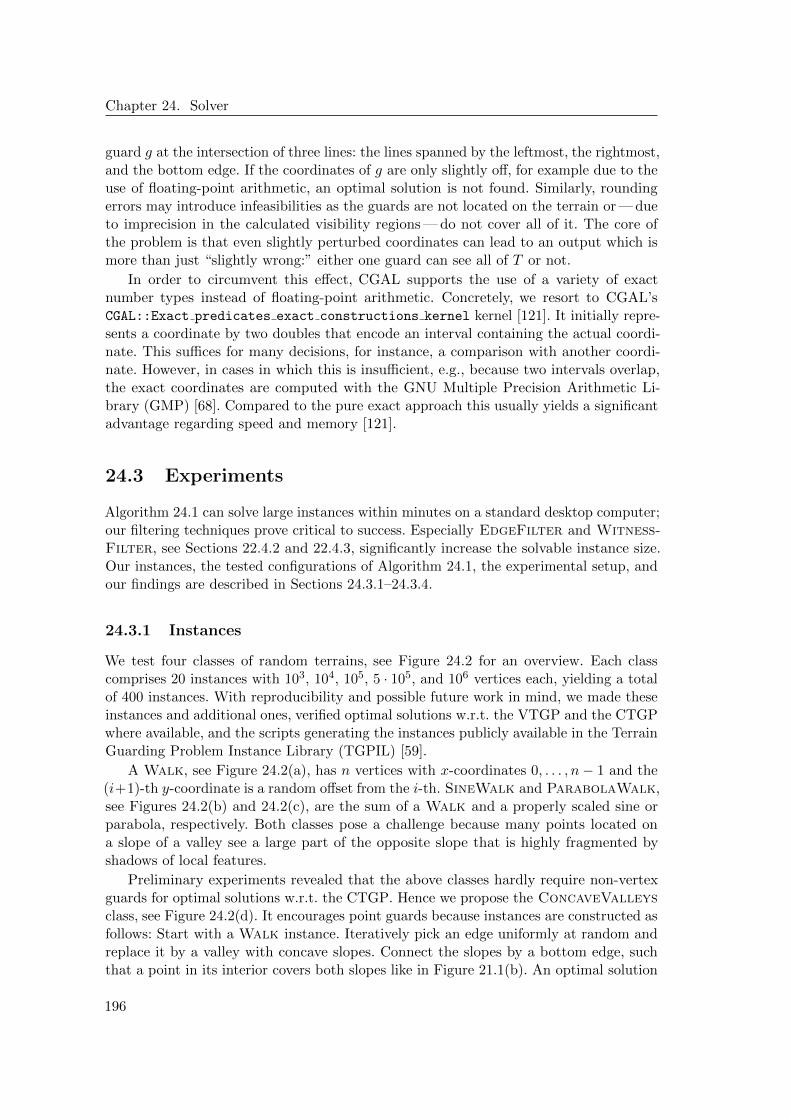
Chapter 24. Solver
guard g at the intersection of three lines: the lines spanned by the leftmost, the rightmost,and the bottom edge. If the coordinates of g are only slightly off, for example due to theuse of floating-point arithmetic, an optimal solution is not found. Similarly, roundingerrors may introduce infeasibilities as the guards are not located on the terrain or — dueto imprecision in the calculated visibility regions — do not cover all of it. The core ofthe problem is that even slightly perturbed coordinates can lead to an output which ismore than just “slightly wrong:” either one guard can see all of T or not.
In order to circumvent this effect, CGAL supports the use of a variety of exactnumber types instead of floating-point arithmetic. Concretely, we resort to CGAL’sCGAL::Exact predicates exact constructions kernel kernel [121]. It initially repre-sents a coordinate by two doubles that encode an interval containing the actual coordi-nate. This suffices for many decisions, for instance, a comparison with another coordi-nate. However, in cases in which this is insufficient, e.g., because two intervals overlap,the exact coordinates are computed with the GNU Multiple Precision Arithmetic Li-brary (GMP) [68]. Compared to the pure exact approach this usually yields a significantadvantage regarding speed and memory [121].
24.3 Experiments
Algorithm 24.1 can solve large instances within minutes on a standard desktop computer;our filtering techniques prove critical to success. Especially EdgeFilter and Witness-Filter, see Sections 22.4.2 and 22.4.3, significantly increase the solvable instance size.Our instances, the tested configurations of Algorithm 24.1, the experimental setup, andour findings are described in Sections 24.3.1–24.3.4.
24.3.1 Instances
We test four classes of random terrains, see Figure 24.2 for an overview. Each classcomprises 20 instances with 103, 104, 105, 5 · 105, and 106 vertices each, yielding a totalof 400 instances. With reproducibility and possible future work in mind, we made theseinstances and additional ones, verified optimal solutions w.r.t. the VTGP and the CTGPwhere available, and the scripts generating the instances publicly available in the TerrainGuarding Problem Instance Library (TGPIL) [59].
A Walk, see Figure 24.2(a), has n vertices with x-coordinates 0, . . . , n− 1 and the(i+1)-th y-coordinate is a random offset from the i-th. SineWalk and ParabolaWalk,see Figures 24.2(b) and 24.2(c), are the sum of a Walk and a properly scaled sine orparabola, respectively. Both classes pose a challenge because many points located ona slope of a valley see a large part of the opposite slope that is highly fragmented byshadows of local features.
Preliminary experiments revealed that the above classes hardly require non-vertexguards for optimal solutions w.r.t. the CTGP. Hence we propose the ConcaveValleysclass, see Figure 24.2(d). It encourages point guards because instances are constructed asfollows: Start with a Walk instance. Iteratively pick an edge uniformly at random andreplace it by a valley with concave slopes. Connect the slopes by a bottom edge, suchthat a point in its interior covers both slopes like in Figure 21.1(b). An optimal solution
196

24.3. Experiments
(a) Walk: Random walk with uniform step width.
(b) SineWalk: Sum of a sine wave and a random walk.
(c) ParabolaWalk: Sum of a parabolaand a random walk.
(d) ConcaveValleys: Optimal solu-tions require point guards in the valleys.
Figure 24.2: Four classes of random test instances available in the TGPIL [59].
197

Chapter 24. Solver
Configuration Mode EdgeFilter DominationFilter WitnessFilter
VDefault VertexGuards n/a yes yesVNoDom VertexGuards n/a no yesVNoW VertexGuards n/a yes no
PDefault PointGuards yes yes yesPNoEdge PointGuards no yes yesPNoDom PointGuards yes no yesPNoW PointGuards yes yes no
Table 24.1: Algorithm configurations, VTGP above and CTGP below.
w.r.t. the CTGP for such a terrain usually requires at least one guard in a bottom edge’sinterior.
None of the above classes deliberately provokes the NP-hardness of the TGP; theyare not designed to contain a reduction of hard instances of, e.g., PLANAR 3SAT, asused in the NP-hardness proof of King and Krohn [87]. As motivated above, testing suchinstances is out of scope: We provide and evaluate the means to transform a terrain intoa small discretization that can be handed to a solver; IP, PTAS, SAT, or other. Thetransformation has to be efficient and our experiments are designed to test just that.Combinatorially hard instances merely benchmark the underlying solver.
24.3.2 Configurations
We test Algorithm 24.1 in seven configurations, see Table 24.1, to individually assess theimpact of each filtering technique from Section 22.4. VDefault, VNoDom, and VNoWtest the VertexGuards mode; PDefault, PNoEdge, PNoDom, and PNoW testthe considerably harder PointGuards mode. Recall that EdgeFilter does not applyto VertexGuards mode. Since we test 400 instances, this results in 2800 test runs.
24.3.3 Experimental Setup
We used eight identical Linux 3.13 machines with Intel Core i7-3770 CPUs running at3.4 GHz, provided with 8 MB of cache and 16 GB of main memory. Every run was limitedto 15 minutes of CPU time and 14 GB of memory. Our software, except solving IPs withCPLEX, is not parallelized. Refer to Section 24.2.1 for details regarding the toolchainand the implementation.
24.3.4 Results
The solution rate and median CPU time of every combination of configuration, instanceclass, and instance complexity are listed in Tables 24.2 and 24.3; each cell correspondsto 20 test runs. Due to the imposed time and memory limits, not all test runs succeeded;we account for unfinished test runs with an infinite completion time. Hence, we use themedian instead of the mean throughout the analysis. More detailed timing informationis presented in Figure 24.5.
198

24.3. Experiments
Configuration Instance#vertices
103 104 105 5 · 105 106
VDefault
Walk 100 % 100 % 100 % 100 % 100 %SineWalk 100 % 100 % 100 % 0 % 0 %ParabolaWalk 100 % 100 % 100 % 0 % 0 %ConcaveValleys 100 % 100 % 100 % 100 % 100 %
VNoDom
Walk 100 % 100 % 100 % 100 % 100 %SineWalk 100 % 100 % 100 % 0 % 0 %ParabolaWalk 100 % 100 % 100 % 0 % 0 %ConcaveValleys 100 % 100 % 100 % 100 % 100 %
VNoW
Walk 100 % 100 % 100 % 0 % 0 %SineWalk 100 % 100 % 0 % 0 % 0 %ParabolaWalk 100 % 25 % 0 % 0 % 0 %ConcaveValleys 100 % 100 % 100 % 0 % 0 %
PDefault
Walk 100 % 100 % 100 % 100 % 100 %SineWalk 100 % 100 % 100 % 0 % 0 %ParabolaWalk 100 % 100 % 100 % 0 % 0 %ConcaveValleys 100 % 100 % 100 % 100 % 100 %
PNoEdge
Walk 100 % 100 % 100 % 55 % 0 %SineWalk 100 % 100 % 0 % 0 % 0 %ParabolaWalk 100 % 100 % 0 % 0 % 0 %ConcaveValleys 100 % 100 % 100 % 90 % 0 %
PNoDom
Walk 100 % 100 % 100 % 100 % 100 %SineWalk 100 % 100 % 100 % 0 % 0 %ParabolaWalk 100 % 100 % 100 % 0 % 0 %ConcaveValleys 100 % 100 % 100 % 100 % 100 %
PNoW
Walk 100 % 100 % 100 % 0 % 0 %SineWalk 100 % 100 % 0 % 0 % 0 %ParabolaWalk 100 % 20 % 0 % 0 % 0 %ConcaveValleys 100 % 100 % 100 % 0 % 0 %
Table 24.2: Solution rate by configuration, instance class, and instance complexity. Eachcell corresponds to 20 test runs.
Except in PNoEdge mode, all unsolved instances were caused by running out ofmemory, we discuss this phenomenon below. In the following, we turn our attention tothe relative hardness of the instance classes, an overview of VertexGuards and Point-Guards modes, the impact of EdgeFilter, DominationFilter and WitnessFilter,timing behavior, and memory consumption.
Overview: Instances Tables 24.2 and 24.3 clearly reveal that the SineWalk andParabolaWalk instances are harder to solve than their Walk and ConcaveValleyscounterparts. This is to be expected, since SineWalk and ParabolaWalk contain aWalk as additive noise and since the sole purpose of ConcaveValleys is to encourageplacing non-vertex guards, see Section 24.3.1. Furthermore, SineWalk and Parabola-Walk comprise facing valleys, resulting in highly fragmented visibility regions andcomplex visibility overlays in which a large portion of the guards and witnesses cannotbe filtered out. This induces time and memory intensive calculations and a complex IP,
199

Chapter 24. Solver
Configuration Instance#vertices
103 104 105 5 · 105 106
VDefault
Walk 0.0 s 0.2 s 2.9 s 18.0 s 40.3 sSineWalk 0.0 s 0.9 s 13.8 s n/a n/aParabolaWalk 0.1 s 1.8 s 21.7 s n/a n/aConcaveValleys 0.2 s 2.4 s 24.2 s 177.2 s 337.6 s
VNoDom
Walk 0.0 s 0.3 s 3.6 s 21.8 s 48.6 sSineWalk 0.1 s 1.3 s 18.2 s n/a n/aParabolaWalk 0.1 s 2.5 s 27.8 s n/a n/aConcaveValleys 0.2 s 2.4 s 24.3 s 177.1 s 411.0 s
VNoW
Walk 0.0 s 0.4 s 8.8 s n/a n/aSineWalk 0.1 s 6.4 s n/a n/a n/aParabolaWalk 0.4 s n/a n/a n/a n/aConcaveValleys 0.2 s 2.7 s 32.0 s n/a n/a
PDefault
Walk 0.0 s 0.3 s 4.6 s 27.9 s 62.4 sSineWalk 0.1 s 1.7 s 26.3 s n/a n/aParabolaWalk 0.2 s 3.3 s 45.1 s n/a n/aConcaveValleys 0.1 s 0.8 s 10.3 s 68.2 s 137.4 s
PNoEdge
Walk 0.2 s 4.5 s 79.7 s 833.3 s n/aSineWalk 1.0 s 58.8 s n/a n/a n/aParabolaWalk 4.1 s 220.3 s n/a n/a n/aConcaveValleys 0.2 s 3.2 s 58.3 s 652.3 s n/a
PNoDom
Walk 0.0 s 0.4 s 5.0 s 31.5 s 70.4 sSineWalk 0.1 s 2.0 s 31.1 s n/a n/aParabolaWalk 0.2 s 4.0 s 51.8 s n/a n/aConcaveValleys 0.1 s 0.9 s 10.7 s 68.0 s 145.5 s
PNoW
Walk 0.0 s 0.6 s 10.4 s n/a n/aSineWalk 0.1 s 7.8 s n/a n/a n/aParabolaWalk 0.6 s n/a n/a n/a n/aConcaveValleys 0.1 s 1.1 s 20.8 s n/a n/a
Table 24.3: Median CPU time by configuration, instance class, and instance complexity.Each cell corresponds to 20 test runs.
200
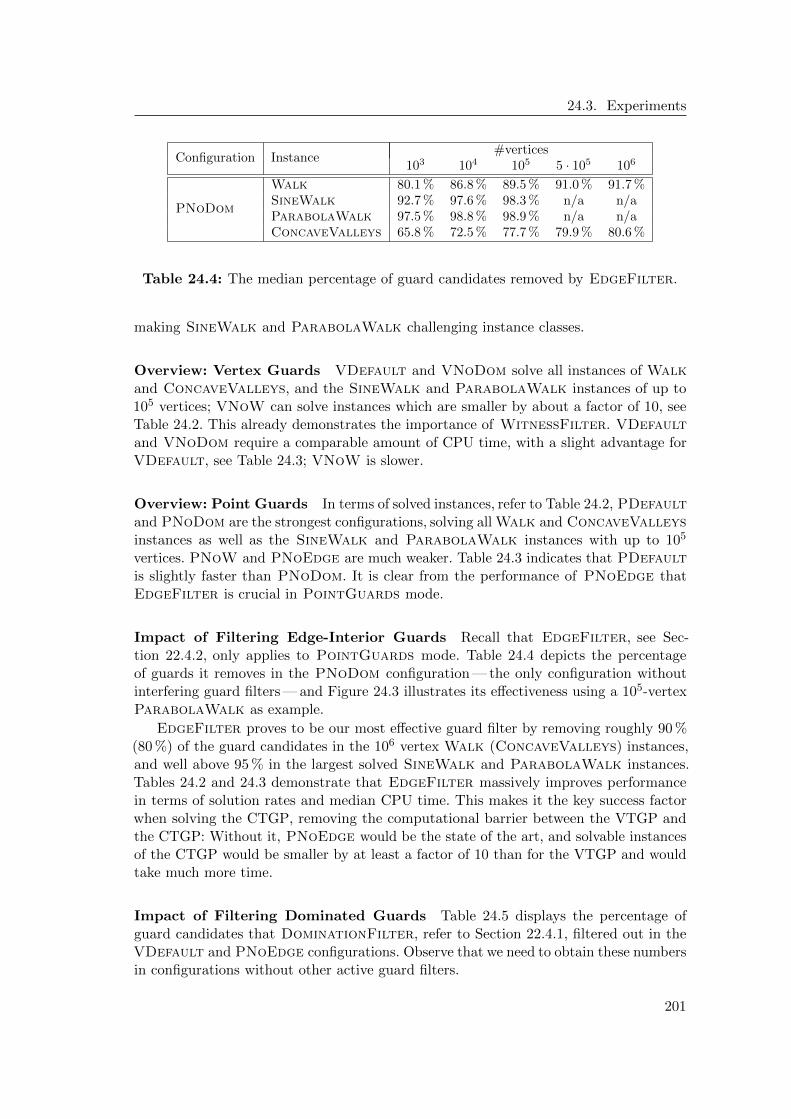
24.3. Experiments
Configuration Instance#vertices
103 104 105 5 · 105 106
PNoDom
Walk 80.1 % 86.8 % 89.5 % 91.0 % 91.7 %SineWalk 92.7 % 97.6 % 98.3 % n/a n/aParabolaWalk 97.5 % 98.8 % 98.9 % n/a n/aConcaveValleys 65.8 % 72.5 % 77.7 % 79.9 % 80.6 %
Table 24.4: The median percentage of guard candidates removed by EdgeFilter.
making SineWalk and ParabolaWalk challenging instance classes.
Overview: Vertex Guards VDefault and VNoDom solve all instances of Walkand ConcaveValleys, and the SineWalk and ParabolaWalk instances of up to105 vertices; VNoW can solve instances which are smaller by about a factor of 10, seeTable 24.2. This already demonstrates the importance of WitnessFilter. VDefaultand VNoDom require a comparable amount of CPU time, with a slight advantage forVDefault, see Table 24.3; VNoW is slower.
Overview: Point Guards In terms of solved instances, refer to Table 24.2, PDefaultand PNoDom are the strongest configurations, solving all Walk and ConcaveValleysinstances as well as the SineWalk and ParabolaWalk instances with up to 105
vertices. PNoW and PNoEdge are much weaker. Table 24.3 indicates that PDefaultis slightly faster than PNoDom. It is clear from the performance of PNoEdge thatEdgeFilter is crucial in PointGuards mode.
Impact of Filtering Edge-Interior Guards Recall that EdgeFilter, see Sec-tion 22.4.2, only applies to PointGuards mode. Table 24.4 depicts the percentageof guards it removes in the PNoDom configuration — the only configuration withoutinterfering guard filters — and Figure 24.3 illustrates its effectiveness using a 105-vertexParabolaWalk as example.
EdgeFilter proves to be our most effective guard filter by removing roughly 90 %(80 %) of the guard candidates in the 106 vertex Walk (ConcaveValleys) instances,and well above 95 % in the largest solved SineWalk and ParabolaWalk instances.Tables 24.2 and 24.3 demonstrate that EdgeFilter massively improves performancein terms of solution rates and median CPU time. This makes it the key success factorwhen solving the CTGP, removing the computational barrier between the VTGP andthe CTGP: Without it, PNoEdge would be the state of the art, and solvable instancesof the CTGP would be smaller by at least a factor of 10 than for the VTGP and wouldtake much more time.
Impact of Filtering Dominated Guards Table 24.5 displays the percentage ofguard candidates that DominationFilter, refer to Section 22.4.1, filtered out in theVDefault and PNoEdge configurations. Observe that we need to obtain these numbersin configurations without other active guard filters.
201

Chapter 24. Solver
(a) Unfiltered guard candidates. (b) Filtered guard candidates.
Figure 24.3: The effect of EdgeFilter (excerpt of the right slope of a 105-vertexParabolaWalk). Circles depict guard candidates. Local features on the right slope(e.g., the left peak) can induce many guard candidates (e.g., on the right): A featurecasts a slightly different shadow for each vertex on the left slope (not depicted), resultingin many guard candidates. EdgeFilter mitigates this effect very well.
Configuration Instance#vertices
103 104 105 5 · 105 106
VDefault
Walk 65.8 % 64.1 % 63.6 % 63.5 % 63.5 %SineWalk 58.5 % 63.0 % 63.6 % n/a n/aParabolaWalk 59.9 % 63.3 % 63.6 % n/a n/aConcaveValleys 13.4 % 13.1 % 13.3 % 13.3 % 13.3 %
PNoEdge
Walk 92.9 % 94.7 % 95.6 % 95.8 % n/aSineWalk 88.1 % 96.7 % n/a n/a n/aParabolaWalk 93.2 % 98.0 % n/a n/a n/aConcaveValleys 77.1 % 80.5 % 83.9 % 85.0 % n/a
Table 24.5: Median percentage of guard candidates removed by DominationFilter.
202

24.3. Experiments
Configuration Instance#vertices
103 104 105 5 · 105 106
VDefault
Walk 91.9 % 94.3 % 95.4 % 96.1 % 96.4 %SineWalk 95.8 % 98.8 % 99.3 % n/a n/aParabolaWalk 98.6 % 99.4 % 99.5 % n/a n/aConcaveValleys 76.5 % 80.5 % 83.7 % 85.1 % 85.5 %
PDefault
Walk 91.9 % 94.3 % 95.5 % 96.1 % 96.4 %SineWalk 96.3 % 98.9 % 99.3 % n/a n/aParabolaWalk 98.7 % 99.5 % 99.5 % n/a n/aConcaveValleys 80.3 % 84.2 % 87.4 % 88.7 % 89.1 %
Table 24.6: Median percentage of witnesses removed by WitnessFilter.
DominationFilter has no impact on the solution rates within the limits imposed byour setup (see Section 24.3.3). VDefault and PDefault are slightly faster than VNo-Dom and PNoDom, respectively. The key advantage of DominationFilter, however,is that it saves memory by deleting dominated guard candidates; this is important sincememory consumption is the bottleneck of our implementation, see below.
Impact of Filtering Witnesses The percentage of witnesses removed by Witness-Filter, see Section 22.4.3, in the VDefault and PDefault configurations is displayedin Table 24.6. Throughout our instances, WitnessFilter removes the vast majority ofwitnesses, often more than 95 %. Furthermore, Table 24.2 clearly shows that disabling itreduces the solvable instance size by at least a factor of 10. Given that PointGuardsmode may have to deal with |W (U)| ∈ Θ(n3) witnesses, this is not surprising. All of thisrenders WitnessFilter simple, fast, and useful.
Timing Behavior Figures 24.4 and 24.5 show how much CPU time is spent in eachpart of Algorithm 24.1 and the distribution of the CPU time, respectively. For a compar-ison, we pick an instance class and a complexity that was solved by every configuration,a Walk with 105 vertices, the other combinations are omitted as they permit the sameinterpretation.
The strongest impact is that of EdgeFilter, which is disabled in the rightmostbar in Figure 24.4. Without EdgeFilter there is a computational gap between Point-Guards and VertexGuards mode, as determining visibility regions of unneededguards dominates the CPU time. Guard-filtering time also increases in PNoEdge modebecause DominationFilter is active and has more guards to compare.
WitnessFilter has the second most important impact. In its absence, CPU timeroughly doubles due to an increased IP solution time: In the IP, non-inclusion-minimalwitnesses form constraints that are dominated by the inclusion-minimal witnesses’ con-straints. The IP solver eliminates dominated constraints in a preprocessing phase, butWitnessFilter does so more efficiently, since it exploits the underlying geometry.
The timing behavior is hardly influenced by DominationFilter. It is, however,beneficial w.r.t. memory consumption, see below.
A general observation is that the filtering mechanisms significantly reduce the com-
203

Chapter 24. Solver
VDefault VNoDom VNoW PDefault PNoDom PNoW PNoEdge0
10
20
30
40
50
60
70
80
90
tim
e [
s]
walk, n=100000
VisibilityGuard FiltersIPOther
Figure 24.4: Median CPU time by subroutine regarding 105-vertex Walk instances.
204
24.3. Experiments
VDefault VNoDom VNoW PDefault PNoDom PNoW PNoEdge0
50
100
150
200
tim
e [
s]
walk, n=100000
Figure 24.5: Box plot of CPU time regarding 105-vertex Walk instances. Boxes depict1st–3rd quartile, whiskers the 10th and 90th percentile.
205

Chapter 24. Solver
putational overhead. One would expect the IP solution-time to dominate an exact solverfor an NP-hard problem. This, however, tends not to be the case in geometric optimiza-tion problems like the AGP and its relatives [40], an effect that is rooted in the EGCparadigm: Instead of floating-point arithmetic, exact number types must be used toensure consistent and correct results. VDefault and PDefault still are not clearlydominated by the IP solution time, but much closer to it than unfiltered approaches.
Memory Consumption Within our experimental setup, using the VDefault andPDefault modes, even instances with 106 vertices are solved within minutes. All un-solved configuration–instance pairs run out of memory, not time. The only exception isPNoEdge, which occasionally runs out of time owed to the large number of unnecessaryvisibility calculations otherwise prevented by EdgeFilter, see Table 24.4 and the corre-sponding discussion. So as long as instances are not designed to reveal the NP-hardnessof the TGP, the limiting resource is memory.
Two phases of Algorithm 24.1 generate a significant amount of data that persistsin memory. One phase is the computation of all visibility regions of all vertices V inline 4. This may store Θ(n2) x-coordinates3 in memory which define the unfilteredguard-candidate set U . Filters remove the vast majority of candidates from U . Theother phase is the one that determines the visibility regions of the remaining pointsin U \ V , generating the largest chunk of data in line 12: At this point, we may keepΘ(n3) x-coordinates in memory. It is not obvious how to avoid holding all these visibilityregions in memory since a guard at the far right of the terrain may still see a regionat its very left; it is an open question if it is possible to apply WitnessFilter beforeknowing all extremal points.
We remark that the memory bottleneck may be amplified by the fact that we followthe EGC paradigm, compare Section 24.2.1, which ensures a correct and consistent rep-resentation of all visibility regions and a correct order of all visibility events. Specifically,we do not store coordinates of points using floating-point arithmetic. In our case, theCGAL::Exact predicates exact constructions kernel kernel [121] performed betterin terms of CPU time and memory usage than non-lazy variants like GMP [68].
3We never store y-coordinates of visibility regions. Instead, we represent them as unions of intervalsof x-coordinates.
206

CHAPTER 25
Conclusion
We present a discretization with O(n2) guard candidates and O(n3) witnesses for theCTGP. It was discovered independently from that of King [86] and is asymptoticallysmaller by a factor of n. This positively answers King’s question whether O(n2) guardcandidates suffice. The existence of a polynomially sized discretization settles two openquestions: (1) The decision variant of the CTGP is a member of NP and, since itsNP-hardness is known [87], NP-complete. (2) Moreover, the CTGP admits a PTAS, sincethe PTAS for the discrete TGP [66] applies to our discretization.
Furthermore, we propose an algorithm for finding optimal solutions for the CTGP andthe VTGP; it directly generalizes to other discrete versions of the TGP. Our implemen-tation solves instances with up to 106 vertices within minutes. The filtering techniquesreducing the size of the discretization — and with it the geometric overhead — are a keysuccess factor, essentially removing the computational barrier between the CTGP andthe VTGP.

Chapter 25. Conclusion
208

List of Figures
“Their art was the art that convinced — when we saw the pictures we saw thedaemons themselves and were afraid of them.”
H. P. Lovecraft, Pickman’s Model
3.1 Separation of Concerns . . . . . . . . . . . . . . . . . . . . . . . . . . . . 15
4.1 Generic Synchronous State Machine . . . . . . . . . . . . . . . . . . . . 224.2 Registers . . . . . . . . . . . . . . . . . . . . . . . . . . . . . . . . . . . . 234.3 Masking Register . . . . . . . . . . . . . . . . . . . . . . . . . . . . . . . 244.4 Combinational Logic DAG . . . . . . . . . . . . . . . . . . . . . . . . . . 274.5 Behavior of Combinational Logic DAGs . . . . . . . . . . . . . . . . . . 274.6 Executions . . . . . . . . . . . . . . . . . . . . . . . . . . . . . . . . . . 32
5.1 Pivotal Sequence . . . . . . . . . . . . . . . . . . . . . . . . . . . . . . . 38
6.1 Gate-Level Multiplexers . . . . . . . . . . . . . . . . . . . . . . . . . . . 446.2 Metastability Propagation in Multiplexers . . . . . . . . . . . . . . . . . 456.3 CMOS Inverter . . . . . . . . . . . . . . . . . . . . . . . . . . . . . . . . 486.4 Transistor-Level Multiplexers . . . . . . . . . . . . . . . . . . . . . . . . 496.5 Metastability-Containing 4-Valued Multiplexer . . . . . . . . . . . . . . 51
8.1 Unrolling . . . . . . . . . . . . . . . . . . . . . . . . . . . . . . . . . . . 568.2 Masking-Register Simulation . . . . . . . . . . . . . . . . . . . . . . . . 58
9.1 Karnaugh Map of a Multiplexer . . . . . . . . . . . . . . . . . . . . . . . 63
10.1 Time-to-Digital Converter . . . . . . . . . . . . . . . . . . . . . . . . . . 6910.2 Binary Reflected Gray Code . . . . . . . . . . . . . . . . . . . . . . . . . 72
17.1 FRT Tree . . . . . . . . . . . . . . . . . . . . . . . . . . . . . . . . . . . 137
21.1 The Terrain Guarding Problem . . . . . . . . . . . . . . . . . . . . . . . 174
22.1 Witness Visibility Kernel . . . . . . . . . . . . . . . . . . . . . . . . . . 17922.2 Witness Discretization . . . . . . . . . . . . . . . . . . . . . . . . . . . . 18122.3 Guard Discretization . . . . . . . . . . . . . . . . . . . . . . . . . . . . . 18422.4 Filtering Edge-Interior Guards . . . . . . . . . . . . . . . . . . . . . . . 188
24.1 Exact Computations . . . . . . . . . . . . . . . . . . . . . . . . . . . . . 19524.2 Instances . . . . . . . . . . . . . . . . . . . . . . . . . . . . . . . . . . . 19724.3 The Effect of EdgeFilter . . . . . . . . . . . . . . . . . . . . . . . . . 20224.4 CPU Time by Subroutine . . . . . . . . . . . . . . . . . . . . . . . . . . 204

List of Figures
24.5 CPU Time Boxplot . . . . . . . . . . . . . . . . . . . . . . . . . . . . . . 205
210

List of Tables
“Ich seh’ Gauß. . . ”
Matthias Fugger
4.1 Gate Behavior under Metastability . . . . . . . . . . . . . . . . . . . . . 26
6.1 Metastability-Containing Multiplexers in Sorting Networks . . . . . . . 52
24.1 Configurations . . . . . . . . . . . . . . . . . . . . . . . . . . . . . . . . 19824.2 Solution Rate . . . . . . . . . . . . . . . . . . . . . . . . . . . . . . . . . 19924.3 CPU Time . . . . . . . . . . . . . . . . . . . . . . . . . . . . . . . . . . 20024.4 EdgeFilter . . . . . . . . . . . . . . . . . . . . . . . . . . . . . . . . . 20124.5 DominationFilter . . . . . . . . . . . . . . . . . . . . . . . . . . . . . 20224.6 WitnessFilter . . . . . . . . . . . . . . . . . . . . . . . . . . . . . . . 203

List of Tables
212

List of Algorithms
“Beware of bugs in the above code; I have only proved it correct, not tried it.”
Donald Knuth
6.1 Metastability-Containing Multiplexer . . . . . . . . . . . . . . . . . . . . 46
13.1 Moore-Bellman-Ford Algorithm . . . . . . . . . . . . . . . . . . . . . . . 9413.2 Dijkstra’s Algorithm . . . . . . . . . . . . . . . . . . . . . . . . . . . . . 94
15.1 Oracle for MBF-like Algorithms . . . . . . . . . . . . . . . . . . . . . . . 125
17.1 FRT Embedding via LE Lists . . . . . . . . . . . . . . . . . . . . . . . . 139
24.1 TGP Solver . . . . . . . . . . . . . . . . . . . . . . . . . . . . . . . . . . 194

List of Algorithms
214

List of Acronyms
“Abbrv. is the abbrv. for abbrv.”
unknown
3SAT Boolean 3-Satisfiability Problem [63]
ADC Analog-to-Digital Converter
AGP Art Gallery Problem [117]
APSP All-Pairs Shortest Paths (Example 14.6)
APWP All-Pairs Widest Paths (Example 14.15)
ASIC Application-Specific Integrated Circuit
BFS Breadth-First Search
BRGC Binary Reflected Gray Code (Section 10.2)
CGAL Computational Geometry Algorithms Library [28]
CMOS Complementary Metal-Oxide-Semiconductor [4, 131]
CMUX Metastability-Containing Multiplexer (Equation (6.5))
CRCW Concurrent Read Concurrent Write [77]
CREW Concurrent Read Exclusive Write [77]
CTGP Continuous Terrain Guarding Problem (Definition 21.1)
DAG Directed Acyclic Graph
DCO Digitally Controlled Oscillator
DNF Disjunctive Normal Form
EGC Exact Geometric Computation [121]
EREW Exclusive Read Exclusive Write [77]
FET Field-Effect Transistor [4, 131]
FPGA Field-Programmable Gate Array [131]
FRT Fakcharoenphol, Rao, and Talwar [50] (Definition 17.2)
FPT Fixed-Parameter Tractable
GMP GNU Multiple Precision Arithmetic Library [68]
ID Identifier
IP Integer Linear Program
k-DSDP k-Distinct-Shortest Distance Problem (Definition 14.22)
k-SDP k-Shortest Distance Problem (Definition 14.22)

List of Acronyms
k-SSP k-Source Shortest Paths (Example 14.5)
LE Least Element (Equation (17.11))
LP Linear Program
MBF Moore-Bellman-Ford [16, 54, 116] (Algorithm 13.1)
MBF-like Moore-Bellman-Ford-like (Definition 13.11)
MSSP Multi-Source Shortest Paths (Example 14.7)
MST Minimum Spanning Tree
MSWP Multi-Source Widest Paths (Example 14.16)
MTBF Mean Time Between Failures
MUX Multiplexer (Equation (6.2))
PRAM Parallel Random-Access Machine [77]
PTAS Polynomial-Time Approximation Scheme
SAT Boolean Satisfiability Problem [63]
SC Set Cover [63]
SLF Simple Linear Function (Definition 13.13)
SPD Shortest-Path Diameter (Equation (12.10))
SPICE Simulation Program with Integrated Circuit Emphasis [127]
SSSP Single-Source Shortest Paths (Example 14.4)
SSWP Single-Source Widest Paths (Example 14.14)
TC Thermometer Code (Section 10.2)
TDC Time-to-Digital Converter
TGP Terrain Guarding Problem (Definition 21.1)
TGPIL Terrain Guarding Problem Instance Library [59]
TSP Traveling Salesman Problem [63]
TTP Time-Triggered Protocol
VLSI Very Large-Scale Integration
VTGP Terrain Guarding Problem with Vertex Guards (Definition 21.1)
WPP Widest Path Problem (Section 14.2)
216

Bibliography
“Quotations — the karaoke of ideas.”
John Oliver, Last Week Tonight
[1] M. Abrahamsen, A. Adamaszek, and T. Miltzow. Irrational guards are sometimesneeded. CoRR, abs/1701.05475, 2017.
[2] P. K. Agarwal and M. Sharir. Arrangements and their applications. In J.-R.Sack and J. Urrutia, editors, Handbook of Computational Geometry, pages 49–119.North-Holland, Amsterdam, first edition, 2000.
[3] M. Ajtai, J. Komlos, and E. Szemeredi. An O(n log n) sorting network. In Pro-ceedings of the 15th Annual ACM Symposium on Theory of Computing (STOC),pages 1–9, 1983.
[4] P. E. Allen and D. R. Holberg. CMOS Analog Circuit Design. The Oxford Series inElectrical and Computer Engineering. Oxford University Press USA, third edition,2011.
[5] N. Alon, Z. Galil, and O. Margalit. On the exponent of the all pairs shortest pathproblem. Journal of Computer and System Science, 54(2):255–262, 1997.
[6] N. Alon, R. M. Karp, D. Peleg, and D. B. West. A graph-theoretic game and itsapplication to the k-server problem. SIAM Journal on Computing, 24(1):78–100,1995.
[7] B. Awerbuch and Y. Azar. Buy-at-bulk network design. In Proceedings of the 38thAnnual Symposium on Foundations of Computer Science (FOCS), pages 542–547,1997.
[8] Y. Bartal. Probabilistic approximation of metric spaces and its algorithmic applica-tions. In Proceedings of the 37th Annual Symposium on Foundations of ComputerScience (FOCS), pages 184–193, 1996.
[9] Y. Bartal. On approximating arbitrary metrices by tree metrics. In Proceedingsof the 30th Annual ACM Symposium on Theory of Computing (STOC), pages161–168, 1998.
[10] S. Baswana and S. Sen. A simple and linear time randomized algorithm forcomputing sparse spanners in weighted graphs. Random Structures & Algorithms,30(4):532–563, 2007.
[11] K. E. Batcher. Sorting networks and their applications. In American Federationof Information Processing Societies (AFIPS), pages 307–314, 1968.
Bibliography
[12] R. Becker, A. Karrenbauer, S. Krinninger, and C. Lenzen. Near-optimal approxi-mate shortest paths and transshipment in distributed and streaming models. CoRR,abs/1607.05127, 2016.
[13] S. Beer and R. Ginosar. Eleven ways to boost your synchronizer. IEEE Transactionson VLSI Systems, 23(6):1040–1049, 2015.
[14] S. Beer, R. Ginosar, J. Cox, T. Chaney, and D. M. Zar. Metastability challengesfor 65nm and beyond: simulation and measurements. In Design, Automation andTest in Europe (DATE), pages 1297–1302, 2013.
[15] S. Beer, R. Ginosar, M. Priel, R. R. Dobkin, and A. Kolodny. The devolution ofsynchronizers. In 16th IEEE International Symposium on Asynchronous Circuitsand Systems (ASYNC), pages 94–103, 2010.
[16] R. E. Bellman. On a routing problem. Quarterly Applied Mathematics, 16:87–90,1958.
[17] R. Belschner, J. Berwanger, F. Bogenberger, C. Ebner, H. Eisele, B. Elend, T. M.Forest, T. Fuhrer, P. Fuhrmann, F. Hartwich, et al. FlexRay communicationprotocol, 2003. Patent Application EP2002/0008171.
[18] B. Ben-Moshe, M. J. Katz, and J. S. B. Mitchell. A constant-factor approxima-tion algorithm for optimal 1.5d terrain guarding. SIAM Journal on Computing,36(6):1631–1647, 2007.
[19] G. E. Blelloch, Y. Gu, J. Shun, and Y. Sun. Parallelism in randomized incremen-tal algorithms. In Proceedings of the 28th ACM Symposium on Parallelism inAlgorithms and Architectures (SPAA), pages 467–478, 2016.
[20] G. E. Blelloch, Y. Gu, and Y. Sun. Efficient construction of probabilistic treeembeddings. CoRR, abs/1605.04651, 2016.
[21] G. E. Blelloch, A. Gupta, and K. Tangwongsan. Parallel probabilistic tree em-beddings, k-median, and buy-at-bulk network design. In Proceedings of the 24thACM Symposium on Parallelism in Algorithms and Architectures (SPAA), pages205–213, 2012.
[22] G. E. Blelloch and K. Tangwongsan. Parallel approximation algorithms for facility-location problems. In Proceedings of the 22nd ACM Symposium on Parallelism inAlgorithms and Architectures (SPAA), pages 315–324, 2010.
[23] boost C++ libraries. http://www.boost.org/.
[24] J. A. Brzozowski, Z. Esik, and Y. Iland. Algebras for hazard detection. In 31stIEEE International Symposium on Multiple-Valued Logic (ISMVL), pages 3–12,2001.
[25] J. A. Brzozowski and M. Yoeli. On a ternary model of gate networks. IEEETransactions on Computers, C-28(3):178–184, March 1979.
218

Bibliography
[26] J. Bund, C. Lenzen, and M. Medina. Near-optimal metastability-containing sortingnetworks. In Design, Automation and Test in Europe (DATE), pages 226–231, 2017.
[27] F. Bungiu, M. Hemmer, J. Hershberger, K. Huang, and A. Kroller. Efficientcomputation of visibility polygons. CoRR, abs/1403.3905, 2014.
[28] The computational geometry algorithms library (CGAL). http://www.cgal.org/.
[29] A. K. Chandra and G. Markowsky. On the number of prime implicants. DiscreteMathematics, 24(1):7–11, 1978.
[30] V. Chvatal. A combinatorial theorem in plane geometry. Journal of CombinatorialTheory, Series B, 18(1):39–41, 1975.
[31] K. Chwa, B. Jo, C. Knauer, E. Moet, R. van Oostrum, and C. Shin. Guarding artgalleries by guarding witnesses. International Journal of Computational Geometry& Applications, 16(2-3):205–226, 2006.
[32] K. L. Clarkson and K. R. Varadarajan. Improved approximation algorithms forgeometric set cover. Discrete & Computational Geometry, 37(1):43–58, 2007.
[33] E. Cohen. Size-estimation framework with applications to transitive closure andreachability. Journal of Computer and System Sciences, 55(3):441–453, 1997.
[34] E. Cohen. Polylog-time and near-linear work approximation scheme for undirectedshortest paths. Journal of the ACM, 47(1):132–166, 2000.
[35] T. H. Cormen, C. E. Leiserson, R. L. Rivest, and C. Stein. Introduction to Algo-rithms. MIT Press, third edition, 2009.
[36] M. C. Couto, P. J. de Rezende, and C. C. de Souza. An exact algorithm for mini-mizing vertex guards on art galleries. International Transactions in OperationalResearch, 18(4):425–448, 2011.
[37] IBM ILOG CPLEX Optimization Studio. http://www.ibm.com/software/
integration/optimization/cplex-optimizer/.
[38] A. Das Sarma, S. Holzer, L. Kor, A. Korman, D. Nanongkai, G. Pandurangan,D. Peleg, and R. Wattenhofer. Distributed verification and hardness of distributedapproximation. SIAM Journal on Computing, 41(5):1235–1265, 2012.
[39] V. De Heyn, G. Van der Plas, J. Ryckaert, and J. Craninckx. A fast start-up 3GHz–10GHz digitally controlled oscillator for UWB impulse radio in 90nm CMOS. InEuropean Solid State Circuits Conference, pages 484–487, September 2007.
[40] P. J. de Rezende, C. C. de Souza, S. Friedrichs, M. Hemmer, A. Kroller, and D. C.Tozoni. Engineering art galleries. In Algorithm Engineering – Selected Resultsand Surveys, volume 9220 of Lecture Notes in Computer Science, pages 379–417.Springer, 2016.
[41] E. W. Dijkstra. A note on two problems in connexion with graphs. NumerischeMathematik, 1(1):269–271, 1959.
219

Bibliography
[42] S. Durocher, P. C. Li, and S. Mehrabi. Guarding orthogonal terrains. In Proceedingsof the 27th Canadian Conference on Computational Geometry (CCCG), 2015.
[43] E. B. Eichelberger. Hazard detection in combinational and sequential switchingcircuits. IBM Journal of Research and Development, 9(2):90–99, March 1965.
[44] S. Eidenbenz. Approximation algorithms for terrain guarding. Information Pro-cessing Letters, 82(2):99–105, 2002.
[45] S. Eidenbenz, C. Stamm, and P. Widmayer. Inapproximability results for guardingpolygons and terrains. Algorithmica, 31(1):79–113, 2001.
[46] K. M. Elbassioni, E. Krohn, D. Matijevic, J. Mestre, and D. Severdija. Improvedapproximations for guarding 1.5-dimensional terrains. Algorithmica, 60(2):451–463,2011.
[47] M. Elkin. An unconditional lower bound on the time-approximation trade-off forthe distributed minimum spanning tree problem. SIAM Journal on Computing,36(2):433–456, 2006.
[48] M. Elkin and O. Neiman. Hopsets with constant hopbound, and applications toapproximate shortest paths. In Proceedings of the 57th Annual Symposium onFoundations of Computer Science (FOCS), pages 128–137, 2016.
[49] M. Ernestus, S. Friedrichs, M. Hemmer, J. Kokemuller, A. Kroller, M. Moeini, andC. Schmidt. Algorithms for art gallery illumination. Journal Global Optimization,68(1):23–45, 2017.
[50] J. Fakcharoenphol, S. Rao, and K. Talwar. A tight bound on approximatingarbitrary metrics by tree metrics. Journal of Computer and System Sciences,69(3):485–497, 2004.
[51] S. P. Fekete, S. Friedrichs, A. Kroller, and C. Schmidt. Facets for art galleryproblems. Algorithmica, 73(2):411–440, 2015.
[52] M. J. Fischer, N. A. Lynch, and M. Paterson. Impossibility of distributed consensuswith one faulty process. Journal of the ACM, 32(2):374–382, 1985.
[53] S. Fisk. A short proof of Chvatal’s watchman theorem. Journal of CombinatorialTheory, Series B, 24(3):374, 1978.
[54] L. R. Ford. Network flow theory. Technical report, The RAND Corporation, 1956.
[55] S. Friedrichs, M. Fugger, and C. Lenzen. Metastability-containing circuits. CoRR,abs/1606.06570, 2016.
[56] S. Friedrichs, M. Hemmer, J. King, and C. Schmidt. The continuous 1.5d ter-rain guarding problem: Discretization, optimal solutions, and PTAS. Journal ofComputational Geometry, 7(1):256–284, 2016.
220

Bibliography
[57] S. Friedrichs, M. Hemmer, and C. Schmidt. A PTAS for the continuous 1.5dterrain guarding problem. In Proceedings of the 26th Canadian Conference onComputational Geometry (CCCG), pages 367–373, 2014.
[58] S. Friedrichs, M. Hemmer, and C. Schmidt. Exact solutions for the continuousterrain guarding problem. In 31st European Workshop on Computational Geometry(EuroCG), pages 212–215, 2015.
[59] S. Friedrichs, M. Hemmer, and C. Schmidt. Terrain guarding problem instancelibrary. http://resources.mpi-inf.mpg.de/tgp/index.html#instances, Au-gust 2015. Version 2015-08-06.
[60] S. Friedrichs and A. Kinali. Efficient metastability-containing multiplexers. InIEEE Computer Society Annual Symposium on VLSI (ISVLSI), 2017. To appear.
[61] S. Friedrichs and C. Lenzen. Parallel metric tree embedding based on an algebraicview on Moore-Bellman-Ford. In Proceedings of the 28th ACM Symposium onParallelism in Algorithms and Architectures (SPAA), pages 455–466, 2016.
[62] M. Fugger, A. Kinali, C. Lenzen, and T. Polzer. Metastability-aware memory-efficient time-to-digital converters. In 23rd IEEE International Symposium onAsynchronous Circuits and Systems (ASYNC), 2017.
[63] M. R. Garey and D. S. Johnson. Computers and Intractability: A Guide to theTheory of NP-Completeness. W. H. Freeman, 1979.
[64] The GNU compiler collection. http://gcc.gnu.org/.
[65] M. Ghaffari and C. Lenzen. Near-optimal distributed tree embedding. In Pro-ceedings of the 28th International Symposium on Distributed Computing (DISC),pages 197–211, 2014.
[66] M. Gibson, G. Kanade, E. Krohn, and K. R. Varadarajan. Guarding terrains vialocal search. Journal of Computational Geometry, 5(1):168–178, 2014.
[67] R. Ginosar. Fourteen ways to fool your synchronizer. In 9th IEEE InternationalSymposium on Asynchronous Circuits and Systems (ASYNC), pages 89–97, 2003.
[68] The GNU multiple precision arthmetic library. https://gmplib.org/.
[69] C. T. Gray, W. Liu, W. A. M. Van Noije, T. A. Hughes, and R. K. Cavin. Asampling technique and its CMOS implementation with 1Gb/s bandwidth and25ps resolution. IEEE Journal of Solid-State Circuits, 29(3):340–349, 1994.
[70] A. Haas and M. Hemmer. Efficient algorithms and implementations for visibility in1.5d terrains. In 31st European Workshop on Computational Geometry (EuroCG),pages 216–219, 2015.
[71] M. Hauptmann and M. Karpinski. A compendium on Steiner tree problems. http://theory.cs.uni-bonn.de/info5/steinerkompendium/netcompendium.html,2015. Visited 2017-04-25.
221
Bibliography
[72] U. Hebisch and H. J. Weinert. Semirings: Algebraic Theory and Applications inComputer Science. Series in algebra. World Scientific, 1998.
[73] M. Henzinger, S. Krinninger, and D. Nanongkai. A deterministic almost-tightdistributed algorithm for approximating single-source shortest paths. In Proceed-ings of the 48th Annual ACM Symposium on Theory of Computing (STOC), pages489–498, 2016.
[74] D. A. Huffman. The design and use of hazard-free switching networks. Journal ofthe ACM, 4(1):47–62, January 1957.
[75] F. Hurtado, M. Loffler, I. Matos, V. Sacristan, M. Saumell, R. I. Silveira, andF. Staals. Terrain visibility with multiple viewpoints. International Journal ofComputational Geometry & Applications, 24(4):275–306, 2014.
[76] International technology roadmap for semiconductors. http://www.itrs2.net/,2013.
[77] J. JaJa. An Introduction to Parallel Algorithms. Addison-Wesley, 1992.
[78] D. S. Johnson. A catalog of complexity classes. In Handbook of TheoreticalComputer Science, Volume A: Algorithms and Complexity, pages 67–161. Elsevier,1990.
[79] J. Kahn, M. Klawe, and D. Kleitman. Traditional art galleries require fewerwatchmen. SIAM Journal on Algebraic and Discrete Methods, 4(2):194–206, 1983.
[80] M. J. Katz and G. S. Roisman. On guarding the vertices of rectilinear domains.International Journal of Computational Geometry & Applications, 39(3):219–228,2008.
[81] M. Khan, F. Kuhn, D. Malkhi, G. Pandurangan, and K. Talwar. Efficient dis-tributed approximation algorithms via probabilistic tree embeddings. DistributedComputing, 25(3):189–205, 2012.
[82] F. Khodakarami, F. Didehvar, and A. Mohades. A fixed-parameter algorithm forguarding 1.5d terrains. Theoretical Computer Science, 595:130–142, 2015.
[83] A. Kinali, F. Huemer, and C. Lenzen. Fault-tolerant clock synchronization withhigh precision. In IEEE Computer Society Annual Symposium on VLSI (ISVLSI),pages 490–495, 2016.
[84] J. King. Errata on “A 4-approximation for guarding 1.5-dimensional terrains”.http://www.cs.mcgill.ca/~jking/papers/4apx_latin.pdf. Visited 2017-06-05.
[85] J. King. A 4-approximation algorithm for guarding 1.5-dimensional terrains. In7th Latin American Theoretical Informatics Symposium (LATIN), pages 629–640,2006.
[86] J. King. Guarding Problems and Geometric Split Trees. PhD thesis, McGillUniversity, 2010.
222

Bibliography
[87] J. King and E. Krohn. Terrain guarding is NP-hard. SIAM Journal on Computing,40(5):1316–1339, 2011.
[88] D. J. Kinniment. Synchronization and Arbitration in Digital Systems. Wiley, 2008.
[89] D. J. Kinniment, A. Bystrov, and A. V. Yakovlev. Synchronization circuit perfor-mance. IEEE Journal of Solid-State Circuits, 37(2):202–209, February 2002.
[90] S. C. Kleene. Introduction to Metamathematics. Van Nostrand, 1952.
[91] P. N. Klein and S. Subramanian. A randomized parallel algorithm for single-sourceshortest paths. Journal of Algorithms, 25(2):205–220, 1997.
[92] H. Kopetz and G. Bauer. The time-triggered architecture. Proceedings of theIEEE, 91(1):112–126, 2003.
[93] H. Kopetz, A. Kruger, D. Millinger, and A. V. Schedl. A synchronization strategyfor a time-triggered multicluster real-time system. In 14th Symposium on ReliableDistributed Systems (SRDS), pages 154–161, 1995.
[94] H. Kopetz and W. Ochsenreiter. Clock synchronization in distributed real-timesystems. IEEE Transactions on Computers, 36(8):933–940, 1987.
[95] A. Kroller, T. Baumgartner, S. P. Fekete, and C. Schmidt. Exact solutions andbounds for general art gallery problems. ACM Journal of Experimental Algorith-mics, 17(2):2.3:1–2.3:23, 2012.
[96] L. Lamport, R. E. Shostak, and M. C. Pease. The Byzantine generals problem.ACM Transactions on Programming Languages and Systems, 4(3):382–401, 1982.
[97] A. Laurentini. Guarding the walls of an art gallery. The Visual Computer, 15(6):265–278, 1999.
[98] D. Lee and A. K. Lin. Computational complexity of art gallery problems. IEEETransactions on Information Theory, 32(2):276–282, 1986.
[99] C. Lenzen, M. Fugger, A. Kinali, S. Friedrichs, and M. Medina. Efficientand dependable clock synchronization in hardware, 2016. Patent ApplicationPCT/EP2016/002179.
[100] C. Lenzen and M. Medina. Efficient metastability-containing Gray code 2-sort.In 22nd IEEE International Symposium on Asynchronous Circuits and Systems(ASYNC), pages 49–56, 2016.
[101] C. Lenzen and B. Patt-Shamir. Fast routing table construction using small mes-sages: extended abstract. In Proceedings of the 46th Annual ACM Symposium onTheory of Computing (STOC), pages 381–390, 2013.
[102] C. Lenzen and B. Patt-Shamir. Improved distributed Steiner forest construction.In Proceedings of the ACM Symposium on Principles of Distributed Computing(PODC), pages 262–271, 2014.
223

Bibliography
[103] C. Lenzen and B. Patt-Shamir. Fast partial distance estimation and applications.In Proceedings of the ACM Symposium on Principles of Distributed Computing(PODC), pages 153–162, 2015.
[104] C. Lenzen and D. Peleg. Efficient distributed source detection with limited band-width. In Proceedings of the ACM Symposium on Principles of Distributed Com-puting (PODC), pages 375–382, 2013.
[105] A. Lumsdaine, D. P. Gregor, B. Hendrickson, and J. W. Berry. Challenges inparallel graph processing. Parallel Processing Letters, 17(1):5–20, 2007.
[106] J. Lundelius Welch and N. A. Lynch. A new fault-tolerant algorithm for clocksynchronization. Information and Computation, 77(1):1–36, 1988.
[107] N. A. Lynch. Distributed Algorithms. Morgan Kaufmann, 1996.
[108] L. R. Marino. General theory of metastable operation. IEEE Transactions onComputers, 30(2):107–115, February 1981.
[109] G. Martinovic, D. Matijevic, and D. Severdija. Efficient parallel implementationsof approximation algorithms for guarding 1.5d terrains. Croatian OperationalResearch Review, 6(1):79–89, 2015.
[110] M. Mendel and C. Schwob. Fast C-K-R partitions of sparse graphs. ChicagoJournal of Theoretical Computer Science, 2009(2):1–18, 2009.
[111] M. Mendler, T. R. Shiple, and G. Berry. Constructive Boolean circuits and theexactness of timed ternary simulation. Formal Methods in System Design, 40(3):283–329, 2012.
[112] R. R. Mettu and C. G. Plaxton. Optimal time bounds for approximate clustering.Machine Learning, 56(1-3):35–60, 2004.
[113] U. Meyer and P. Sanders. ∆-stepping: a parallelizable shortest path algorithm.Journal of Algorithms, 49(1):114–152, 2003.
[114] M. Mitzenmacher and E. Upfal. Probability and Computing: Randomized Algo-rithms and Probabilistic Analysis. Cambridge University Press, 2005.
[115] M. Mohri. Semiring frameworks and algorithms for shortest-distance problems.Journal of Automata, Languages and Combinatorics, 7(3):321–350, 2002.
[116] E. F. Moore. The shortest path through a maze. In Symposium on the Theory ofSwitching, pages 87–90, 1959.
[117] J. O’Rourke. Art Gallery Theorems and Algorithms. International Series of Mono-graphs on Computer Science. Oxford University Press, New York, 1987.
[118] J. O’Rourke and K. J. Supowit. Some NP-hard polygon decomposition problems.IEEE Transactions on Information Theory, 29(2):181–189, 1983.
224

Bibliography
[119] D. Peleg. Distributed Computing: A Locality-Sensitive Approach. SIAM, Philadel-phia, 2000.
[120] D. Peleg and V. Rubinovich. A near-tight lower bound on the time complexityof distributed minimum-weight spanning tree construction. SIAM Journal onComputing, 30(5):1427–1442, 2000.
[121] S. Pion and A. Fabri. A generic lazy evaluation scheme for exact geometriccomputations. Science of Computer Programming, 76(4):307–323, 2011.
[122] T. E. Rahkonen and J. T. Kostamovaara. The use of stabilized CMOS delay linesfor the digitization of short time intervals. IEEE Journal of Solid-State Circuits,28(8):887–894, 1993.
[123] G. W. Roberts and M. Ali-Bakhshian. A brief introduction to time-to-digital anddigital-to-time converters. IEEE Transactions on Circuits and Systems, 57(3):153–157, 2010.
[124] D. Schuchardt and H. Hecker. Two NP-hard art-gallery problems for ortho-polygons. Mathematical Logic Quarterly, 41:261–267, 1995.
[125] T. C. Shermer. Recent results in art galleries. Proceedings of the IEEE, 80(9):1384–1399, 1992.
[126] simple-svg. http://code.google.com/p/simple-svg/.
[127] Simulation program with integrated circuit emphasis (SPICE). http://ngspice.sourceforge.net/.
[128] G. Tarawneh, M. Fugger, and C. Lenzen. Metastability tolerant computing. In 23rdIEEE International Symposium on Asynchronous Circuits and Systems (ASYNC),2017.
[129] G. Tarawneh and A. V. Yakovlev. An RTL method for hiding clock domain crossinglatency. In IEEE International Conference on Electronics, Circuits and Systems(ICECS), pages 540–543, 2012.
[130] G. Tarawneh, A. V. Yakovlev, and T. S. T. Mak. Eliminating synchronizationlatency using sequenced latching. IEEE Transactions on VLSI Systems, 22(2):408–419, 2014.
[131] U. Tietze, C. Schenk, and E. Gamm. Halbleiter-Schaltungstechnik. Springer Vieweg,fifteenth edition, 2012.
[132] S. H. Unger. Hazards and delays in asynchronous sequential switching circuits.IRE Transactions on Circuit Theory, 6(1):12–25, Mar 1959.
[133] H. J. M. Veendrick. The behaviour of flip-flops used as synchronizers and predictionof their failure rate. IEEE Journal of Solid-State Circuits, 15(2):169–176, 1980.
225

Bibliography
[134] A. V. Yakovlev, M. Kishinevsky, A. Kondratyev, and L. Lavagno. OR causality:Modelling and hardware implementation. In 15th International Conference onApplication and Theory of Petri Nets, pages 568–587, 1994.
[135] U. Zwick. All pairs shortest paths using bridging sets and rectangular matrixmultiplication. Journal of the ACM, 49(3):289–317, 2002.
226