methodology development for passive component reliability ... reports/fy 2011/11-3030 neup... ·...
TRANSCRIPT

Methodology Development for Passive Component Reliability
Modeling in a Multi-Physics Simulation Environment
Reactor Concepts Dr. Tunc Aldemir
The Ohio State University
In collaboration with: Pacific Northwest National Laboratory
Rich Reister, Federal POC Curtis Smith, Technical POC
Project No. 11-3030

i
FINAL REPORT
Project Title: 3030: Methodology Development for Passive Component Reliability Modeling in a Multi-Physics Simulation Environment (LWRS-2: Risk-Informed Safety Margin Characterization)
Date of Report: December 31, 2014 Recipient: The Ohio State University
154 West 12th Avenue Columbus, Ohio, 43210
Contract Number:
42898 30
Principal Investigator:
Tunc Aldemir, (614) 292-4627, [email protected]
Collaborators: R. Denning, [email protected] (The Ohio State University) Umit Catalyurek, [email protected] (The Ohio State University) S. Unwin, [email protected] (Pacific Northwest National Laboratory)
Abstract: Reduction in safety margin can be expected as passive structures and components undergo degradation with time. Limitations in the traditional probabilistic risk assessment (PRA) methodology constrain its value as an effective tool to address the impact of aging effects on risk and for quantifying the impact of aging management strategies in maintaining safety margins. A methodology has been developed to address multiple aging mechanisms involving large numbers of components (with possibly statistically dependent failures) within the PRA framework in a computationally feasible manner when the sequencing of events is conditioned on the physical conditions predicted in a simulation environment, such as the New Generation System Code (NGSC) concept. Both epistemic and aleatory uncertainties can be accounted for within the same phenomenological framework and maintenance can be accounted for in a coherent fashion. The framework accommodates the prospective impacts of various intervention strategies such as testing, maintenance, and refurbishment. The methodology is illustrated with several examples.
NEUP 11-3030 Final Report 12/31/2014
ii
TABLE OF CONTENTS List of Figures ................................................................................................................................................ iii
List of Tables ................................................................................................................................................ iv
1. Introduction ............................................................................................................................................. 1
2. The Paradigm ......................................................................................................................................... 2
3. Passive Component Selection ................................................................................................................ 5
4. Physics Based Aging Degradation Models Under Consideration .......................................................... 5
4.1 State Transition SCC Model ................................................................................................... 5
4.2 The Parametric Scott Model for SCC of SG Tubes [11] ...................................................... 11
4.3 The KWU-KR Model to describe FAC Driven Degradation [12]........................................... 13
5. Incorporation of Maintenance Activities into the Paradigm .................................................................. 15
5.1 Probabilistic Treatment of Steam Generator Tube Failure .................................................. 16
5.2 Modeling Repair/Replacement Action in the PRA ............................................................... 18
6. Example Implementations .................................................................................................................... 18
6.1 Impact of Local Conditions on Transition Rates .................................................................. 18
6.2 Sensitivity of Transition Rates to Uncertainties .................................................................... 22
6.3 Aging and Maintenance Impacts on a SLB/MSLIV/SGTR Scenario .................................... 34
7. Conclusion and Recommendations for Future Work ............................................................................ 34
8. References ........................................................................................................................................... 36
APPENDIX A: The MATLAB Graphical User Interface Aging_GUI.m and Related Functions ................... 39
APPENDIX B: Surveillance And Detection Of Crack Precursors ............................................................... 62
.................................................................................................................................................................... 72
NEUP 11-3030 Final Report 12/31/2014
iii
List of Figures Figure 2.1: The Paradigm ............................................................................................................................. 4 Figure 4.1: State Transition Model for Multi-State Degradation Process [10] ............................................. 6 Figure 4.2: Comparison of the semi-Markov model to the results reported in [10] ................................... 10 Figure 4.3: Main window of the GUI ......................................................................................................... 12 Figure 4.4: Degradation mechanisms responsible for SG tube plugging over the years ............................ 12 Figure 6.1: RELAP 5 nodalization of the PWR: (a) plant, b) SG and pressurizer ...................................... 20 Figure 6.2: Comparison of the state transition model results using: (a) Table 4.1 data, (b) RELAP5 temperature/pressure data for a 4 loop Generic PWR pressurizer surge line pipe weld (Alloy 182) ......... 22 Figure 6.3: Schematic illustration of the uncertainty analysis performed with LHS for sampling size 5 and for two parameters: temperature (T) and residual weld stress (σ) have normal distributions. .................... 25 Figure 6.4: Structure of Agingso_LHS ....................................................................................................... 25 Figure 6.5: Rupture and Leak State Probabilities during 80 years in case of 100 realizations of LHS for T ∼ Normal (344.9, 0.0882), σ∼ Normal (300.3, 110). .................................................................................. 26 Figure 6.6: Rupture and Leak State Probabilities during 80 years in case of 100 realizations of LHS for 27 Figure 6.7: Rupture and Leak State Probabilities during 80 years in case of 100 realizations of LHS for T=618 K, σ∼ Normal (300.3, 110) .............................................................................................................. 27 Figure 6.8: Rupture and Leak State Probabilities during 80 years in case of 100 realizations of LHS for 28 Figure 6.9: Leak and Rupture State Probabilities during 80 years in case of 100 realizations of LHS for 29 Figure 6.10: Rupture State Probabilities, stress and temperature realizations at t=10, 40 and 80 years in case of 100 realizations of LHS for T ∼ Normal (617.9, 0.0882), σ∼ Normal (300.3, 110) ....................... 30 Figure 6.11: Rupture State Probabilities, stress and temperature realizations at t=40 and 60 years in case of 100 realizations of LHS for T ∼ Normal (617.9, 0.0882), σ∼ Normal (300.3, 110) ............................. 30 Figure 6.12: Rupture probability change as a function of temperature (T) and weld stress (σ) at 40 years. .................................................................................................................................................................... 32 Figure 6.13: Illustration of single step and two-step LHS comparisons ..................................................... 33 Figure 6.14: Comparison of single-step and two-step LHS results ............................................................ 34

NEUP 11-3030 Final Report 12/31/2014
iv
List of Tables Table 4.1: Keller’s Geometric factor, kc, in Eq. (4.14) (adapted from [4]) ................................................ 14 Table 6.1: Temperature dependent model input parameters for crack initiation and growth rate in Eqs.(4.3)-(4.8) for Alloy 182 ...................................................................................................................... 19 Table 6.2: Definition of the inputs in Eq.(4.7) and their values used in different studies .......................... 23 Table 6.3: Definition of the Inputs in Eq. (4.8) and Their Values used in Different Studies .................... 24 Table 6.4: Fitting equation coefficients with 95% confidence bounds ....................................................... 31 Table 6.5: Statistic goodness-of-fit data ..................................................................................................... 31
1
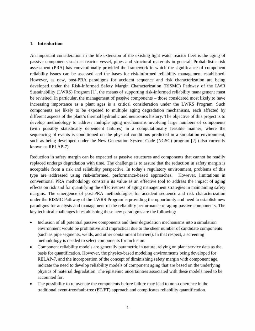
1. Introduction An important consideration in the life extension of the existing light water reactor fleet is the aging of passive components such as reactor vessel, pipes and structural materials in general. Probabilistic risk assessment (PRA) has conventionally provided the framework in which the significance of component reliability issues can be assessed and the bases for risk-informed reliability management established. However, as new, post-PRA paradigms for accident sequence and risk characterization are being developed under the Risk-Informed Safety Margin Characterization (RISMC) Pathway of the LWR Sustainability (LWRS) Program [1], the means of supporting risk-informed reliability management must be revisited. In particular, the management of passive components – those considered most likely to have increasing importance as a plant ages is a critical consideration under the LWRS Program. Such components are likely to be exposed to multiple aging degradation mechanisms, each affected by different aspects of the plant’s thermal hydraulic and neutronics history. The objective of this project is to develop methodology to address multiple aging mechanisms involving large numbers of components (with possibly statistically dependent failures) in a computationally feasible manner, where the sequencing of events is conditioned on the physical conditions predicted in a simulation environment, such as being developed under the New Generation System Code (NGSC) program [2] (also currently known as RELAP-7).
Reduction in safety margin can be expected as passive structures and components that cannot be readily replaced undergo degradation with time. The challenge is to assure that the reduction in safety margin is acceptable from a risk and reliability perspective. In today’s regulatory environment, problems of this type are addressed using risk-informed, performance-based approaches. However, limitations in conventional PRA methodology constrain its value as an effective tool to address the impact of aging effects on risk and for quantifying the effectiveness of aging management strategies in maintaining safety margins. The emergence of post-PRA methodologies for accident sequence and risk characterization under the RISMC Pathway of the LWRS Program is providing the opportunity and need to establish new paradigms for analysis and management of the reliability performance of aging passive components. The key technical challenges in establishing these new paradigms are the following:
• Inclusion of all potential passive components and their degradation mechanisms into a simulation environment would be prohibitive and impractical due to the sheer number of candidate components (such as pipe segments, welds, and other containment barriers). In that respect, a screening methodology is needed to select components for inclusion.
• Component reliability models are generally parametric in nature, relying on plant service data as the basis for quantification. However, the physics-based modeling environments being developed for RELAP-7, and the incorporation of the concept of diminishing safety margin with component age, indicate the need to develop reliability models of component aging that are based on the underlying physics of material degradation. The epistemic uncertainties associated with these models need to be accounted for.
• The possibility to rejuvenate the components before failure may lead to non-coherence in the traditional event-tree/fault-tree (ET/FT) approach and complicates reliability quantification.

NEUP 11-3030 Final Report 12/31/2014
2
• Incorporation of passive failure modes into system failure models may introduce spatial dependences not previously identified, such as a pipe failure that floods an area in which a redundant system resides. Statistical dependencies among failure events can also be introduced due to model uncertainties [3].
The project addresses these challenges. Section 2 describes the proposed paradigm. Section 3 presents an overview passive component selection process to address Challenge 1. Section 4 describes the physics-based aging degradation models that have been considered within the scope of this project (Challenge 2). Incorporation of maintenance activities into the paradigm is addressed in Section 5 (Challenge 3). Accounting for spatial dependencies (Challenge 4) is illustrated using steam line break with induced steam generator tube rupture event in Section 6. Section 6 also illustrates how aging model uncertainties can be accounted for in the PRA. Section 7 gives the conclusions of the study and recommendations for future work.
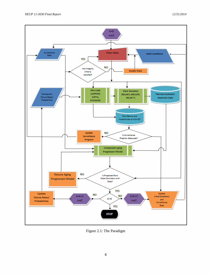
2. The Paradigm All nuclear power plants in the U.S. have at least a Level 1 PRA for assessing core damage frequency (CDF) and a limited Level 2 analysis that is focused on assessing the frequency of large early release (LERF). We refer to this type of PRA as a Level 1.5 PRA. The envisioned interaction of the degradation (or aging) models with the plant dynamics within a 1.5 PRA environment is schematically shown in Figure 2.1. The paradigm, in essence, augments the methodology of [4] for compatibility with the NGSC environment. At time t=0, plant state as obtained from the surveillance data, plant configuration and state of process variables (Initial Conditions) that constitute the Plant State are fed into the Plant Simulator. Plant State and Component Failure Rates/Probabilities are also fed into the PRA code for the prediction of Risk Metrics and Importances at t=T. The variable T is a user specified time interval, possibly chosen iteratively to represent the surveillance intervals or refueling outages, as well as degradation dynamics adequately. The Plant Simulator produces the thermal-hydraulic/neutronic data which are fed into the Component Aging Progression Models and assumed to stay constant within the time interval T to predict failure rates/probabilities at t=T. The Plant Simulator operates over two distinctly different time scales: 1) the quasi-steady state condition while the plant is at power during a fuel cycle, and, 2) the dynamic time frame of a reactor shutdown and startup or the transient response of the plant to an accident. For the quasi-steady state condition, it is likely that the thermal-hydraulic conditions will be maintained constant based on the results of off-line steady-state calculations performed with the Plant Simulator. Initial Conditions, Surveillance Data, maintenance and repair actions as they affect the Plant State are also updated at each time t=kT. If the observed Plant State is not consistent with the aging progression model predictions, Component Aging Progression Model is retuned. The time is incremented by T, failure rates/probabilities are updated and the process is repeated until the target time horizon KT is reached. At the end of each time interval kT, the plant state is re-evaluated as it impacts the determination of the Risk Metrics and Importances for that time interval. As degradation processes continue over the time period the potential will grow that an initiating event of some kind would occur, such as a leak or rupture of a pipe at a weld. Based on the condition, the likelihood of an initiating event of this nature will be determined, which will affect the plant risk for that time interval. Similarly, degradation will occur in components that need to operate in response to an initiating event, again affecting the outcome of the risk assessment. Thus, it is necessary not only to project degradation as a function of time but to interpret the impact of a level of degradation on the probability of the occurrence of an initiating event or the impact of
NEUP 11-3030 Final Report 12/31/2014
3
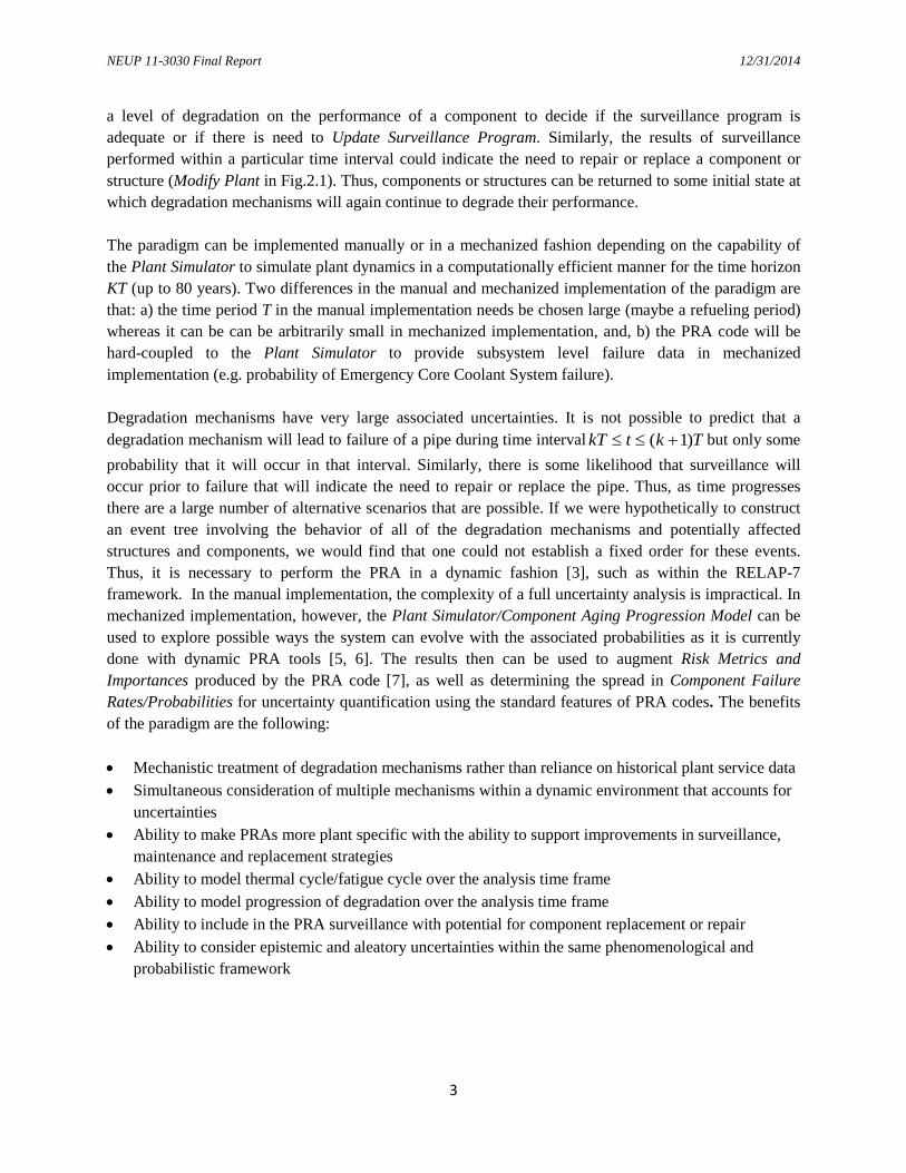
a level of degradation on the performance of a component to decide if the surveillance program is adequate or if there is need to Update Surveillance Program. Similarly, the results of surveillance performed within a particular time interval could indicate the need to repair or replace a component or structure (Modify Plant in Fig.2.1). Thus, components or structures can be returned to some initial state at which degradation mechanisms will again continue to degrade their performance. The paradigm can be implemented manually or in a mechanized fashion depending on the capability of the Plant Simulator to simulate plant dynamics in a computationally efficient manner for the time horizon KT (up to 80 years). Two differences in the manual and mechanized implementation of the paradigm are that: a) the time period T in the manual implementation needs be chosen large (maybe a refueling period) whereas it can be can be arbitrarily small in mechanized implementation, and, b) the PRA code will be hard-coupled to the Plant Simulator to provide subsystem level failure data in mechanized implementation (e.g. probability of Emergency Core Coolant System failure). Degradation mechanisms have very large associated uncertainties. It is not possible to predict that a degradation mechanism will lead to failure of a pipe during time interval ( 1)kT t k T≤ ≤ + but only some probability that it will occur in that interval. Similarly, there is some likelihood that surveillance will occur prior to failure that will indicate the need to repair or replace the pipe. Thus, as time progresses there are a large number of alternative scenarios that are possible. If we were hypothetically to construct an event tree involving the behavior of all of the degradation mechanisms and potentially affected structures and components, we would find that one could not establish a fixed order for these events. Thus, it is necessary to perform the PRA in a dynamic fashion [3], such as within the RELAP-7 framework. In the manual implementation, the complexity of a full uncertainty analysis is impractical. In mechanized implementation, however, the Plant Simulator/Component Aging Progression Model can be used to explore possible ways the system can evolve with the associated probabilities as it is currently done with dynamic PRA tools [5, 6]. The results then can be used to augment Risk Metrics and Importances produced by the PRA code [7], as well as determining the spread in Component Failure Rates/Probabilities for uncertainty quantification using the standard features of PRA codes. The benefits of the paradigm are the following: • Mechanistic treatment of degradation mechanisms rather than reliance on historical plant service data • Simultaneous consideration of multiple mechanisms within a dynamic environment that accounts for
uncertainties • Ability to make PRAs more plant specific with the ability to support improvements in surveillance,
maintenance and replacement strategies • Ability to model thermal cycle/fatigue cycle over the analysis time frame • Ability to model progression of degradation over the analysis time frame • Ability to include in the PRA surveillance with potential for component replacement or repair • Ability to consider epistemic and aleatory uncertainties within the same phenomenological and
probabilistic framework
NEUP 11-3030 Final Report 12/31/2014
4
Figure 2.1: The Paradigm

NEUP 11-3030 Final Report 12/31/2014
5
3. Passive Component Selection Reference [4] provides procedures for the selection of passive systems, structures and components (SSCs) to be considered for inclusion PRA. The first step is to develop an exhaustive catalog of the plant with regard to potential failure locations and the degradation mechanisms applicable to those portions of the plant. Although this involves a major activity on the part of the plant, it is one that has already been performed and reported in [8]. The analysts then identify for each of these areas those mechamisms with high susceptibility and high knowledge. References [4] and [8] mainly address degradation mechanisms applicable to the reactor coolant and power conversion systems. A study of containment degradation mechanisms performed by Sandia National Laboratories [9] provides at least a starting point for the identification of key degradation mechanisms for the containment structure of the plant being analyzed. The failure of a component must then be related back to the failure of SSCs in the scenarios analyzed in the plant PRA. For SSCs that extend over a long distance (e.g. piping), aging-vulnerable locations are identified from weld locations, pipe bends, areas of high residual stress, surveillance data, measured operating conditions or from the Plant Simulator. In order to limit the scope of the overall analysis, a preliminary risk screening would be performed. The typical approach taken for prioritizations of this type is the use of risk importance measures that involve modifying the reliability of a component, either to zero or one and observing the relative impact on plant risk. Measures of this type include risk reduction worth, risk achievement worth and Fussell-Vesely measure [4]. The risk increase measures are then ranked. Based on this ranking, a decision is then made regarding the passive SSCs to be included in PRA.
4. Physics Based Aging Degradation Models Under Consideration The following physics based aging models have been considered in this study:
• The state transition stress corrosion cracking (SCC) model of [10] • The parametric Scott model for SCC of steam generator (SG) tubes [11] • The KWU-KR model to describe flow accelerated corrosion (FAC) driven degradation [12]
These models are described in Sections 4.1, 4.2 and 4.3, respectively.
4.1 State Transition SCC Model This model has been developed for an Alloy 82/182 dissimilar metal weld in a pressurized water reactor (PWR) primary coolant system [10]. The component class is relevant to loss of coolant accident (LOCA) accident sequences in PWRs. Figure 4.1 shows the transition diagram for the model. State evolutions are described through

NEUP 11-3030 Final Report 12/31/2014
6
Figure 4.1: State Transition Model for Multi-State Degradation Process [10]
𝒅𝒅(𝒕)𝒅𝒕
= 𝑨(𝒕)𝒅(𝒕) (4. 1) where
𝒅(𝒕) =
⎣⎢⎢⎢⎢⎡
𝑆(𝑡)𝑀(𝑡)𝐶(𝑡)𝐷(𝑡)𝐿(𝑡)𝑅(𝑡) ⎦
⎥⎥⎥⎥⎤
and
𝑨(𝒕) =
⎣⎢⎢⎢⎢⎢⎡−𝜙1(𝑡) 𝜔1 𝜔3 𝜔2 𝜔4 0 𝜙1(𝑡) −(𝜔1 + 𝜙2(𝑡) + ∅3(𝑡)) 0 0 0 0
0 𝜙3(𝑡) −(𝜔3 + ∅6) 0 0 00 𝜙2(𝑡) 0 −(𝜙2 + 𝜙4(𝑡)) 0 00 0 0 𝜙4(𝑡) −(𝜔4 + 𝜙5) 00 0 𝜙6 0 𝜙5 0⎦
⎥⎥⎥⎥⎥⎤
(4.2)
with the components of X(t) defined as in Fig.4.1. The transition rates 𝜙5, 𝜙6 and ωi (i=1,2,3) are constant. Simplified version of the transition rates 𝜙𝑖(𝑡) for (i=1,…,4) in A(t ) as presented in [10] are
𝜙1(𝑡) = (𝑏/𝜏) �𝑡𝜏
�𝑏−1
(4.3)

NEUP 11-3030 Final Report 12/31/2014
7
𝜙2(𝑡) =
⎩⎪⎨
⎪⎧ 0 𝑖𝑖 𝑢 ≤
𝑎𝐷
�� 𝑀 𝑎𝐷𝑃𝐷/(𝑢 𝑎𝐷𝑃𝐷 + 𝑢2 �� 𝑀𝑃𝑐) 𝑖𝑖 𝑢 > 𝑎𝐷/�� 𝑀 𝑎𝑎𝑎 𝑢 ≤ 𝑎𝐶/�� 𝑀
𝑎𝐷𝑃𝐷
𝑢 𝑎𝐷𝑃𝐷 + 𝑢 𝑎𝐶 𝑃𝑐 𝑖𝑖 𝑢 >
𝑎𝐷
�� 𝑀 𝑎𝑎𝑎 𝑢 > 𝑎𝐶/�� 𝑀
(4.4)
𝜙3(𝑡) =
⎩⎪⎨
⎪⎧ 0 𝑖𝑖 𝑢 ≤ 𝑎𝐶
�� 𝑀
𝑎𝐶𝑃𝐶/(𝑢 𝑎𝐷𝑃𝐷 + 𝑢2 �� 𝑀𝑃𝑐) 𝑖𝑖 𝑢 > 𝑎𝐶/�� 𝑀 𝑎𝑎𝑎 𝑢 ≤ 𝑎𝐷/�� 𝑀 𝑎𝐶𝑃𝐶
𝑢 𝑎𝐷𝑃𝐷+𝑢 𝑎𝐶 𝑃𝑐 𝑖𝑖 𝑢 > 𝑎𝐶
�� 𝑀 𝑎𝑎𝑎 𝑢 > 𝑎𝐷/�� 𝑀
(4.5)
𝜙4(𝑡) = �1/𝑤 𝑖𝑖 𝑤 > (𝑎𝐿 − 𝑎𝐷)/�� 𝑀0 𝑜𝑡ℎ𝑒𝑒𝑤𝑖𝑒𝑒
(4.6)
The impact of thermal-hydraulic data on the transition rates is mainly through 𝜏 and 𝑎��. This impact is quantified through [13]
𝜏 = 𝐴𝜎𝑛𝑒(𝑄/𝑅𝑅) (4.7)
��𝑀 = 𝛼𝑖𝑎𝑎𝑎𝑎𝑎𝑖𝑎𝑜𝑖𝑜𝑛𝑜𝐾𝛽𝑒−��𝑄𝐺
𝑅 � (𝑅−1−𝑅𝑟𝑟𝑟−1)�
(4.8) In Eqs.(4.3) - (4.6), u is a time after crack initiation and w is time after macro-crack formation. The other parameters in Eqs.(4.2) - (4.8) are the following: b : Weibull shape parameter for crack initiation model τ : Weibull scale parameter for crack initiation model 𝑎𝐷 : Crack length threshold for radial macro-crack 𝑃𝐷: Probability that micro-crack evolves as radial crack 𝑃𝐶 : Probability that micro-crack evolves as circumferential crack 𝑎��: Maximum credible crack growth rate 𝑎𝐶 : Crack length threshold for circumferential macro-crack 𝑎𝐿 : Crack length threshold for leak ω1: Repair transition rate from micro-crack ω2 : Repair transition rate from radial macro-crack ω3 : Repair transition rate from circumferential macro-crack ω4: Repair transition rate from leak ∅5: Leak to rupture transition rate ∅6 : Macro-crack to rupture transition rate A: Fitting parameter that may include material and environmental dependences 𝜎: Explicit stress factor (MPa) n: Stress exponent factor Q : Crack initiation activation energy (kJ/mole) T: Operating temperature (ºK) R: Universal gas constant (8.314 x 10⁻³ kJ/mole-ºK) 𝛼: Fitting constant for crack growth amplitude – lognormal distribution
NEUP 11-3030 Final Report 12/31/2014
8
Tref : Reference temperature used to normalize data (°K)
𝑄𝐺: Thermal activation energy for crack growth (kJ/mole) K: Crack tip stress intensity factor (MPa√m) 𝑖𝑎𝑎𝑎𝑎𝑎 : 1.0 (for Alloy 182) 𝑖𝑎𝑜𝑖𝑜𝑛𝑜 : 1.0 (parallel to dendrite solidification direction) 𝛽: Stress intensity exponent (1.6) The repair rates refer to in-cycle inspection within the context of Fig.2.1. One of the challenging issues with the representation of the state transition diagram of Fig.4.1 through Eqs. (4.1)-(4.8) while maintaining consistency with the physics of the degradation process is the representation of the transition rates given in Eqs.(4.4)-(4.6). The reason is that while, for example, physically State D in Fig.4.1 will not be achieved before State M is achieved, State D will start being populated at time t=0 during the solution of Eqs.(4.1)-(4.8). On the other hand, 𝜙2(𝑡), 𝜙3(𝑡)and 𝜙4(𝑡)in Eqs.(4.4)-(4.6) depend on the residence times of the hardware under consideration in different states which cannot be accounted for directly through the formalism of Eqs.(4.1)-(4.8). For that reason, these equations were solved in [10] by partitioning the time interval of interest into 160 segments and augmenting the state space of Fig.4.1 by auxiliary variables which represent the probabilities of the States S, M, C, D, L and R being in each segment as a function of time. The resulting model has 6x160=960 states. While this approach is closer to physical reality, each of these 960 states will get populated starting from time t=0 during the solution of the resulting 960 differential equations as well. Thus, consistency with the physics of the process still remains a problem. Furthermore, the arbitrary discretization of the time horizon of interest brings a subjective element to the solution process and number of equations to be solved grows very rapidly with increasing number components to be modeled, as well as the temporal refinement of the solutions. A new approach to the problem was developed to meet these challenges through the use of the concept of sojourn times. The sojourn time, in essence, is the expected time that the system resides in a given state and is defined through
𝜏𝑛,𝑘 = � 𝑎𝑡 𝑡𝑝𝑛(𝑡) 𝑅𝑘
0 (4.9)
where 𝜏𝑛,𝑘 is the sojourn time in State n until time 𝑡 = 𝑇𝑘 and 𝑝𝑛(𝑡)𝑎𝑡 is the probability of being in State n within the time interval dt around t. The approach to the solution of the problem, while taking into account possible repair, was formulated as the following: Consider the semi-Markov process with sojourn time dependent transition rates
𝑎𝑥𝑛(𝑡)𝑎𝑡
= −𝑥𝑛(𝑡) � 𝜙𝑚𝑛(𝜏𝑛)𝑁
𝑚=1𝑚≠𝑛
+ � 𝜙𝑛𝑚(𝜏𝑚)𝑁
𝑚=1𝑚≠𝑛
𝑥𝑚(𝑡)(𝑎 = 1, ⋯ , 𝑁). (4.10)

NEUP 11-3030 Final Report 12/31/2014
9
where 𝜏𝑚 is the total sojourn time of the system in State m (𝑚 = 1, ⋯ , 𝑁), 𝑥𝑛(𝑡) is the probability that the system is in State n until time t, and 𝜙𝑚𝑛(𝜏𝑛) is the transition rate from State n to State m as a function of sojourn time. The solution involves the following steps:
1. Partition the time interval of into intervals of length Tk - Tk-1 =ΔTk-1 (k=1,…,K) with T0=0 2. For the interval ΔT0, solve Eq.(4.10) with 𝜏𝑚 = 0 (𝑚 = 1, ⋯ , 𝑁) 3. Let k=1 4. For the interval ΔTk let
𝜏𝑛,𝑘 = � 𝑎𝑡 (𝑡 − 𝑇𝑘−1)𝑎𝑥𝑛(𝑡)
𝑎𝑡
𝑅𝑘
𝑅𝑘−1 + 𝜏𝑛,𝑘−1. (4.11)
5. Calculate 𝜙𝑚𝑛𝑘 = 𝜙𝑚𝑛�𝜏𝑛,𝑘� ∀𝑎, 𝑚 = 1, ⋯ , 𝑁 and solve Eq.(4.10) with these transition rates and using 𝑥𝑛(𝑇𝑘−1 )(𝑎 = 1, ⋯ , 𝑁) as initial conditions. If repair has taken place for State n at the end of ΔTk, restore 𝜙𝑚𝑛�𝜏𝑛,𝑘� for all m=1,…,N to their initial values of 𝜙𝑚𝑛(0).
6. Let k=k+1 and go to Step 4.
In the algorithmic implementation of Step, Eq.(4.11) is converted into the differential equation to provide format consistency with Eqs.(4.10), as well as simplicity of implementation in the NGSC environment.
𝑎𝜏𝑛,𝑘(𝑡)𝑎𝑡 = (𝑡 − 𝑇𝑘−1) �−𝑥𝑛(𝑡) � 𝜙𝑚𝑛�𝜏𝑛,𝑘−1�
𝑁
𝑚=1𝑚≠𝑛
+ � 𝜙𝑛𝑚�𝜏𝑚,𝑘−1�𝑁
𝑚=1𝑚≠𝑛
𝑥𝑚(𝑡) � (4.12)
for (𝑇𝑘−1≤ t ≤𝑇𝑘; k=1,2,..K) For the comparison of this approach to the one used in [10], the semi-Markovian model was implemented for the data reported in [13] and also shown in Table 4.1 using MATLAB. The comparison is shown in Fig.4.2 below which indicates that the agreement is good. The differences can be partly explained in terms of the semi-discrete nature of the solution technique of [10] (i.e. transitions occur in 6 month intervals) versus the continuous time representation of the semi-Markov model. For example, the semi-Markov model predicts a lower leak probability because it accounts for repair continuously whereas [10] accounts for the repair in 6-month intervals. Similarly, while the probability of circumferential and radial crack state probabilities are of similar order for both [10] and the semi-Markov model, the differences between the two state probabilities are much closer to each other for t=80 years in the semi-Markov model results as expected since they both originate from the same micro-crack state with similar transition rates (see Fig.4.1). Also note that the initial state decreases more rapidly in the semi-Markov model because aging takes place on a continuous basis rather than in 6-month intervals as it does in [10].
Table 4.1: Model Parameters for the Comparison of Semi Markov Results to those reported in [10]
Model Input Parameter Value b- Weibull shape parameter for crack initiation model 2.0 τ - Weibull scale parameter for crack initiation model 4 years 𝑎𝐷 -Crack length threshold for radial macro-crack 10 mm 𝑃𝐷 - Probability that micro-crack evolves as radial crack 0.009

NEUP 11-3030 Final Report 12/31/2014
10
𝑎�� - Maximum credible crack growth rate 9.46 mm/yr 𝑎𝐶 - Crack length threshold for circumferential macro-crack 10 mm 𝑃𝐶 - Probability that micro-crack evolves as circumferential crack 0.001 𝑎𝐿 - Crack length threshold for leak 20 mm ω1- Repair transition rate from micro-crack 1 x10⁻³/yr ω2- Repair transition rate from radial macro-crack 2 x 10⁻²/yr ω3- Repair transition rate from circumferential macro-crack 2 x 10⁻²/yr ω4- Repair transition rate from leak 8 x10⁻¹ /yr ∅5- Leak to rupture transition rate 2 x 10⁻²/yr ∅6- Macro-crack to rupture transition rate 1 x 10⁻⁵/yr
[10] results Semi-Markov model results
Figure 4.2: Comparison of the semi-Markov model to the results reported in [10]
A graphical user interface (GUI) was developed in MATLAB for standalone implementations of the model, as well as interfacing with a quasi-steady state condition PRA while the plant is at power during a fuel cycle (agingGUI.m). A hardcopy of agingGUI.m and listing of the functions it calls is given in Appendix A. The GUI also provides capability for uncertainty quantification using Monte Carlo (MC) sampling. In the MC simulation of the multi-state physics based transition model, the history dependent transition rates given by Eqs,(4.3)-(4.6) are not sampled directly. Instead, the process holding time at State i (i.e., u or w) is sampled assuming uniform distribution within specified bounds and then the transition from State i to State j is determined. This procedure is repeated until the accumulated holding time reaches the predefined time horizon. The external influencing factors on crack initiation and crack growth such as pressure, temperature are taken from Plant Simulator in Fig.2.1 (e.g. RELAP-7) for each MC run.
The algorithm for the simulation of the process of component degradation on the time horizon [0,𝑡𝑚𝑎𝑚=60 years] is given by the following pseudo-code:
initialize the system is in state i = S (initial state: no flaw) set the time t = 0 (initial time) input the total number of replications Nmax set t* =0 set n=1

NEUP 11-3030 Final Report 12/31/2014
11
while n<Nmax while t< tmax,
take external influencing factors (T, P) data from RELAP-7 run sample a departure time t from the distribution function sample a random number ξ from the uniform distribution in [0, 1] for each outgoing transition (j = 0,1,… , M, j≠ i),
calculate the transition probability 𝜙𝑖𝑖(𝑡, 𝑇, 𝑃) If ∑ 𝜙𝑖𝑘(𝑡)𝑖−1
𝑘=0 <ξ < ∑ 𝜙𝑖𝑘(𝑡)𝑖𝑘=0
then activate the transition to state j end if
end for. set t*=t
remove the system from place i to place j end while set n=n+1
end while
Figure 4.3 shows an example input screen with corresponding results. In left hand side of the main window there are two frames: Model Parameters list controls for loading and managing input data for crack initiation and crack growth models and Latin hypercube sampling (LHS) parameters (number of realizations for epistemic and aleatory uncertainty) for two-loop uncertainty analysis (see Section 6.2). On left bottom there are Help and Result buttons. Help button serves for explaining the model and mechanism details and how the user can modify this model (for instance to build a 4-state semi-Markov model instead of a 6-state model to simulate stress corrosion cracking for a steam generator tube rupture scenario described in Section 6.3). Result button operates as a run command and calls all required functions to produce the sojourn time approach results (state probabilities vs time) and results of the two-loop uncertainty analysis on the right hand side of the window. The uncertainty analysis results are shown with mean value for leakage probability L(t) (red line) and rupture probability R(t) (blue line) as function of time, as well as the spread in L(t) and R(t) (gray bands around the mean values).
4.2 The Parametric Scott Model for SCC of SG Tubes [11]
The SG operates in a very demanding environment characterized by high pressure (~15 MPa) and temperatures (315-330℃) on the primary side. Because of these harsh conditions, steam generator degradation has been observed in industry almost immediately following the first PWR start-ups. Over the years, certain degradation mechanisms such as denting have become more manageable by special water chemistry controls, etc. However, SCC continues to be a significant problem in the industry today [14]. Figure 4.4 shows degradation mechanisms that have contributed to SG tube plugging as a function of time.

NEUP 11-3030 Final Report 12/31/2014
12
Figure 4.3: Main window of the GUI.
Figure 4.4: Degradation mechanisms responsible for SG tube plugging over the years
(adapted from [15]).
NEUP 11-3030 Final Report 12/31/2014
13
In that respect, SCC was considered as a primary degradation mechanism of the SG. SCC is of particular interest to plants operating with steam generators manufactured with mill-annealed (MA) Alloy 600. This material was found to be very susceptible to SCC, which drove efforts to form a new metal, Alloy 690, of choice for SG manufacturing. As of 2009, 10 (14%) plants in the United States had SGs with Alloy 600MA (mill annealed) tubes, 17 (25%) had SGs with Alloy 600TT (high temperature treated) tubes, and 42 (61%) had SGs with Alloy 690 tubes [14]. Alloy 690 is much more resistant to SCC but little industry operational data exist limiting ability to develop credible degradation models. As a result, our study models a plant that uses a Westinghouse-designed recirculating steam generator produced from Alloy 600MA tubes. This should be consistent with the basic event tree model being used (see Attachment), which is based on the NUREG-1150 Zion risk assessment [16]. One degradation rate model of interest for this study is described in [11] which is valid for longitudinal (axial) cracks of thin-walled elements
𝑎𝑎𝑎𝑡
= 2.8 ∙ 10−11 ∙ (𝐾 − 9)1.16 (4.13)
where 𝑎𝑎/𝑎𝑡 is crack growth rate (m/s) and K is the stress intensity factor (MPa∙√m). However, this model has been successfully applied outside of its initial assumptions in a study simulating surface crack growth [17]. In addition, Electric Power Research Institute (EPRI) developed a model based on Eq. (4.13) for thick-walled elements. On the other hand, since the ratio of thickness-to-diameter of steam tubes is less than 0.1, it is not clear that the EPRI model is applicable to the system under consideration.
4.3 The KWU-KR Model to describe FAC Driven Degradation [12] FAC of the carbon steel and the subsequent wall thinning is relevant for the secondary system components including the steam line. As the amount of material (steel) decreases, the capacity of the component to withstand the pressure drop across the pipe decreases. NUREG/CR-5632 [4] study emphasizes the importance of FAC on plant risk. It also provides a detailed review of available FAC models. One of these, the KWU-KR model [12] has been selected to describe the FAC-driven degradation of the steam line in our study because it is non-proprietary. Given the water/steam properties such as temperature and fluid chemistry to be obtained from the NGSC, the KWU-KR model can be used to calculate the decrease in effective wall thickness of a pipe with time. The thickness at which the pipe would rupture can then be determined by the load-capacity analysis. The load, here, is defined as the actual pressure differential experienced by the pipe. The capacity can be described as the pipe’s ability to withstand pressure, which is determined by pipe thickness, material composition, and temperature. The KWU-KR model determines the rate of wall thinning due to flow-accelerated corrosion. This approach accounts for Keller’s geometric factor, flow velocity, chemistry and temperature, piping metallurgy, and exposure time [4]. The model can be also adjusted to analyze two-phase flow. The specific rate of FAC is expressed as
𝛥𝜙𝑅,𝐾𝐾𝐾−𝐾𝑅 = 6.35𝑘𝑐(𝐵𝑒𝑁𝑁[1 − 0.175 ∙ (𝑝𝑝 − 7)2] ∙ 1.8𝑒−0.118𝑔 + 1) ∙ 𝑖(𝑡) (4.14)
𝐵 = −10.5√ℎ − 9.375 × 10⁻⁴ ∙ 𝑇2 + 0.79𝑇 − 132.5

NEUP 11-3030 Final Report 12/31/2014
14
𝑁 = �−0.0875ℎ − 1.275 × 10⁻⁵ ∙ 𝑇2 + 1.078 × 10⁻² ∙ 𝑇 − 2.15 (𝑖𝑜𝑒 0% ≤ ℎ ≤ 0.5%)
(−1.29 × 10⁻⁴ ∙ 𝑇2 + 0.109𝑇 − 22.07) ∙ 0.154 ∙ 𝑒1.2ℎ (𝑖𝑜𝑒 0.5% ≤ ℎ ≤ 5%)
where ΔϕR,KWU−KR: specific FAC rate (µg/(cm2h)) kc: Keller′s geometry factor w ∶ flow velocity (m/s) pH ∶ pH value g ∶ oxygen content (ppb) h ∶ content of chromium and molybdenum in steel (total %) T ∶ temperature (K) f(t): time correction factor In case of a two phase flow, the flow velocity, w, in Eq. (4.14) is modified as
𝑤𝐹 = 𝑚𝜌𝑊
1−𝑚𝑠𝑠1−𝛼
(4.15)
where
wF ∶ mean velocity in the water film on the inside surface (m/s) m ∶ mass flux (kg/(m2s)) ρw: density of the water at saturation condition (kg/m3 ) xst: steam quality α ∶ void fraction The time correction factor, f(t), in Eq. (4.14) is determined using Eq. (4.16) below. For short operating periods, the time factor approaches unity.
𝑖(𝑡) = 𝐶1 + 𝐶2𝑡 + 𝐶3𝑡2 + 𝐶4𝑡3 (4.16) where f(t): time correction factor t ∶ exposure time (hr) C1 = 9.999934 × 10⁻¹ C2 = −3.356901 × 10⁻⁷ C3 = −5.624812 × 10⁻¹¹ C4 = 3.849972 × 10⁻¹⁶
Specific pipe geometries and associated geometric factors, kc, in Eq. (4.14) are shown in Table 4.2.
Table 4.1: Keller’s Geometric factor, kc, in Eq. (4.14) (adapted from [4])
Pipe Geometry Keller’s Geometric Factor, kc

NEUP 11-3030 Final Report 12/31/2014
15
Straight tube 0.04 Leaky joints, labyrinths 0.08
Behind junctions 0.15 Behind tube inlet (sharp edge) 0.16
Elbow, R/D = 2.5 0.23 Elbow, R/D = 1.5 0.30 In and over blades 0.30 Elbow, R/D = 0.5 0.52
In branches #2 0.60 In branches #1 0.75
On tubes, on blade, or on plate 1.00
Equation (4.14) combined with information about the pipe’s material and exposure time is used to calculate wall corrosion, hc, as shown in Eq.(4.17).
ℎ𝐶(𝑡) = 𝛥𝜙𝑅𝑜𝜌𝑠𝑠
(4.17)
where hC(t) ∶ calculated thickness of pipe corroded away at time t (cm) ΔϕR ∶ specific FAC rate (µg/(cm2 h)) t ∶ exposure time (hr) ρst ∶ density of steel (µg/cm3) Given the original wall thickness and the corrosion rate, the wall thickness as a function of time is determined using Eq. (4.18)
ℎ𝑝𝑖𝑝𝑜(𝑡) = ℎ𝑎𝑜𝑖𝑔𝑖𝑛𝑎𝑎 − ℎ𝐶(𝑡) (4.18)
where
hpipe(t): pipe wall thickness at time t (cm) horiginal: nominal pipe wall thickness (cm) hC(t) ∶ calculated thickness of pipe corroded away at time t (cm)
5. Incorporation of Maintenance Activities into the Paradigm As indicated in Fig.2.1 Initial Conditions, Surveillance Data, maintenance and repair actions as they affect the Plant State are also updated at each time t=kT. If the observed Plant State is not consistent with the aging progression model predictions, Component Aging Progression Model is retuned. As also stated in Section 2, it is necessary not only to project degradation as a function of time but to interpret the impact of a level of degradation on the probability of the occurrence of an initiating event or the impact of a level of degradation on the performance of a component to decide if the surveillance program is adequate or if there is need to update the surveillance program. Finally, event sequences involving
NEUP 11-3030 Final Report 12/31/2014
16
repair/replacement actions need to be integrated into the PRA in a manner that does not lead to non-coherence. Appendix B provides an overview of methods that can be used for the surveillance and detection of crack precursors, as well as a Bayesian scheme that can be used to retune the aging model described in Section 4.1. Another approach, directed to the non-detection likelihood of cracks and which has been developed as part of M.S. thesis research performed within the scope of this project [18] is described in Section 5.1 using the SCC of SG tubes (Section 4.2) as an example case. A methodology for the incorporation of event sequences involving repair/replacement action is described in Section 5.2.
5.1 Probabilistic Treatment of Steam Generator Tube Failure As also described in the M.S. Thesis of R. Lewandowski [18] which evolved from the findings of this project, the probabilistic treatment begins by setting model parameters, including number of tubes, operating pressures, stresses, material properties, etc. Next, a simulation of crack growth in tubes is performed using one of the approaches described in Section 4. At the beginning of cycle i, cracks are introduced to a number of tubes according to an empirically-based lognormal distribution [19]. Within each ith cycle, the tubes are divided into 20 crack growth rate groups, using data from the Ringhals plant [20] to adjust the coefficient in Equation 4.13. At the end of cycle i, lengths of cracks initiated in previous cycles are updated. A group with cracks from the jth growth rate and introduced in the ith cycle is said to contain Ni,j tubes. The depth and length is the same for all Ni,j tubes. At the end of current cycle k, tubes are examined to see whether they need to be repaired (plugged). A crack first reaches depth requiring the tube to be plugged in cycle t (i.e. when k=t). Research performed by NRC on the effectiveness of eddy current testing indicates that at a crack depth at which the tube would be plugged or repaired (40% of the wall thickness) the probability of detection is only about 50%. However, as the crack depth approaches the wall thickness (a through-wall crack), the probability of detection is approximately98% [21]. One of the reasons that eddy current testing is not 100% reliable for a through-wall crack could be because of their proximity to structures in the SG. The cracks in the remaining 0.02·Ni,j, number of unplugged and potentially susceptible tubes continue to grow. The closest integer of this value is referred to as NUPS
i,j . In the subsequent cycle, it is assumed that the detection probability of a flawed but undetected tube belonging to NUPS
i,j is only 50% in view of no other information about the relationship of detection probability to crack growth and location. NUPS
i,j is taken as the sample size from which a distribution of the number of tubes that will be missed again is drawn. This binomial distribution, shown in Eq. (5.1), is used to calculate the probability of the number of tubes belonging to NUPS
i,j that will avoid detection in the cycle immediately following cycle t.
𝑃(𝑥|𝑁) = 𝑁!𝑚!(𝑁−𝑚)!
𝑝𝑚(1 − 𝑝)𝑁−𝑚 (5.1) where
N ∶ number of undetected tubes during the initial surveillance test, Ni,jUPS
p: non − detection probability x: number of undtected tubes at the end of the current cycle

NEUP 11-3030 Final Report 12/31/2014
17
Tubes from NUPS
i,j become susceptible to rupture r cycles after cycle t (i.e. when k=r). Given that the kth cycle of interest is equal to or greater than r, the probability of non-detection is equal to pk. Eq. (5.3) determines the probability of at least one tube failing from a set of tubes with cracks characterized by the jth growth rate and introduced during the ith cycle. In addition, it is possible to determine not only the probabilities for different number of tubes failing, but also the overall weighted tube failure probability, which is just the mean failure probability as shown in Eq. (5.4)
𝑃(𝑥|𝑁, 𝑘) =𝑁!
𝑥! (𝑁 − 𝑥)!𝑝𝑘𝑚(1 − 𝑝𝑘)𝑁−𝑚 (5.2)
𝑃(𝑥 ≥ 1|𝑁, 𝑘) = 1 − (1 − 𝑝𝑘)𝑁 (5.3)
𝐸(𝑥|𝑁, 𝑘) = � 𝑥𝑃(𝑥|𝑁, 𝑘) = 𝑁𝑝𝑘𝑁
𝑚=1
(5.4)
In Eqs .(5.2) - (5.4)
N: number of undetected tubes during the intial surveillance test, 𝑁𝑖,𝑖𝐾𝑃𝑈
p: non − detection probability x: number of undetected tubes k: cycle of interest During the kth cycle, it is possible that tubes with cracks introduced during different cycles are susceptible to rupture. In other words, cracks formed during cycles i, i+1, etc., may be susceptible during the cycle of interest if k>r. It is assumed that cracks introduced during different cycles and belonging to different growth rates are independent. For a given rate group j and cycle k containing tubes with cracks that have originated during different cycles, the probability of at least one tube failing is shown in Eq.(5.5). During the kth cycle, the probability of at least one tube failing across all crack growth rates and cycles of introduction is determined using Eq. (5.6). The expected number of tubes failing in cycle k is shown in Eq. (5.7).
𝑃�𝐴𝑖�𝑘� = 𝑃 �� 𝐴𝑖|𝑗, 𝑘𝑚
𝑖=1
� = 1 − �[1 − 𝑃(𝐴𝑖,𝑖|𝑘)]𝑚
𝑖=1
(5.5)
𝑃 �� 𝐴𝑖|𝑘20
𝑖=1
� = 1 − �[1 − 𝑃�𝐴𝑖|𝑘�]20
𝑖=1
(5.6)
𝐸(𝑥|𝑘) = 1 + � ��1 − 𝑁𝑖,𝑖𝑝𝑘�𝑚
𝑖=1
20
𝑖=1
(5.7)
In Eqs.(5.5)-(5.7), P(Aj│k) is the probability that x≥1 in group j given k and m is the number of cycles that introduced cracks in tubes that are now susceptible to rupture.

NEUP 11-3030 Final Report 12/31/2014
18
5.2 Modeling Repair/Replacement Action in the PRA As indicated in Section 2, two different time scales are under consideration for the PRA: 1) the quasi-steady state condition while the plant is at power during a fuel cycle, and, 2) the dynamic time frame of a reactor shutdown and startup or the transient response of the plant to an accident. In the case of quasi-steady state condition, the surveillance/maintenance is performed at the end of each time period kT (cycle) and input data for the PRA applicable to the next time period ( 1)kT t k T≤ ≤ + is updated by taking this surveillance/maintenance action into consideration. For the dynamic time frame or the case of the surveillance/maintenance during the cycle, repair/replacement action can lead to non-coherence in the traditional ET/FT approach and subsequent less conservative results if rare event approximation is used in the quantification. The state transition SCC model described in Section 4.1 avoids this situation by producing a probability of failure (or rate) for the relevant cycle and component through a semi-Markov model that accounts both for the aging and repair process during the cycle. In situations where the time dependent sequencing of surveillance/maintenance is relevant, the approach described in [22] and [23] for the PRA modeling of digital instrumentation and control systems can be used. Basically, the procedure involves: 1) appropriately placing the primary implicants obtained from the dynamic PRA tools [5, 6] in the existing PRA through the standard features of the PRA software such as SAPHIRE [24], CAFTA [25] and RISKMAN [26] using consistent naming convention for basic events, 2) using recovery rules (for SAPHIRE) to remove inconsistent event sequences, or to flag questionable sequences for post-processing, 3) generating the cut sets/prime implicants for the overall plant PRA, and, 5) exporting cut sets/prime implicants for post-processing with additional tools if necessary.
6. Example Implementations The example implementations consist of the following cases: 1. Impact of local conditions into the transition rates 2. Sensitivity of transition rates to uncertainties 3. Aging and maintenance impacts on a steam-line break (SLB), failure of a main steam isolation valve
(MSLIV) to close followed by steam generator tube rupture (SGTR) These cases are described in Sections 6.1, 6.2 and 6.3, respectively.
6.1 Impact of Local Conditions on Transition Rates Equations (4.4)-(4.8) show that SCC affected by local operating conditions and specifically by temperature. In order to investigate the impact of local temperature on SCC, temperature dependent data (see Table 6.1 below) for a 4-loop generic PWR pressurizer surge line pipe weld (Alloy 182) was generated by the simulation of a simplified model of a 3600 MWth 4-loop PWR under normal operating conditions with a 100 s run with RELAP Mod3.4 [27] as a surrogate to RELAP-7. The nodalization diagrams for the PWR are given in the Figure 6.1(a) and 6.2(b). Three loops are modeled together and the fourth loop is modeled separately. The pressurizer (see Fig.6.2 (b)) is represented by a time dependent volume with a pressure boundary (Node 158) and a pressure relief valve (Node 157). The cylindrical body of the pressurizer is modeled using a pipe (Node 150). A single junction (Node 151) connects the pressurizer to the pipe modeling the surge line (Node 152).
The temperature dependent model input parameters obtained from the simulation are shown in Table 6.1 for Segment 1 of Node 152 which represents the pressurizer surge line pipe in Fig.6.2(b) (marked with

NEUP 11-3030 Final Report 12/31/2014
19
red circle). All the other parameters in Eqs. (4.3)-(4.8) are as given in Table 4.1. In a plant specific application, the repair rates would be estimated using the procedures described in Section 5.
Table 6.1: Temperature dependent model input parameters for crack initiation and growth rate in Eqs.(4.3)-(4.8) for Alloy 182
Parameter Value T- operating temperature at crack location 610 K (400 K≤T≤650 K) 𝛽- stress intensity exponent 1.6 𝜎- explicit stress factor 106 MPa n- stress exponent factor -7 A- fitting parameter 2.524 ×10⁵ 𝛼- fitting constant for crack growth amplitude – lognormal distribution
1.5 x 10⁻¹²
Q-crack initiation activation energy 130 kJ/mol QG-thermal activation energy for crack growth 220 kJ/mol (220-230 kJ/mol) R- universal gas constant 8.314 x 10⁻³ kJ/mole-K 𝑖𝑎𝑎𝑎𝑎𝑎-crack growth rate factor to account for effect of alloy composition
1.0
𝑖𝑎𝑜𝑖𝑜𝑛𝑜- crack growth rate factor to account for crack orientation relative to the dendrite direction
1.0
(a)

NEUP 11-3030 Final Report 12/31/2014
20
(b)
Figure 6.1: RELAP 5 nodalization of the PWR: (a) plant, b) SG and pressurizer
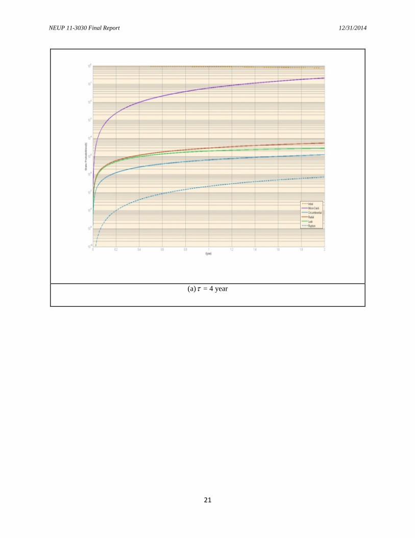
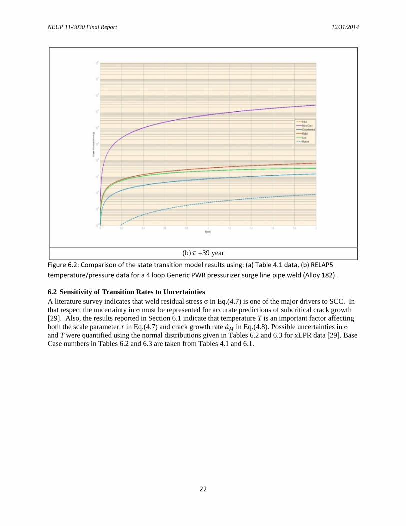
Figure 6.2 shows a comparison of results obtained earlier with using τ=4 yr versus a value of τ=150.6 yr obtained from Eqs.(4.3)-(4.8) with the data in Table 6.1. The rupture probability in Fig. 6.2(b) is lower than in Fig.6.2 (a) since the micro crack initiation rate obtained with Table 6.1 data is lower. Figure 6.2(a) assumes τ=4 years whereas τ determined from Table 6.1 data is 150.6 years, leading to a much smaller ϕ1(see Eq.(4.3)) and hence much slower micro crack initiation (see Fig.4.1). Also, using Table 6.1 data the crack growth rate Ma is calculated as 6.94 mm/yr instead of 9.46mm/yr assumed in Table 4.1. Therefore ϕ2, ϕ3 are staying zero for longer period (see Eqs.4.4 and 4.5, respectively) and hence initial transitions to both the circumferential and radial macro crack states are being delayed.
Figure 6.2 shows that the results, and in particular τ, are very sensitive to temperature. For example, a 40K increase in T would yield the value of τ=4 used in Table 4 to obtain Fig.6.2 (a) results. These results emphasize the need to use plant specific data dependent on local conditions rather than generic data in PRA.
NEUP 11-3030 Final Report 12/31/2014
21
(a)τ = 4 year
NEUP 11-3030 Final Report 12/31/2014
22
(b)τ =39 year
Figure 6.2: Comparison of the state transition model results using: (a) Table 4.1 data, (b) RELAP5 temperature/pressure data for a 4 loop Generic PWR pressurizer surge line pipe weld (Alloy 182).
6.2 Sensitivity of Transition Rates to Uncertainties A literature survey indicates that weld residual stress σ in Eq.(4.7) is one of the major drivers to SCC. In that respect the uncertainty in σ must be represented for accurate predictions of subcritical crack growth [29]. Also, the results reported in Section 6.1 indicate that temperature T is an important factor affecting both the scale parameter 𝜏 in Eq.(4.7) and crack growth rate ��𝑀 in Eq.(4.8). Possible uncertainties in σ and T were quantified using the normal distributions given in Tables 6.2 and 6.3 for xLPR data [29]. Base Case numbers in Tables 6.2 and 6.3 are taken from Tables 4.1 and 6.1.

NEUP 11-3030 Final Report 12/31/2014
23
Table 6.2: Definition of the inputs in Eq.(4.7) and their values used in different studies.
Crack Initiation Inputs Variable Description Unit Value
xLPR [29] Unwin[28] Base Case
T Operating temperature at crack location
K Distribution Type
Normal 617
610
Mean 617.9 Std. Deviation 0.0882 Deterministic 618
b Weibull shape parameter None 3 Distribution Type
Triangular 2 Minimum 3.915
Mode 4.35 Maximum 4.785
𝝈 Applied tensile stress factor MPa Distribution Type
Normal Distribution Type
Normal 106
Mean 300.3 Mean 300.3 Std. Deviation 110 Std.
Deviation 110
Deterministic 150 Deterministic 150 n Stress exponent factor None -4 Distribution
Type Triangular -7
Minimum -7.7 Mode -7 Maximum -6.3
A Fitting parameter None 0.04 2.524 ×10⁵
2.524 x 10⁵
𝑸𝑰 Crack initiation activation
energy kJ/mole 182.9 Distribution
Type Triangular 130
Minimum 116.73 Mode 129.7 Maximum 142.67
NEUP 11-3030 Final Report 12/31/2014
24
Table 6.3: Definition of the Inputs in Eq. (4.8) and Their Values used in Different Studies
Crack Growth Model Inputs Sym-bol
Description Unit Value xLPR [29] Unwin[30] Base Case
𝜷 Stress intensity exponent
None 1.6 Distribution Type
Triangular 1.6
Minimum 1.44 Mode 1.6 Maximum 1.76
𝜶 Fitting constant for crack growth amplitude
(m/s) (MPa-m0.5)1.6
9.82 x 10⁻¹³ Distribution Type
Normal 1.5 x 10⁻¹²
Threshold - Mean 8 x 10-13
Std. Deviation - 𝐐𝐆 Thermal
activation energy for crack growth
kJ/mole Distribution Type
Normal Distribution Type
Normal 130
Mean 130 Mean 130 Std. Deviation 5 Std. Deviation 5 Deterministic 130 Deterministic 130
𝒇𝒂𝒂𝒂𝒂𝒂 Common factor applied to all specimens fabricated from the same weld to account for weld heat processing and for weld fabrication
None Distribution Type
Lognormal 1.0 1.0
Mean 0.9989
Std. Deviation 1.835
Deterministic 1.075
𝒇𝒂𝒐𝒐𝒐𝒐𝒕 “within weld” factor accounts for specimens fabricated from the same weld
None 1.0 1.0 1.0
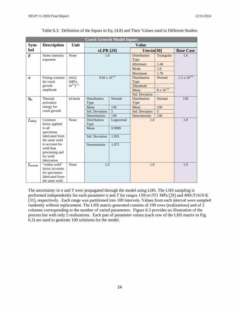
The uncertainty in σ and T were propagated through the model using LHS. The LHS sampling is performed independently for each parameter σ and T for ranges 150≤σ≤551 MPa [28] and 400≤T≤610 K [31], respectively. Each range was partitioned into 100 intervals. Values from each interval were sampled randomly without replacement. The LHS matrix generated consists of 100 rows (realizations) and of 2 columns corresponding to the number of varied parameters. Figure 6.3 provides an illustration of the process but with only 5 realizations. Each pair of parameter values (each row of the LHS matrix in Fig. 6.3) are used to generate 100 solutions for the model.

NEUP 11-3030 Final Report 12/31/2014
25
Figure 6.3: Schematic illustration of the uncertainty analysis performed with LHS for sampling size 5 and
for two parameters: temperature (T) and residual weld stress (σ) have normal distributions.
Figure 6.4 graphically represents the structure of Agingso_LHS.m which is a MATLAB code written to implement the LHS method. Listing of Agingso_LHS.m, as well as the other modules in Fig.6.4, are given in Appendix A.
Figure 6.4: Structure of Agingso_LHS
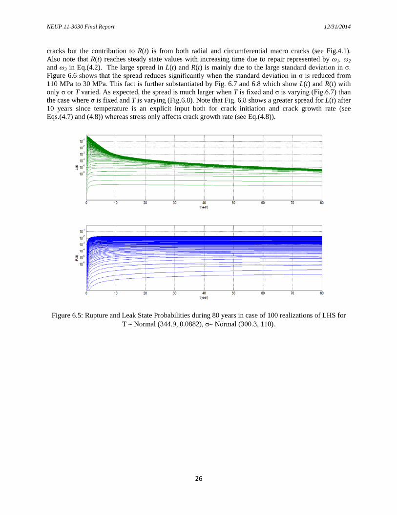
Figure 6.5 shows the results for the leak state probability L and rupture state probability of R as a function of time t over 80 years. The results show that there is initially a 4-5 order of magnitude spread in both L(t) and R(t) which becomes smaller for L(t) for large t since the contribution to L(t) is only from radial macro
NEUP 11-3030 Final Report 12/31/2014
26
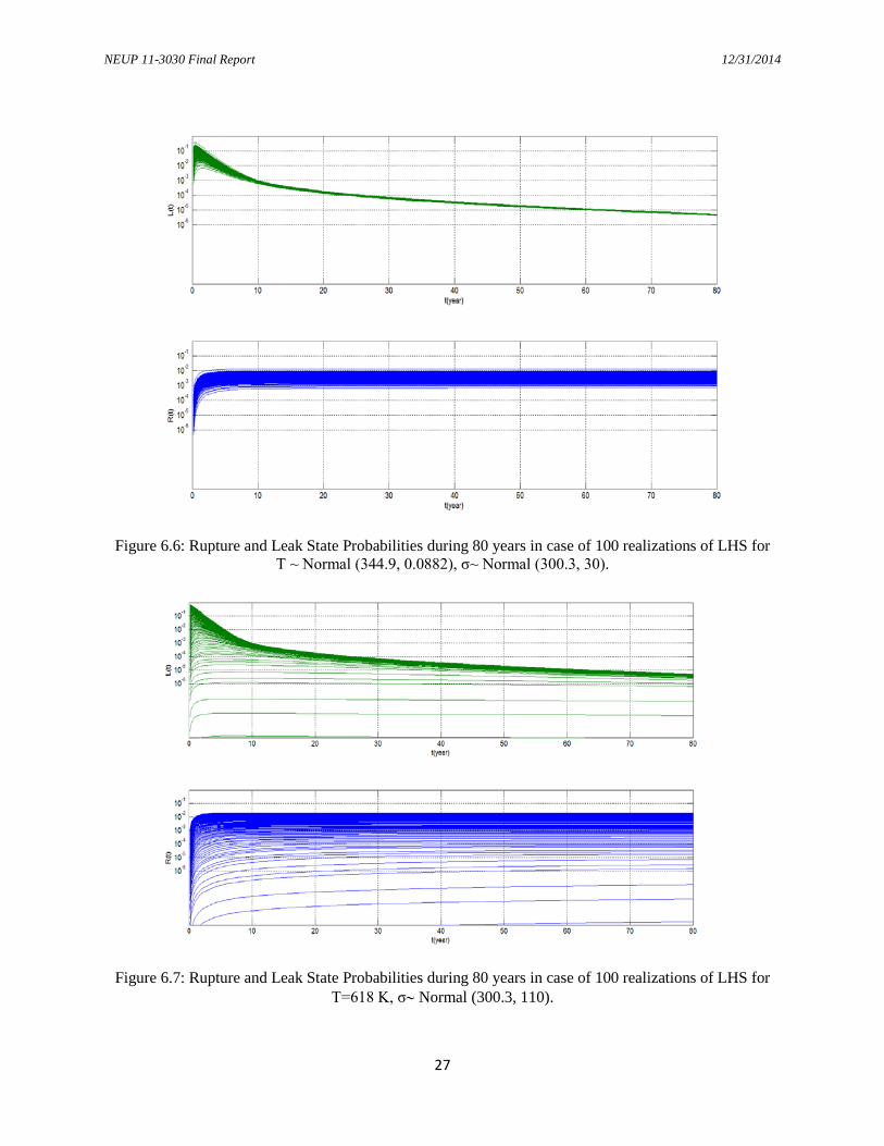
cracks but the contribution to R(t) is from both radial and circumferential macro cracks (see Fig.4.1). Also note that R(t) reaches steady state values with increasing time due to repair represented by ω1, ω2 and ω3 in Eq.(4.2). The large spread in L(t) and R(t) is mainly due to the large standard deviation in σ. Figure 6.6 shows that the spread reduces significantly when the standard deviation in σ is reduced from 110 MPa to 30 MPa. This fact is further substantiated by Fig. 6.7 and 6.8 which show L(t) and R(t) with only σ or T varied. As expected, the spread is much larger when T is fixed and σ is varying (Fig.6.7) than the case where σ is fixed and T is varying (Fig.6.8). Note that Fig. 6.8 shows a greater spread for L(t) after 10 years since temperature is an explicit input both for crack initiation and crack growth rate (see Eqs.(4.7) and (4.8)) whereas stress only affects crack growth rate (see Eq.(4.8)).
Figure 6.5: Rupture and Leak State Probabilities during 80 years in case of 100 realizations of LHS for
T ∼ Normal (344.9, 0.0882), σ∼ Normal (300.3, 110).
NEUP 11-3030 Final Report 12/31/2014
27
Figure 6.6: Rupture and Leak State Probabilities during 80 years in case of 100 realizations of LHS for
T ~ Normal (344.9, 0.0882), σ~ Normal (300.3, 30).
Figure 6.7: Rupture and Leak State Probabilities during 80 years in case of 100 realizations of LHS for
T=618 K, σ∼ Normal (300.3, 110).

NEUP 11-3030 Final Report 12/31/2014
28
Figure 6.8: Rupture and Leak State Probabilities during 80 years in case of 100 realizations of LHS for
T ∼ Normal (344.9, 30), σ=150 MPa.
Regarding the confidence levels on the distributions obtained for L(t) and R(t),as a function of time, the estimation was accomplished by computing the 95th and 5th percentiles of the distribution on the probability of leak L(t) and rupture R(t) at each time point. Figure 6.9 shows the distribution of the raw data (gray), as well as the 95th percentile (red) and 5th percentile (blue) confidence levels for L(t) and R(t) with T ~ Normal (617.9, 0.0882) [30] and σ ~ Normal (300.3, 110)[29]. The 95th percentile increases from 0 to a stable 0.01 around 10 years, which means that at least 5% of the results indicate 0.01 probability of rupture beyond 10 years. The magnitude and uncertainty on L(t) decreases with time as expected, since the leak is either repaired or leads to rupture.

NEUP 11-3030 Final Report 12/31/2014
29
Figure 6.9: Leak and Rupture State Probabilities during 80 years in case of 100 realizations of LHS for
T ∼ Normal (344.9, 0.0882), σ ∼ Normal (300.3, 110) Figures 6.10 and 6.11 examine trends in the relative importance of T vs. σ for rupture at various time points and indicate that there is a very complex relationship among stress, temperature and rupture probability R.

NEUP 11-3030 Final Report 12/31/2014
30
Figure 6.10: Rupture State Probabilities, stress and temperature realizations at t=10, 40 and 80 years in
case of 100 realizations of LHS for T ∼ Normal (617.9, 0.0882), σ∼ Normal (300.3, 110).
Figure 6.11: Rupture State Probabilities, stress and temperature realizations at t=40 and 60 years in case
of 100 realizations of LHS for T ∼ Normal (617.9, 0.0882), σ∼ Normal (300.3, 110).

NEUP 11-3030 Final Report 12/31/2014
31
Since it is very difficult to determine the trends from Figs.6.10 and 6.11, it was decided to develop a response surface from the data points. Figure 6.12 shows the impact of weld residual stress and temperature variations on the rupture probability at t=40 years in case of 100 realizations. In Fig. 6.12, the response surface clearly shows the consistency of the results and the greater sensitivity to the uncertainty in stress than to the uncertainty in temperature. The fitting was done by using the method of least squares and Eq. (6.1). Coefficients of Eq. (6.1) are listed in Table 6.4 and statistics goodness-of-fit data are summarized in Table 6.5.
20211
220011000),( σσσσ pTpTppTppTf +++++= (6.1)
Table 6.4: Fitting equation coefficients with 95% confidence bounds
Coefficients 95% confidence bounds
p00 = -24.39 -363.2, 314.5 p10 = -7.953 x10⁻⁵ -0.003004, 0.002845 p01 = 0.07899 -1.017, 1.175 p20 = 3.302 x10⁻⁷ 3.228 x10⁻⁷, 3.375 x10⁻⁷ p11 = -7.747 x10⁻⁸ -4.81 x10⁻⁶, 4.655 x10⁻⁶ p02 = -6.394 x10⁻⁵ -9.51 x10⁻⁵, 8.231 x10⁻⁴
Table 6.5: Statistic goodness-of-fit data
Goodness of fit SSE: 2.457 x10⁻⁷ R-square: 0.9995
Adjusted R-square: 0.9995 RMSE: 5.113 x10⁻⁵

NEUP 11-3030 Final Report 12/31/2014
32
Three Dimensional Response Surface of Rupture Probability
Projection of the Response Surface
Figure 6.12: Rupture probability change as a function of temperature (T) and weld stress (σ) at 40 years.
An issue that has been often brought up in uncertainty analyses is whether there is need to distinguish between epistemic and aleatory uncertainties. Whether in theory there is a fundamental separable difference between these two types of uncertainty has been hotly debated. To the decision-maker, however, there is a difference in how the results are displayed and interpreted depending on how they are classified.
When both aleatory and epistemic uncertainties are present in the model, it has been suggested by some that adequate treatment of both types of uncertainties would require a two-step simulation. As illustrated in the xLPR report [29] one way to do that is to have the inner loop and outer loop address the aleatory uncertainties and the epistemic uncertainties, respectively. In the outer loop, parameter values are sampled from epistemic uncertainty distributions and passed on to the inner loop. For each sample in the outer loop, LHS draws from aleatory uncertainty distributions are performed in the inner loop over the

NEUP 11-3030 Final Report 12/31/2014
33
time-frame of interest accounting for the aleatory uncertainty. From these results an average rupture probability can be calculated. From the outer loop analysis, it is therefore possible to obtain a distribution of the average rupture probabilities. This distribution provides measures of the uncertainty in rupture probability that could be reduced by further experimentation or model development. As LHS is also used to generate epistemic uncertainty, the simple arithmetic mean of the rupture probability over epistemic uncertainty yields the expected value <R> of the rupture probability. i.e.,
⟨𝑅⟩ = 1
𝑁∑ � 1
𝑀∑ 𝑅𝑚𝑛
𝑀𝑚=1 �𝑁
𝑛=1 (6.1) where M is the number of aleatory draws, N is the number of epistemic draws and 𝑅𝑚𝑛 are the rupture probabilities calculated from the state transition model for each draw combination. In general, it is expected that the overall average value will be the same regardless of whether the sampling is performed in a single-step or a two-step process. However, to test whether the overall average is affected by the sampling approach, a comparison was made of the two-step LHS versus single step LHS. Uncertainty in T and σ were characterized using normal PDFs: T ∼ Normal (617.9, 0.0882), σ∼ Normal (300.3, 30)) for both cases. In the two-step LHS, the uncertainty for T and σ were characterized as epistemic and aleatory, respectively, instead of both as epistemic. Equation (6.2) was implemented with N=100 and M=100 resulting in a total of 10,000 realizations. The single-step LHS realization was also performed for 10,000 draws to obtain ⟨𝑅⟩. Figure 6.12 shows the comparison of single step and two-step LHS sampling processes and Fig. 6.13 shows ⟨𝑅⟩ as a function of time for the single-step and two-step LHS. The temperature draws TN in Fig. 1 are for every 2 years. As can be seen in Fig. 6.13, difference between two methods is extremely small (on the order of 10-5) as expected.
a. Single Step LHS b. Two-Step LHS
Figure 6.13: Illustration of single step and two-step LHS comparisons.

NEUP 11-3030 Final Report 12/31/2014
34
Figure 6.14: Comparison of single-step and two-step LHS results.
6.3 Aging and Maintenance Impacts on a SLB/MSLIV/SGTR Scenario The case study analyzed in this research involves an accident scenario, in which steam generator tubes degraded by SCC due to depressurization following a SGTR from FAC. The study uses the process described in Section 3 for scenario selection using the data available in NUREG-1150 [16] and NUREG/CR-4550 Vol. 7 [32], the models presented in Sections 4.2 and 4.3 to account for SCC and FAC, respectively, and the approach presented in Section 5.1 to account for maintenance/repair. The response of a typical PWR to a hypothetical accident scenario is represented with an event-tree. The study incorporates all the quasi-static paradigm steps in shown in Fig.2.1 and has led to the M.S. Thesis of Radoslaw Lewandowski [18] which is included as an attachment to this report. The application of the model to the Zion Nuclear Power Station has indicated that the maximum core damage frequency over the plant lifetime for a steam line break-induced tube rupture would occur in the 20th year of plant operation. The model also predicts the time progression of tube plugging and the frequency of spontaneous steam generator tube ruptures. Based on historical data, the rates of degradation calculated in the analysis appear to be reasonable, but somewhat conservative.
7. Conclusion and Recommendations for Future Work This study has formulated a paradigm for the inclusion of passive component failure in an existing PRA both: a) in a quasi-static manner using the traditional ET/FT approach, and, b) in a dynamic fashion when the sequencing of events is conditioned on the physical conditions predicted in a simulation environment, such as the NGSC concept. The paradigm has been implemented for Alloy 82/182 dissimilar metal weld in a PWR primary coolant system to illustrate accounting for passive component failures in the dynamic implementation of the PRA and for a SLB/MSLIV/SGTR scenario under SCC and FAC in a PWR to illustrate its use in a quasi-static manner. The findings of the study show the need for using physics based

NEUP 11-3030 Final Report 12/31/2014
35
models capable of accounting for local conditions for realistically modeling aging degradation in PRAs and that the paradigm is implementable to accomplish this purpose in a computationally feasible fashion. The study has also led to six conference proceedings [33-38] and one M.S. thesis [18]. One journal paper submitted to Nuclear Engineering and Design is under review process1. The study is also expected to lead to one Ph.D. dissertation (Askin Guler) and at least two additional journal papers. This study used RELAP5/MOD3 as a surrogate for RELAP-7 to illustrate how aging degradation can be accounted for in a dynamic PRA environment. Future work needs to incorporate the algorithm described in Section 4.1 and illustrated in Section 6.1 into the RAVEN [39]/RELAP-7 environment under development at the Idaho National Laboratory (INL). One of the participants of this project, Askin Guler, visited INL as an intern during Summer 2014 to initiate the work which is currently being continued by the INL staff.
1 R. Lewandowski, R. Denning, T. Aldemir, J. Zhang, “Development of a Living, Condition-Dependent Probabilistic Safety Assessment”

NEUP 11-3030 Final Report 12/31/2014
36
8. References 1. S. M. HESS, N. DINH, J. P. GAERTNER, R, SZILARD, “Risk-Informed Safety Margin
Characterization”, ICONE 17, American Society of Mechanical Engineers (2009). 2. R. NOURGALIEV, N. DINH, R. YOUNGBLOOD, Development, Selection, Implementation, and
Testing of Architectural Features and Solution Techniques for Next Generation of System Simulation Codes to Support the Safety Case of the LWR Life Extension, INL/EXT-10-19984, Idaho National Laboratory Idaho Falls, ID (2010).
3. T. ALDEMIR, M. BELHADJ, L. DINCA, “Process Reliability and Safety Under Uncertainties”, Reliab. Engng & System Safety, 52, 211-225 (June 1996).
4. C. L. SMITH, V. N. SHAH, T. KAO, G. APOSTOLAKIS, “Incorporating Aging Effects into Probabilistic Risk Assessment — A Feasibility Study Utilizing Reliability Physics Models, NUREG/CR-5632, U.S. Nuclear Regulatory Commission, Washington, D.C. (2001).
5. A. HAKOBYAN, T. ALDEMIR, R. DENNING, S. DUNAGAN, D. KUNSMAN, B. RUTT, and U. CATALYUREK, “Dynamic generation of accident progression event trees," Nuclear Engineering and Design, 238, 3457-3467 (2008).
6. K. METZROTH, R. WINNINGHAM, U. CATALYUREK, R. DENNING, and T. ALDEMIR, "Linking of the RELAP5-3D Thermal-Hydraulic Code with the ADAPT PRA Tool," Trans.Am.Nucl.Soc., 100, 448-449 (2009).
7. T. ALDEMIR, M. P. STOVSKY, J. KIRSCHENBAUM, D. MANDELLI, P. BUCCI, L. A. MANGAN, D. W. MILLER, X. SUN, E. EKICI, S. GUARRO, M. YAU, B. W. JOHNSON, C. ELKS, and S. A. ARNDT, “Dynamic Reliability Modeling of Digital Instrumentation and Control Systems for Nuclear Reactor Probabilistic Risk Assessments”, NUREG/CR-6942, U.S. Nuclear Regulatory Commission, Washington, D.C. (2007).
8. P.L. ANDERSEN et al, Expert Panel Report on Proactive Materials Degradation Assessment, NUREG/CR-6923, U.S. Nuclear Regulatory Commission, Washington, D.C. (2007).
9. J. L. CHERRY, J.A. SMITH, Capacity of Steel and Concrete Containment Vessels with Corrosion Damage, NUREG/CR-6706, U.S. Nuclear Regulatory Commission, Washington, D.C. (2007).
10. S. D. UNWIN, P.P. LOWRY, R.F. LAYTON Jr., P. G. HEASLER, AND M. B. TOLOCZKO “Multi-State Physics Models of Aging Passive Components In Probabilistic Risk Assessment”, ANS PSA 2011 International Topical Meeting on Probabilistic Safety Assessment and Analysis, Wilmington, NC, March 13-17, 2011, on CD-ROM, American Nuclear Society, LaGrange Park, IL (2011).
11. P. M. SCOTT, “An Analysis of Primary Water Stress Corrosion Cracking in PWR Steam Generators”, Proc. of the Specialists Meeting on Operating Experience with Steam Generators, 16-22, Nuclear Energy Agency, Paris, France (1991).
12. W. KASTNER, E. RIEDLE, “Empirical Model for Calculation of Material Losses Due to Corrosion Erosion,” VGB Kraftwerkstechnik, 66, 1023-1029 (1986).
13. S.D. UNWIN, K.I. JOHNSON, R.F. LAYTON, P.P. LOWRY, S.E.SCOTT AND M.B. TOLOCZKO, “Physics-Based Stress Corrosion Cracking Component Reliability Model cast in an R7-Compatible Cumulative Damage Framework”, PNNL-20596, Pacific Northwest National Laboratory, (2011).
14. U.S. NUCLEAR REGULATORY COMMISSION, Backgrounder on Steam Generator Tube Issues (Available from: http://www.nrc.gov/reading-rm/doc-collections/fact-sheets/steam-gen.html)
15. D. R. DIERCKS, W.J. SHACK, J. MUSCARA, “Overview of Steam Generator Tube Degradation and Integrity Issues”, Nuclear Engineering and Design, 194, 19-30 (1999).

NEUP 11-3030 Final Report 12/31/2014
37
16. U.S. NUCLEAR REGULATORY COMMISSION, Severe Accident Risks: An Assessment for Five U.S. Nuclear Power Plants, NUREG-1150, U.S. Nuclear Regulatory Commission, Washington, D.C. (1990).
17. K. I. SHIN et al, “Simulation of stress corrosion crack growth in steam generator tubes”, Nuclear Engineering and Design, 214, 91-101 (2002).
18. R. LEWANDOWSKI, Incorporation of Corrosion Mechanisms into a State-dependent Probabilistic Risk Assessment, M.S. Thesis, The Ohio State University, Columbus, Ohio (2013).
19. Staehle, R.W., “Historical Review on Stress Corrosion Cracking of Ni-based Alloys – The Coriou Effect”. (Presented at CEA, January 26, 2010. To be published).
20. Wu, G., A probabilistic-mechanistic approach to modeling stress corrosion cracking propagation in Alloy 600 components with applications, in Mechanical Engineering 2011, University of Maryland: College Park.
21. D. S. Kupperman et al., “Eddy Current Reliability Results from the Steam Generator Mock-up Analysis Round-Robin”, NUREG/CR-6791, October 2009.
22. T. ALDEMIR, S. GUARRO, J. KIRSCHENBAUM, D. MANDELLI, L. A. MANGAN, P. BUCCI, M. YAU,,B. JOHNSON, C. ELKS, E. EKICI, M. P. STOVSKY, D. W. MILLER, X. SUN, S. A. ARNDT, Q. NGUYEN, J. DION, “A Benchmark Implementation of Two Dynamic Methodologies for the Reliability Modeling of Digital Instrumentation and Control Systems”, NUREG/CR-6985, U.S. Nuclear Regulatory Commission, Washington, D.C. (February 2009).
23. T. ALDEMIR, M.P. STOVSKY, J. KIRSCHENBAUM, D. MANDELLI, P. BUCCI, L.A. MANGAN, D.W. MILLER, X. SUN, E. EKICI, S. GUARRO, M. YAU, B. JOHNSON, C. ELKS, AND, S. A. ARNDT, “Dynamic Reliability Modeling of Digital Instrumentation and Control Systems for Nuclear Reactor Probabilistic Risk Assessments”, NUREG/CR-6942, U. S. Nuclear Regulatory Commission, Washington, D.C. (August 2007).
24. C. L. SMITH, J. KNUDSEN, M. CALLEY, S. BECK, K. KVARFORDT and S. T. WOOD, SAPHIRE Basics: An Introduction to Probability Risk Assessment Via the Systems Analysis Program for Hands-on Integrated Reliability Evaluations (SAPHIRE) Software, Idaho National Laboratory, Idaho Falls, ID (2005).
25. CAFTA For Windows, Version 3.0c, SAIC, Los Altos, California (1995). 26. RISKMAN 7.1 for Windows, ABS Consulting, Irvine, California (2003). 27. C. D. FLETCHER, R.R. SCHULTZ, RELAP5/MOD3 User Guidelines, NUREG/CR-5535, U. S.
Nuclear Regulatory Commission, Washington, D.C. (1992). 28. K. METZROTH, “A Comparison of Dynamic and Classical Event Tree Analysis for Nuclear Power
Plant Probabilistic Safety/Risk Assessment”, Ph.D. Dissertation, The Ohio State University (2011). 29. U.S. NUCLEAR REGULATORY COMMISSION, Models and Inputs Developed for Use in the
xLPR Pilot Study, Electric Power Research Institute, (1994). 30. S. D. UNWIN, K. I. JOHNSON, P. W.ESLINGER, Robustness of RISMC Insights under
Alternative Aleatory/Epistemic Uncertainty Classifications Draft Report, PNNL-21810, Pacific Northwest National Laboratory, Richland, WA (September 2012).
31. ELECTRIC POWER RESEARCH INSTITUTE, Materials Reliability Program Crack Growth Rates for Evaluating Primary Water Stress Corrosion Cracking of Alloy 82,182, and 132 Welds, EPRI Report MRP-115, 1006696, Palo Alto, CA (2003).

NEUP 11-3030 Final Report 12/31/2014
38
32. M. B. SATTISON, K.W. HALL, “Analysis of core damage frequency from internal events: Zion Unit 1. NUREG/CR-4550 Office of Nuclear Regulatory Research. U.S. Nuclear Regulatory Commission, Washington, D.C. (1989).
33. A. GULER, T. ALDEMIR, R. DENNING, “The Sojourn Time Approach for Modeling Aging in Passive Components”, Trans. Am. Nucl. Soc., 108, 552-554 (June 2013).
34. A. GULER, T. ALDEMIR, R. DENNING, “Multi-State Physics Based Aging Assessment of PWR Steam Generator Tube Rapture in Case of Primary Water Stress Corrosion Cracking”, Trans. Am. Nucl. Soc., 111, 104-106 (November 2014).
35. A. GULER, D. MANDELLI, A. ALFONSI, J. COGLIATI, C. RABITI, T. ALDEMIR, “Methodology for the Incorporation of Passive Component Aging Modeling into the RAVEN/ RELAP-7 Environment”, Trans. Am. Nucl. Soc., 111,920-923 (November 2014).
36. A. GULER, T. ALDEMIR, R. DENNING, “Multi-State Physics Based Aging Assessment of Passive Components”, Proc. ANS PSA 2013 International Topical Meeting on Probabilistic Safety Assessment and Analysis, CD-ROM, American Nuclear Society, LaGrange Park, IL (September 2013).
37. A. GULER, T. ALDEMIR, R. DENNING, “Uncertainty Evaluation in Multi-State Physics Based Aging Assessment of Passive Components”, Proc. PSAM 12, Paper #379, International Association for Probabilistic Safety Assessment and Management, California (June 2014).
38. R. LEWANDOWSKI, R. DENNING, T. ALDEMIR, AND J. ZHANG, “Development of a Dynamic, Plant Condition-Dependent Probabilistic Safety Assessment”, Proc. PSAM 12, Paper #279, International Association for Probabilistic Safety Assessment and Management, California (June 2014).
39. C. RABITI, A. ALFONSI, J. COGLIATI, D. MANDELLI and R. KINOSHITA “Reactor Analysis and Virtual Control Environment (RAVEN)”, INL/EXT-12-27351, Idaho national Laboratory, Idaho Falls, ID (2012).

NEUP 11-3030 Final Report 12/31/2014
39
APPENDIX A: The MATLAB Graphical User Interface Aging_GUI.m and Related Functions function varargout = untitled(varargin) gui_Singleton = 1; gui_State = struct('gui_Name', mfilename, ... 'gui_Singleton', gui_Singleton, ... 'gui_OpeningFcn', @untitled_OpeningFcn, ... 'gui_OutputFcn', @untitled_OutputFcn, ... 'gui_LayoutFcn', [] , ... 'gui_Callback', []); if nargin && ischar(varargin{1}) gui_State.gui_Callback = str2func(varargin{1}); end if nargout [varargout{1:nargout}] = gui_mainfcn(gui_State, varargin{:}); else gui_mainfcn(gui_State, varargin{:}); end % End initialization code - DO NOT EDIT % --- Executes just before untitled is made visible. function untitled_OpeningFcn(hObject, eventdata, handles, varargin) % This function has no output args, see OutputFcn. % hObject handle to figure % eventdata reserved - to be defined in a future version of MATLAB % handles structure with handles and user data (see GUIDATA) % varargin command line arguments to untitled (see VARARGIN) % Choose default command line output for untitled handles.output = hObject; sojournTimeApproach (handles); lhs5(handles); lhs4(handles); % Update handles structure guidata(hObject, handles); % UIWAIT makes untitled wait for user response (see UIRESUME) % uiwait(handles.figure1); % --- Outputs from this function are returned to the command line. function varargout = untitled_OutputFcn(hObject, eventdata, handles) % varargout cell array for returning output args (see VARARGOUT); % hObject handle to figure % eventdata reserved - to be defined in a future version of MATLAB % handles structure with handles and user data (see GUIDATA)

NEUP 11-3030 Final Report 12/31/2014
40
% Get default command line output from handles structure varargout{1} = handles.output; % --- Executes on button press in pushbutton1. function pushbutton1_Callback(hObject, eventdata, handles) % hObject handle to pushbutton1 (see GCBO) % eventdata reserved - to be defined in a future version of MATLAB % handles structure with handles and user data (see GUIDATA) sojournTimeApproach(handles); lhs5(handles); lhs4(handles); function lhs4(handles) cla(handles.axes4) cla(handles.axes4,'reset') axes(handles.axes4) % Sample size N runm=str2double(get(handles.edit5,'String')); runn=str2double(get(handles.edit6,'String')); %------------user defined model parameters------------------------------- bo=str2double(get(handles.edit2,'String')) ;%weibull shape parameter to=str2double(get(handles.edit3,'String')) ; %weibull scale parameter ad=str2double(get(handles.edit7,'String'));%crack lenght treshold for radial crack ac=str2double(get(handles.edit8,'String'));%crack lenght treshold for circumferential crack al=str2double(get(handles.edit9,'String')); % crack lenght threshold for leakage Pd=str2double(get(handles.edit10,'String')); %radial crack probability per year Pc=str2double(get(handles.edit11,'String')); %circumferantial crack probability per year w1=str2double(get(handles.edit12,'String')); %repair transition rate from micro-crack per yr w2=str2double(get(handles.edit13,'String')); %repair transition rate from radial macro-crack per yr w3=str2double(get(handles.edit14,'String')); %repair transition rate from circum. macro-crack per yr

NEUP 11-3030 Final Report 12/31/2014
41
w4=str2double(get(handles.edit15,'String')); %repair transition rate from leak per yr q5=str2double(get(handles.edit16,'String')); %leak to rupture transition rate per yr q6=str2double(get(handles.edit17,'String')); %macro-crack to rupture transition rate per yr %aleatory part% % %% LHS MATRIX % Parameter_settings_LHS; T_LHS=LHS_Call(600, 617.9, 650, 0.0882 ,runm,'norm'); sigma_LHS=LHS_Call(150,300.3,551,30,runn,'norm'); %% LHS MATRIX and PARAMETER LABELS LHSmatrix=[T_LHS]; LHSmattrix=[sigma_LHS]; t0=1e-30; tf=80; x0=[1 0 0 0 0 0 0 0 0]'; t1=0;t2=0;t3=0; b=x0'; for z=1:runn z t0=1e-30; tf=80; x0=[1 0 0 0 0 0 0 0 0]'; t1=0;t2=0;t3=0; b=x0'; for y=1:runm %Run solution x times choosing different values f=@ODE_LHS; LHSmatrix(y); LHSmattrix(z); t1=0;t2=0;t3=0; m1=[]; t0=1e-30; tf=80; x0=[1 0 0 0 0 0 0 0 0]'; t1=0;t2=0;t3=0; b=x0'; for tf=1e-20:0.1:2 [t,x]=ode15s(@(t,x)f(t,x,LHSmatrix,LHSmattrix,y,z,runm,runn,t1,t2,t3,bo,to,ad,ac,al,Pd,Pc,w1,w2,w3,w4,q5,q6),[t0 tf],x0,[]); xTemp= x(end,1:9); m1 = [m1;xTemp]; x0 = xTemp'; t1=abs(x0(7,1)); t2=abs(x0(8,1));

NEUP 11-3030 Final Report 12/31/2014
42
t3=abs(x0(9,1)); t0 = tf; end m=[]; m=[m;b]; t0=1.99; for tf=2:2:80 [t,x]=ode15s(@(t,x)f(t,x,LHSmatrix,LHSmattrix,y,z,runn,runm,t1,t2,t3,bo,to,ad,ac,al,Pd,Pc,w1,w2,w3,w4,q5,q6),[t0 tf],x0,[]); xTemp= x(end,1:9); m = [m;xTemp]; x0 = xTemp'; t1=abs(x0(7,1)); t2=abs(x0(8,1)); t3=abs(x0(9,1)); t0 = tf; end p=m; L1_lhs(:,y)=m1(:,5); R1_lhs(:,y)=m1(:,6); L_lhs(:,y)=p(:,5); R_lhs(:,y)=p(:,6); end R_ep(:,z)=sum(R_lhs,2)/runm; R_ep1(:,z)=sum(R1_lhs,2)/runm; %% i=(0:2:80);whos semilogy(handles.axes4,i,p(:,6),'color', [0.8 0.8 0.8]), xlabel('t(year)'), ylabel('R(t)'); axis(handles.axes4,[0 tf 1.0E-10 1]); grid on set(gca,'YTick',[10^-6,10^-5,10^-4,10^-3,10^-2,10^-1]) hold on semilogy(handles.axes4,1e-20:0.1:2,m1(1:21,6),'color', [0.8 0.8 0.8]); axis([0 tf 1.0E-10 1]); grid on set(gca,'YTick',[10^-6,10^-5,10^-4,10^-3,10^-2,10^-1]) end R_f=sum(R_ep,2)/runn; R_f1=sum(R_ep1,2)/runn; i=(0:2:80);whos

NEUP 11-3030 Final Report 12/31/2014
43
semilogy(handles.axes4,i,p(:,6),'b'), xlabel('t(year)'), ylabel('R(t)'); hold on function lhs5(handles) cla(handles.axes5) cla(handles.axes5,'reset') axes(handles.axes5) % Sample size N runm=str2double(get(handles.edit5,'String')); runn=str2double(get(handles.edit6,'String')); %------------user defined model parameters------------------------------- bo=str2double(get(handles.edit2,'String')) ;%weibull shape parameter to=str2double(get(handles.edit3,'String')) ; %weibull scale parameter ad=str2double(get(handles.edit7,'String'));%crack lenght treshold for radial crack ac=str2double(get(handles.edit8,'String'));%crack lenght treshold for circumferential crack al=str2double(get(handles.edit9,'String')); % crack lenght threshold for leakage Pd=str2double(get(handles.edit10,'String')); %radial crack probability per year Pc=str2double(get(handles.edit11,'String')); %circumferantial crack probability per year w1=str2double(get(handles.edit12,'String')); %repair transition rate from micro-crack per yr w2=str2double(get(handles.edit13,'String')); %repair transition rate from radial macro-crack per yr w3=str2double(get(handles.edit14,'String')); %repair transition rate from circum. macro-crack per yr w4=str2double(get(handles.edit15,'String')); %repair transition rate from leak per yr q5=str2double(get(handles.edit16,'String')); %leak to rupture transition rate per yr q6=str2double(get(handles.edit17,'String')); %macro-crack to rupture transition rate per yr %aleatory part% % %% LHS MATRIX % Parameter_settings_LHS; T_LHS=LHS_Call(600, 617.9, 650, 0.0882 ,runm,'norm');
NEUP 11-3030 Final Report 12/31/2014
44
sigma_LHS=LHS_Call(150,300.3,551,30,runn,'norm'); %% LHS MATRIX and PARAMETER LABELS LHSmatrix=[T_LHS]; LHSmattrix=[sigma_LHS]; t0=1e-30; tf=80; x0=[1 0 0 0 0 0 0 0 0]'; t1=0;t2=0;t3=0; b=x0'; for z=1:runn z t0=1e-30; tf=80; x0=[1 0 0 0 0 0 0 0 0]'; t1=0;t2=0;t3=0; b=x0'; for y=1:runm %Run solution x times choosing different values f=@ODE_LHS; LHSmatrix(y); LHSmattrix(z); t1=0;t2=0;t3=0; m1=[]; %m1=[m1;b]; t0=1e-30; tf=80; x0=[1 0 0 0 0 0 0 0 0]'; t1=0;t2=0;t3=0; b=x0'; for tf=1e-20:0.1:2 [t,x]=ode15s(@(t,x)f(t,x,LHSmatrix,LHSmattrix,y,z,runm,runn,t1,t2,t3 ,bo,to,ad,ac,al,Pd,Pc,w1,w2,w3,w4,q5,q6 ),[t0 tf],x0,[]); xTemp= x(end,1:9); m1 = [m1;xTemp]; x0 = xTemp'; t1=abs(x0(7,1)); t2=abs(x0(8,1)); t3=abs(x0(9,1)); t0 = tf; end m=[]; m=[m;b]; t0=1.99; for tf=2:2:80 % time(tf)=tf; [t,x]=ode15s(@(t,x)f(t,x,LHSmatrix,LHSmattrix,y,z,runn,runm,t1,t2,t3,bo,to,ad,ac,al,Pd,Pc,w1,w2,w3,w4,q5,q6),[t0 tf],x0,[]); %[rows,cols]=size(x); xTemp= x(end,1:9);

NEUP 11-3030 Final Report 12/31/2014
45
m = [m;xTemp]; x0 = xTemp'; t1=abs(x0(7,1)); t2=abs(x0(8,1)); t3=abs(x0(9,1)); t0 = tf; end p=m; L1_lhs(:,y)=m1(:,5); R1_lhs(:,y)=m1(:,6); L_lhs(:,y)=p(:,5); R_lhs(:,y)=p(:,6); end R_ep(:,z)=sum(R_lhs,2)/runm; R_ep1(:,z)=sum(R1_lhs,2)/runm; %% i=(0:2:80);whos semilogy(handles.axes5,i,p(:,5),'color', [0.8, 0.8, 0.8]), xlabel('t(year)'), ylabel('L(t)'); axis([0 tf 1.0E-10 1]); grid on set(gca,'YTick',[10^-6,10^-5,10^-4,10^-3,10^-2,10^-1]) hold on semilogy(handles.axes5,1e-20:0.1:2,m1(1:21,5),'color',[0.8,0.8,0.8]); axis([0 tf 1.0E-10 1]); hold on end R_f=sum(R_ep,2)/runn; R_f1=sum(R_ep1,2)/runn; %% Save the workspace save Model_LHS.mat; %% i=(0:2:80);whos semilogy(handles.axes5,i,p(:,5),'r'), xlabel('t(year)'), ylabel('L(t)'); hold on title('\fontsize{16}LHS Results'); hold on function sojournTimeApproach( handles)

NEUP 11-3030 Final Report 12/31/2014
46
cla(handles.axes6) cla(handles.axes6,'reset') axes(handles.axes6); format long t0=1e-15; tp=0; x0=[1 tp tp tp tp tp tp tp tp]'; b=x0'; %------------user defined model parameters------------------------------- bo=str2double(get(handles.edit2,'String')) ;%weibull shape parameter to=str2double(get(handles.edit3,'String')) ; %weibull scale parameter ad=str2double(get(handles.edit7,'String'));%crack lenght treshold for radial crack ac=str2double(get(handles.edit8,'String'));%crack lenght treshold for circumferential crack al=str2double(get(handles.edit9,'String')); % crack lenght threshold for leakage Pd=str2double(get(handles.edit10,'String')); %radial crack probability per year Pc=str2double(get(handles.edit11,'String')); %circumferantial crack probability per year w1=str2double(get(handles.edit12,'String')); %repair transition rate from micro-crack per yr w2=str2double(get(handles.edit13,'String')); %repair transition rate from radial macro-crack per yr w3=str2double(get(handles.edit14,'String')); %repair transition rate from circum. macro-crack per yr w4=str2double(get(handles.edit15,'String')); %repair transition rate from leak per yr q5=str2double(get(handles.edit16,'String')); %leak to rupture transition rate per yr q6=str2double(get(handles.edit17,'String')); %macro-crack to rupture transition rate per yr %-------------sojourn time approach---------------------------------------- t1=0;t2=0;t3=0; m1=[]; m1=[m1;b]; for tf=1e-20:0.1:2 % time(tf)=tf; [t,x]=ode45(@agingso,[t0 tf],x0,[],t1,t2,t3,bo,to,ad,ac,al,Pd,Pc,w1,w2,w3,w4,q5,q6); %[rows,cols]=size(x); xTemp= x(end,1:9); m1 = [m1;xTemp];
NEUP 11-3030 Final Report 12/31/2014
47
x0 = xTemp'; t1=abs(x0(7,1)); t2=abs(x0(8,1)); t3=abs(x0(9,1)); t0 = tf; end m=[]; m=[m;b]; t0=1.99 for tf=2:2:80 [t,x]=ode45(@agingso,[t0 tf],x0,[],t1,t2,t3,bo,to,ad,ac,al,Pd,Pc,w1,w2,w3,w4,q5,q6); xTemp= x(end,1:9); m = [m;xTemp]; x0 = xTemp'; t1=abs(x0(7,1)); t2=abs(x0(8,1)); t3=abs(x0(9,1)); t0 = tf; end p=m; i=(0:2:80);whos semilogy(handles.axes6,i,p(:,3),'b',i,p(:,4),'r',i,p(:,5),'g',i,p(:,6),'--b'), xlabel('t(year)'), ylabel('State Probabilities(t)'); hold on semilogy(handles.axes6,i,p(:,2),'color',[0.5 0 0.5]); hold on semilogy(handles.axes6, i,p(:,1),'color',[1 .5 0]); hold on semilogy(handles.axes6, 1e-20:0.1:2,m1(1:21,3),'b',1e-20:0.1:2,m1(1:21,4),'r',1e-20:0.1:2,m1(1:21,5),'g',1e-20:0.1:2,m1(1:21,6),'--b'), xlabel('t(year)'), ylabel('State Probabilities(t)'); hold on semilogy(handles.axes6,1e-20:0.1:2,m1(1:21,2),'color',[0.5 0 0.5]); legend( 'Circumferential','Radial','Leak','Rupture','Micro-Crack','Initial','Location','southeast') axis(handles.axes6,[0 tf 1.0E-10 1]); grid on set(gca,'YTick',[10^-6,10^-5,10^-4,10^-3,10^-2,10^-1]) title(['\fontsize{16}Sojourn Approach Results']) hold all function edit2_Callback(hObject, eventdata, handles)

NEUP 11-3030 Final Report 12/31/2014
48
% hObject handle to edit2 (see GCBO) % eventdata reserved - to be defined in a future version of MATLAB % handles structure with handles and user data (see GUIDATA) % Hints: get(hObject,'String') returns contents of edit2 as text % str2double(get(hObject,'String')) returns contents of edit2 as a double % --- Executes during object creation, after setting all properties. function edit2_CreateFcn(hObject, eventdata, handles) % hObject handle to edit2 (see GCBO) % eventdata reserved - to be defined in a future version of MATLAB % handles empty - handles not created until after all CreateFcns called % Hint: edit controls usually have a white background on Windows. % See ISPC and COMPUTER. if ispc && isequal(get(hObject,'BackgroundColor'), get(0,'defaultUicontrolBackgroundColor')) set(hObject,'BackgroundColor','white'); end function edit3_Callback(hObject, eventdata, handles) % hObject handle to edit3 (see GCBO) % eventdata reserved - to be defined in a future version of MATLAB % handles structure with handles and user data (see GUIDATA) % Hints: get(hObject,'String') returns contents of edit3 as text % str2double(get(hObject,'String')) returns contents of edit3 as a double % --- Executes during object creation, after setting all properties. function edit3_CreateFcn(hObject, eventdata, handles) % hObject handle to edit3 (see GCBO) % eventdata reserved - to be defined in a future version of MATLAB % handles empty - handles not created until after all CreateFcns called % Hint: edit controls usually have a white background on Windows. % See ISPC and COMPUTER. if ispc && isequal(get(hObject,'BackgroundColor'), get(0,'defaultUicontrolBackgroundColor')) set(hObject,'BackgroundColor','white'); end function edit4_Callback(hObject, eventdata, handles)

NEUP 11-3030 Final Report 12/31/2014
49
% hObject handle to edit4 (see GCBO) % eventdata reserved - to be defined in a future version of MATLAB % handles structure with handles and user data (see GUIDATA) % Hints: get(hObject,'String') returns contents of edit4 as text % str2double(get(hObject,'String')) returns contents of edit4 as a double % --- Executes during object creation, after setting all properties. function edit4_CreateFcn(hObject, eventdata, handles) % hObject handle to edit4 (see GCBO) % eventdata reserved - to be defined in a future version of MATLAB % handles empty - handles not created until after all CreateFcns called % Hint: edit controls usually have a white background on Windows. % See ISPC and COMPUTER. if ispc && isequal(get(hObject,'BackgroundColor'), get(0,'defaultUicontrolBackgroundColor')) set(hObject,'BackgroundColor','white'); end function edit5_Callback(hObject, eventdata, handles) % hObject handle to edit5 (see GCBO) % eventdata reserved - to be defined in a future version of MATLAB % handles structure with handles and user data (see GUIDATA) % Hints: get(hObject,'String') returns contents of edit5 as text % str2double(get(hObject,'String')) returns contents of edit5 as a double % --- Executes during object creation, after setting all properties. function edit5_CreateFcn(hObject, eventdata, handles) % hObject handle to edit5 (see GCBO) % eventdata reserved - to be defined in a future version of MATLAB % handles empty - handles not created until after all CreateFcns called % Hint: edit controls usually have a white background on Windows. % See ISPC and COMPUTER. if ispc && isequal(get(hObject,'BackgroundColor'), get(0,'defaultUicontrolBackgroundColor')) set(hObject,'BackgroundColor','white'); end function edit6_Callback(hObject, eventdata, handles)

NEUP 11-3030 Final Report 12/31/2014
50
% hObject handle to edit6 (see GCBO) % eventdata reserved - to be defined in a future version of MATLAB % handles structure with handles and user data (see GUIDATA) % Hints: get(hObject,'String') returns contents of edit6 as text % str2double(get(hObject,'String')) returns contents of edit6 as a double % --- Executes during object creation, after setting all properties. function edit6_CreateFcn(hObject, eventdata, handles) % hObject handle to edit6 (see GCBO) % eventdata reserved - to be defined in a future version of MATLAB % handles empty - handles not created until after all CreateFcns called % Hint: edit controls usually have a white background on Windows. % See ISPC and COMPUTER. if ispc && isequal(get(hObject,'BackgroundColor'), get(0,'defaultUicontrolBackgroundColor')) set(hObject,'BackgroundColor','white'); end % --- Executes on button press in pushbutton2. function pushbutton2_Callback(hObject, eventdata, handles) % hObject handle to pushbutton2 (see GCBO) % eventdata reserved - to be defined in a future version of MATLAB % handles structure with handles and user data (see GUIDATA) h = msgbox('This semi-Markov aging model simulates stress corrosion cracking mechanism. 6 states exist: Initial, micro-crack, circumferential macro-crack, radial macro-crack, leakage and rupture. This model can be applied to all SCC and Markov model states can be modified.','Help'); function edit7_Callback(hObject, eventdata, handles) % hObject handle to edit7 (see GCBO) % eventdata reserved - to be defined in a future version of MATLAB % handles structure with handles and user data (see GUIDATA) % Hints: get(hObject,'String') returns contents of edit7 as text % str2double(get(hObject,'String')) returns contents of edit7 as a double % --- Executes during object creation, after setting all properties. function edit7_CreateFcn(hObject, eventdata, handles) % hObject handle to edit7 (see GCBO) % eventdata reserved - to be defined in a future version of MATLAB

NEUP 11-3030 Final Report 12/31/2014
51
% handles empty - handles not created until after all CreateFcns called % Hint: edit controls usually have a white background on Windows. % See ISPC and COMPUTER. if ispc && isequal(get(hObject,'BackgroundColor'), get(0,'defaultUicontrolBackgroundColor')) set(hObject,'BackgroundColor','white'); end function edit8_Callback(hObject, eventdata, handles) % hObject handle to edit8 (see GCBO) % eventdata reserved - to be defined in a future version of MATLAB % handles structure with handles and user data (see GUIDATA) % Hints: get(hObject,'String') returns contents of edit8 as text % str2double(get(hObject,'String')) returns contents of edit8 as a double % --- Executes during object creation, after setting all properties. function edit8_CreateFcn(hObject, eventdata, handles) % hObject handle to edit8 (see GCBO) % eventdata reserved - to be defined in a future version of MATLAB % handles empty - handles not created until after all CreateFcns called % Hint: edit controls usually have a white background on Windows. % See ISPC and COMPUTER. if ispc && isequal(get(hObject,'BackgroundColor'), get(0,'defaultUicontrolBackgroundColor')) set(hObject,'BackgroundColor','white'); end function edit9_Callback(hObject, eventdata, handles) % hObject handle to edit9 (see GCBO) % eventdata reserved - to be defined in a future version of MATLAB % handles structure with handles and user data (see GUIDATA) % Hints: get(hObject,'String') returns contents of edit9 as text % str2double(get(hObject,'String')) returns contents of edit9 as a double % --- Executes during object creation, after setting all properties. function edit9_CreateFcn(hObject, eventdata, handles) % hObject handle to edit9 (see GCBO) % eventdata reserved - to be defined in a future version of MATLAB

NEUP 11-3030 Final Report 12/31/2014
52
% handles empty - handles not created until after all CreateFcns called % Hint: edit controls usually have a white background on Windows. % See ISPC and COMPUTER. if ispc && isequal(get(hObject,'BackgroundColor'), get(0,'defaultUicontrolBackgroundColor')) set(hObject,'BackgroundColor','white'); end function edit10_Callback(hObject, eventdata, handles) % hObject handle to edit10 (see GCBO) % eventdata reserved - to be defined in a future version of MATLAB % handles structure with handles and user data (see GUIDATA) % Hints: get(hObject,'String') returns contents of edit10 as text % str2double(get(hObject,'String')) returns contents of edit10 as a double % --- Executes during object creation, after setting all properties. function edit10_CreateFcn(hObject, eventdata, handles) % hObject handle to edit10 (see GCBO) % eventdata reserved - to be defined in a future version of MATLAB % handles empty - handles not created until after all CreateFcns called % Hint: edit controls usually have a white background on Windows. % See ISPC and COMPUTER. if ispc && isequal(get(hObject,'BackgroundColor'), get(0,'defaultUicontrolBackgroundColor')) set(hObject,'BackgroundColor','white'); end function edit11_Callback(hObject, eventdata, handles) % hObject handle to edit11 (see GCBO) % eventdata reserved - to be defined in a future version of MATLAB % handles structure with handles and user data (see GUIDATA) % Hints: get(hObject,'String') returns contents of edit11 as text % str2double(get(hObject,'String')) returns contents of edit11 as a double % --- Executes during object creation, after setting all properties. function edit11_CreateFcn(hObject, eventdata, handles) % hObject handle to edit11 (see GCBO) % eventdata reserved - to be defined in a future version of MATLAB

NEUP 11-3030 Final Report 12/31/2014
53
% handles empty - handles not created until after all CreateFcns called % Hint: edit controls usually have a white background on Windows. % See ISPC and COMPUTER. if ispc && isequal(get(hObject,'BackgroundColor'), get(0,'defaultUicontrolBackgroundColor')) set(hObject,'BackgroundColor','white'); end function edit12_Callback(hObject, eventdata, handles) % hObject handle to edit12 (see GCBO) % eventdata reserved - to be defined in a future version of MATLAB % handles structure with handles and user data (see GUIDATA) % Hints: get(hObject,'String') returns contents of edit12 as text % str2double(get(hObject,'String')) returns contents of edit12 as a double % --- Executes during object creation, after setting all properties. function edit12_CreateFcn(hObject, eventdata, handles) % hObject handle to edit12 (see GCBO) % eventdata reserved - to be defined in a future version of MATLAB % handles empty - handles not created until after all CreateFcns called % Hint: edit controls usually have a white background on Windows. % See ISPC and COMPUTER. if ispc && isequal(get(hObject,'BackgroundColor'), get(0,'defaultUicontrolBackgroundColor')) set(hObject,'BackgroundColor','white'); end function edit13_Callback(hObject, eventdata, handles) % hObject handle to edit13 (see GCBO) % eventdata reserved - to be defined in a future version of MATLAB % handles structure with handles and user data (see GUIDATA) % Hints: get(hObject,'String') returns contents of edit13 as text % str2double(get(hObject,'String')) returns contents of edit13 as a double % --- Executes during object creation, after setting all properties. function edit13_CreateFcn(hObject, eventdata, handles) % hObject handle to edit13 (see GCBO) % eventdata reserved - to be defined in a future version of MATLAB
NEUP 11-3030 Final Report 12/31/2014
54
% handles empty - handles not created until after all CreateFcns called % Hint: edit controls usually have a white background on Windows. % See ISPC and COMPUTER. if ispc && isequal(get(hObject,'BackgroundColor'), get(0,'defaultUicontrolBackgroundColor')) set(hObject,'BackgroundColor','white'); end function edit14_Callback(hObject, eventdata, handles) % hObject handle to edit14 (see GCBO) % eventdata reserved - to be defined in a future version of MATLAB % handles structure with handles and user data (see GUIDATA) % Hints: get(hObject,'String') returns contents of edit14 as text % str2double(get(hObject,'String')) returns contents of edit14 as a double % --- Executes during object creation, after setting all properties. function edit14_CreateFcn(hObject, eventdata, handles) % hObject handle to edit14 (see GCBO) % eventdata reserved - to be defined in a future version of MATLAB % handles empty - handles not created until after all CreateFcns called % Hint: edit controls usually have a white background on Windows. % See ISPC and COMPUTER. if ispc && isequal(get(hObject,'BackgroundColor'), get(0,'defaultUicontrolBackgroundColor')) set(hObject,'BackgroundColor','white'); end function edit15_Callback(hObject, eventdata, handles) % hObject handle to edit15 (see GCBO) % eventdata reserved - to be defined in a future version of MATLAB % handles structure with handles and user data (see GUIDATA) % Hints: get(hObject,'String') returns contents of edit15 as text % str2double(get(hObject,'String')) returns contents of edit15 as a double % --- Executes during object creation, after setting all properties. function edit15_CreateFcn(hObject, eventdata, handles) % hObject handle to edit15 (see GCBO) % eventdata reserved - to be defined in a future version of MATLAB

NEUP 11-3030 Final Report 12/31/2014
55
% handles empty - handles not created until after all CreateFcns called % Hint: edit controls usually have a white background on Windows. % See ISPC and COMPUTER. if ispc && isequal(get(hObject,'BackgroundColor'), get(0,'defaultUicontrolBackgroundColor')) set(hObject,'BackgroundColor','white'); end function edit16_Callback(hObject, eventdata, handles) % hObject handle to edit16 (see GCBO) % eventdata reserved - to be defined in a future version of MATLAB % handles structure with handles and user data (see GUIDATA) % Hints: get(hObject,'String') returns contents of edit16 as text % str2double(get(hObject,'String')) returns contents of edit16 as a double % --- Executes during object creation, after setting all properties. function edit16_CreateFcn(hObject, eventdata, handles) % hObject handle to edit16 (see GCBO) % eventdata reserved - to be defined in a future version of MATLAB % handles empty - handles not created until after all CreateFcns called % Hint: edit controls usually have a white background on Windows. % See ISPC and COMPUTER. if ispc && isequal(get(hObject,'BackgroundColor'), get(0,'defaultUicontrolBackgroundColor')) set(hObject,'BackgroundColor','white'); end function edit17_Callback(hObject, eventdata, handles) % hObject handle to edit17 (see GCBO) % eventdata reserved - to be defined in a future version of MATLAB % handles structure with handles and user data (see GUIDATA) % Hints: get(hObject,'String') returns contents of edit17 as text % str2double(get(hObject,'String')) returns contents of edit17 as a double % --- Executes during object creation, after setting all properties. function edit17_CreateFcn(hObject, eventdata, handles) % hObject handle to edit17 (see GCBO) % eventdata reserved - to be defined in a future version of MATLAB

NEUP 11-3030 Final Report 12/31/2014
56
% handles empty - handles not created until after all CreateFcns called % Hint: edit controls usually have a white background on Windows. % See ISPC and COMPUTER. if ispc && isequal(get(hObject,'BackgroundColor'), get(0,'defaultUicontrolBackgroundColor')) set(hObject,'BackgroundColor','white'); end function xdot=agingso(t,x,t1,t2,t3,bo,to,ad,ac,al,Pd,Pc,w1,w2,w3,w4,q5,q6) xdot=zeros(9,1); %% Constant Model Parameters adotmx=9.46; %max. credible crack growth rate %% Time Dependent Transition Rates (piecewise functions) q1=@(t1) (bo/to).*(t1/to)^(bo-1); %t is time from last repair q2=@(t2) (t2<=ad/adotmx).*0+(t2>ad/adotmx & t2>ac/adotmx).*(ad*Pd/(t2*ad*Pd+t2^2*adotmx*Pc)); %(t>ad/adotmx & t<=ac/adotmx).*(ad*Pr/(t*ad*Pr+t^2*adotmx*Pc)) q3=@(t2) (t2<=ac/adotmx).*0+(t2>ad/adotmx & t2>ac/adotmx).*(ac*Pc/(t2*ad*Pd+t2^2*adotmx*Pc)); q4=@(t3) (t3>((al-ad)/adotmx)).*(1/t3)+(t3<=((al-ad)/adotmx)).*0; %% Differential Equations xdot(1)=-q1(t).*x(1)+w1.*x(2)+w3.*x(3)+w2.*x(4)+w4.*x(5); xdot(2)=q1(t).*x(1)-(w1+q2(t)+q3(t)).*x(2); xdot(3)=q3(t).*x(2)-(w3+q6).*x(3); xdot(4)=q2(t).*x(2)-(w2+q4(t)).*x(4); xdot(5)=q4(t).*x(4)-(w4+q5).*x(5); xdot(6)=q6.*x(3)+q5.*x(5); %-------------sojourn time approach---------------------------------------- xdot(7)=abs(t.*xdot(1)); % Initial State sojourn time xdot(8)=abs(t.*xdot(2)); % Micro-Crack State sojourn time xdot(9)=abs(t.*xdot(4)); % Radial-Macro Crack state sojourn time function s=LHS_Call(xmin,xmean,xmax,xsd,nsample,distrib,threshold) % s=latin_hs(xmean,xsd,nsample,nvar) % LHS from normal distribution, no correlation % method of Stein % Stein, M. 1987. Large Sample Properties of Simulations Using Latin Hypercube Sampling. % Technometrics 29:143-151 if nsample==1 s=xmean; return end if nargin<7

NEUP 11-3030 Final Report 12/31/2014
57
threshold=1e20; end [sample,nvar]=size(xmean); if distrib == 'norm' % you only need to specify xmean & xsd ran=rand(nsample,nvar); s=zeros(nsample,nvar); %method of Stein for j=1: nvar idx=randperm(nsample); P=(idx'-ran(:,j))/nsample; % probability of the cdf s(:,j) = xmean(j) + ltqnorm(P).* xsd(j); % this can be replaced by any inverse distribution function end end if distrib == 'unif' % you only need to specify xmin & xmax if xmin==0 xmin=1e-300; end nvar=length(xmin); ran=rand(nsample,nvar); s=zeros(nsample,nvar); for j=1: nvar idx=randperm(nsample); P =(idx'-ran(:,j))/nsample; xmax(j); xmin(j); xmax(j)/xmin(j); if (xmax(j)<1 & xmin(j)<1) || (xmax(j)>1 & xmin(j)>1) 'SAME RANGE'; if (xmax(j)/xmin(j))<threshold %% It uses the log scale if the order of magnitude of [xmax-xmin] is bigger than threshold '<1e3: LINEAR SCALE'; s(:,j) = xmin(j) + P.* (xmax(j)-xmin(j)); else '>=1e3: LOG SCALE'; s(:,j) = log(xmin(j)) + P.*abs(abs(log(xmax(j)))-abs(log(xmin(j)))); s(:,j) = exp(s(:,j)); end else 'e- to e+'; if (xmax(j)/xmin(j))<threshold %% It uses the log scale if the order of magnitude of [xmax-xmin] is bigger than threshold '<1e3: LINEAR SCALE'; s(:,j) = xmin(j) + P.* (xmax(j)-xmin(j)); else '>=1e3: LOG SCALE'; s(:,j) = log(xmin(j)) + P.*abs(log(xmax(j))-log(xmin(j)));

NEUP 11-3030 Final Report 12/31/2014
58
s(:,j) = exp(s(:,j)); end end end end hist(s) % plots the histogram of the pdf
function z = ltqnorm(p) %LTQNORM Lower tail quantile for standard normal distribution. % % Z = LTQNORM(P) returns the lower tail quantile for the standard normal % distribution function. I.e., it returns the Z satisfying Pr{X < Z} = P, % where X has a standard normal distribution. % % LTQNORM(P) is the same as SQRT(2) * ERFINV(2*P-1), but the former returns a % more accurate value when P is close to zero. % The algorithm uses a minimax approximation by rational functions and the % result has a relative error less than 1.15e-9. A last refinement by % Halley's rational method is applied to achieve full machine precision. % Author: Peter J. Acklam % Time-stamp: 2003-04-23 08:26:51 +0200 % E-mail: [email protected] % URL: http://home.online.no/~pjacklam % Coefficients in rational approximations. a = [ -3.969683028665376e+01 2.209460984245205e+02 ... -2.759285104469687e+02 1.383577518672690e+02 ... -3.066479806614716e+01 2.506628277459239e+00 ]; b = [ -5.447609879822406e+01 1.615858368580409e+02 ... -1.556989798598866e+02 6.680131188771972e+01 ... -1.328068155288572e+01 ]; c = [ -7.784894002430293e-03 -3.223964580411365e-01 ... -2.400758277161838e+00 -2.549732539343734e+00 ... 4.374664141464968e+00 2.938163982698783e+00 ]; d = [ 7.784695709041462e-03 3.224671290700398e-01 ... 2.445134137142996e+00 3.754408661907416e+00 ]; % Define break-points. plow = 0.02425; phigh = 1 - plow; % Initialize output array.

NEUP 11-3030 Final Report 12/31/2014
59
z = zeros(size(p)); % Rational approximation for central region: k = plow <= p & p <= phigh; if any(k(:)) q = p(k) - 0.5; r = q.*q; z(k) = (((((a(1)*r+a(2)).*r+a(3)).*r+a(4)).*r+a(5)).*r+a(6)).*q ./ ... (((((b(1)*r+b(2)).*r+b(3)).*r+b(4)).*r+b(5)).*r+1); end % Rational approximation for lower region: k = 0 < p & p < plow; if any(k(:)) q = sqrt(-2*log(p(k))); z(k) = (((((c(1)*q+c(2)).*q+c(3)).*q+c(4)).*q+c(5)).*q+c(6)) ./ ... ((((d(1)*q+d(2)).*q+d(3)).*q+d(4)).*q+1); end % Rational approximation for upper region: k = phigh < p & p < 1; if any(k(:)) q = sqrt(-2*log(1-p(k))); z(k) = -(((((c(1)*q+c(2)).*q+c(3)).*q+c(4)).*q+c(5)).*q+c(6)) ./ ... ((((d(1)*q+d(2)).*q+d(3)).*q+d(4)).*q+1); end % Case when P = 0: z(p == 0) = -Inf; % Case when P = 1: z(p == 1) = Inf; % Cases when output will be NaN: k = p < 0 | p > 1 | isnan(p); if any(k(:)) z(k) = NaN; end % The relative error of the approximation has absolute value less % than 1.15e-9. One iteration of Halley's rational method (third % order) gives full machine precision. k = 0 < p & p < 1; if any(k(:)) e = 0.5*erfc(-z(k)/sqrt(2)) - p(k); % error u = e * sqrt(2*pi) .* exp(z(k).^2/2); % f(z)/df(z) %z(k) = z(k) - u; % Newton's method z(k) = z(k) - u./( 1 + z(k).*u/2 ); % Halley's method end

NEUP 11-3030 Final Report 12/31/2014
60
function xdot=agingso(t,x,LHSmatrix,LHSmattrix,y,z,runn,runm,t1,t2,t3,bo,to,ad,ac,al,Pd,Pc,w1,w2,w3,w4,q5,q6) %q1,q2,q3,q4 now they are constant %% PARAMETERS %% Parameter_settings_LHS; T=LHSmatrix(y); sigma=LHSmattrix(z); %sigma=LHSmatrix(y,2); %dummy_LHS=LHSmatrix(y,2); %% xdot=zeros(9,1); %% Physical Parameters Dependent Data %ad=10^-2;%crack lenght treshold for radial crack %ac=10^-2;%crack lenght treshold for circum. crack %al=2*10^-2; %Pd=0.009; %probability that micro cracl veolves as a radial crack per yr %Pc=0.001; %w1=10^-3; %repair transition rate from micro-crack per yr %w2=2*10^-2; %repair transition rate from radial macro-crack per yr %w3=2*10^-2; %repair transition rate from circum. macro-crack per yr %w4=8*10^-1; %repair transition rate from leak per yr %q5=2*10^-2; %leak to rupture transition rate per yr %q6=10^-5; %macro-crack to rupture transition rate per yr A=2.524*10^5; %is the fitting parameter n=-7; %for Alloy 182 and -6 for Alloy 82 Q=130; % activation energy for crack initiation [kJ/mole] Qg=220;% activation energy for crack growth [kJ/mole] R=8.314*10^-3; %universal gas constant [kJ/mole-K] falloy=1; % for Alloy 182 and 1/2.6 forient=1; %except 0.5 for crack propogation (perpendicular to dentrite solidification) alpha=1.5*10^-12;% crack growth amplitude beta=1.6;%stress intensity factor exponent Tref=400; %Kelvin K=35; % MPa*m^0.5 %sigma=300; to=A*(sigma^n)*exp(Q/(R*T)); %time constant in the Weibull model adotmx=alpha*falloy*forient*(K^beta)*exp(-(Qg/R)*(T^-1-Tref^-1)); %% Time Dependent Transition Rates (piecewise functions) q1=@(t1) (bo/to).*(t1/to)^(bo-1); %t is time from last repair q2=@(t2) (t2<=ad/adotmx).*0+(t2>ad/adotmx & t2>ac/adotmx).*(ad*Pd/(t2*ad*Pd+t2^2*adotmx*Pc)); %(t>ad/adotmx & t<=ac/adotmx).*(ad*Pr/(t*ad*Pr+t^2*adotmx*Pc)) q3=@(t2) (t2<=ac/adotmx).*0+(t2>ad/adotmx & t2>ac/adotmx).*(ac*Pc/(t2*ad*Pd+t2^2*adotmx*Pc)); q4=@(t3) (t3>((al-ad)/adotmx)).*(1/t3)+(t3<=((al-ad)/adotmx)).*0; %% Differential Equations xdot(1)=-q1(t).*x(1)+w1.*x(2)+w3.*x(3)+w2.*x(4)+w4.*x(5);

NEUP 11-3030 Final Report 12/31/2014
61
xdot(2)=q1(t).*x(1)-(w1+q2(t)+q3(t)).*x(2); xdot(3)=q3(t).*x(2)-(w3+q6).*x(3); xdot(4)=q2(t).*x(2)-(w2+q4(t)).*x(4); xdot(5)=q4(t).*x(4)-(w4+q5).*x(5); xdot(6)=q6.*x(3)+q5.*x(5); %-------------sojourn time approach---------------------------------------- xdot(7)=abs(t.*xdot(1)); % Initial State sojourn time xdot(8)=abs(t.*xdot(2)); % Micro-Crack State sojourn time xdot(9)=abs(t.*xdot(4)); % Radial-Macro Crack state sojourn time % % q2(t) q3(t) q4(t) % xdot(1) % xdot(2) % xdot(4) % PARAMETER BASELINE VALUES T=618; sigma=150; dummy=1; % Parameter Labels %PRCC_var={'T', 'sigma', 'dummy'};% % Variables Labels x_var_label={'S(t)','M(t)','C(t)','D(t)','L(t)','R(t)'};

NEUP 11-3030 Final Report 12/31/2014
62
APPENDIX B: Surveillance And Detection Of Crack Precursors
A White Paper Supporting Neup Project Methodology Development For Passive Component Reliability Modeling In A Multi-Physics Simulation Environment
Paul W. Eslinger, Ph.D., and William J. Ivans Jr.
Pacific Northwest National Laboratory P.O. Box 999, Mail Stop K6-52, Richland, WA 99352 [email protected]; [email protected]
Promising nondestructive examination (NDE) methods for the detection of crack precursors in metals that can be used to inform pertinent aspects of a multi-state degradation process have been reviewed and assessed to evaluate the advantages and disadvantages of each method, including associated sources of uncertainty. In addition, a framework to integrate such methods into a multi-state degradation process and the DPCD PRA methodology has been explored. While preliminary in its scope, the framework sets the stage for future research efforts into the detection of crack precursors and methods to inform their surveillance. The preliminary physics-based multi-state degradation model [1] used to support the methodology for converting an existing probabilistic risk analysis (PRA) into a dynamic plant condition dependent (DPCD) PRA is diagrammatically represented below. The arrows with 𝜑 symbols denote state transitions due to material degradation and the arrows with 𝜔 symbols denote repair actions.
Figure B-1: Promising NDE Methods for the Detection of Crack Precursors in Metals Adapted from [5]
S:Initial State
C:Circumferential
Macro-Crack State
L:Leak State
R:Ruptured
State
M:Micro-Crack
Stateω1
φ1
φ2
φ3
φ4
φ5
ω2
ω3
D:Radial Macro-
Crack State
φ6
ω4

NEUP 11-3030 Final Report 12/31/2014
63
While the initial state of this state transition model for multi-state degradation may represent some distribution of microphysical flaws at which micro-cracks may ultimately nucleate, there are assumed to be no detectable anomalies or cracks while in State S. The red arrow from State S to State M, denoted by 𝜙1, on the other hand, represents the transition from this initial state to a micro-crack state. While a micro-crack and its precursors are generally assumed to be undetectable by conventional non-destructive examination (NDE) techniques, current surface science laboratory methods show promise in detecting the early stages of material degradation and cracking precursors. As stated in [3], aging degradation mechanisms are: (1) “those that affect the internal microstructure or chemical composition of the material and thereby change its intrinsic properties (e.g., thermal aging, creep, irradiation damage)”, or (2) “those that impose physical damage on the component either by metal loss (e.g., corrosion, wear) or by cracking or deformation (e.g., stress corrosion, deformation, cracking)”. In each case, component degradation, and subsequently failure, evolves over time through phases (see Figure 2). These phases of degradation are represented as: (1) initiation of (microscopic) nucleation sites, (2) formation of crack precursors, (3) linkage of small cracks, and finally (4) growth of large cracks prior to component failure. Variations in the intrinsic material properties prevail in the early stages for most cases of degradation. Owing to the accumulation of such degradation, physically observable damage will manifest at some critical limit. When exceeded, this limit suggests that with appropriate sensors, early physical damage could be detected as the change of locally averaged material properties.
Figure B-2: Stages of Degradation [3]
Current approaches to detecting material degradation in LWRs use periodic nondestructive in-service inspection methods (such as ultrasonic and eddy current inspection), typically during refueling outages. These techniques have been shown to be reliable for detecting macroscopic defects (e.g., large cracks or significant areas of corrosion in materials) for components currently used in nuclear power plants.
NEUP 11-3030 Final Report 12/31/2014
64
However, approaches to mitigating the growth of such defects are limited, and for sustainable long-term plant operations, there is a need to detect and assess degradation before the onset of large-scale cracking. Methods for early detection of materials degradation require novel sensors and enhanced data integration techniques. An analysis of system or material condition, stressors, and degradation phenomena can then be performed to provide sufficiently early notice of potential component failure and enable proactive actions to be taken to mitigate and control degradation growth. However, it is important to note that a range of current surface science laboratory methods (e.g., acoustic and electromagnetic measurement methods) permit detection of microscopic crack nucleation sites and may be suitable for this purpose of prognostic monitoring of component “health.” As noted in [5] and [7], one class of components of particular concern is metallic components (including Class 1 components such as the reactor pressure vessel and primary piping). In the context of long-term operations, the increased exposure to time-at-temperature, along with the effects of extended irradiation and accumulated operational stresses, is expected to result in microstructural changes in the material. As a result, long-term operation may pose a number of issues, including: stress corrosion cracking; helium-induced degradation and cracking in weld repairs; phase transformations due to irradiation; crack initiation, especially in nickel-based alloys; and embrittlement and hardening of RPV steels. As stated in [5], “[e]ach of these degradation types, as well as other degradation mechanisms that occur in these components, likely have different underlying mechanisms (many of which are poorly understood) that drive the accumulation of damage and initiation of cracking”. A survey of the technical literature [5] has identified a number of promising NDE methods for the detection of crack precursors in metals. The methods are summarized briefly in Table 1. As stated in [6]:
The development of non-destructive material examination methods sensitive to the phenomena of degradation at early stages requires the identification of suitable observable signatures that correlate with changes in material condition indicative of damage precursors. Such signatures could be local changes in electrical, mechanical, or thermal properties that “localize” before initiation of a macro-defect such as metal loss or crack formation. Material degradation manifests at the microstructural level in several ways and can influence measurable bulk magnetic and elastic properties.
This impact on material properties highlights the importance of detection limits; however, “[f]or a given technique, determining the resolution and minimum detectable flaw size is a complex process” [6].
[H]igher frequency measurements will give better feature resolution, lower penetration (higher attenuation), be more surface sensitive, sample a smaller volume, and have a smaller signal-to-noise ratio. Physical constrains, such as skin depth for electromagnetic waves and impedance matching for acoustic waves, will also play a part in determining the best frequencies for measurement. In the reality of field measurements, as opposed to laboratory measurements, it is quite difficult to control environmental noise, so electronics noise must be decreased to the lowest level possible, and higher powers are required to increase signal levels. Ultimately, the resolution of a particular technique should not be confused with its sensitivity (or detectability) to a particular length scale defect or feature. Additionally, having increased sensitivity does not necessarily imply increased selectivity for detecting features of interest.

NEUP 11-3030 Final Report 12/31/2014
65
A summary of length scales for measuring some forms of degradation as well as applicable NDE techniques to investigate these length scales are provided in Figure 3.
Table B-1: Promising NDE Methods for the Detection of Crack Precursors in Metals Adapted from [5]
NDE Method Method Description
Ultrasonic velocity and attenuation
These techniques use classical ultrasonic measurement methods to measure the velocity and attenuation, potentially as a function of frequency, and have been shown to be sensitive to a range of degradation mechanisms.
- Bulk wave measurements use body or bulk waves to measure the velocity and attenuation, usually as a function of wave mode (longitudinal or shear).
- Guided wave measurements have been proposed as a potential technique for long-range examination of components such as piping. The method uses the structure or component as a waveguide to propagate the applied stress waves over long distances. Sensitivity to large-scale cracking has been shown in prior studies.
Acoustic emission (AE) AE is a passive technique that “listens” for stress waves initiated by the onset of cracking or other dislocation movement. AE has been shown in prior work to be sensitive to crack growth. A potential challenge is to discriminate crack growth signals from environmental noise.
Nonlinear acoustics This class of techniques attempts to measure the relative change in the nonlinear elastic wave response of the material due to accumulated damage. Techniques included in this method can employ:
- Bulk wave measurements,
- Rayleigh wave measurements, and
- Guided wave measurements.
Micromagnetic measurements
Micromagnetic measurements generally refer to magnetic Barkhausen noise (MBN) and acoustic Barkhausen noise (ABN). These signatures (signals) are a result of magnetic hysteresis in ferromagnetic materials (or materials with a ferromagnetic phase) and are a result of magnetic domain pinning by dislocations or other pinning sites.
Eddy currents This method relies on the change in electrical impedance of a coil due to induced currents in the material. The induced current depends on the electrical conductivity and magnetic permeability of the material, as well as the frequency of the applied electromagnetic field.

NEUP 11-3030 Final Report 12/31/2014
66
Figure B-3: Microstructural Defect Length Scales and Applicable NDE Techniques [6]

NEUP 11-3030 Final Report 12/31/2014
67
For example, creep, the time-dependent deformation of materials subject to mechanical load at high temperature, is often one key factor in the design of components used in nuclear power generation and in the assessment of their remaining life [2]. As stated in [2]:
Upon application of the load, an instantaneous strain is observed, followed by a phase during which the strain rate decreases (primary stage), until a steady creep rate is reached: this secondary (or stationary) stage of creep, characterized by a slow but constant plastic flow of material, usually accounts for the longest part of the creep life of a component. In the tertiary stage, the strain accelerates and the component eventually fails.
The range of applicability of most of various NDE techniques with respect to these three stages of creep is shown qualitatively in Figure 4.
Figure B-4: Typical Creep Curve with Evolution of Microstructural Damage [2]
Micro-cracks and their precursors can be detected by some novel techniques; however, as stressed in [2],
[A] difficulty common to most of the NDE techniques is that the changes due to creep in its early stages have only a weak effect on the data, while other factors such as stress and material inhomogeneities can cause larger variations of the observed parameters. A second cause of concern is that, while most of these methods can be successfully deployed to detect volumetric creep (at least in its advanced stages), only few of them have the potential of detecting localized creep, which is a frequent cause of failure for welded components.
An overview of the main characteristics of the methods discussed in [2] relative to creep is presented in Table 2.

NEUP 11-3030 Final Report 12/31/2014
68
Table B-2: Overview of Characteristics of NDE Techniques for Creep Damage Detection
[Adapted from 2]
Technique Damage
Type Sensitivity with
Depth Selectivity
In-Situ Deployment
Replication Loc./Volum. Surface only Good At maintenance
Ultrasonic velocity Volumetric Bulk (average over thickness)
Good only at late stage; sensitive to surface state At maintenance
Laser-generated surface wave
Localized Very thin sub-surface layer
Research needed; sensitive to surface state
Not documented
Acoustic birefringence Volumetric
Bulk (average over thickness)
Probably better than for ultrasonic velocity At maintenance
Ultrasonic attenuation Volumetric Bulk (average over thickness)
Poor Difficult; at maintenance
Ultrasonic backscatter Localized Sub-surface More research needed At maintenance
Magnetic properties Volumetric Bulk(average over thickness)
Poor At maintenance
Barkhausen emission Localized Thin sub-surface layer
Not good; sensitive to surface state
At maintenance
Magneto-acoustic emission Localized
Decreasing (~10 mm max.)
Better than Barkhausen emission, but still an issue
At maintenance
Eddy current Volumetric Decaying rapidly Poor Not documented
Potential drop Volumetric Bulk Not good Continuous monitoring
Hardness Localized Surface only Poor at welds Large scatter
Strain measurement Volumetric Surface only Poor At maintenance
Digital image correlation Localized Surface only Poor At maintenance
Positron annihilation Loc./Volum. Very thin sub-surface layer
Questioned Not documented
Small-angle neutron scattering Localized Bulk Research needed Not possible

NEUP 11-3030 Final Report 12/31/2014
69
Ultimately, to address the complex process of determining resolution and minimum detectable flaw size discussed above, methods for detecting damage precursors, as opposed to conventional NDE techniques, which detect physically observable macroscopic damage states, typically use a damage index that is a progressive index quantifying the amount of damage in a material [3]. As stated in [3],
The underlying assumption [in use of a damage index] is that the relationship between the material state and damage index computed from NDE measurements is reasonably well understood, and that a damage index may be computed that correlates well with the progress of degradation from precursor to macro-crack initiation, growth and component failure.
Additionally,
[S]tochastic variations in macro- and microstructure and stressor history will result in variations in the degradation growth process. These factors, along with measurement noise, add uncertainty in the material state estimate from measurements.
Thus, any effort to inform repair transition rates for micro-cracks and its damage precursors in the multi-state degradation model must also consider the epistemic and parametric uncertainties inherent to the NDE approach being utilized. As outlined in [4], a number of sources of uncertainty in such approaches may be present. These include:
• Stochastic variations in macro- and microstructure of the material; • Unknown material fabrication history; • Variability and uncertainty in stressor severity (past and future); • Measurement noise, both in the monitoring of stressor levels as well as in the nondestructive
evaluation of material degradation state; • Uncertainties in the models that relate stressor levels, current material degradation state, and
future degradation material states; and • Uncertainty in the damage index threshold for failure.
Additionally, as specified in [3],
A key requirement for the use of a damage index for prognostics is the availability of a physical model describing the change in damage index over time, given the stressor values. If such a model is available or may be postulated, it may be used in conjunction with a probabilistic prognostic algorithm…
This model would also allow for determination of a probability of failure given a certain damage index as well as time-to-failure (TTF) and remaining-useful-life (RUL) estimations. As [3] elaborates,
Damage accumulates in the material over time due to one or more stressors and is monitored at periodic intervals using nondestructive methods. These measurements are used to assess the underlying material state. Such an assessment necessarily requires a model defining the relationship between the material state and the measurement. Given an assessment of the current material state, the RUL can be assessed by using a model of degradation accumulation and growth. Note that, as additional measurements become available, the current material state estimate and associated predictions can be updated using the same process.

NEUP 11-3030 Final Report 12/31/2014
70
Figures 5 and 6 provide an example for single and multiple measurements, respectively. See [3] for additional details regarding the underling mathematical framework.
Figure B-5: (a) Predicted damage index from a single measurement and (b) the computed TTF density, RUL and RUL confidence bounds [3]
Figure B-6: (a) Predicted damage index from three measurements and (b) the computed TTF density, RUL and RUL confidence bounds [3]
Given that NDE techniques that can detect micro-cracks and their precursors are typically used only in surface science laboratories and that they are not consistently applied in real-world applications, assessing the probability of detection is largely limited to laboratory testing environments. However, if real-world applications are assumed to be within the reach of such NDE techniques, surveillance data may theoretically be used to inform state transition rates for micro-crack states represented in Figure 1. That is, if the predicted Plant State is found to be inconsistent with surveillance data, then the aging progression model can be re-tuned.

NEUP 11-3030 Final Report 12/31/2014
71
Broadly speaking, a physical model of the change in damage index over time, given the stressor values informed by thermal-hydraulic/neutronic data, in conjunction with a probabilistic prognostic algorithm can predict component performance (e.g., remaining useful life, the probability of failure, etc.) beyond the time at which surveillance is performed to determine if the Plant State predicted by the state transition model is not only consistent with current data but also estimated future performance given a certain level of observed degradation. Moreover, the results of surveillance performed within a particular time interval could indicate the need to repair or replace a component or structure based on TTF and RUL estimates obtained. Thus, components or structures can be returned to some initial state at which time degradation mechanisms will again start to degrade their performance. In other words, if sampling techniques can detect micro-cracks, the data they provide can be used to inform models of the transition between states. Focusing on the transition from the initial state to the micro-crack state, denoted by 𝜙1 in Figure 1 and using an assumption of a Weibull distribution for the waiting time until a transition occurs (as is assumed in the Year 3, Quarter 2 report), the time-dependent transition rate can be expressed as:
𝜙1(𝑡) = (𝑏/𝛽)(𝑡/𝛽)𝑏−1 (1) where the time constant β is the Weibull scale parameter and 𝑏 is the Weibull shape parameter. The values for b and β are not known with certainty, although one may be able to use physics models and experience with similar equipment to select reasonable values. However, one may also wish to use sampling data to update possibly time-dependent values for b and β. Consider the situation where there are N units of the same type and k of them are defective, where a defect is a micro-crack. We wish to estimate the number of defective units at any time. We note that a sampling program may examine only a subset of the N units and the sampling technique may fail to identify some defects even though they are present. The Year 3 Quarter 2 report references a Bayesian approach [8] that could be used to estimate the probability that there are k defective units at a given time. In the Bayesian approach, the prior belief about the probability of k defective units is quantified by P(k). Data are then collected, the number of defective units in a sample of size l units is determined and P(k) is updated using Bayes Theorem. Given the knowledge that there were k defective units among the N units, the probability of obtaining l defective units among any random sample of size n follows the hypergeometric distribution and is given by:
𝑃(𝑙|𝑘) =�𝑘
𝑎 ��𝑁−𝑘𝑛−𝑎 �
�𝑁𝑛�
= ℎ(𝑙, 𝑎, 𝑘, 𝑁) (2)
In case of the number of defective units is unknown, equation (2) can be used as the likelihood function in Bayes theorem as follows:
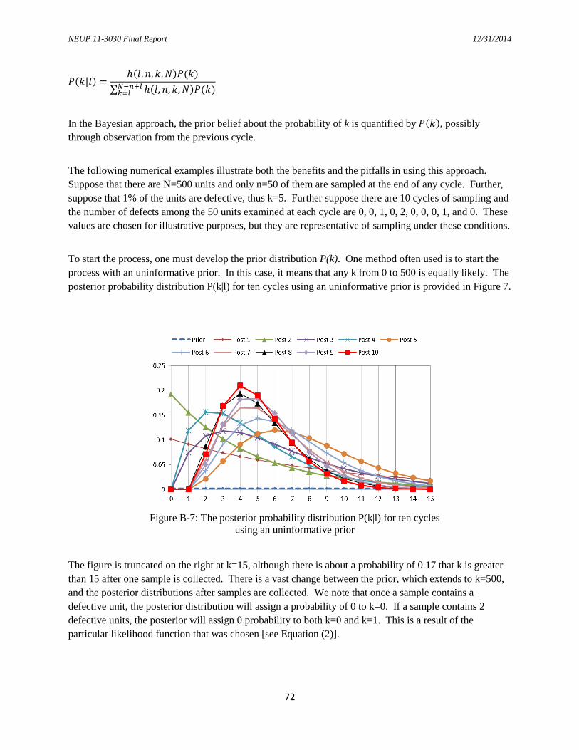
NEUP 11-3030 Final Report 12/31/2014
72
𝑃(𝑘|𝑙) =ℎ(𝑙, 𝑎, 𝑘, 𝑁)𝑃(𝑘)
∑ ℎ(𝑙, 𝑎, 𝑘, 𝑁)𝑃(𝑘)𝑁−𝑛+𝑎𝑘=𝑎
In the Bayesian approach, the prior belief about the probability of k is quantified by 𝑃(𝑘), possibly through observation from the previous cycle. The following numerical examples illustrate both the benefits and the pitfalls in using this approach. Suppose that there are N=500 units and only n=50 of them are sampled at the end of any cycle. Further, suppose that 1% of the units are defective, thus k=5. Further suppose there are 10 cycles of sampling and the number of defects among the 50 units examined at each cycle are 0, 0, 1, 0, 2, 0, 0, 0, 1, and 0. These values are chosen for illustrative purposes, but they are representative of sampling under these conditions. To start the process, one must develop the prior distribution P(k). One method often used is to start the process with an uninformative prior. In this case, it means that any k from 0 to 500 is equally likely. The posterior probability distribution P(k|l) for ten cycles using an uninformative prior is provided in Figure 7.
The figure is truncated on the right at k=15, although there is about a probability of 0.17 that k is greater than 15 after one sample is collected. There is a vast change between the prior, which extends to k=500, and the posterior distributions after samples are collected. We note that once a sample contains a defective unit, the posterior distribution will assign a probability of 0 to k=0. If a sample contains 2 defective units, the posterior will assign 0 probability to both k=0 and k=1. This is a result of the particular likelihood function that was chosen [see Equation (2)].
Figure B-7: The posterior probability distribution P(k|l) for ten cycles using an uninformative prior

NEUP 11-3030 Final Report 12/31/2014
73
Suppose that one has good prior information that the value of k is near 5, and there is low probability it is above 10. The posterior probability distribution P(k|l) for ten cycles using this high quality prior is provided in Figure 8. In this case, the prior is peaked near the correct value and the posterior distributions are also near the correct value.
Figure B-8: The posterior probability distribution P(k|l) for ten cycles
However, assume one choses a prior that is peaked around k=15, even though k=5. The posterior probability distribution P(k|l) for ten cycles using this low quality prior is provided in Figure 9. In this case, a large number of sampling cycles would be needed to get a posterior distribution peaked around the true value. In particular, as the prior assigns a probability of zero to any k, the posterior will always assign a probability of zero to this value of k, no matter what sample results are seen.
Other types of priors can be used. For example, one might wish to put a peak near the anticipated true value, but sit the peak on a base of an uninformative prior. The posterior probability distribution P(k|l)
Figure B- 9: The posterior probability distribution P(k|l) for ten cycles
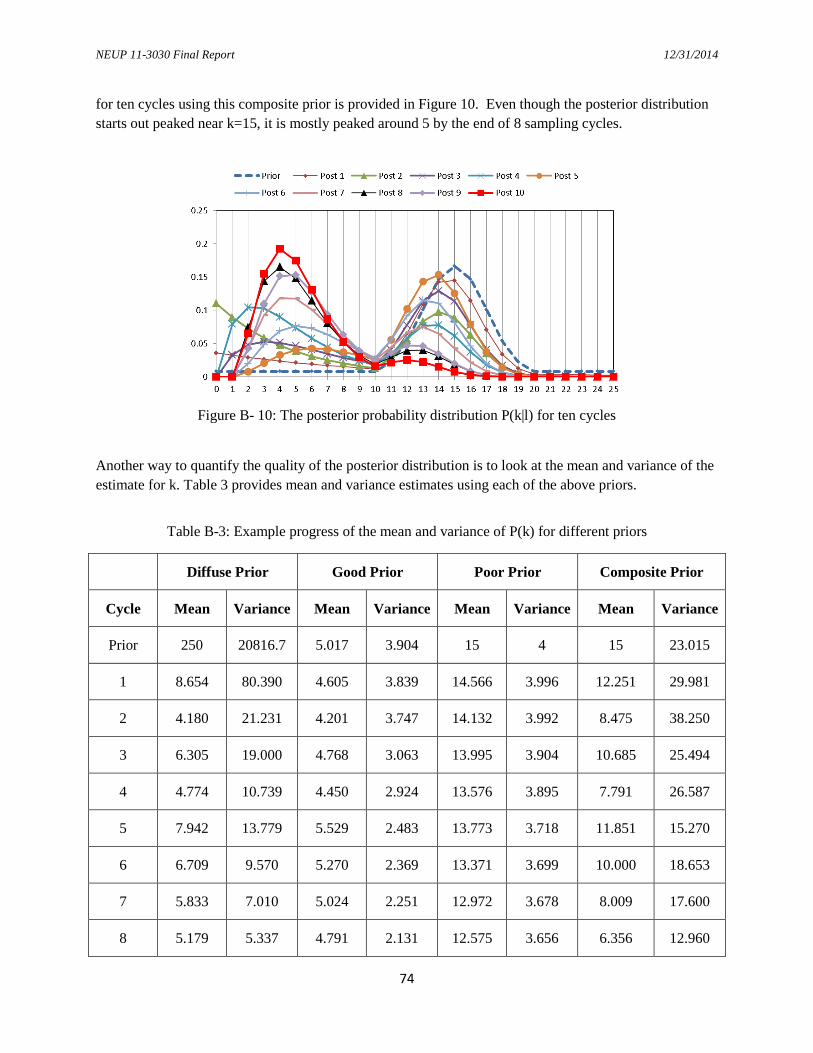
NEUP 11-3030 Final Report 12/31/2014
74
for ten cycles using this composite prior is provided in Figure 10. Even though the posterior distribution starts out peaked near k=15, it is mostly peaked around 5 by the end of 8 sampling cycles.
Another way to quantify the quality of the posterior distribution is to look at the mean and variance of the estimate for k. Table 3 provides mean and variance estimates using each of the above priors.
Table B-3: Example progress of the mean and variance of P(k) for different priors
Diffuse Prior Good Prior Poor Prior Composite Prior
Cycle Mean Variance Mean Variance Mean Variance Mean Variance
Prior 250 20816.7 5.017 3.904 15 4 15 23.015
1 8.654 80.390 4.605 3.839 14.566 3.996 12.251 29.981
2 4.180 21.231 4.201 3.747 14.132 3.992 8.475 38.250
3 6.305 19.000 4.768 3.063 13.995 3.904 10.685 25.494
4 4.774 10.739 4.450 2.924 13.576 3.895 7.791 26.587
5 7.942 13.779 5.529 2.483 13.773 3.718 11.851 15.270
6 6.709 9.570 5.270 2.369 13.371 3.699 10.000 18.653
7 5.833 7.010 5.024 2.251 12.972 3.678 8.009 17.600
8 5.179 5.337 4.791 2.131 12.575 3.656 6.356 12.960
Figure B- 10: The posterior probability distribution P(k|l) for ten cycles

NEUP 11-3030 Final Report 12/31/2014
75
9 5.582 5.341 5.015 2.066 12.488 3.560 6.851 12.797
10 5.070 4.308 4.801 1.962 12.105 3.532 5.706 8.704
There are potential benefits and difficulties in this method that should be explored with realistic data sets. If k is small and the fraction of units sampled is also small, then the updated P(k) will assign a higher and higher probability to k=0 for each cycle until the first defective unit is identified. This problem is magnified if the sampling technique does not detect every defective unit. The typical performance under three priors has been illustrated graphically and numerically. Other authors [8] explain these general types of results by saying that one obtains significant new information from the sampling only if one didn’t know much about the number of defects prior to beginning the sampling. These results also show that initial strong beliefs in the number of defects are modified only slowly by sampling results if they are wrong. As a general practice, one may desire that sampling data rather than prior information dominate the results after a number of samples have been taken. This philosophic bent may drive one to accept uninformative priors. The essential ingredient in the Bayes update step is the selection of the likelihood function, the function that relates sampled values to the statistical parameters. One might also consider incorporating aspects of both a physics model and sampled data in the likelihood function, either analytically or by using adjunct synthetic sampled data. For purposes of this discussion, we also assume that the probability of detection of an existing defect P(D) can be estimated, possibly using a Bayesian approach [9]. The probability that no defects are detected until a given cycle with the assumed example situation (N=500, n=50 and k=5) with perfection detection and a 40% detection rate is shown in Figure 11. The expected number of cycles until the first detection is made is 3.49 under the assumption of perfect detections and 5.07 when only 40% of the flaws present are detected. The information in Figure 11 is illustrative and similar calculations, possibly resulting in a family of curves, can be done prior to any real sampling. Such numerical exercises could help in determining when an approach might be expected to result in data useful for setting or adjusting transition rates between states in a physics-based multi-state degradation model.

NEUP 11-3030 Final Report 12/31/2014
76
Let Pi(k) denote the probability that k defective units have been detected by the end of cycle i. Knowledge of how many defects occurred during cycle i might be useful in updating the values for b and β in the rate equation for 𝜙1. The number of defects is not actually known, but in a symbolic sense, letting 𝑁𝐷𝑖 denote the accumulated number of defects detected by the end of cycle i, (𝑁𝐷𝑖 − 𝑁𝐷𝑖−1) 𝑃(𝐷)⁄ represents the number of defects that occurred during cycle i. In a numerical sense, the probability distribution on this quantity can be evaluated using Monte Carlo techniques, given knowledge of Pi-1(k), Pi(k) and P(D). Low values of P(D) may cause high variability in this calculation. Also assume the inspection cycle length T is short enough that the probability of defect formation in a specific unit during the cycle can be approximated by 𝑝 = 𝑇(𝑏/𝛽)(𝑇/𝛽)𝑏−1. Because there are N units in the system that each have the same probability of forming a defect during this cycle, the probability that x of them form defects during cycle T can be expressed as a binomial distribution,
𝑃(𝑋 = 𝑥) = �𝑁𝑥 � 𝑝𝑚(1 − 𝑝)𝑁−𝑚
for x=0, 1, …, N. This binomial distribution has mean value Np and variance Np(1-p). One possible way to choose values for b and β in the rate equation 𝜙1 is to use a Monte Carlo technique that evaluates the mean and variance of the symbolic quantity (𝑁𝐷𝑖 − 𝑁𝐷𝑖−1) 𝑃(𝐷)⁄ and equates those values to the mean and variance of the binomial distribution. The values b and β can be adjusted every inspection cycle because P(k) is updated every cycle. The process starts with an initial prior distribution P0(k)=P(k). The posterior distribution at the end of a cycle can be used as the prior distribution for the next cycle.
Figure B-11: Probability that no defects are detected until a given cycle with N=500, n=50 and k=5 with perfection detection and a 40% detection rate
NEUP 11-3030 Final Report 12/31/2014
77
In general, the approach of equating means and variances results in two equations involving the two unknown values b and β that could be solved using established numerical techniques. However, because N is known, and the mean and variance of the binomial distribution both depend on p, the variance can be determined from the mean value. Thus, one can determine only one of b and β. However, one could update both of them, holding the other one fixed, and determine whether the initial values of either, or both, were stable under the updating process. If not, that would indicate that further work might be needed to reliably fit the rate equation. The approach outlined here for selecting values for b and β in the rate equation 𝜙1 uses an implicit assumption that all units are of the same age. The approach can be generalized when some of the units have been replaced if the inspection process can identify which units have been replaced. Consider the situation where N1 units were replaced at a known time, thus the original N units have been divided into two subsets N1 and N2 where N=N1+N2. Each subset would then be tracked separately and would potentially have different values of b and β. CONCLUSIONS In short, NDE methods for the detection of crack precursors offer the promise of informing pertinent aspects of a multi-state degradation process. This process, a semi-Markovian approach to address crack initiation and growth in system piping, has the advantage that while it is capable of accounting for cumulative damage as the heartbeat framework does and is compatible with the anticipated New Generation System Code (NGSC) structure, it can be also used to augment existing PRAs with regard to passive component failures using legacy codes. As such, concepts explored in this paper directly support the NEUP project objective of developing a methodology that addresses multiple aging mechanisms involving large numbers of components in a computationally feasible manner, where the sequencing of events is conditioned on the physical conditions predicted in a simulation environment. In this paper, promising methods for the detection of crack precursors in metals were reviewed and assessed to evaluate the advantages and disadvantages of each method, including their detection capability and associated sources of uncertainty. Additionally, a framework for integrating these methods into a PRA and plant surveillance program was explored. Although the potential of this framework to address the impact of aging effects on risk and for quantifying the effectiveness of aging management strategies in maintaining safety margins is encouraging, the potential benefits (and complications) should be evaluated further using realistic data sets and considering in more detail the feasibility of using the select NDE methods in real-world applications. However, before such a framework could be fully implemented, several areas of future research are suggested, including but necessarily limited to:
• The feasibility of implementing NDE methods under real-world applications for detection of crack precursors, including a refined understanding of their associated probabilities of detection,
• The integration or reconciliation of insights obtained from sampling data gathered from surveillance programs and those derived from physics-based degradation models, and

NEUP 11-3030 Final Report 12/31/2014
78
• The validation of the proposed methods with realistic data sets. This additional research would ultimately yield a better understanding of the advantageous economics of early precursor detection and allow cost-benefit analyses of new detection techniques to be developed.
NEUP 11-3030 Final Report 12/31/2014
79
REFERENCES
1. Stephen D. Unwin, et al., Physics-Based Stress Corrosion Cracking Component Reliability Model cast in an R7-Compatible Cumulative Damage Framework, PNNL-20596, July 2011.
2. G. Sposito, et al., A Review of Non-Destructive Techniques for the Detection of Creep Damage in Power Plant Steels, NDT&E International 43 (2010) 555–567.
3. Pradeep Ramuhalli, et al., A Bayesian Prognostic Algorithm for Assessing Remaining Useful Life of Nuclear Power Components, NPIC&HMIT 2010, November 7-11, 2010, Las Vegas, Nevada.
4. Pradeep Ramuhalli, et al., An Assessment of Uncertainty in Remaining Life Estimation for
Nuclear Structural Materials, Eighth American Nuclear Society International Topical Meeting on Nuclear Plant Instrumentation, Control and Human-Machine Interface Technologies NPIC&HMIT 2012, July 22-26, 2012, San Diego, California.
5. Pradeep Ramuhalli, et al., Nondestructive Examination (NDE) Detection and Characterization of
Degradation Precursors, PNNL-21692, September 2012.
6. RM Meyer, et al., Materials Degradation and Detection (MD2): Deep Dive Final Report, PNNL-22309, Revision 0, February 2013.
7. RM Meyer, et al., Technical Needs for Prototypic Prognostic Technique Demonstration for Advanced Small Modular Reactor Passive Components, PNNL-22488, Revision 0, May 2013.
8. G. Roussel, L. Cizelj, “Reliability of Sampling Inspection Schemes Applied to Replacement Steam Generators,” Journal of Pressure Vessel Technology, Vol. 129 pp.109-11, (2007).
9. Barnier, M., P. Pitner and T. Riffard, “Estimation of crack size distribution from in-service
inspection data for the calculation of failure probabilities,” European Safety and Reliability Conference, Copenhagen, (1992).