microfluidic networking: modelling and analysis
TRANSCRIPT

MICROFLUIDIC NETWORKING: MODELLING AND
ANALYSIS
RELATORE: Ch.mo Prof. Andrea Zanella
LAUREANDO: Andrea Biral
A.A. 2012-2013

UNIVERSITA DEGLI STUDI DI PADOVA
DIPARTIMENTO DI INGEGNERIA DELL’INFORMAZIONE
TESI DI LAUREA MAGISTRALE IN INGEGNERIA DELLE
TELECOMUNICAZIONI
MICROFLUIDIC NETWORKING:
MODELLING AND ANALYSIS
RELATORE: Ch.mo Prof. Andrea Zanella
LAUREANDO: Andrea Biral
Padova, 10 dicembre 2012


Abstract
Droplets microfluidics refers to manipulation and control of little amounts of flu-
ids flowing into channels of micro-scale size. Our aim, pursued in the present
thesis, is to design a network formed by such microchannels and define a model
to properly route the droplets inside them. However, this kind of study relies on
the preliminary deep knowledge of microfluidic flow dynamics and typical prop-
agation characteristics. Accordingly, we begin our dissertation by introducing
the physical laws that govern microfluidics. Then, we discuss the current under-
standings about droplets formation, transport and their behavior in bifurcating
channels, corroborating all with simulative results. Furthermore, we show how
such concepts can be integrated in our networking solution and, lastly, we imple-
ment a microfluidic network with bus topology and illustrate its performance.


Contents
1 Introduction 1
2 Basic microfluidic concepts 5
2.1 Viscosity . . . . . . . . . . . . . . . . . . . . . . . . . . . . . . . . 5
2.2 Capillary number . . . . . . . . . . . . . . . . . . . . . . . . . . . 6
2.3 Reynolds number . . . . . . . . . . . . . . . . . . . . . . . . . . . 7
2.4 Laminar flow . . . . . . . . . . . . . . . . . . . . . . . . . . . . . 8
2.5 Hagen-Poiseuille’s law . . . . . . . . . . . . . . . . . . . . . . . . 9
2.6 Rayleigh-Plateau instability . . . . . . . . . . . . . . . . . . . . . 12
2.7 Analogy between fluidic and electric circuit . . . . . . . . . . . . . 13
3 Droplet generation 21
3.1 Breakup in co-flowing streams . . . . . . . . . . . . . . . . . . . . 21
3.2 Breakup in elongational strained flows . . . . . . . . . . . . . . . 22
3.3 Breakup in cross-flowing streams . . . . . . . . . . . . . . . . . . 24
3.3.1 Forces anlysis . . . . . . . . . . . . . . . . . . . . . . . . . 25
3.3.2 Squeezing regime . . . . . . . . . . . . . . . . . . . . . . . 28
3.3.3 Dripping regime . . . . . . . . . . . . . . . . . . . . . . . . 36
4 Characterization of droplet dynamics in a bifurcating channel 39
4.1 Droplet breakup in a bifurcating channel . . . . . . . . . . . . . . 39
4.1.1 Breakup regime . . . . . . . . . . . . . . . . . . . . . . . . 40
4.1.2 Non-breakup regime . . . . . . . . . . . . . . . . . . . . . 41
4.1.3 Simulations and numerical results . . . . . . . . . . . . . . 44
4.2 Regulation of droplet traffic in a T-junction . . . . . . . . . . . . 45
4.2.1 Simulative example . . . . . . . . . . . . . . . . . . . . . . 47
iii

CONTENTS
5 Design and performance of a microfluidic bus network 51
5.1 Mechanism for droplet routing . . . . . . . . . . . . . . . . . . . . 51
5.2 Bus network dimensioning . . . . . . . . . . . . . . . . . . . . . . 53
5.2.1 Mathematical and physical constraints . . . . . . . . . . . 56
5.3 Bus network performance . . . . . . . . . . . . . . . . . . . . . . 64
5.3.1 Numerical results . . . . . . . . . . . . . . . . . . . . . . . 67
6 Future developments 73
6.1 Scheduling . . . . . . . . . . . . . . . . . . . . . . . . . . . . . . . 73
6.2 Network topology . . . . . . . . . . . . . . . . . . . . . . . . . . . 74
A OpenFOAM 77
Bibliography 79
iv

Chapter 1
Introduction
Microfluidic is both a science and a technology that deals with the control of small
amounts of fluids flowing through microchannels. These have dimension in the
order of micrometers and are usually fabricated in PDMS, i.e., Polydimethylsilox-
ane, which is a silicon based organic polymer. In this thesis we are specifically
interested in droplets microfluidics which is a science related to the control of
the motion dynamics of droplets in such microchannels. In this scenario, small
drops are dispersed into another fluid, which is immiscible with them; this is why
in literature they are conventionally called dispersed phase, while the immiscible
substance in which they are immersed is called continuous phase.
This line of reserch has emerged strongly in the past few years but the field
is still at an early stage of development. Nevertheless its capabilities and advan-
tages are already well known. The so called droplet microfluidics technology, in
fact, exploits both its most obvious characteristic (small size) and less obvious
characteristics of fluid in microchannels (such as laminar flow) to provide new
capabilities in the control and concentrations of molecules in space and time.
Moreover it has the potential to influence many subject areas from chemical syn-
thesis and biological analysis to optics and information technology.
Nowadays, applications of microfluidics span from inkjet printheads to DNA
chips, from micro-propulsion to micro-thermal technologies. However, the most
promising utilization of microfluidic technologies have just been in analysis, for
which they offer a number of useful capabilities: the ability to use very small
quantity of samples and reagents and to carry out separations and detections
with high resolution and sensitivity, low cost, short time for analysis and small
1

1. INTRODUCTION
footprint for the analytical devices. All these advantages however come at the
price of raise a new set of fluid dynamical problems that appear due to the de-
formable interface of the droplets, the need to take into account interfacial tension
and its variations, and the complexity of singular events such as splitting drops.
In the physicist’s vocabulary, droplets introduce nonlinear laws into the otherwise
linear Stokes flows. Evidence of this nonlinearity can be found, for instance, by
considering that different flow regimes can appear in the same channel and under
similar forcing conditions. These transitions between widely different behaviors
are possible because modifications in the drop geometry couple back to the flow
profiles and amplify initially small variations. A large body of work has recently
attempted to tackle these fluid dynamical questions, leading along the way to cre-
ative new design for microfluidic devices -e.g., Labs-on-a-Chip (see Figure 1.1)-
and new physical approaches to control the behavior of drops.
Figure 1.1: Example of Lab-on-a-chip: a microfluidic chemostat used to study the
growth of microbial populations.
In the future, one may envision microfluidic systems with mazes of microchan-
nels along which droplets conveying solutes, materials and particles undergo
transformations and reactions. These devices could be used to perform all sort of
bio-/physiochemical analysis or to produce novel entities by means of specific “mi-
crofluidic machines” able to process fluids at such a scale. This particular scenario
2
has inspired the following work. Indeed, our idea is to create a network, consisting
of microchannels, in order to connect with each other more microfluidic machines.
In this way, we could miniaturize and automate in a single device an entire labora-
tory gaining, at the same time, in versatility and flexibility. In fact, once a specific
microfluidic machine has opportunely processed an incoming droplet, the latter
might be reinjected in the network to reach another target microfluidic machine
undergoing further transformations and so on. Moreover, we could parallelize
the tasks undertaken by different microfluidic machines obtaining a consequent,
significant time saving. Such a prospective requires, however, preliminarily, the
control over elementary operations like droplet production, breakup, transport
and redirection. This motivated us to structure the present thesis as described
below.
In Chapter 2 we introduce the main underlying concepts of droplets microflu-
idics in order to let the reader familiarize with the notation and the physical
ingredients typical of this science.
Chapter 3, instead, is dedicated to the study of droplet production in mi-
crochannels. In particular, it contains a brief review of the three main approaches
proposed, in this regard, in literature with a particular focus on the solution that
satisfy our requirements the most. Furthermore, here we also present a set of
simulative results obtained with the CFD software OpenFOAM (see Appendix
A) in order to validate the theoretical basis introduced.
In the first half of Chapter 4 we treat the dynamics of droplet breakup in a
junction. The latter is, of course, a founding part of our microfluidic network
since it is an indispensable element to direct the droplets to the various target
microfluidic machines. This topic is very important to us because we need to
preserve the integrity of the droplets throughout the entire network and, thus,
even when they face “sensitive points” like bifurcations. Therefore, here, we’ll
analyze in details the conditions that allow us to transport droplets avoiding their
splitting in the channels’ ramifications.
Then, in the second part of the chapter, we present a model for the pro-
grammable partitioning of droplets at a T-junction illustrating how we can direct
3
1. INTRODUCTION
them in the desired branch of the bifurcation. Once again, we corroborate our
conclusions with corresponding numerical simulations obtained at the calculator.
In Chapter 5 we finally introduce a microfluidic bus-shaped network, discuss
the mathematical and physical constraints that we need to respect in order to
correctly dimension it and then illustrate the performance of such a system.
Lastly, Chapter 6 focuses on the possible future developments of the thesis,
anticipating eventual improvements and alternative solutions.
4

Chapter 2
Basic microfluidic concepts
The present chapter is intended to give an overview of the microfluidic’s physical
basis by collecting and describing the main parameters and models which rule
fluid transport and droplet dynamics in microfluidic systems. Thus, the aim
of this section is to allow the reader to familiarize with the principal concepts
of microfluidic that will be recalled and further analyzed throughout the entire
work.
2.1 Viscosity
Viscosity is a measure of the resistance of a fluid which is being deformed by
either shear stress or tensile stress. In simple terms, it describes a fluid’s internal
resistance to flow and may be thought of as a measure of fluid friction: the greater
the viscosity, the greater its resistance to flow and vice versa. With the exception
of superfluids, all real fluids have some resistance to stress and therefore are
viscous. In common usage, a liquid with a viscosity less than water is known as
mobile liquid while, in the opposite case, it is called viscous liquid. Synthetically,
the physical behavior associated with viscosity can be described as follows: in any
flow, molecule’s layers move at different velocities and the fluid’s viscosity arises
from the shear stress between the layers that ultimately opposes any applied
force. The relationship between the shear stress and the velocity gradient can be
obtained by considering two plates closely spaced at a distance y, and separated
by a homogeneous substance. Assuming that the plates are very large, with a
large area A, such that edge effects may be ignored, and that the lower plate
5
2. BASIC MICROFLUIDIC CONCEPTS
is fixed, let a force F be applied to the upper plate. If this force causes the
substance between the plates to undergo shear flow with a velocity gradient u/y,
it results:
F = µAu
y, (2.1)
where µ[Pa · s] is the proportionality factor called dynamic viscosity. It should
be noted that viscosity is a function of temperature: fluid become less viscous
as temperature increases. In this thesis, however, we assume the temperature
is constant during the operation of microfluidic devices. Water at 20 has a
characteristic dynamic viscosity of 1.002 · 10−3Pa · s.Equation (2.1) can also be expressed in terms of shear stress (τ = F
A). In
particular, as reported in differential form by Isaac Newton for straight, parallel
and uniform flow, the shear stress between layers is proportional to the velocity
gradient in the direction perpendicular to the layers: τ = µ∂u∂y. Newton’s law
of viscosity, given above, is a constitutive equation which holds for the so called
Newtonian fluids. Non-Newtonian fluids, instead, exhibit a more complicated
relationship between shear stress and velocity gradient than simple linearity. The
analysis of the latter, however, is beyond the scope of this work since we will be
dealing only with Newtonian fluid.
Finally, in many situations we are concerned with the ratio between the dy-
namic viscosity and the density of the fluid: ν = µρwhich is a coefficient named
kinematic viscosity. The SI physical unit of ν is [m2/s]. Water at 20 has a
characteristic dynamic viscosity of about 10−6m2/s.
2.2 Capillary number
In fluid dynamics, the Capillary number represents the relative magnitude of
viscous forces versus surface tension acting across an interface between a liquid
and a gas, or between two immiscible liquids. It is a dimensionless parameter
defined as:
Ca =µu
σ(2.2)
where µ[Pa · s] is the viscosity of the main liquid, u[m/s] is its mean velocity
and σ[N/m] is the surface or interfacial tension coefficient between the two fluid
phases.
6

2.4 REYNOLDS NUMBER
With reference to the droplet microfluidic context:
Ca =µcuc
σ(2.3)
where µc[Pa ·s] is the viscosity of the carrier fluid in which droplets are immersed,
uc[m/s] is its mean velocity and σ[N/m] is the interfacial tension coefficient be-
tween continuous and dispersed phase.
Since viscous stress represents a destructive force while interfacial tension
acts as a cohesive force, Capillary number may be thought of as a measure of
the cohesion of the droplet: the greater is the Capillary number, the greater the
probability of droplet splitting and vice versa.
2.3 Reynolds number
In fluid dynamics the Reynolds number is a dimensionless parameter that gives a
measure of the ratio of inertial forces to viscous forces and consequently quantifies
the relative importance of these two types of forces for given flow conditions.
Reynolds numbers frequently arise when performing dimensional analysis of
fluid dynamics problems, and as such can be used to determine dynamic simil-
itude between different experimental cases. They are also used to characterize
different flow regimes, such as laminar or turbulent flow: laminar flow (see Section
§2.4) occurs at low Reynolds numbers, where viscous forces are dominant, and
is characterized by smooth, constant fluid motion; turbulent flow occurs at high
Reynolds numbers and is dominated by inertial forces, which tend to produce
chaotic eddies, vortices and other flow instabilities.
Mathematically, Reynolds number is defined as follows:
Re =ρuL
µ(2.4)
where µ[Pa·s] is the viscosity of the liquid, u[m/s] is its mean velocity, ρ[kg/m3] is
its density and L[m] is a characteristic linear dimension of the system. Declining
it in the microfluidic context, L is conventionally considered equal to the hydraulic
diameter of the channel (DH = 4A/P , where A is the cross sectional area of the
channel and P is the wetted perimeter of the channel), µ is the viscosity of the
carrier liquid (µc), u is its mean velocity (uc) and ρ is its density (ρc). Thus:
Re =4Aρcuc
Pµc
(2.5)
7

2. BASIC MICROFLUIDIC CONCEPTS
2.4 Laminar flow
In fluid dynamics, laminar flow, sometimes known as streamline flow, is a flow
regime characterized by high momentum diffusion and low momentum convection
that involves a very orderly motion of fluid’s particles which are organized in
parallel layers (or laminae). Although all the molecules move in straight lines,
they are not all uniform in velocity: if the mean velocity of the flow is u, then
the molecules at the centre of the tube are moving at approximately 2u, whilst
the molecules at the side of the tube are almost stationary. Moreover, in this
regime, the fluid tends to flow without lateral mixing, there are no cross currents
perpendicular to the direction of flow, nor eddies or swirls of fluids.
This kind of behavior occurs as long as the Reynolds number (see Section §2.3)
is below a specific critical value ReCR ≃ 2000 that depends on the particular flow
geometry and can be sensitive to disturbance levels and imperfections present in
a given configuration. Bearing in mind this condition, laminar flow is exactly
the regime we would expect to see in typical microfluidic systems since their
characteristic small length-scales (L ≃ 10−6m) and slow fluid velocities (u ≃10−3m/s) lead to very low Reynolds number (Re = ρuL
µ≃ 10−3).
Further, when Reynolds number is much less than 1, which is the case of our
competence, creeping motion (or Stokes flow) occurs. This is an extreme case
of laminar flow where viscous (friction) effects are much greater than inertial
forces. This physical phenomenon entails two additional interesting properties in
incompressible Newtoninan fluids:
Instantaneity: a Stokes flow has no dependence on time other than through
time-dependent boundary conditions. This means that, given the boundary
conditions of a Stokes flow, the flow can be found without knowledge of the
flow at any other time;
Time-reversibility: a time-reversed Stokes flow solves the same equations
as the original Stokes flow. Practically, it implies that it is difficult to mix
two fluids using creeping flow.
8

2.5 HAGEN-POISEUILLE’S LAW
2.5 Hagen-Poiseuille’s law
In fluid dynamics, the Hagen-Poiseuille equation is a physical law that relates the
pressure drop in a fluid flowing through a long pipe with its volumetric flow rate.
The assumptions of the equation are that the fluid is viscous and incompressible,
the flow is laminar through a channel of constant cross-section and there is no
acceleration of fluid. These hypotheses, as we already pointed out, are fully
satisfied in the typical microfluidic systems.
Now, in order to derive Hagen-Poiseuille’s law, let’s begin considering the
incompressible Navier-Stokes equation for uniform-viscous Newtonian fluids with
no body forces:
ρ∂u
∂t= −ρu∇u−∇p+ µ∇2u (2.6)
where u [m/s] is the velocity field, which is the description of the velocity of the
fluid at a given point in space and time, and is denoted by u = u(r, t), where r [m]
is a position vector specifying a location in space and t [s] is time; ρ [kg/m3] is the
fluid density; µ [Pa · s] is the dynamic viscosity and p [Pa] is the pressure. More
specifically, in Equation (2.6), ρ∂u∂t
represents the rate of change of momentum,
−ρu∇u concerns convective force, −∇p describes the pressure force while viscous
force is indicated in the term µ∇2u.
Let’s then consider a long cylindrical channel with the x-direction along the
axis of the channel. In the steady-state of fully developed fluid flow in the channel,
its velocity field is unidirectional and laminar and there is no acceleration of the
fluid. Thus, the unsteady and convection terms are all zero, and Equation (2.6)
becomes:
∇p = µ∇2u (2.7)
Equation (2.7) highlights the balance between the net pressure force and the net
viscous force. Due to the geometric simplifications and the boundary conditions
(u = 0 at r = R), the pressure driven motion, named Poiseuille flow, in the
circular channel of radius R [m] is parabolic across the diameter:
u =R2 − r2
4µ
(−dp
dx
)= umax
(1− r2
R2
)(2.8)
where umax is the maximum velocity: umax = R2
4µ
(− dp
dx
)at r = 0. The Poiseuille
flow is characterized by a parabolic velocity profile (see Figure 2.1): the velocity
of flow in the center of the channel is greater than that toward the outer walls.
9

2. BASIC MICROFLUIDIC CONCEPTS
In contrast, electrically driven flow that is a useful alternative to pressure-driven
flow of water, known as electro-osmotic flow (EOF), offers a flat velocity profile
across the channel. The next step requires the calculation of the total volumetric
u
r
x
r=R
r=-R
Figure 2.1: Parabolic velocity profile of the Poiseuille flow.
flow rate Q [m3/s] in the circular channel. In order to get it, we need to spacially
integrate the velocity contributions (Equation (2.8)) from each lamina. Accord-
ingly, the volumetric flow rate for the steady-state pressure-driven fluid flow in
the channel, described by the Hagen-Poiseuille’s law, becomes:
Q =πR4
8µ
(−dp
dx
). (2.9)
Normalizing Equation (2.9) by the cross-sectional area, we generate the area-
averaged velocity U [m/s]:
U =Q
πR2=
R2
8µ
(−dp
dx
). (2.10)
To be precise, the Hagen-Poiseuille’s law applies only for a channel that is per-
fectly straight and infinitely long. However, we can reasonably apply Equation
(2.9) even to a channel with finite length L [m] as long as this is by far the
prevalent dimension of the geometry.
For most pressure-driven microfluidic devices, we can assume that the pressure
gradient along the channel length is uniform. Then, we can approximate the term
− dpdx
to ∆pL, where ∆p [Pa] is the pressure difference through a finite channel length
L. With this approximation, Equation (2.9) becomes simply:
Q =πR4
8µ
∆p
L(2.11)
where Q is defined as positive for flow from inlet to outlet.
10

2.5 HAGEN-POISEUILLE’S LAW
Equation (2.11) gives the flow-pressure relation in pressure-driven channels
and can be simplified as:
Q =∆p
RH
(2.12)
where the hydraulic resistance RH [Pas3/m] is defined, for a cylindrical tube, as:
RH =8µL
πR4. (2.13)
In general, Equation (2.13) can be applied for non-circular channels, by replacing
the channel radius R with the hydraulic radius rH or diameter DH = 2rH . The
hydraulic radius of the channel rH [m] is a geometric constant defined as rH = 2AP,
where A [m2] is the cross-sectional area of the channel and P [m] is the wetted
perimeter.
In microfluidic networks, most channel geometries are rectangular. For a
rectangular microchannel with a low aspect ratio (w ≈ h), the reciprocal of the
hydraulic radius becomes the sum of the reciprocals of the channel width w [m]
and the channel height h [m]: 1/rH = 1/w+ 1/h or rH = wh/(w+ h). However,
this estimate gives about 20% error and thus it isn’t much satisfying.
Actually, the solution to Equation (2.7) for a rectangular channel is quite
complicated to derive, and it can be only calculated exactly as the summation
of a Fourier series. The hydraulic resistance for the rectangular microchannel, in
fact, is given by:
RH =12µL
wh3(1− h
w
(192π5
∑∞n=1
1(2n−1)5
tanh(
(2n−1)πw2h
))) . (2.14)
Note that when the aspect ratio is high1 (h/w < 1), the Fourier series can be
truncated at the first harmonica (n = 1 in Equation (2.14)) since the other terms
become negligible and we obtain the simplified formula:
RH =12µL
wh3
[1− 192h
π5wtanh
(πw2h
)]−1
. (2.15)
This Equation is accurate to within 0.26% for any rectangular channel that haswh< 1, provided that the Reynolds number Re is below 103.
Finally, by reversing Equation (2.12) and combining it with Equation (2.15),
it results:
∆p =12µLQ
wh3
[1− 192h
π5wtanh
(πw2h
)]−1
. (2.16)
1This condition is always verified in the microfluidic systems we considered.
11

2. BASIC MICROFLUIDIC CONCEPTS
which is the Hagen-Poiseuille’s law we’ll use hereafter to describe the flow in our
rectangular microfluidic channels.
2.6 Rayleigh-Plateau instability
Rayleigh-Plateau instability explains why and how a falling stream of fluid breaks
up into smaller drops. The driving force of the process arises from the intrinsic
tendency of the liquids to minimize their surface area.
The explanation of this instability begins with the existance of tiny perturba-
tions in the surface of the liquid. These are always present, no matter how smooth
the stream is. If the perturbations are resolved into sinusoidal components, the
equation for the radius of the stream can be written as: r(z) = r0 + Akcos(kz),
where r0 is the radius of the umperturbated stream, Ak is the amplitude of the
perturbation, z is the distance along the axis of the stream and k is the wave
number (a measure of how many peaks and troughs per meter are present in the
liquid surface). We thus find that some components grow with time while others
decay with time. Among those that grow with time, some grow at faster rates
than others. Whether a component decays or grows, and how fast it grows is
entirely a function of its wave number k and the radius of the original cylindrical
stream r0.
By assuming that all possible components exist initially in roughly equal (but
minuscule) amplitudes, the size of the final drops can be predicted by determining,
through wave number, which component grows the fastest. As time passes, in
fact, the component whose growth rate is maximum will come to dominate and
will eventually be the one that pinches the stream into drops.
We observe that at the troughs the radius of the stream is smaller, hence,
according to the Young-Laplace equation reported below, the pressure due to
surface tension is increased:
∆p = σ(1
r1+
1
r2) (2.17)
where σ is the so called surface tension coefficient, r1 is the radius of the stream
and r2 is the curvature of the sinusoidal wave describing the liquid surface profile.
Likewise, at the peaks the radius of the stream is greater and, by the same
reasoning, pressure due to surface tension is reduced.
12

2.7 ANALOGY BETWEEN FLUIDIC AND ELECTRIC CIRCUIT
If this were the only effect, we would expect that the higher pressure in the
trough would squeeze liquid into the lower pressure region in the peak, under-
standing how the wave grows in amplitude with time. But the Young-Laplace
equation is influenced by two separate radius coponents. In this case, one is the
radius, already discussed, of the stream itself (r1). The other is the radius of the
curvature of the wave (r2). Observe that the radius of curvature at the trough is
negative meaning that, according to Yoiung-Laplace, it decreases the pressure in
the trough. Likewise, the radius of curvature at the peak is positive and increases
the pressure in that region. The effect of these components is in opposite with
the action of the radius of the stream itself. The two phenomena, in general,
do not exactly cancel. One of them will have greater magnitude than the other,
depending upon wave number k and the initial radius of the stream r0. In par-
ticular, when the wave number is such that the radius of curvature of the wave
dominates the stream’s one, such components will decay over time. Conversely,
when the radius of the stream dominates the wave’s curvature, such components
grow exponentially with time and promote drops formation.
When all the math is done, it can be found that unstable components (ie, the
components that grow over time) are only those where the product of the wave
number with the initial radius is less than unity: kr0 < 1.
2.7 Analogy between fluidic and electric circuit
It is quite intuitive to consider the flow of a fluid like the flow of electricity: indeed,
the molecules of fluid in a hydraulic circuit behave much like the electrons in an
electrical circuit. On this purpose, the present Section is intended to highlight
the main physical similarities between microfluidic circuits and electric circuits,
mapping the electric circuit elements and theory onto corresponding microfluidic
circuit elements and models. This well-known hydraulic-electric circuit analogy
can be straightforwardly used to prescribe the flow/pressure relation in complex
microfluidic networks based on conventional electric circuit theory. Starting from
the basics, in electronics, linear resistors are the simplest circuit element and their
resistance RE[Ω] is predetermined by physical parameters:
RE =ρEL
A(2.18)
13

2. BASIC MICROFLUIDIC CONCEPTS
where ρE[Ωm] is the reisistivity of the conductor, L[m] is the length of the con-
ductor and A[m2] is its cross-sectional area (see Figure 2.2(a)). The resistance of
the resistors can be prescribed by Ohm’s law:
V = REI (2.19)
where V [V ] is the voltage across the conducting material and I[A] is the current
flowing through the conductor (see Figure 2.2(b)). This formulae and relations
between voltage, current, electric resistance and conductor length are physically
similar to those between pressure, flow, hydraulic resistance and channel length
in a microfluidic context. In particular, Ohm’s law (Equation (2.19)) finds its
counterpart in the so called Hagen-Poiseuille’s law (see Section §2.5):
∆p = RHQ (2.20)
where ∆p[Pa] is the pressure difference across a microfluidic channel, Q[m3/s]
is the volumetric flow rate that crosses the channel and RH [Pa · s/m3] is the
hydraulic resistance (see Figure 2.2(d)). Since we are interested in microfluidic
channels of rectangular cross-section, the approximated formula for the hydraulic
resistance to which we have to refer is the following:
RH =aµL
wh3(2.21)
where L[m] is the length of the channel, w[m] is the width of the channel, h[m]
is the height of the channel and a is a dimensionless parameter defined as a =
12[1− 192hπ5w
tanh(πw2h)]−1 (see Figure 2.2(c)).
Continuing with the electric circuit analogy, if N fluidic resistors (microfluidic
channels) are collectively arranged in series, an equivalent single fluidic resistor
has a hydraulic resistance equal to the sum of the N hydraulic resistances:
RH,s = RH,1 +RH,2 + ...+RH,N . (2.22)
This is due to series-connected fluidic resistors carrying the same volumetric flow
from one terminal to the other. Similar simplification can be applied to parallel-
connected fluidic resistors. In a circuit containing N fluidic resistors in parallel,
the equivalent single fluidic resistor has a hydraulic resistance equal to the recip-
rocal of the sum of reciprocals of each hydraulic resistance:
RH,p = RH,1 ∥ RH,2 ∥ ... ∥ RH,N
RH,p =1
1RH,1
+ 1RH,2
+...+ 1RH,N
.(2.23)
14

2.7 ANALOGY BETWEEN FLUIDIC AND ELECTRIC CIRCUIT
L
A electric resistor
(a)
I
RE
V+ V-
(b)
L
w
h
microfluidic channel
(c)
Q
RH
p+ p-
(d)
Figure 2.2: Physical similarities between the flow of a fluid in a rectangular mi-
crochannel and the flow of electricity in a resistor.
Another very useful fluidic/electric similarity concerns sources. Most pressure-
driven microfluidic devices, in fact, need to be powered using external pressure
sources. Conventionally, external pumps such as syringe and peristaltic pumps
are widely used to supply constant fluid flow to devices. The volumetric flow
supplied by the pumps is completely independent of the pressure drop across
the inlet and outlet ports of a device. It cannot be known a priori the pressure
drop across an independent fluid flow source, because it depends entirely on the
equivalent hydraulic resistance of the circuit to which it is connected. In this case,
an independent constant fluid flow source QS is analogous to an independent DC
current source. Actually, in order to introduce the intrinsic non-ideality of the
sources, we need also to consider an internal resistance ri ≫ in parallel to the
ideal current generator (see Figure 2.3).
riQS
Figure 2.3: Analogy between constant fluidic flow source and current generator.
15

2. BASIC MICROFLUIDIC CONCEPTS
An alternative method is to connect an independent pressure source to in-
let ports. Basically, the flow is controlled by the gravity-driven flow induced
by the hydraulic head difference, ∆h[m], between the vertical source-inlet and
drain-outlet reservoirs of microfluidic devices. For an independent and constant
pressure source, ∆h has to be held constant all the time. Alternatively, pres-
surized reservoirs connected with external pneumatic sources are used to provide
independent, constant and controllable pressure to a device. The independent
constant pressure source pS is analogous to the corresponding independent DC
voltage source. In this case the intrinsic non-ideality of the source is rendered
once we add a series internal resistance ri ≪ to the ideal voltage generator (see
Figure 2.4).
ri
ΔpS
+
-
Figure 2.4: Analogy between constant fluidic pressure source and voltage genera-
tor.
Most microfluidic network-based devices, however, are fed with two or more
pumping sources for the source-inlet ports (for example, continuous phase and
dispersed phase pumps for droplet production) physically disconnected from the
drain-outlet ports. In electric circuit analogy, the latter can be treated as earth
or floating ground since the output port is normally open to atmosphere pressure
patm.
Another fundamental concept in electric circuit theory concerns charge con-
servation which states that the algebraic sum of the currents entering any node
is zero:N∑
n=1
In = 0. (2.24)
16

2.7 ANALOGY BETWEEN FLUIDIC AND ELECTRIC CIRCUIT
This physical law is called Kirchhoff’s current law (KCL). Similarly, the conser-
vation of mass in fluidic circuits implies that the sum of the flows into a node
should be equal to the sum of the flows leaving the node. Therefore the flow
relation for the mass conservation at a node, analogous to KCL, is:
N∑n=1
Qn = 0. (2.25)
Energy conservation, instead, imposes that, in an electric circuit, the energy
required to move a unit charge from point X to point Y must have a value
independent of the path chosen to get from X to Y. Any route must lead to
the same value for the energy or the voltage. We may assert this fact through
Kirchhof’s voltage law (KVL): the algebraic sum of the voltages around any closed
path is zeroN∑
n=1
Vn = 0. (2.26)
Similarly, conservation of energy in fluidic networks implies that the sum of each
pressure drop along the closed path is zero. Thus, the pressure drop relation for
energy conservation in a closed path, analogous to KVL, is:
N∑n=1
∆pn = 0. (2.27)
Moreover, in electric circuit theory, the application of concepts such as voltage
and current division can greatly simplify the analysis.
Voltage division is used to express the voltage across one of several series resis-
tors in terms of the voltage across the series combination. Thus, if a microfluidic
network includes N series fluidic resistors, we can apply this rule to obtain the
general result for pressure division across the n-th fluidic resistor:
∆pn =RH,n
RH,1 +RH,2 + ...+RH,N
∆pS (2.28)
where ∆pS = pS − patm is the pressure drop across the inlet pump.
The dual of voltage division in electric circuit theory is current division. It is
used to describe the current across one of several parallel resistors in terms of the
current across the parallel combination. Transferring this rule to the analogous
microfluidic circuit, if a total flow of QS is supplied to N parallel fluidic resistors,
17

2. BASIC MICROFLUIDIC CONCEPTS
then the volumetric flow rate Qn through the fluidic resistor RH,n is given by:
Qn =
1RH,n
1RH,1
+ 1RH,2
+ ...+ 1RH,N
QS. (2.29)
Notice that smaller fluidic resistors in a parallel network carry proportionally
larger flows, thus providing shortcut path-ways through microfluidic networks.
This concept is very useful in droplet based networks since drops in a bifurcation
normally follow the path at least resistance (see Chapter §4).
In order to provide a more immediate overview of the parallelism between
microfluidic and electric circuits we collected in Table 2.1 the similarities discussed
so far.
Microfluidics Electronics
Fluid molecules Electrons
Flow of fluid Flow of electricity
Volumetric flow rate Q[m3/s] Electric current I[A]
Pressure drop ∆p[Pa] Voltage drop ∆V [V ]
Microchannel segment (fluidic resistor) Conductive wire (electric resistor)
Hydraulic resistance RH [Pa · s3/m] Electric resistance RE [Ω]
Hagen-Poiseuille’s law: ∆p = RHQ Ohm’s law: V = REI
Equivalent series fluidic resistors: Equivalent series electric resistors:
RH,s = RH,1 + ...+RH,N RE,s = RE,1 + ...+RE,N
Equivalent parallel fluidic resistors: Equivalent parallel electric resistors:
RH,p = RH,1 ∥ ... ∥ RH,N RE,p = RE,1 ∥ ... ∥ RE,N
External pump Power supply or battery
Independent, constant fluid flow source Independet, constant current generator
Independent, constant pressure source Independet, constant voltage generator
Atmospheric pressure patm Earth or floating ground
Law of mass conservation: Kirchhof’s current law (KCL):∑Qn = 0 at a node
∑In = 0 at a node
Law of energy conservation: Kirchhof’s voltage law (KVL):∑∆pn = 0 in a closed path
∑Vn = 0 in a closed path
Flow division Current division
Pressure division Voltage division
Table 2.1: List of physical similarities between microfluidics and electronics
It is worth to point out that we limited our analysis to the physical similari-
ties which we’re interested in assessing, but, actually, the fluidic/electric analogy
18

2.7 ANALOGY BETWEEN FLUIDIC AND ELECTRIC CIRCUIT
involves many other aspects[1].
If taken too far, however, the electric circuit analogy can create misconceptions
when analyzing a microfluidic system. Recall that Ohm’s law cannot explain the
details of the miscroscopic transport of electrons in electrical systems. Rather, it
describes an average effect (e.g., current flow) that is consistent with the net flux of
electrons in a conductor. In the similar manner, Hagen-Poiseuille’s law, analogous
to Ohm’s law, describes the average volumetric flow in a microchannel. Thus, the
application of electric circuits methods to microfluidics does not provide detailed
information about the flow field itself (e.g., the spatial distribution of the velocity
field within a channel). Numerically based CFD simulations are reccomended to
investigate the details of such behavior, expecially in 2D and 3D systems. The
droplets based networks itself are examples where the electric circuit analogy
must be verified carefully since there are multiple types of fluids (e.g., dispersed
and continuous phase) but only one type of electron.
19


Chapter 3
Droplet generation
In the study of a microfluidic network, the first aspect to be analyzed is, of course,
the method of generating and introducing droplets in the system. This is achieved
through passive techniques which generate a uniform, evenly spaced, continuous
stream. Not only should these devices produce a regular and stable monodisperse
droplet stream, they also need to be flexible enough to easily provide droplets of
prescribed volume at prescribed rates. To this end, three main approaches have
emerged so far based on different physical mechanisms:
breakup in co-flowing streams;
breakup in elongational strained flows (flow focusing devices);
breakup in cross-flowing streams (T-junction).
3.1 Breakup in co-flowing streams
The geometry of co-flowing devices is reported in Figure 3.1. It simply corre-
sponds to a cylindrical glass tube that is coaxially aligned with a rectangular
outer microchannel.
In this system, the dispersed phase is firstly produced by the thin internal
round capillary and then enters through a nozzle into the main rectangular chan-
nel where the continuous phase flows. Here the inner fluid is subjected to the
pressure due to the immiscible carrier fluid which, together with the viscous shear
stresses, deforms it and eventually leads to droplet pinch off.
21

3. DROPLET GENERATION
dispersed phase
continuous phase
win
wout
Figure 3.1: Example of droplet production in a co-axial injection device (top
view).
As reported by Baroud et al. [2], two distinct regimes, concerning liquid
breakup, has emerged in co-flowing streams devices: dripping, in which droplets
pinch off near the capillary tube’s tip, and jetting, in which droplets pinch off
from an extended thread downstream of the nozzle. In both cases, the physics at
the origin of droplet production is related to a sort of Rayleigh-Plateau instabil-
ity (see Section §2.6). In particular, the transition from dripping to jetting can
be interpreted as a transition from an absolute to a convective instability. This
phenomenon occurs when the continuous phase velocity increases above a critical
value U*. Recent studies [3] pointed out how this threshold decreases as the flow
rate of the dispersed phase increases and reported its further dependence on the
viscosity of the inner and outer flow, as well as on the interfacial tension between
the two phases.
The co-flowing system for droplet production, however, shows a considerable
weak point if applied in soft lithography Lab on Chips (LoCs), which are nowadays
the most common microfluidic devices. The cylindrical geometry of the injector,
in fact, is a serious obstacle to its implementation in LoCs since the latter present
a typical rectangular cross sectional geometry. In contrast, the two alternative
geometries of flow focusing and T-junction are well suited to planar geometries
but introduce more complex fluid dynamics, as detailed below.
3.2 Breakup in elongational strained flows
The typical geometry of flow focusing devices is depicted in Figure 3.2.
As can be appreciated, the dispersed stream, once injected into the system
through a rectangular microchannel, is immediately squeezed by two counter-
flowing streams of the continuous phase. The pressure exerted, in this way, by the
continuous flow on the interface with the dispersed stream leads to the progressive
22

3.2 BREAKUP IN ELONGATIONAL STRAINED FLOWS
continuous phase
continuous phase
dispersed phase wd
wc
w
Lo
D
Figure 3.2: Example of droplet production in a flow-focusing device (top view).
thinning of the latter until breakup occurs. The droplet thus generated passes
through an orifice of width D and length Lo and is then conveyed in a collector
channel of width w.
Given the complexity of the device, many geometrical parameters play a role
in this system. Above these, five main quantities can be identified: the width of
the continuous phase’s inlet channels wc, the width of the dispersed phase’s inlet
channel wd, the length of the orifice Lo and its width D, as well as the collector
channel width w. As these parameters are varied, four regimes can be observed:
squeezing, dripping, jetting and thread formation. However, the large number of
geometrical aspect ratios characterizing flow-focusing devices has prevented the
determination of simple scaling laws to predict the transition between various
regimes, the droplet size, distribution and rate of emission as a function of the
key parameters previously mentioned.
Recent velocity field measurements[4] suggest that the squeezing phenomenon
is governed by the build up of a pressure difference as the advancing finger par-
tially blocks the outlet channel, via a mechanism very similar to the one we
will see in more details in T-junctions. Other reports[5], however, state that
squeezing/dripping droplet breakup depends solely on the upstream geometry
and associated flow field, and not on the geometry of the channel downstream
of the flow focusing orifice. By contrast, the elongation and breakup of the fine
23
3. DROPLET GENERATION
thread during the thread formation mode of breakup seems to depend solely on
the geometry and flow field in the downstream channel. In light of these pa-
pers and despite the widespread use of flow-focusing devices, it is clear that the
understanding of their detailed dynamics still warrants further research.
These issues, combined with the drawbacks already underlined for the co-
flowing devices, led us to choose the T-junction as the method for droplet pro-
duction in our analyses and simulations of microfluidic circuits. Indeed, the
mechanism of breakup in cross-flowing stream (T-junction) has none of the dis-
advantages emerged for co-flowing and flow-focusing devices: it is well suited for
planar geometries and has clear-cut scaling laws for its physical behavior.
Let us, then, examine carefully this method for droplet generation.
3.3 Breakup in cross-flowing streams
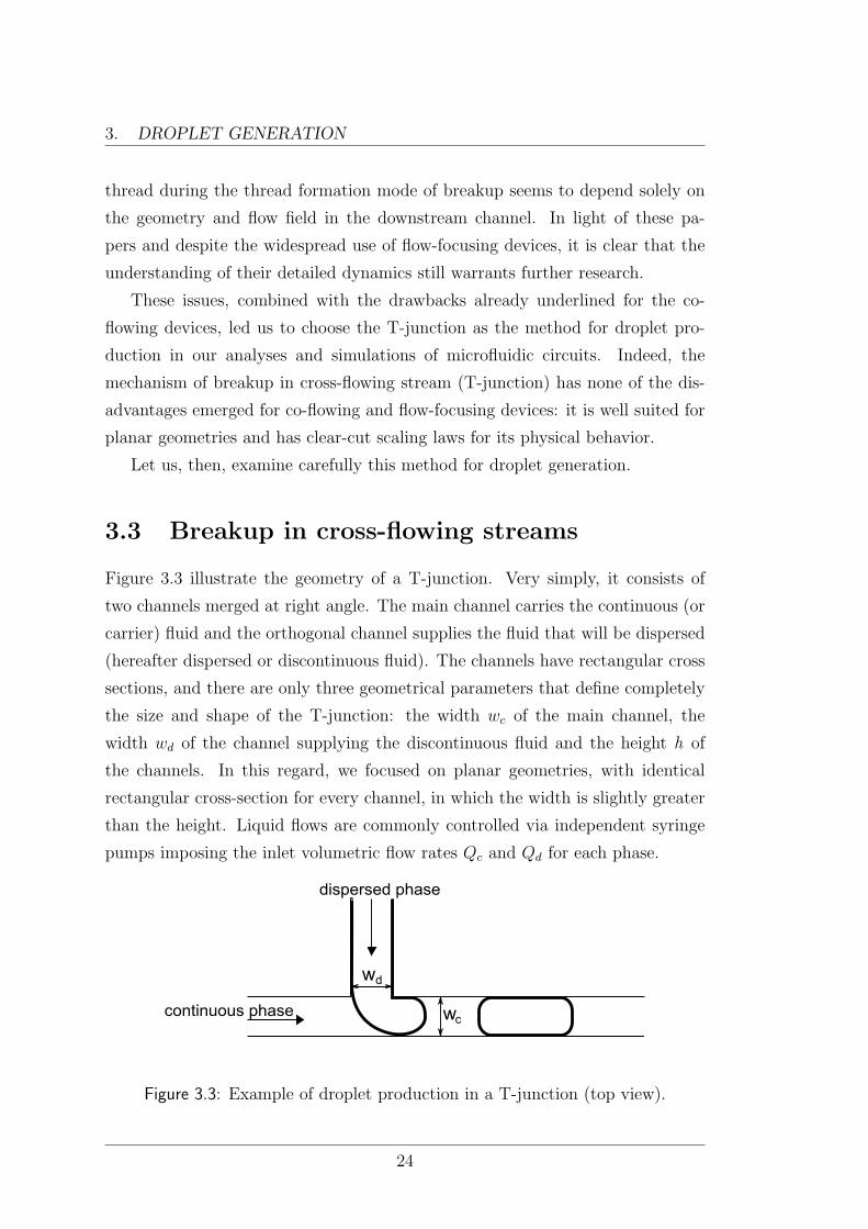
Figure 3.3 illustrate the geometry of a T-junction. Very simply, it consists of
two channels merged at right angle. The main channel carries the continuous (or
carrier) fluid and the orthogonal channel supplies the fluid that will be dispersed
(hereafter dispersed or discontinuous fluid). The channels have rectangular cross
sections, and there are only three geometrical parameters that define completely
the size and shape of the T-junction: the width wc of the main channel, the
width wd of the channel supplying the discontinuous fluid and the height h of
the channels. In this regard, we focused on planar geometries, with identical
rectangular cross-section for every channel, in which the width is slightly greater
than the height. Liquid flows are commonly controlled via independent syringe
pumps imposing the inlet volumetric flow rates Qc and Qd for each phase.
dispersed phase
continuous phase
wd
wc
Figure 3.3: Example of droplet production in a T-junction (top view).
24

3.3 BREAKUP IN CROSS-FLOWING STREAMS
3.3.1 Forces anlysis
The process of droplet formation actually begins as soon as the dispersed phase
starts penetrating into the outer channel. Here, three main forces act on the
emerging interface and influence droplet breakup: the viscous shear-stress force
(Fτ ), the surface (or interfacial) tension force (Fσ) and the force arising from
the increased resistance to flow of the continuous fluid around the tip (hereafter
“squeezing force”, FS). The understanding of their balance is crucial for draw-
ing the correct model of the breakup process so, in the next paragraphs, we
will examine, one by one, the contribution given by these forces during droplet
generation.
Viscous shear-stress force A viscous shear stress is defined as the component
of stress co-planar with a material cross section. In our case, this kind of stress
is exerted on the dispersed phase by the cross-flow of the continuous phase. Its
magnitude is estimated by the product µcG, where µc is the viscosity of the carrier
fluid and G is a characteristic rate of shear strain that is proportional to Qc and is
a function of the T-junction and the emerging interface geometry. More in detail,
we can approximate this stress as τ = µcugap/ϵ, where ugap = Qc/(hϵ) is the
speed of the continuous fluid flowing through the gap, of characteristic thickness
ϵ, between the interface and the wall of the channel (see Figure 3.4). In order to
estimate the net force acting on the immiscible tip, we then multiply the shear
stress τ = µcQc/(hϵ2) by the surface area of the interface in the gap Agap ∼ hw1,
where we take w as the characteristic axial length-scale of the tip (see Figure 3.4).
Finally, the corresponding net force on the tip is pointed downstream and has
the magnitude of:
Fτ ≈ µcQcw
ϵ2. (3.1)
Squeezing force The so called squeezing force comes into play when the thread
of the discontinuous fluid almost obstructs the cross section of the main channel
(see Figure 3.4). In this situation, the available area through which continuous
fluid can pass is significantly restricted leading to an increased pressure directly
upstream of the junction. As detailed below, the magnitude of the squeezing
1The shear stress, in fact, is given by the ratio between the force applied and the surface
affected by the stress τ = Fτ
A .
25

3. DROPLET GENERATION
ε
ratip
raup
~w
dispersed phase
continuous phase
Figure 3.4: Schematic illustration (top view) of the shape of the immiscible
thread’s tip at an intermediate stage of break-up in a T-junction.
pressure increases dramatically as the distance between the emerging interface
and the opposing wall of the main microchannel (ϵ) decreases. For ϵ ∼ w, using
the Hagen-Poiseuille’s law referred to a rectangular channel (see Section §2.5),
we can estimate the pressure drop ∆p over the length (∼ w) of the immiscible
tip: ∆p ≈ µcQcw/(h2ϵ2). When ϵ ≪ w, instead, we evaluate ∆p for a thin film of
typical thickness ϵ, width h and length w (Figure 3.4): ∆p ≈ µcQcw/(hϵ3), and
the corresponding net force obtained, oriented downstream, is equal to:
FS ≈ ∆phw = µcQcw2
ϵ3. (3.2)
The exact value of the exponent n to which the thickness of the film ϵ should
be raised in the above expression can be derived from a detailed lubrication
analysis[6] for flow around objects near-filling the cross-sections of capillaries: n
depends on the geometry of the cross-section of the capillary and on the geom-
etry and material parameters of the object. Importantly, n is larger than 2 and
consequently we can expect that FS > Fτ when ϵ ≪ w.
Interfacial tension force Surface tension is a contractile tendency of the sur-
face of a liquid that allows it to resist an external force. The cohesive forces
among liquid molecules are responsible for the phenomenon of surface tension.
Very simply, it can be interpreted as follows: in the bulk of the liquid, each
molecule is pulled equally in every direction by neighboring molecules, resulting
in a net force of zero. The molecules at the surface, differently, are not surrounded
by similar molecules on all sides and therefore are pulled inwards.
26

3.3 BREAKUP IN CROSS-FLOWING STREAMS
In our case, in particular, the surface tension is ruled by the interaction
between dissimilar liquid (dispersed and continuous phase). This kind of sur-
face tension is called interfacial tension, but its physics are almost the same.
It resists deformation due to continuous fluid by establishing a pressure jump
across the curved edge of the growing droplet. In particular, the surface tension
force is associated with the Laplace pressure jump ∆pL across a static interface,
∆pL = σ(r−1a + r−1
r ) where σ is the interfacial tension coefficient (sometimes de-
noted γ), ra is the axial curvature (in the plane of the device) and rr is the radius
of the radial curvature (in the cross-section of the neck joining the inlet for the
discontinuous fluid with the tip). In the intermediate stage of the process of for-
mation of a droplet (Figure 3.4) the radial curvature is bounded by the height
of the channels (h < w) and rr ≈ h/2 (or less) everywhere. The axial curvature
is more emphasized at the downstream tip of the immiscible thread (rtipa ≈ w/2)
than at the upstream side of it (rupa ≈ w): the interface on the downstream side of
the thread acts on the liquid inside the thread with a stress pL ≈ −σ(2/w + 2/h)
(the minus sign signifies that the stress is oriented upstream), and the interface lo-
cated upstream acts on the discontinuous liquid with a stress pL ≈ σ(1/w + 2/h)
(oriented downstream). The sum of the two, multiplied by the cross-section of
the channel gives the following estimation of the interfacial tension force:
Fσ ≈ −σh, (3.3)
which has a stabilizing effect on the tip: in the absence of any other stresses or
forces, surface tension would position the tip symmetrically about the axis of the
inlet channel for the dispersed phase.
To summarize the order-of-magnitude estimates of the forces acting on the tip,
we note that the only stabilizing force arises from the interfacial tension effects
(see Equation (3.3)). On the other hand, there are two destabilizing forces (see
Equation (3.2) and (3.1)), both of which increase sharply upon the decrease of
the separation ϵ between the interface and the opposing wall of the main channel.
As stated by several studies[7, 8, 9], the balance of these forces leads to the
definition of two principal regimes of breakup in T-junction:
squeezing regime;
dripping regime.
27

3. DROPLET GENERATION
Importantly, the transition between them is governed by the Capillary number
(Ca) which is a dimensionless parameter that describes the relative magnitude of
the viscous shear stress compared with the interfacial tension (see Section §2.2).
A simple definition for Ca in microfluidics is given in terms of the average velocity
uc of the continuous phase, the dynamic viscosity µc of the continuous phase and
the interfacial tension coefficient σ:
Ca =µcuc
σ=
µcQc
σwh. (3.4)
In particular, for low values of the Capillary number (Ca < CaCR), ie when the
interfacial forces dominate the shear stress, the dynamics of breakup of immiscible
thread in T-junction is dominated by the squeezing force across the droplet as
it forms (squeezing regime). In the opposite case (Ca > CaCR), the shear stress
starts playing an important role and the system starts operating in the so called
dripping regime. As reported in recent papers[8] and confirmed in our numerical
simulations, this threshold is given by:
CaCR ≈ 10−2. (3.5)
Let us now examine in more detail the two regimes mentioned above with a
particular focus on the squeezing regime which is the one we will adopt later on for
our microfluidic networks because it shows the best flexibility and controllability
over the shape of the droplets generated.
3.3.2 Squeezing regime
The typical process of droplets formation via squeezing regime is visually de-
picted in the simulation of Figure 3.5 where the principal geometrical and phys-
ical parameters imposed are the following: h = 50µm,wc = wd = 150µm,Qc =
3.75nL/s,Qd = 1.875nL/s. Keeping it in mind and on the basis of the previous
analysis and observations, the mechnism in question can be briefly described as
follows: the two immiscible fluids form an interface at the junction of the dis-
persed inlet channel with the main channel. The stream of the discontinuous
phase starts penetrating into the main channel and a droplet begins to grow
under the effect of the viscous shear-stress force (Figure 3.5(a)). The latter, how-
ever, is not sufficient to distort the interface significantly because this operating
regime works under the condition Ca < CaCR ⇒ interfacial tension dominates
28

3.3 BREAKUP IN CROSS-FLOWING STREAMS
shear stress. Consequently, the emerging droplet manages to fill the junction and
restricts the available area through which continuous fluid can pass, leading to an
increased pressure directly upstream of the junction (Figure 3.5(b)). When the
corresponding squeezing force overcomes the interfacial tension force, the neck of
the emerging droplet squeezes (Figure 3.5(c)), promoting its breakup. Finally,
the disconnected liquid plug flows downstream of the main channel, while the tip
of the dispersed phase retracts to the end of the inlet and the process repeats
(Figure 3.5(d)). The intrinsic high reproducibility shown by this mechanism is
fundamental for the stable production of uniform droplets with identical length
and shape (Figure 3.5(e)) over a wide range of flow rates. This is also the reason
why we chose to work under squeezing regime in our simulations of T-shaped
droplet inlet systems.
(a) (b)
(c) (d)
(e)
Figure 3.5: Typical process of droplet formation in squeezing regime.
29

3. DROPLET GENERATION
Droplets length Applying the model of evolution of breakup at the T-junction
in the squeezing regime presented so far, Garstecki et al.[8] obtain a simple for-
mula for the length Ld of the resulting droplets:
Ld = w(1 + αQd
Qc) (3.6)
where w is the width of the main channel, Qd is the flow of the dispersed phase,
Qc is the flow of the carrier fluid and α is a dimensionless parameter of order
one. Equation (3.6) can be intuitively understood by arguing that detachment
begins once the emerging discontinuous thread fills totally the main channel,
i.e. when the squeezing force is stronger. At this moment, the length of the
droplet is approximately equal to the width of the channel w and the thickness of
the neck in the junction starts decreasing at a rate which depends on the mean
speed of the continuous fluid uc. So, the flow of the carrier fluid (Qc = uchw)
sets the time for the growth of the droplet because it determines the “squeezing
time” necessary for the neck to break. This results in an inverse proportionality
between droplet length and continuous phase flow (Ld ∝ 1Qc). In fact, considering
an equal input discontinuous phase flow, the greater the continuous flow the lower
the squeezing time and thus the length of the resulting droplets. On the other
hand, there is a direct proportionality between droplet length and dispersed phase
flow (Ld ∝ Qd) because Qd determines how much discontinuous fluid manages to
flow in the droplet before the squeezing time imposed by the flow of the carrier
fluid ends and breakup occurs.
Interdistance between droplets Another physical parameter to be consid-
ered, that’ll be useful later on, concerns the spacing δ[m] between droplets gener-
ated in squeezing regime. Its scaling relation can be deduced, as reported below,
thanks to the application of the mass conservation law.
Let us consider a sufficiently long time τ and the related distance x = u′dτ
along the main channel (being u′d the velocity of the dispersed fluid in the main
channel). The number of droplets along x in the time interval τ is given by:
nd(τ) =x
Ld + δ=
u′dτ
Ld + δ, (3.7)
where Ld is the length of the single droplet and δ is the interdistance between
them (see Figure 3.6).
30

3.3 BREAKUP IN CROSS-FLOWING STREAMS
dispersed phase
continuous phase
Ld Ld Ldδ δ
Figure 3.6: Schematic illustration of a train of droplets created by a T-junction.
Now, the mass conservation law imposes that the volume of dispersed liquid
injected by the discontinuous phase inlet channel throughout the time interval τ
(V old,in = Qdτ = udwhτ) corresponds to the volume of dispersed fluid along x in
the main channel (V old,x = Ldropletwhnd = Ldwhu′dτ
Ld+δ):
udwhτ = Ldwhu′dτ
Ld + δ⇒ ud(Ld + δ) = Ldu
′d. (3.8)
The next step requires the evaluation of the velocity of the dispersed fluid in the
main channel u′d. To determine it, we make the hypothesis that dispersed and
continuous phase flow at the same velocity (u′d = u′
c = u) in the main channel,
though it is not always true[10]. Then, we can exploit the parallelism that exist
between the microfluidic and electrical circuit (see Section §2.7) as reported in
Figure 3.7: in particular, we can associate the flow of the fluids (Qd, Qc, Q) in the
microchannels of the T-junction to the current in the analogous electrical circuit
(Id, Ic, I). In this way, by applying Kirchhoff’s law we obtain I = Id + Ic and
thus:
Q = Qd +Qc ⇒ u = ud + uc.2 (3.9)
Substituting Equation (3.9) in (3.8), it results:
ud(Ld + δ) = Ld(ud + uc) ⇒ δ = Lduc
ud
= LdQc
Qd
. (3.10)
Finally, replacing (3.6) in (3.10), we obtain the desired formula for the interdis-
tance between droplets generated in a T-junction in the squeezing regime:
δ =Qc
Qd
w(1 + αQd
Qc). (3.11)
2The last implication follows from the fact that we always consider channels with identical
cross section.
31

3. DROPLET GENERATION
Qd
Qc Q
Ic
Id
I
ri
ri
R
Figure 3.7: Analogy between microfluidic T-junction and electric circuit.
Lingering on Equation (3.10), it can be noted that droplets length and inter-
distance are strictly correlated since δ depends on Ld. Consequently, once fixed
the geometry of the system and the physical parameters of the liquids, bubbles
with a specific length will have a corresponding precise interdistance between
them. In order to decorrelate the two values and make δ independent of Ld the
solution proposed by Jullien et al.[11] can be adopted. Basically, it consists in
arranging, downstream of the T-shaped droplet generator, a series of small entries
forming a comb (see Figure 3.8) which injects additional continuous phase, sepa-
rating the droplets by variable lengths, typically several hundred of micrometers.
On the contrary, if we want to near the bubbles, the comb can be employed to
eject part of the continuous fluid between the droplets. In this way, we are able
to modulate droplet interdistance irrespective of their length.
dispersed phase
continuous phase
continuous phase
Figure 3.8: Sketch of droplet generator and comb to modulate droplet interdis-
tance.
Simulations and numerical results In order to validate the theoretical anal-
ysis presented so far, we made use of the cfd software OpenFOAM (see Appendix
A) to implement a T-junction device for droplet generation. The microchannels
geometries imposed in our simulations are listed in Table 3.1 while in Table 3.2
32

3.3 BREAKUP IN CROSS-FLOWING STREAMS
are reported the common physical properties of the fluids considered.
System geometry
Channels’ height h 50 µm
Main channel’s width wc 150 µm
Dispersed channel’s width wd 150 µm
Table 3.1: Geometrical properties of the reference system
Fluids’ properties
Continuous phase→water
Dynamic viscosity µc 1.002 mPa · sDensity ρc 1000 Kg/m3
Kinematic viscosity νc 1.002 mm2/s
Dispersed phase→silicone oil
Dynamic viscosity µd 145.5 mPa · sDensity ρd 970 Kg/m3
Kinematic viscosity νd 150 mm2/s
Interfacial tension coefficient σ 46 mN/m
Table 3.2: Physical properties of the fluids considered
For this reference system, we plot the droplet length and interdistance as
a function of the flow rate ratio φ = Qd/Qc obtained in our simulations. In
particular, we selected three different fixed inlet velocities for the continuous
phase, namely uc = k · uc,st [m/s] such that Qc = k · whuc,st [m3/s] with uc,st =
0.0005 m/s and k = 0.5, 1, 2 and collected the relative results in Figure 3.9,
3.10 and 3.11 respectively. For each fixed continuous flow, the quantity φ =
Qd/Qc is varied in the range from 0.25 to 6.5 by opportunely incrementing the
dispersed phase inlet flow Qd. The simulative data (denoted by markers in the
graphs) agrees very well, both for droplet length and droplet interdistance, with
the theoretical model (continuous lines in the figures) expressed in Equations
(3.6) and (3.11).
In addition, in Figure 3.12 we reported all together the graphs obtained for the
three cases under examination. Analyzing the latter, it transpires the dependence
of the fitting parameter α of Equation (3.6) from the absolute velocity set for
the continuous phase. The various slopes obtained for the theoretical curves, in
fact, denote different values of the prameter α: in particular, an increase in uc
corresponds to a decrease in α.
33

3. DROPLET GENERATION
0 1 2 3 4 5 6 70
0.5
1
1.5x 10
−3
Qd/Q
c
L d [m]
droplet length for uc=0.5mm/s
(a)
0 1 2 3 4 5 6 70
0.1
0.2
0.3
0.4
0.5
0.6
0.7
0.8
0.9
1x 10
−3
Qd/Q
cδ
[m]
droplet interdistance for uc=0.5mm/s
(b)
Figure 3.9: (a) Length and (b) spacing between droplets produced in a T-junction
for a fixed value of uc = 0.5mm/s ⇒ Qc = 3.75nL/s. Continuous lines represents
the theoretical curves obtained from (a) Eq. (3.6) and (b) Eq. (3.11) with α = 1.3.
Markers corresponds to the simulative results obtained with OpenFOAM.
0 1 2 3 4 5 6 70
0.5
1
1.5x 10
−3
Qd/Q
c
L d [m]
droplet length for uc=0.25mm/s
(a)
0 1 2 3 4 5 6 70
0.1
0.2
0.3
0.4
0.5
0.6
0.7
0.8
0.9
1x 10
−3
Qd/Q
c
δ [m
]
droplet interdistance for uc=0.25mm/s
(b)
Figure 3.10: (a) Length and (b) spacing between droplets produced in a T-junction
for a fixed value of uc = 0.25mm/s ⇒ Qc = 1.875nL/s. Continuous lines rep-
resents the theoretical curves obtained from (a) Eq. (3.6) and (b) Eq. (3.11)
with α = 1.5. Markers corresponds to the simulative results obtained with Open-
FOAM.
34

3.3 BREAKUP IN CROSS-FLOWING STREAMS
0 1 2 3 4 5 6 70
0.5
1
1.5x 10
−3
Qd/Q
c
L d [m]
droplet length for uc=1mm/s
(a)
0 1 2 3 4 5 6 70
0.1
0.2
0.3
0.4
0.5
0.6
0.7
0.8
0.9
1x 10
−3
Qd/Q
c
δ [m
]
droplet interdistance for uc=1mm/s
(b)
Figure 3.11: (a) Length and (b) spacing between droplets produced in a T-junction
for a fixed value of uc = 1mm/s ⇒ Qc = 7.5nL/s. Continuous line represents the
theoretical curves obtained from (a) Eq. (3.6) and (b) Eq. (3.11) with α = 1.1.
Markers corresponds to the simulative results obtained with OpenFOAM.
0 1 2 3 4 5 6 70
0.5
1
1.5x 10
−3
Qd/Q
c
L d [m]
droplet length
theoretical Ld with u
c=0.5mm/s
simulative Ld with u
c=0.5mm/s
theoretical Ld with u
c=0.25mm/s
simulative Ld with u
c=0.25mm/s
theoretical Ld with u
c=1mm/s
simulative Ld with u
c=1mm/s
(a)
0 1 2 3 4 5 6 70
0.1
0.2
0.3
0.4
0.5
0.6
0.7
0.8
0.9
1x 10
−3
Qd/Q
c
δ [m
]
droplet interdistance
theoretical δ with uc=0.5mm/s
simulative δ with uc=0.5mm/s
theoretical δ with uc=0.25mm/s
simulative δ with uc=0.25mm/s
theoretical δ with uc=1mm/s
simulative δ with uc=1mm/s
(b)
Figure 3.12: Collection and comparison of the data (a) from Figure 3.9(a), 3.10(a),
3.11(a) and (b) from Figure 3.9(b), 3.10(b), 3.11(b).
35

3. DROPLET GENERATION
Finally, we noted that for low values of φ = Qd/Qc the numerical results
follows almost ideally our model while non linearity and anomalous behaviors
emerge as soon as φ is increased too much. Indeed, when Qd > 7Qc the squeez-
ing regime further evolves in a sort of “parallel flow” regime, visually repre-
sented in the simulation of Figure 3.13 where the parameters considered are
h = 50µm,wc = wd = 150µm,Qc = 3.75nL/s,Qd = 37.5nL/s. Remember-
ing Equations (3.6) and (3.11), this simulative evidence, translates in an upper
bound for the droplet length and in a lower bound for the droplet interdistance
achievable once imposed the reference geometry.
Figure 3.13: Degeneration of squeezing regime for high values of φ = Qd/Qc.
3.3.3 Dripping regime
As already stated, the dripping regime occurs when we work under the condition
CaCR > 10−2. In this case, contrary to the squeezing regime, droplet formation
is entirely due to the action of the shear stress which is large enough to overcome
the interfacial tension, analogous to spherical droplet breakup.
The typical mechanism of bubble production under dripping regime is illus-
trated step by step in the simulation reported in Figure 3.14 (the reference system
considered here has got h = 50µm,wc = wd = 150µm, the continuous phase is
characterized by µc = 145.5 mPa · s and Qc = 7.5nL/s while for the dispersed
phase we imposed µc = 1.002 mPa · s and Qd = 7.125nL/s). As soon as the
dispersed phase enters the main channel (Figure 3.14(a)), it is affected by the
36

3.3 BREAKUP IN CROSS-FLOWING STREAMS
strong viscous shear-stress force Fτ caused by the carrier fluid. Accordingly,
the emerging interface is sensitively distorted (Figure 3.14(b))and droplets are
emitted before they can block the main channel (Figure 3.14(c)). This physical
behavior, however, involves a strong limitation on the production of droplet which
will consequently always be shorter than the width of the main channel w. For
the same reason, the frequency of production of droplets is much higher than the
corresponding one in the squeezing regime. This closeness between droplets can,
in the worst case, entail the fusion of the same in the outer channel.
(a) (b)
(c)
Figure 3.14: Typical process of droplet formation in dripping regime.
Scaling models[2] developed to describe this process also demonstrate that the
droplet size depends predominantly on the capillary number Ca and not on the
flow rate ratio φ: de facto, it decreases strongly as the capillary number increases.
Furthermore, larger viscosity ratios λ = µd
µclead to smaller droplets.
As long as the inlet velocities imposed for the continuous and dispersed phase
are quite low (uc, ud < 10−2), our simulations agrees well with the theoretical
background presented (see Figure 3.14 for a practical example). At greater orders
of magnitude, instead, we observed that the dripping regime evolves into the
formation of stable parallel flowing streams, as reported in Figure 3.15 for a
reference system with h = 50µm,wc = wd = 150µm,Qc = 97.5nL/s,Qd =
71.25nL/s. We conjecture that the origin of this phenomenon lies in the fact
37

3. DROPLET GENERATION
that, for the reference velocities, the frequency of droplet production is so high
that it degenerates in a continuous stream.
Figure 3.15: Degeneration of dripping regime for high values of ud and uc.
38

Chapter 4
Characterization of droplet
dynamics in a bifurcating channel
After analyzing in detail the process of droplets generation, the next topic to be
addressed, in order to understand the complex dynamics at the basis of microflu-
idic systems, concerns the behavior of droplets once they meet a bifurcation along
the network.
Our interest in understanding the physics governing droplet dynamics in bi-
furcating channels, stem from the fact that we wish to convey droplets to the
microfluidic machines. The latters are, in fact, physically connected to the net-
work by means of ramifications.
On this purpose, we’ll divide the present chapter in two main section: in the
former one we are going to outline the so called droplet’s breaking/non-breaking
regions while in the latter we are going to point out how to passively pilot the
droplets in a specific target arm of the bifurcation.
4.1 Droplet breakup in a bifurcating channel
If we consider the droplets, in analogy with the world of telecommunications, as
the “packets” we want to deliver to the “end users” (microfluidic machines) of
our network, we need to preserve their integrity throughout the entire system
and, thus, even when they pass through “sensitive points” such as bifurcating
channel.
Several studies, numerical simulations and experimental evidencies[12, 13, 14]
39

4. CHARACTERIZATION OF DROPLET DYNAMICS IN ABIFURCATING CHANNEL
have been published in literature on this subject. Most of the studies focus on the
T-junctions, where a channel splits into two symmetric arms, forming a T. In such
systems, as we are going to formalize, depending on droplet size, capillary number
and viscosity ratio of the dispersed and continuous phase, droplets arriving at the
junction may either split or flow completely along one of the arm of the T.
Hereafter, we’ll seek in particular to define the parameter range that controls
the transition between breaking and non-breaking regime. Proceeding with order,
we now describe the physics behind breakup and non-breakup regimes.
4.1.1 Breakup regime
Figure 4.1 describes the temporal droplet evolution obtained from a simulation
characterized by the reference geometrical and physical parameters listed in Ta-
bles 3.1 and 3.2 and an inlet velocity of uc = 0.00075m/s.
(a) (b)
(c) (d)
Figure 4.1: Typical droplet dynamics in breakup regime at the bifurcation.
Figure 4.1(a) shows the elongated droplet as it is just about to come in contact
with the edge of the junction. Immediately, it deforms symmetrically forming two
identical liquid fingers in the upper and lower branch, which almost completely
fill the channel (see Figure 4.1(b)). Then, the droplet rear forms a curvature
at the entrance of the bifurcation bulging in the upstream direction. In this
40

4.1 DROPLET BREAKUP IN A BIFURCATING CHANNEL
process a neck forms in the central part of the junction with a width decreasing
in time (see Figure 4.1(c)). This behavior is presumably due to the flow of the
carrier phase which actually flattens the dispersed phase against the sidewall of
the bifurcation. As the circumference of the thread becomes less than its normal
length, the surface tension starts to contract it radially promoting the incipience
and growth of an instability similar to the Rayleigh-Plateau (see Section §2.6).
This eventually results in a pinch-off and the formation of two almost equally
sized daughter droplets that propagate downstream in the channel branches (see
Figure 4.1(d)).
4.1.2 Non-breakup regime
By reducing the Ca number, in comparison with the preceeding case, cohesion
forces become more relevant (see section 2.2), and thus we observe a radically
different droplet behavior as reported in Figure 4.2 for a system with halved
velocity uc compared to the previous one. Here, initially, the droplet reduces
its speed and approaches the junction in a similar fashion as reported above
(see Figure 4.2(a)). However, now, the dominating surface tension force reduces
the ability of the inertia and viscous force to deform the droplet which obtains
a quasi steady-state condition, with no internal flow, as it sticks in the junc-
tion. Due to the stronger interfacial force, a larger curvature is generated at the
droplet rear, resulting in a larger radius of the liquid thread (see Figure 4.2(b)).
This has a direct consequence on the resulting droplet dynamics, as the birth of
a Rayleigh-Plateau instability is prevented. The incipience of a random distur-
bance, generates a slightly asymmetric flow in the film formed between the droplet
interface and the channel surface opening a tunnel on one side of the junction
(see Figure 4.2(c)). As this perturbation grows, the droplet starts steering in the
opposite arm (see Figure 4.2(d)) and eventually migrates entirely in this direction
(see Figure 4.2(e)). This leaves an asymmetric distribution of the phases in the
daughter branches and the droplet wrapping generates a continuous phase’s flow
recirculation in the other arm.
A mathematical formalization of the physical phenomena involved in breakup
and non-breakup regimes has been proposed in a recent paper by Leshansky
and Pismen[14]. Indeed, they developed an analytical theory that describes the
41

4. CHARACTERIZATION OF DROPLET DYNAMICS IN ABIFURCATING CHANNEL
(a) (b)
(c) (d)
(e)
Figure 4.2: Typical droplet dynamics in non-breakup regime at the bifurcation.
42

4.1 DROPLET BREAKUP IN A BIFURCATING CHANNEL
breakup process in a symmetric two-dimensional T-junction driven by the obser-
vation of the pressure evolution in the droplet at the bifurcation. Although this
analysis works in a limited 2D setting, the formula derived by Leshansky and
Pismen agrees well with both 2D and 3D simulations and experimental findings
from literature[15].
In particular, they could determine the conditions under which stationary
solutions exist. This range corresponds, physically, to non-breakup case that is,
as already stated, the case we are interested in. On this purpose, the boundary
between non-breakup and breakup regions is given by the following important
formula (continuous line in Figure 4.3):
Ld
w≈ χCa−0.21 (4.1)
where Ld [m] is the length of the droplet that approaches the T-junction, w [m]
is the width of the channels, Ca is the Capillary number (see Section §2.2) and
χ is a dimensionless parameter that depends on the ratio between the viscosities
of dispersed and continuous phase λ = µd
µc: experimental evidences[11] demon-
strate that the fitting χ decreases as λ increases. It can be noted that, once we
fix λ, the transition between non-breakup and breakup regions is ruled only by
two parameters: Ca and Ld (w is, in fact, a fixed geometrical parameter of the
microfluidic system). In details, if we consider Ld as a constant, lower Capillary
numbers lead to a wider non-breakup region. This behavior can be intuitively
explained by ascertaining that small Capillary numbers mean that interfacial ten-
sion force dominates viscous force and thus it correspond to a situation of big
cohesion between droplet’s molecules.
On the other side, if we fix Ca, the greater is the droplet’s length, the lower the
corresponding non-breakup region. In turn, this phenomenon finds the following
intuitive explanation: the least energy configuration for a droplet corresponds to
the spherical geometry. Now, since physical systems tend intrinsically to move
to the minimum energy state, breakup will affect more easily the most elongated
drops (which are also the most energetic ones) in order to take them back to a
spherical shape.
43

4. CHARACTERIZATION OF DROPLET DYNAMICS IN ABIFURCATING CHANNEL
4.1.3 Simulations and numerical results
In order to validate the theoretical background presented, we carried out a se-
ries of simulations in symmetric 3D T-junctions using the finite volume based
open-source code OpenFOAM (see Appendix A). The breakup has been simu-
lated in a confined T-junction with uniform channels’ width w = 150µm and
height h = 50µm at varying Capillary numbers Ca = µcuc
σand different initial
length Ld of the parent droplet. Our simulations almost successfully capture the
transition between breaking and non-breaking regimes. It is shown (Figure 4.3)
that if Capillary number is smaller than a critical number given by Equation
(4.1), the droplet will move either to the left or right instead of breaking into
two daughter droplets. Moreover, the critical Capillary number decreases with
increasing droplet length. The χ parameter of Equation (4.1) considered in the
theoretical curve of Figure 4.3 is equal to 0.187.
1 1.5 2 2.5 3
0.2
0.4
0.6
0.8
1
1.2
1.4
1.6
1.8
2x 10
−4
Ld/w
Ca
theoretical boundbreakupnon−breakup
Figure 4.3: Phase diagram of numerical simulations for a drop in a symmetric
T-junction. The solid line is the theoretical curve given by Equation (4.1) for
χ = 0.187. The symbols correspond to numerical results for nonbreaking () andbreaking () drops.
44

4.2 REGULATION OF DROPLET TRAFFIC IN A T-JUNCTION
4.2 Regulation of droplet traffic in a T-junction
The next logical step we need to deal with, is the definition of a method to
precisely carry the non-splitting droplets in the desired arm of the T-junction.
The solution to this problem is provided by a simple property of microfluidic
droplet systems[16, 17] at a T-junction (neglecting splitting, direct interactions
and collisions) an arriving droplet follows the instantaneously leading flow rate.
So, if the total original flow rate Q of the parent channel divides between Q1 and
Q2 = Q−Q1 in the two daughter branches (see Figure 4.4(a)), the sign of Q1−Q2
decides in which arm the arriving droplet goes. More precisely, if Q1 > Q2 the
choice falls on the daughter channel number 1 and vice versa.
Accordingly, if we manage to create an asymmetry in the flows of the two
arms of a bifurcation, we are able to predict exactly the direction of the coming
droplets. In order to do this, let’s start noting that the T-junction depicted
in Figure 4.4(a) corresponds, thanks to the electric circuit analogy (see Section
§2.7), to the parallel resistance reported in Figure 4.4(b).
Q
Q1
Q2
L1
L2
(a)
Q1
Q2
Q
RH,2
RH,1
(b)
Figure 4.4: (a) Microfluidic symmetric T-junction and (b) its analogous electric
circuit.
Moreover, we remember the concept of hydraulic resistance of a generical
microfluidic channel introduced in Section §2.7, which is given by:
RH,i =aµcLi
wh3(4.2)
45

4. CHARACTERIZATION OF DROPLET DYNAMICS IN ABIFURCATING CHANNEL
where µc[Pa · s] is the dynamic viscosity of the flowing liquid, Li[m] is the length
of the channel, w[m] is the width of the channel, h[m] is the height of the channel
and a is a dimensionless parameter defined as a = 12[1− 192hπ5w
tanh(πw2h)]−1.
Premising that w, h and consequently a are normally identical for the two
arms of a T-junction, we can opportunely change L1 and L21 (see Figure 4.5(a))
in order to obtain RH,1 = RH,2. In particular, L1 > L2 ⇒ RH,1 > RH,2. In this
way, we are able to achieve the desired initial unbalance between Q1 and Q2 that
can be calculated using the current division law (see Section §2.7):
Q1 =RH,2
RH,1 +RH,2
Q Q2 =RH,1
RH,1 +RH,2
Q (4.3)
Therefore, relying on the previous equation, the arm with the leading flow
rate Qi in the bifurcation is the one with lower hydraulic resistance RH,i (channel
1 in figure Figure 4.5(a)) and the choice of the incoming non-splitting droplet will
fall on this one (see Figure 4.5(b)).
The last aspect left to evaluate concerns the analysis of the effects induced by
the presence of a droplet in one arm of the bifurcation. As we already pointed
out in the non-breaking regime description, flows involving non-splitting droplets
are inherently asymmetric since the presence of the latter in one arm of the T-
junction increases the volumetric flow rate of the opposite channel. In this way,
droplets act as a series flow resistance in the branch they occupy.
In order to quantify the additional resistance involved by droplets, we should
notice that their presence in a channel change the dynamic viscosity µd of the por-
tion Ld they occupy. Thus, referring to Equation (2.21), the hydraulic resistance
ascribable to the droplet is given by:
RH,d =µdLda
wh3(4.4)
Then, the new resistance (R′H,i) of the channel, can be obtained by summing
RH,d to the original hydraulic resistance (RH,i) of the same and subtracting the
quantity µcLdawh3 (this is due to the fact that the original RH,i considered a channel
completely filled by continuous phase which is not true anymore for the portion
1For the moment, we exclude the presence of any droplets in the bifurcation, so µ1 = µ2 = µc,
because we are interested in the behavior of the first drop that approach the T-junction. The
opposite case is discussed later.
46

4.2 REGULATION OF DROPLET TRAFFIC IN A T-JUNCTION
Ld occupied by the droplet). So, we can rewrite R′H,i as follows:
R′
H,i = RH,i + δr =aµcLi
wh3+ (µd − µc)
Lda
wh3(4.5)
where δr = (µd − µc)Ldawh3 is the additional resistance per droplet.
Accordingly, in the case of Figure 4.5(b), the current division law returns:
Q′
1 =RH,2
RH,1 + δr +RH,2
Q Q′
2 =RH,1 + δr
RH,1 + δr +RH,2
Q (4.6)
Finally, two different cases may occur:
if Q′1 is still greater than Q
′2 in Figure 4.5(b), the next coming droplet will
select, in turn, channel number 1 in the bifurcation (see Figure 4.5(c));
if δr is great enough to invert the channel with the leading flow rate (Q′2 >
Q′1 in Figure 4.5(b)), the next coming droplet will select branch 2 differently
from the first bubble’s choice (see Figure 4.5(d)).
From this examination, we can appreciate how the droplet sorting problem is
intrinsically non linear and complex. The hydrodynamic resistance of each arm
of the bifurcation depends, in fact, both from its geometrical properties and from
the number and size of the droplets it contains. Consequently, the instantaneous
“choice” of the droplets depends on the past hystory of the flow. Such a nonlinear
“memory kernel” renders the process very sensitive and complicates significantly
its analysis.
4.2.1 Simulative example
In order to validate the model introduced for the droplet sorting problem, we ran
several simulations using OpenFOAM, experiencing an almost perfect agreement
with our theoretical solution.
On this purpose, Figure 4.6 represent a significant example. Here, we collect
the results obtained from a simulation characterized by the following settings:
We can observe, in accordance with the theory, that the first droplet approach-
ing the bifurcation (Figure 4.6(a)) turns to the right channel (lower channel in
Figure 4.6(b)): this branch, in fact, is shorter than the other one and has, conse-
quently, the lowest initial hydraulic resistance (see Equation (4.2)):
RH,1 =aµcL1
wh3 ≈ 1.62 · 1012Pa · s/m3
RH,2 =aµcL2
wh3 ≈ 4.05 · 1012Pa · s/m3(4.7)
47

4. CHARACTERIZATION OF DROPLET DYNAMICS IN ABIFURCATING CHANNEL
Q
Q1
Q2
L1
L2
(a)
Q
Q'1
Q'2
L1
L2
(b)
Q
Q"1
Q"2
L1
L2
(c)
Q
Q"1
Q"2
L1
L2
(d)
Figure 4.5: Example of droplet sorting problem.
48

4.2 REGULATION OF DROPLET TRAFFIC IN A T-JUNCTION
Simulation settings
Dispersed phase viscosity µd = 145.5 mPa · sContinuous phase viscosity µc = 1.002 mPa · sDroplets’ length Ld1 = Ld2 = 200 µm
Channels’ width w = 150 µm
Channels’ height h = 50 µm
First branch’s length L1 = 2mm
Second branch’s length L2 = 5mm
Input volumetric flow rate Q = 2.625nL/s
Table 4.1: Geometrical and physical properties of the reference system
and thus the leading flow rate (see Equation (4.3)):
Q1 =RH,2
RH,1+RH,2Q ≈ 1.88nL/s
Q2 =RH,1
RH,1+RH,2Q ≈ 0.75nL/s
(4.8)
Immediately, the presence of the droplet in the right arm, increases its resistance
in accordance with Equation (4.5):
R′H,1 = RH,1 + δr1 =
aµcL1
wh3 + (µd − µc)Ld1
a
wh3 ≈ 2.50 · 1013Pa · s/m3
R′H,2 = RH,2 =
aµcL2
wh3 ≈ 4.05 · 1012Pa · s/m3(4.9)
This additional resistance is great enough to make Q′2 > Q
′1:
Q′1 =
R′H,2
R′H,1+R
′H,2
Q ≈ 0.37nL/s
Q′2 =
R′H,1
R′H,1+R
′H,2
Q ≈ 2.26nL/s(4.10)
and, thus, the next coming droplet will move, contrary to the previous case, to
the left channel (upper channel in Figure 4.6(c)).
Our idea is to exploit this physical behavior to direct the droplets in our
microfluidic network as illustrated in the next chapter.
In conclusion, it is important to note that our theoretical model predicts an
increase in the hydraulic resistance of the channel caused by the presence of a
droplet if and only if µd > µc (in accordance with Equation (4.5)). This phe-
nomenon can be explained remembering that viscosity (see Section §2.1) describes
the fluid’s internal resistance to flow: the greater the viscosity, the greater its re-
sistance to flow and vice versa.
49

4. CHARACTERIZATION OF DROPLET DYNAMICS IN ABIFURCATING CHANNEL
(a) (b)
(c)
Figure 4.6: Simulation of droplet sorting problem.
So, if droplets have a characteristic dynamic viscosity µd > µc we, effectively,
inject in the microfluidic system a substance that opposes strongly to the motion
and ultimately increases the resistivity of the channel it occupies (the term δr in
Equation (4.5) is positive). Otherwise, if µd < µc, we inject a mobile liquid which
decreases the hydraulic resistance of the carrier channel (the term δr in Equation
(4.5) becomes negative).
This dynamic is consistent with the simulations we obtained with OpenFOAM
though some experiments from research groups prove that there is an increase
in channel resistance even if we inject a dispersed phase having µd < µc. On
this purpose, we suppose that the lack of the occurrance of this behavior in
our simulations is imputable to the limitations of the solver used (see Appendix
A). Most likely, in fact, it isn’t able to capture the friction’s sources different
from viscous force (e.g., the pressure exerted to the droplet by the thin films of
continuous phase that wrap the dispersed fluid).
Consequently, the model proposed may fail for situations in which viscous
forces are not the dominant friction contribution and thus it is mainly applicable
when µd ≫ µc.
50

Chapter 5
Design and performance of a
microfluidic bus network
As anticipated, our aim is to create a programmable LoC in which several ele-
ments (microfluidic machines), able to perform specific laboratory functions, are
deployed in a single “unit” and connected together to form a network. Accord-
ingly, it is possible to support different complex laboratory processes in the same
chip simultaneously, which has several advantages: cost of LoCs could be reduced,
their reusability could be increased and their effectiveness could be improved by
supporting higher flexibility and time saving.
A crucial step in this direction is the identification of an appropriate approach
to transmit “packets” (droplets) to the “end users” (microfluidic machines) of the
microfluidic network. In this chapter we’ll analyze a promising solution to this
problem and discuss the performance obtained for a microfluidic network with
bus topology.
5.1 Mechanism for droplet routing
First of all, let’s then consider a microfluidic bus network topology as depicted
in Figure 5.1, where N is the number of microfluidic machines (MM) connected.
Physically, it simply consists of a main “transmission channel” ramified several
times in order to reach all the microfluidic machines. Let’s note that, for the sake
of simplicity, we considered a uniform spacing (L) between the various branches.
In such configuration, a drop destined to the i-th MM is injected into the network
51

5. DESIGN AND PERFORMANCE OF A MICROFLUIDIC BUSNETWORK
through a generator (see Section §3.3) placed at the “input port” on the left, cross
the main channel until it’s finally diverted in the i-th target branch.
Q
MM # 1
MM # 2
MM # 3
MM # N
LLL
L1
L2
L3
LN
Figure 5.1: Design of a microfluidic network with bus topology.
Once again, in order to fully understand the mechanism we developed for
routing the drops, comes in handy the fluidic/electric parallelism (see Section
§2.7). Accordingly, in Figure 5.2 we reported the electric circuit that correspond
to the fluidic network depicted in Figure 5.1 where R is the hydraulic resistance
due to the linking stretches of length L, Rn is the characteristic resistance of the
n-th branch and Req,n is the equivalent resistance seen downstream of the n-th
branch in case of droplets’ absence. Another important premise, that will be
understood later on, is to impose the common main channel to be the path with
the starting leading flow.
RRR
R3 R2 R1RNQ
Req,2 Req,1Req,3Req,N
Figure 5.2: Electric circuit analogous to the microfluidic bus network.
Suppose, now, that we want to bring a droplet cargo with a certain volume at
the i-th MM. Our solution to fulfill this goal requires the injection of two very close
droplets in the system: a “header droplet” and a “payload droplet”. As already
52

5.2 BUS NETWORK DIMENSIONING
discussed, the first one (hereafter header droplet) will always follow the path
with the original leading flow, i.e. the main microchannel, due to the hypothesis
just made. Furthermore, it will increment, time after time, the resistance of the
duct it occupies in accordance with Equation (4.5). This physical behavior may
allow us to deflect the following droplet in the desired target branch. Let’s, in
fact, focus on the generic i-th bifurcation which is constituted by two parallel
arms with characteristic original hydraulic resistances respectively equal to Ri
and Req,i = R + Ri−1 ∥ Req,i−1 (see Figure 5.2). The presence of the header
droplet in the portion connecting ramification i and i − 1 will change Req,i as
follows:
R′
eq,i = R + δri +Ri−1 ∥ Req,i−1 (5.1)
where δri =(µd−µc)aLdi
wh3 is the resistance increment due to the header droplet1.
If δri is large enough to reverse the leading flow arm at the i-th bifurcation, the
second drop (hereafter payload droplet) won’t flow anymore in the main channel
but it will rather enter in the i-th branch reaching the desired target microfluidic
machine. The header droplet, in turn, continues along the main channel and
it’s eventually discarded from the system via the output port on the right (see
Figure 5.1): this droplet, in fact, doesn’t carry “useful fluid” but it rather serves
only to divert the actual payload droplet to the correct destination.
So far, we have given a qualitative description of the routing process we devel-
oped. Now, however, we have to mathematically formalize it in order to correctly
model the microfluidic network of Figure 5.1.
5.2 Bus network dimensioning
First of all, we have seen that the header droplet must always flow along the
whole main channel without being deflected at any ramifications. Only in this
way, in fact, it may opportunely affect the payload droplets’ route deviating them
in the correct branch. This requirement translates, ultimately, in the following
1Note that we implicitly impose that the header droplet is in the channel connecting ramifi-
cation i and i− 1 when the payload droplet approaches the i-th bifurcation because we assume
that they are injected very closely to each other.
53

5. DESIGN AND PERFORMANCE OF A MICROFLUIDIC BUSNETWORK
condition:
Rn > Req,n, ∀n = 1, ..., N (5.2)
where Rn is the characteristic hydraulic resistance of the n-th branch and Req,n is
the equivalent parallel resistance seen downstream of the n-th branch in case of
droplet’s absence. Equation (5.2) can be rewritten by observing that the circuit
configuration of Figure 5.2 has an intrinsic redundancy. Indeed, the following
recursive pattern can be identified:
Req,n = R +Rn−1 ∥ Req,n−1, ∀n = 1, ..., N (5.3)
with Req,1 = R (or equivalently Req,0 = 0). This logical step allows us to calculate
Req,n as a function of Req,n−1. Substituting it in Equation (5.2), in fact, we obtain:
Rn > R +Rn−1 ∥ Req,n−1, ∀n = 1, ..., N (5.4)
This condition imposes, therefore, a lower bound to the various Rn which, con-
sequently, can be calculated as follows:
Rn = αReq,n = α(R +Rn−1 ∥ Req,n−1), ∀n = 1, ..., N (5.5)
with α being a dimensionless discretionary parameter strictly greater than 1
(α > 1).
Now, we need to establish the correct resistance increment δri caused by a
header droplet in order to deflect the cargo in a generic i-th branch of the network.
Thus, we have to impose two different conditions:
1. The payload droplet must select the branch containing the i-th microfluidic
machine when it arrives at the corresponding bifurcation. Mathematically,
it consists in having R′eq,i = R + δri + Ri−1 ∥ Req,i−1 > Ri, where R
′eq,i is
the equivalent resistance seen downstream of the i-th branch in case of i-th
header droplet’s presence. Consequently, δri > Ri−Req,i = Ri−(R+Ri−1 ∥Req,i−1).
2. Moreover, we must ensure that the payload droplet doesn’t enter into any of
the outreaches it encounters before the i-th bifurcation, which means that:
R′
eq,k = R+ δri +Rk−1 ∥ Req,k−1 < Rk, ∀k = i+ 1, ..., N . It can be demon-
strated that condition necessary and sufficient to satisfy this requirement
54

5.2 BUS NETWORK DIMENSIONING
is: R′eq,i+1 = R+ δri +Ri ∥ Req,i < Ri+1. Therefore, δri < Ri+1 −Req,i+1 =
Ri+1 − (R +Ri ∥ Req,i)
Generalizing the previous reasoning, we obtain both a lower and an upper bound
for the various δrn, ∀n = 1, ..., N (i.e. the resistance increments that a header
must entail in order to route the following payload droplet to the various n-th
microfluidic machine of the bus network). In particular, condition number 1.
implies:
δrn > Rn −Req,n, ∀n = 1, ..., N (5.6)
whereas, condition number 2. entails:
δrn < Rn+1 −Req,n+1, ∀n = 1, ..., N (5.7)
Furthermore, substituting Equation (5.3) in Equations (5.6) and (5.7), we obtain,
respectively:
δrn > Rn − (R +Rn−1 ∥ Req,n−1), ∀n = 1, ..., N (5.8)
δrn < Rn+1 − (R +Rn ∥ Req,n), ∀n = 1, ..., N (5.9)
Finally, δrn can be calculated as follows:
δrn = β(Rn+1 −Req,n+1) + (1− β)(Rn −Req,n), ∀n = 1, ..., N (5.10)
with β being a dimensionless discretionary parameter between 0 and 1 (0 < β <
1). For the sake of simplicity, we chose the convention to take the mean value
between lower and upper bound thus always considering β = 0.5.
Let’s now remember (see Section §4.2) that δrn is linked to the geometrical
and physical parameters of the system in accordance with the following formula:
δrn =(µd − µc)aLdn
wh3(5.11)
where µd is the viscosity of the header droplet, µc is the viscosity of the continuous
phase, w is the width of the channels, h is the height of the channels, a is a
geometrical parameter which depends on the ratio w/h and Ldn is the length of
the header droplet.
If we consider that µd, µc, w and h are normally fixed, the only parameter
we can change, in order to vary δrn, is Ldn . So, we can create a header droplet
able to divert the payload exactly at the desired ramification just by modulat-
ing opportunely its length Ldn . Nonetheless, if we want the model introduced
above to work correctly, we need to respect a series of mathematical and physical
constraints that are the topic of the next Section.
55

5. DESIGN AND PERFORMANCE OF A MICROFLUIDIC BUSNETWORK
5.2.1 Mathematical and physical constraints
First of all, it is important to note that the two formulas in Equations (5.8) and
(5.9) impose us to respect a very precise mathematical constraint. The lower
bound, in fact, must always be smaller than the upper bound otherwise the
problem won’t have solution:
Rn −Req,n < Rn+1 −Req,n+1, ∀n = 1, ..., N (5.12)
Substituting Equation (5.5), we obtain:
Rn
(1− 1
α
)< Rn+1
(1− 1
α
)⇒ Rn < Rn+1, ∀n = 1, ..., N (5.13)
A transversal result deductible from Equation (5.13) is that L1 < L2 < ... < LN .
In fact, if we retrieve the concept of hydraulic resistance (see Equation (4.2)), we
can express Rn as aµcLn
wh3 . Then, Equation (5.13) becomes:
aµcLn
wh3<
aµcLn+1
wh3⇒ Ln < Ln+1, ∀n = 1, ..., N (5.14)
leading us to the anticipated result (indeed, it is no concidence that in Figure 5.1
we placed the branches, from left to right, in rigorous decreasing order of length).
After this dutiful parenthesis, we shall continue our analysis expliciting Equa-
tion (5.13). In particular, availing of Equation (5.5), we obtain:
Rn < α(R +Rn ∥ Req,n), ∀n = 1, ..., N (5.15)
and, applying the well-known rule for parallel resistance:
Rn < α(R + RnReq,n
Rn+Req,n) = αR + α
RnRnα
Rn+Rnα
=
= αR + α1+α
Rn, ∀n = 1, ..., N(5.16)
Moreover, simplifying and inverting Equation (5.16), it results:
R >Rn
α(1 + α), ∀n = 1, ..., N (5.17)
Of course, we are writing the same thing if we substitute the previous equation
with:
R >maxRnα(1 + α)
(5.18)
56

5.2 BUS NETWORK DIMENSIONING
and, reminding Equation (5.13), we can also infer that maxRn = RN . So,
Equation (5.18) becomes:
R >RN
α(1 + α)(5.19)
However, in this formula, we still have to render explicit RN which we know to
be, in turn, a function of R and α.
In order to get it, we may exploit the intrinsic redundancy of the system.
Let’s, in fact, start calculating R1. Taking advantage of Equation (5.5), it simply
results:
R1 = αR (5.20)
For the same reason, we obtain:
R2 = α(R +R1 ∥ Req,1) = α(R + αR ∥ R) =αR
1 + α[(1 + α) + α] (5.21)
R3 = α(R +R2 ∥ Req,2) =αR
(1 + α)2(1 + α)2 + α[(1 + α) + α] (5.22)
and so on.
The way we wrote the results highlights the common pattern recognizable at
the basis of the previous formulas. In particular we can express a generic Ri as:
Ri =αR
(1 + α)i−1[(1 + α)i−1 + α(1 + α)i−2 + ...+ αi−2(1 + α) + αi−1] (5.23)
Furthermore, we can compact the notation in Equation (5.23) by means of the
following summation:
Ri =αR
(1 + α)i−1
i∑k=1
αk−1(1 + α)i−k (5.24)
Finally, we are now able to calculate the desired resistance RN as:
RN =αR
(1 + α)N−1
N∑k=1
αk−1(1 + α)N−k (5.25)
Substituting this important result in Equation (5.19), we gather:
R >
αR(1+α)N−1
∑Nk=1 α
k−1(1 + α)N−k
α(1 + α)=
R
(1 + α)N
N∑k=1
αk−1(1 + α)N−k (5.26)
Thus, lastly, by simplifying the above formula, we obtain a constraint that de-
pends solely by the parameter α and the number of microfluidic machine N in
the system: ∑Nk=1 α
k−1(1 + α)N−k
(1 + α)N< 1 (5.27)
57

5. DESIGN AND PERFORMANCE OF A MICROFLUIDIC BUSNETWORK
For the sake of simplicity, hereafter we’ll indicate the quantity∑N
k=1 αk−1(1+α)N−k
(1+α)N
with C1(α,N) so, the previous equation becomes:
C1(α,N) < 1 (5.28)
As we see in the next graph (Figure 5.3), this condition is always satisfied for any
α > 1 and N . However, if C1 is nearly equal to 1, it means that the lower bound
for δrn (see Equation 5.8) is almost identical to its upper bound (see Equation
5.9) and thus the system is very unstable and strongly susceptible to ”noise” due
to fabrication or setting imperfections2. In order to improve its robustness we
5 10 15 20 25 30 35 400
0.2
0.4
0.6
0.8
1
α
C1(α
,N)
N=1N=5N=10N=20N=40
Figure 5.3: Trend of C1(α,N) as a function of α for various N (number of mi-
crofluidic machines).
thus need to impose a certain margin on C1 that cannot be too close to 1. Then,
we have to strengthen the bond in Equation (5.28) by choosing a new threshold
t1 strictly less than 1:
C1(α,N) < t1 (5.29)
For example, if we fix t1 = 0.9, it means that in Figure 5.3 we are interested in
the portion of the curves located below t1 = 0.9. Essentially, this implies that,
2This case occurs for for small values of α as N increases.
58

5.2 BUS NETWORK DIMENSIONING
for increasing values of N we are forced to select higher values of α in order to
respect the condition above.
This result is visually represented in Figure 5.4 where we plot, for various t1,
the curve which represents the minimum value that α can assume in order to
satisfy Equation (5.29) as a function of N .
0 5 10 15 20 25 300
5
10
15
20
25
30
35
40
45
N
α min
t1=0.5
t1=0.7
t1=0.9
Figure 5.4: Minimum value of α imposed by Equation (5.29) as a function of N
for various thresholds t1.
Another very important constraint, of physical nature, that we need to respect
concerns the fact that the header droplets must be entirely contained in the
connecting channels between the branches otherwise it couldn’t opportunely force
the payload droplet to deviate towards the desired microfluidic machine. Only
in this situation, in fact, the header droplet would increase the resistance of the
duct it occupies in accordance with Equation (5.11). Therefore, the condition
that we need to impose is:
Ldn < L, ∀n = 1, ..., N (5.30)
which coincides with:
maxLdn < L (5.31)
59

5. DESIGN AND PERFORMANCE OF A MICROFLUIDIC BUSNETWORK
However, looking at Equation (5.11), we can deduce that the longest header drop
is the one with the greatest δrn, i.e. δrN .3 So, maxLdn = LdN and the previous
formula turns into:
LdN < L (5.32)
Furthermore, inverting Equations (5.11) and (2.21), and subtituting them in the
formula above, we obtain:
δrNwh3
(µd − µc)a<
Rwh3
µca⇒ δrN <
(µd − µc)
µc
R (5.33)
Now, exploiting Equation (5.10), it results:
β(RN+1 −Req,N+1) + (1− β)(RN −Req,N) <(µd − µc)
µc
R (5.34)
that, thanks to Equation (5.5), corresponds to:
β(α− 1)
(R +
1
1 + αRN
)+ (1− β)RN
(α− 1
α
)<
(µd − µc)
µc
R (5.35)
Then, after some basic math, we gain:
R >α2 − βα + β − 1
α(α+ 1)[(µd−µc)
µc+ β(1− α)
]RN (5.36)
Now, again, we have to express RN in explicit form as reported in Equation
(5.25). So, we obtain:
R >α2 − βα + β − 1(µd−µc)
µc+ β(1− α)
R
(1 + α)N
N∑k=1
αk−1(1 + α)N−k (5.37)
Dividing both sides by R, it finally results:
1 >α2 − βα + β − 1(µd−µc)
µc+ β(1− α)
1
(1 + α)N
N∑k=1
αk−1(1 + α)N−k (5.38)
which is, once again, a condition that depends solely on α and N (in fact, we
always consider a fixed β = 0.5 while µd and µc are physical parameters proper of
the substances considered). Denoting the right member in Equation (5.38) with
C2(α,N), we can rewrite the formula above as:
C2(α,N) < 1 (5.39)
3This is a consequence of Equations (5.8) and (5.9).
60
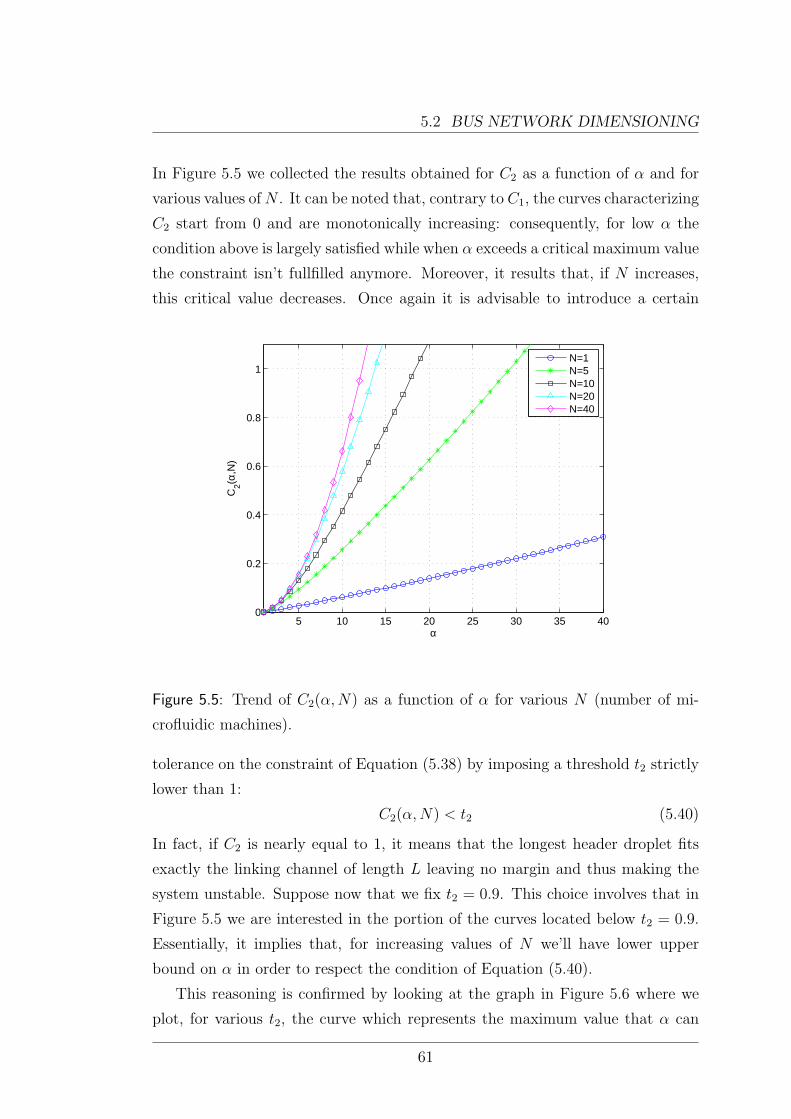
5.2 BUS NETWORK DIMENSIONING
In Figure 5.5 we collected the results obtained for C2 as a function of α and for
various values ofN . It can be noted that, contrary to C1, the curves characterizing
C2 start from 0 and are monotonically increasing: consequently, for low α the
condition above is largely satisfied while when α exceeds a critical maximum value
the constraint isn’t fullfilled anymore. Moreover, it results that, if N increases,
this critical value decreases. Once again it is advisable to introduce a certain
5 10 15 20 25 30 35 400
0.2
0.4
0.6
0.8
1
α
C2(α
,N)
N=1N=5N=10N=20N=40
Figure 5.5: Trend of C2(α,N) as a function of α for various N (number of mi-
crofluidic machines).
tolerance on the constraint of Equation (5.38) by imposing a threshold t2 strictly
lower than 1:
C2(α,N) < t2 (5.40)
In fact, if C2 is nearly equal to 1, it means that the longest header droplet fits
exactly the linking channel of length L leaving no margin and thus making the
system unstable. Suppose now that we fix t2 = 0.9. This choice involves that in
Figure 5.5 we are interested in the portion of the curves located below t2 = 0.9.
Essentially, it implies that, for increasing values of N we’ll have lower upper
bound on α in order to respect the condition of Equation (5.40).
This reasoning is confirmed by looking at the graph in Figure 5.6 where we
plot, for various t2, the curve which represents the maximum value that α can
61

5. DESIGN AND PERFORMANCE OF A MICROFLUIDIC BUSNETWORK
assume as a function of N .
0 5 10 15 20 25 300
10
20
30
40
50
60
70
80
90
100
N
α max
t2=0.5
t2=0.7
t2=0.9
Figure 5.6: Maximum value of α imposed by Equation (5.40) as a function of N
for various thresholds t2.
The two constraints analyzed so far are clearly in contraposition with each
other: the former (Equation (5.29)), in fact, imposes a minimum α while the latter
(Equation (5.40)) fixes a maximum value for the same prameter. In Figure 5.7 we
report the graph obtained combining and processing both the curves in Figure 5.4
and in Figure 5.6.
The conclusions that can be drawn are that, fixing the thresholds t1 and
t2,4 there exists a specific region where the problem has solution (i.e., the area
enclosed by the couples of curves with the same shape in Figure 5.7). Beyond
this range no solution can be found. Consequently, the point where the two
curves above intersect discriminates between the systems with solution and with
no solution: αmin, in fact, must always stay under αmax in order to respect both
constraints. Therefore, for N higher than the value of the abscissa where the two
4In our study we choose, for convenience, the same t1 and t2 though, obviously, they might
be selected independently.
62

5.2 BUS NETWORK DIMENSIONING
0 5 10 15 20 25 300
10
20
30
40
50
60
70
80
90
100
N
α
t1=t
2=0.5
t1=t
2=0.7
t1=t
2=0.9
Figure 5.7: Minimum and maximum values of α imposed respectively by Equation
(5.29) and (5.40) as a function of N for various thresholds t1 = t2.
curves cross each other, no solution can be found and, in such a situation, we
may only proceed in two ways:
we can choose a lower number of microfluidic machine N for our network,
losing, however, in system scalability;
we can loosen the bonds of Equations (5.29) and (5.40) selecting two new
thresholds t1 and t2 greater than the previous ones. Accordingly, however,
we’ll lose in system robustness.
The last condition we have to satisfy in our model derives from the droplet
generator we have chosen for our network. In fact, looking at the Equation (3.6),
which defines the droplets length achievable by means of a cross-flowing generator
in squeezing regime, it results that we cannot produce droplets shorter than w
(with w being the width of the channels). This means that all the header droplets
we consider need to be longer than w:
Ldn > w, ∀n = 1, ..., N (5.41)
63

5. DESIGN AND PERFORMANCE OF A MICROFLUIDIC BUSNETWORK
which corresponds to impose:
minLdn > w (5.42)
We have already seen that minLdn = Ld1 , so, it becomes:
Ld1 > w (5.43)
Now, substituting Equation (5.11), we get:
δr1wh3
(µd − µc)a> w ⇒ δr1 >
(µd − µc)a
h3(5.44)
Remembering Equation (5.6), it results that condition necessary but not sufficient
to satisfy this constraint is:
R1
(1− 1
α
)>
(µd − µc)a
h3(5.45)
Finally, exploiting Equation (5.5), we obtain
R >(µd − µc)a
(α− 1)h3(5.46)
So, once we select the suitable parameter α thanks to the graph of Figure 5.7,
we’ll consequently have a specific lower bound for the resistance of the linking
channels in our network. It can be noted that if α increases it is easier to fullfil
the previous condition. An increment in this parameter, in fact, corresponds to
having more unbalancing between Rn and Req,n (see Equation (5.5)), thus leading
to use longer header droplets in order to deviate the payload in the right branch.
In this way, it is more likely that we need header droplets longer than w.
5.3 Bus network performance
In the previous section we focused our attention on studying the concepts and
requirements useful to opportunely size a microfluidic bus network such as the
one in Figure 5.1. However, a key aspect is still missing before we can move to
illustrate of the system performance. The latters, in fact, are strongly affected
by a parameter that we haven’t considered yet: the input velocity u of the liquid
flows in the network. It is patent that, as u increases we will have a corresponding
higher “throughput” and vice versa.
64

5.3 BUS NETWORK PERFORMANCE
Accordingly, we need to find the physical constraints that rule the maximum
input velocity (u) sustainable by our network, or, equivalently, the maximum flow
rate (Q) since Q = u∗w∗h where w is the width of the channel and h is its height.
Of course, this quantity is influenced by both the necessity of having laminar flow
and, thus, low Reynolds number (see Section §2.3) in a microfluidic system and
preventing flow degeneration in droplet production (see Section §3.3.2). However,
for the typical flow velocities of microfluidic devices (up to tens of mm/s), these
requirements are largely satisfied.
Actually, there is another aspect which limits u the most, i.e. the requirement
of maintaining the integrity of the drops in correspondence of the bifurcations (see
Section §4.1).5 Let’s, in fact, consider Equation (4.1) which discriminates between
breakup and non-breakup regime in a T-junction. Specifically, in order to avoid
the split of the droplet, we need to satisfy the condition:
Ld
w< χCa−0.21 (5.47)
Now, it is appropriate to express Ca as µcuσ
(see Section §2.2). In this way, in
fact, it is evident its dependance on u. So, substituting it in Equation (5.47), we
get:Ld
w< χ
(µcu
σ
)−0.21
(5.48)
and, inverting the previous formula, we finally obtain:
u <σ
µc
(χw
Ld
) 10.21
(5.49)
This result tells us that, in general, the maximum input velocity u is limited
by both the physical properties of the dispersed and continuous phase (σ, µc,
χ which depends on the ratio µd
µcand Ld) and the geometry of the system (w).
However, realistically, the only parameters that may vary in the network are σ, χ
and Ld. The former two depends on the substance that constitutes the dispersed
phase but, so as not to weigh down the notation, hereafter we’ll consider them
constant and equal for both the header and the payload droplets.6 Conversely,
Ld (the length of the droplets) is intrinsically a highly changeable parameter.
5It is important to notice that, at the first bifurcation of Figure 5.1, uc = ud = u which is the
velocity setted by the droplet generator. Furthermore, uc ≤ u throughout the entire network,
as a consequence of Kirchhoff’s current law.6The generalization of this case is, anyway, elementary.
65

5. DESIGN AND PERFORMANCE OF A MICROFLUIDIC BUSNETWORK
Following this reasoning, in Figure 5.8 we reported the typical trend of the
maximum velocity (u) allowed by the system as a function of the droplets length
(Ld) in order to avoid their breakup at the bifurcations. The other reference
parameters considered here are: µc = 1.002mPa·s, µd = 145.5mPa·s, χ = 0.187,
w = 150 µm and σ = 46 mN/m.
3 4 5 6 7 8
x 10−4
0.5
1
1.5
2
2.5
3
3.5
4
4.5
5
5.5
x 10−4
Ld [m]
u [m
/s]
Figure 5.8: Maximum input velocity u allowed for the system as a function of the
droplet’s length Ld.
Analyzing the graph in Figure 5.8, we notice that u decreases drastically as
soon as Ld increases a bit. The latter parameter will, thus, impact strongly on
the throughput of the network.
On this purpose, we have seen in Section §5.2 that the header droplet’s length
varies depending on the number of microfluidic machines (N) in the network
and the destination of the payload drop in accordance with Equation (5.11).
Specifically, we have realized that we need longer header droplets as N increases.
Therefore, the system performance will expire quickly once we add microfluidic
machines to the network.
The payload droplet’s length, in turn, is defined by the volume of liquid that
we want to convey to the microfluidic machine. Now, referring to Equation (5.49),
it follows that the longest droplet injected in the system controls the maximum
66

5.3 BUS NETWORK PERFORMANCE
inlet velocity u allowed. So, as long as the payload droplet is shorter than the
header droplet (LH) the maximum u is fixed by the condition:
u <σ
µc
(χw
LH
) 10.21
(5.50)
while, if the length of the payload droplet LP exceeds LH , we get:7
u <σ
µc
(χw
LP
) 10.21
(5.51)
5.3.1 Numerical results
At the end of this dissertation, we are finally able to completely configure the
generical microfluidic bus network of Figure 5.1 by setting all its appropriate
geometrical and physical parameters. Consequently, we can extract the time re-
quired to forward any payload droplet to the target microfluidic machines and,
thus, evaluate the “throughput” of the network which is the main aim of the
present Section. However, we must first choose a sensible way to define the con-
cept of throughput in a microfluidic system. Reasoning by analogy with the
world of telecommunications, the “packets” we want to deliver in a microfluidic
network are represented by the droplets. Furthermore, remembering that packets
in telecommunication networks are usually weighed according to the amount of
information they transport (number of bits), we’ll reasonably have to weigh the
droplets in microfluidic networks by the amount of substance they carry (volume
of liquid). Hence, hereafter, we’ll express the throughput in the microfluidic con-
text as the volume of fluid delivered to the output nodes (microfluidic machines)
per unit time denoting it with the symbol R [m3/s].
Another dutiful premise, before illustrating the results, concerns the protocol
we used to commit resources in our system, i.e. the scheduling policy used to
inject droplets in the network. In this regard, we chose the crudest but, at the
same time, simplest possible solution which, in practice, consists in sending a
couple of header/payload droplets at a time and wait until they have completely
left the system before injecting the next one. This rule (a sort of “Stop & Wait”
protocol) ensures that the droplets will follow the theoretical dynamics previously
exposed. The presence of additional droplets in the systems may, in fact, affect
7This is true only if we use the same substances for header and payload droplets.
67

5. DESIGN AND PERFORMANCE OF A MICROFLUIDIC BUSNETWORK
negatively the behavior of the other bubbles, leading to unexpected results. In
this regard, we remember that a droplet arriving at a junction, if it does not
break, usually goes to the outlet characterized by the highest flow rate. Since
droplets can increase hydrodynamic resistance of a channel, the presence of addi-
tional droplets downstream in each outlet arm can affect the respective flow rates
and, therefore, the partitioning at the bifurcation. This collective hydrodynamic
feedback modulated by the increased flow resistance introduced by the droplets
can alter the probability of partitioning and, thus, governs the traffic in capillary
tubes.
Thus, implementing the “Stop & Wait” protocol, in order to calculate the
mean throughput of a generic network with N microfluidic machines we proceed
in the following way:
We fix a uniform length for the payload droplets and size the network basing
on the theoretical background seen in the previous sections.
We reckon the times required to reach each microfluidic machine of the
network applying the “Stop & Wait” protocol already described. This could
be done by simulating, one at a time, the flow of each pair header/payload.8
In particular, we obtain, with the aid of Matlab, the so called busy period
bi, ∀i = 1, ..., N which is the time during which at least one the two droplets
(header and payload) occupies the system. Clearly, it also coincides with
the time we have to wait before injective the successive bubbles due to the
“Stop & Wait” mechanism.
We average these results out of all the destinations, obtaining the mean
busy time to reach a microfluidic machines in the referring network: B =∑Ni=1 bipi, where pi is the probability of having a payload droplet destined
to the i-th microfluidic machine. Hereafter we’ll assume a discrete uniform
distribution whereby pi =1N, ∀i = 1, ..., N .
We make the ratio between the volume of the payload droplets and the
mean busy period obtaining the desired mean throughput of the network:
R = V olB.
8We remember that we need different header droplets in order to deviate the payload droplet
to different microfluidic machines.
68

5.3 BUS NETWORK PERFORMANCE
In Figure 5.9 we collect the results obtained for systems with 2, 3, 4 and
5 microfluidic machines considering, from time to time, payload droplets with
length equal to LdN , i.e. the length of the corresponding biggest header droplet
of the network. This entails that the maximum input velocity (u) associated to the
network is always limited by the payload length (in fact, LP ≥ Ldn ∀n = 1, ..., N)
in accordance with Equation (5.51).
The general performance ahieved are quite low. This is because we used wide
margins to comply the conditions expressed by Equations (5.29) and (5.40), at
the expense of throughput. Moreover, the dispersed phase chosen had a very
high dynamic viscosity compared to the continuous phase. This implies that we
inject in the network a fluid very reluctant to motion (see Section §2.1) which
increases considerably the resistance of the channel it occupies and thus decreases
the corresponding flow rate. Furthermore, as we already stated, since µd ≫ µc,
the parameter χ in Equation (5.49) is accordingly quite low. This acts, again, as
a detriment to performance by limiting significantly the input velocity u of the
system.
1.5 2 2.5 3 3.5 4 4.5 5 5.50
0.5
1
1.5
2
2.5x 10
−15
N
R [m
3 /s]
Figure 5.9: Mean throughput of the microfluidic bus network as a function of N
for a single payload droplet.
As we expected, the “capacity” of the network expires quickly as N increases.
69

5. DESIGN AND PERFORMANCE OF A MICROFLUIDIC BUSNETWORK
This is due to three main reasons:
If we augment N we’ll necessarily have greater networks and, thus, the
droplets will have to face longer paths before leaving the system.
In turn, the “Stop & Wait” model adopted to manage the entry of droplets
in the systems, strongly penalizes networks with many microfluidic ma-
chines. In fact, as we already discussed, it doesn’t provide for the simulta-
neous sending of multiple payload droplets. In this way, we’ll have to wait
longer before injecting the next payload droplet, as N increases.
Finally, we have already argued that, once we add microfluidic machines in
the system, we’ll need corresponding longer header droplets according to
Equation (5.11). This will limit the maximum input velocity of the system
(see Equation (5.49)) affecting, once again, negatively the throughput of
the network.
To conclude our analysis, in Figure 5.10 has been reported the graph, analo-
gous to that of Figure 5.9, obtained by splitting the payload droplet previously
considered in two sub-droplets with halved length. In practice, compared to the
former case, we have transmitted the same volume of fluid to the microfluidic ma-
chines by injecting two bubbles with halved length. The latters, of course, have
been sent in two separate sessions because of the “Stop & Wait” model adopted.
The results show a fairly good improvement in the throughput (see Fig-
ure 5.11). This could seem counterintuitive since, by halving the payload droplet,
we need to forward the resulting pair of sub-droplets in two separate tranche due
to the “Stop & Wait” protocol while, in the previous case, a single transmis-
sion was sufficient to convey the same volume of fluid to the desired microfluidic
machine. However, the reduced dimension of the payload droplets allows us to
increase the input velocity of the system in accordance with Equation (5.49).
Moreover, as we have already seen, by decreasing the length of the droplets we
will also introduce “less resistance” in the channels they occupy and, consequently,
the bubbles will move faster. In the case just described, the union of these two
factors prevails over the burden of sending droplets in two rounds and, thus, is
explained the throughput gain observed.
Therefore, if we have a very long payload droplet, this result tells us that it is
convenient to split it in numerous sub-droplets and send them one at a time along
70
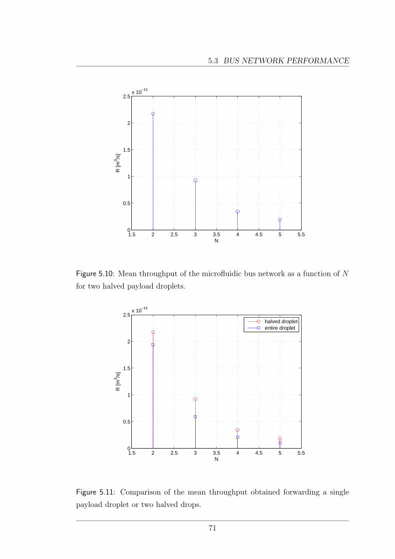
5.3 BUS NETWORK PERFORMANCE
1.5 2 2.5 3 3.5 4 4.5 5 5.50
0.5
1
1.5
2
2.5x 10
−15
N
R [m
3 /s]
Figure 5.10: Mean throughput of the microfluidic bus network as a function of N
for two halved payload droplets.
1.5 2 2.5 3 3.5 4 4.5 5 5.50
0.5
1
1.5
2
2.5x 10
−15
N
R [m
3 /s]
halved dropletentire droplet
Figure 5.11: Comparison of the mean throughput obtained forwarding a single
payload droplet or two halved drops.
71
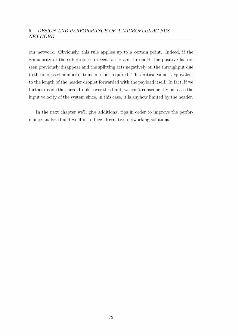
5. DESIGN AND PERFORMANCE OF A MICROFLUIDIC BUSNETWORK
our network. Obviously, this rule applies up to a certain point. Indeed, if the
granularity of the sub-droplets exceeds a certain threshold, the positive factors
seen previously disappear and the splitting acts negatively on the throughput due
to the increased number of transmissions required. This critical value is equivalent
to the length of the header droplet forwarded with the payload itself. In fact, if we
further divide the cargo droplet over this limit, we can’t consequently increase the
input velocity of the system since, in this case, it is anyhow limited by the header.
In the next chapter we’ll give additional tips in order to improve the perfor-
mance analyzed and we’ll introduce alternative networking solutions.
72

Chapter 6
Future developments
The topic covered in this thesis lends itself easily to improvements and future
developments. Among them, a couple of interesting proposals will be briefly
discussed in this conclusive chapter.
6.1 Scheduling
In order to enhance the performance of the bus network previously described, it
might be thought to a more sophisticated scheduling algorithm, compared to the
“Stop &Wait” one, able to manage opportunely the contemporaneous presence of
more than one payload droplet in the system. This scenario, unfortunately, entails
an exponential increment in the complexity of the system itself. In fact, we’ve
already seen that every drop raises the hydrodynamic resistance of the channel
that contains it. Therefore, whenever we inject additional droplets in the network,
we vary the volumetric flow rate of the corresponding channel and, cascading, the
distribution of the flow rates downstream in each parallel arm. This collective
hydrodynamic feedback modulated by the increased flow resistance introduced by
the droplets can alter the probability of partitioning and, thus, governs the traffic
in capillary tubes leading, in the worst case, to uncontrollable “fluctuations”.
However, if kept under control, we could exploit in our behalf such a presence
of numerous droplets in the network. Suppose, in fact, that we want to deliver a
single droplet to each microfluidic machine connected to the network of Figure 5.1.
With the “Stop & Wait” protocol introduced in the previous Chapter we would
have to inject a pair of droplets header/payload at a time, wait until they left the
73
6. FUTURE DEVELOPMENTS
system and then forward the next one.
Conversely, with a more sophisticated scheduler, we could achieve the same
goal by injecting toghether all of the payload droplets in the network. This,
in fact, would lead to the formation of a train of droplets where the first ones
can act as header droplets for the following ones redirecting them to the target
microfluidic machines as we saw in Section §4.2. Obviously, this brainwave re-
quires a more thorough analysis of the network and works only if we synchronize
opportunely the forwarding of the droplets.
On the other hand, the benefits compared to the “Stop & Wait” algorithm
are numerous:
we can save in terms of physical resources because we don’t need anymore
to employ a dedicated header droplet for each payload droplet but rather
use the payload itself to deviate the following drops;
we can gain in terms of throughput because we are not forced anymore to
wait for the payload droplet to reach its destination before forwarding a
new one;
we are able to commit more effectively the network resources. In this new
scenario, in fact, we can convey simultaneously the droplets to the microflu-
idic machines which can, thus, work in parallel.
6.2 Network topology
Lastly, another interesting flexibility aspect which characterizes a microfluidic
network concerns its topology. The bus geometry introduced in this work, in
fact, is only one of the configuration that the system may assume. Indeed, at
such scale, it is possible to reassemble the network in many different ways de-
pending on our purpose. For instance, a tree-shaped geometry (see Figure 6.1)
could be suitably implemented in order to arrange hierarchically the microfluidic
machines in the system.
At the end of this thesis it is evident how microfluidics offers great - perhaps
even revolutionary - new capabilities for the future. However, a great deal of
work remains to be done before it can be claimed to be more than an active
74

6.2 NETWORK TOPOLOGY
Q
MM # 1
MM # 2
MM # 3
MM # 4
MM # 5
MM # 6
MM # 7
MM # 8
Figure 6.1: Design of a microfluidic tree network.
field of academic research. Nonethless, the fundamentals of the field are very
strong: much of the world’s technology requires the manipulation of fluids, and
extending those manipulations to small volumes, with precise dynamic control
over concentrations, while discovering and expoliting new phenomena occurring
in fluids at the microscale level must, ultimately, be very important.
75

Appendix A
OpenFOAM
OpenFOAM (Open Source Field Operation and Manipulation) is a free, open
source software package developed by OpenCFD Ltd at ESI Group and dis-
tributed by the OpenFOAM Foundation. Basically it works as a C++ toolbox for
the creation of customized numerical solvers, and pre-/post-processing utilities
for the solution of continuum mechanics problems, including computational fluid
dynamics (CFD).
In the present thesis, we presented a microfluidic study using OpenFOAM to
simulate many of the processes described. In particular, the solver to which we
have referred is called interFoam.
We have used the Volume of Fluid (VoF) method to model the flow of two
immiscible fluid (dispersed and continuous phase). In VoF a single set of Navier-
Stokes equations for both phases is combined with an advection equation for
the fluid fraction α of one of the fluids. In the present work, it is important to
underline that both phases are assumed incompressible and Newtonian and the
flow is assumed laminar. Hence the general governing equations can be written
as: ∇U = 0∂ρU∂t
+∇ · (ρUU) = −∇p+∇ · µ(∇U +∇UT ) + ρF + FS
∂α∂t
+∇ · (αU)−∇ · (α(1− α)Ur) = 0
(A.1)
where U is the fluid velocity, p is the pressure, ρ the density, µ the viscosity, F
a body force and α the volume fraction, which is one in the the bulk of fluid
1 (dispersed phase), zero in the bulk of fluid 2 (continuous phase), and has an
77

APP. A OPENFOAM
intermediate value in near the interface between the two fluids. FS, instead, is
the surface tension force, modeled as a volumetric force active in the vicinity of
the interface only, as described below. The bulk density ρ and viscosity µ in the
above Equation (A.1) are computed as weighted averages of two phase properties,
based on the fluid fraction α.
The fluid interface is sharpened by introducing the artificial compression term
∇ · (α(1−α)Ur) in the last formula of Equation (A.1), in which Ur describes the
artificial compression velocity. This term acts to counteract interface diffusion
and is active only on the fluid interface.
The interfacial tension force is approximated as a body force active in inter-
facial grid cells only, and is formulated as FS = σκ(∇α) where σ is the interfacial
tension coefficient and κ = ∇ · (∇α/|∇α|) is the curvature of the interface.
The PIMPLE scheme is applied for pressure-velocity coupling. We used a first
order Euler scheme for the transient terms, controlling the time step by setting
the Courant maximum number to 0.9. Courant number reflects the portion of a
cell that a solute will traverse by advection in one time step and is defined as:
Co =u∆t
∆l(A.2)
where ∆l is the dimension of the grid cell at each location, u is the average
linear velocity at that location and ∆t is the maximum time step size. When
advection dominates dispersion, designing a model with Co < 1 will decrease
oscillations, improve accuracy and decrease numerical dispersion. Therefore, we
are interested in satisfying this condition. A first Gauss linear scheme was used
for the discretization of the gradient terms.
The geometry of the three-dimensional channel used has fixed common param-
eters. In particular, we imposed an uniform width and height for every channel
equal to w = 150µm and h = 50µm respectively. The computational domains
and meshes were generated with blockMesh, an internal mesh generator of Open-
FOAM while the graphical results were viewed using ParaView (an open source
mutiple-platform application for interactive, scientific visualization).
78

Bibliography
[1] W. O. Kwang, L. Kangsun, A. Byungwook and E. P. Furlani, “Design of
pressure-driven microfluidic networks using electric circuit analogy”, Lab
Chip, 12, 515-545, 2012.
[2] C. N. Baroud, F. Gallaire and R. Dangla, “Dynamics of microfluidic
droplets”, Lab Chip, 10, 2032-2045, 2010.
[3] C. Cramer, P. Fischer and E. J. Windhab, “Drop formation in a co-flowing
ambient fluid”, Chem. Eng. Sci., 59, 3045-3058, 2004.
[4] D. Funfschilling, H. Debas, H. Z. Li and T. G. Mason, “Flow-field dynamics
during droplet formation by dripping in hydrodynamic-focusing microflu-
idics”, Phys. Rev. E., 80, 15301, 2009.
[5] W. Lee, L. M. Walker and S. L. Anna, “Role of geometry and fluid properties
in droplet and thread formation processes in planar flow focusing”, Phys.
Fluids, 21, 032103, 2009.
[6] H. A. Stone, “On lubrication flows in geometries with zero local curvature”,
Chem. Eng. Sci., 60, 4838-4845, 2005.
[7] T. Thorsen, R.W. Roberts, F. H. Arnold and S. R. Quake, “Dynamic pattern
formation in a vesicle-generating microfluidic device”, Phys. Rev. Lett., 86,
4163-4166, 2001.
[8] P. Garstecki, M. J. Fuerstman, H. A. Stone and G. M. Whitesides, “For-
mation of droplets and bubbles in a microfluidic T-junction - scaling and
mechanism of break-up”, Lab Chip, 6, 437-446, 2006.
79

BIBLIOGRAPHY
[9] M. de Menech, P. Garstecki, F. Jousse and H. A. Stone, “Transition from
squeezing to dripping in a microfluidic T-shaped junction”, J. Fluid Mech.,
595, 141-161, 2008.
[10] M. J. Fuerstman, A. Lai, M. E. Thurlow, S. S. Shevkoplyas, H. A. Stone
and G. M. Whitesides, “The pressure drop along rectangular microchannels
containing bubbles”, Lab Chip, 7, 1479-1489, 2007.
[11] M.C. Jullien, M. J. Tsang Mui Ching, C. Cohen, L. Menetrier and P. Tabel-
ing, “Droplet breakup in microfluidic T-junctions at small capillary num-
bers”, Phys. Fluids, 21, 072001, 2009.
[12] A. Carlson, M. Do-Quang and G. Amberg, “Droplet dynamics in a bifurcat-
ing channel”, Int. J. Multiphase Flow, 36, 397-405, 2010.
[13] D. R. Link, S. L. Anna, D. A. Weitz and H. A. Stone, “Geometrically medi-
ated breakup of drops in microfluidic devices”, Phys. Rev. Lett., 92, 054503,
2004.
[14] A. M. Leshansky and L. M. Pismen, “Breakup of drops in a microfluidic T
junction”, Phys. Fluids, 21, 023303, 2009.
[15] S. Afkhami, A. M. Leshansky and Y. Renardy, “Numerical investigation
of elongated drops in a microfluidic T-junction”, Phys. Fluids, 23, 022002,
2011.
[16] E. De Leo, L. Galluccio, A. Lombardo and G. Morabito, “On the feasibility
of using microfluidic technologies for communications in Labs-on-a-Chip”.
To appear in Proc. of IEEE ICC 2012.
[17] D. A. Sessoms, M. Belloul, W. Engl, M. Roche, L. Courbin and P. Panizza,
“Droplet motion in microfluidic networks: Hydrodynamic interactions and
pressure-drop measurements”, Phys. Rev. E., 80, 016317, 2009.
80

Ringraziamenti
Ci tengo innanzitutto a ringraziare i miei genitori, a cui dedico questa tesi,
visto che senza il loro costante supporto e appoggio non sarei mai riuscito a rag-
giungere questo importante traguardo. Grazie, in particolare, per avermi sempre
sostenuto nelle mie scelte di vita, facili e difficili, senza mai farmele pesare e per
i saggi consigli e l’enorme affetto che non mi avete mai fatto mancare. Ringrazio
inoltre mia sorella, a cui tengo molto anche se non sempre lo dimostro a dovere,
per essere sempre presente quando ho bisogno di lei e per le parole di conforto
che sa dispensare nei momenti bui. Grazie anche a mio cugino Giovanni, con cui
sono cresciuto assieme, per il suo carattere che lo rende unico ed insostituibile e a
mia cugina Marina per le fenomenali ospitate a Bologna (ovviamente, per questo,
ringrazio anche a Massimo).
Un doveroso ringraziamento va poi al prof. Andrea Zanella, che reputo una
delle persone piu competenti ed appassionate nello svolgimento del proprio la-
voro. Lo ringrazio per gli utili suggerimenti e per le “lavagnate” di conti riempite
assieme senza i quali non sarei certo riuscito a portare a termine questa tesi.
Ringrazio Maria che, da quando ho ricordi, ha contribuito con grande affetto
a crescermi e a farmi diventare la persona che sono ora.
Ringrazio Francesco P. (Spazzola), Francesco L. (Sonda) e Chethan per la
forte e sincera amicizia che ci lega, per i pomeriggi di svago trascorsi assieme
e per le lunghe chiacchierate che hanno il notevole pregio di farmi dimenticare
i miei problemi. Grazie anche all’ inseparabile ed insostituibile compagnia del
mare che, anche se la vedo solo per un mese all’anno, riesce sempre a rendere
indimenticabili le mie estati.
Ringrazio inoltre i miei compagni di Universita, sia della triennale (soprat-
tutto Calle, Michi, Pelle, Davide e Valentina) che della magistrale (in particolare
Claudio, Silvia, Leo e Alex), per essere riusciti a rendere molto meno pesanti i
faticosi anni di studio di Ingegneria, e tutti gli “apprendisti Telecom” per rendere
il lavoro un’esperienza piacevole.
Infine, rivolgo un sincero ringraziamento alla persona con cui ho trascorso
tutta la vita e che piu di tutte mi capisce (d’altronde c’e “telepatia”), ovvero...a
mio gemello Alessandro.
Insomma, se ancora non si era capito, a tutti voi e a tutte le altre persone che
mi hanno sopportato e supportato volevo semplicemente dire: “grazie di esistere”.
81