milton armando sobre a aplica˘c~ao de t ecnicas de...

Universidade de AveiroDepartamento deElectronica, Telecomunicacoes e Informatica,

2014

Milton ArmandoCunguara

Sobre a aplicacao de Tecnicas de Controlo emRedes Industriais com Falhas

On the Application of Optimal Control Techniquesin Lossy Fieldbuses

“New problems cannot besolved using the old thinkingthat created them”

— Albert Einstein


2014


Sobre a aplicacao de Tecnicas de Controlo emRedes Industriais com Falhas

On the Application of Optimal Control Techniquesin Lossy Fieldbuses


2014


Sobre a aplicacao de Tecnicas de Controlo Optimoem Redes Industriais

Dissertacao apresentada a Universidade de Aveiro para cumprimento dosrequisitos necessarios a obtencao do grau de Doutor em Engenharia Elec-trotecnica, realizada sob orientacao cientıfica dos Professores Doutor TomasAntonio Mendes Oliveira e Silva, Professor associado do DepartamentoElectronica, Telecomunicacoes e Informatica da Universidade de Aveiro, ePaulo Bacelar Reis Pedreiras, Professor Auxilar do mesmo Departamento.

o juri / the jury

presidente / president Antonio Manuel Rosa Pereira CaetanoProfessor Catedratico da Universidade de Aveiro (por delegacao do Reitor da Uni-

versidade de Aveiro)

vogais / examiners committee Ana Lusa Lopes AntunesProfessora Adjunta do Instituto Superior Tecnico de Setubal

Luıs Miguel Pinho de AlmeidaProfessor associado da Universidade do Porto

Alexandre Manuel Moutela Nunes da MotaProfessor Associado da Universidade de Aveiro

Tomas Antonio Mendes Oliveira e Silva (orientador)Professor Associado da Universidade de Aveiro

agradecimentos /acknowledgements

. . . a todos os que me apoiaram durante este percurso, em especial, aosmeus familiares.

Aos meus orientadores. . .

Aos membros do juri por terem encontrado tempo para rever e comentaresta humilde tese.

Ao governo da republica portuguesa, que atraves da Fundacao para aCiencia e a Tecnologia, por meio da Bolsa de Doutoramento de contractonumero SFRH/BD/62178/2009/J53651387T4E, ajudou financeiramente arealizacao desta tese. Igualmente, agradeco ao governo da republica por-tuguesa, que atraves do Projecto Serv-CPS, prestou ajuda financeira queconduziu a aquisao de bens materiais que foram de vital importancia paraa execucao desta tese.

A todos os que nao tendo sido acima mencionados, tenham contribuıdopositivamente para a realizaccao desta tese.

Palavras-chave controlo, controlo optimo, controlo em rede, redes industriais, redes comfalhas

Resumo Em resultado de varias tendencias que tem afetado o mundo digital, o de-sempenho das redes de comunicacao em tempo-real esta continuamente aser melhorado. No entanto, tais tendendencias nao so introduzem melho-rias, como tambem introduzem uma serie de nao idealidades, tais como alatencia, o jitter da latencia de comunicacao e uma maior probabilidade deperda de pacotes.

Esta tese tem o seu cerne em falhas de comunicacao que surgem em taisredes, sob o ponto de vista do controlo automatico. Concretamente, saoestudados os efeitos das perdas de pacotes em redes de controlo, bem comoarquitecturas e tecnicas optimas de compensacao das mesmas.

Primeiramente, e proposta uma nova abordagem para colmatar os proble-mas que surgem em virtude de tais perdas. Essa nova abordagem e baseadano envio simultaneo de varios valores numa unica mensagem. Tais men-sagens podem ser de sensor para controlador, caso em que as mesmas saoconstituıdas por um conjunto de valores passados, ou de controlador paraactuador, caso em que tais mensagens contem estimativas de futuros valoresde controlo. Uma serie de testes revela as vantagens de tal abordagem.

A abordagem acima explanada e seguidamente expandida de modo a aco-modar o controlo optimo. Contudo, ao contrario da abordagem acimaapresentada, que passa pelo nao envio deliberado de certas mensagens comvista a alcancar um uso mais eficiente dos recursos de rede; no presentecaso, as tecnicas sao usadas para reduzir os efeitos da perda de pacotes.

Em seguida sao estudadas abordagens de controlo optimo que em situacoesde perda de pacotes empregam formas generalizadas da aplicacao de val-ores de saıda. Este estudo culmina com o desenvolvimento de um novocontrolador optimo, bem como a funcao, entre as funcoes generalizadasdo funcionamento do actuador, que conduz o sistema a um desempenhooptimo.

E tambem apresentada uma linha de investigacao diferente, relacionada coma oscilacao da saıda que ocorre em consequencia da utilizacao de tecnicas ealgoritmos classicos de co-desenho de controlo e redes industriais. O algo-ritmo proposto tem como finalidade permitir que tais algoritmos classicospossam ser executados sem causar oscilacoes de saıda, oscilacoes que porsua vez aumentam o valor da funcao de custo. Tais aumentos da funcaodo custo, podem, em certas circunstancias, por em causa os benefıcios daaplicacao das tecnicas de co-desenho classico.

Resumo (Continuacao) Numa outra linha de investigacao, foram estudadas formas, mais eficientesque as contemporaneas, de geracao de sequencias de execucoes de tare-fas que garantam que pelo menos um dado numero de tarefas activadasserao executadas por cada conjunto contıguo composto por um numeropredefinido de activacoes. Esta tecnica podera, no futuro, ser aplicada nageracao dos padroes de envio de mensagens que e empregue na abordagemde utilizacao eficiente dos recursos de rede acima referida. A tecnica pro-posta de geracao de tarefas e melhor que as anteriores no sentido em quea mesma e capaz de escalonar sistemas que nao sao escalonaveis pelastecnicas classicas.

A tese tambm apresenta um mecanismo que permite fazer o encamin-hamento multi-caminho em redes de sensores sem fios com falhas semcausar a contagm em duplicado. Assim sendo a mesma tecnica melhorao desempenho das redes de sensores sem fios, tornando as mesmas maismaleavel as necessidades do controlo aumatico em redes sem fios.

Como foi referido acima, a tese foca-se em tecnicas de melhoria de de-sempenho de sistemas de controlo distribuıdo em que os varios elementosde controlo encontram-se interligados por meio de uma rede industrial quepode estar sujeita a perda de pacotes. As primeiras tres abordagens cingem-se a este tema, sendo que primeiras duas olham para o problema sob umponto de vista arquitetural, enquanto que a terceira olha sob um ponto devista mais teorico. A quarta abordagem garante que outras propostas quepodem ser encontradas na literatura e que visam atingir resultados semel-hantes aos que se pretendem atingir nesta tese, possam faze-lo sem causaroutros problemas que invalidem as solucoes em questao. Seguidamente, eapresenta-se uma abordagem ao problema proposto nesta tese que foca-sena geracao eficiente de padroes para subsequente utilizacao nas abordagensacima referidas. E por fim, apresentar-se-a uma tecnica de optimizacao dofuncionamento de redes sem fios que promete melhorar o controlo em taisredes.

Palavras-chave Control, Optimal control, Networked control, Real-time networks, Field-buses, Lossy Networks

Abstract The performance of real-time networks is under continuous improvement asa result of several trends in the digital world. However, these tendencies notonly cause improvements, but also exacerbates a series of unideal aspectsof real-time networks such as communication latency, jitter of the latencyand packet drop rate.

This Thesis focuses on the communication errors that appear on such real-time networks, from the point-of-view of automatic control. Specifically, itinvestigates the effects of packet drops in automatic control over fieldbuses,as well as the architectures and optimal techniques for their compensation.

Firstly, a new approach to address the problems that rise in virtue of suchpacket drops, is proposed. This novel approach is based on the simultaneoustransmission of several values in a single message. Such messages canbe from sensor to controller, in which case they are comprised of severalpast sensor readings, or from controller to actuator in which case they arecomprised of estimates of several future control values. A series of testsreveal the advantages of this approach.

The above-explained approach is then expanded as to accommodate thetechniques of contemporary optimal control. However, unlike the afore-mentioned approach, that deliberately does not send certain messages inorder to make a more efficient use of network resources; in the second case,the techniques are used to reduce the effects of packet losses.

After these two approaches that are based on data aggregation, it is alsostudied the optimal control in packet dropping fieldbuses, using generalizedactuator output functions. This study ends with the development of a newoptimal controller, as well as the function, among the generalized func-tions that dictate the actuator’s behaviour in the absence of a new controlmessage, that leads to the optimal performance.

The Thesis also presents a different line of research, related with the outputoscillations that take place as a consequence of the use of classic co-designtechniques of networked control. The proposed algorithm has the goal ofallowing the execution of such classical co-design algorithms without causingan output oscillation that increases the value of the cost function. Suchincreases may, under certain circumstances, negate the advantages of theapplication of the classical co-design techniques.

Abstract (Continuation) A yet another line of research, investigated algorithms, more efficient thancontemporary ones, to generate task execution sequences that guaranteethat at least a given number of activated jobs will be executed out ofevery set composed by a predetermined number of contiguous activations.This algorithm may, in the future, be applied to the generation of messagetransmission patterns in the above-mentioned techniques for the efficientuse of network resources. The proposed task generation algorithm is betterthan its predecessors in the sense that it is capable of scheduling systemsthat cannot be scheduled by its predecessor algorithms.

The Thesis also presents a mechanism that allows to perform multi-pathrouting in wireless sensor networks, while ensuring that no value will becounted in duplicate. Thereby, this technique improves the performance ofwireless sensor networks, rendering them more suitable for control applica-tions.

As mentioned before, this Thesis is centered around techniques for theimprovement of performance of distributed control systems in which severalelements are connected through a fieldbus that may be subject to packetdrops. The first three approaches are directly related to this topic, with thefirst two approaching the problem from an architectural standpoint, whereasthe third one does so from more theoretical grounds. The fourth approachensures that the approaches to this and similar problems that can be foundin the literature that try to achieve goals similar to objectives of this Thesis,can do so without causing other problems that may invalidate the solutionsin question. Then, the thesis presents an approach to the problem dealtwith in it, which is centered in the efficient generation of the transmissionpatterns that are used in the aforementioned approaches.

Contents

Contents i

List of Figures vii

List of Tables ix

1 Introduction 11.1 Motivation . . . . . . . . . . . . . . . . . . . . . . . . . . . . . . . . . . . . . 11.2 Assumptions . . . . . . . . . . . . . . . . . . . . . . . . . . . . . . . . . . . . 21.3 The Thesis . . . . . . . . . . . . . . . . . . . . . . . . . . . . . . . . . . . . . 31.4 Structure of the Dissertation . . . . . . . . . . . . . . . . . . . . . . . . . . . 51.5 Contributions of this Thesis . . . . . . . . . . . . . . . . . . . . . . . . . . . . 5

1.5.1 List of Publications . . . . . . . . . . . . . . . . . . . . . . . . . . . . 6

2 Background 92.1 Principles of System Representation . . . . . . . . . . . . . . . . . . . . . . . 9

2.1.1 Linearity . . . . . . . . . . . . . . . . . . . . . . . . . . . . . . . . . . 10Continuous-Time Representations . . . . . . . . . . . . . . . . . . . . 11Discrete-Time Representations . . . . . . . . . . . . . . . . . . . . . . 12Test Signals . . . . . . . . . . . . . . . . . . . . . . . . . . . . . . . . . 13

2.1.2 Discretization . . . . . . . . . . . . . . . . . . . . . . . . . . . . . . . . 15Output Signal “Analogization” . . . . . . . . . . . . . . . . . . . . . . 15Derivative Approximations . . . . . . . . . . . . . . . . . . . . . . . . 16

2.1.3 Stability . . . . . . . . . . . . . . . . . . . . . . . . . . . . . . . . . . . 192.2 State Space Representations . . . . . . . . . . . . . . . . . . . . . . . . . . . . 20

2.2.1 Static Non-Linearity . . . . . . . . . . . . . . . . . . . . . . . . . . . . 222.2.2 Linear Systems with Noise . . . . . . . . . . . . . . . . . . . . . . . . . 23

System Noise Discretization . . . . . . . . . . . . . . . . . . . . . . . . 242.2.3 Continuous-time Kalman Filter . . . . . . . . . . . . . . . . . . . . . . 262.2.4 Discrete-time Kalman Filters . . . . . . . . . . . . . . . . . . . . . . . 28

2.3 Control . . . . . . . . . . . . . . . . . . . . . . . . . . . . . . . . . . . . . . . 302.3.1 Modern Control . . . . . . . . . . . . . . . . . . . . . . . . . . . . . . 32

Lyapunov Stability and Equilibrium . . . . . . . . . . . . . . . . . . . 32Controllability and Observability . . . . . . . . . . . . . . . . . . . . . 32Pole placement . . . . . . . . . . . . . . . . . . . . . . . . . . . . . . . 33Linear Quadratic Regulators/Gaussian . . . . . . . . . . . . . . . . . . 34Pontryagin Minimum Principle and Bellman-Jacobi-Hamilton Theorem 37

i

Discrete-Time Linear Quadratic Regulators . . . . . . . . . . . . . . . 38

2.3.2 Receding Horizon Control . . . . . . . . . . . . . . . . . . . . . . . . . 40

Generalized Predictive Control . . . . . . . . . . . . . . . . . . . . . . 40

Model Predictive Control . . . . . . . . . . . . . . . . . . . . . . . . . 42

2.3.3 Send-on-Delta, Adaptive Sampling and Event-triggered Control . . . . 43

2.3.4 Co-design . . . . . . . . . . . . . . . . . . . . . . . . . . . . . . . . . . 50

3 Real-Time Systems 53

3.1 Real-time Systems . . . . . . . . . . . . . . . . . . . . . . . . . . . . . . . . . 53

3.1.1 Task Models . . . . . . . . . . . . . . . . . . . . . . . . . . . . . . . . 54

3.1.2 Classification of Real-Time Systems . . . . . . . . . . . . . . . . . . . 54

Static Vs Dynamic Priority Assignment . . . . . . . . . . . . . . . . . 54

Static Vs Dynamic Systems . . . . . . . . . . . . . . . . . . . . . . . . 55

Resource Schedulability . . . . . . . . . . . . . . . . . . . . . . . . . . 55

Online Vs Offline Scheduling . . . . . . . . . . . . . . . . . . . . . . . 56

Resource Sharing Control . . . . . . . . . . . . . . . . . . . . . . . . . 56

3.1.3 Scheduling Algorithms . . . . . . . . . . . . . . . . . . . . . . . . . . . 56

Rate Monotonic Scheduling . . . . . . . . . . . . . . . . . . . . . . . . 56

Deadline Monotonic Scheduling . . . . . . . . . . . . . . . . . . . . . . 58

Scheduling Tasks With Arbitrary Deadlines . . . . . . . . . . . . . . . 59

First Come First Served . . . . . . . . . . . . . . . . . . . . . . . . . . 59

Earliest Deadline First . . . . . . . . . . . . . . . . . . . . . . . . . . . 60

Least Slack First . . . . . . . . . . . . . . . . . . . . . . . . . . . . . . 61

Servers . . . . . . . . . . . . . . . . . . . . . . . . . . . . . . . . . . . 62

3.2 Real-Time Communication Networks . . . . . . . . . . . . . . . . . . . . . . . 63

3.2.1 Real-Time Communication Architecture . . . . . . . . . . . . . . . . . 63

3.2.2 Real-Time Communication Cooperation Models . . . . . . . . . . . . . 64

Traffic Model . . . . . . . . . . . . . . . . . . . . . . . . . . . . . . . . 65

3.2.3 Real-time Communication Medium Access Control . . . . . . . . . . . 66

3.2.4 Effects of Available Real-Time Communication Networks on Networked Control 67

3.2.5 Available Real-Time Communication Networks . . . . . . . . . . . . . 68

3.3 (m,k)-firm Systems . . . . . . . . . . . . . . . . . . . . . . . . . . . . . . . . . 68

3.3.1 Related Work . . . . . . . . . . . . . . . . . . . . . . . . . . . . . . . . 69

3.4 Feedback Scheduling . . . . . . . . . . . . . . . . . . . . . . . . . . . . . . . . 72

4 Network Decoupled Control Architecture 77

4.1 Introduction . . . . . . . . . . . . . . . . . . . . . . . . . . . . . . . . . . . . . 77

4.2 Architecture Rationale . . . . . . . . . . . . . . . . . . . . . . . . . . . . . . . 78

4.3 Description of the Architecture . . . . . . . . . . . . . . . . . . . . . . . . . . 79

4.3.1 Sampler . . . . . . . . . . . . . . . . . . . . . . . . . . . . . . . . . . . 79

4.3.2 Controller . . . . . . . . . . . . . . . . . . . . . . . . . . . . . . . . . . 80

4.3.3 Actuator . . . . . . . . . . . . . . . . . . . . . . . . . . . . . . . . . . 81

4.4 Related Work . . . . . . . . . . . . . . . . . . . . . . . . . . . . . . . . . . . . 81

4.5 Performance Assessment . . . . . . . . . . . . . . . . . . . . . . . . . . . . . . 83

4.6 Summary and Conclusion . . . . . . . . . . . . . . . . . . . . . . . . . . . . . 85

ii

5 Control over Lossy Networks 87

5.1 Introduction . . . . . . . . . . . . . . . . . . . . . . . . . . . . . . . . . . . . . 87

5.2 Related Work . . . . . . . . . . . . . . . . . . . . . . . . . . . . . . . . . . . . 89

5.3 Controller Design Rationale . . . . . . . . . . . . . . . . . . . . . . . . . . . . 91

5.4 Problem Statement and Solution . . . . . . . . . . . . . . . . . . . . . . . . . 93

5.4.1 Noise Filtering . . . . . . . . . . . . . . . . . . . . . . . . . . . . . . . 94

Innovation . . . . . . . . . . . . . . . . . . . . . . . . . . . . . . . . . . 94

Correction . . . . . . . . . . . . . . . . . . . . . . . . . . . . . . . . . . 96

5.4.2 Optimal Control over Lossy Networks — TCP-Like Protocols . . . . . 97

5.4.3 Optimal Control Over Lossy Networks — UDP-Like Protocols . . . . 98

5.5 Simulations and Results . . . . . . . . . . . . . . . . . . . . . . . . . . . . . . 98

5.5.1 Comparison with other solutions . . . . . . . . . . . . . . . . . . . . . 100

5.6 Summary and Conclusions . . . . . . . . . . . . . . . . . . . . . . . . . . . . . 101

6 Control over Lossy Networks with Generalized Linear Output 103

6.1 Introduction . . . . . . . . . . . . . . . . . . . . . . . . . . . . . . . . . . . . . 103

6.2 Related Work . . . . . . . . . . . . . . . . . . . . . . . . . . . . . . . . . . . . 104

6.3 Problem Definition and Notation . . . . . . . . . . . . . . . . . . . . . . . . . 106

6.4 Optimal Control over Output Zero Lossy Networks . . . . . . . . . . . . . . . 108

6.5 Optimal Control over Generalized Hold Lossy Networks . . . . . . . . . . . . 108

6.5.1 Recursive Matrix Derivation . . . . . . . . . . . . . . . . . . . . . . . . 109

6.5.2 Differential Matrix Derivation . . . . . . . . . . . . . . . . . . . . . . . 111

6.6 Discussion . . . . . . . . . . . . . . . . . . . . . . . . . . . . . . . . . . . . . . 113

6.6.1 Domain of Application . . . . . . . . . . . . . . . . . . . . . . . . . . . 114

6.7 Optimal Actuator State Transition Matrix . . . . . . . . . . . . . . . . . . . . 114

6.7.1 Computation of M∗kzk−1 . . . . . . . . . . . . . . . . . . . . . . . . . . 116

6.8 Comparison with the Block Transmission Architecture . . . . . . . . . . . . . 118

6.9 Evaluation . . . . . . . . . . . . . . . . . . . . . . . . . . . . . . . . . . . . . . 119

6.9.1 A First Order System . . . . . . . . . . . . . . . . . . . . . . . . . . . 119

6.10 Conclusion and Future Work . . . . . . . . . . . . . . . . . . . . . . . . . . . 120

7 Oscillation Free Controller Change 123

7.1 Introduction and Motivation . . . . . . . . . . . . . . . . . . . . . . . . . . . . 123

7.2 Related Work . . . . . . . . . . . . . . . . . . . . . . . . . . . . . . . . . . . . 124

7.3 Controller Adaptation through Period Switch . . . . . . . . . . . . . . . . . . 125

7.3.1 Types of Controller Change . . . . . . . . . . . . . . . . . . . . . . . . 125

7.3.2 Period Switch . . . . . . . . . . . . . . . . . . . . . . . . . . . . . . . . 126

7.3.3 Problem Formulation . . . . . . . . . . . . . . . . . . . . . . . . . . . 128

7.3.4 Proposed Solution . . . . . . . . . . . . . . . . . . . . . . . . . . . . . 129

7.3.5 Complexity of the methodology . . . . . . . . . . . . . . . . . . . . . . 132

7.3.6 Orthogonality with respect to control and scheduling . . . . . . . . . . 132

7.4 Evaluation of Proposed Solution . . . . . . . . . . . . . . . . . . . . . . . . . 133

7.5 Conclusion . . . . . . . . . . . . . . . . . . . . . . . . . . . . . . . . . . . . . 136

iii

8 Toward Deterministic Implementations of (m,k)–firm Schedulers 137

8.1 Introduction . . . . . . . . . . . . . . . . . . . . . . . . . . . . . . . . . . . . . 137

8.1.1 On the Use of (m,k)-firm Schedulers for Control Purposes . . . . . . . 138

8.2 Static (Circular) (m,k)-firm Schedulers . . . . . . . . . . . . . . . . . . . . . . 138

8.3 Dynamic (m,k)-firm Schedules . . . . . . . . . . . . . . . . . . . . . . . . . . . 140

8.3.1 Dynamic Scheduling of Optional Executions . . . . . . . . . . . . . . . 142

8.3.2 Precedence Rules . . . . . . . . . . . . . . . . . . . . . . . . . . . . . . 143

8.3.3 Shifting Mandatory Jobs . . . . . . . . . . . . . . . . . . . . . . . . . . 145

8.3.4 hiperframe Initialization . . . . . . . . . . . . . . . . . . . . . . . . . . 147

8.4 Examples of Dynamic Scheduling . . . . . . . . . . . . . . . . . . . . . . . . . 148

8.5 Comparison with Previous Solutions . . . . . . . . . . . . . . . . . . . . . . . 152

8.6 Static (m,k)-firm frames (Revisited) . . . . . . . . . . . . . . . . . . . . . . . 154

8.6.1 Optimal Statical (m,k)-firm Scheduling . . . . . . . . . . . . . . . . . 158

8.7 Conclusion . . . . . . . . . . . . . . . . . . . . . . . . . . . . . . . . . . . . . 158

9 Aggregation of Duplicate Sensitive Summaries 161

9.1 Introduction . . . . . . . . . . . . . . . . . . . . . . . . . . . . . . . . . . . . . 161

9.1.1 On the Use of In-Network Aggregation of Duplicate Sensitive Summaries for WSN Control Applications162

9.2 Related Work . . . . . . . . . . . . . . . . . . . . . . . . . . . . . . . . . . . . 163

9.3 Count Summary . . . . . . . . . . . . . . . . . . . . . . . . . . . . . . . . . . 166

9.4 Multi-path Aggregation . . . . . . . . . . . . . . . . . . . . . . . . . . . . . . 166

9.4.1 Node Error Case . . . . . . . . . . . . . . . . . . . . . . . . . . . . . . 168

Analytical Proof of Reconstruction Capabilities . . . . . . . . . . . . . 169

9.4.2 Link Error Case . . . . . . . . . . . . . . . . . . . . . . . . . . . . . . 169

Analytical Proof of Reconstruction Capabilities . . . . . . . . . . . . . 170

9.4.3 Aggregate Generation and Data Reconstruction Algorithms . . . . . . 172

9.5 Application of the Algorithm . . . . . . . . . . . . . . . . . . . . . . . . . . . 173

9.6 Evaluation . . . . . . . . . . . . . . . . . . . . . . . . . . . . . . . . . . . . . . 174

9.7 Conclusions . . . . . . . . . . . . . . . . . . . . . . . . . . . . . . . . . . . . . 177

10 Conclusions and Future Lines of Study 179

10.1 Future Work . . . . . . . . . . . . . . . . . . . . . . . . . . . . . . . . . . . . 181

A Available Fieldbuses 183

A.1 Controller Area Network . . . . . . . . . . . . . . . . . . . . . . . . . . . . . . 183

A.2 Time Triggered CAN (TTCAN) . . . . . . . . . . . . . . . . . . . . . . . . . 186

A.3 Flexible Time Triggered CAN (FTT-CAN) . . . . . . . . . . . . . . . . . . . 188

A.4 CANopen . . . . . . . . . . . . . . . . . . . . . . . . . . . . . . . . . . . . . . 188

A.5 WorldFIP . . . . . . . . . . . . . . . . . . . . . . . . . . . . . . . . . . . . . . 190

A.6 FlexRay . . . . . . . . . . . . . . . . . . . . . . . . . . . . . . . . . . . . . . . 191

A.7 Time-Triggered Protocol . . . . . . . . . . . . . . . . . . . . . . . . . . . . . . 193

A.8 Ethernet-based Fieldbuses . . . . . . . . . . . . . . . . . . . . . . . . . . . . . 194

A.9 Time-Triggered Ethernet . . . . . . . . . . . . . . . . . . . . . . . . . . . . . . 194

A.10 EtherCAT . . . . . . . . . . . . . . . . . . . . . . . . . . . . . . . . . . . . . . 195

A.11 Ethernet POWERLINK . . . . . . . . . . . . . . . . . . . . . . . . . . . . . . 196

A.12 PROFINET . . . . . . . . . . . . . . . . . . . . . . . . . . . . . . . . . . . . . 198

iv

Acronyms 201

Bibliography 203

v

List of Figures

1.1 Control architecture. . . . . . . . . . . . . . . . . . . . . . . . . . . . . . . . . 3

3.1 Example of an Aperiodic Server — Polling Server . . . . . . . . . . . . . . . . 62

3.2 OSI versus collapsed OSI model . . . . . . . . . . . . . . . . . . . . . . . . . . 64

4.1 Architecture Diagram . . . . . . . . . . . . . . . . . . . . . . . . . . . . . . . 79

4.2 ISE versus threshold for several noise values . . . . . . . . . . . . . . . . . . . 84

4.3 Threshold vs bandwidth for several noise values . . . . . . . . . . . . . . . . . 85

5.1 Types of actuator output strategies . . . . . . . . . . . . . . . . . . . . . . . . 88

5.2 Proposed Control Architecture . . . . . . . . . . . . . . . . . . . . . . . . . . 91

5.3 Example of Actuator Output Sequence. . . . . . . . . . . . . . . . . . . . . . 92

5.4 Output Zero versus Proposed Approach under TCP-like Protocols. . . . . . . 99

5.5 TCP-like versus UDP-like Protocols for Estimation Output Extensions. . . . 100

5.6 Output strategies comparison . . . . . . . . . . . . . . . . . . . . . . . . . . . 101

6.1 Controller Gain versus Cost. . . . . . . . . . . . . . . . . . . . . . . . . . . . . 120

7.1 State in classical controller change. . . . . . . . . . . . . . . . . . . . . . . . . 127

7.2 Control architecture. . . . . . . . . . . . . . . . . . . . . . . . . . . . . . . . . 127

7.3 Response of the first system to a square-wave. . . . . . . . . . . . . . . . . . . 133

7.4 Response of second system to a square-wave . . . . . . . . . . . . . . . . . . . 134

7.5 Example of system locked in oscillations . . . . . . . . . . . . . . . . . . . . . 136

8.1 State of (m, k)–firm frames during the execution of an optional job . . . . . . 141

8.2 Example of Optional Job Insertion Algorithm into Ready Queue . . . . . . . 143

8.3 State of (m, k)–firm frames during the non execution of a mandatory job . . . 146

8.4 Schedule of Example 2 . . . . . . . . . . . . . . . . . . . . . . . . . . . . . . . 148

8.5 Full execution of Schedule of Example 2 . . . . . . . . . . . . . . . . . . . . . 150

8.6 Schedule of Example 3 – part 1 . . . . . . . . . . . . . . . . . . . . . . . . . . 150

8.7 Schedule of Example 3 – part 2 . . . . . . . . . . . . . . . . . . . . . . . . . . 151

8.8 GDPA schedule of the proposed example . . . . . . . . . . . . . . . . . . . . . 151

8.9 Proposed algorithm’s schedule of previous example were GDPA failed . . . . 151

8.10 Example of an advantage of a single queue. . . . . . . . . . . . . . . . . . . . 153

9.1 Example 1: Node Error Strategy . . . . . . . . . . . . . . . . . . . . . . . . . 168

9.2 Example 1: Link Error Strategy . . . . . . . . . . . . . . . . . . . . . . . . . . 170

9.3 Link Error Case. . . . . . . . . . . . . . . . . . . . . . . . . . . . . . . . . . . 176

vii

9.4 Node Error Case. . . . . . . . . . . . . . . . . . . . . . . . . . . . . . . . . . . 177

A.1 CAN DATA (Remote) Frames . . . . . . . . . . . . . . . . . . . . . . . . . . . 184A.2 The arbitration part of CAN DATA frames . . . . . . . . . . . . . . . . . . . 184A.3 CAN Error Frame . . . . . . . . . . . . . . . . . . . . . . . . . . . . . . . . . 185A.4 TTCAN Basic Cycle . . . . . . . . . . . . . . . . . . . . . . . . . . . . . . . . 186A.5 TTCAN System Matrix . . . . . . . . . . . . . . . . . . . . . . . . . . . . . . 187A.6 FTT-CAN Elementary Cycle . . . . . . . . . . . . . . . . . . . . . . . . . . . 188A.7 WorldFIP Frame . . . . . . . . . . . . . . . . . . . . . . . . . . . . . . . . . . 190A.8 FlexRay Frame . . . . . . . . . . . . . . . . . . . . . . . . . . . . . . . . . . . 192A.9 FlexRay Cycle . . . . . . . . . . . . . . . . . . . . . . . . . . . . . . . . . . . 193A.10 Safety Critical TT-Ethernet Network . . . . . . . . . . . . . . . . . . . . . . . 195A.11 EtherCAT Frame . . . . . . . . . . . . . . . . . . . . . . . . . . . . . . . . . . 196A.12 Ethernet POWERLINK Cycle . . . . . . . . . . . . . . . . . . . . . . . . . . 197A.13 Ethernet POWERLINK Frame . . . . . . . . . . . . . . . . . . . . . . . . . . 197A.14 PROFINET CYCLE . . . . . . . . . . . . . . . . . . . . . . . . . . . . . . . . 198

viii

List of Tables

3.1 Prominent Fieldbuses . . . . . . . . . . . . . . . . . . . . . . . . . . . . . . . 68

7.1 Notation of Chapter 7 . . . . . . . . . . . . . . . . . . . . . . . . . . . . . . . 1287.2 Metrics comparison . . . . . . . . . . . . . . . . . . . . . . . . . . . . . . . . . 135

9.1 Example of aggregates for node errors . . . . . . . . . . . . . . . . . . . . . . 169

ix

Chapter 1

Introduction

Control theory is a stand-alone discipline for more than a century, having separated itselffrom pure Mathematics. Unsurprisingly, nowadays many of the initial challenges of Controltheory have been overcome and the discipline has reached a state of maturity. Notwithstand-ing, there are new problems, arising from a variety of technological issues, that are not solvableby the standard control approaches. This Thesis focus on one of such problems, namely, theproblem of control on lossy networks.

Meanwhile, information technologies in general and networking in particular, experiencedastronomical improvements in price, performance and reliability over the last 5 decades. Thisimprovement rate continues unabated for the foreseeable future, thus promising new and morecapable devices. Beyond the fact that these improvements bring about more capable devices,they also open the possibility for new types of devices. One such novelty is the possibility ofusing (general purpose) networks in control, which is at the heart of this Thesis.

In fact, these new developments in networking propelled the development of a new typeof control system, namely distributed control systems. These new systems take advantageof the above mentioned novel network architectures that are expected to provide a seamless,cheaper and easier to control system. Advantages that were readily incorporated by the moreprofit-driven users of control systems, namely the industrial sector.

However, most control networks are not simple mathematical objects with ideal charac-teristics, such as no jitter/latency and no packet drops, nor can be approximated to networksthat have such characteristics. Therefore, it is paramount to find alternative ways to conju-gate both sides of the problem in order to achieve a solution that is closer to the intendedgoals of the global system.

This problem, though of easy statement, has a complex solution, which motivated itspartition into several smaller problems regarding aspects of network and/or control, each ofwhich, in turn, has a whole research community devoted to it.

1.1 Motivation

The disciplines of control and networking (more specifically fieldbuses) have historicallybeen disjoint, not having any sort of direct cooperation between them. Both control theoryand practice assume the use of an ideal (control) network, devoid of any limitations imposedby the physical world. Evidently, such type of network only exists in the mathematical(models and) abstractions that are made in order to reduce the problem of controller design

1

into a tractable one.

Similarly, network designers assume that all imperfections that arise from their work canbe accounted for, or at least tolerated by, the network users. This assumption fails for anumber of reasons, the most important ones being 1) even though it is possible to know inadvance the type of deviations from a given set of ideal points it is not simple to determineits amount, i.e., it is more qualitative than quantitative, and 2) the deviations are usuallystochastic which means that they can be dealt with in a stochastic sense, but their effectscannot be completely canceled.

With these limitations in mind, it is possible to envision a possible design framework inwhich the control informs the network on which types of deviations cause less errors. This isparamount because the different network designs cause different types of control errors, hence,even though it is not possible to make an ideal network, it is possible to make a real networkin which the deviations from the ideal have a smaller impact on control. Furthermore, thenetwork design can inform the control of which types of deviation are more likely to happenas well as give a description of such deviations, thereby allowing the design of controllers thatattenuate the type of maladies that are more likely to happen.

This approach had already been tried before for the case of network latency/jitter and forthe problem of sampling period assignment, being under the umbrella of co-design. Thoughthe current Thesis is based on a similar concept there are a number of aspects in which itis considerably different:

The object of study — in this Thesis the networks aspects that are under study aretheir failures, how they affect control and what can be done to minimize their effects.

The methodology — this Thesis aims at methods that achieve the aforementioned goals,while considering questions regarding optimality of choices and proposals and not lim-iting itself to the proposal of new protocols (by processes similar to trial and error)but also concerning itself with the formal proofs of or justifications for the respec-tive choices. In a sentence, this Thesis aims at having elements of both science andengineering, as opposed to only the latter.

1.2 Assumptions

Due to the physical systems nature of the systems that are the object of this Thesis, itis necessary to make a number of abstractions that allow for simpler models. Such modelsare, normally, of easier mathematical treatment resulting in (mathematically) proven optima.Such results are then incorporated into the original physical systems.

Nonetheless, it must be stressed that, even though assumptions are made, the currentThesis presents several contributions that allow for the relaxation of the assumptions usuallymade about the respective systems.

The general assumptions made on this Thesis are:

Linear dynamics — all systems are either linear or can be transformed into a system withlinear dynamics, though not necessarily with linear input and/or output.

Time invariance — the behavior of the systems are independent of the instant in whichthe experiment takes place.

2

Statistically treatable network — the network is a channel with well defined, thoughnot necessarily known, upper bounds for packet drop rate, jitter and latency and theyare not necessarily equal at all of its streams (e.g. due to an implementation of Qualityof Service).

Channel independence — each of the messages, though sent through the same channel,has a set of characteristics that are independent of each other.

Job schedulability — all jobs that are set up for execution meet their respective deadline.

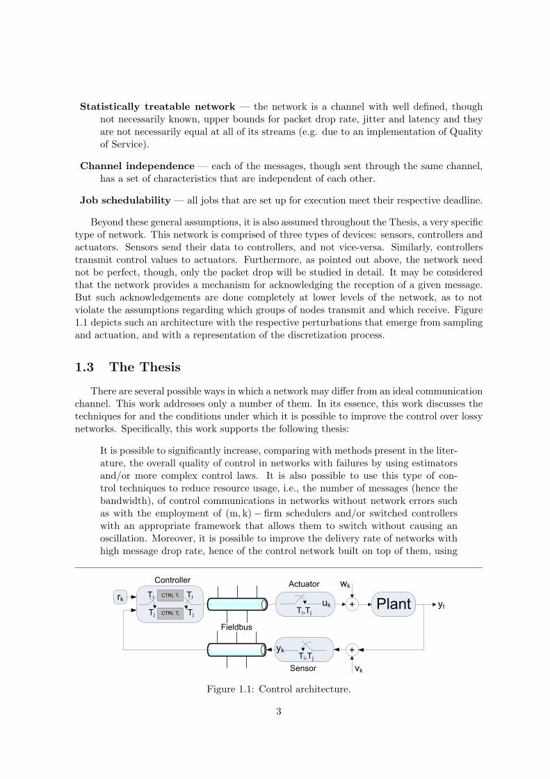
Beyond these general assumptions, it is also assumed throughout the Thesis, a very specifictype of network. This network is comprised of three types of devices: sensors, controllers andactuators. Sensors send their data to controllers, and not vice-versa. Similarly, controllerstransmit control values to actuators. Furthermore, as pointed out above, the network neednot be perfect, though, only the packet drop will be studied in detail. It may be consideredthat the network provides a mechanism for acknowledging the reception of a given message.But such acknowledgements are done completely at lower levels of the network, as to notviolate the assumptions regarding which groups of nodes transmit and which receive. Figure1.1 depicts such an architecture with the respective perturbations that emerge from samplingand actuation, and with a representation of the discretization process.

1.3 The Thesis

There are several possible ways in which a network may differ from an ideal communicationchannel. This work addresses only a number of them. In its essence, this work discusses thetechniques for and the conditions under which it is possible to improve the control over lossynetworks. Specifically, this work supports the following thesis:

It is possible to significantly increase, comparing with methods present in the liter-ature, the overall quality of control in networks with failures by using estimatorsand/or more complex control laws. It is also possible to use this type of con-trol techniques to reduce resource usage, i.e., the number of messages (hence thebandwidth), of control communications in networks without network errors suchas with the employment of (m, k)− firm schedulers and/or switched controllerswith an appropriate framework that allows them to switch without causing anoscillation. Moreover, it is possible to improve the delivery rate of networks withhigh message drop rate, hence of the control network built on top of them, using

Plantrk

Ti,Tjyk

wk

vk

yt

CTRL Ti

CTRL TjTi,Tj

ukTj

Ti Ti

Tj+

+

Controller

Fieldbus

Actuator

Sensor

Figure 1.1: Control architecture.

3

a combination of multi-path routing and algorithms that allow to reconstruct thedata with a low number of message exchanges.

The results of the Thesis are established using a variety of methods. Some of the parts ofthe Thesis are proven on purely mathematical grounds and then tested to assert their validityin practical settings. Other parts are postulated and then showed to be true (proven right)with a lower degree of mathematical abstraction. Furthermore, the Thesis is established byproving a number of intersecting lines regarding control over communication networks withpacket losses.

One such line is the use of estimators. This Thesis will provide the basic conditionson which the use of estimators can result into a lower bandwidth consumption. Furthermore,it shows that it is possible to change the actuation rate without changing the samplingrate and vice-versa. This is crucial because provided that the sampling is done at a ratethat allows for the correct estimation, then the quality of control can still be increased byincreasing the control rate. This has some far reaching implications, such as the fact that thenumber of messages among the various devices in a distributed control system can be reducedwhile maintaining the quality of control for as long as it is found a mechanism to generate atthe actuator the new control values (which are also provided in this work).

The Thesis proves empirically that the use of estimators in the controller of a distributedcontrol system can improve substantially the quality of control. The Thesis also establishesmathematically the optimal control law in networks with failures in a particular typeof output strategy. This new control is extended in a way that it produces the classical controllaws as well as the control law of another output strategy, which is present in the literature.This extension produces a new parameter which when minimized yields a controller that pro-duced output values that are similar to the values produces by the use of estimators, therebyboth proving mathematical optimality of the use of estimators and proving the existence of aduality between the use of estimators in the controller and the introduced parameterin the output.

The Thesis will also discuss aspects related with the certainty equivalence principle ofcontrol in networks with failures, thereby setting boundaries to the amount of knowledgethat can be extracted from the current control framework while giving directions into apossible way of creating an optimal controller for more restricted situations.

The possibility of using controllers in error laden scenarios brings back the possibility ofusing (m,k)-firm schedulers (schedulers in which at leastmmessages out of any consecutivegroup of k messages are successfully scheduled), or at least to model the successful deliveryof control messages as an (m,k)-firm process. In this aspect, the contribution of this Thesis istwo fold: first a new (m,k)-firm scheduler was devised that 1) provides harder guaranteesand 2) achieves a higher cpu/network utilization, and second the introduction of theoptimal scheduler gives the first steps in the direction of proposing an optimal control lawfor this type of scenarios.

The resource optimization normally requires the use of multiple controllers, each onetuned for a given scenario, which are switched as the condition of the overall control networkchanges. However, this normally introduces an oscillation in the output. This Thesis pro-vides a mechanism, which is both mathematically and simulation wise proven, to guaranteeoscillations free controller change.

At last, a mechanism that introduces and makes an efficient exploitation of pathredundancy on multi hop communication networks is also presented. Such mechanism

4

has a potential to simplify the use of controllers in communication networks composed ofseveral hops.

1.4 Structure of the Dissertation

The remaining of the Dissertation is organized as follows: the first part of this Disserta-tion deals with basic and introductory concepts. These concepts will be fundamental atestablishing the nature of the contribution that is presented in the following chapters. Thefirst part of the document has two chapters (not including the present chapter), one coveringcontrol related topics and another covering topics in network and real-time scheduling. Thesecond part of this document deals with the Dissertation per se. All chapters in the secondpart of this document include an initial state-of-the-art of the topic in question as well assome form of validation at their respective ends.

The first part of this document is organized as follows:

Chapter 1 is this chapter, which provides an overview of this document and presents theThesis.

Chapter 2 starts with an introduction to control and ends with a survey of topics in moderncontrol.

Chapter 3 provides an overview of topics related to modern real-time systems and networks.

The second part of this document is organized as follows:

Chapter 4 deals with the use of estimators for the reduction of control bandwidth.

Chapter 5 deals with the control over lossy networks.

Chapter 6 deals with control systems with multiple controllers in which the change ofcontrollers cause an output oscillation. A solution for this problem is presented andvalidated.

Chapter 7 deals with (m, k)− firm systems. More specifically, the creation of a determinis-tic (m,k)-firm scheduler that can successfully fulfill all of its (requirements) properties,which is motivated by the fact that none of the schedulers found in the literature hadall the properties sought for.

Chapter 8 presents a novel way to increase the probability of a value of a given node in awireless sensor network reach the (or a, according to the case) node that communicateswith the external network.

1.5 Contributions of this Thesis

The specific contributions of this Thesis are:

Use of buffers and estimators for bandwidth reduction— this mechanism is similar tothe send-on-delta mechanism, in the sense that the various transmissions are triggered bycrossings of some thresholds, but it differs from it because 1) the transmission thresholdsare set on the state variable as opposed to the traditional input and/or output, 2) the

5

outputs are not set to constants but they vary in a way very similar to the way theoutputs would vary if all messages were received and 3) the controller constructs animage of the system with a number of message exchange as low as possible.

Use of buffers and estimators to mitigate the effects of packet loss — this mech-anism allows the actuator to have a reasonable estimation of the output value in theperiods in which it does not receive any message from the controller. A similar effecttakes place in the sensor to controller communication.

Analytical solution for the control over lossy networks with the hold strategy —this solution allows for an optimal application of this type of output strategy

Analytical extension for linear output types — a general optimal control over lossynetworks in which the output is equal to the previous output times a multiplying matrixis given. Furthermore, the optimal value of the multiplying matrix itself is also derived.In doing so, it is proven that such generalized control is similar to the control usingbuffers and estimators, without the need for the transmission of the extra messages.Other differences are presented which help in the quantification of the effects of thetransmission of control values.

Analytical solution for the problem of oscillation free controller change — thissolved the dilemma that appears due to controller change causing oscillations thatnegated the gains of the controller change. The method is based on a change of basismatrix that is used to compute a novel state value at the switching time.

A novel deterministic (m,k)-firm scheduler — past(m,k)-firm schedulers were eitherstochastic, which guarantee the (m,k)-firm constraint in a stochastic manner, or weredeterministic.

Multipath aggregation of duplicate sensitive summaries on WSN — this contri-bution addresses the problem that arise when aggregating values from different paths.It is solved by 1) finding an algorithm to break down the various aggregates and itsays to each node which aggregate it should be sent and 2) a reconstruction algorithmthat allows for nodes to make an aggregation that dismisses duplicates and is the bestpossible in the absence of a given message or set of messages.

1.5.1 List of Publications

• Milton Armando Cunguara, Tomas Oliveira e Silva, Paulo Bacelar Reis Pedreiras:“On oscillation free controller changes. Systems & Control Letters”, 62(3): 262–268(2013). Journal.

• Milton Armando Cunguara, Tomas Antonio Mendes Oliveira e Silva, Paulo BacelarReis Pedreiras: “On the control of lossy networks with hold strategy”. SIES 2013: 290–298, Porto, Portugal.

• Milton Armando Cunguara, Tomas Oliveira e Silva, Paulo Bacelar Reis Pedreiras:“Optimal control in the presence of state uncertainty”. ETFA 2012: 1-4, Krakow,Poland

6

• Milton Armando Cunguara, Tomas Antonio Mendes Oliveira e Silva, Paulo BacelarReis Pedreiras: “A loosely coupled architecture for networked control systems”, IEEEInternational Conference on Industrial Informatics - INDIN , Lisbon, 2011.

• Milton Armando Cunguara, Tomas Oliveira Silva, Paulo Pedreiras: “On Multi-PathAggregation of Duplicate-Sensitive Functions”. 12 Conferncia sobre Redes de Computa-dores (CRC’ 2012), November 15–16, 2012, Aveiro, Portugal.

• Milton Armando Cunguara, Tomas Silva and Paulo Pedreiras: “Multipath DataAggregation on WSN ”, Workshop on Signal Processing Advances in Sensor Networks,in conjunction with the CPSWEEK’13, Philadelphia, PA, USA. April 8 2013;

• Milton Armando Cunguara, Tomas Oliveira e Silva, Paulo Pedreiras: “A Path toOscillation Free Controller Changes”, 9th IEEE International Workshop on FactoryCommunication Systems (WFCS’ 2012), May 21–24, 2012, Lemgo/Detmold, Germany.

7

Chapter 2

Background

If I have seen further it is by standing on the shoulders of giants.— Isaac Newton

This chapter presents a number of basic concepts that are paramount to fully understandthe contributions that are made in the subsequent chapters. In a sense it sets the stage inwhich the Thesis will be played. The organization of this chapter reflects the organizationof the Thesis which was put forward at the end of the previous chapter. Before entering themore advanced aspects of each subject, it is given a brief didactic introduction.

2.1 Principles of System Representation

For as long as the human species is capable of reasoning there is a necessity to thinkabout the various aspects of life. All of them require that the thinking individual engages in aseries of manipulations done over an internal representation of the object of thought. (In thiscontext, internal refers to the fact that the thinking individual manipulates its representationsand not the object that it is being represented).

In automatic control there is also a necessity to represent the various systems in a mannerthat is amenable to manipulations both by control designers as well as by the devices that willultimately implement the control in question. Such representation is usually called SystemRepresentation and it is upon it that all of the control theory is developed.

In essence, a system representation is a mapping between a set of characteristic of theobject being mapped and a series of characteristics of the objects that reside inside thethinking entity. This mapping is not always a bijection, i.e., a one to one correspondence,since only a finite set of characteristics (usually those of interest) may be mapped, but it isan endomorphism, which can be understood as being composed of two steps. The first is abijective representation in which all aspects of the world are mapped. The second step whichis applied to the intermediate mapping, removes all the aspects that are irrelevant to theentity that requires the mapping. Hence, it is an endomorphism because the representationdoes not have all the characteristics of the original system — endomorphisms are relationsthat stem from a given set to one of its proper subsets, or relations in which the codomain iscontained in the domain. Moreover, each of the possible internal states of the thinking entitythat is used to represent the system is called an image of the system.

The representations used in control systems are internal because changes in the represen-tations do not (automatically) change the conditions of the systems. In fact, to modify their

9

surroundings, the controllers use devices called actuators. Similarly, due to the internalnature of such representation, the fact that a control system has a given representation of itssurroundings does not cause its surroundings to be in that particular state. Hence there isa need to probe the environment to discover the values of such variables. The devices usedto perform this task are called sensors. This notion is fundamental in control systems ingeneral, but is more so in the context of this Thesis since the Thesis is about systems inwhich the actuator may or may not produce an output as well as the sensor may or may notproduce a reading.

It is important to stress the difference between sensing and observing, in the context ofautomatic control. Sensing is related to the acquisition of a value associated to a particularvariable, whereas observing is related to the acquisition of an image of a variable, in manycases by inference. Obviously, all aspects of a given system that can be sensed are observable,but the converse is not necessarily true. A similar relation exists between actuation andcontrol.

An entity that controls a system, henceforth a controller, that cannot cause an influence,i.e., actuate, on the system that it is supposed to control or that cannot sense a system that itis supposed to observe is not of much use. It would simply perform a series of computation onits representations without any form of interaction with the physical world. The general effectof the network errors is a reduction of the coupling between both the internal representation(through sensing) and the desired physical state (through control) with the actual state ofthe physical world. This effect is one of the main object of study of this Thesis.

Even though a proper representation of the system to be controlled is essential to asuccessful control, as discussed above, it should be stressed that from the physical point-of-view, the controller is simply another element that receives a set of sensor readings and outputsa set of actuator values. Hence, for as long as the controller outputs the values that drivethe system into the desired state, the controller’s internal representations become irrelevant.Evidently, this last observation significantly relaxes the requirements of a representation.

2.1.1 Linearity

The physical world can be thought of as being made of a series of smaller subsystems.Each one of these subsystems obey a set of mathematical rules, of varying complexity, whichare normally stated as equations. Due to such complexity, it is common to use simplifiedversions of these equations. A simplified version, or an approximation, produces results thatare qualitatively similar but quantitatively inferior to the ones produced by the non-simplifiedequation. However, they have the benefits of simplicity, namely: ease of implementation froma computationally standpoint, ease of deduction, lower processing time, among others.

Evidently, this drive to simplicity makes the simplest systems the most used ones. Oneof the simplest types of systems, if not the simplest, are the linear ones. A system is said tobe linear if it verifies the following two conditions:

Homogeneity A system is said to be homogeneous if it responds to the stimulus u(t) withy(t) then it also responds to the stimulus αu(t) with αy(t), ∀α ∈ C.

Superposition A system is said to obey the principle of superposition if it responds to thestimuli u1(t) and u2(t) with the stimuli y1(t) and y2(t) respectively, then it responds tothe stimulus u1(t) + u2(t) with the stimulus y1(t) + y2(t).

10

In general a system is linear if it is possible to write its output in the form

y(t) = H [u(t)] (2.1a)

= Ku(t) (2.1b)

in which u(t) is the input signal of the system, H is an operator that acts in signal u(t) toproduce another signal, y(t) is the output signal and K is a factor that does not depend onu(t).

If, in addition to these two properties, the system’s response does not depend on theinstant in which the stimuli are applied then it is said to be Linear Time Invariant (LTI).

Continuous-Time Representations

Due to the continuous nature at the scales normally used in control theory (i.e., ignoringquantum mechanical effects) the physical world is more readily described as a continuous-timesystem.

Continuous-time representations are characterized by the fact that the variable that rep-resents time can take any real value. In practice, this range is limited by the time of interest(duration of the experiment, simulation, etc.) which sets lower and upper bounds. Nonethe-less, the time variable is not constrained in the values that it can have in between.

Physical systems not only vary continuously in the time dimension, they also vary contin-uously in the amplitude of their respective variables. The rate of variation of a given variable,physical or otherwise, with the passage of time, in the Liebniz notation, is given by

d

dtf(t) = lim

∆t→0

f(t+∆t)− f(t)

∆t(2.2)

which is the first derivative of the function f(t). Higher order derivatives are denoted dk

dtkf(t)

with k the order of the derivative. In this Thesis only integer derivatives will be consideredwith the 0th order derivative being the function itself and the negative order correspondingto multiple integrals, though, in general, such integrals seldom appear because the respectiveequations that give rise to them are rewritten by taking derivatives of an order that make allthe integrals vanish. Continuous-time linear systems of this subclass, i.e., finite order with nodelays and integral order derivatives only, have the general form

NB∑j=0

βjdj

dtju(t) =

NA∑i=0

αidi

dtiy(t) (2.3)

in which NA and NB are finite, non-negative integer numbers characteristic of each system.Note that this equation can describe both Single-Input Single-Output (SISO) systems, ifthe respective coefficients are scalars or it can represent a Multiple-Input Multiple-Output(MIMO), if the respective coefficients are matrices.

Consider the definition of a new operator

pdef=

d

dt(2.4)

which allows Equation (2.3) to be written as

NB∑j=0

βjpju(t) =

NA∑i=0

αipiy(t) (2.5)

11

in which u(t) and y(t) can be removed from inside the summation sign. This fact, in turn,induce the definition of two new polynomials, namely

B(p) =

NB∑j=0

βjpj (2.6a)

A(p) =

NA∑i=0

αipi (2.6b)

which further simplifies Equation (2.3) into

A(p)y(t) = B(p)u(t). (2.7)

In most situations, it is assumed that A(p) and B(p) are co-prime polynomials, i.e., theyhave no common factors, since models with co-prime polynomials can be simplified into modelswithout common factors that produce exactly the same input-output response, for example,by deconvolution of both polynomials by the common term. Furthermore, it is assumed (ifnot, then normalization is carried out) that the polynomial A(p) is monic, i.e., the termassociated with the highest order of p is 1 (αNA

= 1). However, this assumption is challengedin situations in which there is another exogenous variable (i.e., a variable that affects thesystem but that is not one of the sensed inputs) in the system. In fact, the presence of anexogenous variable leads the description into

A(p)y(t) = B(p)u(t) + C(p)e(t) (2.8)

in which e(t) is the exogenous variable and C(t) is the differential polynomial associated to it.Note that the introduction of an exogenous variable changes the mutually prime assumptionstated above into: it is assumed that A(p), B(p) and C(p) are mutually prime polynomials,for the same reasons as in above.

The orders of these polynomials (A(p), B(p) and C(t)), namely NA, NB and NC are notnecessarily finite. However, in general, when they are not finite, it is still possible to approxi-mate the polynomial, using Taylor function expansions into a number of other functions. Themost common ones include the exponential (which corresponds to a (time) delay of the signalin question) and fractional derivatives. Nevertheless, in this Thesis it is assumed that NA,NB and NC are all finite.

Moreover, it is also assumed that NA ≥ NB, NC , ensuring causality. In systems in whichthis condition is not verified, a response can temporal precede its cause. A system is said tobe causal if, and only if, its responses always temporally succeed the inputs that cause them.

A given value pp is said to be a system pole if B(pp) = 0, i.e., if it nullifies the polynomialassociated with the input. Similarly, a given value pz is said to be a system zero is A(pz) = 0,i.e., if it nullifies the polynomial associated with the output. More advanced aspects ofrepresentation of linear systems, such as delays, can be consulted, for example, in [CF03].

Discrete-Time Representations

Despite the continuous-time behavior of the physical world in general, there are a numberof processes that are discrete in nature, for example the chess moves. These systems are alsolinear but are characterized by the fact that the time variable can only take a predefined setof values.

12

Discrete-time systems have a representation that is similar to the continuous-time repre-sentation, namely

A(q)y(k) = B(q)u(k) + C(q)e(k) (2.9)

in which k is the discrete-time variable, u(k) is the input signal, e(k) is the exogenous signal,y(k) is the output signal, q is the forward operator, i.e., qx(k) = x(k + 1), and A(q), B(q)and C(q) are polynomials of degrees NA, NB and NC in the variable q defined as

A(q) =

NA∑i=0

αiq−i (2.10a)

B(q) =

NB∑i=0

βiq−i (2.10b)

C(q) =

NC∑i=0

ςiq−i. (2.10c)

Note that none of the polynomials has a term with a positive exponent of q, which is dueto causality requirements. Note also that αi,βi and ςi are not necessarily equal to theircontinuous-time counterparts, such those that emerge from Equation (2.8). Advanced top-ics, regarding the representation of discrete-time systems, can be consulted, for example, in[HRS07].

Test Signals

The linearity (homogeneity and superposition) property of the systems implies that if agiven signal u(t) produces an output y(t) then H(p)u(t) (with H(p) a linear filter) producesan output equal to H(p)y(t). This fact implies that the response of any other signal can beeasily computed once the response for a well defined signal is known.

The signal best suited for serving as the basic input (test) signal is called an (unitary)impulse distribution and it can be defined, for example, by the following limits

δ(t) = limA→∞

A · rect(

t

A

)(2.11a)

δ(t) = limσ→0N (0, σ) (2.11b)

in which rect(t) is the rectangle function defined as

rect(t) =

0 if |2t| > 11 if |2t| < 112 if |2t| = 1

. (2.12)

and N (x, σ) is the Normal distribution. The former definition has the advantage of beingreadily intelligible whereas the latter definition has the advantage of being infinitely differen-tiable. Nevertheless, the impulse can be defined as the limit of any other function in whichthe limit in question has unity area and is zero everywhere except at the origin. The impulseis related to the integral operator by the relation∫

f(t)δ(n) (τ − t) dt = f (n) (τ) (2.13)

13

where (·)(n) denotes the nth repetitive derivative. Equation (2.13) is a very important property

of the impulse because it implies that (h(t)def= H [δ(t)])

H [u(t)] = H

[∫u(τ)δ (t− τ) dτ

](2.14a)

=

∫u(τ)H [δ (t− τ)] dτ (2.14b)

=

∫u(τ)h (t− τ) dτ (2.14c)

= u(t) ∗ h(t) (2.14d)

Equation (2.14a) follows directly from Equation (2.13) and Equation (2.14b) follows fromthe linearity of the integral, though there are some degenerate linear transformations that dorespect this equality. However, these transformations either seldom appear in control practiceor can be replace by a sequence of operators that do respect it, i.e., a work around, thus, suchcases are outside of the scope of this Thesis. Equation (2.14c) follows from the definition ofh(t). Equation (2.14d) defines an operator called convolution. Equation (2.14) states thatthe response of a system to a given signal is equal to the convolution of the signal in questionwith the impulse response of the system.

Equation (2.14) can be rewritten as

H [u(t)] = H(p)u(t), (2.15)

where H(p)def= A(p)

B(p) has the property that A(p)δ(t) = B(p)h(t). However, due to the super-position principle, the output of the system is also dependent of the initial values and of otherinput signals.

There are other test signals, some of them related with the impulse by the simple formulapnu(t) = δ. The simplest of such signals are the unitary (Heaviside) step, the unitary rampand unitary parabola for n = 1, 2, 3 respectively, i.e.

u(t) =

tn

n! if t ≥ 00 if t < 0

(2.16)

There are other less common test signals such as the (complex) exponentials which havea high importance for describing systems according to their frequency response. Such signalsare not used enough times within this work to deserve an in depth description. Furthermore,such signals are test signals in the sense that they are used to (physically) test the responseof systems and not to describe the properties of the systems based on the response to thesesignals.

Similarly to the continuous-time, it is possible to define a discrete-time impulse, i.e.

δ(k) =

0 if k = 01 if k = 0

. (2.17)

The discrete-time impulse has properties of the continuous-time impulse, starting with

∞∑κ=−∞

f(κ)δ (k − κ) = f (k) , (2.18)

14

which, using arguments similar to the continuous-time case, can be proven that

H [u(k)] =

∞∑κ=−∞

u(κ)h(k − κ) (2.19a)

= u(k) ∗ h(k). (2.19b)

It is also possible to define a discrete-time unitary family of signals associated with theimpulse and it is done so according to the formula (1− q−1)nu(k) = δ(k). The first three ele-ments of this family are the discrete-time unitary (Heaviside) step, the unitary ramp and theunitary parabola, for n = 1, 2, 3 respectively. Similarly it is possible to define the (complex)exponentials and other test signals discrete-time domain.

A comprehensive analysis of test signals, both in continuous-time as in discrete-time, isprovided in [CF03].

2.1.2 Discretization

As stated in previous subsection, at the scales relevant for contemporary control prac-tice, most natural phenomena are continuous-time in nature. Nonetheless, in the previousdecades there have been an explosion in microprocessor’s price-performance ratios, which ledto their wide spread adoption. Since microprocessors are discrete-time computational devices,it created a need to obtain a discrete representation of continuous-time processes.

The (uniform) discretization of a signal consists in defining a second signal

sd(k) = sc(kTs + φ), (2.20)

with sc the continuous-time signal, sd the discrete-time signal, k the discrete-time variablewhich represents the sample sequence number, Ts the sampling period and φ a phase in thesampling time which normally is equal to zero. Under certain conditions, i.e., if it appearsdue to a delay between an action and a response, φ is called dead time. Note that beside itsapplication to denote the time difference between the instant in which a value is in the outputto the instant in which it is discretized — i.e., sampling time, the term dead-time is also usedto denote the time between the application of a given control value and the appearance of itsresponse in the output.

This process is similar to the sampling process described by the Nyquist/Shannon samplingtheorem which requires the sampling frequency (defined as FsTs = 1) to be at least twice thehighest frequency contained in the signal Fourier Transform. However, the type of signals thatusually appear on control systems include signals for which there is no frequency for whichthey become zero. In fact, all forms of reconstruction are based on the system’s input/outputresponse plus the knowledge of the value of the signal in a number of (discrete) points. Thisfact renders the Nyquist/Shannon sampling theorem of little use.

Output Signal “Analogization”

In digital systems there is a need to apply the discrete-time input signal into the physicalworld. Assuming that linearity is preserved (using the arguments presented above), any suchoutput of the input signal can be produced by applying a static value, equal to the discrete-time input value at the beginning, into an analog filter for the duration of a period, whichimplies that

A(p)y(t) = B(p)O(p)us(k), kTs + φ < t ≤ (k + 1)Ts + φ (2.21)

15

with some boundary conditions on y(kTs + φ).O(p), in essence, defines interpolating values for us. Choices of O(p) are limited by the

amount of electronic instrumentation that can be used, which in turn is limited by anotherset of factors, such as, price, size of the marginal performance gain of using more electronics,desired level of integration, i.e., total component size, etc. However, due to their low-costand simplicity, a family of output filters have gained prominence, namely the nth order hold,which are defined as

(pTs)n+1O(p) =

(1− e−pTs

)n+1, (2.22)

which implies that the signal at the input of the continuous-time system is

u(t) = us(k−1)+(t− (kTs + φ)

Ts

)n+1

(us(k)− us(k − 1)) , kTs+φ < t ≤ (k+1)Ts+φ. (2.23)

The last equation is called the backward or causal version, because it uses information re-garding a sample from the past (us(k−1)). There is a similar approach that employs samplesfrom the future us(k + 1) and is called forward nth order hold and is in essence the pastequation forwarded by one sample.

The most used order is zero (order hold). This choice appears to be too simplistic to beuseful. However, its simplicity is the main reason why it reached such a wide adoption, i.e.,it only requires that a value is maintained constant for a given amount of time. The otherreason is that the flaws associated to its simplicity can be overcome by sampling the system atperiod shorter than the minimum necessary, also called oversampling, which is made possibleby the ever increasing capacity of microprocessors.

The process of generating a continuous-time signal from a discrete-time signal is calledDigital-to-Analog Conversion.

Derivative Approximations

The most simple approximations of the derivative operator are called forward and back-ward Euler operators and they discretize the continuous-time representation by approximatingthe derivative operator by a (linear) function of the delay operator. The approximations are

p ≃ 1− q−1

Ts(2.24a)

p ≃ q − 1

Ts(2.24b)

with Equation (2.24a) corresponding to the backward (computed using a previous sample)Euler approximation and (2.24b) corresponding to the forward (computed using a futuresample) Euler approximation.

With these transformations, and assuming that the pn is approximated by applying thederivative approximation n times, then, the system defined in Equation (2.7) is discretizedinto

A

(1− q−1

Ts

)y(kTs) = B

(1− q−1

Ts

)u(kTs) (2.25a)

A

(q − 1

Ts

)y(kTs) = B

(q − 1

Ts

)u(kTs) (2.25b)

16

according to the backward and the forward Euler approximations respectively.

Another approach is to use the average of these two values to produce an Euler meanmethod, i.e.

p ≃ q − q−1

2Ts(2.26)

It can be proven that this approximation is equal to the Tustin, also called Trapezoidalor Bilinear approximation (see Equation (2.27)) in the sense that their transformations ofcontinuous-time models into discrete-time models are always equal. The last statement canbe proven by considering the approximation of the inverse of the derivative (the integral oper-ator), i.e., the Euler mean approximation is the average of the approximation of the derivativeof the two Euler approximations, whereas in the Tustin case the inverse of the derivative ap-proximation is equal to the mean of the inverse of the Euler approximations. Despite bothmean Euler and the Tustin approximations produce discrete-time approximations that havethe same square error quality, they do not produce the same values of the y(t), with themean Euler assuming a constant value between two samples and the Tustin approximationassuming that y(t) varies linearly between y(kTs) and y((k + 1)Ts).

p ≃1 + q Ts

2

1− q Ts2

(2.27)

Another important aspect regarding these approximations concerns their respective sta-bility. In fact, it can be proven that the discretization of systems using the forward Eulerapproximation does not preserve stability in the sense that there are stable continuous-timesystems that are transformed by the forward Euler approximation into unstable discrete-timesystem. In the same line, both the backward Euler and the Tustin approximations pre-serve stability. However, in the inverse transformation, i.e., the transformation that turns thediscrete-time approximation into the continuous-time system that originated it, the backwardEuler is the only one that does not maintain stability. Therefore, of the three, the Tustin ap-proximation is the only one that maintains stability in both cases, hence it is the most naturalchoice for an approximation, among the considered options, from a stability viewpoint.

A related issue is the quality of the approximation. It can be proven, for example, byperforming a Taylor expansion of the systems response plus the fact that q = exp(pTs), thatthe two basic Euler approaches produce an error term of the orders greater than Ts whereasthe Tustin approximation produces errors of orders greater than T 2

s , which is another aspectin which the latter approximation is superior.

Regarding the positions of the singularities, i.e., zeros and poles, in all three cases theyare transformed according to the respective (transformation) approximation. However, theTustin approximation introduces a new set of zeros in q = −1 with a multiplicity that makesthe numerator and the denominator have the same order. One consequence of this fact is thatin all such approximations, the poles and (some) zeros tend to the point q = 1. This causessome poles and zeros to have similar values, hence some poles and zeros approximately canceleach other, which in turn requires a microprocessor with higher bit precision.

A different approach to discretization is the impulse invariant method. The impulseinvariant discrete-time system is defined as the discrete-time system to which a discrete-timeimpulse produces the same output as the discretized continuous-time impulse response. Underthis approach, the continuous-time system can be written as (assuming that B(q) has no pole

17

with multiplicity higher than one)

A(p)

B(p)=

NB−1∑i=0

γip− pi

(2.28)

which coincides with its respective impulse response. The discretization of the signal givenby the last equation is then

Ad(p)

Bd(p)=

NB−1∑i=0

qTsγiq − epiTs

(2.29)

which implies that the continuous-time poles are transformed according to qi = exp(piTs)whereas the zeros are transformed in a rather more complex manner. However, as Ts → 0,qi → 1 and it can be proven that as Ts → 0, NA zeros of the system tend to one.

The remaining NB −NA (which is positive due to causality assumptions, furthermore isan integer if the system is rational) zeros tend to a different limit. In fact, as the zeros andpoles tend to q = 1, an excess of poles (once more, due to causality assumptions) appear atq = 1. Then at this point the system behaves as if it was given by (with n = NB −NA)

A(p)

B(p)=

1

pn

which has an impulse response of:

Ad(p)

Bd(p)=

1

n!

∞∑k=0

(Tsk)n (2.30a)

= Tns

(1− q−1)n

n!(1− q−1)n

∞∑k=0

kn (2.30b)

=Tns

n!(1− q−1)n

∞∑k=0

n∑j=0

(−1)j(n

j

)q−jkn (2.30c)

=Tns

n!(1− q−1)n

n∑j=0

n∑k=0

(−1)j(n

j

)q−jkn (2.30d)

=Tns

n!(1− q−1)n

n∑j=0

j∑k=0

(−1)j(n

j

)q−jkn (2.30e)

=Tns

n!(1− q−1)n

n∑j=0

j∑k=0

(−1)j(n

j

)q−j(j − k)n (2.30f)

the first equality stems from the discretization of the impulse response of 1pn which is tn−1

(n−1)! .

The second equality is a simple multiplication (and division) by the known denominatorinferred from the known multiple poles at q = 1. The third equality follows the application ofthe binomial theorem. The fourth equality stems from the fact that

∑nj=0(−1)j

(nj

)(x−j)i = 0

for any x ∈ C, i ∈ N. This statement can be easily proven by induction. In fact, the lastproposition implies that all partial sums should be zero, however, the impulse response of thesystem is zero for values of k (time variable) lower than zero, which breaks the symmetry and

18

allows the first terms of the partial sum to not be zero because they do not yet satisfy theabove proposition. The fifth equality follows due to the fact delays of j samples are identicallyzero for the first j − 1 terms of any causal system. The last equality follows by a reorderingof the summation in k, i.e., from the end to the start.

The last equation completely defines the polynomial associated with the remaining zeros.There is the possibility to make step invariant or of higher order discretizations which basicallyconsists of 1) defining the response of the system to the signal in question, 2) discretize theresponse signal, 3) finding the equivalent discrete model and finally 4) compensate for theinput signal, i.e., finding a discrete system that when excited by the discrete version of theexcitation signal generates the discretized output signal. However, regardless of the inputsignal, the over-sampling singularity clustering effect does not disappear.

An extensive discussion on the topics on the passage from the discrete-time domain to thecontinuous-time domain and vice-versa can be found in [Lev96].

2.1.3 Stability

There are many possible definitions of Stability. In fact, the word stable has a popularassociation with finiteness. However, there are problems with this definition, since any nonidentically zero linear (and most non-linear) system(s) can be made (in theory) to producean infinity response by exciting them with a signal of infinite amplitude. This fact leads to amore rigid definition of stability, called Bounded-Input Bounded-Output (BIBO). Note thatthe term BIBO is applied to describe the system and not its current output, which can bemade to change by changing the input.

Nevertheless, BIBO systems are not to be confused with well behaved systems, since beingnon chaotic, i.e., responded in a easy to visualize way, is one of the requisites for stability inpopular notion of stability. In fact, a system does not have to always respond in the samemanner to the same input signal, i.e., it may be stochastic, in order to be BIBO stable. Theonly criteria a system must meet in order to be BIBO stable is that it must produce a boundedresponse for all input signals.

A signal u(t) (if continuous) or u(k) (if discrete) is said to be bounded, according to agiven norm if, and only if, there is a value M

|u(t)| ≤M, ∀t ∈ R (2.31a)

|u(k)| ≤M, ∀k ∈ Z (2.31b)

where | · | represents a suitable norm. The last equation means that a signal is bounded ifits norm is never bigger than a certain value.

In the set of continuous-time rational linear functions, a function is BIBO if and only ifall of its poles have a negative real part. For discrete-time rational functions, a function isBIBO if and only if all of its poles are inside the unity circle. This can be proven by showingthat systems that are claimed to be unstable respond to certain bounded signals, such asthe step functions, with an unbounded signal, and that the signals which are claimed to bebounded respond to bounded signals with bounded signals, provable by upper bounding theconvolution that defines the output.

A notable case is that of the so called marginally stable systems which are systems in whichthere is/are single pole(s) at the boundaries (real part of the poles equal to zero or moduloof the poles equal to one, for continuous-time and discrete-time systems, respectively). Note

19

that there may be more than one such singularities, but each and every one of them musthave multiplicity one. These systems are not BIBO because when excited by a signal that hasa pole at that exact location, they produce a signal that grows linearly (in norm-2 squared)with time, hence being unbounded. However, they meet most criteria for stability when theparticular type of signal is not introduced into the system. Systems that present this type ofbehavior are also called resonant. In fact, this term is used more broadly even for systemsthat have complex conjugate poles inside the region of convergence, but are relatively closedto the boundaries (also called under dumped).

Note, however, it is possible to excite a non BIBO system with a signal that makes itproduce a bounded output. Theoretically, this can be achieved by producing a signal with anappropriate zero (with positive real part or outside of the unit circle according to the case),in essence doing what is called a zero-pole cancelling.

A less strict test of stability (of linear non-stochastic systems), and also more used, is theRoot Mean Square (RMS) test of the impulse response, with some variants that include theso called impulse power test. If this value is zero, i.e., zero mean-power, then the system isstable. If it is finite but non-zero, then the system is marginally stable and if it is infinite,then it is unstable. The RMS of a signal is defined as, in the continuous and discrete-timerespectively as

hRMS = limT→∞

√1

T

∫ T

0|y(t)|2 dt (2.32a)

hRMS = limk→∞

√√√√1

k

k∑0

|yκ|2. (2.32b)

Note that the last test is not sensitive for continuous-time functions that contain δ(t).Further introductory topics in stability can be found in [HRS07] and [CF03].

2.2 State Space Representations

There are many books that present a comprehensive view of state space representations.For a more in-depth than the approach presented in here see [CF03] or [HRS07]. For afull presentation, see [Lev96]. The latter reference also has a comprehensive presentation ofKalman filters.

The hitherto presented polynomial representation cannot take into account all relevantaspects of a given system. An example is an unstable system which is stabilized by puttingon its input a compensator that cancels all destabilizing poles. Under such circumstances,the representations presented thus far would imply that the new system is stable. However,if there is a non-zero initial value, associated with an destabilizing pole, on the inputs of thesystems/outputs of the compensator (stemming for example by the presence of a non-fullydepleted capacitor), then the internal signal will grow unboundedly. This type of systems arecalled internally unstable.

Of course, it is possible to deal with this type of issues by using feedback or any othercontroller technique. However, from a system representation point-of-view, it shows thatthere are aspects that are not fully captured by the polynomial representation.

An alternative is the use of the so called state space representation. This representationhas two dynamic equations. The first equation, also called the update equation, encapsulates

20

all of the aspects of the system dynamics, i.e., how the state evolves with time. In spite of thenames of the respective equations, this is the only equation that has any form of dynamics.The second equation is called the output equation and it specifies how the (output) visibleaspects of the system are produced from the system state. As for the state per se it is avariable that encapsulates all the history of the system up to that point. In other words,knowing the state of a system allows to compute the value of all variables of the system thatcan be determined by knowing the history of the system up to that point.

In the continuous-time linear case the dynamic equations are given by

dx(t)

dt= Ax(t) + Bu(t) (2.33a)

y(t) = Cx(t) + Du(t), (2.33b)

where x(t), u(t) and y(t) are the state, input and output variables (signals) respectively, atinstant t. These variables are in the general case, i.e., MIMO, column vectors with dimensions(1× n), (1× q) and (1× p) respectively. A, B, C and D are the transition, input, output anddirect transmission matrices respectively with dimension (n× n), (n× q), (p× n) and (p× q)respectively.

Matrix A is responsible to transmit the signal from the current state to the next. MatrixB conveys the input into the future states. Matrix C describes how the state appears in theoutput, and matrix D conveys how the input can be/is propagated directly into the output.However, in causal systems with propagation delays — virtually all physical systems — matrixD is equal to a matrix of zeros of appropriate size, i.e., 0p×q. This notation (which will beused throughout this Thesis) means that it is a matrix with p lines and q columns in whichall entries are 0.

The state space representation is invariant to the similarity transformation, i.e., given anynon-singular, i.e., det(P) = 0, matrix P, the transformation x(t) = Px(t) does not changethe response of a system given its input. Nevertheless, the similarity transformation changesthe values of the matrices according to (due to the simplicity of the transformation no proofis given)

B = P−1B (2.34a)

A = P−1AP (2.34b)

C = CP. (2.34c)

This transformation is used in this Thesis to establish one of its results.The response of the system state to an input signal can be easily computed,

px(t) = Ax(t) + Bu(t) (2.35a)

px(t)− Ax(t) = Bu(t) (2.35b)

x(t) =(pIn − A

)−1Bu(t). (2.35c)

The output response is derived by recalling Equation (2.33b), leading to

y(t) = C(pIn − A

)−1Bu(t) + Du(t) + CeAtx(0). (2.36)

in which In is the identity matrix of size n which is a square matrix (of size n) in which thediagonal entries are comprised by 1 and the remaining entries are all equal to zero. The x(0)

21

denotes the initial state and the term in question can be proven by repeating the analysiswith an initial state and no input plus the application of the superposition principle. Thisequation proves the similarity invariance statement made before.

The last equation implies that the poles of the system are equal to the eigenvalues ofmatrix A. Therefore, continuous-time, linear time-invariant systems are BIBO stable if alleigenvalues of the matrix A have negative real part; they are marginally stable if thereare eigenvalues, with multiplicity one, with real part equal to zero and no eigenvalues withpositive real part; they are unstable if there are eigenvalues with real part equal to zero andmultiplicity higher than one or if there is at least one eigenvalue with positive real part.

It is also possible to write a discrete-time state space equation, see [HRS07] for moredetails,

x(k + 1) = Ax(k) +Bu(k) (2.37a)

y(k) = Cx(k) +Du(k), (2.37b)

in which the various variables and matrices have meaning and sizes similar to their continuous-time counterparts. As with Equation (2.36), the output response in the discrete-time is

y(k) = C (qIn −A)−1Bu(k) +Du(k) + CAkx(0). (2.38)

Unlike the other representations, in the state space one, if the intersample behavior of theinput is known, the effects of discretization can be fully taken into account, i.e., the discretizedrepresentation is not an approximation. Moreover, this Thesis focus on the discretization ofcontinuous-time systems subject to inputs with a zero order hold. Under these circumstancesand using Equation (2.36) (actually its state equivalent) with D = 0p×q and starting at timet = kTs (as opposed to t = 0), then (after solving the resulting differential equation)

x((k + 1)Ts) = eATsx(kTs) +

∫ Ts

0eA(Ts−t)dt Bu(kTs) (2.39)

in which the checked matrices (·) denote continuous-time matrices.A comparison of Equation (2.37) with Equation (2.39) implies that

A = eATs (2.40a)

B =

∫ Ts

0eA(Ts−t)dt B (2.40b)

C = C. (2.40c)

The equality of the output matrices stems from the fact that the output equation does notpossess any dynamics, hence it is not affected by the discretization process. Equations (2.40a)and (2.40b) can be rewritten as[

A B

0r×n Ir

]= exp

([A B

0r×n 0r×r

]Ts

). (2.41)

2.2.1 Static Non-Linearity

The previous section assumed that the system was LTI. However, there are some non LTIsystems in which the above theory can be extended into without significant changes. Such

22

systems have a so called static non-linearity, which means that the dynamic equation is stilllinear.

Among the static non-linear systems there are two non-disjoint subgroups: the Wienerand Hammerstein systems. The Wiener systems are characterized by a non-linearity in theinput, but a linear dynamic. This is typical in industrial systems in which the input isnormally comprised of motors with non-linear response. Such systems are normally linearizedby dividing the system input-output response into a series of segments that are approximatedby lines.

Hammerstein systems are characterized by a non-linear output sampling, i.e., the sampledvalue is a non-linear function of the state variable, but have a linear dynamic equation. Dueto advances in microcontrollers, this type of systems are less common nowadays. In fact,modern digital-to-analog converters produce samples with non-linear components that arenegligible for most applications.

Throughout this Thesis, it is assumed that the controlled system has a linear dynamics.

2.2.2 Linear Systems with Noise

Equation (2.33a) defined continuous-time (linear) system dynamics. However, it is rathercommon for physical systems to not evolve exactly as described by such equations. Sometimes due to perturbations, other times due to deficiencies of the model and most times dueto a combination of both.

Nevertheless, it is possible to write the dynamic equations using a noise vector that ac-counts for the difference between the value produced by the model and the value of thephysical system. This transforms Equation (2.33a) into

dx(t) = Ax(t)dt+ Bu(t)dt+ dw(t) (2.42)

in which w(t) is the variable that encapsulates all the aspects of the physical system thatare not taken into account by the model. The reason why the last equation looks ratherdifferent from past dynamic equations (with respect to the derivative) is that the stochasticvariable w(t) is (in general) not differentiable. The solution of such equation, which is also astochastic variable, is a stochastic integral which is one of the objects of study of the disciplineof stochastic calculus and is out of the scope of this Thesis.

A causal (non causal) noise sequence is said to be white if its previous (all other) valuescannot be used to predict the value of the current sample, i.e., in a white noise sequence, thesamples are statistically independent. A color is attributed to a noise sequence according tothe color of a filter that could potentially produce that noise sequence by filtering a whitenoise sequence. In turn, the color of a filter is the color that an optical filter, with a shapesimilar to the shape of the filter in question, would produce when illuminated with whitelight.

The auto-covariance of a given stochastic variable m is defined as

cov(m) = E[(m− E [m])(m− E [m])′

], (2.43)

in which (·′) denotes (Hermitian) transposition.

The variable w(t) is itself modelled as being a zero mean, white gaussian noise withan auto-covariance of Q. The whiteness assumption does not necessarily lead to a loss of

23

generality since under certain assumptions the w(t) could be modelled as having a dynamicgiven by

dw(t) = Aww(t)dt+ dε(t) (2.44)

and under these circumstances Equation (2.42) can be rewritten as[dx(t)

dw(t)

]=

[A In

0n×n Aw

]x(t)dt+

[B

0n×q

]u(t)dt+

[0n×n

In

]εdt, (2.45)

which is driven by the white noise ε.Regarding the gaussian noise assumption, its non-validity is irrelevant, as will be seen

below. Regarding the zero mean assumption, note that this is a standard noise assumption.Moreover, when it is not verified, it is said that there is an offset in the input which is normally(implicitly) corrected by u(t).

System Noise Discretization

As discussed in the previous section, the input noise is stochastic. The discretization ofthe input noise should aim at generating a (stochastic) discrete sequence of noise terms thatproduces an effects on the state variable, at the sampling instants, that are similar to theeffects of the continuous-time noise (at the same instants). However, the input noise is notknown which makes the generation of a discrete noise sequence rather difficult. Instead, it isassumed that there is a (stochastic) discrete sequence which is modelled as a gaussian noisewith known parameters, derived from the effects of the continuous-time input noise effects onthe state variable.

Due to the assumptions regarding w (i.e., that it is zero mean) and since the noise onlyundergoes linear operations then the discrete-time noise variable is also zero mean. Regardingits variance, according to the discussion on the previous paragraph

dw(t) = Aw(t)dt+ dw(t) (2.46a)

w(kTs) = 0n×1 (2.46b)

w(k)def= lim

ϵ→0+w(kTs − ϵ) (2.46c)

The first two lines define another noise sequence that evolves as the system noise but is reset atthe beginning of every period. The discrete-time noise is equal to the value that the auxiliarynoise sequence had right before the rest. This definition of the discrete-time noise impliesthat

E[w(k)w(k)′

]= lim

ϵ→0E[w((k + 1)Ts − |ϵ|)w((k + 1)Ts − |ϵ|)′

](2.47a)

= limϵ→0

E

[∫ (k+1)Ts−|ϵ|

kTs

eA((k+1)Ts−t)w(t)(eA((k+1)Ts−t)w(t)

)′dt

](2.47b)

=

∫ (k+1)Ts

kTs

eA((k+1)Ts−t)E[w(t)w(t)′

]eA

′((k+1)Ts−t)dt (2.47c)

=

∫ Ts

0eA(Ts−t)Qwe

A′(Ts−t)dt (2.47d)

=

∫ Ts

0eAtQwe

A′tdt (2.47e)

24

For stable systems, it is possible to rewrite

E[w(k)w(k)′

]=

∫ Ts

0eAtQwe

A′tdt (2.48a)

=

∫ ∞

0eAtQwe

A′tdt−

∫ ∞

Ts

eAtQweA

′tdt (2.48b)

=

∫ ∞

0eAtQwe

A′tdt− eATs

∫ ∞

0eAtQwe

A′tdteA

′Ts (2.48c)

= W − eATsWeA′Ts (2.48d)

in which

Wdef=

∫ ∞

0eAtQwe

A′Tsdt. (2.49)

This method only works for stable systems because otherwise the integral that definesW does not converge. For non-stable (including marginally stable) systems, the covariancematrix is computed by breaking down the integral in question and solving it for each entry.This method has the disadvantage of not using the various tools available to solve the morespecific types of equations. W itself can be computed by integrating the last equation byparts leading to

eATsW +WeA′Ts = Qw. (2.50)

Equation (2.50) is an important and recursively appearing equation in Control Theoryand it is called Continuous-Time Lyapunov equation. This equation is essential in one of thecontributions of this Thesis.

There is another type of perturbation associated with an uncertainty in the output, i.e.,sampling error. This uncertainty is in general not dynamic. However, the noise is possiblya colored sequence (for example, an Analog-to-Digital Converter used at a relatively highfrequency introduces a small correlation between its readings). If such correlations exist thenit is always possible to give this noise term a treatment similar to the treatment given tocolored input perturbation, thus rendering the output noise white.

The whiteness of the output noise implies that its covariance matrix is independent ofthe sampling period since by definition having more data regarding a white variable doesnot lead to a decrease of the variance of its estimates. In fact, a more in-depth explanationwould require the theory of Power Spectral Analysis, which is outside the scope of this Thesis.The overall effect of this sampling period independence is that it renders this perturbationeasy to discretize because by definition its mean and covariance matrices are equal to theirrespective continuous-time counterparts. Nevertheless, if the sampling device is operated ata frequency high enough as to introduce a correlation between the readings, the correlatedpart can be modelled with a state equation, leading to a discretization that has the two typesof components discussed above.

With these two new noise terms the state space discrete-time linear system is written as

x(k + 1) = Ax(k) +Bu(k) + w(k) (2.51a)

y(k) = Cx(k) + v(k), (2.51b)

with v(k) the perturbation that arises from sampling: v(k) is not a property of the systemper se, it is a property of the sampling device, though it may causally affect the system ifthere is a form of feedback in which the output is used to compute the input.

25

Without lossy of generality, it is assumed that

E

[[wj

vj

] [wk

vk

]′ ]=

[Q 0n×r

0r×n R

]δjk, (2.52)

where δjk is the Kroenecker delta, which is one if j = k and zero otherwise. This assumption(no correlation between input and output perturbations) does not cause a loss of generalitybecause it is always possible to decompose the output noise into two components, one corre-lated and another uncorrelated with the input noise respectively. Subsequently, the part ofthe output noise that is correlated with the input noise is sent into the input by removing itfrom the input and replacing it with an input noise that generates exactly the same (presentand future) outputs, even though it would generate a different state. In short, the correlatedpart is made to belong only to the state.

2.2.3 Continuous-time Kalman Filter

The noise components discussed in the previous subsection have an effect in the amountof information (as measured by a suitable norm of the state auto-covariance matrix) that isknown about the system, either due to the input noise causing an (or increasing the) uncer-tainty in future states and/or due to the output noise diminishing the amount of informationobtained by sampling.

In most cases, the predictions of a model are useful only if the predictions are related tothe physical variable that the model predicts. For this reason, whenever there is the possibilitythat the model predictions and the physical variables differ there is a need to measure andpossible correct such differences.

An usual such measure, which is used throughout this Thesis, is the square of the so callednorm-2 and is denoted

||e(t)||22 = ||x(t)− x(t)||22 (2.53a)

= E[(x(t)− x(t)) (x(t)− x(t))′

](2.53b)

however, neither e(t) nor the measure ||e(t)||2 are known. If they were known then it wouldbe possible to correct the models prediction, so that it would become 0n×1 . Hence if suchvalues were deterministic then they would be zero. This means, that they only make sensein expectation, hence a covariance matrix ||e(t)||2. A similar argument implies that theexpectation of e(t) (of a non biased) prediction error is always zero.

For the linear system in question, it implies that the dynamic equations, when appliedto the expected state (note that the dynamic stochastic equation is equal to the dynamicequation of the physical system because the system is linear) leads to

dx(t)

dt= Ax(t) + u(t) (2.54)

in which a new variable x signals the state estimation. Subtracting Equation (2.51a) fromEquation (2.54) and remembering the definition of e(k) yields,

de(t)

dt= Ae(t)− w(t). (2.55)

26

Note the presence of the minus sign in w(t). Since the value of w(t) is not known, for example,it could be +1 with a plus sign or a −1 with a minus sign, this sign is of little relevance leadingmany (to the best of the author’s knowledge, all) classical theories to ignore it and assumethat w(t) itself had the opposite sign. However, in this Thesis it will be presented a resultthat requires that w(t) to appear with different signs in the error equation and in the physicalstate equation, thus making it relevant.

Right multiplying Equation (2.55) by e(t)− w(t), which is the integral of d(e(t)− w(t)),for motives that will soon become apparent, leads to

de(t) (e(t)− w(t))′ =(Ae(t)dt− dw(t)

)(e(t)− w(t))′ (2.56a)

de(t)e′(t) = Ae(t)e′(t)dt+ dw(t)w′(t). (2.56b)

The last transformation is warranted due to the assumption that w(t) is white, moreprecisely, since e is a causal function of values of w and by the whiteness assumption, thecurrent value of w does not depend on its previous values, then e(t) and w(t) are uncorrelated.Nevertheless, once more, this assumption is general, in the sense that the state can always beaugmented in a way that it becomes true. Continuing,

de(t)e′(t) + e(t)de′(t) = Ae(t)e′(t)dt+ e(t)(Ae(t))′dt+ dw(t)w′(t) + w(t)dw′(t) (2.57a)

d(e(t)e′(t)

)= Ae(t)e′(t)dt+ e(t)e′(t)A′dt+ d

(w(t)w′(t)

)(2.57b)

dP(t) = AP(t)dt+ P(t)A′dt+ Qwdt (2.57c)

dP(t)

dt= AP(t) + P(t)A′ + Qw. (2.57d)

The first equality follows by adding its (own) transpose to Equation (2.56a). The second equal-ity follows by the product rule (in reverse) of derivatives and is the reason why d(e(t)−w(t)was chosen as a factor. The third equality follows by taking expectations and the definitions

P (t)def= E [e(t)e′(t)] and (the already presented definition of) Qw. The last equality follows

by noting that the right side of the previous equation is a multiple of dt and that the derivativeof P(t) is a well defined quantity.

The last equation is sometimes called the update (or innovation) equation because itdefines how the error is updated. Other times it is called the a prior equation because itstates what happens before a new measurement is assimilated by the model.

However, in continuous-time both the update of the covariance matrix and the receptionof a new value happen in the same time instant, which suggests that a better approximationof the physical state is

dx(t)

dt= Ax(t) + u(t) + K(t)

(y(t)− Cx(t)

)(2.58)

in which K(t) is a (time-dependent) gain matrix. The gain matrix is assumed to be lineardue to the linearity of the underlying equation. Equation (2.58) implies that the predictionerror evolves according to

∂e(t)

∂t= Ae(t)− dw(t) + K(t)

(v(t)− Ce(t)

), (2.59)

27

which when treated as Equation (2.55) (multiplied by(e(t)− w(t) + 1

2K(t)v(t))′, then added

to its own transpose, group similar terms and derive in order to t), gives

∂P(t)

∂t= AP(t) + P(t)A′ + Qw −

(K(t)CP(t) + P(t)

(K(t)C

)′)+ K(t)RK′(t). (2.60)

It is possible to choose a value of the free parameter K(t) in order to minimize P(t). Thisis achieved by differentiating the last equation in order to K(t) and equating it to zero, i.e.,

(with Rdef= E [v(t)v′(t)])

1

2

∂2trace(P(t)

)∂K(t)∂t

= −CP(t) + RK′(t) = 0p×n (2.61)

which is solved for

dP(t)

dt= AP(t) + P(t)A′ + Qw − P(t)

(K(t)C

)′(2.62a)

K(t) = P(t)C′R−1. (2.62b)

In the last equation, P(t) was taken with a total derivative. That is due to the fact that itno longer is a function of K(t), but it is a function of P(t) itself, of some covariance matricesthat for all effects and purposes are constants. Hence the only free variable is time.

Equation (2.62), which dictates the evolution of the state estimate covariance matrix, andEquation (2.58), which dictates the evolution of the state estimates, are called the Kalman-Bucy filter and they are the optimal way to filter continuous-time perturbations.

It is somewhat common to see Equation (2.62a) written as

dP(t)

dt= AP(t) + P(t)A′ + Qw − K(t)RK(t)′ (2.63)

due to the equality K(t)RK(t) = P(t)(K(t)C

)′which is easily verifiable taking into account

the definition of K(t).

2.2.4 Discrete-time Kalman Filters

Despite their names, the only Kalman filter that were proposed by Robert Kalman isthe discrete version which will be presented in this section. The continuous-time version wasintroduced by Richard Snowden Bucy, but due to the similarities with the discrete version italso carries the Kalman name.

As in the continuous-time case, Equation (2.51) defines the dynamic of the state. Andthe dynamics of the state estimation is given by

x(k + 1|k) = Ax(k|k) +Bu(k), (2.64)

in which x(i|j) denotes the estimate of the state at instant i given all the information thatwas received up to the instant j.

Equation (2.64) implies that

e(k + 1|k) = Ae(k|k)− w(k) (2.65)

28

which when multiplied by its own transpose and using the definitions of the covariance ma-

trices (P(k)def= E [e(k)e′(k)] and of Qw presented before)

P(k + 1|k) = APA′ +Qw. (2.66)

Equation (2.64) and Equation (2.66) are called the update (or innovation or a priori)equations and together they define how the state estimation and its associated covariancematrix evolve from the estimation of the previous to the current.

The notation x(m+ n|m) and P(m+ n|m) denote the state estimation at instant m+ ngiven all the information about the system available up to instant m, i.e., [u0 u1 · · ·un+m] and[y0 y1 · · · ym]. Note that the information points regarding the input goes up to m+n whereasfor the output goes only to m. For n > 0, these types of estimates are acquired by applyingn (consecutive) times the update equations over x(m|m) and P(m|m). For n < 0, this leadsto a special type of Kalman filter called Fixed-lag Smoothers.

Once x(k + 1|k) and P(k + 1|k) become known there is the problem of integrating theoutput measurement, i.e., y(k), into x and P. This can be achieved by once again assumingthat linearity is not lost, i.e.,

x(k + 1|k + 1) = x(k + 1|k) +Kk+1 (y(k + 1)−Cx(k + 1|k)) (2.67)

with a new free variable Kk+1. This choice has the added benefit of ensuring that the error isnot a function of the state variable, which is an important property in control systems. Withthis definition of x(k + 1|k + 1), the error associated with state estimation becomes

e(k + 1|k + 1) = e(k + 1|k) +Kk+1 (v(k + 1)−Ce(k + 1|k)) , (2.68)

which when right-multiplied by its own transpose and taking expectation yields

P(k+1|k+1) = (In −K(k + 1)C)P(k+1|k) (In −K(k + 1)C)′+K(k+1)RK′(k+1). (2.69)

This can be minimized with respect to K(k+1) by taking the derivative of P(k+1|k+1) inorder to K(k + 1) and equating it to zero, i.e.

dTrace (P(k + 1|k + 1))

dK′(k + 1)= (In −K(k + 1)C)P(k + 1|k)C′ +K(k + 1)R = 0n×p, (2.70)

which is solved for

K(k + 1) = P(k + 1|k)C′ (CP(k + 1|k)C′ +R)−1

(2.71)

which when substituted back into Equation (2.69) yields

P(k + 1|k + 1) = (In −K(k + 1)C)P(k + 1|k). (2.72)

Equations (2.67), (2.71) and (2.72) comprise the so-called correction step of the Kalmanfilter. They define how the prediction or update made from the previous state and the dynamicof the system is corrected by the noise outputs.

29

2.3 Control

The act of, and the need for, controlling the world is as old as the human kind itself. Ithas been the main drive behind tool building throughout millennia. However, the types ofcontrol that arise from simple interaction of the human brain (or any other animal’s) withthe world, through its senses and limbs, are far from the topics that normally appear onthe contemporary control theory, though the possibility of using this type of control is notprecluded. For example, the recent emergence of robots made questions such as the optimalityof teacup handling a control topic.

One of the most basic control entities, called a servomechanism, is an automatic deviceof the actuator family, that can maintain a certain input value (obviously, with sensing,computing and actuating capacity). Evidently, it is necessary to define the word automatic,but before this is done there are a number of other terms that need to be defined.

A transducer is defined as being any device that converts signals from one domain intoanother. Examples of such domains include the electrical, temperature, pressure, humidity,liquid levels, etc. A transducer that translates a physical quantity into a quantity that can betreated, either by humans or by machines, is called a sensor. Sensors can be further classifiedinto indicators and registers. Indicators are sensors in which their readings are used (mostlyin displays for human consumption, hence their name) and discarded, whereas registers aresensors in which readings are kept in some form. There is another group of transducers, calledactuators, which are used to transduce quantities produced either by humans or by machinesinto the physical world. Due to the electronic nature of most machines, normally sensorstransduce into the electrical domain whereas actuators transduce from the electrical domain.

A control system is said to be manual if there is a human being sensing the system,building a mental representation, using a number of rules to derive new control values, andthen applying such values to the external world. A control system is said to be automaticif the control loop is closed without human intervention. Nevertheless, there are cases inbetween. For example a human typing sensed values (through vision) into a keyboard that isconnected to a computer that computes the control values and produces the outputs. Anotherexample is that of a computer system with cameras (vision) and controllers but with limitedactuation capabilities (for example, the operation of some industry machinery). In this case,the algorithm is run by the computer but the actuation is done by human beings. Usually asystem is called manual or automatic according to who/what is doing the control, regardlessof who/what is doing the sensing and actuation.

The oldest automatic control processes on record are those of mechanical watches datingback for several centuries B.C. Other typical ancient processes that do not required humanintervention were the sacred motions within temples in which apparent lack of a reason forthe motion in question was upheld as a proof for the actions of a deity, for example, the doorsof Heron. Other early examples of automatic control systems include windmills.

However, the first control system to be designed and later analysed in a manner thatresembles modern forms of control was the Ball (or centrifugal) Governor invented by JamesWatt, and was fundamental in the development of the steam engine which fueled the in-dustrial revolution. A governor is a device intended to keep a given speed constant. In amore modern vernacular it was a non-zero regulator or a speed servomechanism. Arguablythe first publication regarding control systems theory was done by James Clerk Maxwell in1868 entitled on “On Governors” [MAX68]. The publication in question introduced somefundamental concepts that are still in use in modern control.

30

However, Control Theory remained an almost dormant field until the 1920/1930 whenthe electronics and telecommunications revolution created both a need and means to realizethe control systems. One of the most important revolutions of this time came from OliverHeaviside, which used the Fourier transform:

F (jω) = F f(t) =∫ ∞

−∞f(t)e−jωtdt (2.73a)

f(t) = F−1 F (jω) = 1

2πj

∫ ∞

−∞F (jω)ejωtdjω (2.73b)

and the (bilinear) Laplace transform

F (s) = L f(t) =∫ ∞

−∞f(t)e−stdt (2.74a)

f(t) = L−1 F (s) = 1

2πj

∫ σ+j∞

σ−j∞F (s)estds (2.74b)

in which the first equation of each group defines the transform and the second the inverse.The inverse Laplace transform must be taken for σ greater than the real part of all thesingularities of F (s).

It can be shown that the continuous-time linear rational systems, as defined in Subsec-tion 2.1.1, can be transformed into a polynomial equation in the variable s. In fact, theFourier/Laplace transform the p operator into jω/s respectively. This framework for theanalysis of Control Systems became known has the frequency domain approach.

In 1932 Harry Nyquist at Bell Labs introduced the first test of BIBO stability [Nyq32].It was a graphical method that determined the stability of feedback Control Systems with itsworking principle enrooted in the theory of complex analysis. The next landmark in ControlTheory occurred with the publication of Harold Hazen [Haz34] in 1934. Though the articledid not introduce many new and important results, it introduced important concepts such asdumping factors and time constants which are extensively used nowadays.

Harold Black made an important contribution regarding systems with linear feedback[Bla34] that nowadays is commonly taught in introductory control classes. He proved that itis possible to exchange gain for bandwidth, i.e., linear systems have a constant gain-bandwidthproduct and the value of each variable is a function of the amount of feedback.

The following landmark contribution came from Hendrik Bode that realised that therewas a relation between amplifier’s frequency response gain and phase. This fact limited therange of possible realizable systems, facilitating their analysis. In fact, Bode perfected theNyquist plots into their current form and introduced a new type of asymptotic plots thatcarry his name. Bode also introduced the concept of gain margin, i.e., the reciprocal of theamplifiers’ gain at the (first) frequency that generate a phase of 180, and phase margin, i.e.,the 180 minus the phase at the (first) frequency in which the gain is unitary. Most of Bode’swork, though extensive, were presented in one single article [Bod40].

In 1948 Walter R. Evans developed one of the most intuitive graphical methods namedRoot Locus [Eva50], in which the open loop singularities are used to derive the properties ofthe closed loop system. More concretely, it describes the path of the closed loops poles as agiven parameter of the system is changed.

31

2.3.1 Modern Control

Ironically, Modern Control emerged out of concepts that were developed at the turn ofthe last century, with the Aleksandr Lyapunov and (Jules) Henri Poincare works on stabilityof linear systems, that gave birth to the modern understanding of stability.

Lyapunov Stability and Equilibrium

Consider (non)linear systems given by the state dynamic dx(t)dt = f(x(t)) and x(0) = x0

(initial state). Consider also that there is an equilibrium point denoted xe in which the statecan be at rest (f(xe) = 0n×1).

The equilibrium is said to be Lyapunov stable if there is a region surrounding the equilib-rium point such that whenever the state enters the region, it never leaves it. Such equilibriumis said to be asymptotically stable if once a state enters this region it converges asymptot-ically to the equilibrium point. And is said to be exponentially stable if the asymptotes ofconvergence are negative exponential functions.

An useful analogy for the Lyapunov stability is that f(x) is landscape with peaks andvalleys. The equilibrium points are the valleys (peaks) such that f(x) = 0, i.e. points thatare locally horizontal. An equilibrium point is stable if it is surrounded by points that areabove it, is indifferent (in a given direction) if the height of the landscape does not change ifthe state is moved in that direction, and an equilibrium point is unstable if it is surroundedby points that are below it. It is asymptotically stable if when dropped close enough to theequilibrium point, it will end up falling into the equilibrium and exponentially stable if thefall is exponential.

Lyapunov then established that a system is stable if there is a positive definite function(called Lyapunov function) which has a negative definite time derivative that satisfies certainconditions. In certain systems finding a candidate function with this property may be non-trivial. For physical systems, the energy of the system is always a Lyapunov function, and itis interpreted as: the system is stable (in a given region) if its energy is strictly monotonicdecreasing (for non-zero value).

Remarks similar to the ones made above can be made regarding discrete-time system.

For the particular case of linear systems, the Lyapunov stability degenerates into thestability test regarding the eigenvalues (poles) of the system presented in Subsection 2.1.3.For more information into discrete-time stability criteria see [HRS07], as for the continuous-time case, consult [CF03].

Controllability and Observability

The Lyapunov analysis does not answer questions regarding the (possibility of) stabiliza-tion of unstable systems. It was limited to establishing whether a system is stable whenunforced. The principles that will be presented shortly are attributed to Robert Kalman andaddress this problem for discrete-time linear function. A continuous-time version is analogousand will not be presented.

A system is said to be fully controllable if (after a given predefined amount of time) it canbe taken from one state into any other and is called partially controllable if only a subset ofits states are controllable. It can be proven that a system is fully controllable if the matrix

C =[B AB A2B · · ·An−1B

](2.75)

32

has rank equal to n, recall that n is the number of state variables. The rank of a matrix isdefined as the number of linearly independent rows/columns.

Similarly, a system is said to be observable (discrete-time) if the matrix

O =[CCACA2 · · ·CAn−1

]′(2.76)

is full rank. By observable it is meant that it is possible to infer its current state by knowinga number of past outputs.

A system may not be fully controllable (observable). The states that contribute for thenon-controllability (non-observability) are called non-controllable (non-observable) and theremaining are called controllable (observable). This defines four types of states: controllableobservable, non-controllable observable, controllable non-observable and non-controllable non-observable. It is possible to prove that non-controllable observable states in one representationcan be transformed, through a similarity transformation, into a controllable non-observablestate in another representation. The study of non-controllable non-observable states may seemlike a futile endeavor, however, such states of a system may become controllable observableif the system in question is connected to other systems. In fact, this was one of the mainhistorical motivation to describe this types of states.

Regarding stability, a system is said to be stabilizable if all of its unstable states arecontrollable. Similarly, a system is said to be detectable if all of its unstable states areobservable.

Besides these input to state and state to output relation, it is also defined the inputto output controllability (full input observability is almost never possible). State controlla-bility does not imply output controllability and output controllability does not imply statecontrollability. A system is output controllable if and only if the matrix

M =[CB CAB CA2B · · ·CAn−1B

](2.77)

has rank n.These concept are explored in more detail in [CF03] and [Lev96].

Pole placement

Pole placement is a control (observer) technique that uses a feedback matrix to positionthe closed loop poles at any location of the root locus. Though, this technique has a numberof limitations, namely, 1) the number of poles does not change, 2) the energy necessary forposition the poles at regions may be restrictive, and 3) the position of the zeros is unchanged.

In pole placement and in many of its successor techniques, the position of the controller andobserver poles can be set independently. This allows to perform the two processes separately.The control (observer) equations are given by (respectively)

u(k) = −Kctrlx(k) (2.78a)

x(k + 1) = Ax(k) +Bu(k) +Kobs (y − Cx(k)) . (2.78b)

A possible solution for SISO systems is called the Ackerman formula and is equal to

Kctrl =[01×(n−1)1

]C−1p(A) (2.79a)

p(λ) =

n−1∏i=0

(λ− λi) , (2.79b)

33

in which λi are the desired poles. A similar mechanism exists for the observer gain, which canbe found by commuting B ↔ C′ and A ↔ A′. However, this method has two fundamentalproblems: 1) the Ackerman formula is numerical highly instable and 2) it is only valid forSISO systems. Other methods have been proposed that do not have these drawbacks. A goodintroduction for extensions of the pole placement method can be found in [Var00], in whicha review of several such methods is made.

The observer is not equal to the Kalman filter, due to two reasons. The first reason is thatthe observer gain is set according to error filtration requirements which is an ideal frameworkwhen pole placement is employed, whereas in the Kalman filter the gain is set according toan optimality requirements computed from the covariance matrix of the two terms. However,it is possible to choose an optimal observer gain, which leads to the second difference, i.e.,the structure of the error correction in which for the Kalman filter is done after the updatewhereas in the observer gain is done (before) simultaneously. A similar comparison can bemade between pole placement control and the Linear Quadratic Regulator that will presentedin the next subsection.

An in-depth presentation of the subject of pole placement is presented in [Lev96].

Linear Quadratic Regulators/Gaussian

Regulators are a subtype of controllers that are used to set the output variable at aconstant value. The opposite type of controllers are called tracking controllers because theyare optimized to track a physical or imaginary function.

Linear Quadratic Control (LQC) is used to denominate the control of linear systems withthe goal of minimizing a quadratic (cost) function, and Linear Quadratic Gaussian (LQG) isthe result of the combination of an LQC with a Kalman filter. For the continuous-time casethe cost function is of the form (which, in some sense, is the simplest)

J(t0, t1) =

∫ t1

t0

[x(t)

u(t)

]′ [Q N

N′ R

][x(t)

u(t)

]dt. (2.80)

A number of properties must be verified by J in order to ensure that it is a cost function.The first one regards linearity, i.e., both J and αJ must be minimized by the same input, andit is easy to verify that the definition above has this property, i.e., α appears by multiplyingthe cost sub-matrices by the value in question, which obviously has no effects on the valuesof the input or state variables.

A second property of cost functions is their definiteness meaning that the second derivativeof the cost function never changes its value, or its definiteness in case it is a matrix. Thedefiniteness can be changed by multiplying it by −1, thus changing into a maximization(minimization) problem into a minimization (maximization). This is an important propertybecause it prevents the existence of several inconsistent control actions, such as the possibilityof reducing the (absolute value of) cost function by taking an action that has cost with a signcontrary of the current cost.

This itself implies that Q and R are themselves (semi-)definite (consider exciting the costfunction with either x(t) = x and u(t) = 01×r or x(t) = 01×q and u(t) = u, in a given instant).Furthermore, the matrix Q − NR−1N′ is itself (semi-)definite. This notion is formalized inthe Schur complement theorem [Zha05].

34

Throughout the rest of this Thesis, the following notation will be used λ(M) denotes theset of all eigenvalues of matrix M and M > s, M ≥ s, M < s and M ≤ s denotes thatmax λ(M) > s, max λ(M) ≥ s, max λ(M) < s and max λ(M) ≤ s respectively.

The goal of the controller is to find a signal u(t) that minimizes J(t0, t1) subject to thedynamic equation of the system. Though it may be the case that the goal of the minimizationis to find the path of smaller cost from the point x(t0) at t = t0 to the point x(t1) at t = t1. Inthese cases, an extra cost is added to the final state to punish final states that are not equalto the destiny, but in most cases it is possible to simply shift the state space in a way thatputs the final state at the origin, thus reducing this problem into a simpler tracking controlproblem.

The minimization of the cost function itself is a problem of the calculus of variations but,on this Thesis, a simplified version of such topic will be treated, leaving out any subtopic thatis outside its respective scope. The most appropriate framework to deal with this problem isthe Lagrangian multipliers, due to the constraint (in fact, it is not a constraint since if it wasnot present it would be impossible to affect the state) imposed by the dynamic equations.Hence, after the introduction of the Lagrangian multiplier, Equation (2.80) becomes

J(t0, t1) =

∫ t1

t0

[x(t)

u(t)

]′ [Q N

N′ R

][x(t)

u(t)

]+

(Ax(t) + Bu(t)− d

dtx(t)

)′λ(t)

dt. (2.81)

Equation (2.81) has the disadvantage of having a time derivative of x(t) which has animplicity correlation with x(t). To deal with this problem, Equation (2.81) is integrated byparts yielding

J(t0, t1) =− x′(t1)λ(t1) + x′(t0)λ(t0) +

∫ t1

t0

[x(t)

u(t)

]′ [Q N

N′ R

][x(t)

u(t)

]

+(Ax(t) + Bu(t)

)′λ+ x′(t)

d

dtλ(t)

dt.

(2.82)

Taking the derivative of these two equations (the u(t) derivative can be taken from eitherequation, however, the x(t) derivative is taken from Equation (2.82) and the λ(t) is takenfrom (2.82)). Such derivatives yield three integrals that are equated to zero for every value ofthe upper limit of integration, thereby implying that the integrand themselves must be equalto zero, i.e.

∂J

∂x′= Qx(t) + A′λ(t) +

d

dtλ(t) = 0n×1 (2.83a)

∂J

∂u′= Ru(t) + B′λ(t) = 0q×1 (2.83b)

∂J

∂λ′ = Ax(t) + Bu(t)− d

dtx(t) = 0n×1. (2.83c)

Equation (2.83b) when solved in order to u(t) yields

u(t) = −R−1λ(t), (2.84)

35

which when substituted into the other two sub-equations leads to[λ(t)

x(t)

]=

[−A′ −Q

−BR−1B′ A

][λ(t)

x(t)

]. (2.85)

λ(t) is called the co-state. Equation (2.85) has both the (feedback) state equation (at thebottom) and the co-state equation (at the top). Due to its form, Equation (2.85) is certainlynot stable, but this is not an issue because the unstable part of the dynamic equation can beattributed to λ(t) which goes backwards in time, thus being non-causal but being stable andthe stable part can be attributed to x(t) that is both causal and stable.

Equation (2.85) is a linear differential equation with a known solution, namely[λ(t)

x(t)

]= eA(t−τ)

[λ(τ)

x(τ)

], (2.86)

where A is the transition matrix of Equation (2.85). If τ is chosen in such that λ(τ) = 0n×1,then it is possible to write λ(t) = P(t)x(τ) and x(t) = P(t)x(τ), for some P(t) and P(t) that

come from the partitioning of matrix eA(t−τ), which implies that

λ(t) = P(t)x(t) (2.87)

with P = PP−1 and det(P) = 0. The last equation introduces a relationship between λ(t)and x(t) that allows to write optimal control equations without the co-state, although a newmatrix P is introduced. When this relation is introduced into Equation (2.85) leads to ˙P(t)x(t) + P(t)x(t)

x(t)

=

[−A′ −Q

−BR−1B′ A

][P(t)x(t)

x(t)

]. (2.88)

which when left multiplied by[In, −P

]yields

˙P(t)x(t) =(−A′P(t)− P(t)A+ P(t)BR−1B′P− Q

)x(t). (2.89)

Since Equation (2.89) is valid for any value of x(t0) (hence for any value of x(t)), then

− ˙P(t) = A′P(t) + P(t)A− P(t)BR−1B′P+ Q. (2.90)

The last equation determines the dynamics of P. Nevertheless, the control value is stillundefined. This can be solved by combining Equation (2.83b) which defined u(t) in terms ofλ(t) and Equation (2.87) which defined λ(t) in terms of x(t), then

u(t) = −R−1B′P(t)x(t). (2.91)

Equation (2.90) is an important part of continuous-time control. In fact, it is the controllaw itself. The control law is the function that defines the (optimal) control values given the(expected) system state. Equation (2.91) implies that the control law for continuous-timelinear quadratic regulators is also a linear function, i.e., u(t) = −L(t)x(t) with L(t) implicitlydefined.

36

Nevertheless, Equation (2.90) which is used in Equation (2.91) to define the control law isa differential equation which defines a family of possible solutions. Hence, there is a need forfinding the particular function within this family that actually minimizes the cost function.One possibility (the most used one) is to define a boundary condition. Such condition canbe imposed by equating Equation (2.83a) (i.e., the derivative of the cost function minus thelagrangian term) computed at t = t1, which leads to a condition in λ hence of P.

A substitution of the optimal values, i.e., Equation (2.91) for the optimal control valueand Equation (2.87) for the optimal co-state into Equation (2.82) leads into (by subtractinga sum of the sub-equations (2.83) multiplied by the respective variable taken the derivativeof and taking into consideration the boundary condition of λ)

J∗(t0, t1) = x′(t0)P(t0)x(t0) (2.92)

in which the J∗ is used to denote the optimal value of the variable in question.Readers interested in more information on regulators can consult, for example, either [Lev96]

or [CF03].

Pontryagin Minimum Principle and Bellman-Jacobi-Hamilton Theorem

The solution presented above, though limited to linear systems, has a number of canonicalproperties that appear in all optimal control problems, hence, they will also appear in thecontrol problems that are the object of study of this Thesis. Therefore, explicitly statingthese properties of the solutions of optimal control reduces the number of steps for solvingfuture occurrences of similar problems.

The first such property is called Pontryagin minimum principle, first formulated by LevPontryagin in 1956, states that 1)J∗ is an extremal of J and 2) it is always possible to includea new variable J + λ0 (with λ0 constant) such that J∗ is zero at the final time and λ0 < 0.This was done implicitly above, when the initial (final) conditions were set. In fact, the reasonthis principle seems so obvious is that it was first formulated for systems with constraints andon such more complex setting the principle is not so self-evident. This principle is a necessarycondition but not a sufficient.

The second general property is a necessary and sufficient condition called Bellman-Jacobi-Hamilton theorem. The theorem states that the minimum cost attainable from the optimalcontrol function at a given instant is equal to the optimal control value from the instant inquestion until some point in the future plus the optimal cost from the future point in questionuntil the end, or for the linear quadratic case

J∗(t0, t1) =

J∗(t0,t′)︷︸︸︷minu(t)

∫ t′

t0

[x(t)

u(t)

]′ [Q N

N′ R

][x(t)

u(t)

]dt+J∗(t′, t1) (2.93)

A commonly used notation, that is justified by the Bellman-Jacobi-Hamilton theorem,also adopted in this Thesis is

V (x(t), t)def= min

u(τ)J(t, t1) (2.94)

whereas the u(τ) denotes all the control values from t to t1. More information on the discrete-time formulation of these principles can be found, for example, at [HRS07].

37

Discrete-Time Linear Quadratic Regulators

The goal of this subsection is to find the control sequence that minimizes a discrete-time function, which is equivalent to the cost function used for the continuous-time case.There is the possibility of using Lagrange multipliers as it was done for the continuous-timecase. However, that approach was used in the continuous-time case for pedagogical andpresentational reasons. For the discrete-time it will be proven using the Bellman-Jacobi-Hamilton theorem (which implicitly use Lagrange multipliers) and input noise (w(k)) willalso be consider i.e.

V (x(k), k) = x′(k)Px(k) + c(k) (2.95)

which implies that (by applying the Bellman-Jacobi-Hamilton theorem to the (k+ 1)th step)

V (x(k), k) = minu(k)

[x(k)u(k)

]′[Q N

N′ R

][x(k)

u(k)

]+ x′(k + 1)P(k + 1)x(k + 1) + c(k + 1)

(2.96)

taking the derivative of J(k) in order to u(k) and equating it to zero

∂J(k)

2∂u(k)=

[x(k)

u(k)

]′ [Q N

N′ R

][0n×q

Iq

]+ x′(k + 1)P(k + 1)

∂x(k + 1)

∂u(k)= 01×q. (2.97)

The derivative is taken in order to J(k) because V (x(k), k) is not a function of u(k). Moreconcretely, J(k) is a function of u(k) in the sense that different values of u(k) can be chosenwhich in turn will lead to different values of J(k). However, V (x(k), k) is not a function ofu(k), because it is equal to J(k) when a particular optimal value of u(k) (designated u∗(k))is used.

The dynamic equation(s) implies that ∂x(k+1)∂u(k) = B. Substituting the dynamics of the

system into x(k + 1), substituting the partial derivative and performing the matrix multipli-cations, yields

x′(k)N+ u∗ ′(k)R+ (Ax(k) +Bu∗(k) + w(k))′P(k + 1)B = 01×q, (2.98)

which by transposing and putting all terms in u∗(k) in the left side leads to

(B′P(k + 1)B+R

)u∗(k) = −B′P (Ax(k) + w(k))−N′x(k). (2.99)

The optimal control value stems from the left multiplication of the appropriate matrix andtaking expectations over w(k), i.e.

u∗(k) = −(B′P(k + 1)B+R

)−1 (B′PA+N′)x(k). (2.100)

The last equation implicitly defines an optimal control gain as in u∗(k) = −L∗(k)x(k).

As for the values of P(k) and c(k), a subtraction of an appropriate form of Equation (2.97)

38

from Equation (2.96) yields,

J(k)− ∂J(k)

2∂u(k)u∗(k) = (Qx(k) +Nu∗(k))′ x(k)

+ x(k + 1)′P (k + 1)

(x(k + 1)− ∂x(k + 1)

∂u(k)u∗(k)

)+ c(k)

(2.101a)

= x′(k) (Q−NL(k))x(k)

+ ((A−BL(k))x(k) + w(k))′P(k + 1) (Ax(k) + w(k)) + c(k + 1)

(2.101b)

= x′(k) (Q−NL(k))x(k) + (A−BL(k))′P(k + 1)Ax(k)

+ w′(k)P(k + 1)w(k) + c(k + 1)(2.101c)

= x′(k)P(k)x(k) + c(k) (2.101d)

with

P(k) = Q−NL(k) + (A−BL(k))′P(k + 1)A (2.102a)

c(k) = c(k + 1) + Trace (QwP(k + 1)) . (2.102b)

Equation (2.101a) follows by simple subtraction. Equation (2.101b) follows by substitutingu∗(k) and x(k + 1). Equation (2.101c) follows by the grouping of terms with x(k) and w(k)and finally Equation (2.101d) follows from the definition of the respective terms and theformat of (2.101c). The format in question implies Equation (2.102) in particular Equation(2.102a) follows directly. However, this recursive equation does not define the value of P(N),i.e., it last value. Nevertheless, by analyzing the initial cost function at the last step it followsthat P(N) = Q(N) (in fact the cost function has terms in u(N), nonetheless, u(N) = 0q×1

because u(N) can no longer influence the state variable, hence if it were not zero it wouldincur a cost but would not imply a reduction of the cost through x(N + 1)).

Regarding Equation (2.102b), it is derived below, see Equation (2.103). In fact, this typeof equation occurs repetitively throughout the Thesis, hence it is of uttermost importance toestablish it:

E[w′(k)P(k + 1)w(k)

]= E

[Trace

(w′(k)P(k + 1)w(k)

)](2.103a)

= E[Trace

(w(k)w′(k)P(k + 1)

)](2.103b)

= Trace(E[w(k)w′(k)

]P(k + 1)

)(2.103c)

= Trace (QwP(k + 1)) . (2.103d)

In which Equation (2.103a) follows because a 1 × 1 matrix (a number) is equal to its owntrace. Equation (2.103b) follows because the argument of the trace function does not varyupon cyclical permutation. Equation (2.103c) follows because the trace function is linearand the expectation operator commutes with linear operators and finally, Equation (2.103d)follows from the definition of Qw.

A few notes are in order: 1) as in the continuous-time case, P and L do not depend onthe value of x, thus vastly simplifying their computation, 2) these matrix converge after afew iteration. The number of such iterations (kss, with ss for steady state) is a function ofthe dynamics of the system and as Ts → 0, kssTs = tss which is itself the amount of time

39

necessary for the continuous-time equation to converge. Upon convergence the matrices inquestion become Pss and Lss and 3) these equations are solved backwards in time, a fact thatcan become an inconvenient as it will be seen in the main body of the Thesis.

An in-depth presentation of this topic is available at [Lev96] and at [HRS07].

2.3.2 Receding Horizon Control

Optimal control, or at least, optimal linear control with quadratic cost or LQG, dependsin future cost matrices that are normally not known at the time that the control gain matrices(L(k)) are computed.

Nevertheless, as pointed out above, both L(k) and P(k+1) converge relatively fast, whichimplies that to compute L(k) and P(k + 1) it is necessary to know the cost matrices fromk up to k + kss. This fact helps to alleviate a shortcoming of LQG and it is at the heart ofModel Predictive Control (MPC), in which the general idea is to compute the optimal controlvalues up to a given moving horizon that guarantees that the present control value is equalto the optimal LQG control.

In effect, this creates a cycle in which at each time instant a single future cost matrix,above the current horizon, is acquired. Then the optimal control values up to the horizon arecomputed. The current control value is applied and the remaining are discarded. This cycleis the reason why these techniques are called receding.

At least this was the initial motivation. More recent applications of receding horizon con-trol 1) use an horizon shorter than the optimal horizon, i.e., shorter than the horizon relatedto the convergence time and 2) no longer use the same horizon for the state and control valuecosts. The first difference is due to the fact that unlike in LQG, in MPC these computationsare done online which makes the online receding horizon control more computationally de-manding. The second aspect emerged empirically by studying the behaviour of such systemsin real settings in which it was noted that (see references below) it was possible to removecertain groups of cost without a severe degradation of the quality of control.

Generalized Predictive Control

In the past years, predictive control has been one of the most researched areas of control,consequently, it is also one of the areas that advanced the most. Predictive control brokea long standing tradition in which theoretical control had almost not influenced practicalapplications of control.

A control technique is said to be a Generalized Predictive Control (GPC) if for computingthe control actions (inputs) the technique uses predictions of future outputs. In GPC controlactions are computed by minimizing a cost function[JW08]:

J(N1, N2, Nu) =

N2∑i=N1

[y(k + i)− r(k + i)]2 +

Nu∑i=1

λ(i)[∆u(t+ i− 1)]2; (2.104)

where y(k), r(k) and u(k) denote the output, reference and control signals respectively. N1 isthe minimum costing horizon, N2 is the maximum costing horizon, Nu is the control horizonand λ(i) is a control weighting sequence.

N1 is chosen as the first output value that can be controlled from the present. For example,if a system has a dead-time of 1.2Ts it would be superfluous to try to minimize the difference

40

y(k+1)− r(k+1) since this quantity although in the future, cannot be influenced by presentor future control actions. However, when there is no a priori knowledge of the dead-time, it isusual to set N1 with the value of 1. Similarly, it is pointless to attribute to Nu a value higherthan N2 −N1, since only control actions up to this point would have an effect in the outputwithin the horizon. Nonetheless, in recent contributions, such as [JW08], the value of Nu hasbeen considerably lower (typically 1 or 2), due to the fact that both practical realization andsimulation studies have shown little or no improvement when larger values of Nu were used.

From a theoretical standpoint, the value of N2 ought to be set as equal to the number ofunstable or under-dumped poles, though sometimes the number of maximum phase zeros, i.e.,zeros with positive real part, are also considered. Since when the number is lower than that,the controller cannot foresee a situation in which it will minimize the current cost, but drivethe system state to a point that substantially increase the future values of the cost function.Nevertheless, experimental realization have shown that the system’s rise time is a good valueto N2, and that larger values do not produce significant improvements in performance.

After computing the control sequence that minimizes the cost function, only the firstinput corresponding to u(t) = u(t − 1) + ∆u(t) is applied. The remaining values of ∆u arediscarded. In the next sampling instant the process is repeated, but now all sequence areshifted one sample to the future. So both control horizon and output horizon are receding,thus GPC is a form of receding control. When both N2 and Nu approach infinity the GPCbecome an optimal control strategy and in a sense it matches the definition of LQG.

The cost function can be represented in matrix form, yielding

J = (y − r)′P(y − r) + u′Qu = Gu+ f + e (2.105a)

in which y is a vector of future outputs taken from N1 to N2, r is a vector of desired futureoutputs in the same range, f is a vector whose entries are the influences of current states infuture output values and e is a vector of perturbation that will affect future outputs (whichis not known when u is computed) and u is the set of future inputs. G is a N2 −N1 by Nu

matrix of impulse response of the transfer function from u to y, that is:

G =

gN1 0 . . . 0gN1+1 gN1 . . . 0

......

. . ....

gNU gNU−1... gN1

......

......

gN2−1 gN2−2... gN2−Nu

(2.106)

where gi is the ith value of impulse response from u to y. And u is a vector of future controlsequences ∆u as defined in the original cost function. Note that in SISO systems gi is anumber, but in general gi is a matrix and G is a block matrix.

Minimization of the cost function yields the control law

u =(GTPG+Q

)−1GTP(r− f) (2.107)

Up to this point we have presented GPC as a cost function minimization problem, thoughGPC is normally presented as a cost function that must be minimized under certain constrains.

41

Typical constrains are: the amplitude of the input (control) values, the rate of change of thecontrol values (amplitude of ∆u), amplitude of the output. With constrains in effect the costfunction minimization is no longer a simple linear algebra problem. It becomes either a linearprogramming (LP), quadratic programming (QP) or non-linear programming (NLP) problem;[Kr99] presents the various approaches developed hitherto to cope with such constrains.

Model Predictive Control

MPC is a specific form of GPC in which future output (or states) are computed usingan explicit model of the system, hence its name. Much of what was said about GPC can besaid about MPC. Linear MPC is by far the most used type of MPC. In fact, the equationpresented in the last section implicitly assumed that there is a linear relation between theinput and the output. This reliance in linear models are in part due to the fact that goodnon-linear models are still hard to obtain, hence, state space linear model are the dominantform of representation. The other motive for the reliance in linear models is that there are op-timal solutions for linear problems whereas there is no general optimal solution for non-linearproblem and under certain circumstances it is better to have a suboptimal representation, i.e.,linear, and an optimal controller for the representation in question than to have an optimalrepresentation and a suboptimal controller.

The feasibility of MPC under constrains was a thriving research topic in the decade of1990s. The research into input constrains related to saturation, was the main drive of thisfield. Despite the accomplished advances, when the optimal input variable to the MPC isoutside the allowed values of the input variable or such optimal input drives the output tooutside of the allowed output values, then, nothing can be done but to let the system havea suboptimal response. However, an approach to the problem has been presented [ZM95] inwhich slack variables, borrowed from the field of linear programming, were introduced to forcethe state of the system to be in a region that can reach any other state while still meeting theinput constrains. This makes the system have a behavior that is always suboptimal, however,it frees the system from reaching a state in which there is no possible input (satisfying allconstrains) that can drive the system to the next desired state. This approach is widely usedin industry, as can be seen in the survey [QB96].

In case the output constrains are impossible to fulfill, i.e., the goals are not consistent, itis treated as a design issue, as opposed to physically impossible. That is, if the descriptionof the required output is infeasible, then, it is better to find a feasible desired output andpreferably to do so in offline.

The stability of MPC (and GPC) is still an open topic of research. In general, when asystem is unstable it cannot (in a guaranteed manner) be stabilized by an MPC with inputconstrains. Nonetheless some classes of MPC’s were proposed in which stability is guaranteed.One such MPC introduced in [PY93] adds a new constrain to the MPC in order to guaranteethat the norm of the state will contract and according to the Lyapunov theory, stabilityfollows easily. Approaches that do not introduce other constrains to MPC are rather moredifficult to analyze.

Since MPC and GPC are receding horizon control techniques, when a control sequenceis computed only the first samples of the control signal is used. This leads to differencesbetween the control sequence that is computed in a given moment and the control sequencethat actually gets implemented. The only cases in which they do not differ is when the horizonsare infinite and/or the system is noiseless. Considering that exists a control sequence that

42

leads to a stable system, then it follows that MPC would be stable if it was given a longenough horizon. In fact, [PN97] proposed a metric for the difference between the cost offuture control actions and outputs that are computed at a given moment, and the cost thatthey actually have (i.e., based in the values that they actually get in the future). They haveshown that this difference decreases with the size of the horizons and they proposed that thismetric was used for choosing the horizon.

Some extension for MPCs were recently proposed, such as, [SJLM11] in which MPCs aresolved using wavelets transforms at varying rates, [SJC+12] that approaches the problem ofiterative learning control by stating it as a MPC with a cost function similar to a Proportional-Integral-Derivative (PID) cost function.

In [HLC12] it was studied the behavior of distributed systems in which 1) various controlelements were physically separated from each other and 2) the system to be controlled wasnon-linear. This raised some issues due to the lack of information regarding the control valuethat the other controllers were producing and the non separability of the various controlactions that stem from the non-linearity. A similar extension is explored in [ZLQ13].

In [CF13] the authors used an MPC that searched through various value of the systemsparameters. The authors called each combination of the parameters a scenario. The proposedcontroller choose a control value based in a weighting of the control value given a scenarioand the probability of the scenario in question to be realized.

Other instances of MPC that can be found in the literature are concerned with its re-spective implementation. For example, [KM11], in which MPC is used to control the flowof a fluid in a tank, [NTZ+10] in which the current that goes through an electromagnet inorder to control its respective axial flux, [ZLQ13] that report on the application of MPC in adistributed network, though no results on optimality (in the context of MPC as opposed tothe general sense) were discussed. In [LL12] an MPC was employed in order to ensure that amechatronic servo tracked a given signal using a servo that presented some input constraints.

2.3.3 Send-on-Delta, Adaptive Sampling and Event-triggered Control

Most control systems do not start in an equilibrium point, in the Lyapunov sense. Inthose non-equilibrium points it is necessary to generate the respective control values thatensure that the system has the required behaviour. However, under certain circumstances,the system may be in an equilibrium point and require a slowly varying control value.

In fact, the scenario presented in the previous paragraph is an extreme. In general,it is possible to set the control rate as a function of a distance of the system state to adesired equilibrium point. Under this circumstance, a new measure and/or control value istriggered whenever γlast − γactual > δ, for a given variable of interest γ (usually the output ofthe system). δ is a design parameter that defines the allowed error in the variable in question,γlast is the value that the variable in question had at the last exchange instant and γactual isthe current value of such variable. The described schema is called Send-on-Delta (SOD).

The image of SOD presented in the last paragraph is incomplete, because if the parameterδ is too small, the amount of time between to sampling/control instants may become smallerthan the smaller amount of time that the control system can manage. This problem is solvedby stating that a new value is produced only if a certain predefined amount of time, Tmin haselapsed, regardless of whether the trigger condition was met.

It is also defined a Tmax which is the maximum amount of time that the various controlelements can go without communicating. This variable is defined in order to distinguish situ-

43

ations in which there was no communications because the trigger condition was not met, fromsituations in which there was no communications because a control element is not functioningproperly. For this reason, the messages sent when this condition is met are called I am alive(or heart beat) messages.

To the best of our knowledge the first SOD was proposed in [TB66]; the 60’s and 70’s sawmany advances in adaptive sampling. [VV06] extended this work by proposing a ProportionalIntegral Derivative (PID) controller that can also cope with some static problems, for example,sticking in which the output value has a slow derivative, hence low updating rate, because ,for instance, it is near an overshoot point and not necessarily due to reaching a static point.More generally, even observable systems may be temporarily in a set of states that differ onlyby a state component that is not mensurable, i.e., C (x(k + 1)− x(k)) = 0q×1.

In [PVK10] it is presented the results of a comparison of several PID controllers with SODsampling. The comparison involves a periodically sampled PID, a PID with SOD, a PID withSOD applied to the integral of the absolute value of the error, a PID with SOD applied toa linear prediction of the output, such as the approaches presented in [Suh07] and [SKM11].The authors debate the most known problems related to naıve PID implementations, such asthe sticking problem. The sticking causes the sampler to not send any message because theoutput is not changing and sticking causes the controller to not change its value because nonew sensor message was received. The other problem that is investigated is the limit cyclesproblem in which due to the SOD condition, the control is awaken in a point lower than thereference point, produces a control value that sends the output up, and then is awaken againwhen the output is above the reference point, so on and so forth, causing an oscillation. Atthe end of the paper, the authors built a table with strong and weak points of each of theapproaches. Nevertheless, the authors of [PVK10] only consider some rather simple SOD PIDcontroller and only one system, of which the dynamic equations were not specified. Moreover,it is not clear that the advantages that each of the SOD types displayed for this system willalso be present in other systems.

As for the PID problems that stem from the non-periodic nature of SOD sampling,[WAA02] presents a PID definition in which the parameters are explicitly written in or-der to the period. Then, [VK07] used this definition and applied to the SOD case in whichat each control execution the period was set as the duration since the last execution. Thisameliorates the problem but does not completely solves it, since the integral and differentialapproximations rely, at a fundamental level, on the assumption that the difference betweenany two samples will be small. When this assumption is not verified a phenomenon calledderivative/Integral wind up takes place, in which the respective estimates drift away from therespective estimated variable. Under these circumstances, there are no set of PID parametersthat solves the problem. Another, not mutually exclusive, possible solution is to reduce themaximum inter-messages time.

Still in the PID family, [BVDS11] presented a study of Proportional Integrator (PI) con-trollers with SOD. On their particular case, the SOD behavior was implemented at the level ofthe process error and its respective integral. There are actually used two different parametersand two different messages for each of them. A more in-depth study of the two parametercase is studied in [BDSV12]. The paper studies the properties of equilibrium points, i.e., theinput-output error level that are eigenstates of the system, or simply, a system is at equilib-rium if at a sampling instant k it has a given input and a given error level, then at samplinginstant k + 1 it will have the same input and will not trigger the SOD condition. Basically,the paper aims at minimizing the effects of limit cycles. Nevertheless, a system with zero

44

disturbances was considered — too simplistic, it was not discussed the condition for whichthe equilibrium point would be around no error, the only requirement was that it did not leavea certain error band and the authors did not discuss the effects of the I am alive messagesin the notion of equilibrium points, since one of the drives to search for this point, hence themain contribution of the paper is rather trivial, i.e., once at equilibrium there would be noneed for sending more data.

In [PDRPS12] it is discussed the use of SOD with an estimation control co-design. First aKalman-like filter is proposed, but the authors note that it has a forbidding complexity. Thenan observer gain matrix scheduler is proposed, i.e two gain matrix, one for the case in whichthe condition is met, hence there is new data and another for the case in which the conditionis not met. A suboptimal algorithm to design the scheduled gains was also presented. Thenanother suboptimal algorithm for choosing δ was put forward.

A first study of the possibility of using SOD controllers to reduce network loads waspresented in [OMT02]. More recently it has been proposed that SOD controllers may beused to save energy in network elements. Other application of SOD controllers include thedynamical adaptation of (pseudo-)uniform sampling to the network load, by for exampleincreasing the value of δ when the network is overloaded. By doing so, it is expected thatthe control deteriorates less than it would have if the messages where completely lost, suchan approach was first proposed in [APM05].

Another relatively highly deployed approach, that is used to cope with missing data, isDead-Reckoning and it consists on performing approximations of the current state variablebased on the previous previous state variable. Actually, this is not how it is usually framedand it is (was before the emergence of the Global Positioning System, which provides a moreaccurate odometry mechanism) highly deployed in the aviation industry, where the positionof an aircraft was estimated from its previous position, estimated velocity and acceleration,whenever a more accurate reading from a ground station was not available. This had someproblems, since it does not take in account the air drag which is a form of friction, it assumedthat the system was of order 2, assumption that differs from the common assumptions of thefield and that were left unjustified. In modern control vernacular: the authors performed a“state estimation without any knowledge of the system dynamics”. [YPZ+10] presents a stereo-typical approach to dead reckoning. Other examples of dead reckoning include [GRSK11] inwhich the dead reckoning is used to determine the position of a pedestrian that wears astrapped down integrated circuity, [WBK11] reports on the application of global positioningsystem readings plus dead reckoning for a maritime exploration robot, [EAFR12] presenteda case in which a version of dead reckoning was used to correct the bias introduced by agyroscope and [CCC+10] achieved a similar goals using a system with more input methods,i.e., a gyroscope, an accelerometer and a global positioning system, and also reports smallererror.

Note that in most such reports the term dead reckoning is used with an abuse of language,since there was a sample available at all sampling instants. However, the systems used thedead reckoning either to determine the value of the state variable, usually position, in thetime between two receptions or to join measurements from different sources. The former caseit is normally done by a simple interpolation, whereas the later is called a fusion. Note alsothat both of these steps are done optimally in the Kalman filter, though if the data is usedmore frequently then the sampling rate, then there will instants that the update part of theKalman filter will be executed but the correction step will not.

Networked Gaming is another field in which dead-reckoning is commonly used. Its neces-

45

sity stems from the fact that the communication latencies between each gaming system andthe server is considerably higher than the human reaction time. Hence, the end-user gamingsystem provides a dead-reckoned scenario to the user in question until it receives data fromthe server detailing the action of the other users. From a system stand-point, this problemis more severe than the previous one, since there is not even an approximation of the systemdynamics. This scenario gives rise to other problems regarding the fusion of local and serversdata. An example of such approach is presented in [HBG10] which proposes that dead reck-oning in simulation environments can be improved if neural networks are used to produce thestate variables in the dead periods. In [HHLH10] it is proposed a method to deal with deadreckoning in wireless gaming settings and the respective extra challenge that emerges, i.e.,low energy. In [MWW12] it is presented a stereotypical multiplayer dead reckoning systemwith an SOD component, i.e., the message exchange at the server is triggered by the crossingof a server’s internal error measure.

An approach similar to dead reckoning is presented in [YTS02] in which there is a dis-tributed control system consisting of several controllers, each one with its respective sensorand actuator and each controlling a subpart of a larger system, hence there is a need for thecontrollers to coordinate. On this setting, it was proposed in [YTS02] that each controllersimulated the execution of the remaining controllers whenever new data from such controllerswas not available. It was noticed that the noise term that is the subject of the Kalmancorrections are only available to its respective local controller, hence, cannot be simulatedremotely without the reception of a new message. Though the general idea is relevant, itsconcretization was very poor, being riddled with basic mathematical flaws.

In [XLL12] and in references therein, it is discussed the use of moving horizons in estima-tion, in which the current best estimate is the value that minimizes a quadratic cost functionof a fixed number, or window, of past sensor readings. Even though this is a suboptimalapproach by design, it presents a rather good behavior under situations in which the optimalestimator is not known, i.e., it is a robust approach. Example of such situations includenon-gaussian perturbation terms, state variable constraints, etc. In [XLL12] it is explored thepossibility of using this framework to reduce the effects of packet losses, in a rather straight-forward way. Nevertheless, the authors noted that the usual definition of moving horizon doesnot penalize the missing samples. A heuristic was presented to counter this fact.

The SOD approach, in its essence, reduces the number of transmissions by using theso called event triggered paradigm in which sampling and/or messaging is triggered by theoccurrence of a given event, as opposed to the time triggered paradigm in which samplingand/or messaging is triggered by the arrival of certain instants.

After the proposal of the SOD framework, some more complex triggering rules were pro-posed. More recent examples include [SKM11] which proposes that the receiver should havefuture predictions based on a Taylor expansion based extrapolation. The authors explore thisconcept for first and second orders, i.e., linear and quadratic approximations. The samplerexecutes a similar predictor and the triggering condition takes into account the error betweenthe predicted variable and its readings. This approach had previously been presented in[Suh07].

In [XXY+10] the authors propose the use of a predictor for reducing the amount of energyspent by wireless body sensor networks without providing any details as for the type of thepredictors.

In [NS08] it is proposed a new triggering rule, i.e.,∫ ttlast

(y(t)− y(tlast)) dt < δ. Thisapproach is dubbed Send-on-Area. The authors show a simulation in which for certain values

46

of the parameter δ their approach outperforms the standard SOD approach. However, thepaper has some unconventional and unjustified assumptions regarding the noise terms. Onesuch assumption is that the integral of the error on the periods that no message is received,is uniformly distributed, which is not a far fetched assumption. However, they assume thatthis error plus the process error form a Gaussian error, and variance of the joint process isused in a modified Kalman Filters.

In [SNR07] the authors of the previous paper proposed the use of a basic SOD. Theyalso proposed the use of a filter similar to the filter of the previous paper, with the sametwo shortcoming, namely, the addition of the covariance of the term y(t)− y(tlast) into thecovariance error of the output noise, and maintaining the last sensor reading in the Kalmanfilter.

In [NS07] the authors acknowledge that the assumptions made in [NS08] and in [SNR07]are not sensible. Furthermore, they restated the problem of Kalman filtering with SOD sam-pling in terms that bare a resemblance to Bayesian filtering conditional on the change in thelast sample have been smaller than δ in the sampling periods that no new message is received.Nevertheless, there are still some unjustified simplifying assumptions, and more importantly,the new modification was not followed by an increase in the complexity of the estimator, i.e.,despite their acknowledgement and the restatement of the problem, the presented solutionhas barely changed. In [NS09] the authors consider the I am alive messages in their analysis.

It should be remarked that there are two types of event-triggered paradigms in the controlliterature. The first type is a continuous-time event-triggered paradigm in which the new eventtriggers a process at the moment that it occurs. The second type is a discrete-time event-triggered paradigm in which the event triggers a process that is carried out in the next period,i.e., if a given event does not take place within a given period, then the associated processis not activated. Traditional SOD, which encompasses the SOD schemes presented in thissection are of the continuous-time type, whereas [NS07, NS08, SNR07, NS09] are examplesof the discrete-type.

In [VK10] it was presented a comparison of three approaches for PID control using SOD:standard SOD, SOD with an observer and a heuristic based SOD PID controller. The authorspointed out that during long periods without transmissions, which is typical of SOD, thevariables associated with the integral and derivative part of the PID loose their meaning.In the heuristic case, it was attempted to develop a heuristic that subverted this problem.However, the presented simulation results proved otherwise, in fact, the authors concludedthat the three approaches are in general equivalent. However, this conclusion was reachedusing a suboptimal implementation of the observer and with a heuristic that was presentedwithout any form of justification. Nevertheless, the approach presented in [VK10] is relevantto the current discussion due to the use of observers which are executed with a constantperiod at the controller, ensuring that it always has an estimate of the state/output at thecontrol instant.

In [XH05] it presented the results of a study the behavior of the estimates, on a continuous-time framework, of systems in which the transmission is regulated by a poison process. Theyassume that 1) the sensor can replicate the functioning of the receiver Kalman filter and 2)the sensor knows whether a given packet was lost. Two situations are studied, 1) the sensorimposes a rate control that varies the value of the Poison rate and 2) the network alwaysdrops the packets with a constant Poison rate. The paper presents an extensive discussionof the Poison rates that ensure stability, however, 1) it does not present any filter/controllerthat allows to achieve such stability bounds and 2) it does not present any justification for

47

why a control user would choose to employ a poison process to improve/manage the quality ofcontrol, as opposed to simpler approaches, for example, by varying a period, hence, it cannotbe used in SOD type of controllers. Note that for the network induced errors the reportedresults are useful for researchers that deal with that type of errors.

Similar contributions [XH04a] and [XH04b], by the same authors, discuss the stabilityof the networked control framework presented in [VK10]. Once more, some rather uncon-ventional assumptions were made. In fact, the assumption regarding the evolution of eachsub-state that is available to each controller defies the definition of single system. Otherassumptions are relatively limiting, such as the assumption that all states can be perfectlymeasured by at least one controller. The last assumption is limiting because one of the mostimportant goals of networked control in networks with packet losses is to find an observ-able/filter that can cope with missing observations.

In [LSF+03] the authors proved that in every estimation problem, i.e., extensions of theKalman filter, there is a critical packet drop rate, such that if the network packet drop rate issmaller than such value then exists a filter that guarantees a bounded error auto-covariancematrix and if the the network packet drop rate is not smaller than the critical rate then therewill be no filter that guarantees a bounded error auto-covariance matrix. The paper alsopresented upper and lower bounds for the critical rate. However, the upper bound is equalto the traditional upper bound and the lower bound is a loose bound, i.e., in general thepresented lower bound is significatively lower than the actually lower bound.

The authors of [SCS07] claim that progress on complex MIMO models appears to behalted, hence, proposed a SISO optimal filter. However, the paper uses inconsistent systemdynamics assumptions, i.e., it assumes both that whenever the actuator does not receives amessage it outputs the previous outputted value and that whenever a sensor message is notreceived the output has the same value, which are clearly contradictory. A similar contradic-tion is found in the indices of the boolean variables used to describe the message receptions.Furthermore, the authors assume that certainty equivalence and separation principle stillhold, which is not the case since their method introduce a control dependence in the errorcovariance matrix.

In [Sch08] it is presented a scenario in which there is a variable communication delay. Thesensing element always sends its data at the beginning of a sample period. However, due topacket delays, the messages do not always arrive within their respective sampling periods.It is proposed in [Sch08] to place an infinity sized buffer at the receiver. The sensor wouldtime stamp the samples in order to allow the receiver to reorder them, in case they arriveout of order. The receiver stores the estimate and the respective error covariance matrixof the sample corresponding to the maximum delay related to the size of the buffer. Theseestimates are computed using the common modified Kalman filter. The authors also considerthe possibility of the sensor performing the estimation and send the estimates instead ofthe samples, whereas the receiver would perform a projection of the state whenever no newmessage is received and simple copy the value at a message into its state, whenever a newmessage is received.

A similar approach is presented in [BB08] in which whenever the triggering condition ismet the sensor sends the respective message for the controller and the controller responds bysending a message with estimated future system outputs, with an horizon that is a designparameter. Transmissions are triggered when the estimates received from the controller differfrom the samples by a given amount. Whenever the controller does not receive a message, itassumes that the trigger condition was not verified.

48

In [GSHM05] it is considered a scenario in which it is used more than one sensor, notnecessarily sensing the same variable. The authors only consider the cases in which thecontroller and the actuator are collocated or that there is a mechanism in place that informsthe controller of whether the actuator correctly received the message, because these are theonly possibilities that preserve the applicability of the separation principle. The sensors,running a Kalman filter that assumes that the plant had no input, sends an encoded versionof their data. The controller assimilate the sensor data (whenever there is new data from agiven sensor) by adding the received sensor data to an estimate that takes into account theplant inputs. The authors propose that the controller can be designed using modern controldesign techniques since the separation principle holds. However, the separation principle doesnot hold because the sensors cannot successfully apply the proposed algorithm because they donot know the past control sequence. In fact, even though the usual formulation of the Kalmanfilter does not depend explicitly on the inputs, it depends on the errors of the estimates and theestimates depend on the control sequence. It follows that the controller is also suboptimal.Nevertheless, the two groups of simulations made by the authors showed an improvementover classical approaches, that was due to the fact that as the plant measurements are sent inseparate packets, there is an increase of general information available at the controller. Andin the second example, it was considered a case in which all control values were zero, hence,the separation principle held artificially.

In [CB08] it is proposed a mechanism to compensate for the network induced delays byincorporating into the control message a series of future control action. The paper deals withnon-linear systems and, as many such papers, it does not provide any type of controller.However, it attempts to prove the feasibility of this approach, more concretely, it discussesthe Lyapunov stability of such system.

In [KBAF11] it is considered the case in which there were probabilistic acknowledgmentsand not acknowledgement messages from the actuator to the controller, reporting the correctmessage reception. Under such assumptions, the UDP-like scenario is equivalent to havingan acknowledgement probability of zero and an acknowledgement probability of one corre-sponds to the TCP-like case. The authors note that the separation principle only holds if theacknowledgement probability is equal to one, which was already known from the TCP-likeprotocols. Hence, the analysis of this family of networked control systems can only be car-ried out, using conventional/contemporary mathematical tools, in a subset of cases that hadalready been computed using conventional tools. In the same article, it is also considered thecase in which the sensor/actuator are distributed, with each one having its own link errorvariable/probability. Once more, the presented results have a structure similar to classicalapproaches.

In [GSGC12] a more in-depth study of such networked systems is done. Optimal estima-tors and controllers are presented. The presented estimator is equivalent to the estimator in[CB08]. The presented controller has a rather significant mistake on the proof of its opti-mality, hence, putting its optimality under question. The mistake is related to the fact thatthe authors consider the expectation of the minimum to be equal to the minimum of theexpectation on a function that is clearly non-linear on the variable being minimized.

The authors [HSJ08] presented one of the earliest papers addressing the problem of actu-ator compensation of missing control messages. In [HSJ08] it is proposed a simple filter that1) detects the presence of loads, i.e., other slow varying signals that also drive the input of theplant, and it can set the actuator value to compensate for such loads whenever a new controlvalue is not available. Furthermore, the authors propose to tune the actuator’s internal filter

49

according to the load dynamics. This initial paper had many of the intuitions of the morecomplex papers that came after it.

In [MQF12] it is presented a framework intended to provide different Quality of Service(QoS) to control processes that are experiencing different conditions. This is achieved bycontrolling the packet loss rate associated with the controller in question, though no strategyto achieve this goal is presented. The problem is defined as being a (typical) MPC withadditional constraints related to the packet loss probability.

In [MSSG12] and in references therein, it is discussed the situation in which a smart sensor,i.e., a sensor with significant computational capabilities, computes its local estimates of thestate variable and sends it to a central node. The goal of the paper is to find a smart sensortransmission policy that minimizes the communication rate while guaranteeing that the errorcovariance matrix is within a pre-specified bounds. Note the similarities of this problem withthe SOD problem. The paper in question further assumed that the communication link waslossy and derived bounds for the minimum rate that the smart sensor should attempt totransmit in order to bound the error at the central node.

2.3.4 Co-design

The co-design problem is relatively old. It stemmed from the necessity to harmonizeapplication level requirements, which in the context of this Thesis are the requirements of thecontrol system, and the functions provided by the control network.

Concretely, the control side has a certain set of requirements related to the latency —average delay, jitter — variance of the delay, packet drop rate, control period, etc., and thenetwork has a number of trade off variables such as the communication speed versus packetdrop rate versus energy, jitter versus delay, etc. In the co-design approach, the control andthe network are co-designed in order to achieve a better quality of control, hence: the networkside chooses its respective trade-off variables in such a way that allows for a better qualityof control and the controller side compensates for the non ideal aspects of the network whilesimultaneously choosing control strategies that allows for the relaxation of certain networkrequirements.

As pointed out in [YWL+11], there are three main aproaches to the codesign problem:the Central Processing Unit (CPU) scheduling problem, the bandwidth assignment problemand the control theoretic problem. Each one of these problems is dealt with by researchersfrom their respective areas. In this literature review section, only aspects related to controltheory will be presented. A similar review related to CPU and Network scheduling will bepresented in Section 3.4.

One of the first papers to discuss the issue of control and network co-design was [HA88].At the time it was known as Integrated Communication and Control Systems (ICCS). At theseearly times, the main focus was on jitter compensation at the controller side, though witha relatively small degree of success. More successful was the analysis of stochastic stabilityunder jitter, in which some initial results were instrumental to the current understanding ofstochastic stability of control systems in networks with communication jitter. An exampleof such posterior advances is [CvdWHN06], in which it is proven that even stable systems,for each possible delay, can become unstable under a variable delay. On this same paper atighter stability condition is derived.

Another influential contribution was given in [ZBP01], where it was provided a generaloverview of the various, already diversified, aspect of control and network co-design, hence, in

50

a sense, making it a subfield of its own. One of the most important reasons for such successwas its publication in a venue that had a relatively high audience with the skills required tojump start the subfield. As referred above the paper did not introduced many new conceptsbut it presented a discussion, regarding the stability of networked control systems with jitter,very similar to the discussion on [HA88]. Moreover, it presented a condition for the stabilityof networked systems with packet drops.

[LW12] presented a condition that provides a rather tight bound, based on the Lyapunov-Krasovskii criteria. However, it is applied to H∞ minimization problem, which is not the typeof problem tackled on this Thesis. [GJ10] deals with an expanded version of the previousproblem, i.e., it is also considered that a message may be lost and under these circumstancesthe actuator holds its value until the correct reception of a new message. Though some resultswere reported, the tightness was not established.

[MSZ11] considered a controller/scheduling system in which each process had a constantactivation rate. However, the scheduler could decide to not schedule a given controller in acertain period. Whenever this happened the respective actuator used the hold strategy. Anecessary condition, for the rate at which each controller is executed, was presented. In fact,the condition is equal to the condition for the lossy networks that had already been presentedin the literature, as discussed in the last subsection. Under these assumptions, the goal isto choose the miss ratio of the jobs associated with each controller process in a manner thatguarantees the stability of all processes. The authors state, without a formal proof, thatthis problem is NP-hard, i.e., that in general it cannot be solved in polynomial time, hence,justifying the use of a suboptimal heuristics. Nevertheless, a few important points remainedopen, the first being related with the fact that no schedulability test is proposed. In fact,this problem is minor since the authors propose to test a sufficient condition for stability atthe beginning of the execution. The second aspect is the fact that the system does not useall resources available to it, it simple gives to each controller a rate that guarantees stabilityand it does not increase it if there is slack in the utilization, even in the start up.

In [CQG11] the authors take a network approach to a system with an input perturbation.The perturbations are used to define the signal to noise ratio, which in turn defines thechannel capacity as defined in the Shanon channel capacity. Then the authors determinethe smallest total capacity, in which total capacity denotes the sum of the capacity of eachinput channel, that ensures the stability of the system. In [CZQ12] the authors noted twoissues with their previous proposal: 1) given that the separation principle holds, then anystabilizable system continues being so under their assumptions. In fact, their assumption arein all similar to the traditional assumptions, but framed in a different manner. 2) Each inputhas one perturbation variable associated with it. This assumption is far from realistic sincein practice there are correlations between such terms and often the perturbation matrix doesnot have the rank of the input matrix. The authors then propose to use of their frameworkin a scenario in which the inputs passed through an amplifier with a multiplying variable,i.e., random, gain. This is a rather common situation that can be induced by, for example,temperature variations, thus, providing a usefulness to their approach. Further developmentswere proposed in [QGC13]. Nevertheless, the authors still do not address the fact that theapplication of classical approaches to this problem yield results better than the results of theirframework.

In [DLG10] it was proposed a possible network scheduling/control co-design approach. Itwas first noted that systems with varying delays can become unstable if the control variable ischanged at each control period. Hence, it was proposed that each controlled system acted in

51

open loop whenever it did not receive any new control loop, i.e., use the zero strategy. Thenit is proven that, on average, the controller lowers the state variable during period of closedloop operation more than it increments the state variable during the control periods in whichthe system is in open loop, then stability is guaranteed. The authors proceed by proposinga periodic scheduler in which at a given period only a subset of the controllers is activated,in order to ensure schedulability, and that each controller is activated with a given period —an integer number of the controller rate, to ensure stability.

This line of inquiry had already been presented in [HV01] and in references therein, inwhich a subset of controllers were given the ability to control their respective processes fora limited amount of time, in order to drive the processes into a low error zone. This wasrepeated with a periodicity that resembles a static schedule.

In [LZFA05] it is investigated the possible improvements of the H∞ norms that can beachieved by properly designing a network. The authors focused on the design of the quantizerand of the possibility of system destabilization due to quantization error.

52

Chapter 3

Real-Time Systems

The roots of scholarship are bitter, but its fruits are sweet.

— Aristotle

This chapter provides an overview of real-time systems topics related to control theory.Hence, it will focus on contributions that have an impact on the system codesign. A briefintroduction into real-time systems will be provided in order to make the chapter self con-tained.

3.1 Real-time Systems

Computational systems, in general, are composed of one or more processes or applications.To these processes, it is associated a series of resources, such as computational resources,memory, printers, etc. . . , required to carrying out the requests of the user and/or of otherprocesses.

Processes are themselves divided into tasks which are assigned some well defined part ofthe process. For instance, a task can be assigned to communicate with the printer, or to findthe solution of a particular equation, or to read inputs from a keyboard. Tasks communicatewith each other in other to achieve the goals of the process.

Tasks are also divided into jobs. There are two main strategies to perform this division:in the first one, and historically the first emerge, each job was defined as each instance of theexecution of a given task. Under this approach, the notion of job was a dynamical conceptsince it depended on the amount of processor time assigned to the task in that particularinstance. The second strategy to define a job, which also appeared later, is to divide the taskin a series of pre-specified points, followed by an assignment of a group of characteristics (thatwill be presented in this chapter) to the respective interval. These intervals are the so calledjobs.

Modern computational systems are capable of executing several processes using a mech-anism called time sharing. More recently, with the appearance of multi-core platforms, jobscan also be executed with a certain degree of parallelism.

A task is defined as being real-time if the moments at which it results become availableare as important as the logical correctness of the results in question [SR89, Kop97]. A task issaid to be Hard Real-Time if failing to complete the task in its respective deadline may leadto catastrophic outcomes. A process is said to be Soft Real-Time if not meeting its dead-line

53

causes a graceful reduction of its respective usefulness [Kop97]. A real-time system may becomposed of several real-time tasks. A hard real-time system comprises at least one hardreal-time task. Otherwise the system is said to be soft real-time.

When characterized according to periodicity tasks can be periodic or non-periodic. Inperiodic tasks, a job is activated every T units of time, with T called the period. Non-periodic tasks are those in which there is not a constant interval of time between consecutiveactivations. Non-periodic tasks are in turn subdivided into sporadic tasks in which thereis a minimum amount of time between two consecutive activations, such value is denotedminimum inter-arrival time (mit), or simply denoted T. Aperiodic tasks are those that donot have any of the patterns described above.

3.1.1 Task Models

There are many possible task models, with varying degrees of detail and complexity, forexample, in this Thesis it will be necessary to use two more parameters to describe systemsthat are fail tolerant.

In one of the simplest task models, periodic and sporadic tasks are defined by: a WorstCase Execution Time (WCET), denoted by C, which is the maximum amount of CPU timethat a process requires in order to finish its computation; a relative Deadline, denoted D,which is the latest moment counting from the activation of the process for which the resultsof the computation remain useful; a Period or minimum time between activations, denotedT.

These characteristics are bundled together to describe a single task as

τ = (C, T,D). (3.1)

For periodic tasks, it is also common to define a phase (or offset) which is the instantcounting from a global starting point in which the process is activated for the first time.

The set of all tasks in a system is usually referred to as the task set. These and otherintroductory topics can be found in [Bur91].

3.1.2 Classification of Real-Time Systems

This subsection presents the classification of systems according to the characteristic thathave the highest impact in the design of real-time systems.

Static Vs Dynamic Priority Assignment

When classified according to their priority assignment, there are two type of systems:

• Static (fixed). Task’s priorities do not change during execution, i.e., each job from agiven tasks always supersede or is superseded by a job from another task.

• Dynamic. Task’s priorities change during execution, i.e., the priority relationship be-tween different jobs from a given set of tasks changes throughout time.

Among dynamic task, the jobs can be classified as

• job-static. If the job’s priority does not change with time.

54

• job-dynamic. If the job’s priority changes with time.

Static (task) priority assignment schedulers are normally less efficient at scheduling tasksets than their dynamic counterparts. However, static algorithms have many other advantagesthat in certain applications can outweigh their inefficiency. The greatest advantage of staticscheduling is its predictability in the presence of overload. Static scheduling techniques arepredictable in the presence of overload in the sense that it can be known a priori the orderby which task’s deadlines will not be met (normally those of lower priority). By doing so,it assures that some tasks will meet their deadlines even under transient overloads. Thisassurance is crucial in Hard Real-Time systems.

The greatest advantage of dynamic priority assignment algorithms is their efficiency. Forinstance, for independent task sets, the schedulability of dynamic priority systems can beas high as 100% of the system utilization, whereas for static systems the utilization can belimited to 69%, see Subsection 3.1.3.

Static Vs Dynamic Systems

Systems may be classified as static or dynamic. Static systems are those in which the setof tasks does not change throughout time. Conversely, dynamic systems are those in whichthe task set may change in runtime. A task set can change by the insertion, removal or changeof the defining characteristics of one or more tasks.

The online inclusion of a new task into the task set, may imply, if schedulability guaranteesneed to be provided, the use of an online schedulability test that increases the complexity ofthe system.

Resource Schedulability

A general problem in the allocation of shared resources is to define which process getswhich resource at which instant. To guarantee a smooth operation it is necessary that eachresource is used by a limited number of processes at a time, taking in consideration that allprocesses that are competing for the possession of the resources need them to complete theirtasks.

The scheduling discipline deals with finding a resource allocation order, i.e., resourceschedule, that ensures that resources will be shared orderly, so that all the processes will beable to access all the resources they need and complete their execution within well defineddeadlines.

From the CPU standpoint, which is one of the shared resources, a system is schedulableif, and only if, there is at least one execution order of its tasks, such that all of them meettheir respective deadlines. This implies that a task is schedulable if its deadline is higher thanthe sum of its preemption, execution and blocking time, see [Obe94].

In some systems, a schedulability analysis is carried out whenever the task set is aboutto be changed. The change is rejected if it results in a situation in which schedulability isnot guaranteed. Other systems do not include such mechanisms, thus any change to thetask set is allowed without providing any schedulability guarantees. These systems are calledbest-effort.

55

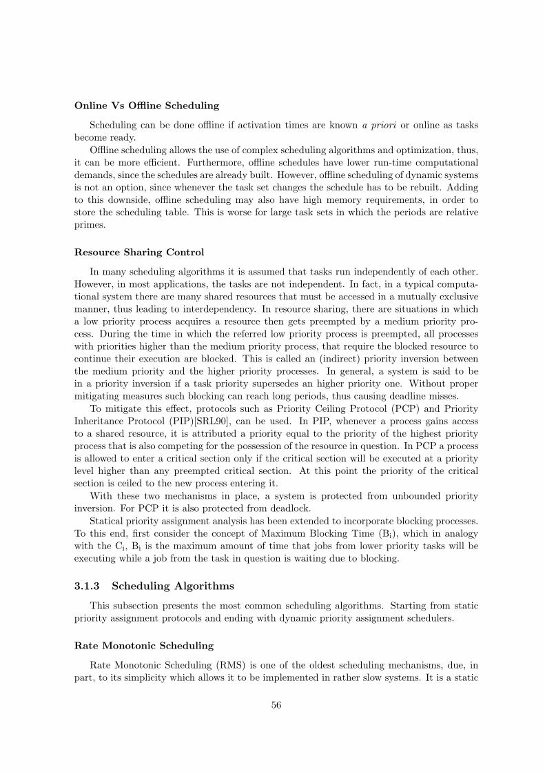
Online Vs Offline Scheduling

Scheduling can be done offline if activation times are known a priori or online as tasksbecome ready.

Offline scheduling allows the use of complex scheduling algorithms and optimization, thus,it can be more efficient. Furthermore, offline schedules have lower run-time computationaldemands, since the schedules are already built. However, offline scheduling of dynamic systemsis not an option, since whenever the task set changes the schedule has to be rebuilt. Addingto this downside, offline scheduling may also have high memory requirements, in order tostore the scheduling table. This is worse for large task sets in which the periods are relativeprimes.

Resource Sharing Control

In many scheduling algorithms it is assumed that tasks run independently of each other.However, in most applications, the tasks are not independent. In fact, in a typical computa-tional system there are many shared resources that must be accessed in a mutually exclusivemanner, thus leading to interdependency. In resource sharing, there are situations in whicha low priority process acquires a resource then gets preempted by a medium priority pro-cess. During the time in which the referred low priority process is preempted, all processeswith priorities higher than the medium priority process, that require the blocked resource tocontinue their execution are blocked. This is called an (indirect) priority inversion betweenthe medium priority and the higher priority processes. In general, a system is said to bein a priority inversion if a task priority supersedes an higher priority one. Without propermitigating measures such blocking can reach long periods, thus causing deadline misses.

To mitigate this effect, protocols such as Priority Ceiling Protocol (PCP) and PriorityInheritance Protocol (PIP)[SRL90], can be used. In PIP, whenever a process gains accessto a shared resource, it is attributed a priority equal to the priority of the highest priorityprocess that is also competing for the possession of the resource in question. In PCP a processis allowed to enter a critical section only if the critical section will be executed at a prioritylevel higher than any preempted critical section. At this point the priority of the criticalsection is ceiled to the new process entering it.

With these two mechanisms in place, a system is protected from unbounded priorityinversion. For PCP it is also protected from deadlock.

Statical priority assignment analysis has been extended to incorporate blocking processes.To this end, first consider the concept of Maximum Blocking Time (Bi), which in analogywith the Ci, Bi is the maximum amount of time that jobs from lower priority tasks will beexecuting while a job from the task in question is waiting due to blocking.

3.1.3 Scheduling Algorithms

This subsection presents the most common scheduling algorithms. Starting from staticpriority assignment protocols and ending with dynamic priority assignment schedulers.

Rate Monotonic Scheduling

Rate Monotonic Scheduling (RMS) is one of the oldest scheduling mechanisms, due, inpart, to its simplicity which allows it to be implemented in rather slow systems. It is a static

56

priority scheduling algorithm.

In RMS, processes are assigned priorities as a monotonic increasing function of their rates,i.e., ∀τi, τj ∈ τ, Ti < Tj ⇒ Pi > Pj .

Classical RMS analysis has a series of assumption, introduced in [LL73] and further dis-cussed in [SKG91]:

• Instantaneous switching between tasks;

• All execution time is dedicated to tasks;

• Tasks do not interact with each other;

• Tasks become ready to execute precisely at the beginning of their periods and relinquishthe CPU only when execution is completed;

• Tasks deadlines are always in the start of the next period (deadlines are equal to peri-ods);

• Tasks with shorter periods are assigned higher priorities, regardless of task criticality;

• A lower priority task is never executed when a higher priority task is ready.

The essentials of RMS analysis were developed in 1973 by Liu and Layland [LL73] where theyshowed that a set of processes is guaranteed to be schedulable if:

U(N) =∑τi∈τ

Ci

Ti≤ N(21/N − 1) (3.2)

where U is the CPU utilization factor, i.e., the fraction of time that the CPU is being used,andN is the number of tasks. The utilization factor converges to ln(2) (≈ 69.31%) asN →∞.

Another schedulability test was presented in [BBB03] and is called the hyperbolic boundtest: ∏

i

(1 +

Ci

Ti

)≤ 2 (3.3)

Both of these are sufficient tests, i.e., U being lower than the test bound is a sufficientcondition for the system to be schedulable. However, they are not necessary conditions, i.e.,if U is higher than the test bound, but with U ≤ 1, then the test is inconclusive. It wasshown in [BBB03] that the hyperbolic bound is tighter than the Liu and Layland bound inthe sense that for every task set that the Liu and Layland bound is verified the hyperbolictest is also verified, however, there are cases in which the Liu and Layland is inconclusive butthe hyperbolic test is conclusive.

RMS is an optimal scheduling mechanism within its assumption set, in the sense that ifexists a scheduler that satisfies RMS assumptions and is capable of schedule a given system,then RMS is also capable of scheduling the system in question.

The fact that U only provides a sufficient condition, prompted the appearance of lessconservative tests, such as the response time test, first introduced in [ABRW91] for theDeadline Monotonic Scheduling, and simplified to the RMS case in [Obe94], and is based onthe fact that was proven in the paper in question: “For a set of independent, periodic tasks,if each task meets its first deadline, with worst-case task phasing, the deadline will always be

57

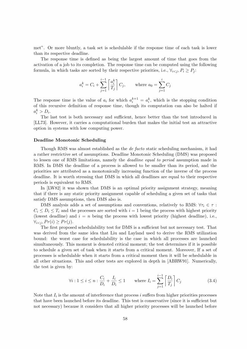
met”. Or more bluntly, a task set is schedulable if the response time of each task is lowerthan its respective deadline.

The response time is defined as being the largest amount of time that goes from theactivation of a job to its completion. The response time can be computed using the followingformula, in which tasks are sorted by their respective priorities, i.e., ∀i<j , Pi ≥ Pj :

aki = Ci +

i−1∑j=1

⌈akiTj

⌉Cj , where a0 =

i∑j=1

Cj

The response time is the value of ai for which ak+1i = aki , which is the stopping condition

of this recursive definition of response time, though its computation can also be halted ifaki > Di.

The last test is both necessary and sufficient, hence better than the test introduced in[LL73]. However, it carries a computational burden that makes the initial test an attractiveoption in systems with low computing power.

Deadline Monotonic Scheduling

Though RMS was almost established as the de facto static scheduling mechanism, it hada rather restrictive set of assumptions. Deadline Monotonic Scheduling (DMS) was proposedto lessen one of RMS limitations, namely the deadline equal to period assumption made inRMS. In DMS the deadline of a process is allowed to be smaller than its period, and thepriorities are attributed as a monotonically increasing function of the inverse of the processdeadline. It is worth stressing that DMS in which all deadlines are equal to their respectiveperiods is equivalent to RMS.

In [LW82] it was shown that DMS is an optimal priority assignment strategy, meaningthat if there is any static priority assignment capable of scheduling a given set of tasks thatsatisfy DMS assumptions, then DMS also is.

DMS analysis adds a set of assumptions and conventions, relatively to RMS: ∀τi ∈ τ :Ci ≤ Di ≤ Ti and the processes are sorted with i = 1 being the process with highest priority(lowest deadline) and i = n being the process with lowest priority (highest deadline), i.e.,∀i<j , P r(i) ≥ Pr(j).

The first proposed schedulability test for DMS is a sufficient but not necessary test. Thatwas derived from the same idea that Liu and Layland used to derive the RMS utilizationbound: the worst case for schedulability is the case in which all processes are launchedsimultaneously. This moment is denoted critical moment; the test determines if it is possibleto schedule a given set of task when it starts from a critical moment. Moreover, If a set ofprocesses is schedulable when it starts from a critical moment then it will be schedulable inall other situations. This and other tests are explored in depth in [ABRW91]. Numerically,the test is given by:

∀i : 1 ≤ i ≤ n :Ci

Di+

IiDi≤ 1 where Ii =

i−1∑j=1

⌈Di

Tj

⌉Cj (3.4)

Note that Ii is the amount of interference that process i suffers from higher priorities processesthat have been launched before its deadline. This test is conservative (since it is sufficient butnot necessary) because it considers that all higher priority processes will be launched before

58

the lower priority ones, and more importantly will terminate before the low priority ones havestarted, which may not always be the case. [ABRW91] presented a, more complex, necessaryand sufficient test based on this observations.

Scheduling Tasks With Arbitrary Deadlines

In Subsection 3.1.3, the principles of schedulability analysis of task sets scheduled underDMS was presented. However, in many real-world applications deadlines are not restrictedto cases in which all of them are not greater than their respective periods.

The DMS schedulability test can be summarized into:

ak+1i = Ci +

∑∀j ∈ hp(i)

⌈akiTj

⌉Cj with a0i = Ci (3.5)

where hp(i) is the set of all tasks that have a priority higher than the priority of task i, ai isthe response time of process i, and aki is the kth iteration of its computation. The test stopseither if aki = ak+1

i or if aki > Di, and the system is schedulable ⇐⇒ ai ≤ Di.

This test is not valid for the case in which exists at least one task with a deadline greaterthan its period, essentially because the computing time of preceding jobs of task i are notaccounted for. To introduce the previous effect, [Leh90] introduced a new concept: busy period- a busy period level i is the maximum amount of time in which jobs of tasks of processeswith priority equal to or greater than the priority of task i may be executed.

Making considerations similar to those made in section 3.1.3, or those that where arguedfor in [Leh90], and later formally shown in [JP86] and [TBW94] it was shown that:

wk+1i (q) = (q + 1)Ci +

∑∀j∈hp(i)

⌈wki (q)

Tj

⌉Cj . (3.6)

In this equation wi(q) is the busy period level i relative to the time interval [t0, t0 + qTi], andwki (q) is the kth iteration of its computation. The computation ends when it converges. The

maximum release time of process i is given by:

ri = maxq ∈ N

(wi(q)− qTi) (3.7)

and the process i is schedulable ⇐⇒ ri ≤ Di.

Since wi(q) is never lower than Ci it is usual to initialize w01(q) = Ci. Similarly, since

wi(q + 1) ≥ wi(q) then w0i (q + 1) = wi(q) is a good initialization value.

This analysis can be easily extended to include the effects of jitter and to the burstybehavior of some processes as it was done in [TBW94].

First Come First Served

In the First Come First Served (FCFS) policy, whenever a process is activated it is at-tributed the smallest priority. As time passes, the process ages, and its priority increases.The highest priority process is scheduled next.

FCFS is one of the simplest possible dynamic priority assignment algorithm, hence it hasfound applicability among systems with low computational capabilities.

59

A task set is FCFS schedulable if, even if, all tasks arrive simultaneously in the queue,without considering re-arrivals, it is still schedulable; i.e.

∀i:τi∈τ∑

j:τj∈τCj ≤ Di (3.8)

Earliest Deadline First

Earliest Deadline First (EDF) is a dynamic scheduling priority assignment algorithm.In EDF the next job to be scheduled is the job with earliest (nearest) deadline. It has autilization bound of one, assuming that all deadlines are equal to their respective periods,i.e.,

U =∑i:τi∈τ

Ci

Ti≤ 1. (3.9)

In so being, EDF is an optimal scheduling policy, among dynamic priority assignment policiesin which all processes deadlines are equal to their respective periods, since no scheduling policycan achieve utilizations higher than one.

A priority assignment algorithm is said to be predictable under overload if whenever sometask set is not schedulable, then it is known a priori which subset of the task set will not bescheduled. This is the case of RMS and DMS, but is not the case in EDF.

EDF has two main disadvantages: it introduces a considerable overhead during its dynamicpriority assignment and it is not predictable under overload. These two factors have delayedEDF industrial deployments despite its wide acceptance in the research community.

EDF is optimal even when deadlines are smaller than their respective periods, and in thatsituation the following is a sufficient but not necessary test:

U ′ =∑i:τi∈τ

Ci

Di≤ 1 (3.10)

The last test is equivalent to increase the utilization, since U < U′, and due to its sufficiency,when it holds then the task set is schedulable. However, if it does not hold then more complextests are required.

A formal analysis of EDF with deadlines not greater than their respective periods wasmade in [Spu96] and [LG96]. Here some results are presented. To perform a sufficient andnecessary test it is necessary to introduce a new concept, namely the Demand Function.

The demand function of a process is defined as the amount of computation necessary tobe done between instants t1 and t2 so that the process is schedulable. Or putting it moreformally:

dfi(t1, t2) =∑ai≥t1di≤t2

Ci (3.11)

where ai is the moment at which process i was activated, di is the deadline of process i, andCi is the amount of computation performed by process i. So in a sense the demand functionof process in an interval [t1, t2] is the worst case amount of computation that process i has toperform in that period.

60

The demand function of a set of processes on a given interval is defined as the sum of thedemand functions of each of its processes:

df(t1, t2) =∑i:τi∈τ

dfi. (3.12)

The definition of demand function implies that “A task is (EDF) schedulable if ∀t1, t2 :t2 > t1 df(t1, t2) ≤ t2 − t1”. For example, computing in 5 seconds what the hardware canonly compute in 6 seconds is impossible. This remark provides a necessary and sufficientschedulability test for EDF. However, it would be necessary to test an infinity number ofintervals in order to decide about the task set schedulability. To overcome this hurdle, thenotion of critical moment introduced earlier in this section must be incorporated. So consideronly the situation in which at the instant t = 0 all processes are activated. So, the testbecomes:

∀t df(0, t) ≤ t (3.13)

The last observation induces the definition of a new measure, namely the Demand BoundFunction:

dbf(L) = maxt

(df(t, t+ L)) = df(0, L). (3.14)

Equation (3.14) defines a unidimensional function, which can be used is a unidimensionaltest, as opposed to a bi-dimensional test in t1 and t2), but it still necessary to test an infinitynumber time instants. If all processes of the set are periodic then it is possible to reduce itto a finite number of test based, for example, up to the least common multiple of all periods.The resulting test range is denoted L∗. Note that this test does not need to test all the instantof the interval in question, it suffices to test the instants in which the dbf changes.

Least Slack First

The Slack of a process is defined as the maximum amount of time that its execution canbe delayed while still meeting its deadline.

Least Slack First (LSF) or Least Laxity First (LLF) is a scheduling algorithm that wasproposed to deal with a deficiency of EDF: in EDF the next process to be executed is alwaysthe one with the closest deadline, even if there is another process that will meet its deadlineonly if scheduled next, due to its high execution time.

LLF tries to improve EDF by executing the process with the lowest slack. Therefore,situations as those described above do not result in a failure to meet the deadline.

However, LLF has a high temporal locality LLF is local in the sense that the slack usingin the scheduling is computed in a given time instant and will not be equal in the followinginstants. LLF’s high temporal locality causes two problems, one of them being thrashing thatoccur whenever two or more jobs have the minimum slack of the system. Whenever one ofthem is scheduled, after running for a unit of time, the other becomes the job with the leastlaxity.

[HGT99] proposed a solution for the thrashing problem: whenever two or more processeshave the same slack the one with lowest deadline is executed and the others are excluded.These processes continue excluded until the execution of the current process is halted oris preempted by another process. A process may preempt an excluding process if it is notexcluded and its laxity is the lowest in the system.

61

Another solution to the thrashing problem is given in [WD07]. This solution builds uponthe previous one and is based on fuzzy rules (thresholds). [WD07] presents many solutionsto the thrashing problem that are between the two presented in this section.

Servers

Aperiodic servers emerged to fill the necessity to include aperiodic tasks in the model set.Servers allow to schedule together periodic and aperiodic tasks, while guaranteeing that thelater have a desired priority level and a bounded interference on the former.

Aperiodic servers are defined by their replenishment period and an execution budget. Anaperiodic server is a logical task created to handle randomly arriving requests, with a priority,replenishment periods and execution budget attributed based on some scheduling policy. Theexecution budget of a server is diminished each time that it handles a request. The serveritself acts as a periodic process to which resources are attributed, moreover, it is defined asany regular process τi.

The simplest aperiodic server is the background server. Basically, whenever there are noready periodic tasks, the background server attributes the execution to the highest priorityaperiodic task, if any. Under this server the aperiodic tasks have no influence over theschedulability of periodic tasks. Furthermore the aperiodic ones have the lowest priority ofall. This raises serious constrains since the periodic tasks may never be all in simultaneousidleness, causing the aperiodic tasks to never be executed.

To solve this problem, the polling server was introduced. The polling server has a givenperiod, priority and execution time, like any other periodic tasks. When it is scheduled, itpolls the aperiodic tasks associated with itself, and if the ready queue of aperiodic tasks isnot empty it executes the higher priority one. The complexity of this server is comparableto the complexity of the background server. Under this, server aperiodic tasks interfere withperiodic ones in a controlled and bounded way and their priority is not necessarily the smallest.However, aperiodic tasks have a poor reactivity, since if they are activated immediately afterthe pooling server, they must wait a full period, even if the server has not executed, asillustrated in Figure 3.1.

0 5 10 15

t1

ts

t3

2

Task ID T C1 3 1

s 4 1

3 6 1

Asynchronous request of x time units

x

Figure 3.1: Example of an Aperiodic Server — Polling Server, aperiodic jobs were releasedsooner, but were executed only at the polling instants

To solve this issue it was introduced the deferrable server. The deferrable server differs

62

from the polling server because if the deferrable server becomes the highest priority task, itonly executes if there is an aperiodic task associated to it waiting for execution, furthermore,in these instants its capacity is not spent. Otherwise, it defers its execution until such instant.In the deferrable server, provided that there is capacity available to do so, aperiodic taskscan be served at any time during the server period. This solves the main issues of the pollingserver. Nevertheless, it introduces another one, namely this server interferes with periodicprocesses in a way that is not equivalent to a periodic task, thus reducing the schedulabilitybound of the system and increasing the response time of periodic processes. For instance, onesuch interference is under RMS, in which the assumption that active tasks execute wheneverthey become the highest priority tasks.

One of the servers introduced to solve the problems in the deferrable server is the sporadicserver. In the sporadic server the execution budget is not replenished in the beginning of eachperiod. While in the polling Server and the deferrable server, the budget is replenished peri-odically, in the sporadic server the replenishment is normally scheduled whenever the servercapacity starts to be consumed. The sporadic server is more complex than the backgroundserver.

There are also servers for dynamic priority systems, such as the Total Bandwidth Server(TBS) [SB94] and Constant Bandwidth Server (CBS) [AB98].

3.2 Real-Time Communication Networks

The last decades were marked by a steady development of real-time communication net-works, fueled by the steady development of automation that took place in the industry.Informally, a Real-time communication network is a set of communication links placed toprovide connectivity between field devices, e.g. sensors, actuators, controllers.

Real-time communication architecture differ from general purpose communication sys-tems mainly because Real-time communication network have to meet specific real-time re-quirements, namely: efficient short messages handling, support periodic and aperiodic traffic,bounded response time, redundancy, low implementation and maintenance costs.

In the remainder of this section an overview of some basic Real-time communicationconcepts will be presented as well as an overview of some of the most relevant Real-timenetwork protocols.

3.2.1 Real-Time Communication Architecture

Real-time communications are usually implemented based on some kind of layered mul-tiple access networks communication architecture [MZ95]. Each layer has a set of protocolsresponsible for carrying out specific operations that are made available to higher layers. Fig-ure 3.2 shows the architecture of the International Standard Organization (ISO) ReferenceModel for Open Systems Interconnection (OSI) [Con10]. However, real-time communicationnetworks frequently employ a collapsed OSI-based architecture, in which the upper 5 layersare merged into a single application layer, as shown in Figure 3.2.

Following this philosophy the following layers are not usually implemented in real-timecommunication stacks: application interface, providing common services required to the par-ticular applications; presentation layer, to provide a vendor independent data access, in orderto allow for interoperability; session layer, to allow opening and closing dialogs betweensenders and receivers; a transport layer, to handle end-to-end communications; a network

63

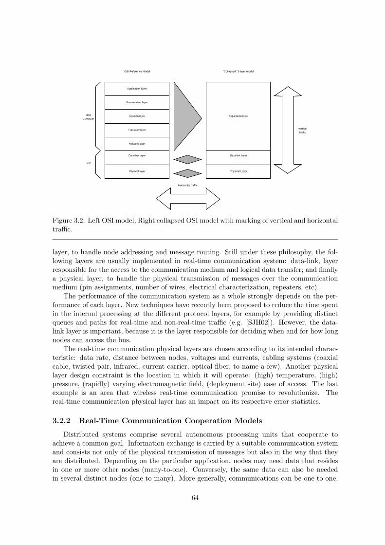
Application layer

Presentation layer

Session layer

Transport layer

Network layer

Data-link layer

Physical layer

HostComputer

NIC

Application layer

Data-link layer

Physical Layer

OSI Reference Model "Collapsed" 3-layer model

vertical traffic

Horizontal traffic

Figure 3.2: Left OSI model, Right collapsed OSI model with marking of vertical and horizontaltraffic.

layer, to handle node addressing and message routing. Still under these philosophy, the fol-lowing layers are usually implemented in real-time communication system: data-link, layerresponsible for the access to the communication medium and logical data transfer; and finallya physical layer, to handle the physical transmission of messages over the communicationmedium (pin assignments, number of wires, electrical characterization, repeaters, etc).

The performance of the communication system as a whole strongly depends on the per-formance of each layer. New techniques have recently been proposed to reduce the time spentin the internal processing at the different protocol layers, for example by providing distinctqueues and paths for real-time and non-real-time traffic (e.g. [SJH02]). However, the data-link layer is important, because it is the layer responsible for deciding when and for how longnodes can access the bus.

The real-time communication physical layers are chosen according to its intended charac-teristic: data rate, distance between nodes, voltages and currents, cabling systems (coaxialcable, twisted pair, infrared, current carrier, optical fiber, to name a few). Another physicallayer design constraint is the location in which it will operate: (high) temperature, (high)pressure, (rapidly) varying electromagnetic field, (deployment site) ease of access. The lastexample is an area that wireless real-time communication promise to revolutionize. Thereal-time communication physical layer has an impact on its respective error statistics.

3.2.2 Real-Time Communication Cooperation Models

Distributed systems comprise several autonomous processing units that cooperate toachieve a common goal. Information exchange is carried by a suitable communication systemand consists not only of the physical transmission of messages but also in the way that theyare distributed. Depending on the particular application, nodes may need data that residesin one or more other nodes (many-to-one). Conversely, the same data can also be neededin several distinct nodes (one-to-many). More generally, communications can be one-to-one,

64

one-to-many, many-to-one and many-to-many.

Figure 3.2, beside presenting the aforementioned OSI and collapsed-OSI reference models,also presents the concept of vertical traffic and horizontal traffic among two nodes. Horizontaltraffic is depicted by the horizontal line as spanning both nodes, and vertical traffic as spanningthe several layers of each node’s protocol stack.

The client-server is a data exchange model, in which nodes that are sources of some databehave as servers. Nodes that need the data (clients) issue requests to the respective server,which in turn replies with the data in question. This communication model is inherently one-to-one, and can lead to both spatial and temporal data inconsistency problems when usedto support one-to-many or many-to-one communications. For instance, if the same data isrequired in several nodes, different nodes issue the respective requests to the server. If thedata value changes during this period, the successive replies of the server will carry differentvalues of the same entity, resulting in spatial inconsistency. On the other hand, when a nodeneeds data from different servers, it must issue the requests sequentially, one after the other,which can result in temporal inconsistency. Another problem posed by this model is relatedwith the internal servers scheduling and processing of requests.

Data exchanges can also be defined in terms of producer-consumer, as opposed to client-server. In the producer-consumer framework, as introduced in [TN89], a given physical vari-able, e.g. temperature, is associated to a system variable. Entities that generate or convertthe physical value into the respective system value are called producers (of the referred vari-able). The producer-consumer model associates unique logical handles to each message type.Messages are generated and received based only on these logical handles, without any explicitreference to the message’s source or destination nodes.

Due to its broadcast nature, the producer-consumer model inherently supports one-to-oneand one-to-many communication, without causing spatial data consistency problems. How-ever, this property may be lost if the underlying network does not support atomic broadcasts.

This model, however, does not solve the problem of temporal consistency, that can beintroduced, for instance, by the contention resulting from a multiplicity of producers on thenetwork. This problem has been solved by the producer-distributor-consumer (PDC) model[TN89], which adds coordination to the producer-consumer model. In the PDC model theproducers behave as slaves with respect to an arbitrator node. Such node is fed with themessage properties and temporal requirements of the messages that are exchanged in the busand builds a suitable schedule, which, is then used to grant to a single producer at a time theright to transmit.

Real-time communication systems are comprised of two types of traffic [FV92]: 1) Verticaltraffic which is comprised mainly of requests from upper-level entities to lower level entities,and subsequent confirmations (acknowledgments) from lower level entities to higher ones; thistype of traffic follows a client-server philosophy. 2) Horizontal traffic which is comprised ofdata exchange between entities of the same layer, e.g. between the physical layer of a sensorand a controller, or between the application layer of two controllers. Note that in the lattercase, for the correct exchange of horizontal information, vertical exchanges would also benecessary.

Traffic Model

Real-time communication systems normally include time specifications. These specifica-tions are used to verify if a set of messages can be delivered in a manner that guarantees

65

the coherence of actions and/or data. The most used time specifications are: periodicity,jitter, application process response time, and some possible relations between the timingspecifications of two different messages.

The periodicity, in this context, refers to the (minimum) amount of time between twotransfers. The jitter is a measure of time variation in relation to a pre-specified time set.As examples of possible real-time communication jitters include, the transmission instant,the reception instant, transmission duration, etc. For instance, [But97] defines two typesof jitter, relative jitter, which is the maximum deviation of the start time of two con-secutive instances RRJi = maxk (si,k − ri,k)− (si,k−1 − ri,k−1), where si,k is the startingtime of the kth instance of ith task and ri,k is the respective release time; and [But97]also define absolute jitter as the maximum deviation of the start time among all instances:ARJi = maxk (si,k − ri,k)−mink (si,k − ri,k). High (relative) values of jitter degrade the qualityof the real-time communication.

The response time is the (maximum) delay between a request and a confirmation, orbetween a demand and a response, or any other two similar events. Response time can bemeasured either locally, for example, time from the moment that the request was sent to whenthe response was received or between distributed occurrences. For more in time constrains ofreal-time communication systems, refer to [Des85].

Real-time communication are used to transmit data between distributed control elements.Most of this traffic is periodic in nature, with a periodicity that is defined by the controlalgorithm. Thus, this type of traffic is time-triggered (or at least time-driven), in the sensethat it occurs when a given instant is reached. Another type of traffic is called event-triggeredand it occurs when a given event takes place. Event-triggered transfers are particularly usefulfor variables that do not change their values regularly. A deeper analysis of periodic andaperiodic (time/event-triggered) traffic (or messaging) is performed in [Kop91].

3.2.3 Real-time Communication Medium Access Control

Real-time communication systems Medium Access Control (MAC) protocols can be di-vided into two main classes: controlled and uncontrolled. A MAC is controlled if there is asignal (explicit or not) that informs the nodes about who is next to transmit, hence preventingthe occurrence of collisions. In uncontrolled MACs there is no (global) arbitration scheme,therefore collisions may happen. Usually, in such cases, measures are taken to prevent and/ordetect the occurrence of such collisions.

A controlled MAC is said to be centralized if there is a (central) node that handles themessaging schedule, otherwise it is said to be distributed. In distributed unontrolled MACs,all nodes willing to transmit in a given time slot/frame are involved in the arbitration. Thesenotions and other related with fieldbuses are discussed in detail in [Tho98].

Controlled MACs provide real-time guarantees, are predictable, thus are appropriated tocontrol application; however, most controlled MACs are inflexible. Uncontrolled MACs areflexible but tend to not provide real-time guarantees.

The controlled MACs presented so far are (mostly) static, always behaving in the sameway. For introducing some dynamic behavior, thus allowing the MAC to be more adjustableto the situation in hand, [Foh93] proposes a mechanism that allows the MAC to have differentoperating modes. In many protocols that implement CSMA-CA there is already a dynamicbehavior, in which the protocol suggests different values for transmission and pre-transmission(waiting to confirm that the medium is free) windows, for depending in the medium usage:

66

idle vs congestion.

Examples of uncontrolled MAC protocols include: all protocols based in Carrier SenseMultiple Access (CSMA) as BATIBUS (French Standard NFC 46620), EIBUS (EuropeanInstallation Bus), EHS, LON, CAN [Rob91], Ethernet [Soc08]. The first four use a simpleversion of CSMA, CAN uses CSMA Non-destructive Bitwise Arbitration (CSMA-NBA), Eth-ernet uses CSMA-CD where CD stands for Collision Detection, which allows nodes to sensea collision and stop transmitting. Other versions of CSMA include CSMA-CA (CollisionAvoidance), though this version is primarily used in wireless systems. Wireless fieldbuses arenow starting to enter in the control arena, as in the case of wirelessHART [wa].

Examples of centralized controlled MAC protocols include: some tokens passing protocols,and master polling. The representatives are: Profibus-PA, WorldFIP [AC98], P-Net, Interbus-S [Int87], ASI. Possible TTP [KG94] and [KAGS05] are the most widely deployed decentralizedcontrolled MAC.

3.2.4 Effects of Available Real-Time Communication Networks on Net-worked Control

As mentioned on Section 2.1, control networks require a physical implementation, thatnowadays, due to the development of certain key technologies, is accomplished by the use ofreal-time communication networks.

The real-time communication networks have an enormous effect on the quality of controlof the systems that operate under it. Due to the inherent characteristics, such as latency, bitrate, message jitter and associated synchronization metrics, minimum and maximum messagesize and packet drop rate and the presence/lack of of an associated packet acknowledgement.

Regarding the latency (and the sampling to actuation delay, which are normally lumpedinto the average dead-time of the system), it is low varying by nature, since the fast varyingcomponent is accounted for in the jitter. For this reason, it is possible to compensate for itat the control level. As for the bit rate, higher bit rates, can in principle, allow for controlusing smaller sampling times. Nonetheless, will be discussed in this Thesis a mechanism thatdecouples the fieldbus sampling rate from the control sampling rate that is effective if thesystem dynamics is well known.

The jitter can have a nefarious effect on the quality of control and it is relatively difficult tocompensate for at the control level. For this reason, some real-time communication networkshave an isochronous mode, i.e., low jitter, as will be presented in this section. Nevertheless, itis possible to ease the effects of jitter by trading latency for jitter, i.e., use a synchronizationpoint at which it is guaranteed, with a given probability, that the message will have beenreceived.

Current real-time communication networks, i.e., the Ethernet based ones, have minimummessage sizes that are larger than the size of an average control message. The extra spacecan be used to send data that normally would not be sent.

The packet drop rate and the message reception acknowledgement are two fundamentalaspects of lossy networks that, as will be discussed in Thesis, can be essential to optimallycontrol this type of networks.

67

3.2.5 Available Real-Time Communication Networks

In this subsection, a summary description of some available fieldbuses is made. Amongthe many types of fieldbuses that exist, were chosen those that either are representative oftheir class of fieldbuses, thus are a landmark in understanding fieldbuses, or have gained asignificant acceptance among the industrial networking community. Given these criteria thereare presented at Appendix A the following protocols: CAN, TT-CAN, FTT-CAN, CANopen,TT-Ethernet, Ethercat, TTP, Ethernet POWERLINK, FlexRay, Profinet and WorldFip.

Table 3.1 summarizes the most relevant features of such fieldbuses.

3.3 (m,k)-firm Systems

Nowadays, the use of electronic devices is widespread into virtually all sectors of modernlife. Moreover, virtually all such electronic devices can have more than one task, renderingthe scheduler a paramount piece of the software puzzle.

Most such devices model their tasks in a restrictive manner, allowing only for the existenceof the two types of task, i.e., hard and soft. However, as will be seen in Section 3.3.1, thereare situations in which there is a need for tasks that are neither hard nor soft, but can toleratethe miss of a number job executions.

Remembering that a scheduler is said to be optimal, within a given class, if for every taskset that can be scheduled by an algorithm that belongs to this class, can also be scheduledby the scheduler in question. In particular, an (m, k)–firm scheduler is said to be optimal ifit can schedule all feasible (m, k)–firm systems. However, in (m, k)–firm systems there is alsoa drive to maximize the utilization of the system, either on a fairly manner or not. This factintroduces a new optimality constraint, namely that the optimal scheduler must also achievethe highest possible utilization.

The classification of (m, k)–firm schedulers that is employed in this Thesis was introducedin [JYQ06] and the prime reason for choosing this classification is its relevance for the correctunderstanding of the interplay between (m, k)–firm and control systems. The classification inquestion is done according to the system determinism and they are classified into determin-istic or classical — which are explored in this Thesis — and probabilistic, which are moreconcerned with probabilistic guarantees. In deterministic (m, k)–firm systems, in every group

Protocol Bitrate Jitter Latency Cycle Topologies Real–Time

Philosophy

CAN – – – – – – No Basic Yes Peer–to–PeerTTCAN – – ± – – Yes Basic Yes Master–SlaveFTTCAN – – ± – – Sync/Async Basic Yes Master–Slave

CANopen – – – – – No Basic Yes Exported Functionalitiesover Peer–to–Peer

WorldFIP ± – – Yes Complex YesProducer/distributer/consumer

FlexRay + ± ± No Complex Yes Segmented Peer–to–PeerTTP + + + Yes Basic Yes Master–SlaveTTE ++ + + Yes Basic Yes Master–Slave

EtherCAT ++ – ± No Complex YesMaster–Slave w\packet concatenation

EthernetPowerlink

++ ++ ++ 3 part cycle Basic Yes Master–Slave

PROFINET ++ ++ ++ 3 part cycleExtra layerof supervision

Yes SupervisedMaster-slave

Table 3.1: Most prominent Fieldbuses and their most relevant characteristics.

68

of k consecutive periodic activations of an (m, k)–firm task there are at least m executions,which is in contrast with probabilistic (m, k)–firm systems, where the ratio between activatedand executed jobs, for a large number of activations, must be no smaller than m/k.

A task is said to be in a dynamic failure if on the last set of k periodic job activations,there were less than m job executions. Evidently, under deterministic (m, k)–firm scheduling,tasks are supposed to never be in a dynamic failure.

In the strict sense, static schedulers cannot execute the jobs that they mark as optional,since the execution of these jobs may either jeopardise the completion of mandatory jobs,hence, causing the system to enter a dynamic failure or imply some form of policing toguarantee the timely completion of the mandatory jobs, thereby rendering the overall systema dynamic scheduler. Furthermore, if a given static job that belongs to a repeating cycle isguaranteed to complete without causing any mandatory job to fail, then it is worthwhile toset it as mandatory as well.

3.3.1 Related Work

In [Ram99] it was put forth an implementation which managed to gather a significativemomentum in the community. It was first proposed that the scheduler should divide itstask’s jobs into mandatory and optional ones. Each group of k consecutive jobs should havem mandatory jobs. This was in total contrast with the then established use of distance tofailure. Jobs are set as mandatory/optional based on an upper mechanical word, defined as

a =

⌊⌈ami

ki

⌉kimi

⌋. (3.15)

in which a is the number of the job instance, i.e., τi is activated at instant aTi, a = 0, 1, 2, . . ..Whenever the previous condition is verified the job is set as mandatory, otherwise it is set asoptional. For example, for an (3, 7)–firm task, the first seven executions, of the right-side ofEquation (3.15), in which the first one has a = 0, would be equal to [0 2 2 4 4 7 7], hencegenerating the (3, 7)–firm frame [1 0 1 0 1 0 0]. The frames generated by the rule definedin Equation (3.15) are called upper mechanical words and it generates an evenly distributedmandatory activation pattern. In [BC01] this model was expanded by first considering normal(optional) and panic (mandatory) jobs (thus a bimodal scheduler), and then trying to providea schedule of panic jobs that guarantees that they will always meet their deadlines. However,there approach was not based in upper mechanical words or other mathematical extensions,but rather on the authors intuition of what the repeating frame should be. A contributionfor this approach is given in [LC06], in which it is proposed that the mandatory jobs shouldbe assigned in a manner that minimizes a certain metric, dubbed Granularity of Quality ofService-Reward (-reward).

In [QH00] it was discussed the fact that the scheduler presented in [Ram99] introducesa periodic critical instant, of which, one of the instances is at t = 0. Thus, the even distri-bution of mandatory jobs is not necessarily the best one. This led the authors to proposethree different algorithms for finding a suitable schedule for the mandatory tasks. Thesealgorithms differ primarily in their computational efficiency. The first resembles a test ofall possible schedules, the second is a genetic algorithm that at each round tests the taskset for schedulability, the third one introduces a metric that drives the search parameters ofthe genetic algorithm. Notwithstanding the exhaustive nature of the proposed algorithm, ingeneral, it fails to reach the optimal schedule because, as will be shown in this Thesis, the

69

search space of the algorithm is smaller than the solution space. Furthermore, the solutionsthat the paper proposes are still haunted by the problem that it intended to solve, namely,in many situations, the proposed scheduler introduces the same type of critical instants thatwere introduced by the upper mechanical words of [Ram99], though it introduces them indifferent instants.

A different type of static pattern was presented in [KS95], the so called Deeply Red (orR-) pattern and is defined by setting all jobs that verify

ji mod ki < mi (3.16)

as mandatory and setting the remaining ones as optional, where ji is a non-negative integerthat is incremented by one whenever a job from the task in question is released. Note that ifji = 0 at the release of the first job of the task, then the generated static sequence will consistof mi mandatory jobs in the beginning of the cycle, obviously, followed by ki −mi optionaljobs. For example, for a (3, 7)–firm task that is initialized with j = 0, then the sequencewould be [1 1 1 0 0 0 0]. If ji = 0 at the release of the first job of the task, then there willbe a phase, equal to ji on the previously defined sequence. Thus, for a certain extent, theparameter j can be used to introduce a relation of phases between tasks, but it is absolutelyimpossible to escape from a critical instant if there is no special relation among the task’speriods.

It was proved in [NQ06] that if a given (m, k)–firm task set is schedulable using a DeeplyRed pattern then it is schedulable using any other static k jobs sequence with m job activa-tions, which also follows from the above discussion regarding critical instants. However, thisis not the same as optimality which implies that if there exists a scheduler that can schedulea given system, then the proposed scheduler can also schedule the system in question. In fact,the proof presented in [NQ06] proves that there is no scheduler, in the set of schedulers thatuse a static frame with the respective (m, k)–firm properties, that performs worse than theDeeply Red pattern.

In [JYQ06] it is noted this limitation regarding the provisioning of deterministic (m, k)–firmguarantees using static frames of length k with m job activations and it argues that the de-terministic approach “does not contribute to reducing the resource requirements in general”.However, this conclusion is based on 1) static frames introduce critical instants, 2) tasks withimplicit deadlines can be scheduled starting from a critical instant if, and only if, the task setis also EDF-schedulable, therefore, 3) all task sets that provide deterministic guarantees areEDF-schedulable. However, at the core of such line of reasoning is the assumption that theresults of [QH00, Ram99] and other contemporary (m, k)–firm proposals are optimal. But, aswill be shown in this chapter, contemporary schedulers are suboptimal in such a manner thatthey introduce critical instants, that in turn validate the remarks made in [JYQ06]. However,the generalization that is made in the paper in question is not warranted.

Regarding the implementation end of the field, consider what (to the best of the author’sknowledge) was one of the first papers to tackle the problem of (m, k)–firm scheduling and isreported in [HR95], in which it was presented a scheme in which messages were supposed toachieve probabilistic (m, k)–firm guarantees by attributing to each task a distance to failureand attribute higher priorities to tasks with lower distances, i.e., closer, to failure. Thedistance to failure is the number of future consecutive jobs/messages that have to not beexecuted in order to put the task/message in a dynamical failure. In case of a draw, i.e.,several tasks with the same difference to failure, its choice was made based on EDF. This

70

approach was dubbed Distance Based Priority (). DBP had a number of downturns thatstemmed from the fact that the algorithm had no awareness of tasks periods and deadlines,nor the relationships among them. A similar approach was put forth in [Kim10], in which an(m, k)–firm model for wireless networks was presented. The authors introduced some aspectsrelevant to wireless networks such as the distance to the sink (signal strength). However,in general, it inherited all the issues of its predecessor. Furthermore, it only minimizes theprobability of a failure, thereby not providing any guarantee that (m, k)–firm constraints willalways be met, i.e., it is a probabilistic (m, k)–firm scheduler. Such probabilistic approachwas first proposed in [KKH04].

Other variants of DBP include Integrated DBP () [ZWxS04], which used not only thedistance to failure but also the distance to recovery upon failure, that is not very effective atavoiding a system’s entrance into dynamic failure, but significantly reduces the domino effectin which, as in EDF, the failure in one job/task is propagated into other jobs/tasks. Matrix-DBP ( [CSWS04], also uses the distance to failure to schedule message streams, but it differsat a fundamental level from other variants since, by virtue of its intended purpose, it cannotbe preemptive. It employed a rather large set of other variables such as periods, (execution)service time and relationship between streams. An expanded version of the matrix-DBPinto the , which allows for non-periodical messages was presented in [CSWS04]. Also [LY08]improves upon DBP introducing a Total BDP () which introduces a total distance to failurethat include other relevant parameters, such as distance to enter invalidation (dynamic failure)and to exit it, which in much resembles the goals of IDBP [ZWxS04].

In [KC11] it is presented a multiprocessor implementation of a protocol of the DBP family.An analysis of its probability of being in a dynamic failure is also presented. In [LK12]it is proposed a protocol called Local DBP () which has the goal of providing (m, k)–firmguarantees to multimedia streams over wireless sensor networks. It works by augmenting thedistance of DBP with local node information regarding link congestion and failure rates.

In [Eve10] it is discussed the possibility of performing an online schedulability test thatadmits optional jobs if and only if it can be assured that they will not cause a mandatory jobto miss a deadline. This is further enforced by putting the jobs into two different executionqueues, a high priority queue for mandatory jobs and a low priority one for optional jobs, withjobs from the low priority queue executing if and only if the high priority queue is empty. Theproposed schedulability test is not tight, in the sense that it is possible that an optional jobcan execute without causing any deadline miss of a mandatory task but it gets declined by thescheduler. This phenomenon is sometimes called a false negative. The approach presentedin this Thesis also uses an online schedulability test. However, the proposed approach is lessrestrictive, in the sense that optional jobs are allowed to interfere with mandatory ones foras long as they do not cause a deadline miss.

In [CCP10] it is presented the approach that is most similar to the one presented herein.The authors use both the time to failure approach (DBP) and a deadline awareness that mit-igate some of the issues related to the original DBP. Two algorithms are presented, the guar-anteed on-line scheduling algorithm () being the most powerful, the other being a lightweightversion with a lower computational demand. In GDPA it is decided to put a given job in theexecution queue based on a local (temporal) state of the queue. Thus it can put a job thathas a long distance to failure in the queue (as long as there are no jobs of tasks with lowerdistances at the moment) while in the following scheduling instant a job from a task close toa dynamic failure is released, which cannot be executed because the queue is already full. Anexample of this effect is explored in-depth in this Thesis.

71

Applications of (m, k)–firm scheduling in control are presented, for example, in [Ram97] inwhich the fact that many control applications are resilient to a small number of failures is usedto reduce the resource usage. Controller modifications are also discussed. In [LSSL06] thegraceful QoS degradation provided by (m, k)–firm scheduling is explored. More concretely,DBP is analyzed and sufficient, though not tight, conditions for deterministic schedulabilityand their applications for control purposes were proposed. [FNSLY08] tries to devise anoptimal (m, k)–firm frame (repeating pattern) for control purposes. However, the approachpresented therein did not made any consideration regarding the schedulability of the resulting(m, k)–firm sequence, which could potentially invalidate the underlying assumptions. In fact,this is a general issue regarding the utilization of contemporary (m, k)–firm schedulers forcontrol, i.e., they do not guarantee the schedulability of the respective (m, k)–firm tasks,which in turn causes a series of obvious problems. Furthermore, the authors used a rathershort integration time in their ISE computation, thus sequences that had mandatory tasksin the beginning of the meta-frame ended up having lower ISE, even among sequences thatwere rotations of one another.

Moreover, the actuation scheme that was used in the control related contributions share acommon problem, namely, though the schedulers assume that optional jobs may or may not beexecuted, the controllers are designed assuming that optional jobs will never be executed. Themain problem caused by this assumption disparity is that upon the reception of an optionalmessage, the controller will assume the reception of a mandatory message in its respectivetime, thus generating the corresponding control value, which obviously will be erroneous.Additionally, upon the reception of the next mandatory message, the controller will assumethat it is receiving the mandatory message that would follow that one, and so on. To the bestof the author’s knowledge, the only controller that does not have this problem is [CeSP11],which was proposed by the authors of this Thesis and presented in Chapter 4 and Chapter 5,and the main reason why this controller does not have this problem is that it uses sequencenumbers that allow it to find out how many messages/jobs have passed since the last one wasserved.

In [WJ08] it is presented a study of the application of (m, k)–firm schedulers in multimediasettings, with a special focus on the DBP scheduler. Multimedia is one of the areas in which(m, k)–firm scheduling has the potential to provide considerable improvements, as can beattested in [WJ08] and references therein. For example, for the JPEG video case, thereare two types of frames. The most important type (key frames), used to decode the otherless important frames, must always be sent, which conflicts with many dynamic schedulers,because dynamic schedulers do not provide guarantees regarding which job will be executed.For example, DBP only cares about the distance to failure, completely disregarding theimportance of the associated frame.

3.4 Feedback Scheduling

The co-design of real-time systems and networks with their respective applications, whichusually is control, led the various applications that have time varying computational demands.For example, if the controllers are allowed to change their sampling periods, then it would bereasonable that the minimum inter-arrival time of their respective tasks are also allowed tochange. Moreover, there is a need to choose the parameters of such tasks in a manner thatoptimizes, or that at least provides some guarantees, regarding the behavior of the application.

72

This fact stimulated the development of schedulers with the aforementioned characteristicsand they are called feedback schedulers and are roughly defined as any scheduler that considerthe current state of the system on its scheduling decisions.

In [LSST02] it is presented an extensive discussion on the application of control theoreticalapproaches to feedback scheduling. Their approach use the transfer function approach todevise feedback controllers with zero static error, i.e., the actual task utilization is equalto the user specified value, and with some requirements regarding the transitory behaviour.Nevertheless, the approach is applied to only one task at a time, with little regard to the factthat the sum of such utilizations is equal to a constant, i.e., one. This approach is appliedfor the dynamic scheduling of multiprocessor systems in [SCH11]. This framework is also in[YZL+12] for scheduling a systems that change their operating frequency, hence its effectiveutilization, in order to deal with processors’ thermal fluctuations. The framework in questionis used in the scheduling the inner loop, i.e., the actual tasks parameters.

In [APLW02] the authors explored the concept of reservation applied to feedback serverscheduling. In this context, each server would reserve a certain amount of time, i.e., a periodand maximum utilization that it will require on such amount of time. The scheduler uses acontrol theory based approach to schedule the various servers. [Lin07] presents an extensivesurvey of reservation based feedback server scheduling. However, it must also be noticed thatthis has not been an active area of research on the last years.

In [SLB08] it is considered the possibility of dynamically changing requirements, i.e.,period and capacity, of servers of static priority processes in a feedback scheduling scenario.This work, though from the same authors, differs from the past because it allows for onlinescheduling. Requests that reduce the utilization of servers are handled seamlessly. However,requests to increase the requirements are handled by first performing a schedulability test toensure that of the new task. If the new task set is schedulable, then the request is processed,otherwise the server in question is given the highest utilization that is schedulable. The paperproposes five different schedulability test algorithms with different degrees of tightness andcomplexity.

In [BLCA02] it is presented the elastic model, which is also a type of feedback scheduler.The elastic model is based on an analogy between with of strained springs and a series oftask weights. Each task has an individual weight, such weights can be set according toseveral criteria. Moreover, the weights are normally used to control a task’s relative level ofadaptivity. However, the exact criteria is not relevant to the elastic model. The analogy thatdrives the elastic model is the fact that in a composite spring the sum of the displacements isequal to the total displacement and the displacement of each string is inversely proportionalto its elastic coefficient. [BLCA02] is used to ensure that a task set never exceeds a givenutilization whilst giving more resources to tasks with higher weights.

In [BGSS08] it is presented the co-design of multiple control loops into a single CPU froma non-linear programming standpoint. It assumes an infinite horizon quadratic cost functionwhich is approximated by a constant term, equal to the continuous time cost matrix, plus aterm that is quadratic on the period. A global cost function is defined as being a weighted sumof the individual cost functions. The global cost function is solved using the Karush-Kuhn-Tucker conditions, see [BV04], which are used to solve non-linear optimization problems. Eventhough the rationale of the paper is sound, it is riddled with mathematical inconsistenciesthat greatly undermine its usefulness. In [EHA00] it is proposed a similar approach, also usingKarush-Kuhn-Tucker conditions, but using somewhat more conventional mathematical tools,and arrived at results that, according to the simulations performed, were better. The work

73

in [EHA00] was improved in [CEBA02] by allowing the control tasks to inform the scheduleof mode changes, which allows the scheduler to better react to such situations. [CEBA02]also showed that these various approach are equivalent to the elastic model [BLCA02], up tothe elastic coefficients. In [HC05] the authors applied the equations in question to a first andsecond order systems and it became evident that the scheduling is state dependent. However,the issues that appear upon dynamic change of task parameters, which are exacerbated bythe fact that this change is state dependent, are not addressed.

In [RS00] it is considered the co-design of a type of (m, k)–firm control system in whichall tasks have a utilization of one, when scheduled for execution. It is also assumed thatthe (m, k)–firm sequences are static, i.e., periodic. The authors find the optimum for thisparticular case by considering the global cost function, defined almost as in [BGSS08], overall possible (m, k)–firm sequences. In [LB02] it was proposed the use of pruning to reduce thesearch space of the algorithm.

In [MFFR02] it is discussed whether it is better to have a constant controller to actuatordelay or to have a constant control period, as measured by the instant in which the controlleris launched. The analysis yielded the obvious result that the former is best. The authors,then take the results used to establish their conclusion and propose a new metric for Qualityof Control, which uses a combination of Integral of Absolute Errors with the errors defined ina variety of ways. This metric is used to define the Quality of Control of the overall system,given the period assigned to each task. It is also proposed a sketch of a mechanism to switchtask’s properties without causing a transient of deadline misses.

A relatively different type of feedback scheduling is the so called Real-Time PhysicalScheduling and is discussed, for example, in [DVF12] and in references therein. This type ofschedulers differs from classical schedulers because what is scheduled are the physical variablesthemselves, i.e., it is primarily used in systems in which only one variable can be controlledat a time and the scheduling regards the variable that should be controlled. For example,[DVF12] considers the case of two freezers in which there is enough power to turn on onlyone freezer at a time. This type of scheduling inherently uses feedback (though it is possibleto change it in order to work in open loop) because it makes scheduling decision based on thestate of each system.

Feedback scheduling is not the only approach to the problem of integrating control tasksinto a real-time system. The most prominent of such other approaches is Event-driven control.In event-driven control, the next control instant, i.e., t+ h, is decided based on the equation

x′(t+ h)M1x(t+ h) = ηx′(t)M2x(t), (3.17)

where x(t) and x(t + h) are the current and future states, and M1 and M2 are two n-by-n (semi-)positive definite matrices that define a cost like value for having a given error ata certain instant, and η is a scalar. These three variables are used as design parametersof the event-driven control. Usually, η is chosen last and it is given a value that ensuresthat h has a mean equal to a certain predefined value. Having such a mean provides someguarantees regarding the schedulability of the system. Nevertheless, event-driven control hasbeen haunted by a lack of interest on issues relating to schedulability. [LMV10] is a relativelyrecent article that surveys contribution on event-driven control and makes a comparison withfeedback scheduling.

Co-design is not limited to the control systems and real-time/control networks co-designcase. For example, [CPA+10] presents a framework for the integration of application level

74

Quality-of-Service requirements, i.e., execution time, period, deadline miss ratio, with re-source level Quality-of-Service requirements, such as power requirements, inter-activationtimes, resource speed, etc.

75

Chapter 4

Network Decoupled ControlArchitecture

4.1 Introduction

In recent years networked and related electronic systems have experienced a rapid de-velopment that rendered the systems suitable for control purposes [JJ07, NP04]. In spite ofsuch rapid development, which facilitated many operations, some issues remain far from beingsolved, such as the (optimal) assignment of network traffic characteristics, such as periods(which are application dependent), phases (which may be interdependent), and other schedulerelated issues. Hence, under certain circumstances, some messages may not be delivered totheir destinations at the desired time instants, e.g. because a message has a low priority andwas superseded, or simply due to a network error. When this happens, the overall effect isthe deterioration of the control performance.

Nowadays, it is common practice for Distributed Control Systems (DCS) to be deployedusing a fieldbus at the communication layer. Under certain circumstances such networks(fieldbuses) may introduce errors that prevent all messages from being properly delivered,causing a plethora of control issues. This chapter presents a control architecture that aims toincrease the tolerance of the control system to network errors. Summarizing, the increasedtolerance is achieved through a series of data buffering and future state predictions, thespecific details of the technique will be presented in this chapter.

From the control standpoint, it would be desirable that all such issues could be maskedin a manner that allowed a presentation of the system that was not entangled with thepeculiarities of the underlying network. There already exists a vast body of work that tries tosolve this problem, as can be seen in, for example, the survey [HNX07] and references therein.It is the author’s opinion that the most promising approach appears to be the introductionof a network-aware layer in the controller design and vice-versa.

This chapter proposes one possible realization of such a layer, which is implemented byan architecture that allows the controller to have a more transparent view of the network,thereby allowing the controller to make a better use of the available network resources.

The architecture that is presented in this chapter will be used as a framework in subsequentchapters. This framework will allow to understand the ideas that are presented in this Thesis.Furthermore, its use is instrumental to establish the Thesis. Nevertheless, most of the finalresults of the Thesis can be ported into other architectures.

77

4.2 Architecture Rationale

It has been shown that networks can be made somewhat more resilient to external dis-turbances provided that a suitable error correction mechanism is in place. In fact, Shan-non [Sha48] proved that the maximum error-free transmission bandwidth is a function of thecommunication medium bandwidth and signal-to-noise ratio.

The scheme presented here tries to achieve a bandwidth-noise tradeoff. For example, insystems with no perturbations, once the model and its respective state variable at a given timeinstant are known, a controller can, in principle, compute all future states and control actionsin advance. Therefore, only one message — long but of finite duration due to the finiteness ofthe control duration — would need to be sent, hence leading to a smaller transmission rate.

From a network perspective, it is a well known fact that the number of nodes and the band-width requirements of each node have been increasing steadily in the past decades. Hence, ifit continued to increase without any form of intervention on other parts of the network, thenit would lead to a saturation of the channel capacity of the existing fieldbuses. A solutionthat was employed several times, is to increase the bandwidth of the network. Another one,and the one that is followed in this Thesis, is to trade bandwidth for computation, as isdone, for example, in network coding. The scheme presented here has the potential to doso efficiently. The rationale is simple: as the average computational capabilities of networknodes increases, nodes are starting to have spare computational capacity while experiencingnetwork congestion. Such scheme could either be used to increase the number of nodes, or toincrease the bandwidth available to each connection.

As control perturbations increase, the transmission rate must also increase in order toguarantee a small output error. It should be stressed that what is being increased is themessage transmission rate, not the control execution rate. The former is determined based onthe conditions of the output (error) and the maximum bit rate reserved for control. The latteris determined by the dynamic of the system, using some empiric rule [Oga92, KJA97, CHH85].This has two implications, namely, 1) the messages that are exchanged encode regularly spacedsamples/control values. Nevertheless, the messages neither need to be exchanged with thesame period nor need to be exchanged regularly. In fact, if for example, a given system has ahigh output error, its associated sampler/controller could send more messages with the sameinternal period, thereby reducing the number of times that the actuator applies a prediction,but preserving the internal sampling/control period. This is in line with the assumptionthat the transmission cost of sending one message is almost independent of the size of themessage, at least for small messages in large packets — typical in Digital Control Systems,but such cost is very sensitive to the number of sent messages. 2) this scheme does not requirethat sampling and actuation are performed at the same rate, which can be an advantage inapplications in which, for example, sampling is less expensive than control.

The size of the messages introduces a new design challenge, i.e., the number of sen-sor/controller values that are sent in each message. From the controller point of view, it ispointless to send a prediction of a future control value if between the present and the futurepoint in question the controller will (successfully) send another message. From the samplerpoint of view, it is pointless to send a past output value if it is either known that the controllerhas already received it or if the reception of the present values are already enough to have adecent estimate. These observations can be turned into conditions regarding the number ofmessages that go in one packet.

A related and equally important aspect is to decide whether all packets messages will

78

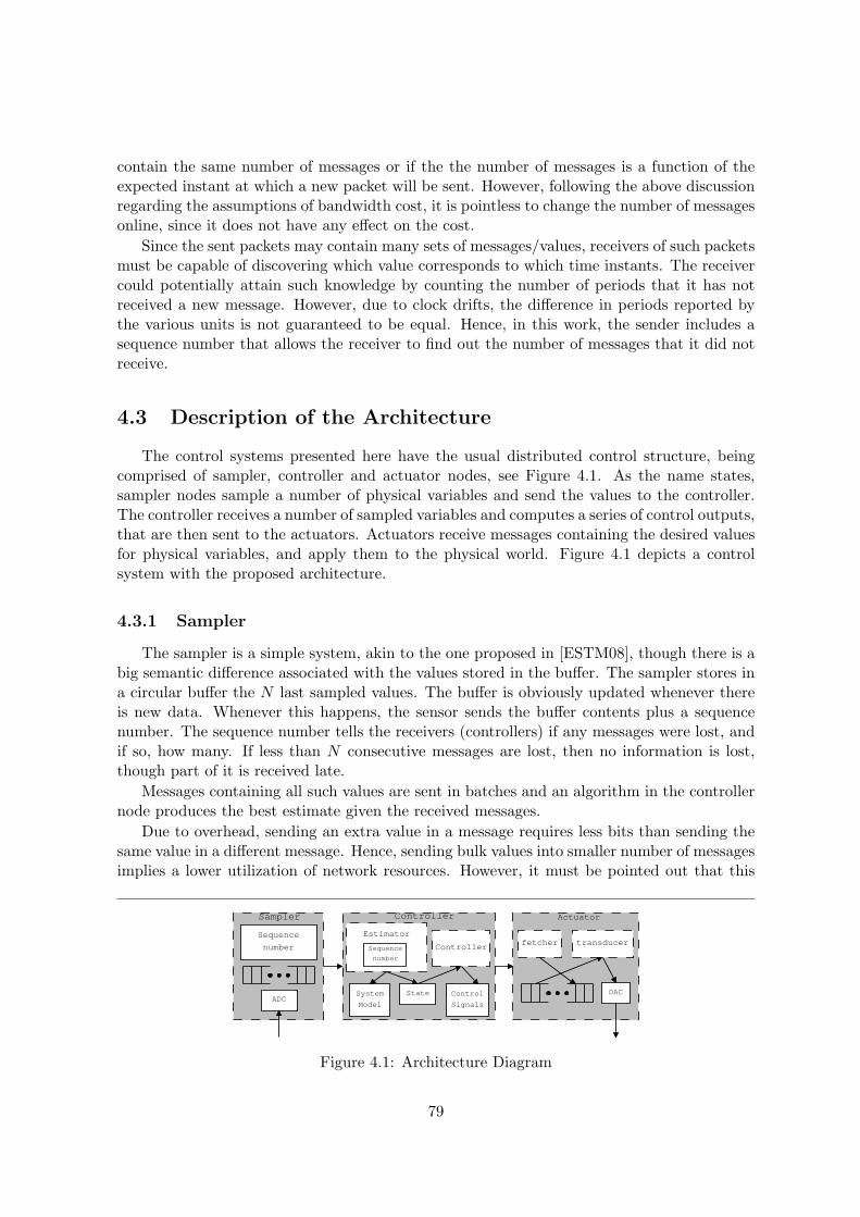
contain the same number of messages or if the the number of messages is a function of theexpected instant at which a new packet will be sent. However, following the above discussionregarding the assumptions of bandwidth cost, it is pointless to change the number of messagesonline, since it does not have any effect on the cost.

Since the sent packets may contain many sets of messages/values, receivers of such packetsmust be capable of discovering which value corresponds to which time instants. The receivercould potentially attain such knowledge by counting the number of periods that it has notreceived a new message. However, due to clock drifts, the difference in periods reported bythe various units is not guaranteed to be equal. Hence, in this work, the sender includes asequence number that allows the receiver to find out the number of messages that it did notreceive.

4.3 Description of the Architecture

The control systems presented here have the usual distributed control structure, beingcomprised of sampler, controller and actuator nodes, see Figure 4.1. As the name states,sampler nodes sample a number of physical variables and send the values to the controller.The controller receives a number of sampled variables and computes a series of control outputs,that are then sent to the actuators. Actuators receive messages containing the desired valuesfor physical variables, and apply them to the physical world. Figure 4.1 depicts a controlsystem with the proposed architecture.

4.3.1 Sampler

The sampler is a simple system, akin to the one proposed in [ESTM08], though there is abig semantic difference associated with the values stored in the buffer. The sampler stores ina circular buffer the N last sampled values. The buffer is obviously updated whenever thereis new data. Whenever this happens, the sensor sends the buffer contents plus a sequencenumber. The sequence number tells the receivers (controllers) if any messages were lost, andif so, how many. If less than N consecutive messages are lost, then no information is lost,though part of it is received late.

Messages containing all such values are sent in batches and an algorithm in the controllernode produces the best estimate given the received messages.

Due to overhead, sending an extra value in a message requires less bits than sending thesame value in a different message. Hence, sending bulk values into smaller number of messagesimplies a lower utilization of network resources. However, it must be pointed out that this

Sequence

number

ADCSystem

Model

State

Estimator

Sequence

number

Controller fetcher transducer

DAC

Sampler Controller Actuator

Control

Signals

Figure 4.1: Architecture Diagram

79

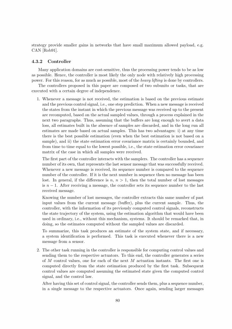
strategy provide smaller gains in networks that have small maximum allowed payload, e.g.CAN [Rob91].

4.3.2 Controller

Many application domains are cost-sensitive, thus the processing power tends to be as lowas possible. Hence, the controller is most likely the only node with relatively high processingpower. For this reason, for as much as possible, most of the heavy lifting is done by controllers.

The controllers proposed in this paper are composed of two subunits or tasks, that areexecuted with a certain degree of independence.

1. Whenever a message is not received, the estimation is based on the previous estimateand the previous control signal, i.e., one step prediction. When a new message is receivedthe states from the instant in which the previous message was received up to the presentare recomputed, based on the actual sampled values, through a process explained in thenext two paragraphs. Thus, assuming that the buffers are long enough to avert a dataloss, all estimates built in the absence of samples are discarded, and in the long run allestimates are made based on actual samples. This has two advantages: i) at any timethere is the best possible estimation (even when the best estimation is not based on asample), and ii) the state estimation error covariance matrix is certainly bounded, andfrom time to time equal to the lowest possible, i.e., the state estimation error covariancematrix of the case in which all samples were received.

The first part of the controller interacts with the samplers. The controller has a sequencenumber of its own, that represents the last sensor message that was successfully received.Whenever a new message is received, its sequence number is compared to the sequencenumber of the controller. If it is the next number in sequence then no message has beenlost. In general, if the difference is n, n > 1, then the total number of lost messagesis n− 1. After receiving a message, the controller sets its sequence number to the lastreceived message.

Knowing the number of lost messages, the controller extracts this same number of pastinput values from the current message (buffer), plus the current sample. Thus, thecontroller, with the information of its previously computed control signals, reconstructsthe state trajectory of the system, using the estimation algorithm that would have beenused in ordinary, i.e., without this mechanism, systems. It should be remarked that, indoing, so the estimates computed without the sampled values are discarded.

To summarize, this task produces an estimate of the system state, and if necessary,a system identification is performed. This task is executed whenever there is a newmessage from a sensor.

2. The other task running in the controller is responsible for computing control values andsending them to the respective actuators. To this end, the controller generates a seriesof M control values, one for each of the next M actuation instants. The first one iscomputed directly from the state estimation produced by the first task. Subsequentcontrol values are computed assuming the estimated state given the computed controlsignal, and the control law.

After having this set of control signal, the controller sends them, plus a sequence number,in a single message to the respective actuators. Once again, sending larger messages

80

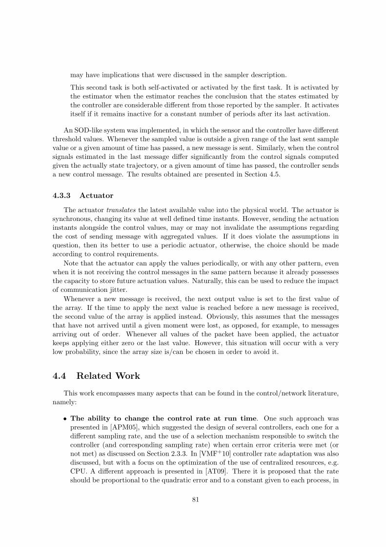
may have implications that were discussed in the sampler description.

This second task is both self-activated or activated by the first task. It is activated bythe estimator when the estimator reaches the conclusion that the states estimated bythe controller are considerable different from those reported by the sampler. It activatesitself if it remains inactive for a constant number of periods after its last activation.

An SOD-like system was implemented, in which the sensor and the controller have differentthreshold values. Whenever the sampled value is outside a given range of the last sent samplevalue or a given amount of time has passed, a new message is sent. Similarly, when the controlsignals estimated in the last message differ significantly from the control signals computedgiven the actually state trajectory, or a given amount of time has passed, the controller sendsa new control message. The results obtained are presented in Section 4.5.

4.3.3 Actuator

The actuator translates the latest available value into the physical world. The actuator issynchronous, changing its value at well defined time instants. However, sending the actuationinstants alongside the control values, may or may not invalidate the assumptions regardingthe cost of sending message with aggregated values. If it does violate the assumptions inquestion, then its better to use a periodic actuator, otherwise, the choice should be madeaccording to control requirements.

Note that the actuator can apply the values periodically, or with any other pattern, evenwhen it is not receiving the control messages in the same pattern because it already possessesthe capacity to store future actuation values. Naturally, this can be used to reduce the impactof communication jitter.

Whenever a new message is received, the next output value is set to the first value ofthe array. If the time to apply the next value is reached before a new message is received,the second value of the array is applied instead. Obviously, this assumes that the messagesthat have not arrived until a given moment were lost, as opposed, for example, to messagesarriving out of order. Whenever all values of the packet have been applied, the actuatorkeeps applying either zero or the last value. However, this situation will occur with a verylow probability, since the array size is/can be chosen in order to avoid it.

4.4 Related Work

This work encompasses many aspects that can be found in the control/network literature,namely:

• The ability to change the control rate at run time. One such approach waspresented in [APM05], which suggested the design of several controllers, each one for adifferent sampling rate, and the use of a selection mechanism responsible to switch thecontroller (and corresponding sampling rate) when certain error criteria were met (ornot met) as discussed on Section 2.3.3. In [VMF+10] controller rate adaptation was alsodiscussed, but with a focus on the optimization of the use of centralized resources, e.g.CPU. A different approach is presented in [AT09]. There it is proposed that the rateshould be proportional to the quadratic error and to a constant given to each process, in

81

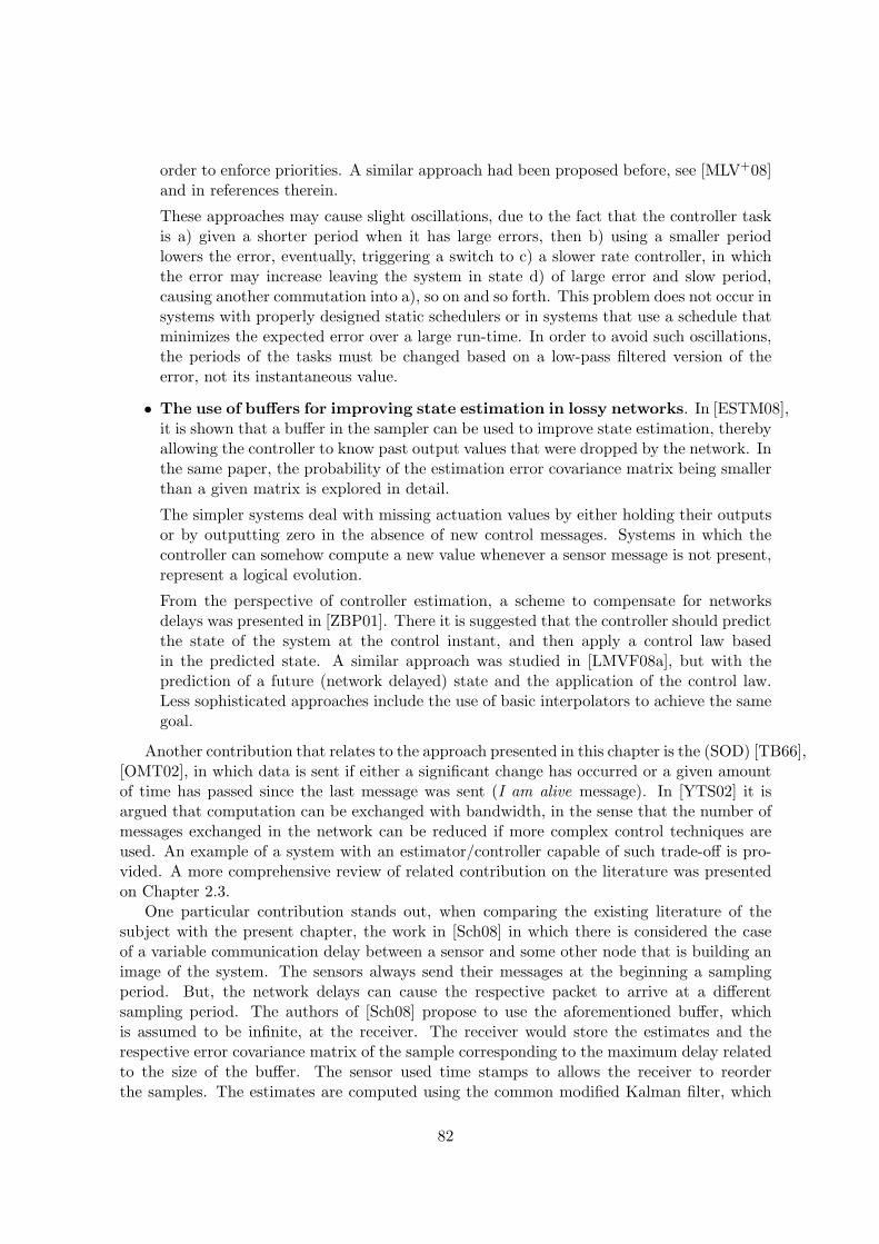
order to enforce priorities. A similar approach had been proposed before, see [MLV+08]and in references therein.

These approaches may cause slight oscillations, due to the fact that the controller taskis a) given a shorter period when it has large errors, then b) using a smaller periodlowers the error, eventually, triggering a switch to c) a slower rate controller, in whichthe error may increase leaving the system in state d) of large error and slow period,causing another commutation into a), so on and so forth. This problem does not occur insystems with properly designed static schedulers or in systems that use a schedule thatminimizes the expected error over a large run-time. In order to avoid such oscillations,the periods of the tasks must be changed based on a low-pass filtered version of theerror, not its instantaneous value.

• The use of buffers for improving state estimation in lossy networks. In [ESTM08],it is shown that a buffer in the sampler can be used to improve state estimation, therebyallowing the controller to know past output values that were dropped by the network. Inthe same paper, the probability of the estimation error covariance matrix being smallerthan a given matrix is explored in detail.

The simpler systems deal with missing actuation values by either holding their outputsor by outputting zero in the absence of new control messages. Systems in which thecontroller can somehow compute a new value whenever a sensor message is not present,represent a logical evolution.

From the perspective of controller estimation, a scheme to compensate for networksdelays was presented in [ZBP01]. There it is suggested that the controller should predictthe state of the system at the control instant, and then apply a control law basedin the predicted state. A similar approach was studied in [LMVF08a], but with theprediction of a future (network delayed) state and the application of the control law.Less sophisticated approaches include the use of basic interpolators to achieve the samegoal.

Another contribution that relates to the approach presented in this chapter is the (SOD) [TB66],[OMT02], in which data is sent if either a significant change has occurred or a given amountof time has passed since the last message was sent (I am alive message). In [YTS02] it isargued that computation can be exchanged with bandwidth, in the sense that the number ofmessages exchanged in the network can be reduced if more complex control techniques areused. An example of a system with an estimator/controller capable of such trade-off is pro-vided. A more comprehensive review of related contribution on the literature was presentedon Chapter 2.3.

One particular contribution stands out, when comparing the existing literature of thesubject with the present chapter, the work in [Sch08] in which there is considered the caseof a variable communication delay between a sensor and some other node that is building animage of the system. The sensors always send their messages at the beginning a samplingperiod. But, the network delays can cause the respective packet to arrive at a differentsampling period. The authors of [Sch08] propose to use the aforementioned buffer, whichis assumed to be infinite, at the receiver. The receiver would store the estimates and therespective error covariance matrix of the sample corresponding to the maximum delay relatedto the size of the buffer. The sensor used time stamps to allows the receiver to reorderthe samples. The estimates are computed using the common modified Kalman filter, which

82

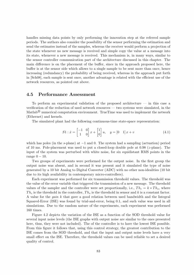
handles missing data points by only performing the innovation step at the referred sampleperiods. The authors also consider the possibility of the sensor performing the estimation andsend the estimates instead of the samples, whereas the receiver would perform a projection ofthe state whenever no new message is received and simple copy the value at a message intoits state, whenever a new message is received. This mechanism is, in many ways, similar tothe sensor controller communication part of the architecture discussed in this chapter. Themain difference is on the placement of the buffer, since in the approach proposed here, thebuffer is at the sensor side which allows to a single sample to be sent more than once, henceincreasing (redundancy) the probability of being received, whereas in the approach put forthin [Sch08], each sample is sent once, another advantage is related with the efficient use of thenetwork resources, as pointed out above.

4.5 Performance Assessment

To perform an experimental validation of the proposed architecture — in this case averification of the reduction of used network resources — two systems were simulated, in theMatlab R⃝ numerical computation environment. TrueTime was used to implement the network(Ethernet) and kernels.

The simulated plant had the following continuous-time state-space representation:

S1 : x =

[−1 01 0

]x+

[10

]u, y = [0 1]x+ v (4.1)

which has poles (in the s-plane) at −1 and 0. The system had a sampling (actuation) periodof 10 ms. Pole-placement was used to put a closed-loop double pole at 0.98 (z-plane). Theinput of the system was perturbed with white noise, for six equidistant RMS points in therange 0− 10.

Two groups of experiments were performed for the output noise. In the first group theoutput noise was absent, and in second it was present and it simulated the type of noisegenerated by a 10 bit Analog to Digital Converter (ADC) with no other non-idealities (10 bitdue to its high availability in contemporary micro-controllers).

Each experiment was performed for six transmission threshold values. The threshold wasthe value of the error variable that triggered the transmission of a new message. The thresholdvalues of the sampler and the controller were set proportionally, i.e., Thc = k ∗ Ths, whereThc is the threshold in the controller, Ths is the threshold in sensor and k is a constant factor.A value for the gain k that gave a good relation between used bandwidth and the IntegralSquared-Error (ISE) was found by trial-and-error, being 0.1, and such value was used in allsimulations. Due to the random nature of the experiments, each experiment was performed160 times.

Figure 4.2 depicts the variation of the ISE as a function of the SOD threshold value forseveral input noise levels (the ISE graphs with output noise are similar to the ones presentedhere, thus, they were not included). The of the controller is to have the lowest ISE possible.From this figure it follows that, using this control strategy, the greatest contribution to theISE comes from the SOD threshold, and that the input and output noise levels have a verysmall effect on the ISE. Therefore, the threshold values can be used reliable to set a desiredquality of control.

83

0 0.2 0.4 0.6 0.8 10

200

400

600

800

1000

1200

1400

1600

1800

ISE

threshold value

noisein

=0.0

noisein

=2.0

noisein

=4.0

noisein

=6.0

noisein

=8.0

noisein

=10.0

Figure 4.2: ISE versus threshold for several noise values

The next simulation results show the influence of the noise level and threshold on theamount of bandwidth that is saved by this architecture. Note that in systems without thepresented architecture, the bandwidth savings are, by definition, zero.

Figures 4.3 show a series of bandwidth measurements. More precisely, they show thesaved bandwidth in percentage, which is computed as:

sb = 100× bstandard − busedbstandard

, (4.2)

where bused is the bandwidth that was measured in the simulation and bstandard is the band-width used by a standard controller, under similar systems and networks.

The first set of graphs (up-left) shows that the saved bandwidth tends to 87.5% when thethreshold values grow unboundedly. This happens because the messages are scheduled to betransmitted with a periodicity of N (as described before), even when the thresholds are notreached. Thus, when the threshold is significantly larger than the error in the signals, 1 outof N messages is sent. Therefore, the saved bandwidth tends to 100 × (N − 1)/N percent.In this case, N = 8 (thus converging to 87.5%). Since Ethernet was used, a message with 8blocks of 2 bytes is well within the maximum payload of 1500 bytes, even when comparedwith the minimum payload, which is of 46 bytes.

On a similar experiment (up-left) done with ADC reading error, the transmission ratewas limited by the ADC noise, i.e, its effects were enough to trigger a transmission (soonerthan the effects of the input noise alone). Hence, the saved bandwidth was less sensitive tothe input noise.

The controller actuator transmission without ADC reading errors — top right — is similarto the sensor-actuator counterpart. However, in the presence of ADC reading errors — bottomleft — there is no significant qualitative difference, mostly because those errors got filteredout due to the higher rate at which the sensor send its messages. The bottom right figuredepicts the controller to actuator case, in the presence of ADC noise.

Not all messages sent from the sensor to controller triggered a message from the controllerto the actuator. If the controller notes that the new messages do not change significantly itsstate estimate, and consequently its control outputs, no new messages will be sent. That isthe primarily reason why the two rightmost graphs of Figure 4.3 are rather similar.

84

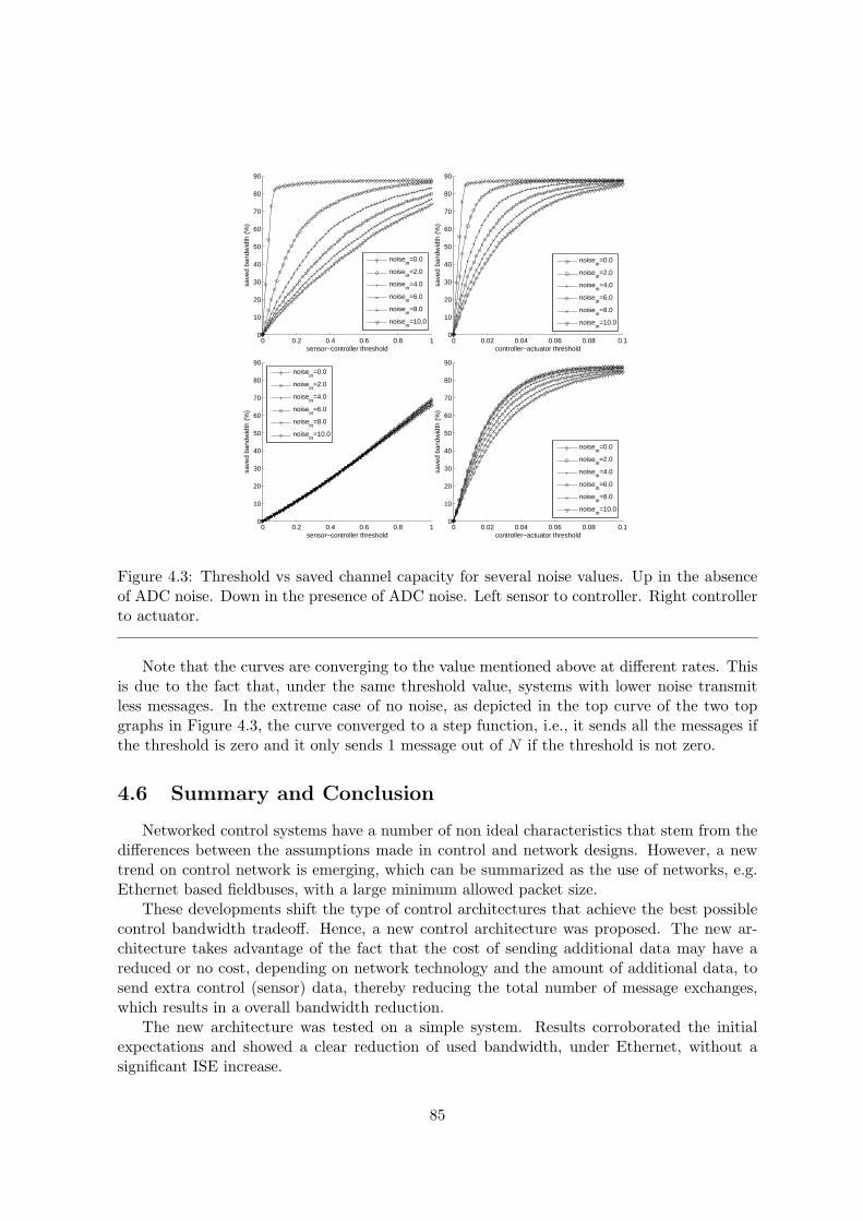
0 0.2 0.4 0.6 0.8 10

10

20

30

40

50

60

70

80

90

save

d ba

ndw

idth

(%

)

sensor−controller threshold

noisein

=0.0

noisein

=2.0

noisein

=4.0

noisein

=6.0

noisein

=8.0

noisein

=10.0

0 0.02 0.04 0.06 0.08 0.10

10

20

30

40

50

60

70

80

90

save

d ba

ndw

idth

(%

)

controller−actuator threshold

noisein

=0.0

noisein

=2.0

noisein

=4.0

noisein

=6.0

noisein

=8.0

noisein

=10.0

0 0.2 0.4 0.6 0.8 10

10

20

30

40

50

60

70

80

90

save

d ba

ndw

idth

(%

)

sensor−controller threshold

noise

in=0.0

noisein

=2.0

noisein

=4.0

noisein

=6.0

noisein

=8.0

noisein

=10.0

0 0.02 0.04 0.06 0.08 0.10

10

20

30

40

50

60

70

80

90

save

d ba

ndw

idth

(%

)

controller−actuator threshold

noisein

=0.0

noisein

=2.0

noisein

=4.0

noisein

=6.0

noisein

=8.0

noisein

=10.0

Figure 4.3: Threshold vs saved channel capacity for several noise values. Up in the absenceof ADC noise. Down in the presence of ADC noise. Left sensor to controller. Right controllerto actuator.

Note that the curves are converging to the value mentioned above at different rates. Thisis due to the fact that, under the same threshold value, systems with lower noise transmitless messages. In the extreme case of no noise, as depicted in the top curve of the two topgraphs in Figure 4.3, the curve converged to a step function, i.e., it sends all the messages ifthe threshold is zero and it only sends 1 message out of N if the threshold is not zero.

4.6 Summary and Conclusion

Networked control systems have a number of non ideal characteristics that stem from thedifferences between the assumptions made in control and network designs. However, a newtrend on control network is emerging, which can be summarized as the use of networks, e.g.Ethernet based fieldbuses, with a large minimum allowed packet size.

These developments shift the type of control architectures that achieve the best possiblecontrol bandwidth tradeoff. Hence, a new control architecture was proposed. The new ar-chitecture takes advantage of the fact that the cost of sending additional data may have areduced or no cost, depending on network technology and the amount of additional data, tosend extra control (sensor) data, thereby reducing the total number of message exchanges,which results in a overall bandwidth reduction.

The new architecture was tested on a simple system. Results corroborated the initialexpectations and showed a clear reduction of used bandwidth, under Ethernet, without asignificant ISE increase.

85

Chapter 5

Control over Lossy Networks

5.1 Introduction

In the previous chapter, it was shown that many networks used in control (in particularEthernet), have a minimum data length that allows for the transmission of extra control(sensor) data at small or no cost. However, such extra sent data was primarily used forreducing the overall bandwidth requirements, which was achieved by reducing the number oftransmitted messages.

Even though during the last four decades the average processing and communication ca-pabilities of the nodes employed in distributed control systems have increased steadily, thesesystems are frequently deployed in harsh environments, being subject to strong electromag-netic interference, noisy power supplies, mechanical vibration, among other perturbations.Thus, despite all aforementioned advances, communications are still affected by non-negligibleerror-rates. The move towards wireless media, currently observed in many application areas,exacerbates this problem. Obviously, the performance of control applications supported bythis kind of communication infrastructure can be severely deteriorated. Thus, to achieve anadequate quality of control, it is necessary to develop a control framework that takes intoaccount the effects of packet losses in control and estimation.

The main drive behind this chapter is to investigate the possibility of using the type ofcontrol architecture developed in the previous chapter to lessen the effects of packet drops.Evidently, this is a problem of estimation and control in networks with packet drops.

Over the last few years, the problem of optimal estimation and control over lossy networkshas been studied in detail. However, unlike the approach in this Thesis, most of such worksassume that in the absence of a new actuation value, the actuator either applies zero or theprevious applied value. Some other extensions have been proposed, but even though they arepresented as different approaches to the same problem, they present similar performance.

In this chapter it is argued that these methods are not optimal. Moreover, a new approachin which the controller sends a number of predictions of future actuation values, which areapplied when the actuator does not receive a new message, is presented. Under this newapproach it is shown that the controller/estimator herein presented performs equal to or betterthan any previously introduced controller, the equality being verified only in the absence ofcommunication errors. A modified Kalman filter as well as a specific optimal controllerfor this novel actuation model are also presented. For the sake of simplicity and withoutprejudice to the assumption of a fully distributed architecture, this chapter assumes that batch

87

fetcher transducerkV kuz

kuk

0

kz

Z-1

ku

b) c)a)

Figure 5.1: Types of output strategies. a) output zero, b) hold, c) proposed approach.

transmissions occurs only between the controller and the actuator. The sensor controller casecan be studied either in a similar way or by, for example, applying the control/estimationduality.

Depending on the existence or not of explicit acknowledgment signals, communicationprotocols are usually classified into TCP-like and UDP-like categories, respectively [IYB06].Since it is assumed a fully-distributed architecture, under TCP-like protocols the controllerreceives an acknowledgment from the actuator signaling the correct reception of the lastactuation value. Therefore, in TCP like protocols, whenever a state-estimation is performed,the estimator has perfect knowledge of the inputs of the system. However, under UDP-likeprotocols, there are no such acknowledgments, thus the estimator cannot know which inputwas used in the previous actuation instant.

Such lack of information, under UDP-like protocols, regarding the correct reception ofmessages by the actuator renders the estimation error covariance matrix a function of theinput, thus leading to a complex (i.e., non-quadratic) optimization problem, which has noknown optimal solution. A more in depth discussion of these type of problems can be found,for example, in [SSF+07]. The use of TCP-like protocols suffers less from this ailments.However, it requires acknowledgments that, a) are also sent over a lossy network, and thereforeare themselves subject to errors b) increase the transmission error probability c) increase thenetwork load and complexity of the communication stacks.

Note, that the terms TCP-like and UDP-like do not refer to the protocols that are usedin the Internet Protocol Stack (IP), i.e., OSI level 4. Instead, they are simply used to denoteprotocols whether it is possible to the sender to know if the message was correctly transmitted.

The literature presents two main strategies to cope with missing actuation data. In thefirst one, called output zero, if there is no new message the actuator applies zero, shown inFigure 5.1 a). In the second one, called hold, in the absence of a new message the actuatorapplies the previous value (Figure 5.1 b)). This Thesis argues that the best option is to usean estimation of the control value given the set of previous control and output values (Figure5.1 c)). This scheme provides a simple and optimal realization. The control wise optimality isproven in this chapter, whereas the bandwidth wise optimality is assumed from the networkassumptions.

This chapter also shows that for TCP-like protocols the separation principle holds, i.e.,the error covariance matrix is independent of the controller gain, while for UDP-like protocolsthe separation principle does not hold in general, though, as will be shown, for the class ofcontrollers presented in this chapter, the estimation auto-covariance matrix is independentof the state. Therefore, for the controller presented herein, both for TCP and for UDP-likeprotocols, the optimal estimator is independent of the optimal controller.

88

5.2 Related Work

The subject of estimation and control over lossy networks is relatively old. The first ap-pearances of it in the literature try to find a correspondence between the Shannon informationtheory [Sha48] and control theory. More specifically, they tried to answer the question: whatis the smallest bit-rate necessary to stabilize a given system or, equivalently, what is the maxi-mum transmission error rate that a network can have that ensures the stability of the system?Furthermore, which techniques (architecture) achieve this threshold? is a question that, tothe best of the author’s knowledge, has not yet been addressed by the scientific communityand it is hopped that our work aids in its response. A number of early attempts to answerthe first question, i.e., the connection with Shannon’s information theory, are presented inthe survey [HOV02, HNX07].

In [As03] the authors attempt to extend the classical theory of optimal control [Ber07,KJA97]. However, they conclude that the separation principle, which allows a simplification ofthe results, does not hold in the general case. However, other simpler results are shown, suchas, that a system is stable if the independent and identically distributed (i.i.d.) variables thatdescribe the error rate (α) verify α < [max |λ(A)|]−2, assuming that the system is unstable,where λ(X) is the set of all eigenvalues of the matrix X and A is the discrete-time state-transition matrix. Similar claims are made in [HY07].

In [SSF+07] it is made a more in-depth study of such issues, formally presenting the UDPand TCP-like protocol cases. TCP-like protocols are more malleable to the existing optimalcontrol theory, whereas UDP-like protocols, under the assumptions made therein (outputzero) yields a complex optimization problem, since the estimation error covariance matrix atany given time step will depend on previous control values. In [SSF+07] it is also shown that,under their assumptions, TCP-like protocols have an error-rate similar to the one found inthe previous papers, but UDP-like protocols have lower error-rate bounds that guaranteesstability.

Another related development is given in [HY08], in which state information is sent in morethan one packet. This fragmentation is done primarily in an attempt to reduce the impact ofpacket losses, since loosing a packet with a significant large number of state variables wouldbe worst than loosing one packet with only one variable.

In [KKH+08] it is taken a radically different approach, i.e., passive networks — networksthat can be implemented using only passive elements — are used as a mean to provide jitterimmunity for the controlled system. However, no reasons to believe that passive networksare more immune to jitter are presented, and no mechanism to design passive controllersto achieve certain metrics, e.g. state-tracking or input tracking under noisy conditions, areprovided.

In [GSC08] the authors introduce a new concept, i.e., the packet acknowledgment is alsoprobabilistic. By varying the probability of an acknowledgment, it is possible to go from noacknowledgment (UDP-like protocols) through a grey zone up to the situation in which thereis an acknowledgment with probability one (TCP-like protocols). Therefore, in a certain way,they extended the notion of UDP-like versus TCP-like protocols. Even though it is a veryactive research topic, this extension was not considered in this Thesis because: 1) the authoris not aware of any network protocols that support such an extension, 2) it is normally dealtwith as in the case of UDP-like protocols, i.e., the separation principle does not hold, hence,classical minimization techniques cannot be applied, therefore, the extension is not actuallysolved.

89

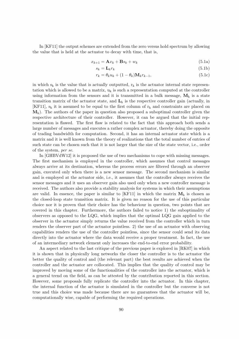
In [KF11] the output schemes are extended from the zero versus hold spectrum by allowingthe value that is held at the actuator to decay with time, that is,

xk+1 = Axk +Bsk + wk (5.1a)

sk = Lkrk (5.1b)

rk = θkuk + (1− θk)Mkrk−1, (5.1c)

in which sk is the value that is actually outputted, rk is the actuator internal state represen-tation which is allowed to be a matrix, uk is such a representation computed at the controllerusing information from the sensors and it is transmitted in a bulk message, Mk is a statetransition matrix of the actuator state, and Lk is the respective controller gain (actually, in[KF11], sk it is assumed to be equal to the first column of rk and constraints are placed onMk). The authors of the paper in question also proposed a suboptimal controller given therespective architecture of their controller. However, it can be argued that the initial rep-resentation is flawed. The first flaw is related to the fact that this approach both sends alarge number of messages and executes a rather complex actuator, thereby doing the oppositeof trading bandwidth for computation. Second, it has an internal actuator state which is amatrix and it is well known from the theory of realizations that the total number of entries ofsuch state can be chosen such that it is not larger that the size of the state vector, i.e., orderof the system, per se.

In [GHBVdW12] it is proposed the use of two mechanisms to cope with missing messages.The first mechanism is employed in the controller, which assumes that control messagesalways arrive at its destination, whereas the process errors are filtered through an observergain, executed only when there is a new sensor message. The second mechanism is similarand is employed at the actuator side, i.e., it assumes that the controller always receives thesensor messages and it uses an observer gain also used only when a new controller message isreceived. The authors also provide a stability analysis for systems in which their assumptionsare valid. In essence, the paper is similar to [KF11] in which the matrix Mk is chosen asthe closed-loop state transition matrix. It is given no reason for the use of this particularchoice nor it is proven that their choice has the behaviour in question, two points that arecovered in this chapter. Furthermore, the authors failed to notice 1) the suboptimality ofobservers as opposed to the LQG, which implies that the optimal LQG gain applied to theobserver in the actuator simply returns the value received from the controller which in turnrenders the observer part of the actuator pointless. 2) the use of an actuator with observingcapabilities renders the use of the controller pointless, since the sensor could send its datadirectly into the actuator where the data would receive a proper treatment. In fact, the useof an intermediary network element only increases the end-to-end error probability.

An aspect related to the last critique of the previous paper is explored in [RK07] in whichit is shown that in physically long networks the closer the controller is to the actuator thebetter the quality of control and (the relevant part) the best results are achieved when thecontroller and the actuator are collocated. This implies that the quality of control may beimproved by moving some of the functionalities of the controller into the actuator, which isa general trend on the field, as can be attested by the contribution reported in this section.However, some proposals fully replicate the controller into the actuator. In this chapter,the internal function of the actuator is simulated in the controller but the converse is nottrue and this choice was made because there are no guarantees that the actuator will be,computationally wise, capable of performing the required operations.

90

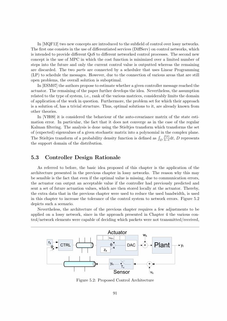
In [MQF12] two new concepts are introduced to the subfield of control over lossy networks.The first one consists in the use of differentiated services (DiffServ) on control networks, whichis intended to provide different QoS to different networked control processes. The second newconcept is the use of MPC in which the cost function is minimized over a limited number ofsteps into the future and only the current control value is outputted whereas the remainingare discarded. The two parts are connected by a scheduler that uses Linear Programming(LP) to schedule the messages. However, due to the connection of various areas that are stillopen problems, the overall solution is suboptimal.

In [ESM07] the authors propose to estimate whether a given controller message reached theactuator. The remaining of the paper further develops the idea. Nevertheless, the assumptionrelated to the type of system, i.e., rank of the various matrices, considerably limits the domainof application of the work in question. Furthermore, the problem set for which their approachis a solution of, has a trivial structure. Thus, optimal solutions to it, are already known fromother theories.

In [VH09] it is considered the behaviour of the auto-covariance matrix of the state esti-mation error. In particular, the fact that it does not converge as in the case of the regularKalman filtering. The analysis is done using the Stieltjes transform which transforms the setof (expected) eigenvalues of a given stochastic matrix into a polynomial in the complex plane.

The Stieltjes transform of a probability density function is defined as∫D

f(t)λ−tdt, D represents

the support domain of the distribution.

5.3 Controller Design Rationale

As referred to before, the basic idea proposed of this chapter is the application of thearchitecture presented in the previous chapter in lossy networks. The reason why this maybe sensible is the fact that even if the optimal value is missing, due to communication errors,the actuator can output an acceptable value if the controller had previously predicted andsent a set of future actuation values, which are then stored locally at the actuator. Thereby,the extra data that in the previous chapter were used to reduce the used bandwidth, is usedin this chapter to increase the tolerance of the control system to network errors. Figure 5.2depicts such a scenario.

Nevertheless, the architecture of the previous chapter requires a few adjustments to beapplied on a lossy network, since in the approach presented in Chapter 4 the various con-trol/network elements were capable of deciding which packets were not transmitted/received,

+ PlantCTRL

+

rkφ

Tsyk

wk

vk

ytDACzk

θ

uk|k-j

Actuator

Sensor

Figure 5.2: Proposed Control Architecture

91

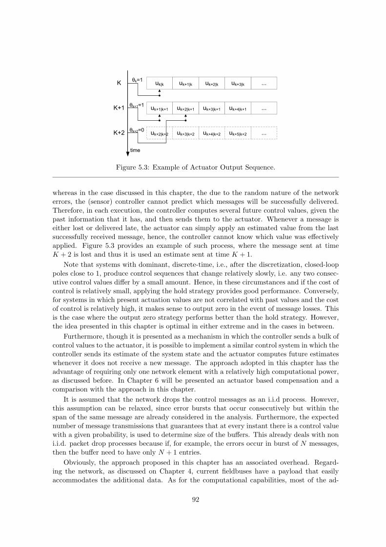
time

θk+2=0

θk+1=1

θk=1 uk|k

uk+1|k+1

uk+2|k+2

uk+1|kK

uk+3|k+1 uk+4|k+1uk+2|k+1

...

...

uk+5|k+2uk+4|k+2uk+3|k+2

uk+3|kuk+2|k

K+1

K+2 ...

Figure 5.3: Example of Actuator Output Sequence.

whereas in the case discussed in this chapter, the due to the random nature of the networkerrors, the (sensor) controller cannot predict which messages will be successfully delivered.Therefore, in each execution, the controller computes several future control values, given thepast information that it has, and then sends them to the actuator. Whenever a message iseither lost or delivered late, the actuator can simply apply an estimated value from the lastsuccessfully received message, hence, the controller cannot know which value was effectivelyapplied. Figure 5.3 provides an example of such process, where the message sent at timeK + 2 is lost and thus it is used an estimate sent at time K + 1.

Note that systems with dominant, discrete-time, i.e., after the discretization, closed-looppoles close to 1, produce control sequences that change relatively slowly, i.e. any two consec-utive control values differ by a small amount. Hence, in these circumstances and if the cost ofcontrol is relatively small, applying the hold strategy provides good performance. Conversely,for systems in which present actuation values are not correlated with past values and the costof control is relatively high, it makes sense to output zero in the event of message losses. Thisis the case where the output zero strategy performs better than the hold strategy. However,the idea presented in this chapter is optimal in either extreme and in the cases in between.

Furthermore, though it is presented as a mechanism in which the controller sends a bulk ofcontrol values to the actuator, it is possible to implement a similar control system in which thecontroller sends its estimate of the system state and the actuator computes future estimateswhenever it does not receive a new message. The approach adopted in this chapter has theadvantage of requiring only one network element with a relatively high computational power,as discussed before. In Chapter 6 will be presented an actuator based compensation and acomparison with the approach in this chapter.

It is assumed that the network drops the control messages as an i.i.d process. However,this assumption can be relaxed, since error bursts that occur consecutively but within thespan of the same message are already considered in the analysis. Furthermore, the expectednumber of message transmissions that guarantees that at every instant there is a control valuewith a given probability, is used to determine size of the buffers. This already deals with noni.i.d. packet drop processes because if, for example, the errors occur in burst of N messages,then the buffer need to have only N + 1 entries.

Obviously, the approach proposed in this chapter has an associated overhead. Regard-ing the network, as discussed on Chapter 4, current fieldbuses have a payload that easilyaccommodates the additional data. As for the computational capabilities, most of the ad-

92

ditional burden is put on the controller node, which normally is a node with relatively highcomputational capabilities.

5.4 Problem Statement and Solution

Consider a fully distributed system, as depicted in Figure 5.2, with linear dynamics.Notwithstanding its linear dynamics, there are some differences with the previous chapterthat makes it is necessary to redefine some of its variables and to introduce others. Thesystem under this architecture has the state-space representation:

xk+1 = Axk +Bzk + wk (5.2a)

yk = Cxk + vk, (5.2b)

where x is the state variable, z is the control value that is applied by the actuator, w is theinput noise, y is the output as sampled by the sampler, v is the output noise, and k is thesample index. Note that the variable u, that appeared in previous chapters, is the controlvalue as computed by the controller, as opposed to z, the value applied by the actuator. A,Band C are the state transition, input and output matrices, respectively. Let xk|k−j be theoptimal estimate of xk given all the information known at instant k − j.

Let there also be defined

Pk|k−j = E[(xk|k−j − xk) (xk|k−j − xk)

′] (5.3a)

E[[wk vk][wi vi]

′] = [Q 00 R

]δki, (5.3b)

where Pk|k−j is the auto-covariance matrix of the estimation of xk given all the informationreceived up to the instant k−j. Q and R are the input and output error covariance matrices,respectively. These last two matrices are not necessarily constant. However, since this factdoes not have a direct impact in the results presented herein, it will be assumed that they areconstant. δki is the Kronecker delta which is 1 if k = i and 0 otherwise. It is also assumedthat w and v are uncorrelated white Gaussian noise sequences.

Considering a linear controller and that the certainty equivalence principle holds, as willbe shown in a subsequent section, each possible output of the controller can be written as:

uk|k−i = −Lkxk|k−i (5.4)

in which xk|k−i is the state estimation as defined above, Lk is the controller gain matrix at

the kth step and uk|k−i is the value that the controller expected at instant k − i to be theoptimal control value at instant k.

Due to the fact that the architecture considered in this chapter is fully distributed, com-munication errors may happen both between the sensor and the controller and between thecontroller and the actuator. It is assumed that the underlying communication network pro-vides suitable error correction/detection mechanisms so that messages are either correctlyreceived or discarded. As illustrated in Figure 5.2, transmission errors are modeled by theboolean variables φk (sensor-controller) and θk (controller-actuator), which take the logicalvalue 1 if the transmission is carried out correctly and 0 otherwise. Furthermore, regardingtheir stochastic behavior, it is assumed that these variables are i.i.d. Bernoulli variables, i.e.,Pr(θk = 1) = Pr(φk = 1) = θ and Pr(θk = 0) = Pr(φk = 0) = 1− θ.

93

As stated before, in virtue of the employed architecture, in each period (k − j) the con-troller computes uk−j as well as a set of j future values uk−j+1|k−j uk−j+2|k−j ...uk|k−j.These future values are computed based in the expectation of the system state x at theirrespective application instants. It is important to stress that these estimates are updated bythe controller and sent to the actuator in each controller execution. Therefore, each one ofthe estimated control values uk−i|k−j , i ∈ 0..(j − 1) is applied if and only if its predecessoru(k−i)−1|k−j was also applied. This is so because the correct reception of a message at instant(k −m) replaces all previous estimates in the interval (k −m)...k. This fact significantlysimplifies the computation of uk|k−j .

Under the presented conditions above, the value that is actually used by the actuator atperiod k, i.e., zk, may be different from the value generated by the controller at the sameexecution uk, being equal to:

zk =k∑

j=0

θj

k∏l=j+1

(1− θl)

uk|j (5.5)

The boolean part of the argument of summation is 1 if the jth message was received and allthe future messages up to the instant k were not. Therefore, the whole summation tells 1)what was the last received message and 2) what was the estimate of uk at that time.

Hence, the state in the next step, can be written as

xk+1 = Axk +Bzk + wk (5.6a)

= Axk +B

k∑j=0

θj

k∏l=j+1

(1− θl)

uk|j + wk (5.6b)

in which (5.6b) is a substitution of zk, due to (5.5), into (5.6a); (5.6a) is one of the dynamicequations.

5.4.1 Noise Filtering

As discussed on chapter 2, in centralized control problem, the computation of the stateestimates involves two complementary steps. In the first one, designated innovation, anestimation of the state in the next instant is made, followed by the the computation ofits associated error covariance matrix. The estimates associated with the innovation stepare computed solely based on the dynamic equations, with no information whatsoever ofthe output. The second step, designated correction, consists in a comparison of actualobservations, i.e., the output as for example read by a sensor (with certain error covariancematrices), with the previously made estimations and the computation of new estimations witha lower error covariance matrix. Both of these steps are presented in detail in the followingsections. Since UDP- and TCP-like protocols behave differently, a separate analysis for eachof them is presented.

Innovation

The innovation step is based on Equation (5.6), consisting on the computation of thestate variable at the next instant given the information available prior to the reception of

94

the sample of the instant in question. UDP-like protocols lack acknowledgment mechanisms,therefore the values of θj are unknown on the controller side. Given the type of control thatis proposed, this behavior can be modeled with the help of three new variables, tk, ek and ϵk,defined as follows:

• tk = θkxk|k +(1− θk) (A−BLk−1) tk−1 is the state estimate that results from equation(5.5), representing the state estimation that was (or would have been if the system werecentralized) used when computing the control value that the actuator actually appliedto the environment;

• ek = φk+1

((A−BLk−1)xk−1|k−1 − xk|k

)is the information acquired about the state

variable by performing the kth correction step, being equal to the difference betweenthe uncorrected and corrected state estimation. If no sensor message is received andthereby with no correction, this variable is equal to zero;

• εk is a state variable associated with the input ek, i.e., εk+1 = (A−BLk)εk+φk+1ek+1,where φk+1 is the boolean variable defined above, which models the communicationerrors between the sensor and the controller.

Since t and ε were defined recursively, it is also necessary to define boundary conditions.Given the physical meaning associated with the variables, it is sane to define t0 = x0 andε0 = 0. The first equality follows from the definition by comparing the definitions of t0 andx0. The second equality follows from the fact that at initialization time no corrections havebeen made yet. Note that φk+1ek+1 = ek+1 since whenever φk+1 = ‘0’ there is no updatehence ek+1 = 0, hence the multiplication by φk+1 is redundant, and whenever φk+1 = ‘1’ itis the neutral element of multiplication, therefore, it is always redundant.

Under these assumptions tk = xk|k + (1− θk) εk. The last statement can easily be provenby induction, i.e., the initial value already satisfies the assumption since by definition t0 = x0and ε0 = 0, and the recursion can be verified as follows

tk+1 = θk+1xk+1|k+1 + (1− θk+1) (A−BLk) tk (5.7a)

= θk+1xk+1|k+1 + (1− θk+1) (A−BLk)(xk|k + εk

)(5.7b)

= θk+1xk+1|k+1 + (1− θk+1)[(xk+1|k+1 + φk+1ek+1

)+ (A−BLk) εk

](5.7c)

= xk+1|k+1 + (1− θk) [φk+1ek+1 + (A−BLk) εk] (5.7d)

= xk+1|k+1 + (1− θk) εk+1. (5.7e)

This new set of variables finds its application in the description of the dynamic equationsince the state and the state estimation variables can be written as:

xk+1 = Axk −BLktk + wk (5.8a)

xk+1|k = Axk|k −BLk tk (5.8b)

tk+1 = θxk+1|k + (1− θ) (A−BLk) tk (5.8c)

ek = (A−BLk−1) xk−1|k−1 − xk|k (5.8d)

εk+1 = (A−BLk) εk + φk+1ek+1, (5.8e)

in which Equation (5.8a) follows due to the assumption that tk is the state variable usedto produce zk, i.e., the control value that was actually applied, hence, using the linearity

95

of the controller it follows that tk = −Lkzk, which when substituted on Equation (5.2a)yields Equation (5.8a). Equation (5.8b) follows from Equation (5.8a) because it dictates thebehaviour of the state estimates. Note the introduction of a new variable tk which is anestimate of tk which is the object of Equation (5.8c) in which the equation for the evolutionof tk is laid out. Equation (5.8d) and Equation (5.8e) do similar things to ek and εk+1. Notethat the new εk+1 does not come with an estimation sign, because the previously defined εk+1

was already an estimate.Equation (5.8) implies that ek+1|k = xk+1|k − xk is equal to

ek+1|k = Aek|k − wk −(θ − θk

)BLkεk. (5.9)

The error auto-covariance matrix, i.e., E[ek+1|ke

′k+1|k

], is therefore

Pk+1|k = APk|kA′ +Q+ θ

(1− θ

)BLkεkε

′k (BLk)

′ (5.10)

in which there are no terms in E[ek+1|kε

′k

]despite the correlation of the two variables being

non-zero, because all such terms come multiplied by E[(θ − θk

)]which is zero by (the) defi-

nition (of θ). The past equations fully describe the innovation step under UDP-like protocols.Under TCP-like protocols, it is always known whether or not a message was delivered.

Therefore, even though TCP-like protocols have a similar mechanism (involving ε), the appliedvalue, zk, is always known. For this reason, there is no need to estimate the value that wasapplied by the actuator. This implies that the innovation step is equal to the innovation stepof the standard Kalman Filter, i.e.

xk+1|k = Axk|k +Bzk (5.11a)

Pk+1|k = APk|kA′ +Qk (5.11b)

Correction

The correction step is independent of the type of protocol used to exchange messagesbetween the controller and the actuator, because it depends only of the sensor-controllermessage transfer and at the time of the correction the controller knows whether or not it hasreceived a new sensor message. Note that the notion of UDP vs TCP-like, in this particularscenario ought to be applied to the sensor, since it is the sender of the message, but the sensoris not the network element that is performing the computation. In fact, such element, is thecontroller, which is the one that supposedly sends a message acknowledging the reception ofthe sensor’s message. In any case, the controller always know whether it received the sensormessage at the time of the correction step.

The correction is made only when a sensor message is received, since otherwise there wouldbe no sample to compare the estimates with. For this reason, Kk+1 is multiplied by φk+1.The rest of the correction step is equal to the correction step of a standard Kalman filter, i.e.,

Kk+1 = φk+1Pk+1|kC′ (CPk+1|kC

′ +Rk

)−1(5.12a)

Pk+1|k+1 =(In −Kk+1C

′)Pk+1|k (5.12b)

xk+1|k+1 = xk+1|k +Kk+1

(yk+1 −Cxk+1|k

). (5.12c)

Note that if φk+1 = 0, then Equation (5.12) implies that no correction is made, i.e.,xk+1|k+1 = xk+1|k and Pk+1|k+1 = Pk+1|k.

96

5.4.2 Optimal Control over Lossy Networks — TCP-Like Protocols

Thanks to the existence of controller-actuator acknowledgments, the general principlesbehind the dynamic programming theory, as described in Section 2.3.1, are valid for TCP-like protocols. It is important to notice that in this case: 1) the controller knows the innerstate of the actuator and its inputs, thus, it is able to determine the applied value, 2) once acontroller message is delivered, its respective values will be outputted until the reception of anew controller message, and 3) the certainty equivalence principle is still valid since the errordoes not depend on the control variable and according, for example, to [TBS75] wheneverthis condition is verified, the certainty equivalence is valid. Taking these three observations inconsideration, the computation of new control values under the proposed scheme is no differentthan the computation of such values under classical optimal control, which is presented below.

Let Jk be defined as:

Jk(xk) = x′NWNxN +N−1∑j=k

(x′jWjxj + u′jUjuj) (5.13)

with k and N the limits of the minimization window. Lets also define the value functionVk(x) = x′kPkxk + ck as the usual value function, in which Vk(xk) = minuk

Jk, also known asthe cost-to-go function, as defined in Chapter 2. Then using the Bellman-Hamilton-Jacobitheorem, Vk(xk) can be written as

Vk(x)=x′kWkxk+minuk

(u′kUkuk+(Axk+Buk+wk)

′Pk+1(Axk+Buk+wk)

)+ck+1 (5.14)

At each control iteration, the controller produces a set of values that are assumed to beapplied according to the description provided above. This set of rules, pre-programmed intothe various networked control elements ensures that a given control value is applied only ifthe previous control value was applied, as discussed above.

The reasoning presented in the last paragraph plus the fact that the separation principleholds for TCP-like protocols implies that the minimization can ignore the network side andsimply minimize in order to uk, i.e.

∂Vk(xk)

2∂uk= u′kUk + (Axk +Buk + wk)

′Pk+1B = 0 (5.15)

The last equation was equated to zero because it is known that the minimum is an ex-tremum of Vk(xk). Furthermore, it is solved into (after transposition)

u∗k = −(B′Pk+1B+Uk

)−1B′Pk+1Axk. (5.16)

The previous equation implicitly defines Lk that appears in uk = −Lkxk. The equationdefines the optimal controller in terms of the actual state variable, xk, as opposed to theestimation of the state variable. This is allowed due to the certainty equivalence principlewhich is not broken under TCP-like protocols.

Subtracting an appropriate form of Equation (5.15) from Equation (5.14) yields

Vk(xk)−∂Vk(xk)

2∂ukuk=x′kWkxk+u

′kUkuk+(Axk−BLkxk+wk)

′Pk+1(Axk+wk)+ck+1. (5.17)

97

E [xkw′k] = 0n×n because otherwise the system would either be non-causal in which case wk

would be able to affect at least one state that temporally preceded it, i.e., ∃j≤k : xj = xj(wk),or the system would violate the assumption that wk is a white noise sequence in whichcase a previous perturbation could influence both the current state and the current inputperturbation.

E [xkw′k] = 0 eliminates the cross terms containing such terms from Equation (5.17). Then

a comparison of the terms in the definition of Vk(xk) with Equation (5.17) implies that:

Pk = Wk + (A−BLk)′Pk+1A (5.18a)

ck = ck+1 + trace (QPk+1) (5.18b)

with the boundary conditions PN = WN and cN = 0.

Note that the controller presented above is structural very close to the centralized onethat can be found, for example, in [Kired].

5.4.3 Optimal Control Over Lossy Networks — UDP-Like Protocols

The computation of optimal control values under UDP-like protocols is normally morecomplex than the computation of optimal control values under TCP-like problems. As pointedout in the introduction section, under this type of protocol the separation and certaintyequivalence principles are not guaranteed to hold. Furthermore, when these principles do nothold, the minimization problem, from which the optimal control value stems, is no longerquadratic.

However, in Section 5.4 was shown that ek|k−1 = xk|k−1 − xk is independent of xk even

over UDP-like protocols. This fact implies that Pk|k−1 = E[ek|k−1e

′k|k−1

]must also be

independent of xk. In fact, it is possible to prove that some of the other extended inputstechniques discussed in Section 5.2 also have this property.

Having the above mentioned property is a sufficient condition for the certainty equivalenceprinciple to hold, as shown in [TBS75]. This implies that the optimal controller can be derivedas the classical optimal controller, as shown in the previous subsection.

Nevertheless, the actual control values will be different since they are computed fromdifferent state estimates, which, for example, have different error auto-covariance matrices.

5.5 Simulations and Results

In order to evaluate the validity of the methods proposed in this chapter, two sets ofsimulations were performed. The first set was centered in the validation of the method perse, and to show its benefits when compared to other methods, whereas the second set ofsimulations is a remake of a simulation performed in the paper [SSF+07] which was modifiedin order to include the methods presented herein. Both simulations were made using Matlab R⃝.

The first set of simulations used were performed in a system that had the following discrete-

98

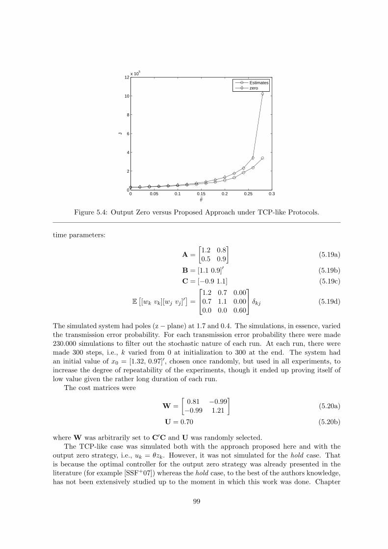
0 0.05 0.1 0.15 0.2 0.25 0.30

2

4

6

8

10

12x 10

5

θ

J

Estimateszero

Figure 5.4: Output Zero versus Proposed Approach under TCP-like Protocols.

time parameters:

A =

[1.2 0.80.5 0.9

](5.19a)

B = [1.1 0.9]′ (5.19b)

C = [−0.9 1.1] (5.19c)

E[[wk vk][wj vj ]

′] =1.2 0.7 0.000.7 1.1 0.000.0 0.0 0.60

δkj (5.19d)

The simulated system had poles (z− plane) at 1.7 and 0.4. The simulations, in essence, variedthe transmission error probability. For each transmission error probability there were made230.000 simulations to filter out the stochastic nature of each run. At each run, there weremade 300 steps, i.e., k varied from 0 at initialization to 300 at the end. The system hadan initial value of x0 = [1.32, 0.97]′, chosen once randomly, but used in all experiments, toincrease the degree of repeatability of the experiments, though it ended up proving itself oflow value given the rather long duration of each run.

The cost matrices were

W =

[0.81 −0.99−0.99 1.21

](5.20a)

U = 0.70 (5.20b)

where W was arbitrarily set to C′C and U was randomly selected.The TCP-like case was simulated both with the approach proposed here and with the

output zero strategy, i.e., uk = θzk. However, it was not simulated for the hold case. Thatis because the optimal controller for the output zero strategy was already presented in theliterature (for example [SSF+07]) whereas the hold case, to the best of the authors knowledge,has not been extensively studied up to the moment in which this work was done. Chapter

99

6 will address this matter. The UDP-like protocol was simulated only with the solutionprovided in this paper, for reasons similar to the previous one, i.e., other output methods donot provide any clue on optimal control values.

Figure 5.4 compares the behaviour of the output zero strategy with the strategy proposedherein, for TCP-like protocols. The graph is shown with a (natural) logarithmic y-axis dueto the rather wide range of total cost J . At low error probabilities the performance ofboth strategies is indistinguishable. However, as the error probability grows the performancedifference grows dramatically, in favour of the estimation-based approach proposed in thischapter.

Figure 5.5 compares the behaviour of the strategy proposed herein for the TCP and UDP-like protocols. Once again, at low error probabilities both methods are indistinguishable.However, as the error probability increases the differences become evident. It is unfortu-nate, however, that the authors could not find another proposals in the literature claimingoptimality under UDP-like protocols for a fair comparison.

5.5.1 Comparison with other solutions

The second set of experiments is based on a comparison previously made in [SSF+07]between the zero and hold strategies, extended with the prediction-based method presentedherein.

It consists in a first order discrete-time system, in which A = 1.2, B = C = 1 andQ = R = 1. In the original experiment the authors considered φ = 1, i.e., no errors in sensorto controller transmissions, and θ = 0.5. This is true only if different network segments areused. However, most communication networks use a bus (with one or more segments) thatconnects all the nodes. In this scenarios it is more realistic to assume that any source of errorsin one segment of the network is very likely to affects the other segment as well, with a similarprobability. Or simply to assume that the whole network is one single segment. Therefore, itwas used φ = θ = 0.5.

As previously discussed in the rationale section, the hold strategy performs best when

0 0.05 0.1 0.15 0.2 0.25 0.30

10

20

30

40

50

60

70

80

90

100

θ

log(

J)

TCPUDP

Figure 5.5: TCP-like versus UDP-like Protocols for Estimation Output Extensions.

100

−2.2 −2 −1.8 −1.6 −1.4 −1.2 −1 −0.8 −0.6 −0.44

6

8

10

12

14

16

18

J

feedback gain

zeroholdpredict

Figure 5.6: Output strategies comparison

the discrete-time closed-loop system has all of its poles close to 1, because in this situationthe control value does not vary significantly between successive control periods. For a similarreason, the output zero strategy performs better when the closed loop system has all of itspoles close to origin of the z− plane, because in this situations the control value is almostalways close to zero, thus applying zero approximates the optimal control value.

As shown in Figure 5.6, the performance of the zero and hold strategies depends stronglyon the feedback gain, as expected, since the position of the poles depends on this parameter.It should also be remarked the high sensitivity to the feedback gain. Thus, minimizing theISE is hard, mainly for practical systems where the exact parameter values are often difficultor even impossible to obtain.

The prediction case presents a very different behavior. Firstly it can be seen that italways offers a lower ISE than any of the other approaches, as claimed. In addition, the ISEis maintained near the minimum for a large range of feedback gain values, thus making thesystem much more amenable for use in practical scenarios. Therefore, it can be concluded that,in the presence of communication errors, the use of the prediction-based strategy, proposedin this paper, outperforms the zero and hold strategies in terms of ISE and is easier to use inpractice due to its lower sensitivity to feedback gain.

5.6 Summary and Conclusions

The performance of distributed control systems is negatively affected by the presence ofcommunication errors. Classical approaches to deal with missing actuation data consist inletting the controller output zero or the previous control value. This chapter shows that thesetechniques only perform well in particular circumstances and are hard to use in practice, dueto their high sensitivity to feedback gain. To address these limitations, this chapter proposesa novel prediction-based technique, in which the controller sends the current actuation valueas well as a set of future estimates, which are used only in case of communication errors. Thisapproach ensures that the value that is applied by the actuator is as close as possible to the

101

value produced by the controller, even in the presence of network errors.The basic mechanisms and theoretical foundation of the novel prediction-based technique

are presented in the chapter. Simulation results show the feasibility of the proposed techniqueas well as that it outperforms classical approaches in terms of ISE, or other square-errormeasures, exhibiting at the same time a significantly lower sensitivity to feedback gain, thusbeing more amenable to use in practical scenarios.

102

Chapter 6

Control over Lossy Networks withGeneralized Linear Output

The discipline of linear control in centralized systems has been extensively studied andoptimal results can already be found in the literature. However, in recent years, new variantsof control systems have appeared, among them are the control communication networks withvarious degrees of reliability. As discussed in previous chapters, two approaches have beendefined to cope with missing control values in such non-ideal networks: output zero and holdthe previous output. The optimal control law over output zero lossy networks has alreadybeen presented in the literature. In this chapter, we present the optimal control law forgeneralized linear output schemes. The control law derived from such generalized outputscheme has more internal structure, being equal to the optimal controller of each one of itssub-cases, including the zero and the hold approaches. Furthermore, this chapter presentsthe optimal output strategy to which the optimal control under it produces the smallest cost.Two proofs are provided for the proposed control law, one based on the collection/gatheringof terms and another based on a recursive differential expansion. The novel control law istested via simulation and the obtained results are in perfect agreement with the presentedtheory. A connection is made between this approach and the control architecture that waspresented in earlier chapters and it is proven that the optimal generalized hold controller is acomplement to such architecture.

6.1 Introduction

Control theory is nowadays a well developed theory, with mathematically sound andexperimentally proven foundations. Optimal control of linear centralized systems, i.e., systemswhere all of its components are located in the same physical device, was naturally the first tobe discovered.

Improvements in networking technologies and computational platforms made NetworkedControl Systems (NCS) a reality. Despite bringing important benefits (deployment cost,deployment time, maintenance cost, to name just a few) the adoption of NCS also introducedseveral non-ideal aspects that were not taken into account in the initial formulation of optimalcontrol. Such non-ideal aspects include jitter (variance in the arrival time), latency (averagedelay in the communication) and packet losses.

These effects have been the subject of intense research and appropriate solutions for some

103

of them are nowadays reported in the literature. For example, latency can be dealt with usingpredictive controllers that choose the best inputs based on the moment in which the controlvalue is expected to be applied. For the case of lossy networks, there are two possible outputstrategies: zero and hold. In the zero approach, whenever a control value is not delivered, itis applied a zero. In an equivalent scenario, the hold approach outputs the value that wasapplied in the previous control cycle.

The optimal control law in output zero networks is now a standard part of control theory.The actual result maintains the overall structure of the optimal controller in centralizedsystems. However, the hold strategy leads to an optimal controller that has a structure thatis significantly different from the optimal control law in centralized networks, though in thelimit of no network error it converges to the optimal centralized control. In the author’sopinion, this fact had an influence on the timing of the discoveries.

In this chapter it is presented a novel control law that is optimal in lossy control networks,in which the actuator applies a generalized linear function of the last applied value wheneverthere is a control message drop, as well as it is presented the optimal matrix of such linearfunction. Such optimal controller is then compared to the architecture proposed in this Thesis.Such comparison establishes the optimality of the architecture proposed earlier in this Thesis.

The remaining of this chapter is organized as follows: in Section 6.2 it is made a review ofthe contributions in the literature that are relevant to this work. In Section 6.3 it is presentedthe notation used throughout the chapter. In Section 6.4 it is presented a solution for thecontrol over lossy networks with the output zero strategy, which will be compared to thesolution of the control over lossy networks with the generalized hold strategy presented inthis chapter. Section 6.5 is the main section of this chapter presenting two different, thoughequivalent, methods to solve the identified problem. The first one is an extension of classicalapproaches which keeps track of all the matrices that emerge due to the hold strategy. Thesecond one uses the Hessian matrix to reduce the quadratic cost function into a more tractableform. Section 6.6 discusses aspects related to presented solutions as well as of the other typesof control. In Section 6.7 it is deduced a condition for optimality of the linear functionused at the actuator and several matrices that verify such condition, with varying degreesof complexity, are presented. In Section 6.8 it is made a comparison between the use of thearchitecture presented in previous chapters with the optimal linear transformation used in theactuator. In Section 6.9 it is made an evaluation, via simulation, of the control laws devisedin this chapter. Finally, Section 6.10 summarizes the chapter and presents some concludingremarks.

6.2 Related Work

Optimal control is a relatively well-established discipline, arguably around 90 years old,which started with the work of Pontryagin and Richard Bellman, with Bellman’s contributionbeing

Vk(x) = x′kQxk +minuk

(u′kRuk + x′k+1Pk+1xk+1

)(6.1)

where Vk = x′kPkxk is the value function to be minimized, x is the state, u is the control signal,andQ andR are the weight/cost matrices. This equation assumes full state measurement andno state perturbations whatsoever. Hence, from a control practice standpoint, its usefulnessis limited. This changed with the advent of Kalman filters, leading to the much heraldedLinear Quadratic Gaussian Regulators. Estimation and control decoupling was explained by

104

the application of the certainty equivalence principle, which states that if uk = −Lkxk, i.e.,Lk is the optimal controller gain if the state is perfectly known, then if only a state estimation(xk|k) is available the optimal control value is uk = −Lkxk|k [Wit71]. In [TBS75] it was shownthat the certainty equivalence principle holds if, and only if, the estimation error covariancematrix is not a function of the state i.e.

∂E[(xk|k − xk

)′ (xk|k − xk

)]∂xk

= 0n×n×n (6.2)

Recent contributions in this line of work show that the certainty equivalence principle isstill widely accepted (e.g. [BSJ07, HS05, ERA07, LZ10, MCH10, NFZE07, MH09, RSBJ11,Bat06]), though some works put its applicability in question for certain classes of systems,e.g., [FU98] and [FU95] show that in systems in which the parameters are unknown or becausethe system is non-linear, the use of the certainty equivalence leads to a suboptimal control,hence it is proposed an heuristic called partial certainty equivalence. Similar remarks weremade in [Cha03] regarding self-tuned controllers.

Obviously, the subject of estimation and control over lossy networks is not as old as thesubject of optimal control. The first appearances of optimal control in lossy networks in theliterature tried to find a correspondence between the Shannon information theory [Sha48]and control theory. More specifically, they tried to answer the age old question: what is thesmallest bit-rate necessary to stabilize a given system or, equivalently, what is the maximumtransmission error rate that a network can have without compromising the stability of itssystems? Moreover, which techniques achieve this threshold? This is a matter that, appearsto be unexplored. A number of early attempts to answer the first question are presented in[HOV02][HNX07]. This chapter indirectly aides in such quest, by exploring a generalizationof the control over lossy networks, which provides different types of possible controllers.

In [As03] the authors attempt to extend the classical theory of optimal control [Ber07][KJA97].However, they conclude that the separation principle — which allows a simplification of theresults — does not hold in the general case. However, other simpler results are shown,such as that a system is stable if the i.i.d. variables that describe the error rate (θ) verifyθ < maxλ(A−2), assuming that the system is unstable, where λ(A) is the set of all eigenvaluesof matrix A and A is the state-transition matrix. Similar claims are made in [HY07].

In [SSF+07] it is made a more in-depth study of such issues, presenting formally theUDP and TCP-like protocol cases. The TCP-like protocol is more amenable to the existingoptimal control theory, whereas UDP-like protocol, under the assumptions made therein —uk = 0, if δk = 01— leads to a complex optimization problem, since the estimation errorcovariance matrix at any given time step will depend on previous control values. It is shownin the same reference that, under their assumptions, TCP-like protocols have an error-ratesimilar to the one found in previous papers, but UDP-like protocols have lower error-ratebounds that guarantee stability.

Another somewhat related development is given in [HY08], in which state information issent in more that one packet. This fragmentation is done primarily in an attempt to reduceimpact of a packet loss, since loosing a packet with a significant large number of state variableswould be worst than loosing one packet with only one variable.

In [KKH+08] it is taken a radically different approach. It uses passive networks as amean to provide jitter immunity to the controlled system. However, no reasons to believe

1δk = 1 if the message is delivered and δk = 0 otherwise

105

that passive networks are more immune to jitter are presented, and no mechanism to designpassive controllers to achieve certain metrics, e.g., state-tracking or input tracking under noisyconditions, are provided.

In [Sch09] it is presented an analysis similar to the analysis presented in this paper, inwhich an optimal controller was introduced. However, the authors placed a strong emphasis onthe maximum drop rate that allowed for the stabilization of the system. The actual controllerfor the hold case was not fully presented/deduced, rather it was presented a reference toanother article that provided the main intuition for the correctness of the proposed controller.Moreover, their main result only concerns the steady-state controller, not dealing the optimalcontroller over a finite number of steps. Note, however, that the results presented herein donot contradict the results in [Sch09]. In fact, the results presented herein extend them, bothby presenting a demonstration of the controller for finite number of steps and extending itfor other linear combination of the state and output variables.

In [KF11] the inputs schemes are extended from the zero versus hold spectrum by allowingthe value that is held at the actuator to decay with time, that is,

xk+1 = Axk +Bsk + wk (6.3a)

sk = Lkrk (6.3b)

rk = θkuk + (1− θk)Mkrk−1 (6.3c)

in which sk is the value that is actually applied, rk is the actuator internal state representationwhich is allowed to be a matrix, uk is the control value computed at the controller usinginformation from the sensors and it is transmitted in a bulk message, Mk is a state transitionmatrix for the actuator state and Lk is the respective controller gain. In fact, the authorsof [KF11] assume that sk is equal to the first column of rk, hence, constraining Mk. Theauthors of the paper in question proceeded by proposing a suboptimal controller given theircontrol architecture. Nevertheless, no motivation for this particular control architecture waspresented. In fact, a case can be made that their approach both sends a large number ofmessages and has a complex actuator. Second, the actuator internal state is matrix, i.e., rank2 tensor, whereas it is well known, from realization theory, as can be seen in the survey [Sch00]and in references therein, that the total number of entries of such a state can be chosen suchthat it is not larger than the size of the state variable per se.

6.3 Problem Definition and Notation

In this chapter, are considered discrete-time LTI systems, which will be described usingthe state space representation

xk+1 = Axk +Buk (6.4a)

yk = Cxk, (6.4b)

with xk, uk and yk representing the system state, the system input (as applied by the actuator)and the system output vectors respectively, and A,B and C are the state transition, the inputand the output matrices, respectively. It is assumed that the variables xk, zk, uk and yk arecolumn vectors of sizes (n×1), (r×1), (r×1) and (p×1) respectively. A,B,C are matrices ofappropriate dimensions. Two standard matrices are used frequently, namely the zero matrix

106

0n×m, with n lines and m columns, and the identity matrix In, which is a square matrixcomposed of 1 in the diagonal entries and 0 in all other entries.

The goal of the controller is to minimize, without loss of generality2, a quadratic costfunction, namely

J = x′NQNxN +

N−1∑k=0

x′kQkxk + z′kRkzk, (6.5)

with Qk and Rk semi-positive definite matrices and N the duration of the minization.This cost function is computed in a step by step manner — cost-to-go — which is es-

sentially the cost of the current step plus the (minimum) cost-to-go of all future steps, i.e.,Vk(xk) = x′kQkxk + u′kRkuk + Vk+1(xk+1).

Furthermore, it is assumed that the applied control value (zk) depends on the delivery ofa certain control massage as

zk = θkuk + (1− θk)Mzk−1 (6.6)

in which θk is a boolean variable that is ‘1’ if the message is delivered and ‘0’ otherwise anduk is the control vector as produced by the controller. Mk is a square matrix, of suitable size.Whenever the actuator receives a new control value uk, i.e., θk =‘1’, it outputs the receivedvalue, otherwise, i.e., θk =‘0’, it outputs a vector equal to the matrix Mk times the previousapplied value. Note that if Mk = 0r×r then the output strategy will be equal to the outputzero strategy and if Mk = Ir, then it will be equal to the hold strategy.

Beside the usual reasons why these equations are solved in the discrete-time, namely,regarding their implementation on digital microprocessors, there is another subtle reason forthe discrete-time implementation of this type of control, namely, as the sampling period goesto zero, the control value become a Lebesgue function. A Lebesgue function, is a functionthat has a countable, though potentially infinite, number of discontinuities. This problemdoes not appear in physical systems because as the sampling time goes to zero the respectiveθk becomes correlated. However, in this chapter it is assumed that θk are i.i.d. variables. Theissue of correlated θk is left for future work.

On a related note, though from a control perspective, network protocols can be orga-nized in two groups, namely, TCP-like and UDP-like protocols, as discussed in Section 5.1of Chapter 5, the main results of this chapter only consider TCP-like protocols. This choicewas imposed by the fact that UDP-like protocols do not respect the separation principle, see[TBS75].

Note that, unlike the approaches followed in Chapters 4 and 5, the problem being tackledin this chapter does not allow for the use of batch transmissions, i.e., each control messageonly contains one value. In so being, the only change that is allowed is that of the respectivecontrol algorithms.

2It could have been minimized the more complete quadratic cost function

J = x′NQNxN +

N∑k=0

[xk

zk

]′ [Qk Nk

N′k Rk

] [xk

zk

],

but as will be shown, the result of both minimizations have essentially the same structure.

107

6.4 Optimal Control over Output Zero Lossy Networks

Even though the solution of this particular problem can be found in the literature (see[SSF+07]), it will be presented here, though with a different derivation, to allow for a com-parison with the generalized optimal controller, presented in this chapter.

Theorem 1. The value of the cost-to-go in a output zero lossy network with no estimation(and input) error is

Vk(xk) = x′kPkxk (6.7a)

Pk = Qk + (A− θBLk)′Pk+1A (6.7b)

L∗k = (B′Pk+1B +Rk)

−1B′Pk+1A (6.7c)

and PN = QN .

Proof. This theorem is proven by induction. Obviously it is valid for k = N , in which casethe definition of the cost function and of Vk coincide. Considering previous steps leads to

Vk(xk) = x′kQkxk + θku′kRuk + (Axk + θkBuk)

′ Pk+1 (Axk + θkBuk) (6.8)

calculating the derivative of Vk(xk) in order to uk and equating it to zero, yields

∂Vk(xk)

2∂uk=θku

′kR+θk (Axk+θkBuk)

′Pk+1B =01×r (6.9)

which implies that

Vk(xk)−∂Vk(xk)

2∂uk

∣∣∣uk=u∗

k

u∗k = x′kQkxk + (Axk + θkBu∗k)′ Pk+1Axk. (6.10)

The statement regarding the value of L∗k, i.e., Equation (6.7c), is proven by solving Equa-

tion (6.9) in order to uk followed by a comparison with the definition of L∗k. However, it

should be noticed that the value of uk is relevant only if θk = 1, since otherwise it will notbe applied. The statement regarding Pk (Equation (6.7b)) is proven by comparing Equation(6.10) (after taking expectation over θk) with the definition of Vk(xk).

6.5 Optimal Control over Generalized Hold Lossy Networks

In this section, two different proofs of the theorem regarding optimal control over outputhold lossy networks are presented. They both produce the same optimal control law. Nev-ertheless, both of them will be presented in an effort to allow readers comfortable with onlyone of the approaches to be able to follow the arguments.

Due to the dependence of the current control value with current and past values of θ,in hold strategy and its generalizations, there is a need to include the current actuationvalue in the cost function to encapsulate its future contributions to the cost stemming fromits application through the hold mechanism. For this motive, the current value of the costfunction is denoted Vk(xk, zk). Furthermore, the cost function at future instants is alsodependent of both xj and zj , with j being the future instant in question. But from theperspective of the current instant, it is a function of zk, θi,∀k ≤ i < j and of xk. For thisreason, for instance, the one-step expectation of the cost function, i.e., the expected cost-to-go starting from the next step, is Vk+1(xk+1; θk+1, zk) with the last two terms being used todetermine zk+1.

108

6.5.1 Recursive Matrix Derivation

Theorem 2. The cost-to-go function of control in a lossy network is given byVk(xk, zk−1) = θkx

′kPkxk + (1− θ)(x′kQkx

′k + z′k−1Rkzk−1 + Vk+1(xk+1, zk−1)) with

Pk = Qk +(A′Ik+1 − (BL∗

k)′Hk+1

)A (6.11a)

Ik = θkPk + (1− θk)(Qk +A′Ik+1A

)(6.11b)

Hk = (1− θk)M′ (B′Ik+1A+Hk+1A

)(6.11c)

Fk =(1−θk)M′ (B′Ik+1B+Hk+1B+B′Hk+1+Fk+1

)M (6.11d)

Rk = Rk + (1− θk)M′Rk+1M (6.11e)

L∗k =

(B′Fk+1B+ Rk

)−1B′Hk+1A (6.11f)

and PN = QN , IN = QN ,HN = 0r×n,FN = RN = 0r×r.

Proof. In this output strategy, it must be taken into account the fact that the cost-to-gofunction includes an extra term that does not depend on uk, which is applied wheneverθk = 0. Hence, the cost-to-go function can be written as

Vk(xk; θk, zk−1) = x′kQkxk + (1−θk)(z′k−1M

′RkMzk−1+Vk+1(xk+1;θk+1,Mzk−1))+

θk

(u′kRkuk + θk+1x

′k+1Pk+1xk+1(1− θk+1)Vk+1(xk+1; θk+1, uk)

). (6.12)

Obviously, the term with 1 − θk cannot be minimized by uk. However, Equation (6.12)applies to Vi, k < i ≤ N and in such cases, it is useful to consider the terms that were not min-imized upon the computation of the respective ui, i.e., expansions of the term Vk+1(xk+1; 1−θk+1, uk). Recall also, that these equations are solved backwards in time, starting at k = Nand finishing at k = 0, which implies that these expansions will in essence consider the factthat depending on the value of θ at present/future instants, a value applied at a given instantmay be reapplied, up to a linear function, in later instants.

The proof of the theorem per se, is done by induction: VN (xN ) = x′NQNxN according tothe theorem and is the cost-to-go in the last step. Given that the previous step, which due tothe fact that the cost is minimized backwards in time is actually the next step, held. Underthe conditions of the theorem plus the structure of Vk as shown in Equation (6.12), then

Vk(xk;θk,zk−1)=x′kQkxk+

θk

(u′kRkuk + θk+1(Axk +Buk)

′Pk+1(Axk +Buk) + (1− θk+1)(Vk+1(Axk +Buk; θk+1, uk)

))+ (1− θk)

(z′k−1M

′RkMzk−1 + Vk+1(Axk +BMzk−1;θk+1,Mzk−1))

(6.13)

which with the recursive expansion of all the terms enclosed within Vi, ∀ik < i ≤ N , yields

Vk(xk; θk, zk−1) = x′kQkxk + (1−θk)(z′k−1M

′RkMzk−1+Vk+1(xk+1; θk+1,Mzk−1))+

θk

N−1∑i=k

i∏j=k+1

(1−θj)

(u′k(M i−k)′RiM

i−kuk+θi+1x′i+1Pi+1xi+1+(1−θi+1)x

′i+1Qi+1xi+1

).

(6.14)

109

Once more, the terms in θj (as opposed to terms in 1 − θj) were not expanded becausethey are encapsulated into Pi+1. By further expanding xi+1 (for the case in which θk = 1and θ[k+1,i] = 0) into

xi = Ai−kxk +i−1∑j=k

Ai−j−1BMj−kuk (6.15)

leads Equation (6.14) into Equation (6.16)

Vk(xk; θk, zk−1) = x′kQkxk + (1− θk)(z

′k−1M

′RkMzk−1 + Vk+1(xk+1; θk+1,Mzk−1))+

θk

N−1∑i=k

i∏j=k+1

(1− θj)

•

u′k(M

i−k)′RiMi−kuk+

Ai−kxk+

i−1∑j=k

Ai−j−1BMj−kuk

′

(θi+1Pi+1+(1−θi+1)Qi+1)

Ai−kxk+

i−1∑j=k

Ai−j−1BMj−kuk

.

(6.16)

Equation (6.16) itself can be rewritten into

Vk(xk; θk, zk−1) = x′kQkxk + (1− θk)(z′kRkzk + Vk+1(xk+1; θk+1, zk−1)

)θk

(u′kRkuk + (Axk)

′Ik+1Axk + (Buk)′Hk+1Axk+

(Axk)′H′

k+1Buk + (Buk)′Fk+1Buk

),

(6.17)

with

Rk =N−1∑i=k

i∏j=k+1

(1− θj)

(Mi−k)′RiMi−k (6.18a)

Ik =N−1∑i=k

i∏j=k+1

(1− θj)

(Ai−k)′(θi+1Pi+1 + (1− θi+1)Qi+1

)Ai−k (6.18b)

Hk =N−1∑i=k

i∏j=k+1

(1− θj)

i−1∑j=k

Ai−j−1BMj−k

′(θi+1Pi+1 + (1− θi+1)Qi+1

)Ai−k (6.18c)

Fk =N−1∑i=k

i∏j=k+1

(1− θj)

i−1∑j=k

Ai−j−1BMj−k

′

(θi+1Pi+1+(1− θi+1)Qi+1

) i−1∑j=k

Ai−j−1BM j−k

.(6.18d)

All these variables have been defined in a more economic manner beforehand. Taking thederivative of Vk (Equation (6.17)) in order to uk and equating it to zero yields

∂Jk(xk; θk, zk−1)

2∂uk= θk

(u′kRk + (Axk)

′H′kB+ (Buk)

′FkB)= 01×r. (6.19)

110

Subtracting an appropriate form of equation (6.19) from (6.17) yields

Vk(xk;θk,zk−1)−∂Jk(xk;θk,zk−1)

2∂uk

∣∣∣uk=u∗

k

u∗k=(1−θk)(z′kRkzk+Vk+1(xk+1;θk+1,zk−1)

)+x′kQkxk+θk

((Axk)

′Ik+1+(Buk)′Hk+1

)Axk,

(6.20)

from which, substituting u∗k for −L∗kxk and taking expectations over θk makes the term of Vk

that appears multiplied by θk independent of uk. Furthermore, such term is only multipliedby xk and x′k and it coincides with the definition of Pk. By expanding the terms multipliedby 1− θk and remembering that, under such circumstances zk = Mzk−1, concludes the proofwith respect to Vk.

Regarding the optimal controller gain, starting from equation (6.19), transposing andgrouping terms with u∗k and xk, yields

θk

(B′FkB+ Rk

)u∗k + θkB

′HkAxk = 0r×1 (6.21)

in which it is assumed that θk = 1, since otherwise the cost function does not depend on uk.Sending the second term to the right-side and considering the definition of L∗

k concludes theproof.

6.5.2 Differential Matrix Derivation

Theorem 3. The cost-to-go function of control in a lossy network is given by

Vk(xk)=1

2

[xkzk−1

]′[P−xx,k P−

xu,k

P−ux,k P−

uu,k

][xkzk−1

](6.22a)[

P+xx,k P+

xu,k

P+ux,k P+

uu,k

]=A′

[P−

xx,k+1 P−xu,k+1

P−ux,k+1 P−

uu,k+1

]A+

[Qk 0n×r

0r×n Rk

](6.22b)

A =

[A B

0r×n In

](6.22c)[

P−xx,k P−

xu,k

P−ux,k P−

uu,k

]=

[P+

xx,k−θkP+xu,kL

∗k (1−θk)P+

xu,kM

(1−θk)M′P+ux,k (1−θk)M′P+

uu,kM

](6.22d)

L∗k =

(P+

uu,k

)−1P+

ux,k, (6.22e)

and [P−

xx,N P−xu,N

P−ux,N P−

uu,N

]=

[QN 0n×r

0r×n 0r×r

]. (6.23)

Proof. Since the cost function is quadratic it is always possible to rewrite it in the form

Vk(xk, zk−1)=1

2

[xkzk−1

]′d2Jk

d

[xkzk−1

]d

[xkzk−1

]′[ xkzk−1

]. (6.24)

111

The derivative is carried out in order to Jk instead of Vk(xk) because

Vk(xk, zk−1)def= min

uk

Jk(xk, uk, zk−1).

Hence, Vk is not a function of uk. In fact, the definition of Vk assumes that uk is equal to agiven value u∗k. Continuing, deriving Equation (6.12) (twice) in order to

[x′k z′k−1

]′using the

chain rule leads to

∂Jk(xk)

∂xk=2x′kQk +

∂Jk+1(xk+1)

∂xk+1

∂xk+1

∂xk(6.25a)

∂Jk(xk)

∂zk−1=2θkz

′kRk +

∂Jk+1(xk+1)

∂xk+1

∂xk+1

∂zk+

∂Jk+1(xk+1)

∂zk

∂zk∂zk

, (6.25b)

taking the derivative of these two equations in order to xk and zk lead to (the derivative inorder to ∂xk∂z

′k was omitted due to the symmetry of the equations)

∂2Jk(xk)

∂xk∂x′k

=2Qk +

(∂xk+1

∂xk

)′∂2Jk+1(xk+1)

∂xk+1∂x′k+1

∂xk+1

∂xk(6.26a)

∂2Jk(xk)

∂zk∂x′k

=

(∂xk+1

∂zk

)′ ∂2Jk+1(xk+1)

∂xk+1∂x′k+1

∂xk+1

∂xk+

(∂zk∂zk

)′ ∂Jk+1(xk+1)

∂zk∂x′k+1

∂xk+1

∂xk(6.26b)

∂2Jk(xk)

∂zk∂z′k

=

(∂xk+1

∂zk

)′ ∂2Jk+1(xk+1)

∂xk+1∂x′k+1

∂xk+1

∂zk+

(∂zk∂zk

)′ ∂2Jk+1(xk+1)

∂zk∂x′k+1

∂xk+1

∂zk+(

∂xk+1

∂zk

)′ ∂2Jk+1(xk+1)

∂xk+1∂z′k

∂zk∂zk

+

(∂zk∂zk

)′ ∂2Jk+1(xk+1)

∂zk∂z′k

∂zk∂zk

+ 2Rk.

(6.26c)

The last set of equations is recursive in nature. This fact can be used to write down amore economical version of them, starting with the substitution

Adef=

∂

[xk+1

zk

]∂

[xkzk

] =

[A B

0r×n Ir

], (6.27)

the vector being differentiated (in the numerator) as a term in zk as opposed to zk+1 because(as it will be discussed below) the act of producing a control value transforms the expressionin zk+1 into an expression in zk. Define also

P−k

def=

[P−

xx,k P−xu,k

P−ux,k P−

uu,k

]=

1

2

∂2Jk∂x′

k∂xk

∂2Jk∂x′

k∂zk∂2Jk+1

∂z′k∂xk

∂2Jk∂z′k∂zk

. (6.28)

Due to the structure of P−k , the relation P±

xu,k = (P±ux,k)

′ must hold. Putting it all together,the recursion becomes

P+k =

[Qk 0n×r

0r×n Rk

]+ A′P−

k+1A. (6.29)

Once more, it must be stressed that, due to the quadratic nature of the cost function(before minimization Jk(xk, zk) is a function of P+

k )

Jk(xk) =1

2

[xkzk

]′P+

k

[xkzk

], (6.30)

112

which taking the derivative in order to uk and remembering that P+k is not a function of uk

leads to∂Jk(xk)

∂uk=

[xkzk

]′P+

k

[0n×r

θkIr

]= 01×r (6.31)

which is solved into

uk = −(P+

uu,k

)−1P+

ux,kxk, (6.32)

which implicitly defines the controller gain Lk. Remembering that zk = θkuk+(1−θk)Mzk−1

and as just shown u∗k = L∗kxk, this can be substituted into (6.30) from which performing

the matrix multiplication taking into account that θk(1 − θk) = 0 and Equation (6.32) andgrouping terms in xk yields

Vk(xk) =1

2

[xkzk−1

]′P−

k

[xkzk−1

](6.33)

due to the idempotency of the product in Boolean algebra, i.e., (1− θk)(1− θk) = (1− θk),

P−k=

[P+

xx,k−θkP+xu,k

(P+

uu,k

)−1P+

ux,k (1−θk)P+xu,kM

(1−θk)M′P+ux,k (1−θk)M′P+

uu,kM

]. (6.34)

As referred above, the computation of uk (due to the fact that it is a function of xk)transformed Equation (6.30) with terms in zk into Equation (6.33) with terms in zk−1. Theterms in zk disappear after substituting them for their respective definition, which introducesterms in uk and zk−1. The terms in uk are substituted for the control law leaving only termsin xk and zk−1.

6.6 Discussion

Two important notes are in order: first, previous sections presented two proofs of theoptimal controller over hold lossy networks. The control laws that came out of these twosections appear to be different. However, the various sub-matrices of the Hessian matrix thatappear in the second proof are related according to

P−k = 2

[Ik Hk

H′k Fk + Rk

]. (6.35)

The factor of two in the last equation stem from the slightly different cost functions used ineach proof. The last equality can be established by a simply comparison of the values of therespective variables.

Second, in general this control law tracks a matrix of size (n + r) × (n + r), which islarger than the Pk matrix that is tracked in classical optimal control and in control overlossy networks with the output zero strategy. Once more, this seems to be a discrepancy.However, this apparent discrepancy stems from the (borrowing from the estimation lexicon)correction part, i.e., the mechanism that updates Pk once the value of uk is known. Sincein the (generalized) hold case, before the correction the cost function is a function of the zk.However, after the correction, once the control value is known, it is possible to write the cost

113

function as a function of zk−1, by expanding the definition of zk. Hence, the remaining costfunction is a function of zk−1 and obviously, xk. This is in contrast with centralized control,as well as in the zero strategy, once uk is found and joined to the terms in xk, zk becomesequal to zero. Hence, the three sub-matrices associated with it become unnecessary.

This fact implies that only Pxx,k needs to be tracked. This has profound implications,one of them being the lowering of the effective rank of the other approaches.

It was pointed out in Section 6.3 that the introduction of cost terms relating to thecorrelation between the input and the output would not change the structure of the optimalcontroller. That statement can now be substantiated by noting that by repeating the proofspresented herein under such circumstances Equation (6.29) becomes

P+k =

[Qk Nk

N′k Rk

]+ A′P−

k+1A (6.36)

whereas Equation (6.32) and Equation (6.34) are not transformed.As pointed out before, this control strategy generalizes the types of actuator outputs.

Hence, it is no surprise that for M = 0r×r it is equal to the controller presented in [SSF+07]and reproduced in Section 6.4.

6.6.1 Domain of Application

Even though the novel optimal controller was derived under a number of strict conditions,i.e., no noise/error of any kind, the optimal control law has a wider domain of application:substituting the controller derived on this chapter on certain systems that do not comply withthe error/perturbation assumptions still yields the optimal control law. These systems can befound, for instance, by substituting the derived control law and checking for their optimality.

This control law can be trivially extended into the case of a (perfectly, e.g. full statemeasurement) known state but with state disturbances, see Equation (6.37), since the effectsof wk cannot be minimized by uk.

xk+1 = Axk +Buk + wk

yk = Cxk.(6.37)

More generally, if the separation principle holds, then by definition the derived controllerwill be optimal. This fact alone implies that this controller can be used in TCP-like networkprotocols, i.e., network protocols in which the delivery status is always known with a lowlatency by the sender.

6.7 Optimal Actuator State Transition Matrix

In Section 6.5, it was derived the optimal control over a lossy network, in which, wheneverthere was no new control message, the actuator applied a linear function which included themultiplication of the previous applied value by a constant matrix M. However, the optimalitywas only with respect to uk, i.e., on the controller side.

This section deals with the optimal value of the matrix M and, of course, its effects on theoptimal value that the actuator should apply. In the previous sections, it was shown that zk,hence both Mkzk−1 and uk, only has a bearing on the cost function starting from Equations(6.29)-(6.30). Finding an optimal Mk implies the minimization of such equations in order

114

to both uk and Mk. However, the minimum over uk is already known from past sections.Furthermore, due to the boolean nature of the θ variables, the derivative in order to uk doesnot have terms in Mk and vice-versa.

Using the standard method for determining extremum points, a derivative of Equation(6.29) is taken in order to Mk and equated to zero. It is known that such extremum isa minimum because Equation (6.29) is convex in zk, with a semi-positive definite Hessian.Continuing,

∂Jk (xk, zk−1)

2∂Mk=zk−1

[xkzk

]′P+

k

[0n×r

(1− θk)Ir

]=0r×r, (6.38)

which can be extended into

(1− θk)zk−1

(z′kP

+uu,k + x′kP

+xu,k

)= 0r×r. (6.39)

Applying the distributive property of multiplication to the term (1 − θk), especially to zk,which, once more, due to the boolean nature of the variables in question, does not have anyterm in uk. It yields, after dropping (1− θk) for being a common term

zk−1

((M∗

kzk−1)′P+

uu,k + x′kP+xu,k

)= 0r×r. (6.40)

It is possible to drop the term in (1−θk), which is equivalent to assume that θk =‘0’, becausewhenever θk =‘1’ the value of Mk does not matter, since in this case it will be applied the

value sent by the controller. Continuing, by right multiplying the last equation by(P+

uu,k

)−1

and transposing the result, it becomes(M∗

kzk−1 +(P+

uu,k

)−1P+

ux,kxk

)z′k−1 = 0r×r (6.41)

which, according to Equation (6.32), i.e., the equation of the optimal control value u∗k, impliesthat

(M∗kzk−1 − u∗k) z

′k−1 = 0r×r. (6.42)

Equation (6.42) shows that M∗k is a projection matrix that provides the optimal estimate

of u∗k given zk−1, which is an unsurprising result, since intuitively, it was already expectedthat M∗

kz−1 was some approximation of u∗k. M∗k can be readily computed from the equations

that describe the evolution of the system.

Just as L∗k in the controller, M∗

k can be preprogrammed into the actuator in order toreduce the online computational load. Furthermore, the equations that describe both L∗

k andM∗

k converge to constant matrices.

Regarding the value of Vk (xk, zk−1) given M∗k, Equation (6.34) which defines the Hessian

of Vk (xk, zk−1) still holds. However, two of the terms of Equation (6.34) with Mk cancel eachother, more concretely:

(Mkzk−1)′P+

ux,kxk + x′kP+xu,kMkzk−1 + (Mkzk−1)

′P+xu,kMkzk−1 =

(Mkzk−1)′P+

ux,kxk + x′kP+xu,kMkzk−1 + (Mkzk−1)

′P+xu,kMkzk−1

+ (Mkzk−1)′P+

xu,kMkzk−1 − (Mkzk−1)′P+

xu,kMkzk−1.

(6.43)

115

The last equation has the trace of Equation (6.41) (and its transpose) times M∗k, which is zero

by definition of M∗k. This implies that the first four terms, on the right side, of the previous

equation are equal to 0r×r. Hence, the Hessian of the Vk(xk, zk−1) given that Mk = M∗k is

P−k=

[P+

xx,k−θkP+xu,k

(P+

uu,k

)−1P+

ux,k 0n×r

0r×n −(1−θk)M∗k′P+

uu,kM∗k

]. (6.44)

6.7.1 Computation of M∗kzk−1

Equation (6.42) provides a condition for the optimality of Mk. However, it requires twovectors uk and zk−1 which can be a problem because 1) there is more than one value of Mk

that satisfy the condition and 2) Mk is used when uk is not known.Hence, it is necessary to find a general formula for M∗

k that can be numerically computedand plugged into the equations derived herein.

A possible choice M∗k that verifies Equation (6.42) is

M∗k = L∗

k

(AL∗†

k−1 −B)

(6.45)

The choice in Equation (6.45) is rather parochial. It is based on 1) assuming that θk−1 =‘1,which, per se, does not cause a loss of generality, 2) since, uk−1 = −L∗

kxk|k, then it is

assumed that xk|k = −L∗†k−1uk−1, in which the (·)† stands for pseudo-inverse. Obviously, this

assumption produces only an estimate of the actually state and is the only assumption whichis not general, 3) it is applied the dynamic equation, i.e., multiplying xk−1|k−1 by A −BL∗

k

to produce xk|k−1 and finally 4) multiply the state by the control law L∗k.

Putting together all the steps outlined in the last paragraph leads to

M∗k = L∗

k

(A−BL∗

k−1

)L∗†k−1. (6.46)

Since Mk is always right multiplied by control type vectors, for instance it is right multi-plied by zk−1 as in Mkzk−1. Such vectors are built by left multiplication by the matrix Lk−1.For instance, here we assume uk−1 because it is assumed that θk−1 =‘1’, but if θk−1 =‘0’,then this would still be true since then zk−1 would have been used and zk−1 = Mk−1zk−2 andMk−1 is left multiplied by L∗

k−1 as can be seen in (6.45) and (6.46). Hence,

M∗kuk−1 =L∗

k

(A−BL∗

k−1

)L∗†k−1L

∗k−1xk−1|k−1 (6.47a)

=L∗k

(AL∗†

k−1L∗k−1 −BL∗

k−1L∗†k−1L

∗k−1

)xk−1|k−1 (6.47b)

=L∗k

(AL∗†

k−1L∗k−1 −BL∗

k−1

)xk−1|k−1 (6.47c)

=L∗k

(AL∗†

k−1 −B)L∗k−1xk−1|k−1 (6.47d)

=L∗k

(AL∗†

k−1 −B)uk−1 (6.47e)

in which the first equality follows from the control law, the second equality follows by applyingthe distributive property to the two terms on the left of xk−1|k−1. The third equality holds

because for any matrix S, SS†S = S. The fourth equality follows by putting the controllergain in evidence. The last equation, which coincides with Equation (6.45), follows by applyingthe control law.

116

Equation (6.45) has a problem, from a computational standpoint, since, it requires knowl-edge of L∗

k−1. But L∗k−1 is computed based on P+

k−1 (Equation (6.32)) which is computed

based on P−k (Equation (6.29)) which is computed based onM∗

k (Equations (6.34) and (6.44)).This means that these equations are actually not closed. But they can still be solved recur-sively, in a cycle in which at a given time the values of M∗

k, with k = 0 . . . N , are assumed tobe known and the values of L∗

k, k = 0 . . . N , are computed and then use the freshly computedvalues of L∗

k, k = 0 . . . N , to compute new values of M∗k, k = 0 . . . N , so on and so forth, until

both sequences, M and L, converge.A different and more elaborate choice of M∗

k can be achieved by noting that Equation(6.45) uses a relatively poor choice of estimate of xk|k. A better estimate of xk|k can beobtained by the use of an observer or a Kalman filter. This approach would have the advantagethat the information about the state acquired in a given instant could be used on a lattermoment, thus improving the general quality of the estimate, as measured, for example, byits associated error covariance matrix. In a scenario without any perturbations, the actuatorcould acquire full knowledge of xk|k, thus becoming capable of computing the control valuesequal to the ones computed by controller.

On more realistic scenarios, such as those in which a Kalman filter would be applied, itsinnovation step should be

ˆxk+1|k = Aˆxk|k +Bzk (6.48a)

Pk+1|k = APk|kA′ + Qk (6.48b)

and the correction step should be

Kk+1 = θk+1Pk+1|kL∗k+1

′(L∗k+1Pk+1|kL

∗k+1

′)−1

(6.49a)

Pk+1|k =(In − Kk+1L

∗k+1

)Pk|k (6.49b)

ˆxk+1|k+1 = ˆxk+1|k − Kk+1

(uk+1 + L∗

k+1ˆxk+1|k+1

). (6.49c)

These equations are the result of the application of a Kalman filter to estimate xk|k, thestate estimate at the controller, based on the received control sequence up to that moment.The estimate of xk|k is denoted ˆxk|k. Due to the manner in which the estimated variable istransmitted to the output, with the output, normally denoted yk, is in this case uk, and theoutput matrix, normally denoted C, is in this case −L∗

k.

Note that the matrix Kk+1 (with a (·) to distinguish it from the Kalman gain used inthe controller) differs from traditional definitions by a minus sign, that results from the threeminus signs coming from the L∗

k+1.The sampling error auto-covariance matrix, normally denoted Rk is equal to 0r×r because

the output can be read perfectly, since it is delivered in a message that is assumed thatwhenever it is received, it is received without errors. Note that usual sources of errors, suchas the quantization error, do not contribute to ˆxk|k because the quantization errors happenedat measuring yk, which is the output of the classical Kalman filter, whereas the output of thecurrent filter, uk is read without any quantization error, i.e., when it is received, it is equal tothe value sent by the controller. Summarizing, there is a need to take into account readingerrors in the classical Kalman filter because the measurement are not a perfect representationof the output; it is not necessary to do the same in this circumstances because the readingsare equal to the system output.

117

The matrix Qk is, according to the definitions of Kalman filters applied to this instance,the auto-covariance matrix of xk|k − xk|k−1, which can be readily computed.

Evidently, the controller system that results from the application of a Kalman filter tocompute M∗

kz−1 is governed by a different set of output equations, that is

zk = θkuk − (1− θk)L∗kˆxk|k (6.50a)

= −θkL∗kxk|k − (1− θk)L

∗kˆxk|k (6.50b)

= −L∗k

(θkxk|k + (1− θk)

(ˆxk|k + xk|k − xk|k

))(6.50c)

= −L∗k

(xk|k + (1− θk)

(ˆxk|k − xk|k

))(6.50d)

= uk − (1− θk)L∗k

(ˆxk|k − xk|k

)(6.50e)

in which the first equality stems from the definition of the applied control value in theabsence of a new control message. Similarly, the second equality follows by the applicationof the control law to the control value produced by the controller. The third equality followsfrom grouping the terms as to leave Lk in the left side and adding/subtracting xk|k to in theactuator estimation group. The fourth equality stems from the grouping of two terms in xk|k,one with θ and another with 1 − θ. The last equality follows by applying the control law tothe controller estimate.

Due to the use of optimal estimators, such as the Kalman filter that was employed, thelast term of Equation (6.50e) has zero mean and, more importantly, is not correlated with thefirst. This property, when combined with the certainty equivalence and separation principlesimplies that L∗

k is equal to the value controller gain matrix that would be computed on acentralized network. This fact sets the stage for a possible UDP-like implementation of thistype of control, since in this type of system the certainty equivalence and separation principleshold.

6.8 Comparison with the Block Transmission Architecture

On one hand, in the block transmission architecture, as presented on Chapters 4 and 5,all future values were computed by the controller and sent to the actuator. This had theadvantage of requiring only one computationally intensive network element. It had a possibledisadvantage of requiring too many network resources, but as was pointed out before, it isbecoming less important with the emergence of fieldbuses with large minimum payloads.

On the other hand, the use of an optimal controller over a lossy network with a generalizedlinear output, such as the scheme presented in this chapter, allows the actuator to obtainestimates of the controller variable even in the absence of a new control message, which wasone of the early motivations for the use of the architecture. The controller approach alsohas the advantage of not needing to rely on the sizes of the minimum allowed payload of thefieldbus. Obviously, this approach imposes higher computational loads on actuators.

However, as referred above, in a sense the values applied in the controller approach arean estimate of the values applied when the architectural approach is used. This fact is anindication that the former approach produces a control qualitatively inferior to the latter.Other aspects of interest include, for example:

118

• the fact that a full implementation of this type of control would require an actuatorwith estimation and control capabilities. In fact, the various network elements behavehierarchically, with the controller as the top element and the sensor and actuator actingas lower level equipments.

• the control strategy emerged out of successive generalizations and optimizations of thetypes of outputs, starting with the zero vs hold discussion and ending with the actuatoralso holding a state variable, though strictly speaking, the hold strategy already has astate variable associated with the output, i.e., zk. The new state variable is associatedwith the system state and is an estimate of the state estimate that is held by thecontroller.

• it cannot be avoided the discussion regarding the possibilities of either having the con-troller sending its state estimate instead of control values and the possibility of havingthe sampler send its readings directly to the actuator, i.e. a controller embedded in theactuator, thereby eliminating the need for this type of controller. The pros and cons ofeach possibility may be the object of study of a future work.

• in a related note, based on the system at hand, questions regarding resources, forexample, the computational capabilities of the actuator, may dictate what is the bestapproach to pursue, i.e., a zero vs hold, an optimal linear generalization with a varyingM∗

k or with a constant steady state optimal matrix M∗ss, with M∗

ss = M∗∞, or with a

state based realization plus a Kalman filter.

6.9 Evaluation

This section evaluates the controller proposed in this chapter. To this end, an unstablesystem was chosen at random. The cost function, defined according to cost matrices that aredefined below, are evaluated for a set of linear control laws during a finite amount of time.The controller gain matrix that minimizes the cost function is compared to the theoreticallyderived steady state controller gain matrix. The agreement between these values confirms theoptimality of the proposed control law.

Note, however, that it was only tested for Mk = Ir. This choice was made because testingthe optimality of the choice of Mk would require performing many tests similar to the onepresented in this section. However, due to timing constraints it will not be possible to includesuch results on this Thesis.

6.9.1 A First Order System

The system had a state-space representation

xk+1 = [1.5]xk + [1]uk (6.51)

yk = [1]xk (6.52)

which means that it is unstable with a discrete pole at z = 1.5. The cost function was

Jk = x2300 +

299∑k=0

(x2k + 0.7u2k

). (6.53)

119

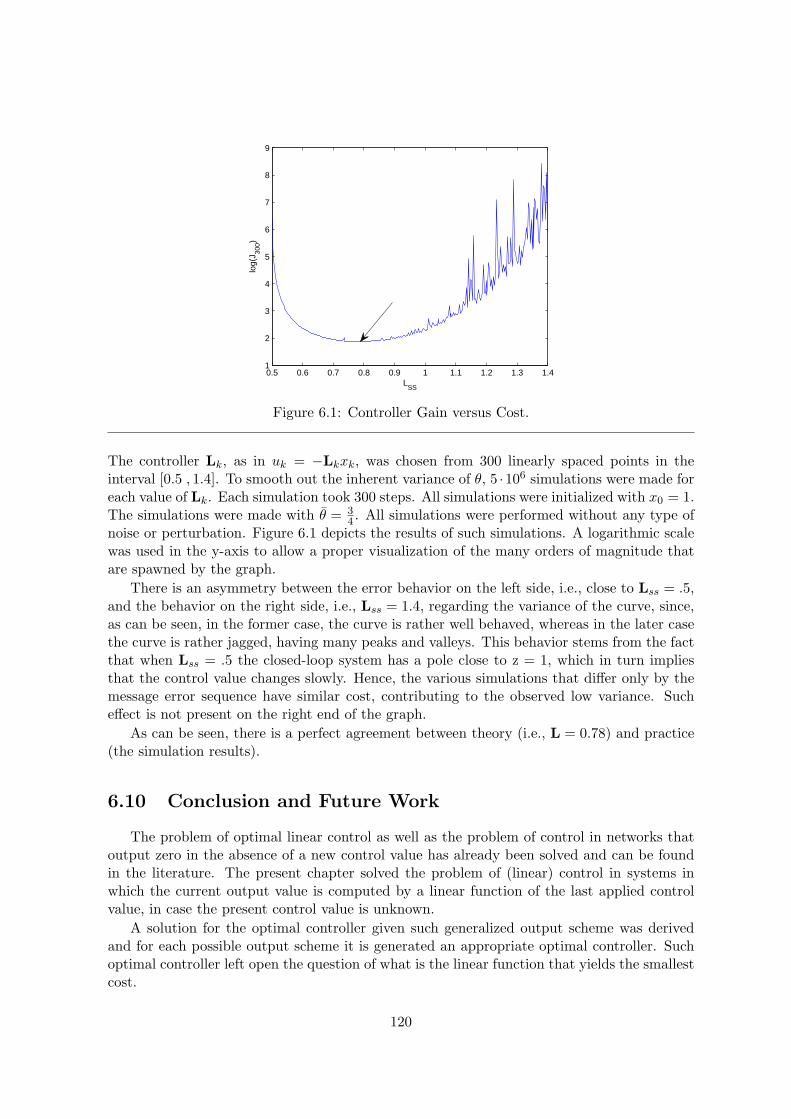
0.5 0.6 0.7 0.8 0.9 1 1.1 1.2 1.3 1.41

2

3

4

5

6

7

8

9

LSS

log(

J 300)

Figure 6.1: Controller Gain versus Cost.

The controller Lk, as in uk = −Lkxk, was chosen from 300 linearly spaced points in theinterval [0.5 , 1.4]. To smooth out the inherent variance of θ, 5 ·106 simulations were made foreach value of Lk. Each simulation took 300 steps. All simulations were initialized with x0 = 1.The simulations were made with θ = 3

4 . All simulations were performed without any type ofnoise or perturbation. Figure 6.1 depicts the results of such simulations. A logarithmic scalewas used in the y-axis to allow a proper visualization of the many orders of magnitude thatare spawned by the graph.

There is an asymmetry between the error behavior on the left side, i.e., close to Lss = .5,and the behavior on the right side, i.e., Lss = 1.4, regarding the variance of the curve, since,as can be seen, in the former case, the curve is rather well behaved, whereas in the later casethe curve is rather jagged, having many peaks and valleys. This behavior stems from the factthat when Lss = .5 the closed-loop system has a pole close to z = 1, which in turn impliesthat the control value changes slowly. Hence, the various simulations that differ only by themessage error sequence have similar cost, contributing to the observed low variance. Sucheffect is not present on the right end of the graph.

As can be seen, there is a perfect agreement between theory (i.e., L = 0.78) and practice(the simulation results).

6.10 Conclusion and Future Work

The problem of optimal linear control as well as the problem of control in networks thatoutput zero in the absence of a new control value has already been solved and can be foundin the literature. The present chapter solved the problem of (linear) control in systems inwhich the current output value is computed by a linear function of the last applied controlvalue, in case the present control value is unknown.

A solution for the optimal controller given such generalized output scheme was derivedand for each possible output scheme it is generated an appropriate optimal controller. Suchoptimal controller left open the question of what is the linear function that yields the smallestcost.

120

A necessary and sufficient condition for the optimality of the linear function was alsopresented. Moreover, a mechanism to compute such optimal controllers was devised. Suchcontroller was then compared with the controller of the architecture presented in earlierchapters.

Simulation results are in perfect agreement with the optimal control gain computed the-oretically.

121

Chapter 7

Oscillation Free Controller Change

7.1 Introduction and Motivation

The extraordinary development of microprocessors not only made ubiquitous the use ofcontrol networks on control systems as discussed in previous chapters, but it also made digitalcontrol the dominant control systems approach. When compared with conventional analogcontrollers, digital controllers of a given quality are usually less expensive, present higherflexibility and adaptability to different applications, are more scalable and can perform severalfunctions concurrently, not all necessarily related to control. Analog compensators, on theother hand, are usually developed in an application specific manner and can hardly be reusedfor other purposes.

Control systems are typically subject to strong, and often conflicting, constraints, forexample, relating to their jitter, message delivery, etc. On top of that, there is the factthat digital control processes are usually not the only task being executed by the respectiveprocessor, which often executes a multitude of tasks. As seen on Chapter 3, in order toguarantee that all tasks meet their requirements at each and every moment, these systems aredesigned according to their worst case requirements. However, designing systems accordingto the worst-case requirements of each task may lead to expensive and inefficient designs, fora myriad of reasons. For example, there are cases in which it is possible to guarantee that thetasks never enter in overload simultaneously, hence the requirements of such tasks is smallerthan the sum of the requirements of each individual task.

A number of approaches that make a more efficient use of system resources, in whichtask sets are not designed for the worst case requirements were put forward in the literature.Instead, each task runs at a given level. These level are set such that under normal condi-tions they lead to an underloaded system. Whenever a task requires more resources, it isgiven enough resources to successfully complete its current job, as discussed in Section 7.2.Obviously, this assumes that tasks will not simultaneously make a request for more resources.

In the specific case of control systems, many such approaches rely on controller changes,taking advantage of the monotonically increasing relationship between control performanceand resource utilization, as discussed on Sections 2.3.3 and 2.3.4 and references therein. Oneof the techniques that has been extensively investigated consists in using several controllers,designed to have different resource needs, and consequently, to exhibit different performancelevels. Therefore, less resource demanding, albeit less efficient, controllers are used wheneverthe system error is small, while more resource demanding and more efficient controllers are

123

selected when the system experiences a large error. The last comment was one example ofa situation that triggers a controller switch. Others examples include an overload situation(possibly caused by the switching of the remaining tasks) or because the controller is at themoment the plant that is being controlled has a different importance to the global system.

However, the contributions found in the literature have been essentially focused on therules for triggering the controller switching, like some of the approaches for resource opti-mization presented in Chapter 3, but neglected the full extent that such changes have in thesystem. That is, notwithstanding the aforementioned advantages of using controllers that cancommute, the controllers in question are designed for static operation.

In particular, switching controllers often causes output oscillations that may negate thepotential performance gains. More concretely, in the controller change methodologies hithertoproposed in the literature, controller transitions are almost always followed by an outputoscillation. At best, these oscillations degrade the quality of control. However, it may easilyhappen that such oscillations in turn cause another controller change, which itself triggers yetanother oscillation and so on and so forth. One example of this effect is provided in Section6.9. Consequently, systems with multiple controllers tend to oscillate between two or morecontrollers, even when the system conditions would otherwise be stationary, thus degradingthe quality of the control and wasting resources.

In this chapter, firstly, the cause of oscillations in the presence of period changes is pre-sented. Then, it is presented a solution, based in a change of basis matrix. An evaluationsection is also presented and it shows that important performance gains are achieved in keycontrol performance indicators such as overshoot, settling time and error.

This chapter intends to provide control system designers with the necessary theoreticaltools to predict and avoid oscillations that occur in systems that employ controller changes.

7.2 Related Work

The study of switching controllers began decades ago, hence it enjoys a vast body ofliterature. However, the study of oscillation free transitions remained a fringe topic betweenboth the control and scheduling communities. This fact rendered its associated literature notso vast. This section provides an overview of the scientific contributions that are both closeand relevant to the work presented in this chapter.

In [APM05] it is discussed the use of several controllers, each tuned to a given period. Intheir approach, the scheduler then chooses a controller of a given period according to the errorlevel. This idea was somehow complemented in [CVMC10], with a study of optimal transitionerror levels for each controller, though the former study was centered around distributedsystems whereas the latter was focused on centrally scheduled systems. Further work in thisarea includes the investigation of when a number of pre-calculated controllers outperformdynamically chosen ones, in terms of computational load, allowed periods, response time andrelated metrics.

Several studies, for example [CMVC06] and more prominently [AT09], discussed whetherthe controller changes should be based in instantaneous or in filtered/accumulated measuresof error. Other studies, such as [CMVC06], favor instantaneous measures, based in a numberof experiments that show that the advantages of filtering do not compensate the additionalcomputational burden. In [AT09] it is presented a similar experiment, although with differentsystems, and concludes that filtering was worthwhile. This apparent contradiction certainly

124

deserves a deeper study, which, however, it is out of the scope of this Thesis.In [CE00] and more recently in [CEBA02] the authors present a rather different approach.

Co-design is (re)introduced with a new set of goals and paradigms. Each controlled processhas a given weight and the goal of the scheduler is to assign the periods in a way that minimizesthe sum of the weights times the squared errors. More formally, let f(τj) =

∑k∈τj wke

2k be the

total error, given that it was chosen the schedule τj , i.e., the j possible parameter attributionof the task set and under such parameter assignment, the kth process has error ek and weightwk. Then the chosen schedule is:

τ = argmin (f(τj)) . (7.1)

However, in [BVM07] it is proposed to minimize a slightly different quantity which the au-thors call the quality of control. Nevertheless, the mechanism is somewhat similar to itspredecessors, hence it may produce similar parameter assignment to the tasks of the task set,and it may also present itself to be more difficult to minimize.

Using the CAN protocol, [AT09] discusses the advantages of period switching at thenetwork level, thus approaching a co-design perspective. In [LMVF08b] and references therein,a discussion regarding feedback scheduling is presented. Feedback scheduling can be looselydefined as a scheduling methodology in which the task’s current characteristics (e.g., period,worst-case execution time) are defined based on current operating conditions.

The problem of scheduling such processes has also made significant advances, one of themost relevant ones being the elastic task model [BLCA02]. Drawing from an analogy ofstrained springs, in which the sum of the displacements is equal to the total displacementand the displacement of each string is inversely proportional to its elastic coefficient, in thismethod the task’s utilization may be adjusted to have a given utilization level. Each task hasan individual weight that controls its relative level of adaptivity. This model is general enoughto be ported to the control scenario without major modifications. Nonetheless, it was furthergeneralized in [CHL06] for encompassing other types of minimization. It must be pointed outthat in all such studies it is assumed that there is a mechanism for correctly/optimally choosethe task’s weights. However, to the best of our knowledge, there are no studies addressingthis issue.

In [VMF+10] non-periodic controllers are presented. The controllers are executed andthen, based on the current state and error, the next activation instant is selected, i.e., it isself-triggered. However, this method has a few drawbacks and limitations. One of the mostimportant ones is that it implies a centralized architecture, since the controller must have anew sample at a moment that, in a distributed system, is not available. Additionally, eventhough a number of simulations were presented, it is not clear that there is no periodic con-troller that achieves the same quality of control. Furthermore, its erratic activation pattern,which was further discussed in [MVB09], renders its associated schedulers far more complex.

7.3 Controller Adaptation through Period Switch

7.3.1 Types of Controller Change

In general, controller changes are performed whenever the current controller, accordingto some criteria, is not the most suitable one to deal with the current situation. Differentcontroller characteristics can be modified. To systematize the presentation, the type of con-troller adaptations are categorized into three non-simultaneously exclusive classes: period

125

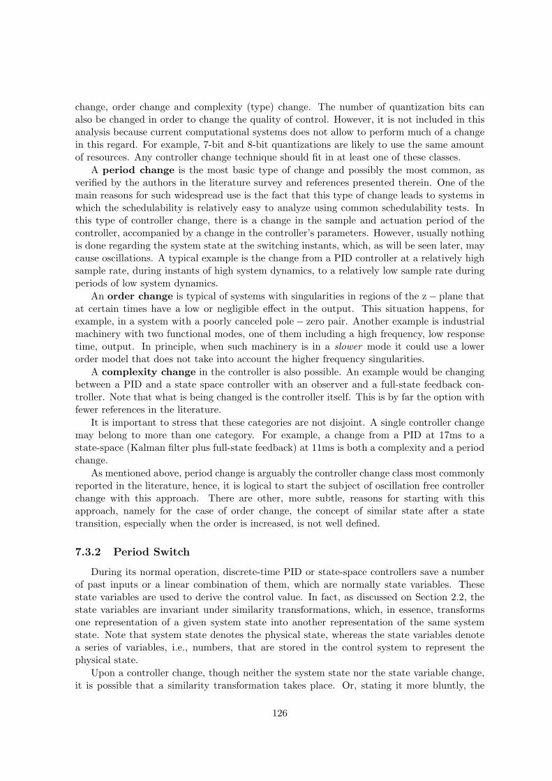
change, order change and complexity (type) change. The number of quantization bits canalso be changed in order to change the quality of control. However, it is not included in thisanalysis because current computational systems does not allow to perform much of a changein this regard. For example, 7-bit and 8-bit quantizations are likely to use the same amountof resources. Any controller change technique should fit in at least one of these classes.

A period change is the most basic type of change and possibly the most common, asverified by the authors in the literature survey and references presented therein. One of themain reasons for such widespread use is the fact that this type of change leads to systems inwhich the schedulability is relatively easy to analyze using common schedulability tests. Inthis type of controller change, there is a change in the sample and actuation period of thecontroller, accompanied by a change in the controller’s parameters. However, usually nothingis done regarding the system state at the switching instants, which, as will be seen later, maycause oscillations. A typical example is the change from a PID controller at a relatively highsample rate, during instants of high system dynamics, to a relatively low sample rate duringperiods of low system dynamics.

An order change is typical of systems with singularities in regions of the z− plane thatat certain times have a low or negligible effect in the output. This situation happens, forexample, in a system with a poorly canceled pole− zero pair. Another example is industrialmachinery with two functional modes, one of them including a high frequency, low responsetime, output. In principle, when such machinery is in a slower mode it could use a lowerorder model that does not take into account the higher frequency singularities.

A complexity change in the controller is also possible. An example would be changingbetween a PID and a state space controller with an observer and a full-state feedback con-troller. Note that what is being changed is the controller itself. This is by far the option withfewer references in the literature.

It is important to stress that these categories are not disjoint. A single controller changemay belong to more than one category. For example, a change from a PID at 17ms to astate-space (Kalman filter plus full-state feedback) at 11ms is both a complexity and a periodchange.

As mentioned above, period change is arguably the controller change class most commonlyreported in the literature, hence, it is logical to start the subject of oscillation free controllerchange with this approach. There are other, more subtle, reasons for starting with thisapproach, namely for the case of order change, the concept of similar state after a statetransition, especially when the order is increased, is not well defined.

7.3.2 Period Switch

During its normal operation, discrete-time PID or state-space controllers save a numberof past inputs or a linear combination of them, which are normally state variables. Thesestate variables are used to derive the control value. In fact, as discussed on Section 2.2, thestate variables are invariant under similarity transformations, which, in essence, transformsone representation of a given system state into another representation of the same systemstate. Note that system state denotes the physical state, whereas the state variables denotea series of variables, i.e., numbers, that are stored in the control system to represent thephysical state.

Upon a controller change, though neither the system state nor the state variable change,it is possible that a similarity transformation takes place. Or, stating it more bluntly, the

126

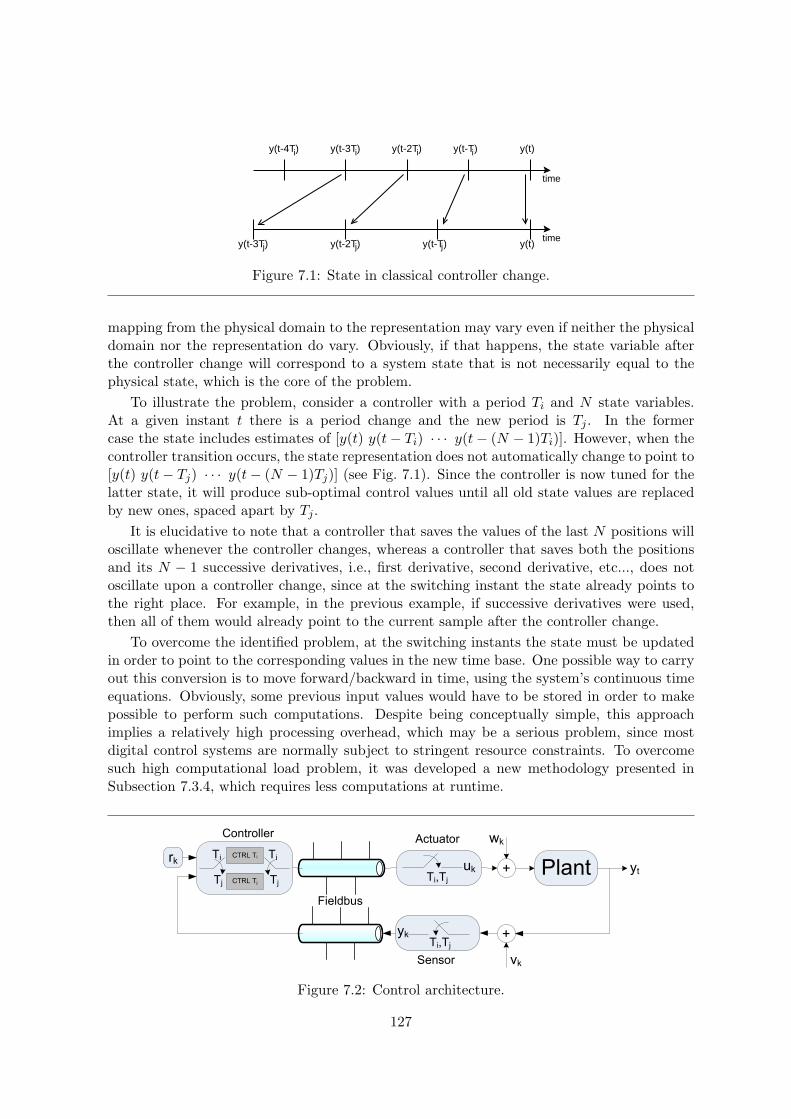
y(t)y(t-3T) y(t-2T)y(t-4T)

y(t-2T) y(t-T) y(t)y(t-3T)

y(t-T)

j

i ii i

jj

time

time

Figure 7.1: State in classical controller change.

mapping from the physical domain to the representation may vary even if neither the physicaldomain nor the representation do vary. Obviously, if that happens, the state variable afterthe controller change will correspond to a system state that is not necessarily equal to thephysical state, which is the core of the problem.

To illustrate the problem, consider a controller with a period Ti and N state variables.At a given instant t there is a period change and the new period is Tj . In the formercase the state includes estimates of [y(t) y(t− Ti) · · · y(t− (N − 1)Ti)]. However, when thecontroller transition occurs, the state representation does not automatically change to point to[y(t) y(t− Tj) · · · y(t− (N − 1)Tj)] (see Fig. 7.1). Since the controller is now tuned for thelatter state, it will produce sub-optimal control values until all old state values are replacedby new ones, spaced apart by Tj .

It is elucidative to note that a controller that saves the values of the last N positions willoscillate whenever the controller changes, whereas a controller that saves both the positionsand its N − 1 successive derivatives, i.e., first derivative, second derivative, etc..., does notoscillate upon a controller change, since at the switching instant the state already points tothe right place. For example, in the previous example, if successive derivatives were used,then all of them would already point to the current sample after the controller change.

To overcome the identified problem, at the switching instants the state must be updatedin order to point to the corresponding values in the new time base. One possible way to carryout this conversion is to move forward/backward in time, using the system’s continuous timeequations. Obviously, some previous input values would have to be stored in order to makepossible to perform such computations. Despite being conceptually simple, this approachimplies a relatively high processing overhead, which may be a serious problem, since mostdigital control systems are normally subject to stringent resource constraints. To overcomesuch high computational load problem, it was developed a new methodology presented inSubsection 7.3.4, which requires less computations at runtime.

Plantrk

Ti,Tjyk

wk

vk

yt

CTRL Ti

CTRL TjTi,Tj

ukTj

Ti Ti

Tj+

+

Controller

Fieldbus

Actuator

Sensor

Figure 7.2: Control architecture.

127

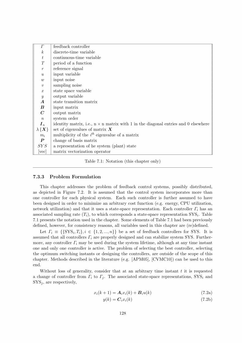
Γ feedback controllerk discrete-time variablet continuous-time variableT period of a functionr reference signalu input variablew input noisev sampling noisex state space variabley output variableA state transition matrixB input matrixC output matrixn system orderIn identity matrix, i.e., n× n matrix with 1 in the diagonal entries and 0 elsewhere

λ X set of eigenvalues of matrix Xmi multiplicity of the ith eigenvalue of a matrixP change of basis matrix

SY S a representation of he system (plant) state[vec] matrix vectorization operator

Table 7.1: Notation (this chapter only)

7.3.3 Problem Formulation

This chapter addresses the problem of feedback control systems, possibly distributed,as depicted in Figure 7.2. It is assumed that the control system incorporates more thanone controller for each physical system. Each such controller is further assumed to havebeen designed in order to minimize an arbitrary cost function (e.g. energy, CPU utilization,network utilization) and that it uses a state-space representation. Each controller Γi has anassociated sampling rate (Ti), to which corresponds a state-space representation SYSi. Table7.1 presents the notation used in the chapter. Some elements of Table 7.1 had been previouslydefined, however, for consistency reasons, all variables used in this chapter are (re)defined.

Let Γi ≡ SYSi, Ti, i ∈ 1, 2, ..., n be a set of feedback controllers for SYS. It isassumed that all controllers Γi are properly designed and can stabilize system SYS. Further-more, any controller Γi may be used during the system lifetime, although at any time instantone and only one controller is active. The problem of selecting the best controller, selectingthe optimum switching instants or designing the controllers, are outside of the scope of thischapter. Methods described in the literature (e.g. [APM05], [CVMC10]) can be used to thisend.

Without loss of generality, consider that at an arbitrary time instant t it is requesteda change of controller from Γi to Γj . The associated state-space representations, SYSi andSYSj , are respectively,

xi(k + 1) = Aixi(k) +Biu(k) (7.2a)

y(k) = Cixi(k) (7.2b)

128

and

xj(k + 1) = Ajxj(k) +Bju(k) (7.3a)

y(k) = Cjxj(k) (7.3b)

The problem thus consists in devising a mechanism to switch from SYSi to SYSj withoutoscillation, i.e., finding the value xj in the space of SYSj that corresponds to the state xi inSYSi at any arbitrary time.

As an additional requirement, the online part of such mechanism must be lightweight,both in terms of processing and memory, since the state conversions must be performedduring runtime, upon controller changes, in resource-constrained hardware.

7.3.4 Proposed Solution

The solution that is proposed in this chapter consists, firstly, in defining an auxiliary rep-resentation. The application of the similarity transformation of such auxiliary representation,first on the transition matrix and then on the input/output matrix, leads to a Sylvester andto a simpler linear equation, respectively. The resulting Sylvester equation is homogeneous,thus classic solving methods are inadequate, leading to the use of the Kronecker product.From this process it is extracted an ensemble of matrices that verify the transition matrixcondition. Furthermore, any non-singular linear combination of such matrices is also a solu-tion. Finally, it is searched for a linear combination of the matrix ensemble that also verifiesthe input/output matrix similarity equation. The remaining of this section presents, in detail,each one of these steps.

To carry out the state conversion, first, consider an auxiliary representation SYSja, whichis sampled at rate Tj but its continuous time version has a state equal to the state of SYSi.Such representation can be found, for instance, by discretizing the continuous-time version ofSYSi with period Tj . By construction, SYSja can be written as

xja(k + 1) = Ajaxja(k) +Bjau(k) (7.4a)

y(k) = Cixja(k) (7.4b)

The introduction of SYSja turns the original problem into a simpler one, i.e., a change ofbasis problem. Since, by design, xi = xja and both SYSja and SYSj are sampled at the samerate, there should be a matrix P such that xj = P xja. The existence and uniqueness of suchmatrix is a standard result [dM10].

To find P , it can be used the Sylvester equation 1: Aja = P−1AjP , or

PAja −AjP = 0 (7.5)

However, classical efficient approaches, e.g. [BS72, GNVL79], fail to give satisfactorysolutions to this particular problem, since they always return the trivial solution, i.e., P = 0.It is noteworthy that this equation also appears in robust pole placement techniques, asattested by [Var00] and references therein. In fact, this mechanism is so widespread that it iseven used in standard commercial products such as the Matlab R⃝ function place. However,the mechanisms used to solve it in that context are not easily portable to this problem.

1AX +XB = C in which A = −Aj , B = Aja and C = 0.

129

Therefore, it was opted to use the Kronecker product approach. In this approach, Equation(7.5) is transformed into: (

ATja ⊗ In − In ⊗Aj

)vec(P ) = 0 (7.6)

where vec(P ) is a vectorized version of the matrix P and In is the (n× n) identity matrix.The vectorization operation as described by the vec(X), is a matrix operation that stacks

column wise, i.e., in order of the column number, the columns of matrix X into a singlecolumn, i.e.

vec([x1 x2 · · · xn−1 xn]) =[x′1 x

′2 · · · x′n−1 x

′n

]′(7.7)

in which xi is the ith column of X.Equation (7.6) is an eigen problem, associated with the eigenvalue 0. Eigen problems are

the problems of finding the vectors that when applied to a given function, return an amplified(by a factor equal to the corresponding eigenvalue) version of the vector in question.

The solution of the eigen problem induced by Equation (7.6) is a series of vectors that,when passed back into the initial matrix space (the inverse of vec), gives rise to a series of eigenmatrices to which any non-singular linear combination is also a solution of Equation (7.5).This stems from a known result of linear algebra, which states that any linear combinationof eigenvectors associated with the same eigenvalue is also an eigenvector associated with theeigenvalue in question.

This principle is combined to the fact that any eigenvector associated with the eigen-value 0 is a solution of Equation (7.5), implying that any linear combination of a solution ofEquation (7.6) is also a solution of Equation (7.5).

Regarding the dimensionality of the space of eigen matrices that are solutions of Equa-tion (7.6), naıvely it could be said that Equation (7.6) in general does not have any eigenmatrix associated with the eigenvalue 0. However, it is well known that the eigenvalues of(A⊗ In − In ⊗B) (with A,B square matrices of size n) are λi(A)−λj(B), where λi(X) isthe ith eigenvalue of matrix X. In this particular case, A and B have the same eigenvaluesdue to the fact that they are each other’s transposes, hence each eigenvalue of A producesm2

i zero eigenvalues in the matrix P , where mi is the multiplicity of the ith eigenvalue. Thus,P has an eigenvalue of 0 with multiplicity

∑qi=1m

2i ≥ n, where q is the number of distinct

eigenvalues of A.Due to the similarity transformation, matrix P must verify (note that there was no par-

ticular reason to apply the similarity transformation to the input matrices, i.e., it could aswell be applied to the output matrices)

PBja = Bj . (7.8)

Equations (7.5) (or (7.6)) and (7.8) define matrix P , though, as is discussed below, theymay not define a single matrix. More precisely, the first equation defines a rank three (3-dimensional) tensor, that is conveniently written as a number of eigen matrices, as pointedout above, and the product of such matrix by matrix Bja can be written as:

PBja =

(∑i

ωiP i

)Bja, (7.9)

where P i are the eigen matrices as computed from Equation (7.6) and ωi are unknowncoefficients. Determining the unknown coefficients would implicitly solve the problem. The

130

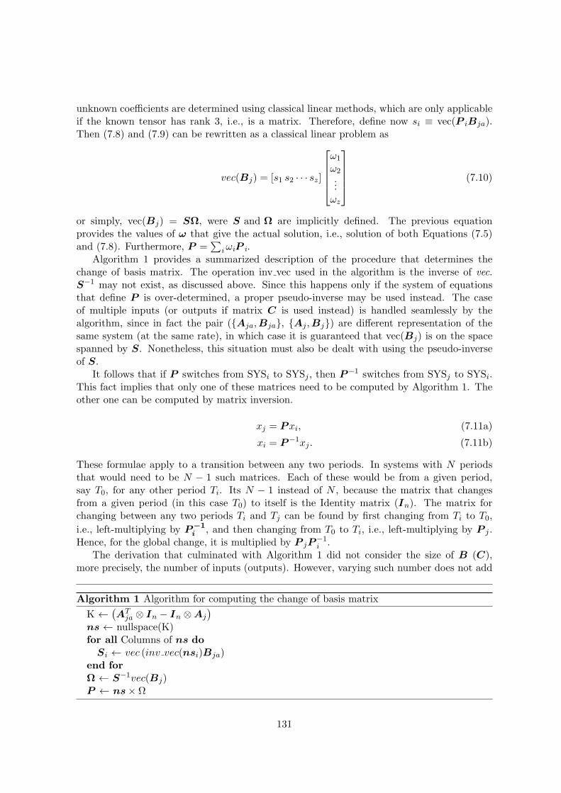
unknown coefficients are determined using classical linear methods, which are only applicableif the known tensor has rank 3, i.e., is a matrix. Therefore, define now si ≡ vec(P iBja).Then (7.8) and (7.9) can be rewritten as a classical linear problem as

vec(Bj) = [s1 s2 · · · sz]

ω1

ω2...ωz

(7.10)

or simply, vec(Bj) = SΩ, were S and Ω are implicitly defined. The previous equationprovides the values of ω that give the actual solution, i.e., solution of both Equations (7.5)and (7.8). Furthermore, P =

∑i ωiP i.

Algorithm 1 provides a summarized description of the procedure that determines thechange of basis matrix. The operation inv vec used in the algorithm is the inverse of vec.S−1 may not exist, as discussed above. Since this happens only if the system of equationsthat define P is over-determined, a proper pseudo-inverse may be used instead. The caseof multiple inputs (or outputs if matrix C is used instead) is handled seamlessly by thealgorithm, since in fact the pair (Aja,Bja, Aj ,Bj) are different representation of thesame system (at the same rate), in which case it is guaranteed that vec(Bj) is on the spacespanned by S. Nonetheless, this situation must also be dealt with using the pseudo-inverseof S.

It follows that if P switches from SYSi to SYSj , then P−1 switches from SYSj to SYSi.This fact implies that only one of these matrices need to be computed by Algorithm 1. Theother one can be computed by matrix inversion.

xj = Pxi, (7.11a)

xi = P−1xj . (7.11b)

These formulae apply to a transition between any two periods. In systems with N periodsthat would need to be N − 1 such matrices. Each of these would be from a given period,say T0, for any other period Ti. Its N − 1 instead of N , because the matrix that changesfrom a given period (in this case T0) to itself is the Identity matrix (In). The matrix forchanging between any two periods Ti and Tj can be found by first changing from Ti to T0,

i.e., left-multiplying by P−1i , and then changing from T0 to Ti, i.e., left-multiplying by P j .

Hence, for the global change, it is multiplied by P jP−1i .

The derivation that culminated with Algorithm 1 did not consider the size of B (C),more precisely, the number of inputs (outputs). However, varying such number does not add

Algorithm 1 Algorithm for computing the change of basis matrix

K ←(AT

ja ⊗ In − In ⊗Aj

)ns ← nullspace(K)for all Columns of ns do

Si ← vec (inv vec(nsi)Bja)end forΩ ← S−1vec(Bj)P ← ns× Ω

131

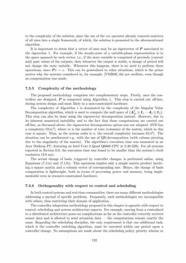
to the complexity of the solution, since the use of the vec operator already converts matricesof all sizes into a single framework, of which, the solution is presented in the aforementionedalgorithm.

It is important to stress that a vector of ones may be an eigenvector of P associated tothe eigenvalue 1. For example, if the steady-state of a variable-phase representation is inthe space spanned by such vector, i.e., if the state variable is comprised of precisely (currentand) past values of the outputs, then whenever the output is stable, a change of period willnot change the state variable. Whenever this happens, there is no need to perform theseoperations, since Px = x. This can be generalized to other situations, which is the primemotive why the systems considered in, for example, [VMB08] did not oscillate, even thoughno compensation was made.

7.3.5 Complexity of the methodology

The proposed methodology comprises two complementary steps. Firstly, once the con-trollers are designed, P is computed using Algorithm 1. This step is carried out off-line,during system design and most likely in a non-constrained hardware.

The complexity of Algorithm 1 is dominated by the complexity of the Singular ValueDecomposition algorithm, which is used to compute the null space of

(AT

ja ⊗ In −Aj ⊗ In

).

This step can also be done using the eigenvector decomposition instead. However, due toits inherent numerical instability and to the fact that these computations are carried outoff-line, as discussed above, the eigenvector decomposition option was not adopted. SVD hasa complexity O(m3), where m is the number of rows (columns) of the matrix, which in thiscase is square. Thus, as the system order is n, the overall complexity becomes O(n6). Thesituation can be ameliorated e.g. with the use of QR-decomposition (with column pivotingdue to the singularity of the matrix). The algorithm’s execution time was measured in anAcer Desktop PC, featuring an Intel Core 2 Quad Q6600 CPU at 2.40 GHz. For all systemsreported in Section 6.9, the execution time was found to be smaller than the system’s clockresolution (3.9 ms).

The actual change of basis, triggered by controller changes, is performed online, usingEquations (7.11a) and (7.11b). This operation implies only a simple matrix product involv-ing a square matrix and a column vector of corresponding size. Hence, the change of basiscomputation is lightweight, both in terms of processing power and memory, being imple-mentable even in resource-constrained hardware.

7.3.6 Orthogonality with respect to control and scheduling

In both control systems and real-time communities, there are many different methodologiesaddressing a myriad of specific problems. Frequently, such methodologies are incompatiblewith others, thus restricting their domain of application.

The controller adaptation methodology proposed in this chapter is agnostic with respect tocontrol, scheduling and system architecture aspects. For example, moving from a centralizedto a distributed architecture poses no complications as far as the controller correctly receivessensor data and is allowed to send actuation data — the computations remain exactly thesame. Regarding the scheduling discipline, the only requirement is that one additional task,which is the controller switching algorithm, must be executed within one period upon acontroller change. No assumptions are made about the scheduling policy, priority scheme or

132

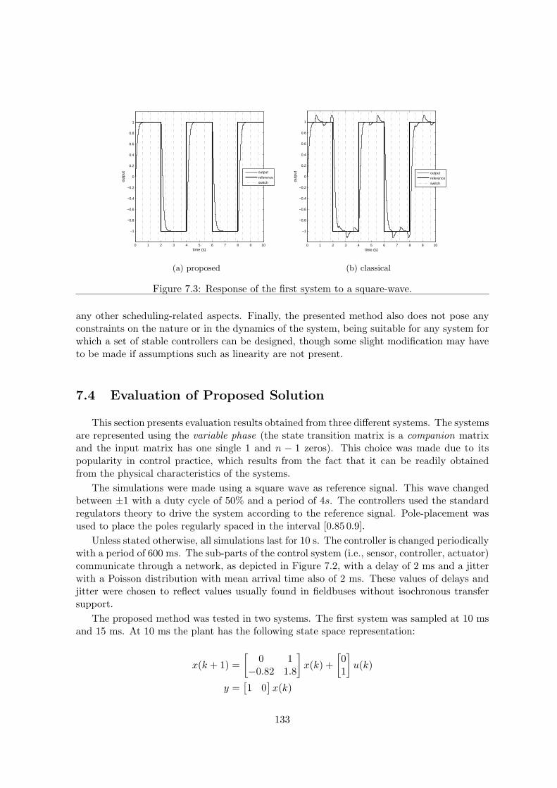
0 1 2 3 4 5 6 7 8 9 10

−1

−0.8

−0.6

−0.4

−0.2

0

0.2

0.4

0.6

0.8

1

time (s)

outp

ut

output

reference

switch

(a) proposed

0 1 2 3 4 5 6 7 8 9 10

−1

−0.8

−0.6

−0.4

−0.2

0

0.2

0.4

0.6

0.8

1

time (s)

outp

ut

output

reference

switch

(b) classical

Figure 7.3: Response of the first system to a square-wave.

any other scheduling-related aspects. Finally, the presented method also does not pose anyconstraints on the nature or in the dynamics of the system, being suitable for any system forwhich a set of stable controllers can be designed, though some slight modification may haveto be made if assumptions such as linearity are not present.

7.4 Evaluation of Proposed Solution

This section presents evaluation results obtained from three different systems. The systemsare represented using the variable phase (the state transition matrix is a companion matrixand the input matrix has one single 1 and n − 1 zeros). This choice was made due to itspopularity in control practice, which results from the fact that it can be readily obtainedfrom the physical characteristics of the systems.

The simulations were made using a square wave as reference signal. This wave changedbetween ±1 with a duty cycle of 50% and a period of 4s. The controllers used the standardregulators theory to drive the system according to the reference signal. Pole-placement wasused to place the poles regularly spaced in the interval [0.85 0.9].

Unless stated otherwise, all simulations last for 10 s. The controller is changed periodicallywith a period of 600 ms. The sub-parts of the control system (i.e., sensor, controller, actuator)communicate through a network, as depicted in Figure 7.2, with a delay of 2 ms and a jitterwith a Poisson distribution with mean arrival time also of 2 ms. These values of delays andjitter were chosen to reflect values usually found in fieldbuses without isochronous transfersupport.

The proposed method was tested in two systems. The first system was sampled at 10 msand 15 ms. At 10 ms the plant has the following state space representation:

x(k + 1) =

[0 1

−0.82 1.8

]x(k) +

[01

]u(k)

y =[1 0

]x(k)

133

0 1 2 3 4 5 6 7 8 9 10

−1

−0.5

0

0.5

1

time (s)

outp

ut

output

reference

switch

(a) proposed

0 1 2 3 4 5 6 7 8 9 10

−1

−0.5

0

0.5

1

time (s)

outp

ut

output

reference

switch

(b) classical

Figure 7.4: Response of second system to a square-wave

At 15 ms the plant’s state space equations are:

x(k + 1) =

[0 1

−0.6109 1.5694

]x(k) +

[01

]u(k)

y =[0.3009 1.7783

]x(k)

Figure 7.3 a) depicts the system behavior when the oscillation control technique proposedin this chapter is used, while Figure 7.3 b) depicts the results obtained in identical conditions,with the exception that the oscillation control technique is absent. By simple observation itcan be concluded that the proposed approach behaves as expected, exhibiting no oscillations,whereas in the classical approach controller switchings result in output oscillations.

The second system commutes between sampling periods 16 ms and 20 ms, with a plantthat has the following representations at each respective period:

x(k + 1) =

0 1.0000 00 0 1.0000

0.3150 −1.4300 2.1000

x(k) +

001

u(k)

y(k) =[0 1

]x(k)

and

x(k + 1) =

0 1.0000 00 0 1.0000

0.2360 −1.1990 1.9373

x(k) +

001

u(k)

y(k) =[−0.0172 0.3045 1.4277

]x(k)

Figure 7.4 shows the simulation results of this system. Once again, the classical approachcaused the system to oscillate, whereas with the approach proposed in this chapter the outputdoes not oscillate.

Several measurements were made to quantify the improvements shown in Figures 7.3 and7.4. They are summarized in Table 7.2. The first row of this table shows the rise-time of the

134

different systems. The proposed and the classical methods have rather similar values becauseduring the rise time window there were no controller transitions.

The second row of Table 7.2 shows the overshoot values. The proposed mechanism does notexhibit any overshoot because it does not oscillate despite the controller changes, a propertythat classical approaches lack. A similar situation is seen in the settling time, since classicalapproaches, under controller change, never reach a state that can be considered steady (5%error band).

ISE =

∫ T

0(y(t)− r(t))2 dt (7.12)

The ISE presented in the next to last row of Table 7.2 is computed according to Equation(7.12), in which T is the duration of the experiment, y(t) is the output signal and r(t) isthe reference signal. The improvement in the ISE does not seem to be substantive, mostlydue to the fact that the controllers are changed with a relatively low frequency. Hence, theISE is dominated by the time that the systems spend tracking the input signal. Note thatthe impact of controller-change induced oscillations is higher on the slower system, since theassociated recovery time is higher. This effect appears distinguishably when comparing theISE of the first (faster dynamics) and second (slower dynamics) systems. The faster systemexperiences an ISE reduction of 3.1%, while the slower system has an ISE reduction of 9.8%.

To highlight the controller change’s impact on the ISE, the corrected ISE was also com-puted, shown in the last row of Table 7.2. This modified ISE value is computed only for pointsin which both the reference and output signals are slowly varying, hence removing the impactof the reference signal changes, and thus the tracking error. With this metric the perfor-mance difference becomes much more evident. The corrected ISE is essentially null for bothsystems, when the oscillation control technique is applied. Note that the absolute value of thecorrected ISE is lower for system two because its output is stable during a shorter amount oftime, thereby reducing the time interval during which the corrected ISE is computed.

The final simulation presents an example of a system in which a controller change causesan oscillation, that in turn causes another controller change, so on and so forth. The systemchanges between a sample rate of 10 ms and 15 ms, according to the output error. There aretwo threshold values for the estimate of the output error, to induce hysteresis. The higherthreshold is set to 0.80 and the lower threshold is set to 0.10. The system remains at thehigher rate as long as the lower threshold is not crossed. Similarly, it remains at the lowersampling rate as long as the higher threshold is not crossed. At the highest sampler rate, i.e.,

SYS1 prop SYS1 classic SYS2 prop SYS2 classic

Rise time 247ms 256ms 525ms 585ms

Overshoot 0% 13.63% 0% 20.9%

Settling time (5%) 439ms undefined 887ms undefined

ISE 1584 1633 4051 4448

corrected ISE 1.74× 10−6 14.19 2.93× 10−6 3.59

Table 7.2: Metrics comparison

135

0 0.5 1 1.5 2

0

0.2

0.4

0.6

0.8

1

1.2

1.4

1.6

1.8

2

time (s)

outp

ut

output

reference

(a) proposed

0 0.2 0.4 0.6 0.8 1 1.2 1.4 1.6 1.8 2

0

0.2

0.4

0.6

0.8

1

1.2

1.4

1.6

1.8

2

time (s)

outp

ut

output

reference

(b) classical

Figure 7.5: Example of system locked in oscillations

10ms, the system is represented by:

x(k + 1) =

[0 1

−0.6400 1.5217

]x(k) +

[01

]u(k)

y =[1 0

]x(k)

At the sampling rate of 15 ms it has the representation:

x(k + 1) =

[0 1

−0.5120 1.2751

]x(k) +

[01

]u(k)

y =[1.5950 0.4073

]x(k)

Figure 7.5 depicts the behavior of such system. The continuous controller switchingpattern is evident. It is also evident that the presented approach completely avoids it.

7.5 Conclusion

Dynamically switching controllers in order to always have active the controller that usesthe lowest possible amount of resources, while guaranteing a minimum quality of control, hasbeen a field of intense research. However, in existing approaches controller changes are oftenfollowed by output oscillations, which may degrade the quality of control and waste resources.

This chapter investigated the origin of such output oscillations, which are, in essence, dueto the state variables not being in agreement before and after the controller switchings. Tosolve this problem, a novel mechanism, which finds a change of basis matrix that turns astate variable under a given representation into another one, was developed. During runtime,this mechanism only requires a simple matrix product, thus being implementable even inresource-constrained hardware, as those typically found in control system applications.

Simulations of diverse distributed systems, subject to network contention, were carriedout. The obtained results are in perfect accordance with the expectations. The same systems,subject to the same stimulus, experienced oscillations when the classical approaches wereemployed, while such oscillations did not occur when the adaptation method presented in thischapter was used. Quantitatively, the absence of such oscillations results in the nullificationof the overshoot and ISE due to controller changes.

136

Chapter 8

Toward DeterministicImplementations of (m,k)–firmSchedulers

8.1 Introduction

From encoded video files that can withstand the loss of certain packets to control mes-sages that can be dropped without a serious deterioration of the quality-of-control to controlapplications that can loose some messages without a significant deterioration of the qualityof control, it is somewhat common to have tasks that tolerate a number of packet misses, theso called (m, k)–firm tasks.

In recent years, a number of advances were made concerning the implementation of sched-ulers capable of handling this type of tasks. However, most of the hitherto implementedschedulers are of the so called probabilistic (m, k)–firm type, which means that though thescheduler may try to reduce the amount of time in which the (m, k)–firm guarantees are notmet, the primary goal is to ensure that on average m out of k job executions are met. Suchapproach may have deleterious effects on the scheduled tasks. For example, in the videocase above, the decoder may not be capable of correctly decode certain frames if some otherparticular frames are missing.

The other type of (m, k)–firm schedulers is called deterministic and it ensures that forany group of k consecutive jobs at least m are executed. Nevertheless, all deterministicschedulers that have been presented in the literature suffer from the same illness, namelythey are schedulable if they are also EDF-schedulable, a point that will be made more clearthroughout this chapter. This fact renders them of little use, since one could simply use EDFinstead and execute all jobs from such tasks.

This chapter presents a new scheduler that can schedule tasks with utilizations that wouldotherwise be greater than one, a feat that, as will be seen, cannot be achieved by any other(m, k)–firm scheduler. Such task sets are scheduled by dropping jobs that do not substantiallycontribute to the overall quality of the system.

Both a static and a dynamic scheduler will be presented. The scheduler is dynamic, in thesense that whether a given job is executed does not depend only on the priority with which itsassociated task generates it, i.e., the priorities are associated to jobs as opposed to tasks. Theguiding lines for the construction of such schedulers are presented. It is shown that this new

137

approach can schedule task sets with higher utilizations. In particular, all task sets schedulableby classical static schedulers are also schedulable by the dynamic scheduler presented herein,however the converse is not true. Furthermore, when the task set is schedulable both staticallyand dynamically, in general the dynamic scheduler achieves utilizations greater than the staticone. In this chapter, in addition to the dynamical scheduler, a novel static scheduler ispresented, which is derived from the dynamic scheduler, that similarly can schedule task setswith utilizations, that if all tasks were set to (k, k)–firm would be greater than one.

8.1.1 On the Use of (m,k)-firm Schedulers for Control Purposes

As discussed in Section 3.4 and in references therein, in control applications it is possibleto significantly reduce the number of jobs that are executed, i.e., the number of controlvalues that are computed/delivered, while incurring only a small increase of the cost function.Evidently, this reduction of the number of computed control values must be accompanied bya change of the control law.

Deterministic (m, k)–firm schedulers are best suited for used in control applications, be-cause probabilistic schedulers do not preclude the possibility of long periods without anyexecution. Such long periods without service could bring about some catastrophic outcomesto the controlled system.

Hence, the obvious choice of (m, k)–firm schedulers for use in control systems are thedeterministic ones. In fact, most of the existing strategies, as seen in Section 3.4, use arepeating pattern of executions and non executions. However, as will be shown in this chapter,the use of these repeating patterns may jeopardize their own schedulability.

For this reason, it is proposed in this chapter, a dynamic (m, k)–firm scheduler that canbe used in control settings. Note that the efficient use of network resources in control settingsis the main drive for the use of this type of schedulers. Notwithstanding this observations,the proposed scheduler can be used for the scheduling of CPU tasks without any modificationwhatsoever.

This scheduler can be used, for instance, in the implementation of the networked controlarchitecture presented in Chapter 4.

8.2 Static (Circular) (m,k)-firm Schedulers

This section generalizes some theorems in the literature. The first theorem generalizes thetheorem proved in [Ram99] that states that upper mechanical (m, k)–firm frames generate(m, k)–firm sequences that always meet the respective guarantees. The theorem is generalizedfor any frame with the respective size and number of mandatory jobs. The second theoremhelps to understand the periodic nature of (m, k)–firm sequences. In [QH00] is proven thatthe use of the Chinese reminder algorithm can be used to schedule (m, k)–firm task sets. Thetheorem is generalized to allow any algorithm that handles periodically repeating activationpatterns. This is of uttermost importance because the Chinese reminder algorithm is knownto be NP-hard, i.e., it cannot be solved in polynomial time.

These theorems will in turn be fundamental at establishing the improvements of thedynamical scheduler proposed in this chapter. But before that, a number of basic definitionsare in order.

138

Definition. An (m, k)–firm frame is any group of k bits in which m and only m bits areones.

Definition. A job is optional if the rightmost bit of the (m, k)–firm frame associated with itstask is zero, otherwise the job is mandatory.

Definition. An (m, k)–firm sequence is any sequence of job executions in which for any groupof k consecutive job activations, at least m are executed.

Furthermore, in this analysis it is made a number of assumptions:

• An optional job is executed if and only if its execution does not cause the miss of adeadline of a mandatory job.

• An optional job is executed if and only if it will be able to complete its execution withinits respective deadline.

• Whenever a job is released, regardless of being executed or not, unless some patternbreaking event occurs, the whole (m, k)–firm frame associated with it is rotated one bitto the left.

• Tasks release jobs periodically, regardless of the job’s priority.

The next theorem helps to understand the name (m, k)–firm frame

Theorem 1. Any (m, k)–firm frame generates an (m, k)–firm sequence.

Proof. The job execution sequence is encoded into the (m, k)–firm frame. So, if the sequenceis rotated one bit to the left, then the bit sequence will be exactly the job execution sequence,where the newer job corresponds to the rightmost and the older one to the second from theright. Hence, in the worst case, when only mandatory jobs get executed, there will be exactlym jobs executed out of k, corresponding to the number of ones in the frame.

This theorem removes the distinctiveness of any special sequence, such as the upper me-chanical word used in [Ram99] and an intuition of it was the basis of the work in [QH00].

The next theorem helps to understand the static nature of (m, k)–firm frame.

Theorem 2. k is a period of any task whose job sequence is generated by an (m, k)–firmframe. Or restating, the jobs activated at time ti and at time ti + k ∗ T , with T the period ofthe job in question, are either both mandatory or both optional.

Proof. Given the way in which jobs are set as mandatory or optional, to prove the theorem,it suffices to prove the periodicity of the (m, k)–firm sequence. Now, since each job activationtriggers one rotation of the (m, k)–firm frame, then k activations will trigger k rotations ofthe (m, k)–firm frame. Since the (m, k)–firm frame is k bits long, k rotations put it back inits original state.

Note, however, that k is not necessarily the smallest period, since the (m, k)–firm framemay have an internal period. Notwithstanding, if the frame does have an internal period, letn be the number of periods within the frame, then it is easy to prove that a (mn ,

kn)–firm frame

built with the last (or any consecutive) kn bits of the initial frame generates a job sequence

with mandatory/optional jobs at the same places. Moreover, this new frame sequence has a

139

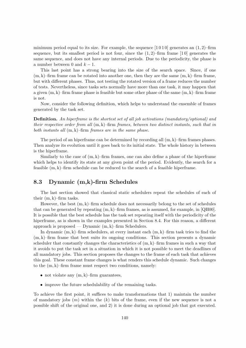
minimum period equal to its size. For example, the sequence [1 0 1 0] generates an (1, 2)–firmsequence, but its smallest period is not four, since the (1, 2)–firm frame [1 0] generates thesame sequence, and does not have any internal periods. Due to the periodicity, the phase isa number between 0 and k − 1.

This last point has a strong bearing into the size of the search space. Since, if one(m, k)–firm frame can be rotated into another one, then they are the same (m, k)–firm frame,but with different phases. Thus, not testing the rotated version of a frame reduces the numberof tests. Nevertheless, since tasks sets normally have more than one task, it may happen thata given (m, k)–firm frame phase is feasible but some other phase of the same (m, k)–firm frameis not.

Now, consider the following definition, which helps to understand the ensemble of framesgenerated by the task set.

Definition. An hiperframe is the shortest set of all job activations (mandatory/optional) andtheir respective order from all (m, k)–firm frames, between two distinct instants, such that inboth instants all (m, k)–firm frames are in the same phase.

The period of an hiperframe can be determined by recording all (m, k)–firm frames phases.Then analyze its evolution until it goes back to its initial state. The whole history in betweenis the hiperframe.

Similarly to the case of (m, k)–firm frames, one can also define a phase of the hiperframewhich helps to identify its state at any given point of the period. Evidently, the search for afeasible (m, k)–firm schedule can be reduced to the search of a feasible hiperframe.

8.3 Dynamic (m,k)-firm Schedules

The last section showed that classical static schedulers repeat the schedules of each oftheir (m, k)–firm tasks.

However, the best (m, k)–firm schedule does not necessarily belong to the set of schedulesthat can be generated by repeating (m, k)–firm frames, as is assumed, for example, in [QH00].It is possible that the best schedule has the task set repeating itself with the periodicity of thehiperframe, as is shown in the examples presented in Section 8.4. For this reason, a differentapproach is proposed — Dynamic (m, k)–firm Schedulers.

In dynamic (m, k)–firm schedulers, at every instant each (m, k)–firm task tries to find the(m, k)–firm frame that best suits its ongoing conditions. This section presents a dynamicscheduler that constantly changes the characteristics of (m, k)–firm frames in such a way thatit avoids to put the task set in a situation in which it is not possible to meet the deadlines ofall mandatory jobs. This section proposes the changes to the frame of each task that achievesthis goal. These constant frame changes is what renders this schedule dynamic. Such changesto the (m, k)–firm frame must respect two conditions, namely:

• not violate any (m, k)–firm guarantees,

• improve the future schedulability of the remaining tasks.

To achieve the first point, it suffices to make transformations that 1) maintain the numberof mandatory jobs (m) within the (k) bits of the frame, even if the new sequence is not apossible shift of the original one, and 2) it is done during an optional job that got executed.

140

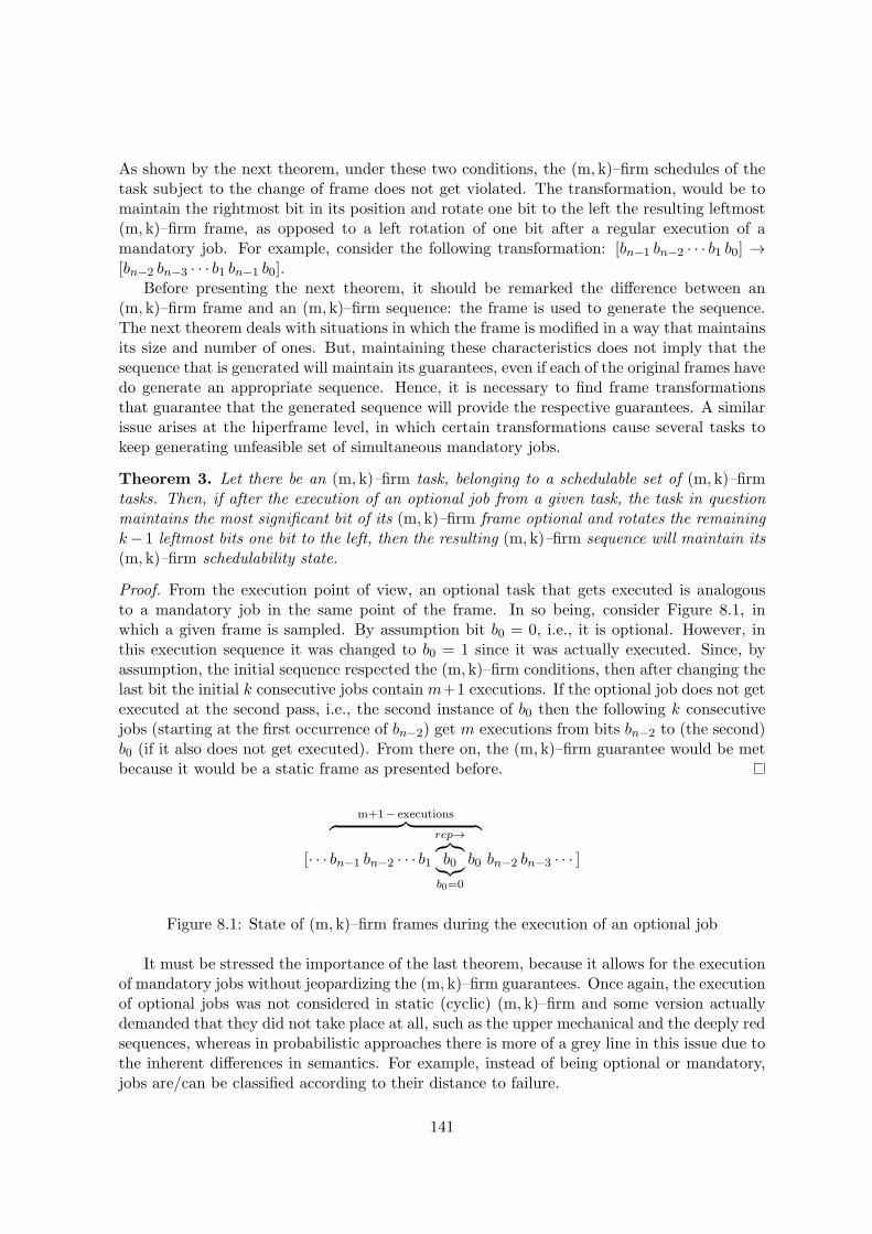
As shown by the next theorem, under these two conditions, the (m, k)–firm schedules of thetask subject to the change of frame does not get violated. The transformation, would be tomaintain the rightmost bit in its position and rotate one bit to the left the resulting leftmost(m, k)–firm frame, as opposed to a left rotation of one bit after a regular execution of amandatory job. For example, consider the following transformation: [bn−1 bn−2 · · · b1 b0] →[bn−2 bn−3 · · · b1 bn−1 b0].

Before presenting the next theorem, it should be remarked the difference between an(m, k)–firm frame and an (m, k)–firm sequence: the frame is used to generate the sequence.The next theorem deals with situations in which the frame is modified in a way that maintainsits size and number of ones. But, maintaining these characteristics does not imply that thesequence that is generated will maintain its guarantees, even if each of the original frames havedo generate an appropriate sequence. Hence, it is necessary to find frame transformationsthat guarantee that the generated sequence will provide the respective guarantees. A similarissue arises at the hiperframe level, in which certain transformations cause several tasks tokeep generating unfeasible set of simultaneous mandatory jobs.

Theorem 3. Let there be an (m, k)–firm task, belonging to a schedulable set of (m, k)–firmtasks. Then, if after the execution of an optional job from a given task, the task in questionmaintains the most significant bit of its (m, k)–firm frame optional and rotates the remainingk− 1 leftmost bits one bit to the left, then the resulting (m, k)–firm sequence will maintain its(m, k)–firm schedulability state.

Proof. From the execution point of view, an optional task that gets executed is analogousto a mandatory job in the same point of the frame. In so being, consider Figure 8.1, inwhich a given frame is sampled. By assumption bit b0 = 0, i.e., it is optional. However, inthis execution sequence it was changed to b0 = 1 since it was actually executed. Since, byassumption, the initial sequence respected the (m, k)–firm conditions, then after changing thelast bit the initial k consecutive jobs contain m+1 executions. If the optional job does not getexecuted at the second pass, i.e., the second instance of b0 then the following k consecutivejobs (starting at the first occurrence of bn−2) get m executions from bits bn−2 to (the second)b0 (if it also does not get executed). From there on, the (m, k)–firm guarantee would be metbecause it would be a static frame as presented before.

[· · ·

m+1− executions︷︸︸︷bn−1 bn−2 · · · b1

rep→︷︸︸︷b0︸︷︷︸

b0=0

b0 bn−2 bn−3 · · · ]

Figure 8.1: State of (m, k)–firm frames during the execution of an optional job

It must be stressed the importance of the last theorem, because it allows for the executionof mandatory jobs without jeopardizing the (m, k)–firm guarantees. Once again, the executionof optional jobs was not considered in static (cyclic) (m, k)–firm and some version actuallydemanded that they did not take place at all, such as the upper mechanical and the deeply redsequences, whereas in probabilistic approaches there is more of a grey line in this issue due tothe inherent differences in semantics. For example, instead of being optional or mandatory,jobs are/can be classified according to their distance to failure.

141

8.3.1 Dynamic Scheduling of Optional Executions

As previously stated, optional jobs are executed whenever their execution does not causea deadline miss of a mandatory job. However, no mechanism or algorithm that achieves thisgoal was found in the literature. Hence, Algorithm 2 was developed and it is a suboptimalalgorithm that allows to determine if a given optional job can be safely executed.

To develop such algorithm first, it should added to the ready queue (that already containsthe set of all already released mandatory jobs and optional jobs successfully inserted in thequeue) the set of yet to be released mandatory jobs that could potentially be denied the useof resources due to insertion of the new job. This contradicts with traditional ready-queuesthat only accommodate jobs that have already been released.

Following this line of reasoning, first an array with jobs currently being executed and closefuture mandatory jobs is maintained. Closeness is defined as the horizon in which the loadingeffect of the optional job disappears. The loading effects appear when the execution of anoptional job increases the tardiness of a mandatory job, which in turn increases the tardinessof yet another mandatory job, so on and so forth.

As for the algorithm per se, first, let there be another field on the elements of the executionqueue, namely, the worst case time of job completion, f . The algorithm works by simulatingan introduction of the job in question.

The test is based on a concept that has some similarities with the concept of level i busyperiod. A level i busy period is the amount of time in which there are jobs with priority higherthan i that are ready for execution. Once the optional job is inserted it will have a priorityequal to the priority assigned by the queue’s scheduling policy. Hence, even though optionaljobs may start with a lower priority, they can preempt a mandatory if they are allowed intothe ready queue and their priority is higher than that of the mandatory job in question. Foreach job that is being tested, the future execution time is divided into a series of busy periodsof levels either higher than the job’s, and jobs with a busy period of levels lower than it. If thesum of the computational time in which the processor has a busy period of a level not higherthan the job’s priority, as to allow for its execution, reaches the job’s worst case executiontime before its respective deadline, then the job in question is deemed as being schedulable.Otherwise it is deemed not schedulable.

It should be remarked that upon the introduction of even a single job, this test is performedfor several other jobs that would end later. The purpose of the use of the concept of leveli busy is to avoid testing for the jobs that are executed with a priority higher than the jobthat is being tested. Such tests should be avoided because by definition, the respective jobswill not change their timeliness.

Algorithm 2 has three chained repeat cycles. The outermost moves through the variousjobs, the middle one, moves through each preemption parts of the respective job, and thelast cycle moves through the busy period that are the cause of the preemption taken intoconsideration in the middle cycle.

The outermost cycle starts by setting the current time equal to the release time of thecurrent process, if no other process is active, otherwise, it is set to the finish time of thelast job. The variable c′ stores the amount of CPU time spent by the current process andis initialized with zero. The outermost cycle uses the middle cycle to determine if the jobis schedulable. If it is not then it terminates the algorithm returning failure. Otherwise, ittests the next job until the loading effects are dissipated, i.e., until a job does not load thefollowing one. If such tests end without any job’s deadline is violated, then it returns success.

142

Figure 8.2: Example of execution a test of a single job as described by Algorithm 2.

The middle cycle starts by determining the amount of time till the start of the next busyperiod level i, which is an amount of time that will be available for the execution of τi. Itadds this amount to the c′ until it becomes equal to τi.c, but not greater since in this casethe job would finish. It updates the current time and checks for deadline violations. Then ituses the innermost cycle to determine the duration of the next busy period level i, which ituses to skip those instants.

The innermost cycle simple repeats itself for as long as there are higher priority jobs inthe ready queue, in order to determine the finish time of this busy period.

Due to the multiple cycles of Algorithm 2, it may prove itself to have high computationalrequirements in online scheduling scenarios. However, in spite of the dynamic nature of thealgorithm, it can be scheduled offline since all the information necessary for the schedulingwill be already available. Such offline scheduling produces a scheduling table that can be usedonline to choose the jobs that get executed and it does not have an high online computationalrequirement.

An example of the execution of Algorithm 2 in which the queue is EDF sorted is providedin Figure 8.2. In it, it is tested the schedulability, after the introduction of τ1. τ4 is testedbecause the loading effects of τ1 are still present. In t = t1 τ4 is released and it finds out thatthe executing task has a priority lower than its own, so the value of r is set to t2− t1 which isthe amount of time until the start of the next busy period of a level than its own. This busyperiod lasts until t3, with another job with a priority higher than that of τ4’s being releasedin it. At t3, the last job with priority higher than τ4 ends. τ4 recomputes r and this time itsvalue is t5− t3. However, it completes its execution at t = t4.

τ4 is the only job whose schedulability is being tested, which corresponds to one executionof the outermost cycle. By construction, all jobs with priority higher than τ4 are schedulable,whereas the jobs with priority lower than τ4 will have their schedulability tested later.

8.3.2 Precedence Rules

In the last sections it was shown that 1) frames can be changed dynamically withouttriggering a miss of the (m, k)–firm guarantees and 2) an algorithm to insert an optional jobinto the execution queue was presented. However, if all tasks that can independently enter theexecution queue without causing a deadline miss do so simultaneously, it might happen thatthe new execution queue/hiperframe is not schedulable. In fact, in order to make changes ifand only if it will not cause a mandatory job to fail its deadline, it is not sufficient to test fora single job trying to enter in the queue, it is necessary to test for the whole hiperframe.

At this point a number of new concepts must be introduced to help understand when adeadline might be failed. First, as mentioned above, all jobs that get executed are put in asingle execution queue. This is a significant departure from approaches that use two queues,one for mandatory jobs and another for optional jobs, with jobs in the second queue beingexecuted if, and only if, the first queue is empty. The reason for a single queue is that 1)it completely excludes the possibility of an optional task starting its execution but missing

143

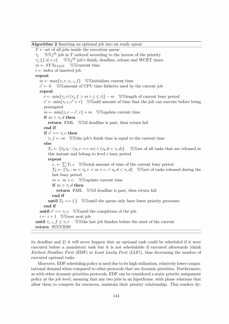
Algorithm 2 Inserting an optional job into an ready queue

T ← set of all jobs inside the execution queueτj %%jth job in T ordered according to the inverse of the priorityτj .f, d, r, c %%jth job’s finish, deadline, release and WCET timesm← SY STIME %%current timei← index of inserted jobrepeat

m← maxτi.r, τi−1.f %%initializes current timec′ ← 0 %%amount of CPU time hitherto used by the current jobrepeat

r ← minτj .r| (τj .f > m ∧ j ≤ i) −m %%length of current busy periodc′ ← minτi.c, c′ + r %%add amount of time that the job can execute before beingpreemptedm← minτi.c− c′, r+m %%update current timeif m > τi.d then

return FAIL %%if deadline is past, then return failend ifif c′ == τi.c then

τi.f ← m %%the job’s finish time is equal to the current timeelse

T1 ← ∀kτk : (τk.r == m) ∧ (τk.d < τi.d) %%set of all tasks that are released atthis instant and belong to level i busy periodrepeat

c ←∑

T1.c %%total amount of time of the current busy periodT2 ← ∀k : m < τk.r < m+ c ∧ τk.d < τi.d %%set of tasks released during thelast busy periodm← m+ c %%update current timeif m > τi.d thenreturn FAIL %%if deadline is past, then return fail

end ifuntil T2 == %%until the queue only have lower priority processes

end ifuntil c′ == τi.c %%until the completion of the jobi← i+ 1 %%test next job

until τi−1.f ≤ τi.r %%the last job finishes before the start of the currentreturn SUCCESS

its deadline and 2) it will never happen that an optional task could be scheduled if it wereexecuted before a mandatory task but it is not schedulable if executed afterwards (thinkEarliest Deadline First (EDF) or Least Laxity First (LLF)), thus decreasing the number ofexecuted optional tasks.

Moreover, EDF scheduling policy is used due to its high utilization, relatively lower compu-tational demand when compared to other protocols that use dynamic priorities. Furthermore,as with other dynamic priorities protocols, EDF can be considered a static priority assignmentpolicy at the job level, meaning that any two jobs in an hiperframe, with phase relations thatallow them to compete for resources, maintain their priority relationship. This renders dy-

144

namic schedulers such as EDF a natural choice for dynamic scheduling that involves changesto the (hiper)frame. Other aspect that favor EDF is its associated large body of knowledge.

Thus, whenever an optional job is released, it checks the state of the execution queue usingthe EDF rules in order to determine if it can enter the queue without causing any job that isalready in the queue to miss its deadline. Nevertheless, as stated before, there may be morethan one job that performs this action and concludes that it is eligible to enter in the queue.In this situation, though the entry of only one task will not cause a deadline miss, the entryof several might. Hence, to solve this problem, first there is a mechanism that introducesprecedences, and second only are inserted in the execution queue the highest precedence jobsthat do not cause a deadline miss of jobs already inside the queue.

The precedence mechanisms are only used when there is a draw concerning which optionaljob enters in the execution queue. Good candidates for precedence mechanisms are those thatwould lead to choices of optional jobs to be executed that increase the overall schedulability,or simply that increase the number of future optional jobs that will be executed. However, forthe best of the author’s knowledge, there is no computationally light algorithm that allows toperform such type of ordering in real-time. Hence, a simple ordering mechanism that consistsin choosing the job from the task set that lost the last arbitration.

Note that the precedence rules are internal to the scheduler. For example, it would betempting to choose, in a control setting with a draw concerning to optional jobs, the jobassociated with a task that had the highest value of some monotonically increasing functionof the error. However, 1) by definition these draws are rare and 2) as seen from the discussionabove if the scheduler has to choose the loser of the previous draw in order to maintainschedulability. It is in this sense that these draws are internal to the scheduler. The onlydraws that do not have these characteristic are the first to happen. However, also by definition,these are even more scarce, too scarce to have a significant impact.

8.3.3 Shifting Mandatory Jobs

As presented in Section 8.3.1, frame changes were bound to happen only in optional jobsthat actually got executed. However, there are scheduling sets in which:

• the task set is schedulable,

• it is impossible to stop jobs from all tasks from being placed as mandatory and releasedsimultaneously,

• whenever jobs from all tasks are released simultaneously at least one deadline is missed.

Such condition can happen, for example, at system startup. Under such conditions, thereis no possible shift of the optional jobs that could possible save the system from missing animportant deadline. A possible solution is to do with mandatory jobs what is also done tooptional ones. Namely,

• whenever mandatory jobs are released, check if all mandatory jobs can be executed,

• if not, sort them according to a predefined set of parameters and the top jobs (accordingto the referred order) are executed as mandatory, the rest act as optional jobs,

• if a mandatory job is not executed, the leftmost bits of its (m, k)–firm frame are rotated.

145

[· · ·

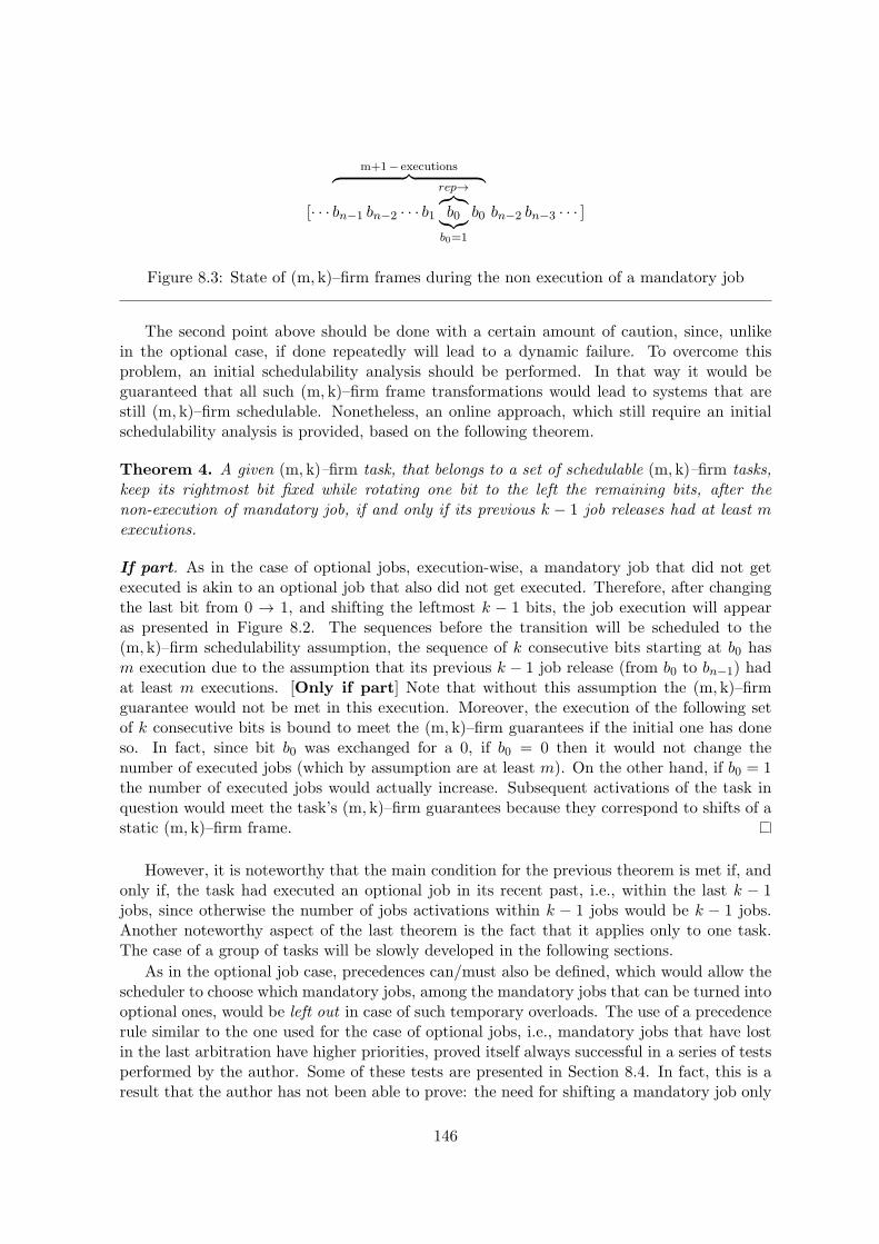
m+1− executions︷︸︸︷bn−1 bn−2 · · · b1

rep→︷︸︸︷b0︸︷︷︸

b0=1

b0 bn−2 bn−3 · · · ]

Figure 8.3: State of (m, k)–firm frames during the non execution of a mandatory job

The second point above should be done with a certain amount of caution, since, unlikein the optional case, if done repeatedly will lead to a dynamic failure. To overcome thisproblem, an initial schedulability analysis should be performed. In that way it would beguaranteed that all such (m, k)–firm frame transformations would lead to systems that arestill (m, k)–firm schedulable. Nonetheless, an online approach, which still require an initialschedulability analysis is provided, based on the following theorem.

Theorem 4. A given (m, k)–firm task, that belongs to a set of schedulable (m, k)–firm tasks,keep its rightmost bit fixed while rotating one bit to the left the remaining bits, after thenon-execution of mandatory job, if and only if its previous k − 1 job releases had at least mexecutions.

If part. As in the case of optional jobs, execution-wise, a mandatory job that did not getexecuted is akin to an optional job that also did not get executed. Therefore, after changingthe last bit from 0 → 1, and shifting the leftmost k − 1 bits, the job execution will appearas presented in Figure 8.2. The sequences before the transition will be scheduled to the(m, k)–firm schedulability assumption, the sequence of k consecutive bits starting at b0 hasm execution due to the assumption that its previous k − 1 job release (from b0 to bn−1) hadat least m executions. [Only if part] Note that without this assumption the (m, k)–firmguarantee would not be met in this execution. Moreover, the execution of the following setof k consecutive bits is bound to meet the (m, k)–firm guarantees if the initial one has doneso. In fact, since bit b0 was exchanged for a 0, if b0 = 0 then it would not change thenumber of executed jobs (which by assumption are at least m). On the other hand, if b0 = 1the number of executed jobs would actually increase. Subsequent activations of the task inquestion would meet the task’s (m, k)–firm guarantees because they correspond to shifts of astatic (m, k)–firm frame.

However, it is noteworthy that the main condition for the previous theorem is met if, andonly if, the task had executed an optional job in its recent past, i.e., within the last k − 1jobs, since otherwise the number of jobs activations within k − 1 jobs would be k − 1 jobs.Another noteworthy aspect of the last theorem is the fact that it applies only to one task.The case of a group of tasks will be slowly developed in the following sections.

As in the optional job case, precedences can/must also be defined, which would allow thescheduler to choose which mandatory jobs, among the mandatory jobs that can be turned intooptional ones, would be left out in case of such temporary overloads. The use of a precedencerule similar to the one used for the case of optional jobs, i.e., mandatory jobs that have lostin the last arbitration have higher priorities, proved itself always successful in a series of testsperformed by the author. Some of these tests are presented in Section 8.4. In fact, this is aresult that the author has not been able to prove: the need for shifting a mandatory job only

146

occur in the first jobs of a task, either at the beginning of the executions or when a new taskis introduced in the task set.

The last three paragraphs suggest an alternative view of the dynamic algorithm presentedherein, namely

1 initialize the execution set with k bits in which m bits are set,

2 if the non-execution of a job would jeopardize the (m, k)–firm guarantees (among thelast k − 1 jobs only m − 1 jobs were executed), set it as mandatory k and set it asoptional otherwise,

3 optional jobs compete for the execution in unused spaces,

4 if a draw occur, when the precedence rule is applied, the task that won the last arbi-tration loses the current one,

5 if a draw remains, choose jobs for execution randomly.

8.3.4 hiperframe Initialization

Dynamic (m, k)–firm scheduling has a number of peculiarities that are nonexisting instatic (m, k)–firm scheduling. For instance, in the static case the hiperframe is known apriori, i.e., before the activation of the first job. A naıve approach would be to initialize thedynamic scheduler with a statical hiperframe that was known to have reasonable schedulingcharacteristics. But the knowledge of such hiperframe implies some sort of static scheduling,which defeats the purpose of using a dynamic scheduler.

In spite of this aspect, the dynamic approach is still of use, because if the task set isschedulable then the dynamical approach converges to an hiperframe that is schedulableregardless of the initial hiperframe. However, it is possible that there is more than onepossible schedule that verifies of (m, k)–firm conditions, some of them differing only in theirphases. Moreover, different initial hiperframes may converge to different final hiperframes.

This is a positive aspect of this scheduler, and of dynamical schedulers in general, namelythere is no need to find an offline schedule. Hence, it suffices to guarantee that the task setis schedulable.

Regarding the initialization per se, as stated before, it is not known a priori any schedu-lable hiperframe. More precisely, for operations like the postponement of a mandatory job, aspreviously discussed, it is vital to already know the (m, k)–firm frame of the job in question.Therefore, measures are necessary to ensure that such initial lack of knowledge will not turninto a dynamic failure in an otherwise (m, k)–firm schedulable set.

One way of achieving such goal is to assume that all previous jobs, of tasks that havenot yet activated any jobs, were successfully executed. This ensures that at the beginning ofthe hiperframe all possible transformations are allowed. However, from an execution point-of-view, being able to execute such jobs even while having to change the initial hiperframe is akinto start from a correct hiperframe and execute the same jobs. Hence, by assuming that alljobs before the beginning of the hiperframe were executed the hiperframe will automaticallyact as or converge to a correct hiperframe.

The strategy presented in the last paragraph is, in a sense, optimal but not unique.For example, the phases of the hiperframe can be used to develop several variations of thepresented strategy.

147

8.4 Examples of Dynamic Scheduling

This section presents a few examples of the execution of the dynamic scheduler presentedin this chapter. These examples are intended, primarily, to give an impression of how thescheduler works. The first group of examples can be scheduled by a static scheduler but it wasincluded because it is helpful to understand how the scheduler works. The second group ismore complex, and presents task sets that are not schedulable by any static scheduler hithertoin the literature, though, subsequent sections of this chapter present a static (m, k)–firmscheduler that is capable of scheduling these task sets. Furthermore, these examples showsome emerging properties of the dynamic scheduler.

Whenever necessary, (m, k)–firm tasks will be described as (C, T,m, k) were the first twovariables designate the worst case execution time and the period respectively.

First, consider a system with two tasks, with the same period and execution time, whichin turn are equal to each other (C = T ) and with a (1, 2)–firm frame. This is a system thatis not schedulable by the scheduler presented in [Ram99], though there are static schedulersthat are able to find a suitable schedule, for example [QH00]. As pointed out in the previoussection, since it is schedulable, the system will converge to an hiperframe that meets all(m, k)–firm guarantees. In so being, lets assume that both tasks start with the (m, k)–firmframe [0 1], which leads to a non schedulable hiperframe. At the start both tasks generatewhat supposedly would be mandatory jobs. Moreover, both jobs can be turned into optionalones, since it is assumed that jobs generated before the start of the hiperframe were allexecuted. Hence, failing this particular job would still meet the (m, k)–firm guarantee, withthe past assumed as have been executed and the current as failed. Using the rules for draws,one job would be chosen randomly for execution and it would maintain its mandatory status,whereas the other would switch to optional as previously described. For the sake of thepresentation, lets assume that the first task kept its first job as mandatory. It is easy to showthat these tasks would never change their (m, k)–firm frames again, repeating themselves asτ1 : [0 1 · · · ] and τ2 : [1 0 · · · ]. Note that the other possible (m, k)–firm hiperframe, accordingto the random choice that is made, differs from the presented choice only in its phase.

For the second example consider also a system with two tasks, namely (1, 1, 1, 2) and(1, 1, 1, 3). Assume that they would start with the (m, k)–firm frames [0 1] and [0 0 1] respec-tively, which are the frames that are generated by the scheduler in [Ram99]. A summarized

1 00 1 1 0 1 00 1 0 1 0 11 0

0 0 1 0 0 1 0 1 0 1 0 0 0 1 0 1 0 0 0 0 1 0 1 0

time

Figure 8.4: A possible schedule of example 2 generated by the dynamic scheduler proposedin this document.

148

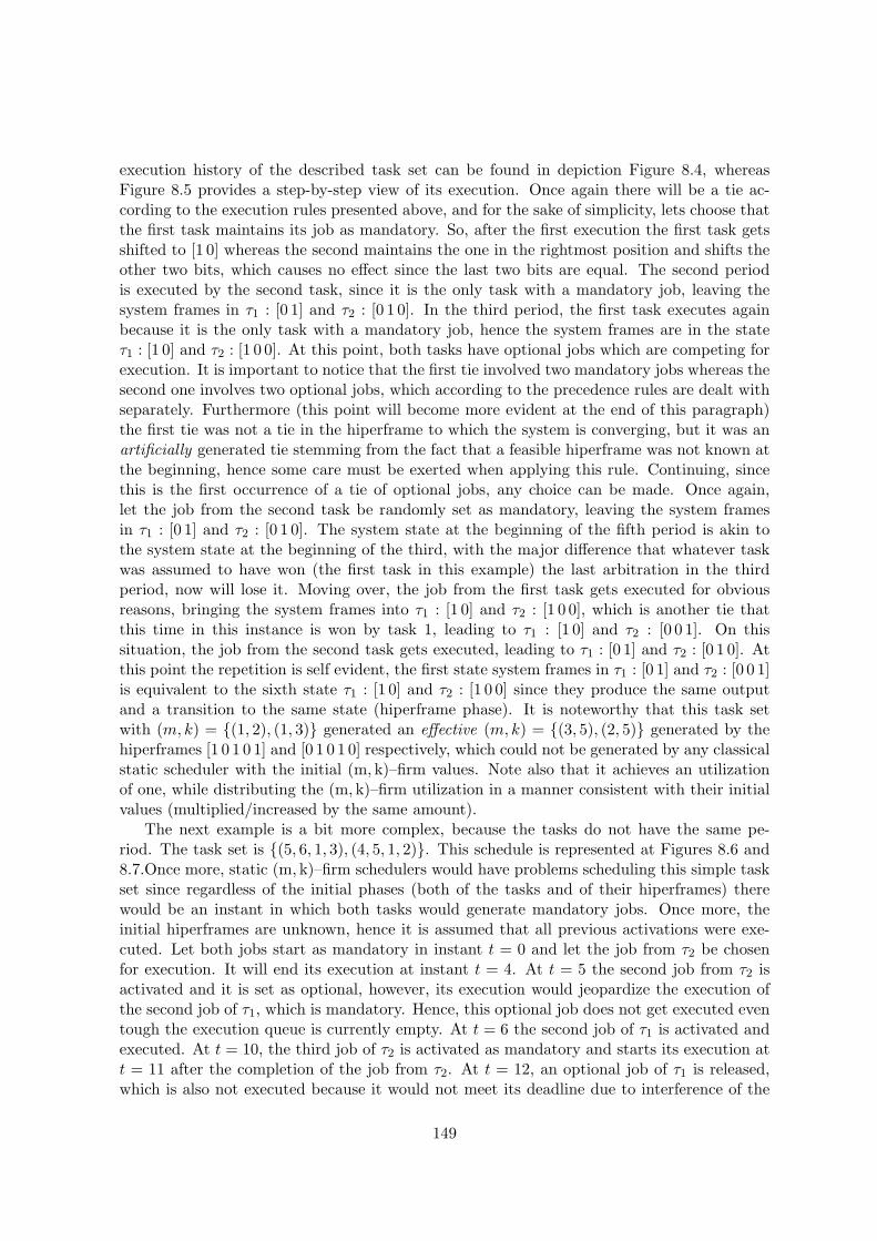
execution history of the described task set can be found in depiction Figure 8.4, whereasFigure 8.5 provides a step-by-step view of its execution. Once again there will be a tie ac-cording to the execution rules presented above, and for the sake of simplicity, lets choose thatthe first task maintains its job as mandatory. So, after the first execution the first task getsshifted to [1 0] whereas the second maintains the one in the rightmost position and shifts theother two bits, which causes no effect since the last two bits are equal. The second periodis executed by the second task, since it is the only task with a mandatory job, leaving thesystem frames in τ1 : [0 1] and τ2 : [0 1 0]. In the third period, the first task executes againbecause it is the only task with a mandatory job, hence the system frames are in the stateτ1 : [1 0] and τ2 : [1 0 0]. At this point, both tasks have optional jobs which are competing forexecution. It is important to notice that the first tie involved two mandatory jobs whereas thesecond one involves two optional jobs, which according to the precedence rules are dealt withseparately. Furthermore (this point will become more evident at the end of this paragraph)the first tie was not a tie in the hiperframe to which the system is converging, but it was anartificially generated tie stemming from the fact that a feasible hiperframe was not known atthe beginning, hence some care must be exerted when applying this rule. Continuing, sincethis is the first occurrence of a tie of optional jobs, any choice can be made. Once again,let the job from the second task be randomly set as mandatory, leaving the system framesin τ1 : [0 1] and τ2 : [0 1 0]. The system state at the beginning of the fifth period is akin tothe system state at the beginning of the third, with the major difference that whatever taskwas assumed to have won (the first task in this example) the last arbitration in the thirdperiod, now will lose it. Moving over, the job from the first task gets executed for obviousreasons, bringing the system frames into τ1 : [1 0] and τ2 : [1 0 0], which is another tie thatthis time in this instance is won by task 1, leading to τ1 : [1 0] and τ2 : [0 0 1]. On thissituation, the job from the second task gets executed, leading to τ1 : [0 1] and τ2 : [0 1 0]. Atthis point the repetition is self evident, the first state system frames in τ1 : [0 1] and τ2 : [0 0 1]is equivalent to the sixth state τ1 : [1 0] and τ2 : [1 0 0] since they produce the same outputand a transition to the same state (hiperframe phase). It is noteworthy that this task setwith (m, k) = (1, 2), (1, 3) generated an effective (m, k) = (3, 5), (2, 5) generated by thehiperframes [1 0 1 0 1] and [0 1 0 1 0] respectively, which could not be generated by any classicalstatic scheduler with the initial (m, k)–firm values. Note also that it achieves an utilizationof one, while distributing the (m, k)–firm utilization in a manner consistent with their initialvalues (multiplied/increased by the same amount).

The next example is a bit more complex, because the tasks do not have the same pe-riod. The task set is (5, 6, 1, 3), (4, 5, 1, 2). This schedule is represented at Figures 8.6 and8.7.Once more, static (m, k)–firm schedulers would have problems scheduling this simple taskset since regardless of the initial phases (both of the tasks and of their hiperframes) therewould be an instant in which both tasks would generate mandatory jobs. Once more, theinitial hiperframes are unknown, hence it is assumed that all previous activations were exe-cuted. Let both jobs start as mandatory in instant t = 0 and let the job from τ2 be chosenfor execution. It will end its execution at instant t = 4. At t = 5 the second job from τ2 isactivated and it is set as optional, however, its execution would jeopardize the execution ofthe second job of τ1, which is mandatory. Hence, this optional job does not get executed eventough the execution queue is currently empty. At t = 6 the second job of τ1 is activated andexecuted. At t = 10, the third job of τ2 is activated as mandatory and starts its execution att = 11 after the completion of the job from τ2. At t = 12, an optional job of τ1 is released,which is also not executed because it would not meet its deadline due to interference of the

149

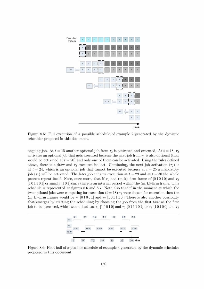
1 0

10

1

01001001

0101010

1 0

00

1

10010010

0101010

1

00

0

10010

10101

1

10

0

01

10

0

10

1

1 1121112 2 2

0 0 1

0 1 0

1 0

1 0

Execution

Pattern

time

Figure 8.5: Full execution of a possible schedule of example 2 generated by the dynamicscheduler proposed in this document.

ongoing job. At t = 15 another optional job from τ2 is activated and executed. At t = 18, τ2activates an optional job that gets executed because the next job from τ1 is also optional (thatwould be activated at t = 20) and only one of them can be activated. Using the rules definedabove, there is a draw and τ2 executed its last. Continuing, the next job activation (τ2) isat t = 24, which is an optional job that cannot be executed because at t = 25 a mandatoryjob (τ1) will be activated. The later job ends its execution at t = 29 and at t = 30 the wholeprocess repeat itself. Note, once more, that if τ1 had (m, k)–firm frame of [0 1 0 1 0] and τ2[1 0 1 1 0 1] or simply [1 0 1] since there is an internal period within the (m, k)–firm frame. Thisschedule is represented at figures 8.6 and 8.7. Note also that if in the moment at which thetwo optional jobs were competing for execution (t = 18) τ1 were chosen for execution then the(m, k)–firm frames would be τ1 [0 1 0 0 1] and τ2 [1 0 1 1 1 0]. There is also another possibilitythat emerges by starting the scheduling by choosing the job from the first task as the firstjob to be executed, which would lead to: τ1 [1 0 0 1 0] and τ2 [0 1 1 1 0 1] or τ1 [1 0 1 0 0] and τ2

τ2

τ1

0 0 1

0 1 0 1

0 0 1 0 1 0

1 0

0 1 0

0 1

1 0 0

1 0 1 0

1 0 0

1 0

0 30252015105

idle

time

Figure 8.6: First half of a possible schedule of example 3 generated by the dynamic schedulerproposed in this document

150

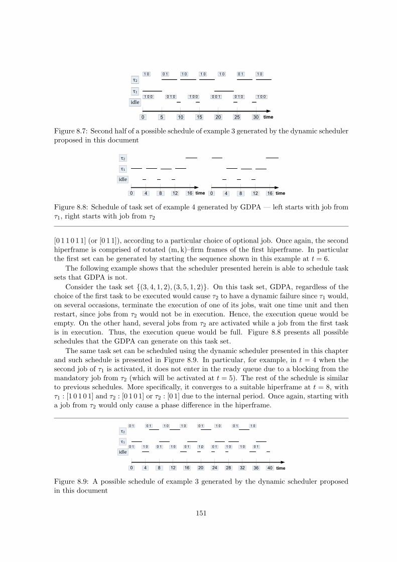
τ2

τ1

1 0 0

1 0

0 1 0

0 1 0 1

1 0 0

1 0 1 0

0 0 1

1 0 1 0

0 1 0 1 0 0

0 30252015105 time

idle

Figure 8.7: Second half of a possible schedule of example 3 generated by the dynamic schedulerproposed in this document

τ2

τ1

0 161284 time

idle

0 161284 time

Figure 8.8: Schedule of task set of example 4 generated by GDPA — left starts with job fromτ1, right starts with job from τ2

[0 1 1 0 1 1] (or [0 1 1]), according to a particular choice of optional job. Once again, the secondhiperframe is comprised of rotated (m, k)–firm frames of the first hiperframe. In particularthe first set can be generated by starting the sequence shown in this example at t = 6.

The following example shows that the scheduler presented herein is able to schedule tasksets that GDPA is not.

Consider the task set (3, 4, 1, 2), (3, 5, 1, 2). On this task set, GDPA, regardless of thechoice of the first task to be executed would cause τ2 to have a dynamic failure since τ1 would,on several occasions, terminate the execution of one of its jobs, wait one time unit and thenrestart, since jobs from τ2 would not be in execution. Hence, the execution queue would beempty. On the other hand, several jobs from τ2 are activated while a job from the first taskis in execution. Thus, the execution queue would be full. Figure 8.8 presents all possibleschedules that the GDPA can generate on this task set.

The same task set can be scheduled using the dynamic scheduler presented in this chapterand such schedule is presented in Figure 8.9. In particular, for example, in t = 4 when thesecond job of τ1 is activated, it does not enter in the ready queue due to a blocking from themandatory job from τ2 (which will be activated at t = 5). The rest of the schedule is similarto previous schedules. More specifically, it converges to a suitable hiperframe at t = 8, withτ1 : [1 0 1 0 1] and τ2 : [0 1 0 1] or τ2 : [0 1] due to the internal period. Once again, starting witha job from τ2 would only cause a phase difference in the hiperframe.

τ2

τ1

0 1 0 1 1 0 1 01 0 0 1 0 1

0 20161284

idle

time24 28 36 4032

1 0

0 11 01 00 11 00 11 00 11 00 1 f

Figure 8.9: A possible schedule of example 3 generated by the dynamic scheduler proposedin this document

151

8.5 Comparison with Previous Solutions

The work presented herein improves upon previous schedulers, as described in Section3.3.1, because it is not bound to EDF-schedulable task sets. The presented work is animprovement even over the work in [QH00], which searched over all possible static frames ofeach task with the corresponding values of m and k, i.e., for each (mi, ki)–firm task it wassearched for all possible ki bits long frame which contained mi ones. This implies that thepresented algorithm outperforms any static algorithm of this family. The following theoremprovides a formal proof of this fact.

Theorem 5. The set of (m, k)–firm task sets that can be scheduled by classical static sched-ulers in which m and k of the (m, k)–firm frames are equal to the respective values of the(m, k)–firm task, is a proper subset of the set of (m, k)–firm task sets that can be scheduled bythe dynamic scheduler presented herein.

Proof. The theorem is true if all (m, k)–firm task sets that can be scheduled by a staticscheduler can also be scheduled by the novel scheduler, i.e., the meaning of the subset part,and there is at least one task set that is schedulable by the proposed scheduler but it isnot schedulable by any static scheduler, implying proper subset part. The subset part ofthe proof can be established if one considers that 1) if there is a static (m, k)–firm schedulethat meets all (m, k)–firm guarantees using (m, k)–firm frames with values of m and k equalto the respective values of the (m, k)–firm, then if the dynamic scheduler is initialized withthe aforementioned schedule (hiperframe), in the worst case scenario, i.e., no optional job isexecuted, the dynamic scheduler will send exactly the same sequence of jobs into the executionqueue. And 2) as discussed above, regardless of the initial schedule (hiperframe), if the task setis schedulable, then the hiperframe converges into a schedulable (fixed) hiperframe, possiblythe static schedule in question. From what follows that if a classical static scheduler can meetall guarantees, so can the dynamic scheduler. For proving the proper part it suffices to presentan example of a task set that is schedulable by the dynamic scheduler but is not schedulableby any classical static scheduler. To this end, consider a task set with two tasks, for which theclassical utilization, i.e., U =

∑iCiTi, is greater than one, with periods that are not multiples

of one another and with implicit deadlines. Consider also, that their (m, k)–firm propertiesare chosen in such a that it would allow the dynamic scheduler to meet its deadlines, for

instance mi = 1 and ki = 2⌈Tj

Ti

⌉, where j represents the other task. Due to the fact that the

periods are not multiples of each other, when scheduled by a stationary scheduler, there willbe an instant in which both tasks are activated as mandatory. At such instant at least one ofthe tasks will fail its deadline since the combined utilization of both tasks is greater than one.Therefore no static scheduler can guarantee that the (m, k)–firm constraints will be met. Onthe other hand this task set is schedulable by the dynamic scheduler by construction. Thiscompletes the proof.

An important remark is that classical static (m, k)–firm schedulers can only schedule tasksets that are EDF schedulable (see discussion at the beginning of this section) and all EDFschedulable task sets are schedulable by the dynamical algorithm proposed here, since theexecution queue is itself EDF scheduled. Furthermore, besides the point raised by the lasttheorem about the set of schedulable task sets, it is important to realize that even amongthe task sets for which there is a classical static schedule, the proposed scheduler achieves

152

mandatory

optional

Figure 8.10: Example of an advantage of a single queue.

utilizations that are never inferior. In fact, they are usually higher than those achieved byclassical statical schedulers.

A major difference, which is also an improvement, between the approach presented hereand classical static (m, k)–firm schedulers, is the fact that in the classical approaches theschedulers have two queues, namely: queue 1, devoted to mandatory jobs, and all jobs thatare in it get scheduled; queue 2, is used to schedule optional jobs, and these jobs are onlyexecuted if queue 1 is empty. Each queue is scheduled according to classic scheduling policies,such as EDF. In the approach proposed in this chapter, it is used only one queue. This in turnmay increase the number of optional jobs that are executed. For example, consider Figure8.10, in which the mandatory job has an absolute deadline that is rather far away, whereasthere is an optional job that has a deadline that is relatively near. In the scheme that is usedin classical static/dynamic (m, k)–firm schedulers, the mandatory job would be in the highestpriority queue, hence it would be executed first. Thus, the optional job would not be executedright away because the mandatory job was already in execution, leading to a deadline missof the optional job. On the other hand, in the proposed scheduler, after certifying itself thatthe optional job would not cause a deadline miss, would execute the optional job, as shownin Figure 8.10, hence meeting the deadline of both jobs.

But there are a few downturns. The first is related to the high computational complexityof the proposed dynamic scheduler. A related negative aspect, which is also common toall dynamic algorithms, deals with the loss of predictability under overload conditions. Byoverload it is meant the moments in which the task set is not schedulable. The loss ofpredictability occurs in the sense that in scheduling algorithms such as those presented in[Ram99], whenever there is a violation of an (m, k)–firm guarantee, the tasks with the longestperiods suffer the violation. Since on such schedulers the initial instant is a critical instant,due to the fact that in such instant all tasks activate a job set as mandatory, and jobs in theexecution queue are served in a Rate Monotonic manner. Furthermore, when a job misses amandatory job it also violates its (m, k)–firm guarantee. On the other hand, for the case ofdynamic (m, k)–firm schedulers, it is not possible to make such predictions beforehand.

The work presented in this chapter improves upon the work of DBP and its variantsbecause it does not have any of the downturns presented in the section 3.3.1. Examples ofsuch downturns include a disregard for the deadlines of the tasks, the fact that the algorithmtends to schedule tasks with a short distance to failure close to each other, a total disregardfor the relation of the periods of the tasks (this point will become clearer in the next section)and a disregard for the relations between the time to failure of the various tasks.

A third negative aspect of the use of dynamic (m, k)–firm schedulers, relates to the factthat some applications require that beside the usual (m, k)–firm guarantees, tasks must havea mandatory job in a pre-determined part of the (m, k)–firm frame. Examples of these ap-

153

plications include the JPEG frame transmission, as discussed in the Section 3.3.1. Undersuch conditions, a dynamical scheduler, as presented so far, can not give all guarantees dueto the loss of predictability that was already discussed. Nevertheless, it is possible to makesome modifications in order to properly accommodate these requirements, such as splittingthe task, giving different values of m and k to each of the subtasks, one or more behaving asa classical task, i.e., executing all of its jobs. Or modify the (m, k)–firm definitions as to havethree levels of jobs instead of the current two, i.e., mandatory and optional.

8.6 Static (m,k)-firm frames (Revisited)

In the previous section it was established that the dynamic (m, k)–firm scheduler pre-sented here can schedule tasks sets that otherwise cannot be scheduled by classical (m, k)–firmschedulers. This may seem paradoxical since, for example, the approach presented in [QH00](theoretically) searches through all possible (m, k)–firm (meta) frames.

However, there is no paradox. In fact, the apparent contradiction stems from the set of as-sumptions that were made about the space of (m, k)–firm frames that meet a given (m, k)–firmguarantee. That is, at the beginning of this chapter it was shown that any repetition pattern,with k bits of which (at least) m, i.e., frame, generate a mandatory job sequence that fulfilledthe respective (m, k)–firm guarantees. The contradiction appears when it is assumed thatthis is the only way of generating sequences that provide (m, k)–firm guarantees in question.In fact, there are other repeating sequences that also generate (m, k)–firm sequences withsimilar guarantees.

For example, recalling the sequence that was given in the first example, i.e., an (1, 2)–firmtask had the generating (m, k)–firm frame [1 0 1 0 1] which always meet the (1, 2)–firm guar-antee.

Thereby, the space of all possible (m, k)–firm frames that give a certain (m, k)–firm guar-antee does not only include all possible (m, k)–firm frames withm and k having values equal tothose of the respective (m, k)–firm, but it includes all (m′, k′)–firm frames that when repeated(indefinitely) generate a sequence in which any subsequence of k consecutive activations con-tains at least m jobs that are executed. In the remaining of this section a number of propertiesof such sequences will be presented, but first an important definition is in order.

Definition. An infinite sequence of (m, k)–firm job activations is tight if for every set of kconsecutive activations there are exactly m executed jobs.

The concept of tight sequences, though simple, helps to visualize other concepts relatedwith (m, k)–firm frames and sequences. In fact, in a nutshell, the concept of tight sequencesencapsulates most of the contributions in the literature regarding static (m, k)–firm schedul-ing. But more importantly, it helps to give a view of other possible (m, k)–firm schedulers.

Theorem 6. An (m, k)–firm sequence is tight if and only if it exists an (m, k)–firm framewith the same values of m and k that can generate it.

Proof. The basics for the proof was already given in previous discussions. The if part, whichseeks to establish that using the aforementioned type of frames generates the sequences inquestion, is easy to establish: In fact, it was proved in Theorem 1. The only if part, whichaims at proving that this type of sequences can be produced only by the claimed type offrames, is proven because if a sequence is tight then whenever the last kth job is/was executed

154

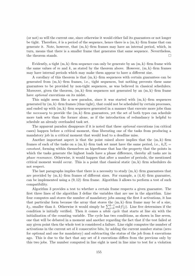
(or not) so will the current one, since otherwise it would either fail its guarantees or not longerbe tight. Therefore, k is a period of the sequence, hence there is a (m, k)–firm frame that cangenerate it. Note, however, that (m, k)–firm frames may have an internal period, which, inturn, means that there is a smaller frame that generates that same sequence. Nevertheless,the theorem stands.

Evidently, a tight (m, k)–firm sequence can only be generate by an (m, k)–firm frame withthe same values of m and k, as stated by the theorem above. However, (m, k)–firm framesmay have internal periods which may make them appear to have a different size.

A corollary of this theorem is that (m, k)–firm sequences with certain guarantees can begenerated from (m, k)–firm frames, i.e., tight sequences, but nothing prevents these sameguarantees to be provided by non-tight sequences, as was believed in classical schedulers.Moreover, given the theorem, (m, k)–firm sequences not generated by an (m, k)–firm framehave optional executions on its midst.

This might seem like a new paradox, since it was started with (m, k)–firm sequencesgenerated by (m, k)–firm frames (thus tight), that could not be scheduled by certain processes,and ended up with (m, k)–firm sequences generated in a manner that execute more jobs thanthe necessary to provide the (m, k)–firm guarantees, yet the set of both types can schedulemore task sets than the former alone, as if the introduction of redundancy is helpful toschedule an already overloaded task set.

The apparent paradox disappears if it is noted that these optional executions (on criticalcases) happen before a critical moment, thus liberating one of the tasks from producing amandatory job in a critical moment that would lead to a deadline miss.

Another important aspect is that the point raised above implies that the (m, k)–firmframes of each of the tasks on a (m, k)–firm task set must have the same period, i.e., kiTi =constant, forming within themselves an hiperframe that has the property that the points inwhich the tasks generate the highest loads have a phase difference, thereby all tasks are inphase resonance. Otherwise, it would happen that after a number of periods, the mentionedcritical moment would occur. This is a point that classical static (m, k)–firm schedulers donot respect.

The last paragraphs implies that there is a necessity to study (m, k)–firm guarantees thatare provided by (m, k)–firm frames of different sizes. For example, a (4, 6)–firm guarantee,can be implemented using a (9, 12)–firm frame. Algorithm 3 allows to perform a test of suchcompatibility.

Algorithm 3 provides a test to whether a certain frame respects a given guarantee. Thefirst three lines of the algorithm 3 define the variables that are use in the algorithm. Linefour computes and stores the number of mandatory jobs among the first k activations, it hasthat particular form because the array that stores the (m, k)–firm frame may be of a size,kf , smaller than k. Otherwise it would simply be

∑k−1j=0 mkf(j). Line five determines if the

condition is initially verified. Then it comes a while cycle that starts at line six with theinitialization of the counting variable. The cycle has two conditions, as shown in line seven,one that will be debated in a moment and another regarding the fact that if the test failed atany given point then the whole test is considered a failure. Line eight computes the number ofactivations in the current set of k consecutive bits, by adding the current number status (zerofor optional and one for mandatory) and subtracting the status of the job from k executionsago. This is due to the fact that any set of k executions differs from the previous only bythis two jobs. The number computed in line eight is used in line nine to test for a violation

155

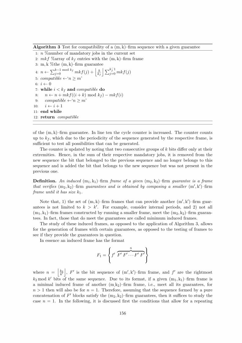
Algorithm 3 Test for compatibility of a (m, k)–firm sequence with a given guarantee

1: n %number of mandatory jobs in the current set2: mkf %array of kf entries with the (m, k)–firm frame3: m, k %the (m, k)–firm guarantee

4: n←∑k−1 mod kf

j=0 mkf(j) +⌊

kkf

⌋∑k−f 1

j=0 mkf(j)

5: compatible←‘n ≥ m’6: i← 07: while i < kf and compatible do8: n← n+mkf((i+ k) mod kf )−mkf(i)9: compatible←‘n ≥ m’

10: i← i+ 111: end while12: return compatible

of the (m, k)–firm guarantee. In line ten the cycle counter is increased. The counter countsup to kf , which due to the periodicity of the sequence generated by the respective frame, issufficient to test all possibilities that can be generated.

The counter is updated by noting that two consecutive groups of k bits differ only at theirextremities. Hence, in the sum of their respective mandatory jobs, it is removed from thenew sequence the bit that belonged to the previous sequence and no longer belongs to thissequence and is added the bit that belongs to the new sequence but was not present in theprevious one.

Definition. An induced (m1, k1)–firm frame of a given (m2, k2)–firm guarantee is a framethat verifies (m2, k2)–firm guarantees and is obtained by composing a smaller (m′, k′)–firmframe until it has size k1.

Note that, 1) the set of (m, k)–firm frames that can provide another (m′, k′)–firm guar-antees is not limited to k > k′. For example, consider internal periods, and 2) not all(m1, k1)–firm frames constructed by running a smaller frame, meet the (m2, k2)–firm guaran-tees. In fact, those that do meet the guarantees are called minimum induced frames.

The study of these induced frames, as opposed to the application of Algorithm 3, allowsfor the generation of frames with certain guarantees, as opposed to the testing of frames tosee if they provide the guarantees in question.

In essence an induced frame has the format

F1 =

f ′

n︷︸︸︷F ′ F ′ · · ·F ′ F ′

where n =

⌊k2k′

⌋, F ′ is the bit sequence of (m′, k′)–firm frame, and f ′ are the rightmost

k2mod k′ bits of the same sequence. Due to its format, if a given (m1, k1)–firm frame isa minimal induced frame of another (m,k2)–firm frame, i.e., meet all its guarantees, forn > 1 then will also be for n = 1. Therefore, assuming that the sequence formed by a pureconcatenation of F ′ blocks satisfy the (m2, k2)–firm guarantees, then it suffices to study thecase n = 1. In the following, it is discussed first the conditions that allow for a repeating

156

frame to satisfy certain guarantees and second the conditions as is to some extent done in thefollowing set of theorems. The following theorem can also be used in other circumstances,namely to make it easier to find new frames that meet some guarantees, given that anotherframe that meets the same guarantees is known.

Theorem 7. Any (m1, k1)–firm frame generated by the repetition of another (m′, k′)–firmframe is an induced frame that satisfies some (m2, k2)–firm guarantees, with k1 > k2 if andonly if 1) (m′, k′)–firm frame satisfies (m2, k2)–firm and 2) every right-going sequence of, up tok1mod k2, consecutive bits starting at bit k1mod k2 counted from the right does not have lessmandatory jobs than a right-going sequence of the same size, starting from the leftmost bit.The case k1 ≡ 0mod k2 is also contained in the last sequence: it would imply a comparison oftwo zero length sequences that cannot have different number of mandatory activations, henceit suffices that (m′, k′)–firm frame satisfied the mkfm2k2 guarantees.

Proof. The first k1 activations (mandatory/optional) of the (m1, k1)–firm frame are exactlythe activations of its generating ((m′, k′)–firm) frame, by construction. Therefore, if any missof the (m2, k2)–firm guarantees occur it will happen during the shift of the k1≡ 0 (mod k2),i.e., when the set of last k2 consecutive bits have at its left p (p < k2) bits of which wherethe rightmost bits of the (m′, k′)–firm frame and at its right k2 − p also from the rightmostbits from the (m2, k2)–firm frame. Upon such shifts, the set of the last consecutive bits willhave a number of the rightmost bits of the initial (m′, k′)–firm. Since the initial sequence wastight (by construction), it will maintain its guarantee if and only if the bits that replaced theoriginal bits of the sequence do not have less ones than the original.

A corollary of the previous theorem is that, if at any point the number of ones of thereplacing sequence, i.e., the sequence that starts at bit k1mod k2 (counted from the right), isgreater than that of the sequence being replaced, then at such point, the respective sequenceof last k2 consecutive bits will have more than m2 bits, thus its sequence that is generatedwill not be tight. Conversely, if it is smaller, then at the point in question the respectivesequence will be in a dynamic failure.

For example, borrowed from the second example above, assuming that m =⌈k2

⌉, the

frame [1 0] only generates minimum induced frames if the new frames have an even k, sinceotherwise the leading zero would conflict with the trailing one. On the other hand, the frame[0 1] always generates a minimum induced frame. In particular the solution presented at thetime (generated by the dynamic scheduler) is not unique. Another solution is τ1:[0 1 0 1 0 1]and τ2:[1 0 1 0 1 0] (and a shift of one bit of the hiperframe), which is generated for k1 = 2 theinitial frames τ1:[0 1] and τ2:[1 0]. Note that for tau2, k1 < k2.

It should be remarked that a shifted version of an induced frame that satisfies a given(m, k)–firm guarantee, also satisfies the guarantees in question. This point becomes of utter-most importance when building static hiperframes, in which each of individual frame was builtfrom a smaller (m, k)–firm, but the frames must have a phase relation between themselves asdiscussed above. Nevertheless, regarding the phase of inducing frame, i.e., the smaller one,its phase, also as discussed above, does change whether or not the resulting frame providesthe intended guarantees.

The following is another corollary of the previous theorem, which is essential to under-stand the relationship between static and dynamically (m, k)–firm frames. But due to itsimportance, it will be stated as a theorem.

157

Theorem 8. If a given (m1, k1)–firm frame satisfies the guarantees of another (m2, k2)–firm,then after extending the repeating (m1, k1)–firm frame until it has a size that is a multiple ofk2, the number of mandatory jobs will be no smaller than m2 ·gcd(k1, k2), with gcd being the‘greatest common divider’.

Proof. The proof is rather simple, since if the number of mandatory jobs were smaller thanm2 · gcd(k1, k2), then it would imply that at some point of the extended frame it wouldviolate the (m2, k2)–firm guarantees, which contradicts the assumptions that (m1, k1)–firmframe satisfies the guarantees of (m2, k2)–firm.

Note that being non-smaller implies that either their is a classical (m, k)–firm frame, i.e.,in which k1 = k2, or there will be more executions than necessary, thus implying the executionof optional jobs, as it was postulated beforehand and now is proven.

Summarizing, the dynamic scheduling algorithm presented in previous sections, if leftrunning without any unforeseen events, generates an execution pattern that is similar to theexecution pattern generated by static frames discussed in this section.

8.6.1 Optimal Statical (m,k)-firm Scheduling

This section provided a number of tools that allows one to speak about optimal (m, k)–firmscheduling. In special, now searches of all possible hiperframes that respect a given set of(m, k)–firm guarantees are possible. This section is intended to provide rules to guide such asearch.

The minimum induced (m1, k1)–firm frame is, as implied by its name, the frame of size kthat has the minimum number of mandatory jobs and is generated by a given (m′, k′)–firmframe, while meeting a given (m2, k2)–firm guarantees. Due to such minimality, if there is anypossible schedule then, there is a way of scheduling it using only minimum induced (m, k)–firmframes.

The hiperframe has a period that is also a period of all of its tasks. Thereby, it onlymakes sense to test the (m, k)–firm (each task) in which k is equal to the hiperframe, that is,of common multiples of all tasks periods. Furthermore, only initial (m′, k′)–firm frames thatgenerate appropriated minimum induced (m, k)–firm frames need to be tested, even though,for each set of minimum induced frames all possible phases will have to be tested.

8.7 Conclusion

(m, k)–firm schedulers have a great potential to improve the performance of many real-timeapplications. However, for many application, improvements cannot occur until it is possibleto provide some deterministic guarantees regarding the performance of the schedulers.

Two avenues for the development of this type of (m, k)–firm schedulers were discussed. Thefirst approach concerned dynamic schedulers, which traditionally has been mostly comprisedby probabilistic schedulers of the DBP family. However, the proposed dynamic schedulerhinged upon the fact that it is possible to dynamical change an (m, k)–firm frame whilemaintaining its respective guarantee. In fact, there are task sets in which only is possible toprovide the respective guarantees if the respective frame is changed at some point.

A second scheduler was discussed, in this case a static one, and it was based on the factthat the frame that a given (m, k)–firm task used to schedule a given task did not need to

158

be k bits long with m ones. In fact, it was shown that it is possible to provide the sameguarantees using frames of different sizes. Furthermore, there are task sets that cannot bescheduled, in the deterministic sense, using classical approaches, i.e., with frames of sizesequal to the respective (m, k)–firm values, but that can be scheduled by this generalizationof static schedulers.

Notwithstanding the novelty of these two new schedulers, some points remain to be opti-mized. For example, the algorithm for the insertion of a new job on the dynamic schedulers’execution queue, which in its current state is relatively computationally intensive, therebyincreasing the time required to perform a context switch. Another point that needs someimprovement is the schedulability test, since so far it has only been put forth a mechanismthat detects if a given schedule verifies the guarantees but has not been put forth an algorithmto test if it is possible to find a schedule that provides the guarantees.

159

Chapter 9

Aggregation of Duplicate SensitiveSummaries

9.1 Introduction

Previous decades brought about a revolution in radio and microprocessor technology thatmade possible a plethora of new applications. In the midst of such development, WirelessSensor Networks (WSN) have recently emerged as a synergy of two related technologies, i.e.radio and microprocessors. Both of them had exponential improvements in cost, size andfunctionality in recent years. In particular, the possibility of using many inexpensive sensornodes interconnected by WSN for a number of ends, which made possible a novel set ofapplications so diverse as air monitoring, forest fire detection, structural monitoring, watermonitoring, etc. Furthermore, such improvements are expected to keep their pace in the nearfuture, thus WSN should become even more prevalent.

This potential of WSN drew the attention of the research community. This research isfurther motivated by the fact that many aspects of WSN remain as open problems. Problemssuch as the fact that WSN are usually heavily resource-constrained. Of particular relevanceis energy efficiency since, in many applications, nodes have to operate during long periodswithout an external energy source, which made energy conservation one of the most studiedaspect of WSN.

The literature on this topic reveals many techniques to improve energy efficiency, suchas the use of in-network aggregation, the use of clustering (with or without cluster headrotation), exploitation of the inherent spatial correlation of readings among neighbor nodes,variation of transmission energy, sleeping during long periods of inactivity, exploitation oftemporal correlation of the signals (data caching, estimation, system identification and soon), among others.

One approach to data transmission from common nodes to the root, which is of particularrelevance for the present discussion, is to have all nodes transmit their data integrally to theroot and at the root perform the computations on the collected data. However, this approachis energy-wise inefficient due to the rather high number of messages that are sent. A moreefficient approach is the gradual aggregation of values as they are transmitted upstream,which is called in-network aggregation.

On the other hand, WSN links are fragile. Particularly, they can be temporarily unavail-able, be subject to relatively high error rates or be asymmetric, among other issues. Hence,

161

the use of multi-path routing has been proposed [CLKB04, MYH06, MNG05, WW11] tolessen its effects.

However, the problem of aggregation of duplicate sensitive summaries (e.g. sum, average,histogram, etc.) in multi-path routing networks is not fully resolved. In fact, the use ofmulti-path routing may cause errors in the aggregation of duplicate-sensitive functions. Afunction is said to be duplicate-insensitive if its result does not change upon the introductionof a duplicate argument. For example, the min and max functions are duplicate-insensitive. Afunction is said to be duplicate-sensitive if its output changes with the addition of a duplicateargument. For example the sum function, in which introducing a non-zero argument morethan once causes different results, is duplicate-sensitive.

Many attempts have been made to solve this issue, for example, by giving approximateanswers, by forcing single path routes, by searching for aggregate-insensitive versions or bydecomposing these functions in a series of duplicate-insensitive functions and then query theWSN for each of the new functions, among others.

None of the already introduced solutions satisfy the initial goals, since they either havean error by nature (approximations based approaches), or use single routes, which does notoffer any redundancy, or considerable increase the number of messages that are required tocompute the aggregate (alternative functions approaches), thus defeating the original purposeof the aggregation, which is reduce the number of messages to save energy.

This chapter proposes algorithms that address this problem by sending redundant aggre-gated information through different paths, so the data can be reconstructed to obtain thebest possible summary, given the available paths. Two algorithms are presented, one bettersuited for networks dominated by link errors and another better suited to networks where thepredominant error source is node failure. The algorithms are light during normal networkoperation, with the most intensive processing performed during the initialization phase.

The approach presented herein outperform previous solutions found in the literature intwo key aspects: complete topology independence and aggregation depth independence. Thealgorithms are topology independent in the sense that there is no need to manually configurethe topology of the network into the nodes nor is necessary to put the nodes in a pre-specifieddistribution. The algorithms are aggregation depth independent in the sense that they workproperly regardless of the number of levels of the networks.

The remaining of this chapter is organized as follows. Section 9.2 presents an overviewof the related work. Section 9.3 describes the count summary that is used in this chapter.Section 9.4 presents the methodology proposed in this chapter to carry out the aggregate ofduplicate-sensitive data in multi-path networks. Section 9.5 discusses the applicability of theprosed algorithms. Section 9.6 presents simulation results carried out to assess the correctnessof the algorithms and to evaluate its performance. Finally, section 9.7 concludes the chapter.

9.1.1 On the Use of In-Network Aggregation of Duplicate Sensitive Sum-maries for WSN Control Applications

The use of WSN for control processes is booming, due to the ever decreasing cost-performance ratio of the WSN. Furthermore, there are certain industries, e.g. the metallurgic,in which the use of wires is not a viable option for the sensor-controller communication.

However, existent WSN lack a number of functional, and of more relevance for the currentthesis, the error rate guarantees needed to ensure the proper function of a control system.Moreover, these control applications require many spatially distributed, though temporally

162

dense sensor readings.

These facts imply that the current WSN need to be improved in order to deliver suchimprovements. This chapter presents one such improvement that has the potential to makethe goal of using WSN for control applications a reality.

9.2 Related Work

Due the size of the literature of the topic, as can be attested by some reviews as in[CGKL11], the field of WSN is too vast to be covered in a related work topic of a singlechapter. Therefore, this section is intended to give a perspective of the field by presentingonly contributions closely related to the problem addressed in this chapter.

The use of aggregation in WSN excels in metrics such as energy expenditure and networklifetime, as shown in [KEW02]. Furthermore, in the same reference it is also shown that thedenser the network the higher the benefits of aggregation. [KDN02] corroborates with thesefindings. [WMG04] presents a meta-level view of aggregation and argues for a co-design ofthe integrating parts of the network.

TAG [MFHH02] was one of the first contributions to tackle the problem of aggregation inWSN and under it nodes build the network by setting the level of the parent as the lowestlevel that it received and set the sending node(s) as the parent, set its own level as the levelof the parent(s) plus one and broadcast its own address plus its level. [WDAA09] builds atree similar to Shared Resource Tree (SRT) used in TAG (which the authors of TAG callTinyDB), however it is augmented by the use of an index table to decide the aggregationvalue, plus a common value (cv) agreement, which is a value that nodes with the same parentare supposed to verify |nodereading − cv| < δ, cv is computed as the average of the childrenreading and is sent back to them. If a children verifies the last condition then it does notsend its data. max /min are also based on cv, thus may lead to erroneous values. In fact,this aspect is common to approaches that use a cluster head and spatial correlation. Underthis approach, nodes with more than one parent alternate between sending messages to eachof its parents.

In [ZGE03] it is introduced the direct diffusion of digests (aggregates), in which nodescompute their value as a function of their current value and the value received from neighbornodes. They start sending this new value piggy-backed in a periodic beacon of the underlyingcommunication layer, for example, with a heartbeat message. It takes at most the diameterof the network (in number of hops) to diffuse such digests. Obviously, in this form it onlycan compute digests of exemplary functions. Exemplary functions are those that can becomputed as the result of an aggregate of previous values and one single new value. In fact,they have this name because their result depend on only one value, for example max and minsummaries. For non-exemplary functions, the authors propose that, first, a direct digest thatis always won by the sink is performed, second, each node would memorize the node fromwhich it received the winning diffusion (parent) until a tree is formed, third, a diffusion issent along the tree that emerged in the process. All the same, the authors do not showany difference between their proposal and the regular diffusion. Notwithstanding, the paperpresents an interesting study of link asymmetry in WSN, which led the authors to propose amechanism to switch parents whenever a certain link is asymmetric.

In the same line, [NGSA04] provides a formalization of the concept of diffusions. Threeoperations are considered: synopsis generation, fusion and evaluation, that work as suggested

163

by their names. The paper also provides a number of, so called, necessary and sufficient con-ditions for correctness, though, it also presents a situation that verifies all such conditions butdoes not produce the correct value, implying that the presented conditions are not sufficient(their necessity may also be under dispute). [CMV08] uses a fuzzy logic approach to computeexemplary functions. Each node has a fuzzifier that decides whether to send the data. Acomparison with the ‘no aggregation scenario’ was made, though no comparison with classicalaggregations was presented. It was also used the sleep approach.

In [MYH06] it is proposed to solve the problem of multi-path aggregation of duplicatesensitive nodes by keeping nodes from aggregating data if there is a possibility of duplication.To this end, upon the construction of the multi-path tree, nodes send their’s and their parentsaddresses along with their hop count to the root. Nodes that join the network, would knoweach of their parents and their parent’s parents. Based on this information, if the node as morethan one parent, then it chooses the parent’s parent with most paths from it as the aggregationpoint, otherwise it chooses its only parent as the aggregation point. Only two levels of theWSN are searched for, therefore it might happen that the link of the chosen parent’s parentsup the tree may fail while there is another parent’s parents link which is operational. Thefact that the lost of one (up tree) link/node can cause the loss of information of many ofchildren nodes puts in question the very use of multi-path (redundancy). This approachpoint is explored in the approach advocated in this chapter.

In [MNG05] it is used an hybrid approach to routing. Using a tree approach closer to theleaves and a multipath approach closer to the sink. This helps to leverage the advantages oftrees (low latency, low messaging) with the advantages of multipath (increased robustness).Furthermore, it is paramount to have redundancy in nodes that transport the aggregates ofseveral other nodes, nonetheless, the authors approach to the transport of multipath trafficis highly inefficient, since it uses no aggregation. The authors justify their choice by notingthe problems that arise with the use of aggregation in multipath routing, which are the sameproblems that this chapter is set to solve.

The above presented approaches to WSN try to reduce the energy expenditure of WSNby changing the way in which data is routed. But, as discussed in Section 9.1, there areother approaches, such as the use of approximate queries, which require less data to compute.Among the approximate queries (in which SOD based approaches are arguably a member),[GGP+03] uses a wavelet based approximate aggregation technique to store the results ofseveral queries at different network hierarchies. Nodes at different hierarchies store resultswith different precisions. Whenever a query with a certain precision is done, it drills downthe network until it finds a node with enough precision to answer the query. Due to the highvolume of data generated by this approach, an aging scheme was employed.

Considine et al [CLKB04] present the FM-SKETCH (introduced by Flajolet and Martin),which approximate the number of distinct elements of a superset by seeing only its initialpart. In turn, such sketches are used to estimate the number of distinct nodes in a network— approximate count summary — which, the authors argue, is well suited for multi-pathnetworks. The paper generalizes FM-SKETCH to approximate sum summaries by havingeach node producing val (val is the value that the node sensed) distinct elements into thesuperset. Evidently, the number of distinct elements of this superset is equal to the sumsummary. The sum summary is approximated by using the FM-SKETCH on the superset. Anumber of optimizations are provided. All the same, this approach that supposedly reducesthe amount of data by computing approximates, actually for typical relative errors (0.85-0.95), it uses about the same amount of network resources (since it has no aggregation) and

164

computer resources (memory and CPU) as traditional exact summaries (with aggregation).The authors compared their approach to TAG and to the LIST approach, i.e., each nodesends the value of the aggregate and the set of nodes used to compute the aggregate, whichis similar to the approach provided herein, however, their LIST approach is considerable lessoptimal. First, nodes always send a huge set, second the node that is receiving may not becapable of finding a way to properly aggregate the received data due to duplications in thereceived data.

The use of SOD in order to reduce the amount of data that is sent, i.e., the exploitationof temporal correlation, has also been explored in a number of articles, more prominently in[MA01] and later at [MA02] the authors use a hybrid periodic\asynchronous model, in whichdata is sent periodically, however, rapid transitions are responded to by immediately sendingdata asynchronously. [SBLC03] aims at similar goals, using data caching and aggregation ateach level of the tree.

Al-Karaki et al [AKUMK04] present both an exact and an approximate algorithms to findoptimal routes for aggregation in WSN. The exact algorithm is stated as an integer linearprogramming problem, which the authors argue to be too complex to be solved in WSN.Hence, they propose an approximate genetic algorithm. However, the genetic algorithm isitself computationally heavy and involves many message exchanges, which is exacerbated bybeing performed in several rounds, during the normal function of the WSN, thereby consumingthe very same energy that the algorithm aims at saving.

Approximate aggregations for the histogram (HIST) summary have also been proposed, asis the case of quantile tracking [CGMR05, SBAS04], top-k estimation [WXTL06, WXTL07]though the later group tend to be more exact. [AN11] is an example in which an approximationof an histogram is used to compute queries in WSN, however, the algorithm used is exactif the histogram is exact, but the authors do not provide any algorithm to compute exacthistograms.

Aggregation in sparse networks is also an active research topic, motivated the energy sav-ing approaches that put a significant fraction of networks on sleep mode. One such approachis described in [GGMH07], in which a dense WSN with a small number of hotspots is studied.A mechanism to find suitable routes is presented.

Another class of approaches is the bio inspired one, which is epitomized in [LKF07](nonetheless, a similar approach is pursued in [OK09] and in references therein,) leveragesthe (ant) bio-inspired path finding algorithm, to build a routing tree. In this algorithm, allsource nodes explore all paths to the sink, leaving a certain amount of pheromone at each link.Several factors (e.g. path size) determine the amount of pheromone left on each link. Theamount of pheromone on each link is the sum of the amount left by on each paths that goesthrough the link. The higher a path’s pheromone levels, the more likely it will be active. Thisfamily of algorithm has the downside of not being computationally and energetically light,even during normal operation. But have the upside of being extremely optimal at finding thepaths and at reacting to topology changes, though not necessarily fast.

Another type of aggregates that gain a certain moment in the community is the gossipbased aggregation [DSW06, KDG03, SZG07, FLS06, BGPS06, CPX06], in which each node1) read its own value, 2)aggregates it with messages that it receives and 3) sends a messageto a random neighbor with a fraction of its current value while maintaining another fractionof it. After an algorithm-dependent number of rounds, the aggregates converge to the correctvalue. Usual objections include the apparent lack of benefits for the common WSN, higherlatencies and increased number of data exchanges.

165

Other types of optimizations to WSN that are not related to the main contributionof this chapter have been proposed, such as the exploitation of temporal correlation in[OJW03, OLW01, OW02, DKR04, SBS+02, OW00]. And spatial correlation, such as [RKK04,GBT+04, GNDC05, HCB00, DGM+04, JP04, OK09, GGMH07, VA06, YS07].

9.3 Count Summary

The main contribution of this work is independent of the intricacies of the underlyingcount summary. Nevertheless, it requires the execution of a count summary prior to carryingout an aggregation of a duplicate-sensitive function, or at least, to have the results of a countsummary in cache. Therefore, it is paramount to use an efficient count summary and that itshould be performed as infrequently as possible.

The following conditions reduce the need to perform count summaries: 1) parent nodestrigger a count summary action only if a given child does not communicate for a given periodof time (Talive), 2) all children send a message only during initialization or when they noticethat have a different parent node. Additionally, at least one message (of whatever type) issent with a given time window (Talive). The optimal value of Talive is a compromise: on theone hand, it must be as big as possible to save energy, but, on the other hand, large Talive

impairs network reactivity.A possible count summary is to have: nodes use a bitmap addressing, in which each node

address corresponds to a bit in a address array. Addresses can be pre-programmed priorto the deployment of the network. Leaf nodes put themselves in the count summary bysending a message with their bit set. Aggregations of the count summary are performed byimplementing a bitwise OR of partial results. The number of distinct nodes that are offspringof a given node is equal to the number of set bit on its bitmap array (minus itself, dependingon the working definition of offspring). Evidently, the number of nodes in the network isequal to the number of offspring of the root node plus one (the root itself). Due to the simplenature of this aggregate, a formal proof of its correctness will not be provided.

It should be remarked that a similar counting mechanism was proposed in [NGSA04].However, their approach started with the bitmap addressing but at the higher levels used theFM-SKETCH [CLKB04], which conditions their approach to provide approximate results,and uses an high amount of memory 1. Hence, there approach both used many resourcesand only provided an approximate answer. Beside this advantage, this count summary waschosen because it allows each node to know who its offsprings are.

9.4 Multi-path Aggregation

This chapter considers mesh-like networks, where each node can reach only a limited subsetof other network nodes, normally the nearest neighbors. Node’s data should be forwarded toa particular node, called sink. Links that connect nodes are subject to errors, either transientor permanent. It is assumed that the underlying communication protocol provides errordetection capabilities, discarding erroneous frames. Nodes are also subject to errors and arefail-silent, i.e., they either operate correctly or do not send any information. Furthermore,the following definitions apply:

1approximate queries are used primarily to reduce the amount of time and memory used to perform agiven action, whereas exact queries are used when the correctness of the results have primacy

166

• The WSN consists of Ni, i = 0...K nodes.

• Without loss of generality, in the remainder of this chapter N0 designates the sink node;

• Each node is connected to one or more neighbour nodes;

• Each link between two nodes (Ni, Nj) is designated by Li,j , i, j ∈ 0...K;

• Ti is a bitmap representing the addresses of the node itself and its offspring

• Ak=[a,b,c, ...] denotes the aggregation of values a, b, c, ...;

• Mi designates a message sent by node Ni to its parent;

• A message can contain several aggregates. Aggregates sent in the same message areconnected by a “+” symbol.

The system undergoes three sequential phases: physical topology discovery, virtual topol-ogy set up and, finally, the data collection, which is the normal state. Permanent errorsmay be considered as topology changes and thus this whole process may be repeated as oftenas necessary, although eventually only over specific parts of the network, i.e., those affectedby errors. This can be achieved, for example, by having the nodes that note that theyadded/removed offsprings start broadcasting their new count summary.

In the first phase, all reachable nodes and their connections are identified. More concretely,each node discovers which nodes are its offsprings. This is achieved, for example, by using acount summary as the one described in section 9.3.

Once the topology is identified, phase 2, which consists in the virtual topology set-up, isstarted. At this stage each parent knows all the paths to each one of its offspring. Basedon this information, each parent sends a message to each one of its children indicating if andhow data should be aggregated, thereby creating several groups of aggregates. The decisionabout which data should be aggregated is taken primarily with a focus on minimizing thetotal number of messages.

Two different aggregation strategies are proposed in this chapter, one more suitable tohandle node errors and another more efficient in the presence of link errors. The differencebetween these strategies resides primarily in which messages (nodes readings) are aggregatedtogether. In the former case, messages are aggregated such that if all messages that comefrom a given child are lost the aggregates can still be reconstructed to the best value of theremaining nodes, whereas in the latter case the focus is on messages lost on a given link, inwhich the information that was lost in a given link can still be recovered for as long as there isat least one alternative path. The best strategy to use in a particular WSN should be selectedaccording to the most frequent error type, though, as it will be seen in section 9.6, the linkcase algorithm has significant correction capabilities for errors resulting from node failures.

Finally, after phase 2 is complete, the system enters the normal operation phase, in whichthe data is collected. During this phase each parent node receives messages from its off-spring, eliminates or reconstructs data, depending on the existence of errors, and forwardsthe aggregates defined during phase 2 to its parent nodes. Data recovery requires only a fewtable look-ups and simple algebraic operations on the received aggregates, thus during normaloperation the processing overhead is small.

167

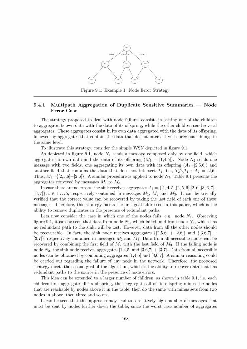
N0

N1 N2 N3

N4 N5

[1,4,5] [2,5,6]+[2,6]

N6 N7

[3,6,7]+[3,7]

Figure 9.1: Example 1: Node Error Strategy

9.4.1 Multipath Aggregation of Duplicate Sensitive Summaries — NodeError Case

The strategy proposed to deal with node failures consists in setting one of the childrento aggregate its own data with the data of its offspring, while the other children send severalaggregates. These aggregates consist in its own data aggregated with the data of its offspring,followed by aggregates that contain the data that do not intersect with previous siblings inthe same level.

To illustrate this strategy, consider the simple WSN depicted in figure 9.1.

As depicted in figure 9.1, node N1 sends a message composed only by one field, whichaggregates its own data and the data of its offspring (M1 = [1,4,5]). Node N2 sends onemessage with two fields, one aggregating its own data with its offspring (A1=[2,5,6]) andanother field that contains the data that does not intersect T1, i.e., T2T1 ; A2 = [2,6].Thus, M2=[2,5,6]+[2,6]. A similar procedure is applied to node N3. Table 9.1 presents theaggregates conveyed by messages M1 to M3.

In case there are no errors, the sink receives aggregates Ai = [1, 4, 5],[2, 5, 6],[2, 6],[3, 6, 7],[3, 7] , i ∈ 1 . . . 5, respectively contained in messages M1, M2 and M3. It can be triviallyverified that the correct value can be recovered by taking the last field of each one of thesemessages. Therefore, this strategy meets the first goal addressed in this paper, which is theability to remove duplicates in the presence of redundant paths.

Lets now consider the case in which one of the nodes fails, e.g., node N1. Observingfigure 9.1, it can be seen that data from node N1, which failed, and from node N4, which hasno redundant path to the sink, will be lost. However, data from all the other nodes shouldbe recoverable. In fact, the sink node receives aggregates [2,5,6] + [2,6] and [3,6,7] +[3,7], respectively contained in messages M2 and M3. Data from all accessible nodes can berecovered by combining the first field of M2 with the last field of M3. If the failing node isnode N2, the sink node receives aggregates [1,4,5] and [3,6,7] + [3,7]. Data from all accessiblenodes can be obtained by combining aggregates [1,4,5] and [3,6,7]. A similar reasoning couldbe carried out regarding the failure of any node in the network. Therefore, the proposedstrategy meets the second goal of the algorithm, which is the ability to recover data that hasredundant paths to the source in the presence of node errors.

This idea can be extended to a larger number of children, as shown in table 9.1, i.e. eachchildren first aggregate all its offspring, then aggregate all of its offspring minus the nodesthat are reachable by nodes above it in the table, then do the same with minus sets from twonodes in above, then three and so on.

It can be seen that this approach may lead to a relatively high number of messages thatmust be sent by nodes further down the table, since the worst case number of aggregates

168

child index message to send

1 T12 T2+ T2\T13 T3+ T3\T1+ T3\T2+ T3\T1 ∪ T2...

...

Table 9.1: Example of aggregates construction for the smallest node numbers in node errorscase.

grows as a power of two. Methods to dramatically reduce the number of entries of such tableare addressed latter on.

Analytical Proof of Reconstruction Capabilities

The last example showed that the node failure case algorithm provides some error correc-tion capabilities. This subsection will establish 1) the basics for the reconstruction algorithmand 2) a formal proof2 that such reconstruction algorithm always achieves its intended goals.The conjunction of 1) and 2) imply that the node failure case algorithm works as advertised.

The algorithm is based on Table 9.1 and it is as follows: whenever data from a givenoffspring is not received, all references from the offspring in question are removed from thetable; the summary is computed as the aggregate of the rightmost elements of the resultingtable.

For the proof of the reconstruction capabilities, note that the resulting table is exactlythe table that would be generated if the node in question only had the offspring that weresuccessfully received. This can be seen by a direct inspection of their structure. Therefore, toprove the point in question, it suffice to prove that in a table such as table 9.1 the aggregateof the rightmost elements of each line equals to the aggregate of the whole table.

The last proposition is proven by induction. In the first case, with only one offspringthe proposition follows by definition. Computing the aggregate recursively, the value of theaggregate at the nth line, is equal to the value of the aggregate of the first n − 1 lines (theinduction) plus the rightmost element of the nth. The rightmost element of the nth line is byconstruction the element that is necessary to be aggregated to the summary of the first n− 1lines in order, concluding the proof.

9.4.2 Multipath Aggregation of Duplicate Sensitive Summaries — LinkError Case

The link error case requires that whenever a link fails, the parent (or the sink) nodereceives all the data necessary to compute all aggregates that are computable, given the linkfailures in question.

The algorithm proposed to achieve this goal consists in having each node sending twoaggregates, one containing the data related to its descendants that are reachable only byitself, and another aggregate composed by the data pertaining to nodes that communicateboth with itself and with its siblings. The algorithm resembles the one presented for thenode error case, except that in the error node case the operation was a bitwise complement,

2that was not written in the form of Theorems due to its rather verbose nature

169

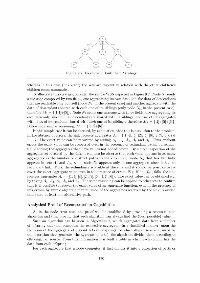
N0

N1 N2 N3

N4 N5

[1,4]+[5] [2]+[5,6]

N6 N7

[3,7]+[6]

Figure 9.2: Example 1: Link Error Strategy

whereas in this case (link error) the sets are disjoint in relation with the other children’schildren count summaries.

To illustrate this strategy, consider the simple WSN depicted in Figure 9.2. Node N1 sendsa message composed by two fields, one aggregating its own data and the data of descendantsthat are reachable only by itself (node N4, in the present case) and another aggregate with thedata of descendants shared with each one of its siblings (only node N5, in the present case),therefore M1 = [1,4]+[5]. Node N2 sends one message with three fields, one aggregating itsown data only, since all its descendants are shared with its siblings, and two other aggregateswith data of descendants shared with each one of its siblings, therefore M2 = [2]+[5]+[6].Following a similar reasoning, M3 = [3,7]+[6].

In this simple case it can be checked, by exhaustion, that this is a solution to the problem.In the absence of errors, the sink receives aggregates Ai = [1, 4], [5], [2], [5], [6], [3, 7], [6], i ∈1 . . . 7. The exact value can be recovered by adding A1, A2, A3, A5 and A6. Thus, withouterrors the exact value can be recovered even in the presence of redundant paths, by sequen-tially adding the aggregates that have values not added before. By simple inspection of theaggregate set received by the sink, it can also be observe that each value appears in as manyaggregates as the number of distinct paths to the sink. E.g. node N5 that has two linksappears in sets A2 and A4, while node N4 appears only in one aggregate, since it has noredundant link. Thus, the redundancy is visible at the sink and it should be possible to re-cover the exact aggregate value even in the presence of errors. E.g. if link L5,1 fails, the sinkreceives aggregates Ai = [1, 4], [ϕ], [2], [5], [6], [3, 7], [6]. The exact value can be obtained e.g.by taking A1, A3, A4, A5 and A6. The same reasoning can be applied to other sets to confirmthat it is possible to recover the exact value of an aggregate function, even in the presence oflink errors, by simple algebraic manipulation of the aggregates received by the sink, providedthat there at least one alternative path.

Analytical Proof of Reconstruction Capabilities

As in the node error case, the proof will be established by providing a reconstructionalgorithm and then proving that such algorithm can always find the (best possible) value.

Such an algorithm can be seen in Algorithm 7, which aggregates data from a numberof offspring and then computes the respective aggregate. In a simplified manner, upon thereception of the aggregate of disjoint sets of offsprings (of which disjointness is ensured bythe algorithm that generates the aggregation lists), the algorithm divides them according tooffspring, i.e. source. From this information it is built a table in which each column has thedata from each offspring.

For each aggregate that a node computes, it first divides it into a collection of parts or

170

sub-aggregates according to the count summary of each offspring. At run time it looks ateach offspring column and if there are entries (sub-aggregates) that a) are necessary for thecomputation of the aggregate and b) are not yet in the list of aggregated entries then it 1) readsthe value in question then 2) add the entry in question to the list of entries (sub-aggregates)that were already aggregated.

For the proof of the correctness of this algorithm its noteworthy that due to the way inwhich the table is built 1) elements in the same row are disjoint and 2) elements of differentrows are either equal or disjoint. Note that given the way in which the data is stored at thereceiver, 1) deals with the intra-node aggregates relationship whereas 2) deals with internodeaggregates relationship. Both points follow directly from an analysis of the aggregate gener-ating algorithm, i.e. Algorithm 5. that are equal because there the use of multipath routingmay introduce duplicates at the receiver.

The proof follows by noting that a) there are no duplications due to the fact that eachsegment is introduced in the aggregate only once and b) whenever there is sufficient datareceived form the offspring to compute the aggregate it will find at least one entry from eachsub-aggregate.

Notwithstanding, there are two aspects that deserve to be pointed out. The first pertainsto the assumption that nodes are fail silent implying that all nodes that do transmit, transmitthe right message. This assumption plus the assumption that all erroneous messages arediscarded imply that all messages with a given sub-aggregate have the same value. Therefore,its value can be retrieved by reading the value of only one such sub-aggregate, which motivatedthe find-and-discard aspect of algorithm 5. Note, however, that if this assumption was not inplace the value of each sub-aggregate could be decided based on some function of the valuesof the various copies.

Another related topic is what is done when there are not enough sub-aggregates to com-pute a particular aggregate. A naıve approach would be to compute the aggregate with theavailable partial sub-aggregates, however, if two or more nodes had to compute the same par-tial aggregate based on different sets of sub-aggregates, they would arrive at different values,implying that the assumption that all nodes that have a copy of a sub-aggregate have the samevalue would no longer be true. Note, however, that this situation is relatively uncommon,but whenever it happens it is impossible to guarantee that the various sub-aggregates will beequal. In fact, it can be seen that among the algorithms that aggregate at that particulardepth, there is none that can guarantee that if there is a path to the sink, then it will becorrectly aggregated.

At this point it is paramount to (formally) introduce the concept of aggregation depth.Aggregation depth is the distance in tree levels from the point of aggregation to the point inwhich the data is generated. For example, it can be said that all node aggregate their owndata with a depth of zero, and their direct parents (if they aggregate) aggregate with a depthof one, and a node grandparent aggregate with a depth of two.

The main issue with link case algorithms is that most of them (the one in this paperincluded) aggregate with relatively small depth, leaving the possibility that the path to thepoint of aggregation may be inaccessible but that there is another path to a higher levelnode that is still accessible, hence not fulfilling their intended goals. Therefore, the only wayof insuring that 1) there will be aggregation, 2) it will be possible to remove duplicates, 3)be resilient to link failures, while still ensuring the best possible aggregation at the sink, isif and only if each data is not aggregated until one level above the first level in which theinformation goes through one and only one node. Let us call the nodes in question first

171

common progenitors of a given data.

Such an optimal approach raises the issue of resource utilization. Since it may mean thata value may cross an entire network without being aggregated (if the node’s first commonprogenitor is the sink). This calls for a compromise between the maximum number of hopesthat a value is allowed to make without being aggregated and the (extra) energy needed totransport such value. At the low energy-near aggregation end is the option of choosing oneparent, send a message only to it and see it aggregated, which essentially is the single pathapproach. At the high energy-high precision end is the option of choosing to aggregate onlyat the first common progenitor.

Note a relationship with the approach in [MYH06], in which the authors used their intu-itions, without any formal analysis proposed a link error type algorithm with an aggregationlevel of at most two.

The link error type explored in this chapter is somewhat in the middle of such scale. Inthis approach two or more values are aggregated at a given level (by all of their parents atsuch level) if and only if all parents of a given sub-aggregate (value) are also parents of allthe other sub-aggregates. Note also that it would be trivial to change the link error casealgorithm as to always aggregate at the first common progenitors.

9.4.3 Aggregate Generation and Data Reconstruction Algorithms

In previous sections, two algorithms to generate aggregates were introduced and illustratedin simple scenarios. Algorithms 4 and 5 describe how the aggregates can be generated forarbitrarily large WSN. In all presented algorithms, #S denotes the cardinality of set S.

Even for the simple cases presented before, it was obvious that a rather high numberof message exchanges would be necessary. In fact, in both cases the worst-case number ofmessages grew as a power of two with the number of siblings. However, it should be notedthat some of the entries of the aggregation tables are empty sets, while others are repeated.The empty sets occurs, for example, if all offspring that a node can reach can also be reachedby at least one of its siblings that are above it in the siblings table. And a repetition mayhappen if, for example, the set of offspring that a node can reach minus the set of nodesfrom a given sibling is equal to a similar set excluding another sibling’s offspring. Therefore,the algorithms herein presented also include an optimization section, in which the generatedaggregate set is pruned of duplicate and empty sets, thus reducing the number and size ofexchanged messages.

Eliminating redundancies (duplicates and empty sets) allows to perform a significant re-duction of messages and aggregates. In sparse networks (logically sparse, not necessarilyphysically sparse) this optimization would not make much difference, since it is likely thateach node would have a rather distinct set of offspring. This is not a problem since underthis circumstances each node would send only one message with the aggregate of its ownvalue and all its children, i.e. sparse networks have less paths in their multipath. However,as the network density grows, there would be more nodes with rather similar offspring tables,thereby the use of this improvement tend to become significant. Nonetheless, it must bestressed that node density control is out of the scope of this chapter.

Algorithm 6 describes how the aggregates can be recovered from the received messagesin the case of node errors. For each aggregate that a node manages (Qk), it must inspectthe aggregates sent by each of its children (Ri). Then, all the entries that failed are removedfrom u. Finally, the correct aggregate value is obtained by taking the rightmost element of

172

Algorithm 4 Node Error Case: Parent Generated Transmission Lists

Ti ← Set of nodes reachable by offspring iP← (Nodes that have been processed)for i = 1; i ≤ number of offsprings; i = i+ 1 do

Mi ← for j = 0; j < i; j = j + 1 do

Z ← Permutation of P taken j by jfor all Zl (elements of Z) do

Mi ← Mi∪

Ti \∪

x∈ZlTx

end forj ← j + 1

end forP← P

∪i

\\Remove duplicates and empty setsfor j = 1; j < 2i−1 − 1; j = j + 1 do

if Mi(j) = thenremove Mi(j)

elsefor k = j + 1; k < 2i−1; k = k + 1 do

if Mi(k) =Mi(j) thenremove Mi(k)

end ifend for

end ifend for

end for

u that has been received from each descendant. As can be verified, the algorithm is notcomputationally intensive. The operations carried out are relatively simple and the numberof iterations depends on the number of aggregates and on the number of children, which arefrequently relatively low values.

Algorithm 7 describes how the aggregates can be recovered from the received messages inthe case of link errors. The process consists in taking the aggregates sent by each childrensequentially, and merge them if they have not been already included from a previous child.To keep track of which values have already been processed, it is used an exclusion list (E). Ineach step this list is appended with the index of all values that have been correctly received(RCi = 1) but not yet merged.

In terms of computational complexity, the algorithm is similar to the previous one.

9.5 Application of the Algorithm

The first aspect of the application of the algorithms proposed herein is that the link errortype of algorithms inherently can cope with node type errors, whereas node type algorithmsare more limited in the link error corrections. The node error correction capabilities of linkerror type algorithms stem from the fact that a node failure is (under the assumption made

173

Algorithm 5 Link Error Case: Parent Generated Transmission Lists

Ti ← Set of nodes reachable by offspring iNi ← number of offspringsfor i = 1; i ≤ N ; i = i+ 1 do

Mi ← Z ← Arrangements of 0, 1 with repetition taken N−1 by N−1for all Zl (elements of Z) do

Mi ← Mi∪

Ti∩

Zl(x)=1 Tx∩

Zl(x)=0 T x

end for

end for\\Remove duplicates and empty setsfor j = 1; j < 2i−1 − 1; j = j + 1 do

if Mi(j) = thenremove Mi(j)

elsefor k = j + 1; k < 2i−1; k = k + 1 do

if Mi(k) =Mi(j) thenremove Mi(k)

end ifend for

end ifend for

herein), in essence, a failure of all of its links.

However, no similar relation can be established between node type algorithms and linkfailures. In fact, whenever there is a link error the assumptions made for the node erroralgorithm no longer hold.

Nevertheless, the node error type algorithms, when applied to networks in which nodefailures are the dominant type of errors, requires less sub-aggregates to be computed (unlessa number of simplification of empty and duplicated sets dictates that it requires the samenumber). Hence, it uses less messages, which in turn is translated into a longer battery life.

With these information at hand it is now possible to make an informed decision aboutthe best algorithm for each approach. Obviously, if there is previous information regardingthe dominant type of error in the network, then it should be chosen a matching algorithm.Otherwise, considerations of energy, computational capacity acceptable error rate shoulddefine the final choice. Similar trade-offs are to be considered when choosing between thealgorithms presented in this article and classical approaches.

9.6 Evaluation

This section presents simulation results to assess the effectiveness of the approaches pro-posed in this paper. The simulations were carried out in the Matlabr software, with astandard error model, in which the error probability is a function of the distance Pr = Ped

−α,with α = 2, transmission power was equal in all the nodes, and the probability of error as(1− erf(Pr/No))/2.

174

Algorithm 6 Node Error Case: Aggregate Computation From Children Messages

Qk ← Set of aggregates that a node managesRi ← Set of aggregate values received from child iRCi ← Binary vector. 1 if received message form child i, 0 otherwiseUk ← Set of reconstruction path to kth aggregateA← \\ Ak ← value of aggregate kfor k = 1; k ≤ #[Qk]; k = k + 1 do

Ak ← selfu← Uk

for i = 1; i ≤ #[Ri]; i = i+ 1 doif not RCi then

for j = i; j ≤ #[Uj ]; j = j + 1 doremove instances of u related to node j

end forend ifAk ← Ak+Ri(argmaxu(i) = 1)

end forend for

In addition to the two algorithms presented in this paper, this section also presents simu-lations of TAG and the DAG approaches, described in Section 9.2. The TAG approach is thesimplest of all. It does not have any type of redundancy, using only simple aggregation, thusit will be used as the base line. The DAG approach has two level deep link error correctioncapability, hence it will be used to perform a comparison with the link error approach pre-sented herein. To the best of the authors knowledge, there is no approach that can be usedto make a direct comparison with the node error case.

The simulation was made with a network with a varying number of nodes, starting from4 nodes, moving upwards with steps of 4, up to 32 nodes. The nodes were placed randomly

Algorithm 7 Link Error Case: Aggregate Computation From Children Messages

Qk ← Set of aggregates that the node handlesRi ← Set of aggregate values received from child iRCi ← Binary vector. 1 if received message form child i, 0 otherwiseUk ← Set of reconstruction path to kth aggregateA← \\ Ak ← value of aggregate kfor k = 1; k ≤ #[Qk]; k = k + 1 do

Ak ← selfE← \\set of excluded aggregatesfor i = 1; i ≤ #[Ri]; i = i+ 1 do

u← Uk \ Uk(RCi = 1)u← u \ EAk ←aggrAk,Ri(u)E← E

∪u

end forend for

175

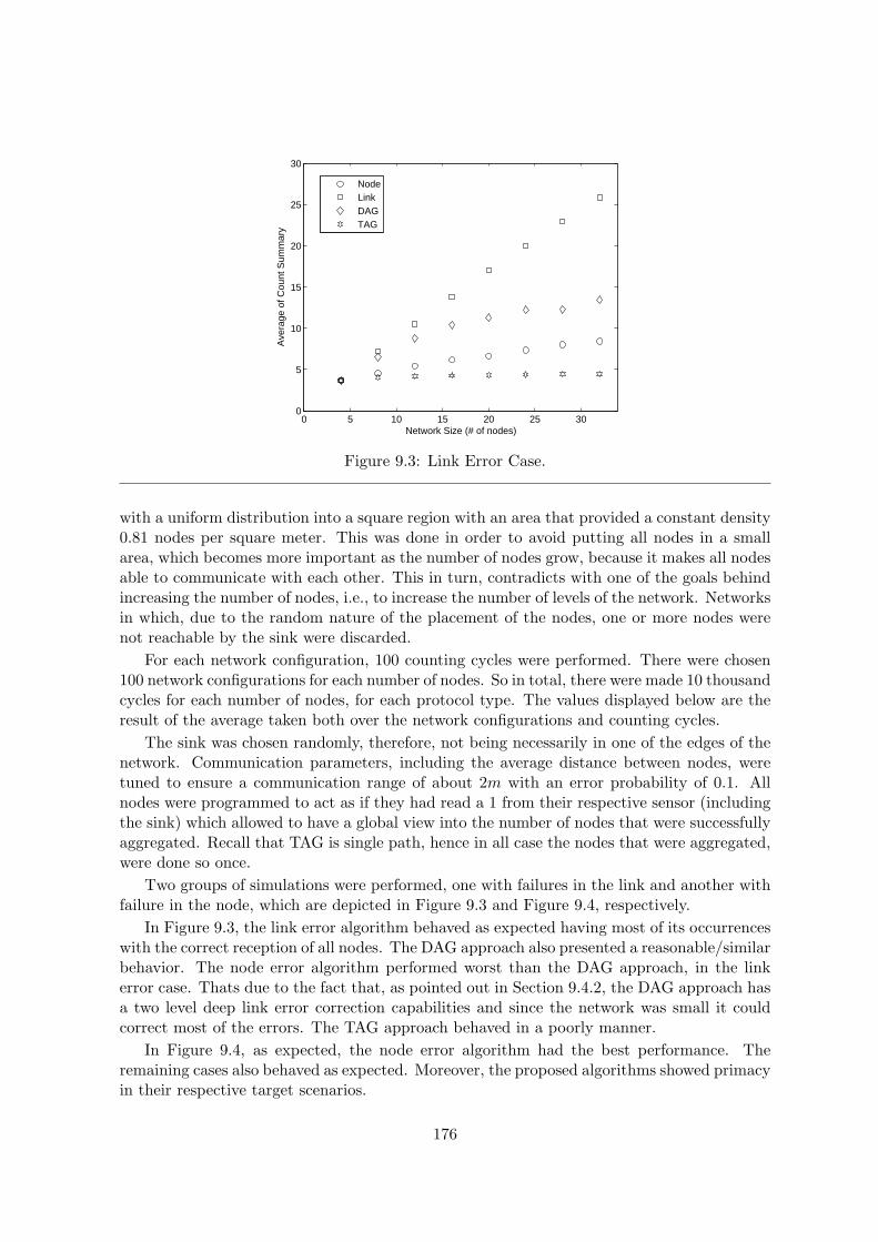
0 5 10 15 20 25 300

5

10

15

20

25

30

Network Size (# of nodes)

Ave

rage

of C

ount

Sum

mar

y

NodeLinkDAGTAG

Figure 9.3: Link Error Case.

with a uniform distribution into a square region with an area that provided a constant density0.81 nodes per square meter. This was done in order to avoid putting all nodes in a smallarea, which becomes more important as the number of nodes grow, because it makes all nodesable to communicate with each other. This in turn, contradicts with one of the goals behindincreasing the number of nodes, i.e., to increase the number of levels of the network. Networksin which, due to the random nature of the placement of the nodes, one or more nodes werenot reachable by the sink were discarded.

For each network configuration, 100 counting cycles were performed. There were chosen100 network configurations for each number of nodes. So in total, there were made 10 thousandcycles for each number of nodes, for each protocol type. The values displayed below are theresult of the average taken both over the network configurations and counting cycles.

The sink was chosen randomly, therefore, not being necessarily in one of the edges of thenetwork. Communication parameters, including the average distance between nodes, weretuned to ensure a communication range of about 2m with an error probability of 0.1. Allnodes were programmed to act as if they had read a 1 from their respective sensor (includingthe sink) which allowed to have a global view into the number of nodes that were successfullyaggregated. Recall that TAG is single path, hence in all case the nodes that were aggregated,were done so once.

Two groups of simulations were performed, one with failures in the link and another withfailure in the node, which are depicted in Figure 9.3 and Figure 9.4, respectively.

In Figure 9.3, the link error algorithm behaved as expected having most of its occurrenceswith the correct reception of all nodes. The DAG approach also presented a reasonable/similarbehavior. The node error algorithm performed worst than the DAG approach, in the linkerror case. Thats due to the fact that, as pointed out in Section 9.4.2, the DAG approach hasa two level deep link error correction capabilities and since the network was small it couldcorrect most of the errors. The TAG approach behaved in a poorly manner.

In Figure 9.4, as expected, the node error algorithm had the best performance. Theremaining cases also behaved as expected. Moreover, the proposed algorithms showed primacyin their respective target scenarios.

176

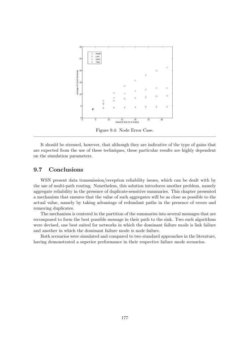
0 5 10 15 20 25 300

5

10

15

20

25

30

Network Size (# of nodes)

Ave

rage

of C

ount

Sum

mar

y

NodeLinkDAGTAG

Figure 9.4: Node Error Case.

It should be stressed, however, that although they are indicative of the type of gains thatare expected from the use of these techniques, these particular results are highly dependenton the simulation parameters.

9.7 Conclusions

WSN present data transmission/reception reliability issues, which can be dealt with bythe use of multi-path routing. Nonetheless, this solution introduces another problem, namelyaggregate reliability in the presence of duplicate-sensitive summaries. This chapter presenteda mechanism that ensures that the value of such aggregates will be as close as possible to theactual value, namely by taking advantage of redundant paths in the presence of errors andremoving duplicates.

The mechanism is centered in the partition of the summaries into several messages that arerecomposed to form the best possible message in their path to the sink. Two such algorithmswere devised, one best suited for networks in which the dominant failure mode is link failureand another in which the dominant failure mode is node failure.

Both scenarios were simulated and compared to two standard approaches in the literature,having demonstrated a superior performance in their respective failure mode scenarios.

177

Chapter 10

Conclusions and Future Lines ofStudy

This work started with the proposal of a novel control architecture for achieving a moreefficient use of network resources. The proposed architecture includes the use of estimatorsand of bulk data transmissions to either attenuate the effects of packet losses or to reducethe overall number of sent packets. Bulk transmissions can be employed at a low or no extrabandwidth cost due to the fact that current fieldbuses have a minimum data length that issignificantly larger than the size of a single control value.

As for the extra computational load incurred for the computation of the estimates, itseffects can be reduced if most of the computing is done at the controller, which usuallyhas more computational resources. This fact, i.e., all heavy lifting done at the controller,limited a number of possibilities of the architecture. The architecture has other advantages,with the most outstanding ones being, 1) the possibility of having the sensor and controllerworking at different rates. This is important, for example, in systems that due to the lowprecision of the available sensors, it is necessary to make a rather large number of samplesto achieve a reasonable estimate, but have a dynamics that do not require a rapid changein actuation value. And 2) this approach already gives more bandwidth to control tasks inwhich the respective controlled processes are in a high error state, a property sought after bythe co-design community.

The architecture was tested in a bandwidth reduction scenario in which the claims madeabout were proven to be true.

The remaining set of characteristics where tested in subsequent developments, namely,when the architecture was used in a scenario with a lossy network. Though, only the controlleractuator side of the architecture was used, it already demonstrated the capabilities that wereargued that the architecture had. Moreover, it was studied the optimal implementation ofsuch scenario.

The study included two possible families of protocols: TCP-like characterized by thepresence of a packet reception acknowledgement and UDP-like characterized by the absenceof such acknowledgment. For both cases, it was devised the optimal noise filtering algorithm,which for the UDP-like case, it was a modified Kalman filter, whereas for the TCP-like caseit was the classical Kalman filter.

As for the controller under this architecture, the certainty equivalence and separationprinciples still hold, implying that the optimal controller is equal to the optimal classical

179

controller. The certainty equivalence and separation principles, in essence, state when thestate estimate can be used with a separately derived controller, can be used in the place ofstate variable, while maintaining the optimality.

Tests of this configuration revealed, as in the previous case, what was expected fromtheoretical considerations. However, this approach still needed a particular underlying archi-tecture. The following case began by looking for controller approaches that were applied tothe general architecture. However, the simplest cases were already solved.

The simplest forms of controller design that are architecture independent is a combinationof TCP-like vs UDP-like and the output zero vs hold. In the output zero scheme, whenevera message is missing, the actuator applies a zero, whereas in the hold approach, whenever,there is a missing message, the actuator maintains the previous value. As for the possiblegeneralizations, the generalizations of TCP-like versus UDP-like into a spectrum, i.e., theprobabilistic reception of acknowledgement messages, is solvable, using modern mathemat-ical tools only for the case in which the acknowledgement is received with probability one,i.e., TCP-like case, because in the remaining cases the certainty equivalence and separationprinciples do not hold.

The logical choice was to extend the zero vs hold case into a situation in which theactuation value, in periods that no control message is received, it was applied a value thatwas equal to the last applied value times a matrix that have no eigenvalue greater than one.Under this approach, and under TCP-like it was derived the optimal control value. Thisproduced a cost function that was itself a function of the matrix used in the actuator tocompute the next control value.

The minimum of the cost function over the actuator transition matrix revealed that suchoptimal implies that the actuator ought to keep an estimate of the controller’s state estimate.Such actuator estimate is updated whenever the actuator receives a controller message andin periods that there are no controller messages it uses a control value computed based on itsstate estimate.

This approach differs significantly from the starting point, which was the architectural ap-proach. Similarities and differences between them were explored, with both having advantagesand disadvantages.

A different line of inquiry was pursued with the goal of permitting the already existingco-design to perform on a more control optimal manner, namely, to ensure that upon theapplication of one of the various techniques to improve the resource optimization that includea controller change, the output does not oscillate. The theoretical work culminated withthe discovery of an algorithm that allowed to perform the controller change without outputoscillation, and it was based on the fact that at the switching instant, the state does notautomatical change in order to represent the new situation.

Most of the computation carried out to implement this strategy is done offline, withthe only online operation being a matrix-vector multiplication. Hence, the algorithm canbe implemented even in systems with relatively low computational capabilities. As for thetask model of the underlying real-time system, it does not need to be changed in order toaccommodate the task responsible to the change of basis. Though, such a new task needsto be executed before the controller in the respective periods in which there is a controllerchange.

The new method was tested against several systems and in all of them it performed asexpected.

Mechanism for introducing and/or tolerating missing jobs (messages) executions (trans-

180

missions) from a real-time perspective were also investigated. In particular, the study had afocus into (m, k)–firm systems. However, it was noted that the existing types of (m, k)–firmsystems are not the best fit to the type of application investigated in this Thesis, becausethe existing systems are either 1) probabilistic, which mean that there is the possibility ofoccurring a relatively long sequence without any controller execution, or 2) its deterministicwith a low utilization.

The (m, k)–firm work done in Thesis was concerned with deterministic (m, k)–firm systemswith a high utilization. It was shown that the approaches that were heralded as being optimalare, in fact, suboptimal. Furthermore, it was presented a mechanism that outperforms allhitherto presented (m, k)–firm schedulers.

The study of transformations of current Wireless Sensor Networks into networks more con-ducive for control purposes was also explored. However, even though contemporary wirelessnetworks possess the relevant characteristics to allow for the use on small control networks,they lack the characteristics that would allow them to deal with wireless networks with alarger number of sensors and actuators. In this Thesis it was proposed a mechanism thatimproves some aspects of wireless networks that are germane for a more precise reading ofmulti-sensor values. The method allows for the joint use of two other strategies that havealready been proposed, i.e., multipath routing and in-network aggregation. However, thesetwo strategies cannot be naively integrated. An evaluation of the proposed scheme showedan improvement over all previous schemes that attempted to achieve similar goals.

10.1 Future Work

Regarding the architecture presented in Chapter 4, there are some benefits of its usethat were not experimentally proven, such as the capacity to online and autonomously givinghigher utilizations to control loops with higher errors, or its use in multi-rate system. Asfor the application of the architecture in lossy scenarios, as presented in Chapter 5, only thecontroller to actuator case was explored. Though, the other case is very similar to the onethat was explored, it could be interesting to know if any new behavior emerges when bothcases are used simultaneously.

As for the optimal generalizations of the output types, it would be very informativeto future engineers to know exactly the computational requirements as well as the type ofperformance gains of each possible version. Moreover, it might also be interesting to explorepossibilities that mix the actuator based compensation, as was done in Chapter 6, withcontroller based compensation, as in Chapter 5.

A similar line can be followed to augment the work presented in Chapter 7, in which thework done can benefit from a validation in a scenario that used an actual co-design mechanism,as opposed to the performed test that consisted in the introduction of signals in the placesthat ideal co-design schedulers would introduce.

In the same integration theme, there is a room for the integration of the (m, k)–firmschedulers presented in Chapter 8, with the control techniques presented in this Thesis. How-ever, some challenges may present themselves since, contrary to the classical deterministic(m, k)–firm schedulers, the presented (dynamic) scheduler (when used online) executes jobsprobabilistically.

As for extensions of the presented work, the possibility of its application under UDP-likeprotocols, which has driven a significant part of the research community, is still an open issue.

181

The work on wireless networks has a rather obvious follow up, namely, its use on itsintended framework, that is, the transport medium of a large distributed control network.

182

Appendix A

Available Fieldbuses

A.1 Controller Area Network

With the growing number of microprocessors present in the average vehicle, Bosch GmbHengineers felt a need in 1983 to come up with a simple protocol that could connect all devices,the Controller Area Network (CAN) protocol [Rob91][Cor08]. Currently, the protocol is onits second version and is used in a wide variety of industrial applications, though the apex ofits use was in the late 90’s and early 2000’s.

CAN is an uncontrolled MAC protocol with a Carrier-Sense Multiple Access (CSMA) non-destructive arbitration scheme. In this MAC there are two signaling bit levels: one recessiveand one dominant. Normally the dominant bit is the logical zero and the recessive is thelogical one, because it simplifies its physical realization, though the norm does not force so.In CAN arbitration, at the beginning of a frame all nodes that are waiting to transmit dataattempt to do so. Whenever a node writes a bit in the bus, it waits a constant amount oftime and then reads it back. If a node writes a recessive bit but reads a dominant bit, then itconsiders to have lost the arbitration and it must stop trying to transmit. However, if a nodewrites a dominant bit and reads a recessive bit, then it considers that there was an error inthe bus and shall start the appropriate response to it.

In order to allow for a larger flexibility, the CAN protocol does not define a physical layer.The bit rates of the CAN bus are specified by the norm and the norm refers to an expectationto see speeds up to 1 Mbps (in part B of the latest specification) [Rob91], or in ISO 11898-2(1Mbps) and ISO 11819-2 (125 Kbps).

In CAN 2.0 there are two frame formats: Standard Format, kept for compatibility reasons,and Extended Format. In the standard format the identifier is 11 bits long while in extendedformat it is 29 bits. This increase allows a wider range of devices to be connected using thesame bus. It also allows a better structuring of the address space since it is used during thearbitration process. However, this address expansion further reduces CAN data efficiency.

In CAN there are several types of frames: Data frames, Remote Frames, Error frames,and overload frames. A data frame comprises seven fields, namely: start of frame, arbitrationfield, control field, data field, CRC field, ACK field, end of frame. Figure A.1 depicts thedata/remote frame format1.

A single dominant bit, called start of frame, is used to end the interframe space which iscomprised only of recessive bits. The format of the arbitration field depends on the version

1image taken from the CAN 2.0 standard.

183

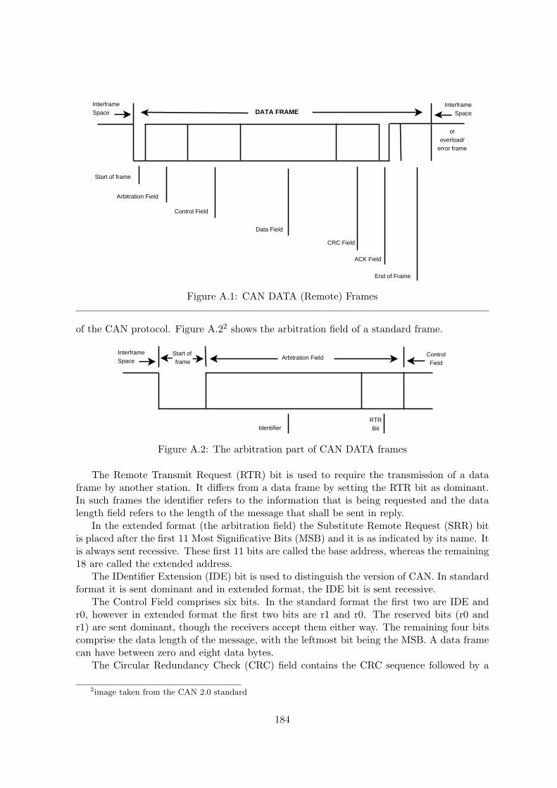
Start of frame

Arbitration Field

Control Field

Data Field

CRC Field

ACK Field

End of Frame

DATA FRAMEInterframeSpace

InterframeSpace

oroverload/

error frame

Figure A.1: CAN DATA (Remote) Frames

of the CAN protocol. Figure A.22 shows the arbitration field of a standard frame.

Start of frame

Arbitration FieldInterframeSpace

ControlField

IdentifierRTRBit

Figure A.2: The arbitration part of CAN DATA frames

The Remote Transmit Request (RTR) bit is used to require the transmission of a dataframe by another station. It differs from a data frame by setting the RTR bit as dominant.In such frames the identifier refers to the information that is being requested and the datalength field refers to the length of the message that shall be sent in reply.

In the extended format (the arbitration field) the Substitute Remote Request (SRR) bitis placed after the first 11 Most Significative Bits (MSB) and it is as indicated by its name. Itis always sent recessive. These first 11 bits are called the base address, whereas the remaining18 are called the extended address.

The IDentifier Extension (IDE) bit is used to distinguish the version of CAN. In standardformat it is sent dominant and in extended format, the IDE bit is sent recessive.

The Control Field comprises six bits. In the standard format the first two are IDE andr0, however in extended format the first two bits are r1 and r0. The reserved bits (r0 andr1) are sent dominant, though the receivers accept them either way. The remaining four bitscomprise the data length of the message, with the leftmost bit being the MSB. A data framecan have between zero and eight data bytes.

The Circular Redundancy Check (CRC) field contains the CRC sequence followed by a

2image taken from the CAN 2.0 standard

184

CRC delimiter, which is a single recessive bit. The CRC is computed using a polynomially, i.e,the CRC is the remaining of the division of the destuffed (more on stuffing in this subsection)version of the fields: Start-Of-Frame (SOF), arbitration, control, data (if present) and for thelowest 15 coefficients by zero.

The Acknowledgement field is two bits long and the first bit is always sent recessive,whereas the second bit is sent dominant if the message is error free and recessive otherwise.A transmission is considered to have been an error if no station receives it correctly.

The CAN protocol also includes an error confinement scheme, which consists of two errorcounters: one for transmission and another for receptions. These counters are initialized withzero and incremented whenever there is an error and decremented whenever a message issuccessfully transmitted/received. When an error counter achieves a given threshold (128) anode becomes error passive, and another threshold (256) it becomes bus off. In the descendingorder it is similar, i.e., at 127 a node passes from error passive to error active. Error active isthe category for fully functional nodes, error passive is for less functional nodes which cannotgenerate error frames, but are able to transmit and receive data frames, and they have lessprivileges. Finally bus off stations cannot use the bus, and future actions of these stationsdepend on an application reset.

An Error Frame contains two fields, error flags and error delimiter, as shown in Figure A.3.Error flags are superpositions of error flags from multiple stations. Error active node signalsthe occurrence of an internal error by sending six consecutive dominant bits, which violatesthe bit stuffing law. Thereby triggering all other error active stations to start transmit theirown error flags. This subfield has between 6 and 12 bits. Error passive stations try to signalerror conditions by waiting for the bus to be free for six consecutive bits. The Error delimiteris a sequence of eight recessive bits.

Error FrameDataFrame

InterframeSpace

Error Flags

Superposition of Error FlagsError Delimiter

orOverload

Frame

Figure A.3: CAN Error Frame

Data Frames and Remote Frames are preceded by an interframe space. The interframespace consists of an intermission field, and a bus idle at the end. The intermission time is 3recessive bits long and the only allowed action during this time is the start of an OverloadFrame. Error passive stations that have been transmitters of the last message must wait anadditional Suspended Transmission time. The suspended transmission time is eight recessivebits long. The bus is said to be idle if after all obligatory interframe space has been fulfilledno station is sending any message.

Overload Frames are sent either if the intermission bits are violated (time between twoframes) or a receiver needs to delay either Data or Remote Frames. Overload frames aresimilar to error frames. Moreover, their fields have similar meanings.

The fields start-of-frame, arbitration, control, data and CRC of the data and remoteframes are encoded using the bit stuff encoding scheme, namely: whenever there are five bits

185

of equally polarity a sixth bit of opposite polarity is inserted with the goal of ensuring that thereceiver of the message is capable of extracting the clock information. The remaining fieldsCRC delimiter, ACK field, and end-of-frame are not encoded in this way. The remainingframes are also not encoded with the bit stuffing scheme. The stuff bits are automaticallyremoved at the receivers.

A.2 Time Triggered CAN (TTCAN)

Though the standard CAN protocol is capable of providing connectivity between multiplenodes, by itself, it does not provide neither jitter nor latency guarantees. Even the highestpriority variable (message) in CAN can be blocked when it gets ready to be sent while an-other message is being sent. To introduce such timing guarantees the TTCAN extension wasintroduced [FMD+00]. TTCAN was standardized as ISO11898-4.

The TTCAN has two levels: level 1 that provides time-triggered operation based on areference message broadcasted by a time master, and fault-tolerance; and a level 2 extension,in which a global time base is guaranteed and a continuous drift correction mechanism isensured.

The most important timing element on TTCAN is the Reference Message. In the level 1extension this message only contains one byte, whereas at level two extension it contains fourbytes used for control, such as the global time information of the current TTCAN master (theconcept of time information is explained in this subsection). The amount of time betweentwo successive reference messages is constant (up to jitter) and defined during network powerup.

The basic cycle is the time that goes from the start of the transmission of a referencemessage to the beginning of the next. Within a basic cycle there are three types of windows,namely: exclusive windows which are used to transmit time-triggered messages, arbitrationwindows which are used to transmit normally arbitrated CAN messages (nodes are not allowedto retry in case of losing the arbitration since this would destroy the basic cycle structure)and free windows. Free windows are used either to allow the expansion of one of the otherwindows types or to allow for the addition of new nodes, given that the scheduling is donestatically.

ExclusiveWindow

FreeWindow

ArbitratingWindow

ExclusiveWindow

ExclusiveWindow

FreeWindow

ArbitratingWindow

ReferenceMessage

ExclusiveWindow

ReferenceMessage

time

Figure A.4: TTCAN Basic Cycle

TTCAN introduces the System Matrix, depicted in Figure A.53, which in essence is agroup of basic cycles that is constantly repeated, in which each basic cycle has its own setof messages. Though the messages vary between two basic cycles in the system matrix, thewindows appear always in the same order and with the same sizes. These windows are calledtransmission columns.

3Image built based on a figure in [FMD+00]

186

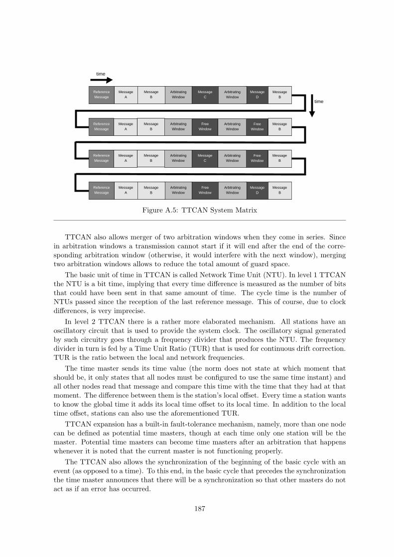
time

MessageA

MessageD

ArbitratingWindow

MessageB

MessageB

MessageC

ArbitratingWindow

ReferenceMessage

MessageA

FreeWindow

ArbitratingWindow

MessageB

MessageB

FreeWindow

ArbitratingWindow

ReferenceMessage

MessageA

FreeWindow

ArbitratingWindow

MessageB

MessageB

MessageC

ArbitratingWindow

ReferenceMessage

MessageA

MessageD

ArbitratingWindow

MessageB

MessageB

FreeWindow

ArbitratingWindow

ReferenceMessage

time

Figure A.5: TTCAN System Matrix

TTCAN also allows merger of two arbitration windows when they come in series. Sincein arbitration windows a transmission cannot start if it will end after the end of the corre-sponding arbitration window (otherwise, it would interfere with the next window), mergingtwo arbitration windows allows to reduce the total amount of guard space.

The basic unit of time in TTCAN is called Network Time Unit (NTU). In level 1 TTCANthe NTU is a bit time, implying that every time difference is measured as the number of bitsthat could have been sent in that same amount of time. The cycle time is the number ofNTUs passed since the reception of the last reference message. This of course, due to clockdifferences, is very imprecise.

In level 2 TTCAN there is a rather more elaborated mechanism. All stations have anoscillatory circuit that is used to provide the system clock. The oscillatory signal generatedby such circuitry goes through a frequency divider that produces the NTU. The frequencydivider in turn is fed by a Time Unit Ratio (TUR) that is used for continuous drift correction.TUR is the ratio between the local and network frequencies.

The time master sends its time value (the norm does not state at which moment thatshould be, it only states that all nodes must be configured to use the same time instant) andall other nodes read that message and compare this time with the time that they had at thatmoment. The difference between them is the station’s local offset. Every time a station wantsto know the global time it adds its local time offset to its local time. In addition to the localtime offset, stations can also use the aforementioned TUR.

TTCAN expansion has a built-in fault-tolerance mechanism, namely, more than one nodecan be defined as potential time masters, though at each time only one station will be themaster. Potential time masters can become time masters after an arbitration that happenswhenever it is noted that the current master is not functioning properly.

The TTCAN also allows the synchronization of the beginning of the basic cycle with anevent (as opposed to a time). To this end, in the basic cycle that precedes the synchronizationthe time master announces that there will be a synchronization so that other masters do notact as if an error has occurred.

187

Synchronous Window (lsw(i))Asynchronous Window (law(i))

Elementary Cycle (EC(i))

TM AM1 SM4 SM8 SM9SM1AM3 AM4 AM8

0 0 0 1 0 0 1 00 1 1

Byte 0Byte 1

bit 1bit 4bit 8bit 9

lsw(i) 1

EC-Schedule

α

Figure A.6: FTT-CAN Elementary Cycle

A.3 Flexible Time Triggered CAN (FTT-CAN)

FTT-CAN [APF22] introduced a distinction between periodic and asynchronous traffic,between time-triggered and event-triggered messages, and between messages with and withouttemporal constraints. FTT-CAN does so by these two types of traffic to coexist in the bus.Therefore, FTT-CAN is a step toward the provisioning of QoS guarantees on the CAN bus.

In FTT-CAN time is divided into fixed duration time-slots called Elementary Cycles (EC).Each EC starts with a Trigger Message (TM), followed by an Asynchronous Window (AW)and a Synchronous Window (SW). The TM is sent in the beginning of the EC. The TM is aconstant size message that contains the duration of the SW and has a bitmap-coded table ofsynchronous messages that will be transmitted in the SW.

The AW is a portion of the EC reserved for asynchronous (event-triggered) traffic. Inthis window the messages are exchanged as in basic CAN, i.e., based in the CAN arbitrationpreviously described. At the end of the AW there is a guarding window in which no stationcan start a transmission, in order to prevent a transmission that would finish after the end ofthe AW. When this window starts retransmissions are also blocked. The duration of the AWis inferred from the duration of the TM and the SW.

At the end of the EC it is the SW. This window is placed at the end of the EC toallow slower nodes to process the TM. In the SW, all nodes with messages scheduled to betransmitted in the current SW, try to transmit their messages simultaneously. The CANMAC ensures that only one message is transmitted at a time. The SW is scheduled centrallyby a master node, which allows to only schedule messages that fit in SW.

Since the FTT-CAN is a high level protocol, it can be decoupled from its physical layer,i.e., CAN, and applied to a different L1/L2 protocol such as Ethernet, as it was done in FTTover shared Ethernet [PGAB05] and FTT over switched Ethernet [Mar09].

A.4 CANopen

CANopen [Cc00] was created for standardizing the higher layer implementations of CANand it is a series of protocols of level three and upper of the OSI model. Due to the fact thatCANopen is a purely higher level protocol it can be implemented in a different lower levelprotocol, being used e.g. in Ethernet POWERLINK and EtherCAT.

CANopen devices logically have three main units: the CAN interface (as pointed outabove, the interface does not need to be CAN), the device’s application, and the interfacebetween the application and the CAN-interface, which is implemented by the Object Dictio-

188

nary. The object dictionary is a list of parameters and provides access to the capabilities ofthe device. The CANopen protocol stack ensures the access to the object dictionary of eachCANopen device. This protocol stack is usually implemented on the same micro-controllerthat is used by the application.

The object dictionary is the main component of CANopen. It is basically a groupingof parameters (or objects in the CANopen terminology) that can be accessed through thenetwork in a pre-defined fashion. Each object in the object dictionary has a 16-bit address(index) and a 8-bit sub-index. The object dictionary is divided in index ranges. A singleCANopen device can have up to eight device/application profile implementations.

CANopen provides a series of bit timing specifications. These include a bit rate, the buslength, maximum stub length and accumulated stub length. Bit rates vary from 10 kbps to 1Mbps. CANopen capable devices are required to support at least one of the bit rates. Otherbit rates are optional.

CANopen provides two mechanisms to verify the functional integrity of nodes: Heartbeatprotocol and the Guarding protocol. In the heartbeat protocol a node periodically broadcastsa message that contains the node’s current NMT (network management) status. A node’sheartbeat protocol transmission period is adjustable. These messages and all other errorrelated messages are sent using an id obtained by adding 700h to the ID of the sending node.

All CANopen devices must support the CANopen Management (MNT) slave state ma-chine. MNT is a state machine that sets the communication behavior of CANopen nodes.MNT can be in one of four states: initialization, pre-operational, operational and stopped.The NMT protocol allows CANopen masters to force state transitions in their slaves. A NMTframe has a sender address of zero (highest CAN priority) ; a future state identifier and aslave identifier. If the identifier field is zero, then all slave must transit to the referred state.

The initialization state contains three other substates, namely initializing, reset applica-tion and reset communication which work as suggested by their names. Whenever a deviceis started or is reset it goes to the initializing state. When a device finishes the initializationof its internal hardware, it goes to the reset application substate.

The boot-up protocol is an error handling protocol that is executed every time a nodetransits from initializing state to pre-operational. In it data fields are set to zero.

Service Data Objects (SDO) provide access to all entries of a CANopen object dictionary,in a confirmed way. It follows a peer-to-peer, client-server model. There are three variantsof the SDO protocol: expedited, normal and block; which work as suggested by their names.SDO message transfers are set up during the initialization of the client device.

There are three types of services specified by the protocol. They are, the synchronization(SYNC), emergency object and time stamp object. Beside SDOs, CANopen provides ProcessData Objects (PDO) that are used to broadcast status and control messages. PDOs requirea set of communication parameters and a set of mapping parameters. These are used, forexample, to state the CAN-id that a PDO will use to communicate, and the type of triggeringevent of the PDO.

There are four types of triggering events: event-(time-)driven, remote request, synchronoustransmission (cyclic) and synchronous transmission (acyclic). Event-(time-)driven triggerhappens whenever an internal state of a device drives it to send a PDO (a sensor reached agiven value or timer went off). A remote request triggered transmission happens whenever aPDO is sent as a response to an RTR. Synchronous (triggered) transmission, both cyclic andacyclic, happen after the transmission of a SYNC message in the bus. The main difference isthat cyclic message are sent in every elementary cycle, while acyclic message are trigger by a

189

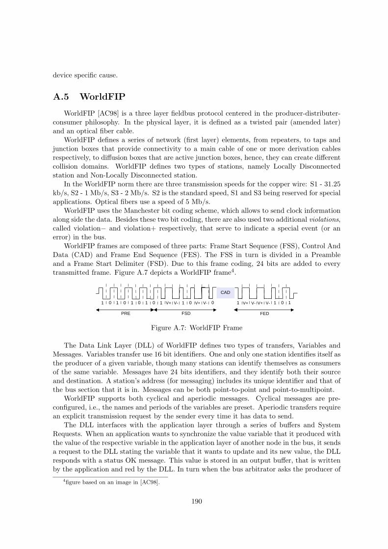
device specific cause.

A.5 WorldFIP

WorldFIP [AC98] is a three layer fieldbus protocol centered in the producer-distributer-consumer philosophy. In the physical layer, it is defined as a twisted pair (amended later)and an optical fiber cable.

WorldFIP defines a series of network (first layer) elements, from repeaters, to taps andjunction boxes that provide connectivity to a main cable of one or more derivation cablesrespectively, to diffusion boxes that are active junction boxes, hence, they can create differentcollision domains. WorldFIP defines two types of stations, namely Locally Disconnectedstation and Non-Locally Disconnected station.

In the WorldFIP norm there are three transmission speeds for the copper wire: S1 - 31.25kb/s, S2 - 1 Mb/s, S3 - 2 Mb/s. S2 is the standard speed, S1 and S3 being reserved for specialapplications. Optical fibers use a speed of 5 Mb/s.

WorldFIP uses the Manchester bit coding scheme, which allows to send clock informationalong side the data. Besides these two bit coding, there are also used two additional violations,called violation− and violation+ respectively, that serve to indicate a special event (or anerror) in the bus.

WorldFIP frames are composed of three parts: Frame Start Sequence (FSS), Control AndData (CAD) and Frame End Sequence (FES). The FSS in turn is divided in a Preambleand a Frame Start Delimiter (FSD). Due to this frame coding, 24 bits are added to everytransmitted frame. Figure A.7 depicts a WorldFIP frame4.

CAD

1 1 1 1 1 1 1 10 0 0 0 0 0 10V+ V+ V+ V+ V-V-V- V-

FEDFSDPRE

Figure A.7: WorldFIP Frame

The Data Link Layer (DLL) of WorldFIP defines two types of transfers, Variables andMessages. Variables transfer use 16 bit identifiers. One and only one station identifies itself asthe producer of a given variable, though many stations can identify themselves as consumersof the same variable. Messages have 24 bits identifiers, and they identify both their sourceand destination. A station’s address (for messaging) includes its unique identifier and that ofthe bus section that it is in. Messages can be both point-to-point and point-to-multipoint.

WorldFIP supports both cyclical and aperiodic messages. Cyclical messages are pre-configured, i.e., the names and periods of the variables are preset. Aperiodic transfers requirean explicit transmission request by the sender every time it has data to send.

The DLL interfaces with the application layer through a series of buffers and SystemRequests. When an application wants to synchronize the value variable that it produced withthe value of the respective variable in the application layer of another node in the bus, it sendsa request to the DLL stating the variable that it wants to update and its new value, the DLLresponds with a status OK message. This value is stored in an output buffer, that is writtenby the application and red by the DLL. In turn when the bus arbitrator asks the producer of

4figure based on an image in [AC98].

190

the variable in question for a new value (if it is a periodically transfer, otherwise the stationwould have to request it), the DLL sends the value that is stored in the corresponding buffer,even if the buffer has not been updated in the last period. After sending the variable to thebus, the DLL sends a signal to the application stating that the variable has been sent.

In case the application layer wants to consume a variable, it indicates so by sending arequest to the DLL in which it states which variable it wants to consume. The DLL answerswith a status OK message. Whenever there is a variable with the same identifier being sentin the bus, the DLL stores in the corresponding buffer and sends a signal to the applicationlayer informing that the variable in question have been received.

The bus traffic generation follows a different philosophy. Whenever the bus arbitratordetects that it is time to poll for a given variable it sends a request frame asking the producerof the referred variable the send the data. The station that identifies itself as being theproducer of the variable sends a response frame with the most recent value of the variable.Symmetrically, the stations that identify themselves as consumers of the variable in question,upon reception of the question frame, prepare to receive the value of the respective variable.

In a WorldFIP bus, only one station can have the function of bus arbitrator, though allstations must be capable of doing so. The bus arbitrator makes a table-based offline staticschedule, and it keeps a table of variables, periods, and data types.

The bus arbitrator takes a different procedure for ensuring the exchange of aperiodicvariables. First the bus arbitrator broadcasts a request frame for a periodic variable A. Ifthe producer of A has any aperiodic variable waiting to be sent then the producer of Abesides responding with the value of A, also requests to send an aperiodic variable. The busarbitrator puts the producer of variable A in queue of producers that have aperiodic trafficto send. There are two such queues, one for urgent transfer and another for normal transfers.

In a window set for aperiodic traffic, in order to isolate the periodic traffic, the busarbitrator asks the producer of variable A for a description of the variables that it wants tosend. Then the producer of A replies with such information, namely: the identifiers of thevariable and their data types; in fact it can reply with up to 64 different variables (assumethat one of this variable is called B). In another windows reserved for aperiodic traffic, (nowthe bus arbitrator uses the same process by which periodic variable are exchanged) the busarbitrator sends a request frame with the identifier of B. The producer of B responds withthe value of B and the consumers of B consume such value.

The producer of a variable is not the only entity capable of starting an aperiodic transferof the variable in question. They can also be started by other entities, such as a consumer ora third-party.

A.6 FlexRay

FlexRay was created by a consortium of automotive companies interested in having afieldbus that matched their exact needs. CAN based fieldbuses had low throughput andEthernet requires a rather complex middleware for providing real-time features. FlexRay wascreated with the purpose of combining the advantages of both. FlexRay is a fieldbus thatdefines all layers of the OSI model, typically involved in a automotive system, allowing it tobe a stand-alone solution to communications.

FlexRay is characterized by a rather high throughput of up to 20 Mbps, if the two channelsare used independently. FlexRay accepts both time and event-triggered traffic. It has a

191

built-in redundancy. It is also fault-tolerant. FlexRay provides mechanisms that improvetransmissions determinism.

In FlexRay terminology the communications controller is referred to as the ElectronicsControl Unit (ECU). Each ECU has a local clock, which must have a precision not worsethan 1.5%, to ensure that any two ECUs have a relative clock drift of less than 3.0%.

During bit transfers, the sender ECU keeps each bit steady for eight cycles. The receiverECU keeps a buffer of the last five bits, and the bit logical value is decided based on a majorityphilosophy.

Each message, called micro-frame in FlexRay, is composed of a Transmission Start Signal(TSS), Frame Start Signal (FSS), data field, Frame End Signal (FES) and Transmission EndSignal (TES). TSS is logical 0, FSS a 1, FES a 0 and TES is logical 1. Bits that compriseeach byte are preceded by two bits: Byte Start Signal 0 and 1 (BSS0 and BSS1) which havethe values 1 and 0 respectively.

Receiving ECUs note an end of transmission by detecting the sequence bit0 - bit1 (FES -TES) after the transmission of a byte, and continue receiving bytes if note the sequence bit1- bit0 (BSS0 - BSS1). Note that each bit correspond to eight cycles.

A bit time is denoted macrotic and is the smallest network time unit. A cycle (of whicha bit is composed of eight) is denoted microtic and is used mostly for bit sampling. Nodessynchronize their clocks to the macrotics.

FlexRay frames are structured in header, payload and trailer. The header is 40 bits longand is comprised by the fields Frame Type, Frame ID, Payload Length, Header CRC. Thepayload field is up to 254 bytes long. The trailer field consists of a 24 bit CRC. Figure A.8illustrates a FlexRay frame.

Frame IDPayloadLength

Header CRCCycleCount

Payload TrailerFrameType

5 bits 11 bits 7 bits 11 bits 6 bits 0 - 254 bytes 3 bytes

Header

Figure A.8: FlexRay Frame

FlexRay has a network cycle with a offline configurable period, which usually is 1 ms.This cycle is divided in four parts: Static Segment, Dynamic Segment, Symbol Window andNetwork Idle Time. The static segment is reserved to offline scheduled Time Division Mul-tiple Access (TDMA) communications. The dynamic segment is reserved for event triggeredcommunications and it is subdivided into macrotics. Nodes with higher priorities are assignedmacrotics closer to the beginning of the dynamic segment. Whenever a node wants to senddata in the dynamic segment it waits until all higher priorities nodes finish sending theirdata. There is a configurable time-out parameter (in number of macrotic) that tells to lowerpriority nodes that if a higher priority node did not start sending data during this time-outis because it will not use the dynamic segment in this period. In case the dynamic segment isfully used by high priority nodes, then lower priority nodes will try again in the next networkcycle.

The symbol window is where all dynamic configurations take place. This window isreserved to the exchange messages used in network maintenance and to signal special networkevents. The Network idle time provides a period of known silence which is used mostly forcycle synchronization.

192

Static WindowDynamicWindow

SymbolWindow

Cycle nCycle n-1 Cycle n+1

Network IdleTime

Figure A.9: FlexRay Cycle

FlexRay also defines a network unit called Central Bus Guardian (CBG). CBGs act inways similar to Ethernet switches, by isolating collision domains or sub-fieldbuses in FlexRayterminology, and all other applications that follow from it. CBG role is mostly policingrelated, providing resilience to errors such as the babbling idiot effect, i.e., when a (failing)node starts sending frames indiscriminately.

FlexRay has a three level error model similar to the CAN error model.

A.7 Time-Triggered Protocol

The Time-Triggered Protocol (TTP) [KG94] was created as a general, physical and MAClayer independent, way of providing real-time guarantees. Thus, it works both in twisted pairand over a optical fiber, without important assumptions. Though TTP has some features thatimprove its performance in situations close to those that appear in the automotive industry.

One of the basis of TTP is that offline TDMA scheduling with distributed clock synchro-nization can be used to reduce the bandwidth used in communications. For example, in TTP,pre-scheduled messages do not require addressing, since all nodes know which message willbe exchange at a particular time. Hence, TTP is a protocol with minimal overhead.

TTP supports different modes, which allows the fieldbus to adequate its behavior to thecurrent application conditions. Each mode is cyclic, with messages repeating themselves, aftera mode dependent amount of time. TTP has mechanisms for providing fast mode switcheswhich are particularly helpful when changing to an emergency mode. Under TTP, modesare characterized by their constituent messages (format, sending node, receiving mode) andrespective schedule/dispatch.

A node is declared to be faulty if in the last TDMA round, no message was sent in the slotreserved for it. A global controller state is maintained. This state contains a list of active andfaulty nodes, in its membership field. Whenever there is a discrepancy in the membershipfield, all nodes participate in a system-wide scrutiny in which for each supposedly fault-node,it is taken the opinion of the majority. Other fields of the controller state are the mode andtime fields.

TTP frames comprise a start-of-frame, control field, data field and CRC. Beside thesethere are interframe spaces. The Control field is 8-bit long, with one initialization bit, threemode change bits and four acknowledgement bits.

By virtue of being time-triggered, TTP has an implicit sending acknowledge. As for thereception acknowledgement, which regards the correctness of the transmitted data, only onenode sends an acknowledgement per message because TTP assumes that situations in whichthe error occurs to a group of nodes and not to others are very rare. TTP also consider thatnodes are fail silent, i.e., faulty nodes are not capable of transmitting messages.

193

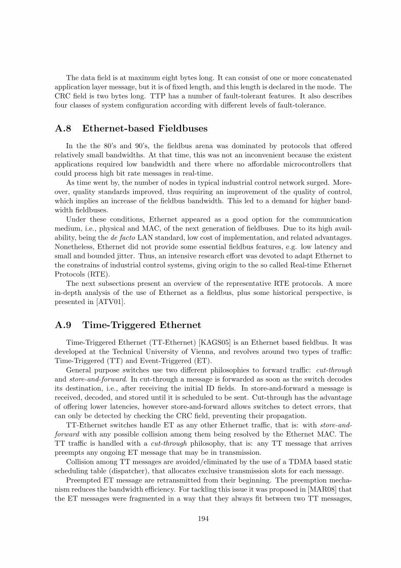
The data field is at maximum eight bytes long. It can consist of one or more concatenatedapplication layer message, but it is of fixed length, and this length is declared in the mode. TheCRC field is two bytes long. TTP has a number of fault-tolerant features. It also describesfour classes of system configuration according with different levels of fault-tolerance.

A.8 Ethernet-based Fieldbuses

In the the 80’s and 90’s, the fieldbus arena was dominated by protocols that offeredrelatively small bandwidths. At that time, this was not an inconvenient because the existentapplications required low bandwidth and there where no affordable microcontrollers thatcould process high bit rate messages in real-time.

As time went by, the number of nodes in typical industrial control network surged. More-over, quality standards improved, thus requiring an improvement of the quality of control,which implies an increase of the fieldbus bandwidth. This led to a demand for higher band-width fieldbuses.

Under these conditions, Ethernet appeared as a good option for the communicationmedium, i.e., physical and MAC, of the next generation of fieldbuses. Due to its high avail-ability, being the de facto LAN standard, low cost of implementation, and related advantages.Nonetheless, Ethernet did not provide some essential fieldbus features, e.g. low latency andsmall and bounded jitter. Thus, an intensive research effort was devoted to adapt Ethernet tothe constrains of industrial control systems, giving origin to the so called Real-time EthernetProtocols (RTE).

The next subsections present an overview of the representative RTE protocols. A morein-depth analysis of the use of Ethernet as a fieldbus, plus some historical perspective, ispresented in [ATV01].

A.9 Time-Triggered Ethernet

Time-Triggered Ethernet (TT-Ethernet) [KAGS05] is an Ethernet based fieldbus. It wasdeveloped at the Technical University of Vienna, and revolves around two types of traffic:Time-Triggered (TT) and Event-Triggered (ET).

General purpose switches use two different philosophies to forward traffic: cut-throughand store-and-forward. In cut-through a message is forwarded as soon as the switch decodesits destination, i.e., after receiving the initial ID fields. In store-and-forward a message isreceived, decoded, and stored until it is scheduled to be sent. Cut-through has the advantageof offering lower latencies, however store-and-forward allows switches to detect errors, thatcan only be detected by checking the CRC field, preventing their propagation.

TT-Ethernet switches handle ET as any other Ethernet traffic, that is: with store-and-forward with any possible collision among them being resolved by the Ethernet MAC. TheTT traffic is handled with a cut-through philosophy, that is: any TT message that arrivespreempts any ongoing ET message that may be in transmission.

Collision among TT messages are avoided/eliminated by the use of a TDMA based staticscheduling table (dispatcher), that allocates exclusive transmission slots for each message.

Preempted ET message are retransmitted from their beginning. The preemption mecha-nism reduces the bandwidth efficiency. For tackling this issue it was proposed in [MAR08] thatthe ET messages were fragmented in a way that they always fit between two TT messages,

194

thus avoiding the retransmission of the initial bytes. The fragmentation/defragmentaion pro-cess is transparent to higher layers.

Beside standard Ethernet components, TT-Ethernet defines a Bus Guardian which is anetwork element, that may be collocated with the TT-Ethernet Switch, be a stand-aloneelement or being instantiated inside a host. The Bus Guardian is used in safety-criticalapplication in order to guarantee a proper functioning of the fieldbus.

TT-Ethernet switches distinguish the TT traffic based on the Ethertype pattern (0x88d7),assigned by the Ethernet standard authority of the IEEE.

Safety Critical TT Ethernet Controller




TTEthernetSwitch

TTEthernetSwitch

Guardian Guardian

HostComputer

HostComputer

HostComputer

HostComputer

Figure A.10: Safety Critical TT-Ethernet Network

TT-Ethernet support various classes of time-triggered traffic, that allows to a differentiatedservice. It also has several types of messages, namely : ET message, Free-Form TT message,TT startup message, TT synchronization message, Unprotected TT message and ProtectedTT message, which work as suggested by their names. Figure A.10 depicts a TT-Ethernetnetwork.

A.10 EtherCAT

Most fieldbuses send many address and control bytes, and relatively a few data bytes.Hence, they have a low data transfer efficiency. This is true even for TT-Ethernet, in whicha small control message is normally encapsulated (with padding) in a long Ethernet frame.

EtherCAT [Groa] was created to solve this issue. It does so by encapsulating severalmessages in a single Ethernet frame. EtherCAT protocol has its own Ethertype. When aEtherCAT node sees the Ethertype in question, it decodes the frame, which consists of variousEtherCAT messages, properly addressed and extract (inserts) the data that is addressed to(produced by) it. EtherCAT nodes decode the message while transmitting them simultane-ously, in a scheme that resembles the cut-through philosophy, thus requiring special-purposeswitches.

This scheme induces an open ring: it starts with the master, which sends a frame withall the requests, goes through the nodes where each node reads either the request for data oran actuation value until the message reaches the end of the ring; in the way back, nodes thatreceived data requests, write down the respective values.

195

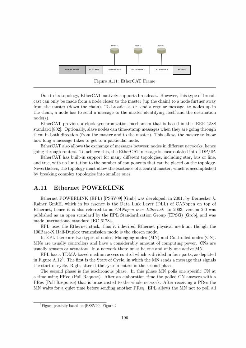
Ethernet Header ECAT HDR DATAGRAM 1 DATAGRAM 2 DATAGRAM 3 Ethernet

Node 1 Node 3Node 2

Figure A.11: EtherCAT Frame

Due to its topology, EtherCAT natively supports broadcast. However, this type of broad-cast can only be made from a node closer to the master (up the chain) to a node further awayfrom the master (down the chain). To broadcast, or send a regular message, to nodes up inthe chain, a node has to send a message to the master identifying itself and the destinationnode(s).

EtherCAT provides a clock synchronization mechanism that is based in the IEEE 1588standard [802]. Optionally, slave nodes can time-stamp messages when they are going throughthem in both direction (from the master and to the master). This allows the master to knowhow long a message takes to get to a particular node.

EtherCAT also allows the exchange of messages between nodes in different networks, hencegoing through routers. To achieve this, the EtherCAT message is encapsulated into UDP/IP.

EtherCAT has built-in support for many different topologies, including star, bus or line,and tree, with no limitation to the number of components that can be placed on the topology.Nevertheless, the topology must allow the existence of a central master, which is accomplishedby breaking complex topologies into smaller ones.

A.11 Ethernet POWERLINK

Ethernet POWERLINK (EPL) [PSSV09] [Gmb] was developed, in 2001, by Bernecker &Rainer GmbH, which in its essence is the Data Link Layer (DLL) of CANopen on top ofEthernet, hence it is also referred to as CANopen over Ethernet. In 2003, version 2.0 waspublished as an open standard by the EPL Standardization Group (EPSG) [Grob], and wasmade international standard IEC 61784.

EPL uses the Ethernet stack, thus it inherited Ethernet physical medium, though the100Base-X Half-Duplex transmission mode is the chosen mode.

In EPL there are two types of nodes, Managing nodes (MN) and Controlled nodes (CN).MNs are usually controllers and have a considerably amount of computing power. CNs areusually sensors or actuators. In a network there must be one and only one active MN.

EPL has a TDMA-based medium access control which is divided in four parts, as depictedin Figure A.125. The first is the Start of Cycle, in which the MN sends a message that signalsthe start of cycle. Right after it the system enters in the second phase.

The second phase is the isochronous phase. In this phase MN polls one specific CN ata time using PReq (Poll Request). After an elaboration time the polled CN answers with aPRes (Poll Response) that is broadcasted to the whole network. After receiving a PRes theMN waits for a quiet time before sending another PReq. EPL allows the MN not to poll all

5Figure partially based on [PSSV09]–Figure 2

196

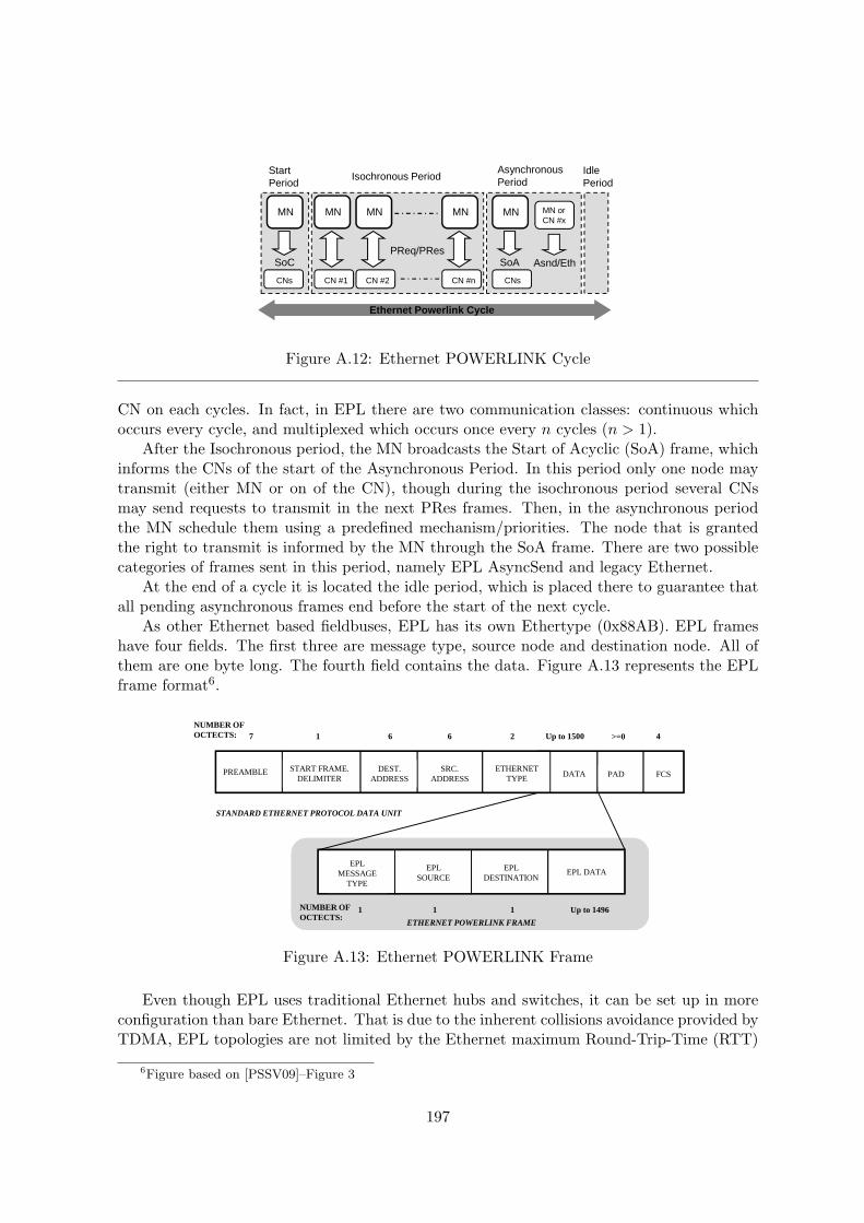
StartPeriod

CN #1

IdlePeriod

AsynchronousPeriodIsochronous Period

MN

SoC

CN #2 CN #n CNs

MN or CN #x

Asnd/Eth

MN MN MN MN

Ethernet Powerlink Cycle

SoAPReq/PRes

CNs

Figure A.12: Ethernet POWERLINK Cycle

CN on each cycles. In fact, in EPL there are two communication classes: continuous whichoccurs every cycle, and multiplexed which occurs once every n cycles (n > 1).

After the Isochronous period, the MN broadcasts the Start of Acyclic (SoA) frame, whichinforms the CNs of the start of the Asynchronous Period. In this period only one node maytransmit (either MN or on of the CN), though during the isochronous period several CNsmay send requests to transmit in the next PRes frames. Then, in the asynchronous periodthe MN schedule them using a predefined mechanism/priorities. The node that is grantedthe right to transmit is informed by the MN through the SoA frame. There are two possiblecategories of frames sent in this period, namely EPL AsyncSend and legacy Ethernet.

At the end of a cycle it is located the idle period, which is placed there to guarantee thatall pending asynchronous frames end before the start of the next cycle.

As other Ethernet based fieldbuses, EPL has its own Ethertype (0x88AB). EPL frameshave four fields. The first three are message type, source node and destination node. All ofthem are one byte long. The fourth field contains the data. Figure A.13 represents the EPLframe format6.

DEST.ADDRESS

SRC.ADDRESS

ETHERNETTYPE DATA FCSPAD

START FRAME.DELIMITER

PREAMBLE

7 1 6 6 2 Up to 1500 >=0 4

STANDARD ETHERNET PROTOCOL DATA UNIT

NUMBER OF OCTECTS:

EPL MESSAGE

TYPE

EPL SOURCE

EPL DESTINATION

EPL DATA

1 1 1 Up to 1496

ETHERNET POWERLINK FRAME

NUMBER OF OCTECTS:

Figure A.13: Ethernet POWERLINK Frame

Even though EPL uses traditional Ethernet hubs and switches, it can be set up in moreconfiguration than bare Ethernet. That is due to the inherent collisions avoidance provided byTDMA, EPL topologies are not limited by the Ethernet maximum Round-Trip-Time (RTT)

6Figure based on [PSSV09]–Figure 3

197

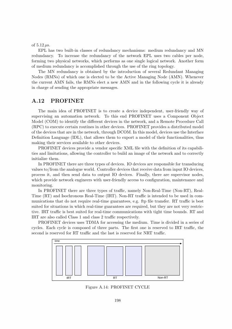
of 5.12µs.

EPL has two built-in classes of redundancy mechanisms: medium redundancy and MNredundancy. To increase the redundancy of the network EPL uses two cables per node,forming two physical networks, which performs as one single logical network. Another formof medium redundancy is accomplished through the use of the ring topology.

The MN redundancy is obtained by the introduction of several Redundant ManagingNodes (RMNs) of which one is elected to be the Active Managing Node (AMN). Wheneverthe current AMN fails, the RMNs elect a new AMN and in the following cycle it is alreadyin charge of sending the appropriate messages.

A.12 PROFINET

The main idea of PROFINET is to create a device independent, user-friendly way ofsupervising an automation network. To this end PROFINET uses a Component ObjectModel (COM) to identify the different devices in the network, and a Remote Procedure Call(RPC) to execute certain routines in other devices. PROFINET provides a distributed modelof the devices that are in the network, through DCOM. In this model, devices use the InterfaceDefinition Language (IDL), that allows them to export a model of their functionalities, thusmaking their services available to other devices.

PROFINET devices provide a vendor specific XML file with the definition of its capabili-ties and limitations, allowing the controller to build an image of the network and to correctlyinitialize them.

In PROFINET there are three types of devices. IO devices are responsible for transducingvalues to/from the analogue world. Controller devices that receive data from input IO devices,process it, and then send data to output IO devices. Finally, there are supervisor nodes,which provide network engineers with user-friendly access to configuration, maintenance andmonitoring.

In PROFINET there are three types of traffic, namely Non-Real-Time (Non-RT), Real-Time (RT) and Isochronous Real-Time (IRT). Non-RT traffic is intended to be used in com-munications that do not require real-time guarantees, e.g. ftp file transfer. RT traffic is bestsuited for situations in which real-time guarantees are required, but they are not very restric-tive. IRT traffic is best suited for real-time communications with tight time bounds. RT andIRT are also called Class 1 and class 2 traffic respectively.

PROFINET devices uses TDMA for accessing the medium. Time is divided in a series ofcycles. Each cycle is composed of three parts. The first one is reserved to IRT traffic, thesecond is reserved for RT traffic and the last is reserved for NRT traffic.

IRT RT Non-RT

time

Figure A.14: PROFINET CYCLE

198

Due to their characteristics each type of traffic has a range of possible/recomended periodsand associated jitters. A typical Non-RT traffic has a period in the range of 100 ms and ajitter as large as its period. RT traffic has a period in the order of 10 ms and jitter up to 15%of the period. IRT can have a periods down to 250 µs, though it normally is in the 1 ms andvirtually no jitter.

There are two variants of the PROFINET protocol: PROFINET CBA (Component BasedAutomation) and PROFINET IO. PROFINET CBA emerged first and introduced many of theconcepts of PROFINET, device abstraction as suggested by the the name. It provides Non-RT and RT (class 1) type of traffic. PROFINET IO, is more focused in real-time applications,and it was introduced due to a demand for motion control, which has tight time constraints.PROFINET IO supports IRT and RT types of traffic.

199

Acronyms

BIBO Bounded-Input Bounded-Output, page 19

C Worst Case Execution Time, page 54

CBS Constant Bandwidth Server, page 63

CPU Central Processing Unit, page 50

CSMA Carrier Sense Multiple Access, page 66

CSMA-CA CSMA Collision Avoidance, page 66

CSMA-CD CSMA Collision Detection, page 66

CSMA-NBA CSMA Non-destructive Bitwise Arbitration, page 66

D Deadline, page 54

DAC Digital-to-Analog Conversion/Converter, page 16

DMS Deadline Monotonic Scheduling, page 58

EDF Earliest Deadline first, page 60

FCFS First Come First Served, page 59

GPC Generalized Predictive Control, page 40

ICSS Integrated Communication and Control Systems, page 50

ISO International Standard Organization, page 63

LLF Least Laxity First, page 61

LQC Linear quadratic control, page 34

LSF Least Slack First, page 61

LTI Linear Time Invariant, page 11

MAC Medium Access Control, page 66

MIMO Multiple-Input Multiple-Output, page 11

mit Minimum Inter-arrival Time, page 54

201

MPC Model Predictive Control, page 40

OSI Open Systems Interconnection, page 63

PCP Priority Ceiling Protocol, page 56

PDC producer-distributor-consumer, page 65

PI Proportional Integrator, page 44

PID Proportional Integral Derivative, page 44

PIP Priority Inheritance Protocol, page 56

QoS Quality of Service, page 49

RMS Rate Monotonic Scheduling, page 56

RMS Root Mean Square, page 20

SISO Single-Input Single-Output, page 11

SOD Send-on-Delta, page 43

T Minimum Inter-arrival Time, page 54

TBS Total Bandwidth Server, page 63

U CPU utilization factor, page 57

WCET Worst Case Execution Time, page 54

202

Bibliography

[802] IEEE 802.3. Carrier sense multiple access with collision detection (csma/cd)access method and physical layer specifications.

[AB98] L. Abeni and G. Buttazzo. Integrating multimedia applications in hard real-time systems. In RTSS ’98: Proceedings of the IEEE Real-Time SystemsSymposium, page 4, Washington, DC, USA, 1998. IEEE Computer Society.

[ABRW91] N.C. Audsley, A. Burns, M. F. Richardson, and A. J. Wellings. Hard real-time scheduling: The deadline-monotonic approach. Proc. IEEE Workshopon Real-Time Operating Systems and Software, pages 133–137, 1991.

[AC98] J.De Azevedo and N. Cravoisy. Worldfip speci-fications. Technical report, Universita di Roma,http://www.dia.uniroma3.it/autom/RetieSistemiAutomazione/PDF/WorldFipProtocol.pdf,1998.

[AKUMK04] J.N. Al-Karaki, R. Ul-Mustafa, and A.E. Kamal. Data aggregation in wirelesssensor networks - exact and approximate algorithms. In High PerformanceSwitching and Routing, 2004. HPSR. 2004 Workshop on, pages 241 – 245,2004.

[AN11] Khaled Ammar and Mario A. Nascimento. On the use of histograms forprocessing exact aggregate queries in wireless sensor networks. InternationalWorkshop on Data Management for Sensor Networks, 8, 2011.

[APF22] Lus Almeida, Paulo Pedreiras, and Jos Alberto Fonseca. The ftt-can protocol:Why and how. IEEE TRANSACTIONS ON INDUSTRIAL ELECTRONICS,49(6):1189–1201, December 22.

[APLW02] L. Abeni, L. Palopoli, G. Lipari, and J. Walpole. Analysis of a reservation-based feedback scheduler. In Real-Time Systems Symposium, 2002. RTSS2002. 23rd IEEE, pages 71–80, 2002.

[APM05] A. Antunes, P. Pedreiras, and A.M. Mota. Adapting the sampling period of areal-time adaptive distributed controller to the bus load. In Emerging Tech-nologies and Factory Automation, 2005. ETFA 2005. 10th IEEE Conferenceon, volume 1, pages 4 pp. –1084, september 2005.

[As03] Babak Azimi-sadjadi. Stability of networked control systems in the presenceof packet losses. In in Proceedings of 2003 IEEE Conference on Decision andControl, pages 676–681, 2003.

203

[AT09] Adolfo Anta and Paulo Tabuada. On the benefits of relaxing the periodicityassumption for networked control systems over can. In Proceedings of the 200930th IEEE Real-Time Systems Symposium, RTSS 09, pages 3–12, Washington,DC, USA, Dec 2009. IEEE Computer Society.

[ATV01] M. Alves, E. Tovar, and F. Vasques. Ethernet goes real-time: a surveyon research and technological developments. Technical report, ISEP-IPP,HURRAY-R-2K01, 2001.

[Bat06] S. Battilotti. Robust detectability from the measurements plus state feedbackstabilization imply semiglobal stabilization from the measurements. AutomaticControl, IEEE Transactions on, 51(9):1542 –1547, sept. 2006.

[BB08] D. Bernardini and A. Bemporad. Energy-aware robust model predictive con-trol based on wireless sensor feedback. In Decision and Control, 2008. CDC2008. 47th IEEE Conference on, pages 3342–3347, 2008.

[BBB03] E. Bini, G.C. Buttazzo, and G.M. Buttazzo. Rate monotonic analysis: the hy-perbolic bound. Computers, IEEE Transactions on, 52(7):933–942, Jul 2003.

[BC01] G. Bernat and R. Cayssials. Guaranteed on-line weakly-hard real-time sys-tems. In Real-Time Systems Symposium, 2001. (RTSS 2001). Proceedings.22nd IEEE, pages 25 – 35, dec. 2001.

[BDSV12] M. Beschi, S. Dormido, J. Sanchez, and A. Visioli. A new two degree-of-freedom event-based pi control strategy. In American Control Conference(ACC), 2012, pages 2362–2367, 2012.

[Ber07] Dimitri P. Bertsekas. Dynamic Programming and Optimal Control, Vol. II.Athena Scientific, 3rd edition, 2007.

[BGPS06] S. Boyd, A. Ghosh, B. Prabhakar, and D. Shah. Randomized gossip algo-rithms. Information Theory, IEEE Transactions on, 52(6):2508 – 2530, june2006.

[BGSS08] M. Ben Gaid, D. Simon, and O. Sename. A convex optimization approachto feedback scheduling. In Control and Automation, 2008 16th MediterraneanConference on, pages 1100–1105, 2008.

[Bla34] H.S. Black. Stabilized feedback amplifiers. Bell Syst. Tech. J., 13:1–18, 1934.

[BLCA02] G.C. Buttazzo, G. Lipari, M. Caccamo, and L. Abeni. Elastic scheduling forflexible workload management. Computers, IEEE Transactions on, 51(3):289–302, mar 2002.

[Bod40] H.W. Bode. Relations between amplitude and phase in feedback amplifierdesign. Bell Syst. Tech. J., 10:421–454, 1940.

[BS72] R. H. Bartels and G. W. Stewart. Solution of the matrix equation ax + xb =c [f4]. Commun. ACM, 15(9):820–826, Sep 1972.

204

[BSJ07] Lei Bao, M. Skoglund, and K.H. Johansson. A scheme for joint quantization,error protection and feedback control over noisy channels. In American ControlConference, 2007. ACC ’07, pages 4905 –4910, july 2007.

[Bur91] A. Burns. Scheduling hard real-time systems: a review. Softw. Eng. J.,6(3):116–128, 1991.

[But97] Giorgio C. Buttazzo. Hard Real-Time Computing: Predictable Scheduling Al-gorithms and Applications. Kluwer Academic Publishers, 1997.

[BV04] Stephen Boyd and Lieven Vandenberghe. Convex Optimization. CambridgeUniversity Press, New York, NY, USA, 2004.

[BVDS11] M. Beschi, A. Visioli, S. Dormido, and J. Sanchez. On the presence of equi-librium points in pi control systems with send-on-delta sampling. In Decisionand Control and European Control Conference (CDC-ECC), 2011 50th IEEEConference on, pages 7843–7848, 2011.

[BVM07] Giorgio Buttazzo, Manel Velasco, and Pau Marti. Quality-of-control manage-ment in overloaded real-time systems. IEEE Trans. Comput., 56:253–266, Feb2007.

[CB08] A. Chaillet and A. Bicchi. Delay compensation in packet-switching networkedcontrolled systems. In Decision and Control, 2008. CDC 2008. 47th IEEEConference on, pages 3620–3625, 2008.

[Cc00] CAN-cia. Canopen protocol. http://www.can-cia.org/index.php?id=84, 3,2000.

[CCC+10] Wei Chen, Ruizhi Chen, Yuwei Chen, H. Kuusniemi, and Jianyu Wang. Aneffective pedestrian dead reckoning algorithm using a unified heading errormodel. In Position Location and Navigation Symposium (PLANS), 2010IEEE/ION, pages 340–347, 2010.

[CCP10] Hyeonjoong Cho, Yongwha Chung, and Daihee Park. Guaranteed dynamicpriority assignment schemes for real-time tasks with (m, k)-firm deadlines.ETRI Journal, 32:422–429, june 2010.

[CE00] A. Cervin and J. Eker. Feedback scheduling of control tasks. In Decision andControl, 2000. Proceedings of the 39th IEEE Conference on, volume 5, pages4871–4876, 2000.

[CEBA02] Anton Cervin, Johan Eker, Bo Bernhardsson, and Karl-Erik Arzen. Feed-backfeedforward scheduling of control tasks. Real-Time Syst., 23:25–53, Jul2002.

[CeSP11] Milton Armando Cunguara, Tomas Antonio Mendes Oliveira e Silva, andPaulo Bacelar Reis Pedreiras. A loosely coupled architecture for networkedcontrol systems. In Industrial Informatics, IEEE 9th International Conferenceon, 2011.

205

[CF03] Martin Corless and Arthur Frazho. Linear Systems and Control — An Oper-ator Perspective. Marcel Dekker, Ink, 2003.

[CF13] G.C. Calafiore and L. Fagiano. Robust model predictive control via scenariooptimization. Automatic Control, IEEE Transactions on, 58(1):219–224, 2013.

[CGKL11] Suan Khai Chong, Mohamed Medhat Gaber, Shonali Krishnaswamy, andSeng Wai Loke. Energy-aware data processing techniques for wireless sen-sor networks: A review. T. Large - Scale Data - and Knowledge-CenteredSystems, 3:117–137, 2011.

[CGMR05] Graham Cormode, Minos Garofalakis, S. Muthukrishnan, and Rajeev Rastogi.Holistic aggregates in a networked world: distributed tracking of approximatequantiles. In Proceedings of the 2005 ACM SIGMOD international conferenceon Management of data, SIGMOD ’05, pages 25–36, New York, NY, USA,2005. ACM.

[Cha03] C.D. Charalambous. Stochastic nonlinear minimax dynamic games with noisymeasurements. Automatic Control, IEEE Transactions on, 48(2):261 – 266,feb. 2003.

[CHH85] Gary B. Lamont Constantine H. Houpis. Digital Control Systems: Theory,Hardware, Software. McGraw-Hill series in electrical engineering. McGraw-Hill, 1985.

[CHL06] Thidapat Chantem, Xiaobo Sharon Hu, and M.D. Lemmon. Generalized elas-tic scheduling. In Real-Time Systems Symposium, 2006. RTSS ’06. 27th IEEEInternational, pages 236–245, dec 2006.

[CLKB04] J. Considine, F. Li, G. Kollios, and J. Byers. Approximate aggregation tech-niques for sensor databases. In Data Engineering, 2004. Proceedings. 20thInternational Conference on, pages 449 – 460, march-2 april 2004.

[CMV08] Silvio Croce, Francesco Marcelloni, and Massimo Vecchio. Reducing powerconsumption in wireless sensor networks using a novel approach to data ag-gregation. Comput. J., 51:227–239, March 2008.

[CMVC06] Rosa Castane, Pau Marti, Manel Velasco, and Anton Cervin. Resource man-agement for control tasks based on the transient dynamics of closed-loop sys-tems. In Proceedings of the 18th Euromicro Conference on Real-Time Systems,pages 171–182, 2006.

[Con10] Online Contributors. Osi model. online: en.wikipedia.org/wiki/OSImodel,2010.

[Cor08] Steve Corrigan. Introduction to the controller area network (can). Applicationreport, Texas Instruments, July 2008.

[CPA+10] T. Cucinotta, L. Palopoli, L. Abeni, D. Faggioli, and G. Lipari. On the inte-gration of application level and resource level qos control for real-time appli-cations. Industrial Informatics, IEEE Transactions on, 6(4):479–491, 2010.

206

[CPX06] Jen-Yeu Chen, G. Pandurangan, and Dongyan Xu. Robust computation of ag-gregates in wireless sensor networks: Distributed randomized algorithms andanalysis. Parallel and Distributed Systems, IEEE Transactions on, 17(9):987–1000, 2006.

[CQG11] Wei Chen, L. Qiu, and Guoxiang Gu. Stabilization of networked multi-inputsystems over awgn channels with channel resource allocation. In Control andAutomation (ICCA), 2011 9th IEEE International Conference on, pages 680–685, 2011.

[CSWS04] Jiming Chen, Yeqiong Song, Zhi Wang, and Youxian Sun. Equivalent matrixdbp for streams with (m,k)-firm deadline. In Industrial Electronics, 2004 IEEEInternational Symposium on, volume 1, pages 675 – 680 vol. 1, may 2004.

[CvdWHN06] M. Cloosterman, N. van de Wouw, M. Heemels, and H. Nijmeijer. Robust sta-bility of networked control systems with time-varying network-induced delays.In Decision and Control, 2006 45th IEEE Conference on, pages 4980–4985,2006.

[CVMC10] Anton Cervin, Manel Velasco, Pau Martı, and Antonio Camacho. Optimal on-line sampling period assignment: Theory and experiments. IEEE Transactionson Control Systems Technology, 19(99):1–9, 2010.

[CZQ12] Wei Chen, Jianying Zheng, and L. Qiu. Linear quadratic optimal control ofcontinuous-time lti systems with random input gains. In Information andAutomation (ICIA), 2012 International Conference on, pages 241–246, 2012.

[Des85] B. Desarthy. Timing constrains of real-time systems: constructs for expressingthem, methods for validating them. IEEE Transactions on Software Engineer-ing, 11(1):80–86, 1985.

[DGM+04] Amol Deshpande, Carlos Guestrin, Samuel R. Madden, Joseph M. Heller-stein, and Wei Hong. Model-driven data acquisition in sensor networks. InProceedings of the Thirtieth international conference on Very large data bases- Volume 30, VLDB ’04, pages 588–599. VLDB Endowment, 2004.

[DKR04] Antonios Deligiannakis, Yannis Kotidis, and Nick Roussopoulos. Hierarchi-cal in-network data aggregation with quality guarantees. In Elisa Bertino,Stavros Christodoulakis, Dimitris Plexousakis, Vassilis Christophides, Mano-lis Koubarakis, Klemens Bhm, and Elena Ferrari, editors, EDBT, volume 2992of Lecture Notes in Computer Science, pages 658–675. Springer, 2004.

[DLG10] Shi-Lu Dai, Hai Lin, and S.S. Ge. Scheduling-and-control codesign for a col-lection of networked control systems with uncertain delays. Control SystemsTechnology, IEEE Transactions on, 18(1):66–78, 2010.

[dM10] Antnio Pereira de Melo. Teoria dos Sistemas de Controlo Lineares. Universi-dade de Aveiro, 2 edition, 2010.

[DSW06] A.G. Dimakis, A.D. Sarwate, and M.J. Wainwright. Geographic gossip: ef-ficient aggregation for sensor networks. In Information Processing in Sensor

207

Networks, 2006. IPSN 2006. The Fifth International Conference on, pages69–76, 2006.

[DVF12] M.L. Della Vedova and T. Facchinetti. Feedback scheduling of real-time phys-ical systems with integrator dynamics. In Emerging Technologies Factory Au-tomation (ETFA), 2012 IEEE 17th Conference on, pages 1–8, 2012.

[EAFR12] M. Elbes, A. Al-Fuqaha, and A. Rayes. Gyroscope drift correction basedon tdoa technology in support of pedestrian dead reckoning. In GlobecomWorkshops (GC Wkshps), 2012 IEEE, pages 314–319, 2012.

[EHA00] Johan Eker, Per Hagander, and Karl-Erik Arzen. A feedback scheduler forreal-time controller tasks. IFAC, Control Engineering Practice, 8:1369–1378,2000.

[ERA07] C. Ebenbauer, T. Raff, and F. Allgower. Certainty-equivalence feedback designwith polynomial-type feedbacks which guarantee iss. Automatic Control, IEEETransactions on, 52(4):716 –720, april 2007.

[ESM07] M. Epstein, Ling Shi, and R.M. Murray. Estimation schemes for networkedcontrol systems using udp-like communication. In Decision and Control, 200746th IEEE Conference on, pages 3945–3951, 2007.

[ESTM08] Michael Epstein, Ling Shi, Abhishek Tiwari, and Richard M. Murray. Prob-abilistic performance of state estimation across a lossy network. Automatica,44(12):3046 – 3053, 2008.

[Eva50] W.R. Evans. Control system synthesis by root locus method. Trans. AIEE,69:1–4, 1950.

[Eve10] C. Evequoz. Guaranteeing optional task completions on (m,k)-firm real-timesystems. In Computer and Information Technology (CIT), 2010 IEEE 10thInternational Conference on, pages 1772–1779, 2010.

[FLS06] K.-W. Fan, S. Liu, and P. Sinha. On the potential of structure-free data aggre-gation in sensor networks. In INFOCOM 2006. 25th IEEE International Con-ference on Computer Communications. Proceedings, pages 1–12, april 2006.

[FMD+00] Thomas Fhrer, Bernd Mller, Werner Dieterle, Florian Hartwich, Robert Hugel,Michael Walther, and Robert Bosch GmbH. Time triggered communicationon can (time triggered can- ttcan). Protocol description, Robert Bosch GmbH,2000.

[FNSLY08] F. Flavia, Jia Ning, F. Simonot-Lion, and Song YeQiong. Optimal on-line(m,k)-firm constraint assignment for real-time control tasks based on plantstate information. In Emerging Technologies and Factory Automation, 2008.ETFA 2008. IEEE International Conference on, pages 908 –915, sept. 2008.

[Foh93] Gerhard Fohler. Realizing Changes of Operational Modes with a Pre Run-TimeScheduled Hard Real-Time System, chapter Dependable computing and faulttolerant system, pages 287–300. Springer Verlag, 1993.

208

[FU95] N.M. Filatov and H. Unbehausen. Adaptive predictive control policy fornonlinear stochastic systems. Automatic Control, IEEE Transactions on,40(11):1943 –1949, nov 1995.

[FU98] N.M. Filatov and H. Unbehauen. Design of improved adaptive controllersusing partial certainty equivalence principle. In American Control Conference.Proceedings of the 1998, volume 2, pages 1068 –1072, jun 1998.

[FV92] Simonot-Lion F. and C. Verlinde. Importance d’un cadre de rfrence dansla mise en place d’une dmarche de dveloppement d’un sustme automis deproduction. Conference Canadienne sur L’automatisation industrielle, 1992.

[GBT+04] Carlos Guestrin, Peter Bodik, Romain Thibaux, Mark Paskin, and SamuelMadden. Distributed regression: an efficient framework for modeling sensornetwork data. In Proceedings of the 3rd international symposium on Infor-mation processing in sensor networks, IPSN ’04, pages 1–10, New York, NY,USA, 2004. ACM.

[GGMH07] Jie Gao, Leonidas Guibas, Nikola Milosavljevic, and John Hershberger. Sparsedata aggregation in sensor networks. In Proceedings of the 6th internationalconference on Information processing in sensor networks, IPSN ’07, pages430–439, New York, NY, USA, 2007. ACM.

[GGP+03] Deepak Ganesan, Ben Greenstein, Denis Perelyubskiy, Deborah Estrin, andJohn Heidemann. An evaluation of multi-resolution storage for sensor net-works. In Proceedings of the 1st international conference on Embedded net-worked sensor systems, SenSys ’03, pages 89–102, New York, NY, USA, 2003.ACM.

[GHBVdW12] T. M P Gommans, W. P M H Heemels, N.W. Bauer, and N. Van de Wouw.Compensation-based control for lossy communication networks. In AmericanControl Conference (ACC), 2012, pages 2854–2859, 2012.

[GJ10] Xiaohua Ge and X. Jiang. A new robust stability criterion of networked controlsystems. In Intelligent Control and Automation (WCICA), 2010 8th WorldCongress on, pages 2855–2860, 2010.

[Gmb] Bernecker & Rainer Industrie-Elektronik GmbH. Powerlink developers page.http://www.br-automation.com.

[GNDC05] Himanshu Gupta, Vishnu Navda, Samir R. Das, and Vishal Chowdhary. Effi-cient gathering of correlated data in sensor networks. In Proceedings of the 6thACM international symposium on Mobile ad hoc networking and computing,MobiHoc ’05, pages 402–413, New York, NY, USA, 2005. ACM.

[GNVL79] G. Golub, S. Nash, and C. Van Loan. A hessenberg-schur method for theproblem ax + xb = c. Automatic Control, IEEE Transactions on, 24(6):909–913, dec 1979.

[Groa] Ethercat Technology Group. Ethercat protocol. Web page.http://www.ethercat.org/en/technology.html.

209

[Grob] Ethernet POWERLINK Standardization Group. Powerlink strandard.http://www.ethernet-powerlink.org.

[GRSK11] P. Goyal, V.J. Ribeiro, H. Saran, and A. Kumar. Strap-down pedestrian dead-reckoning system. In Indoor Positioning and Indoor Navigation (IPIN), 2011International Conference on, pages 1–7, 2011.

[GSC08] E. Garone, B. Sinopoli, and A. Casavola. Lqg control over lossy tcp-like net-works with probabilistic packet acknowledgements. In Decision and Control,2008. CDC 2008. 47th IEEE Conference on, pages 2686–2691, 2008.

[GSGC12] E. Garone, B. Sinopoli, A. Goldsmith, and A. Casavola. Lqg control formimo systems over multiple erasure channels with perfect acknowledgment.Automatic Control, IEEE Transactions on, 57(2):450–456, 2012.

[GSHM05] Vijay Gupta, Demetri Spanos, Babak Hassibi, and Richard M Murray. Opti-mal lqg control across packet-dropping links. In Systems and Control Letters,pages 360–365. Accepted, 2005.

[HA88] Yoram Halevi and Ray Asok. Integrated communication and control system:Part i—analysis. Journal of Dynamic Systems, Measurement, and Control,110:367–373, Dec 1988.

[Haz34] H.L. Hazen. Theory of servomechanisms. J. Franklin Inst, 218:283–331, 1934.

[HBG10] A. Hakiri, P. Berthou, and T. Gayraud. Qos-enabled anfis dead reckoningalgorithm for distributed interactive simulation. In Distributed Simulationand Real Time Applications (DS-RT), 2010 IEEE/ACM 14th InternationalSymposium on, pages 33–42, 2010.

[HC05] D. Henriksson and A. Cervin. Optimal on-line sampling period assignmentfor real-time control tasks based on plant state information. In Decision andControl, 2005 and 2005 European Control Conference. CDC-ECC ’05. 44thIEEE Conference on, pages 4469–4474, 2005.

[HCB00] Wendi Rabiner Heinzelman, Anantha Chandrakasan, and Hari Balakrishnan.Energy-efficient communication protocol for wireless microsensor networks. InProceedings of the 33rd Hawaii International Conference on System Sciences-Volume 8, volume 8 of HICSS ’00, pages 8020–, Washington, DC, USA, 2000.IEEE Computer Society.

[HGT99] J. Hildebrandt, F. Golatowski, and D. Timmermann. Scheduling coprocessorfor enhanced least-laxity-first scheduling in hard real-time systems. In Pro-ceedings of the 11th Euromicro Conference on Real-Time Systems, volume 11,pages 208 –215, 1999.

[HHLH10] R.C. Harvey, A. Hamza, Cong Ly, and M. Hefeeda. Energy-efficient gamingon mobile devices using dead reckoning-based power management. In Networkand Systems Support for Games (NetGames), 2010 9th Annual Workshop on,pages 1–6, 2010.

210

[HLC12] M. Heidarinejad, Jinfeng Liu, and P.D. Christofides. Distributed model pre-dictive control of switched nonlinear systems. In American Control Conference(ACC), 2012, pages 3198–3203, 2012.

[HNX07] Joao P. Hespanha, Payam Naghshtabrizi, and Yonggang Xu. A survey ofrecent results in networked control systems. In Proceedings of the IEEE, pages138–162, 2007.

[HOV02] Joo Hespanha, Antonio Ortega, and Lavanya Vasudevan. Towards the controlof linear systems with minimum bit-rate. In In Proc. of the Int. Symp. on theMathematical Theory of Networks and Syst, 2002.

[HR95] M. Hamdaoui and P. Ramanathan. A dynamic priority assignment techniquefor streams with (m, k)–firm deadlines. Computers, IEEE Transactions on,44(12):1443 –1451, dec 1995.

[HRS07] Christiaan Heij, Andr Ran, and Freek van Schagen. Introduction to Mathe-matical Systems Theory. Birkhauser Basel, 2007.

[HS05] Lars Peter Hansen and Thomas J. Sargent. Certainty equivalence and modeluncertainty. Proceedings, Board of Governors of the Federal Reserve System(U.S.), pages 17–38, 2005.

[HSJ08] E. Henriksson, H. Sandberg, and K.H. Johansson. Predictive compensationfor communication outages in networked control systems. In Decision andControl, 2008. CDC 2008. 47th IEEE Conference on, pages 2063–2068, 2008.

[HV01] D. Hristu-Varsakelis. Feedback control systems as users of a shared network:communication sequences that guarantee stability. In Decision and Control,2001. Proceedings of the 40th IEEE Conference on, volume 4, pages 3631–3636,2001.

[HY07] Shawn Hu and Wei-Yong Yan. Stability robustness of networked control sys-tems with respect to packet loss. Automatica, 43(7):1243–1248, 2007.

[HY08] Shawn Hu and Wei-Yong Yan. Stability of networked control systems undera multiple-packet transmission policy. Automatic Control, IEEE Transactionson, 53(7):1706 –1711, aug. 2008.

[Int87] Interbusclub, www.interbusclub.com/en/doku/pdf/interbusbasicsen.pdf. In-terbus Protocol, 1987.

[IYB06] Orhan C. Imer, Serdar Yuksel, and Tamer Basar. Optimal control of lti sys-tems over unreliable communication links. Automatica, 42:1429–1439, Septem-ber 2006.

[JJ07] Sirkka-Liisa Jamsa-Jounela. Future trends in process automation. AnnualReviews in Control, 31(2):211 – 220, 2007.

[JP86] M. Joseph and P. Pandya. Finding Response Times in a Real-Time System.The Computer Journal, 29(5):390–395, 1986.

211

[JP04] A. Jindal and K. Psounis. Modeling spatially-correlated sensor network data.In Sensor and Ad Hoc Communications and Networks, 2004. IEEE SECON2004. 2004 First Annual IEEE Communications Society Conference on, pages162 – 171, oct. 2004.

[JW08] Sherif Abdelwahed Jian Wu. An efficient finite-input receding horizon controlmethod and its application for the pneumatic hopping robot. JOURNAL OFCOMPUTERS, 3(9):50–57, September 2008.

[JYQ06] Li Jian and Song Ye-Qiong. Relaxed (m, k)-firm constraint to improve real-time streams admission rate under non pre-emptive fixed priority scheduling.In Emerging Technologies and Factory Automation, 2006. ETFA ’06. IEEEConference on, pages 1051 –1060, sept. 2006.

[KAGS05] H. Kopetz, A. Ademaj, P. Grillinger, and K. Steinhammer. The time-triggeredethernet (tte) design. In Object-Oriented Real-Time Distributed Computing,2005. ISORC 2005. Eighth IEEE International Symposium on, pages 22–33,May 2005.

[KBAF11] Markus J. Koegel, Rainer Blind, Frank Allgower, and Rolf Findeisen. Optimaland optimal-linear control over lossy, distributed networks. Proceedings of the18th IFAC World Congress, 18:13239–13244, 2011.

[KC11] Yeonhwa Kong and Hyeonjoong Cho. Guaranteed scheduling for (m,k)-firmdeadline-constrained real-time tasks on multiprocessors. In Parallel and Dis-tributed Computing, Applications and Technologies (PDCAT), 2011 12th In-ternational Conference on, pages 18–23, 2011.

[KDG03] D. Kempe, A. Dobra, and J. Gehrke. Gossip-based computation of aggregateinformation. In Foundations of Computer Science, 2003. Proceedings. 44thAnnual IEEE Symposium on, pages 482 – 491, oct. 2003.

[KDN02] Konstantinos Kalpakis, Koustuv Dasgupta, and Parag Namjoshi. Maximumlifetime data gathering and aggregation in wireless sensor networks. Proceed-ings of IEEE Networks, 2002.

[KEW02] Bhaskar Krishnamachari, Deborah Estrin, and Stephen B. Wicker. The impactof data aggregation in wireless sensor networks. In Proceedings of the 22ndInternational Conference on Distributed Computing Systems, ICDCSW ’02,pages 575–578, Washington, DC, USA, 2002. IEEE Computer Society.

[KF11] Markus Kogel and R. Findeisen. Robust suboptimal control over lossy net-works using extended input schemes. In Computer-Aided Control System De-sign (CACSD), 2011 IEEE International Symposium on, pages 210–215, 2011.

[KG94] Hermann Kopetz and Gunter Grunsteidl. Ttp-a protocol for fault-tolerantreal-time systems. Computer, 27(1):14–23, 1994.

[Kim10] Ki-Il Kim. A novel scheduling for (m, k)-firm streams in wireless sensornetworks. In Networked Computing and Advanced Information Management(NCM), 2010 Sixth International Conference on, pages 553 –556, aug. 2010.

212

[Kired] Donald E. Kirk. Optimal Control Theory: An Introduction. Dover Books onElectrical Engineering, 2004 (republished).

[KJA97] Bjorn Wittenmark Karl J. Astrom. Computer Controlled Systems: Theoryand Design. Prentice Hall, 3 edition, 1997.

[KKH04] Kyong Hoon Kim, Jong Kim, and Sung Je Hong. Best-effort scheduling (m,k)-firm real-time tasks based on the (m, k)-firm constraint meeting probability.In ESA/VLSI’04, pages 240–248, 2004.

[KKH+08] Xenofon Koutsoukos, Nicholas Kottenstette, Joe Hall, Panos Antsaklis, andJanos Sztipanovits. Passivity-based control design of cyberphysical systems.In In International Workshop on CyberPhysical Systems - Challenges and Ap-plications (CPSCA08, 2008.

[KM11] M.R. Kandroodi and B. Moshiri. Identification and model predictive control ofcontinuous stirred tank reactor based on artificial neural networks. In Control,Instrumentation and Automation (ICCIA), 2011 2nd International Conferenceon, pages 338–343, 2011.

[Kop91] H. Kopetz. Operating Systems of the 90s and Beyond, volume 563 of LectureNotes in Computer Science (LNCS), chapter Event-Triggered versus Time-Triggered Real-Time Systems, pages 86–101. Springer Berlin / Heidelberg,1991.

[Kop97] Hermann Kopetz. Real-Time Systems: Design Principles for Distributed Em-bedded Applications, volume 395 of The Springer International Series in En-gineering and Computer Science. Springer, April 1997.

[Kr99] Andrzej Krlikowski. Adaptive generalized predictive control subject to inputconstraints. In Proceedings of the 7th Mediterranean Conference on Controland Automation (MED99) Haifa, Israel, volume 7. IEEE, IEEE, june 1999.

[KS95] G. Koren and D. Shasha. Skip-over: algorithms and complexity for overloadedsystems that allow skips. In Real-Time Systems Symposium, 1995. Proceed-ings., 16th IEEE, pages 110–117, 1995.

[LB02] B. Lincoln and B. Bernhardsson. Lqr optimization of linear system switching.Automatic Control, IEEE Transactions on, 47(10):1701–1705, 2002.

[LC06] J. Lin and A.M.K. Cheng. Maximizing guaranteed qos in (m, k)-firm real-timesystems. In Embedded and Real-Time Computing Systems and Applications,2006. Proceedings. 12th IEEE International Conference on, pages 402 –410,0-0 2006.

[Leh90] J.P. Lehoczky. Fixed priority scheduling of periodic task sets with arbitrarydeadlines. In Real-Time Systems Symposium, Proceedings., volume 11, pages201–209, Dec 1990.

[Lev96] William Levine, editor. The Control Handbook. CRC Press and IEEE Press,1996.

213

[LG96] Marco Spuri Laurent George, Nicolas Rivierre. Preempive and non-preemptivereal-time uni-processor scheduling. Research report 2772, Institut National deRecherche, Sep 1996.

[Lin07] Mikael Lindberg. A Survey of Reservation-Based Scheduling. Department ofAutomatic Control, Lund Institute of Technology, October 2007.

[LK12] BiJun Li and Ki-Il Kim. A novel routing protocol for (m, k)-firm-based real-time streams in wireless sensor networks. In Wireless Communications andNetworking Conference (WCNC), 2012 IEEE, pages 1715–1719, 2012.

[LKF07] Wen-Hwa Liao, Yucheng Kao, and Chien-Ming Fan. An ant colony algorithmfor data aggregation in wireless sensor networks. In Proceedings of the 2007International Conference on Sensor Technologies and Applications, SENSOR-COMM ’07, pages 101–106, Washington, DC, USA, 2007. IEEE ComputerSociety.

[LL73] Liu and Layland. Scheduling algorithms for multi-programming in a hard-realtime. Journal of the Association for Computing Machinery, 20(1), January1973.

[LL12] Chi-Ying Lin and Yen-Chung Liu. Precision tracking control and constrainthandling of mechatronic servo systems using model predictive control. Mecha-tronics, IEEE/ASME Transactions on, 17(4):593–605, 2012.

[LMV10] C. Lozoya, P. Marti, and M. Velasco. Minimizing control cost in resource-constrained control systems: From feedback scheduling to event-driven control.In Control Automation (MED), 2010 18th Mediterranean Conference on, pages267–272, 2010.

[LMVF08a] C. Lozoya, P. Marti, M. Velasco, and J.M. Fuertes. Analysis and design ofnetworked control loops with synchronization at the actuation instants. InIndustrial Electronics, 2008. IECON 2008. 34th Annual Conference of IEEE,volume 34, pages 2899–2904, November 2008.

[LMVF08b] Camilo Lozoya, Pau Martı, Manel Velasco, and Josep M. Fuertes. Controlperformance evaluation of selected methods of feedback scheduling of real-time control tasks. In 17th IFAC World Congress, July 2008.

[LSF+03] Bruno Sinopoli Luca, Luca Schenato, Massimo Franceschetti, KameshwarPoolla, Michael I. Jordan, and Shankar S. Sastry. Kalman filtering with in-termittent observations. IEEE Transactions on Automatic Control, 49:1453–1464, 2003.

[LSSL06] J. Li, Y. Song, and F. Simonot-Lion. Providing real-time applications withgraceful degradation of qos and fault tolerance according to -firm model. In-dustrial Informatics, IEEE Transactions on, 2(2):112–119, may 2006.

[LSST02] Chenyang Lu, John A. Stankovic, Sang H. Son, and Gang Tao. Feedbackcontrol real-time scheduling: Framework, modeling, and algorithms*. Real-Time Syst., 23(1/2):85–126, July 2002.

214

[LW82] J. Y. T. Leung and J. Whitehead. On the complexity of fixed-priority schedul-ing of periodic, real-time tasks. Performance Evaluation, 2:237–250, 1982.

[LW12] Bing Li and Junfeng Wu. A new delay-dependent stability criteria for net-worked control systems. Journal of Theoretical and Applied Information Tech-nology, 43(1):127–133, Sep 2012.

[LY08] Li Lanying and Tan Yu. Analysis and improvement of scheduling algorithmsbased on (m, k)-firm constraint. In Computer Science and ComputationalTechnology, 2008. ISCSCT ’08. International Symposium on, volume 2, pages74 –77, dec. 2008.

[LZ10] Tao Li and Ji-Feng Zhang. Decentralized adaptive games for large populationcoupled arx systems with unknown coupling strength. In Decision and Control(CDC), 2010 49th IEEE Conference on, pages 3110 –3115, dec 2010.

[LZFA05] Hai Lin, Guisheng Zhai, Lei Fang, and Panos Antsaklis. Stability and h∞performance preserving scheduling policy for networked control systems. Pro-ceedings of the 16th IFAC World Congress, 16:435–400, 2005.

[MA01] A. Manjeshwar and D.P. Agrawal. Teen: a routing protocol for enhancedefficiency in wireless sensor networks. In Parallel and Distributed ProcessingSymposium., Proceedings 15th International, pages 2009 –2015, apr 2001.

[MA02] Arati Manjeshwar and Dharma P. Agrawal. Apteen: A hybrid protocol forefficient routing and comprehensive information retrieval in wireless sensornetworks. In Proceedings of the 16th International Parallel and DistributedProcessing Symposium, IPDPS ’02, pages 48–55, Washington, DC, USA, 2002.IEEE Computer Society.

[MAR08] V. Mikolasek, A. Ademaj, and S. Racek. Segmentation of standard ether-net messages in the time-triggered ethernet. In Emerging Technologies andFactory Automation, 2008. ETFA 2008. IEEE International Conference on,pages 392–399, Sept. 2008.

[Mar09] Ricardo Marau. Real-time communications over switched Ethernet supportingdynamic QoS management. PhD thesis, Universidade de Aveiro Departamentode Electrnica, Telecomunicaes e Informtica, December 2009.

[MAX68] J.C. MAXWELL. On governors. In Proceedings of the Royal Society, number100, 1868.

[MCH10] Zhongjing Ma, D. Callaway, and I. Hiskens. Decentralized charging control forlarge populations of plug-in electric vehicles: Application of the nash certaintyequivalence principle. In Control Applications (CCA), 2010 IEEE Interna-tional Conference on, pages 191 –195, sept. 2010.

[MFFR02] P. Marti, J.M. Fuertes, G. Fohler, and K. Ramamritham. Improving quality-of-control using flexible timing constraints: metric and scheduling. In Real-TimeSystems Symposium, 2002. RTSS 2002. 23rd IEEE, pages 91–100, 2002.

215

[MFHH02] Samuel Madden, Michael J. Franklin, Joseph M. Hellerstein, and Wei Hong.Tag: a tiny aggregation service for ad-hoc sensor networks. SIGOPS Oper.Syst. Rev., 36:131–146, December 2002.

[MH09] A. Molin and S. Hirche. On lqg joint optimal scheduling and control undercommunication constraints. In Decision and Control, 2009. CDC/CCC 2009.Proceedings of the 48th IEEE Conference on, pages 5832 –5838, dec. 2009.

[MLV+08] R. Marau, P. Leite, M. Velasco, P. Marti, L. Almeida, P. Pedreiras, and J.M.Fuertes. Performing flexible control on low-cost microcontrollers using a min-imal real-time kernel. Industrial Informatics, IEEE Transactions on, 4(2):125–133, May 2008.

[MNG05] Amit Manjhi, Suman Nath, and Phillip B. Gibbons. Tributaries and deltas:efficient and robust aggregation in sensor network streams. In Proceedings ofthe 2005 ACM SIGMOD international conference on Management of data,SIGMOD ’05, pages 287–298, New York, NY, USA, 2005. ACM.

[MQF12] R. Muradore, D. Quaglia, and P. Fiorini. Predictive control of networked con-trol systems over differentiated services lossy networks. In Design, AutomationTest in Europe Conference Exhibition (DATE), 2012, pages 1245–1250, 2012.

[MSSG12] Yilin Mo, B. Sinopoli, Ling Shi, and E. Garone. Infinite-horizon sensor schedul-ing for estimation over lossy networks. In Decision and Control (CDC), 2012IEEE 51st Annual Conference on, pages 3317–3322, 2012.

[MSZ11] R. Majumdar, I. Saha, and Majid Zamani. Performance-aware scheduler syn-thesis for control systems. In Embedded Software (EMSOFT), 2011 Proceed-ings of the International Conference on, pages 299–308, 2011.

[MVB09] Pau Martı, Manel Velasco, and Enrico Bini. The optimal boundary and regu-lator design problem for event-driven controllers. In Proceedings of the 12th In-ternational Conference on Hybrid Systems: Computation and Control, HSCC’09, pages 441–444, 2009.

[MWW12] S.C. McLoone, P.J. Walsh, and T.E. Ward. An enhanced dead reckoning modelfor physics-aware multiplayer computer games. In Distributed Simulation andReal Time Applications (DS-RT), 2012 IEEE/ACM 16th International Sym-posium on, pages 111–117, 2012.

[MYH06] S. Motegi, K. Yoshihara, and H. Horiuchi. Dag based in-network aggregationfor sensor network monitoring. In Applications and the Internet, 2006. SAINT2006. International Symposium on, pages 8 pp. –299, jan. 2006.

[MZ95] N. Malcom and W. Zhao. Hard real-time communication in multiple-accessnetworks. In Kluwer Academic Publishers, editor, Real Time Systems, vol-ume 9, pages 75–107, Boston, USA, 1995.

[NFZE07] G.N. Nair, F. Fagnani, S. Zampieri, and R.J. Evans. Feedback control underdata rate constraints: An overview. Proceedings of the IEEE, 95(1):108 –137,Jan 2007.

216

[NGSA04] Suman Nath, Phillip B. Gibbons, Srinivasan Seshan, and Zachary R. Ander-son. Synopsis diffusion for robust aggregation in sensor networks. In Pro-ceedings of the 2nd international conference on Embedded networked sensorsystems, SenSys ’04, pages 250–262, New York, NY, USA, 2004. ACM.

[NP04] Eduardo Tovar Nuno Pereira, Luis Miguel Pinho. Ethernet-based systems:Contributions to the holistic analysis. Proceedings of the 16th Euromicro Con-ference on Real-time Systems (ECRTS’4), 4:25–28, july 2004.

[NQ06] Linwei Niu and Gang Quan. Energy minimization for real-time systems with(m,k)-guarantee. Very Large Scale Integration (VLSI) Systems, IEEE Trans-actions on, 14(7):717–729, 2006.

[NS07] Vinh Hao Nguyen and Young Soo Suh. Improving estimation performance innetworked control systems applying the send-on-delta transmission method.Sensors 2007, 7(10):2128–2138, October 2007.

[NS08] Vinh Hao Nguyen and Young Soo Suh. Networked estimation with an area-triggered transmission method. Sensors, 8(2):897–909, 2008.

[NS09] Vinh Hao Nguyen and Young Soo Suh. Networked estimation for event-basedsampling systems with packet dropouts. Sensors, 9(4):3078–3089, 2009.

[NTZ+10] Trong Duy Nguyen, King-Jet Tseng, Shao Zhang, Shao Zhang, andHoan Thong Nguyen. Model predictive control of a novel axial flux permanentmagnet machine for flywheel energy storage system. In IPEC, 2010 ConferenceProceedings, pages 519–524, 2010.

[Nyq32] H. Nyquist. Regeneration theory. Bell Syst. Tech. J., 11:126–147, 1932.

[Obe94] R. Obenza. Guaranteeing real-time performance using rma. Embedded SystemsProgramming, pages 26–40, 1994.

[Oga92] Katsuhiko Ogata. Digital Control Systems . Saunders College Publishing, 2ndedition, 1992.

[OJW03] Chris Olston, Jing Jiang, and Jennifer Widom. Adaptive filters for continuousqueries over distributed data streams. In Proceedings of the 2003 ACM SIG-MOD international conference on Management of data, SIGMOD ’03, pages563–574, New York, NY, USA, 2003. ACM.

[OK09] Selcuk Okdem and Dervis Karaboga. Routing in wireless sensor networksusing an ant colony optimization (aco) router chip. Sensors, 9(2):909–921,2009.

[OLW01] Chris Olston, Boon Thau Loo, and Jennifer Widom. Adaptive precision settingfor cached approximate values. In Proceedings of the 2001 ACM SIGMODinternational conference on Management of data, SIGMOD ’01, pages 355–366, New York, NY, USA, 2001. ACM.

217

[OMT02] P.G. Otanez, J.R. Moyne, and D.M. Tilbury. Using deadbands to reduce com-munication in networked control systems. In American Control Conference,2002. Proceedings of the 2002, volume 4, pages 3015–3020 vol.4, 2002.

[OW00] Chris Olston and Jennifer Widom. Offering a precision-performance tradeofffor aggregation queries over replicated data. In Proceedings of the 26th In-ternational Conference on Very Large Data Bases, VLDB ’00, pages 144–155,San Francisco, CA, USA, 2000. Morgan Kaufmann Publishers Inc.

[OW02] Chris Olston and Jennifer Widom. Best-effort cache synchronization withsource cooperation. In Proceedings of the 2002 ACM SIGMOD internationalconference on Management of data, SIGMOD ’02, pages 73–84, New York,NY, USA, 2002. ACM.

[PDRPS12] I. Penarrocha, D. Dolz, J. Romero-Perez, and R. Sanchis. Codesign strat-egy of inferential controllers for wireless sensor networks. In Ultra ModernTelecommunications and Control Systems and Workshops (ICUMT), 2012 4thInternational Congress on, pages 28–33, 2012.

[PGAB05] P. Pedreiras, P. Gai, L. Almeida, and G.C. Buttazzo. Ftt-ethernet: a flexiblereal-time communication protocol that supports dynamic qos managementon ethernet-based systems. Industrial Informatics, IEEE Transactions on,1(3):162–172, Aug. 2005.

[PN97] J. Primbs and V. Nevistic. Constrained finite receding horizon linear quadraticcontrol, technical report cit-cds 97-002,. Technical Report 2, California Insti-tute of technology, Pasadena, CA, 1997.

[PSSV09] Paulo Pedreiras, Stefan Schoenegger, Lucia Seno, and Stefano Vitturi. Indus-trial Electronic Handbook: Industrial Communication Systems, chapter Eth-ernet POWERLINK. CRC Press, May 2009.

[PVK10] J. Ploennigs, V. Vasyutynskyy, and K. Kabitzsch. Comparative study ofenergy-efficient sampling approaches for wireless control networks. IndustrialInformatics, IEEE Transactions on, 6(3):416–424, 2010.

[PY93] E. Polak and T. H. Yang. Moving horizon control of linear systems with inputsaturation and plant uncertainty - part 1 and 2. International Journal ofControl, 58(3):613 – 638, September 1993.

[QB96] S. J. Qwin and T.A. Badgwell. An overview of industrial predictive controltechnology. Proceedings of the 5th International Conference on Chemical Pro-cess Control, 93(316), 1996.

[QGC13] Li Qiu, Guoxiang Gu, and Wei Chen. Stabilization of networked multi-inputsystems with channel resource allocation. Automatic Control, IEEE Transac-tions on, 58(3):554–568, 2013.

[QH00] Gang Quan and Xiaobo Hu. Enhanced fixed-priority scheduling with (m,k)-firm guarantee. In Real-Time Systems Symposium, 2000. Proceedings. The21st IEEE, pages 79 –88, 2000.

218

[Ram97] P. Ramanathan. Graceful degradation in real-time control applications using(m, k)-firm guarantee. In Fault-Tolerant Computing, 1997. FTCS-27. Digestof Papers., Twenty-Seventh Annual International Symposium on, pages 132–141, jun 1997.

[Ram99] P. Ramanathan. Overload management in real-time control applications using(m, k)-firm guarantee. Parallel and Distributed Systems, IEEE Transactionson, 10(6):549 –559, jun 1999.

[RK07] C.L. Robinson and P.R. Kumar. Control over networks of unreliable links:Controller location and performance bounds. In Modeling and Optimizationin Mobile, Ad Hoc and Wireless Networks and Workshops, 2007. WiOpt 2007.5th International Symposium on, pages 1–8, 2007.

[RKK04] L.A. Rossi, B. Krishnamachari, and C.-C.J. Kuo. Distributed parameter esti-mation for monitoring diffusion phenomena using physical models. In Sensorand Ad Hoc Communications and Networks, 2004. IEEE SECON 2004. 2004First Annual IEEE Communications Society Conference on, pages 460–469,oct. 2004.

[Rob91] Robert Bosch GmbH, Postfach 30 02 40, D-70442 Stuttgart. CAN Specification: Version 2.0, september 1991.

[RS00] H. Rehbinder and M. Sanfridson. Scheduling of a limited communicationchannel for optimal control. In Decision and Control, 2000. Proceedings of the39th IEEE Conference on, volume 1, pages 1011–1016 vol.1, 2000.

[RSBJ11] C. Ramesh, H. Sandberg, Lei Bao, and K.H. Johansson. On the dual effectin state-based scheduling of networked control systems. American ControlConference (ACC), 29(1):2216–2221, july 2011.

[SB94] Marco Spuri and Giorgio C. Buttazzo. Efficient aperiodic service under earliestdeadline scheduling. In Real-Time Systems Symposium, Proceedings., pages 2–11, 1994.

[SBAS04] Nisheeth Shrivastava, Chiranjeeb Buragohain, Divyakant Agrawal, and Sub-hash Suri. Medians and beyond: new aggregation techniques for sensor net-works. In Proceedings of the 2nd international conference on Embedded net-worked sensor systems, SenSys ’04, pages 239–249, New York, NY, USA, 2004.ACM.

[SBLC03] Mohamed A. Sharaf, Jonathan Beaver, Alexandros Labrinidis, and Panos K.Chrysanthis. Tina: a scheme for temporal coherency-aware in-network ag-gregation. In Proceedings of the 3rd ACM international workshop on Dataengineering for wireless and mobile access, MobiDe ’03, pages 69–76, NewYork, NY, USA, 2003. ACM.

[SBS+02] Shetal Shah, Allister Bernard, Vivek Sharma, Krithi Ramamirtham, andPrashant Shenoy. Maintaining temporal coherency of cooperating dynamicdata repositories. In In Proc. VLDB, 2002.

219

[Sch00] B.De Schutter. Minimal state-space realization in linear system theory: anoverview. Journal of Computational and Applied Mathematics, 121(12):331 –354, 2000.

[Sch08] L. Schenato. Optimal estimation in networked control systems subject torandom delay and packet drop. Automatic Control, IEEE Transactions on,53(5):1311–1317, 2008.

[Sch09] L. Schenato. To zero or to hold control inputs with lossy links? AutomaticControl, IEEE Transactions on, 54(5):1093–1099, 2009.

[SCH11] Hongyang Sun, Yangjie Cao, and Wen-Jing Hsu. Efficient adaptive schedulingof multiprocessors with stable parallelism feedback. Parallel and DistributedSystems, IEEE Transactions on, 22(4):594–607, 2011.

[SCS07] M. Sahebsara, Tongwen Chen, and S.L. Shah. Optimal h2 filtering in net-worked control systems with multiple packet dropout. Automatic Control,IEEE Transactions on, 52(8):1508–1513, 2007.

[Sha48] Claude Elwood Shannon. A mathematical theory of communication. BellSystem Technical Journal, 27:379423 & 623656, July 1948.

[SJC+12] Jia Shi, Qingying Jiang, Zikai Cao, Hua Zhou, and Yi Yang. Design methodof pid-type model predictive iterative learning control based on the two-dimensional generalized predictive control scheme. In Control AutomationRobotics Vision (ICARCV), 2012 12th International Conference on, pages452–457, 2012.

[SJH02] T. Skeie, S. Johannessen, and O. Holmeide. The road to an end-to-end de-terministic ethernet. In Factory Communication Systems, 2002. 4th IEEEInternational Workshop on, pages 3 – 9, 2002.

[SJLM11] S. Summers, C.N. Jones, J. Lygeros, and M. Morari. A multiresolution approx-imation method for fast explicit model predictive control. Automatic Control,IEEE Transactions on, 56(11):2530–2541, 2011.

[SKG91] Lui Sha, Mark Klein, and John Goodenough. Rate monotonic analysis. Tech-nical Report CMU/SEI-91-TR-6 ESD-91-TR-6, Carnegie Mellon University,March 1991.

[SKM11] K. Staszek, S. Koryciak, and M. Miskowicz. Performance of send-on-deltasampling schemes with prediction. In Industrial Electronics (ISIE), 2011 IEEEInternational Symposium on, pages 2037–2042, 2011.

[SLB08] R. Santos, G. Lipari, and E. Bini. Efficient on-line schedulability test for feed-back scheduling of soft real-time tasks under fixed-priority. In Real-Time andEmbedded Technology and Applications Symposium, 2008. RTAS ’08. IEEE,pages 227–236, 2008.

[SNR07] Young Soo Suh, Vinh Hao Nguyen, and Young Shick Ro. Modified kalmanfilter for networked monitoring systems employing a send-on-delta method.Automatica, 43(2):332–338, February 2007.

220

[Soc08] IEEE Computer Society. IEEE 802 Part 3: Carrier sense multiple access withCollision Detection (CSMA/CD) Access Method and Physical Layer Specifica-tions. IEEE, 3 Park Avenue, New York, NY 10016-5997, USA, revision 2008edition, December 2008.

[Spu96] Marco Spuri. Analysis of deadline scheduled real-time systems. Researchreport 2772, Institut National de Recherche, Jan 1996.

[SR89] John A. Stankovic and K. Ramamritham, editors. Tutorial: hard real-timesystems. IEEE Computer Society Press, Los Alamitos, CA, USA, 1989.

[SRL90] L. Sha, R. Rajkumar, and J. P. Lehoczky. Priority inheritance protocols: Anapproach to real-time synchronization. IEEE Trans. Comput., 39(9):1175–1185, 1990.

[SSF+07] L. Schenato, B. Sinopoli, M. Franceschetti, K. Poolla, and S.S. Sastry. Founda-tions of control and estimation over lossy networks. Proceedings of the IEEE,95(1):163 –187, jan. 2007.

[Suh07] Young Soo Suh. Send-on-delta sensor data transmission with a linear predictor.Sensors, 7(4):537–547, 2007.

[SZG07] R. Sarkar, Xianjin Zhu, and Jie Gao. Hierarchical spatial gossip for multi-resolution representations in sensor networks. In Information Processing inSensor Networks, 2007. IPSN 2007. 6th International Symposium on, pages420–429, april 2007.

[TB66] R. Tomovic and G. Bekey. Adaptive sampling based on amplitude sensitivity.Automatic Control, IEEE Transactions on, 11(2):282–284, Apr 1966.

[TBS75] E. Tse and Y. Bar-Shalom. Generalized certainty equivalence and dual effectin stochastic control. Automatic Control, IEEE Transactions on, 20(6):817 –819, Dec 1975.

[TBW94] K. W. Tindell, A. Burns, and A. J. Wellings. An extendible approach foranalyzing fixed priority hard real-time tasks. Real-Time Syst., 6(2):133–151,1994.

[Tho98] Jean Pierre Thomesse. A review of the fieldbuses. Annual Reviews in Control,22:35–45, 1998.

[TN89] J.P Thomesse and P. Noury. ISO TC 184/SC5/WG2-TCCA, chapter Com-munication models: Client-server vs Producer-Distributor-Consumer. ISO,October 1989.

[VA06] Mehmet C. Vuran and Ian F. Akyildiz. Spatial correlation-based collaborativemedium access control in wireless sensor networks. IEEE/ACM Trans. Netw.,14:316–329, April 2006.

[Var00] A. Varga. Robust pole assignment techniques via state feedback. In Decisionand Control, 2000. Proceedings of the 39th IEEE Conference on, volume 5,pages 4655–4660, 2000.

221

[VH09] A. Vakili and B. Hassibi. On the steady-state performance of kalman filteringwith intermittent observations for stable systems. In Decision and Control,2009 held jointly with the 2009 28th Chinese Control Conference. CDC/CCC2009. Proceedings of the 48th IEEE Conference on, pages 6847–6852, 2009.

[VK07] V. Vasyutynskyy and K. Kabitzsch. Simple pid control algorithm adaptedto deadband sampling. In Emerging Technologies and Factory Automation,2007. ETFA. IEEE Conference on, pages 932–940, 2007.

[VK10] V. Vasyutynskyy and K. Kabitzsch. A comparative study of pid control algo-rithms adapted to send-on-delta sampling. In Industrial Electronics (ISIE),2010 IEEE International Symposium on, pages 3373–3379, 2010.

[VMB08] M. Velasco, P. Marti, and E. Bini. Control-driven tasks: Modeling and anal-ysis. In Real-Time Systems Symposium, 2008, pages 280–290, dec 2008.

[VMF+10] Manel Velasco, Pau Martı, Josep M. Fuertes, Camilo Lozoya, and Scott A.Brandt. Experimental evaluation of slack management in real-time controlsystems: Coordinated vs. self-triggered approach. System Architecture, 56:63–74, January 2010.

[VV06] Klaus Kabitzsch Volodymyr Vasyutynskyy. Implementation of pid controllerwith send-on-delta sampling. International Conference Control 2006, Aug.2006, Glasgow., Aug 2006.

[wa] wirelessHART association. http://www.hartcomm.org/protocol/wihart/wireless technology.html. Online resource.

[WAA02] Bjorn Wittenmark, Karl Johan Astrom, and Karl-Erik Arzen. Computer con-trol: An overview. Technical report, IFAC Professional Brief, January 2002.

[WBK11] H.C. Woithe, D. Boehm, and U. Kremer. Improving slocum glider dead reck-oning using a doppler velocity log. In OCEANS 2011, pages 1–5, 2011.

[WD07] Ba Wei and Zhang Dabo. A novel least slack first scheduling algorithm opti-mized by threshold. In Control Conference, 2007. CCC 2007. Chinese, pages264 –268, June 2007.

[WDAA09] Mohamed Watfa, William Daher, and Hisham Al Azar. A sensor networkdata aggregation technique. International Journal of Computer Theory andEngineering, 1(1):19–26, April 2009.

[Wit71] H.S. Witsenhausen. Separation of estimation and control for discrete timesystems. Proceedings of the IEEE, 59(11):1557 –1566, nov 1971.

[WJ08] Tong Wu and Shiyao Jin. Weakly hard real-time scheduling algorithm for mul-timedia embedded system on multiprocessor platform. In Ubi-Media Comput-ing, 2008 First IEEE International Conference on, pages 320 –325, 31 2008-aug. 1 2008.

[WMG04] Alec Woo, Sam Madden, and Ramesh Govindan. Networking support forquery processing in sensor networks. Commun. ACM, 47:47–52, June 2004.

222

[WW11] Dan Wu and Man Hon Wong. Fast and simultaneous data aggregation overmultiple regions in wireless sensor networks. Systems, Man, and Cybernetics,Part C: Applications and Reviews, IEEE Transactions on, 41(3):333 –343,may 2011.

[WXTL06] Minji Wu, Jianliang Xu, Xueyan Tang, andWang-Chien Lee. Monitoring top-kquery inwireless sensor networks. Data Engineering, International Conferenceon, pages 143–147, 2006.

[WXTL07] Minji Wu, Jianliang Xu, Xueyan Tang, and Wang-Chien Lee. Top-k moni-toring in wireless sensor networks. IEEE Trans. on Knowl. and Data Eng.,19:962–976, July 2007.

[XH04a] Yonggang Xu and J.P. Hespanha. Communication logics for networked controlsystems. In American Control Conference, 2004. Proceedings of the 2004,volume 1, pages 572–577 vol.1, 2004.

[XH04b] Yonggang Xu and J.P. Hespanha. Optimal communication logics in networkedcontrol systems. In Decision and Control, 2004. CDC. 43rd IEEE Conferenceon, volume 4, pages 3527–3532 Vol.4, 2004.

[XH05] Yonggang Xu and J.P. Hespanha. Estimation under uncontrolled and con-trolled communications in networked control systems. In Decision and Con-trol, 2005 and 2005 European Control Conference. CDC-ECC ’05. 44th IEEEConference on, pages 842–847, 2005.

[XLL12] Binqiang Xue, Shaoyuan Li, and Ning Li. Moving horizon state estimationfor constrained networked control systems with missing measurements. InModelling, Identification Control (ICMIC), 2012 Proceedings of InternationalConference on, pages 719–724, 2012.

[XXY+10] Feng Xia, Zhenzhen Xu, Lin Yao, Weifeng Sun, and Mingchu Li. Prediction-based data transmission for energy conservation in wireless body sensors. InWireless Internet Conference (WICON), 2010 The 5th Annual ICST, pages1–9, 2010.

[YPZ+10] Zheping Yan, Shuping Peng, Jiajia Zhou, Jian Xu, and Heming Jia. Researchon an improved dead reckoning for auv navigation. In Control and DecisionConference (CCDC), 2010 Chinese, pages 1793–1797, 2010.

[YS07] Sunhee Yoon and Cyrus Shahabi. The clustered aggregation (cag) techniqueleveraging spatial and temporal correlations in wireless sensor networks. InACM Trans. Sen. Netw., volume 3, New York, NY, USA, March 2007. ACM.

[YTS02] J.K. Yook, D.M. Tilbury, and N.R. Soparkar. Trading computation for band-width: reducing communication in distributed control systems using state es-timators. Control Systems Technology, IEEE Transactions on, 10(4):503–518,July 2002.

[YWL+11] Hehua Yan, Jiafu Wan, Di Li, Yuqing Tu, and Ping Zhang. Codesign ofnetworked control systems: A review from different perspectives. In Cyber

223

Technology in Automation, Control, and Intelligent Systems (CYBER), 2011IEEE International Conference on, pages 84–90, 2011.

[YZL+12] Jinming Yue, Tiefei Zhang, Yannan Liu, Baixin Quan, and Chen Tianzhou.Thermal-aware feedback control scheduling for soft real-time systems. In HighPerformance Computing and Communication 2012 IEEE 9th InternationalConference on Embedded Software and Systems (HPCC-ICESS), 2012 IEEE14th International Conference on, pages 1479–1486, 2012.

[ZBP01] Wei Zhang, M.S. Branicky, and S.M.; Phillips. Stability of networked controlsystems. Control Systems Magazine, IEEE, 21(1):84 – 99, Feb 2001.

[ZGE03] J. Zhao, R. Govindan, and D. Estrin. Computing aggregates for monitoringwireless sensor networks. In Sensor Network Protocols and Applications, 2003.Proceedings of the First IEEE. 2003 IEEE International Workshop on, pages139 – 148, may 2003.

[Zha05] Fuzhen Zhang, editor. The Schur Complement and Its Applications. NumericalMethods and Algorithms. Springer US, 2005.

[ZLQ13] Y. Zheng, S. Li, and H. Qiu. Networked coordination-based distributed modelpredictive control for large-scale system. Control Systems Technology, IEEETransactions on, 21(3):991–998, 2013.

[ZM95] A. Zheng and M. Morari. Stability of model predictive control with mixedconstraints. Automatic Control, IEEE Transactions on, 40(10):1818–1823,Oct 1995.

[ZWxS04] Ji-ming Chen Zhi Wang and You xian Sun. An integrated dbp for streams with(m,k)-firm real-time guarantee. JOURNAL OF ZHEJIANG UNIVERSITY,5:816–826, 2004.

224

milton armando sobre a aplica˘c~ao de t ecnicas de...

Documents