minton thesis final minus title
TRANSCRIPT
Uncertainty and Sensitivity Analysis of a Fire-Induced Accident Scenario involving Binary Variables and Mechanistic Codes
By
Mark A. Minton Lieutenant, United States Navy
B.S. Nuclear Engineering, 2001 Oregon State University
Master of Engineering Management, 2008 Old Dominion University
SUBMITTED TO THE DEPARTMENT OF NUCLEAR SCIENCE AND ENGINEERING IN PARTIAL FULFILLMENT OF THE REQUIREMENTS FOR THE
DEGREES OF
NUCLEAR ENGINEER AND
MASTER OF SCIENCE IN NUCLEAR SCIENCE AND ENGINEERING AT THE
MASSACHUSETTS INSTITUTE OF TECHNOLOGY
SEPTEMBER 2010
© MarkA~;:7~ghts reserved.
Signature of Author: ----~--I'-"-------------_____,__c__c_,.._c~Mark A. Minton
Department of Nuclear Science and Engineering September 10,2010
Certified by: ----q:"""~=--~~'\-_JL-"'--~ ....... =---_:_----____,___,__,__ ~ George E. Apostolakis Professor of Nuclear Science and Engineering and Engineering Systems
Thesis Supervisor
Certified by: _u'L&(!c1~~L-k'1~'-,J2~1k~'1--__ ---,--____ _ Michael W. Golay
clear Science and Engineering Thesis Reader
Accepted by: ---=------'-~';fi~-~~'--.!~~~~--_:_:____;_;_c;_::___:::__:_ Mujid S. Kazimi
POJ1'rofessor of Nuclear Engineering Chair, Department Committee on Graduate Studies
Report Documentation Page Form ApprovedOMB No. 0704-0188
Public reporting burden for the collection of information is estimated to average 1 hour per response, including the time for reviewing instructions, searching existing data sources, gathering andmaintaining the data needed, and completing and reviewing the collection of information. Send comments regarding this burden estimate or any other aspect of this collection of information,including suggestions for reducing this burden, to Washington Headquarters Services, Directorate for Information Operations and Reports, 1215 Jefferson Davis Highway, Suite 1204, ArlingtonVA 22202-4302. Respondents should be aware that notwithstanding any other provision of law, no person shall be subject to a penalty for failing to comply with a collection of information if itdoes not display a currently valid OMB control number.
1. REPORT DATE 10 SEP 2010 2. REPORT TYPE
3. DATES COVERED
4. TITLE AND SUBTITLE Uncertainty And Sensitivity Analysis Of A Fire-Induced AccidentScenario Involving Binary Variables And Mechanistic Codes
5a. CONTRACT NUMBER
5b. GRANT NUMBER
5c. PROGRAM ELEMENT NUMBER
6. AUTHOR(S) 5d. PROJECT NUMBER
5e. TASK NUMBER
5f. WORK UNIT NUMBER
7. PERFORMING ORGANIZATION NAME(S) AND ADDRESS(ES) Massachusetts Institute of Technology,Cambridge,MA,023139
8. PERFORMING ORGANIZATIONREPORT NUMBER
9. SPONSORING/MONITORING AGENCY NAME(S) AND ADDRESS(ES) 10. SPONSOR/MONITOR’S ACRONYM(S)
11. SPONSOR/MONITOR’S REPORT NUMBER(S)
12. DISTRIBUTION/AVAILABILITY STATEMENT Approved for public release; distribution unlimited.
13. SUPPLEMENTARY NOTES The original document contains color images.
14. ABSTRACT In response to the transition by the United States Nuclear Regulatory Commission (NRC) to arisk-informed, performance-based fire protection rulemaking standard, Fire Probabilistic Risk Assessment(PRA) methods have been improved, particularly in the areas of advanced fire modeling andcomputational methods. In order to gain a more meaningful insight into the methods currently in practice,it was decided that a scenario incorporating the various elements of uncertainty specific to a fire PRAwould be analyzed. Fire induced Main Control Room (MCR) abandonment scenarios are a significantcontributor to the total Core Damage Frequency (CDF) estimate of many operating nuclear power plants.This report details the simultaneous application of state-of-the-art model and parameter uncertaintytechniques to develop a defensible distribution of the probability of a forced MCR abandonment caused bya fire within a MCR benchboard. This report details the simultaneous application of state-of-the-art modeland parameter uncertainty techniques to develop a defensible distribution of the probability of a forcedMCR abandonment caused by a fire within a MCR.
15. SUBJECT TERMS
16. SECURITY CLASSIFICATION OF: 17. LIMITATION OF ABSTRACT
18. NUMBEROF PAGES
96
19a. NAME OFRESPONSIBLE PERSON
a. REPORT unclassified
b. ABSTRACT unclassified
c. THIS PAGE unclassified
Standard Form 298 (Rev. 8-98) Prescribed by ANSI Std Z39-18
Uncertainty and Sensitivity Analysis of a Fire-Induced Accident Scenario involving Binary Variables and Mechanistic Codes
Mark A. Minton
SUBMITTED TO THE DEPARTMENT OF NUCLEAR SCIENCE AND ENGINEERING IN PARTIAL
FULFILLMENT OF THE REQUIREMENTS FOR THE DEGREES OF
NUCLEAR ENGINEER AND
MASTER OF SCIENCE IN NUCLEAR SCIENCE AND ENGINEERING AT THE
MASSACHUSETTS INSTITUTE OF TECHNOLOGY
SEPTEMBER 2010
ABSTRACT
In response to the transition by the United States Nuclear Regulatory Commission (NRC) to a risk-informed, performance-based fire protection rulemaking standard, Fire Probabilistic Risk Assessment (PRA) methods have been improved, particularly in the areas of advanced fire modeling and computational methods. As the methods for the quantification of fire risk are improved, the methods for the quantification of the uncertainties must also be improved. In order to gain a more meaningful insight into the methods currently in practice, it was decided that a scenario incorporating the various elements of uncertainty specific to a fire PRA would be analyzed. The NRC has validated and verified five fire models to simulate the effects of fire growth and propagation in nuclear power plants. Although these models cover a wide range of sophistication, epistemic uncertainties resulting from the assumptions and approximations used within the model are always present. The uncertainty of a model prediction is not only dependent on the uncertainties of the model itself, but also on how the uncertainties in input parameters are propagated throughout the model. Inputs to deterministic fire models are often not precise values, but instead follow statistical distributions. The fundamental motivation for assessing model and parameter uncertainties is to combine the results in an effort to calculate a cumulative probability of exceeding a given threshold. This threshold can be for equipment damage, time to alarm, habitability of spaces, etc. Fire growth and propagation is not the only source of uncertainty present in a fire-induced accident scenario. Statistical models are necessary to develop estimates of fire ignition frequency and the probability that a fire will be suppressed. Human Reliability Analysis (HRA) is performed to determine the probability that operators will correctly perform manual actions even with the additional complications of a fire present. Fire induced Main Control Room (MCR) abandonment scenarios are a significant contributor to the total Core Damage Frequency (CDF) estimate of many operating nuclear power plants. Many of the resources spent on fire PRA are devoted to quantification of the probability that a fire will force operators to abandon the MCR and take actions from a remote location. However, many current PRA practitioners feel that effect of MCR fires have been overstated. This report details the simultaneous application of state-of-the-art model and parameter uncertainty techniques to develop a defensible distribution of the probability of a forced MCR abandonment caused by a fire within a MCR benchboard. These results are combined with the other elements of uncertainty present in a fire-induced MCR abandonment scenario to develop a CDF distribution that takes into account the interdependencies between the factors. In addition, the input factors having the strongest influence on the final results are identified so that operators, regulators, and researchers can focus their efforts to mitigate the effects of this class of fire-induced accident scenario.
Thesis Supervisor: George E. Apostolakis Professor of Nuclear Science and Engineering and Engineering Systems

ii
DISCLAIMER
The views expressed in this document are those of the author and do not
necessarily represent the position of the Department of Defense or any of its components,
including the Department of the Navy.

iii
ACKNOWLEDGEMENTS
I would like to thank my advisor, Professor George Apostolakis, for his guidance
and patience throughout the duration of this project.
I would also like to thank all of the NRC staff who have offered valuable
technical advice during the performance of this work. Specifically, I would like to thank
Don Helton and Nathan Siu for their helpful suggestions and insights.
Furthermore, I am especially grateful to my fellow MIT student Dustin
Langewisch for his invaluable advice and assistance with some of the more
computationally intensive portions of this study.
iv
TABLE OF CONTENTS
I. EXECUTIVE SUMMARY………………………………………………...…..…1 II. SCENARIO IDENTIFICATION……………………………………………….…6 III. FIRE IGNITION FREQUENCY………………………………………………...16 IV. FIRE SCENARIO MODELING............................................................................21 V. MODEL UNCERTAINTY…………………………………………………....…30 VI. PARAMETER UNCERTAINTY……………………………………………..…42 VII. COMBINED MODEL AND PARAMETER UNCERTAINTY………..…….…51 VIII. FIRE SUPPRESSION ANALYSIS………………………………………...……55 IX. HUMAN RELIABILITY ANALYSIS……………………………………...…...60 X. SENSITIVITY ANALYSIS AND CONCLUSTIONS…………………..…...…64 REFERENCES……………………………………………………………………..……73 APPENDIX A: FMSNL INPUT FILE………………………………………...………...76 APPENDIX B: FMSNL 21 INPUT TO CFAST-SCREEN VIEW……………….……..77 APPENDIX C: FMSNL THERMAL PROPERTIES INPUT FILE……………….....…82 APPENDIX D: WINBUGS INPUT FILE FOR HGL DATA (BE3 ONLY)………..….83 APPENDIX E: WINBUGS INPUT FILE FOR HGL DATA (BE3 + FMSNL 21/22)…………………………………………………………………………………….84 APPENDIX F: FMSNL 21 INPUT TO PFS………………………………………….....85 APPENDIX G: STUDENT BIOGRAPHY…………………………………………...…88
v
LIST OF FIGURES Figure 2-1: RCP Seal LOCA Sequence of Events.......................................................................................... 7
Figure 2-2: CPSWPR Sequence of Events ................................................................................................... 10
Figure 2-3: Event Tree T3- Turbine Trip with MFW Available................................................................... 11
Figure 2-4: Event Tree S2-Small LOCA...................................................................................................... 12
Figure 2-5: Fire Effects on Internal Sequence of Events.............................................................................. 12
Figure 3-1: MCR Fire Ignition Frequency Given in NUREG-1150............................................................. 17
Figure 3-2: MCR Fire Ignition Frequency Given in EPRI 1016735 ............................................................ 18
Figure 3-3: Area Ratio of Benchboard 1-1 to total MCR Cabinet Area ....................................................... 19
Figure 3-4: Frequency of Fires in Benchboard 1-1....................................................................................... 20
Figure 4-1: FMSNL 21 Heat Release Rate................................................................................................... 25
Figure 4-2: CFAST HGL Height.................................................................................................................. 26
Figure 4-3: CFAST Optical Density............................................................................................................. 27
Figure 4-4: CFAST Heat Flux to Operator................................................................................................... 28
Figure 4-5: CFAST HGL Temperature ........................................................................................................ 28
Figure 5-1: Comparison of Model Prediction to Experimentally Determined HGL Temperature ............... 31
Figure 5-2: CFAST HGL Temperature Prediction vs. BE3 Experimental Data........................................... 35
Table 5-1: UMD BE3 WinBUGS Data ........................................................................................................ 35
Figure 5-4: CFAST HGL Temperature Prediction vs. BE3 and FMSNL 21/22 Experimental Data............ 37
Figure 6-1: Comparison of CFAST Output to MQH Prediction ................................................................. 43
Figure 6-2: Comparison of HRR Distributions Given Variations in Growth Time..................................... 46
Figure 6-3: NUREG-6850 Appendix G HRR for Cabinets with Qualified Cable........................................ 47
Table 6-4: Random Variables Used.............................................................................................................. 47
Figure 6-4: Convergence of Probabilistic Fire Simulator Results ................................................................ 48
Figure 6-5: Peak Predicted HGL Temperature Distribution Prediction ....................................................... 49
Figure 6-6: Cumulative Distribution Function of Peak Predicted HGL Temperature.................................. 50
Figure 7-1: Comparison of Model Uncertainty Techniques by Mean Peak HGL Temperature................... 52
Figure 7-2: CDF of Forced MCR Abandonment.......................................................................................... 53
vi
Figure 7- 3: Comparison of Model Uncertainty Techniques by Probability of Exceedance ........................ 54
Figure 8-1: Fire Suppression Event Tree...................................................................................................... 56
Figure 8-2: FMSNL Time Available for Suppression .................................................................................. 57
Figure 8-3: Probability of Non-Suppression................................................................................................. 57
Figure 8-4: MCR Abandonment Probability Given in NUREG-1150 ......................................................... 59
Figure 9-1: Scoping HRA Analysis for MCR Abandonment Scenario ........................................................ 61
Figure 9-2: Probability of Successful Operator Action from the RSP Given in NUREG-1150 ................... 62
Figure 10-1: Comparison of CDF Distributions ........................................................................................... 65
Table 10-1: Comparison of CDF by Method................................................................................................ 65
Table 10-2: Comparison of MCR Abandonment Probability by Method .................................................... 66
Figure 10-2: Comparison of MCR Abandonment Distributions .................................................................. 67
Figure 10-3: Rank Order Correlation Coefficient for Peak HGL Temperature............................................ 68
Figure 10-4: FMSNL 21 HGL Temperatures as a Function of Ventilation Rate ......................................... 69
Figure 10-5: Effect of Doubling Fire Suppression Rate ............................................................................... 70
vii
LIST OF ACRONYMS
ATHEANA A TECHNIQUE FOR HUMAN EVENT ANALYSIS AUX BLDG AUXILIARY BUILDING BE3 BENCHMARKING EXERCISE #3 CCW COMPONENT COOLING WATER CDF CORE DAMAGE FREQUENCY CFAST CONSOLIDATED MODEL OF FIRE SMOKE AND TRANSPORT CPSWPR CHARGING PUMP SERVICE WATER PUMP ROOM CV/T CABLE VAULT/TUNNEL EPRI ELECTRIC POWER RESEARCH INSTITUE ESWGR EMERGENCY SWITCHGEAR ROOM FDS FIRE DYNAMICS SIMULATOR FDTs FIRE DYNAMICS TOOLS FIVE-Rev1 FIRE-INDUCED VULNERABILITY EVALUATION, REVISION 1 FMAG NUCLEAR POWER PLANT FIRE MODELING APPLICATION GUIDE FMSNL FACTORY MUTUAL/SANDIA NATIONAL LABORATORY HEP HUMAN ERROR PROBABILITY HFE HUMAN FAILURE EVENT HGL HOT GAS LAYER HPI HIGH PRESSURE INJECTION HRA HUMAN RELIABILITY ANALYSIS HRR HEAT RELEASE RATE LOCA LOSS OF COOLANT ACCIDENT MCR MAIN CONTROL ROOM MIT MASSACHUSETTS INSTITUTE OF TECHNOLOGY NIST NATIONAL INSTITUE OF STANDARDS AND TECHNOLOGY NRC UNITED STATES NUCLEAR REGULATORY COMMISSION PDF PROBABILITY DENSITY FUNCTION PFS PROBABILISTIC FIRE SIMULATOR PORV POWER OPERATED RELIEF VALVE PRA PROBABILISTIC RISK ASSESSMENT RCC RANK ORDER CORRELATION COEFFICIENT RCP REACTOR COOLANT PUMP RES U.S. NRC OFFICE OF NUCLEAR REGULATORY RESEARCH RSP REMOTE SHUTDOWN PANEL SA SENSITIVITY ANALYSIS UA UNCERTAINTY ANALYSIS UMD UNIVERSITY OF MARYLAND WINBUGS WINDOWS BAYESIAN INFERENCE USING GIBBS SAMPLING
1
I. EXECUTIVE SUMMARY
In response to the transition by the United States Nuclear Regulatory Commission
(NRC) to a risk-informed, performance-based fire protection rulemaking standard [1],
Fire Probabilistic Risk Assessment (PRA) methods have been improved [2], particularly
in the areas of advanced fire modeling and computational methods [3]. As the methods
for the quantification of fire risk are improved, the methods for the quantification of the
uncertainties must also be improved. In order to gain a more meaningful insight into the
methods currently in practice, it was decided that a scenario incorporating the various
elements of uncertainty specific to a fire PRA would be analyzed.
Fire-induced Main Control Room (MCR) abandonment scenarios are a significant
contributor to the total Core Damage Frequency (CDF) estimate of many operating
nuclear power plants [4]. Many of the resources spent on fire PRA are devoted to
quantifying the probability that a fire will force operators to abandon the MCR and take
actions from a remote location. However, many current PRA practitioners [3] feel that
the effects of MCR fires have been overstated. This thesis demonstrates the application of
state-of-the-art techniques for analyzing the uncertainty and sensitivity of a fire-induced
MCR abandonment scenario.
The NRC has validated and verified five fire models to simulate the effects of fire
growth and propagation in nuclear power plants [5]. Although these models cover a wide
range of sophistication, epistemic uncertainties resulting from the assumptions and
approximations used within the model are always present.
For our scenario, the Consolidated Model of Fire Growth and Smoke Transport
(CFAST) [6] is used to predict the evolution of environmental conditions after the
2
ignition of a MCR fire (Section IV). CFAST was chosen because adequate and
computationally inexpensive results can be obtained for simple configurations like ours
[5]. The primary simplification inherent to CFAST is the assumption that each
compartment can be subdivided into two zones that are uniform in temperature and
species concentration. Choosing a so-called zone model, such as CFAST, allows for
much larger Monte Carlo samples to be reasonably achieved in determining model input
parameter uncertainties (Section VI) and sensitivity analyses (Section X).
The upper zone in a zone model is referred to as the Hot Gas Layer (HGL). Of
the MCR abandonment criteria [2], the results of this study indicate that the peak HGL
temperature reached is the limiting factor in predicting forced MCR abandonment. For
our scenario, the evolution of the environmental conditions predicted by CFAST reveal
that the HGL layer height will descend rapidly after fire ignition, while the HGL
temperature will take several additional minutes to reach a value that would force
evacuation.
The general method of evaluating model uncertainty is through the comparison of
model data with that of actual experiments. A Bayesian Framework for Model
Uncertainty Considerations in Fire Simulation Codes [7], proposed by the University of
Maryland (UMD), was first conducted by comparing CFAST output to experimental
results contained in NUREG-1824’s Benchmarking Exercise Three (BE3) [5]. Through
cooperation with the United States Nuclear Regulatory Commission (NRC) and the
Massachusetts Institute of Technology (MIT), the UMD method was extended to include
data from the Factory Mutual/Sandia National Laboratory (FMSNL) 21 and 22 tests
conducted as part of NUREG/CR-4527, An Experimental Investigation of Internally
3
Ignited Fires in Nuclear Power Plant Control Cabinets Part II: Room Effects Tests [8].
The results from the UMD method are then compared to the method presented in
NUREG-1934, Nuclear Power Plant Fire Modeling Application Guide (FMAG) [3].
Comparison of test data from [8, 9] to model predictions shows that CFAST
consistently over-predicts HGL temperature. Therefore, the most conservative method of
analyzing our scenario would be to neglect model uncertainty altogether and use the
values predicted by CFAST. Less conservative results can be obtained by using the
method presented in the FMAG, with the UMD method yielding the least conservative
results.
The uncertainty of a model prediction is not only dependent on the uncertainties
of the model itself, but also on how the uncertainties in input parameters are propagated
throughout the model. Inputs to deterministic fire models are often not precise values, but
instead follow statistical distributions. Due to the complexity and non-linear nature of
our fire model, empirical methods to estimate uncertainty propagation do not yield
sufficiently refined results when multiple input parameters are allowed to vary. In order
to more adequately assess the distributions of fire model output variables, Monte Carlo
simulations have been coupled to our fire model, CFAST, through a tool called
Probabilistic Fire Simulator (PFS) [10].
The fundamental motivation for assessing model and parameter uncertainties is to
combine the results in an effort to calculate a cumulative probability of exceeding a given
threshold. This threshold can be for equipment damage, time to alarm, or, for our
scenario, the habitability of a MCR due to HGL temperature.
4
Combining current model uncertainty methods (FMAG, UMD) with parameter
uncertainties (PFS) results in a reduction by a factor of approximately 20 in the mean
value of the probability of forced MCR abandonment calculated in NUREG-1150.
In evaluating the combined model and parameter uncertainties present in our
scenario, the goal was to develop an expression for the probability that a fire in a
benchboard would force operator abandonment of the MCR if no suppression efforts
were made. However, fire growth and propagation is not the only source of uncertainty
present in a fire-induced accident scenario. Statistical models are necessary to develop
estimates of fire ignition frequency [11] (Section III) and the probability that a fire will
be suppressed [2] (Section VIII). Human Reliability Analysis (HRA) [12] (Section IX) is
performed to determine the probability that operators will correctly perform manual
actions even with the additional complications stemming from the presence of a fire.
The elements of uncertainty present in a fire-induced MCR abandonment scenario
are combined to develop a CDF distribution that takes into account the interdependencies
between the factors. The current methods used in this study show that a reduction by a
factor of approximately two in the mean value of the total CDF calculated in NUREG-
1150 is expected. Although this value is lower than previously assessed [4], it is still a
significant contributor to total CDF and would not be eliminated in the screening process
of a fire PRA.
An Uncertainty Analysis (UA) is incomplete without a discussion of which input
factors have the strongest influence on the results. Sensitivity Analysis (SA) is defined
by Saltelli, et al. [13] as “[t]he study of how uncertainty in the output of a model
(numerical or otherwise) can be apportioned to different sources of uncertainty in the
5
model input.” There are many SA methods available [14], and choosing the one that is
most appropriate is important to yield meaningful results. In order to determine which
input parameters have the strongest influence on the results of our fire model, PFS uses
the Spearman Rank-order Correlation Coefficient (RCC) [15] to assess the sensitivity of
an output value to an input parameter. RCC is independent of the distribution of the
input parameters and allows the simultaneous identification of both modeling parameters
and MCR properties that have the strongest influence on the peak HGL temperature
achieved during our scenario [10].
The results of our case study indicate that for existing plants the one controllable
factor available to an operator to mitigate the probability of a MCR abandonment
scenario is the MCR ventilation rate.
For plants yet to be constructed, the effects of a MCR casualty could be
substantially reduced through an improved design of the Remote Shutdown Panel (RSP)
that provides the operators with the necessary cues and independent circuitry to take
actions to terminate this casualty after they are forced to abandon the MCR.
The results of this study are heavily dependent on the distribution of the Heat
Release Rate (HRR) of the prescribed fire. The research into HRR distributions that is
currently being conducted will help to provide regulators with the necessary tools to fully
assess the contribution to core damage frequency from fires initiated from within the
MCR.
6
II. SCENARIO IDENTIFICATION
In our efforts to investigate uncertainty and sensitivity analysis methods for risk
scenarios involving binary variables and mechanistic codes, we have chosen to use a fire-
induced accident scenario as a case study.
To identify a fire-induced risk scenario that would yield interesting results, we
considered the following sources of uncertainty specific to a fire PRA [16]:
1. Fire Ignition Frequency
2. Fire Growth and Propagation
3. Fire Suppression Probability
4. Human Error Following the Fire Event
5. Mitigating System Availability
Our analysis focused on fire-induced scenarios specific to a plant analyzed as part
of NUREG-1150, Severe Accident Risks: An Assessment for Five U.S. Nuclear Power
Plants [4], which identified five scenarios with a core damage frequency greater than 10-8
yr-1. Four of these scenarios contribute to over 99% of the risk of core damage due to
fires [17].
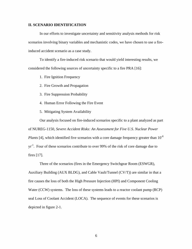
Three of the scenarios (fires in the Emergency Switchgear Room (ESWGR),
Auxiliary Building (AUX BLDG), and Cable Vault/Tunnel (CV/T)) are similar in that a
fire causes the loss of both the High Pressure Injection (HPI) and Component Cooling
Water (CCW) systems. The loss of these systems leads to a reactor coolant pump (RCP)
seal Loss of Coolant Accident (LOCA). The sequence of events for these scenarios is
depicted in figure 2-1.
7
Figure 2-1: RCP Seal LOCA Sequence of Events
For the ESWGR fire, the core damage frequency equation is given in NUREG-
1150 as follows:
][)( 2211 sasaopGswgr ffffRQCDF += τλ
Where:
CDF = The fire induced core damage frequency for the ESWGR.
swgrλ = The frequency of ESWGR fires (of all sizes and severity).
)( GQ τ = The percentage of fires in the data base where the fire was not
manually extinguished before the COMPBRN predicted time to
critical damage occurred.
opR = The probability that operators will fail to cross connect the HPI system
prior to a RCP seal LOCA. This does not require operators to take
action in the direct vicinity of the fire.
1af = The area ratio within the ESWGR for a small fire where critical
damage occurred. This is calculated by dividing the area in the
ESWGR where a small fire could damage both the HPI and CCW
systems by the total area of the ESWGR.

8
1sf = The severity ratio of small fires (based on generic combustible fuel
loading).
2af = The area ratio within the ESWGR for a large fire where critical
damage occurred. This is calculated by dividing the area in the
ESWGR where a large fire could damage both the HPI and CCW
systems by the total area of the ESWGR.
2sf = The severity ratio of large fires (based on generic combustible fuel
loading).
For the AUX BLDG fire, the core damage frequency equation is given in
NUREG-1150 as follows:
opGsaaux RQffCDF )(τλ=
Where:
CDF = The fire-induced core damage frequency for the AUX BLDG.
auxλ = The frequency of AUX BLDG fires.
af = The area ratio within the AUX BLDG where critical damage
occurred.
sf = The severity ratio for a large fire (based on generic combustible fuel
loading).
)( GQ τ = The percentage of fires within the suppression data base where the fire
was not manually extinguished before the COMPBRN predicted time
to critical damage occurred.
9
opR = The probability that operators will fail to cross connect the HPI system
prior to a RCP seal LOCA. This requires the operator to take
action in the direct vicinity of the fire. Because of this, no recovery
action was allowed until 15 minutes after the fire was extinguished.
For the CV/T fire, the core damage frequency equation is given in NUREG-1150
as follows:
opautoGsacsr RQQffCDF )(τλ=
Where:
CDF = The fire-induced core damage frequency for the CV/T.
csrλ = The frequency of CV/T fires.
af = The area ratio within the CV/T where critical damage
occurred.
sf = The severity ratio (based on generic combustible fuel loading).
)( GQ τ = The percentage of fires in the data base where the fire was not
manually extinguished before the COMPBRN predicted time to
critical damage occurred.
autoQ = The probability of the automatic CO2 system not suppressing the fire
before the COMPBRN predicted time to critical damage occurred.
opR = The probability that operators will fail to cross connect the HPI system
prior to a RCP seal LOCA. This does not require operators to take
action in the direct vicinity of the fire.
10
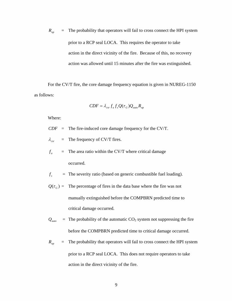
The next scenario is a fire in the Charging Pump Service Water Pump Room
(CPSWPR) that is caused by a general transient followed by a stuck open Power
Operated Relief Valve (PORV) that leads to a small LOCA. The sequence of events for
this scenario is depicted in Figure 2-2.
Figure 2-2: CPSWPR Sequence of Events
For the CPSWPR fire, the core damage frequency equation is as follows:
porvGpr QQCDF )(τλ=
Where:
CDF = The fire-induced core damage frequency for the CPSWPR.
prλ = The frequency of CPSWPR fires.
)( GQ τ = The percentage of fires in the data base where the fire was not
manually extinguished before the COMPBRN predicted time to
critical damage occurred.
porvQ = The probability of having a stuck open PORV with failure to isolate
the leak.
The final fire scenario is a fire in benchboard 1-1 that causes a spurious Power
Operated Relief Valve (PORV) lift and forced Main Control Room (MCR) abandonment
11
followed by failure to recover the plant from the Remote Shutdown Panel (RSP). In this
scenario, PORV indication is not provided at RSP and the PORV “disable” function on
the RSP is not electrically independent from the MCR.
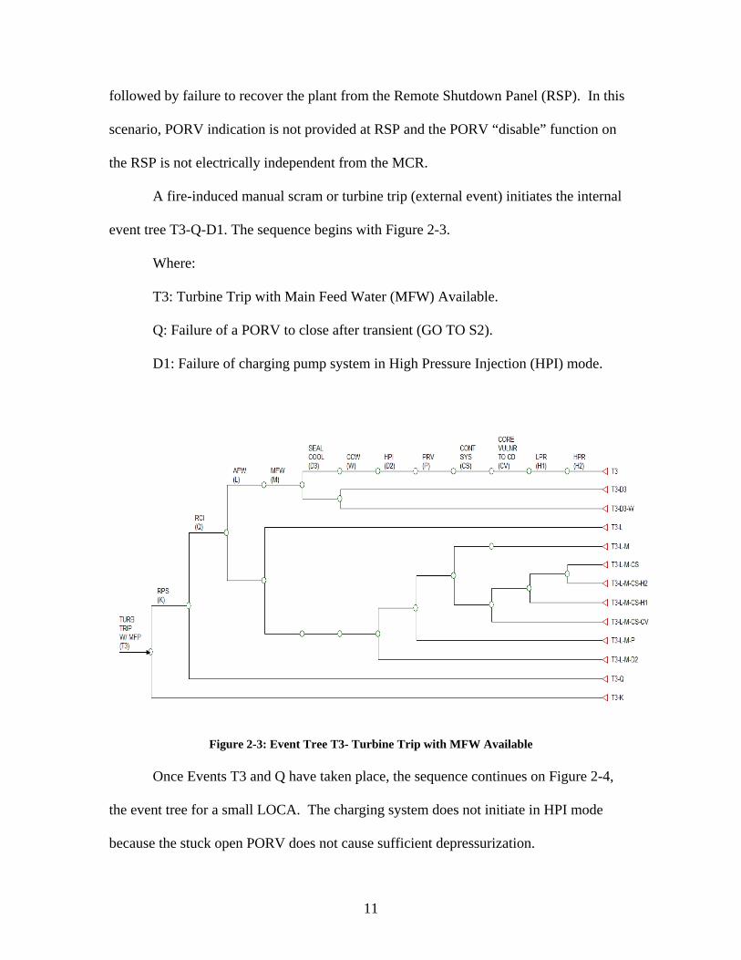
A fire-induced manual scram or turbine trip (external event) initiates the internal
event tree T3-Q-D1. The sequence begins with Figure 2-3.
Where:
T3: Turbine Trip with Main Feed Water (MFW) Available.
Q: Failure of a PORV to close after transient (GO TO S2).
D1: Failure of charging pump system in High Pressure Injection (HPI) mode.
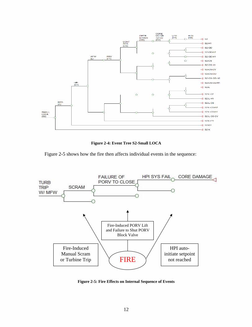
Figure 2-3: Event Tree T3- Turbine Trip with MFW Available Once Events T3 and Q have taken place, the sequence continues on Figure 2-4,
the event tree for a small LOCA. The charging system does not initiate in HPI mode
because the stuck open PORV does not cause sufficient depressurization.
12
Figure 2-4: Event Tree S2-Small LOCA
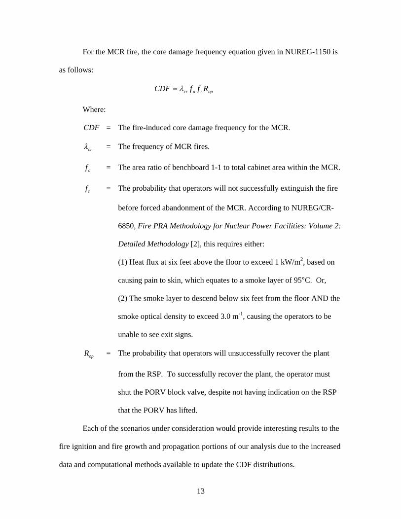
Figure 2-5 shows how the fire then affects individual events in the sequence:
Figure 2-5: Fire Effects on Internal Sequence of Events
FIRE Fire-Induced
Manual Scram or Turbine Trip
HPI auto- initiate setpoint
not reached
Fire-Induced PORV Lift and Failure to Shut PORV
Block Valve
13
For the MCR fire, the core damage frequency equation given in NUREG-1150 is
as follows:
opracr RffCDF λ=
Where:
CDF = The fire-induced core damage frequency for the MCR.
crλ = The frequency of MCR fires.
af = The area ratio of benchboard 1-1 to total cabinet area within the MCR.
rf = The probability that operators will not successfully extinguish the fire
before forced abandonment of the MCR. According to NUREG/CR-
6850, Fire PRA Methodology for Nuclear Power Facilities: Volume 2:
Detailed Methodology [2], this requires either:
(1) Heat flux at six feet above the floor to exceed 1 kW/m2, based on
causing pain to skin, which equates to a smoke layer of 95°C. Or,
(2) The smoke layer to descend below six feet from the floor AND the
smoke optical density to exceed 3.0 m-1, causing the operators to be
unable to see exit signs.
opR = The probability that operators will unsuccessfully recover the plant
from the RSP. To successfully recover the plant, the operator must
shut the PORV block valve, despite not having indication on the RSP
that the PORV has lifted.
Each of the scenarios under consideration would provide interesting results to the
fire ignition and fire growth and propagation portions of our analysis due to the increased
data and computational methods available to update the CDF distributions.
14
Evaluating the non-suppression of fire events is typically done through statistical
methods (Section VIII) involving assessment of the time available for fire suppression
before equipment damage or an operator evacuation threshold is met. These statistical
models are often based on time constants derived from historical fire brigade
performance data and automatic system reliability data. Because the system reliability
data for automatic CO2 systems had to be modified to account for the short time to
critical damage predicted by COMPBRN, the CV/T scenario may not yield interesting
results.
The CPSWPR scenario requires a signal unrelated to the fire to be sent to lift a
PORV and the subsequent failure of the PORV to reclose and isolate the leak. This
factor reduces the CPSWPR scenario Core Damage Frequency (CDF) contribution to less
than one percent of the overall CDF due to fires. Because of this, we have eliminated the
CPSWPR scenario from further consideration.
The ESWGR, CV/T and CPSWPR scenarios do not require human failure events
under increased stress. Only the AUX BLDG and MCR scenarios rely on operator action
in the vicinity of the fire to mitigate the sequence of events leading to core damage.
The ESWGR, AUX BLDG, and CV/T scenarios analyzed in NUREG-1150 lead
to a RCP seal LOCA. Since NUREG-1150 was published, there have been
improvements implemented in RCP seal technology [18, 19] that may lower the
significance of re-analyzing these scenarios.
Other factors we considered are that NUREG-1824, Verification and Validation
of Selected Fire Models for Nuclear Power Plant Applications [5], specifically covers a
MCR fire scenario and has generated experimental data relating to a MCR of general

15
dimensions. With experimental data available, a Bayesian methodology for determining
model uncertainty appears possible [7].
As we move forward, we intend to investigate methods to analyze uncertainty and
sensitivity in risk scenarios induced by main control room fires.

16
III. FIRE IGNITION FREQUENCY
Since NUREG-1150 was published in 1990, there has been an overall downward
trend in fire ignition frequency, including fires initiated in the MCR. This is expected as
plants have improved fire prevention policies from lessons learned and knowledge
sharing practices. Another significant factor is the decline in cigarette smoking rates
nationwide.
We will now develop a distribution of fire ignition frequencies specific to our
MCR abandonment scenario by applying the most updated data and methods available.
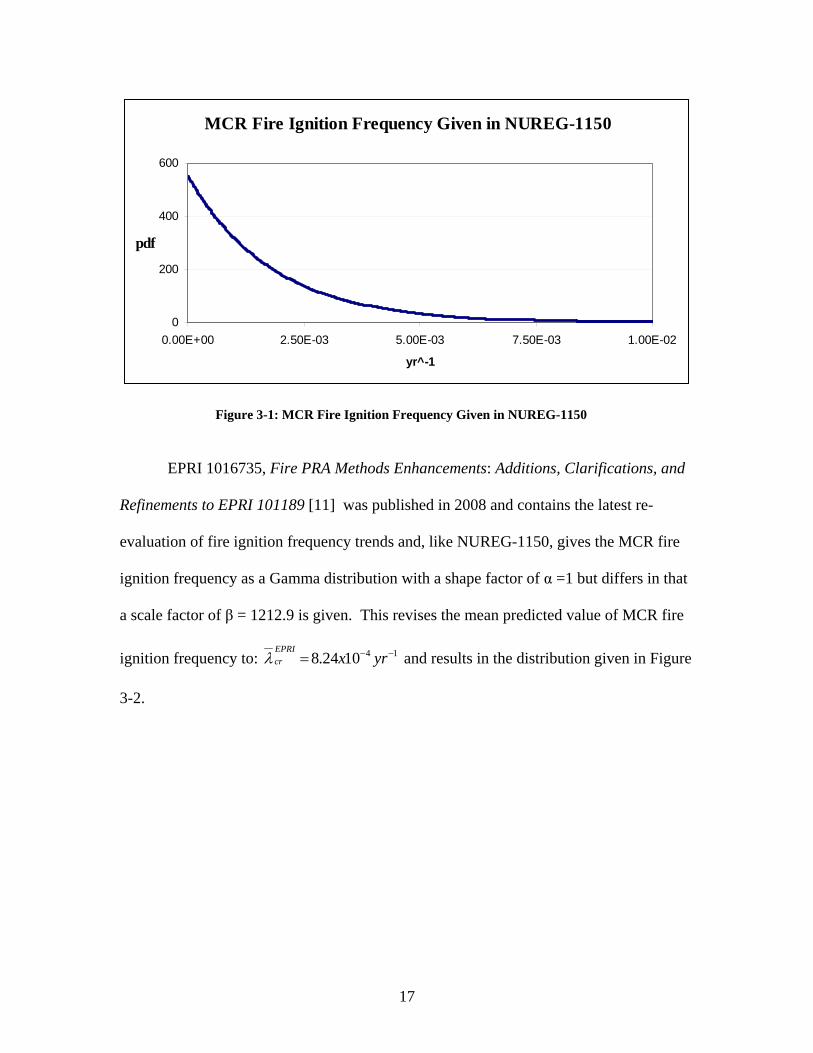
The MCR fire ignition frequency given in the NUREG-1150 analysis is a Gamma
distribution characterized by a shape factor α = 1 and scale factor β = 555.56, such that
the probability density function (pdf) is given by [20]:
)(),|(
/1
αββα α
βα
Γ=
−− xexxf
Where Γ(α) is the Gamma function. The mean value of the Gamma distribution is
αβ-1. Therefore, the mean value of MCR fire ignition frequency is: 131150108.1 −−= yrxcrλ .
The resulting distribution is shown in Figure 3-1.
17
MCR Fire Ignition Frequency Given in NUREG-1150
0
200
400
600
0.00E+00 2.50E-03 5.00E-03 7.50E-03 1.00E-02
yr^-1
Figure 3-1: MCR Fire Ignition Frequency Given in NUREG-1150
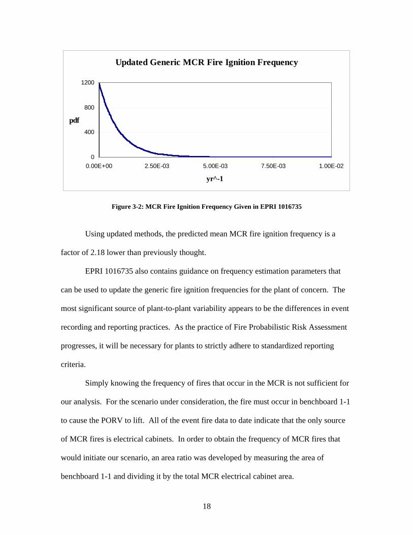
EPRI 1016735, Fire PRA Methods Enhancements: Additions, Clarifications, and
Refinements to EPRI 101189 [11] was published in 2008 and contains the latest re-
evaluation of fire ignition frequency trends and, like NUREG-1150, gives the MCR fire
ignition frequency as a Gamma distribution with a shape factor of α =1 but differs in that
a scale factor of β = 1212.9 is given. This revises the mean predicted value of MCR fire
ignition frequency to: 141024.8 −−= yrxEPRIcrλ and results in the distribution given in Figure
3-2.
18
Updated Generic MCR Fire Ignition Frequency
0
400
800
1200
0.00E+00 2.50E-03 5.00E-03 7.50E-03 1.00E-02
yr̂ -1
Figure 3-2: MCR Fire Ignition Frequency Given in EPRI 1016735
Using updated methods, the predicted mean MCR fire ignition frequency is a
factor of 2.18 lower than previously thought.
EPRI 1016735 also contains guidance on frequency estimation parameters that
can be used to update the generic fire ignition frequencies for the plant of concern. The
most significant source of plant-to-plant variability appears to be the differences in event
recording and reporting practices. As the practice of Fire Probabilistic Risk Assessment
progresses, it will be necessary for plants to strictly adhere to standardized reporting
criteria.
Simply knowing the frequency of fires that occur in the MCR is not sufficient for
our analysis. For the scenario under consideration, the fire must occur in benchboard 1-1
to cause the PORV to lift. All of the event fire data to date indicate that the only source
of MCR fires is electrical cabinets. In order to obtain the frequency of MCR fires that
would initiate our scenario, an area ratio was developed by measuring the area of
benchboard 1-1 and dividing it by the total MCR electrical cabinet area.
19
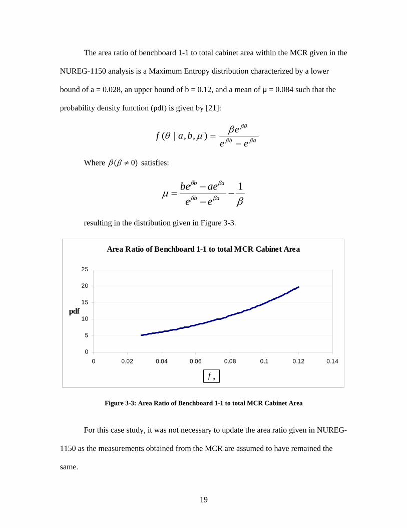
The area ratio of benchboard 1-1 to total cabinet area within the MCR given in the
NUREG-1150 analysis is a Maximum Entropy distribution characterized by a lower
bound of a = 0.028, an upper bound of b = 0.12, and a mean of μ = 0.084 such that the
probability density function (pdf) is given by [21]:
ab eeebaf ββ
βθβμθ−
=),,|(
Where )0( ≠ββ satisfies:
βμ ββ
ββ 1−
−−
= ab
ab
eeaebe
resulting in the distribution given in Figure 3-3.
Area Ratio of Benchboard 1-1 to total MCR Cabinet Area
0
5
10
15
20
25
0 0.02 0.04 0.06 0.08 0.1 0.12 0.14
fa
Figure 3-3: Area Ratio of Benchboard 1-1 to total MCR Cabinet Area
For this case study, it was not necessary to update the area ratio given in NUREG-
1150 as the measurements obtained from the MCR are assumed to have remained the
same.
af
20
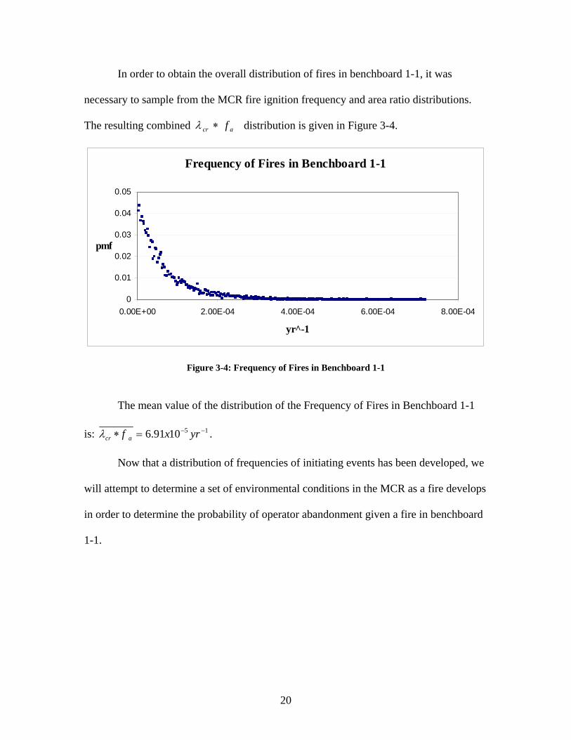
In order to obtain the overall distribution of fires in benchboard 1-1, it was
necessary to sample from the MCR fire ignition frequency and area ratio distributions.
The resulting combined distribution is given in Figure 3-4.
Frequency of Fires in Benchboard 1-1
0
0.01
0.02
0.03
0.04
0.05
0.00E+00 2.00E-04 4.00E-04 6.00E-04 8.00E-04
yr̂ -1
pmf
Figure 3-4: Frequency of Fires in Benchboard 1-1
The mean value of the distribution of the Frequency of Fires in Benchboard 1-1
is: 151091.6 −−=∗ yrxf acrλ .
Now that a distribution of frequencies of initiating events has been developed, we
will attempt to determine a set of environmental conditions in the MCR as a fire develops
in order to determine the probability of operator abandonment given a fire in benchboard
1-1.
acr f∗λ
21
IV. FIRE SCENARIO MODELING
NUREG-1934, Nuclear Power Plant Fire Modeling Application Guide (FMAG) [3], is
currently a draft for public comment that contains guidance on the use of the five fire models
analyzed as a part of NUREG-1824, Verification and Validation of Selected Fire Models for
Nuclear Power Plant Applications [5]. In modeling our MCR abandonment scenario, we
will attempt to apply the guidance contained in NUREG-1934 and NUREG/CR-6850,
EPRI/NRC-RES Fire PRA Methodology for Nuclear Power Facilities: Volume 2:
Detailed Methodology, TASK 11 [2]. Each of these documents contains specific guidance
on the modeling of MCR fires.
Modeling Objectives
In modeling the selected scenario, our objectives are to develop an evolving set of
environmental conditions in the MCR after the start of a fire in benchboard 1-1 in order
to:
1. Assess the length of time the MCR remains habitable in the absence of
suppression efforts by comparing environmental conditions to the MCR abandonment
criteria [2]:
• Heat flux at six feet above the floor to exceed 1 kW/m2, based on
causing pain to skin, which equates to a smoke layer of 95°C.
OR
• The smoke layer to descend below six feet from the floor AND the
smoke optical density to exceed 3.0 m-1, causing the operators to
be unable to see exit signs.
22
2. Provide input to detection and suppression models (Section VIII). In cases
where a MCR abandonment condition is predicted to occur by the model in the absence
of suppression efforts, a probability of non-suppression must be determined through
assessment of the time available for suppression between fire detection and forced
abandonment. In this scenario there are no installed fire suppression systems, but the
MCR is continuously manned. However, because the fire takes place within a
benchboard, no credit is taken for prompt detection. Redundant heat detectors are located
directly above the fire and automatic detection is assumed to occur with a negligible
failure probability.
3. Provide input to Human Reliability Analysis (HRA) models (Section IX). If
the operators fail to suppress the fire and are forced to abandon the MCR, they will be
required to take action from the Remote Shutdown Panel (RSP) under increased stress
and with fewer available indications to prevent core damage.
Fire Model Selection
To identify the optimum model to analyze the scenario under consideration, the
five fire models verified and validated in NUREG-1824 are considered:
(1) Fire Dynamics Tools (FDTs)
(2) Fire-Induced Vulnerability Evaluation, Revision 1 (FIVE-Rev1)
(3) Consolidated Model of Fire Growth and Smoke Transport (CFAST)
(4) MAGIC
(5) Fire Dynamics Simulator (FDS)

23
There are three general types of fire models. FDTs and FIVE-Rev 1 are libraries
of engineering calculations, CFAST and MAGIC are zone models, and FDS is a
computational fluid dynamics model.
Although FDTs and FIVE-Rev 1 provide Hot Gas Layer (HGL) temperature
results, they are not suitable for this scenario because they do not provide smoke
concentration or heat flux data to completely evaluate each of the MCR abandonment
criteria.
FDS results have been shown to be comparable to CFAST and MAGIC,
especially in simple configurations, but are computationally expensive. The single
compartment MCR we will be modeling is a sufficiently simple configuration that a zone
model will provide adequate results. Choosing a zone model allows for much larger
Monte Carlo samples to be reasonably achieved in determining model input parameter
uncertainties (Section VI) and sensitivity analyses (Section X).
In NUREG-1824, CFAST and MAGIC received identical validations for the
outputs of interest in a MCR abandonment scenario. CFAST was chosen over MAGIC
because it is more accessible and is well supported by the National Institute of Standards
and Technology (NIST).
Fire Model Description
According to NUREG-1824, Verification and Validation of Selected Fire Models
for Nuclear Power Plant Applications, Volume 5: Consolidated Fire and Smoke
Transport Model (CFAST) [9]: “CFAST is a two-zone fire model that predicts fire-
induced environmental conditions as a function of time. In order to numerically solve
24
differential equations, CFAST subdivides each compartment into two zones that are
assumed to be uniform in temperature and species concentration.”
The two publications distributed by NIST relevant to CFAST are the CFAST
Technical Reference Guide [22], which explains the assumptions and physics of the
model, and the CFAST User’s Guide [6], which explains how to implement the model.
Fire Model Input
In 1985, Factory Mutual and Sandia National Laboratories (FMSNL) conducted a
series of tests to provide data for use in validating computer fire environment simulation
models, specifically MCR scenarios [8].
One of these tests (FMSNL 21) was conducted in a MCR mock-up with a fire
simulated in a benchboard, similar to the scenario under evaluation. FMSNL 21 was
conducted with a peak Heat Release Rate (HRR) of 470 kW, a value that is estimated to
exceed the peak HRR of greater than 92% of benchboard fires. In addition, the FMSNL
21 test was conducted at a relatively low ventilation rate of one room change per hour.
Sensitivity to these particular input parameters is analyzed in Section X.
Model input was chosen to mimic this test so that the output data could be
compared to experimental results in the development of model uncertainty estimates
(Section V). Inputs specific to the FMSNL 21 test are given in Appendices A, B, and C.
CFAST allows the user to specify the following input parameters:
(1) Ambient Conditions
(2) Compartment dimensions
(3) Construction materials and material properties
(4) Dimensions and positions of flow openings
25
(5) Mechanical ventilation specifications
(6) Sprinkler and detector specifications
(7) Target specifications
(8) Fire properties
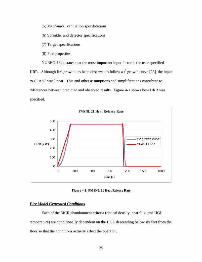
NUREG-1824 states that the most important input factor is the user specified
HRR. Although fire growth has been observed to follow a t2 growth curve [23], the input
to CFAST was linear. This and other assumptions and simplifications contribute to
differences between predicted and observed results. Figure 4-1 shows how HRR was
specified.
FMSNL 21 Heat Release Rate
0
100
200
300
400
500
0 300 600 900 1200 1500 1800
time (s)
HRR (kW)t 2̂ growth curveCFAST HRR
Figure 4-1: FMSNL 21 Heat Release Rate
Fire Model Generated Conditions
Each of the MCR abandonment criteria (optical density, heat flux, and HGL
temperature) are conditionally dependent on the HGL descending below six feet from the
floor so that the conditions actually affect the operator.
26
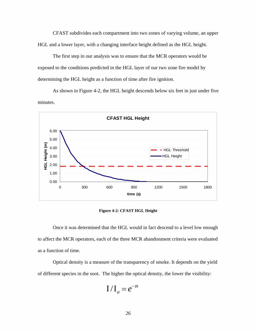
CFAST subdivides each compartment into two zones of varying volume, an upper
HGL and a lower layer, with a changing interface height defined as the HGL height.
The first step in our analysis was to ensure that the MCR operators would be
exposed to the conditions predicted in the HGL layer of our two zone fire model by
determining the HGL height as a function of time after fire ignition.
As shown in Figure 4-2, the HGL height descends below six feet in just under five
minutes.
CFAST HGL Height
0.00
1.00
2.00
3.00
4.00
5.00
6.00
0 300 600 900 1200 1500 1800
time (s)
HG
L H
eigh
t (m
)
HGL ThresholdHGL Height
Figure 4-2: CFAST HGL Height
Once it was determined that the HGL would in fact descend to a level low enough
to affect the MCR operators, each of the three MCR abandonment criteria were evaluated
as a function of time.
Optical density is a measure of the transparency of smoke. It depends on the yield
of different species in the soot. The higher the optical density, the lower the visibility:
xo e τ−=ΙΙ /
27
Where:
I/Io = The fraction of light not scattered or absorbed.
τ = The optical density (units of length-1).
x = The straight line path of length x (units of length).
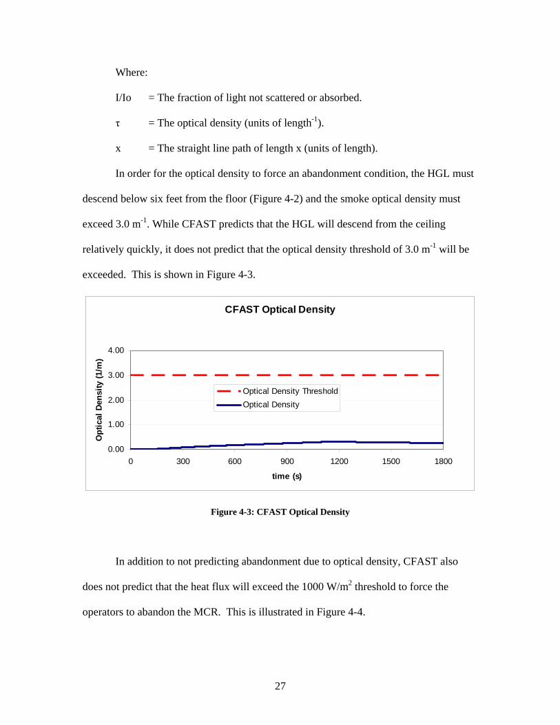
In order for the optical density to force an abandonment condition, the HGL must
descend below six feet from the floor (Figure 4-2) and the smoke optical density must
exceed 3.0 m-1. While CFAST predicts that the HGL will descend from the ceiling
relatively quickly, it does not predict that the optical density threshold of 3.0 m-1 will be
exceeded. This is shown in Figure 4-3.
CFAST Optical Density
0.00
1.00
2.00
3.00
4.00
0 300 600 900 1200 1500 1800
time (s)
Opt
ical
Den
sity
(1/m
)
Optical Density ThresholdOptical Density
Figure 4-3: CFAST Optical Density
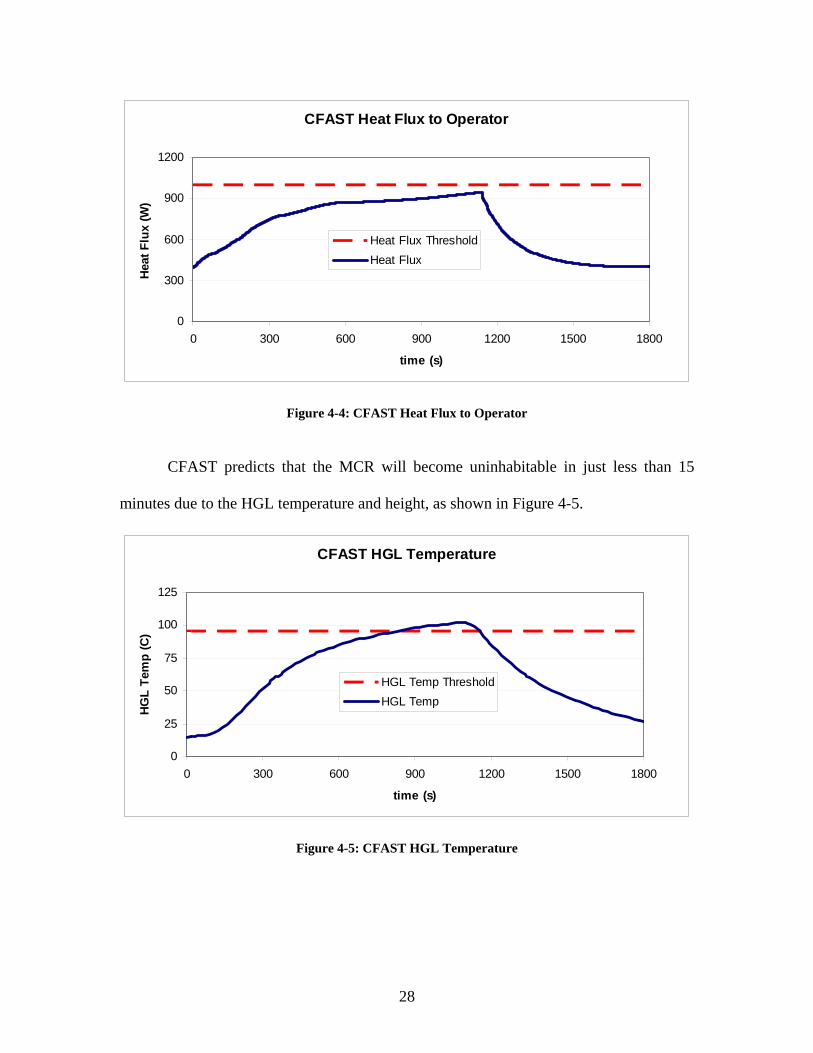
In addition to not predicting abandonment due to optical density, CFAST also
does not predict that the heat flux will exceed the 1000 W/m2 threshold to force the
operators to abandon the MCR. This is illustrated in Figure 4-4.
28
CFAST Heat Flux to Operator
0
300
600
900
1200
0 300 600 900 1200 1500 1800
time (s)
Hea
t Flu
x (W
)
Heat Flux ThresholdHeat Flux
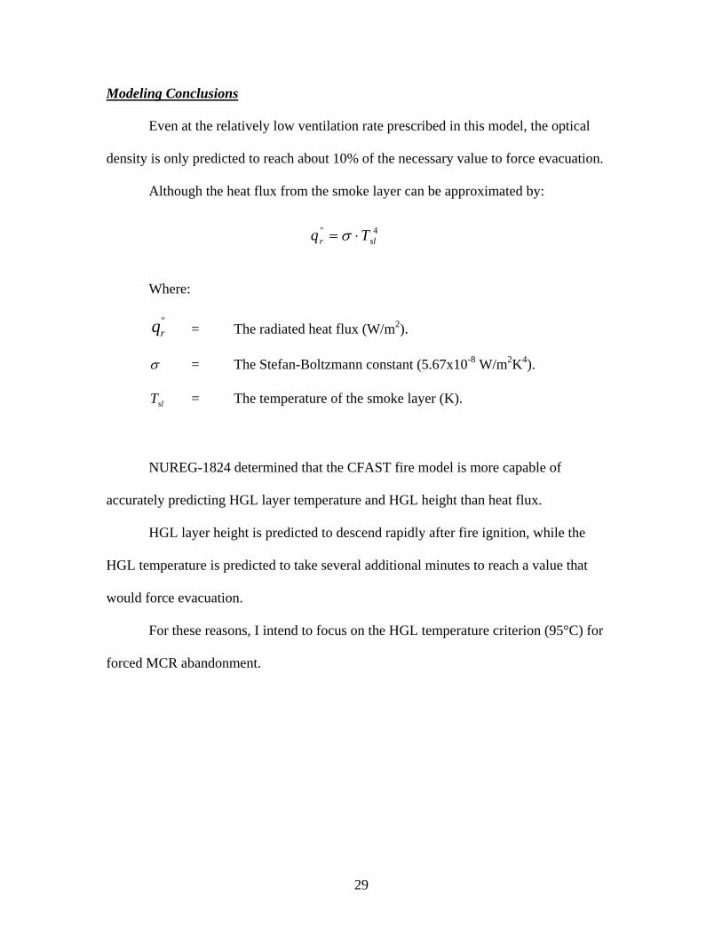
Figure 4-4: CFAST Heat Flux to Operator
CFAST predicts that the MCR will become uninhabitable in just less than 15
minutes due to the HGL temperature and height, as shown in Figure 4-5.
CFAST HGL Temperature
0
25
50
75
100
125
0 300 600 900 1200 1500 1800
time (s)
HG
L Te
mp
(C)
HGL Temp ThresholdHGL Temp
Figure 4-5: CFAST HGL Temperature
29
Modeling Conclusions
Even at the relatively low ventilation rate prescribed in this model, the optical
density is only predicted to reach about 10% of the necessary value to force evacuation.
Although the heat flux from the smoke layer can be approximated by:
Where:
"rq = The radiated heat flux (W/m2).
σ = The Stefan-Boltzmann constant (5.67x10⁻⁸ W/m2K4).
slT = The temperature of the smoke layer (K).
NUREG-1824 determined that the CFAST fire model is more capable of
accurately predicting HGL layer temperature and HGL height than heat flux.
HGL layer height is predicted to descend rapidly after fire ignition, while the
HGL temperature is predicted to take several additional minutes to reach a value that
would force evacuation.
For these reasons, I intend to focus on the HGL temperature criterion (95°C) for
forced MCR abandonment.
4"slr Tq ⋅= σ
30
V. MODEL UNCERTAINTY
Fire growth and propagation contains two primary sources of uncertainty. The
first comes from the input, or parameter, uncertainty that occurs due to the distribution of
the input parameter of interest, such as Heat Release Rate (HRR) (discussed in Section
VI). The other source of uncertainty is the model uncertainty, which is the epistemic
uncertainty resulting from the assumptions and approximations used within the model.
In our model, CFAST, the primary simplification is that each compartment is
divided into two zones that are assumed to have uniform properties. Another
simplification is made by not solving the momentum equation explicitly. However, the
conservation of mass and energy equations are solved as ordinary differential equations.
For our scenario, the primary objective of assessing model uncertainty is to
determine the probability of exceeding the MCR abandonment criterion of interest, HGL
temperature greater than 95 °C, given a model prediction.
The general method of evaluating model uncertainty is through the comparison of
model data with that of actual experiments.
A Bayesian Framework for Model Uncertainty Considerations in Fire Simulation
Codes [7], proposed by the University of Maryland (UMD), was first conducted by
comparing CFAST output to experimental results contained in NUREG-1824’s
Benchmarking Exercise Three (BE3) [9]. Through cooperation with the United States
Nuclear Regulatory Commission (NRC) and the Massachusetts Institute of Technology
(MIT), the UMD method was extended to include data from the FMSNL 21 and 22 tests
conducted as part of NUREG/CR-4527, An Experimental Investigation of Internally
Ignited Fires in Nuclear Power Plant Control Cabinets Part II: Room Effects Tests [8].
31
The results from the UMD method using only the BE3 data (UMD BE3) are
compared to the updated results determined by using the UMD method and including the
FMSNL 21 and 22 test data (UMD BE3 + FMSNL 21/22). The results from the UMD
method are then compared to the method presented in NUREG-1934 (FMAG) [3].
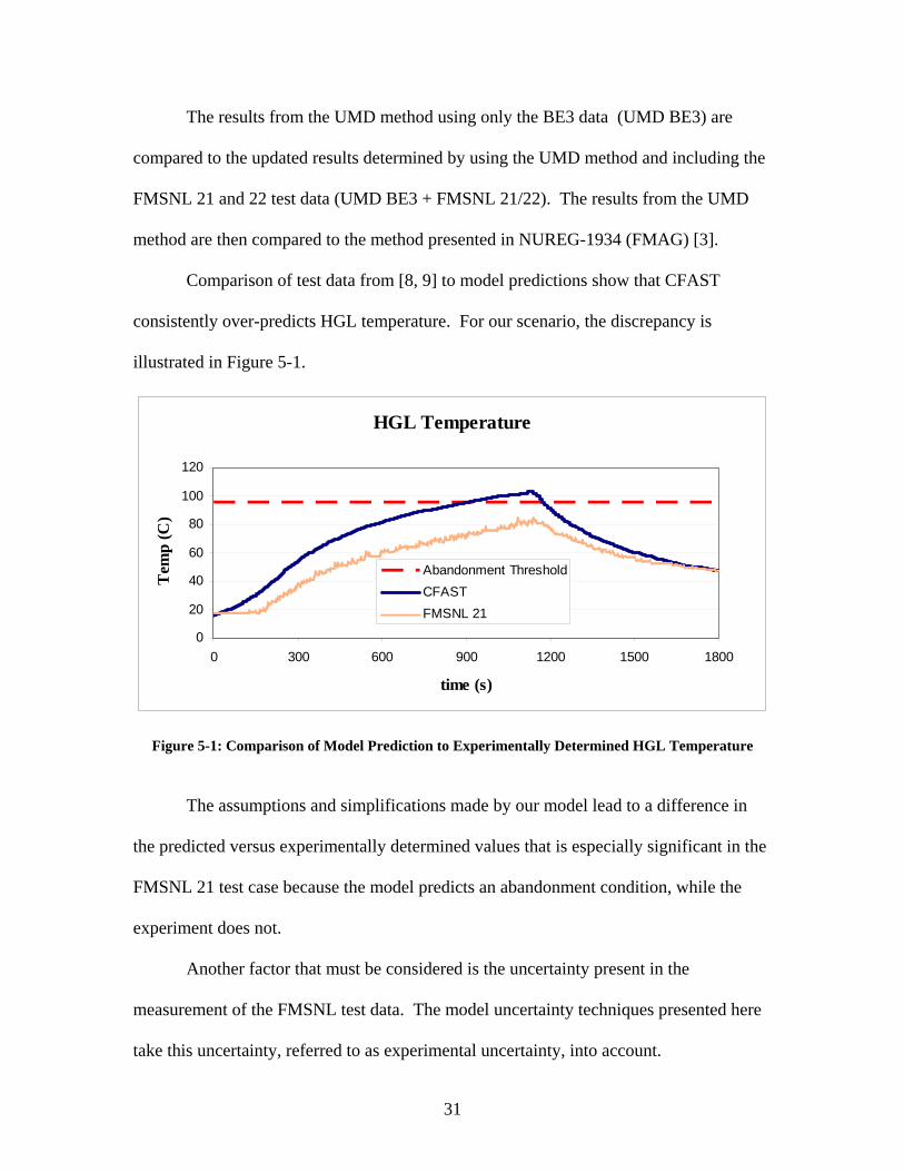
Comparison of test data from [8, 9] to model predictions show that CFAST
consistently over-predicts HGL temperature. For our scenario, the discrepancy is
illustrated in Figure 5-1.
HGL Temperature
0
20
40
60
80
100
120
0 300 600 900 1200 1500 1800
time (s)
Tem
p (C
)
Abandonment ThresholdCFASTFMSNL 21
Figure 5-1: Comparison of Model Prediction to Experimentally Determined HGL Temperature
The assumptions and simplifications made by our model lead to a difference in
the predicted versus experimentally determined values that is especially significant in the
FMSNL 21 test case because the model predicts an abandonment condition, while the
experiment does not.
Another factor that must be considered is the uncertainty present in the
measurement of the FMSNL test data. The model uncertainty techniques presented here
take this uncertainty, referred to as experimental uncertainty, into account.
32
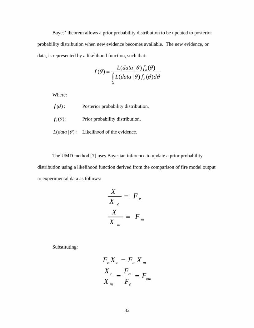
Bayes’ theorem allows a prior probability distribution to be updated to posterior
probability distribution when new evidence becomes available. The new evidence, or
data, is represented by a likelihood function, such that:
∫=
θ
θθθθθ
θdfdataL
fdataLfo
o
)()|()()|()(
Where:
:)(θf Posterior probability distribution.
:)(θof Prior probability distribution.
:)|( θdataL Likelihood of the evidence.
The UMD method [7] uses Bayesian inference to update a prior probability
distribution using a likelihood function derived from the comparison of fire model output
to experimental data as follows:
mm
ee
FXX
FXX
=
=
Substituting:
eme
m
m
e
mmee
FFF
XX
XFXF
==
=

33
Assuming model and experimental errors are independent and log-normally
distributed, the likelihood function to derive the posterior joint distribution of bm and sm
becomes:
( )22, ememem ssbbLNF +−≈
Where:
X: Real quantity of interest.
Xm: Model prediction.
Xe: Result of experiment.
Fm: Multiplicative error of model to real value.
Fe: Multiplicative error of experiment to the real value.
Fem: Multiplicative error of experiment to model prediction.
bm: Mean, error of model to the real value.
be: Mean, error of experiment to the real value.
se: Standard deviation, error of experiment to the real value.
sm: Standard deviation, error of model to the real value.
Once the likelihood function has been developed, the posterior joint distribution
of bm and sm is developed as follows:
∫ ∫ ∗
∗=
m ms bmmmmeememmo
mmeememmoeememm
dsdbsbsbXXLsbfsbsbXXLsbf
sbXXsbf),|,,,(),(
),|,,,(),(),,,|,(
34
Where:
2
122
,
,
22
,
,
)(ln
21exp
2
1),|,,,( ∏=
⎥⎥⎥⎥⎥
⎦
⎤
⎢⎢⎢⎢⎢
⎣
⎡
⎥⎥⎥⎥⎥
⎦
⎤
⎢⎢⎢⎢⎢
⎣
⎡
+
−−⎟⎟⎠
⎞⎜⎜⎝
⎛
−
+⎟⎟⎠
⎞⎜⎜⎝
⎛=
n
i em
emim
ie
emim
iemmeeme ss
bbXX
xss
XX
sbsbXXLπ
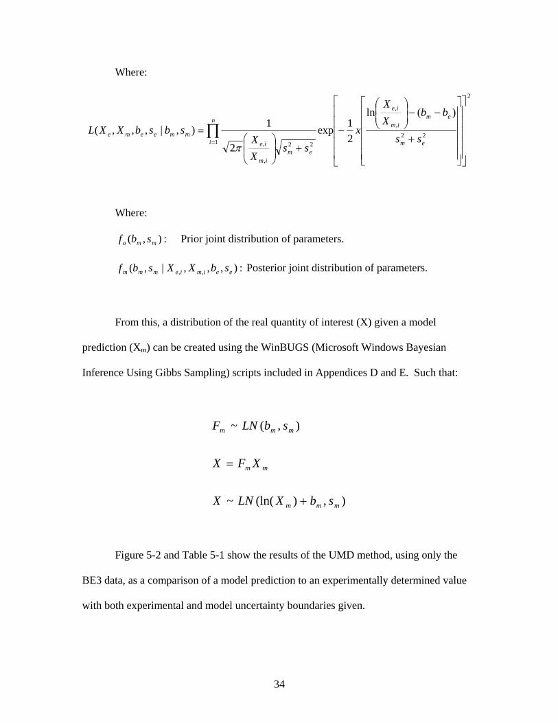
Where:
:),( mmo sbf Prior joint distribution of parameters.
:),,,|,( ,, eeimiemmm sbXXsbf Posterior joint distribution of parameters.
From this, a distribution of the real quantity of interest (X) given a model
prediction (Xm) can be created using the WinBUGS (Microsoft Windows Bayesian
Inference Using Gibbs Sampling) scripts included in Appendices D and E. Such that:
),)(ln(~
),(~
mmm
mm
mmm
sbXLNX
XFX
sbLNF
+
=
Figure 5-2 and Table 5-1 show the results of the UMD method, using only the
BE3 data, as a comparison of a model prediction to an experimentally determined value
with both experimental and model uncertainty boundaries given.
35
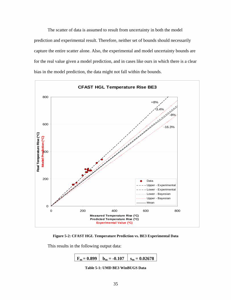
The scatter of data is assumed to result from uncertainty in both the model
prediction and experimental result. Therefore, neither set of bounds should necessarily
capture the entire scatter alone. Also, the experimental and model uncertainty bounds are
for the real value given a model prediction, and in cases like ours in which there is a clear
bias in the model prediction, the data might not fall within the bounds.
CFAST HGL Temperature Rise BE3
0
200
400
600
800
0 200 400 600 800Measured Temperature Rise (°C)Predicted Temperature Rise (°C)
Experimental Value (°C)
Rea
l Tem
pera
ture
Ris
e (°
C)
Mod
el P
redi
ctio
n (°
C)
DataUpper - ExperimentalLower - ExperimentalLower - BayesianUpper - BayesianMean
-8%
+8%
-3.4%
-16.3%
Figure 5-2: CFAST HGL Temperature Prediction vs. BE3 Experimental Data This results in the following output data:
Fm = 0.899 bm = -0.107 sm = 0.02678
Table 5-1: UMD BE3 WinBUGS Data
36
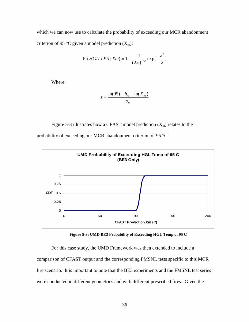
which we can now use to calculate the probability of exceeding our MCR abandonment
criterion of 95 °C given a model prediction (Xm):
]2
exp[)2(
11)|95Pr(2
2/1
zXmHGL −−=>π
Where:
m
mm
sXb
z)ln()95ln( −−
=
Figure 5-3 illustrates how a CFAST model prediction (Xm) relates to the
probability of exceeding our MCR abandonment criterion of 95 °C.
For this case study, the UMD Framework was then extended to include a
comparison of CFAST output and the corresponding FMSNL tests specific to this MCR
fire scenario. It is important to note that the BE3 experiments and the FMSNL test series
were conducted in different geometries and with different prescribed fires. Given the
UMD Probability of Exceeding HGL Temp of 95 C(BE3 Only)
0
0.25
0.5
0.75
1
0 50 100 150 200
CFAST Prediction Xm (C)
CDF
Figure 5-3: UMD BE3 Probability of Exceeding HGL Temp of 95 C
37
assumptions contained within the CFAST model and its known sensitivity to HRR, the
additional data gained from the FMSNL test series may or may not be expected to refine
the uncertainty bounds calculated using only the BE3 test data.
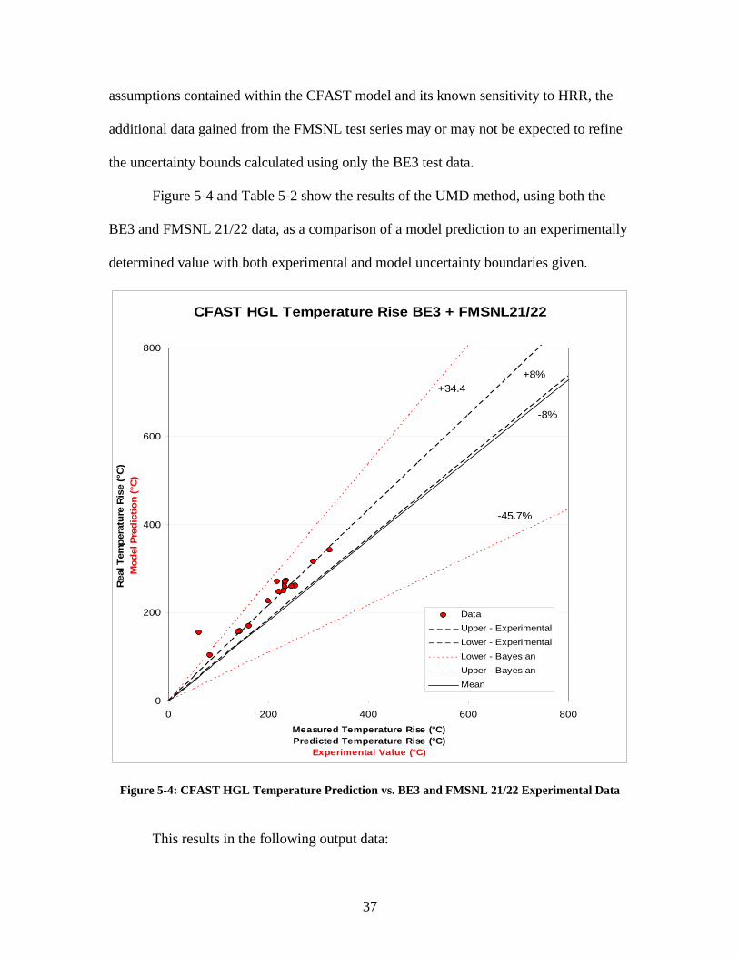
Figure 5-4 and Table 5-2 show the results of the UMD method, using both the
BE3 and FMSNL 21/22 data, as a comparison of a model prediction to an experimentally
determined value with both experimental and model uncertainty boundaries given.
CFAST HGL Temperature Rise BE3 + FMSNL21/22
0
200
400
600
800
0 200 400 600 800Measured Temperature Rise (°C)Predicted Temperature Rise (°C)
Experimental Value (°C)
Rea
l Tem
pera
ture
Ris
e (°
C)
Mod
el P
redi
ctio
n (°
C)
DataUpper - ExperimentalLower - ExperimentalLower - BayesianUpper - BayesianMean
-8%
+8%+34.4
-45.7%
Figure 5-4: CFAST HGL Temperature Prediction vs. BE3 and FMSNL 21/22 Experimental Data
This results in the following output data:
38
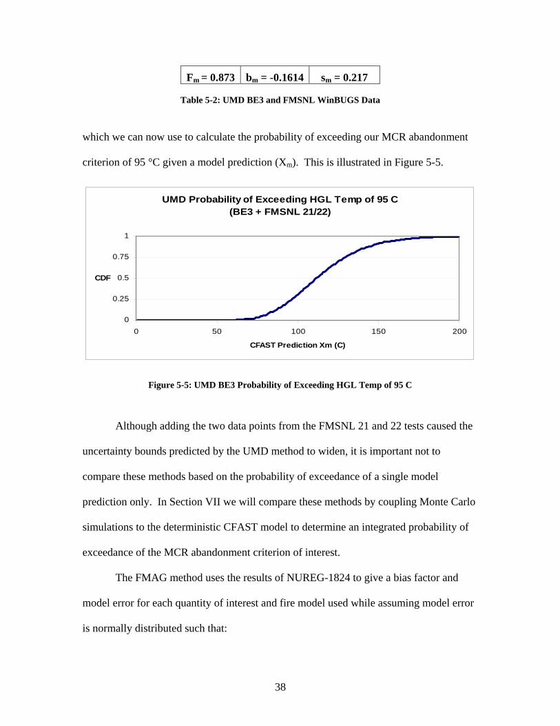
Fm = 0.873 bm = -0.1614 sm = 0.217
Table 5-2: UMD BE3 and FMSNL WinBUGS Data
which we can now use to calculate the probability of exceeding our MCR abandonment
criterion of 95 °C given a model prediction (Xm). This is illustrated in Figure 5-5.
Although adding the two data points from the FMSNL 21 and 22 tests caused the
uncertainty bounds predicted by the UMD method to widen, it is important not to
compare these methods based on the probability of exceedance of a single model
prediction only. In Section VII we will compare these methods by coupling Monte Carlo
simulations to the deterministic CFAST model to determine an integrated probability of
exceedance of the MCR abandonment criterion of interest.
The FMAG method uses the results of NUREG-1824 to give a bias factor and
model error for each quantity of interest and fire model used while assuming model error
is normally distributed such that:
UMD Probability of Exceeding HGL Temp of 95 C(BE3 + FMSNL 21/22)
0
0.25
0.5
0.75
1
0 50 100 150 200
CFAST Prediction Xm (C)
CDF
Figure 5-5: UMD BE3 Probability of Exceeding HGL Temp of 95 C
39
⎥⎦⎤
⎢⎣⎡= )(~,
δσ
δm
mm XXNX
Where:
X: Real quantity of interest.
Xm: Model prediction.
δ: Bias factor.
mσ~ : Relative model error.
For the CFAST model predicting HGL temperature the FMAG gives the
following data:
δ = 1.06 mσ~ = 0.12
Table 5-3: FMAG Data for CFAST Predicting HGL Temperature
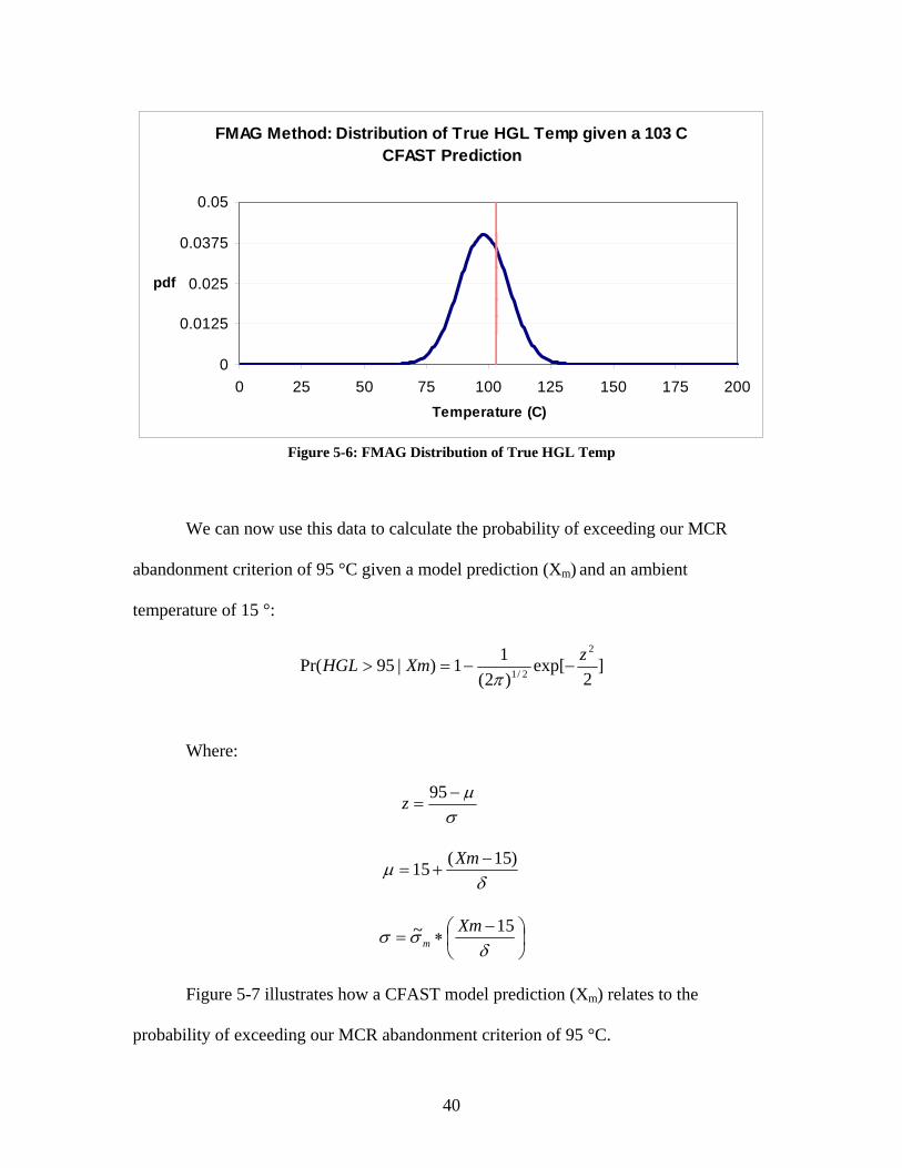
For the FMSNL 21 test case modeled in CFAST and predicting a peak HGL
temperature of 103 °C, this results in a normal distribution with a mean of 98.02 °C and a
standard deviation of 9.96 °C as shown in Figure 5-6.
40
FMAG Method: Distribution of True HGL Temp given a 103 C CFAST Prediction
0
0.0125
0.025
0.0375
0.05
0 25 50 75 100 125 150 175 200Temperature (C)
Figure 5-6: FMAG Distribution of True HGL Temp
We can now use this data to calculate the probability of exceeding our MCR
abandonment criterion of 95 °C given a model prediction (Xm) and an ambient
temperature of 15 °:
]2
exp[)2(
11)|95Pr(2
2/1
zXmHGL −−=>π
Where:
σμ−
=95z
δμ )15(15 −
+=Xm
⎟⎠⎞
⎜⎝⎛ −
∗=δ
σσ 15~ Xmm
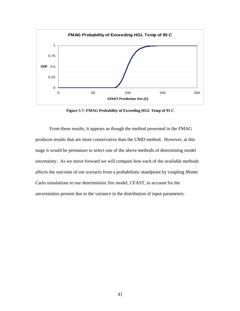
Figure 5-7 illustrates how a CFAST model prediction (Xm) relates to the
probability of exceeding our MCR abandonment criterion of 95 °C.
41
From these results, it appears as though the method presented in the FMAG
produces results that are more conservative than the UMD method. However, at this
stage it would be premature to select one of the above methods of determining model
uncertainty. As we move forward we will compare how each of the available methods
affects the outcome of our scenario from a probabilistic standpoint by coupling Monte
Carlo simulations to our deterministic fire model, CFAST, to account for the
uncertainties present due to the variance in the distribution of input parameters.
FMAG Probability of Exceeding HGL Temp of 95 C
0
0.25
0.5
0.75
1
0 50 100 150 200
CFAST Prediction Xm (C)
CDF
Figure 5-7: FMAG Probability of Exceeding HGL Temp of 95 C
42
VI. PARAMETER UNCERTAINTY
The uncertainty of a model prediction is not only dependent on the assumptions
and simplifications of the model itself, but also on how the uncertainties in input
parameters are propagated throughout the model. Inputs to deterministic fire models are
often not precise values, but instead follow statistical distributions.
In simple cases, when the effect on a single output quantity due to changing just
one input parameter is desired, empirical correlations may be appropriate. NUREG-1934
[3] offers very useful guidance on the use of model-independent empirical correlations
that provide one-to-one mapping of the effect on a specific output quantity given a
change in a single input parameter. For our scenario, where HRR is the most significant
input parameter [9] and the HGL temperature is the output quantity we desire to
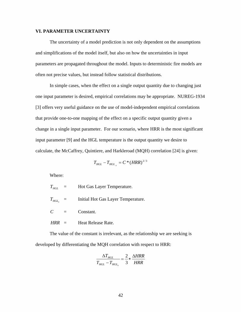
calculate, the McCaffrey, Quintiere, and Harkleroad (MQH) correlation [24] is given:
3/2)(* HRRCTToHGLHGL =−
Where:
HGLT = Hot Gas Layer Temperature.
oHGLT = Initial Hot Gas Layer Temperature.
C = Constant.
HRR = Heat Release Rate.
The value of the constant is irrelevant, as the relationship we are seeking is
developed by differentiating the MQH correlation with respect to HRR:
HRRHRR
TTT
oHGLHGL
HGL Δ∗=
−Δ
32
43
Where:
oHGLHGL
HGL
TTT−
Δ = Relative Change in HGL Temperature Output.
HRRHRRΔ = Relative Change in HRR Parameter Input.
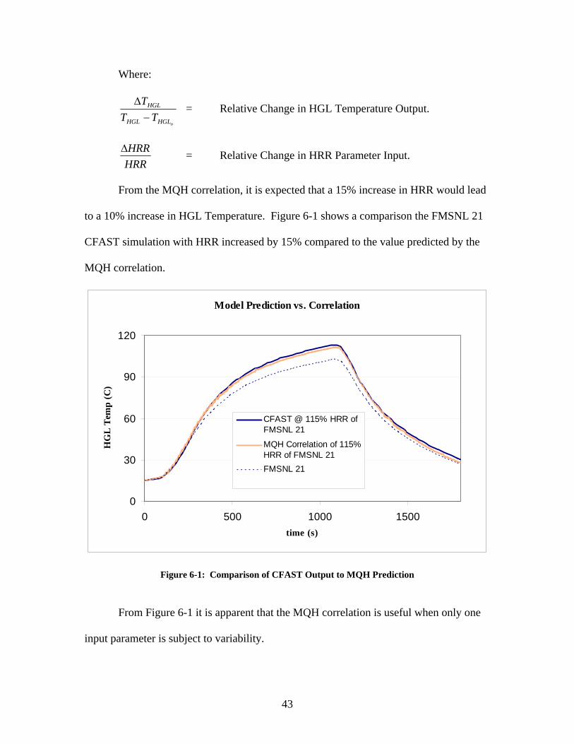
From the MQH correlation, it is expected that a 15% increase in HRR would lead
to a 10% increase in HGL Temperature. Figure 6-1 shows a comparison the FMSNL 21
CFAST simulation with HRR increased by 15% compared to the value predicted by the
MQH correlation.
Model Prediction vs. Correlation
0
30
60
90
120
0 500 1000 1500time (s)
HG
L Te
mp
(C)
CFAST @ 115% HRR ofFMSNL 21
MQH Correlation of 115% HRR of FMSNL 21FMSNL 21
Figure 6-1: Comparison of CFAST Output to MQH Prediction
From Figure 6-1 it is apparent that the MQH correlation is useful when only one
input parameter is subject to variability.
44
Due to the complexity and non-linear nature of our fire model, empirical methods
to estimate uncertainty propagation do not yield sufficiently refined results when multiple
input parameters are allowed to vary. In order to more adequately assess the distributions
of fire model output variables, Monte Carlo simulations have been coupled to our fire
model, CFAST, through a tool called Probabilistic Fire Simulator (PFS) [10]. PFS also
gives the sensitivity of the output variables to the input variables in terms of rank order
correlation coefficients (Section X).
We are primarily concerned with determining the probability that the peak HGL
temperature reached in our MCR fire scenario, as predicted by CFAST, will exceed the
95 °C threshold for MCR abandonment in the absence of suppression efforts. A
secondary goal of interest is to assess the time available for suppression efforts by
comparing the detector activation time with the time of forced abandonment. PFS
provides the necessary time series data for this evaluation.
Once the probability that an abandonment condition in the absence of suppression
efforts has been determined, the parameter uncertainty and model uncertainty results will
be combined (Section VII) to determine an integrated probability of exceeding the
specified abandonment criterion in the absence of suppression efforts.
Suppression efforts will then be factored in through an assessment of the
evolution of environmental conditions in the MCR with time compared to detector
activation data (Section VIII). From this, an estimate of operator abandonment of the
MCR, given a fire in benchboard 1-1, will be obtained.
Prior to fully implementing PFS, it was necessary to first use the spreadsheet
environment to duplicate the modeling results obtained in Section IV in order to
45
demonstrate proper operation. The PFS input specifically designed to mimic the FMSNL
21 test is given in Appendix F.
Once fully implemented, PFS couples Monte Carlo simulations with CFAST in a
spreadsheet environment that allows the user to vary input parameters with individually
specified distributions.
From NUREG-1824 [9] it is known that CFAST is especially sensitive to
variations in HRR. In order to adequately model the HRR distribution during a fire, both
the initial growth period and the fully developed state (HRRmax) must be considered.
Fire growth has been observed to follow a t2 growth curve [23] up to a fully
developed state where the HRR becomes equal to HRRmax, such that:
⎪⎭
⎪⎬⎫
⎪⎩
⎪⎨⎧
⎟⎟⎠
⎞⎜⎜⎝
⎛=
2
max *1000,min)(gttHRRtHRR
Where:
HRR(t) = Heat Release Rate as a function of time.
HRRmax = Maximum HRR attained during the fire scenario.
t = Time after fire ignition.
tg = HRR growth time.
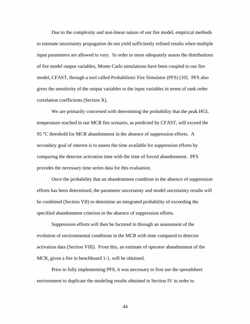
For our scenario, tg is treated as a normally distributed random variable with a
mean of 320 seconds and a standard deviation of 100 seconds, consistent with [10].
Figure 6-2 shows how variations in tg affect the HRR distribution of the FMSNL 21 case.
46
HRR Growth Time Comparison
0
100
200
300
400
500
0 300 600 900 1200 1500 1800
time (s)
HR
R (k
W)
tg=320 s
tg=220 s
tg=420 s
Figure 6-2: Comparison of HRR Distributions Given Variations in Growth Time
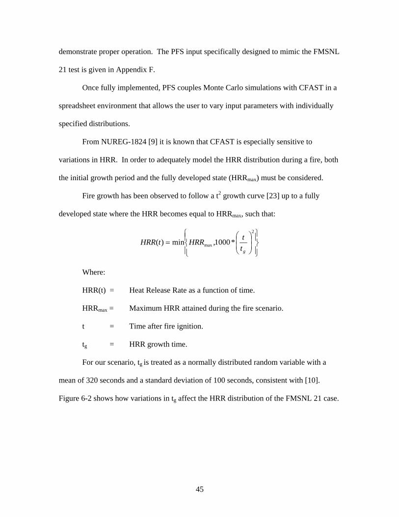
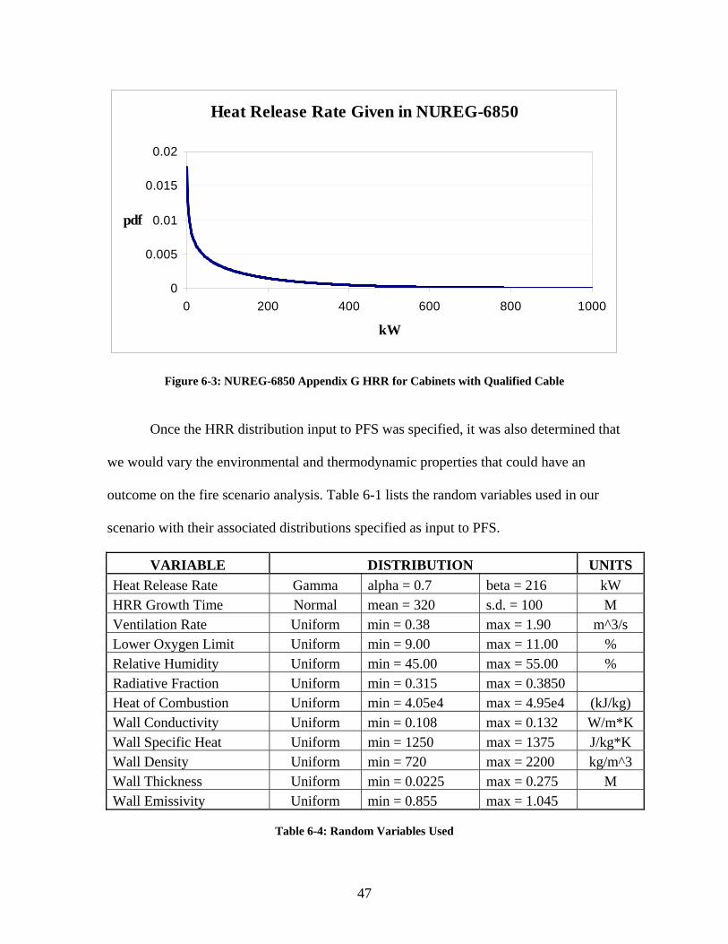
The maximum value that HRR reaches in each simulation (HRRmax) used in this
case study is given in Appendix G of NUREG-6850 [2] as a Gamma distribution
characterized by a shape factor α = 0.7 and scale factor β = 216, such that the probability
density function (pdf) is given by [20]:
)(),|(
/1
αββα α
βα
Γ=
−− xexxf
Where Γ(α) is the Gamma function. The mean value of the distribution is α*β.
The mean value of HRRmax given in Appendix G of NUREG-6850 is:
kWHRR 2.1516850
= resulting in the distribution given in Figure 6-3.
47
Heat Release Rate Given in NUREG-6850
0
0.005
0.01
0.015
0.02
0 200 400 600 800 1000
kW
Figure 6-3: NUREG-6850 Appendix G HRR for Cabinets with Qualified Cable
Once the HRR distribution input to PFS was specified, it was also determined that
we would vary the environmental and thermodynamic properties that could have an
outcome on the fire scenario analysis. Table 6-1 lists the random variables used in our
scenario with their associated distributions specified as input to PFS.
VARIABLE DISTRIBUTION UNITS Heat Release Rate Gamma alpha = 0.7 beta = 216 kW HRR Growth Time Normal mean = 320 s.d. = 100 M Ventilation Rate Uniform min = 0.38 max = 1.90 m^3/s Lower Oxygen Limit Uniform min = 9.00 max = 11.00 % Relative Humidity Uniform min = 45.00 max = 55.00 % Radiative Fraction Uniform min = 0.315 max = 0.3850 Heat of Combustion Uniform min = 4.05e4 max = 4.95e4 (kJ/kg) Wall Conductivity Uniform min = 0.108 max = 0.132 W/m*K Wall Specific Heat Uniform min = 1250 max = 1375 J/kg*K Wall Density Uniform min = 720 max = 2200 kg/m^3 Wall Thickness Uniform min = 0.0225 max = 0.275 M Wall Emissivity Uniform min = 0.855 max = 1.045
Table 6-4: Random Variables Used
48
For each simulation, a CFAST input file is created from both the fixed data and
the samples drawn from random variables within the above constraints. CFAST is then
run to generate and save time series data of the user’s choice for each simulation. For our
scenario it was necessary to generate detector activation time data, HGL temperature time
series data, and a record of the peak HGL temperature achieved in each simulation.
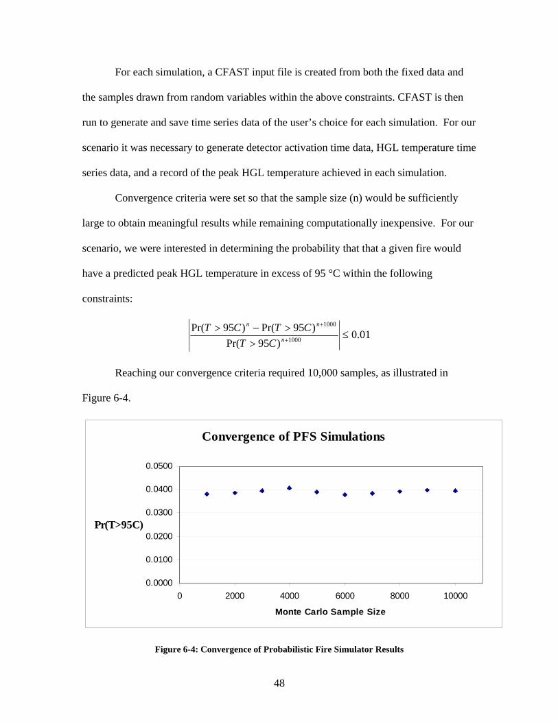
Convergence criteria were set so that the sample size (n) would be sufficiently
large to obtain meaningful results while remaining computationally inexpensive. For our
scenario, we were interested in determining the probability that that a given fire would
have a predicted peak HGL temperature in excess of 95 °C within the following
constraints:
01.0)95Pr(
)95Pr()95Pr(1000
1000
≤>
>−>+
+
n
nn
CTCTCT
Reaching our convergence criteria required 10,000 samples, as illustrated in
Figure 6-4.
Convergence of PFS Simulations
0.0000
0.0100
0.0200
0.0300
0.0400
0.0500
0 2000 4000 6000 8000 10000
Monte Carlo Sample Size
Pr(T>95C)
Figure 6-4: Convergence of Probabilistic Fire Simulator Results
49
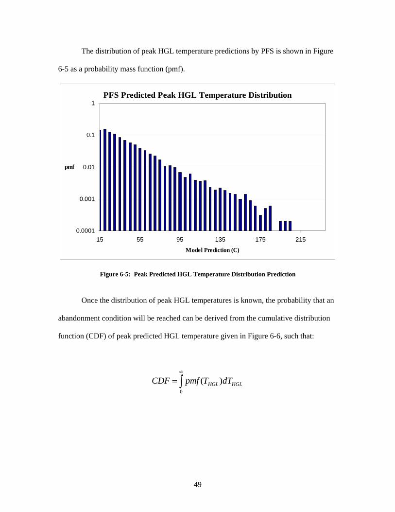
The distribution of peak HGL temperature predictions by PFS is shown in Figure
6-5 as a probability mass function (pmf).
PFS Predicted Peak HGL Temperature Distribution
0.0001
0.001
0.01
0.1
1
15 55 95 135 175 215
Model Prediction (C)
pmf
Figure 6-5: Peak Predicted HGL Temperature Distribution Prediction
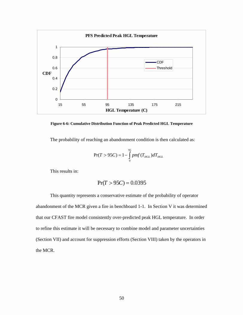
Once the distribution of peak HGL temperatures is known, the probability that an
abandonment condition will be reached can be derived from the cumulative distribution
function (CDF) of peak predicted HGL temperature given in Figure 6-6, such that:
∫∞
=0
)( HGLHGL dTTpmfCDF
50
PFS Predicted Peak HGL Temperature
0
0.2
0.4
0.6
0.8
1
15 55 95 135 175 215HGL Temperature (C)
CDF
CDFThreshold
Figure 6-6: Cumulative Distribution Function of Peak Predicted HGL Temperature
The probability of reaching an abandonment condition is then calculated as:
∫−=>95
0
)(1)95Pr( HGLHGL dTTpmfCT
This results in:
0395.0)95Pr( => CT
This quantity represents a conservative estimate of the probability of operator
abandonment of the MCR given a fire in benchboard 1-1. In Section V it was determined
that our CFAST fire model consistently over-predicted peak HGL temperature. In order
to refine this estimate it will be necessary to combine model and parameter uncertainties
(Section VII) and account for suppression efforts (Section VIII) taken by the operators in
the MCR.
51
VII. COMBINED MODEL AND PARAMETER UNCERTAINTY
Now that we have developed separate techniques for assessing model and
parameter uncertainties, our next task is to combine the methods in an effort to calculate a
cumulative probability of exceeding our MCR abandonment threshold given a fire in
benchboard 1-1 and assuming no suppression efforts are made.
If the only input parameter that we intended to vary was HRR, and if the HRR
distribution was known and normally distributed, we could combine the NUREG-1934
(FMAG) model uncertainty (also normally distributed) and parameter uncertainty via
quadrature, such that [3]:
222 ~~~IM p σσσ +=
Where:
σ~ = The standard deviation of the combined error.
Mσ~ = The standard deviation of the model error.
p = A sensitivity factor (2/3 for HGL temperature).
Iσ~ = The standard deviation of the input (parameter) error.
However, the FMAG method is not applicable to our case study because the
parameter that we are most sensitive to, HRR, is not normally distributed nor is it the
only input parameter to be varied.
In Section V we presented model uncertainty techniques that provide a probability
of exceeding a threshold given a single model prediction, Xm. We will now extend this
framework to handle a distribution of model predictions (Figure 6-5) that is created when
input parameters are allowed to vary as specified in Section VI (Table 6-1).
52
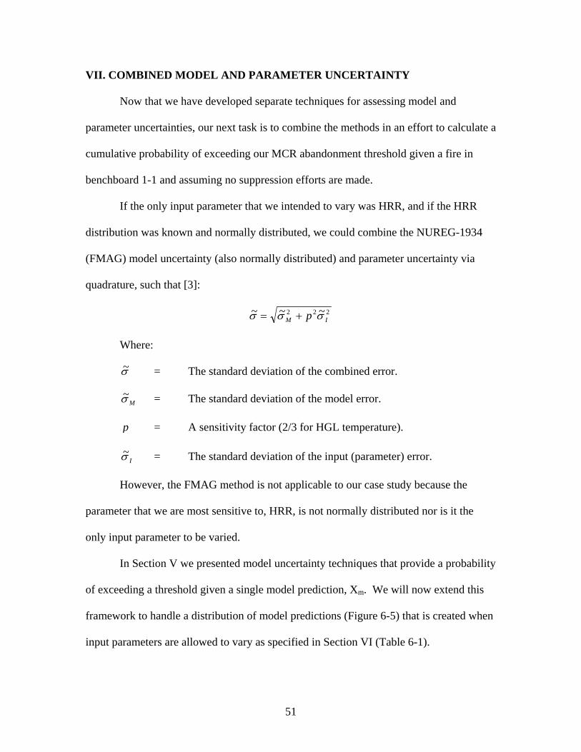
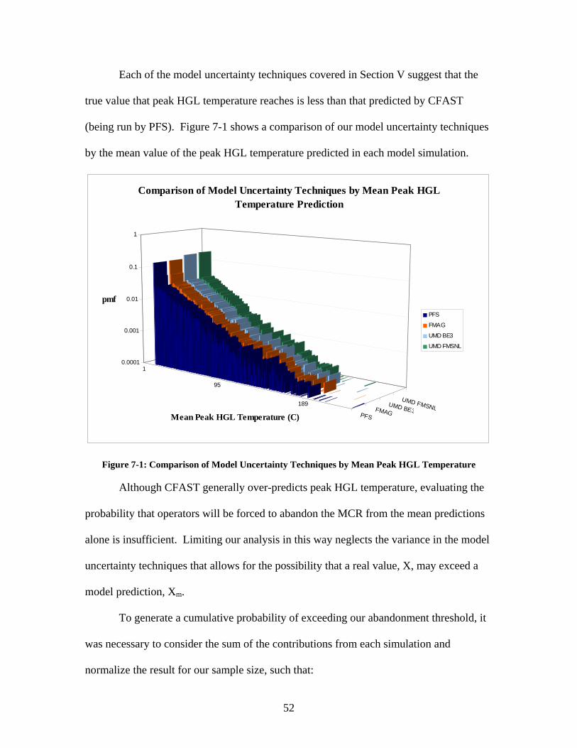
Each of the model uncertainty techniques covered in Section V suggest that the
true value that peak HGL temperature reaches is less than that predicted by CFAST
(being run by PFS). Figure 7-1 shows a comparison of our model uncertainty techniques
by the mean value of the peak HGL temperature predicted in each model simulation.
1
95
189
PFSFMAG
UMD BE3
UMD FMSNL
0.0001
0.001
0.01
0.1
1
pmf
Mean Peak HGL Temperature (C)
Comparison of Model Uncertainty Techniques by Mean Peak HGL Temperature Prediction
PFS
FMAG
UMD BE3
UMD FMSNL
Figure 7-1: Comparison of Model Uncertainty Techniques by Mean Peak HGL Temperature
Although CFAST generally over-predicts peak HGL temperature, evaluating the
probability that operators will be forced to abandon the MCR from the mean predictions
alone is insufficient. Limiting our analysis in this way neglects the variance in the model
uncertainty techniques that allows for the possibility that a real value, X, may exceed a
model prediction, Xm.
To generate a cumulative probability of exceeding our abandonment threshold, it
was necessary to consider the sum of the contributions from each simulation and
normalize the result for our sample size, such that:
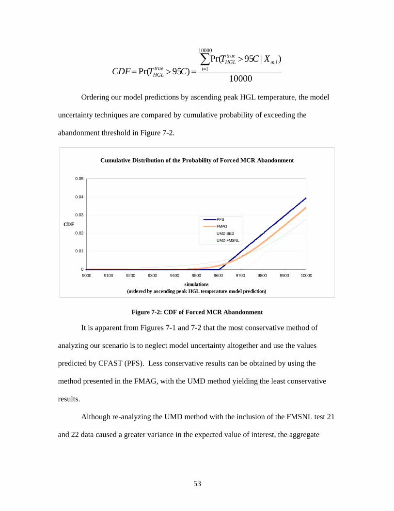
53
10000
)|95Pr()95Pr(
10000
1,∑
=
>=>= i
imtrue
HGLtrue
HGL
XCTCTCDF
Ordering our model predictions by ascending peak HGL temperature, the model
uncertainty techniques are compared by cumulative probability of exceeding the
abandonment threshold in Figure 7-2.
Cumulative Distribution of the Probability of Forced MCR Abandonment
0
0.01
0.02
0.03
0.04
0.05
9000 9100 9200 9300 9400 9500 9600 9700 9800 9900 10000
simulations(ordered by ascending peak HGL temperature model prediction)
CDFPFS
FMAG
UMD BE3
UMD FMSNL
Figure 7-2: CDF of Forced MCR Abandonment
It is apparent from Figures 7-1 and 7-2 that the most conservative method of
analyzing our scenario is to neglect model uncertainty altogether and use the values
predicted by CFAST (PFS). Less conservative results can be obtained by using the
method presented in the FMAG, with the UMD method yielding the least conservative
results.
Although re-analyzing the UMD method with the inclusion of the FMSNL test 21
and 22 data caused a greater variance in the expected value of interest, the aggregate
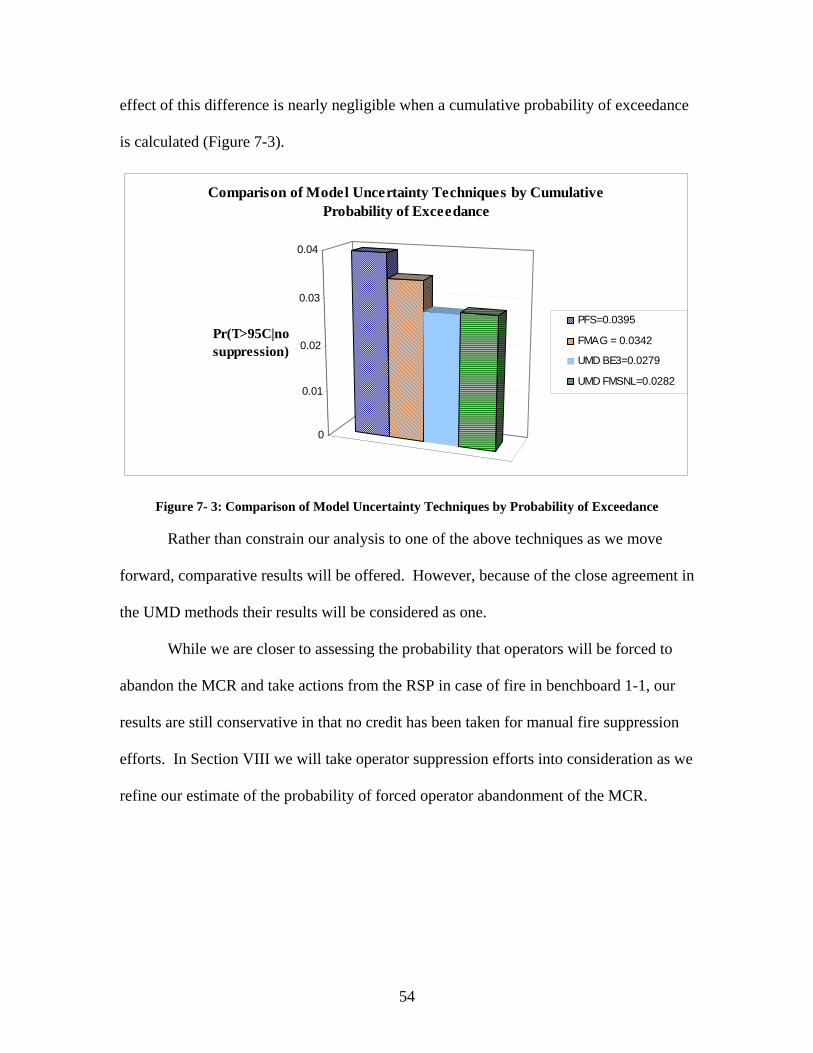
54
effect of this difference is nearly negligible when a cumulative probability of exceedance
is calculated (Figure 7-3).
0
0.01
0.02
0.03
0.04
Pr(T>95C|no suppression)
Comparison of Model Uncertainty Techniques by Cumulative Probability of Exceedance
PFS=0.0395
FMAG = 0.0342
UMD BE3=0.0279
UMD FMSNL=0.0282
Figure 7- 3: Comparison of Model Uncertainty Techniques by Probability of Exceedance
Rather than constrain our analysis to one of the above techniques as we move
forward, comparative results will be offered. However, because of the close agreement in
the UMD methods their results will be considered as one.
While we are closer to assessing the probability that operators will be forced to
abandon the MCR and take actions from the RSP in case of fire in benchboard 1-1, our
results are still conservative in that no credit has been taken for manual fire suppression
efforts. In Section VIII we will take operator suppression efforts into consideration as we
refine our estimate of the probability of forced operator abandonment of the MCR.
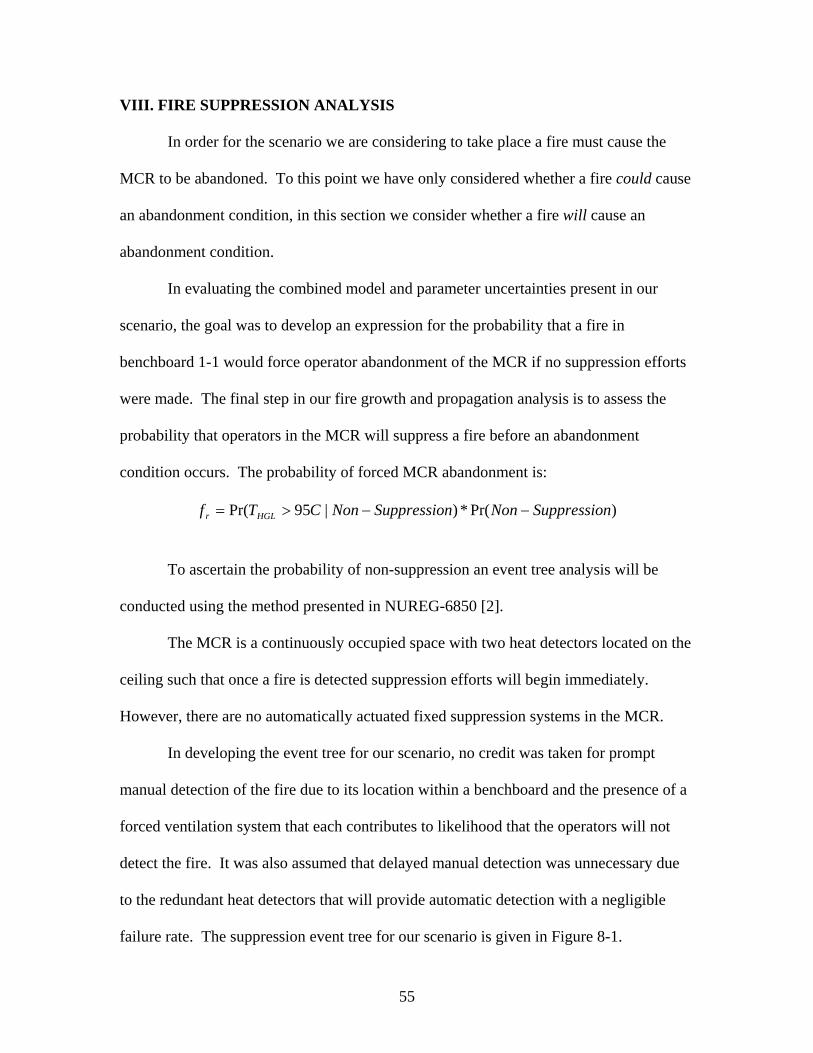
55
VIII. FIRE SUPPRESSION ANALYSIS
In order for the scenario we are considering to take place a fire must cause the
MCR to be abandoned. To this point we have only considered whether a fire could cause
an abandonment condition, in this section we consider whether a fire will cause an
abandonment condition.
In evaluating the combined model and parameter uncertainties present in our
scenario, the goal was to develop an expression for the probability that a fire in
benchboard 1-1 would force operator abandonment of the MCR if no suppression efforts
were made. The final step in our fire growth and propagation analysis is to assess the
probability that operators in the MCR will suppress a fire before an abandonment
condition occurs. The probability of forced MCR abandonment is:
)Pr(*)|95Pr( nSuppressioNonnSuppressioNonCTf HGLr −−>=
To ascertain the probability of non-suppression an event tree analysis will be
conducted using the method presented in NUREG-6850 [2].
The MCR is a continuously occupied space with two heat detectors located on the
ceiling such that once a fire is detected suppression efforts will begin immediately.
However, there are no automatically actuated fixed suppression systems in the MCR.
In developing the event tree for our scenario, no credit was taken for prompt
manual detection of the fire due to its location within a benchboard and the presence of a
forced ventilation system that each contributes to likelihood that the operators will not
detect the fire. It was also assumed that delayed manual detection was unnecessary due
to the redundant heat detectors that will provide automatic detection with a negligible
failure rate. The suppression event tree for our scenario is given in Figure 8-1.
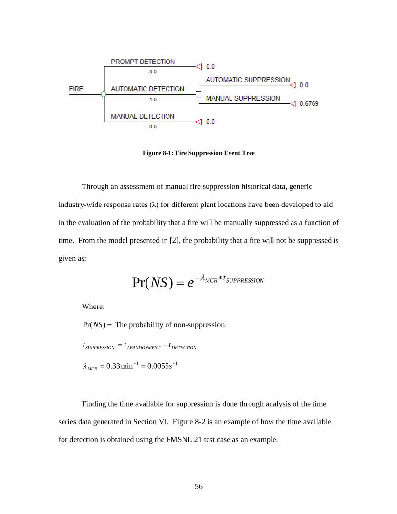
56
Figure 8-1: Fire Suppression Event Tree
Through an assessment of manual fire suppression historical data, generic
industry-wide response rates (λ) for different plant locations have been developed to aid
in the evaluation of the probability that a fire will be manually suppressed as a function of
time. From the model presented in [2], the probability that a fire will not be suppressed is
given as:
NSUPPRESSIOMCR teNS ∗−= λ)Pr(
Where:
=)Pr(NS The probability of non-suppression.
DETECTIONTABANDONMENNSUPPRESSIO ttt −=
11 0055.0min33.0 −− == sMCRλ
Finding the time available for suppression is done through analysis of the time
series data generated in Section VI. Figure 8-2 is an example of how the time available
for detection is obtained using the FMSNL 21 test case as an example.
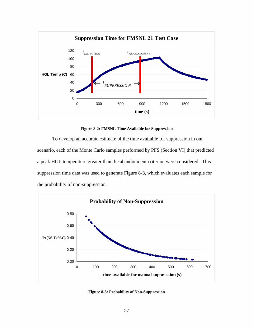
57
Suppression Time for FMSNL 21 Test Case
0
20
40
60
80
100
120
0 300 600 900 1200 1500 1800
time (s)
HGL Temp (C)
Figure 8-2: FMSNL Time Available for Suppression
To develop an accurate estimate of the time available for suppression in our
scenario, each of the Monte Carlo samples performed by PFS (Section VI) that predicted
a peak HGL temperature greater than the abandonment criterion were considered. This
suppression time data was used to generate Figure 8-3, which evaluates each sample for
the probability of non-suppression.
Probability of Non-Suppression
0.00
0.20
0.40
0.60
0.80
0 100 200 300 400 500 600 700
time available for manual suppression (s)
Pr(NS|T>95C)
Figure 8-3: Probability of Non-Suppression
DETECTIONt
→← NSUPPRESSIOt
TABANDONMENt
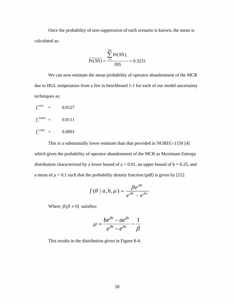
58
Once the probability of non-suppression of each scenario is known, the mean is
calculated as:
3231.0395
)Pr()Pr(
395
1 ==∑=i
iNSNS
We can now estimate the mean probability of operator abandonment of the MCR
due to HGL temperature from a fire in benchboard 1-1 for each of our model uncertainty
techniques as:
PFSrf = 0.0127
FMAGrf = 0.0111
UMDrf = 0.0091
This is a substantially lower estimate than that provided in NUREG-1150 [4]
which gives the probability of operator abandonment of the MCR as Maximum Entropy
distribution characterized by a lower bound of a = 0.01, an upper bound of b = 0.25, and
a mean of μ = 0.1 such that the probability density function (pdf) is given by [21]:
ab eeebaf ββ
βθβμθ−
=),,|(
Where )0( ≠ββ satisfies:
βμ ββ
ββ 1−
−−
= ab
ab
eeaebe
This results in the distribution given in Figure 8-4.
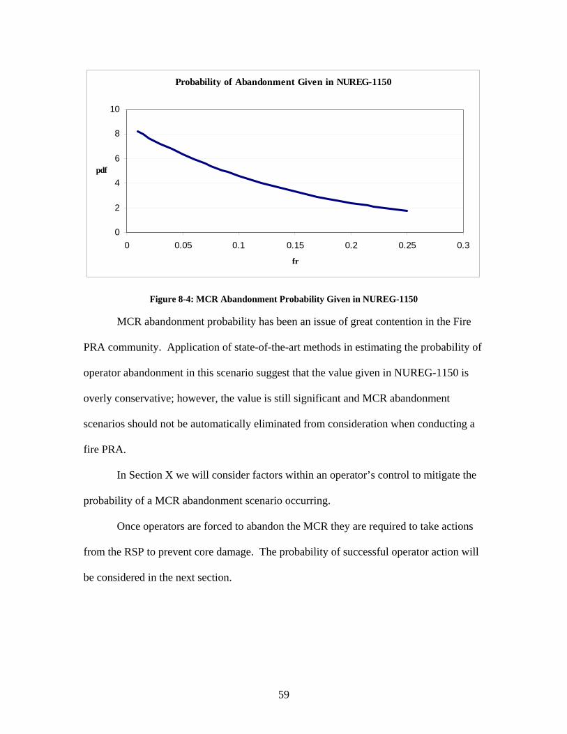
59
Probability of Abandonment Given in NUREG-1150
0
2
4
6
8
10
0 0.05 0.1 0.15 0.2 0.25 0.3
fr
Figure 8-4: MCR Abandonment Probability Given in NUREG-1150
MCR abandonment probability has been an issue of great contention in the Fire
PRA community. Application of state-of-the-art methods in estimating the probability of
operator abandonment in this scenario suggest that the value given in NUREG-1150 is
overly conservative; however, the value is still significant and MCR abandonment
scenarios should not be automatically eliminated from consideration when conducting a
fire PRA.
In Section X we will consider factors within an operator’s control to mitigate the
probability of a MCR abandonment scenario occurring.
Once operators are forced to abandon the MCR they are required to take actions
from the RSP to prevent core damage. The probability of successful operator action will
be considered in the next section.
60
IX. HUMAN RELIABILITY ANALYSIS
After the fire in benchboard 1-1 causes spurious actuation of a PORV and the
operators are forced to abandon the MCR and station themselves at the RSP, they must
shut the PORV block valve to prevent core damage. A low probability of successful
operator action is expected due to the PORV closure status not being displayed on the
RSP and the PORV block valve controls on the RSP not being electrically independent of
the MCR benchboard where the fire is occurring.
NUREG-1921, EPRI RES Fire Human Reliability Analysis Guidelines [12], is
currently a draft for public comment that provides guidance on estimating Human Error
Probabilities (HEPs) for Human Failure Events (HFEs). Three general methods are given
for analyzing post-fire human error probability:
(1) Screening HRA Quantification
(2) Scoping HRA Quantification
(3) Detailed HRA Quantification
These methods are sequentially less conservative and more detailed.
The screening method is the simplest and most conservative of the methods and is
often used as a first step in determining which sequences warrant further consideration.
The scoping method is less conservative than the screening method and uses decision tree
logic to assign appropriate HEPs. Detailed HEP quantification can be accomplished
through the use of the EPRI HRA CALCULATOR [25] or NUREG-1880, A Technique for
Human Event Analysis (ATHEANA) [26]. Both of the detailed quantification methods
require in-depth analysis of plant specific training information and procedures that are
beyond the scope of this generalized report.

61
The screening method of quantifying HEPs has a specific category assigned to
assess the actions taken subsequent to the abandonment of the MCR. For these actions a
global screening value of 1.0 is assigned. It is acknowledged that this is a conservative
estimate and that more detailed analysis should be performed for MCR abandonment
scenarios.
The scoping method introduced in NUREG-1921 offers a method of performing a
less conservative, but still simplified, analysis by taking into account how specific aspects
of the fire scenario determine operator performance. Using the decision-tree format
presented in NUREG-1921, it becomes immediately apparent that not having PORV
indication available at the RSP is problematic. For our scenario, the scoping HRA
decision tree simplifies to Figure 9-1.
Figure 9-1: Scoping HRA Analysis for MCR Abandonment Scenario
Individual plants that show susceptibility to MCR abandonment scenarios may be
able to obtain less conservative results using one of the detailed analysis techniques
presented in NUREG-1921. However, for this scenario, the absence of a cue to alert the
operators that a PORV is open and the further complication caused by not having the
PORV block valve controls on the RSP electrically independent of the MCR benchboard
make it difficult to justify taking credit for successful operator action after abandoning
the MCR.
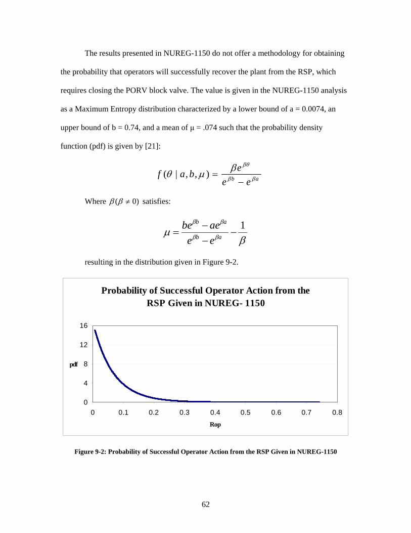
62
The results presented in NUREG-1150 do not offer a methodology for obtaining
the probability that operators will successfully recover the plant from the RSP, which
requires closing the PORV block valve. The value is given in the NUREG-1150 analysis
as a Maximum Entropy distribution characterized by a lower bound of a = 0.0074, an
upper bound of b = 0.74, and a mean of μ = .074 such that the probability density
function (pdf) is given by [21]:
ab eeebaf ββ
βθβμθ−
=),,|(
Where )0( ≠ββ satisfies:
βμ ββ
ββ 1−
−−
= ab
ab
eeaebe
resulting in the distribution given in Figure 9-2.
Probability of Successful Operator Action from the RSP Given in NUREG- 1150
0
4
8
12
16
0 0.1 0.2 0.3 0.4 0.5 0.6 0.7 0.8Rop
Figure 9-2: Probability of Successful Operator Action from the RSP Given in NUREG-1150
63
Although not taking credit for operator actions after forced abandonment of the
MCR revises the total CDF estimate for this scenario upward, the combined effects of
reduced fire ignition frequency and probability of MCR abandonment cause our updated
distribution of CDF for this scenario to be significantly less than the values predicted in
the NUREG-1150 analysis. These results, along with a discussion of the most important
input parameters, will be presented in Section X.
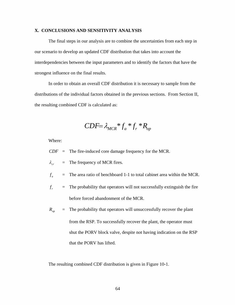
64
X. CONCLUSIONS AND SENSITIVITY ANALYSIS
The final steps in our analysis are to combine the uncertainties from each step in
our scenario to develop an updated CDF distribution that takes into account the
interdependencies between the input parameters and to identify the factors that have the
strongest influence on the final results.
In order to obtain an overall CDF distribution it is necessary to sample from the
distributions of the individual factors obtained in the previous sections. From Section II,
the resulting combined CDF is calculated as:
opraMCR RffCDF ***λ=
Where:
CDF = The fire-induced core damage frequency for the MCR.
crλ = The frequency of MCR fires.
af = The area ratio of benchboard 1-1 to total cabinet area within the MCR.
rf = The probability that operators will not successfully extinguish the fire
before forced abandonment of the MCR.
opR = The probability that operators will unsuccessfully recover the plant
from the RSP. To successfully recover the plant, the operator must
shut the PORV block valve, despite not having indication on the RSP
that the PORV has lifted.
The resulting combined CDF distribution is given in Figure 10-1.
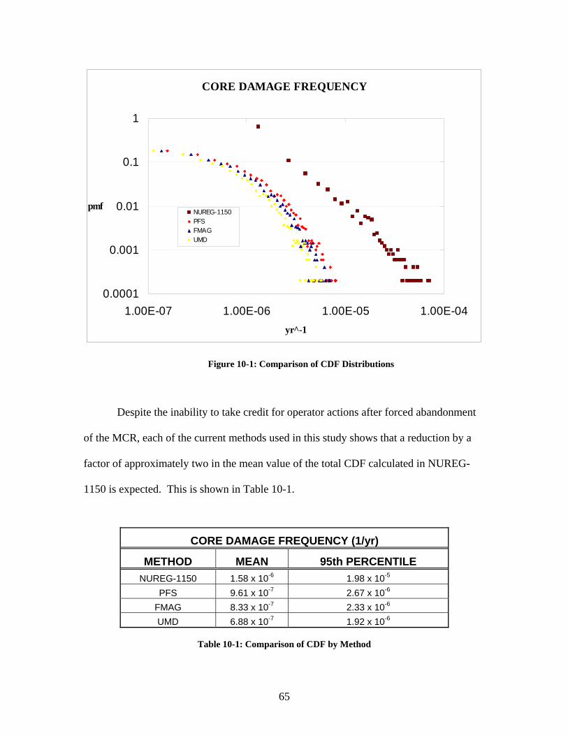
65
CORE DAMAGE FREQUENCY
0.0001
0.001
0.01
0.1
1
1.00E-07 1.00E-06 1.00E-05 1.00E-04yr̂ -1
pmfNUREG-1150PFSFMAGUMD
Figure 10-1: Comparison of CDF Distributions
Despite the inability to take credit for operator actions after forced abandonment
of the MCR, each of the current methods used in this study shows that a reduction by a
factor of approximately two in the mean value of the total CDF calculated in NUREG-
1150 is expected. This is shown in Table 10-1.
CORE DAMAGE FREQUENCY (1/yr)
METHOD MEAN 95th PERCENTILE NUREG-1150 1.58 x 10⁻⁶ 1.98 x 10⁻⁵
PFS 9.61 x 10⁻⁷ 2.67 x 10⁻⁶ FMAG 8.33 x 10⁻⁷ 2.33 x 10⁻⁶ UMD 6.88 x 10⁻⁷ 1.92 x 10⁻⁶
Table 10-1: Comparison of CDF by Method
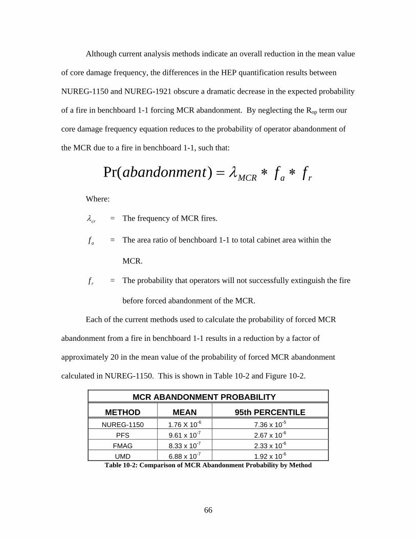
66
Although current analysis methods indicate an overall reduction in the mean value
of core damage frequency, the differences in the HEP quantification results between
NUREG-1150 and NUREG-1921 obscure a dramatic decrease in the expected probability
of a fire in benchboard 1-1 forcing MCR abandonment. By neglecting the Rop term our
core damage frequency equation reduces to the probability of operator abandonment of
the MCR due to a fire in benchboard 1-1, such that:
raMCR fftabandonmen ∗∗= λ)Pr(
Where:
crλ = The frequency of MCR fires.
af = The area ratio of benchboard 1-1 to total cabinet area within the
MCR.
rf = The probability that operators will not successfully extinguish the fire
before forced abandonment of the MCR.
Each of the current methods used to calculate the probability of forced MCR
abandonment from a fire in benchboard 1-1 results in a reduction by a factor of
approximately 20 in the mean value of the probability of forced MCR abandonment
calculated in NUREG-1150. This is shown in Table 10-2 and Figure 10-2.
MCR ABANDONMENT PROBABILITY
METHOD MEAN 95th PERCENTILE NUREG-1150 1.76 X 10⁻⁶ 7.36 x 10⁻⁵
PFS 9.61 x 10⁻⁷ 2.67 x 10⁻⁶ FMAG 8.33 x 10⁻⁷ 2.33 x 10⁻⁶ UMD 6.88 x 10⁻⁷ 1.92 x 10⁻⁶
Table 10-2: Comparison of MCR Abandonment Probability by Method
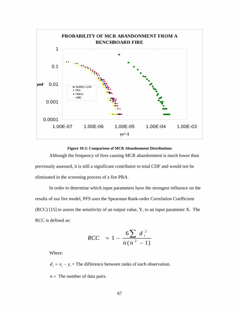
67
PROBABILITY OF MCR ABANDONMENT FROM A BENCHBOARD FIRE
0.0001
0.001
0.01
0.1
1
1.00E-07 1.00E-06 1.00E-05 1.00E-04 1.00E-03yr̂ -1
pmfNUREG-1150PFSFMAGUMD
Figure 10-2: Comparison of MCR Abandonment Distributions
Although the frequency of fires causing MCR abandonment is much lower than
previously assessed, it is still a significant contributor to total CDF and would not be
eliminated in the screening process of a fire PRA.
In order to determine which input parameters have the strongest influence on the
results of our fire model, PFS uses the Spearman Rank-order Correlation Coefficient
(RCC) [15] to assess the sensitivity of an output value, Y, to an input parameter X. The
RCC is defined as:
)1(6
1 2
2
−−= ∑
nnd
RCC i
Where:
iii yxd −= = The difference between ranks of each observation.
=n The number of data pairs.
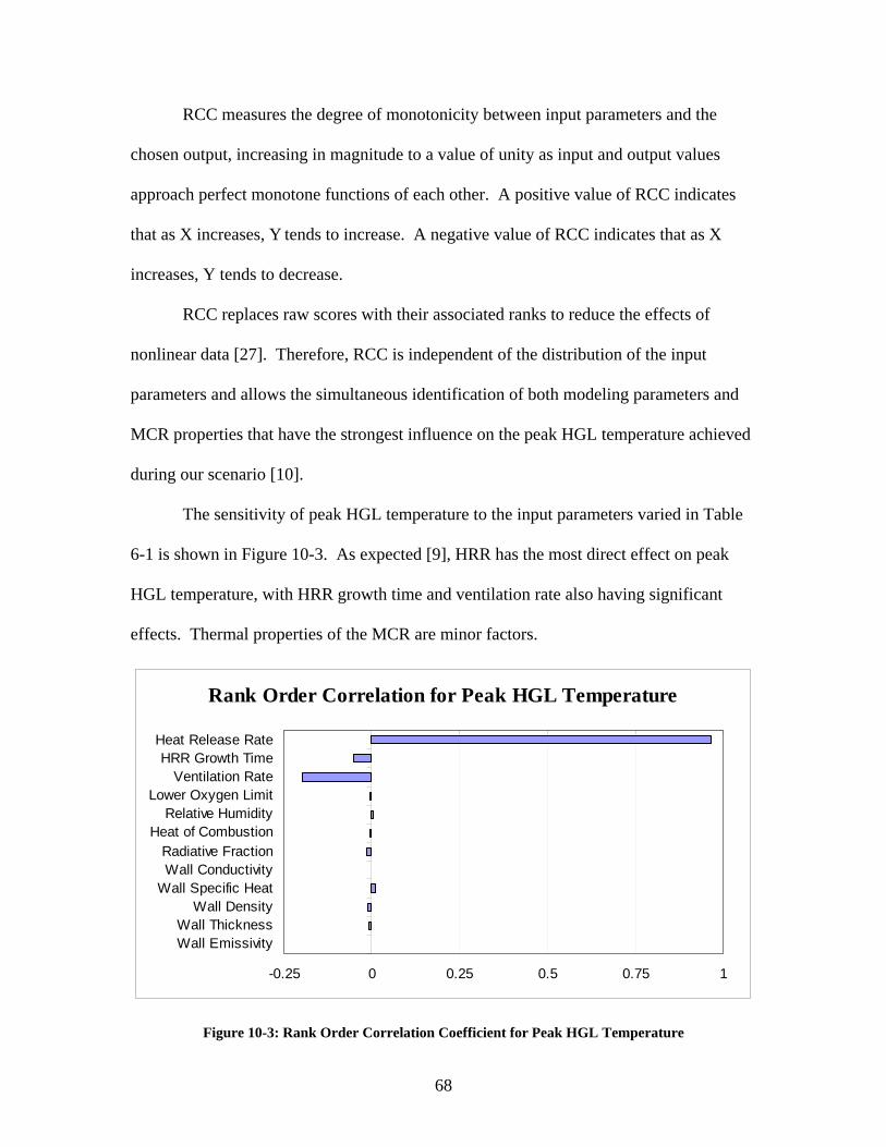
68
RCC measures the degree of monotonicity between input parameters and the
chosen output, increasing in magnitude to a value of unity as input and output values
approach perfect monotone functions of each other. A positive value of RCC indicates
that as X increases, Y tends to increase. A negative value of RCC indicates that as X
increases, Y tends to decrease.
RCC replaces raw scores with their associated ranks to reduce the effects of
nonlinear data [27]. Therefore, RCC is independent of the distribution of the input
parameters and allows the simultaneous identification of both modeling parameters and
MCR properties that have the strongest influence on the peak HGL temperature achieved
during our scenario [10].
The sensitivity of peak HGL temperature to the input parameters varied in Table
6-1 is shown in Figure 10-3. As expected [9], HRR has the most direct effect on peak
HGL temperature, with HRR growth time and ventilation rate also having significant
effects. Thermal properties of the MCR are minor factors.
Rank Order Correlation for Peak HGL Temperature
-0.25 0 0.25 0.5 0.75 1
Heat Release RateHRR Growth Time
Ventilation RateLower Oxygen Limit
Relative HumidityHeat of Combustion
Radiative FractionWall Conductivity
Wall Specific HeatWall Density
Wall ThicknessWall Emissivity
Figure 10-3: Rank Order Correlation Coefficient for Peak HGL Temperature
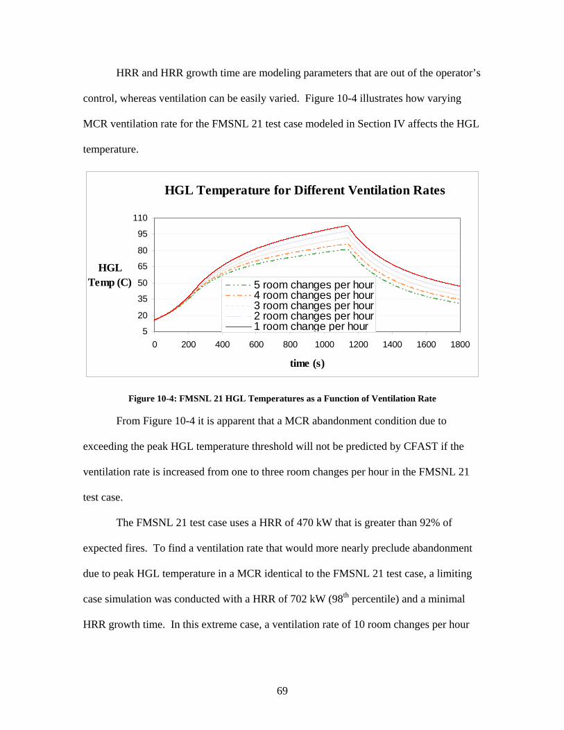
69
HRR and HRR growth time are modeling parameters that are out of the operator’s
control, whereas ventilation can be easily varied. Figure 10-4 illustrates how varying
MCR ventilation rate for the FMSNL 21 test case modeled in Section IV affects the HGL
temperature.
HGL Temperature for Different Ventilation Rates
5
20
35
50
65
80
95
110
0 200 400 600 800 1000 1200 1400 1600 1800
time (s)
HGL Temp (C) 5 room changes per hour
4 room changes per hour3 room changes per hour2 room changes per hour1 room change per hour
Figure 10-4: FMSNL 21 HGL Temperatures as a Function of Ventilation Rate
From Figure 10-4 it is apparent that a MCR abandonment condition due to
exceeding the peak HGL temperature threshold will not be predicted by CFAST if the
ventilation rate is increased from one to three room changes per hour in the FMSNL 21
test case.
The FMSNL 21 test case uses a HRR of 470 kW that is greater than 92% of
expected fires. To find a ventilation rate that would more nearly preclude abandonment
due to peak HGL temperature in a MCR identical to the FMSNL 21 test case, a limiting
case simulation was conducted with a HRR of 702 kW (98th percentile) and a minimal
HRR growth time. In this extreme case, a ventilation rate of 10 room changes per hour
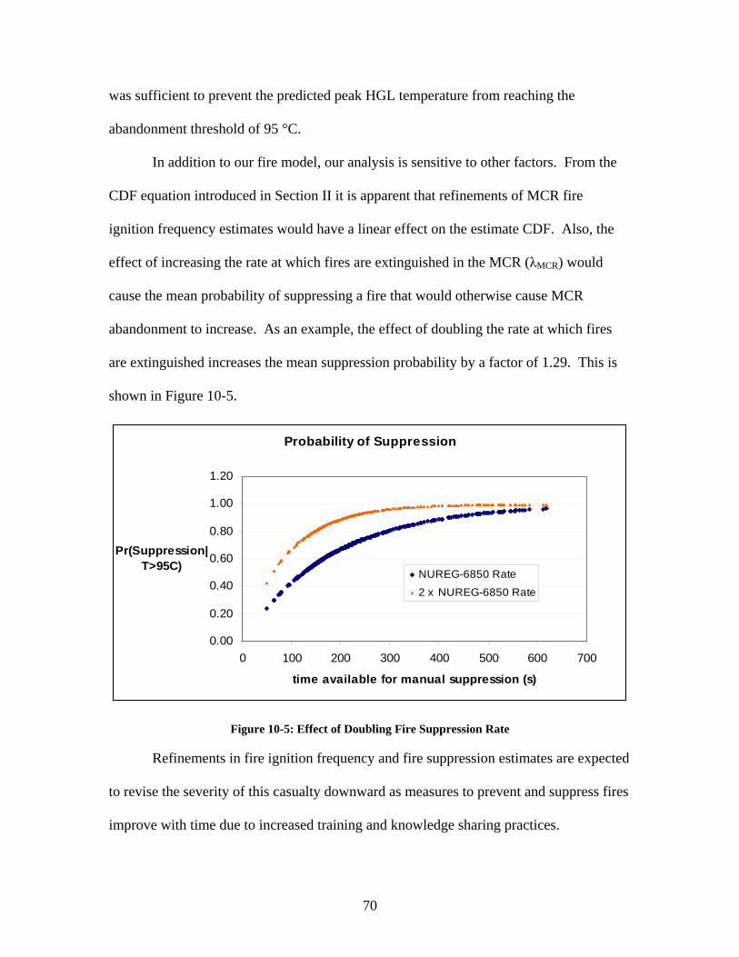
70
was sufficient to prevent the predicted peak HGL temperature from reaching the
abandonment threshold of 95 °C.
In addition to our fire model, our analysis is sensitive to other factors. From the
CDF equation introduced in Section II it is apparent that refinements of MCR fire
ignition frequency estimates would have a linear effect on the estimate CDF. Also, the
effect of increasing the rate at which fires are extinguished in the MCR (λMCR) would
cause the mean probability of suppressing a fire that would otherwise cause MCR
abandonment to increase. As an example, the effect of doubling the rate at which fires
are extinguished increases the mean suppression probability by a factor of 1.29. This is
shown in Figure 10-5.
Probability of Suppression
0.00
0.20
0.40
0.60
0.80
1.00
1.20
0 100 200 300 400 500 600 700
time available for manual suppression (s)
Pr(Suppression|T>95C)
NUREG-6850 Rate
2 x NUREG-6850 Rate
Figure 10-5: Effect of Doubling Fire Suppression Rate
Refinements in fire ignition frequency and fire suppression estimates are expected
to revise the severity of this casualty downward as measures to prevent and suppress fires
improve with time due to increased training and knowledge sharing practices.
71
The scoping method of quantifying the HEP introduced in NUREG-1921[12] is
an adequate and conservative tool for our analysis. For our scenario, the design of the
RSP is the primary factor leading to our conservative HEP estimate of 1.0. If proper
indication were provided to operators once they were forced to abandon the MCR, and if
their required actions did not involve operation of equipment not electrically independent
of the fire, it is likely that the HEP estimate would be reduced by a factor of 2. However,
this analysis would involve a review of plant specific procedures and time margins to
core damage.
The results of our case study indicate that for existing plants the one controllable
factor available to an operator to mitigate the probability of a MCR abandonment
scenario is the MCR ventilation rate.
For plants yet to be constructed, the effects of a MCR casualty could be
substantially reduced through an improved design of the RSP that provides the operators
with the necessary cues and independent circuitry to take actions to terminate this
casualty before core damage occurs.
The results of this study are heavily dependent on the distribution of HRR. The
research into HRR distributions that is currently being conducted will help to provide
regulators with the necessary tools to fully assess the contribution to core damage
frequency from fires initiated from within the MCR.
It is important to note that this work is a limited study meant to apply to a specific
scenario and may not be applicable to all scenarios, such as a complete loss of power or a
fire in a vertical cabinet. PRA practitioners are encouraged to take note of the narrow
range of applicability of the methods and results presented here.
72
REFERENCES
[1] NFPA 805, Performance-Based Standard for Fire Protection for Light Water Reactor Electric Generating Plants, National Fire Protection Association, Quincy, MA, 2001.
[2] EPRI/NRC-RES Fire PRA Methodology for Nuclear Power Facilities: Volume 2: Detailed Methodology. Electric Power Research Institute (EPRI), Palo Alto, CA, and U.S. Nuclear Regulatory Commission, Office of Nuclear Regulatory Research (RES), Rockville, MD: 2005, EPRI TR-1011989 and NUREG/CR- 6850. [3] Nuclear Power Plant Fire Modeling Application Guide (NPP FIRE MAG), U.S. Nuclear Regulatory Commission, Office of Nuclear Regulatory Research (RES), Rockville, MD, 2007, and Electric Power Research Institute (EPRI), Palo Alto, CA, NUREG-1934 and EPRI 1019195. [4] “Severe Accident Risks: An Assessment for Five U.S. Nuclear Power Plants” NUREG-1150, December 1990. [5] Verification and Validation of Selected Fire Models for Nuclear Power Plant Applications ,Volume 1: Main Report, U.S. Nuclear Regulatory Commission, Office of Nuclear Regulatory Research (RES), Rockville, MD, 2007, and Electric Power Research Institute (EPRI), Palo Alto, CA, NUREG-1824 and EPRI 1011999. [6] Peacock, R.D., W.W. Jones, P.A. Reneke, and G.P. Forney, “Consolidated Model of Fire Growth and Smoke Transport (Version 6), User’s Guide,” SP 1041, National Institute of Standards and Technology, Gaithersburg, MD, 2005. [7] Azarkhall, M., Ontiveros, V., Modarres, M., July 2009 “A Bayesian Framework for Model Uncertainty Considerations in Fire Simulation Codes” ICONE17- 75684, Brussels, Belgium. [8] Chavez, J.M.; Nowlen, S.P.; NUREG/CR-4527, SAND86-0336, Vol. 2, “An Experimental Investigation of Internally Ignited Fires in Nuclear Power Plant Control Cabinets Part II: Room Effects Tests”, U.S. Nuclear Regulatory Commission, Washington, DC, and Sandia National Laboratories, Albuquerque, NM, April 1987. [9] Verification and Validation of Selected Fire Models for Nuclear Power Plant Applications, Volume 5: Consolidated Fire and Smoke Transport Model (CFAST), U.S. Nuclear Regulatory Commission, Office of Nuclear Regulatory Research (RES), Rockville, MD, 2007, and Electric Power Research Institute (EPRI), Palo Alto, CA, NUREG-1824 and EPRI 1011999.
73
[10] Hostikka, Simo and Keski-Rahkonen Olavi. Probabilistic Simulation of Fire Scenarios, VTT Building and Transport, PO Box 1803, FIN-02044 VTT, Finland, 2003. [11] Fire PRA Methods Enhancements: Additions, Clarifications, and Refinements to EPRI 1019189. EPRI, Palo Alto, CA: 2008. 1016735. [12] EPRI/NRC-RES Fire Human Reliability Analysis Guidelines), U.S. Nuclear Regulatory Commission, Office of Nuclear Regulatory Research (RES), Rockville, MD, 2007, and Electric Power Research Institute (EPRI), Palo Alto, CA, NUREG-1921 and EPRI 1019196. [13] Saltelli, A., ‘Sensitivity Analysis for Importance Assessment,” Risk Analysis, Vol. 22, 3, pp. 579-590. [14] Saltelli, A., Ratto, M., Andres, T., Campolongo, F., Cariboni, J., Gatelli, D., Saisana, M., Tarantola, S., Global Sensitivity Analysis: The Primer , 2008. [15] C. Spearman, "The proof and measurement of association between two things" Amer. J. Psychol., 15 (1904) pp. 72–101.
[16] Meyer, S. P., July 2009 “Sources of Uncertainty in a Fire Probabilistic Safety Assessment” ICONE17-75360, Brussels, Belgium. [17] “Analysis of Core Damage Frequency: Surry Power Station, Unit 1, External Events” NUREG/CR-4550, Vol. 3, Rev. 1, Part 3, December 1990. [18] WCAP-16396-NP, "Westinghouse Owners Group Reactor Coolant Pump Seal Performance for Appendix R Assessments," Westinghouse Electric Co., January 2005. [19] WCAP-17100-NP, “PRA Model for the Westinghouse Shut Down Seal” Westinghouse Electric Co., July 2009. [20] Atwood, C.L. et al., 2003. Handbook of Parameter Estimation for Probabilistic Risk Assessment, NUREG/CR-6823, U. S. Nuclear Regulatory Commission, September 2003. [21] Siu, N., and D. Kelly, 1998, Bayesian Parameter Estimation in Probabilistic Risk Assessment, in Reliability Engineering and System Safety, Vol. 62, pp. 89-116. [22] Jones, W.W., R.D. Peacock, G.P. Forney, and P.A. Reneke, “Consolidated Model of Fire Growth and Smoke Transport (Version 6): Technical Reference Guide,”
74
NIST SP 1026, National Institute of Standards and Technology, Gaithersburg, MD, 2005. [23] Heskestad, G., Delichatsios, M.A., 1977. Environments of Fire Detectors. Phase 1. Effect of Fire Size, Ceiling Height and Materials. Vol. 2. Analysis. NBS GCR 77-95, National Bureau of Standards. Gaithersburg, MD, 129 pp. [24] Chapter 6; Section 3; NFPA HFPE-02; SFPE Handbook of Fire Protection Engineering. 3rd Edition, DiNenno, P. J.; Drysdale, D.; Beyler, C. L.; Walton, W. D., Editor(s), 3/171-188 p., 2002. Walton, W. D.; Thomas, P. H. [25] Software Users Manual, The Human Reliability Calculator Version 4.0. EPRI, Palo Alto, CA, and Scientech, Tukwila, WA: January 2008. Product ID. 1015358. [26] NUREG-1880, “ATHEANA User’s Guide”, Final Report, U.S. NRC, Washington, DC, June 2007. [27] Hamby, D.M., A Comparison of Sensitivity Analysis Techniques, Health Phys. 1995 Feb; 68(2):195-204.
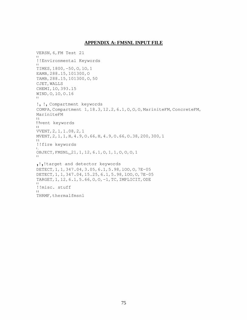
75
APPENDIX A: FMSNL INPUT FILE VERSN,6,FM Test 21 I I
!!Environmental Keywords I I
TIMES,1800,-50,O,lO,1 EAMB,288.15,101300,O TAMB,288.15,101300,O,50 CJET,WALLS CHEMI,lO,393.15 WIND,O,lO,O.16 I I
!, !, Compartment keywords COMPA,Compartment 1,18.3,12.2,6.1,O,O,O,MariniteFM,ConcreteFM, MariniteFM I 1 ! !vent keywords I I VVENT,2,1,1.08,2,1 MVENT,2,1,1,H,4.9,O.66,H,4.9,O.66,O.38,200,300,1 I 1 !!fire keywords I ,
OBJECT,FMSNL_21,1,12,6.1,O,1,1,O,O,O,1 I I
,!,!target and detector keywords DETECT,1,1,347.04,3.05,6.1,5.98,lOO,O,7E-05 DETECT,1,1,347.04,15.25,6.1,5.98,lOO,O,7E-05 TARGET,1,12,6.1,5.66,O,O,-1,TC,IMPLICIT,ODE I I
!!misc. stuff I I THRMF,thermalfmsnl
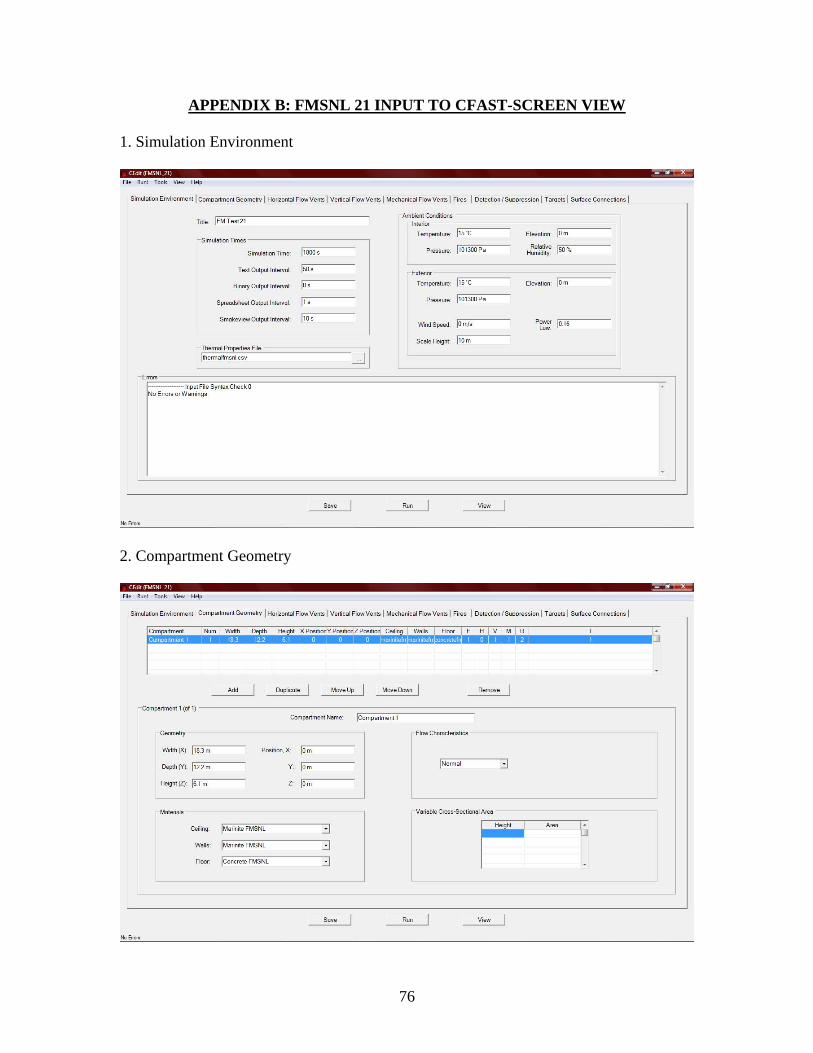
76
APPENDIX B: FMSNL 21 INPUT TO CFAST-SCREEN VIEW 1. Simulation Environment
2. Compartment Geometry
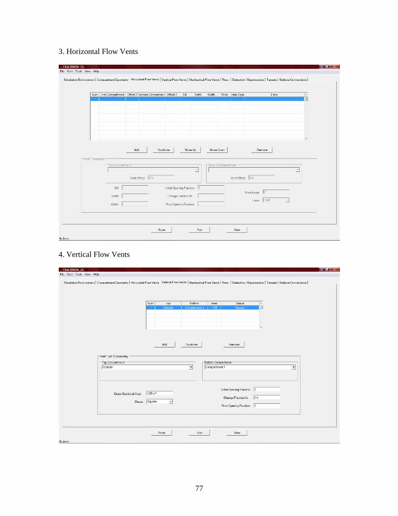
77
3. Horizontal Flow Vents
4. Vertical Flow Vents
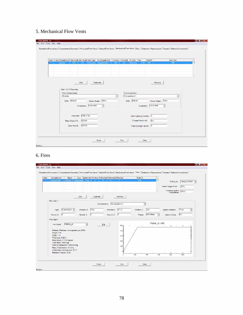
78
5. Mechanical Flow Vents
6. Fires
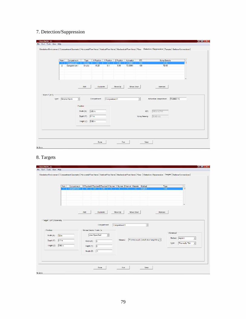
79
7. Detection/Suppression
8. Targets
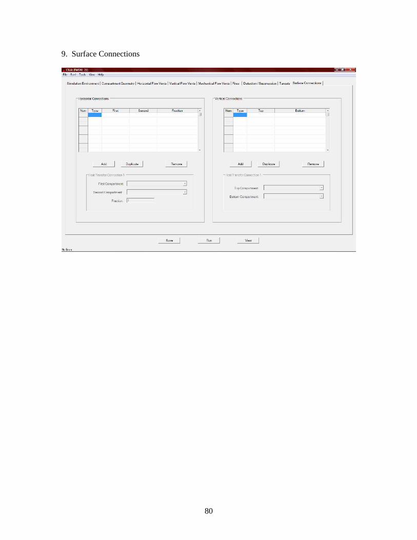
80
9. Surface Connections
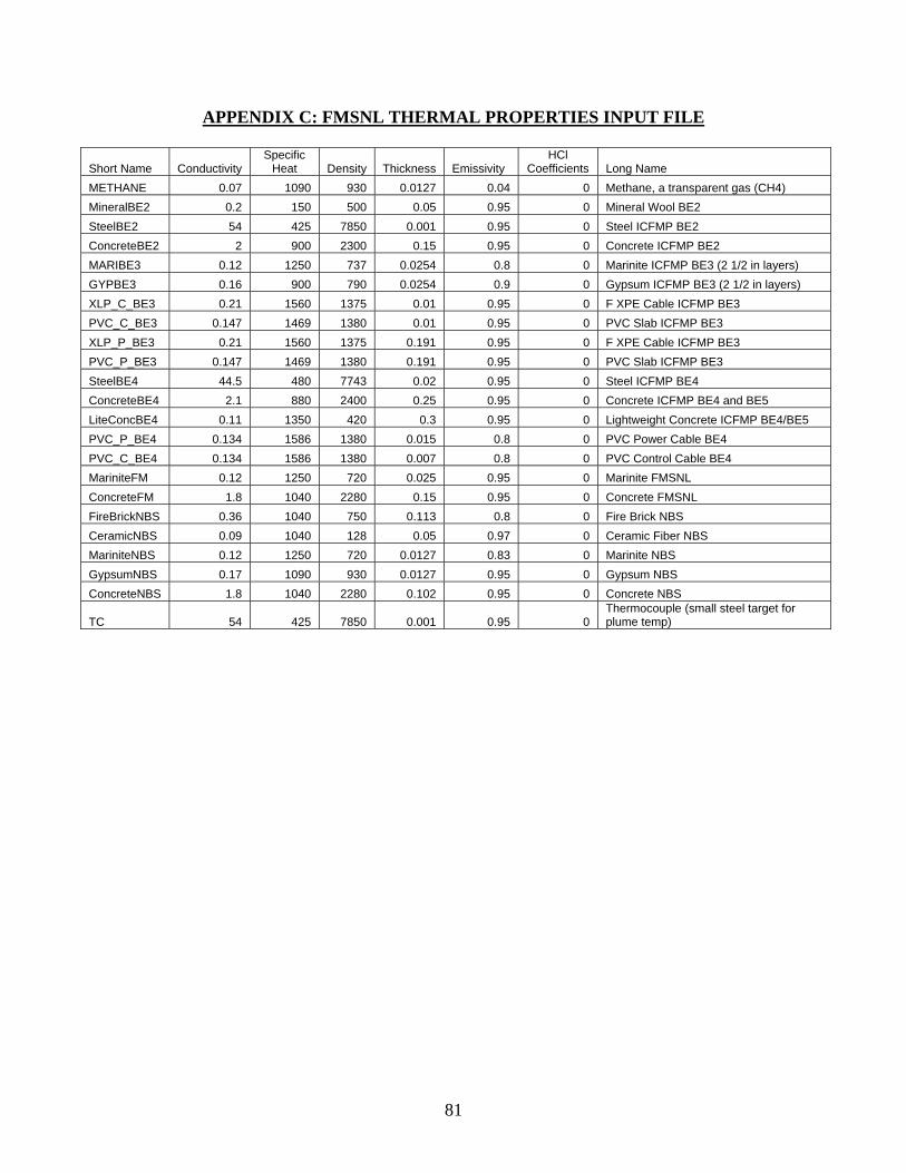
81
APPENDIX C: FMSNL THERMAL PROPERTIES INPUT FILE
Short Name Conductivity Specific
Heat Density Thickness Emissivity HCl
Coefficients Long Name METHANE 0.07 1090 930 0.0127 0.04 0 Methane, a transparent gas (CH4) MineralBE2 0.2 150 500 0.05 0.95 0 Mineral Wool BE2 SteelBE2 54 425 7850 0.001 0.95 0 Steel ICFMP BE2 ConcreteBE2 2 900 2300 0.15 0.95 0 Concrete ICFMP BE2 MARIBE3 0.12 1250 737 0.0254 0.8 0 Marinite ICFMP BE3 (2 1/2 in layers) GYPBE3 0.16 900 790 0.0254 0.9 0 Gypsum ICFMP BE3 (2 1/2 in layers) XLP_C_BE3 0.21 1560 1375 0.01 0.95 0 F XPE Cable ICFMP BE3 PVC_C_BE3 0.147 1469 1380 0.01 0.95 0 PVC Slab ICFMP BE3 XLP_P_BE3 0.21 1560 1375 0.191 0.95 0 F XPE Cable ICFMP BE3 PVC_P_BE3 0.147 1469 1380 0.191 0.95 0 PVC Slab ICFMP BE3 SteelBE4 44.5 480 7743 0.02 0.95 0 Steel ICFMP BE4 ConcreteBE4 2.1 880 2400 0.25 0.95 0 Concrete ICFMP BE4 and BE5 LiteConcBE4 0.11 1350 420 0.3 0.95 0 Lightweight Concrete ICFMP BE4/BE5 PVC_P_BE4 0.134 1586 1380 0.015 0.8 0 PVC Power Cable BE4 PVC_C_BE4 0.134 1586 1380 0.007 0.8 0 PVC Control Cable BE4 MariniteFM 0.12 1250 720 0.025 0.95 0 Marinite FMSNL ConcreteFM 1.8 1040 2280 0.15 0.95 0 Concrete FMSNL FireBrickNBS 0.36 1040 750 0.113 0.8 0 Fire Brick NBS CeramicNBS 0.09 1040 128 0.05 0.97 0 Ceramic Fiber NBS MariniteNBS 0.12 1250 720 0.0127 0.83 0 Marinite NBS GypsumNBS 0.17 1090 930 0.0127 0.95 0 Gypsum NBS ConcreteNBS 1.8 1040 2280 0.102 0.95 0 Concrete NBS
TC 54 425 7850 0.001 0.95 0 Thermocouple (small steel target for plume temp)
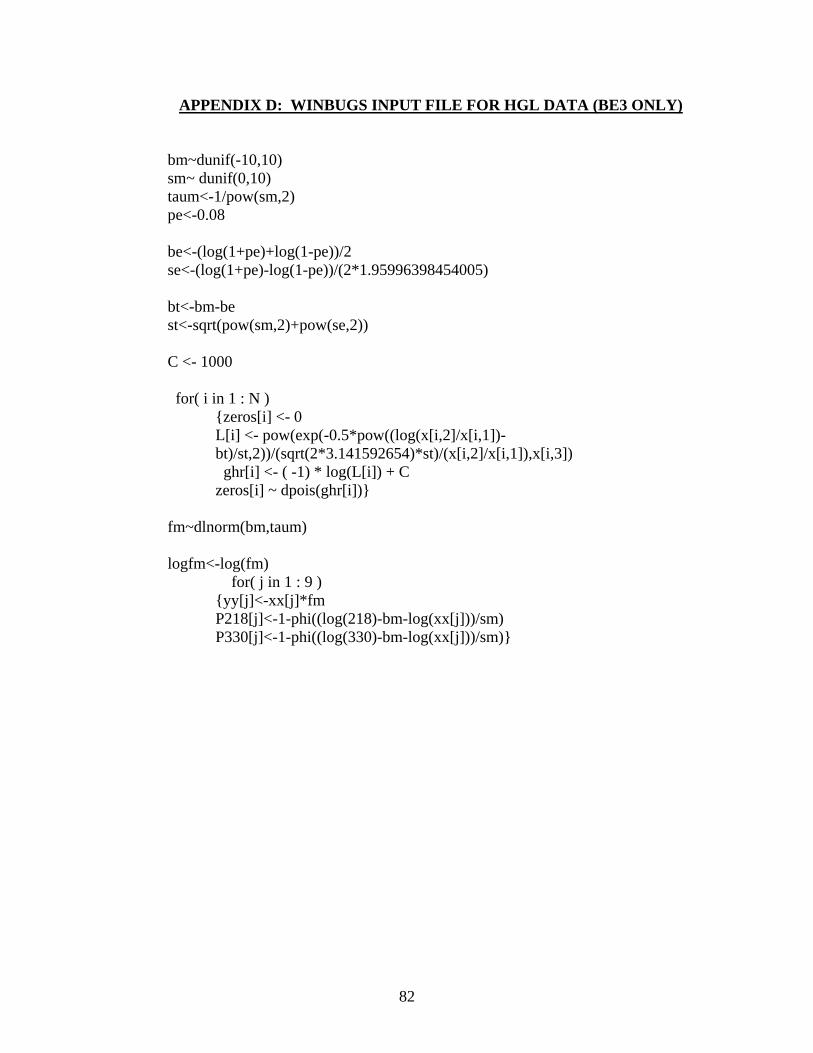
82
APPENDIX D: WINBUGS INPUT FILE FOR HGL DATA (BE3 ONLY) bm~dunif(-10,10) sm~ dunif(0,10) taum<-1/pow(sm,2) pe<-0.08 be<-(log(1+pe)+log(1-pe))/2 se<-(log(1+pe)-log(1-pe))/(2*1.95996398454005) bt<-bm-be st<-sqrt(pow(sm,2)+pow(se,2)) C <- 1000 for( i in 1 : N ) {zeros[i] <- 0 L[i] <- pow(exp(-0.5*pow((log(x[i,2]/x[i,1])- bt)/st,2))/(sqrt(2*3.141592654)*st)/(x[i,2]/x[i,1]),x[i,3]) ghr[i] <- ( -1) * log(L[i]) + C zeros[i] ~ dpois(ghr[i])} fm~dlnorm(bm,taum) logfm<-log(fm) for( j in 1 : 9 ) {yy[j]<-xx[j]*fm P218[j]<-1-phi((log(218)-bm-log(xx[j]))/sm) P330[j]<-1-phi((log(330)-bm-log(xx[j]))/sm)}
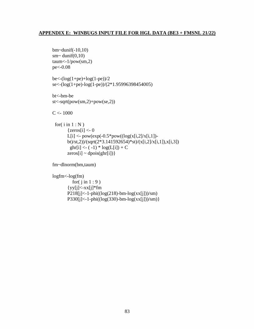
83
APPENDIX E: WINBUGS INPUT FILE FOR HGL DATA (BE3 + FMSNL 21/22) bm~dunif(-10,10) sm~ dunif(0,10) taum<-1/pow(sm,2) pe<-0.08 be<-(log(1+pe)+log(1-pe))/2 se<-(log(1+pe)-log(1-pe))/(2*1.95996398454005) bt<-bm-be st<-sqrt(pow(sm,2)+pow(se,2)) C <- 1000 for( i in 1 : N ) {zeros[i] <- 0 L[i] <- pow(exp(-0.5*pow((log(x[i,2]/x[i,1])- bt)/st,2))/(sqrt(2*3.141592654)*st)/(x[i,2]/x[i,1]),x[i,3]) ghr[i] <- ( -1) * log(L[i]) + C zeros[i] ~ dpois(ghr[i])} fm~dlnorm(bm,taum) logfm<-log(fm) for( j in 1 : 9 ) {yy[j]<-xx[j]*fm P218[j]<-1-phi((log(218)-bm-log(xx[j]))/sm) P330[j]<-1-phi((log(330)-bm-log(xx[j]))/sm)}
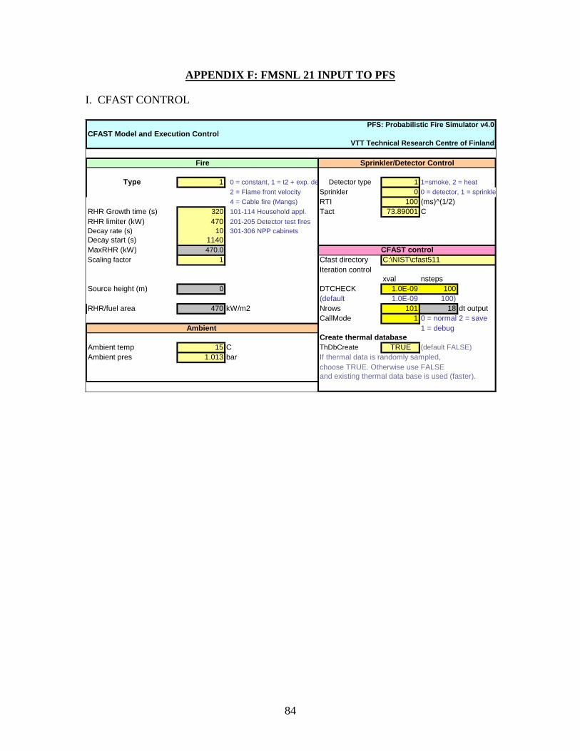
84
APPENDIX F: FMSNL 21 INPUT TO PFS I. CFAST CONTROL
PFS: Probabilistic Fire Simulator v4.0CFAST Model and Execution Control
VTT Technical Research Centre of Finland
Type 1 0 = constant, 1 = t2 + exp. de Detector type 1 1=smoke, 2 = heat 2 = Flame front velocity Sprinkler 0 0 = detector, 1 = sprinkle 4 = Cable fire (Mangs) RTI 100 (ms)^(1/2)
RHR Growth time (s) 320 101-114 Household appl. Tact 73.89001 CRHR limiter (kW) 470 201-205 Detector test firesDecay rate (s) 10 301-306 NPP cabinetsDecay start (s) 1140MaxRHR (kW) 470.0Scaling factor 1 Cfast directory
Iteration controlxval nsteps
Source height (m) 0 DTCHECK 1.0E-09 100(default 1.0E-09 100)
RHR/fuel area 470 kW/m2 Nrows 101 18 dt outputCallMode 1 0 = normal 2 = save
1 = debugCreate thermal database
Ambient temp 15 C ThDbCreate TRUE (default FALSE)Ambient pres 1.013 bar If thermal data is randomly sampled,
choose TRUE. Otherwise use FALSEand existing thermal data base is used (faster).
Sprinkler/Detector Control
Ambient
Fire
CFAST controlC:\NIST\cfast511
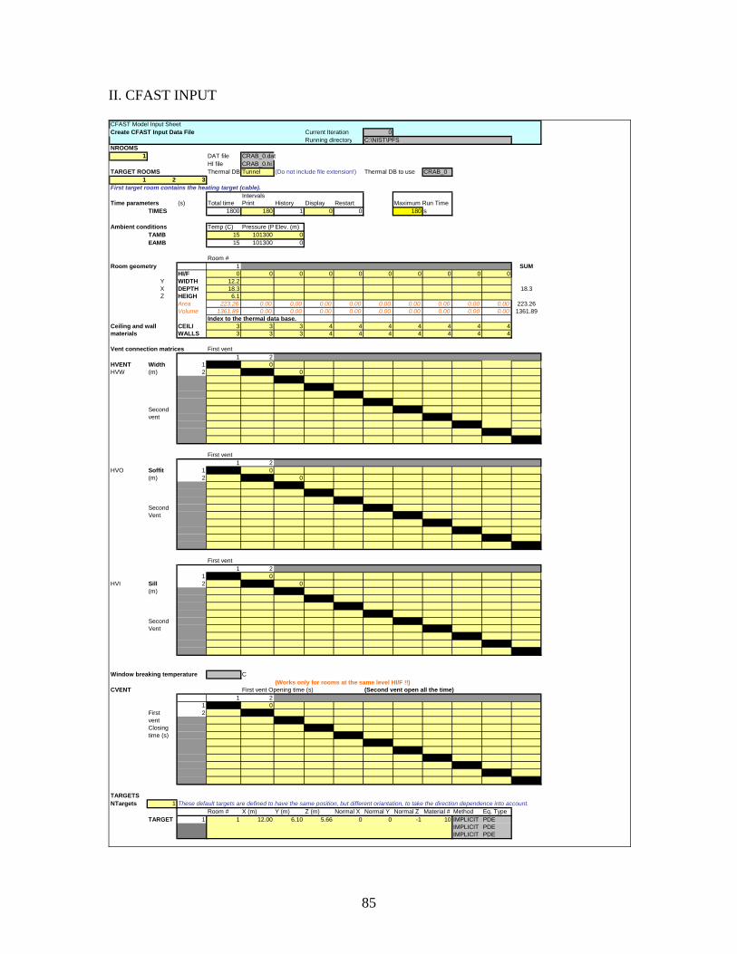
85
II. CFAST INPUT CFAST Model Input SheetCreate CFAST Input Data File Current Iteration 0
Running directoryNROOMS
1 DAT file CRAB_0.datHI file CRAB_0.hi
TARGET ROOMS Thermal DB Tunnel (Do not include file extension!) Thermal DB to use CRAB_01 2 3
First target room contains the heating target (cable).Intervals
Time parameters (s) Total time Print History Display Restart Maximum Run TimeTIMES 1800 180 1 0 0 180 s
Ambient conditions Temp (C) Pressure (P Elev. (m)TAMB 15 101300 0EAMB 15 101300 0
Room #Room geometry 1 2 3 4 5 6 7 8 9 10 SUM
HI/F 0 0 0 0 0 0 0 0 0 0Y WIDTH 12.2X DEPTH 18.3 18.3Z HEIGH 6.1
Area 223.26 0.00 0.00 0.00 0.00 0.00 0.00 0.00 0.00 0.00 223.26Volume 1361.89 0.00 0.00 0.00 0.00 0.00 0.00 0.00 0.00 0.00 1361.89
Index to the thermal data base.Ceiling and wall CEILI 3 3 3 4 4 4 4 4 4 4materials WALLS 3 3 3 4 4 4 4 4 4 4
Vent connection matrices First vent1 2 3 4 5 6 7 8 9 10 11
HVENT Width 1 0HVW (m) 2 0
3456
Second 7vent 8
91011
First vent1 2 3 4 5 6 7 8 9 10 11
HVO Soffit 1 0(m) 2 0
345
Second 6Vent 7
89
1011
First vent1 2 3 4 5 6 7 8 9 10 11
1 0HVI Sill 2 0
(m) 3456
Second 7Vent 8
91011
Window breaking temperature C(Works only for rooms at the same level HI/F !!)
CVENT First vent Opening time (s) (Second vent open all the time)1 2 3 4 5 6 7 8 9 10 11
1 0First 2vent 3Closing 4time (s) 5
6789
1011
TARGETSNTargets 1 These default targets are defined to have the same position, but different oriantation, to take the direction dependence into account.
Room # X (m) Y (m) Z (m) Normal X Normal Y Normal Z Material # Method Eq. TypeTARGET 1 1 12.00 6.10 5.66 0 0 -1 10 IMPLICIT PDE
2 IMPLICIT PDE3 IMPLICIT PDE
C:\NIST\PFS
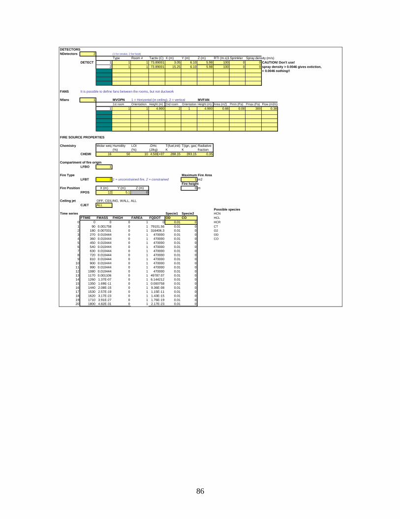
86
DETECTORSNDetectors 2 (1 for smoke, 2 for heat)
Type Room # Tactiv (C) X (m) Y (m) Z (m) RTI (m.s)1Sprinkler Spray density (m/s)DETECT 1 1 1 73.89001 3.05 6.10 5.98 100 0 0 CAUTION! Don't use!
2 1 1 73.89001 15.25 6.10 5.98 100 0 0 spray density > 0.0046 gives extiction,3 < 0.0046 nothing!!456
FANS It is possible to define fans between the rooms, but not ductwork
Nfans 1 MVOPN 1 = Horizontal (in ceiling), 2 = vertical MVFAN1st room Orientatiion Height (m) 2nd room Orientation Height (m) Area (m2) Pmin (Pa) Pmax (Pa) Flow (m3/s)
1 1 1 4.900 2 1 4.900 0.66 0.00 300 0.3823456
FIRE SOURCE PROPERTIES
Chemistry Molar weigHumidity LOI -DHc T(fuel,init) T(ign, gas)Radiative(%) (%) (J/kg) K K fraction
CHEMI 16 50 10 4.50E+07 288.15 393.15 0.35
Compartment of fire originLFBO 1
Fire Type Maximum Fire AreaLFBT 2 1 = unconstrained fire, 2 = constrained 1 m2
Fire heightFire Position X (m) Y (m) Z (m) 0 m
FPOS 12 5.1 0
Ceiling jet OFF, CEILING, WALL, ALLCJET ALL
Possible speciesTime series Specie1 Specie2 HCN
FTIME FMASS FHIGH FAREA FQDOT OD CO HCL0 0 0 0 1 0 0.01 0 HCR1 90 0.001758 0 1 79101.56 0.01 0 CT2 180 0.007031 0 1 316406.3 0.01 0 O23 270 0.010444 0 1 470000 0.01 0 OD4 360 0.010444 0 1 470000 0.01 0 CO5 450 0.010444 0 1 470000 0.01 06 540 0.010444 0 1 470000 0.01 07 630 0.010444 0 1 470000 0.01 08 720 0.010444 0 1 470000 0.01 09 810 0.010444 0 1 470000 0.01 0
10 900 0.010444 0 1 470000 0.01 011 990 0.010444 0 1 470000 0.01 012 1080 0.010444 0 1 470000 0.01 013 1170 0.001106 0 1 49787.07 0.01 014 1260 1.37E-07 0 1 6.144212 0.01 015 1350 1.69E-11 0 1 0.000758 0.01 016 1440 2.08E-15 0 1 9.36E-08 0.01 017 1530 2.57E-19 0 1 1.15E-11 0.01 018 1620 3.17E-23 0 1 1.43E-15 0.01 019 1710 3.91E-27 0 1 1.76E-19 0.01 020 1800 4.82E-31 0 1 2.17E-23 0.01 0

87
APPENDIX G: STUDENT BIOGRAPHY
Lieutenant Mark Minton is originally from Northern California and enlisted in the
United States Navy after graduating from Clayton Valley High School in 1995. After
completing the Naval Nuclear Power School enlisted curriculum, he was selected for the
Nuclear Enlisted Commissioning Program and ordered to Oregon State University, where
he received a Bachelor of Science in Nuclear Engineering in 2001.
After being commissioned, he reported to USS SHOUP (DDG 86), where he
served as Communications Officer and achieved qualification as a Surface Warfare
Officer. He was subsequently ordered to return to Naval Nuclear Power School, this time
to complete the officer curriculum.
Upon completion of Nuclear Power training, Lieutenant Minton reported to USS
RONALD REAGAN (CVN 76) where he served in Reactor Department and achieved
qualification as Nuclear Engineering Officer. He was subsequently selected for lateral
transfer to the Engineering Duty Officer (Nuclear) community.
In 2008, Lieutenant Minton received a Master of Engineering Management from
Old Dominion University.
Lieutenant Minton is currently pursuing a Nuclear Engineer’s Degree and a
Master of Science in Nuclear Science in Engineering at the Massachusetts Institute of
Technology.
Upon completion of his studies at the Massachusetts Institute of Technology,
Lieutenant Minton has been ordered to report to the Supervisor of Shipbuilding, Newport
News, Virginia, where he will be assigned duties pertaining to the design, construction,
conversion, and overhaul of nuclear powered aircraft carriers.