missie aguado-rojas, william pasillas-lépine, antonio loria

HAL Id: hal-02367580https://hal.archives-ouvertes.fr/hal-02367580

Submitted on 5 Mar 2020

HAL is a multi-disciplinary open accessarchive for the deposit and dissemination of sci-entific research documents, whether they are pub-lished or not. The documents may come fromteaching and research institutions in France orabroad, or from public or private research centers.

L’archive ouverte pluridisciplinaire HAL, estdestinée au dépôt et à la diffusion de documentsscientifiques de niveau recherche, publiés ou non,émanant des établissements d’enseignement et derecherche français ou étrangers, des laboratoirespublics ou privés.

A hybrid controller for ABS based onextended-braking-stiffness estimation

Missie Aguado-Rojas, William Pasillas-Lépine, Antonio Loria

To cite this version:Missie Aguado-Rojas, William Pasillas-Lépine, Antonio Loria. A hybrid controller for ABS basedon extended-braking-stiffness estimation. IFAC-PapersOnLine, Elsevier, 2019, 9th IFAC Symposiumon Advances in Automotive Control AAC 2019, 52 (5), pp.452-457. �10.1016/j.ifacol.2019.09.072�.�hal-02367580�

https://hal.archives-ouvertes.fr/hal-02367580

https://hal.archives-ouvertes.fr

A hybrid controller for ABS based onextended-braking-stiffness estimation ?

Missie Aguado-Rojas ∗ William Pasillas-Lepine ∗∗ Antonio Lorıa ∗∗

∗Universite Paris-Sud, Universite Paris-Saclay,L2S-CentraleSupelec, 91192 Gif-sur-Yvette, France

∗∗ CNRS, L2S-CentraleSupelec, 91192 Gif-sur-Yvette, France(e-mails: {missie.aguado}{pasillas}{loria}@l2s.centralesupelec.fr)

Abstract: In the context of antilock braking systems (ABS), we present a two-phase hybridcontrol algorithm based on the tyre extended braking stiffness (XBS), that is, on the slope of thetyre-road friction coefficient with respect to the wheel slip. Because the XBS cannot be directlymeasured, a switched observer is used to estimate it. With the proposed hybrid algorithm,the closed-loop trajectories of the system satisfy the conditions required for the observer tocorrectly estimate the XBS. Moreover, the braking distances are shorter than those obtainedusing a hybrid algorithm based on wheel deceleration thresholds.

Keywords: ABS; braking distance; switched systems; persistency of excitation;

1. INTRODUCTION

Introduced by Bosch in 1978 for production passengercars, the antilock braking system (ABS) is the core oftoday’s active driving-safety systems. Its main objectivesare to prevent the wheels from locking in order to maintainthe stability and steerability of the vehicle during heavybraking, and to maximally exploit the tyre-road frictioncoefficient in order to achieve the shortest possible brakingdistance [Corno et al., 2012; Singh et al., 2013].

Most commercial ABS use a regulation logic basedon wheel deceleration thresholds (see, e.g. Kiencke andNielsen [2005]; Gerard et al. [2012]; Reif [2014]). Theprinciple of these algorithms is based on generating limitcycles in a desired range of longitudinal wheel slip. Themain force of these controllers is that they are able to keepwheel slip in a neighborhood of the optimal point withoutusing explicitly its value and they are quite robust withrespect to changes in tyre parameters and road conditions.Their main drawback, however, is that they are oftenbased on purely heuristic arguments and the tuning of thedeceleration thresholds is not an easy task [Choi, 2008;Hoang et al., 2014]. Moreover, the wheel-slip cycling rangecannot be explicitly chosen; instead, it has to be selectedindirectly through the wheel deceleration thresholds. Theobjective of this paper is to design an algorithm that allowsthe cycling range to be chosen in a more direct manner.To that end, we present a regulation logic based on thetyre extended braking stiffness (XBS).

The braking stiffness is the slope of the tyre-road frictioncurve with respect to the wheel slip at the zero-frictionoperating point [Gustafsson, 1997]. As a generalization ofthis concept, the XBS may be defined as the slope of thefriction-vs-slip curve at any operating point [Sugai et al.,1999; Umeno, 2002]. The interest of using the XBS is that,

? The work of the first author is supported by CONACYT, Mexico.

in contrast to the unknown optimal value of wheel slip, theoptimal value of XBS is always known and equal to zero.Hence, the (control) objective of an ABS algorithm maybe reformulated in terms of this variable. In other words,our objective is to design an algorithm such that the XBSremains in a neighbourhood around zero.

The concept of maximizing the braking force in an ABSbased on the XBS was introduced by Sugai et al. [1999],and was later extended by Umeno [2002] and Ono et al.[2003]. In these works, however, the XBS is implicitlyassumed to be a constant parameter so its dynamics isneglected. In Villagra et al. [2011], in order to estimatethe maximum friction coefficient, the XBS is used to signalthe entrance of the tyre into a different road surface andto distinguish one type of road from another. In Hoanget al. [2014] the XBS is used to perform closed-loop wheelacceleration control during some phases of a five-phasewheel-deceleration-based algorithm.

In this paper, a two-phase algorithm based on XBS thresh-olds is developed. This work builds upon the results pre-sented in Aguado-Rojas et al. [2018], where an observerto estimate the XBS under unknown road conditionswas introduced. By directly choosing the values of XBSthresholds, the proposed algorithm allows an easier andmore direct selection of the wheel-slip cycling range and,consequently, to reduce the braking distance. Moreover,it is shown that the trajectories of the system satisfy theconditions required for the observer to correctly estimatethe XBS, which may not be achieved with continuouscontrol algorithms.

2. XBS DYNAMICS

Consider a quarter-car model composed of a wheel withradius R and angular velocity ω mounted on a vehicle withlongitudinal velocity vx. The normalized relative velocitybetween the vehicle and the tyre, known as the wheel slip

0

XBS

Wheel slip0-1 1

Braking Traction

Stable regionof the tyre

Unstable region

Optimalpoint

Fig. 1. Typical shape of the XBS-vs-slip curve.

λ =(Rω − vx

)/vx,

determines the friction coefficient µ between the tyre andthe road through a nonlinear relation µ(λ).

Define as state variables the wheel acceleration offset

z1 := Rω − vx(t),

that is, the difference between the longitudinal accelerationof the vehicle and the linear acceleration of the tyre at thewheel-ground contact point, and

z2 := µ′(λ),

that is, the tyre extended braking stiffness (XBS). Theshape of the curve µ′(λ) is illustrated in Fig. 1. The pointat which the maximum braking force can be obtainedcorresponds to z2 = 0. The area above this point iscalled the stable region of the tyre, and the area belowis called the unstable region. Given a suitable choice forthe tyre-road friction µ(λ), a simple second-order modelin which the XBS appears directly as a state variable canbe developed. In this work the friction model proposed byBurckhardt [1993] is used, hence the XBS is modelled as

µ′(λ) = c1c2 exp(−c2λ)− c3,where the coefficients ci are constants that depend on theroad conditions.

During an ABS braking scenario, vx(t) remains almostconstant and close to the maximal value allowed by theroad conditions, while λ remains relatively small. Undersuch conditions, the dynamics of z1 and z2 are describedby 1

z1 = − a

vx(t)z1z2 − bu (1a)

z2 =(cz2 + d

) z1vx(t)

(1b)

y = z1, (1c)

where the control input u is the derivative of the brakepressure, the measured output y is the wheel accelerationoffset, the positive parameters a and b depend on thegeometrical characteristics of the wheel, and c and d onthe road conditions. All parameters are assumed to beknown and constant. The vehicle speed vx(t) is consideredas a known external variable and assumed to be positive,bounded, and bounded away from zero.

The aim of this paper is to design a control law suchthat the XBS remains close to its optimal value and thusmaximize the braking force during an emergency brakingscenario.1 See Hoang et al. [2014] and Aguado-Rojas et al. [2018] for thecomplete derivation of this model.

3. CONTINUOUS CONTROL DESIGN

To simplify the control design, let us assume for themoment that both z1 and z2 are known. Under thisassumption, one may design a control law that stabilizessystem (1) at the origin. Note, however, that because thecontrol input u does not appear explicitly in (1b), onemust achieve the objective through z1, that is, regardingthe latter as a virtual control.

Hence, we first design a virtual reference z∗1 such that ifz1 = z∗1 , then z2 → z∗2 = 0. One such reference is

z∗1 = −krz2

cz2 + d, kr > 0, (2)

since, setting z1 = z∗1 in (1b) leads to z2 = −krz2/vx(t)which is exponentially stable.

To perform the tracking of z∗1 , the control is designed as

u =1

b

[− a

vx(t)z1z2 +

kpvx(t)

(z1 − z∗1

)− z∗1

], kp > 0,

(3)where we employ (1b) in the evaluation of z∗1 . Hence, thelatter is implemented using z1 and z2 as

z∗1 = − krvx(t)

dz1cz2 + d

.

Note that, even though the right-hand side of (2) is notdefined when z2 = −d/c, this singularity lies outside thedomain in which z2 is physically feasible. Indeed, thereexist zmax

2 ≥ z2 ≥ zmin2 > −d/c. Hence, z∗1 is well-posed.

Now, let z1 := z1 − z∗1 and z2 = z2 − z∗2 . Substitution of(3) in (1a) yields the closed-loop dynamics

z1 =kpvx(t)

(z∗1 − z1

)+ z∗1 = − kp

vx(t)z1 + z∗1

and from (1b) and (2) one has

z2 =(cz2 + d

) z∗1vx(t)

+(cz2 + d

) z1vx(t)

= − krvx(t)

z2 +(cz2 + d

) z1vx(t)

.

Hence, the tracking error dynamics is

˙z1 = − kpvx(t)

z1 (4a)

˙z2 = − krvx(t)

z2 +cz2 + d

vx(t)z1, (4b)

which has a cascaded structure. This is relevant because,for cascaded systems, sufficient conditions for the originto be globally asymptotically stable (GAS) are well es-tablished. It is enough that the origin for (4a) be GAS,that the origin for (4b) with z1 = 0 be GAS, and that thesolutions of (4) be uniformly globally bounded [Panteleyand Lorıa, 2001].

Now, recalling that vx(t) is positive, bounded, andbounded away from zero, it follows that the origin of (4a)is GAS. The same holds for the origin of

˙z2 = − krvx(t)

z2.

Moreover, note that because z∗2 = 0, the tracking errorz2 = z2 is the XBS itself, which is bounded by nature.Thus, the interconnection term

(cz2 +d

)/vx(t) is bounded

and so are the solutions of (4). Therefore, it follows by acascade argument that the origin of (4) is GAS.

-0.8 -0.6 -0.4 -0.2 0 0.2 0.4-10

-8

-6

-4

-2

0

2

4

-0.8 -0.6 -0.4 -0.2 0 0.2 0.4-60

-45

-30

-15

0

15

30

45

Fig. 2. Continuous state-feedback control: the system converges to the origin. Left: The estimated states do notconverge to their true values because z1 → 0 (hence, it is not persistently exciting). Right: During the transientstage, the estimate z2 crosses the set {cz2 + d = 0}.

-0.8 -0.6 -0.4 -0.2 0 0.2 0.4-10

-8

-6

-4

-2

0

2

4

-0.8 -0.6 -0.4 -0.2 0 0.2 0.4-60

-45

-30

-15

0

15

30

45

Fig. 3. Continuous output-feedback control using XBS observer: z2 does not converge to its optimal value. Left: Theestimated states do not converge to their true values because z1 → 0 (hence, it is not persistently exciting). Right:Even though the true trajectories of the system remain within the feasible region, as z2 approaches −d/c, thedenominator of the right-hand side of (2) approaches zero and z∗1 grows unbounded. The simulation is stoppedwhen a division by zero is detected.

The performance of this control law is illustrated in Fig. 2.Unless otherwise stated, in what follows we consider a sim-ulation scenario of a vehicle braking on dry asphalt with aninitial speed of 90 km/h. The graphics show the evolutionof the system (solid line, blue) on the phase-plane fortwo different initial conditions (the trajectories labeled‘observer’ will be discussed later on). Not surprisingly, thecontrol law given by (2) and (3) is able to smoothly steerthe system’s trajectories towards the origin. We recall,however, that we have momentarily assumed that z1 andz2 are known, but in a real-time implementation z2 cannotbe directly measured. Hence, in order to implement thecontrol law, an estimate z2 must be used instead. Togenerate such an estimate, an observer is presented in thefollowing section.

4. XBS OBSERVER

Under the assumptions established in Section 2, an ob-server for system (1) may be designed as

˙z1 = − a

vx(t)z1z2 − bu+ k1(z1)

z1vx(t)

(z1 − z1

)(5a)

˙z2 =(cz2 + d

) z1vx(t)

+ k2(z1)z1vx(t)

(z1 − z1

), (5b)

where

ki(z1) =

{k+i if z1 > 0

k−i if z1 < 0for i = {1, 2}. (6)

Define the estimation errors z1 := z1−z1 and z2 := z2−z2.From (1) and (5), one has[

˙z1˙z2

]=

z1vx(t)

[−k1(z1) −a−k2(z1) c

] [z1z2

]. (7)

The observer described by (5) and (6) is a particular caseof those presented in Hoang et al. [2014] and Aguado-Rojaset al. [2018] (in this work the road parameters c and d areassumed to be known, but in the aforementioned referencessuch is not the case). It is a Luenberger-like observer inwhich the gains ki(z1) switch between two different valuesk+i and k−i depending on the sign of z1. Following the sameapproach used in those references, it can be shown that ifthe gains k+i and k−i satisfy

k+1 > c, k+2 < − cak+1 , k−1 < c, k−2 < − c

ak−1 ,

k−1 = 2c− k+1 , ck+1 + ak+2 = ck−1 + ak−2 ,(8)

then the origin of (7) is asymptotically stable, providedthat: (i) z1 is persistently exciting (PE), (ii) z1 crosses zeroonly at isolated points, and (iii) any two such points areseparated by an interval of length no smaller than τD > 0.

The condition (i) holds if there exist positive constants µ0

and T0 such that∫ t+T0

t

z1(ς)2dς ≥ µ0 for all t ≥ 0. (9)

Roughly speaking, (9) means that z1 should be rich enoughto guarantee that the solutions of (7) do not become tooslow or remain “stuck” away from zero. The condition (ii)renders the system observable even when it crosses theset {z1 = 0} on which the system is not observable. Theconditions (ii) and (iii) imply that there exists a minimaldwell time τD > 0 between each consecutive switch of thegains k+i and k−i . This three conditions, together with (8),guarantee the asymptotic stability of (7) [Aguado-Rojaset al., 2018].

Fig. 3 illustrates the performance of the control law ofSection 3 when (2) and (3) are implemented using z2instead of z2. In both cases the control fails to drive thesystem towards the origin. This is caused by two problems:(a) the control law does not guarantee that z1 is PEbecause z1 → 0, and (b) the observer does not guaranteethat z2 remains within a feasible region for all t. Consideragain Fig. 2-Left. The graphic shows the evolution of theobserver (dash-dotted line, green) when it is implementedin open loop (that is, independently from the control).In this case, the trajectory of z1 does not satisfy thepersistency of excitation condition so the estimated statesdo not converge to their true values. When the controlis implemented in closed loop with the observer (Fig. 3-Left), this causes the system to converge to a pointdifferent than the origin. Now, consider Fig. 2-Right. Inthis case the estimated states do converge to the truetrajectory of the system. However, during the transientstage z2 crosses into a region in which such a value ofz2 is not feasible. When the control is implemented inclosed-loop with the observer (Fig. 3-Right), the referencez∗1 grows unbounded as z2 approaches −d/c. When z2crosses the set {cz2 + d = 0} (dashed line, red), z∗1 andconsequently u are no longer defined. To circumvent theseproblems, in the following section we redefine the virtualreference z∗1 such that (9) is satisfied.

5. HYBRID CONTROL DESIGN

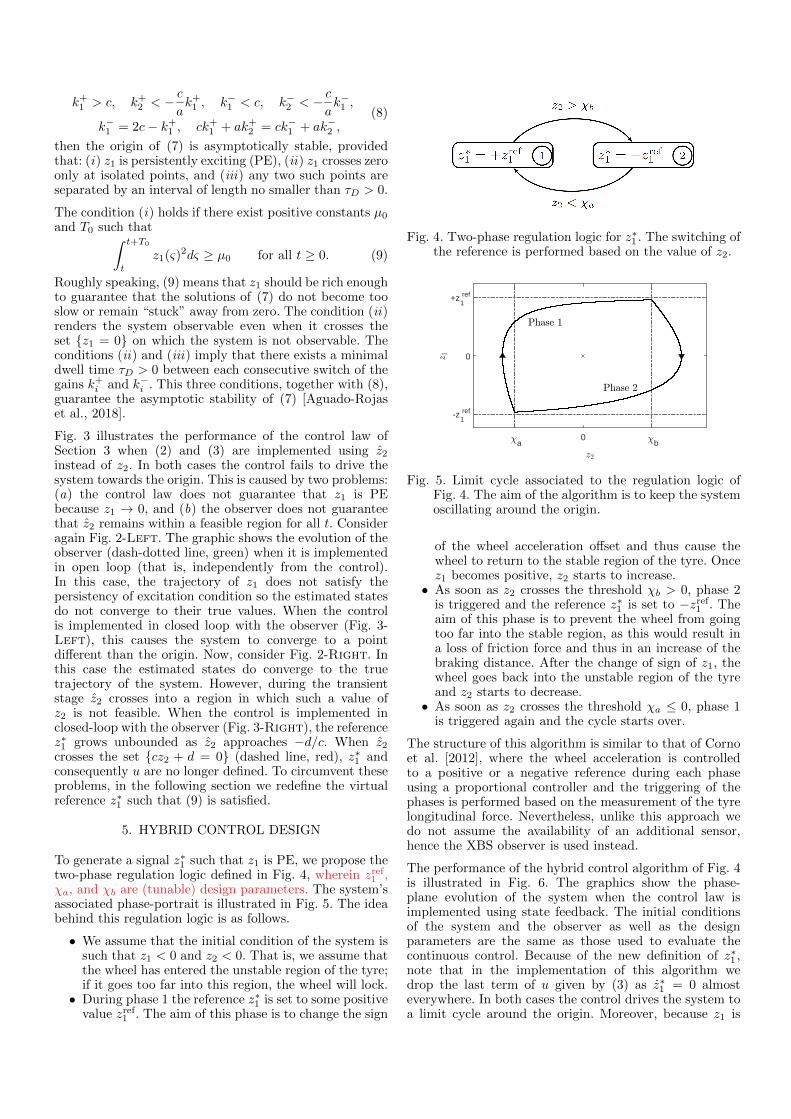
To generate a signal z∗1 such that z1 is PE, we propose thetwo-phase regulation logic defined in Fig. 4, wherein zref1 ,χa, and χb are (tunable) design parameters. The system’sassociated phase-portrait is illustrated in Fig. 5. The ideabehind this regulation logic is as follows.

• We assume that the initial condition of the system issuch that z1 < 0 and z2 < 0. That is, we assume thatthe wheel has entered the unstable region of the tyre;if it goes too far into this region, the wheel will lock.• During phase 1 the reference z∗1 is set to some positive

value zref1 . The aim of this phase is to change the sign

Fig. 4. Two-phase regulation logic for z∗1 . The switching ofthe reference is performed based on the value of z2.

a0 b

-z1 ref

0

+z1 ref

Fig. 5. Limit cycle associated to the regulation logic ofFig. 4. The aim of the algorithm is to keep the systemoscillating around the origin.

of the wheel acceleration offset and thus cause thewheel to return to the stable region of the tyre. Oncez1 becomes positive, z2 starts to increase.

• As soon as z2 crosses the threshold χb > 0, phase 2is triggered and the reference z∗1 is set to −zref1 . Theaim of this phase is to prevent the wheel from goingtoo far into the stable region, as this would result ina loss of friction force and thus in an increase of thebraking distance. After the change of sign of z1, thewheel goes back into the unstable region of the tyreand z2 starts to decrease.

• As soon as z2 crosses the threshold χa ≤ 0, phase 1is triggered again and the cycle starts over.

The structure of this algorithm is similar to that of Cornoet al. [2012], where the wheel acceleration is controlledto a positive or a negative reference during each phaseusing a proportional controller and the triggering of thephases is performed based on the measurement of the tyrelongitudinal force. Nevertheless, unlike this approach wedo not assume the availability of an additional sensor,hence the XBS observer is used instead.

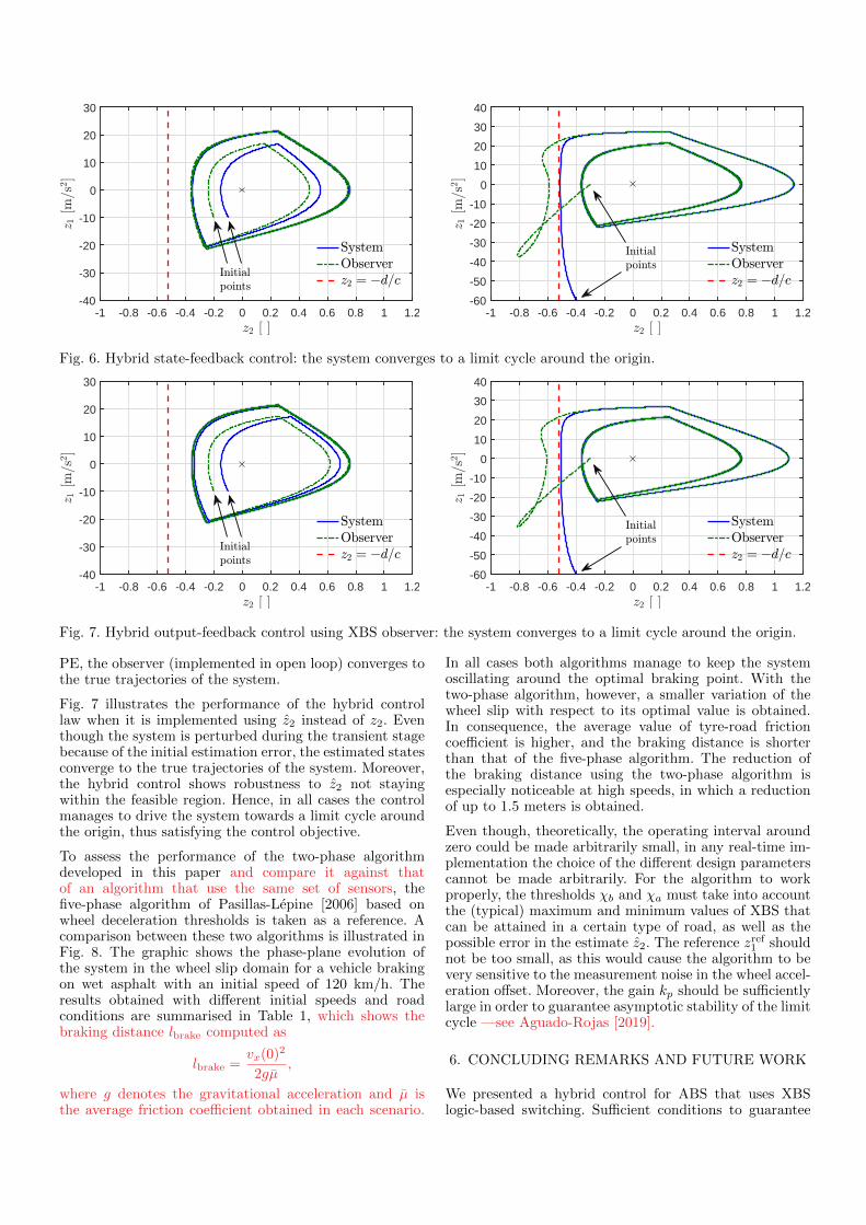
The performance of the hybrid control algorithm of Fig. 4is illustrated in Fig. 6. The graphics show the phase-plane evolution of the system when the control law isimplemented using state feedback. The initial conditionsof the system and the observer as well as the designparameters are the same as those used to evaluate thecontinuous control. Because of the new definition of z∗1 ,note that in the implementation of this algorithm wedrop the last term of u given by (3) as z∗1 = 0 almosteverywhere. In both cases the control drives the system toa limit cycle around the origin. Moreover, because z1 is

-1 -0.8 -0.6 -0.4 -0.2 0 0.2 0.4 0.6 0.8 1 1.2-40

-30

-20

-10

0

10

20

30

-1 -0.8 -0.6 -0.4 -0.2 0 0.2 0.4 0.6 0.8 1 1.2-60

-50

-40

-30

-20

-10

0

10

20

30

40

Fig. 6. Hybrid state-feedback control: the system converges to a limit cycle around the origin.

-1 -0.8 -0.6 -0.4 -0.2 0 0.2 0.4 0.6 0.8 1 1.2-40

-30

-20

-10

0

10

20

30

-1 -0.8 -0.6 -0.4 -0.2 0 0.2 0.4 0.6 0.8 1 1.2-60

-50

-40

-30

-20

-10

0

10

20

30

40

Fig. 7. Hybrid output-feedback control using XBS observer: the system converges to a limit cycle around the origin.

PE, the observer (implemented in open loop) converges tothe true trajectories of the system.

Fig. 7 illustrates the performance of the hybrid controllaw when it is implemented using z2 instead of z2. Eventhough the system is perturbed during the transient stagebecause of the initial estimation error, the estimated statesconverge to the true trajectories of the system. Moreover,the hybrid control shows robustness to z2 not stayingwithin the feasible region. Hence, in all cases the controlmanages to drive the system towards a limit cycle aroundthe origin, thus satisfying the control objective.

To assess the performance of the two-phase algorithmdeveloped in this paper and compare it against thatof an algorithm that use the same set of sensors, thefive-phase algorithm of Pasillas-Lepine [2006] based onwheel deceleration thresholds is taken as a reference. Acomparison between these two algorithms is illustrated inFig. 8. The graphic shows the phase-plane evolution ofthe system in the wheel slip domain for a vehicle brakingon wet asphalt with an initial speed of 120 km/h. Theresults obtained with different initial speeds and roadconditions are summarised in Table 1, which shows thebraking distance lbrake computed as

lbrake =vx(0)2

2gµ,

where g denotes the gravitational acceleration and µ isthe average friction coefficient obtained in each scenario.

In all cases both algorithms manage to keep the systemoscillating around the optimal braking point. With thetwo-phase algorithm, however, a smaller variation of thewheel slip with respect to its optimal value is obtained.In consequence, the average value of tyre-road frictioncoefficient is higher, and the braking distance is shorterthan that of the five-phase algorithm. The reduction ofthe braking distance using the two-phase algorithm isespecially noticeable at high speeds, in which a reductionof up to 1.5 meters is obtained.

Even though, theoretically, the operating interval aroundzero could be made arbitrarily small, in any real-time im-plementation the choice of the different design parameterscannot be made arbitrarily. For the algorithm to workproperly, the thresholds χb and χa must take into accountthe (typical) maximum and minimum values of XBS thatcan be attained in a certain type of road, as well as thepossible error in the estimate z2. The reference zref1 shouldnot be too small, as this would cause the algorithm to bevery sensitive to the measurement noise in the wheel accel-eration offset. Moreover, the gain kp should be sufficientlylarge in order to guarantee asymptotic stability of the limitcycle —see Aguado-Rojas [2019].

6. CONCLUDING REMARKS AND FUTURE WORK

We presented a hybrid control for ABS that uses XBSlogic-based switching. Sufficient conditions to guarantee

-40 -35 -30 -25 -20 -15 -10 -5

-60

-40

-20

0

20

40

60

Fig. 8. Comparison between the two-phase algorithm andthe five-phase algorithm of Pasillas-Lepine [2006]. Thelatter displays a larger variation of the wheel slip withrespect to the optimal point.

the asymptotically stability of the limit cycle were estab-lished, provided that the wheel acceleration, the vehicleacceleration, and the XBS are known. Future work willfocus on the stability analysis of the limit cycle includingthe XBS observer dynamics for the general case in whichthe road parameters are estimated as well. Future workwill also consider the evaluation of the proposed algorithmin the presence of unmodelled dynamics such as loadtransfer, tyre relaxation, actuator delay, and changes inthe brake efficiency and the road conditions.

REFERENCES

Aguado-Rojas, M. (2019). On control and estimationproblems in antilock braking systems. Ph.D. thesis,Universite Paris-Saclay.

Aguado-Rojas, M., Pasillas-Lepine, W., and Lorıa, A.(2018). A switched adaptive observer for extendedbraking stiffness estimation. In 2018 American ControlConference (ACC), 6323–6328.

Burckhardt, M. (1993). Fahrwerktechnik: Radschlupf-Regelsysteme. Vogel-Verlag.

Choi, S.B. (2008). Antilock brake system with a contin-uous wheel slip control to maximize the braking per-formance and the ride quality. IEEE Transactions onControl Systems Technology, 16(5), 996–1003.

Corno, M., Gerard, M., Verhaegen, M., and Holweg, E.(2012). Hybrid abs control using force measurement.IEEE Transactions on Control Systems Technology,20(5), 1223–1235.

Gerard, M., Pasillas-Lepine, W., de Vries, E., and Ver-haegen, M. (2012). Improvements to a five-phase ABSalgorithm for experimental validation. Vehicle SystemDynamics, 50(10), 1585–1611.

Gustafsson, F. (1997). Slip-based tire-road friction esti-mation. Automatica, 33(6), 1087 – 1099.

Hoang, T.B., Pasillas-Lepine, W., De Bernardinis, A., andNetto, M. (2014). Extended braking stiffness estima-tion based on a switched observer, with an applicationto wheel-acceleration control. IEEE Transactions onControl Systems Technology, 22(6), 2384–2392.

Table 1. Braking distance: comparison betweenthe two-phase and the five-phase algorithms.

Braking distance [m]

Road conditionFive-phase

ABSTwo-phase

ABSDifference

Travelling speed: 60 km/h

Dry asphalt 12.31 12.18 -0.13Wet asphalt 18.09 17.86 -0.23Dry concrete 13.24 13.08 -0.16Dry cobblestones 14.34 14.28 -0.06Wet cobblestones 38.46 38.30 -0.16





Kiencke, U. and Nielsen, L. (2005). Automotive controlsystems: For engine, driveline, and vehicle. Springer-Verlag Berlin Heidelberg, second edition.

Ono, E., Asano, K., Sugai, M., Ito, S., Yamamoto, M.,Sawada, M., and Yasui, Y. (2003). Estimation of au-tomotive tire force characteristics using wheel velocity.Control Engineering Practice, 11(12), 1361–1370.

Panteley, E. and Lorıa, A. (2001). Growth rate condi-tions for uniform asymptotic stability of cascaded time-varying systems. Automatica, 37(3), 453–460.

Pasillas-Lepine, W. (2006). Hybrid modeling and limitcycle analysis for a class of five-phase anti-lock brakealgorithms. Vehicle System Dynamics, 44(2), 173–188.

Reif, K. (ed.) (2014). Brakes, brake control and driver as-sistance systems: Function, regulation and components.Bosch Professional Automotive Information. SpringerVieweg.

Singh, K.B., Arat, M.A., and Taheri, S. (2013). An intelli-gent tire based tire-road friction estimation techniqueand adaptive wheel slip controller for antilock brakesystem. Journal of Dynamic Systems, Measurement,and Control, 135(3), 031002.

Sugai, M., Yamaguchi, H., Miyashita, M., Umeno, T.,and Asano, K. (1999). New control technique formaximizing braking force on antilock braking system.Vehicle System Dynamics, 32(4-5), 299–312.

Umeno, T. (2002). Estimation of tire-road friction bytire rotational vibration model. R&D Review of ToyotaCRDL, 37(3).

Villagra, J., d’Andrea Novel, B., Fliess, M., and Mounier,H. (2011). A diagnosis-based approach for tire–roadforces and maximum friction estimation. Control En-gineering Practice, 19(2), 174 – 184.

missie aguado-rojas, william pasillas-lépine, antonio loria

Documents