Misvaluation of Investment Options∗

Evgeny Lyandres Egor Matveyev Alexei Zhdanov

April 2017

Abstract

We study whether investment options are correctly priced. We build a real optionsmodel of optimal investment in the presence of demand uncertainty. We structurallyestimate the model and classify stocks into undervalued and overvalued based on thedifference between observed and model-implied firm values. A long-short strategy thatbuys undervalued and shorts overvalued stocks generates annualized alphas between10% and 17%. This relation is only present in subsamples of firms with high propor-tions of investment options. We interpret these findings as evidence of misvaluation ofinvestment options, leading to mispricing in equity markets that is gradually correctedover time.

Keywords: Equity misvaluation, Investment options, Optimal investment, Demand uncertainty,Expected returns, Structural estimation.

∗Lyandres is at Boston University, email: lyandres@bu.edu. Matveyev is at the University of Alberta, email:egor.matveyev@ualberta.ca. Zhdanov is at the Pennsylvania State University, email: auz15@psu.edu. We thankYakov Amihud, George Aragon, Ilona Babenko, Malcolm Baker, Hank Bessembinder, Oliver Boguth, Kobi Boudoukh,Alex Boulatov, Andrea Buffa, Maria Chaderina, Tony Cookson, Andrea Gamba, Yaniv Grinstein, Zhiguo He, MikeHertzel, Dirk Jenter, Shimon Kogan, Seokwoo Lee, Laura Lindsey, Dmitry Livdan, Dmitry Makarov, Roni Michaely,Dino Palazzo, Alex Philipov, Farzad Saidi, Enrique Schroth, David Schreindorfer, Per Stromberg, Yuri Tserlukevich,Mihail Velikov, Vikrant Vig, Jessie Wang, and seminar participants at the Pennsylvania State University, ArizonaState University, University of Alberta, Boston University, George Mason University, Universidad de los Andes, 2016IDC Summer Finance Conference, 2016 Gerzensee ESSFM meetings, 2016 International Moscow Finance Conference,and 2017 European Winter Finance Summit for helpful comments.

I really feel the valuation we’ve gotten is more than we have any right to deserve honestly.Elon Musk, CEO of Tesla Motors.

December 2014.

1 Introduction

A central question in financial economics is whether stock market investors value financial assets

correctly. It is often argued by behavioral economists that various assets are systematically

mispriced by market participants (e.g., Baker and Wurgler (2007) and Hirshleifer (2015), among

many others). Our goal in this paper is to understand whether misvaluation in equity markets is

driven, in part, by investors’ inability to correctly price firms’ investment (growth) options.

Investment options are arguably one of the most important components of firm value.1 At the

same time, they are the most difficult component to value. Optionality embedded in any investment

decision makes the usual valuation techniques, such as discounted cash flow (DCF) and valuation

by multiples, less appropriate. First, it is more challenging to project cash flows of a growth firm

as its future cash flows depend on its future investment policy. Second, a firm’s risk changes as

the firm exercises its investment options, invalidating the assumption of constant discount rate

embedded in a typical DCF valuation approach (e.g., Berk, Green and Naik (1999) and Carlson,

Fisher and Giammarino (2004)). Since DCF and valuation by multiples are two methods that are

predominantly used by equity analysts, it is possible that the market’s valuation of growth options

is at times incorrect. As a result, firms’ equity may be mispriced. Importantly, valuation errors

in investment options do not necessarily affect equity mispricing in a particular direction. Rather,

firms with abundant growth options are more likely to be either overpriced or underpriced relative

to those with scarce growth options.

Our analysis of whether complexity of valuing growth options contributes to equity mispricing

consists of three steps. We start by building a real options model, which avoids the challenges

described above, and is therefore a more appropriate tool for valuing growth firms. Our model

is closely related to Pindyck (1988) and Abel and Eberly (1996). It features a firm that has a

1A long literature in financial economics has documented the significance of growth options. See, for example,Pindyck (1991).

1

continuum of expansion options, and faces uncertain demand for its goods or services. Demand

uncertainty translates into the stochastic nature of the firm’s profits. The firm can purchase and

install additional units of capital at any time. The optimal investment policy of the firm is to

exercise investment options and acquire additional capital when the realization of demand shock

is sufficiently high. We solve the model for the optimal investment policy and derive a theoretical

firm value.

Second, we estimate the model on a broad cross-section of publicly traded U.S. firms. Our

estimation procedure minimizes valuation errors – the difference between the observed and

theoretical values of the firm – at the industry level. We run the estimation procedure each

month within each industry, and obtain estimated theoretical value for each firm each month. We

use the estimated theoretical firm value to compute a misvaluation measure, which is the ratio of

the firm’s actual market value relative to its value implied by the model. Ratios higher than one

indicate overvaluation relative to the model, and ratios lower than one indicate undervaluation.

Importantly, we rely only on publicly available information at a particular point in time to

estimate theoretical firm values and resulting misvaluation.

To the best of our knowledge, our paper represents the first effort in the literature to measure

equity mispricing that comes from misvaluation of growth options at the individual firm level. To

be able to clearly attribute equity mispricing to misvaluation of investment options, our model has

only the elements essential for valuing investment options. While the model abstracts from some

important aspects, such as a firm’s financing decision, it is specific enough to be able to value a

firm’s investment options better than a typical DCF model. In addition, we designed our model

to be solvable in closed form. This ensures computational feasibility since we are estimating the

model each month for each industry.

Third, we study the empirical properties of our misvaluation measure and its relation to future

returns. We start our empirical analysis by sorting all stocks every month into ten portfolios based

on the misvaluation measure. We find that the most misvalued stocks – both undervalued and

overvalued – are smaller, younger, less liquid, invest more in R&D, have more volatile returns,

have lower analyst coverage and higher analysts’ forecast dispersion, and have lower institutional

2

ownership. These results make economic sense – it is harder to value firms that fall into these

categories, and therefore these firms are more likely to be misvalued.

We find a strong relation between misvaluation and subsequent risk-adjusted returns. Mean

value-weighted monthly excess return of stocks belonging to the most undervalued decile in the

previous month is 1.05%, while for stocks belonging to the most overvalued decile it is 0.15% – an

annualized difference of 11.4%. This difference persists but becomes economically weaker at the

3-month and 12-month horizons, which implies that mispricing is gradually corrected.

This difference in excess returns is not due to difference in loadings on known risk factors.

We estimate alphas from both established asset pricing models, such as CAPM, Fama and French

(1993) 3-factor model, and Carhart (1997) 4-factor model, as well as more recent models, such

as Fama and French (2015) 5-factor model and Hou, Xue and Zhang (2015) 4-factor q model,

with or without the momentum factor. The differences in risk-adjusted returns between the most

undervalued and the most overvalued portfolios are large – they range between 0.79% and 1.31%

per month – and are highly statistically significant. These differences are robust to varying the

thresholds used for assigning firms to the most undervalued and most overvalued portfolios, and to

various changes in the model’s estimation procedure.

To confirm these non-parametric portfolio-level results, we estimate parametric firm-level

Fama and MacBeth (1973) regressions. We regress excess returns on the logarithm of

misvaluation measure, controlling for the usual cross-sectional determinants of stock returns. The

coefficient on log misvaluation is highly statistically significant and also economically large:

increasing misvaluation measure by one standard deviation is associated with approximately 30

basis points reduction in following-month excess returns, with 90 basis points reduction in returns

over the next 3 months, and with 2 percentage points reduction in returns over the next year.

To explore the role of investment options in the relation between misvaluation and future

returns, we decompose each firm’s value into the value of growth options (GO) and the value of

assets already in place (AP). We compute GO and AP values for each firm each month. We then

construct the ratio of a firm’s GO value to the value of its AP. Firms with higher GO/AP ratios are

those whose value is derived to a larger extent from expansion options as opposed to existing assets.

3

We then sort all stocks into equally-sized terciles based on industry-level GO/AP ratios. Within

each tercile, we sort stocks into deciles based on misvaluation measure. The idea is that if equity

mispricing is driven by misvaluation of investment options – and if our model can correctly value

these options – then the strategy that buys undervalued and shorts overvalued stocks is expected

to perform better in subsamples of firms with more growth options.

The results of this double-sorting analysis show that mispricing is concentrated among high

GO/AP firms. The differences in mean risk-adjusted returns between the most undervalued and

the most overvalued portfolios range between highly statistically significant 0.75% and 1.31% per

month in the highest GO/AP tercile. In the lowest GO/AP tercile, these differences range between

statistically insignificant 0% and 0.69% per month.

Since estimated GO/AP ratios are a product of a structural model, they may embed model

misspecification rather than the true value of firms’ investment options. We therefore repeat the

double-sorting analysis, replacing GO/AP ratio with market-to-book (M/B) ratio, which is a

commonly accepted measure of firms’ investment opportunities. A potential challenge with using

M/B ratio is that it is directly related to misvaluation. To avoid this problem, we use

industry-level M/B ratios because they are orthogonal to the firm-level misvaluation by

construction. The results of this analysis are similar to GO/AP sorts, and are consistent with

mispricing being driven by investors’ difficulties in valuing growth options.

To provide additional evidence on the mispricing of growth options, we perform a counterfactual

analysis. We shut down growth options in the valuation model and assume that each firm’s value

is derived only from its existing assets. By construction, the counterfactual model is not able

to identify any mispricing of investment options. We then estimate the model, compute firms’

misvaluation relative to this model, assign firms to misvaluation deciles, and repeat the asset pricing

tests. The resulting pattern of risk-adjusted returns across misvaluation deciles is non-monotonic.

In addition, the differences in risk-adjusted returns between the two extreme misvaluation deciles

are insignificant, confirming the growth-options-based explanation of equity mispricing.

We also examine the relation between misvaluation and future returns during times of high

and low investor sentiment. Since stock prices are more likely to deviate from their fundamental

4

values when investor sentiment is high, we expect to see a stronger relation between misvaluation

and future returns in times of high sentiment. Our results support this prediction. In addition, we

show that the effect of investor sentiment on the relation between misvaluation and future returns

is driven mostly by growth firms, consistent with the growth-option-based explanation of equity

misvaluation.

Our paper contributes to several strands of literature. The first is the literature that examines

implications of real options models for equity returns. For example, Carlson, Fisher and

Giammarino (2004) model the role of growth option exercise in the dynamics of firm betas.

Aguerrevere (2009) studies the effect of real options on equities’ risk and return in the presence of

product market competition. Hackbarth and Morellec (2008) model the dynamics of betas around

takeover transactions in a real options framework. Babenko, Boguth and Tserlukevich (2016)

examine the relation between idiosyncratic cash flow shocks and systematic risk. Sagi and

Seasholes (2007) analyze the effect of growth options on the dynamics of return autocorrelations.

Liu, Whited and Zhang (2009) estimate a q-theoretic model, which ties expected returns to firms’

observable characteristics, and use it to study the cross-section of average returns.

A common goal of these papers is to explain the relation between moments of expected returns

and growth options in a rational framework. Our paper, on the other hand, attempts to capture

firm-level mispricing of growth options. Our paper’s contribution, therefore, is not an analysis of

the effects of firm characteristics on risk and expected returns, but an attempt to examine whether

values of investment options are adequately reflected in firms’ market valuations.

Our paper also contributes to the literature that structurally estimates dynamic corporate

finance models.2 The paper that is most closely related to ours is Warusawitharana and Whited

(2016). Their model features an exogenous misvaluation shock that affects a firm’s financing and

investment policies. Warusawitharana and Whited (2016) estimate the model for an average firm

and use it to study the response of managers to misvaluation shocks and their effects on shareholder

value. In contrast, our approach is to capture firm-level misvaluation: in every month and for each

firm our model produces a unique firm-specific misvaluation measure.

2See, for example, Strebulaev and Whited (2012) for an overview.

5

Our paper is also related to the literature on implied cost of capital (e.g., Claus and Thomas

(2001), Gebhardt, Lee and Swaminathan (2001), Easton (2004), and Hou, van Dijk and Zhang

(2012)). This literature typically equates a firm’s market values to the present value of its estimated

future cash flows to obtain “implied cost of capital,” and studies the relation between implied cost

of capital and future returns. Similar to these studies, we compare firms’ market values to estimated

model values and examine the association between misvaluation and future returns. We contribute

to this literature by explicitly accounting for investment options in our valuation model and showing

that misvaluation of growth options contributes to firms’ mispricing.

2 Model

Our model features a firm that is characterized by a starting level of capital stock. We assume that

the firm operates infinitely. The firm faces stochastic demand for its products or services. It can

purchase and add additional units of capital to its existing capital stock, Kt, at any point in time t.

The price of buying and installing one unit of capital is η. Note that η captures both the purchase

price of capital as well as any potential proportional installation costs. Capital depreciates at a

rate λ per unit of time. The firm’s instantaneous operating profit is given by

π(Kt, xt) = (1− τ)xtKθt , (1)

where 0 < θ < 1 is the curvature of the production function, τ is the corporate tax rate, xt is the

non-negative stochastic demand process, and Kt is the capital stock. Demand process xt follows a

geometric Brownian motion:

dxt = µxtdt+ σxtdBt, (2)

where µ is the drift parameter, σ is the volatility parameter, and Bt is standard Brownian motion.

The profit function specified in (1) is equivalent to an environment in which a firm has a Cobb-

Douglas production function and faces isoelastic demand for its products.3 We further assume that

there exists a tradable asset whose value is perfectly correlated with xt and hence the risk-neutral

3For details, see Appendix A and Morellec (2001).

6

measure Q exists.

The firm’s optimal investment policy is to purchase and install an infinitesimally small amount

of additional capital as soon as xt reaches the optimal investment boundary, X(Kt). This optimal

investment boundary is increasing in Kt – a better capitalized firm optimally waits longer, until

a higher realization of xt is reached, before installing additional capital. Function X(Kt) divides

the (xt,Kt) plane into two regions. If xt < X(Kt), then the firm is in the inaction region, as the

marginal increase in firm value due to potential investment is lower than the cost of purchasing and

installing new capital, η. If xt > X(Kt), then an immediate lumpy investment of ∆Kt, such that

xt = X(Kt + ∆Kt), is optimal. We prove in Appendix B that X(Kt) has the following functional

form:

X(Kt) =β1

β1 − 1

(r − µ+ λθ)ηK1−θt

(1− τ)θ, (3)

where β1 is the positive root of quadratic equation

1

2σ2β(β − 1) + [µ− λ(θ − 1)]β − (r + λ) = 0. (4)

Given the optimal investment policy, we show in Appendix B that the value of the firm is given by

V (Kt, xt) =(1− τ)xtK

θt

r − µ+ λθ︸ ︷︷ ︸Value of AP

+

[(1− τ)θ

β1 (r − µ+ λθ)

]β1 (β1 − 1

η

)β1−1 xβ1t

(β1(1− θ)− 1)Kβ1(1−θ)−1t︸ ︷︷ ︸

Value of GO

. (5)

The value of assets in place in the first term of equation (5) equals the expectation (under Q) of

all future cash flows generated by existing capital. The value of investment options in the second

term of equation (5) is the sum of the present values of cash flows generated by additional capital

that the firm optimally installs over time, net of the costs of acquiring capital.

Before we estimate our model, it is useful to examine its comparative statics. Figure 1 provides

the values of investment options and assets in place as functions of the curvature of the production

function θ, depreciation rate λ, purchase price of capital η, and the volatility of cash flows σ.4 Panel

A shows that the value of assets in place decreases in the depreciation rate λ: faster depreciating

4The remaining parameter values in Figure 1 are set as follows: λ = 0.1, σ = 0.2, θ = 0.25, η = 1, λ = 0.1,r = 0.05, µ = 0.01. The qualitative comparative statics are insensitive to the choice of these parameter values.

7

capital generates lower cash flows in the future. Furthermore, as equation (3) suggests, the effect

of depreciation on the value of assets in place is amplified when the curvature of the production

function, θ, is higher: it is costlier to lose capital due to depreciation when its productivity is higher.

The value of growth options, on the other hand, is increasing in λ because the loss of capital due

to depreciation makes it optimal to install additional units of capital at a faster rate, and a firm

with a higher depreciation rate is forced to invest in new capital more aggressively. At the same

time, as economic intuition suggests, depreciation negatively impacts total firm value (the sum of

the values of assets in place and growth options). Therefore, overall firm value is decreasing in λ.

The curvature of the production function, θ, has a positive effect on the values of both assets

in place and growth options. More productive capital is reflected in higher values of existing

production assets as well as options to expand capital stock in the future. Importantly, as Figure

1 demonstrates, the value of growth options is more sensitive to θ than the value of assets in place.

In particular, as θ approaches 1 − 1β1

, the value of growth options becomes infinitely high. For

the value of investment options to be finite, the production function has to be sufficiently concave:

θ < 1− 1β1

. When estimating the model, we make sure that this constraint on θ is always satisfied.

Finally, volatility of demand, σ, has a positive effect on the value of expansion options due to

the fundamental positive relation between the value of an option and the volatility of the underlying

process. On the other hand, an increase in the purchase price of capital, η, has a negative effect

on the value of expansion options. The reason is that more expensive capital forces the firm to

slow down its investment and reduces the present value of its investment options. Neither σ nor η

influence the value of assets in place.

Our goal is to estimate parameters of the model described above on a large panel of firms and,

therefore, for computational feasibility it is necessary to have an analytical solution for the value of

the firm. For this reason, the model contains only the essential elements that allow us to value firms’

investment options and assets in place, and abstracts from many realistic features. First, we do not

include disinvestment options in the model (e.g., Abel and Eberly (1996) and Morellec (2001)), and

assume that any purchase of capital is completely irreversible. Second, we do not model financing

decisions and the option to default on debt (e.g., Eisdorfer, Goyal and Zhdanov (2016)). Instead, in

8

our empirical implementation we approximate the market value of the firm by the sum of its market

value of equity and book value of debt. Third, we do not allow for a feedback from misvaluation

to firms’ investment decisions (e.g., Warusawitharana and Whited (2016)). Fourth, we abstract

from competition in product markets and its effect on optimal exercise of investment options (e.g.,

Grenadier (2002) and Novy-Marx (2007)). It is possible to integrate many of these features into

our model. However, since our paper is the first to estimate and measure mispricing of growth

options at the individual firm level, our goal is to have a model that is simple and transparent, yet

has the capacity to relate the values of growth options and assets in place to firm fundamentals.

3 Model estimation and calibration

This section explains our estimation and identification approach. Our dataset covers U.S. publicly

traded firms over the period 1980-2014. Since the primary goal of our paper is to understand

whether investors systematically misprice firms’ investment options, we compare firms’ theoretical

values, which include values of their investment options, to firms’ market values. We estimate the

model’s parameters at a monthly frequency at the industry level.

To obtain firms’ market values and corresponding theoretical values, we use data from annual

Compustat files and monthly CRSP files. We use Standard & Poor’s Global Industry Classification

Standard (GICS) to define industries. GICS is the most common classification used in the financial

industry. Furthermore, Bhojraj, Lee and Oler (2003) compare GICS, NAICS, and SIC industry

classifications, and find that GICS classification is significantly better at explaining stock return

comovement, as well as cross-sectional variation in valuation multiples, forecasted and realized

growth rates, R&D expenditures, and various key financial ratios. This is important, since our

identifying assumption is that some of the model’s parameters are common for all firms belonging

to a particular industry. We exclude financial firms (GICS Sector 40) and regulated utilities (GICS

Sector 55). Financial firms typically use productive capital that differs from the capital used in

other sectors of the economy. Regulated utilities, on the other hand, may not invest optimally

because their investment process is often subject to frictions that we do not model. This leaves

us with 8 GICS sectors and 56 industries. In untabulated tests we also use 3-digit SIC codes and

9

2-digit NAICS codes to define industries and obtain qualitatively similar results.

The two firm-level variables that determine the differences in theoretical values across firms in

the same industry are a firm’s capital stock, Kit, and the value of the stochastic demand process,

xit. Capital stock, Kit, is defined as the gross value of property, plant, and equipment (Compustat

item PPEGT). In untabulated tests, we define capital stock inclusive of capitalized R&D and

obtain similar results. The empirical equivalent of a firm’s pre-tax operating profits, π(Kit, xit) =

xitKθit, is earnings before interest, taxes, depreciation, and amortization (EBITDA), which equals

SALE− COGS−XSGA. For a given θ, we back out xit from π(Kit, xit) and Kit.

Our model does not accommodate the case when firms have negative cash flows. Therefore,

we cannot estimate the model for firms that have negative or missing EBITDA in a given month.

Table A2 in the Appendix reports the average number and percentage of firms in each industry for

which we are able to estimate the model. There is a large variation of the proportion of firms with

positive EBITDA across industries. For example, only 18% of observations in the Biotechnology

industry have positive EBITDA. For most industries, however, more than 75% of firm-months have

positive EBITDA. The overall proportion of firms for which we can estimate the model is 78%.

In addition to the observable firm-level variables discussed above, our model requires

industry-level inputs. It is plausible that there are fundamental economic drivers that determine

industry growth rates, which, in turn, drive the growth rates of individual firms. If investors are

overly optimistic or pessimistic about individual firms, we are more likely to identify such firms

by benchmarking them against comparable firms in the same industry. We, therefore, define the

drift and volatility of the demand process, which captures underlying economic drivers in our

setup, at the industry level. In our model, a firm’s capital depreciates at the rate of λ. In

practice, there is a substantial time-series variation in firm-level depreciation rates. To smooth

out idiosyncratic fluctuations in depreciation, we use the average industry depreciation rate in the

last three years as a proxy for future depreciation rate, λ. Finally, the assumption that the

curvature of the production function and the cost of installing new capital are constant across all

firms in an industry is required for model identification.

Each industry is characterized by 5 industry-level parameters: the drift of the stochastic process,

10

µ, its volatility, σ, capital depreciation rate, λ, the curvature of the production function, θ, and the

cost of installing new capital, η. Our approach combines calibration and estimation. We calibrate

the parameters of the demand process, i.e., µ, σ, and capital depreciation rate, λ, and estimate the

curvature of the production function, θ, and the cost of installing new capital, η, directly from the

data. The next two subsections discuss our calibration and estimation approaches in detail.

3.1 Calibration

To estimate the drift, µ, of the demand process, we use equity analysts’ forecasts of firms’ cash flow

growth from the Institutional Brokers Estimate System (IBES). The demand process in our model

features time-invariant parameters, and the model is set up with an infinite horizon. Therefore, we

would have ideally liked to have access to forecasts of terminal growth rates. Unfortunately, equity

analysts do not systematically report terminal growth rates, and instead issue so-called long-term

growth (LTG) forecasts. These are typically forecasts of growth rates of firms’ cash flows over a

five-year horizon. We base our proxy for terminal growth rates on LTG rates, and use them to

estimate the drift of the demand process at the monthly frequency. We aggregate forecasts issued by

all analysts to all firms within an industry. To avoid look-ahead bias, we use all forecasts available

within three months prior to the month in which we estimate the model.

Since our model is set under the risk-neutral measure (Q), we convert the estimated growth

rates from physical (P) to risk-neutral measure. In doing so, we follow Morellec, Nikolov and

Schurhoff (2012), who show that the growth rate under Q, µjt, equals gjt − βjtMRP, where gjt

is the growth rate under P and βjtMRP is the risk premium.5 Similar to Morellec, Nikolov, and

Shuerhoff (2012), we assume that the market risk premium is time-invariant and equals 6% per

year.6 To estimate equity beta for each firm, βit, we run a rolling 36-month regression of the firm’s

excess returns on market excess returns. To measure expected returns on debt we sort stocks into

five distress quintiles based on the “naive” distance-to-default measure of Bharath and Shumway

(2008). We then use the the risk-free rate plus the credit spread on AAA bonds, credit spread on

5A sufficient condition for this adjustment is that CAPM holds, at least for the tradable asset whose value isperfectly correlated with the stochastic process xt.

6Our results are robust to assuming time-varying risk premium, computed as the difference between realizedreturn on the value-weighted CRSP index and the rate of return on the riskless asset, where the latter is the averageof the yields on the short-term Treasury Bill and 10-year Treasury Note.

11

BAA bonds, and credit spread on BAA bonds plus 2% for the firms in the least distressed, the

next two, and the two most distressed quintiles, respectively. We infer debt beta using the CAPM,

compute the firm’s weighted average beta as the average of debt and equity betas, and compute

average βjtMRP across all firms in industry j. The details of the estimation of the drift of the

demand process are outlined in Appendix C.

To estimate the volatility of the demand process we use the volatility of firms’ quarterly sales.

We estimate quarterly sales volatility for each firm using sales data in the last eight quarters. For

some industries, sales data are highly seasonal. To take out the seasonal variation in sales, we

regress quarterly sales on seasonal dummies for each industry and use residuals as our quarterly

time-series of sales. Since our demand process is defined at the industry level, we use sales volatility

of the median firm in the industry to approximate the volatility of the demand process.

To estimate annual depreciation rates, we use the ratio of depreciation charges (DP) to the

value of property, plant, and equipment (PPEGT) for each firm in an industry over the last three

years, and use the median across all industry firms. Finally, when measuring after-tax operating

profits, we set corporate annual tax rate τ at 35% for every firm. The results are robust to using

marginal tax rates from Graham (1996).

Table 1 summarizes firm-level characteristics that we use in calibration and estimation, as

well as industry-level demand growth rates, volatility of demand, and capital depreciation rates.

Observations with missing values for the GICS code, the gross capital stock, market value of

equity, or negative operating profits are excluded from the final sample. Table A3 reports summary

statistics of these characteristics for each industry. Figure 2 shows the timing of data inputs that

we use in calibration and estimation of the model.

3.2 Estimation

3.2.1 Estimation procedure

We estimate the model using observed firm market values. Equation (5) gives us the theoretical

value of a firm. Once the parameters discussed in the previous section have been calibrated, the

firm’s theoretical value is the function of the curvature of the production function and capital costs.

12

For each firm and each month we denote the theoretical firm value as Vit(θ, η).

The empirical counterpart of firm i’s estimated theoretical value, Vit, is the sum of the market

values of equity and debt. Market value of equity is defined as end-of-the-month price per share

times the number of shares outstanding, PRC×SHROUT. We approximate the market value of

debt by its book value, defined as the sum of debt in current liabilities (DLC) and long-term debt

(DLTT).

The ratio of the actual firm value, Vit, the model-implied value, Vit(θ, η), should equal one under

the true parameter values, θ and η, if our valuation model is correct and there is no mispricing in

the market. Therefore, for each firm and each month we compute the firm’s valuation error as the

ratio of the observed firm value to model firm value:

εit = Vit/Vit(θ, η). (6)

We interpret the deviations of εi,t from one as the market’s mispricing of the firm. Values above

(below) one imply that the firm’s market value is greater (lower) than its model-implied value,

and, therefore, we refer to such firms as overvalued (undervalued). It is important to note that

valuation errors may capture either true mispricing or model misspecification. Our setup does not

allow us to distinguish between the two empirically. In the next section we investigate whether

misvaluation gets corrected over time, and therefore the possibility of valuation errors capturing

model misspecification works against us finding results.

We estimate the curvature of the production function, θ, and the cost of installing new capital,

η, by minimizing aggregate valuation error within industries. For each month and each industry,

we pull the industry data for the past 12 months and estimate the model on these data. By doing

this, we assume that the production technology is constant within a one-year period.

We define an objective function that is symmetric and does not overweigh either undervalued

or overvalued firms. In particular, for each industry j and each month t we minimize:

(θjt, ηjt) = arg min

t−1∑τ=t−12

Njt∑υ=1

| log ευτ |, (7)

13

where Njt is the number of firms in industry j in month t. The minimization is done subject to

the upper bound constraint on the curvature of the production function : θ < 1− 1/β1. Note that

the constraint depends on the value of β1, which, in turn, depends on the value of θ according to

equation (4).

The theoretical firm value in equation (5) assumes that firms invest optimally at all times, i.e.

that a firm cannot end up outside of the investment boundary. However, in reality it is conceivable

that firms may deviate from theoretically optimal investment policy for various reasons, i.e. we

can observe a firm outside of the investment boundary, xit > X(Kit). In situations like this, we

assume that a firm makes a lumpy investment to bring itself back to the investment boundary. In

other words, if xit > X(Kit) then we assume that the firm immediately invests K∗it −Kit, where

K∗it =

(β1 − 1

β1

(1− τ)θxt(r − µ)η

) 11−θ

,

in which case the firm’s theoretical value net of additional investment cost becomes

V (K∗it, xit)− (K∗it −Kit)ηjt. (8)

Notably, in our sample, only about 6% of all firm-months are located outside of the optimal

investment boundary and require this adjustment.

At the conclusion of the estimation procedure, we obtain estimates of the curvature of the

production function, θjt, and the cost of acquiring capital, ηjt, for each industry j and each month

t. We define a firm-level misvaluation measure that we use in the subsequent sections as a valuation

error at the estimated value of the parameters, i.e., Vit/Vit(θjt, ηjt).7

3.2.2 Parameter identification

In this subsection we discuss separate identification of the curvature of the production function, θ,

and the cost of purchasing and installing new capital, η. Recall that in equation (5) the firm value

7Alternatively, it is possible to estimate the curvature of the production function and the costs of installing newcapital using firms’ revenues and investment, while assuming a specific (e.g., Cobb-Douglas) production technology(e.g., Olley and Pakes (1996) and Levinsohn and Petrin (2003)). However, such procedure would not allow us toidentify firm-level shocks, xit, which drive the values of both investment options and assets in place.

14

consists of two components. The first component is the value of assets in place, APit:

APit =(1− τ)xitK

θit

r − µ+ λθ, (9)

which is increasing in θ, as pictured in Figure 1, and is not affected by η. Therefore, the curvature

of the production function, θ, is primarily identified by this component of the firm value. The

second part of value equation (5) captures the second component of firm value – the value of its

growth options, GOit:

GOit =

[(1− τ)θ

β1 (r − µ+ λθ)

]β1 (β1 − 1

η

)β1−1 xβ1it

(β1(1− θ)− 1)Kβ1(1−θ)−1it

, (10)

which depends on both θ and η. The value of GOit is increasing in θ and is decreasing in η, as

shown in Figure 1. The value of growth options identifies the cost of installing new capital, η. If

the value of θ is sufficiently high, this constraint helps identify θ.

3.2.3 Estimation with industry-level valuation errors

Our main estimation approach in (7) assumes that at any point in time, every industry is correctly

priced on average. In this section, we relax this assumption and allow for time-varying industry-level

misvaluation. We use a modified approach of Rhodes-Kropf, Robinson and Viswanathan (2005) to

estimate industry misvaluation. Each year for each industry, we estimate the following regression:

log(MEit) = α0 + α1 log(BEit) + α2 log(|NIit|) + α3I(NIit < 0) + α4Leverageit + εit, (11)

where the dependent variable is the market value of a firm’s equity (ME), and the independent

variables are the book value of a firm’s equity (BE), the absolute value of net income (NI), the

dummy variable for negative net income, and leverage. The predicted value from this regression

captures the historical-multiple-based value of the firm obtained by applying annual, industry-

average regression multiples to firm-level accounting variables.

Next, we estimate (11) for each industry for each of the years t− 5 to t− 1 relative to the year

of the observation, and compute five-year averages of coefficient estimates of these annual industry-

15

level regressions. We then multiply these average coefficients by the values of firm i’s relevant year-t

accounting variables on the right-hand-side of (11) to obtain firm i’s year-t historical-multiple-based

value.8

For each firm each year, we add the book value of debt to both the historical-multiple-based

and market values of equity and compute the firm’s valuation error as the percentage difference

between the resulting firm’s pseudo-market value and its multiple-based value. To obtain a measure

of industry misvaluation in a given year, we take the misvaluation of a median firm in the industry

in that year. To account for industry misvaluation in our estimation procedure, we minimize the

following objective function:

(θjt, ηjt) = arg mint−1∑

τ=t−12

( Njt∑υ=1

| log ευτ | −median(log εjτ )

), (12)

where median(log εjτ ) denotes the misvaluation of the median firm in industry j in month τ . We

use this estimation procedure as a robustness analysis to our main estimation approach in (7).

3.3 Estimation results

3.3.1 Estimates of θ and η

We report estimation results in Table 2. We aggregate the estimates of θ and η at the sector level

and report their time-series means in Panel A and at the industry level in Panel B. In addition, the

two panels report the distributions of GO/AP ratios across firms in each sector and each industry.

Estimated curvature of production function, θ, ranges between 0.26 and 0.46. On average,

capital has the lowest average productivity in the Electrical Equipment industry (which belongs to

the Industrials sector) and Household Durables and Textiles, Apparel & Luxury Goods industries

(which belong to the Consumer Discretionary sector). Capital is most productive in the Information

Technology sector, in particular in the Office Electronics industry. These estimates are in line with

the vast literature in macroeconomics and finance that directly or indirectly estimates parameters

of the production process. For example, Olley and Pakes (1996) estimate the productivity of capital

8The original Rhodes-Kropf, Robinson and Viswanathan (2005) uses the entire time-series to estimate firms’multiple-based values. To avoid look-ahead bias, we do not use any observations that are past the current estimationyear.

16

in the Telecommunications Equipment industry at around 0.34 and Levinsohn and Petrin (2003)

obtain estimates in the range of 0.2 to 0.29.9

Estimated cost of installing new capital, η, ranges between 1.00 and 1.36. In our model, η

captures how much a firm has to pay to purchase $1 worth of capital. In other words, η captures

the wedge between the cost of buying capital and its value on a firm’s balance sheet. In addition

to the wedge between the purchase price and the book value of capital, this parameter captures

capital specificity, installation costs, and other overhead expenses associated with installing new

capital in a given industry. The lower bound that we impose on η is 1. This effectively assumes

that firms in a given industry on average do not pay for capital less than its book value.

Capital is less firm-specific and is cheaper to install in the Information Technology sector. In

particular, Software and Communications Equipment industries have the lowest costs of installing

capital. On the other hand, firms in the Materials and Industrials sectors have the highest cost

of installing new capital. The two industries with the highest cost of capital are Paper & Forest

Products (η = 1.36) and Transportation Infrastructure (η = 1.34).

To the best of our knowledge, our paper is the first to estimate the cost of installing new capital

for a universe of all publicly traded firms in the U.S. Cooper and Haltiwanger (2006) estimate this

cost on a panel of large manufacturing firms. Despite differences in samples used in the two papers,

our results are remarkably close to the estimates in Cooper and Haltiwanger (2006) – 1.32 in the

Steel industry and 1.25 in the Transportation industry.10

Since our estimation is at the monthly level, we can measure the pace at which the production

technology and the cost of installing new capital evolve. In particular, we compute absolute changes

in the curvature of the production function and the cost of installing capital at 1-month, 3-month,

6-month, 1-year, 2-year, and 3-year horizons. We do this computation for each industry, and then

take means across all industries and months. We find that at short horizons the changes are small.

For example, at the 3-month horizon, the absolute changes in θ and η are 0.03 and 0.05 respectively,

corresponding to 14% and 6% of their respective means. At longer horizons, for example 3 years,

9See Ackerberg, Caves and Frazer (2015) for a review and criticism of various approaches to the estimation ofthe production function.

10Note that in Cooper and Haltiwanger (2006) firms can sell capital, and therefore their model features both thebuying and selling price of capital. When estimating the model, Cooper and Haltiwanger (2006) fix the buying priceof capital at $1 and estimate the selling price of capital.

17

the production technology parameter changes by about 28% of its mean value and the cost of

installing capital parameter by 14% of its mean value. These results are shown in Table A4 of the

Appendix.

3.3.2 Estimates of relative values of growth options

In this subsection we examine the values of firms’ growth options (GO) relative to assets in place

(AP), which are computed using the model’s estimated parameters. The last six columns in Panels

A and B of Table 2 show the distribution of estimated GO/AP ratios across sectors (Panel A) and

industries (Panel B). There are large differences in the value of growth options relative to the value

of existing assets across sectors and industries. On average, firms in Health Care, Information

Technology, and Energy sectors tend to have large GO/AP ratios. For example, the average

pharmaceutical firm in our sample derives about 40% of its value from investment options and

60% from existing assets, while the proportion of growth options in the value of the average firm

in the Information Technology sector is about one third. On the other hand, firms in Materials,

Industrials, Consumer Discretionary, and Consumer Staples sectors have the lowest fractions of

growth options in their values – less than 10% on average. Note that our inability to estimate

model values for unprofitable firms is likely to bias downward our mean estimate of GO/AP, as

unprofitable firms are likely to have a smaller proportion of their value represented by existing

assets and a larger proportion represented by growth options.

In addition to significant differences in GO/AP ratios across sectors, the variation in GO/AP

across firms within industries and sectors is also very significant. For example, in the Software

industry (Panel B, GICS 451030), the mean GO/AP ratio is 69.7% while a firm at the 25th

percentile has a GO/AP ratio of only 7% and a firm at the 75th percentile has a GO/AP ratio

of 76%. Economically, this means that there are some fundamental factors that make some firms

more growth-oriented than others, or firms are similar but are at different points in their life cycles.

Our model is specifically designed to decompose firm values into growth options and assets

in place components. Therefore, as an indirect validation of the model, we examine the relation

between growth option values produced by the model on one hand, and established empirical proxies

for growth options on the other. For this purpose, every month we assign firms into ten GO/AP

18

decile portfolios, based on the ratio of growth options and assets in place, as implied by the model,

with firms with the least (most) growth options assigned to decile 1 (10). We report in Table 3 the

mean characteristics of firms in these decile portfolios (see Table A1 in the Appendix for variable

definitions.) Table 3 shows that firms in industries classified by the model as growth-option-intensive

have higher market-to-book ratios (2.45 in decile 10 vs 1.49 in decile 1), are typically younger (the

average firm in decile 10 firm is half the age of the average firm in decile 1), and invest much more

heavily in R&D (R&D expenditures of firms in the top and bottom deciles differ by a factor of 8).

They also experience faster asset growth (44% in decile 10 versus 21% in decile 1). Firms with large

estimated GO/AP ratios have lower leverage, consistent with the large literature on the negative

relation between growth options and leverage.11 Furthermore, firms with higher GO/AP ratios

tend to have higher equity betas (1.38 for firms in the most growth-option-intensive decile versus

1.03 in the least growth-option-intensive decile), are more likely to be listed on NASDAQ (in decile

10, 70% of firms are NASDAQ-listed, versus 39% in decile 1) and have more volatile returns.

Overall, the evidence in Table 3 demonstrates that firms with higher estimated GO/AP ratios

exhibit characteristics commonly associated with growth-oriented firms. This suggests that our

model is helpful in identifying and valuing investment options.

4 Misvaluation and expected stock returns

4.1 Hypotheses

In this section we empirically test the hypothesis that firms that are overvalued (undervalued)

relative to their model values earn lower (higher) subsequent risk-adjusted returns. This

hypothesis relies on two assumptions. First, we assume that firm-level misvaluation produced by

our model is not random and is positively correlated with unobserved true misvaluation. Second,

we assume that this misvaluation is gradually corrected by the market as new, tangible

information regarding firm performance arrives. We also hypothesize that the relation between

misvaluation and future returns should be stronger for firms whose values are derived to a larger

11See, for example, Bradley, Jarrell and Kim (1984), Barclay, Smith and Watts (1995), and Barclay, Morellec andSmith (2006).

19

degree from investment options. Since investment options are difficult to value, these firms are

more likely to be misvalued. To summarize, our two main hypotheses are:

Hypothesis 1 We expect to find a negative relation between firm misvaluation (relative to the

model) and future risk-adjusted equity returns;

Hypothesis 2 We expect to find that the negative relation between misvaluation and future

risk-adjusted equity returns is stronger for firms with larger proportions of value represented by

growth options.

If the relation between misvaluation and subsequent equity returns is indeed driven by

investors’ inability to price investment options correctly, then a similar investment strategy based

on a version of the model that does not account for growth options should produce weaker

returns. Our modelling framework allows us to “shut down” the growth option component in the

model. Therefore, we are able to test the following hypothesis:

Hypothesis 3 The negative relation between firm misvaluation and future risk-adjusted equity

returns should be weaker when firms are valued according to a model without investment options.

4.2 Misvaluation and firm characteristics

We start our empirical analysis by sorting stocks each month by our misvaluation measure,

estimated according to equation (7), and assigning stocks into misvaluation deciles, with decile 1

corresponding to most undervalued firms (i.e., those with the lowest market-to-model ratios) and

decile 10 corresponding to the most overvalued firms. Before proceeding to the formal tests of

Hypotheses 1-3, we report characteristics of firms in decile portfolios sorted on misvaluation in

Table 4.

Table 4 shows that the most misvalued stocks (i.e., both undervalued and overvalued) are

typically smaller, younger, belong to more growth-oriented industries, invest more in R&D, are

less liquid, have lower analyst coverage and higher analysts’ forecast dispersion, and have lower

20

institutional ownership than more fairly-valued stocks (i.e., those in middle misvaluation deciles).

These results provide an indication that the market has larger difficulties valuing growth-option-rich

firms.

Table 4 also demonstrates that more overvalued firms invest more actively than undervalued

firms (the investment-to-asset ratios in deciles 10 and 1 are 11.4% and 5.5%, respectively) and are

less profitable than undervalued firms. Overvalued firms tend to be past winners and undervalued

firms tend to be past losers: the wedge in past 6-month average returns between the top and bottom

misvaluation deciles is 23%. This evidence suggests that it is necessary to control for potential

exposure to profitability, investment, and momentum factors when examining the relation between

misvaluation and future returns. Finally, overvalued firms tend to issue equity more actively,

consistent with the hypothesis that their managers time the market in issuing equity to capture

the benefits of potential overvaluation.

4.3 Evolution of misvaluation

We posit that the differences between firms’ observed market values and estimated model values

are attributable to misvaluation. We expect any misvaluation to be corrected over time, since

market values eventually converge to true fundamental values as new information arrives and growth

options are gradually transformed into assets in place. It is therefore important to examine the

dynamics of movement of firms across misvaluation deciles over time. It is reasonable to expect that

both highly undervalued and highly overvalued firms would move towards less extreme misvaluation

deciles, as fundamental information is gradually incorporated into market prices. The evolution of

firms across misvaluation deciles is presented in Table 5. This table reports the average evolution

of firms’ decile assignments for each of the misvaluation deciles for different time horizons, ranging

from 1 month to 3 years.

Panel A of Table 5 demonstrates that there is indeed a tendency of firms in both overvalued

and undervalued deciles to drift towards less extreme misvaluation deciles. A large portion of

this convergence occurs within one year. For example, firms that belong to the most undervalued

decile at a given point in time move to deciles 3-4 on average within one year, while firms in the

most overvalued decile move to deciles 7-8 within one year. However, there is still some residual

21

misvaluation that gets further corrected in the following two years. The results in Table 5 further

suggest that the correction of misvaluation is symmetric, and both undervalued and overvalued

firms tend to drift towards less extreme misvaluation deciles with similar speeds.

Panel B of Table 5 reports the transition probabilities of moving from one misvaluation decile to

another. To save space, we only report such probabilities for firms in the two extreme misvaluation

deciles. As in Panel A, we report transition probabilities at different horizons, from 1 month to

3 years. Consistent with gradual correction of misvaluation, firms either stay in their original

misvaluation decile or move mostly to adjacent deciles at shorter horizons. For example, for most

undervalued firms, the probability of moving to the third valuation decile over a one (three, six)

month horizon is only 2% (4%, 7%). However, transition probabilities increase substantially for

longer horizons. For example, there is a 7% probability of moving from one extreme decile to the

opposite decile within three years.

4.4 Misvaluation and future returns: Portfolio sorts

4.4.1 Main tests

We now proceed to the tests of our first hypothesis. For this purpose, for each of the ten misvaluation

portfolios, we estimate the regression of value-weighted mean monthly excess return in the month

following the assignment to misvaluation deciles, Rpt, on monthly returns of factors, defined by

various asset pricing models:

Rpt = αp + βpRFt + εpt, (13)

where αp is the mean value-weighted risk-adjusted return of portfolio p, RFt is a vector of factor

returns in month t, and βp is a vector of factor loadings. We do not report the results of estimating

(13) using equally-weighted portfolio returns. These results are generally stronger than those using

value-weighted portfolio returns. We show one example in the robustness section below.

We use eight benchmarks to estimate risk-adjusted returns:

1) The “naive” benchmark in which the set of factors RF,t is empty. In this specification, αp is the

mean portfolio return;

22

2) Capital Asset Pricing Model, in which RFt includes MKT, defined as the difference between

value-weighted market return and the risk-free rate;

3) Fama and French (1993) model, which includes HML and SMB factors in addition to MKT;

4) Carhart (1997) model, which includes, in addition to Fama and French (1993) three factors, a

momentum factor, MOM;

5) Fama and French (2015) model, in which the set RF,t includes, in addition to MKT, HML,

and SMB the following two factors: RMW (“robust minus weak”) – the average return on the

two robust operating profitability portfolios minus the average return on the two weak operating

profitability portfolios, and CMA (“conservative minus aggressive”) – the average return on the

two conservative investment portfolios minus the average return on the two aggressive investment

portfolios;

6) Fama and French (2015) model augmented by the momentum factor, MOM;

7) Hou, Xue and Zhang (2015) model, which includes MKT, and three “q-factors”, rME , rI/A,

and rROE , from a triple 2-by-3-by-3 sort by size, investment-to-assets ratio, and return on equity

(ROE);

8) Hou, Xue and Zhang (2015) model augmented by the MOM factor.12

We report mean risk-adjusted returns in Panel A of Table 6, which includes the 8 specifications

discussed above. In all 8 models, the standard errors are Newey-West adjusted with 6 lags. The

mean value-weighted return of the portfolio of most undervalued stocks, 1.05% per month, is

significantly larger than the mean return of the most overvalued portfolio, 0.15% per month. The

annualized difference of 10.8% is significant at the 10 percent level. In general, mean portfolio

returns tend to be monotonically decreasing in our misvaluation measure.

Controlling for the exposure to risk factors tends to strengthen the relation between the

misvaluation measure and risk-adjusted returns. The differences in alphas from the CAPM, Fama

and French (1993), and Carhart (1997) models between the most undervalued and most

overvalued decile portfolios are highly statistically significant, with t-statistics of 3.70, 2.79, and

3.40, respectively. They are also highly economically significant: annualized differences between

12The majority of factor returns are obtained from Ken French’s data library http://mba.tuck.dartmouth.edu/

pages/faculty/ken.french/data_library.html. Monthly returns of the q-factors were provided to us by Lu Zhang.

23

the alpha of the most undervalued and that of the most overvalued portfolio are between 9.9%

and 13.6%. Annualized difference between the alphas of the two extreme portfolios is 10.3% in

the case of the Fama and French (2015) model with a t-statistic of 2.89. Augmenting the Fama

and French (2015) model by the momentum factor increases the gap between the alphas of the

two extreme misvaluation deciles to a highly significant annualized 12.4%. This is consistent with

undervalued firms being past losers and overvalued firms being past winners, on average. Even

stronger results are obtained when we use the Hou, Xue and Zhang (2015) model, with or without

the momentum factor as a benchmark, – the annualized difference between the two extreme

misvaluation portfolios’ alphas exceeds 16% with a t-statistic exceeding 4.

Panel B of Table 6 reports factor loadings for the most undervalued and overvalued deciles, and

for the undervalued-minus-overvalued (UMO) strategy for three of the models in Panel A, which

nest other models: Fama and French (1993), Fama and French (2015), and Hou, Xue and Zhang

(2015), all augmented by the momentum factor. There are a number of interesting observations

from Panel B. First, the loadings of the UMO strategy on the MKT factor are negative and highly

significant. In the Fama and French (1993) model, the most undervalued decile loads 1.07 on MKT

while the most overvalued decile has a loading of 1.24. Therefore, the UMO strategy is short in

stocks with higher exposure to the market risk, which explains improved performance of our UMO

strategy after we control for MKT exposure. The differences in the loadings on MKT between the

two extreme portfolios are even larger in the other asset pricing models.

Second, UMO is negatively exposed to SMB. The loading of UMO on SMB is -0.33 in the Fama

and French (1993) model, with a t-statistic of -3.43. This implies that stocks in the undervalued

portfolio tend to be larger than those in the overvalued portfolio, consistent with the evidence in

Table 4. Third, UMO is a value strategy. The loadings on the HML factor range from 0.37 to 0.51,

and are highly significant. Fourth, the UMO strategy is counter-momentum. UMO loadings on

MOM vary from -0.19 to -0.25 and are highly significant in all models. Stocks in the undervalued

portfolio tend to be past losers and stocks in the overvalued portfolio tend to be past winners.

This explains better performance of the UMO strategy once we control for the exposure to the

momentum factor. Fifth, the UMO strategy is not significantly exposed to the profitability factors

24

RMW or rROE . Undervalued stocks tend to have slightly higher gross profitability compared to

overvalued stocks, but not significantly so. Finally, undervalued stocks have a larger negative

exposure to the asset growth factor than overvalued ones, consistent with the evidence on slower

growth of the former, reported in Table 3.

4.4.2 Robustness tests

Table 7 presents results of robustness tests of our first hypothesis, in which we change the definition

of extreme misvaluation groups, the method of computing portfolio returns, as well as the horizon of

returns following assignment to misvaluation groups; impose restrictions on the sample composition;

and change the way in which we estimate the model’s parameters and resulting misvaluation. Table

7 has 8 columns, similar to Table 6. To save space, in each robustness test, we only report risk-

adjusted returns of the two extreme misvaluation portfolios and the differences between them.

In Panel A, instead of sorting stocks into deciles based on our misvaluation measure, we sort

them into quintiles. The results are consistent with the baseline estimation. For example, when we

use the Fama and French (2015) model, the annualized risk-adjusted return on undervalued-minus-

overvalued (UMO) strategy becomes lower, 9.7%, but the t-statistic increases to 3.56. This result

alleviates a concern that the difference in risk-adjusted returns between the most undervalued and

most overvalued stocks is driven by a small number of stocks in undervalued and overvalued deciles.

In Panel B, we sort stocks into two portfolios: the undervalued portfolio contains firms with

misvaluation measure lower than one, while the overvalued portfolio contains firms with

misvaluation measure greater than one. The results become weaker compared to Table 6 and to

Panel A of this table, but not significantly so. This is expected because instead of sorting firms

into 10 or 5 portfolios, we sort them into 2 portfolios only. Nevertheless, all of the differences

between risk-adjusted returns of undervalued and overvalued portfolios are still economically large

and statistically significant. The lowest annualized alpha is from the Fama and French (2015)

model and equals 6.4%, with a t-statistic of 1.91.

Panel C reports results for equally-weighted portfolio returns. The results are more economically

and statistically significant than the baseline results using value-weighted returns. The monthly

25

mean return in the undervalued portfolio is 1.45% while in the overvalued portfolio it is 0.19%,

an annualized difference of 15%, with a t-statistic of 2.66. Annualized risk-adjusted returns of

the UMO strategy from the seven asset pricing models vary from 11.8% (Fama and French (2015)

model) to 16.4% (Fama and French (1993) model augmented by the momentum factor). The lowest

t-statistic is 4.42.

In Panel D, instead of estimating both parameters θ and η simultaneously, we structurally

estimate only one parameter of the model. We fix the cost of installing new capital, η, at one, and

estimate only the curvature of the production function, θ. The reason is the potential concern that

θ and η are not separately identified. The difference between risk-adjusted returns of undervalued

and overvalued portfolios declines, but only marginally. For example, annualized alpha of the UMO

strategy within Fama and French (2015) model decreases from 9.8% to 9.5% with an associated

decrease in the t-statistic from 2.89 to 2.81.

In Panel E, we estimate the model parameters on a subset of all firms that have relatively high

analyst coverage. In particular, for each industry-month, we estimate the model using firms with

above-industry-median analyst coverage. There are two motivations for performing this test. First,

firms that are followed by more analysts are more likely to be correctly priced. Second, since one

of our key model inputs – the drift of industry profit – is estimated using analyst projections, it

is likely to be estimated more precisely within firms with relatively strong analyst coverage. Risk-

adjusted returns of the UMO strategy decrease for all asset pricing models relative to the baseline

results, but they remain economically large and statistically significant.

In Panel F, we estimate firm-level misvaluation while accounting for estimated industry-level

misvaluation, as described in Section 3.2.3. The differences between risk-adjusted returns of the

most undervalued and the most overvalued firms are typically 20%–30% lower than in the baseline

specification without industry misvaluation. However, they are still economically large – ranging

from 7% to 13% per year – and are highly statistically significant.

In Panels G and H, we replace the one-month return on the left-hand side of (13) by 3-month

and 12-month returns following the month of assignment into misvaluation deciles, respectively.

The differences in the 3-month risk-adjusted returns between the two extreme misvaluation deciles

26

are statistically significant at the 10% level in all 8 models. Annualized alphas of the UMO strategy

range from 3.9% to 8.4%. The annualized risk-adjusted returns of the UMO strategy are similar

in the case of 12-month returns, suggesting that while the performance of the UMO strategy is

strongest at the one-month horizon, there is little decay in the performance of the strategy between

months 4 and 12. We interpret this as evidence that investors learn slowly about firm mispricing

and correct it over time, consistent with the gradual movement of firms across misvaluation deciles

documented in Table 5.

In addition to the robustness tests reported in Table 7, the differences in risk-adjusted returns

between undervalued and overvalued deciles remain significant after making the following changes

to the estimation procedure:

1) Defining industries based on 3-digit SIC and 2-digit NAICS classifications and estimating firm-

level misvaluation relative to these industries. While GICS classification may be more appropriate

for our estimation, as argued above, SIC and NAICS classifications are standard in corporate

finance.

2) Using marginal corporate tax rates from Graham (1996) instead of assuming a fixed tax rate of

35%. Using marginal tax rates has its benefits and drawbacks. On one hand, assuming a constant

tax rate for all firms introduces noise into our estimation. On the other hand, the difference between

the marginal and average tax rates may be correlated with firm profitability, which depends on the

demand shock. In this case, using marginal tax rates will introduce bias into the estimation.

3) Including capitalized R&D, estimated following Hirshleifer, Hsu and Li (2013), in the measure of

capital stock. While many of the most misvalued firms belong to R&D-intensive industries, there

are drawbacks of directly including capitalized R&D in the measure of installed capital. First,

unlike CAPEX, capitalized R&D needs to be estimated, which may introduce measurement error

into model parameter estimation. Second, many firms include R&D in their SG&A expenses. If

the level of R&D expenses is correlated with firms’ choices of the way R&D is reported, inclusion

of capitalized R&D in the measure of capital may bias the estimation of model parameters.

27

4.5 Cross-sectional firm-level tests

4.5.1 Main tests

In this section we estimate monthly cross-sectional Fama and MacBeth (1973) regressions of

individual firm excess returns Rit on a measure of misvaluation, and a vector of firm

characteristics known at the beginning of month t:

Rit = αt + βtMISV ALit + δtXit + εit, (14)

where MISV ALit is firm i’s measure of misvaluation in month t − 1. Because of skewness in

our misvaluation measure, we use the natural logarithm of firm-level misvaluation, estimated as

in equation (7). Xit is a vector of firm characteristics that were identified in past literature to be

related to future returns. These characteristics are log market equity (log(ME)), log equity book-

to-market (log(B/M)), investment-to-assets ratio, profitability, and past returns at one-month and

one-year horizons (e.g., Novy-Marx (2013) and Ball et al. (2016)). See Table A1 in the Appendix

for definitions of these variables.

We report average coefficient estimates of the regression in (14) in Table 8, which has 3

columns. In the first column, Xit includes all aforementioned explanatory variables except for log

misvaluation. Consistent with past studies, returns are positively related to log(B/M),

profitability, and one-month past return, and are negatively correlated with log(ME),

investment-to-assets ratio, and one-year past return.

In the second column, the only explanatory variable is log misvaluation. The estimate on log

misvaluation is negative and highly statistically significant with a t-statistic of almost -7. Moreover,

the effect of misvaluation on returns is also economically large. The standard deviation of log

misvaluation is 0.85. Multiplying it by the coefficient estimate on log misvaluation implies that a

one-standard-deviation increase in misvaluation is associated with a 0.37% reduction in monthly

return.

In Column 3, Xit includes both traditional characteristics and log misvaluation. Augmenting

the traditional model by log misvaluation reduces the economic significance of the coefficients on

28

log(B/M) and profitability. Traditional characteristics reduce the economic significance of the

coefficient on log misvaluation only marginally, and they do not affect its statistical significance.

4.5.2 Robustness tests

In Table 9, we examine robustness of the cross-sectional relation between returns and

log-misvaluation. In the first column of Table 9, we compute misvaluation relative to values

obtained from a model in which we estimate the curvature of the production function, θ, only,

while assuming that the cost of installing new capital, η, equals one. In Column 2, we estimate

the model only for firms that have above-industry-median analyst coverage and compute

misvaluation of all firms relative to model values obtained from that estimation. In the third

column, we introduce industry-level misvaluation, estimated using the methodology of

Rhodes-Kropf, Robinson and Viswanathan (2005), and compute firm-level misvaluation while

incorporating industry-level misvaluation. In Columns 4 and 5, we examine 3-month and

12-month returns respectively following the month in which misvaluation is estimated.

Consistent with Table 8, the coefficients on log misvaluation are negative and highly statistically

significant in all specifications. The economic significance in the first three columns is similar to

the last column in Table 8 – a one-standard-deviation increase in log misvaluation is associated

with 0.28%-0.30% reduction in next-month return, and, as follows from the last two columns, with

0.9% (2%) reduction in 3-month (12-month) return.

The results of cross-sectional tests in Tables 8 and 9 are fully consistent with the results of

time-series portfolio tests reported in Tables 6 and 7. Overall, the evidence strongly supports our

first hypothesis: firms that our model considers undervalued significantly outperform overvalued

firms.

4.6 Misvaluation and growth options

Our second hypothesis states that the differences between risk-adjusted returns of most undervalued

stocks and those of most overvalued ones should be larger within subsamples of firms with abundant

growth options than within subsamples of assets-in-place-based firms. The evidence in Table 4 that

29

most misvalued (i.e., both undervalued and overvalued) firms have characteristics usually associated

with growth-options firms supports this conjecture.

To test this hypothesis, we first examine the performance of the UMO strategy in the subsamples

of stocks sorted based on our estimated measure of importance of firms’ growth options in firm

values. Second, we analyze the performance of the UMO strategy in the subsamples sorted on

industry-level market-to-book ratios.

4.6.1 Industry GO/AP sorts

If the performance of the UMO strategy documented in Tables 6 and 7 is driven by investors’

inability to correctly value firms’ investment options, we should expect stronger performance of the

strategy in the subsample of more growth-oriented firms. We calculate median GO/AP ratio in each

industry and sort firms into terciles based on the median GO/AP value in the industry to which

each firm belongs. Consistent with the evidence in Table 4 that growth-option-rich firms are more

mispriced on average than assets-in-place-based firms, the mean absolute misvaluation is about 50%

higher within the high GO/AP tercile than within the low GO/AP tercile. After assigning firms

into GO/AP terciles, we sort them into misvaluation deciles, creating 3-by-10 portfolios. We then

compute the difference between risk-adjusted returns of the two extreme misvaluation portfolios

within two extreme GO/AP terciles.

The results of estimating the regressions for double-sorted portfolios are presented in Panel

A of Table 10. This panel demonstrates that the performance of the UMO strategy is largely

driven by the tercile of highest GO/AP firms. In the lowest GO/AP tercile, the mean annualized

value-weighted return of the portfolio of most undervalued stocks is 12.4% and the mean annualized

return of the most overvalued portfolio is 8.6%. The annualized difference of 3.8% is not statistically

significant. On the other hand, in the highest GO/AP tercile, the mean annualized value-weighted

return of the portfolio of most undervalued stocks is 13.3% per month and the mean return of the

most overvalued portfolio is 2.5% per month. The annualized difference of 10.8% is statistically

significant at the 10 percent level.

Adjusting the returns to the exposure to risk factors strengthens the conclusion that the

30

relation between misvaluation and returns is present only within the growth-options-intensive

tercile. Annualized differences between the alpha of the most undervalued and that of the most

overvalued portfolio range between 9.4% and 16.9% in the highest GO/AP tercile, all highly

statistically significant with t-statistics ranging from 2.29 to 3.82. None of the differences in

risk-adjusted returns beween undervalued and overvalued portfolios are significant in the lowest

GO/AP tercile.

4.6.2 Industry M/B sorts

Since the GO/AP ratio used to sort firms into terciles of growth options in the previous section

comes from a structural model, it may pick up some unobservable model misspecification that

could be correlated with GO/AP ratios but not with the true value of firms’ growth options. To

alleviate this concern, we provide additional model-free evidence using an alternative, well accepted

measure of the proportion of firm value represented by growth options – market-to-book (M/B)

ratio (e.g., Smith and Watts (1992), Barclay, Smith and Watts (1997)). Importantly, in addition

to being a proxy for growth options, market-to-book is also directly related to misvaluation as

discussed in Rhodes-Kropf, Robinson and Viswanathan (2005). This creates a potential problem

if we double-sort on firm-level M/B and on the misvaluation measure. To avoid this, instead of

sorting on firm-level M/B we use industry-level M/B, which is orthogonal to firm-level M/B by

construction and, as a result, orthogonal to our misvaluation measure. We first sort firms into

terciles based on the median market-to-book (M/B) ratio within a firm’s industry. Within each

industry-level M/B tercile, we sort firms into misvaluation deciles.

The results of double-sorting firms by industry M/B and estimated misvaluation are reported in

Panel B of Table 10. Moving from the lowest to the highest industry M/B tercile, mean annualized

return of the UMO portfolio increases from 6.7% to 11.9%. The t-statistic in the lowest industry

M/B tercile is 0.91 while in the highest industry M/B tercile it is 1.93. Annualized risk-adjusted

returns of the UMO strategy in the low-industry-M/B tercile range between 3.6% and 10.7% and

are statistically insignificant in all specifications. In the high-industry-M/B tercile, on the other

hand, the annualized UMO strategy alphas range between 10% and 15.5%, and are significant at

the 1 percent level in all specifications.

31

4.6.3 Shutting down growth options: Counterfactual analysis

To test Hypothesis 3, we shut down growth options in the valuation equation and estimate the

model while assuming that each firm’s value is derived solely from its existing assets. If we disallow

expansion (by assuming that the cost of adding new capital, η, is infinite), firm value becomes the

present value of a perpetuity of after-tax EBIT:

V (Kt, xt) =(1− τ)xtK

θt

r − µ+ λθ. (15)

Firm value in equation (15) is the function of the curvature of the production function, θ, only.

Similar to the base-case analysis, we define valuation errors as

εit = Vit/Vit(θ),

and re-estimate the model.

The results are presented in Table 11, whose structure is identical to that of Table 6. The

mean value-weighted return of the portfolio of most undervalued stocks, 1.15% per month, is

larger than the mean return of the most overvalued portfolio, 0.63% per month, however the

annualized difference of 6.4% is not statistically significant with a t-statistic of 0.67. The differences

in alphas between the most undervalued and most overvalued portfolios remain insignificant after

we control for the UMO portfolio’s exposure to risk factors. Importantly, the relation between risk-

adjusted returns and misvaluation is not monotonic at all in all 8 specifications, when misvaluation

is computed relative to the model without growth options. Overall, the model that does not

account for the value of growth options fails to produce significant differences in risk-adjusted

returns between the most undervalued and the most overvalued firms. We interpret the results in

Table 11 as evidence that misvaluation of firms’ growth options is an important part of misvaluation

of firms by investors.

Overall, the evidence in Tables 10 and 11 strongly supports our second hypothesis: the

relation between misvaluation and future returns is stronger among firms with more growth

options, potentially because of investors’ difficulties in adequately assessing the value of

32

investment options, and gradual realization of this value by the market over time.

4.7 Misvaluation in high and low investor sentiment environments

We proceed by examining the performance of undervalued and overvalued stocks during times of

high and low investor sentiment. Numerous papers in behavioral finance and economics show that

stock prices are more likely to deviate from their fundamental values in a high investor sentiment

environment.13 Consistent with these findings, Stambaugh, Yu and Yuan (2012) show that many

asset pricing anomalies are more pronounced when investor sentiment is high. If the differences

between returns of undervalued and overvalued stocks are driven by deviations from fundamentals,

we should expect these differences to be larger during times of high investor sentiment.

We test this hypothesis in two ways. First, we examine risk-adjusted returns of portfolios of most

undervalued and most overvalued stocks in times of high and low investor sentiment using Baker and

Wurgler (2006) sentiment index.14 Second, we test whether the effect of investor sentiment on the

relation between misvaluation and future returns is stronger among growth-oriented firms. Table

10 demonstrates that the performance of the UMO portfolio is stronger among growth firms. If

investors are more likely to misprice growth firms and they are more likely to do so when sentiment

is high, we expect better risk-adjusted returns of the UMO portfolio in the subset of growth firms

during times of high investor sentiment.

The results in Panel A of Table 12 show that undervalued stocks significantly outperform

overvalued ones when investor sentiment is high. For example, UMO strategy generates 1.55%

abnormal monthly returns relative to Fama and French (2015) model. UMO risk-adjusted returns

in periods of high investor sentiment are even larger when other asset pricing models are used as

benchmarks. During times of low sentiment, UMO risk-adjusted returns are positive, but their

economic magnitude is smaller and statistical significance is weaker.

In Panel B of Table 12, we examine the performance of UMO strategy during periods of high

and low investor sentiment within subsets of high and low growth-options firms. As in Table 10, we

13See, for example, Shiller (2003) and Baker and Wurgler (2007).14This index is based on the first principle component of the following proxies for investor sentiment: NYSE

trading volume, the dividend premium, the closed-end fund discount, the number and average first-day returns onIPOs, and the equity share in new issues. The results reported below are robust to using the orthogonalized versionof the sentiment index, which excludes macroeconomic conditions from the index.

33

independently sort firms into subsets of high and low growth options and into misvaluation deciles,

but we now perform this double sorting separately within periods of high and low sentiment. Similar

to Table 10, we use two growth option measures: industry-level GO/AP ratio and industry-level

M/B ratio. Firms in industries with above-median (below-median) GO/AP or M/B ratios are

classified as high-growth-option (low-growth-option) firms.

The results in Panel B show that the strong performance of undervalued stocks relative to

overvalued ones during times of high sentiment is driven by the subset of high GO/AP and high

M/B firms. For example, when we use Fama and French (2015) model as the benchmark, most

undervalued high GO/AP (M/B) firms outperform most overvalued high GO/AP (M/B) firms

by highly significant 1.16% (1.47%) per month. On the other hand, within low GO/AP (M/B)

subsamples, most undervalued firms outperform most overvalued ones by insignificant 0.8% (0.47%)

per month. Overall, the results in Table 12 provide additional evidence consistent with investors’

inability to correctly price investment options, which leads to misvaluation in equity markets.

5 Conclusion

Traditional valuation techniques, such as discounted cash flow or valuation by multiples, are not

well suited for valuing real options in general and investment options in particular. In this paper

we propose that market participants’ inability to correctly estimate values of firms with embedded

investment options may lead to misvaluation of such firms, which is subsequently partially corrected.

To test this hypothesis, we first construct a real options model of a firm’s optimal investment

in the presence of demand uncertainty. We estimate the model at the industry level by matching

firms’ model-implied values to their market values. We then compute a measure of misvaluation

and empirically study the relation between misvaluation and future returns.

Our empirical results are consistent with our hypothesis. We find, using both time-series

portfolio tests and cross-sectional regressions, that our misvaluation measure is negatively related

to future returns – a relation that is highly significant, both economically and statistically.

In addition, consistent with the hypothesis that misvaluation is driven by the difficulties that

market participants face when valuing investment options, the relation between misvaluation and

34

future returns is substantially stronger among firms for which growth options constitute a relatively

large proportion of value. It is also stronger during times of high investor sentiment, when stock

market valuations are more likely to diverge from fundamental values. Overall, our findings suggest

that investors have difficulties appropriately incorporating the values of growth options into firm

valuation, resulting in equity misvaluation.

35

References

Abel, Andrew, and Janice Eberly. 1996. “Optimal Investment with Costly Reversibility.”Review of Economic Studies, 63(4): 581–593.

Ackerberg, Daniel, Kevin Caves, and Garth Frazer. 2015. “Identification Properties ofRecent Production Function Estimators.” Econometrica, 86(6): 2411–2451.

Aguerrevere, Felipe. 2009. “Real Options, Product Market Competition, and Asset Returns.”The Journal of Finance, 64(2): 957–983.

Babenko, Ilona, Oliver Boguth, and Yuri Tserlukevich. 2016. “Idiosyncratic Cash Flowsand Systematic Risk.” The Journal of Finance, 71(1): 425–456.

Baker, Malcolm, and Jeffrey Wurgler. 2006. “Investor Sentiment and the Cross-Section ofStock Returns.” Journal of Finance, 61(4): 1645–1680.

Baker, Malcolm, and Jeffrey Wurgler. 2007. “Investor Sentiment in the Stock Market.”Journal of Economic Perspectives, 21(2): 129–151.

Ball, Ray, Joseph Gerakos, Juhani Linnainmaa, and Valeri Nikolaev. 2016. “Accruals,cash flows, and operating profitability in the cross section of stock returns.” Journal of FinancialEconomics, 121(1): 28–45.

Barclay, Michael, Clifford Smith, and Ross Watts. 1995. “The Determinants of CorporateLeverage and Dividend Policies.” Journal of Applied Corporate Finance, 7(4): 4–19.

Barclay, Michael, Clifford Smith, and Ross Watts. 1997. “The Determinants of CorporateLeverage and Dividend Policies.” Journal of Financial Education, 23: 1–15.

Barclay, Michael, Erwan Morellec, and Clifford Smith. 2006. “On the Debt Capacity ofGrowth Options.” Journal of Business, 79(1): 37–60.

Berk, Jonathan, Richard Green, and Vasant Naik. 1999. “Optimal Investment, GrowthOptions, and Security Returns.” Journal of Finance, 54(5): 1553–1607.

Bharath, Sreedhar, and Tyler Shumway. 2008. “Forecasting Default with the Merton Distanceto Default Model.” Review of Financial Studies, 21(3): 1339–1369.

Bhojraj, Sanjeev, Charles Lee, and Derek Oler. 2003. “What’s My Line? A Comparison ofIndustry Classification Schemes for Capital Market Research.” Journal of Accounting Research,41(5): 745–774.

Bradley, Michael, Gregg Jarrell, and E. Han Kim. 1984. “On the Existence of an OptimalCapital Structure: Theory and Evidence.” Journal of Finance, 39(3): 857–878.

Carhart, Mark. 1997. “On persistence in mutual fund performance.” Journal of Finance,52(1): 57–82.

Carlson, Murray, Adlai Fisher, and Ron Giammarino. 2004. “Corporate Investment andAsset Price Dynamics: Implications for the Cross-section of Returns.” The Journal of Finance,59(6): 2577–2603.

36

Chan, Louis, Jason Karceski, and Josef Lakonishok. 2003. “The Level and Persistence ofGrowth Rates.” Journal of Finance, 58(2): 643–684.

Claus, James, and Jacob Thomas. 2001. “Equity Premia as Low as Three Percent? Evidencefrom Analysts’ Earnings Forecasts for Domestic and International Stock Markets.” Journal ofFinance, 56(5): 1629–1666.

Cooper, Russell, and John Haltiwanger. 2006. “On the Nature of Capital Adjustment Costs.”Review of Economic Studies, 73(3): 611–633.

Easton, Peter. 2004. “PE Ratios, PEG Ratios, and Estimating the Implied Expected Rate ofReturn on Equity Capital.” The Accounting Review, 79(1): 73–95.

Eisdorfer, Assaf, Amit Goyal, and Alexei Zhdanov. 2016. “Default Option and the Cross-Section of Stock Returns.” Pennsylvania State University Working Paper.

Fama, Eugene, and James MacBeth. 1973. “Risk, Return, and Equilibrium: Empirical Tests.”Journal of Political Economy, 81(3): 607–636.

Fama, Eugene, and Kenneth French. 1993. “Common risk factors in the returns on stocks andbonds.” Journal of Financial Economics, 33(1): 3–56.

Fama, Eugene, and Kenneth French. 2015. “A five-factor asset pricing model.” Journal ofFinancial Economics, 116(1): 1–22.

Gebhardt, William, Charles M. C. Lee, and Bhaskaran Swaminathan. 2001. “Toward anImplied Cost of Capital.” Journal of Accounting Research, 39(1): 135–176.

Graham, John. 1996. “Proxies for the corporate marginal tax rate.” Journal of FinancialEconomics, 42(2): 187–221.

Grenadier, Steven. 2002. “Option Exercise Games: An Application to the EquilibriumInvestment Strategies of Firms.” Review of Financial Studies, 15(3): 691–721.

Hackbarth, Dirk, and Erwan Morellec. 2008. “Stock Returns in Mergers and Acquisitions.”The Journal of Finance, 63(3): 1213–1252.

Hirshleifer, David. 2015. “Behavioral Finance.” Annual Review of Financial Economics, 7: 133–159.

Hirshleifer, David, Po-Hsuan Hsu, and Dongmei Li. 2013. “Innovative efficiency and stockreturns.” Journal of Financial Economics, 107(3): 632–654.

Hou, Kewei, Chen Xue, and Lu Zhang. 2015. “Digesting Anomalies: An InvestmentApproach.” Review of Financial Studies, 28(3): 650–705.

Hou, Kewei, Mathijs A. van Dijk, and Yinglei Zhang. 2012. “The implied cost of capital:A new approach.” Journal of Accounting and Economics, 53(3): 504–526.

Levinsohn, James, and Amil Petrin. 2003. “Estimating Production Functions Using Inputs toControl for Unobservables.” Review of Economic Studies, 70(2): 317–341.

Liu, Laura Xiaolei, Toni M. Whited, and Lu Zhang. 2009. “Investment-Based ExpectedStock Returns.” Journal of Political Economy, 117(6): 1105–1139.

37

Morellec, Erwan. 2001. “Asset liquidity, capital structure, and secured debt.” Journal ofFinancial Economics, 61(2): 173–206.

Morellec, Erwan, Boris Nikolov, and Norman Schurhoff. 2012. “Corporate Governance andCapital Structure Dynamics.” Journal of Finance, 67(3): 803–848.

Novy-Marx, Robert. 2007. “An Equilibrium Model of Investment Under Uncertainty.” Reviewof Financial Studies, 20(5): 1461–1502.

Novy-Marx, Robert. 2013. “The other side of value: The gross profitability premium.” Journalof Financial Economics, 108(1): 1–28.

Olley, G. Steven, and Ariel Pakes. 1996. “The Dynamics of Productivity in theTelecommunications Equipment Industry.” Econometrica, 64(6): 1263–1297.

Pindyck, Robert. 1988. “Irreversible Investment, Capacity Choice, and the Value of the Firm.”American Economic Review, 78(5): 969–985.

Pindyck, Robert. 1991. “Irreversibility, Uncertainty, and Investment.” Journal of EconomicLiterature, 29(3): 1110–1148.

Rhodes-Kropf, Matthew, David Robinson, and S. Viswanathan. 2005. “Valuation wavesand merger activity: The empirical evidence.” Journal of Financial Economics, 77(3): 561–603.

Sagi, Jacob, and Mark Seasholes. 2007. “Firm-specific Attributes and the Cross-section ofMomentum.” Journal of Financial Economics, 84(2): 389–434.

Shiller, Robert. 2003. “From Efficient Markets Theory to Behavioral Finance.” Journal ofEconomic Perspectives, 17(1): 83–104.

Smith, Clifford, and Ross Watts. 1992. “The investment opportunity set and corporatefinancing, dividend, and compensation policies.” Journal of Financial Economics, 32(3): 263–292.

Stambaugh, Robert, Jianfeng Yu, and Yu Yuan. 2012. “The short of it: Investor sentimentand anomalies.” Journal of Financial Economics, 104(2): 288–302.

Strebulaev, Ilya, and Toni Whited. 2012. “Dynamic Models and Structural Estimation inCorporate Finance.” Foundations and Trends in Finance, 6(1-2): 1–163.

Warusawitharana, Missaka, and Toni Whited. 2016. “Equity Market Misvaluation,Financing, and Investment.” Review of Financial Studies, 29(3): 603–654.

38

Appendix to “Misvaluation of Investment Options”

This Appendix contains 3 sections. Section A explains our choice of the profit function in the

model. Section B contains the derivation of firm value in the model. Section C presents details of

estimation of the drift parameter of the demand process.

A Profit function

Consider a firm with a Cobb-Douglas production function

q = κLφK1−φ,

where L is labor, κ is a constant, and 0 < φ < 1 is the share of labor in the production process.

The cost of labor is constant and given by w, and the output price is given by the inverse demand

function

p = y1−γqγ ,

where y is an uncertainty parameter and 0 < γ < 1. The firm maximizes its instantaneous profit

by optimally choosing the amount of labor:

L∗ = arg maxL

[y1−γ(κLφK1−φ

)γ− wL].

Solving this yields

L =

[wK(φ−1)γyγ−1

κγφγ

] 1φγ−1

,

and

π = Cyγ−1φγ−1K

γ(φ−1)φγ−1 ,

where C > 0 is a constant:

C = κγ

1−φγwφγφγ−1

[(φγ)

φγ1−φγ − (φγ)

11−φγ

].

This profit function is equivalent to the one in our model, equation (1), with xt = Cyγ−1φγ−1 and

θ = γ(φ−1)φγ−1 .

39

B Derivation of firm value

In what follows, we prove that the value of the firm is indeed given by equation (5). The value

of assets in place equals the present value of all cash flows generated by the firm’s (depreciating)

capital:

AP (Kt, xt) = (1− τ)KθtE

∫ ∞0

xte−λθte−rtdt =

(1− τ)xtKθt

r − µ+ λθ.

Using standard arguments, it can be shown that the value of growth options F (Kt, xt) follows the

following PDE:1

2σ2x2

tFxx + µxtFx − λKtFK − rF = 0.

The value of a marginal unit of capital to be installed is f(Kt, xt)dK, where f(Kt, xt) = FK(Kt, xt).

f(Kt, xt) follows the following PDE:

1

2σ2x2

t fxx + µxtfx − λKtfK − (r + λ)f = 0.

The expected increase in the PV of one additional unit of capital is

v(Kt, xt) =(1− τ)xtθ

(r − µ+ λθ)K1−θt

.

Now, denote y = xtK1−θt

. Assume that f(Kt, xt) is a function of y : f(Kt, xt) = g(y). Substituting

fx(xt,Kt) = Kθ−1t g′(y) yields:

1

2σ2y2g

′′(y) + µyg′(y)− λ(θ − 1)yg′(y)− (r + λ)g(y) = 0,

or, equivalently1

2σ2y2g

′′(y) + [µ− λ(θ − 1)] yg′(y)− (r + λ)g(y) = 0.

This ODE has the following solution:

g(y) = Byβ1

where β1 is the positive root of the equation

1

2σ2β(β − 1) + [µ− λ(θ − 1)]β − (r + λ) = 0.

The optimal investment threshold together with the constant B are determined by the following

boundary conditions:

40

1) Value matching condition:

B

(X

K1−θt

)β1=

BXβ1

Kβ1(1−θ)t

=(1− τ)Xθ

(r − µ+ λθ)K1−θt

− η;

2) Smooth pasting condition:

Bβ1X(K)β1−1Kβ1(θ−1)t =

(1− τ)Xθ

(r − µ+ λθ)K1−θt

.

It follows that the optimal investment threshold is

X(Kt) =β1

β1 − 1

(r − µ+ λθ)ηK1−θt

(1− τ)θ,

and the constant B is

B =1

β1

[(1− τ)θ

r − µ+ λθ

]β1η1−β1

(β1

β1 − 1

)1−β1=

[(1− τ)θ

β1 (r − µ+ λθ)

]β1 (β1 − 1

η

)β1−1

.

The value of the growth options is

F (Kt, xt) = Bxβ1t

∫ ∞Kt

K(θ−1)β1dK =Bxβ1t

(θ − 1)β1 + 1K

(θ−1)β1+1t ,

and the total value of the firm is given in equation (5).

C Estimation of the long-term growth rate of industry demand

We estimate the drift of the demand process using equity analysts’ forecasts of long-term growth

(LTG) rates. We use the Institutional Brokers Estimate System (IBES) to obtain LTG rates, which

are typically coded by “0” in IBES.

We aggregate LTG at the industry level each month. In particular, for a given month for which

we estimate the model, we take all LTG forecasts issued in the last 90 days by every analyst. Out

of these forecasts, we take the latest forecast issued by each analyst for a given firm. This approach

avoids biasing our results in favor of analysts who issue frequent updates to their forecasts during

the quarter. This gives us a cross-section of unique analyst forecasts for each firm in the industry.

We then average these forecasts using a two-step procedure. First, we take the median forecast

across all analysts for a given firm. Second, we take the median forecast across all firms, which is

41

our estimate of the industry long-term growth rate.

LTG forecasts tend to be overly optimistic. We follow the approach of Chan, Karceski and

Lakonishok (2003) and Morellec, Nikolov and Schurhoff (2012) and adjust these forecasts downwards

using the following linear function: Adjusted LTG = 0.007264043 + 0.408605737×Median LTG,

where the median LTG is our estimate of the industry growth rate forecast. If, for example, a

given industry has a long-term estimate of a growth rate of 10%, the adjusted growth rate becomes

4.15%.15

A typical LTG forecast issued by an analyst is a forecast of growth rate over the next five years.

In our model, however, firms are infinitely lived, and the demand process drifts with rate µ into

infinity. Therefore, we need to back out the terminal growth rate out of the five-year LTG forecasts.

We employ the following procedure. We assume that a firm’s cash flow will grow at the “Adjusted

LTG” rate as specified above over the first five years, after which point the cash flows will grow

at 2%.16 From these two rates we back out a single perpetual growth rate that corresponds to the

same firm value as the combination of the two growth rates above, as we explain below.

Consider a firm that has a cash flow of $1 today. This cash flow will grow at rate LTG over the

next five years and from year 6 onwards it will grow at 2% in perpetuity. Assume that this firm’s

cost of capital is rA. The value of this firm today is

1

rA − LTG

(1 +

(1 + LTG)5

(1 + rA)5

)+

1

(1 + rA)5

1

rA − 0.02.

Our goal is to find an equivalent perpetual growth rate of cash flows that starts now and gives the

same firm value. In other words, LTG’ is given as an implicit solution to the following equation:

1

rA − LTG’=

1

rA − LTG

(1 +

(1 + LTG)5

(1 + rA)5

)+

1

(1 + rA)5

1

rA − 0.02.

Note that the rate LTG’ is a function of the discount rate, rA. To obtain rA, we estimate each

firm’s cost of capital every month. Since we do this adjustment at the industry level, we use the

cost of capital of the median firm in the industry. Our final step is to risk-adjust the above growth

rate. We discuss our risk-adjusting procedure in Section 3.

15The result in the original Chan, Karceski and Lakonishok (2003) is obtained by regressing LTG forecasts onrealized growth rates.

16Although our choice of 2% terminal growth rate is ad-hoc, all our results hold if we assume terminal growth rateranging between 0.75% and 4.5%.

42

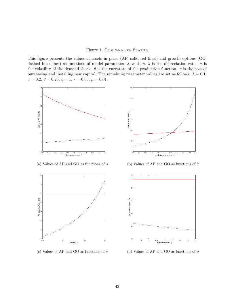
Figure 1: Comparative Statics

This figure presents the values of assets in place (AP, solid red lines) and growth options (GO,dashed blue lines) as functions of model parameters λ, σ, θ, η. λ is the depreciation rate. σ isthe volatility of the demand shock. θ is the curvature of the production function. η is the cost ofpurchasing and installing new capital. The remaining parameter values are set as follows: λ = 0.1,σ = 0.2, θ = 0.25, η = 1, r = 0.05, µ = 0.01.

(a) Values of AP and GO as functions of λ (b) Values of AP and GO as functions of θ

(c) Values of AP and GO as functions of σ (d) Values of AP and GO as functions of η

43

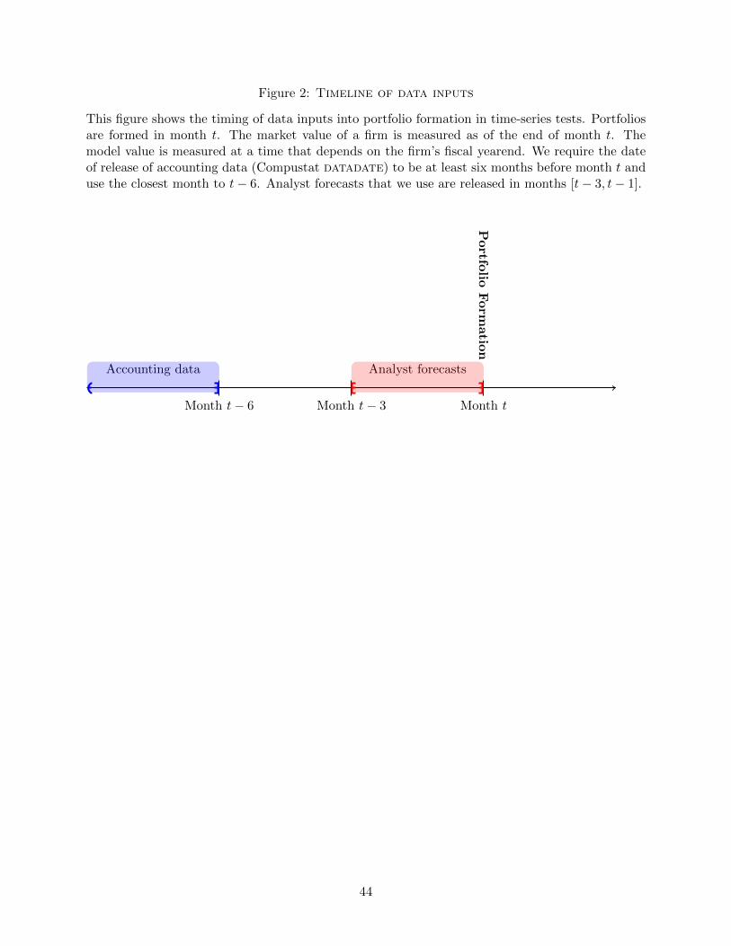
Figure 2: Timeline of data inputs

This figure shows the timing of data inputs into portfolio formation in time-series tests. Portfoliosare formed in month t. The market value of a firm is measured as of the end of month t. Themodel value is measured at a time that depends on the firm’s fiscal yearend. We require the dateof release of accounting data (Compustat datadate) to be at least six months before month t anduse the closest month to t− 6. Analyst forecasts that we use are released in months [t− 3, t− 1].

Month t− 6 Month t− 3 Month t

Analyst forecastsAccounting data

Portfo

lioForm

atio

n

44

Tab

le1:Desc

riptivestatisticsofvariablesuse

din

misvaluationest

imation

Th

ista

ble

pro

vid

essu

mm

ary

stat

isti

csfo

rth

em

ain

vari

ab

les

use

din

esti

mati

on

.T

he

sam

ple

isb

ase

don

2014

Ind

ust

rial

Com

pu

stat

An

nu

al

an

dQ

uar

terl

yF

un

dam

enta

lF

iles

,C

ente

rfo

rR

esea

rch

inS

ecu

rity

Pri

ces

(CR

SP

),an

dIn

stit

uti

on

al

Bro

kers

Est

imate

Syst

em(I

BE

S).

Th

esa

mp

leco

vers

the

per

iod

from

Jan

uar

y19

80to

Dec

emb

er20

14.

Vari

ab

les

are

eith

erat

the

month

lyor

an

nu

al

freq

uen

cy.

Th

ela

stco

lum

nin

the

tab

lein

dic

ate

sth

efr

equ

ency

wit

hw

hic

ha

give

nva

riab

leis

obse

rved

.M

ark

etva

lue

of

equ

ity,

cap

ital,

reve

nu

e,C

OG

S,

SG

&A

,E

BIT

DA

,lo

ng-t

erm

an

dsh

ort

-ter

md

ebt

are

inm

illi

ons

ofd

olla

rs.

Var

iab

les

are

defi

ned

inT

ab

leA

1.

Mea

nS

t.D

ev.

10%

25%

50%

75%

90%

#O

bs.

Fre

qu

ency

Fir

mC

har

acte

rist

ics

Mar

ket

valu

eof

equ

ity

1,8

90.8

811,2

72.7

58.4

927.1

3127.0

4649.8

22,6

50.4

51,5

06,7

19

Month

lyC

apit

al1,0

02.2

66,5

33.9

83.9

913.5

261.6

7323.1

41,4

66.5

1129,8

76

An

nu

al

Rev

enue

1,6

02.5

98,6

10.1

615.2

545.4

1169.0

1706.3

42,6

20.3

5129,8

76

An

nu

al

Cos

tof

good

sso

ld1,0

79.7

36,3

88.6

97.6

525.0

9100.8

9444.0

01,7

27.4

8129,8

76

An

nu

al

SG

&A

280.7

91,4

57.4

72.9

68.5

631.1

5127.0

3463.0

1129,8

76

An

nu

al

EB

ITD

A242.0

71,4

09.6

21.2

24.3

218.6

991.1

0360.8

7129,8

76

An

nu

al

Lon

g-te

rmd

ebt

386.1

03,3

86.8

40.0

00.9

613.6

2121.1

0596.4

5129,6

45

An

nu

al

Sh

ort-

term

deb

t127.9

72,3

15.1

30.0

00.2

02.2

313.0

469.6

0129,7

42

An

nu

al

Equ

ity

bet

a1.1

30.7

50.2

50.6

61.0

81.5

62.1

11,3

23,7

80

Month

ly

Ind

ust

ryC

har

acte

rist

ics

Dem

and

grow

thra

te0.0

30.0

10.0

20.0

30.0

30.0

40.0

425,2

60

Month

lyD

eman

dvol

atil

ity

0.1

90.2

70.0

80.1

10.1

50.2

00.2

827,4

47

Month

lyC

apit

ald

epre

ciat

ion

rate

0.0

90.0

40.0

50.0

70.0

80.1

10.1

427,6

50

Month

ly

45

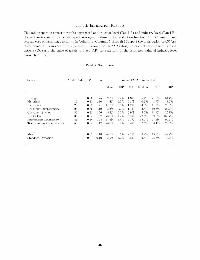
Table 2: Estimation Results

This table reports estimation results aggregated at the sector level (Panel A) and industry level (Panel B).

For each sector and industry, we report average curvature of the production function, θ, in Column 3, and

average cost of installing capital, η, in Column 4. Columns 5 through 10 report the distribution of GO/AP

ratios across firms in each industry/sector. To compute GO/AP ratios, we calculate the value of growth

options (GO) and the value of assets in place (AP) for each firm at the estimated value of industry-level

parameters (θ, η).

Panel A: Sector Level

Sector GICS Code θ η Value of GO / Value of AP

Mean 10P 25P Median 75P 90P

Energy 10 0.30 1.25 32.2% 0.2% 1.3% 5.4% 21.0% 54.7%Materials 15 0.33 1.30 3.4% 0.0% 0.1% 0.7% 2.7% 7.5%Industrials 20 0.32 1.21 11.7% 0.3% 1.2% 4.0% 11.9% 28.8%Consumer Discretionary 25 0.30 1.19 8.3% 0.2% 1.1% 3.8% 10.3% 20.2%Consumer Staples 30 0.31 1.26 9.3% 0.2% 0.9% 3.6% 11.1% 25.1%Health Care 35 0.34 1.07 73.1% 1.7% 6.7% 22.5% 59.8% 153.7%Information Technology 45 0.36 1.04 53.6% 1.4% 4.1% 12.2% 35.6% 92.3%Telecommunication Services 50 0.34 1.17 26.1% 0.1% 0.4% 2.5% 8.4% 29.8%

Mean 0.32 1.18 24.5% 0.6% 2.1% 6.9% 19.8% 49.2%Standard Deviation 0.04 0.10 35.9% 1.2% 3.5% 9.8% 25.3% 73.2%

46

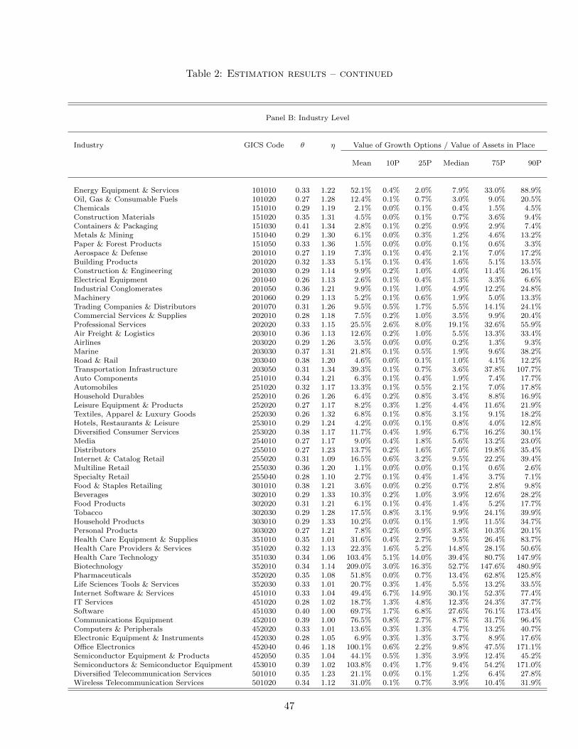
Table 2: Estimation results – continued

Panel B: Industry Level

Industry GICS Code θ η Value of Growth Options / Value of Assets in Place

Mean 10P 25P Median 75P 90P

Energy Equipment & Services 101010 0.33 1.22 52.1% 0.4% 2.0% 7.9% 33.0% 88.9%Oil, Gas & Consumable Fuels 101020 0.27 1.28 12.4% 0.1% 0.7% 3.0% 9.0% 20.5%Chemicals 151010 0.29 1.19 2.1% 0.0% 0.1% 0.4% 1.5% 4.5%Construction Materials 151020 0.35 1.31 4.5% 0.0% 0.1% 0.7% 3.6% 9.4%Containers & Packaging 151030 0.41 1.34 2.8% 0.1% 0.2% 0.9% 2.9% 7.4%Metals & Mining 151040 0.29 1.30 6.1% 0.0% 0.3% 1.2% 4.6% 13.2%Paper & Forest Products 151050 0.33 1.36 1.5% 0.0% 0.0% 0.1% 0.6% 3.3%Aerospace & Defense 201010 0.27 1.19 7.3% 0.1% 0.4% 2.1% 7.0% 17.2%Building Products 201020 0.32 1.33 5.1% 0.1% 0.4% 1.6% 5.1% 13.5%Construction & Engineering 201030 0.29 1.14 9.9% 0.2% 1.0% 4.0% 11.4% 26.1%Electrical Equipment 201040 0.26 1.13 2.6% 0.1% 0.4% 1.3% 3.3% 6.6%Industrial Conglomerates 201050 0.36 1.21 9.9% 0.1% 1.0% 4.9% 12.2% 24.8%Machinery 201060 0.29 1.13 5.2% 0.1% 0.6% 1.9% 5.0% 13.3%Trading Companies & Distributors 201070 0.31 1.26 9.5% 0.5% 1.7% 5.5% 14.1% 24.1%Commercial Services & Supplies 202010 0.28 1.18 7.5% 0.2% 1.0% 3.5% 9.9% 20.4%Professional Services 202020 0.33 1.15 25.5% 2.6% 8.0% 19.1% 32.6% 55.9%Air Freight & Logistics 203010 0.36 1.13 12.6% 0.2% 1.0% 5.5% 13.3% 33.4%Airlines 203020 0.29 1.26 3.5% 0.0% 0.0% 0.2% 1.3% 9.3%Marine 203030 0.37 1.31 21.8% 0.1% 0.5% 1.9% 9.6% 38.2%Road & Rail 203040 0.38 1.20 4.6% 0.0% 0.1% 1.0% 4.1% 12.2%Transportation Infrastructure 203050 0.31 1.34 39.3% 0.1% 0.7% 3.6% 37.8% 107.7%Auto Components 251010 0.34 1.21 6.3% 0.1% 0.4% 1.9% 7.4% 17.7%Automobiles 251020 0.32 1.17 13.3% 0.1% 0.5% 2.1% 7.0% 17.8%Household Durables 252010 0.26 1.26 6.4% 0.2% 0.8% 3.4% 8.8% 16.9%Leisure Equipment & Products 252020 0.27 1.17 8.2% 0.3% 1.2% 4.4% 11.6% 21.9%Textiles, Apparel & Luxury Goods 252030 0.26 1.32 6.8% 0.1% 0.8% 3.1% 9.1% 18.2%Hotels, Restaurants & Leisure 253010 0.29 1.24 4.2% 0.0% 0.1% 0.8% 4.0% 12.8%Diversified Consumer Services 253020 0.38 1.17 11.7% 0.4% 1.9% 6.7% 16.2% 30.1%Media 254010 0.27 1.17 9.0% 0.4% 1.8% 5.6% 13.2% 23.0%Distributors 255010 0.27 1.23 13.7% 0.2% 1.6% 7.0% 19.8% 35.4%Internet & Catalog Retail 255020 0.31 1.09 16.5% 0.6% 3.2% 9.5% 22.2% 39.4%Multiline Retail 255030 0.36 1.20 1.1% 0.0% 0.0% 0.1% 0.6% 2.6%Specialty Retail 255040 0.28 1.10 2.7% 0.1% 0.4% 1.4% 3.7% 7.1%Food & Staples Retailing 301010 0.38 1.21 3.6% 0.0% 0.2% 0.7% 2.8% 9.8%Beverages 302010 0.29 1.33 10.3% 0.2% 1.0% 3.9% 12.6% 28.2%Food Products 302020 0.31 1.21 6.1% 0.1% 0.4% 1.4% 5.2% 17.7%Tobacco 302030 0.29 1.28 17.5% 0.8% 3.1% 9.9% 24.1% 39.9%Household Products 303010 0.29 1.33 10.2% 0.0% 0.1% 1.9% 11.5% 34.7%Personal Products 303020 0.27 1.21 7.8% 0.2% 0.9% 3.8% 10.3% 20.1%Health Care Equipment & Supplies 351010 0.35 1.01 31.6% 0.4% 2.7% 9.5% 26.4% 83.7%Health Care Providers & Services 351020 0.32 1.13 22.3% 1.6% 5.2% 14.8% 28.1% 50.6%Health Care Technology 351030 0.34 1.06 103.4% 5.1% 14.0% 39.4% 80.7% 147.9%Biotechnology 352010 0.34 1.14 209.0% 3.0% 16.3% 52.7% 147.6% 480.9%Pharmaceuticals 352020 0.35 1.08 51.8% 0.0% 0.7% 13.4% 62.8% 125.8%Life Sciences Tools & Services 352030 0.33 1.01 20.7% 0.3% 1.4% 5.5% 13.2% 33.5%Internet Software & Services 451010 0.33 1.04 49.4% 6.7% 14.9% 30.1% 52.3% 77.4%IT Services 451020 0.28 1.02 18.7% 1.3% 4.8% 12.3% 24.3% 37.7%Software 451030 0.40 1.00 69.7% 1.7% 6.8% 27.6% 76.1% 173.4%Communications Equipment 452010 0.39 1.00 76.5% 0.8% 2.7% 8.7% 31.7% 96.4%Computers & Peripherals 452020 0.33 1.01 13.6% 0.3% 1.3% 4.7% 13.2% 40.7%Electronic Equipment & Instruments 452030 0.28 1.05 6.9% 0.3% 1.3% 3.7% 8.9% 17.6%Office Electronics 452040 0.46 1.18 100.1% 0.6% 2.2% 9.8% 47.5% 171.1%Semiconductor Equipment & Products 452050 0.35 1.04 44.1% 0.5% 1.3% 3.9% 12.4% 45.2%Semiconductors & Semiconductor Equipment 453010 0.39 1.02 103.8% 0.4% 1.7% 9.4% 54.2% 171.0%Diversified Telecommunication Services 501010 0.35 1.23 21.1% 0.0% 0.1% 1.2% 6.4% 27.8%Wireless Telecommunication Services 501020 0.34 1.12 31.0% 0.1% 0.7% 3.9% 10.4% 31.9%

47

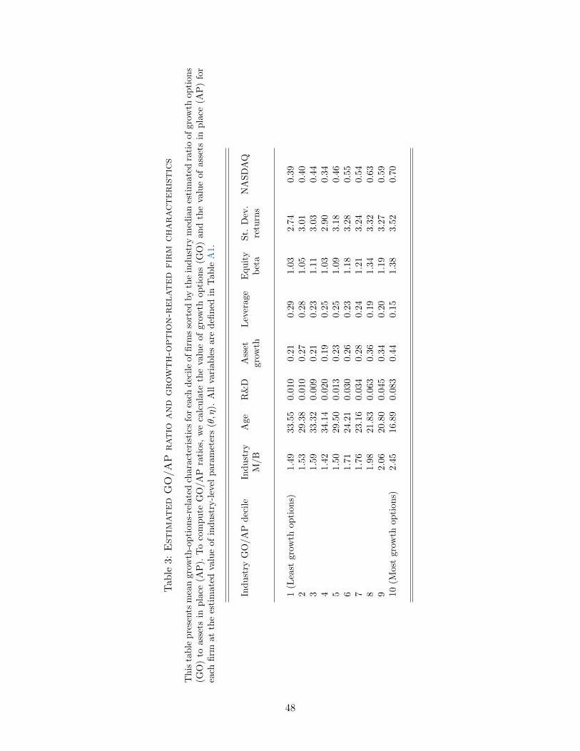
Tab

le3:

Est

imated

GO/AP

ratio

and

growth-o

ption-related

firm

characteristics

Th

ista

ble

pre

sents

mea

ngr

owth

-op

tion

s-re

late

dch

ara

cter

isti

csfo

rea

chdec

ile

of

firm

sso

rted

by

the

ind

ust

rym

edia

nes

tim

ate

dra

tio

of

gro

wth

op

tion

s(G

O)

toas

sets

inp

lace

(AP

).T

oco

mp

ute

GO

/A

Pra

tios,

we

calc

ula

teth

eva

lue

of

gro

wth

op

tion

s(G

O)

an

dth

eva

lue

of

ass

ets

inp

lace

(AP

)fo

rea

chfi

rmat

the

esti

mat

edva

lue

ofin

du

stry

-lev

elpara

met

ers

(θ,η

).A

llva

riab

les

are

defi

ned

inT

ab

leA

1.

Ind

ust

ryG

O/A

Pd

ecil

eIn

du

stry

Age

R&

DA

sset

Lev

erage

Equ

ity

St.

Dev

.N

AS

DA

QM

/B

gro

wth

bet

are

turn

s

1(L

east

grow

thop

tion

s)1.4

933.5

50.0

10

0.2

10.2

91.0

32.7

40.3

92

1.5

329.3

80.0

10

0.2

70.2

81.0

53.0

10.4

03

1.5

933.3

20.0

09

0.2

10.2

31.1

13.0

30.4

44

1.4

234.1

40.0

20

0.1

90.2

51.0

32.9

00.3

45

1.5

029.5

00.0

13

0.2

30.2

51.0

93.1

80.4

66

1.7

124.2

10.0

30

0.2

60.2

31.1

83.2

80.5

57

1.7

623.1

60.0

34

0.2

80.2

41.2

13.2

40.5

48

1.9

821.8

30.0

63

0.3

60.1

91.3

43.3

20.6

39

2.0

620.8

00.0

45

0.3

40.2

01.1

93.2

70.5

910

(Mos

tgr

owth

opti

ons)

2.4

516.8

90.0

83

0.4

40.1

51.3

83.5

20.7

0

48

Tab

le4:

Misvaluationand

firm

characteristics

Th

ista

ble

pre

sents

mea

nch

ara

cter

isti

csof

firm

sin

each

mis

valu

ati

on

dec

ile.

Valu

ati

on

dec

ile

“U

”d

enote

sth

em

ost

un

der

valu

edd

ecile.

Dec

ile

“O

”d

enote

sth

em

ost

over

valu

ed.

Mis

valu

ati

on

isco

mp

ute

dacc

ord

ing

to(7

).A

llvari

ab

les

are

defi

ned

inT

ab

leA

1.

Mis

valu

ati

on

Ass

ets

MV

Age

Ind

ust

ryR

&D

Ass

etIn

ves

t-P

rofi

t-N

et6-m

onth

St.

Dev

.A

mih

ud

Inst

itu

tion

al

Nu

mb

erof

Fore

cast

dec

ile

equ

ity

M/B

gro

wth

men

tab

ilit

yis

suan

cere

turn

of

retu

rns

mea

sure

ow

ner

ship

an

aly

sts

dis

per

sion

U1,9

01

1,8

53

20.0

91.8

30.0

39

0.2

96

0.0

55

0.1

22

0.0

27

-5.5

13.5

60.4

90.4

43.9

00.1

22

22,4

27

2,2

41

26.7

01.7

00.0

26

0.2

06

0.0

53

0.1

04

0.0

16

-1.3

23.1

80.4

00.5

14.1

70.0

84

32,4

20

2,2

42

29.4

51.6

70.0

23

0.1

90

0.0

53

0.0

99

0.0

16

2.0

42.9

60.3

20.5

34.4

40.0

75

42,4

08

2,3

76

31.7

21.6

60.0

23

0.1

97

0.0

54

0.0

98

0.0

15

4.5

82.8

40.2

80.5

64.4

70.0

63

52,3

95

2,3

82

32.4

61.6

60.0

24

0.2

06

0.0

57

0.0

98

0.0

17

6.9

62.8

10.2

60.5

74.6

70.0

67

62,3

07

2,3

90

32.5

71.6

80.0

25

0.2

25

0.0

63

0.0

98

0.0

20

8.9

72.8

10.2

40.5

84.7

60.0

64

72,2

97

2,5

13

30.6

31.7

00.0

27

0.2

61

0.0

75

0.0

96

0.0

28

10.8

72.8

90.2

50.5

74.7

90.0

55

82,1

65

2,4

73

26.9

51.7

40.0

30

0.3

14

0.0

89

0.0

91

0.0

37

13.4

73.0

50.2

60.5

74.7

50.0

54

91,6

10

2,0

72

21.5

91.8

00.0

39

0.3

88

0.1

04

0.0

75

0.0

52

16.2

83.3

80.3

10.5

44.6

90.0

56

O651

1,1

14

15.2

51.8

90.0

52

0.4

74

0.1

14

0.0

18

0.0

74

17.2

73.9

30.4

40.4

73.9

10.0

99

49

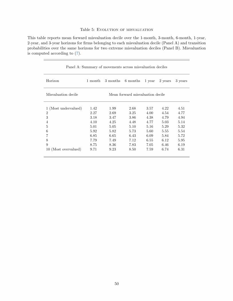
Table 5: Evolution of misvaluation

This table reports mean forward misvaluation decile over the 1-month, 3-month, 6-month, 1-year,2-year, and 3-year horizons for firms belonging to each misvaluation decile (Panel A) and transitionprobabilities over the same horizons for two extreme misvaluation deciles (Panel B). Misvaluationis computed according to (7).

Panel A: Summary of movements across misvaluation deciles

Horizon 1 month 3 months 6 months 1 year 2 years 3 years

Misvaluation decile Mean forward misvaluation decile

1 (Most undervalued) 1.42 1.99 2.68 3.57 4.22 4.512 2.27 2.69 3.25 4.00 4.54 4.773 3.18 3.47 3.86 4.38 4.79 4.944 4.10 4.25 4.48 4.77 5.03 5.145 5.01 5.05 5.10 5.16 5.29 5.326 5.92 5.82 5.73 5.60 5.55 5.547 6.85 6.65 6.43 6.09 5.84 5.728 7.79 7.49 7.12 6.55 6.12 5.959 8.75 8.36 7.83 7.05 6.46 6.1910 (Most overvalued) 9.71 9.23 8.50 7.59 6.74 6.31

50

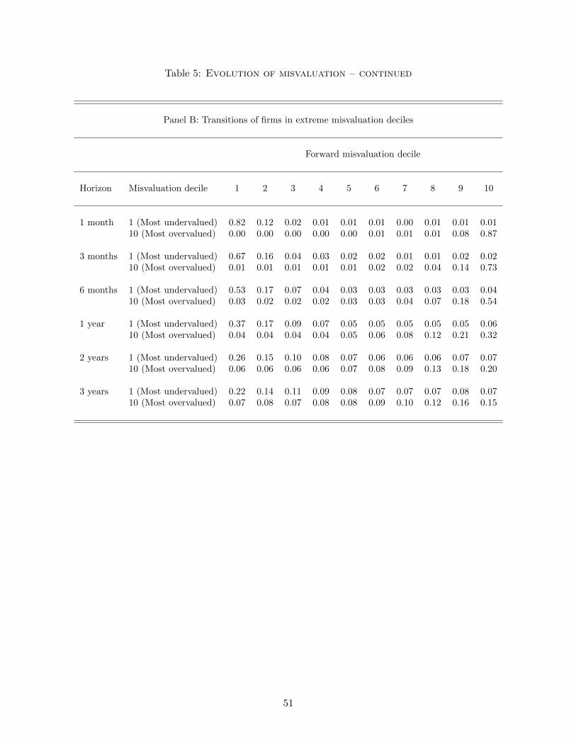
Table 5: Evolution of misvaluation – continued

Panel B: Transitions of firms in extreme misvaluation deciles

Forward misvaluation decile

Horizon Misvaluation decile 1 2 3 4 5 6 7 8 9 10

1 month 1 (Most undervalued) 0.82 0.12 0.02 0.01 0.01 0.01 0.00 0.01 0.01 0.0110 (Most overvalued) 0.00 0.00 0.00 0.00 0.00 0.01 0.01 0.01 0.08 0.87

3 months 1 (Most undervalued) 0.67 0.16 0.04 0.03 0.02 0.02 0.01 0.01 0.02 0.0210 (Most overvalued) 0.01 0.01 0.01 0.01 0.01 0.02 0.02 0.04 0.14 0.73

6 months 1 (Most undervalued) 0.53 0.17 0.07 0.04 0.03 0.03 0.03 0.03 0.03 0.0410 (Most overvalued) 0.03 0.02 0.02 0.02 0.03 0.03 0.04 0.07 0.18 0.54

1 year 1 (Most undervalued) 0.37 0.17 0.09 0.07 0.05 0.05 0.05 0.05 0.05 0.0610 (Most overvalued) 0.04 0.04 0.04 0.04 0.05 0.06 0.08 0.12 0.21 0.32

2 years 1 (Most undervalued) 0.26 0.15 0.10 0.08 0.07 0.06 0.06 0.06 0.07 0.0710 (Most overvalued) 0.06 0.06 0.06 0.06 0.07 0.08 0.09 0.13 0.18 0.20

3 years 1 (Most undervalued) 0.22 0.14 0.11 0.09 0.08 0.07 0.07 0.07 0.08 0.0710 (Most overvalued) 0.07 0.08 0.07 0.08 0.08 0.09 0.10 0.12 0.16 0.15

51

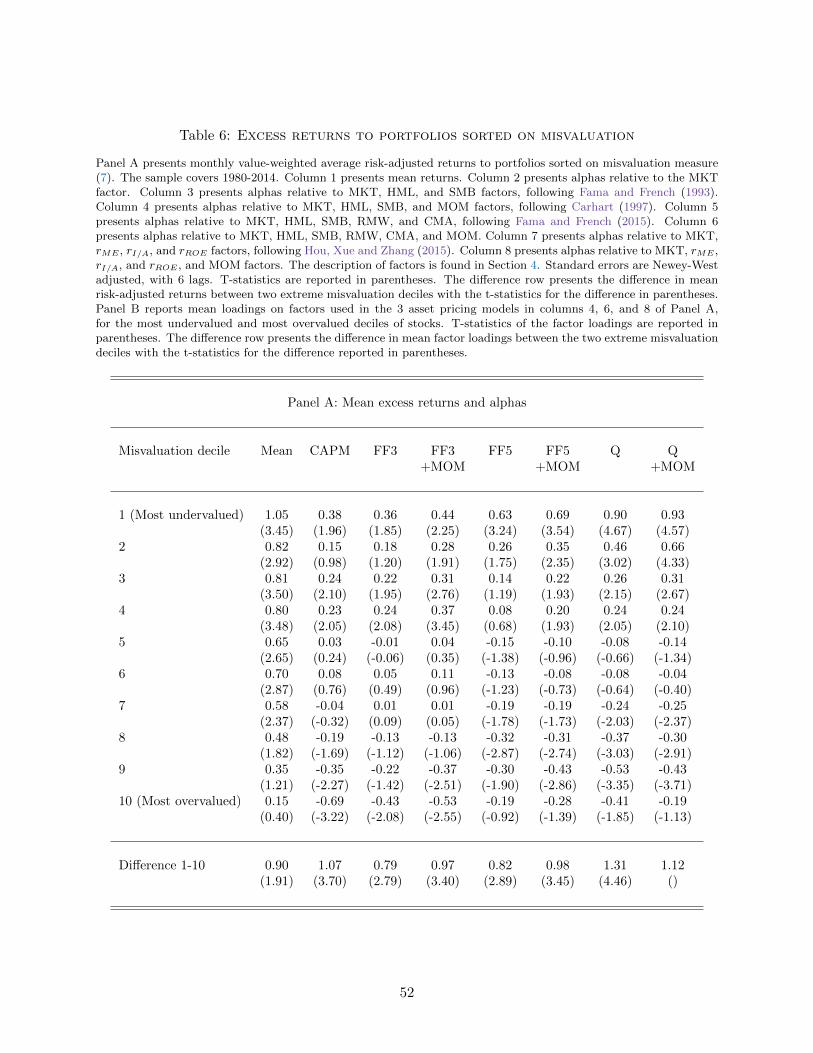
Table 6: Excess returns to portfolios sorted on misvaluation

Panel A presents monthly value-weighted average risk-adjusted returns to portfolios sorted on misvaluation measure(7). The sample covers 1980-2014. Column 1 presents mean returns. Column 2 presents alphas relative to the MKTfactor. Column 3 presents alphas relative to MKT, HML, and SMB factors, following Fama and French (1993).Column 4 presents alphas relative to MKT, HML, SMB, and MOM factors, following Carhart (1997). Column 5presents alphas relative to MKT, HML, SMB, RMW, and CMA, following Fama and French (2015). Column 6presents alphas relative to MKT, HML, SMB, RMW, CMA, and MOM. Column 7 presents alphas relative to MKT,rME , rI/A, and rROE factors, following Hou, Xue and Zhang (2015). Column 8 presents alphas relative to MKT, rME ,rI/A, and rROE , and MOM factors. The description of factors is found in Section 4. Standard errors are Newey-Westadjusted, with 6 lags. T-statistics are reported in parentheses. The difference row presents the difference in meanrisk-adjusted returns between two extreme misvaluation deciles with the t-statistics for the difference in parentheses.Panel B reports mean loadings on factors used in the 3 asset pricing models in columns 4, 6, and 8 of Panel A,for the most undervalued and most overvalued deciles of stocks. T-statistics of the factor loadings are reported inparentheses. The difference row presents the difference in mean factor loadings between the two extreme misvaluationdeciles with the t-statistics for the difference reported in parentheses.

Panel A: Mean excess returns and alphas

Misvaluation decile Mean CAPM FF3 FF3 FF5 FF5 Q Q+MOM +MOM +MOM

1 (Most undervalued) 1.05 0.38 0.36 0.44 0.63 0.69 0.90 0.93(3.45) (1.96) (1.85) (2.25) (3.24) (3.54) (4.67) (4.57)

2 0.82 0.15 0.18 0.28 0.26 0.35 0.46 0.66(2.92) (0.98) (1.20) (1.91) (1.75) (2.35) (3.02) (4.33)

3 0.81 0.24 0.22 0.31 0.14 0.22 0.26 0.31(3.50) (2.10) (1.95) (2.76) (1.19) (1.93) (2.15) (2.67)

4 0.80 0.23 0.24 0.37 0.08 0.20 0.24 0.24(3.48) (2.05) (2.08) (3.45) (0.68) (1.93) (2.05) (2.10)

5 0.65 0.03 -0.01 0.04 -0.15 -0.10 -0.08 -0.14(2.65) (0.24) (-0.06) (0.35) (-1.38) (-0.96) (-0.66) (-1.34)

6 0.70 0.08 0.05 0.11 -0.13 -0.08 -0.08 -0.04(2.87) (0.76) (0.49) (0.96) (-1.23) (-0.73) (-0.64) (-0.40)

7 0.58 -0.04 0.01 0.01 -0.19 -0.19 -0.24 -0.25(2.37) (-0.32) (0.09) (0.05) (-1.78) (-1.73) (-2.03) (-2.37)

8 0.48 -0.19 -0.13 -0.13 -0.32 -0.31 -0.37 -0.30(1.82) (-1.69) (-1.12) (-1.06) (-2.87) (-2.74) (-3.03) (-2.91)

9 0.35 -0.35 -0.22 -0.37 -0.30 -0.43 -0.53 -0.43(1.21) (-2.27) (-1.42) (-2.51) (-1.90) (-2.86) (-3.35) (-3.71)

10 (Most overvalued) 0.15 -0.69 -0.43 -0.53 -0.19 -0.28 -0.41 -0.19(0.40) (-3.22) (-2.08) (-2.55) (-0.92) (-1.39) (-1.85) (-1.13)

Difference 1-10 0.90 1.07 0.79 0.97 0.82 0.98 1.31 1.12(1.91) (3.70) (2.79) (3.40) (2.89) (3.45) (4.46) ()

52

Tab

le6:Excess

returnsto

portfoliosso

rted

onmisvaluation–Continued

Pan

elB

:F

act

or

Load

ings

Mod

elM

isva

luat

ion

Dec

ile

MK

TS

MB

HM

LR

MW

CM

Ar M

Er I

/A

r ROE

MO

M

FF

3+M

OM

Mos

tu

nd

erva

lued

1.0

7-0

.11

-0.0

2-0

.11

(23.8

5)

(-1.6

8)

(-0.2

7)

(-2.6

4)

Mos

tov

erva

lued

1.2

40.2

2-0

.39

0.1

3(2

6.3

7)

(3.1

4)

(-5.3

5)

(3.0

3)

Diff

eren

ce-0

.17

-0.3

30.3

7-0

.25

(-2.6

0)

(-3.4

3)

(3.6

8)

(-4.0

1)

FF

5+M

OM

Mos

tu

nd

erva

lued

0.9

7-0

.10

0.1

7-0

.35

-0.4

6-0

.10

(20.7

8)

(-1.5

8)

(1.9

6)

(-4.2

2)

(-3.5

8)

(-2.3

4)

Mos

tov

erva

lued

1.1

60.1

8-0

.33

-0.4

7-0

.16

0.1

5(2

3.5

8)

(2.6

7)

(-3.6

5)

(-5.4

0)

(-1.1

7)

(3.4

2)

Diff

eren

ce-0

.18

-0.2

90.5

10.1

2-0

.30

-0.2

4(-

2.6

9)

(-3.0

2)

(3.9

9)

(0.9

9)

(-1.6

3)

(-4.0

9)

Q+

MO

MM

ost

un

der

valu

ed0.9

20.1

0-0

.50

-0.4

20.0

0(2

0.9

5)

(1.5

0)

(-4.9

5)

(-4.9

3)

(0.0

3)

Mos

tov

erva

lued

1.2

10.1

8-0

.50

-0.2

50.1

9(2

4.4

0)

(2.4

5)

(-4.3

9)

(-2.6

2)

(3.5

6)

Diff

eren

ce-0

.29

-0.0

80.0

0-0

.17

-0.1

9(-

4.4

4)

(-0.8

5)

(0.0

2)

(-1.2

9)

(-2.6

5)

53

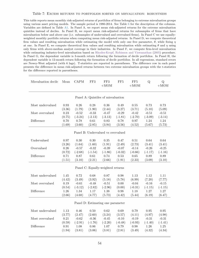
Table 7: Excess returns to portfolios sorted on misvaluation: robustness

This table reports mean monthly risk-adjusted returns of portfolios of firms belonging to extreme misvaluation groupsusing various asset pricing models. The sample period is 1980-2014. See Table 6 for the description of the columns.Variables are defined in Table A1. In Panel A, we report mean risk-adjusted returns for the extreme misvaluationquintiles instead of deciles. In Panel B, we report mean risk-adjusted returns for subsamples of firms that havemisvaluation below and above one (i.e. subsamples of undervalued and overvalued firms). In Panel C we use equally-weighted monthly portfolio returns when computing mean risk-adjusted returns. In Panel D, we compute theoreticalfirm values and resulting misvaluation while estimating the model with only one free parameter, θ, while fixing ηat one. In Panel E, we compute theoretical firm values and resulting misvaluation while estimating θ and η usingonly firms with above-median analyst coverage in their industries. In Panel F, we compute firm-level misvaluationwhile estimating industry-level misvaluation based on Rhodes-Kropf, Robinson and Viswanathan (2005) procedure.In Panel G, the dependent variable is 3-month return following the formation of decile portfolios. In Panel H, thedependent variable is 12-month return following the formation of decile portfolios. In all regressions, standard errorsare Newey-West adjusted (with 6 lags). T-statistics are reported in parentheses. The difference row in each panelpresents the difference in mean risk-adjusted returns between two extreme misvaluation groups with the t-statisticsfor the difference reported in parentheses.

Misvaluation decile Mean CAPM FF3 FF3 FF5 FF5 Q Q+MOM +MOM +MOM

Panel A: Quintiles of misvaluation

Most undervalued 0.93 0.26 0.28 0.36 0.49 0.55 0.73 0.73(3.36) (1.79) (1.90) (2.44) (3.27) (3.71) (5.10) (5.09)

Most overvalued 0.23 -0.52 -0.33 -0.47 -0.29 -0.42 -0.51 -0.51(0.75) (-3.24) (-2.13) (-3.13) (-1.81) (-2.70) (-3.09) (-3.14)

Difference 0.70 0.78 0.61 0.83 0.78 0.97 1.24 1.24(1.69) (3.60) (2.85) (3.94) (3.56) (4.52) (5.67) (5.73)

Panel B: Undervalued vs overvalued

Undervalued 0.97 0.30 0.30 0.35 0.47 0.51 0.64 0.64(3.26) (1.64) (1.60) (1.91) (2.49) (2.73) (3.41) (3.41)

Overvalued 0.26 -0.57 -0.32 -0.39 -0.07 -0.14 -0.26 -0.25(0.72) (-2.68) (-1.54) (-1.86) (-0.32) (-0.66) (-1.17) (-1.16)

Difference 0.71 0.87 0.61 0.74 0.53 0.65 0.89 0.89(1.51) (3.10) (2.21) (2.66) (1.91) (2.33) (3.09) (3.10)

Panel C: Equally-weighted returns

Most undervalued 1.45 0.72 0.68 0.87 0.98 1.13 1.12 1.11(4.42) (3.49) (3.92) (5.18) (5.78) (6.99) (7.20) (7.77)

Most overvalued 0.19 -0.61 -0.48 -0.51 0.00 -0.04 -0.16 -0.15(0.54) (-3.12) (-2.82) (-2.96) (0.00) (-0.31) (-1.15) (-1.15)

Difference 1.26 1.34 1.17 1.38 0.98 1.18 1.27 1.27(2.66) (4.68) (4.77) (5.73) (4.42) (5.44) (6.19) (6.47)

Panel D: Estimating one parameter

Most undervalued 1.13 0.46 0.50 0.62 0.69 0.79 0.95 0.95(3.77) (2.47) (2.60) (3.24) (3.57) (4.11) (4.97) (4.98)

Most overvalued 0.21 -0.62 -0.36 -0.45 -0.10 -0.19 -0.31 -0.31(0.59) (-2.91) (-1.76) (-2.20) (-0.48) (-0.93) (-1.40) (-1.41)

Difference 0.91 1.08 0.86 1.07 0.79 0.98 1.26 1.25(1.94) (3.81) (3.06) (3.81) (2.81) (3.49) (4.32) (4.34)

54

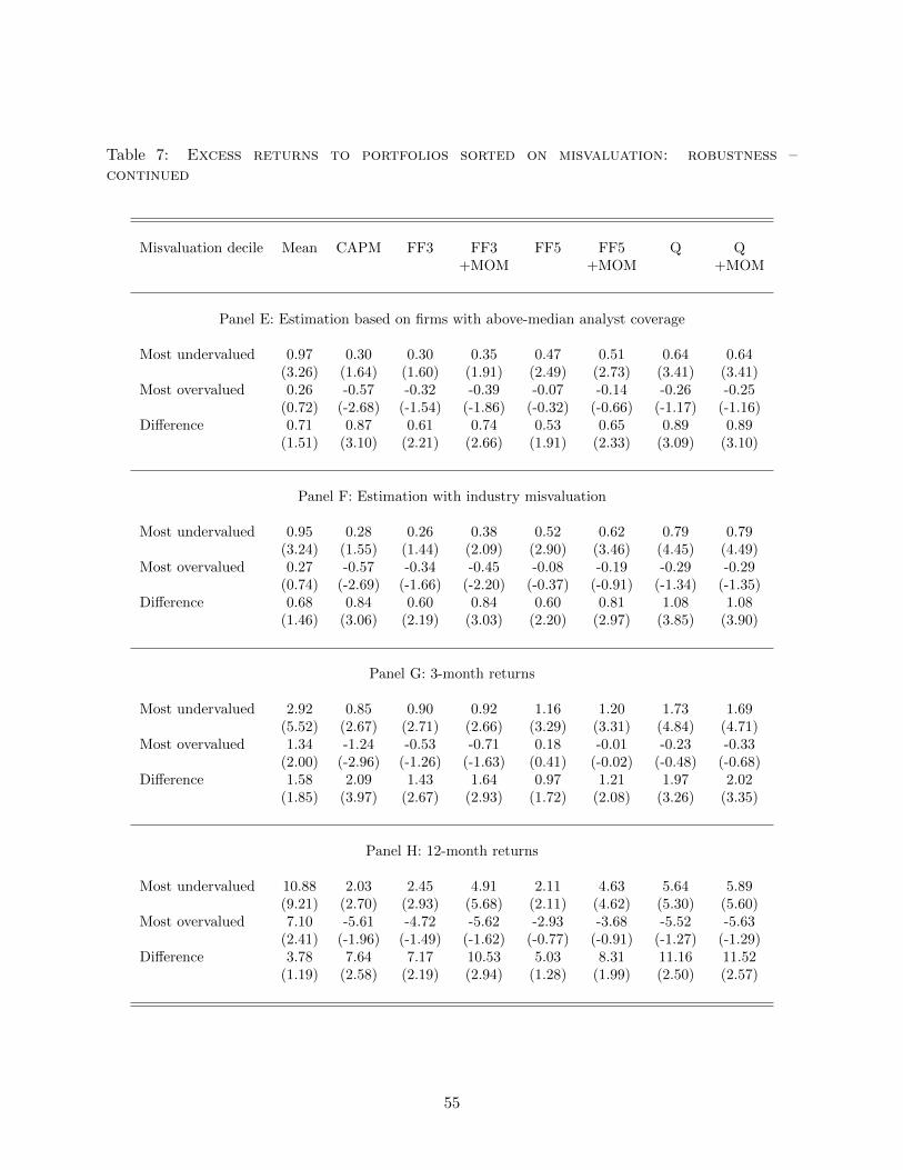
Table 7: Excess returns to portfolios sorted on misvaluation: robustness –continued

Misvaluation decile Mean CAPM FF3 FF3 FF5 FF5 Q Q+MOM +MOM +MOM

Panel E: Estimation based on firms with above-median analyst coverage

Most undervalued 0.97 0.30 0.30 0.35 0.47 0.51 0.64 0.64(3.26) (1.64) (1.60) (1.91) (2.49) (2.73) (3.41) (3.41)

Most overvalued 0.26 -0.57 -0.32 -0.39 -0.07 -0.14 -0.26 -0.25(0.72) (-2.68) (-1.54) (-1.86) (-0.32) (-0.66) (-1.17) (-1.16)

Difference 0.71 0.87 0.61 0.74 0.53 0.65 0.89 0.89(1.51) (3.10) (2.21) (2.66) (1.91) (2.33) (3.09) (3.10)

Panel F: Estimation with industry misvaluation

Most undervalued 0.95 0.28 0.26 0.38 0.52 0.62 0.79 0.79(3.24) (1.55) (1.44) (2.09) (2.90) (3.46) (4.45) (4.49)

Most overvalued 0.27 -0.57 -0.34 -0.45 -0.08 -0.19 -0.29 -0.29(0.74) (-2.69) (-1.66) (-2.20) (-0.37) (-0.91) (-1.34) (-1.35)

Difference 0.68 0.84 0.60 0.84 0.60 0.81 1.08 1.08(1.46) (3.06) (2.19) (3.03) (2.20) (2.97) (3.85) (3.90)

Panel G: 3-month returns

Most undervalued 2.92 0.85 0.90 0.92 1.16 1.20 1.73 1.69(5.52) (2.67) (2.71) (2.66) (3.29) (3.31) (4.84) (4.71)

Most overvalued 1.34 -1.24 -0.53 -0.71 0.18 -0.01 -0.23 -0.33(2.00) (-2.96) (-1.26) (-1.63) (0.41) (-0.02) (-0.48) (-0.68)

Difference 1.58 2.09 1.43 1.64 0.97 1.21 1.97 2.02(1.85) (3.97) (2.67) (2.93) (1.72) (2.08) (3.26) (3.35)

Panel H: 12-month returns

Most undervalued 10.88 2.03 2.45 4.91 2.11 4.63 5.64 5.89(9.21) (2.70) (2.93) (5.68) (2.11) (4.62) (5.30) (5.60)

Most overvalued 7.10 -5.61 -4.72 -5.62 -2.93 -3.68 -5.52 -5.63(2.41) (-1.96) (-1.49) (-1.62) (-0.77) (-0.91) (-1.27) (-1.29)

Difference 3.78 7.64 7.17 10.53 5.03 8.31 11.16 11.52(1.19) (2.58) (2.19) (2.94) (1.28) (1.99) (2.50) (2.57)

55

Table 8: Fama-MacBeth regressions of returns on misvaluation measure

This table presents results of estimating cross-sectional regressions of returns on the natural logarithm ofmisvaluation measure and the following characteristics: the natural logarithm of equity book to market ratio,the natural logarithm of market value, investment-to-assets ratio, gross profitability-to-assets ratio, 1-monthpast return, and return over the months [-12,-1). All independent variables are winsorized at the 1st and99th percentiles. See Table A1 for variable definitions. The regressions are estimated monthly. The tablereports means of coefficient estimates and their Newey-West-adjusted t-statistics in parentheses. In Column1, the set of explanatory variables exclude the logarithm of misvaluation. In Column 2, the only explanatoryvariable is the logarithm of misvaluation. In Column 3, the set of explanatory variables includes both thecharacteristics above and logarithm of misvaluation.

(1) (2) (3)

Intercept 0.90 0.90 1.06(2.69) (3.35) (3.24)

log(B/M) 0.36 0.23(5.53) (3.59)

log(ME) -0.05 -0.07(-1.42) (-2.06)

Investment -0.99 -0.88(-6.76) (-6.02)

Profitability 0.53 0.35(4.37) (2.70)

Return [-1,0) 0.01 0.01(5.13) (5.47)

Return [-12,-1) -0.04 -0.04(-8.60) (-8.48)

Log (misvaluation) -0.45 -0.38(-6.95) (-7.34)

R squared 3.22% 0.42% 3.45%

56

Table 9: Fama-MacBeth regressions: robustness

This table presents results of estimating cross-sectional regressions of returns on the natural logarithm ofmisvaluation measure and the following characteristics: the natural logarithm of equity book to marketratio, the natural logarithm of market value, investment-to-assets ratio, gross profitability-to-assets ratio,1-month past return, and return over the months [-12,-1). All independent variables are winsorized at the1st and 99th percentiles. See Table A1 for variable definitions. The regressions are estimated monthly. Thetable reports means of coefficient estimates and their Newey-West-adjusted t-statistics in parentheses. InColumn 1, we compute theoretical firm values and resulting misvaluation while estimating the model withonly one free parameter, θ, while fixing η at one. In Column 2, we compute theoretical firm values andresulting misvaluation while estimating θ and η using only firms with above-median analyst coverage in theirindustries. In Column 3, firm-level misvaluation is computed while estimating industry-level misvaluationbased on Rhodes-Kropf, Robinson and Viswanathan (2005) procedure. In Column 4, the dependent variableis 3-month return following the formation of decile portfolios. In Column 5, the dependent variable is12-month return following the formation of decile portfolios.

Estimating Above median Industry 3-month 12-month1 parameter coverage misvaluation returns returns

Intercept 1.06 1.04 1.05 3.44 17.02(3.24) (3.18) (3.20) (4.88) (10.23)

Log(B/M) 0.24 0.25 0.24 0.64 3.26(3.80) (3.89) (3.79) (4.92) (10.00)

log(ME) -0.07 -0.07 -0.07 -0.25 -1.32(-2.05) (-1.96) (-2.06) (-3.58) (-8.45)

Investment -0.89 -0.94 -0.83 -2.12 -6.91(-6.48) (-6.40) (-6.06) (-8.00) (-11.82)

Profitability 0.34 0.35 0.36 0.81 3.89(2.61) (2.73) (2.77) (3.46) (7.01)

Return [-1,0) 0.01 0.01 0.01 0.02 0.02(5.47) (5.42) (5.61) (6.74) (2.05)

Return [-12,-1) -0.04 -0.03 -0.04 -0.01 0.08(-8.58) (-8.20) (-8.28) (-1.56) (5.77)

Log (misvaluation) -0.35 -0.33 -0.37 -1.07 -2.41(-6.73) (-6.79) (-6.79) (-11.39) (-9.71)

R squared 3.43% 3.43% 3.48% 3.96% 4.19%

57

Table 10: Double sorts on misvaluation and the value of investment options

This table reports value-weighted risk-adjusted mean returns of portfolios sorted into misvaluation decilesand independently into terciles of industry median GO/AP ratios (Panel A) and industry median market-to-book ratios (Panel B). GO/AP is the ratio of a firm’s value of growth options (GO) to the value of itsassets in place (AP). The table reports mean risk-adjusted returns only for the extreme terciles of industrymedian GO/AP ratio (in Panel A) and industry median M/B ratio (in Panel B), and extreme misvaluationdeciles.

Tercile Misvaluation Mean CAPM FF3 FF3 FF5 FF5 Q Qdecile +MOM +MOM +MOM

Panel A: GO/AP Terciles

Lowest Most undervalued 1.03 0.36 0.16 0.34 0.17 0.33 0.50 0.49(3.08) (1.51) (0.68) (1.50) (0.73) (1.44) (1.97) (2.02)

Most overvalued 0.72 -0.06 0.12 -0.03 0.17 0.04 -0.20 -0.19(1.31) (-0.12) (0.25) (-0.06) (0.35) (0.07) (-0.38) (-0.38)

Difference 0.32 0.42 0.04 0.37 0.00 0.30 0.69 0.69(0.49) (0.79) (0.07) (0.69) (-0.00) (0.54) (1.21) (1.21)

Highest Most undervalued 1.11 0.42 0.51 0.59 0.83 0.88 1.05 1.05(3.29) (1.78) (2.16) (2.46) (3.48) (3.69) (4.48) (4.48)

Most overvalued 0.21 -0.62 -0.27 -0.34 0.07 0.01 -0.26 -0.26(0.54) (-2.51) (-1.18) (-1.44) (0.32) (0.02) (-1.04) (-1.04)

Difference 0.91 1.04 0.79 0.93 0.75 0.88 1.31 1.31(1.78) (3.04) (2.37) (2.76) (2.29) (2.65) (3.82) (3.82)

Panel B: M/B Terciles

Lowest Most undervalued 1.17 0.58 0.41 0.53 0.34 0.45 0.58 0.57(3.99) (2.78) (2.12) (2.75) (1.73) (2.29) (2.65) (2.70)

Most overvalued 0.61 -0.16 0.01 -0.18 0.04 -0.13 -0.31 -0.31(1.12) (-0.33) (0.03) (-0.37) (0.08) (-0.27) (-0.62) (-0.61)

Difference 0.56 0.74 0.40 0.70 0.30 0.58 0.89 0.88(0.91) (1.42) (0.78) (1.38) (0.58) (1.11) (1.61) (1.61)

Highest Most undervalued 1.01 0.33 0.43 0.55 0.74 0.84 0.97 0.97(3.00) (1.38) (1.81) (2.30) (3.12) (3.51) (4.11) (4.10)

Most overvalued 0.02 -0.85 -0.44 -0.48 -0.09 -0.14 -0.32 -0.32(0.05) (-3.53) (-1.98) (-2.17) (-0.40) (-0.64) (-1.33) (-1.33)

Difference 0.99 1.17 0.87 1.03 0.83 0.98 1.29 1.29(1.93) (3.48) (2.68) (3.16) (2.58) (3.03) (3.84) (3.84)

58

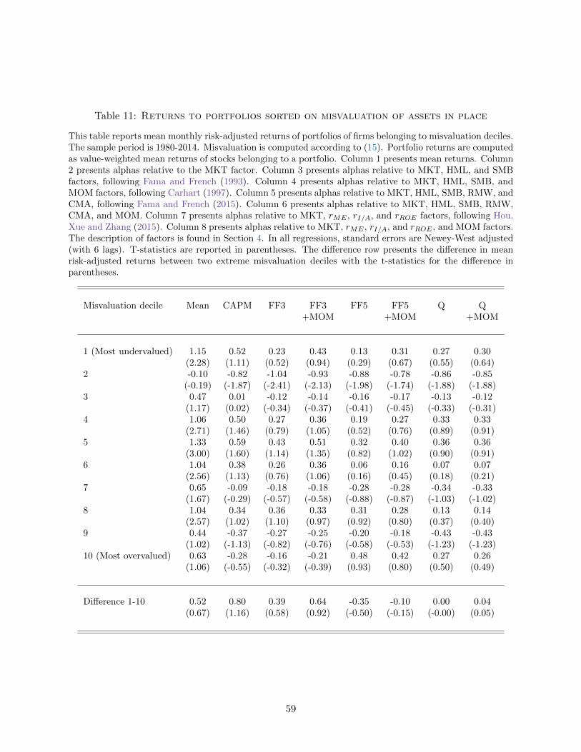
Table 11: Returns to portfolios sorted on misvaluation of assets in place

This table reports mean monthly risk-adjusted returns of portfolios of firms belonging to misvaluation deciles.The sample period is 1980-2014. Misvaluation is computed according to (15). Portfolio returns are computedas value-weighted mean returns of stocks belonging to a portfolio. Column 1 presents mean returns. Column2 presents alphas relative to the MKT factor. Column 3 presents alphas relative to MKT, HML, and SMBfactors, following Fama and French (1993). Column 4 presents alphas relative to MKT, HML, SMB, andMOM factors, following Carhart (1997). Column 5 presents alphas relative to MKT, HML, SMB, RMW, andCMA, following Fama and French (2015). Column 6 presents alphas relative to MKT, HML, SMB, RMW,CMA, and MOM. Column 7 presents alphas relative to MKT, rME , rI/A, and rROE factors, following Hou,Xue and Zhang (2015). Column 8 presents alphas relative to MKT, rME , rI/A, and rROE , and MOM factors.The description of factors is found in Section 4. In all regressions, standard errors are Newey-West adjusted(with 6 lags). T-statistics are reported in parentheses. The difference row presents the difference in meanrisk-adjusted returns between two extreme misvaluation deciles with the t-statistics for the difference inparentheses.

Misvaluation decile Mean CAPM FF3 FF3 FF5 FF5 Q Q+MOM +MOM +MOM

1 (Most undervalued) 1.15 0.52 0.23 0.43 0.13 0.31 0.27 0.30(2.28) (1.11) (0.52) (0.94) (0.29) (0.67) (0.55) (0.64)

2 -0.10 -0.82 -1.04 -0.93 -0.88 -0.78 -0.86 -0.85(-0.19) (-1.87) (-2.41) (-2.13) (-1.98) (-1.74) (-1.88) (-1.88)

3 0.47 0.01 -0.12 -0.14 -0.16 -0.17 -0.13 -0.12(1.17) (0.02) (-0.34) (-0.37) (-0.41) (-0.45) (-0.33) (-0.31)

4 1.06 0.50 0.27 0.36 0.19 0.27 0.33 0.33(2.71) (1.46) (0.79) (1.05) (0.52) (0.76) (0.89) (0.91)

5 1.33 0.59 0.43 0.51 0.32 0.40 0.36 0.36(3.00) (1.60) (1.14) (1.35) (0.82) (1.02) (0.90) (0.91)

6 1.04 0.38 0.26 0.36 0.06 0.16 0.07 0.07(2.56) (1.13) (0.76) (1.06) (0.16) (0.45) (0.18) (0.21)

7 0.65 -0.09 -0.18 -0.18 -0.28 -0.28 -0.34 -0.33(1.67) (-0.29) (-0.57) (-0.58) (-0.88) (-0.87) (-1.03) (-1.02)

8 1.04 0.34 0.36 0.33 0.31 0.28 0.13 0.14(2.57) (1.02) (1.10) (0.97) (0.92) (0.80) (0.37) (0.40)

9 0.44 -0.37 -0.27 -0.25 -0.20 -0.18 -0.43 -0.43(1.02) (-1.13) (-0.82) (-0.76) (-0.58) (-0.53) (-1.23) (-1.23)

10 (Most overvalued) 0.63 -0.28 -0.16 -0.21 0.48 0.42 0.27 0.26(1.06) (-0.55) (-0.32) (-0.39) (0.93) (0.80) (0.50) (0.49)

Difference 1-10 0.52 0.80 0.39 0.64 -0.35 -0.10 0.00 0.04(0.67) (1.16) (0.58) (0.92) (-0.50) (-0.15) (-0.00) (0.05)

59

Table 12: Excess returns in low and high sentiment environment

This table shows the performance of portfolios sorted on misvaluation (Panel A), and misvaluation andgrowth options (Panel B) during times of low and high sentiment. Sentiment is a non-orthogonalized indexof Baker and Wurgler (2006). Panel A reports value-weighted returns of portfolios of most undervalued(lowest misvaluation decile) and most overvalued (top misvaluation decile) stocks and the difference betweenthem in periods of low (below-median) and high (above-median) investor sentiment. Panel B reports value-weighted returns of UMO portfolios (i.e. the difference in returns of the most undervalued decile minus themost overvalued decile), constructed using high-growth-option firms (those with above-median measure ofgrowth options) and low-growth-option firms (those with below-median measure of growth options), duringtimes when our measure of investor sentiment is above and below median. The value of growth optionsis measured as either industry-median GO/AP ratio or industry-median M/B ratio. A firm’s GO/AP isthe ratio of a firm’s value of growth options (GO) to the value of its assets in place (AP). M/B is themarket-to-book ratio. Standard errors are Newey-West adjusted with 6 lags. t-statistics are reported inparentheses.

Panel A: Returns to portfolios sorted onsentiment and misvaluation

Misvaluation Mean CAPM FF3 FF3 FF5 FF5 Q Qdecile +MOM +MOM +MOM

Low sentiment

Most undervalued 1.21 0.36 0.34 0.44 0.46 0.52 0.69 0.64(2.89) (1.43) (1.38) (1.80) (1.84) (2.11) (2.70) (2.54)

Most overvalued 1.09 0.05 -0.03 -0.05 0.11 0.08 0.16 0.23(2.25) (0.21) (-0.11) (-0.22) (0.48) (0.35) (0.58) (0.86)

Difference 0.12 0.30 0.37 0.49 0.35 0.44 0.53 0.41(0.18) (0.85) (1.09) (1.46) (1.05) (1.32) (1.43) (1.13)

High sentiment

Most undervalued 0.97 0.64 1.07 1.20 1.16 1.27 1.39 1.39(1.80) (1.78) (2.96) (3.24) (3.13) (3.41) (3.78) (3.78)

Most overvalued -0.71 -1.12 -0.54 -0.55 -0.39 -0.43 -0.55 -0.55(-1.24) (-4.24) (-2.28) (-2.29) (-1.62) (-1.76) (-2.13) (-2.17)

Difference 1.68 1.76 1.61 1.75 1.55 1.70 1.94 1.94(2.13) (3.95) (3.73) (3.97) (3.51) (3.82) (4.32) (4.35)

60

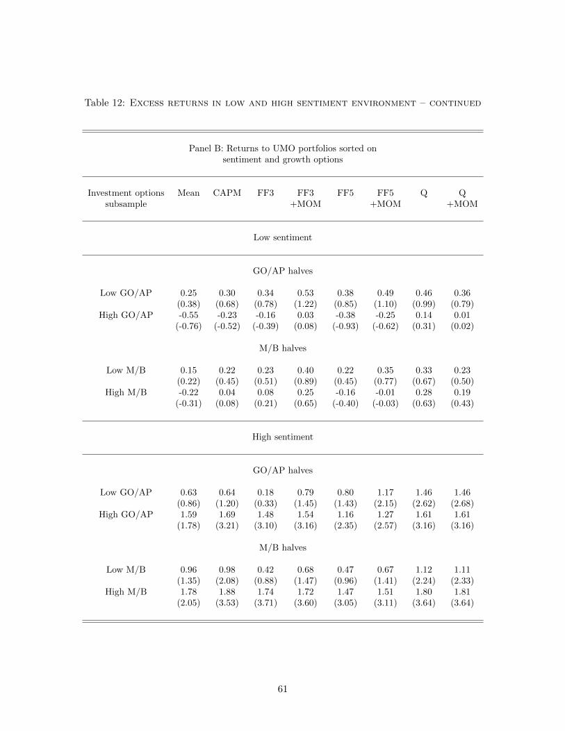
Table 12: Excess returns in low and high sentiment environment – continued

Panel B: Returns to UMO portfolios sorted onsentiment and growth options

Investment options Mean CAPM FF3 FF3 FF5 FF5 Q Qsubsample +MOM +MOM +MOM

Low sentiment

GO/AP halves

Low GO/AP 0.25 0.30 0.34 0.53 0.38 0.49 0.46 0.36(0.38) (0.68) (0.78) (1.22) (0.85) (1.10) (0.99) (0.79)

High GO/AP -0.55 -0.23 -0.16 0.03 -0.38 -0.25 0.14 0.01(-0.76) (-0.52) (-0.39) (0.08) (-0.93) (-0.62) (0.31) (0.02)

M/B halves

Low M/B 0.15 0.22 0.23 0.40 0.22 0.35 0.33 0.23(0.22) (0.45) (0.51) (0.89) (0.45) (0.77) (0.67) (0.50)

High M/B -0.22 0.04 0.08 0.25 -0.16 -0.01 0.28 0.19(-0.31) (0.08) (0.21) (0.65) (-0.40) (-0.03) (0.63) (0.43)

High sentiment

GO/AP halves

Low GO/AP 0.63 0.64 0.18 0.79 0.80 1.17 1.46 1.46(0.86) (1.20) (0.33) (1.45) (1.43) (2.15) (2.62) (2.68)

High GO/AP 1.59 1.69 1.48 1.54 1.16 1.27 1.61 1.61(1.78) (3.21) (3.10) (3.16) (2.35) (2.57) (3.16) (3.16)

M/B halves

Low M/B 0.96 0.98 0.42 0.68 0.47 0.67 1.12 1.11(1.35) (2.08) (0.88) (1.47) (0.96) (1.41) (2.24) (2.33)

High M/B 1.78 1.88 1.74 1.72 1.47 1.51 1.80 1.81(2.05) (3.53) (3.71) (3.60) (3.05) (3.11) (3.64) (3.64)

61

Table A1: Variable definitions

This table defines all variables used in the calibration, estimation, and empirical analysis. The main data sources areCompustat, CRSP, and IBES.

Variable Definition Source

Panel A: Variables used in calibration and estimation

Physical capital Gross property, plant and equipment (PP&E), item PPEGT. Compustat

Pre-tax operatingprofit

Earnings before interest, taxes, depreciation, and amortization (EBITDA),defined as SALE-COGS-XSGA.

Compustat

Drift of demandprocess

Estimated perpetual growth rate of demand in an industry. We start withforecasts of the long-term growth (LTG) rates issued by analysts and makevarious adjustments to it, discussed in Appendix C.

IBES, CRSP,Compustat

Volatility of demandprocess

Industry-median volatility of residuals of regressions of sales, item SALE, onquarterly dummies over 8 quarters.

Compustat

DepreciationIndustry median ratio of depreciation expense, DP, to lagged gross PP&E,item PPEGT.

Compustat

Panel B: Characteristics related to growth options

Industry M/B

Industry-median firm pseudo-M/B ratio, which is the ratio of the firm’spseudo-market value and its book assets. The firm’s pseudo-market value isthe sum of market value of equity, computed as the stock price, PRCC C,times the number of shares outstanding, CSHO, and book debt. Book debt isdefined as the difference between book assets, AT, and book value of equity.Book equity is stockholders’ equity, Compustat item TEQ, minus preferredstock plus balance sheet deferred taxes and investment tax credit, TXDITC,if available. If stockholders’ equity is missing, we use common equity pluspreferred stock par value, CEQ+PSTK. If these variables are missing, we usebook assets less liabilities, AT-(DLTT+DLC). Preferred stock is preferredstock liquidating value, PSTKRV, preferred stock redemption value, PSTKL,or preferred stock par value, PSTK, in that order of availability.

CRSP andCompustat

AgeThe difference between current year and the year of founding, the year ofincorporation, or the year the firm first appears in CRSP files, in that orderof availability.

CRSP andCompustat

R&D expenditures The ratio of R&D expenditures, XRD, to lagged assets, AT. Compustat

Asset growth The ratio of book assets, AT, and lagged book assets, minus one. Compustat

LeverageThe ratio of the sum of long-term debt, DLTT, and short-term debt, DLC,to book assets, AT.

Compustat

Equity betaEstimated using CAPM for the 60-month period preceding the month of theobservation.

CRSP

Standard deviationof returns

Computed using daily returns over a month preceding the month of theobservation.

CRSP

NASDAQ dummy Equals one if the stock exchange indicator, HEXCD, equals three. CSRP

62

Table A1: Variable definitions – continued

Variable Definition Source

Panel C: Characteristics used in cross-sectional tests

log (ME)The natural logarithm of the market value of equity. Market equity is definedas the stock price, PRCC C at the end of June preceding the month of theobservation, times the number of shares outstanding, CSHO.

CSRP

log (equity B/M)

The natural logarithm of the equity book-to-market ratio. Book equity isstockholders’ equity, TEQ, minus preferred stock plus balance sheet deferredtaxes and investment tax credit, TXDITC, if available. If stockholders’equity is missing, we use common equity plus preferred stock par value,CEQ+PSTK. If these variables are missing, we use book assets lessliabilities, AT-(DLTT+DLC). Preferred stock is preferred stock liquidatingvalue, PSTKRV, preferred stock redemption value, PSTKL, or preferredstock par value, PSTK, in that order of availability. Market equity is thestock price at the end of June, PRCC C,times the number of sharesoutstanding, CSHO. We match returns from January to June of year t withCompustat-based variables of year t− 2 , while the returns from July untilDecember are matched with Compustat variables of year t− 1.

CRSP andCompustat

InvestmentThe difference between gross property plant and equipment, PPEGT, and itslagged value, divided by lagged total assets, AT.

Compustat

ProfitabiltyThe difference between revenue, SALE, and cost of goods sold, COGS,divided by lagged total assets, AT.

Compustat

Return [-1,0) Return in month t− 1 prior to the month of the observation, t. CRSP

Return [-12,-1)Return over the 11-month period [t− 12, t− 2] prior to the month of theobservation, t.

CRSP

Panel D: Characteristics used in Rhodes-Kropf, Robinson and Viswanathan (2005) regressions

log (ME) Same as above. CRSP

log (BE)

The natural logarithm of the book value of equity. Book equity isstockholders’ equity, TEQ, minus preferred stock plus balance sheet deferredtaxes and investment tax credit, TXDITC, if available. If stockholders’equity is missing, we use common equity plus preferred stock par value,CEQ+PSTK. If these variables are missing, we use book assets lessliabilities, AT-(DLTT+DLC). Preferred stock is preferred stock liquidatingvalue, PSTKRV, preferred stock redemption value, PSTKL, or preferredstock par value, PSTK, in that order of availability.

Compustat

log (|NI|) The natural logarithm of the absolute value of net income, NI. Compustat

I(NI<0)The indicator variable that equals one if net income is below zero, and equalszero, otherwise.

Compustat

LeverageThe ratio of the sum of long-term debt, DLTT, and short-term debt, DLC,to book assets, AT.

Compustat

63

Table A1: Variable definitions – continued

Variable Definition Source

Panel E: Other characteristics

Assets Book assets, item AT. Compustat

Market value ofequity

Stock price, PRCC C, times the number of shares outstanding, CSHO. CRSP

Capital investmentThe difference between net PP&E, PPENT, and lagged PPENT, divided bylagged book assets, AT.

Compustat

Profitability The ratio of operating income after depreciation, OIADP, and sales, SALE. Compustat

Net issueThe difference between equity issues, SSTK, and repurchases, PRSTK,divided by lagged market value of equity, defined as above.

CRSP andCompustat

Amihud’s illiquiditymeasure

Monthly average of daily ratios of absolute return to dollar trading volume.Measured in dollars.

CRSP

Institutionalownership

The number of all shares held by institutions divided by total sharesoutstanding.

Number of analystsNumber of analysts that provide at least one forecast for the firm in theperiod [t− 3, t− 1] prior to the month of the observation, t.

IBES

Forecast dispersionCoefficient of variation of last forecast provided by each analyst in the period[t− 3, t− 1] prior to the month of the observation, t.

IBES

64

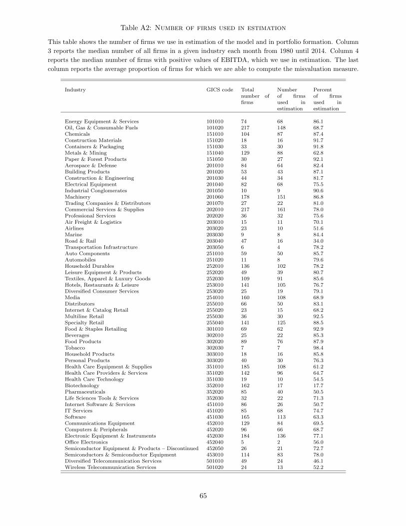
Table A2: Number of firms used in estimation

This table shows the number of firms we use in estimation of the model and in portfolio formation. Column

3 reports the median number of all firms in a given industry each month from 1980 until 2014. Column 4

reports the median number of firms with positive values of EBITDA, which we use in estimation. The last

column reports the average proportion of firms for which we are able to compute the misvaluation measure.

Industry GICS code Totalnumber offirms

Numberof firmsused inestimation

Percentof firmsused inestimation

Energy Equipment & Services 101010 74 68 86.1Oil, Gas & Consumable Fuels 101020 217 148 68.7Chemicals 151010 104 87 87.4Construction Materials 151020 18 16 91.7Containers & Packaging 151030 33 30 91.8Metals & Mining 151040 129 88 62.8Paper & Forest Products 151050 30 27 92.1Aerospace & Defense 201010 84 64 82.4Building Products 201020 53 43 87.1Construction & Engineering 201030 44 34 81.7Electrical Equipment 201040 82 68 75.5Industrial Conglomerates 201050 10 9 90.6Machinery 201060 178 151 86.8Trading Companies & Distributors 201070 27 22 81.0Commercial Services & Supplies 202010 217 161 78.0Professional Services 202020 36 32 75.6Air Freight & Logistics 203010 15 11 70.1Airlines 203020 23 10 51.6Marine 203030 9 8 84.4Road & Rail 203040 47 16 34.0Transportation Infrastructure 203050 6 4 78.2Auto Components 251010 59 50 85.7Automobiles 251020 11 8 79.6Household Durables 252010 136 102 78.2Leisure Equipment & Products 252020 49 39 80.7Textiles, Apparel & Luxury Goods 252030 109 91 85.6Hotels, Restaurants & Leisure 253010 141 105 76.7Diversified Consumer Services 253020 25 19 79.1Media 254010 160 108 68.9Distributors 255010 66 50 83.1Internet & Catalog Retail 255020 23 15 68.2Multiline Retail 255030 36 30 92.5Specialty Retail 255040 141 125 88.5Food & Staples Retailing 301010 69 62 92.9Beverages 302010 25 22 85.3Food Products 302020 89 76 87.9Tobacco 302030 7 7 98.4Household Products 303010 18 16 85.8Personal Products 303020 40 30 76.3Health Care Equipment & Supplies 351010 185 108 61.2Health Care Providers & Services 351020 142 96 64.7Health Care Technology 351030 19 10 54.5Biotechnology 352010 162 17 17.7Pharmaceuticals 352020 85 40 50.5Life Sciences Tools & Services 352030 32 22 71.3Internet Software & Services 451010 86 26 50.7IT Services 451020 85 68 74.7Software 451030 165 113 63.3Communications Equipment 452010 129 84 69.5Computers & Peripherals 452020 96 66 68.7Electronic Equipment & Instruments 452030 184 136 77.1Office Electronics 452040 5 2 56.0Semiconductor Equipment & Products – Discontinued 452050 26 21 72.7Semiconductors & Semiconductor Equipment 453010 114 83 78.0Diversified Telecommunication Services 501010 49 24 46.1Wireless Telecommunication Services 501020 24 13 52.2

65

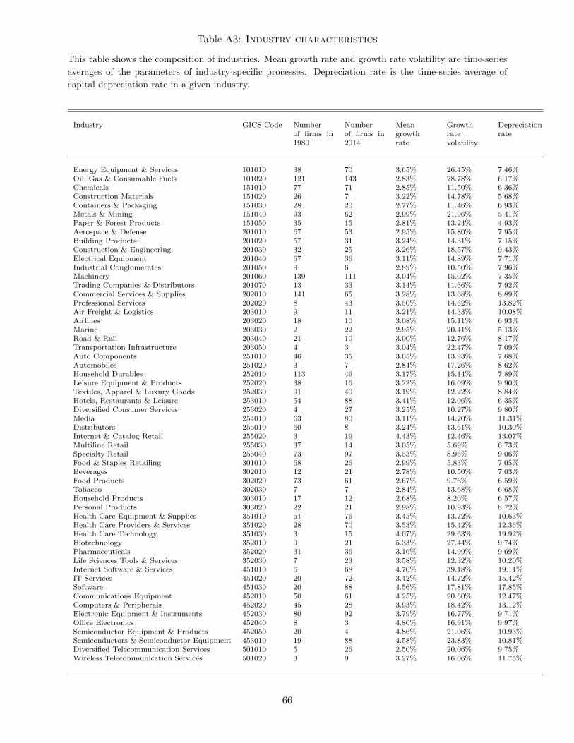
Table A3: Industry characteristics

This table shows the composition of industries. Mean growth rate and growth rate volatility are time-series

averages of the parameters of industry-specific processes. Depreciation rate is the time-series average of

capital depreciation rate in a given industry.

Industry GICS Code Numberof firms in1980

Numberof firms in2014

Meangrowthrate

Growthratevolatility

Depreciationrate

Energy Equipment & Services 101010 38 70 3.65% 26.45% 7.46%Oil, Gas & Consumable Fuels 101020 121 143 2.83% 28.78% 6.17%Chemicals 151010 77 71 2.85% 11.50% 6.36%Construction Materials 151020 26 7 3.22% 14.78% 5.68%Containers & Packaging 151030 28 20 2.77% 11.46% 6.93%Metals & Mining 151040 93 62 2.99% 21.96% 5.41%Paper & Forest Products 151050 35 15 2.81% 13.24% 4.93%Aerospace & Defense 201010 67 53 2.95% 15.80% 7.95%Building Products 201020 57 31 3.24% 14.31% 7.15%Construction & Engineering 201030 32 25 3.26% 18.57% 9.43%Electrical Equipment 201040 67 36 3.11% 14.89% 7.71%Industrial Conglomerates 201050 9 6 2.89% 10.50% 7.96%Machinery 201060 139 111 3.04% 15.02% 7.35%Trading Companies & Distributors 201070 13 33 3.14% 11.66% 7.92%Commercial Services & Supplies 202010 141 65 3.28% 13.68% 8.89%Professional Services 202020 8 43 3.50% 14.62% 13.82%Air Freight & Logistics 203010 9 11 3.21% 14.33% 10.08%Airlines 203020 18 10 3.08% 15.11% 6.93%Marine 203030 2 22 2.95% 20.41% 5.13%Road & Rail 203040 21 10 3.00% 12.76% 8.17%Transportation Infrastructure 203050 4 3 3.04% 22.47% 7.09%Auto Components 251010 46 35 3.05% 13.93% 7.68%Automobiles 251020 3 7 2.84% 17.26% 8.62%Household Durables 252010 113 49 3.17% 15.14% 7.89%Leisure Equipment & Products 252020 38 16 3.22% 16.09% 9.90%Textiles, Apparel & Luxury Goods 252030 91 40 3.19% 12.22% 8.84%Hotels, Restaurants & Leisure 253010 54 88 3.41% 12.06% 6.35%Diversified Consumer Services 253020 4 27 3.25% 10.27% 9.80%Media 254010 63 80 3.11% 14.20% 11.31%Distributors 255010 60 8 3.24% 13.61% 10.30%Internet & Catalog Retail 255020 3 19 4.43% 12.46% 13.07%Multiline Retail 255030 37 14 3.05% 5.69% 6.73%Specialty Retail 255040 73 97 3.53% 8.95% 9.06%Food & Staples Retailing 301010 68 26 2.99% 5.83% 7.05%Beverages 302010 12 21 2.78% 10.50% 7.03%Food Products 302020 73 61 2.67% 9.76% 6.59%Tobacco 302030 7 7 2.84% 13.68% 6.68%Household Products 303010 17 12 2.68% 8.20% 6.57%Personal Products 303020 22 21 2.98% 10.93% 8.72%Health Care Equipment & Supplies 351010 51 76 3.45% 13.72% 10.63%Health Care Providers & Services 351020 28 70 3.53% 15.42% 12.36%Health Care Technology 351030 3 15 4.07% 29.63% 19.92%Biotechnology 352010 9 21 5.33% 27.44% 9.74%Pharmaceuticals 352020 31 36 3.16% 14.99% 9.69%Life Sciences Tools & Services 352030 7 23 3.58% 12.32% 10.20%Internet Software & Services 451010 6 68 4.70% 39.18% 19.11%IT Services 451020 20 72 3.42% 14.72% 15.42%Software 451030 20 88 4.56% 17.81% 17.85%Communications Equipment 452010 50 61 4.25% 20.60% 12.47%Computers & Peripherals 452020 45 28 3.93% 18.42% 13.12%Electronic Equipment & Instruments 452030 80 92 3.79% 16.77% 9.71%Office Electronics 452040 8 3 4.80% 16.91% 9.97%Semiconductor Equipment & Products 452050 20 4 4.86% 21.06% 10.93%Semiconductors & Semiconductor Equipment 453010 19 88 4.58% 23.83% 10.81%Diversified Telecommunication Services 501010 5 26 2.50% 20.06% 9.75%Wireless Telecommunication Services 501020 3 9 3.27% 16.06% 11.75%

66

Table A4: Persistence of estimated parameters θ and η

This table reports means of absolute changes in the estimated curvature of the production function, θ, andthe cost of purchasing and installing new capital, η, at 1-month, 3-month, 6-month, 1-year, 2-year, and3-year horizons. The means are pooled across industries and across months. Column 2 shows the mean ofabsolute changes in θ at the same horizons. Column 3 reports the mean of absolute changes in η. The lasttwo columns report the ratios of absolute changes in θ and η respectively, and their corresponding meanvalues.

Lag Absolute Absolute Percentage absolute Percentage absolutechange in θ change in η change in θ change in η

1 0.015 0.027 4.8% 2.3%3 0.030 0.050 9.5% 4.3%6 0.046 0.076 14.4% 6.5%12 0.067 0.111 21.0% 9.4%24 0.087 0.148 27.0% 12.6%36 0.090 0.163 28.3% 13.8%

67