The Valuation Accuracy of Multiples in Mergers and

Acquisitions, and their association with Firm Misvaluation

by

Michel Bradley Stubbs

Bachelor of Business

Principal Supervisor: Professor Gerry Gallery

A thesis submitted in fulfilment of the requirements for the degree of

Master of Business (Research)

to the

School of Accountancy

Queensland University of Technology

2012

ii

iii

ACKNOWLEDGEMENTS

I am grateful for many people who have assisted me with support, encouragement

and feedback as I have undertaken this thesis.

I am especially grateful for my principal supervisor, Professor Gerry Gallery. I

appreciated his guidance, feedback and patience along this journey.

I appreciate the funding provided by the School of Accountancy and Queensland

University of Technology.

I am also grateful for the staff and fellow students at Queensland University of

Technology, family and friends for their support during this time.

STATEMENT OF ORIGINAL AUTHORSHIP

"The work contained in this thesis has not been previously submitted to meet requirements for an award at this or any other higher education institution. To the best of my knowledge and belief, the thesis contains no material previously published or written by another person except where due reference is made."

Signature

Date

iv

QUT Verified Signature

v

ABSTRACT

This study explores the accuracy and valuation implications of the application of a

comprehensive list of equity multiples in the takeover context. Motivating the study

is the prevalent use of equity multiples in practice, the observed long-run

underperformance of acquirers following takeovers, and the scarcity of multiples-

based research in the merger and acquisition setting. In exploring the application of

equity multiples in this context three research questions are addressed: (1) how

accurate are equity multiples (RQ1); which equity multiples are more accurate in

valuing the firm (RQ2); and which equity multiples are associated with greater

misvaluation of the firm (RQ3).

Following a comprehensive review of the extant multiples-based literature it is

hypothesised that the accuracy of multiples in estimating stock market prices in the

takeover context will rank as follows (from best to worst): (1) forecasted earnings

multiples, (2) multiples closer to bottom line earnings, (3) multiples based on Net

Cash Flow from Operations (NCFO) and trading revenue. The relative inaccuracies

in multiples are expected to flow through to equity misvaluation (as measured by the

ratio of estimated market capitalisation to residual income value, or P/V).

Accordingly, it is hypothesised that greater overvaluation will be exhibited for

multiples based on Trading Revenue, NCFO, Book Value (BV) and earnings before

interest, tax, depreciation and amortisation (EBITDA) versus multiples based on

bottom line earnings; and that multiples based on Intrinsic Value will display the

least overvaluation.

The hypotheses are tested using a sample of 147 acquirers and 129 targets involved

in Australian takeover transactions announced between 1990 and 2005. The results

show that first, the majority of computed multiples examined exhibit valuation errors

within 30 percent of stock market values. Second, and consistent with expectations,

the results provide support for the superiority of multiples based on forecasted

earnings in valuing targets and acquirers engaged in takeover transactions. Although

a gradual improvement in estimating stock market values is not entirely evident

vi

when moving down the Income Statement, historical earnings multiples perform

better than multiples based on Trading Revenue or NCFO. Third, while multiples

based on forecasted earnings have the highest valuation accuracy they, along with

Trading Revenue multiples for targets, produce the most overvalued valuations for

acquirers and targets. Consistent with predictions, greater overvaluation is exhibited

for multiples based on Trading Revenue for targets, and NCFO and EBITDA for

both acquirers and targets. Finally, as expected, multiples based Intrinsic Value

(along with BV) are associated with the least overvaluation.

Given the widespread usage of valuation multiples in takeover contexts these

findings offer a unique insight into their relative effectiveness. Importantly, the

findings add to the growing body of valuation accuracy literature, especially within

Australia, and should assist market participants to better understand the relative

accuracy and misvaluation consequences of various equity multiples used in takeover

documentation and assist them in subsequent investment decision making.

KEYWORDS: Takeovers, mergers and acquisitions, multiples, takeover

misvaluation, acquirer and target valuation, valuation accuracy, residual income

valuation.

vii

TABLE OF CONTENTS

Page

ACKNOWLEDGEMENTS iii STATEMENT OF ORIGINAL AUTHORSHIP iv ABSTRACT v

LIST OF TABLES ix LIST OF ABBREVIATIONS x CHAPTER 1 INTRODUCTION 1

1.1 Study Overview 1 1.2 Background to Multiples 1

1.3 Motivation 3

1.4 Research Questions and Hypotheses 6

1.5 Research Design 7 1.6 Main Results 7 1.7 Contribution 9 1.8 Structure of Thesis 9

CHAPTER 2 LITERATURE REVIEW 10 2.1 Overview 10 2.2 Research on Long-run Underperformance Following Takeovers 10

2.2.1 Long-run Underperformance of Acquirers 10 2.2.2 Possible Reasons for Long-run Underperformance 14

2.2.3 Evaluation of Underperformance Reasons and Valuation

Implications 20 2.3 Valuation Accuracy of Multiples 20

2.3.1 Transaction Valuations Methods using Multiples 20

2.3.2 Accuracy of Multiples Based on Various Value Drivers 22 2.3.3 Factors Explaining the Variation in Accuracy of Multiple-

Based Valuation Methods 28

2.4 Conclusion 30 CHAPTER 3 HYPOTHESES DEVELOPMENT 33

3.1 Introduction 33 3.2 Valuation Accuracy of Multiples (RQ1 & 2) 33 3.3 Misvaluation of Takeover Firms Using Various Multiples to

Estimate Market Capitalisation (P) in P/V Ratios (RQ3) 36 3.4 Conclusion 43

CHAPTER 4 RESEARCH DESIGN 45

4.1 Introduction 45

4.2 Sampling Procedure and Data Sources 45 4.3 Valuation Accuracy of Multiples 48

4.3.1 Valuation Accuracy Model 48 4.3.2 Value Drivers 50 4.3.3 Comparable Firms 50

4.4 Estimation Procedure for Misvaluation Proxy (P/V) 51 4.5 Limitation of the Research Design 53 4.6 Conclusion 53

CHAPTER 5 RESULTS 55 5.1 Introduction 55 5.2 Descriptive Statistics 55

viii

5.3 Valuation Accuracy of Multiples Results 55

5.3.1 Valuation Accuracy of Multiples Based Valuations in General

(RQ1) 56 5.3.2 Valuation Accuracy of Various Multiples Based Valuations

(RQ2) 62 5.3.3 Summary of Findings for Hypotheses H1a-c 65

5.4 Misvaluation Results (RQ3) 66 5.4.1 Misvaluation Hypothesis Testing (Hypotheses H2a – H2c) 67 5.4.2 Summary of findings for Hypotheses H2a-c 74

5.5 Conclusion 75 CHAPTER 6 SENSITIVITY ANALYSIS 79

6.1 Introduction 79 6.2 Historical Value Driver Results 79

6.2.1 Historical Absolute Valuation Accuracy of Multiples 80 6.2.2 P/V ratios of Historical Value Drivers 81

6.3 Matched Acquirer and Target Results 83

6.3.1 Matched Acquirers and Targets Absolute Valuation Errors 84 6.3.2 Matched Acquirers and Targets P/V Ratios 84

6.4 Future Market Capitalisation Results 85 6.4.1 Future Market Capitalisation Valuation Accuracy 86

6.5 Conclusion 87 CHAPTER 7 CONCLUSION 89

7.1 Summary 89 7.2 Discussion of Findings 92 7.3 Limitations of Study 93

7.4 Future Research 94

7.5 Contribution 95 REFERENCES 97 APPENDIX A 107

APPENDIX B 112 APPENDIX C 113

APPENDIX D 114

ix

LIST OF TABLES

Page

Table 1.1 Example of an Application of Multiples in an Takeover Setting 3 Table 2.1 Summary of the Key Multiples-based Valuation Studies 32 Table 4.1 Sample Size Selection 47

Table 5.1 Distribution of Value Drivers 58 Table 5.2 Absolute Valuation Errors 60 Table 5.3 Signed Valuation Errors 68 Table 5.4 Price to Intrinsic Value (P/V) Ratios 70 Table 5.5 Summary of Hypotheses and Results 76

Table B.1 Morningstar FinAnalysis Financial Items Description 112 Table C.1 Description of Multiples 113

Table D.1 Absolute Valuation Errors for Historical Value Drivers 114 Table D.2 Signed Valuation Errors for Historical Value Drivers 116 Table D.3 Price to Intrinsic Value (P/V) Ratios for Historical Value Drivers 118 Table D.4 Matched Absolute Valuation Errors 120

Table D.5 Matched Signed Valuation Errors 122 Table D.6 Matched Price to Intrinsic Value (P/V) Ratios 124 Table D.7 Acquirers Absolute Valuation Errors Using One Year Ahead Market

Capitalisation 126 Table D.8 Acquirers Absolute Valuation Errors Using Two Year Ahead Market

Capitalisation 127 Table D.9 Acquirers Absolute Valuation Errors Using Three Year Ahead Market

Capitalisation 128

x

LIST OF ABBREVIATIONS

ASX Australian Stock Exchange

B/P Book-to-price

BV Book Value

CAAR Cumulative average abnormal returns

CAPM Capital asset pricing model

CEO Chief Executive Officer

DCF Discounted cash flow

EBIT Earnings before interest and tax

EBITA Earnings before interest, tax and amortisation

EBITD Earnings before interest, tax and depreciation

EBITDA Earnings before interest, tax, depreciation and amortisation

EBO Edwards-Bell-Ohlson

EBT Earnings before tax

EPS Earnings-per-share

EV Enterprise value

FEPS1 Analyst forecasts of EPS for one year ahead

FEPS2 Analyst forecasts of EPS for two years ahead

FROE Forecasted return on equity

GAAP Generally Accepted Accounting Principles

GICS Global Industry Classification Standard

I/B/E/S Institutional Brokers’ Estimate System

IPO Initial public offer

IV Intrinsic Value

MAM Market adjusted model

NAICS North American Industry Classification System

NCFO Net cash flow from operations

NPAT Net profit after tax

P/B Price-to-book

P/E Price-to-earnings

P/V Price-to-intrinsic value

PEG Price/earnings-to-growth

RIM Residual income model

ROE Return on equity

SIC Standard Industrial Classification

SPPR Share price and price relative

V/P Value-to-price

1

CHAPTER 1 INTRODUCTION

1.1 Study Overview

For over a century investors, managers and academics have sought to determine

whether takeovers generate shareholder wealth. This question also has had renewed

meaning due to the ongoing uncertainty in global financial markets, and

unprecedented heights of global merger and acquisition deal value coupled with

prominent takeover failures in the lead up to the global financial crisis. These market

conditions motivate continued effort to identify factors that contribute to wealth

creation or destruction as a result of mergers and acquisitions.

Takeover literature suggests one important contributing factor to wealth destruction

is misvaluation of the target and/or acquirer. Multiples are frequently employed in

the valuations decisions in takeover contexts. Thus, incorrect application of multiples

is likely to be a contributing factor in misvaluation outcomes.

As there is little known research the objective of this thesis is to examine the

application, accuracy and valuation implications of common multiples used in the

takeover context. By considering multiples in this context, the study combines two

important streams of research: the valuation accuracy of multiples and the

misvaluation of firms prior to a takeover. Specifically, this study seeks to investigate

the performance of various multiples used in valuing target and acquirer firms.

1.2 Background to Multiples

Multiples are used in practice to value a particular company based on the comparable

value of similar firms. The conceptual strengths of multiples include their simplicity

of application as well as understandability. Multiples generally reflect the current

disposition of the market, and are available in the financial press. Lastly, multiples

are a communication tool of sell-side analysts and allow fundamental screening.

However multiples are not without their weaknesses. Their simplicity is due to the

intrinsic assumptions made. Thus, by their nature multiples are limited due to their

2

short-sightedness, and are affected by market bubbles (and conversely, recessions).

Multiples are also susceptible to a manager’s accounting method choices and

earnings management activities. Multiples based on earnings and cash flow are the

most commonly used, with some multiples alternately using book value (BV) or

revenue.

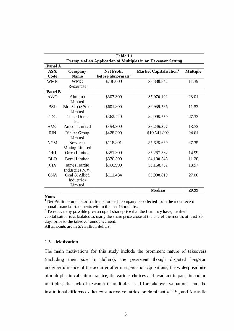
Mathematically, the value of a firm could be estimated by multiplying a value driver

(such as Net Profit before abnormal items) by a corresponding multiple, where the

multiple is derived from the ratio of market capitalisation to that value driver for a

group of comparable firms. This is demonstrated in an example below and in Table

1.1.

On 8 March 2005 BHP Billiton announced a U.S.$7.27 billion (A$9.17 billion)

friendly takeover bid of WMC Resources (Australian Financial Review, 2005). For

illustrative purposes to show how to value a company with multiples, 10 Australian

listed companies with the closest market capitalisation (end of the month, at least 30

days prior to the takeover announcement) and from the same industry (Materials) to

WMC Resources are shown below. Their Net Profit before abnormal items from the

most recent financial statements as well as their respective market capitalisation are

also included.

Using multiples, the value of WMC Resources could be calculated by multiplying its

Net Profit before abnormal items (A$736 million) by the median multiple of the

comparable firms (20.99). This gives WMC Resources an estimated market value of

A$15.45 billion (excluding a takeover premium). Alternatively, using every

Australian listed company within the same industry (excluding WMC Resources and

BHP Billiton) would give a median multiple of 15.12 for the 119 remaining firms.

This would therefore give an estimated market value of WMC Resources of A$11.13

billion (also excluding a takeover premium). This example highlights both the

simplicity of an application of a multiples-based valuation method and the

differences that can result from the choice of comparative companies.

3

Table 1.1

Example of an Application of Multiples in an Takeover Setting

Panel A

ASX

Code

Company

Name

Net Profit

before abnormals1

Market Capitalisation2

Multiple

WMR WMC

Resources

$736.000 $8,380.842 11.39

Panel B

AWC Alumina

Limited

$307.300 $7,070.101 23.01

BSL BlueScope Steel

Limited

$601.800 $6,939.786 11.53

PDG Placer Dome

Inc.

$362.440 $9,905.750 27.33

AMC Amcor Limited $454.800 $6,246.397 13.73

RIN Rinker Group

Limited

$428.300 $10,541.802 24.61

NCM Newcrest

Mining Limited

$118.801 $5,625.639 47.35

ORI Orica Limited $351.300 $5,267.362 14.99

BLD Boral Limited $370.500 $4,180.545 11.28

JHX James Hardie

Industries N.V.

$166.999 $3,168.752 18.97

CNA Coal & Allied

Industries

Limited

$111.434 $3,008.819 27.00

Median 20.99

Notes 1 Net Profit before abnormal items for each company is collected from the most recent

annual financial statements within the last 18 months. 2 To reduce any possible pre-run up of share price that the firm may have, market

capitalisation is calculated as using the share price close at the end of the month, at least 30

days prior to the takeover announcement.

All amounts are in $A million dollars.

1.3 Motivation

The main motivations for this study include the prominent nature of takeovers

(including their size in dollars); the persistent though disputed long-run

underperformance of the acquirer after mergers and acquisitions; the widespread use

of multiples in valuation practice; the various choices and resultant impacts in and on

multiples; the lack of research in multiples used for takeover valuations; and the

institutional differences that exist across countries, predominantly U.S., and Australia

4

that may contribute to differences in valuation approaches and post acquisition

performance.

Mergers and acquisitions involve the exchange of millions or even billions of dollars

worth of value. In 2006, total global merger and acquisition deal values reached an

unprecedented amount of U.S. $3.79 trillion (KPMG and Kaplan, 2007). During the

same period, Australia experienced mergers and acquisitions totalling A$67 billion,

with deals of A$133 billion the following year (2007) (KPMG, 2008). Such activities

also have consequences to other interested parties, such as employees, suppliers,

customers, regulators, creditors and shareholders. More recently, global merger and

acquisition deals for 2010 totalled U.S.$2.18 trillion (Mergermarket, 2011).

It is puzzling why so many mergers and acquisitions occur when academic research

finds combined entities underperform for up to five years following a takeover (for

example, see Agrawal, Jaffe, & Mandelker, 1992; Brown, Dong, & Gallery, 2005;

Martynova & Renneboog, 2008). Apart from possible measurement issues, many

reasons have been suggested for this long-run underperformance, including

overconfidence of managers (over extrapolation or managerial hubris) (Rau &

Vermaelen 1998; Roll 1986); method of payment (Travlos, 1987); and management

and market fixation on earnings-per-share (EPS) myopia (Lys & Vincent, 1995).

Takeover waves generally occur during times of soaring (hot) equity markets and

times of rapid credit expansion (Martynova and Renneboog, 2008). Several studies

have documented the misvaluation of firms at the time of the takeover, including

Brown et al. (2005) and Dong, Hirshleifer, Richardson and Teoh (2006), with

Rhodes-Kropf, Robinson and Viswanathan (2005) finding more acquisitions occur

when an industry is overvalued, with the majority of these acquisitions undertaken by

acquirers with the highest overvaluation. This is consistent with both Schleifer and

Vishney (2003) and Rhodes-Kropf and Viswanathan (2004) models of mergers and

acquisitions where acquirers of overvalued firms take advantage of windows of

opportunities presented by market inefficiencies.

There are numerous ways to value a company, including discounted cash flow

models, residual income models, and valuations based on comparable companies and

5

transactions. Valuations based on multiples are used quite frequently in practice,

especially in analysts’ reports, Australian independent expert reports, and investment

bankers’ U.S. fairness opinions. Asquith, Mikhail and Au (2005) reveal that 99

percent of top analysts use a multiple for firm valuation in their analyst reports. In his

survey of European institutional equity analysts Fernandez (2001) finds that price-to-

earnings (P/E) and enterprise value to earnings before interest, tax, depreciation and

amortisation (EV/EBITDA) multiples are more commonly used than more complex

and theoretically sound valuation tools such as the discounted cash flow method and

the residual income model. Similarly, Demirakos, Strong and Walker (2004) study

the valuation methodologies contained in 104 analysts’ reports for international

investment bankers for 26 large U.K. listed companies drawn from selected

industries and find that 88 percent of reports surveyed contained some reference to a

multiple of earnings. Barker (1999) and Bradshaw (2002) also find similar results for

the general use of P/E multiples in practice. In the takeover context, Damodaran

(2002) comments that approximately 90 percent of equity research valuations and 50

percent of acquisition valuations are based on multiples.

Valuations using multiples, as in any valuation method, involve choosing from a

menu of alternatives. Specifically, what is being valued (Finnerty & Emery, 2004;

Kaplan & Ruback, 1995), the choice of value driver (Liu, Nissim, & Thomas, 2002;

Schreiner & Spremann, 2007), using trailing or forward values (Kim & Ritter, 1999,

Lie & Lie, 2002), and the selection of the set of comparable firms (Alford, 1992;

Bhojraj & Lee, 2002) are amongst the choices to be made in valuing companies

involved in mergers and acquisitions. All have influence on the valuation accuracy of

a particular multiple. Additionally, both Schreiner and Spremann (2007) and

Henschke and Homburg (2009) observe the valuation accuracy of multiples declined

in years leading up to and including 2000, and subsequently improved, both

associated with the dot-com boom and bust.

Very few published (U.S.) studies have investigated the valuation accuracy of

multiples in takeovers (Finnerty & Emery, 2004; Kaplan & Ruback, 1995). These

U.S. studies may or may not apply to a non-U.S. context, namely Australia.

Institutional differences, notably the relative size of U.S. companies to those of their

Australian counterparts, suggest that research in the Australian market may be

6

warranted. In terms of market capitalisation, many U.S. studies have involved only

medium to large sized firms (for example Liu et al. 2002; Schreiner & Spremann,

2007). Australia by its very nature is much smaller in terms of market capitalisation.

There are also accounting differences that may cause differences in valuation

accuracy in comparison to the U.S., with Australia having adopted international

accounting standards in contrast to the U.S. Generally Accepted Accounting

Principles (GAAP). Furthermore, there have traditionally been differences in the

treatment of significant or unusual items. These differences in accounting and market

size warrant study into a market outside the U.S. Therefore, given the widespread use

of multiples in the valuation practice, this warrants further research into the valuation

accuracy of such measures, and their association with long-run underperformance in

the Australian context.

In summary, there are many motivations for this study, including the prominent

nature of takeovers (including their size in dollars); the persistent though disputed

long-run underperformance of the acquirer after mergers and acquisitions; the

widespread use of multiples in valuation practice, and the varied choices and

resultant impacts in and on such multiples; the lack of research in multiples used for

takeover valuations; and the institutional differences between other countries’

studies, predominantly the U.S. and Australia.

1.4 Research Questions and Hypotheses

Given the prevalent use of multiples in practice, and the limitations in existing

literature, this study examines the following research questions:

1. How accurate are various multiple-based valuation methods in valuing firms

involved in mergers and acquisitions?

2. Which of the various multiple-based valuation methods are more accurate in

valuing target and acquirer firms involved in takeovers?

3. Which of the various multiple-based valuation methods is associated with

greater misvaluation (as measured by higher estimations of Price-to-Intrinsic

Value)?

7

Based on the prior literature on multiples in various contexts and merger and

acquisition research, testable hypotheses are developed to address RQ2 and RQ3. In

terms of valuation accuracy, these hypotheses predicted that value drivers based on

forecasted earnings will have lower valuation errors than those based on historical

value drivers (H1a); that value drivers closer to bottom line earnings (Net income)

have lower valuation errors than those closer to the Trading Revenue income

statement line (H1b); and that value drivers based on earnings (excluding Trading

Revenue) have lower valuation errors than those based on net cash flow from

operations (NCFO) (H1c). In terms of misvaluation, these hypotheses predicted that

estimations of P/V ratios using forecasted earnings multiples are closer to P/V ratios

based on actual market capitalisation (H2a); that estimations of P/V ratios based on

bottom line earnings (net income) are lower than those based on Trading Revenue,

NCFO, BV and EBITDA multiples (H2b); and that estimations of P/V ratios based

on Intrinsic Value multiples are lower than those based on earnings or cash flow

based multiples.

1.5 Research Design

This study examines 147 acquirers and 129 targets involved in takeovers

announcements from 1 January 1990 to 31 December 2005. Valuation analysis is

used to investigate how accurate various multiple-based valuation methods are in

valuing firms involved in mergers and acquisitions, as well as to determine which of

the various multiple-based valuation methods are the most accurate. This is then

followed by calculating a P/V ratio, where price is estimated using the various value

drivers, and Intrinsic Value calculated from a residual income model. P/V ratios are

then used to ascertain which multiple-based valuation methods are associated with

greater misvaluation, with higher P/V ratios suggesting greater over-valuation.

1.6 Main Results

The major findings in this thesis are: first, the majority of computed multiples

examined exhibit valuation errors within 30 percent of stock market values. Second,

and consistent with expectations, from a valuation accuracy point of view the results

provide support for the superiority of multiples based on forecasted earnings in

8

valuing targets and acquirers engaged in takeover transactions. Although a gradual

improvement in estimating stock market values is not entirely evident when moving

down the Income Statement, historical earnings multiples perform better than

multiples based on Trading Revenue or NCFO. Third, while multiples based on

forecasted earnings have the highest valuation accuracy they, along with Trading

Revenue multiples for targets, produce the most overvalued valuations for acquirers

and targets. Consistent with predictions, greater overvaluation is exhibited for

multiples based on Trading Revenue for targets, and NCFO and EBITDA for both

acquirers and targets. Finally, as expected, multiples based Intrinsic Value (along

with BV) are associated with the least overvaluation.

These findings are predominantly robust to the alternative conditions examined in the

sensitivity analysis, namely: increasing of the sample size by removing the

requirement for analysts’ forecasts; reducing the sample size by investigating

acquirers and targets where both meet the requirements to have sufficient

information and comparable firms; and using one, two and three ahead stock market

values as a benchmark for valuation analysis. Nevertheless, three notable insights

from the sensitivity analyses were observed. First, target firms’ valuation accuracy

decreases with the inclusion of firms that are not followed by analyst forecasts

(generally smaller and less profitable firms); Second, the valuation accuracy of an

acquirer multiple diminishes over time when using one, two and three year ahead

market capitalisation as a benchmark. Specifically, the supremacy of forecasted

earnings multiples diminishes significantly when using two year ahead market

capitalisation as a benchmark, with the EBT multiple displaying the same amount of

valuation accuracy. This result suggests the predictive power of forecasted earnings

is most prevalent for current and one year ahead stock market capitalisation.

Similarly, the range of valuation accuracy between the multiples declines as the

benchmark projects into the future. Third, the stock market price at the time of the

takeover announcement has higher valuation accuracy against one, two and three

year ahead market capitalisation than all multiples examined, including forecasted

earnings.

9

1.7 Contribution

This study contributes to prior literature and will be helpful for those using valuation

multiples in practice. First, it is the first known study to examine the valuation

accuracy of a range of multiples for a much studied subset of companies; those

involved in mergers and acquisitions. Second, this study provides the link between

two bodies of literature, namely valuation accuracy of certain multiples and their

relation to company misvaluation. Lastly, the study’s findings have ramifications for

the users of multiples in practice. These users include not only investment bankers

who use these multiples in independent expert reports, but also the shareholders and

managers of both acquirers and targets, and hence firms’ employees, customers,

creditors and regulators.

1.8 Structure of Thesis

The thesis is structured as follows. Chapter 2 reviews the body of literature for both

the long-run underperformance of bidders subsequent to a takeover announcement,

and the valuation accuracy of various multiples. Chapter 3 provides the rational

between the link between valuation accuracy and misvaluation (as measured by P/V

ratio), as well as outlining the research questions and hypotheses for this study.

Chapter 4 describes the research design involved in testing the research questions

and hypotheses. Chapter 5 enumerates the results to the research questions and

hypotheses, with Chapter 6 providing further insights through sensitivity analysis.

This study then concludes in Chapter 7 with a discussion of the main findings,

contributions and implications of the study’s findings.

10

CHAPTER 2 LITERATURE REVIEW

2.1 Overview

As outlined in Chapter 1 and in the context of mergers and acquisitions, the three

research questions addressed by this study are: (1) how accurate are equity multiples;

(2) which equity multiples are more accurate in valuing firms; and (3) which equity

multiples are associated with greater misvaluation. This chapter reviews the prior

literature related to these three questions. First, establishing the merger and

acquisition context, this study examines the acquirers’ long-run underperformance

literature, summarising the various hypotheses for this anomaly including

misvaluation. Second, as multiples are prevalent in valuing firms, this study reviews

the valuation accuracy of multiples literature. The chapter concludes by highlighting

gaps in the valuation accuracy literature.

2.2 Research on Long-run Underperformance Following Takeovers

2.2.1 Long-run Underperformance of Acquirers

In this section, major studies into the long-run underperformers of acquirers, both

within the U.S., other countries, and then specifically Australia are reviewed.

Studies examining the effect of takeover characteristics on long-run

underperformance will then be discussed. An event study approach is the most

common method employed in these studies to assess the long-term shareholder

wealth effects of mergers and acquisitions. This approach involves calculating

abnormal returns: the difference between realised returns, and an expected or

benchmark return based on a market index, or a comparable firm not involved in a

takeover.

U.S. and International Studies

Jensen and Ruback (1983) review the literature of the long-run performance of

acquirers following a takeover, and find that acquirers experience statistically

insignificant positive abnormal returns after a tender offer, compared to acquirers

that systematically underperform following a merger. However studies around this

11

time and afterwards find mixed results for the long-run underperformance of

acquirers. For example, Langetieg (1978), Bradley and Jarrell (1988) and Franks,

Harris and Titman (1991) do not find significant underperformance of acquirers in

the two to three years following the acquisition. Mitchell and Stafford (2000) and

Andrade, Mitchell and Stafford (2001), also find acquirers experience lower absolute

value long-run returns which are statistically insignificant.

In contrast, Asquith (1983) and Agrawal, Jaffe and Mandelker (1992) document

significant negative returns experienced by acquirers for a couple of years following

a merger. Specifically, Agrawal et al. (1992) examine the long-run underperformance

of acquiring firms of 765 mergers offers between 1955 and 1987 in the U.S., where

the acquirer was listed on the NYSE, and the target was listed on either the NYSE or

AMEX. They find that acquiring firms’ shareholders experience a statistically

significant loss of approximately 10 percent over the five years after the acquisition.

They confirm that the negative abnormal returns are not due to firm size or beta

estimation problems. Agrawal et al. (1992) also examine 227 tender offers within the

same timeframe separately, and find cumulative average abnormal returns that are

small and not significant from zero (2.2 percent). Similarly, Loderer and Martin

(1992) find acquiring firms in the U.S. experience negative returns for three years

following an acquisition. However, the negative returns do not extend to the fourth

year following the acquisition. Interestingly, Loderer and Martin (1992) find the

negative long-run returns experienced by acquirers after an acquisition gradually

diminishes during the 1960s and 1970s, and find no evidence of it during the 1980s.

More recently, Martynova and Renneboog (2008) review 42 studies (both U.S. and

international) examining the long-term wealth effects subsequent to a merger and

acquisition announcement over the last century. Contained within these studies there

exists a substantial decline in the acquiring firms’ share prices over the first five

years after a takeover. They suggest this may be due to anticipated gains from

takeovers being on average non-existent or overstated. In his review of the long-run

performance of acquirers, Bruner (2002) also finds 11 of the 16 studies reviewed

reported significantly negative long-run returns. Both Bruner (2002) and Martynova

and Renneboog (2008) contrast these acquirer findings with a review of the studies

12

that find that target shareholders experience returns that are both material and

positive around the takeover announcement.

Australian Studies

Within an Australian context, in their study of 731 successful bids for ASX listed

firms between January 1974 and June 1996, Brown and da Silva Rosa (1997) find the

buy-and-hold abnormal returns over the long-run ([+6, +36] months) is not

significantly different from zero after controlling for firm size and sample survival

(acquirers’ long-run returns are positively biased by survivorship and negatively

biased by firm size). However, the authors noted that when long-run returns are

calculated on a “rebalancing” basis, these firms experience significantly negative

returns. Thus, the method employed to calculate abnormal returns appears to

influence both the sign and significance of abnormal returns experienced by

successful acquiring firms’ shareholders.

Brown, Dong and Gallery (2005) study 225 Australian takeover observations

(including both mergers and tender offers) between 1990 and 2001. They find the

mean (median) long-run market adjusted return (one-, two-, and three-year long-run

periods) for nearly all acquirers are negative (-0.95 (-0.002), -0.315 (-0.128), and -

0.457 (-0.222) respectively). Brown et al. (2005) then consider the relationship

between pre-acquisition market misvaluation of both the acquiring and target firms

and the post acquisition performance of the combined entity. Brown et al. (2005) use

both a value-to-price (V/P) and book-to-price (B/P) as measures of misvaluation,

employing a residual income model to determine fundamental value (V). They find

long-run returns are over one- two- and three-year periods following the

announcement are positively related to the acquirers’ V/P.

Takeover characteristics on long-run underperformance

A number of studies have investigated the impact of takeover characteristics on long-

run underperformance of acquirers. Characteristics frequently found to be associated

with long-term abnormal returns include means of payment, bid status (friendly

versus hostile), and the type of target firm.

13

Mergers and acquisition that are fully financed by equity (that is, consideration in the

form of shares) have significantly negative long-term returns, in contrast to all cash

bids which yield positive returns (Loughran & Vijh, 1997; Mitchell & Stafford,

2000; Sudarsanam & Mahate, 2003; Travlos, 1987). Specifically, Loughran and Vijh

(1997) examine the relationship between post-acquisition returns and the mode of

acquisition and form of payment for 947 U.S. acquisitions during 1970 to 1989. They

find on average that over five years following an acquisition, firms that use shares as

the method of payment for mergers experience significant negative returns of -25.0

percent, in contrast to cash tender offers that earn significant positive returns of 61.7

percent. Similarly, over one-, two-, and three-year long-run periods Brown et al.

(2005) find that takeovers with shares as the form of consideration underperform

those where cash is the means of consideration.

Mixed findings are evident for contested and non-contested bids. Franks et al.

(1991) find friendly bids significantly underperform hostile bids in the U.K. over a

three-year period after the bid announcement, though both types produce

significantly positive results. In contrast, Cosh and Guest (2001) find negative long-

term abnormal returns over a four-year period when they examine U.K. firms,

however these returns are only significant for hostile bids.

Bradley and Sundaram’s (2004) study compares U.S. public (2,305 acquisitions) and

private targets (10,117 acquisitions) from 1990-2000. They find the two-year post-

announcement returns in takeovers involving public targets are insignificantly

different from zero, in contrast to the significantly negative returns when the target is

private.

Within a different context, Croci (2007) studies 136 block purchases made by

corporate raiders (typically minority shareholders expecting to force changes in the

target firm’s corporate policies) in Europe from 1991-2001. Croci observes these

acquisitions experienced regular losses in the three years after the bid.

Thus, many studies find a substantial decline in the acquiring firms’ share prices over

the first five years after a takeover, both in the U.S., other countries, and Australia.

Certain takeover characteristics, including means of payment, reception of target

14

board and whether it is a merger or acquisition, have been found to impact on the

long-run underperformance of the acquirer’s share price.

2.2.2 Possible Reasons for Long-run Underperformance

Many reasons have been given for the long-run underperformance of acquirers,

including performance extrapolation (or managerial hubris); method of payment and

misvaluation; and management and market fixation on EPS.

Performance Extrapolation

Rau and Vermaelen (1998) examine the long-run underperformance of acquiring

firms in the U.S. for 3,169 mergers and 348 tender offers between 1980 and 1991,

adjusting for both firm size and book-to-market ratio. They find acquirers in mergers

underperform (by -4 percent) while acquirers in tender offers outperform in the three

years following the acquisition (by 9 percent), with both results being statistically

significant. They further find the long-run underperformance of mergers is mainly

caused by poor post-acquisition performance of low book-to-market “glamour”

firms. Rau and Vermaelen (1998) suggest investors and management overestimate

(“over-extrapolate”) the acquiring firm’s ability to manage an acquisition. This is

consistent with Roll (1986), who argues that managerial hubris negatively influences

the acquisition decision.

According to this hubris argument, if an acquiring firm has high past share price

performance, and previous high growth in earnings and cash flows, these tend to

strengthen management’s belief in its own actions. Furthermore, where managers

have a proven track record (as evidenced by their past good performance), other

stakeholders in these firms, such as the board of directors and large shareholder, will

be more likely to give management a favourable judgement in the absence of full

information, and approve the acquiring firm’s acquisition plans. In contrast, firms

with high book-to-market ratios (described by Rau & Vermaelen (1998) as value

firms) are likely to have experienced poor past performance, and thus managers,

directors and large shareholders will be more cautious before approving acquisitions

that may threaten the survival of the acquiring firm. Thus, due to the increased

15

scrutiny and lower managerial hubris, it is argued these acquisitions should create

shareholder value rather than destroy value.

Thus, the performance extrapolation hypothesis assumes when a bid is announced

market participants may tend to overestimate the possible merger gains. Gradual

reassessing of the quality of the acquirer by the market occurs as more information

concerning the performance of the acquisition becomes clearer. Accordingly, around

the announcement date of the acquisition “glamour” (low book-to-market) firms may

realise higher abnormal returns than “value” (high book-to-market) firms; however

in the long-run this performance by the two types of firms will reverse. Thus, for

“glamour” firms the hypothesis implies that on average takeover activity destroys

value, or at least it fails to meet the original expectations.

Consistent with the extrapolation hypothesis, Lang, Stulz and Walking (1991) and

Servaes (1991) find a significant negative correlation between short-term

announcement returns and Tobin’s Q, the latter being negatively correlated with the

book-to-market ratio. Hayward and Hambrick (1997) survey 106 U.S. publicly

traded companies involved in large acquisitions between 1989 and 1992. They find a

positive correlation between acquisition premiums and three other variables:

measures of recent organisational performance, the relative pay to the Chief

Executive Officer (CEO) and other executives in a company, and praise for the CEO

in recent media. These findings help strengthen evidence for the assumption in the

performance extrapolation hypothesis that managerial behaviour in acquisitions is

influenced by past success. Hayward and Hambrick (1997) also find the larger the

acquisition premium, the greater the long-run underperformance following the

acquisition.

Method of payment

The means of payment hypothesis is based on acquiring firms’ managers being better

informed on the long-term prospects of the market (Travlos, 1987). Acquiring firms

are more likely to use stock as the method payment when their firm is overvalued,

and cash when it is undervalued. Thus, this hypothesis predicts that on average,

acquirers using stock as the method of payment will experience negative abnormal

16

long-run returns, while those firms paying cash will experience positive long-run

abnormal returns.

Loughran and Vijh (1997) find evidence of the means of payment hypothesis,

reporting significant negative abnormal returns for acquirers using stock as the

means of payment for acquisitions, and significant positive abnormal returns for

acquirers using cash as the means of payment in the five years subsequent to the

acquisition. Rau and Vermaelen (1998) also find evidence of the method of payment

hypothesis even after controlling for size and market-to-book ratio, finding positive

abnormal returns for acquirers in tender offers, which are generally financed with

cash, and negative returns in mergers which are normally financed by stock.

Loughran and Vijh (1997) and Rau and Vermaelen (1998) suggest the market does

not react correctly to the news of a merger, creating mispricing at the time of

acquisition announcement. The market’s correction for this mispricing manifests

itself in differences in the long-run abnormal returns following mergers and

acquisitions.

Shleifer and Vishny (2003) propose a model of mergers and acquisitions that

incorporates the relative valuations of the acquiring and target firms, the horizons of

their respective managers, as well as the market’s perception of the synergies from

the combination. This model also links the performance extrapolation hypothesis and

the method of payment hypothesis. They hypothesise acquirers will use stock as the

method of payment, particularly when their stock is more overvalued relative to the

less overvalued target, whereas undervalued acquirers will use cash to acquire targets

that are more undervalued than themselves.

Shleifer and Vishny (2003) propose the stock payment method behaviour is an

attempt by the bidder to minimise their firm’s expected negative long-run returns as a

result of future stock prices falling to more fundamental values. Thus, acquirers of

overvalued firms take advantage of windows of opportunities presented by

temporary market inefficiencies. This model also predicts as a result that long-run

acquirer returns where stock is the method of payment should be more negative than

when cash is used as the method of payment. However, the model assumes target

managers will maximise their own short-term private benefits, by the target

17

manager’s willingness to accept less than the long-term worth of the target firm in

order to “sell out” of it.

Rhodes-Kropf and Viswanathan (2004) propose a model with similar predictions to

that of Shleifer and Vishny (2003), however they make different assumptions

regarding the target managers’ maximisation of wealth who will rationally accept

overvalued equity as consideration in a takeover. Target managers are proposed to

accept stock as consideration due to overpricing in soaring (hot) equity markets1

leading them to overvalue potential takeover synergies. These uncertainties regarding

the takeover gains or synergies are correlated with the overall uncertainty prevalent

in the market, with target managers being unable to readily identify misvaluations at

both a firm and market level. As a result, Rhodes-Kropf and Viswanathan (2004)

propose the number of misvalued bids is expected to increase during periods of

booming financial markets. Similar to Shleifer and Vishny (2003), Rhodes-Kropf

and Viswanathan (2004) also suggest that stock acquisitions are driven by

overvaluation, with cash acquisitions driven by undervaluation or synergies.

Rhodes-Kropf, Robinson and Viswanathan (2005) test the model proposed by

Rhodes-Kropf and Viswanathan (2004) for over 4,000 U.S. mergers and acquisitions

completed between 1978 and 2001. They segregate market to book ratio into three

parts: firm-specific error, time series sector error, and long-run market to book error.

Rhodes-Kropf et al. (2005) find a positive relationship between firm-specific error

and the probability that a firm will undertake an acquisition (particularly an all-

equity takeover). They suggest that these results provide evidence that deviations

from fundamental value drive takeovers.

Rhodes-Kropf et al. (2005) further find more acquisitions occur when an industry is

overvalued, with the majority of these acquisitions undertaken by acquirers with the

highest overvaluation. Consistent with method of payment hypothesis their evidence

supports the view that misvaluation is an important determinant for choosing shares

as the means of consideration, with the authors observing that those acquirers who

offer shares as the form of consideration are more overvalued than their cash-

1 Soaring (hot) equity markets and times of rapid credit expansion generally coincide with growing

takeover activity, and are referred to as takeover waves (Martynova and Renneboog, 2008).

18

offering counterparts. Overvaluation appears to drive the decision of target managers

to accept shares as the form of consideration, in line with the assumptions made in

the Rhodes-Kropf and Viswanathan (2004) model.

Dong, Hirshleifer, Richardson and Teoh (2006) apply the Shleifer and Vishny (2003)

model to U.S. takeovers announced between 1978 and 2000 using two proxies to

measure the pre-bid misvaluation of the bidder and target: book-to-price (B/P) and

residual income value-to-price (V/P). They find acquirer misvaluation affects the

method of payment chosen by the bidder, as well as the bidder’s announcement

period. Their findings also demonstrate misvaluation (as measured by V/P) has

explanatory power in addition to B/P for the post-acquisition returns to bidders.

For Australian firms Brown et al. (2005) find acquirer misvaluation (as measured by

the pre-bid ratio of residual income, V/P) is systematically related to the method of

payment for the target, with overvalued (undervalued) acquirers more likely to use

stock (cash) as consideration for the target. Brown et al. also find that overvalued

acquirers experience both worse short-run and long-run performance compared to

their undervalued acquirer counterparts.

Earnings-per-share (EPS) myopia

The EPS myopia hypothesis, holding all other things constant, predicts that mergers

that have a positive impact on EPS will underperform in the long-run. This

hypothesis assumes that both the market and the acquiring firm’s management are

constantly concerned with the firm’s EPS. A bidding that uses shares to pay for a

merger in which the target has a lower price earnings ratio than that of the bidder

may result in inflating the EPS of the bidder. Under this hypothesis, managers are

more likely to justify an acquisition if it is accompanied by an increase in EPS.

Brealey and Myers (1996) comment on the general belief that firms should not

acquire other firms that have higher price earnings ratios than themselves. As a

result, managers may be willing to pay a higher price (possibly resulting in

overpayment) for a target if it is accompanied by an increase in EPS.

There is some evidence to support this hypothesis. Lys and Vincent (1995) study

AT&T’s acquisition of NCR in 1991, and find that AT&T was willing to pay up to

19

U.S.$500 million extra in order to boost their EPS by 17 percent through an

accounting change, with no changes to cash flows. Consistent with this finding

Barber, Palmer and Wallace (1995) observe that friendly acquisitions were

concentrated amongst targets with low price-to-earnings (P/E) ratios and high return

on equity.

Measurement and Research Design Issues

Event studies examining the long-run performance of bidders are subject to several

shortcomings. First, it is more difficult to isolate the takeover effect over longer

periods of time, as returns are affected by other strategic and operational decisions,

or changes in financial policy. Second, measurement or statistical problems

frequently affect the benchmark performance of studies (Barber & Lyon, 1997). If

these negative abnormal results are a consequence of research design problems,

stakeholders are more likely to make misleading conclusions about the valuation of

mergers and acquisitions.

In discussing the effect of mergers and acquisitions on the long-term share price,

Martynova and Renneboog (2008) find the magnitude of the merger and acquisition

effect is largely dependent on the estimation method used to predict the benchmark

return. Studies that have used the market model (for example, Franks & Harris, 1989;

Malatesta, 1983) tend to observe significantly negative cumulative average abnormal

returns (CAARs) over three years following the merger and acquisition

announcement. This contrasts with studies (for example, Chatterjee, 2000) using

other estimation techniques, such as the market adjusted model (MAM), capital asset

pricing model (CAPM), or a beta-decile matching portfolio, where the authors find

inconsistent results about the post-merger long-run CAARs.

In their investigation of benchmark returns, Barber and Lyon (1997) find matching a

firm based on size and market to book ratio with the bidding and target firms prior to

takeover performs better as a benchmark return than the market model. Studies

which have then applied Barber and Lyon’s methodology still find merged firms

(excluding those involved in tender offers) experience negative post-acquisition

CAARs (for example, Agrawal & Jaffe, 2003).

20

2.2.3 Evaluation of Underperformance Reasons and Valuation Implications

As discussed above, many reasons have been given for the long-run

underperformance of acquirers, including: performance extrapolation (including

managerial hubris), method of payment, market fixation of EPS, and measurement

and research design issues, or a combination of any or all of these reasons.

Concerning mispricing and each of the hypotheses, the method of payment

hypothesis suggests that acquiring firms are aware of the firm being misvalued

before the acquisition, while under the extrapolation hypothesis and the EPS myopia

hypothesis, the acquirer is unaware of the misvaluation immediately after the

announcement of the acquisition. The performance extrapolation hypothesis assumes

the misvaluation occurs because the market and corporate decision makers are

preoccupied mainly with past performance, while under the EPS myopia hypothesis

the misvaluation occurs due to the market and managers being too concerned with

earnings-per-share.

Despite the extensive literature on the possible causes for long-run underperformance

of acquirers, very few studies have directly considered and linked this pre-

announcement date mispricing/misvaluation to valuation method employed. As

accounting-based multiples are commonly employed in corporate valuations in the

takeover context, the remainder of the literature review examines the studies on the

valuation accuracy of valuation methods using multiples.

2.3 Valuation Accuracy of Multiples

This section of the literature review will firstly examine the valuation accuracy of

common multiple models. A review of the literature on the valuation accuracy of

major value drivers will then be presented. Lastly, factors influencing the valuation

accuracy will be discussed.

2.3.1 Transaction Valuations Methods using Multiples

Kaplan and Ruback (1995) compare the valuation accuracy of the discounted cash

flow (DCF) method and three methods of comparable-based valuation: the

21

comparable company method, the comparable transaction method and the

comparable industry transaction method. Using 51 highly leveraged transactions

completed between 1983 and 1989 they conclude DCF valuations estimate

transaction values relatively well, with a strong relation between these two methods.

It is interesting to note that Kaplan and Ruback find a multiple using enterprise value

to earnings before interest, taxes, depreciation and amortisation (EV/EBITDA) has

similar valuation accuracy to the DCF model.

Specifically, Kaplan and Ruback (1995) find the comparable industry transactions

method is the most accurate measure for estimating transaction values, with a median

(mean) valuation error of -0.1 (-0.7) percent. This method also had the highest

percentage of absolute valuation errors (57.9 percent) less than or equal to 15

percent. However, it also has the highest standard deviation which Kaplan and

Ruback attribute to industry/transaction matching difficulty. Comparable transactions

is the second most accurate of the three methods, with a median (mean) valuation

error of 5.3 (0.3) percent. Lastly, Kaplan and Ruback find using the comparable

company method substantially underestimates the value of transactions, with a

median estimator error of -18.1 percent.

In an extension of Kaplan and Ruback (1995)’s method and using the same sample,

Finnerty and Emery (2004) adjust the comparable company method of valuation for

the value of corporate control. Kaplan and Ruback’s company method of valuation

was based on share prices, determined by market trades, and as such did not include

any value for change in control. Finnerty and Emery (2004) use two methods for

adjusting the comparable company method of valuation: the first using a median

industry control premium; the second using a practitioner’s “rule of thumb” 25

percent control premium. When using a control premium of 25 percent for their

comparable company valuation method, the median (mean) valuation error decreases

from -18.1 (-16.6) percent (in Kaplan & Ruback, 1995) to 5.1 (5.7) percent, with the

percentage of transactions in which absolute value of the valuation errors is less than

or equal to 15 percent increasing from 37.3 to 45.1 percent.

Thus, Finnerty and Emery (2004) conclude the adjusted comparable company

valuation method is superior to Kaplan and Ruback’s (1995) method, as among other

22

things, the latter method will consistently underestimate the value of a transaction

due to the failure to adjust market prices for change in control. Notably, Finnerty and

Emery find that their comparable company method (adjusted for an industry control

premium) leads to acquisition value estimates (for Kaplan and Ruback’s 51

leveraged transactions) that are close to those obtained using comparable transactions

and comparable industry transactions.

In a different context, Gilson, Hotchkiss and Ruback (2000) examine the value of 63

publicly traded US firms that have reorganised after bankruptcy using three

measures: market value, implied value of the cash flow forecasts in the firms’

reorganisation plans (DCF), and comparable companies. They find both the DCF and

multiples-based models have the same degree of valuation accuracy, with both model

types generally providing unbiased estimates of value. They also find a very wide

dispersion of valuation errors for both model types, ranging from 20 to 250 percent.

Within an initial public offer (IPO) context, Berkman, Bradbury and Ferguson (2000)

use the same methodology as Kaplan and Ruback (1995) for 45 IPOs in New

Zealand listed between 1989 and 1995. Of the alternative valuation models

investigated, they find comparable transaction P/E multiples provide the lowest

median absolute errors (19.7 percent), suggesting characteristics specific to IPOs are

captured by transaction multiples. In a more recent study, How, Lam and Yeo (2007)

investigate 275 industrial IPOs listed on the Australian Stock Exchange (ASX)

between January 1993 and June 2000 and find a strong association between P/E and

price-to-book value (P/B) multiples based on management forecasts provided in

prospectuses, and the average P/E and P/B multiples of two comparable firms, when

matched on industry, growth and size.

2.3.2 Accuracy of Multiples Based on Various Value Drivers

As the multiple valuation method is significantly affected by the choice of value

driver, a growing number of studies have investigated the valuation accuracy of

various value drivers, mainly for estimating stock price (or market capitalisation) of a

firm, with a majority of studies based on U.S. data.

23

Baker and Ruback (1999) investigate the econometric issues associated with

different ways of calculating industry multiples, and compare the relative

performance of multiples based on revenue, EBITDA and EBIT for U.S. S & P 500

companies in 1995. Using the harmonic mean, Baker and Ruback (1999) find

industry adjusted EBITDA to be the single best value driver for the industries they

examine, as opposed to EBIT and revenue value drivers. They also find evidence of

industry specific earnings multiples, which they believe is due to the differences in

underlying value drivers across various industries.

Kim and Ritter (1999) investigate the use of multiples in valuing 190 U.S. domestic

initial public offerings from 1992 to 1993. Based on forecast error they find that

forecasted P/E multiples are more accurate than multiples based on trailing BV,

earnings, cash flow and sales. More specifically, they find the EPS forecast for next

year has higher valuation accuracy than the current year EPS forecast.

Cheng and McNamara (2000) extend the valuation accuracy literature by

investigating the valuation accuracy of a two-factor multiple (P/E- price to book

value (P/B), both equally weighted). In their study of 30,310 observations over 20

years (1973 to 1992) for U.S. firms, they find the combined multiple P/E and P/B has

a higher valuation accuracy than the single factor P/E or P/B multiples individually.

This implies that earnings do not perfectly substitute for BV and vice versa, and

hence both variables are value relevant. Using a similar sample of U.S. companies

(28,318 observations between 1980 and 1992), Beatty, Riffe and Thompson (1999)

investigate different methodologies to combine P/E and P/B multiples. They find

calculating industry specific weights for P/E and P/B multiples is superior to using

equal weights.

In one of the most comprehensive studies on valuation accuracy, Liu, Nissim and

Thomas (2002) study the valuation accuracy of an extensive list of value drivers for

26,613 U.S. firm years between 1982 and 1999. These value drivers include accrual

flows, BV, cash flows, forward looking information, Intrinsic Value measures and

sum of forward earnings. In contrast to Cheng and McNamara (2000) and Beatty et

al. (1999), they find the combination of two or more multiples have valuation

24

accuracy only slightly better than multiples using forward earnings. Liu et al. (2002)

find that forward EPS measures have the lowest dispersion of pricing errors (and

hence highest valuation accuracy) compared to current earnings multiples, which in

turn have higher valuation accuracy than multiples based on cash flow, BV, and

sales. Liu et al. (2002) also find the dispersion of pricing errors for forward EPS

measures decreases as the forecast period lengthens (from one to three year ahead

EPS forecasts) and if earnings forecasted over different periods are aggregated. In

terms of absolute performance, forward earnings measures explain actual stock

prices reasonably well for a majority of firms. For two year out forecasted earnings,

approximately half of the firms have absolute pricing errors less than 16 percent.

Multiples based on historical drivers, such as earnings and cash flows have larger

dispersions of valuation errors than forecasted earnings, with sales multiples having a

substantially large dispersion. Consistent with Alford (1992), Liu et al. (2002) find

evidence for the superiority of equity value multiples over entity value (market value

of debt and equity) multiples, however they provide no explanation for such results.

It is interesting to note Liu et al. (2002) find that Intrinsic Value drivers based on the

residual income model perform noticeably worse (that is, have larger valuation

errors) in comparison to value drivers based on forecast earnings, which the authors

ascribe to the measurement error associated with the additional estimates required,

especially terminal values. This is despite the fact that Intrinsic Value drivers use

more information than what is contained in forecast earnings, and are founded on

valuation theory. Bradshaw (2000, 2002) also document similar results. Bradshaw

finds variation in analysts’ target prices and recommendations are explained more by

valuations based on forward P/E forecast growth in EPS (PEG ratio) than more

complex Intrinsic Value models.

There are a number of key implications from research by Liu et al. (2002). First,

“accruals improve the valuation properties of cash flows” (Liu et al., 2002, p.137).

Second, the value relevance of revenues/sales is limited until matched with expenses

(which is subsequently documented in Schreiner & Spremann, 2007). Third, a

considerable amount of value-relevant information is contained in forward earnings

as opposed to historical data, prompting Liu et al. to suggest analysts’ forecasted

earnings should be used where they are available.

25

In a more recent study Liu, Nissim and Thomas (2007) compare the valuation

accuracy of earnings multiples with the valuation accuracy of multiples based on

operating cash flow and dividends (both measures of cash flow) for a large sample of

companies gathered from 10 national markets. They find that earnings generally have

higher valuation accuracy than operating cash flows and dividends regardless of

whether forecasts or historical numbers are used. Their results are consistent across

individual industries, as well as when all industries are combined. They also find that

earnings outperform operating cash flows in terms of valuation accuracy in the 10

non-U.S. countries investigated.

Lie and Lie (2002) investigate the valuation accuracy of 10 traditional multiples for

all active companies in the Compustat North American database for the fiscal year

1998, with forecasts based on the 1999 fiscal year. Similar to Liu et al. (2002) they

find forward-looking P/E multiples have the highest valuation accuracy compared to

other multiples studies. However in contrast to Liu et al. (2002), Lie and Lie (2002)

find multiples based on BVs perform better than those based on historical earnings. It

is also interesting to note they find EBITDA has higher valuation accuracy than

EBIT, a finding also documented by Baker and Ruback (1999). Lie and Lie (2002)

also observe that the valuation accuracy varies greatly according to the degree of

intangible assets. Their results suggest that firms with high proportions of reported

intangible assets may be more accurately valued by operating performance multiples

such as earnings or operating cash flows.

In a non-U.S. study, Schreiner and Spremann (2007) compare the valuation accuracy

of different multiples types in European equity markets based on the Dow Jones

STOXX 600, covering 17 developing countries in Western Europe over a 10-year

period (1996 to 2005). Consistent with the prior U.S. findings, they observe that

market valuations are approximated appropriately by the multiples-based valuation

methods, with 18 out of 27 investigated equity value multiples having median

absolute valuation errors below 30 percent. A third of the equity value multiples

examined also had a valuation error less than or equal to 15 percent.

26

Schreiner and Spremann (2007) generally find that multiples based on value drivers

closer to bottom line earnings of the income statement perform better than those

multiples based on value drivers closer to Sales/Revenue. Consistent with Liu et al.

(2002), they find forward looking multiple outperforms the equivalent historical

accrual flow multiple (especially the two-year forward-looking P/E multiple).

Interestingly, Schreiner and Spremann (2007) find support for the valuation accuracy

of knowledge-related multiples (earnings plus amortisation of intangible assets

and/or research and development expenditure). They suggest this is due to sales,

gross income and EBIT(DA) by their very nature not adequately reflecting expected

profitability. Like Liu et al. (2002), Schreiner and Spremann find that multiples

based on earnings outperform both multiples based on BV and those based on cash

flow – a finding contradictory to a common belief that cash flow measures are

superior to accrual flow measures in representing future payoffs.

There are a number of interesting differences in their findings for the European study

relative to the U.S studies. First, the P/E multiple performs worse than the P/EBT

(earnings before tax), a finding Schreiner and Spremann ascribe to the different

corporate tax rates limiting the comparability across countries. Second, based on an

out of sample test of U.S. data, they find the median absolute valuation error across

the entire range of equity value multiples used in their study is 10.0 percent lower

compared to their European sample. The fraction of valuation errors below 15

percent is also 8.9 percent higher. Schreiner and Spremann believe two reasons for

this performance advantage are (1) differences in accounting and tax regulation

across countries in Europe; and (2) equity and market orientated financial systems

(for example, U.S.) have greater demand for published value relevant accounting

information than debt and bank orientated systems (for example, France and

Germany) as banks typically have access to firm information.

Both the trailing P/B and forward and trailing P/E multiples are the main reason for

relative performance advantage of the U.S. sample over the European sample in

Schreiner and Spremann’s study. They conclude from this result that market price

levels of U.S. stocks are impacted by the popularity of the P/B and P/E multiple

among U.S. firms. They also conclude analysts’ earnings forecasts produced for U.S.

27

stocks show a higher reflection of Intrinsic Value generation than their European

counterparts.

Finally, Schreiner and Spremann observe that knowledge-related, forward-looking

multiples, and entity value multiples perform better than equity value multiples in the

U.S. market in contrast to the European market.

Both Liu et al. (2002) and Schreiner and Spremann (2007) show the valuation

accuracy of multiples appear fairly consistent over time with the possible exception

of the dot-com boom period. Schreiner and Spremann (2007) observe that valuation

accuracy declined in the years leading up to and including 1999 and 2000, and

subsequently improved, especially in 2001.2 One relevant limitation identified in

both studies is the inability to generalise the findings to many companies with low to

medium market capitalisation. These firms are typically not covered by analysts (as

recorded by I/B/E/S), and hence were excluded from analysis. Thus, both authors

recognise that their exclusion may limit the generalisation of results to only larger

firms.

Motivated by this potential size bias, Deng, Easton and Yeo (2009) investigate a

sample of 69,678 firm years between 1963 and 2006, inclusive of loss-making and

non-analysts followed firms. They find that firms from the same industry grouping

have lower absolute median pricing errors for BV and Sales multiples than those

based on Net Income and EBITDA. They attribute this finding to only a small

proportion of observations having negative BV, as opposed to a significant number

of firms that report negative EBITDA and/or earnings.

2 Liu, Nissim and Thomas (2002) also find the relative performance over time remains reasonably

stable across industries, suggesting different industries are not associated with different ideal

multiples.

28

2.3.3 Factors Explaining the Variation in Accuracy of Multiple-Based

Valuation Methods

A number of other factors are also known to impact on the valuation accuracy of

multiples-based valuation methods. These include the choice of the set of

comparable firms, the harmonic mean, and an intercept when calculating multiples.

Choice of Comparable Firm

A comparable firm is defined by Damodaran (2002) as one which has similar growth

potential, cash flow and risk to the firm being valued. In their study of comparable

firms, Boatsman and Baskin (1981) compare two types of comparable firms from the

same industry. They find a comparable firm that has the most similar 10-year

average rate of earnings growth has lower valuation errors than a randomly selected

comparable firm. However, Boatsman and Baskin do not perform any formal tests of

differences in valuation accuracy; they only select 80 firms from a single year, 1976;

and only select one matched comparable firm. Later studies challenge such an

approach. Both Alford (1992) and Roosenboom (2007) note that pricing/valuation

prediction has a larger standard error when selecting one comparable firm in

comparison to selecting several equally comparable firms.

LeClair (1990), in his study of 1,165 firms with positive earnings in 1984,

investigates the P/E method with comparable firms selected by industry as well as

with three measures of earnings: earnings in the current period, average earnings

over two years, and earnings attributed to tangible and intangible assets. He finds

average earnings performs best out of the three earnings measures. However, no tests

are conducted for significant differences in accuracy across the three earnings

measures.

Alford (1992) investigates the accuracy of the P/E valuation method through

different methods of selecting comparable firms, namely membership in an industry,

firm size (a proxy for risk), and return on equity (a proxy for growth). From these

measures he finds an effective criterion is through selecting comparable firms based

on industry membership, or a combination of size and return on equity. These latter

two variables help explain the cross sectional differences in P/E multiples, with

membership in industry capturing much of the same information, even after

29

controlling for earnings growth, size (risk) and leverage (level of debt). Thus, he

finds evidence consistent with the hypothesis in literature that industry explains

much of the cross-sectional variation in P/E multiples.

When investigating the level of industry fineness, Alford (1992) finds that the

valuation accuracy of the P/E multiple improves as the definition of industry is

narrowed from a 0-digit (equivalent to using all comparable firms in the

market/sample) to a 3-digit Standard Industrial Classification (SIC) code. He also

finds no increases in valuation accuracy moving from a 3-digit to 4-digit SIC code.

In addition, most of the improvements in accuracy occur when moving from all firms

in the market to using a 1-digit SIC code, with subsequent increases in valuation

accuracy occurring at a diminishing rate.3

The average median absolute valuation error (scaled by price) over the three years

examined by Alford (1992) is 0.245 for an entire sample based on comparables

selected within the same industry as the one being valued. By dividing his sample

into quintiles based on size (total assets), valuation accuracy is more accurate for

larger firms as compared to smaller firms. Consistently across the quintiles, when

comparable firms are selected based on industry membership, valuation errors are

lower than when the whole market is selected as the comparative.4 Alford also finds

the increase in accuracy of selecting comparable firms by industry or a combination

of risk and earnings growth is greater for larger firms. When the sample is split into

quintiles based on Total Assets, Alford (1992) finds an absolute valuation error of

0.342 for the smallest quintile, and 0.168 for the largest quintile, both once again

with comparables selected on the basis of industry membership.

As mentioned in Liu et al. (2002), Tasker (1998) investigates across-industry patterns

in the selection of comparable firms by analysts and investment bankers in

acquisition transactions. Based on the belief that different multiples are more

appropriate in different industries, Tasker finds the consistent use of industry specific

multiples in practice.

3 This finding is consistent with the subsequent findings of Liu et al. (2002): an industry selection

criterion leads to lower pricing errors than using all firms each year as comparable firms. 4 In Alford’s (1992) study lower valuation errors are also evident when the comparable selection basis

is both total assets and return on equity rather than industry membership.

30

In contrast to the prior studies, Bhojraj and Lee (2002) investigate the selection of

comparable firms based on underlying economic variables, rather than industry

membership. As part of their study, they develop a multiple regression model to

predict a “warranted multiple” for each firm based on valuation theory. Comparables

are then selected which have the closest “warranted multiple” to the company being

valued. They find the use of the “warranted multiple” is superior to selecting firms

based on 2-digit SIC codes. Bhojraj, Lee and Ng (2003), using an international

context, find similar results for the warranted multiple approach. Similarly, Henschke

and Homburg (2009) use multiple regression to control for differences in financial

ratios to select comparable firms, and find that valuation accuracy improves over

industry selected comparable firms for forecasted earnings, historical earnings and

BV multiples.

2.4 Conclusion

The body of literature on valuation accuracy of multiples, though still in its infancy

compared with the takeover literature, is emerging. Studies have investigated the

accuracy of such multiple models against the discounted cash flow measure,

including Kaplan and Ruback (1995), Finnerty and Emery (2004), and Gilson et al.

(2000). A growing literature is also examining the valuation accuracy of various

multiples in the U.S., including Liu et al. (2002), Lie and Lie (2002), as well as in

Europe (Schreiner & Spremann, 2007). The literature for Australian firms is still

emerging. Lastly, a body of literature has developed investigating the question of

which firms should be used as comparables when valuing a company, with Alford

(1992) as well as Liu et al. (2002) documenting the benefit of selecting comparables

on the basis of industry. (A summary of the key studies is presented in Table 2.1.)

Implications from research into valuation accuracy include that the valuation

properties of cash flows are improved by the inclusion of accruals (Liu et al., 2002).

Both Liu et al. (2002) and Schreiner and Spremann (2007) document the limited

value relevance of revenues/sales until they are matched with expenses, hence

providing a possible reason why revenues/sales have higher valuation errors. Several

studies (including Kim & Ritter, 1999; Lie & Lie, 2002; Liu et al., 2002; Schreiner &

31

Spremann, 2007) document the incremental value-relevant information (and lower

forecast errors) in forward earnings as opposed to historical data. Accordingly, Liu et

al. (2002) suggest forecasted earnings should be used where available.

Notably, the literature review reveals few studies that have employed multiples for

firms involved in transactions. Kaplan and Ruback (1995) and the subsequent

extension by Finnerty and Emery (2004) examined a specific type of takeovers –

highly leveraged transactions, as well as investigating one type of value driver –

EBITDA. These studies focused mainly on the valuation of the target firms in

takeovers.

This thesis seeks to fill a gap within both the valuation accuracy of multiples

literature (RQ1 and RQ2), as well as linking the valuation accuracy of multiples to

estimations in a takeover context using the price-to-intrinsic value (P/V) proxy

(RQ3). It seeks to fill the gap by first not limiting transactions to those involved in

highly leveraged buyouts, and will use various value drivers in valuing both targets

as well as acquirers. The need for valuing acquirers is warranted with the number of

takeover transactions that use equity or a combination of equity and cash as the

means of payment. There is also, to the author’s knowledge, very limited valuation

accuracy research conducted within an Australian setting. This setting differs in

terms of size compared to other international markets, thus making it an ideal

environment to investigate valuation issues in a smaller market. Second, no study has

investigated the link between valuation accuracy of multiples and the subsequent

calculation of P/V estimations based on multiples used to estimate market

capitalisation (P).

The following chapter develops the theoretical framework and hypotheses designed

to address the research questions and the related research gap.

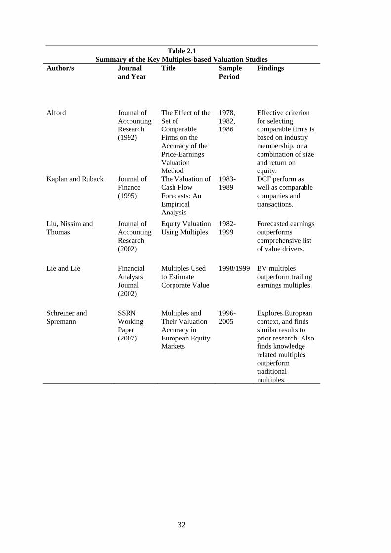
32

Table 2.1

Summary of the Key Multiples-based Valuation Studies

Author/s Journal

and Year

Title Sample

Period

Findings

Alford Journal of

Accounting

Research

(1992)

The Effect of the

Set of

Comparable

Firms on the

Accuracy of the

Price-Earnings

Valuation

Method

1978,

1982,

1986

Effective criterion

for selecting

comparable firms is

based on industry

membership, or a

combination of size

and return on

equity.

Kaplan and Ruback Journal of

Finance

(1995)

The Valuation of

Cash Flow

Forecasts: An

Empirical

Analysis

1983-

1989

DCF perform as

well as comparable

companies and

transactions.

Liu, Nissim and

Thomas

Journal of

Accounting

Research

(2002)

Equity Valuation

Using Multiples

1982-

1999

Forecasted earnings

outperforms

comprehensive list

of value drivers.

Lie and Lie Financial

Analysts

Journal

(2002)

Multiples Used

to Estimate

Corporate Value

1998/1999 BV multiples

outperform trailing

earnings multiples.

Schreiner and

Spremann

SSRN

Working

Paper

(2007)

Multiples and

Their Valuation

Accuracy in

European Equity

Markets

1996-

2005

Explores European

context, and finds

similar results to

prior research. Also

finds knowledge

related multiples

outperform

traditional

multiples.

33

CHAPTER 3 HYPOTHESES DEVELOPMENT

3.1 Introduction

The previous chapter outlined the prior research for multiples in general and

identified the gaps in the literature that provide the rationale for the thesis’ research

questions. This chapter develops hypotheses to address the research questions

relating to the valuation accuracy of multiples for companies involved in mergers

and acquisitions, and the subsequent effect on the price-to-intrinsic value ratio (P/V)

(the misvaluation proxy).

3.2 Valuation Accuracy of Multiples (RQ1 & 2)

The appealing characteristics of multiples may possibly explain their general use in

practice. First, an investor is able to efficiently gain an understanding of the relative

value between a set of equity securities when multiples are used. The calculations of

these multiples are generally simple and require widely available information such as

current share price, and historical (trailing) multiples or forecasted (forward)

multiples based on company financial data. Second, due to the simplicity and

widespread use of multiples, they are widely understood by market participants

(McCusker & Chang, 2007). Third, valuations based on multiples do not incorporate

arbitrary steady state assumptions which are involved in calculating terminal values,

which Sawyer and Joo (2004) state can account for more than 50 percent of the total

firm valuation.

However, multiples are not without their weaknesses. In the merger and acquisition

context, if a target is totally unrelated to the rest of the industry in terms of its risk,

size and growth potential, valuing a company based on multiples would lead to

spurious calculations of value. In addition, generally if the whole industry is

over/under valued, this will be reflected in the valuation of the target firm.

Furthermore in the case of loss-making firms, multiples are meaningless when using

historical earnings, as they result in negative valuations.

34

Schreiner (2007) note that different valuation methods imply competition, in which

only efficient methods of valuation will subsist into the future. Efficiency within the

context of valuation can be determined by the benefits of a valuation method

exceeding the costs of such a measure, with its cost benefit trade-off being required

to compare favourably against alternative methods of valuation, such as the

discounted cash flow model (Penman, 2004). Due to the simplistic nature of

calculating multiples, it can be classed as a “cheap” method of valuation. However,

in order to compete with more complex and theoretically sound valuation methods,

such as discounted cash flows and the residual income model, it requires a certain

level of valuation accuracy. Hence, the first research question is:

RQ1: How accurate are various multiple-based valuation methods in valuing

listed target and acquirer firms in Australia?

When calculating multiples for target and acquirers, independent experts and

investment advisers are faced with the decision to determine which appropriate value

driver to use. Thus, the next research question relates to the relative valuation

accuracy among the various multiples:

RQ2: Which of the various multiple-based valuation methods are more

accurate in valuing target and acquirer firms involved in takeovers in

Australia?

The discussion below will be used in formulating hypotheses about the general

ranking of value driver accuracy (to address RQ2). A caution concerning the prior

studies should be noted beforehand. The general ranking of the valuation accuracy of

value drivers in multiples in previous studies may or may not be observed in this

current study, due to different settings being involved (the takeover transaction) and

institutional differences. Previous studies have examined the valuation accuracy of

various value drivers for equity and entity multiple in general, rather than specifically

for takeover firms.

Several studies (including Kim & Ritter, 1999; Lie & Lie, 2002; Liu, Nissim, &

Thomas, 2002; Schreiner & Spremann, 2007) have documented the value-relevant

information contained in forward earnings as opposed to historical data. Liu et al.

(2002) suggest this forecasted earnings should be used as long as they are available.

35

This value relevance of information contained in forecasted earnings generally

results (as per previous studies) in low valuation errors. Thus, it is hypothesised that:

H1a: Value drivers based on forecasted earnings have lower valuation errors

than those based on historical value drivers.

In terms of valuation accuracy ranking of various historical value drivers, it is

anticipated that those income statement items closer to bottom line earnings will

perform better than those further up the income statement (for example Sales). This

is due to sales, gross income and EBIT(DA) by their very nature excluding valuable

information from the income statement (expenses), thus not fully reflecting

profitability (Schreiner & Spremann, 2007). Both Liu et al. (2002), Herrmann and

Richter (2003), and Schreiner and Spremann (2007) generally find this to be the case

for both equity and entity multiples (the latter based on the value of debt and equity).

Previous studies find extreme underperformance of multiples based on Sales which

exceeds multiples based on net cash flow from operations (NCFO), book value (BV)

and other earnings measures (Liu et al., 2002; Schreiner & Spremann, 2007). Though

a general ranking of historical value drivers has been observed in previous studies,

the issue of the most accurate value driver is still a subject of debate. Schreiner and

Spremann (2007) find earnings before tax (EBT) had a higher valuation accuracy

than bottom line earnings due to differences in tax rates across European countries.

This is not expected to be an issue in Australia, due to a national corporate tax rate of

30 percent levied on Australian resident companies. It is also interesting to note that

both Lie and Lie (2002) and Baker and Ruback (1999) find EBITDA has higher

valuation accuracy than EBIT, in contrast to other studies. From a theoretical point of

view, a vital weakness with using EBITDA in multiples is that it ignores the real

costs of taxation and capital expenditure that affect value (Suozzo, Cooper,

Sutherland, & Deng, 2001). Thus, prior literature is still inconclusive regarding the

best historical value driver. Therefore based on the above discussion, this study’s

next hypothesis is:

H1b: Value drivers closer to bottom line earnings (Net Income) have lower

valuation errors than those closer to the Trading Revenue income statement

line item.

36

Theoretically, in comparing earnings to cash flow as a value driver, it is argued that

earnings should be the more representative value driver because earnings reflect

value changes regardless of when the cash flow occurs. This includes the situation

regarding obligations to pay future employee entitlements (such as long service

leave), recognised as a current expense; however, a company’s cash flow remains

unchanged until such entitlements are paid. Another example involves purchase of

inventory for cash, which affects cash flow in the period purchased. However, this

transaction is only recognised as an expense, and affects value, when the inventory is

sold. Thus, earnings incorporate future cash flows that are value-relevant, whilst also

ignoring current-period cash flows that are not relevant to value (Liu et al., 2007).

However, earnings are not without their limitations. Many practitioners argue

accruals involve discretion, and may be used to manipulate earnings. Accounting

method choice can also impact on earnings. For example, the depreciation of assets is

often claimed to be accounted for on an ad hoc basis (Liu et al., 2002), rather than

truly reflecting the actual decline in value of non-current assets and the assets

replacement value. This study’s last hypothesis regarding valuation accuracy of

multiples is thus:

H1c: Value Drivers based on Earnings (excluding Trading Revenue) have

lower valuation errors than those based on net cash flow from operations

(NCFO).

3.3 Misvaluation of Takeover Firms Using Various Multiples to Estimate

Market Capitalisation (P) in P/V Ratios (RQ3)

As discussed in Chapter 2, many reasons have been given for the long-run

underperformance of acquirers, including: performance extrapolation (including

managerial hubris), method of payment, market fixation of EPS, and measurement

and research design issues, or a combination of any or all of these reasons. As

accounting-based multiples are commonly employed in corporate valuations in the

takeover context (for both the acquirer and the target), it raises the question as to

which of these multiples are more likely to lead to overpayment and thus long-run

underperformance of the acquirer. Thus, the third research question is:

37

RQ3: Which of the various multiple-based valuation methods is associated

with greater misvaluation (as measured by higher estimations of Price-to-

Intrinsic Value)?

Mathematically it can be shown that certain estimates of market capitalisation

derived from multiples will lead to particular results for valuation errors (scaled by

market capitalisation) as well as price-to-value (P/V) ratios, the latter being a

measure of over/under valuation. Four scenarios will be investigated: first, the

investigation of where estimated market capitalisation closely resembles the firm’s

actual market capitalisation; second, those instances where estimations of market

capitalisation are quite large and exceed actual market capitalisation; third, those

circumstances where estimation of market capitalisation are close to zero; and fourth,

further insights when Intrinsic Value is the value driver.

The formula below, taken from Liu et al. (2002), is used for calculating valuation

errors5 (εi/pit):

ti

ticti

ti

i

p

xp

p .

,.

.

(3.1)

First, estimations of market capitalisation that very closely resemble actual market

capitalisation, will result in low valuation errors (or valuation errors of zero), and

P/V calculations that closely resemble the P/V ratio when using actual market

capitalisation. Taking an ideal case of the estimated market capitalisation (tic x ,

)

equalling actual market capitalisation (pit), the latter can be substituted for the former

into the formula for calculating valuation errors (Equation 3.1).

ti

titi

ti

i

p

pp

p .

..

.

(3.2)

0.

ti

i

p

(3.3)

Using the example in Chapter 1, if the median multiple for the 10 Australian listed

companies was 11.39 instead of 20.99 (that is, WMC Resources ratio of market

capitalisation to Net Profit before abnormal items was approximately the same for

5 For more information on how this is derived, see section 4.3.1 in this thesis.

38

the rest of the firms in the industry), when valuing WMC Resources using multiples,

the estimated market capitalisation would be $8,380,842,699. The valuation error

would be as below:

ti

titi

ti

i

p

pp

p .

..

.

(3.2)

,699$8,380,842

,699$8,380,842-,699$8,380,842

.

ti

i

p

(3.4)

0.

ti

i

p

(3.5)

Thus, on average it could be said that the comparable multiple using this value driver

is effective in estimating the value of target firm.

Similarly, if the above substitution is also performed for estimating P/V ratios for

various value drivers, the P/V ratio for that value driver will closely resemble the

actual P/V ratio that uses market capitalisation. Thus, if actual P/V using market

capitalisation suggests over/under misvaluation, using multiples that have very close

estimations of market capitalisation (low valuation errors) will also reflect the same

over/under misvaluation. Using the numbers from the WMC Resources example:

ti

ti

ti

tic

V

p

V

x

.

,

.

,

(3.6)

,000$5,109,100

,699$8,380,842

,000$5,109,100

,699$8,380,842 (3.7)

64.164.1 (3.8)

Thus, both the actual P/V and the estimated P/V (using multiples) for this example

display possible overvaluation of the firm compared to WMC Resources Intrinsic

Value.

Second, estimations of market capitalisation that are quite large and exceed actual

market capitalisation, will result in large negative valuation errors, and high

estimations of P/V ratios. In the example below, the estimation of market

capitalisation ( tic x ,

) is assumed to be three times actual market capitalisation.

39

ti

titi

ti

i

p

pp

p .

..

.

3

(3.9)

ti

ti

ti

i

p

p

p .

.

.

2

(3.10)

2.

ti

i

p

(3.11)

Continuing the example of WMC Resources, if investment bankers used the median

multiple of the 10 comparable firms as per Chapter 1, the following valuation error

would be observed:

ti

ticti

ti

i

p

xp

p .

,.

.

(3.1)

,699$8,380,842

00)$736,000,0 x (20.99-,699$8,380,842

.

ti

i

p

(3.12)

84.0.

ti

i

p

(3.13)

The larger estimation of valuation relative to actual market capitalisation, the more

negative the valuation error. Algebraically, substituting estimated market

capitalisation for a value α times actual market capitalisation, (where α is a positive

value greater than one), the following outcome would result:

ti

titi

ti

i

p

pp

p .

..

.

. (3.14)

ti

ti

ti

i

p

p

p .

.

.

)1( (3.15)

)1(.

ti

i

p (3.16)

where (1-α) is negative due to the restriction α is positive and greater than one.

In contrast, these large positive estimations of market capitalisation will result in

higher P/V ratios, relative to smaller estimations of market capitalisation, holding the

Intrinsic Value constant (V), due to the large size of the numerator of P/V ratios. It

should be noted that when calculating valuation errors or P/V for a target or acquirer

for a particular takeover transaction, the denominator (market capitalisation or

40

Intrinsic Value) is held constant for each of the multiples, thus reflecting the

influence of the estimation of market capitalisation by each of the different multiples.

Therefore these calculations are more likely to result in a P/V suggesting

overvaluation (holding all other things constant) as indicated in the continuation of

the WMC Resources example below.

ti

i

ti

tic

V

P

V

x

..

,

(3.17)

02.3,000$5,109,100

00)$736,000,0 x (20.99 (3.18)

Thus, the larger the estimated market capitalisation relative to the actual market

capitalisation, the higher the possible misvaluation (contrast the Actual P/V for

WMC Resources (1.64), with a possibly greater overvaluation of 3.02 above).

Third, estimations of market capitalisation close to zero result in valuation errors

close to the value one (1), as well as low P/V calculations, holding Intrinsic Value

constant (V).

In the extreme case of estimated market capitalisation equalling to zero, substituting

into the valuation error formula, the following would be observed.

ti

ti

ti

i

p

p

p .

.

.

0

(3.19)

ti

ti

ti

i

p

p

p .

.

.

(3.20)

1.

ti

i

p

(3.21)

Thus, with WMC Resources, if the comparable median multiple was 2, the following

valuation error would be observed:

,699$8,380,842

00)$736,000,02(,699$8,380,842

.

x

p ti

i

(3.22)

82.0.

ti

i

p

(3.23)

41

Opposite to the last scenario considered for P/V calculations, the smaller the

estimation of market capitalisation, the smaller the P/V ratio (closer to

undervaluation than overvaluation).

ti

i

ti

tic

V

P

V

x

..

,

(3.24)

29.0,000$5,109,100

00)$736,000,02(

x (3.25)

The above P/V of 0.29 is far lower than both the two prior examples of 1.64 and 3.02

respectively.

Fourth, and lastly, regardless of valuation accuracy for the Intrinsic Value multiple,

the P/V calculation will demonstrate the misvaluation inherent in the comparable

median multiple (ie where xi,t = Vi,t).

ti

tic

ti

i

V

x

V

P

.

,

.

(3.26)

ti

tic

ti

i

V

V

V

P

.

,

.

(3.27)

c

ti

i

V

P

.

(3.28)

)(. c

c

ti

i

V

pmedian

V

P (3.29)

In hypothesising the performance of the P/V ratios based on various different

multiples, the conclusions below are drawn from mathematical logic. Multiples with

low valuation errors will also result in P/V ratios resembling those when actual

market capitalisation is used, and thus reflecting the over/undervaluation of the ratio

of actual market capitalisation to Intrinsic Value (P/V). Multiples with large negative

valuations errors will also result in high positive P/V ratios (suggesting possible

overvaluation). Lastly, multiples with valuation errors close to the value one (1) will

also result in low P/V ratios (suggesting possible undervaluation, or minimal

overvaluation), holding all other things constant. One last note: though the above

42

holds mathematically for each estimate individually, it does not automatically follow

that the mean or median value exhibited in valuation errors will also be the mean or

median value for P/V estimations. The above deductions do however give a guide to

the likely rankings of P/V estimations.

Liu et al. (2002), Lie and Lie (2002), Kim and Ritter (1999) and Schreiner and

Spremann (2007) all document low valuation errors for multiples using forecasted

earnings in general settings involving large samples. They do not specifically

investigate takeover firms. Different models are used amongst these studies for the

calculation of valuation errors, with low valuation errors in any of these models still

suggesting the same conclusions. That is, valuation error models that either calculate

a raw or absolute valuation error scaled by market capitalisations will still suggest

that estimated value (market capitalisation) is close to that of actual value (market

capitalisation). Thus, if the P/V ratios using actual market capitalisation suggest

overvaluation or undervaluation so will those estimations based on multiples with

low valuation errors.

For takeover transactions, it has also been observed that both acquirers and targets

are usually overvalued (based on the misvaluation proxy of the ratio of actual market

capitalisation to Intrinsic Value), with acquirers generally being more overvalued

than targets. Specifically, both Dong, Hirshleifer, Richardson, and Teoh (2006) and

Brown, Dong and Gallery (2005) document acquirers being more overvalued relative

to their targets, especially among takeovers that have shares as the form of

consideration and in merger bids, consistent with the model described by Shleifer

and Vishny (2003).

Thus, based on the prior literature, it is hypothesised that:

H2a: Estimations of P/V ratios using Forecasted Earnings Multiples are

close to P/V ratios based on actual market capitalisation.

Liu et al. (2002) find the most negative mean valuation errors using the median of

comparable firms from the same industry for multiples based on Cash Flow from

operations, Sales, BV and EBITDA. Schreiner and Spremann (2007) also find these

43

multiples produce high absolute valuation errors. However as they do not disclose

the result before taking absolute errors, it is difficult to determine whether the poor

performance is a result of a very high or very low estimation of market capitalisation.

Assuming that Schreiner and Spremann’s (2007) findings reflect those of Liu et al.

(2002) it is hypothesised that:

H2b: Estimations of P/V ratios based on bottom line earnings (net income)

are lower than those based on Trading Revenue, NCFO, BV and EBITDA

multiples.

Finally Liu et al. (2002) find that the multiple with Intrinsic Value as the value driver

results have the highest positive median valuation error. Thus, it is hypothesised that

multiples based on Intrinsic Value will also result in low estimations of the P/V ratio.

H2c: Estimations of P/V ratios based on Intrinsic Value multiples are lower

than those based on earnings or cash flow-based multiples.

Note also, as mentioned above, this estimation of P/V ratio based on Intrinsic Value

will reflect the median misvaluation of the industry comparables.

3.4 Conclusion

In this chapter hypotheses were developed based on prior literature to address the

research questions. In terms of valuation accuracy, these hypotheses predict that

value drivers based on forecasted earnings will have lower valuation errors than

those based on historical value drivers (H1a); that value drivers closer to bottom line

earnings (Net income) have lower valuation errors than those closer to the Trading

Revenue income statement line (H1b); and that value drivers based on earnings

(excluding Trading Revenue) have lower valuation errors than those based on net

cash flow from operations (NCFO) (H1c). In terms of misvaluation, these hypotheses

predict that estimations of P/V ratios using forecasted earnings multiples are closer to

P/V ratios based on actual market capitalisation (H2a); that estimations of P/V ratios

based on bottom line earnings (net income) are lower than those based on Trading

Revenue, NCFO, BV and EBITDA multiples (H2b); and that Estimations of P/V

ratios based on Intrinsic Value multiples are lower than those based on earnings or

44

cash flow based multiples. The next chapter presents the research design that will be

used to test the hypotheses.

45

CHAPTER 4 RESEARCH DESIGN

4.1 Introduction

This chapter describes the research design used to test the research hypotheses

developed in the previous chapter. Initially, the sampling procedure and data sources

will be described. The research design that follows will be split into two main

sections. The first will describe the methods used to test the valuation accuracy of

multiples (research questions 1-2 and hypotheses H1a-c), based on valuation

analysis. The second will describe the methodology employed to estimate

misvaluation of firms based on using multiples to estimate a price to Intrinsic Value

(P/V) measure (research question 3 and hypotheses H2a-c). Lastly, the potential

limitations of the research design will be discussed.

4.2 Sampling Procedure and Data Sources

The sample used in this study consists of takeover transactions completed between 1

January 1990 and 31 December 2005. The observations are primarily drawn from the

Connect 4 database. Financial statement data is obtained from the Morningstar

FinAnalysis database. Industry classifications were obtained from the Share Price

and Price Relative (SPPR) database maintained by the Australian Business School.

Missing market capitalisations from FinAnalysis have also been sourced from the

SPPR. Analyst forecasts of future earnings are sourced from the Thomson Reuters’

I/B/E/S database. Sensitivity analysis in Chapter 6 includes the actual market

capitalisation one, two and three years after the takeover announcement date, thus

using market capitalisation up to 2008.

The following criteria are used in the sample selection process for takeovers: (1) both

the target and the acquirer must be Australian firms; (2) the acquirer must be listed

on the ASX, or be a subsidiary of a listed company; and (3) the target must be listed

on the ASX. A full summary of the sample selection procedures is presented in Table

4.1. The requirement that the target and acquirer be Australian is to ensure the

46

availability and comparability of necessary data. Fuller, Netter and Stegemoller

(2002) find that the returns to the acquiring firm depend on the organisational form

of the acquired asset, that is, whether the target is a private firm, public firm or

subsidiary. Thus, to ensure homogeneity of the sample and availability of data, it is

required that all targets must be listed.

As a subsidiary taking over a firm is in essence the same as if the parent performed

the takeover, this study includes firms where the acquirer is a listed firm or a

subsidiary of a listed firm. However, similar to Brown, Dong and Gallery (2005), this

study does not investigate targets that are subsidiaries of unlisted firms due to the

identification difficulties. These target firms are possibly subject to discretionary use

of accounting information by the parent company in order for them to achieve a

higher sale price for the target.

Following on from Frankel and Lee (1998) and Brown et al. (2005) for calculations

of P/V, firms with negative book value (BV) are also dropped from the sample. This

is due to the inability of interpreting return-on-equity (ROE) for these firms in

economic terms (Frankel & Lee, 1998).

Similar to Liu, Nissim and Thomas (2002), and Schreiner and Spremann (2007), for

the main part of this study, it is required that both the acquirer and its corresponding

target have positive values for each of the value drivers examined (the value drivers

required will be listed in the next section). This allows comparison amongst value

drivers. For historical values, these value drivers will be derived from data obtained

from the most recently issued financial statements within the last 18 months prior to

the takeover to allow for firms who change reporting dates. Similar to Dong,

Hirshleifer, Richardson, and Teoh (2006) and Brown et al. (2005), it is also required

that there is at least 30 days before the announcement of the takeover takes place to

ensure that the information is available to the public at the time of the announcement.

I/B/E/S forecasts used are those at least 30 days before the announcement of the

takeover takes place, a practice also followed by Brown et al. (2005). To ensure the

analyst forecasts are not subject to staleness, each I/B/E/S forecast used is the median

or mean of at least three different analysts.

47

Table 4.1

Sample Size Selection

Acquirer Target

Takeovers 867 867

Less Missing Financial Information -406 -222

461 645

Less Missing Analyst Forecasts -236 -424

225 221

Less Negative Value Drivers -54 -71

171 150

Less Insufficient Comparable Firms -24 -21

Sample Size 147 129

Details regarding the calculation of the Intrinsic Value (based on the Residual

Income Model) are detailed below, as well as in Appendix A. It should be noted that

similar to I/B/E/S forecasts, the Intrinsic Value is calculated at least 30 days before

the announcement takes place. Requiring at least 30 days before the announcement

for both the I/B/E/S forecasts and Intrinsic Value reduces any possible pre-run up of

share price that the firm may have encountered, which thus could affect valuations.

Liu et al. (2002) and Schreiner and Spremann (2007) require that all comparable

firms have positive values for all value drivers. This study however does not require

comparables to meet this stringent requirement, for two reasons. First, this

effectively biases the comparable firms to only include profitable firms, as firms with

negative values for any driver (for example net profit after tax (NPAT) after

abnormals or NCFO) would be excluded from their study. Second, it is unlikely that

an investment banker, or those involved in valuing a company using multiples would

simply exclude a firm on the basis of one value driver being negative, unless the

value driver is the specific one used for their valuation. Liu et al. (2002) document

when this requirement is relaxed so that each comparable must have a positive value

for only Sales and forecasted Earnings, that the relative performances of value

drivers are still observed. However, the dispersion of valuation error increases for

each firm. Thus, the valuation errors for this study are likely to be larger than

encountered in a positive value restriction context.

48

4.3 Valuation Accuracy of Multiples

In this section the model used to test the valuation accuracy of multiples will be

described to address RQ1. This will be followed by the identification of value

drivers, followed by the description of the basis of selecting comparable firms. These

components will provide the basis for addressing RQ2 and testing the related

hypotheses (1a-c) with respect to which of the various multiple-based valuation

methods are more accurate in valuing target and acquirer firms involved in takeovers

in Australia.

4.3.1 Valuation Accuracy Model

The first stage of analysis involves an investigation of the accuracy of various

multiples to estimate a firm’s market capitalisation compared to the stock market

capitalisation 30 days prior to the takeover announcement. Multiples are the ratio of

a firm’s market capitalisation to a particular value driver6. The estimation of a firm’s

market capitalisation is the firm’s value driver (for example EBITDA), multiplied by

the median multiple of a firm from the same industry. Valuation analysis involves

examining the difference between actual market capitalisation and the estimated

market capitalisation based on multiples. Alford (1992) commented that the benefits

of valuation analysis compared to regression analysis include that valuation analysis

does not assume a linear model for multiples, as well as valuation analysis makes

fewer distributional assumptions.

In the first stage of the analysis, the traditional ratio representation is followed, by

requiring that the estimated market capitalisation of a firm (p (pi,t)) is directly

proportional to the value driver xi of the firm in the period before the transaction:

pi,t = βc xi,t-1 + εi,t (4.1)

where βc is the multiple of the value driver, and εi,t is the valuation error. To improve

efficiency, equation (4.1) is divided by the transaction value:

6 Value drivers are explained in more detail below.

49

ti

i

ti

ti

cpp

x

..

1,1

(4.2)

The valuation error (εi,t) in equation (4.1) is unlikely to be independent of firm value,

as larger values of firm value are likely to have higher absolute valuation errors

(Schreiner, 2007). Baker and Ruback (1999) and Beatty, Riffe and Thompson (1999)

find the valuation error (residual (εi)) is proportional to value. Thus, it is expected

that estimations of the slope in equation (4.2) will provide more accurate estimates of

the slope than equation (4.1) when using market capitalisation.

Unlike Liu et al. (2002) and Schreiner and Spremann (2007), for estimation of the

multiple ( c ), the restriction that expected scaled valuation errors E[εi/pi,t] is zero is

not imposed7. By rearranging equation (4.2), the multiple c can be estimated using

the harmonic mean or median as an appropriate measure of central tendency. The

estimate of c is multiplied by the target firm’s value driver to obtain an estimation

for the target firm equity value. As such, similar to Liu et al. (2002), the pricing

errors are calculated as follows:

ti

ticti

ti

i

p

xp

p .

,.

.

(4.3)

To evaluate the performance of various multiples, measures of dispersion for the

pooled distribution of scaled valuation errors εi/pi,t (hereafter valuation errors) will be

examined. The key performance measures are the median (both raw and in absolute

terms) valuation errors; the dispersion of valuation errors (as measured by the

standard deviation and inter-quartile range); as well as the fraction of absolute

valuation errors below 15 percent of market values (transaction values). These

measures will then allow comparability with previous studies, including Liu et al.

(2002), Schreiner and Spremann (2007), Kaplan and Ruback (1995), Kim and Ritter

(1999), and Lie and Lie (2002).

7 It was noted in Liu et al. (2002), that when unbiased expected valuation errors were applied, relative

rankings were left unadjusted. Sensitivity analysis in this study showed by restricting the study to

unbiased valuation errors (where lower weights are in effect assigned to extreme valuation errors

relative to unrestricted expected valuation errors), valuation errors and relative rankings were

significantly affected. This may also be due in part to the study not applying the restriction of

comparable firms requiring positive values for each value driver, thus also leading to higher valuation

errors.

50

To reduce the effect of outliers, Liu et al. (2002) trim the top and bottom one percent

of the valuation errors for each of the value drivers. However, due to the relatively

small dataset used in this thesis, avoidance of data loss is desirable. Thus, this study

employs winsorising, at the 2.5 percent and 97.5 percent levels in the tails of the

distributions.

4.3.2 Value Drivers

The value drivers used are: Trading Revenue (or sales), EBITDA (earnings before

interest, tax, depreciation and amortisation), EBIT (earnings before interest and tax),

earnings before abnormal items, bottom line earnings, net cash flow from operations

(NCFO), book value (BV), analyst forecasts of EPS for one year (FEPS1) and two

years ahead (FEPS2) and Intrinsic Value based on the residual income model

(Intrinsic Value).

These drivers were chosen for two reasons. First, the majority of these value drivers

have been investigated in prior multiples valuation accuracy literature, (Lie and Lie,

2002; Liu et al., 2002; Schreiner and Spremann, 2007). Second, based an analysis of

valuation method in a sample of Australian takeovers documents (in independent

expert reports) from 1996 to 2005, of those reporting the use of multiples as their

primary valuation method, 51.6 percent used EBITDA, followed by bottom line

earnings (18.3 percent), EBIT (17 percent), with the remaining using measures of

EBITA (EBIT before amortisation) and EBITD (EBIT before depreciation). (The

relevant Morningstar FinAnalysis items are included in Appendix B.)

4.3.3 Comparable Firms

For each target/acquirer, a minimum of five comparable firms are selected based on

industry membership. Alford (1992) comments that comparable firms in the same

industry are generally selected due to their assumed similar risks and earnings. They

also often use similar accounting methods. In their study, Bhojraj, Lee and Oler

(2003) find that GICS classifications are significantly better than the Standard

Industrial Classification (SIC) codes, North American Industry Classification System

(NAICS) codes and the Fama and French (1997) industry grouping at explaining

51

stock returns co-movements and cross sectional variations in valuation multiples.

The SPPR database records the industry classification for the listed Australian

companies. Two issues arise in industry classification of firms. First, by selecting

industry membership based on the most current industry grouping, firms that have

changed industry are misclassified for the period of time in the previous industry.

Second, GICS was introduced in Australia in September 2002, with classification

information available in July 2001. Thus, firms that delisted before July 2001 are

without GICS classification (a potential problem, especially as target firms are a

major component of delisted firms), thus creating survivorship bias. To overcome

these issues, monthly industry classifications are sourced from SPPR. Industry

classifications before July 2001 are based on the previous ASX Industry

Classification, with industry classifications from July 2001 based on the more recent

GICS classification.

4.4 Estimation Procedure for Misvaluation Proxy (P/V)

In this section, the procedure for testing which of the various multiple-based

valuation methods is associated with greater misvaluation (as measured by higher

estimations of Price-to-Intrinsic Value) are described. Both Dong et al. (2006) and

Brown et al. (2005) define misvaluation as the difference between current market

price and a measure of non-market-based fundamental value. It also reflects the

discrepancy between the investors’ predictions concerning the future earnings

potential of the firm, and the firm’s share price (Dong, 2003). Both of these studies

use the residual income model (RIM) as a measure of fundamental value, with the

ratio of residual income value to price (P/V or its inverse V/P) as the proxy for

market misvaluation. As this study examines the effect of multiple valuation method

on misvaluation, estimated market capitalisation is calculated using comparable

multiples rather than a firm’s current market capitalisation.

As previously indicated, to eliminate the run-up effect that is often observed prior to

major corporate events, the estimated price used in P/V calculations are computed,

wherever possible, using comparable firms market capitalisation 30 days before the

takeover announcement (Brown et al., 2005; Dong et al., 2006). Dong et al. (2006)

52

also remark that this ensures information required for calculating V/P is available

before the takeover announcement.

Several studies document strong support for P/V as a superior measure of

misvaluation to various other measures including price to book value (P/B) ratio (Ali,

Hwang, & Trombley, 2003; Frankel & Lee, 1998; Lee, Myers, & Swaminathan,

1999). Dong et al. (2006) ascribe the superiority of P/V to its insensitivity to various

accounting treatments and its ability to capture forward looking information that is

reflected in analysts’ earnings forecasts. Dong et al. (2006) however also note that

the P/V measure is affected by analysts’ forecasts biases that are correlated with

widespread market misvaluation. Despite this weakness, they find that for their

sample of U.S. takeover firms, P/V has significant explanatory power above P/B.

The Intrinsic Value (V) is calculated using the residual income model, and has also

been referred to as the Edwards-Bell-Ohlson (EBO) valuation equation, the latter

being coined by Bernard (1994). Recent uses of this model are most often based on

the theoretical work by Ohlson (1990, 1995), Lehman (1993) and Feltham and

Ohlson (1995). Earlier related work on the residual income value dates back as early

as the 1930s, including the work of Preinreich (1938), Edwards and Bell (1961) and

Peasnell (1982). Several approaches to empirically implement the residual income

model include Penman and Sougiannis (1998), Dechow, Hutton and Sloan (1999),

Frankel and Lee (1998), and more recently in takeover contexts (Brown et al., 2005;

Dong et al., 2006), and in seasonal equity offerings (Brown, Gallery, & Goei, 2006).

The residual income model uses a foundation of clean surplus accounting, that is,

where all gains and losses that affect BV are included in earnings. Put differently,

BV in period t+1 can be found by first adding earnings in period t+1 to BV in period

t, then subtracting net dividends in period t+1 (Brown et al., 2005):

BVt+1 = BVt + NIt+1 – Dt+1 (4.4)

where: BVt+1 = Book value in period t+1

NIt+1 = Net income (earnings) in period t+1

Dt+1 = Dividend paid in period t+1

53

Lee et al. (1999) and Ali et al. (2003) find that the number of periods in the expanded

term residual income models is immaterial once it exceeds three periods and has the

most predictive power in the analysis of Lee et al.’s (1999) study. Further

descriptions of the calculation of the Intrinsic Value (V) are included in Appendix A.

Similar to Dong et al. (2006), P/V ratios are winsorised to remove the influence of

outliers. As previously explained in this thesis, P/V ratios are winsorised at 2.5

percent and 97.5 percent in the tails of distributions.

4.5 Limitation of the Research Design

To enable comparison across a range of multiples, it has been necessary to restrict

the target and acquirer companies evaluated to those with positive values for each of

the value drivers. This unavoidably biases the sample, and hence application of

results to profitable targets and acquirers. However, it is also understandable that

firms with poor performance in the past (negative value drivers) are unlikely to be

valued based on multiples, to avoid negative valuations. In order to ensure available

data, a further restriction is that the targets and acquirers be listed companies, thus

possibly creating results that may or may not be generalisable to unlisted firms.

As mentioned above, consistent with the studies of Dong et al. (2006) and Brown et

al. (2005) to mitigate any effect of the takeover on share price, the value of market

capitalisation used to calculate P/V ratios are taken at least 30 days before the

announcement of the takeover. However, as mentioned by Brown et al. (2005), this

creates an arbitrary cut-off, as different takeovers may experience varying share price

movements due to differences in the amount and timing of information leakages.

4.6 Conclusion

This chapter has described the sample, study period and data sources relevant to the

study. It then described the methodology that is employed to address the research

questions and to test the related hypotheses. This includes the use of valuation

analysis (RQs 1 and 2, hypotheses 1a-c) to find the valuation accuracy of certain

multiples, and the use of P/V ratios to test the overvaluation of these multiples (RQ3

54

and hypotheses 2a-c). The next two chapters report the results of the testing of the

procedures documented above.

55

CHAPTER 5 RESULTS

5.1 Introduction

In this chapter the testing of the hypotheses is conducted. First, the valuation

accuracy hypotheses are tested using the pricing error model described in Chapter 4,

with absolute median valuation error being used to rank the multiples in terms of

accuracy. Second, the misvaluation hypotheses are tested using the ratio of estimated

price (as calculated by the multiple) to Intrinsic Value (based on the residual income

model), with higher values of P/V representing overvaluation.

5.2 Descriptive Statistics

Consistently throughout the thesis and where applicable, Panel A and B will display

the results of acquirers and targets respectively. Table 5.1 presents the descriptive

statistics for the acquirer (147) and target (129) firms. Value drivers of both

acquirers and targets are negatively skewed, with means higher than medians. The

skewness implies that for both samples, there exists a proportion of firms which are

far larger in terms of value drivers than the rest of the sample. It can also be noted

that for each value driver, the mean, median, standard deviation and inter-quartile

range are higher for acquirers than for targets. Thus, in general, acquirers are larger

(in terms of value drivers) than targets.

5.3 Valuation Accuracy of Multiples Results

The following statistics that describe the distribution of the valuation errors are

reported: two measures of central tendency (mean and median) and three measures of

dispersion (the standard deviation, and two non-parametric measures: the inter-

quartile range; and the distribution of the middle 80 percent of the data, as calculated

as the 10th

percentile subtracted from the 90th

percentile). Similar to Schreiner and

Spremann (2007), the fraction of valuation errors within 15 percent of zero (zero

representing no valuation error), and then within 25 percent of zero, are also

included. Results are separated into three categories: historical, forecasted and

Intrinsic Value drivers. Of the historical value drivers book value (BV), net cash flow

56

from operations (NCFO), and trading revenue are generally explored separately, with

the remaining falling under the title historical earnings value drivers.

Similar to Schreiner and Spremann (2007), ranking in the following section will be

based mainly on absolute valuation error, specifically median absolute valuation

error. The examination of valuation errors in signed form (that is, before absolute

values) is presented as part of the analysis of price to Intrinsic Value (P/V) ratios.

5.3.1 Valuation Accuracy of Multiples Based Valuations in General (RQ1)

Research Question 1 asks how accurate are various multiple-based valuation

methods in valuing listed acquirers and targets in Australia. Similar to Schreiner

(2007) and given the non-normality evident, median absolute valuation errors will be

used as the basis of determining the accuracy of such methods.

The acquirer and target absolute valuation error results are listed in Table 5.2, Panel

A and B. In general, signed valuation errors are negatively skewed (with medians

greater than means), with absolute valuation error being positively skewed. For both

targets and acquirers, all multiples (except the multiples based on BV and trading

revenue) have median absolute valuation errors lower than 30 percent. These results

are similar to Schreiner and Spremann (2007) for their European sample. Schreiner

and Spremann find six corresponding multiples with median absolute valuation

errors lower than 30 percent. Furthermore, this study finds seven acquirer and six

target multiples with median absolute valuation errors within 25 percent of a firm’s

market capitalisation. Median absolute valuation errors range from 16.0 percent to

42.9 percent for acquirers and 19.0 to 46.9 for targets. This is comparable with

Schreiner and Spremann’s (2007) range of 21.5 percent to 43.8 percent for 27

multiples for their European sample. Thus, in answer to RQ1, valuations based on

multiples generally produce estimates within 30 percent of actual market

capitalisation, which is comparable with prior literature in other contexts.

When comparing the results of acquirers to targets, acquirers have lower mean

absolute valuation errors for all multiples examined, coupled with lower standard

deviations for all bar FEPS2 and lower inter-quartile ranges for all bar EBITD and

57

NPAT before abnormals. Eight of the thirteen multiples also have lower median

absolute valuation errors than their target counterpart. This may in part be due to

acquirers having larger value drivers as mentioned above and consistent with Alford

(1992) who documented higher valuation accuracy amongst larger firms as compared

to smaller firms.

In undocumented results, when acquirers are restricted to multiple bidders (52% of

the sample), there is an improvement in the median absolute valuation errors range

(from 14.2 percent to 38.4 percent), with all bar the multiple based on Intrinsic Value

displaying lower median absolute valuation errors than the results in Table 5.2, Panel

A. Thus it appears than the more frequent participants in mergers and acquisitions

have greater valuation accuracy.

58

Table 5.1

Distribution of Value Drivers

Panel A: Acquirers

Value Driver N Mean Median Std Dev Skewness Kurtosis

1st

Quartile

3rd

Quartile

75%-

25%

90%-

10%

Historical Value

Drivers 6 2 3 7 8 9 10 11 12 13

Trading Revenue 147 1574.7 348.1 4550.2 5.4 30.1 129.2 1188.0 1058.8 3125.4

EBITDA 147 285.6 107.9 871.0 10.4 118.0 46.4 271.8 225.5 534.4

EBITD 147 273.0 97.0 863.9 10.5 119.5 42.8 251.5 208.8 489.3

EBITA 147 229.1 79.9 656.8 10.2 115.6 39.3 239.9 200.5 450.8

EBIT 147 216.2 73.5 649.5 10.3 117.6 31.7 222.8 191.1 421.5

EBT 147 190.2 69.2 596.8 10.5 119.5 29.2 187.5 158.3 357.7

NPAT before abnormals 147 140.0 47.6 427.0 10.4 118.7 18.9 124.7 105.7 267.1

NPAT after abnormals 147 139.5 47.7 435.4 10.2 115.3 17.0 123.5 106.5 274.6

NCFO 147 208.9 83.2 661.9 10.2 114.7 27.9 181.5 153.6 388.1

BV 147 1092.1 456.9 2157.9 7.0 65.4 188.1 1224.4 1036.3 2607.4

Intrinsic Value Driver

Intrinsic Value 147 1871.7 584.7 5180.5 8.8 91.1 251.7 1632.0 1380.3 3816.6

Forecast Value Driver

FEPS1 147 152.5 53.7 381.2 8.9 93.7 24.9 158.3 133.4 312.8

FEPS2 147 180.6 58.4 486.9 8.3 78.7 28.7 165.9 137.2 323.9

Other Measures

Market Capitalisation 147 2226.3 751.6 5300.0 8.5 87.2 364.2 2460.3 2096.0 4203.6

P/V 147 1.5559 1.2932 0.9125 3.4 21.7 1.0217 1.9420 0.9203 1.5743

59

Table 5.1 continued

Distribution of Value Drivers

Panel B: Targets

Value Driver N Mean Median Std Dev Skewness Kurtosis

1st

Quartile

3rd

Quartile

75%-

25%

90%-

10%

Historical Value

Drivers 6 2 3 7 8 9 10 11 12 13

Trading Revenue 129 711.3 264.2 1172.9 2.7 7.2 77.7 697.0 619.3 2175.6

EBITDA 129 149.8 61.4 243.1 3.4 12.8 33.5 143.9 110.4 311.1

EBITD 129 138.0 56.5 220.8 3.4 13.4 29.7 137.2 107.5 275.6

EBITA 129 119.8 49.4 196.0 3.9 18.3 28.9 130.9 102.0 241.4

EBIT 129 107.8 45.2 179.4 4.2 22.3 25.7 116.3 90.6 216.4

EBT 129 89.1 37.1 138.5 3.6 16.0 21.8 98.4 76.6 199.6

NPAT before abnormals 129 72.3 31.2 120.9 3.8 16.1 16.4 70.3 53.9 127.3

NPAT after abnormals 129 75.0 30.4 155.1 5.4 36.2 13.1 70.3 57.2 140.6

NCFO 129 116.1 45.8 207.4 4.1 19.9 22.7 106.8 84.0 235.0

BV 129 741.4 341.0 1264.7 3.4 11.7 122.1 672.5 550.4 1431.0

Intrinsic Value Driver

Intrinsic Value 129 1009.9 437.3 1693.5 3.7 15.6 198.8 1022.0 823.1 2177.8

Forecast Value Driver

FEPS1 129 93.6 34.3 197.6 4.6 22.8 17.4 79.2 61.8 143.2

FEPS2 129 103.7 39.8 251.7 7.3 66.0 19.8 81.0 61.2 191.9

Other Measures

Market Capitalisation 129 1176.9 464.5 2037.0 3.7 16.5 204.2 1280.4 1076.2 2582.7

P/V 129 1.2414 1.0911 0.7376 3.7 23.2 0.8610 1.4690 0.6080 1.1992

Notes

Amounts in $ millions.

FEPS is Forecast Earnings Per Share. The number following relates to the forecast period (FEPS1 is one year ahead Forecast Earnings Per

Share). FEPS based on median analysts’ forecasts are selected.

Other variables as described in Appendix C.

60

Table 5.2

Absolute Valuation Errors

Panel A: Acquirers

Multiples based on median of comparable firms from the same industry

Value Driver N Mean Median Std Dev Skewness Kurtosis

1st

Quartile

3rd

Quartile

75%-

25%

90%-

10%

Fraction

<.15

Fraction

<.25

Historical Value

Drivers 6 2 3 7 8 9 10 11 12 13 15 16

Trading Revenue 147 0.6272 0.4288 0.7519 2.5744 6.2230 0.2239 0.6722 0.4482 1.2566 0.1769 0.2789

EBITDA 147 0.3040 0.2163 0.2865 1.9944 4.8249 0.1098 0.4348 0.3250 0.5781 0.3605 0.5374

EBITD 147 0.3217 0.2504 0.3167 2.0570 5.1299 0.0961 0.4365 0.3404 0.6006 0.3605 0.4966

EBITA 147 0.2924 0.2187 0.2340 1.2467 1.2474 0.1160 0.3947 0.2787 0.5409 0.3197 0.5442

EBIT 147 0.3099 0.2186 0.2865 1.8252 3.5686 0.1138 0.3945 0.2807 0.5948 0.3197 0.5374

EBT 147 0.3062 0.2316 0.3097 2.1958 5.1274 0.0974 0.3844 0.2870 0.5318 0.3537 0.5510

NPAT before

abnormals 147 0.2875 0.2386 0.2272 0.8877 0.0957 0.0976 0.4374 0.3398 0.5320 0.3605 0.5170

NPAT after abnormals 147 0.3387 0.2832 0.2848 0.9984 0.3780 0.1013 0.4988 0.3975 0.6924 0.3333 0.4762

NCFO 147 0.3931 0.2840 0.3488 1.5533 2.9209 0.1306 0.5681 0.4375 0.7945 0.2925 0.4490

BV 147 0.3408 0.3043 0.2332 0.3812 -0.9258 0.1509 0.4993 0.3484 0.6411 0.2517 0.4082

Intrinsic Value Driver

Intrinsic Value 147 0.3040 0.2853 0.2221 0.5457 -0.5510 0.1198 0.4674 0.3475 0.5843 0.3129 0.4830

Forecast Value Driver

FEPS1 147 0.2734 0.1722 0.2965 2.4201 6.6229 0.0815 0.3583 0.2768 0.5094 0.4082 0.6463

FEPS2 147 0.2568 0.1597 0.3233 3.1400 10.8936 0.0767 0.3110 0.2343 0.4236 0.4490 0.6667

61

Table 5.2 continued

Absolute Valuation Errors Panel B: Targets

Multiples based on median of comparable firms from the same industry

Value Driver N Mean Median Std Dev Skewness Kurtosis

1st

Quartile

3rd

Quartile

75%-

25%

90%-

10%

Fraction

<.15

Fraction

<.25

Historical Value

Drivers 6 2 3 7 8 9 10 11 12 13 15 16

Trading Revenue 129 1.1902 0.4689 2.4433 3.7331 13.9160 0.1568 0.8350 0.6782 2.4399 0.2326 0.3566

EBITDA 129 0.4827 0.2299 0.7913 3.1619 9.7492 0.1059 0.4964 0.3904 0.9687 0.3953 0.5194

EBITD 129 0.4976 0.2379 0.8327 3.3126 10.9078 0.1063 0.4279 0.3215 0.9674 0.3721 0.5039

EBITA 129 0.3975 0.2500 0.4928 2.5976 7.0124 0.1026 0.4795 0.3770 0.7448 0.3566 0.4961

EBIT 129 0.4537 0.2393 0.6441 2.8438 7.9307 0.1329 0.4495 0.3166 0.9206 0.3178 0.5039

EBT 129 0.4442 0.2513 0.7272 3.5294 12.8439 0.0943 0.4206 0.3263 0.7546 0.3643 0.4961

NPAT before

abnormals 129 0.3358 0.2281 0.3712 2.5655 7.7458 0.1178 0.4120 0.2942 0.6511 0.3256 0.5581

NPAT after abnormals 129 0.3936 0.2634 0.3713 1.6137 2.5149 0.1332 0.5678 0.4347 0.7802 0.3101 0.4961

NCFO 129 0.4605 0.2796 0.5398 2.7787 8.9922 0.1483 0.6177 0.4694 0.7958 0.2636 0.4574

BV 129 0.6695 0.3131 1.1332 3.2015 10.0595 0.1412 0.5740 0.4328 1.3586 0.2713 0.4186

Intrinsic Value Driver

Intrinsic Value 129 0.8028 0.2593 2.0937 3.9064 14.0285 0.0890 0.4763 0.3874 0.7923 0.3721 0.4961

Forecast Value Driver

FEPS1 129 0.3810 0.1966 0.4647 2.4508 6.3934 0.1097 0.5057 0.3960 0.7329 0.3953 0.5814

FEPS2 129 0.2945 0.1900 0.3135 2.2484 5.5308 0.1090 0.3438 0.2348 0.6560 0.4031 0.6047

Notes

FEPS is Forecast Earnings Per Share. The number following relates to the forecast period (FEPS1 is one year ahead Forecast Earnings Per Share).

FEPS based on median analysts’ forecasts are selected.

Other variables as described in Appendix C.

Fraction <.15 and <.25 refers to the percentage (expressed as a decimal) of those valuation errors with an absolute value between 0 and 0.15,

and 0 and 0.25 respectively.

62

5.3.2 Valuation Accuracy of Various Multiples Based Valuations (RQ2)

Research question 2 (RQ2) asks which of the various multiple-based valuation

methods are more accurate in valuing acquirer and target firms involved in takeovers

in Australia.

In terms of relative performance (when using the median absolute valuation error),

the following general rankings are observed in Table 5.2, Panel A, for acquirers:

1) Multiples based on forecast earnings

2) Multiples based on historical earnings

3) Multiples based on NCFO, Intrinsic Value, and BV

4) Multiples based on Trading Revenue

In terms of relative performance (when using the median), the following general

rankings are observed in Table 5.2, Panel B, for targets:

1) Multiples based on forecast earnings

2) Multiples based on historical earnings and Intrinsic Value

3) Multiples based on NCFO and BV

4) Multiples based on Trading Revenue

Hypothesis Tests (H1a-c)

Hypothesis H1a predicts that forecasted value drivers have lower valuation errors

than historical value drivers. Table 5.2, Panel A, reveals that for acquirers, multiples

based on forecasted earnings have the lowest median and mean absolute valuation

errors for all the multiples examined in this study, as well as the smallest inter-

quartile range. Specifically, the median absolute valuation errors for these two

multiples are within 20 percent of actual market capitalisation (17.22 percent for

FEPS1, and 15.97 percent for FEPS2). Similarly, in Table 5.2, Panel B, for targets,

multiples based on forecasted earnings have the lowest median absolute valuation

errors of the multiples examined for both FEPS1 and FEPS2 (19.66 percent and

19.00 percent respectively), with multiples based on FEPS2 additionally having the

lowest mean and inter-quartile range. For both acquirers and targets the median,

mean and inter-quartile range all improve when the forecast horizon moves from one

year ahead (FEPS1) to two years ahead (FEPS2). As mentioned by Liu et al. (2002),

63

the superiority of forecasted earnings over historical value drivers is intuitively

appealing as the former should reflect future profitability better than the latter, with

accuracy improving as the forecast horizon increases. Thus, similar to prior research,

this thesis finds evidence that multiples based on forecasted value drivers have

higher valuation accuracy than multiples based on historical value drivers as

predicted (hypothesis H1a).

Hypothesis H1b predicts that value drivers closer to bottom line profit will have

lower valuation errors than those closer to the income statement line item trading

revenue. From Table 5.2, the median absolute valuation errors for multiples based on

historical earnings metrics range from 0.2163 (EBITDA) to 0.2832 (NPAT after

abnormals) for acquirers, and 0.2281 (NPAT before abnormals) and 0.2634 (NPAT

after abnormals) for targets. Contrary to expectations, for both acquirers and targets,

lower valuation errors are not entirely exhibited by value drivers closer to bottom

line profit than those closer to the income statement line item trading revenue. For

both samples, the EBITDA multiple (0.2163 for acquirers and 0.2299 for targets) has

a lower median absolute valuation error than NPAT after abnormals, as well as

NPAT before abnormals for acquirers. On the other hand, as mentioned above, the

NPAT before abnormals multiple for targets has the lowest median absolute

valuation errors of the historical measures examined.

Additionally, there are some trends evident for historical multiples. First, for

acquirers with the exception of the EBITDA multiple, there is a gradual

improvement from the income statement line item trading revenue to EBIT, with

EBT, NPAT before abnormals and NPAT after abnormals progressively showing

larger absolute median valuation errors. This tends to indicate that acquirer firms

have similar EBIT multiples to that of their industry, with differing value relevance

of interest, tax and abnormals reflected in either the firm’s or comparable firms’

market capitalisation. This pattern is also evident in the acquirers’ inter-quartile

range, though arching around the EBITA multiple instead.

Second, for both acquirers and targets the absolute median and mean valuation error,

standard deviation and inter-quartile range are highest for the multiple based on

Trading Revenue. Specifically, the multiple based on Trading Revenue for acquirers

64

and targets is the only multiple in the sample with absolute median valuation errors

over 40 percent (46.89 percent and 42.88 percent respectively). Thus, as mentioned

by Schreiner and Spremann (2007), multiples based on earnings include some degree

of pertinent information about profitability that is not contained in Trading Revenue.

Third, a lower absolute median valuation error is exhibited by the multiple derived

from NPAT before abnormals, as opposed to after abnormals. This may in part be

due to the transitory nature of abnormals, which differ from year to year and may or

may not be specific to a particular firm. As mentioned above, NPAT after abnormals

has highest median absolute valuation errors of the historical earnings multiples

examined. Comparing this to Schreiner and Spremann’s (2007) U.S. and European

sample, bottom line earnings in an Australian takeover context more closely

represents that of the European sample (where bottom line earnings ranks between

EBIT and EBITDA) than that of the U.S. (where bottom line earnings has the lowest

median absolute valuation errors of the historical earnings multiples examined). As

Schreiner and Spremann (2007) remarked, the performance advantage of the bottom

line earnings multiple in the U.S. is due to the popularity of the P/E ratio to market

participants, noting also that Europe has varying company tax rates across its sample.

As Australia has a standard tax rate for companies, the poor performance of bottom

line earnings in Australia takeovers could be justified by the adverse effect of

abnormals on valuation accuracy.

Fourth, similar to both Lie and Lie (2002) and Baker and Ruback (1999) this thesis

finds that multiples based on EBITDA for both acquirers and targets have higher

valuation accuracy than EBIT based on the median absolute valuation error.

Hypothesis H1c predicts that earnings value drivers (excluding trading revenue) have

lower errors than value drivers based on NCFO. Consistent with expectations, both

for acquirers and targets the median absolute valuation errors for each of the

historical earnings multiples are lower than the corresponding median absolute

valuation errors for NCFO, the latter having a median absolute valuation error of

0.2840 for acquirers and 0.2796 for targets. Additionally, the absolute mean

valuation error, standard deviation and inter-quartile range are higher for acquirers

65

multiples based on NCFO than for all of the historical earnings multiples, with the

inter-quartile range also applying for the targets sample.

Schreiner and Spremann (2007) also observe a similar phenomenon in their study, in

which their cash flow multiples have higher absolute median and mean valuation

errors and inter-quartile ranges compared to multiples based on historical measures.

Although Liu et al. (2002) focus on signed valuation errors as opposed to absolute

values, they document the highest standard deviation and inter-quartile range for

their cash flow multiple compared to the rest of their equity multiples calculated.

Accordingly, Liu et al. (2002) suggest that the NCFO multiple may not include some

value relevant information that is found in accrual accounting. As such, this study

finds supporting evidence for Hypothesis H1c.

For the remaining multiples, multiples based on BV for both acquirers and targets

have the second highest median absolute valuation error (behind multiple based on

Trading Revenue), with 0.3043 for acquirers and 0.3131 for targets respectively.

Multiples based on the Intrinsic Value perform a little better than BV, with a median

absolute valuation error of 0.2853 for acquirers and 0.2593 for targets. Even though

the multiple based on the Intrinsic Value incorporates the use of analyst forecasts, it

can be seen that all historical earnings multiples have lower absolute valuation errors

than the multiple based on the Intrinsic Value, except for the multiple based on

NPAT after abnormals for targets.

5.3.3 Summary of Findings for Hypotheses H1a-c

Similar to prior research, this thesis finds evidence for the superior valuation

accuracy of forecast earnings over historical earnings (hypothesis H1a), with the

absolute valuation accuracy improving as the forecast horizon increases. As also

observed in previous research, multiples based on historical earnings contain value

relevant information that is not contained in the multiple based on NCFO, and as

such, the former outperforms the latter in terms of absolute valuation accuracy

(hypothesis H1c). However, there is mixed evidence for hypothesis (H1b). Although

all historical earnings multiples are more accurate than the Trading Revenue

66

multiple, the EBITDA multiple displays a lower median absolute valuation errors

than the NPAT after abnormals multiple.

5.4 Misvaluation Results (RQ3)

For each of the misvaluation hypotheses, an examination of the signed valuation

errors is considered for both acquirers and targets, followed by the evaluation of

estimations of P/V ratios in relation to the relevant hypothesis. Signed valuation

errors for acquirers and targets are shown in Table 5.3, Panel A and B respectively,

(that is before absolute values are taken). P/V estimations for acquirers and targets

are listed in Table 5.4, Panel A and B respectively. Before doing so, it is pertinent to

note the median (mean) actual P/V (that is, actual market capitalisation of the firm

(actual P) divided by the intrinsic valuation of the firm using the residual income

model (V)) for acquirers is 1.2932 (1.5559) and 1.0911 (1.2414) for targets (Table

5.1, Panel A and B respectively). This result implies that, as expected, acquirers are

more overvalued than targets.

Research question 3 (RQ3) enquires which of the various multiple-based valuation

methods is associated with greater misvaluation (as measured by high estimations of

median P/V ratios).

For acquirers, the following ranking is observed (from most to least over-valuation)

in Table 5.4, Panel A:

1) Multiples based on forecast earnings

2) Multiples based on historical earnings and NCFO

3) Multiples based on Trading Revenue and Intrinsic Value

4) Multiples based on BV.

For targets, the following ranking is observed (from most to least over-valuation) in

Table 5.4, Panel B:

1) Multiples based on Trading Revenue

2) Multiples based on forecast earnings

3) Multiples based on historical earnings and NCFO

4) Multiples based on Intrinsic Value and BV.

67

5.4.1 Misvaluation Hypothesis Testing (Hypotheses H2a – H2c)

Hypothesis H2a predicts that P/V estimates based on forecasted earnings multiples

are closer to P/V ratios than those based on actual market capitalisation. The findings

show in Table 5.3, Panel A, that acquirers have signed median valuation errors

closest to zero for forecasted earnings multiples, which also corresponds with

forecasted earnings multiples having the lowest absolute median valuation errors.

Turning to acquirers P/V ratios in Table 5.4, Panel A, the P/V for multiples based on

forecasted earnings (1.3288 (FEPS1) and 1.3082 (FEPS2)) are the closest P/Vs to

actual P/V (1.2932) shown in Table 5.1, Panel A, which is consistent with H2a. It

can also be observed that as the forecast horizon increases from one year to two years

ahead (FEPS1 to FEPS2), the closer the median P/V approaches actual P/V.

68

Table 5.3

Signed Valuation Errors

Panel A: Acquirers

Multiples based on median of comparable firms from the same industry

Value Driver N Mean Median Std Dev Skewness Kurtosis

1st

Quartile

3rd

Quartile

75%-

25%

90%-

10%

Fraction

<.15

Fraction

<.25

Historical Value

Drivers 6 2 3 7 8 9 10 11 12 13 15 16

Trading Revenue 147 -0.1248 0.1732 0.9725 -2.0576 3.9577 -0.2869 0.4666 0.7535 2.0270 0.1769 0.2789

EBITDA 147 0.0407 0.0998 0.4165 -1.4295 3.0405 -0.1306 0.2974 0.4280 0.9225 0.3605 0.5374

EBITD 147 0.0213 0.0943 0.4517 -1.5624 3.1101 -0.1009 0.2839 0.3848 0.9774 0.3605 0.4966

EBITA 147 0.0463 0.1050 0.3724 -0.9368 0.9109 -0.1340 0.2875 0.4215 0.8765 0.3197 0.5442

EBIT 147 0.0268 0.1199 0.4219 -1.3917 2.2692 -0.1097 0.2686 0.3783 0.9240 0.3197 0.5374

EBT 147 -0.0024 0.0926 0.4363 -1.6539 3.0538 -0.1193 0.2830 0.4023 0.8737 0.3537 0.5510

NPAT before

abnormals 147 0.0498 0.0971 0.3638 -0.9437 0.4663 -0.0997 0.2920 0.3916 0.9804 0.3605 0.5170

NPAT after abnormals 147 0.0867 0.1172 0.4348 -0.7481 0.8465 -0.0609 0.3529 0.4138 1.0712 0.3333 0.4762

NCFO 147 0.0188 0.0902 0.5262 -1.0505 1.4887 -0.2175 0.3524 0.5698 1.3698 0.2925 0.4490

BV 147 0.2212 0.2517 0.3493 -0.5208 0.0982 0.0274 0.4451 0.4178 0.8536 0.2517 0.4082

Intrinsic Value Driver

Intrinsic Value 147 0.1436 0.1795 0.3487 -1.0324 1.0463 -0.0037 0.3808 0.3845 0.7533 0.3129 0.4830

Forecast Value Driver

FEPS1 147 -0.0599 -0.0143 0.3994 -1.5426 3.4150 -0.1720 0.1713 0.3433 0.8435 0.4082 0.6463

FEPS2 147 -0.0457 0.0415 0.4109 -2.3162 6.7537 -0.1532 0.1950 0.3482 0.7281 0.4490 0.6667

69

Table 5.3 continued

Signed Valuation Errors

Panel B: Targets

Multiples based on median of comparable firms from the same industry

Value Driver N Mean Median Std Dev Skewness Kurtosis

1st

Quartile

3rd

Quartile

75%-

25%

90%-

10%

Fraction

<.15

Fraction

<.25

Historical Value

Drivers 6 2 3 7 8 9 10 11 12 13 15 16

Trading Revenue 129 -0.8562 -0.1069 2.5803 -3.4738 12.4008 -0.6969 0.2626 0.9595 3.0996 0.2326 0.3566

EBITDA 129 -0.2206 0.0346 0.9011 -2.7313 7.6263 -0.2278 0.2299 0.4576 1.4822 0.3953 0.5194

EBITD 129 -0.2350 0.0411 0.9419 -2.8675 8.5614 -0.2630 0.2136 0.4766 1.4333 0.3721 0.5039

EBITA 129 -0.1291 0.0225 0.6207 -1.9435 4.2304 -0.2732 0.2299 0.5032 1.1883 0.3566 0.4961

EBIT 129 -0.1588 0.0458 0.7726 -2.3346 5.6211 -0.2277 0.2643 0.4920 1.3838 0.3178 0.5039

EBT 129 -0.1624 0.0161 0.8373 -2.9882 9.8343 -0.2289 0.2669 0.4958 1.1986 0.3643 0.4961

NPAT before

abnormals 129 -0.0655 -0.0116 0.4971 -1.6367 4.0893 -0.2400 0.2193 0.4593 1.0697 0.3256 0.5581

NPAT after abnormals 129 -0.0023 0.0171 0.5422 -0.9567 1.5399 -0.2036 0.3185 0.5222 1.2571 0.3101 0.4961

NCFO 129 -0.1525 -0.0287 0.6940 -1.8409 4.8278 -0.3425 0.2106 0.5531 1.4202 0.2636 0.4574

BV 129 -0.2903 0.0418 1.2849 -2.8251 8.0434 -0.2629 0.3734 0.6363 1.9464 0.2713 0.4186

Intrinsic Value Driver

Intrinsic Value 129 -0.5051 0.0346 2.1854 -3.7903 13.3853 -0.2237 0.2787 0.5023 1.3024 0.3721 0.4961

Forecast Value Driver

FEPS1 129 -0.1614 -0.0665 0.5797 -1.6381 3.8302 -0.3132 0.1207 0.4339 1.1462 0.3953 0.5814

FEPS2 129 -0.0949 -0.0516 0.4202 -1.1270 2.8912 -0.2612 0.1422 0.4034 0.8397 0.4031 0.6047

Notes

FEPS is Forecast Earnings Per Share. The number following relates to the forecast period (FEPS1 is one year ahead Forecast Earnings Per Share).

FEPS based on median analysts’ forecasts are selected.

Other variables as described in Appendix C.

Fraction <.15 and <.25 refers to the percentage (expressed as a decimal) of those valuation errors with an absolute value between 0 and 0.15,

and 0 and 0.25 respectively.

70

Table 5.4

Price to Intrinsic Value (P/V) Ratios

Panel A: Acquirers

Multiples based on median of comparable firms from the same industry

Value Driver N Mean Median Std Dev Skewness Kurtosis

1st

Quartile

3rd

Quartile

75%-

25%

90%-

10%

Historical Value

Drivers 6 2 3 7 8 9 10 11 12 13

Trading Revenue 147 1.7179 1.0322 1.8949 2.4510 5.7745 0.6493 1.8404 1.1911 3.7631

EBITDA 147 1.4399 1.1432 1.0024 2.4578 6.7957 0.8241 1.7047 0.8806 1.6295

EBITD 147 1.4334 1.1504 0.9053 1.9945 4.1933 0.8284 1.6839 0.8555 1.6898

EBITA 147 1.4347 1.1164 0.9460 2.2487 5.1417 0.8544 1.5690 0.7145 1.8244

EBIT 147 1.4482 1.1179 0.9612 2.4379 6.4799 0.8814 1.6483 0.7669 1.6940

EBT 147 1.4580 1.1730 0.8675 2.0459 4.1003 0.9489 1.6158 0.6669 1.7483

NPAT before abnormals 147 1.3644 1.1018 0.7014 1.6137 2.3054 0.9214 1.5658 0.6445 1.7057

NPAT after abnormals 147 1.3019 1.0635 0.7595 1.3690 2.3613 0.8670 1.6035 0.7365 1.7072

NCFO 147 1.4957 1.1299 1.1674 2.0093 4.4848 0.8165 1.7910 0.9744 2.1770

BV 147 1.1145 0.9659 0.6543 1.5478 3.2029 0.7189 1.3999 0.6810 1.2938

Intrinsic Value Driver

Intrinsic Value 147 1.1705 1.0111 0.4885 2.0116 4.2292 0.8892 1.3098 0.4206 0.8899

Forecast Value Driver

FEPS1 147 1.5736 1.3288 0.8381 1.8066 3.4148 1.0386 1.8223 0.7837 1.7908

FEPS2 147 1.5448 1.3082 0.7880 1.9747 4.6216 1.0092 1.7923 0.7831 1.6422

71

Table 5.4 continued

Price to Intrinsic Value (P/V) ratios

Panel B: Targets

Multiples based on median of comparable firms from the same industry

Value Driver N Mean Median Std Dev Skewness Kurtosis

1st

Quartile

3rd

Quartile

75%-

25%

90%-

10%

Historical Value

Drivers 6 2 3 7 8 9 10 11 12 13

Trading Revenue 129 2.1598 1.1980 3.5986 4.1979 17.9308 0.7885 2.0056 1.2171 3.0276

EBITDA 129 1.3106 1.0611 0.7997 2.0605 4.3523 0.8630 1.4949 0.6319 1.4745

EBITD 129 1.3397 1.0569 0.8653 1.9414 3.9090 0.8725 1.5349 0.6624 1.7044

EBITA 129 1.2286 1.0919 0.6211 1.3085 2.3484 0.8602 1.5444 0.6842 1.2625

EBIT 129 1.2661 1.0190 0.7929 1.9743 4.4693 0.8648 1.5514 0.6867 1.2211

EBT 129 1.3538 1.0609 1.0884 2.7991 8.7440 0.8250 1.4528 0.6277 1.4490

NPAT before abnormals 129 1.2331 1.0981 0.7241 1.7523 4.1277 0.8464 1.4303 0.5839 1.3706

NPAT after abnormals 129 1.1853 1.0394 0.8327 1.5389 2.5838 0.7856 1.3664 0.5808 1.6610

NCFO 129 1.3548 1.0751 0.9786 1.9160 3.8602 0.8034 1.5765 0.7731 1.8737

BV 129 1.4847 0.9816 1.9102 4.1880 18.1345 0.7850 1.4470 0.6620 1.5331

Intrinsic Value Driver

Intrinsic Value 129 1.5297 0.9954 2.2566 4.7439 21.5031 0.8996 1.2642 0.3646 0.8591

Forecast Value Driver

FEPS1 129 1.4122 1.1488 0.9856 2.2123 5.6236 0.8860 1.5845 0.6985 1.7292

FEPS2 129 1.3074 1.1165 0.6998 1.4048 2.1909 0.8976 1.6746 0.7770 1.5497

Notes

FEPS is Forecast Earnings Per Share. The number following relates to the forecast period (FEPS1 is one year ahead Forecast Earnings Per

Share).

FEPS based on median analysts’ forecasts are selected.

Other variables as described in Appendix C.

72

This latter point is consistent with the previously discussed observation that absolute

median valuation errors for forecasted earnings converge closer to zero as the

forecast horizon increases. The high median P/V ratios for forecasted earnings may

also be influenced by the negative mean valuation errors reported in Table 5.3, Panel

A.

In contrast for targets, the case for multiples based on forecasted earnings for targets

is not evident. Even though multiples based on forecasted earnings have the lowest

absolute median valuation errors (Table 5.2, Panel B), a closer inspection of their

median signed valuation errors in Table 5.3, Panel B, reveals the ranking of the

forecasted earnings multiples as the second and third multiple furthest away from

zero (-0.0665 (FEPS1) and -0.0516 (FEPS2)). Thus, it is no surprise that in Table

5.4, Panel B, that many of the multiples based on historical earnings have closer

median P/Vs to the median actual P/V of 1.0911. The negative nature of the signed

median and mean valuation errors of multiples based on forecasted earnings in Table

5.3, Panel B, are therefore also associated with the second and third most overvalued

P/Vs in Table 5.4, Panel B (1.1488 (FEPS1) and 1.1165 (FEPS2)). Thus, H2a is

supported for acquirers but not for targets.

Note also, for both acquirers and targets, P/V estimates based on forecasted earnings

multiples (along with Trading Revenue for targets) are the most over-valued of all

the value drivers examined, even more than that of actual P/V. In the context of

mergers and acquisitions, using forecasted earnings multiples to value an acquirer or

target, will lead, on average, to higher over-valuations of the firm to the value

observed on the stock market at the time of the takeover announcement. This over-

valuation is far more predominant in acquirers than in targets (note the median

absolute valuation error of FEPS1 of 1.3288 of acquirers to that of 1.1488 for target

firms).

Hypothesis H2b predicts that multiples based on bottom line earnings will have

lower estimates of P/V than those based on Trading Revenue, NCFO, BV and

EBITDA. Contrary to expectation, the acquirer multiple based on Trading Revenue

has the third highest median signed valuation error (Table 5.3, Panel A). Noting that

a high positive median signed valuation error is associated with lower estimations of

73

P/V ratio, it is not surprising to see the acquirer multiple based on Trading Revenue

has the third lowest P/V ratio of the ones examined in this thesis (Table 5.4, Panel

A), that is, the third least overvalued value driver. In contrast, the target multiple

based on Trading Revenue has the most negative signed median valuation error of

the multiples examined (Table 5.3, Panel B), and, consistent with expectations, has

the most overvalued median P/V ratio (Table 5.4, Panel B).

In Table 5.3, Panel A, NCFO has the third lowest acquirer median signed valuation

error (0.0902), and the most accurate of all historical value drivers based on median

signed valuation error. This would normally be associated with a less overvalued P/V

ratio, or alternatively, one close to that exhibited by the acquirers P/V (as

documented in Table 5.1, Panel A). However, in Table 5.4, Panel A, the median P/V

ratio based on the multiple for NCFO (1.1299) is the sixth most overvalued of the

P/V ratios examined, falling roughly half way of the measures examined. This does

show some signs of overvaluation, but as shown in Table 5.4, Panel A, there are

three other historical value drivers that display higher degrees of overvaluation

(EBT, EBITD and EBITDA). This ambiguous result may in part be tied to the

multiple based on NCFO having the second largest standard deviation and

interquartile range for both the signed valuation errors and P/V ratios. For targets,

Table 5.3, Panel B, shows the median signed valuation for the multiple for NCFO (-

0.0287) is the fourth most negative. Thus, it is no surprise that there are five more

multiples with median P/V ratios with greater overvaluation.

For the BV multiple, Table 5.3, Panel A, shows that for acquirers the multiple has the

most positive median signed valuation error (0.2517). This is normally associated

with a low P/V ratio, and thus, opposite to expectations (H2b), the acquirer multiple

for BV has the least overvalued P/V (0.9659) of all the P/V ratios examined (Table 4,

Panel A). Similarly for targets, Table 5.3, Panel B, shows the BV multiple has the

second most positive median signed valuation error (0.418), following EBIT. Once

again, this is then associated with the least overvalued P/V (0.9816) as shown in

Table 5.4, Panel B.

For the EBITDA multiple, Table 5.3, Panel A, shows that for acquirers the multiple

(0.0998) has six multiples with lower median signed valuation errors. Therefore, it is

74

no surprise (but contrary to prior expectations) that it ranks as the fifth most

overvalued of the P/V ratios examined in Table 5.4, Panel A. Similarly for targets,

Table 5.3, Panel B reveals that the EBITDA multiple (0.0346) has eight other

multiples with lower median signed valuation errors and ranks as the seventh most

overvalued of the P/V ratios examined (Table 5.4, Panel B).

Hypothesis H2c predicts that multiples based on Intrinsic Value will have lower

estimations of P/V than those based on earnings or cash flow. For acquirers, Table

5.3, Panel A, shows the multiple based on Intrinsic Value has the second most

positive median (0.1795) and mean (0.1436) signed valuation error (after BV).

Therefore, consistent with expectation, Table 5.4, Panel A, shows the multiple based

on Intrinsic Value has the second lowest median (1.0111) and mean (1.1705) P/V

ratio (after BV). Likewise for targets, while Table 5.3, Panel A, shows there are three

multiples (EBIT, BV, and EBITD) with more positive median signed valuation

errors, the multiple based on Intrinsic Value has the second least overvalued P/V

ratio (0.9954) in Table 5.4, Panel B, once again following BV.

5.4.2 Summary of findings for Hypotheses H2a-c

Mixed evidence is found for the hypothesis (H2a) that estimations of P/V using

multiples based on forecasted earnings are close to P/V based on actual market

capitalisation. While both acquirers and targets have the lowest median absolute

valuation errors (Table 5.2), upon further investigation, only acquirers have the

closest signed median valuation errors to zero for multiples based on forecasted

earnings (Table 5.3, Panel A), whereas there are a number of multiples for targets

that have signed median valuation errors closer to zero than the multiples generated

from forecasted earnings (Table 5.3, Panel B). Continuing with targets, it would

seem the relatively overvalued P/Vs based on multiples that use forecast earnings are

due more to the negative nature of the median signed valuation errors than the

closeness of the absolute valuation errors to zero.

For hypothesis 2b, the target multiple based on Trading Revenue supports the

hypothesis for higher overvaluation relative to bottom line earnings, with the

multiple based on NCFO and EBITDA showing some evidence of overvaluation for

75

both acquirers and targets. The acquirer Trading Revenue and both acquirer and

target BV multiples show evidence contrary to expectations, with high positive

median valuation errors, as well as very low overvaluation ranks.

Lastly, as observed for the multiple based on BV, the multiple based on the Intrinsic

Value tends to have low values of the P/V ratio (suggesting the lower overvaluation),

consistent with hypothesis H2c of this thesis.

5.5 Conclusion

In conclusion, the major findings in this chapter are: first, the majority of computed

multiples examined exhibit valuation errors within 30 percent of stock market values.

Second, and consistent with expectations, from a valuation accuracy point of view

the results provide support for the superiority of multiples based on forecasted

earnings in valuing targets and acquirers engaged in takeover transactions. Although

a gradual improvement in estimating stock market values is not entirely evident

when moving down the Income Statement, historical-earnings multiples perform

better than multiples based on Trading Revenue or NCFO. Third, while multiples

based on forecasted earnings have the highest valuation accuracy they, along with

Trading Revenue multiples for targets, produce the most overvalued valuations for

acquirers and targets. Consistent with predictions, greater overvaluation is exhibited

for multiples based on Trading Revenue for targets, and NCFO and EBITDA for

both acquirers and targets. Finally, as expected, multiples based Intrinsic Value

(along with BV) are associated with the least overvaluation.

76

Table 5.5

Summary of Hypotheses and Results

Research

Question

Hypotheses A/T Main Results Sensitivity Analyses

Historical Value

Drivers

Matched

Acquirers and

Targets

One Year

Ahead Market

Capitalisation

Two Year

Ahead Market

Capitalisation

Three Year

Ahead Market

Capitalisation

1. How

accurate are

various

multiple-based

valuation

methods in

valuing listed

target and

acquirer firms

in Australia?

A All within 30%

except Trading

Revenue and BV

All within 30%

except Trading

Revenue, BV and

NCFO

All within 30%

except Trading

Revenue

All within 45%

except Trading

Revenue

All within 50%

except Trading

Revenue and

NCFO

All within 55%

except Trading

Revenue and

NCFO

T All within 30%

except Trading

Revenue and BV

All within 40%

except Trading

Revenue and

NCFO. Only

NPAT before

abnormals within

30%

All within 30%

except Trading

Revenue

N/A N/A N/A

2. Which of

the various

multiple-based

valuation

methods are

more accurate

in valuing

target and

acquirer firms

involved in

takeovers in

Australia?

2. Which of

H1a: Value drivers based on forecasted earnings have lower valuation errors than those based on historical value drivers.

A Supported N/A Supported Supported FEPS lower than

all except EBT

Supported

T Supported N/A Supported for

FEPS2 only

N/A N/A N/A

H1b: Value drivers closer to bottom line earnings (Net Income) have lower valuation errors than those closer to the Trading Revenue

income statement line item.

A Not supported

Not supported Not supported Not supported Not supported Not supported

T Not supported Not supported Not supported N/A N/A N/A

77

Table 5.5 continued

Summary of Hypotheses and Results

Research

Question

Hypotheses A/T Main Results Sensitivity Analyses

Historical Value

Drivers

Matched

Acquirers and

Targets

One Year

Ahead Market

Capitalisation

Two Year

Ahead Market

Capitalisation

Three Year

Ahead Market

Capitalisation

H1c: Value Drivers based on Earnings (excluding Trading Revenue) have lower valuation errors than those based on net cash flow from

operations (NCFO).

A Supported Supported NCFO higher

than all except

for EBITD

Supported Supported Supported

T Supported

Supported Supported N/A N/A N/A

3. Which of

the various

multiple-based

valuation

methods is

associated

with greater

misvaluation

(as measured

by higher

estimations of

Price-to-

Intrinsic

Value)?

H2a: Estimations of P/V ratios using Forecasted Earnings Multiples are close to P/V ratios based on actual market capitalisation. A Supported

N/A Supported

T Not supported

N/A Not supported

H2b: Estimations of P/V ratios based on bottom line earnings (net income) are lower than those based on:

Trading

Revenue

A Not supported Not supported Supported

T Supported

Supported Supported

NCFO

A Supported Not supported Supported

T Supported

Supported Supported

BV

A Not supported Not supported Not supported

T Not supported

Supported Not supported

EBITDA

A Supported Supported Supported

T Supported Supported Supported

78

Table 5.5 continued

Summary of Hypotheses and Results

Research

Question

Hypotheses A/T Main Results Sensitivity Analyses

Historical Value

Drivers

Matched

Acquirers and

Targets

One Year

Ahead Market

Capitalisation

Two Year

Ahead Market

Capitalisation

Three Year

Ahead Market

Capitalisation

3. Which of

the various

multiple-based

valuation

methods is

H2c: Estimations of P/V ratios based on Intrinsic Value multiples are lower than those based on:

Earnings A Supported N/A Supported

T Supported

N/A Supported

Cash-flow A Supported N/A Supported

T Supported N/A Supported

Note: A/T – Acquirer/Target

79

CHAPTER 6 SENSITIVITY ANALYSIS

6.1 Introduction

To test the robustness of the results in Chapter 5, all the prior comparative tests of the

multiples are conducted under three alternative conditions. First, as Australia’s stock

market only covers approximately two percent of the world market, only those firms

which are large and well established are covered by I/B/E/S analysts, leading to

potential survivorship bias. As such, to test the sensitivity of including I/B/E/S

followed firms, the requirement that a firm requires analyst forecasts is relaxed.

Second, acquirers are specifically matched with their targets, thus allowing

comparison between an acquirer and its respective target. Third, rather than using a

benchmark based on the actual market capitalisation, market capitalisation one, two

and three years ahead from the adjusted announcement date, are used in the valuation

analysis tests, thus seeing how accurate the estimated valuations are compared to

future stock market values.

6.2 Historical Value Driver Results

The first section of the sensitivity analysis involves removing the restriction of the

need of a firm to have I/B/E/S analyst forecasts, and thus excludes the value drivers

of forecasted earnings per share (FEPS) one and two year ahead, as well as Intrinsic

Value. This resulted in the number of acquirers increasing from 147 to 230, and

likewise the targets from 129 to 269. Similar to the tests in Chapter 5, the absolute

valuation accuracy of multiples is examined, followed by the price to Intrinsic Value

(P/V) ratios. The absolute valuation errors are included in Table D.1 (tables for this

chapter are found in Appendix D). Once again where applicable, Panel A and B of

the tables refers to acquirers and targets respectively. Signed valuation errors are

included in Table D.2, with P/V ratios in Table D.3.

80

6.2.1 Historical Absolute Valuation Accuracy of Multiples

For acquirers and targets multiples, both the mean and median absolute valuation

error is higher in every case where the requirement for analyst forecasts is relaxed.

Similar to the original samples in Chapter 5, the mean absolute valuation errors are

also greater than their equivalent medians.

The rankings of both the acquirer and target historical multiples based on median

absolute valuation error (Table D.1, Panel A and B) (thus, excluding multiples based

on forecasted earnings) are similar to that observed in the original sample in Chapter

5, and are as follows:

1) Multiples based on historical earnings

2) Multiples based on NCFO and BV

3) Multiples based on Trading Revenue

Research Question 1 (RQ1) asks how accurate are the various multiple-based

valuation methods in valuing listed targets and acquirers in Australia. For acquirers,

comparing the results in of Panel A in Table 5.2 (including analyst forecasts) and

Table D.1 (excluding analyst forecasts), Table 5.2 shows that all except two

multiples (Trading Revenue and BV) have median absolute valuation errors lower

than 30 percent. The multiple based on NCFO (0.3390) can be added to this list when

excluding the requirement for analyst forecasts. Contrast this with targets (Table D.1,

Panel B), where not one of the multiples has a median absolute valuation error lower

than 30 percent when the requirement for analyst forecasts is removed, compared

with all multiples except Trading Revenue and BV in Table 5.2, Panel B. These

additional firms are generally smaller and less profitable. Thus, in general, valuation

accuracy decreases when the requirement for analyst forecasts requirement is

relaxed.

Suggesting that the additional firms (which are generally smaller and less profitable)

have a greater impact on targets as opposed to acquirers, when analyst forecasts are

not required, all acquirers historical multiples have lower median and mean absolute

valuation errors, standard deviations and inter-quartile ranges, once again consistent

with Alford’s (1990) observation of higher valuation accuracy for larger firms.

81

Research Question 2 (RQ2) asks which of the various multiple-based valuation

methods are more accurate in valuing target and acquirer firms involved in takeovers

in Australia. In the case of acquirers when relaxing the analyst forecast requirement,

the multiple based on NPAT before abnormals has the lowest median absolute

valuation error (0.2651), followed by the lowest historical earnings measure in Panel

A of Table 5.2 – the multiple based on EBITDA (0.2727). Targets also have the

multiple based on NPAT before abnormals as the lowest median absolute valuation

error (0.2960) in Panel B of Table D.1, which was also the lowest of the historical

earnings value drivers in Panel B of Table 5.2.

Hypothesis H1b predicts that value drivers closer to bottom line profit will have

lower valuation errors than those closer to the income statement line item trading

revenue. Similar to the original sample, there is mixed evidence. Although the

EBITDA multiple has lower median absolute valuation errors than the NPAT before

abnormals multiple for both acquirer and targets, as mentioned above, the NPAT

before abnormals multiple has the lowest median absolute valuation errors for both

acquirers and targets when analyst forecasts are not required.

Improving on the acquirers in the original sample, with the exception of the EBITDA

multiple, when the analyst forecasts requirement is relaxed, there is a gradual

improvement from the income statement line item trading revenue to NPAT before

abnormals, with the inter-quartile range improving as you approach EBT from both

trading revenue and NPAT after abnormals. Contrary to the original sample, the

EBIT multiple also has a lower absolute median than EBITDA for targets.

Hypothesis H1c predicts that earnings value drivers (excluding trading revenue) have

lower errors than value drivers based on NCFO. This is observed for both acquirers

and targets for absolute median and mean valuation errors, standard deviation and the

inter-quartile range.

6.2.2 P/V ratios of Historical Value Drivers

Research Question 3 (RQ3) enquires which of the various multiple-based valuation

methods is associated with greater misvaluation (as measured by higher estimations

82

of median Price-to-Intrinsic Value, P/V). The ranking observed (from most to least

over-valuation) is consistent to the original sample for both acquirers and targets for

the historical value drivers, and is as follows:

Acquirers:

1) Multiples based on historical earnings and NCFO

2) Multiples based on Trading Revenue

3) Multiples based on BV.

Targets

1) Multiples based on Trading Revenue

2) Multiples based on historical earnings and NCFO

3) Multiples based on BV.

For Target P/V ratios, Table D.3, Panel B, shows there is a decrease in overvaluation

as one moves conceptually down the profit and loss statement from Trading Revenue

to EBT for median P/V ratios, and continuing conceptually down to NPAT after

abnormals for mean P/V ratios. For targets where analyst forecasts are not required,

this suggests that the closer the multiple is to Trading Revenue in the Income

Statement, the more overvaluation is to be observed in the valuation of the firm.

Similarly, the multiples based on EBT (0.9670), NPAT after abnormals (0.9776) and

NPAT before abnormals (0.9912) all have lower median P/V ratios than the multiple

based on BV and EBIT, the two least overvalued historical value drivers when

analyst forecasts are required. Interestingly, this result for these three multiples

would undervalue the target if used for valuation in these circumstances.

Hypothesis H2b predicts that multiples based on bottom line earnings will have

lower estimates of P/V than those based on Trading Revenue, NCFO, BV and

EBITDA. The only difference from the original sample results for acquirers (Table

D.3, Panel A) is the NCFO multiple has a lower P/V ratio than all the historical

earnings P/V ratios (and hence bottom line earnings). Hence, this result is contrary to

the prediction in this study and prior research. Also, with the removal of the

requirement of analyst forecasts, the NCFO-based P/V multiple becomes less over-

83

valued, whereas the NPAT after abnormals-based P/V multiple demonstrates higher

over-valuation. For targets, the only difference between samples (i.e. Panel B of

Table D.3 and 5.4) is evidence that the P/V ratio calculated using the NPAT after

abnormals multiple is lower than when the BV multiple is used.

6.3 Matched Acquirer and Target Results

The next section of sensitivity analysis tests investigate a restriction on the sample, in

which only those acquirers and their matched targets which meet all the requirements

in Chapter 4 will be examined. This allows for direct comparison with an acquirer

and its matched target. Absolute valuation errors results for matched acquirers and

targets are presented in Table D.4. Signed valuation errors for matched acquirers and

targets are presented in Table D.5. This is followed by P/V ratios for matched

acquirers and targets in Table D.6.

It is interesting to note as the sample size drops considerably to 56 for both matched

acquirers and targets, the valuation accuracy of the mean and median absolute

valuation errors improves. This may be due to the restriction that both the acquirer

and target now need to have analyst forecasts, and thus, the subsample will primarily

comprise profitable targets being taken over by profitable acquirers. For acquirers,

the greatest improvement in valuation accuracy (as measured by median absolute

valuation accuracy) are the multiples based on Intrinsic Value (0.095 improvement),

NPAT before and after abnormals (0.081 and 0.080 improvement), and EBT (0.069

improvement). For targets, once again, the biggest improvement in valuation

accuracy is the multiple based on Intrinsic Value (0.088 improvement), followed by

EBITA (0.084 improvement), EBT (0.079 improvement) and EBIT (0.064

improvement). These results are a slight improving on the original sample as both the

acquirers and targets have median absolute valuation errors within 30 percent of

stock market values for all multiples except Trading Revenue.

Comparing acquirers to targets absolute valuation errors, the major difference

between the original sample and when acquirers and targets are matched are that the

median absolute valuation error for the multiples based on NPAT before and after

84

abnormals and NCFO are lower than their target counterpart, whereas the multiples

based on EBITA, EBIT and BV are now higher than their target counterpart.

6.3.1 Matched Acquirers and Targets Absolute Valuation Errors

In answering RQ2, very similar rankings are observed for matched acquirers and

targets, as to that obtained in the original sample. Forecasted earnings multiples still

have lower valuation errors than historical multiples as observed in the original

sample (and as hypothesised in H1a). However, despite the multiple based on FEPS2

having the lowest mean (0.2070) and median (0.1546) absolute valuation error, three

earnings multiples (EBITA, EBT and EBIT) and the multiple based on the Intrinsic

Value have lower median absolute valuation errors than the multiple based on FEPS1

for targets.

Although the EBITDA multiple has lower valuation errors than the NPAT after

abnormals multiple for both acquirers and targets (hypothesis H1b), with the

exception of the multiple based on EBITD there is an observed increase in valuation

accuracy as one moves conceptually from Trading Revenue (0.3990) to NPAT

before abnormals (0.1573) for acquirers. This once again provided mixed evidence

for hypothesis H1b.

The only difference for hypothesis H1c between the matched acquirers and targets,

and the original sample is that the EBITD multiple has a slightly higher median

absolute valuation error (0.2521) than that of NCFO (0.2515) for targets.

6.3.2 Matched Acquirers and Targets P/V Ratios

It is important to note the actual P/V for both targets and acquirers when they are

matched. For acquirers, the median P/V for the firms is 1.1571, with a mean of

1.3537 (not tabulated). In the case of targets, the median P/V for the firms is 1.0087,

with a mean of 1.2184 (not tabulated). These demonstrate lower over-valuation than

that observed in the original sample. However, similarly to the original sample and

the model proposed by Shleifer and Vishny (2003), this thesis finds more over-

valued acquirers’ takeover slightly less over-valued targets.

85

In answering RQ3, the ranking observed (from most to least over-valuation) is

relatively consistent to the original sample for both acquirers and targets, with the

exception of the NCFO multiple for targets. This multiple displays the most over-

valuation (as measured by the median P/V ratio, 1.2031) of the multiples examined

when the sample is reduced to targets being matched with their respective acquirer,

an increase of 0.1280 from the original sample.

Hypothesis H2a relates to the closeness of P/V ratios using multiples based on

forecasted earnings to actual P/V (where actual market capitalisation is used as P).

The results for the matched acquirers and target are consistent with those for the

original sample, with acquirer forecasted earnings multiples having the closest

median P/V ratios to actual P/V (supporting H2a). Also consistent with the original

sample, many multiplies (especially BV) are closer to the actual P/V ratio than

forecasted earnings (in particular FEPS1) for targets.

For hypotheses H2b, the only observed difference between the matched acquirers

and targets, and the original sample is the support for bottom-line earnings (net

income) multiple for acquirers exhibiting a lower median P/V ratio than that for

Trading Revenue. The median P/V ratio for the NPAT after abnormals multiple

decreased 0.0435 when it is required that both the acquirer and target be valued using

multiples (Table D.6, Panel A).

Similar to the original sample, estimations of P/V ratios based on Intrinsic Value

multiples are lower than those based on earnings and cash-flow for both acquirers

and targets (hypothesis H2c).

6.4 Future Market Capitalisation Results

In this third set of sensitivity tests (and with the aid of hindsight), the absolute

valuation accuracy of multiples is compared to one, two and three year ahead market

capitalisation values, rather than current market capitalisation as used in the original

sample. In other words, this tests how accurate the valuation using a comparable

multiple is to the value of firm as exhibited on the stock market one, two and three

86

years after the announcement date. Targets are not considered because, unless an

acquirer is unsuccessful, in the target becomes part of the acquirer. As expected, the

number of firms examined also decreases as the time horizon for market

capitalisation increases. Reasons for this include the acquirer becoming a target itself

or merging with another company. Thus, the original sample size of 147 for acquirers

falls to 146, 137 and 125 as the time horizon increases from one, two and three years

respectively. Results for one, two and three year ahead market capitalisation are in

Tables D.7, D.8 and D.9 respectively.

Some pertinent trends are observed across the different cases. First, as the market

capitalisation time horizon increases, so do the size of the mean and median absolute

valuation errors. This is to be expected because as time increases so do the number of

influences on a share price, thus making historical information and prior analyst

forecasts increasingly less value relevant. Conversely, as time passes, the range

between the median absolute valuation errors for the multiples examined diminishes

from 0.2691 when using current stock market valuations as a benchmark, to 0.1573

using one year ahead stock market valuation, 0.1428 two years ahead, and finally

0.1272 for three years ahead stock market values. Thus the supremacy of a multiple

to value a company becomes increasingly blurred over time.

Another interesting observation is that in every case of different market

capitalisation, using current market capitalisation as the estimate for the market

capitalisation results in lower mean and median absolute valuation errors than all of

the multiples examined. Thus, more relevant information is intrinsically encapsulated

in a firm’s current market capitalisation than is held jointly in the industry forecasted

earnings multiple and a firm’s forecasted earnings.

6.4.1 Future Market Capitalisation Valuation Accuracy

In answer to RQ1, when using median absolute valuation errors, all multiples (except

the Trading Revenue multiple) have valuations on average within 45% of the stock

market value exhibited one year ahead from the takeover announcement. As time

moves on to the following year (two years from announcement), the valuations are

87

within 50% on average, and within 55% the year after (three years), both excluding

the Trading Revenue and NCFO multiple.

In answering RQ2, very similar rankings are observed to that in the original sample

for each of the future market capitalisation cases. The main difference in ranking

relates to H1a using two year ahead market capitalisation (Table D.8), where the

EBT multiple has a lower median absolute valuation error (0.4317) than that

observed for either FEPS1 (0.4521) and FEPS2 (0.4384). As the range of median

absolute valuation errors across the multiples decreases, so does the extent of

supremacy of forecasted earnings multiples. This tends to suggest that forecasted

earnings multiples predictive power focuses on current and one year ahead

valuations. Holding all other things constant, this also suggests the EBT multiple has

just as much accuracy on average at predicting stock market value two year ahead as

does the FEPS2 multiple. Nevertheless, the other two years (one year ahead (Table

D.7) and three years ahead results (Table D.9)) support hypothesis H1a.

For each year, the EBITDA multiple has a lower median absolute valuation error

than NPAT after abnormals, though the EBT multiple (closer to bottom line earnings

than to Trading Revenue) has a lower median absolute valuation error than EBITDA,

and has the lowest of all median absolute valuation errors of the historical value

drivers for one and two year ahead market capitalisation. Thus, similar to the original

sample, mixed findings are exhibited for hypothesis H1b, and thus it is not entirely

supported.

Once again, all three years exhibit historical earnings value drivers with lower

median absolute valuation errors than NCFO (supporting hypothesis H1c), though

the difference is sometimes not too dissimilar.

6.5 Conclusion

In conclusion, the results in Chapter 5 are predominantly robust to the alternative

conditions examined in this chapter, namely: increasing of the sample size by

removing the requirement for analysts’ forecasts; reducing the sample size by

investigating acquirers and targets where both meet the requirements to have

88

sufficient information and comparable firms; and using one, two and three ahead

stock market values as a benchmark for valuation analysis.

Nevertheless, additional insights include the following: first, target firms’ valuation

accuracy decreases with the inclusion of firms that are not followed by analyst

forecasts (generally smaller and less profitable firms). Second, the valuation

accuracy of an acquirer multiple diminishes over time when using one, two and three

year ahead market capitalisation as a benchmark. Specifically, the supremacy of

forecasted earnings multiples diminishes significantly when using two year ahead

market capitalisation as a benchmark, with the EBT multiple displaying the same

amount of valuation accuracy. This suggests the predictive power of forecasted

earnings is most prevalent for current and one year ahead stock market capitalisation.

Similarly, the range of valuation accuracies between the multiples declines as the

benchmark projects into the future. Third, the stock market price at the time of the

takeover announcement has higher valuation accuracy against one, two and three

year ahead market capitalisation than all multiples examined, including forecasted

earnings.

89

CHAPTER 7 CONCLUSION

7.1 Summary

Chapter 1 outlined the main motivations for this study, which include the prominent

nature of takeovers (including their size in dollars); the persistent yet disputed long-

run underperformance of the acquirer after mergers and acquisitions; the widespread

use of multiples in valuation practice; the various choices and resultant impacts in

and on multiples; the lack of research in multiples used for takeover valuations; and

the institutional differences that exist across countries that may contribute to

differences in valuation approaches and post-acquisition performance.

Chapter 2 identified and reviewed the prior literature. A notable finding in the prior

literature was that the combined entities underperform for up to five years following

a takeover (for example, see Agrawal, Jaffe, & Mandelker, 1992; Brown, Dong, &

Gallery, 2005; Martynova & Renneboog, 2008). Apart from possible measurement

issues, many reasons have been suggested for this long-run underperformance,

including overconfidence of managers (over extrapolation or managerial hubris)

(Rau & Vermaelen 1998; Roll 1986); method of payment (Travlos, 1987); and

management and market fixation on earnings-per-share (EPS) myopia (Lys &

Vincent, 1995). These reasons provide further justification for examining valuation

multiples in the takeover context.

Chapter 2 then reviewed studies on the use and valuation accuracy of multiples.

These included studies investigating the accuracy of such multiple models against the

accuracy of the discounted cash flow measure (Kaplan and Ruback, 1995; Finnerty

and Emery, 2004; and Gilson et al. 2000); and the valuation accuracy of various

multiples in general equity applications (Liu et al. 2002; Lie and Lie, 2002; and

Schreiner & Spremann, 2007). Additionally, the literature review examined what is

being valued (Finnerty & Emery, 2004; Kaplan & Ruback, 1995), the choice of value

driver (Liu, Nissim, & Thomas, 2002; Schreiner & Spremann, 2007), the application

of trailing or forward values (Kim & Ritter, 1999, Lie & Lie, 2002), and the selection

90

of the set of comparable firms (Alford, 1992; Bhojraj & Lee, 2002) and their

influence on the valuation accuracy of a particular multiple.

From this review an obvious gap emerged: apart from a study on highly leveraged

buyouts, there has been no known research conducted on the application of multiples

in the takeover context despite their frequent use and possible contribution to

misvaluation in this context. Therefore, this study aimed to examine the main value

drivers in valuing both targets as well as acquirers, to study the valuation accuracy of

multiples within the relatively unexplored setting of Australia; and to research the

association between valuation accuracy and misvaluation (as measured by P/V ratio)

of various multiples.

As a result of the gap identified in the prior literature, research questions and

hypotheses were developed in Chapter 3 relating to the valuation accuracy of

multiples for companies involved in mergers and acquisitions, and the subsequent

effect on the price-to-intrinsic value ratio (P/V) (the misvaluation proxy). Three

research questions were established:

1. How accurate are various multiple-based valuation methods in valuing firms

involved in mergers and acquisitions?

2. Which of the various multiple-based valuation methods are more accurate in

valuing target and acquirers involved in takeovers?

3. Which of the various multiple-based valuation methods is associated with

greater misvaluation (as measured by higher estimations of Price-to-Intrinsic

Value)?

Hypotheses were then developed based on prior literature to address the research

questions. In terms of valuation accuracy, these hypotheses predicted that value

drivers based on forecasted earnings will have lower valuation errors than those

based on historical value drivers (H1a); that value drivers closer to bottom line

earnings (Net income) have lower valuation errors than those closer to the Trading

Revenue income statement line (H1b); and that value drivers based on earnings

(excluding Trading Revenue) have lower valuation errors than those based on net

cash flow from operations (NCFO) (H1c). In terms of misvaluation, these hypotheses

predicted that estimations of P/V ratios using forecasted earnings multiples are closer

91

to P/V ratios based on actual market capitalisation (H2a); that estimations of P/V

ratios based on bottom line earnings (net income) are lower than those based on

Trading Revenue, NCFO, BV and EBITDA multiples (H2b); and that estimations of

P/V ratios based on Intrinsic Value multiples are lower than those based on earnings

or cash flow based multiples.

In Chapter 4 the research design used to test the research hypotheses was presented.

Using a sample of Australian listed firms comprising 147 acquirers and 129 targets

involved in takeovers announcements from 1 January 1990 to 31 December 2005

procedures based on prior multiples-based research were developed. Valuation

analysis would be used to investigate how accurate various multiple-based valuation

methods are in valuing firms involved in mergers and acquisitions, as well as to

determine which of the various multiple-based valuation methods are the most

accurate. This would be followed by calculating a P/V ratio, where price is estimated

using the various value drivers, and Intrinsic Value calculated from a residual income

model. P/V ratios are then used to ascertain which multiple-based valuation methods

are associated with greater misvaluation, with higher P/V ratios suggesting greater

over-valuation.

In Chapter 5, the hypotheses were tested. The major findings were: first, the majority

of computed multiples examined exhibit valuation errors within 30 percent of stock

market values. Second, and consistent with expectations, from a valuation accuracy

point of view the results provide support for the superiority of multiples based on

forecasted earnings in valuing targets and acquirers engaged in takeover transactions.

Although a gradual improvement in estimating stock market values is not entirely

evident when moving down the Income Statement, historical earnings multiples

perform better than multiples based on Trading Revenue or NCFO. Third, while

multiples based on forecasted earnings have the highest valuation accuracy they,

along with Trading Revenue multiples for targets, produce the most overvalued

valuations for acquirers and targets. Consistent with predictions, greater

overvaluation is exhibited for multiples based on Trading Revenue for targets, and

NCFO and EBITDA for both acquirers and targets. Finally, as expected, multiples

based Intrinsic Value (along with BV) are associated with the least overvaluation.

92

These findings are predominantly robust to the alternative conditions examined in the

sensitivity analysis in Chapter 6, namely: increasing of the sample size by removing

the requirement for analysts’ forecasts; reducing the sample size by investigating

acquirers and targets where both meet the requirements to have sufficient

information and comparable firms; and using one, two and three ahead stock market

values as a benchmark for valuation analysis. Nevertheless, three notable insights

from the sensitivity analyses were observed. First, target firms’ valuation accuracy

decreases with the inclusion of firms that are not followed by analyst forecasts

(generally smaller and less profitable firms); Second, the valuation accuracy of an

acquirer multiple diminishes over time when using one, two and three year ahead

market capitalisation as a benchmark. Specifically, the supremacy of forecasted

earnings multiples diminishes significantly when using two year ahead market

capitalisation as a benchmark, with the EBT multiple displaying the same amount of

valuation accuracy. This result suggests the predictive power of forecasted earnings

is most prevalent for current and one year ahead stock market capitalisation.

Similarly, the range of valuation accuracy between the multiples declines as the

benchmark projects into the future. Third, the stock market price at the time of the

takeover announcement has higher valuation accuracy against one, two and three

year ahead market capitalisation than all multiples examined, including forecasted

earnings.

7.2 Discussion of Findings

Inherently, there seems to be a trade-off between valuation accuracy and

overvaluation for firms involved in mergers and acquisitions. As mentioned in

Chapter 2, mergers and acquisitions more predominantly occur during soaring (hot)

equity markets and times of rapid credit expansion, referred to as takeover waves

(Martynova and Renneboog, 2008).

Several studies finds combined entities underperform for up to five years following a

takeover (for example, see Agrawal, Jaffe, & Mandelker, 1992; Brown, Dong, &

Gallery, 2005; Martynova & Renneboog, 2008). Brown et. al. (2005) find long-run

returns are over one- two- and three-year periods following the announcement are

positively related to the acquirers’ misvaluation, as measured by V/P. This

93

misvaluation has also been tied to the method of payment for the acquisition (Dong,

Hirshleifer, Richardson and Teoh, 2006; Loughran & Vijh, 1997; Travlos, 1987),

where more over-valued acquirers use their stock as currency to buy less over-valued

targets (Shleifer and Vishny, 2003). Similarly, Rhodes-Kropf, Robinson and

Viswanathan (2005) find more acquisitions occur when an industry is overvalued,

with the majority of these acquisitions undertaken by acquirers with the highest

overvaluation. This is also consistent with both Schleifer and Vishney (2003) and

Rhodes-Kropf and Viswanathan (2004) models of mergers and acquisitions where

acquirers of overvalued firms take advantage of windows of opportunities presented

by market inefficiencies. This disparity between price and intrinsic value, more

especially evident during takeover waves, explains the reasons for the tradeoff

between valuation accuracy and misvaluation.

Multiples are frequently used to value acquirer and targets in mergers and

acquisitions. One of the main findings of this study is because forecasted earnings

multiples has predominantly the lowest valuation errors of all multiples examined (as

demonstrated in this study, as well in previous studies, for example, see Kim and

Ritter, 1999; Liu et. al., 2002), the resultant valuation will on average display the

same amount (if not greater) over-valuation exhibited by stock market

capitalisations. This increases the likelihood of over-paying for a target, and hence

not realising anticipated gains from merger and acquisition on the side of the

acquirer. This study also finds Trading Revenue, EBITDA and NCFO multiples will

over-value the firm to various degrees.

7.3 Limitations of Study

Due to the stringent nature of including forecasted earnings as a value driver for

comparability with other studies, similar to Liu et al. (2002) and Schreiner and

Spremann (2007) this study has excluded many low and medium capitalised

companies, though part of the sensitivity analysis sought to address this.

To enable comparison across a range of multiples, it has been necessary to restrict

the target and acquirer companies evaluated to those with positive values for each of

the value drivers. This unavoidably biases the sample, and hence application of

94

results to profitable targets and acquirers. However, it is also understandable that

firms with poor performance in the past (negative value drivers) are unlikely to be

valued based on multiples, to avoid negative valuations. In order to ensure available

data, a further restriction is that the targets and acquirers be listed companies, thus,

possibly creating results that may or may not be generalisable to unlisted firms.

As mentioned above, consistent with the studies of Dong et al. (2006) and Brown et

al. (2005) to mitigate any effect of the takeover on share price, the value of market

capitalisation used to calculate P/V ratios are taken at least 30 days before the

announcement of the takeover. However as mentioned by Brown et al. (2005), this

creates an arbitrary cut-off, as different takeovers in the sample may experience

different levels of price adjustments due to differences in degrees of information

leakages.

7.4 Future Research

Areas for future research include the valuation accuracy for various multiples for

small market capitalisation stocks as opposed to their larger counterparts, as well as

for emerging markets. Due to increased globalisation and foreign takeover bids,

future research could also investigate company and transaction multiples for takeover

companies across countries. Such research could involve using a combination of

domestic and international companies as comparable firms in the calculation of a

firm’s value. Future studies could examine the justification for adjustments to

multiples in practice, as well as theoretically investigating the ideal adjustments to

reflect appropriate valuation. These include adjustments for the characteristics

specific to a merger and acquisition setting, including the inclusion of the control

premium to the target valuation, similar to the adjusted company valuation method in

Finnerty and Emery (2004), or adjusting the multiple for potential synergies. Future

research could also examine whether there is evidence that sorting firms on

valuations based on different multiples leads to a greater (or lower) return subsequent

to the business combination, and how this compares to firms not involved in mergers

and acquisitions. As long as multiples continue to play such a prominent role in

company valuation, there will be an ongoing demand for research into their accuracy

and effectiveness.

95

7.5 Contribution

This study contributes to the valuation accuracy literature for a much discussed and

studied group of firms, those involved in mergers and acquisitions. Although

valuation accuracy has been explored in general settings (Liu et al. 2002), this study

examines a cross section of equity multiples for both acquirers and targets.

Consistent with prior literature (Kim and Ritter, 1999; Liu et. all, 2002), this thesis

also finds the supremacy of forecasted earnings from a valuation accuracy point of

view, as well as historical earnings multiples performing better than multiples based

on Trading Revenue or NCFO.

However the greater contribution to prior literature is the link between two bodies of

literature, namely valuation accuracy of common multiples and company

misvaluation in takeovers contexts. Specifically, the finding that the best performing

multiple (forecasted earnings) appears to display the same, if not greater, over-

valuation than that observed on the stock market at the time of takeover

announcement. Given the dominance of the multiples in takeovers valuations, this

valuation approach is likely to be contributing to the persistent underperformance of

acquirers. As this study highlights the relative differences in valuation accuracy of

multiplies, if multiples are used, both their valuation accuracy and misvaluation

should be carefully considered in determining which multiple to apply.

From a practitioner perspective, the study’s findings are potentially instructive to a

wide range of interested parties, including investment bankers, current and future

shareholders, management of acquirers and targets, analyst, creditors and regulators.

First, it is anticipated this study will assist investment bankers in their valuation of

takeovers, by providing useful research about the valuation accuracy and

misvaluation of various multiples.

Similarly, the findings are potentially useful to other market participants who rely on

this information to make decisions in takeovers contests. These include current and

future shareholders and investors of both the target and the bidder, who use

information provided in independent expert reports (or fairness opinions in the U.S.)

96

to make decisions. Current shareholders in the target are likely to benefit from more

correct valuation methods that will assist in making more informed decisions about

whether to accept or reject an offer from a bidder, or alternatively understand better

the potential misvaluation implications of a certain multiple choice in valuation

documents. Likewise acquirers would benefit from more correct valuation methods

with appropriate value drivers including the decision of whether to continue to

pursue the acquisition, or withdraw the offer, with their shareholders being more able

to determine whether the future acquisition will add value to the bidder company.

Future shareholders of the combined (merged) entity will potentially benefit from

using the study’s findings in choosing among alternative valuation models in

independent expert reports in making decisions about current and future share price.

Analysts are also likely to benefit, as the study’s findings could assist them in their

predictions about the combined entity’s share price by being better informed about

information contained in valuation methods. Indeed, even creditors could benefit

from the findings in their decisions concerning the combined entities potential to

repay any additional money borrowed by the combined entity to fund the acquisition.

Lastly, regulators could also find the study’s findings useful in their determination of

appropriate valuation methods required in independent expert reports. Thus, it is

anticipated investment bankers, shareholders, investors, analysts, creditors and

regulators could potentially benefit from more accurate multiple valuation methods

from this thesis’ findings.

97

REFERENCES

Agrawal, A., & Jaffe, J. (2003). Do takeover targets under-perform? Evidence from

operating and stock returns. Journal of Financial and Quantitative Analysis

38(4), 721-746.

Agrawal, A., Jaffe, J. F., & Mandelker, G. N. (1992). The Post-Merger Performance

of Acquiring Firms: A Re-Examination of an Anomaly. The Journal of

Finance 47(4), 1605-1621.

Alford, A. W. (1992). The Effect of the Set of Comparable Firms on the Accuracy of

the Price-Earnings Valuation Method. Journal of Accounting Research 30(1),

94-108.

Ali, A., Hwang, L.-S., & Trombley, M. A. (2003). Arbitrage risk and the book-to-

market anomaly. Journal of Financial Economics 69(2), 355-373.

Andrade, G., Mitchell, M., & Stafford, E. (2001). New evidence and perspectives on

mergers. Journal of Economic Perspectives 15(2), 103-120.

Asquith, P. (1983). Merger bids, uncertainty, and stockholder returns. Journal of

Financial Economics 11(1-4), 51-83.

Asquith, P., Mikhail, M., & Au, A. (2005). Information Content of Equity Analyst

Reports. Journal of Financial Economics 75, 245-282.

Baker, M., & Ruback, R. S. (1999). Estimating Industry Multiples. Harvard

University Working Paper.

Barber, B. M., & Lyon, J. D. (1997). Detecting long-run abnormal stock returns: The

empirical power and specification of test statistics. Journal of Financial

Economics 43(3), 341-372.

98

Barber, B. M., Palmer, D., & Wallace, J. (1995). Determinants of conglomerate and

predatory acquisitions: evidence from the 1960s. Journal of Corporate Finance

1(3-4), 283-318.

Barker, R. G. (1999). The role of dividends in valuation models used by analysts and

fund managers. European Accounting Review 8(2), 195-218.

Beatty, R. P., Riffe, S. M., & Thompson, R. (1999). The Method of Comparables and

Tax Court Valuations of Private Firms: An Empirical Investigation. Accounting

Horizons 13(3), 177-199.

Berkman, H., Bradbury, M. E., & Ferguson, J. (2000). The Accuracy of Price-

Earnings and Discounted Cash Flow Methods of IPO Equity Valuation.

Journal of International Financial Management & Accounting 11(2), 71-83.

Bernard, V. L. (1994). Accounting-based valuation methods, determinants of book-

to-market ratios, and implications for financial statement analysis. University

of Michigan Working Paper.

Bhojraj, S., & Lee, C. M. C. (2002). Who Is My Peer? A Valuation-Based Approach

to the Selection of Comparable Firms. Journal of Accounting Research 40(2),

407-439.

Bhojraj, S., Lee, C. M. C., & Ng, D. T. (2003). International Valuation Using Smart

Multiples. Working paper, Cornell University, Ithaca, NY.

Bhojraj, S., Lee, C. M. C., & Oler, D. K. (2003). What's My Line? A Comparison of

Industry Classification Schemes for Capital Market Research. Journal of

Accounting Research 41(5), 745-774.

Boatsman, J. R., & Baskin, E. F. (1981). Asset Valuation with Incomplete Markets.

The Accounting Review 56(1), 38-53.

99

Bond yields, commodity prices stoke demand for $A. (2005). Australian Financial

Review.

Bradley, M., & Jarrell, G. A. (1988). In: Knights, Raiders and Targets: The Impact of

the Hostile Takeover. J. C. Coffee, L. Lowenstein and S. Rose-

Ackerman.(Eds.). Oxford: Oxford University Press.

Bradley, M., & Sundaram, A. K. (2004). Do Acquisitions Drive Performance or

Does Performance Drive Acquisitions? SSRN Working Paper.

Bradshaw, M. T. (2000). How Do Analysts Use Their Earnings Forecasts in

Generating Stock Recommendations? University of Michigan Working Paper.

Bradshaw, M. T. (2002). The Use of Target Prices to Justify Sell-Side Analysts’

Stock Recommendations. Accounting Horizons 16(1), 27-41.

Brealey, R. A., & Myers, S. C. (1996). Principles of Corporate Finance. New York:

McGraw-Hill.

Brown, P., & da Silva Rosa, R. (1997). Takeovers: Who Wins. Journal of the

Australian Society of Security Analysts 4, 2-5.

Brown, P., Dong, C., & Gallery, G. (2005). Does Market Misvaluation Influence

Takeover Decisions and Explain Post Acquisition Performance? AFAANZ

2005 Conference Paper.

Brown, P., Gallery, G., & Goei, O. (2006). Does market misvaluation help explain

share market long-run underperformance following a seasoned equity issue?

Accounting and Finance 46, 191-219.

Bruner, R. F. (2002). Does M&A Pay? Applied Mergers & Acquisitions. Journal of

Applied Finance 12(1), 48.

100

Chatterjee, R. A. (2000). The financial performance of companies acquiring very

large takeover targets. Applied Financial Economics 10(2), 185-191.

Cheng, C. S. A., & McNamara, R. (2000). The Valuation Accuracy of the Price-

Earnings and Price-Book Benchmark Valuation Methods. Review of

Quantitative Finance and Accounting 15(4), 349-370.

Cosh, A. D., & Guest, P. M. (2001). The long-run performance of hostile takeovers:

UK evidence. Centre for Business Research Working Paper 215.

Croci, E. (2007). Corporate Raiders, Performance and Governance in Europe.

European Financial Management 13(5), 949-978.

Damodaran, A. (2002). Investment Valuation: Tools and Techniques for Determining

the Value of Any Asset, New York: Wiley.

Dechow, P. M., Hutton, A. P., & Sloan, R. G. (1999). An empirical assessment of the

residual income valuation model. Journal of Accounting and Economics 26(1-

3), 1-34.

Demirakos, E. G., Strong, N. C., & Walker, M. (2004). What Valuation Models Do

Analysts Use? Accounting Horizons 18(4), 221-241.

Deng, M., Easton, P., & Yeo, J. (2009). Another look at Equity and Enterprise

Valuation Based on Multiples. Working Paper, University of Notre Dame.

Dong, C. (2003). Does the Pre-Acquisition Difference Between Fundamental Value

and Share Price Explain Acquiring Firm’s Method of Payment Decision and

Post-Acquisition Performance? (Unpublished thesis). UNSW, Sydney.

Dong, M., Hirshleifer, D., Richardson, S., & Teoh, S. H. (2006). Does Investor

Misvaluation Drive the Takeover Market? Journal of Finance 61(2), 725-762.

Edwards, E. O., & Bell, P. W. (1961). The Theory and Measurement of Business

Income. Berkeley: University of California Press.

101

Fairfield, P.M., Sweeney, R.J., & Yohn, T.L. (1996). Accounting Classifications and

the Predictive Content of Earnings. The Accounting Review 71(3), 337-355.

Fama, E. F., & French, K. R. (1997). Industry costs of equity. Journal of Financial

Economics 43(2), 153-193.

Feltham, G. A., & Ohlson, J. A. (1995). Valuation and clean surplus accounting for

operating and financial activities. Contemporary Accounting Research 11, 689-

731.

Fernandez, P. (2001). Valuation Using Multiples: How Do Analysts Reach Their

Conclusions? SSRN Working Paper.

Finnerty, J. D., & Emery, D. R. (2004). The Value of Corporate Control and the

Comparable Method of Valuation. Financial Management (Blackwell

Publishing Limited) 33(1), 91-99.

Frankel, R., & Lee, C. M. C. (1998). Accounting valuation, market expectation, and

cross-sectional stock returns. Journal of Accounting and Economics 25(3),

283-319.

Franks, J. R., & Harris, R. S. (1989). Shareholder wealth effects of corporate

takeovers: The U.K. experience 1955-1985. Journal of Financial Economics

23(2), 225-249.

Franks, J. R., Harris, R., & Titman, S. (1991). The post merger share-price

performance of acquiring firms. Journal of Financial Economics 29(1), 81-96.

Fuller, K., Netter, J., & Stegemoller, M. (2002). What do returns to acquiring firms

tell us? Evidence from firms that make many acquisitions. Journal of Finance

57, 1763–1794.

102

Gilson, S. C., Hotchkiss, E. S., & Ruback, R. S. (2000). Valuation of Bankrupt

Firms. The Review of Financial Studies 13(1), 43-74.

Hayward, M. L. A., & Hambrick, D. C. (1997). Explaining the Premiums Paid for

Large Acquisitions: Evidence of CEO Hubris. Administrative Science

Quarterly 42(1), 103-127.

Henschke, S., & Homburg, C. (2009). Equity Valuation Using Multiples: Controlling

for Differences Between Firms. SSRN eLibrary: SSRN.

How, J., Lam, J., & Yeo, J. (2007). The use of comparable firm approach in valuing

Australian IPOs. International Review of Financial Analysis 16, 99-115.

Jensen, M. C., & Ruback, R. S. (1983). The Market for Corporate Control: The

Scientific Evidence. Journal of Financial Economics 11, 5-50.

Kaplan, S. N., & Ruback, R. S. (1995). The Valuation of Cash Flow Forecasts: An

Empirical Analysis. Journal of Finance 50(4), 1059-1093.

Kim, M., & Ritter, J. R. (1999). Valuing IPOs. Journal of Financial Economics

53(3), 409-437.

KPMG (2008). Survey of the Australian Capital Markets 2007-08. Retrieved from:

http:www.kpmg.com

KPMG, & Kaplan, S. (2007). The Determinants of M&A Success: What Factors

Contribute to Deal Success? Retrieved from:http:www.kpmg.com

Lang, L. H. P., Stulz, R., & Walking, R. A. (1991). A test of the free cash flow

hypothesis: The case of bidder returns. Journal of Financial Economics 29(2),

315-335.

103

Langetieg, T. C. (1978). An application of a three-factor performance index to

measure stockholder gains from merger. Journal of Financial Economics 6(4),

365-383.

LeClair, M. S. (1990). Valuing the Closely-Held Corporation: The Validity and

Performance of Established Valuation Procedures. Accounting Horizons 4(3),

31-42.

Lee, C. M. C., Myers, J.,& Swaminathan, B. (1999). What Is the Intrinsic Value of

the Dow? The Journal of Finance 54(5), 1693-1741.

Lehman, B. (1993). Earnings, dividend policy, and present value relations: Building

blocks of dividend policy invariant cash flows. Review of Quantitative Finance

and Accounting 3, 263-282.

Lie, E., & Lie, H. J. (2002). Multiples Used to Estimate Corporate Value. Financial

Analysts Journal 58(2), 44.

Liu, J., Nissim, D., & Thomas, J. (2002). Equity Valuation Using Multiples. Journal

of Accounting Research 40(1), 135-172.

Liu, J., Nissim, D., & Thomas, J. (2007). Is Cash Flow King in Valuations?

Financial Analysts Journal 63(2), 56-68.

Loderer, C., & Martin, K. (1992). Postacquisition Performance of Acquiring Firms.

Financial Management 21(3), 69-79.

Loughran, T., & Vijh, A. M. (1997). Do Long-Term Shareholders Benefit From

Corporate Acquisitions? The Journal of Finance 52(5), 1765-1790.

Lys, T., & Vincent, L. (1995). An analysis of value destruction in AT&T’s

acquisition of NCR. Journal of Financial Economics 39(2-3), 353-378.

104

Malatesta, P. H. (1983). The wealth effect of merger activity and the objective

functions of merging firms. Journal of Financial Economics 11, 155-181.

Martynova, M., & Renneboog, L. (2008). A century of corporate takeovers: What

have we learned and where do we stand? Journal of Banking & Finance (In

Press, Corrected Proof).

McCusker, A. J., & Chang, X. (2007). Multiple Choice? An Industry Level Analysis

of Equity Valuation Using Multiples. NHC Papers 2007.

Mergermarket (2012). Mergermarket M&A Round-up for Year End 2011. Retrieved

from:http://www.mergermarket.com/pdf/Press-Release-for-Financial-Advisers-

Year-End-2011.pdf

Mitchell, M. L., & Stafford, E. (2000). Managerial Decisions and Long-Term Stock

Price Performance. Journal of Business 73(3), 287.

Officer, R. R. (1994). The cost of capital of a company under an imputation tax

system. Accounting & Finance 34(1), 1-17.

Ohlson, J. A. (1990). A Synthesis of security valuation theory and the role of

dividends, cash flows, and earnings. Contemporary Accounting Research 6(2),

648-676.

Ohlson, J. A. (1995). Earnings, Book Values, and Dividends in Equity Valuation.

Contemporary Accounting Research 11(2), 661-687.

Peasnell, K. (1982). Some formal connections between economic values and yields

and accounting numbers. Journal of Business Finance and Accounting 9, 361-

381.

Penman, S. H. (2004). Financial Statement Analysis and Security Valuation, (2nd

ed.). New York, NY: McGraw-Hill.

105

Penman, S. H., & Sougiannis, T. (1998). A comparison of dividend, cash flow, and

earnings approaches to equity valuation. Contemporary Accounting Research

15(3), 343-383.

Preinreich, G. A. D. (1938). Annual Survey of Economic Theory: The Theory of

Depreciation. Econometrica 6(3), 219-241.

Rau, P. R., & Vermaelen, T. (1998). Glamour, value and the post-acquisition

performance of acquiring firms. Journal of Financial Economics 49(2), 223-

253.

Rhodes-Kropf, M., Robinson, D. T., & Viswanathan, S. (2005). Valuation waves and

merger activity: The empirical evidence. Journal of Financial Economics

77(3), 561-603.

Rhodes-Kropf, M., & Viswanathan, S. (2004). Market Valuation and Merger Waves.

The Journal of Finance 59(6), 2685-2718.

Roll, R. (1986). The Hubris Hypothesis of Corporate Takeovers. The Journal of

Business 59(2), 197-216.

Roosenboom, P. (2007). How Do Underwriters Value Initial Public Offerings? An

Empirical Analysis of the French IPO Market. Contemporary Accounting

Research 24(4), 1217-1243.

Sawyer, K. R., & Joo, C. H. (2004). Value Portfolio Theory. SSRN eLibrary: SSRN.

Schreiner, A., & Spremann, K. (2007). Multiples and Their Valuation Accuracy in

European Equity Markets. SSRN eLibrary: SSRN.

Schreiner, A. (2007), Equity Valuation Using Multiples: An Empirical Investigation.

University of St. Gallen, St. Gallen, Switzerland.

106

Servaes, H. (1991). Tobin’s Q and Gains from Takeovers. Journal of Finance 46(1),

409-419.

Shleifer, A., & Vishny, R. W. (2003). Stock market driven acquisitions. Journal of

Financial Economics 70, 295-311.

Sudarsanam, S., & Mahate, A. A. (2003). Glamour Acquirers, Method of Payment

and Post-acquisition Performance: The UK Evidence. Journal of Business

Finance & Accounting 30(1/2), 299-341.

Suozzo, P., Cooper, S., Sutherland, G., & Deng, Z. (2001). Valuation Multiples: A

Primer, UBS Investment Bank. Retrieved from:

http://macabacus.com/docs/valuation-multiples-primer.pdf

Tasker, S. C. (1998). Industry Preferred Multiples in Acquisition Valuation. Working

paper, Cornell University: Ithaca, NY.

Travlos, N. G. (1987). Corporate Takeover Bids, Methods of Payment, and

Acquiring firms’ Stock Returns. The Journal of Finance 42(4), 943-963.

107

APPENDIX A

RESIDUAL INCOME VALUE (V) PARAMETER CALCULATION

22

2

12

1

)1()1()1(

t

ee

et

t

e

et

t

e

et

tt BVrr

rFROEBV

r

rFROEBV

r

rFROEBVV (A.1)

where Vt = Residual Model at time t

BVt = Book value at time t

FROEt = Forecasted ROE at time t

re = Cost of Equity

Current Book Value (BV)

The BV of the firm is obtained from the Morningstar FinAnalysis database. To

ensure that BV does not include items that are more characteristic of liability than

equity, BV is calculated as total shareholder’s equity (FinAnalysis Financial Item #

7010) less convertible equity (FinAnalysis Financial Item # 7015) and preference

shares (FinAnalysis Financial Item # 201). The BV at the end of the previous

financial year prior to the takeover is used in calculations.

Dividend payout ratio (k)

The dividend payout ratio is the portion of net income that is distributed in the form

of dividends each year. Firm specific estimates of k are obtained by either (1)

dividing the ordinary dividends (that is, excluding any special dividends) in the most

recent year (FinAnalysis Financial Item # 8060 multiplied by FinAnalysis Financial

Item # 9500) by reported net profit after tax (NPAT) after abnormals (FinAnalysis

Financial Item # 8036), or (2) dividing ordinary dividends per share by reported

NPAT per share (FinAnalysis Financial Item # 8050), depending on the data

availability. Both of these methods yield similar results. Similar to Frankel and Lee

(1998), Dong, Hirshleifer, Richardson, and Teoh (2006) and Brown, Dong and

Gallery (2005), dividends are divided by six percent of total assets to estimate a

payout ratio for those firms with negative earnings. Brown et al. (2005) also observe

that the average return on assets for their Australian sample was 6.8 percent. The

equation for k is as follows:

108

t

t

EPS

DPSk (A.2)

where DPSt = Dividends per share during period t

EPSt = Reported NPAT after abnormals (earnings)

per share in period t

Future BV required in the residual income value equation can then be calculated

using current BV, estimated k and ROE, as per the following formula:

BVt+1 = BVt [1 + (1-k)ROEt] (A.3)

Future return on equity (ROE) forecasts

This study employs two alternative methods of deriving a forecast of future return on

equity (ROE) forecasts. First, this study uses prior period ROE and assumes that

ROE will remain the same in all future periods. This is consistent with the reasoning

that the best earnings estimate for the next period is the current period’s earnings.

Fairfield, Sweeney and Yohn (1996) find evidence of this, with their results showing

a 66 percent positive correlation between the current year’s ROE and next year’s

ROE. Under the first method, ROE is derived by dividing earnings (Aspect Huntley

Financial Item # 8036) by BV.

Similar to Frankel and Lee (1998), Ali, Trombley and Hwang (2003) and Brown et

al. (2005), report NPAT after abnormals are employed as the earnings item. Once

again, where firms have negative earnings for the period, ROE calculations use

earnings estimate based on six percent of assets, similar to Brown et al. (2005). BV is

based on the average BV in the firm’s financial reports in the two years prior to the

takeover transaction, or in other words, opening and closing BV corresponding to the

earnings figure used. Using average BV reduces the chance of an extremely low

denominator in ROE calculations.

The second method of deriving future ROE is based on analysts’ earnings forecasts.

I/B/E/S provides monthly analysts’ forecasts for earnings per share (FEPS) for one

(FEPS1), two (FEPS2), and three years (FEPS3) ahead. The median forecast made in

the month corresponding to at least 30 days prior to the transaction is used in this

109

study (the same month as observations are drawn for the cost of capital and also

market capitalisation, or share price). All sample firms are required to have at least

one year ahead FEPS1 forecast for use of this method. Also, to ensure forecasts are

not stale, this study requires forecast earnings per share (FEPS) to be based on the

forecasts of at least three analysts. FROEt is calculated by dividing FEPSt by its

corresponding prior period average BV per share. FROE, along with the firm’s

dividend payout ratio (k), and prior period’s BV are then used in calculating future

BV.

)( 21211

tt BVBV

FEPStFROE (A.4)

BVt+1 = BVt [1 + FROEt (1 – k)] (A.5)

where FROEt = Forecast ROE for period t

FEPSt = Forecast EPS for period t

BV = Book value per share

K = Dividend payout ratio

In cases where there are missing FEPS2 and FEPS3, forecast ROE is calculated on

the assumption that the prior period’s FROE will persist into the future (similar to the

assumption of ROE in the first method).

Comparable with Frankel and Lee (1998, this study limits ROEs and FROEs equal to

or less than 100 percent. However, rather than unnecessarily eliminating such firms

exceeding this limit as does the previous study, winsorising is used to reduce such

calculations to 100 percent.

Cost of equity capital

A firm’s cost of equity (Re) reflects the minimum return that is necessary to

compensate investors for investing in that firm, given the level of risk involved. The

capital asset pricing model (CAPM) is used by this study to calculate a firm specific

risk profile.

re = rf + β(rm – rf) (A.6)

110

where re = Firm’s cost of capital

rf = Risk free rate of interest

Β = Firm specific OLS Beta estimates

rm = Market return

The risk free rate is proxied by the 10 year Treasury Bond. Similar to Brown et al.

(2005), this study uses six percent as the market premium (rm – rf). Officer (1994)

documented six percent as the long-term market premium in Australia. Historical

market index returns such as the All Ordinaries Accumulation Index also are subject

to vast volatility, including the bull market of the 1980s which caused the stock

market to triple over the decade, followed by the bearish market in the 1990s that had

significantly lower returns.

Monthly Firm specific Beta estimates (β) are calculated using Ordinary Least

Squares calculation, using monthly return data for the last four years. Similar to

Dong et al. (2006), the last two years of monthly returns are used where there is not

enough data. Average industry betas are also used where neither of the two previous

situations are met.

2)(

))((

yy

yyxx (A.7)

where Β = Firm specific OLS Beta estimates

X = Firm monthly return

x = Average Firm monthly return

Y = Market monthly return

y = Average Market monthly return

To avoid unrealistic cost of equity calculations, Firm specific Beta estimates (β) and

average industry betas are capped between 0 and 3. Further, similar to Dong et al.

(2006) cost of capital estimates are also capped within the range of 3-30 percent.

111

This study assumes that residual income will be equal to zero for those firms with

diminishing residual income model calculations (most often observed when ROE or

FROE is less than cost of capital (Re)). It is reasonable to expect the cost of capital is

achieved by a firm in order to survive, or alternatively that it is difficult to expect

firms will generate negative residual income for an indefinite period. This is also

confirmed in general by firm’s earnings tending to mean revert to its cost of capital

(Brown, Gallery, and Goei, 2006).

112

APPENDIX B

Table B.1

Morningstar FinAnalysis Financial Items Description

Item Number Description

201 Preference Shares

5090 Total Assets

7010 Total Shareholders’ Equity

7015 Convertible Equity (balance sheet)

7070 Trading Revenue

7090 Total Revenue (excluding interest revenue)

8000 EBITDA

8003 Depreciation

8005 Total Amortisation

8012 EBIT

8014 Interest Revenue

8020 Reported NPAT before abnormals

8036 Reported NPAT after abnormals

8050 Reported EPS after abnormals

8060 DPS – ordinary excluding special dividends

9100 Net cash flow from operations

9500 Total Shares Outstanding

113

APPENDIX C

Table C.1

Description of Multiples

Value Driver Description

Historical Value Drivers

Total Revenue Total Revenue

Trading Revenue Trading Revenue

EBITDA

Earnings before interest, tax, depreciation and

amortisation

EBITD Earnings before interest, tax and depreciation

EBITA Earnings before interest, tax and amortisation

EBIT Earnings before interest and tax

EBT Earnings before tax

NPAT before abnormals Net profit after tax before abnormals

NPAT after abnormals Net profit after tax after abnormals

NCFO Net cash flows from operations

BV Book value

Intrinsic Value Driver

Intrinsic Value Based on the model in Appendix A

Forecast Value Driver

FEPS1 Forecasted earnings one period ahead

FEPS2 Forecasted earnings two periods ahead

114

APPENDIX D

ADDITIONAL TABLES

Table D.1

Absolute Valuation Errors for Historical Value Drivers

Panel A: Acquirers

Multiples based on median of comparable firms from the same industry

Value Driver N Mean Median Std Dev Skewness Kurtosis

1st

Quartile

3rd

Quartile

75%-

25%

90%-

10%

Fraction

<.15

Fraction

<.25

Historical Value

Drivers 6 2 3 7 8 9 10 11 12 13 15 16

Trading Revenue 230 0.8197 0.4723 1.1926 3.2929 11.3585 0.2535 0.7498 0.4962 1.7086 0.1522 0.2522

EBITDA 230 0.3803 0.2727 0.3531 1.6921 3.1100 0.1226 0.5357 0.4131 0.6887 0.3043 0.4565

EBITD 230 0.3834 0.2938 0.3638 1.8468 3.8429 0.1194 0.5337 0.4143 0.6706 0.3087 0.4391

EBITA 230 0.3990 0.2967 0.4102 2.4411 7.1333 0.1319 0.5089 0.3770 0.6584 0.2783 0.4435

EBIT 230 0.3979 0.2870 0.4296 2.7954 9.1663 0.1440 0.5030 0.3590 0.6408 0.2652 0.4435

EBT 230 0.3898 0.2789 0.4294 2.4269 6.2282 0.1238 0.4761 0.3522 0.7117 0.3087 0.4696

NPAT before

abnormals 230 0.3550 0.2651 0.3502 2.0298 4.8408 0.1089 0.4825 0.3736 0.6293 0.3348 0.4783

NPAT after abnormals 230 0.4118 0.2960 0.4097 1.8988 4.1356 0.1061 0.5562 0.4501 0.8622 0.3130 0.4304

NCFO 230 0.4787 0.3390 0.4550 1.7634 3.4243 0.1474 0.6643 0.5169 0.8822 0.2565 0.3913

BV 230 0.3542 0.3257 0.2362 0.4060 -0.9012 0.1538 0.5166 0.3628 0.6850 0.2478 0.3957

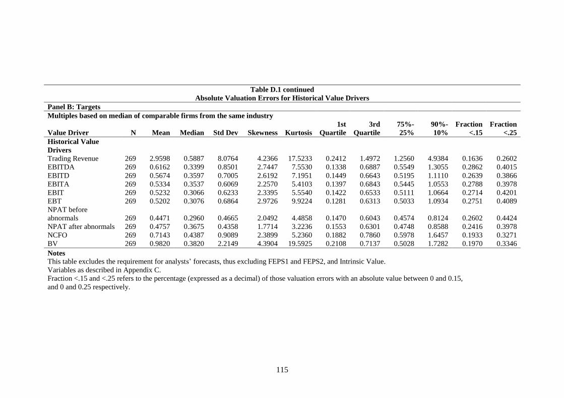
115

Table D.1 continued

Absolute Valuation Errors for Historical Value Drivers

Panel B: Targets

Multiples based on median of comparable firms from the same industry

Value Driver N Mean Median Std Dev Skewness Kurtosis

1st

Quartile

3rd

Quartile

75%-

25%

90%-

10%

Fraction

<.15

Fraction

<.25

Historical Value

Drivers 6 2 3 7 8 9 10 11 12 13 15 16

Trading Revenue 269 2.9598 0.5887 8.0764 4.2366 17.5233 0.2412 1.4972 1.2560 4.9384 0.1636 0.2602

EBITDA 269 0.6162 0.3399 0.8501 2.7447 7.5530 0.1338 0.6887 0.5549 1.3055 0.2862 0.4015

EBITD 269 0.5674 0.3597 0.7005 2.6192 7.1951 0.1449 0.6643 0.5195 1.1110 0.2639 0.3866

EBITA 269 0.5334 0.3537 0.6069 2.2570 5.4103 0.1397 0.6843 0.5445 1.0553 0.2788 0.3978

EBIT 269 0.5232 0.3066 0.6233 2.3395 5.5540 0.1422 0.6533 0.5111 1.0664 0.2714 0.4201

EBT 269 0.5202 0.3076 0.6864 2.9726 9.9224 0.1281 0.6313 0.5033 1.0934 0.2751 0.4089

NPAT before

abnormals 269 0.4471 0.2960 0.4665 2.0492 4.4858 0.1470 0.6043 0.4574 0.8124 0.2602 0.4424

NPAT after abnormals 269 0.4757 0.3675 0.4358 1.7714 3.2236 0.1553 0.6301 0.4748 0.8588 0.2416 0.3978

NCFO 269 0.7143 0.4387 0.9089 2.3899 5.2360 0.1882 0.7860 0.5978 1.6457 0.1933 0.3271

BV 269 0.9820 0.3820 2.2149 4.3904 19.5925 0.2108 0.7137 0.5028 1.7282 0.1970 0.3346

Notes

This table excludes the requirement for analysts’ forecasts, thus excluding FEPS1 and FEPS2, and Intrinsic Value.

Variables as described in Appendix C.

Fraction <.15 and <.25 refers to the percentage (expressed as a decimal) of those valuation errors with an absolute value between 0 and 0.15,

and 0 and 0.25 respectively.

116

Table D.2

Signed Valuation Errors for Historical Value Drivers

Panel A: Acquirers

Multiples based on median of comparable firms from the same industry

Value Driver N Mean Median Std Dev Skewness Kurtosis

1st

Quartile

3rd

Quartile

75%-

25%

90%-

10%

Fraction

<.15

Fraction

<.25

Historical Value

Drivers 6 2 3 7 8 9 10 11 12 13 15 16

Trading Revenue 230 -0.3241 0.1444 1.4112 -2.6689 7.7800 -0.4713 0.4672 0.9385 2.5006 0.1522 0.2522

EBITDA 230 -0.0119 0.0797 0.5194 -1.2270 1.5619 -0.1927 0.3251 0.5178 1.2449 0.3043 0.4565

EBITD 230 -0.0185 0.0844 0.5288 -1.3348 1.8955 -0.1996 0.3300 0.5296 1.2757 0.3087 0.4391

EBITA 230 -0.0461 0.0745 0.5710 -1.6428 3.4621 -0.2618 0.3093 0.5711 1.2253 0.2783 0.4435

EBIT 230 -0.0476 0.0813 0.5842 -1.9074 4.7051 -0.2111 0.2960 0.5071 1.1701 0.2652 0.4435

EBT 230 -0.0824 0.0538 0.5746 -1.7513 3.2986 -0.2474 0.2920 0.5395 1.2380 0.3087 0.4696

NPAT before

abnormals 230 -0.0281 0.0691 0.4984 -1.4387 2.3795 -0.1575 0.2839 0.4414 1.1547 0.3348 0.4783

NPAT after abnormals 230 -0.0240 0.0788 0.5811 -1.3323 2.2188 -0.2259 0.3142 0.5401 1.3107 0.3130 0.4304

NCFO 230 -0.0566 0.0650 0.6587 -1.2291 1.5133 -0.2867 0.4036 0.6903 1.5947 0.2565 0.3913

BV 230 0.1704 0.2235 0.3907 -0.5196 -0.1626 -0.0651 0.4391 0.5042 1.0698 0.2478 0.3957

117

Table D.2 continued

Signed Valuation Errors for Historical Value Drivers

Panel B: Targets

Multiples based on median of comparable firms from the same industry

Value Driver N Mean Median Std Dev Skewness Kurtosis

1st

Quartile

3rd

Quartile

75%-

25%

90%-

10%

Fraction

<.15

Fraction

<.25

Historical Value

Drivers 6 2 3 7 8 9 10 11 12 13 15 16

Trading Revenue 269 -2.6356 -0.2365 8.1883 -4.1690 17.0905 -1.4972 0.2626 1.7598 5.6426 0.1636 0.2602

EBITDA 269 -0.3288 -0.0510 0.9977 -2.1799 5.0603 -0.5355 0.2299 0.7654 1.8794 0.2862 0.4015

EBITD 269 -0.2468 -0.0224 0.8676 -1.9110 4.1618 -0.4860 0.2751 0.7610 1.7144 0.2639 0.3866

EBITA 269 -0.2093 -0.0080 0.7811 -1.5735 2.7762 -0.4725 0.2794 0.7519 1.6807 0.2788 0.3978

EBIT 269 -0.1635 0.0382 0.7978 -1.7432 3.2288 -0.3293 0.3041 0.6334 1.7398 0.2714 0.4201

EBT 269 -0.1449 0.0161 0.8495 -2.2512 6.2936 -0.2982 0.3094 0.6076 1.7815 0.2751 0.4089

NPAT before

abnormals 269 -0.0682 0.0158 0.6431 -1.3935 2.3874 -0.2721 0.3189 0.5910 1.4625 0.2602 0.4424

NPAT after abnormals 269 -0.0295 0.0791 0.6451 -1.1622 1.5021 -0.2758 0.4357 0.7115 1.5198 0.2416 0.3978

NCFO 269 -0.3612 -0.0681 1.0987 -1.8473 3.2254 -0.6110 0.3080 0.9190 2.3152 0.1933 0.3271

BV 269 -0.6306 -0.0293 2.3398 -4.0925 17.5521 -0.5454 0.3223 0.8678 2.3330 0.1970 0.3346

Notes

This table excludes the requirement for analysts’ forecasts, thus excluding FEPS1 and FEPS2, and Intrinsic Value.

Variables as described in Appendix C.

Fraction <.15 and <.25 refers to the percentage (expressed as a decimal) of those valuation errors with an absolute value between 0 and 0.15,

and 0 and 0.25 respectively.

118

Table D.3

Price to Intrinsic Value (P/V) Ratios for Historical Value Drivers

Panel A: Acquirers

Multiples based on median of comparable firms from the same industry

Value Driver N Mean Median Std Dev Skewness Kurtosis

1st

Quartile

3rd

Quartile 75%-25% 90%-10%

Historical Value Drivers 6 2 3 7 8 9 10 11 12 13

Trading Revenue 230 1.6705 1.0624 1.8027 2.4847 6.3085 0.6461 1.9057 1.2596 3.3531

EBITDA 230 1.3203 1.1023 0.7599 1.4415 2.3620 0.7966 1.6215 0.8249 1.6344

EBITD 230 1.3196 1.1316 0.7597 1.4901 2.4310 0.7988 1.6755 0.8767 1.5884

EBITA 230 1.3580 1.1281 0.8004 1.5605 2.5820 0.8369 1.6520 0.8150 1.8154

EBIT 230 1.3315 1.1228 0.7362 1.4640 2.2638 0.8760 1.6230 0.7470 1.6913

EBT 230 1.3905 1.1771 0.7875 1.8129 3.5622 0.9345 1.6283 0.6939 1.5644

NPAT before abnormals 230 1.3078 1.1101 0.6383 1.1314 0.7912 0.9089 1.5762 0.6673 1.6372

NPAT after abnormals 230 1.2554 1.0955 0.6506 0.9978 1.2646 0.8711 1.5740 0.7029 1.5565

NCFO 230 1.3783 1.0852 0.9723 1.5542 2.4739 0.7786 1.7556 0.9770 2.2660

BV 230 1.0678 0.9797 0.5691 0.8867 0.9572 0.6764 1.3895 0.7131 1.3060

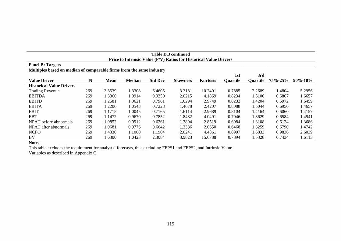
119

Table D.3 continued

Price to Intrinsic Value (P/V) Ratios for Historical Value Drivers

Panel B: Targets

Multiples based on median of comparable firms from the same industry

Value Driver N Mean Median Std Dev Skewness Kurtosis

1st

Quartile

3rd

Quartile 75%-25% 90%-10%

Historical Value Drivers 6 2 3 7 8 9 10 11 12 13

Trading Revenue 269 3.3539 1.3308 6.4605 3.3181 10.2491 0.7885 2.2689 1.4804 5.2956

EBITDA 269 1.3360 1.0914 0.9350 2.0215 4.1869 0.8234 1.5100 0.6867 1.6657

EBITD 269 1.2581 1.0621 0.7961 1.6294 2.9749 0.8232 1.4204 0.5972 1.6459

EBITA 269 1.2206 1.0543 0.7228 1.4678 2.4207 0.8088 1.5044 0.6956 1.4657

EBIT 269 1.1715 1.0045 0.7165 1.6114 2.9689 0.8104 1.4164 0.6060 1.4157

EBT 269 1.1472 0.9670 0.7852 1.8482 4.0491 0.7046 1.3629 0.6584 1.4941

NPAT before abnormals 269 1.0852 0.9912 0.6261 1.3804 2.8519 0.6984 1.3108 0.6124 1.3686

NPAT after abnormals 269 1.0681 0.9776 0.6642 1.2386 2.0650 0.6468 1.3259 0.6790 1.4742

NCFO 269 1.4330 1.1000 1.1904 2.0241 4.4861 0.6997 1.6833 0.9836 2.6039

BV 269 1.6300 1.0423 2.3084 3.9823 15.6788 0.7894 1.5328 0.7434 1.6113

Notes

This table excludes the requirement for analysts’ forecasts, thus excluding FEPS1 and FEPS2, and Intrinsic Value.

Variables as described in Appendix C.

120

Table D.4

Matched Absolute Valuation Errors

Panel A: Acquirers

Multiples based on median of comparable firms from the same industry

Value Driver N Mean Median Std Dev Skewness Kurtosis

1st

Quartile

3rd

Quartile

75%-

25%

90%-

10%

Fraction

<.15

Fraction

<.25

Historical Value

Drivers 6 2 3 7 8 9 10 11 12 13 15 16

Trading Revenue 56 0.5522 0.3990 0.6360 2.5498 6.6713 0.1816 0.6029 0.4213 1.0318 0.2321 0.3214

EBITDA 56 0.2516 0.2004 0.2044 1.3823 2.1008 0.1082 0.3393 0.2310 0.4976 0.3929 0.5893

EBITD 56 0.2684 0.2521 0.2166 1.1725 1.3984 0.0923 0.3815 0.2892 0.5116 0.3929 0.5000

EBITA 56 0.2343 0.1981 0.1650 0.7391 -0.2219 0.1034 0.3571 0.2537 0.4032 0.3750 0.6071

EBIT 56 0.2453 0.1936 0.1807 0.6825 -0.4267 0.1091 0.3492 0.2402 0.5045 0.3571 0.5714

EBT 56 0.2377 0.1629 0.2103 1.4487 1.9239 0.0866 0.3481 0.2615 0.4362 0.4464 0.6071

NPAT before

abnormals 56 0.1941 0.1573 0.1376 0.5939 -0.7861 0.0777 0.2868 0.2091 0.3705 0.4643 0.6964

NPAT after abnormals 56 0.2527 0.2032 0.2165 1.1227 0.6935 0.0829 0.3542 0.2713 0.5242 0.4107 0.6250

NCFO 56 0.3523 0.2515 0.3533 2.4993 7.8568 0.1179 0.5044 0.3865 0.6274 0.3393 0.4821

BV 56 0.3222 0.2996 0.2254 0.8010 -0.1470 0.1587 0.4160 0.2573 0.6626 0.2143 0.4286

Intrinsic Value Driver

Intrinsic Value 56 0.2869 0.1908 0.2341 0.7732 -0.4302 0.0900 0.4688 0.3788 0.5833 0.3750 0.5536

Forecast Value Driver

FEPS1 56 0.2120 0.1360 0.2548 2.6075 7.1796 0.0602 0.2594 0.1992 0.3768 0.5357 0.7321

FEPS2 56 0.1987 0.1267 0.2315 2.7103 7.8836 0.0688 0.2384 0.1696 0.3537 0.5179 0.7500

121

Table D.4 continued

Matched Absolute Valuation Errors

Panel B: Targets

Multiples based on median of comparable firms from the same industry

Value Driver N Mean Median Std Dev Skewness Kurtosis

1st

Quartile

3rd

Quartile

75%-

25%

90%-

10%

Fraction

<.15

Fraction

<.25

Historical Value

Drivers 6 2 3 7 8 9 10 11 12 13 15 16

Trading Revenue 56 0.8366 0.4547 1.1523 2.2911 5.0019 0.1528 0.7857 0.6329 2.2906 0.2321 0.3571

EBITDA 56 0.3315 0.2042 0.5422 4.0294 17.1204 0.0678 0.3758 0.3080 0.4166 0.4107 0.6071

EBITD 56 0.3534 0.2065 0.5717 3.8267 15.4425 0.0906 0.3924 0.3018 0.4761 0.4643 0.5714

EBITA 56 0.2659 0.1663 0.2739 1.9647 4.4501 0.0716 0.3624 0.2908 0.5044 0.4464 0.5893

EBIT 56 0.3651 0.1755 0.5692 3.1086 9.9580 0.0780 0.4058 0.3278 0.5888 0.4464 0.6250

EBT 56 0.3792 0.1724 0.7852 4.5405 20.9648 0.0797 0.3350 0.2553 0.5093 0.4464 0.5714

NPAT before

abnormals 56 0.3241 0.2158 0.4885 3.9646 16.8292 0.1272 0.3015 0.1744 0.5154 0.3214 0.6071

NPAT after abnormals 56 0.3238 0.2145 0.2705 1.0442 0.3713 0.1433 0.5603 0.4171 0.6561 0.3036 0.5357

NCFO 56 0.4526 0.2697 0.6119 2.9984 10.2201 0.1161 0.5256 0.4095 0.8623 0.3036 0.4643

BV 56 0.6080 0.2618 1.1469 3.5190 12.0794 0.0799 0.5674 0.4874 0.8896 0.3393 0.4821

Intrinsic Value Driver

Intrinsic Value 56 0.4640 0.1716 1.0315 4.4837 20.5480 0.0817 0.4029 0.3212 0.6419 0.4643 0.6071

Forecast Value Driver

FEPS1 56 0.2800 0.1758 0.2723 1.9279 3.6664 0.1159 0.3243 0.2084 0.5472 0.4107 0.6429

FEPS2 56 0.2070 0.1546 0.1724 1.6502 3.1997 0.1029 0.2695 0.1666 0.3598 0.4821 0.7321

Notes

FEPS is Forecast Earnings Per Share. The number following relates to the forecast period (FEPS1 is one year ahead Forecast Earnings Per Share).

FEPS based on median analysts’ forecasts are selected.

Other variables as described in Appendix C.

Fraction <.15 and <.25 refers to the percentage (expressed as a decimal) of those valuation errors with an absolute value between 0 and 0.15,

and 0 and 0.25 respectively.

122

Table D.5

Matched Signed Valuation Errors

Panel A: Acquirers

Multiples based on median of comparable firms from the same industry

Value Driver N Mean Median Std Dev Skewness Kurtosis

1st

Quartile

3rd

Quartile

75%-

25%

90%-

10%

Fraction

<.15

Fraction

<.25

Historical Value

Drivers 6 2 3 7 8 9 10 11 12 13 15 16

Trading Revenue 56 -0.0967 0.1321 0.8399 -1.9926 3.9916 -0.2741 0.4646 0.7387 1.6946 0.2321 0.3214

EBITDA 56 0.0412 0.0903 0.3233 -0.7604 1.1860 -0.1416 0.2341 0.3757 0.7502 0.3929 0.5893

EBITD 56 0.0247 0.0626 0.3459 -0.7631 0.6852 -0.1300 0.2599 0.3899 0.8187 0.3929 0.5000

EBITA 56 0.0389 0.0754 0.2857 -0.1856 -0.3377 -0.1572 0.2177 0.3749 0.7357 0.3750 0.6071

EBIT 56 0.0317 0.0607 0.3048 -0.2815 -0.2850 -0.1440 0.2284 0.3724 0.7565 0.3571 0.5714

EBT 56 -0.0052 0.0252 0.3190 -0.9817 1.0188 -0.1421 0.1953 0.3375 0.7312 0.4464 0.6071

NPAT before

abnormals 56 0.0506 0.0513 0.2338 -0.1366 -0.5067 -0.1102 0.2077 0.3179 0.5952 0.4643 0.6964

NPAT after abnormals 56 0.0452 0.0602 0.3314 0.1207 0.4092 -0.1304 0.2057 0.3362 0.7979 0.4107 0.6250

NCFO 56 -0.0073 0.1020 0.5011 -1.7030 4.0133 -0.1691 0.2868 0.4559 1.1521 0.3393 0.4821

BV 56 0.2572 0.2707 0.2986 -0.0054 -0.1788 0.0887 0.4114 0.3227 0.8834 0.2143 0.4286

Intrinsic Value Driver

Intrinsic Value 56 0.1166 0.1558 0.3533 -1.0264 1.2922 -0.0417 0.3708 0.4125 0.6866 0.3750 0.5536

Forecast Value Driver

FEPS1 56 -0.0590 -0.0122 0.3274 -1.8732 4.2856 -0.1429 0.1281 0.2710 0.6254 0.5357 0.7321

FEPS2 56 -0.0220 0.0237 0.3055 -1.9343 4.9739 -0.1167 0.1327 0.2494 0.5088 0.5179 0.7500

123

Table D.5 continued

Matched Signed Valuation Errors

Panel B: Targets

Multiples based on median of comparable firms from the same industry

Value Driver N Mean Median Std Dev Skewness Kurtosis

1st

Quartile

3rd

Quartile

75%-

25%

90%-

10%

Fraction

<.15

Fraction

<.25

Historical Value

Drivers 6 2 3 7 8 9 10 11 12 13 15 16

Trading Revenue 56 -0.5256 -0.0728 1.3263 -1.9086 3.4191 -0.7510 0.2884 1.0394 2.8650 0.2321 0.3571

EBITDA 56 -0.1544 -0.0390 0.6177 -3.3037 12.7668 -0.2364 0.1451 0.3815 0.7670 0.4107 0.6071

EBITD 56 -0.1786 -0.0261 0.6493 -3.1406 11.5453 -0.2888 0.1056 0.3944 0.8085 0.4643 0.5714

EBITA 56 -0.0931 -0.0088 0.3717 -1.2557 1.8734 -0.2565 0.1198 0.3762 0.8622 0.4464 0.5893

EBIT 56 -0.1746 -0.0010 0.6547 -2.5713 7.4802 -0.2456 0.1424 0.3880 0.8574 0.4464 0.6250

EBT 56 -0.1842 0.0154 0.8535 -4.0883 17.9319 -0.2334 0.1571 0.3905 0.8641 0.4464 0.5714

NPAT before

abnormals 56 -0.1330 -0.0186 0.5724 -3.1061 11.6558 -0.2458 0.1830 0.4289 0.7968 0.3214 0.6071

NPAT after abnormals 56 -0.0135 0.0077 0.4240 -0.4089 0.2196 -0.2137 0.2062 0.4199 1.1559 0.3036 0.5357

NCFO 56 -0.2540 -0.0401 0.7193 -2.2828 6.6183 -0.3803 0.1598 0.5401 1.2180 0.3036 0.4643

BV 56 -0.2766 0.0059 1.2704 -3.1809 10.3012 -0.2309 0.2596 0.4905 1.4200 0.3393 0.4821

Intrinsic Value Driver

Intrinsic Value 56 -0.1555 0.0705 1.1219 -4.1623 18.3717 -0.0969 0.2071 0.3040 0.8768 0.4643 0.6071

Forecast Value Driver

FEPS1 56 -0.1447 -0.1274 0.3642 -1.0776 1.3113 -0.2998 0.1008 0.4006 0.8006 0.4107 0.6429

FEPS2 56 -0.0768 -0.0491 0.2595 -0.7653 0.4979 -0.2196 0.1304 0.3501 0.5962 0.4821 0.7321

Notes

FEPS is Forecast Earnings Per Share. The number following relates to the forecast period (FEPS1 is one year ahead Forecast Earnings Per Share).

FEPS based on median analysts’ forecasts are selected.

Other variables as described in Appendix C.

Fraction <.15 and <.25 refers to the percentage (expressed as a decimal) of those valuation errors with an absolute value between 0 and 0.15,

and 0 and 0.25 respectively.

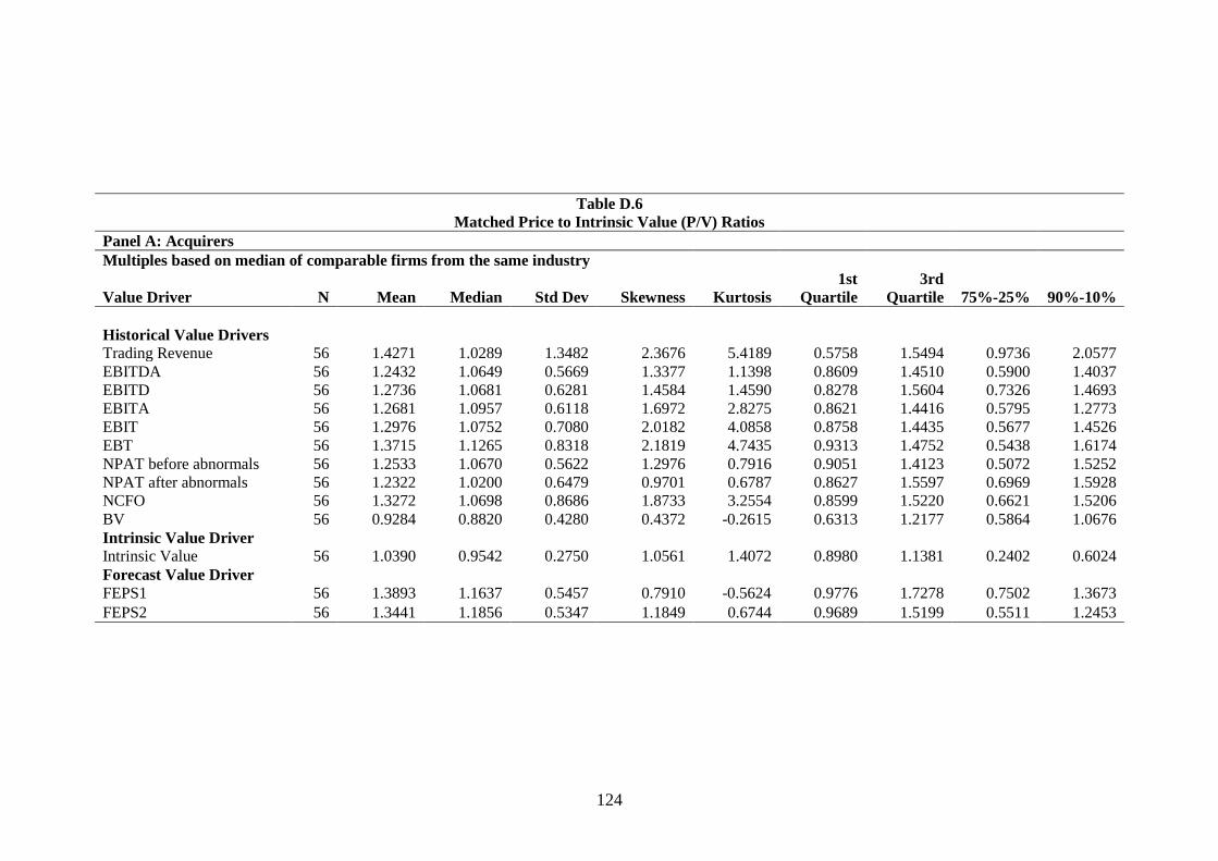
124

Table D.6

Matched Price to Intrinsic Value (P/V) Ratios

Panel A: Acquirers

Multiples based on median of comparable firms from the same industry

Value Driver N Mean Median Std Dev Skewness Kurtosis

1st

Quartile

3rd

Quartile 75%-25% 90%-10%

Historical Value Drivers 6 2 3 7 8 9 10 11 12 13

Trading Revenue 56 1.4271 1.0289 1.3482 2.3676 5.4189 0.5758 1.5494 0.9736 2.0577

EBITDA 56 1.2432 1.0649 0.5669 1.3377 1.1398 0.8609 1.4510 0.5900 1.4037

EBITD 56 1.2736 1.0681 0.6281 1.4584 1.4590 0.8278 1.5604 0.7326 1.4693

EBITA 56 1.2681 1.0957 0.6118 1.6972 2.8275 0.8621 1.4416 0.5795 1.2773

EBIT 56 1.2976 1.0752 0.7080 2.0182 4.0858 0.8758 1.4435 0.5677 1.4526

EBT 56 1.3715 1.1265 0.8318 2.1819 4.7435 0.9313 1.4752 0.5438 1.6174

NPAT before abnormals 56 1.2533 1.0670 0.5622 1.2976 0.7916 0.9051 1.4123 0.5072 1.5252

NPAT after abnormals 56 1.2322 1.0200 0.6479 0.9701 0.6787 0.8627 1.5597 0.6969 1.5928

NCFO 56 1.3272 1.0698 0.8686 1.8733 3.2554 0.8599 1.5220 0.6621 1.5206

BV 56 0.9284 0.8820 0.4280 0.4372 -0.2615 0.6313 1.2177 0.5864 1.0676

Intrinsic Value Driver

Intrinsic Value 56 1.0390 0.9542 0.2750 1.0561 1.4072 0.8980 1.1381 0.2402 0.6024

Forecast Value Driver

FEPS1 56 1.3893 1.1637 0.5457 0.7910 -0.5624 0.9776 1.7278 0.7502 1.3673

FEPS2 56 1.3441 1.1856 0.5347 1.1849 0.6744 0.9689 1.5199 0.5511 1.2453

125

Table D.6 continued

Matched Price to Intrinsic Value (P/V) Ratios

Panel B: Targets

Multiples based on median of comparable firms from the same industry

Value Driver N Mean Median Std Dev Skewness Kurtosis

1st

Quartile

3rd

Quartile 75%-25% 90%-10%

Historical Value Drivers 6 2 3 7 8 9 10 11 12 13

Trading Revenue 56 1.7878 1.1648 1.9231 3.2644 11.8676 0.8287 1.8659 1.0371 2.5706

EBITDA 56 1.2863 1.1113 0.5725 1.6542 2.9322 0.9101 1.4496 0.5395 1.2102

EBITD 56 1.3245 1.1053 0.6030 1.2066 0.9606 0.9075 1.6909 0.7834 1.4192

EBITA 56 1.2763 1.1082 0.5715 1.5289 2.7227 0.9115 1.5612 0.6498 1.2120

EBIT 56 1.3591 1.0816 0.8040 2.0345 4.3895 0.8748 1.5971 0.7223 1.2766

EBT 56 1.3620 1.0764 0.9040 2.9776 10.2050 0.8811 1.4274 0.5463 1.2547

NPAT before abnormals 56 1.3521 1.1060 0.8624 2.8989 9.7785 0.9056 1.5391 0.6335 1.2008

NPAT after abnormals 56 1.2147 1.0904 0.7386 1.5745 2.9188 0.8035 1.4666 0.6631 1.4483

NCFO 56 1.4582 1.2031 0.9449 1.9629 3.8849 0.8748 1.6826 0.8078 1.7656

BV 56 1.4744 0.9933 1.7824 4.0487 16.8796 0.8751 1.3634 0.4883 1.5202

Intrinsic Value Driver

Intrinsic Value 56 1.2577 0.9504 1.2165 4.6608 21.9698 0.8963 1.1613 0.2650 0.7756

Forecast Value Driver

FEPS1 56 1.3484 1.1222 0.6717 1.8407 3.4885 0.9054 1.5779 0.6725 1.3615

FEPS2 56 1.2549 1.0645 0.4882 0.9284 -0.2608 0.8936 1.6677 0.7741 1.1207

Notes

FEPS is Forecast Earnings Per Share. The number following relates to the forecast period (FEPS1 is one year ahead Forecast Earnings Per Share).

FEPS based on median analysts’ forecasts are selected.

Other variables as described in Appendix C.

126

Table D.7

Acquirers Absolute Valuation Errors Using One Year Ahead Market Capitalisation

Multiples based on median of comparable firms from the same industry

Value Driver N Mean Median Std Dev Skewness Kurtosis

1st

Quartile

3rd

Quartile

75%-

25%

90%-

10%

Fractio

n <.15

Fractio

n <.25

Historical Value

Drivers 6 2 3 7 8 9 10 11 12 13 15 16

Trading Revenue 146 0.6569 0.5040 0.7985 3.1100 9.6632 0.2396 0.7116 0.4720 0.7847 0.1370 0.2603

EBITDA 146 0.4349 0.4039 0.2630 0.8250 0.7543 0.2254 0.5926 0.3672 0.6118 0.1233 0.3014

EBITD 146 0.4498 0.4174 0.2856 1.3542 2.8491 0.2554 0.6008 0.3455 0.6231 0.1164 0.2466

EBITA 146 0.4256 0.3908 0.2877 0.8679 0.9700 0.2187 0.5790 0.3603 0.6763 0.1644 0.3014

EBIT 146 0.4407 0.4043 0.2961 1.0822 1.3867 0.2220 0.5818 0.3597 0.6622 0.1575 0.2945

EBT 146 0.4520 0.3814 0.3619 1.9318 4.4216 0.2075 0.5846 0.3771 0.6550 0.1507 0.3356

NPAT before

abnormals 146 0.4185 0.3866 0.2682 0.7504 0.6093 0.2375 0.5947 0.3573 0.6661 0.1849 0.2671

NPAT after abnormals 146 0.4649 0.4217 0.3043 1.2179 2.3713 0.2539 0.6265 0.3725 0.7324 0.1507 0.2466

NCFO 146 0.4939 0.4291 0.3788 1.3303 1.9383 0.1858 0.6479 0.4621 0.7474 0.1986 0.2945

BV 146 0.4550 0.4465 0.2407 0.0522 -1.0714 0.2653 0.6434 0.3780 0.6429 0.1096 0.2397

Intrinsic Value Driver

Intrinsic Value 146 0.4314 0.4029 0.3080 2.0021 6.7837 0.2201 0.5736 0.3534 0.5796 0.1438 0.2945

Forecast Value Driver

FEPS1 146 0.4189 0.3807 0.3560 2.2266 6.8041 0.1767 0.5500 0.3733 0.6570 0.1986 0.3288

FEPS2 146 0.4067 0.3467 0.2893 1.5553 3.2554 0.2111 0.5424 0.3313 0.5670 0.1712 0.3219

Share Price

Current Share Price 146 0.2851 0.2467 0.1993 0.8070 0.1333 0.1264 0.4232 0.2968 0.4929 0.3425 0.5137

Notes

FEPS is Forecast Earnings Per Share. The number following relates to the forecast period (FEPS1 is one year ahead Forecast Earnings Per Share).

FEPS based on median analysts’ forecasts are selected. Other variables as described in Appendix C.

Fraction <.15 and <.25 refers to the percentage (expressed as a decimal) of those valuation errors with an absolute value between 0 and 0.15,

and 0 and 0.25 respectively.

127

Table D.8

Acquirers Absolute Valuation Errors Using Two Year Ahead Market Capitalisation

Multiples based on median of comparable firms from the same industry

Value Driver N Mean Median Std Dev Skewness Kurtosis

1st

Quartile

3rd

Quartile

75%-

25%

90%-

10%

Fractio

n <.15

Fractio

n <.25

Historical Value

Drivers 6 2 3 7 8 9 10 11 12 13 15 16

Trading Revenue 137 0.8776 0.5745 1.5537 4.3804 18.9924 0.3233 0.7600 0.4367 0.7973 0.1022 0.1898

EBITDA 137 0.5577 0.4522 0.4979 2.5801 6.9064 0.3133 0.6216 0.3083 0.6564 0.1095 0.2044

EBITD 137 0.5750 0.4858 0.5562 2.7580 7.8582 0.2812 0.6127 0.3315 0.6506 0.0876 0.1971

EBITA 137 0.5500 0.4646 0.5232 2.9976 10.2920 0.2724 0.6505 0.3780 0.6817 0.1387 0.2117

EBIT 137 0.5761 0.4864 0.5933 3.2804 12.1728 0.2613 0.6327 0.3714 0.6742 0.1314 0.2190

EBT 137 0.5822 0.4317 0.6549 3.3920 12.7132 0.2675 0.6635 0.3959 0.6674 0.1241 0.2336

NPAT before

abnormals 137 0.5277 0.4567 0.5053 3.2089 12.0944 0.2691 0.6167 0.3476 0.6601 0.1314 0.2409

NPAT after abnormals 137 0.5826 0.4871 0.5958 3.2883 12.1004 0.2628 0.6605 0.3977 0.7736 0.1095 0.2263

NCFO 137 0.6439 0.5022 0.6660 2.9805 10.1782 0.3114 0.7092 0.3978 1.1047 0.1387 0.1971

BV 137 0.5309 0.4817 0.3170 1.1917 2.5100 0.3004 0.6932 0.3928 0.7104 0.1022 0.1606

Intrinsic Value Driver

Intrinsic Value 137 0.6587 0.4582 1.2468 5.2451 27.3416 0.2763 0.6264 0.3501 0.7208 0.1460 0.2409

Forecast Value Driver

FEPS1 137 0.7203 0.4521 1.3087 4.8212 23.7512 0.2677 0.6395 0.3718 0.8278 0.1460 0.2336

FEPS2 137 0.6795 0.4384 1.1229 4.6794 22.4039 0.2982 0.6339 0.3357 0.6645 0.0803 0.2044

Share Price

Current Share Price 137 0.4517 0.3592 0.4073 2.2897 6.2199 0.2110 0.5480 0.3370 0.6578 0.1752 0.3066

Notes

FEPS is Forecast Earnings Per Share. The number following relates to the forecast period (FEPS1 is one year ahead Forecast Earnings Per Share).

FEPS based on median analysts’ forecasts are selected. Other variables as described in Appendix C.

Fraction <.15 and <.25 refers to the percentage (expressed as a decimal) of those valuation errors with an absolute value between 0 and 0.15,

and 0 and 0.25 respectively.

128

Table D.9

Acquirers Absolute Valuation Errors Using Three Year Ahead Market Capitalisation

Multiples based on median of comparable firms from the same industry

Value Driver N Mean Median Std Dev Skewness Kurtosis

1st

Quartile

3rd

Quartile

75%-

25%

90%-

10%

Fractio

n <.15

Fractio

n <.25

Historical Value

Drivers 6 2 3 7 8 9 10 11 12 13 15 16

Trading Revenue 125 0.8101 0.6116 0.9208 3.3192 11.1213 0.3831 0.7910 0.4079 0.7468 0.0320 0.1360

EBITDA 125 0.5851 0.5219 0.5201 3.3198 12.9560 0.3526 0.6813 0.3287 0.6507 0.0880 0.1760

EBITD 125 0.5924 0.4966 0.5452 3.2119 11.8613 0.3010 0.6981 0.3971 0.6664 0.0960 0.1840

EBITA 125 0.5867 0.5184 0.5489 3.4683 13.5688 0.2864 0.6776 0.3912 0.6526 0.0800 0.1920

EBIT 125 0.5849 0.5087 0.5454 3.1983 12.0700 0.2908 0.6743 0.3835 0.6768 0.0960 0.2080

EBT 125 0.5990 0.5067 0.5485 3.1763 11.6467 0.3321 0.6760 0.3439 0.6132 0.0640 0.2080

NPAT before

abnormals 125 0.5739 0.5046 0.4829 3.3812 14.0404 0.3386 0.6851 0.3464 0.6347 0.0960 0.1440

NPAT after abnormals 125 0.5851 0.5498 0.4362 2.4080 7.9798 0.3474 0.7090 0.3616 0.7538 0.1280 0.1520

NCFO 125 0.6452 0.5823 0.5388 2.6069 8.0515 0.3417 0.7181 0.3764 0.7495 0.0960 0.1520

BV 125 0.5872 0.5463 0.3597 1.6821 4.4806 0.3720 0.7372 0.3652 0.6844 0.0640 0.1440

Intrinsic Value Driver

Intrinsic Value 125 0.6571 0.5237 0.8674 4.2874 18.5089 0.3096 0.6942 0.3846 0.6829 0.0800 0.1840

Forecast Value Driver

FEPS1 125 0.9166 0.4850 2.2117 5.1648 25.8370 0.2898 0.6833 0.3935 1.0140 0.1120 0.1920

FEPS2 125 0.9114 0.4844 2.2514 5.1870 25.9862 0.3131 0.6526 0.3394 0.6904 0.0960 0.2000

Share Price

Current Share Price 125 0.5228 0.4184 0.5576 3.2988 11.9695 0.2467 0.6111 0.3644 0.6525 0.1600 0.2640

Notes

FEPS is Forecast Earnings Per Share. The number following relates to the forecast period (FEPS1 is one year ahead Forecast Earnings Per Share).

FEPS based on median analysts’ forecasts are selected. Other variables as described in Appendix C.

Fraction <.15 and <.25 refers to the percentage (expressed as a decimal) of those valuation errors with an absolute value between 0 and 0.15,

and 0 and 0.25 respectively.

129