mix-design of a novel semi-transparent layer for solar roads
TRANSCRIPT
HAL Id: tel-03162227https://tel.archives-ouvertes.fr/tel-03162227
Submitted on 8 Mar 2021
HAL is a multi-disciplinary open accessarchive for the deposit and dissemination of sci-entific research documents, whether they are pub-lished or not. The documents may come fromteaching and research institutions in France orabroad, or from public or private research centers.
L’archive ouverte pluridisciplinaire HAL, estdestinée au dépôt et à la diffusion de documentsscientifiques de niveau recherche, publiés ou non,émanant des établissements d’enseignement et derecherche français ou étrangers, des laboratoirespublics ou privés.
Mix-design of a novel semi-transparent layer for solarroads
Domenico Vizzari
To cite this version:Domenico Vizzari. Mix-design of a novel semi-transparent layer for solar roads. Civil Engineering.École centrale de Nantes, 2020. English. �NNT : 2020ECDN0023�. �tel-03162227�

THESE DE DOCTORAT DE
L'ÉCOLE CENTRALE DE NANTES
ECOLE DOCTORALE N° 602
Sciences pour l'Ingénieur
Spécialité : Génie Civil
Mix-design of a novel semi-transparent layer for solar roads Thèse présentée et soutenue à Nantes, le 22 octobre 2020 Unité de recherche : Département Matériaux et Structures (MAST-MIT) de l’Université Gustave Eiffel
Par
Domenico VIZZARI
Rapporteurs avant soutenance : Virginie Mouillet, Directrice de recherche, CEREMA, Aix en Provence; Christiane Raab, Professeure, Technical University of Darmstadt (Allemagne).
Composition du Jury :
Président : Frederic Grondin Professeur des universités, École Centrale de Nantes; Examinateurs : Jean Dumoulin Chargé de recherche, Université Gustave Eiffel, Bouguenais;
Massimo Losa Professeur, University of Pisa (Italie); Pedro Partal Professeur, Universidad de Huelva (Espagne).
Dir. de thèse : Emmanuel Chailleux Directeur de recherche, Université Gustave Eiffel, Bouguenais; Co-encadrant : Eric Gennesseaux Ingénieur des TPE, Université Gustave Eiffel, Bouguenais.


Summary List of Figures .................................................................................................................................... 7
List of Tables ..................................................................................................................................... 9
Acknowledgments.......................................................................................................................... 11
Funding ............................................................................................................................................ 12
Introduction ........................................................................................................................................ 13
The goal ............................................................................................................................................ 14
Thesis structure ............................................................................................................................... 14
1. Literature review: road pavement energy harvesting technologies ..................................... 17
1.1 Photovoltaic road ................................................................................................................ 18
1.2 Hybrid road (COP21 prototype) ...................................................................................... 20
1.2.1 Sensecity prototype ........................................................................................................ 21
1.3 Solar thermal systems ........................................................................................................ 23
1.3.1 Asphalt solar collectors .................................................................................................. 23
1.3.2 Porous layer as solar thermal system ............................................................................ 25
1.3.3 A 2-D hydrothermal model ........................................................................................... 25
1.3.4 FEM model of porous layer as solar thermal system ..................................................... 26
1.3.5 Air-Powered Energy-Harvesting Pavement ................................................................. 28
1.4 Heat pipes ............................................................................................................................ 29
1.5 Thermoelectric generators (TEGs) ................................................................................... 30
1.6 Piezoelectric pavement ...................................................................................................... 31
1.7 Comparison ......................................................................................................................... 34
1.7.1 Observations based on the literature review ................................................................. 38
1.8 Conclusions ......................................................................................................................... 38
2. Materials and methods ................................................................................................................. 39
2.1 Polyurethane ....................................................................................................................... 39
2.1.1 What is the polyurethane ............................................................................................... 39
2.1.2 Microstructure of a polyurethane .................................................................................. 41
2.1.3 Definition of curing ....................................................................................................... 42
2.1.4 Introduction to polymer aging mechanisms .................................................................. 42
2.1.5 Applications of polyurethanes ....................................................................................... 43
2.1.6 Requirements for a solar road ........................................................................................ 44
2.2 Mix design methods ........................................................................................................... 45
4
2.2.1 Particle packing degree .................................................................................................. 45
2.2.2 The surface dressing ...................................................................................................... 50
2.2.3 The factorial design ....................................................................................................... 51
2.3 Conclusions ......................................................................................................................... 52
3. Polymerization and viscoelastic behavior of the polyurethane according to curing
temperature ......................................................................................................................................... 55
3.1 Presentation of the materials: the thermoset polyurethanes ........................................ 55
3.2 Viscoelastic characterization of the polyurethane ......................................................... 59
3.2.1 Basics of viscoelastic characterization ........................................................................... 59
3.2.2 Experimental plan ......................................................................................................... 61
3.2.3 Procedure used to determine the curing time of the polyurethanes .............................. 62
3.3 Curing kinetic ...................................................................................................................... 64
3.3.1 Effect of the temperature on the curing kinetic ............................................................. 64
3.3.2 Repeatability of the DSR procedure to measure the curing kinetic of the
polyurethanes… ............................................................................................................................ 65
3.3.3 The curing time of the polyurethanes ............................................................................ 66
3.3.4 Modeling the curing time through the Arrhenius law .................................................. 67
3.4 The effect of the curing temperature at achieved polymerization .............................. 69
3.4.1 Preliminary tests: effect of storage time ........................................................................ 69
3.4.2 Complex modulus vs temperature for the frequency of 1 Hz ........................................ 69
3.4.3 Curing temperature effect on mechanical properties ..................................................... 71
3.4.4 Modeling the polyurethane based on generalized Maxwell........................................... 73
3.4.5 Discussion ..................................................................................................................... 77
3.5 Conclusions ......................................................................................................................... 78
4. The semi-transparent layer design ............................................................................................. 81
4.1 The glass aggregates .......................................................................................................... 81
4.2 Procedure for the manufacture of the semi-transparent layer ..................................... 82
4.3 Evaluation of the mechanical performance: the three-point bending test ................. 83
4.4 Evaluation of the optical performance: the power loss ................................................. 85
4.4.1 Novel approach modeling the intensity-voltage curve .................................................. 87
4.4.2 Validation ...................................................................................................................... 89
4.5 Preliminary Mix-design of the semi-transparent layer based on the particle packing
degree (STL1). ................................................................................................................................. 90

5
4.5.1 Mechanical performance ................................................................................................ 90
4.5.2 Optical performance ...................................................................................................... 92
4.6 Mix-design of the semi-transparent layer based on the fraction factorial design
(STL2). .............................................................................................................................................. 94
4.6.1 Optical performance ...................................................................................................... 96
4.6.2 Mechanical Performance ............................................................................................... 97
4.6.3 Skid Resistance .............................................................................................................. 99
4.6.4 The Optimal Mixture .................................................................................................. 100
4.7 Mix design of the semi-transparent layer based on the surface dressing treatment
(STL3). ............................................................................................................................................ 100
4.7.1 Determination of the optimum glue content ............................................................... 102
4.7.2 Optical performance, toughness and skid resistance ................................................... 104
4.8 Conclusions ....................................................................................................................... 105
5. Aging of polyurethane ............................................................................................................... 107
5.1 Photodegradation of polyurethane ................................................................................ 107
5.2 Materials ............................................................................................................................ 109
5.3 Aging condition ................................................................................................................ 110
5.4 FTIR: Fourier transformer infrared spectroscopy ........................................................ 111
5.4.1 FTIR spectra of fresh glues .......................................................................................... 113
5.4.2 FTIR spectra of aged glues .......................................................................................... 115
5.5 DSC: Differential scanning calorimetric test ................................................................. 118
5.5.1 Aging effect on the glass transition temperature detected by means of the DSC ........ 121
5.6 Rotational rheometer test: Linear domain determination .......................................... 123
5.7 Complex modulus measurements ................................................................................. 125
5.8 Discussion .......................................................................................................................... 129
5.9 Aging of the semi-transparent layer .............................................................................. 130
5.10 Conclusions ....................................................................................................................... 133
General conclusions ........................................................................................................................ 135
Perspectives ................................................................................................................................... 139
Résumé long .................................................................................................................................. 140
Perspectives ................................................................................................................................... 145
References ......................................................................................................................................... 147
Annex ................................................................................................................................................. 157
6
1: The principles of the photovoltaic effect ............................................................................... 157
2: The intensity-voltage curve of a solar cell............................................................................. 158
3: Pyranometer .............................................................................................................................. 159
4: Introduction to the prototype ................................................................................................. 161
The semi-transparent layer.......................................................................................................... 161
The electrical layer ....................................................................................................................... 162
The porous concrete layer ............................................................................................................ 162
The base layer .............................................................................................................................. 163
5: Types of surface dressing ........................................................................................................ 163
Single chip seal ............................................................................................................................ 163
Double chip seal ........................................................................................................................... 163
Racked-in chip seal ...................................................................................................................... 164
Cape seal. ..................................................................................................................................... 164
Sandwich chip seal ...................................................................................................................... 164
Inverted chip seal ......................................................................................................................... 164
5: The British pendulum test ....................................................................................................... 165
6: Plots of E’, E’’ and tan(δ) according to generalized Maxwell for the glue B, C and D ... 167
7: FTIR of glue B ............................................................................................................................ 172
8: FTIR of glue D ........................................................................................................................... 173
9: Strain sweep glue B .................................................................................................................. 174
10: Strain sweep glue C ................................................................................................................ 174
11: Strain sweep glue D ............................................................................................................... 175
12: Frequency sweep of the glue B ............................................................................................. 176
13: Frequency sweep of the glue C ............................................................................................. 177
14: Frequency sweep of the glue D ............................................................................................ 179
7
List of Figures Figure 1. Energy harvesting through the road pavement. ........................................................... 17
Figure 2. Exploded view of a photovoltaic road [12] .................................................................... 18
Figure 3. Examples of photovoltaic roads. ...................................................................................... 20
Figure 4. Sensecity prototype [21]. ................................................................................................... 21
Figure 5. Measurements on the solar road – 1st of May [21]. ....................................................... 22
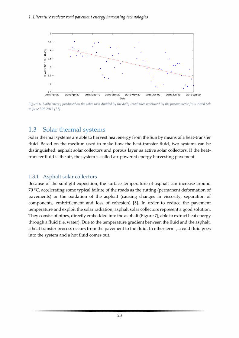
Figure 6. Daily energy produced by the solar road divided by the daily irradiance measured
by the pyranometer from April 6th to June 30th 2016 [21]. ........................................................... 23
Figure 7. Layer of solar collectors along a road section [11]......................................................... 24
Figure 8. Schematic diagram of fluid circulation at saturation and laboratory prototype [26].
............................................................................................................................................................... 25
Figure 9. Effect of the porosity and of the irradiance on the efficiency of the system [27]. ..... 26
Figure 10. Sectional view of the FEM model and the interactions with the environment [29].
............................................................................................................................................................... 27
Figure 11. Rendered three-dimensional model of an Air-Powered Energy-Harvesting
Pavement [31] ...................................................................................................................................... 28
Figure 12. Schematic principle of the heat pipe system built in Germany [34]. ........................ 29
Figure 13. Operating principle of a thermoelectric generator applied to a road infrastructure
[41]. ....................................................................................................................................................... 31
Figure 14. Piezoelectric effect [42]. ................................................................................................... 31
Figure 15. Reaction of diisocyanate with polyol [61]..................................................................... 39
Figure 16. A simple representation of a polyurethane [62]. ......................................................... 40
Figure 17. Hydrogen bonding between segments in urethane groups [71]. .............................. 41
Figure 18. Photodegradation cycle for polymers [78]. .................................................................. 43
Figure 19. Schematic representation of the wall effect and the loosening effect [93]. .............. 46
Figure 20. Wall effect due to the container [93]. ............................................................................. 49
Figure 21. Polyurea reaction [121]. ................................................................................................... 57
Figure 22. Formula of the polyamines, also called polyaspartic acid derivatives [122]. .......... 57
Figure 23. A simple representation of a DSR in oscillation mode [127]. .................................... 60
Figure 24. Schematic representation of the DMA performed on a cylinder of bitumen [129]. 61
Figure 25. Experimental plan. ........................................................................................................... 62
Figure 26. Procedure to measure the rheological parameters during the polymerization. ..... 63
Figure 27. Procedure to evaluate the evolution of the shear complex modulus applied the
glue A, cured at 10°C. ........................................................................................................................ 63
Figure 28. Evolution of the phase angle δ and of complex shear modulus |G*| during the
polymerization for the glue A at three different curing temperature. ........................................ 64
Figure 29. Repeatability for the DSC procedure to measure the curing kinetic of the
polyurethanes...................................................................................................................................... 65
Figure 30. Criteria for evaluation of the curing time (The plot refers to the polyurethane B at
the 18 temperature of 30°C).. ............................................................................................................ 66
Figure 31. Modeling experimental data according to the Arrhenius law. ................................. 68
Figure 32. Evolution of |E*| during the storage time for glue A. ............................................... 69
Figure 33. Complex modulus vs temperature for different polyurethanes cured at 50 °C. .... 70

8
Figure 34. Complex modulus |E for different curing temperatures at frequency of 1Hz. ...... 72
Figure 35. Comparison between the Black curve of a typical bitumen and the Black curves of
2 polyurethanes. a: curing at 50 °C; b: curing at 30 °C; c: curing at 10 °C. ................................. 73
Figure 36. Generalized Maxwell [143]. ............................................................................................ 74
Figure 37. Modeling of E’, E’’ and tan(δ) according to generalized Maxwell for the glue A. . 76
Figure 38. Grading curves of the glass fractions. ........................................................................... 81
Figure 39. Manufacture of STL1 and STL2. .................................................................................... 82
Figure 40. The three-point flexural test. .......................................................................................... 83
Figure 41. Bending of a generalized beam [148]. ........................................................................... 84
Figure 42. Example of stress-strain curve. ...................................................................................... 85
Figure 43. Example of intensity-voltage curve. .............................................................................. 86
Figure 44. Modeling of the power curves. ...................................................................................... 89
Figure 45. Sketch of the bond between glass and glue. ................................................................. 91
Figure 46. Influence of the glue content on the toughness of mix γ............................................ 92
Figure 47. Effect of glue content and thickness on the power loss. ............................................. 93
Figure 48. Influence of each mix-design variable on the power loss. ......................................... 97
Figure 49. Influence of each mix-design variable on the toughness. .......................................... 99
Figure 50. Device for the aggregate spreading. ............................................................................ 101
Figure 51. Square vs hexagonal lattice [162]. ................................................................................ 102
Figure 52. Aggregates spread on a white surface. ....................................................................... 103
Figure 53. Formation of hydroperoxide. ....................................................................................... 108
Figure 54. Comparison of generic polyurethane and polyurea [175]. ...................................... 110
Figure 55. Right: natural aging; left: sunlight simulator ............................................................. 110
Figure 56. Equivalence between natural and accelerated aging. ............................................... 111
Figure 57. Transmission mode vs ATR mode [179]. .................................................................... 112
Figure 58. Wavenumber vs penetration depth of the polyurethane. ........................................ 113
Figure 59. FTIR of fresh glues. ........................................................................................................ 113
Figure 60. Normalized FTIR spectra of fresh glues in the range 4000-2000 cm-1. ................... 114
Figure 61. Normalized FTIR spectra of fresh glues in the range 2000-400 cm-1. ...................... 114
Figure 62. FTIR spectra of glue A after aging in the range 2000-4000 cm-1. ............................. 116
Figure 63. FTIR spectra of glue A after aging in the range 2000-400 cm-1. ............................... 116
Figure 64. FTIR spectra of glue C after aging in the range 4000-2000 cm-1. .............................. 117
Figure 65. FTIR spectra of glue C after aging in the range 2000-600 cm-1. ................................ 118
Figure 66. Example of differential scanning calorimeter [186]. ................................................. 119
Figure 67. Tg (glass transition temperature), Tc (crystallization temperature) and Tm
(melting temperature) in DSC measurement [189]. ..................................................................... 120
Figure 68. Different methods to calculate the Tg [191]. .............................................................. 121
Figure 69. Days of UV exposition vs Tg detected by the DSC. .................................................. 122
Figure 70. DSC curves measured at different aging time for the glue A. ................................. 123
Figure 71. Procedure for the strain sweep. ................................................................................... 124
Figure 72. Strain sweep of glue A. ................................................................................................. 124
Figure 73. Procedure for the frequency sweep. ............................................................................ 125
Figure 74. tan(δ) vs Temperature at different aging time for the glue A. ................................ 126

9
Figure 75. Days of UV exposition vs Tg detected by the rotational rheometer test at the
frequency of 0.01Hz. ........................................................................................................................ 127
Figure 76. Shear complex modulus vs temperature for the glue C for the frequency of 0.01
Hz. ....................................................................................................................................................... 127
Figure 77. Frequency sweep of the glue A at - 10°C, for different aging time. ........................ 128
Figure 78. Frequency sweep of the glue A at 20°C, for different aging time. .......................... 128
Figure 79. Frequency sweep of the glue A at 60°C, for different aging time. .......................... 129
Figure 80. Evolution of the power loss of STL1. .......................................................................... 131
Figure 81. Evolution of power loss of STL3. ................................................................................. 132
Figure 82. The photovoltaic effect [199]. ....................................................................................... 157
Figure 83. Example of intensity-voltage curve (black line) and power curve (red line). ....... 158
Figure 84. Schematic representation of a pyranometer [202].. ................................................... 159
Figure 85. Sketch of the prototype. ................................................................................................ 161
Figure 86. Example of British pendulum test [209]. .................................................................... 165
List of Tables Table 1. List of companies which worked on photovoltaic roads. .............................................. 20
Table 2. List of companies which worked on piezoelectric pavement. ...................................... 33
Table 3. Positives, negatives and optimization criteria for road energy harvesting systems. . 36
Table 4. Cost, energy output, efficiency and TRL for different road energy harvesting
systems. *Assuming : 100 cymbals per m2, 100 vehicle per hour ................................................ 37
Table 5. Types of polyurethanes. ...................................................................................................... 44
Table 6. Main properties of the polyurethanes used for this study. ........................................... 56
Table 7. Chemical composition of the polyurethanes. .................................................................. 59
Table 8. Curing time of the polyurethanes at different temperatures based on four criteria. . 67
Table 9. Δ and E values of the Arrhenius law. ............................................................................... 68
Table 10. Complex modulus at 1 Hz and 20°C for each glue, at different curing temperatures.
............................................................................................................................................................... 72
Table 11. Glass transition temperature at different curing temperature. ................................... 77
Table 12. Parameters of the model to fit the intensity-voltage curves. ....................................... 89
Table 13. Mix design for the STL1. ................................................................................................... 90
Table 14. Effect of the type of glue on the mechanical performance of the semi-transparent
layer. ..................................................................................................................................................... 91
Table 15. Effect of the grading curve on the mechanical performance of the semi-transparent
layer. ..................................................................................................................................................... 92
Table 16. Effect of the type of glue on the power loss. .................................................................. 93
Table 17. Experimental domain of the variables. ........................................................................... 94
Table 18. Model matrix ...................................................................................................................... 95
Table 19. Mix-design of each experiment. ....................................................................................... 95
Table 20. Vector y ̅ containing the value of power loss measured for each mix. ....................... 96
Table 21. Mix-design to minimize the power loss of the semi-transparent layer. .................... 97
Table 22. Vector y containing the value of toughness measured for each mix. ......................... 98
10
Table 23. Mix-design to maximize the toughness of the semi-transparent layer. ..................... 98
Table 24. Values of BPN for the mixtures of Table 19. .................................................................. 99
Table 25. Optimal mix-design for both mechanical and optical performances. ...................... 100
Table 26. Aggregate spreading density for different glass fractions. ........................................ 101
Table 27. Surface dressing for different glass fractions. .............................................................. 103
Table 28. Power loss and BPN for different types of polyurethane. ......................................... 105
Table 29. Evolution of Tg because of aging, detected by the DSC. ........................................... 122
Table 30. Evolution of Tg because aging, detected by the rotational rheometer test at the
frequency of 1Hz. ............................................................................................................................. 126
Table 31. Evolution of Tg because aging, detected by the rotational rheometer test at the
frequency of 0.01Hz. ........................................................................................................................ 126
Table 32. Power loss difference between time 14 and time 0 for STL1. .................................... 131
Table 33. Power loss difference between time 12 and time 0 for STL3. .................................... 132
Table 34. Skid resistance specifications [156]................................................................................ 166

11
Acknowledgments When I moved in Nantes it was raining. I had two big luggage, no umbrella and a jacket that
seemed to absorb water. The only available place was the room of an old Lady and I spent one
week eating frozen foods and looking for new accommodations. After a few days, I already
missed my family, my friends and my land. I was almost ready to go back home, but at the
same time I didn't want to give up so easily.
My first day at IFSTTAR I was nervous and excited at the same time. In front of the gate, Eric
and Stephane were waiting for me. I didn’t expect any particular welcome, instead I found
very nice people, who answered to all my questions smiling. Within a few hours, I was already
formally part of the MIT laboratory. I signed my contract, I had my own laptop and a
welcoming office! Therefore, I met Emmanuel Chailleux, my supervisor. All day long, he
explained the project that he had in mind and he showed me the whole laboratory! My first
impression was of a passionate, curious and rigorous researcher. I was not wrong! In the next
days, I met the other researchers, technicians and PhD students and in less than one week I
had changed my mind: maybe that place wasn’t that bad!
Three years have passed since that day. During this time, I had the opportunity to learn a lot,
make some mistakes and grow and develop as a person. This manuscript is the perfect
opportunity to thank all the people who helped and supported me along this way.
Firstly, I want to express my gratitude for my parents. I hope they are proud of me, at least the
half as I’m proud of them!
I would like to thank again Emmanuel Chailleux for his inspiring guidance and
encouragement throughout the PhD, as well as for always being friendly and helpful. I extend
my thanks to Stephane Lavaud and Eric Gennesseaux for their good advices and proficient
discussions.
Acknowledgements must be done to all the researchers and technicians of MIT and LAME, in
particular Stephane Bouron for all the time spend together between samples, pv cells and cans
of glue, Nadège Vignard for the dynamic mechanical analysis, Gille Didilet for the three-point
bending tests and Jacques Kerveillant “pour les cours de français ’’.
Thanks to all my colleagues, I share with you many good times. Thanks to Ibishola for your
contagious and positive attitude. Thanks to Natasha for your help and friendship. Thanks to
Justine to “stend me” in the office for all this time! Thanks to Thomas, Talita, Pravin, Rodrigo,
Amelie, Brahim and Shreedhar. Before being excellent colleagues, you are very good friends.
Thanks to Davide Lo Presti and Ana Jiménez del Barco Carrión for involving me in SMARTI
ETN. I had the opportunity to travel around the world, make new experiences and enjoy good
times with all the other fellows.
I would like to thank Prof Pedro Partal and his research group for the secondment in Huelva.
It was a great experience and I learnt a lot.
Thanks also to Prof Praticò for all the precious advices since I left the University Mediterranea.

12
Acknowledgements for all the jury. It is a pleasure to submit my research at your attention.
Special thanks to my girlfriend Laura. You have always supported me, especially in the most
difficult moments.
I also want to thanks my friends in Italy, you are the worst and the best friends I could ask!
Probably I forget someone, I say sorry for that. Acknowledgements could continue, I have
many memories with each of you. I need to write a second manuscript for that!
Funding The research presented in this manuscript is part of SMARTI ETN. SMARTI ETN project and
received funding from the European Union’s Horizon 2020 Programme under the Marie
Skłodowska-Curie actions for research, technological development and demonstration, under
grant n.721493.

Introduction The world energy consumption is constantly increasing. According to the International Energy
Outlook 2017, the energy consumption will increase from 575 quadrillion Btu1 in 2015 to 736
quadrillion Btu in 2040. Petroleum and other liquids remain the largest source of energy (33%
in 2015) and, unfortunately, a great source of pollution. As it is well-known, fossil fuels use
reject high level of carbon dioxide in the atmosphere, accelerating the greenhouse effect and
causing climate change. In this scenario, renewable energies play an important role,
representing a possible solution for the next future. Today the “clean energy” represents
around 19.2% of the global demand and it is divided in 8.9% from traditional biomass, 4.2%
from biomass/geothermal/solar heat, 3.9% from hydropower, 1.4% from wind/solar power
and 0.8% from biofuel. [1]
Among the sources of energy, the Sun is by far the largest. The solar constant, which represents
the solar flux intercepted by the earth, is 1.37 kW/m2. Considering that part of the solar flux is
scattered and absorbed by the atmosphere and the clouds, the average flux striking the earth
surface is 174.7 W/m2. Integrating it over the whole earth’s surface, the potential power of the
Sun is 89300 TW. In other terms, the use of this power for just 2 hours could cover the
worldwide energy consumption of one year [2]!
At the current state, this energy is directly exploitable in two ways: by solar thermal systems
and photovoltaic effect.
The solar thermal systems are able to collect and/or concentrate the solar radiation from the
Sun by means of water or molten salts. They are used as active solar heating for personal use
or implemented in thermal power plant, where the steam, obtained by the water, is used to
activate turbines. In 2015, the energy produced by this mean was 435 GW, plus 37.2 GW thanks
to the new installed systems in 2015. However the market has suffered a decline of 14% in
comparison with 2014. This bad result was due to the shrinking markets in China and Europe
[1].
The solar cells generate electricity thanks to the photovoltaic effect. The use of this technology
is growing rapidly, with a plus 25% in 2016, equivalent to 75 GW. Currently the total power
generation is 301 GW and China is the leader in terms of cumulative installed capacity (78.1
GW), followed by Japan (42.8 GW), Germany (41.3 GW) and US (40.3 GW), while the largest
increment in 2016 were recorded in China (34.5 GW) and US (14.7 GW) [1].
Furthermore, the average photovoltaic module selling prices have decreased by more than
two orders of magnitude in 40 years and, by the end of 2018, the global average module selling
price was below $0.25/W.2 For example, electricity prices of other sources as fossil fuels and
nuclear fission have remained relatively constant over a long period. By contrast, PV cells
prices have decreased sharply. The result of declining costs of PV cells is a reduction of
electricity price [3, 4].
1 Btu is the British Thermal Unit, equivalent to 1055 Joule

Introduction
14
The world of road engineering could seems excluded by this “solar revolution”, which is a
mistake. In reality, there is a widespread research, which suggests new solutions to exploit the
solar radiation. One should just consider that the road network is exposed to a big amount of
sunlight, reaching in summertime values up to 40 MJ/m2 over the course of a day [5]. For
example, in France the average Global Horizontal Irradiance3 (GHI) is 1274.1 KWh/m2 per year
[6]. Considering that the road network in France is around 1 million of km and assuming that
the average width of the road section is 6 m, the result is a surface of 6000 km2, which could
intercept 7644.6 TWh of Sun energy in one year. Just to have an idea of the order of magnitude,
the total energy demand in France is 475 TWh per year [7]! If this amount of energy could be
effectively used, it would mark a revolution.
In prospective, it is possible to imagine a road network not only as a transportation system for
people and goods, but also as a technology able to generate electricity exploiting existing
surfaces. The use of existing transportation infrastructures for energy harvesting may avoid to
occupy new lands, which could be exploited for other purposes (agriculture, industry etc.) or
to preserve the biodiversity in some special areas.
The goal The main goal of this PhD thesis is to contribute to the road engineering, in particular in the
field of the energy harvesting technologies. At this scope, a novel road energy harvesting
system is presented. The idea is to develop and design materials and structure from a
pavement point of view, taking into account durability as well energy efficiency. The core of
this research is the optimization of a semi-transparent layer for surface courses used in a
prototype of hybrid solar pavement collector. This hybrid system has been already
conceptualized (see Chapter 1.2) but still need development to be implemented at full scale.
Thesis structure The thesis starts with a general review of the road systems able to harvest energy, making a
comparison in terms of initial cost, electrical output, efficiency and technology readiness level.
The idea is to move from the results and the observations of other researchers and, on their
basis, define the thesis objectives.
To assist the reader in a better understanding of the manuscript, the literature review is
enriched with a brief introduction about the polyurethane, which is used as binder in the
manufacture of the semi-transparent layer. Furthermore, the basics of the packing density
methods, the surface dressing and the factorial design are presented. These
methods/techniques will be applied for the mix-design of the semi-transparent layer.
The third chapter is dedicated to the characterization of the polyurethane in terms of curing
kinetic and of viscoelastic behavior. More in detail, an experimental campaign was conducted
3 It is the total solar radiation incident on a horizontal surface

Introduction
15
on four thermoset polyurethanes, performing two types of tests: the Dynamic Mechanical
Analysis and the Dynamic Shear Rheometer.
The fourth chapter deals with the mix-design of the semi-transparent layer, a novel mixture
made of glass aggregates bonded together through the polyurethane. The top layer plays a
fundamental role because it has to support the traffic load, guarantee the vehicle friction, allow
the passage of the sunlight and protect the solar cells. For this reason, the mixture has been
optimized in terms of optical and mechanical performances.
The semi-transparent layer is also exposed to the weather changes, which could affect the
material and in particular the binder. For this reason, the fifth chapter focuses on the aging of
the polyurethane. The objective is to understand the evolution of the binder in terms of
chemical and mechanical behavior, by performing the Fourier Transformer Infrared
Spectroscopy, the Differential Scanning Calorimeter and the Rotational Rheometer test.
Furthermore, the semi-transparent layer has been exposed for more than one year to the
weather changes and its optical performance has been monitored monthly.
The last chapter is dedicated to the conclusions. The main results are highlighted and
presented. These observations are “breeding grown” for further research, in the perspective of
a full scale application of the system.

1. Literature review: road pavement energy harvesting technologies
17
1. Literature review: road pavement energy harvesting
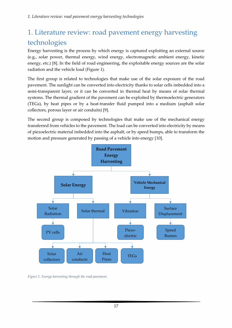
technologies Energy harvesting is the process by which energy is captured exploiting an external source
(e.g., solar power, thermal energy, wind energy, electromagnetic ambient energy, kinetic
energy, etc.) [8]. In the field of road engineering, the exploitable energy sources are the solar
radiation and the vehicle load (Figure 1).
The first group is related to technologies that make use of the solar exposure of the road
pavement. The sunlight can be converted into electricity thanks to solar cells imbedded into a
semi-transparent layer, or it can be converted in thermal heat by means of solar thermal
systems. The thermal gradient of the pavement can be exploited by thermoelectric generators
(TEGs), by heat pipes or by a heat-transfer fluid pumped into a medium (asphalt solar
collectors, porous layer or air conduits) [9].
The second group is composed by technologies that make use of the mechanical energy
transferred from vehicles to the pavement. The load can be converted into electricity by means
of piezoelectric material imbedded into the asphalt, or by speed bumps, able to transform the
motion and pressure generated by passing of a vehicle into energy [10].
Figure 1. Energy harvesting through the road pavement.
Road Pavement
Energy
Harvesting
Solar Energy Vehicle Mechanical
Energy
Solar
Radiation Solar thermal Vibration
Surface
Displacement
PV cells
Solar
collectors
Air
conducts
Heat
Pipes TEGs
Piezo-
electric
Speed
Bumps

1. Literature review: road pavement energy harvesting technologies
18
1.1 Photovoltaic road A photovoltaic road aims at converting the sunlight in electricity thanks to the solar cells
placed under a semi-transparent layer. The general design of a photovoltaic road consists of
three principal layers (Figure 2): the top element is a semi-transparent layer made of tempered
glass, polymer or glass aggregates bounded together using a special resin (i.e. epoxy,
polyurethane etc.). The semi-transparent layer plays a fundamental role because it has to
support the traffic load, ensure safe driving thanks to adequate adherence condition, allow the
passage of the sunlight to the solar cells and protect the electronic component; the second
element is the electric layer where the solar cells are located and the last element is the base
layer which has to transmit the traffic load to the pavement, subgrade or base structure [11].
Figure 2. Exploded view of a photovoltaic road [12]
In academia, Northmore and Tighe [12] proposed a sandwich structure composed by two
laminated 10mm tick panes of tempered glass for the transparent layer, 12.7 mm and 19.1 mm
thick panes of Glass fiber Polyester GPO-3 (a fiberglass laminate consisting of polyester resin
reinforced with fiberglass mat base for applications up to 155°C with good thermal,
mechanical and electrical properties [13]) for the electrical and the base layer respectively. In
terms of mechanical performance, the photovoltaic road was able to support a stress of
16.6 MPa, which was the endurance limit4 of the fiberglass foil.
Dezfooli et al [14] proposed two different prototypes in order to evaluate the feasibility of the
photovoltaic roads. The first prototype is composed of a top layer in polycarbonate for the
transmission of sunlight, a second layer contains the solar cells and finally an aluminum plate
used to keep the layers together. The second prototype is composed of four parts: an asphalt
layer to withstand the traffic load, the solar cells enclosed between two rubber layers and the
top porous layer to drain and channel the water and to protect the solar cells. Based on the
results of the flexural bending test, the first prototype was able to support 600 KPa before the
failure.
Ma et al [15] designed a photovoltaic floor, where the solar cells, enclosed by two EVA
(Ethylene Vinyl Acetate) /PVB (Polyvinyl Butyral) foils, are sandwiched between anti-slip
front tempered glass and rear support tempered glass. The total front size is 500×500 mm and
the thickness is about 20 mm. In each floor tile, 9 mono-crystalline silicon solar cells are
4 Also called “fatigue limit”, it is the stress level below which failure doesn’t occur
1. Literature review: road pavement energy harvesting technologies
19
connected in series, generating an electrical power of 30-40 Wp 5 and ensuring an efficiency of
15%. The maximum compressive strength for the photovoltaic floor was around 15-16 MPa.
Comparing the three solutions, the tempered glasses of Northmore et al. and Ma et al. seem to
be adapted to support the traffic load, which is around 1 MPa for a heavy truck. The
disadvantage of these systems is that they are all prefabricated structures, whose application
in full scale could be complex and expensive.
Photovoltaic roads also attracted industry attention (Figure 3). The Table 1 lists the principal
companies, which built full scale prototypes:
COMPANY DESCRIPTION ELECTRICAL
OUTPUT APPLICATIONS
Solar
Roadways
[16]
They proposed a hexagonal panel
of around 0.4 m2 composed by an
electrical layer (containing the
solar cells) enclosed between two
layers of tempered glass
hermetically sealed. Furthermore
some LED lights are imbedded
into the pavement to make road
lines and signage
44 Wh per
panel
Wattway
[17]
Colas company designed panels
containing 15-cm wide
polycrystalline silicon cells that
transform solar energy into
electricity. The cells are coated in a
multilayer substrate composed by
resins and polymers, translucent
enough to allow the passage of the
sunlight, and resistant enough to
withstand truck traffic
20 m2 + 1000
sun-hour/year
to provide
energy for an
average single
French
household
• A parking lot of 50 m2
in Vendéspace (Roche-
sur-Yon) able to
produce 6300
KWh/year
• 50 m2 of panels have
been installed at the
Georgia Visitor
Information Center,
producing 7000
KWh/year
• 1 km of Wattway road
have been installed in
Normandy, producing
280 MWh/year
Solaroad
[18]
The technology consists of
concrete modules of 2.5 - 3.5
meters with a translucent top layer
of tempered glass, which is about
1 cm thick. The top layer has to be
translucent for sunlight and repel
dirt as much as possible. At the
3500
KWh/year per
module
• A bike path of 72
meters built in
Krommenie
(Netherland) which
produces 70 KWh/m2
per year
5 It is the Watt-peak and it represents the maximum power supplied by a solar cell in standard conditions

1. Literature review: road pavement energy harvesting technologies
20
same time, it must be skid
resistant and strong enough in
order to guarantee a safety drive
Qilu
transportation
[19]
The structure is typical of a solar
road: semi-transparent layer + pv
cells + base layer
460 Wh/m2
• A road of 1 km (5875
m2) built in Jinan
(China), able to
produce 1 GWh/year
Table 1. List of companies which worked on photovoltaic roads.
Comparing the photovoltaic roads developed by industry, the solution of Wattway seems to
be the easiest to install, because the panel can be directly placed on existing pavements.
Regarding the electrical output, a correct comparison is not feasible because the data provided
by the companies are not obtained following a standard procedure (i.e. irradiance of 1000
Wh/m2 and temperature of 25°C). Furthermore, phenomena such as the reduction of the
efficiency of the pv cells at high temperatures, aging of the top layer and presence of dirt or
dust are not taking into account for the calculation of the electrical power.
Figure 3. Examples of photovoltaic roads.
1.2 Hybrid road (COP21 prototype) Researchers of IFSTTAR showed growing interest for photovoltaic road and, in occasion of the
COP21 (Conference of Paris - 2015), they presented a novel prototype of “hybrid solar road”.
The system was composed by a semi-transparent layer of 1 cm thick, a porous asphalt layer of
10 cm thick and a pv cell placed between the two layers [20]. The design was based on previous
researches concerning the porous layer as solar thermal system (see chapter 1.3).
The semi-transparent layer was obtained by mixing together recycled glass aggregates with a
transparent binder. Initially, three types of binders have been characterized: i) transparent
bitumen; ii) bio binder and iii) epoxy. Comparing the transmission spectra, the bio binder had
the best characteristics. Unfortunately, bio binder and transparent bitumen require high
temperatures for their application and they could damage the solar cells. For this reason, the
epoxy has been chosen for the manufacture of the top layer.
In general, the semi-transparent layer was treated as an asphalt mixture. The binder content
was around 5% and it was optimized in order to obtain a certain fluidity of the mixture and to
Solar roadways Wattway Solaroad Quilu transportation

1. Literature review: road pavement energy harvesting technologies
21
give a satisfying visual aspect of entire grain surface coating without any visible binder
leakage.
Once the mix-design was defined, the optical performance of the semi-transparent layer has
been tested. In particular, the power loss of the solar cell because of the semi-transparent layer
has been measured. The results showed that the power loss of the mixture having 1 cm thick
was around 52.9%. Furthermore, the reduction of optical performance was detected by
exposing the sample to the weather changes. The power loss moved from 52.9% to 71.7%.
In terms of mechanical performance, a static load has been applied on a sample composed by
the semi-transparent layer stuck on a concrete slab of 7 cm thick. The charging area had a
diameter of 44 mm. The charging force was transmitted to the sample surface via a hard rubber
interface extracted from utilized tires. The sample withstood to 9500N, which is equivalent to
6.25 MPa of compression stress. Considering that the maximum stress of a heavy truck on a
road pavement is around 1 MPa, the result was satisfactory.
1.2.1 Sensecity prototype
In 2016, a big scale experimental mounting of a solar road was installed in the site of the
SenseCity experimental platform located in Marne-la-Vallée near Paris. The installation was
representative of real urban conditions involving partial shading from adjacent building, trees
and masts and can be circulated by pedestrian, bicycles and light vehicles. The system was
constructed on a 195x85cm concrete slab and it consisted of three parallel connected PV panels
of 60 W each covered by 1 cm of semi-transparent layer designed in IFSTTAR (Figure 4) [21].
Figure 4. Sensecity prototype [21].
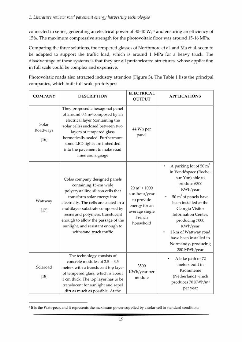
The electrical power (see Annexes 1 and 2) of the prototype and the global irradiance was
measured for 2 months from 6:30 am to 6:30 pm. The Figure 5 is an example of measurements
obtained on the 1st of May 2016. The upper part represents the produced PV electric power in
blue, the global irradiance measured by the pyranometer6 (see Annex 3) Solems RG-100
6 It is a device able to measure the global irradiance (direct + diffuse sunlight)
1. Literature review: road pavement energy harvesting technologies
22
reference cell in green and the global irradiance measured by an SPN1 pyranometer installed
on a 10-meter mast near the solar road, in magenta.
The lower part of Figure 5 refers to the efficiency of the prototype, given by the ratio between
the electric power and the irradiance received by the RG100. The measurements refer to an
area of 1 m2 and they are around 8% between 10:00 am and 2:00 pm.
Figure 5. Measurements on the solar road – 1st of May [21].
Observing the trend of the efficiency curve, there is a decrease between 10 am and 1 pm, which
is certainly due to the heating of the solar cells.
Before 8:15 am, both the prototype and the pyranometer Solems RG-100 were shaded by the
building and the tree on the east. After that, the sun started shining on the sensor again (as
seen through the large jump in the green curve), and progressively, the 3 modules of the solar
road became partially to fully exposed to the sunshine. This progression is seen through the 3
main steps in the blue curve between 8:30 and 10:30 am. Between 11:30 and 12:00 am, the 10
meters mast overshadowed the solar road. Symmetrical effects occurred at sunset.
The maximum power obtained during the measurements was 160 Wh and it was reached
between 10:00 am and 2:00 pm during a sunny day.
Figure 6 shows the ratio between electric produced energy and the irradiation detected by the
pyranometer, around noon (10:00 am – 2:00 pm). It is a pseudo conversion efficiency because
the irradiance received by the solar road is affected by many shadowed period while the
pyranometer is not affected. Anyhow, the figure clearly shows a degradation of the solar cells
performance. This declining tendency is due to the aging of the epoxy and dirt accumulation.
1. Literature review: road pavement energy harvesting technologies
23
Figure 6. Daily energy produced by the solar road divided by the daily irradiance measured by the pyranometer from April 6th
to June 30th 2016 [21].
1.3 Solar thermal systems Solar thermal systems are able to harvest heat energy from the Sun by means of a heat-transfer
fluid. Based on the medium used to make flow the heat-transfer fluid, two systems can be
distinguished: asphalt solar collectors and porous layer as active solar collectors. If the heat-
transfer fluid is the air, the system is called air-powered energy harvesting pavement.
1.3.1 Asphalt solar collectors
Because of the sunlight exposition, the surface temperature of asphalt can increase around
70 °C, accelerating some typical failure of the roads as the rutting (permanent deformation of
pavements) or the oxidation of the asphalt (causing changes in viscosity, separation of
components, embrittlement and loss of cohesion) [5]. In order to reduce the pavement
temperature and exploit the solar radiation, asphalt solar collectors represent a good solution.
They consist of pipes, directly embedded into the asphalt (Figure 7), able to extract heat energy
through a fluid (i.e. water). Due to the temperature gradient between the fluid and the asphalt,
a heat transfer process occurs from the pavement to the fluid. In other terms, a cold fluid goes
into the system and a hot fluid comes out.

1. Literature review: road pavement energy harvesting technologies
24
Figure 7. Layer of solar collectors along a road section [11].
The energy obtained from the asphalt solar collectors could be used for snow melting systems
or for the heating system of the adjacent buildings. The solar collectors can also be embedded
in concrete pavements, but they are less performant because the concrete’s solar absorption
coefficient is lower than asphalt.
The energy balance of an asphalt solar collector involves the following materials and media: i)
the asphalt pavement, ii) the pipes, iii) the air of the atmosphere and iv) the fluid flowing
through the pipes network. In terms of heat exchange mechanisms, the energy is firstly
balanced along the interface between pavement and atmosphere. In this case, the heat flux is
caused by the incident solar radiation, by the convection between asphalt and air and by the
thermal radiation of the asphalt. In return, the heat flux causes a change of temperature in the
pavement, leading to a conduction process from the surface to the interior of the road. The
conduction continues in the interface asphalt-pipe and finally a convection mechanism occurs
in the interface pipe-fluid.
The first application of asphalt solar collectors dates back to 1990 with SERSO project [22]. The
pipes network was installed along a bridge in Swiss, which was part of the national highway.
The idea was to store the excess of heat energy during summer thanks to a heat pump and
reuse the heat in order to melt the snow or the ice during the winter.
Compared to other road energy harvesting systems, the asphalt solar collectors have reached
the highest level of improvement, becoming a quite common technology with a lot of
applications in operational environment. For example, ICAX company designed a pipes
network that use water as heat-transfer fluid [23]. The heat energy is stored in a heat store
constructed beneath the insulated foundation of the buildings around. OOMS [24], a Dutch
company, designed a system for the extraction of cold water from a specific underground
storage medium (in the Netherlands often an aquifer). The water is transported through pipes
in the upper part of the asphalt layers of the pavement and, thanks to the heat exchange, the
water gets warm. Via a heat exchanger, the heat is transported into another underground
reservoir (the so-called hot store) and held at this location until required. In winter, the system
operates in the opposite way.

1. Literature review: road pavement energy harvesting technologies
25
1.3.2 Porous layer as solar thermal system
A multi-layer asphalt pavement for energy harvesting is a sandwich structure able to exploit
the harvested energy for de-freezing the road surface during winter. The first prototype
proposed by IFSTTAR and CEREMA was a de-freezing system inspired by the asphalt solar
collectors. In this system, the tubes were replaced by a draining asphalt through which a heat-
transfer fluid circulated via gravity. The prototype has been evaluated in terms of durability,
stain behavior, water permeability and thermal effectiveness. Furthermore, two types of
porous layers have been tested: a conventional porous asphalt and an asphalt with
polyurethane binder having 22.5% and 30% of porosity, respectively. The results showed a
better mechanical performance for the second asphalt [25].
1.3.3 A 2-D hydrothermal model
In 2016, Asfour et al [26] developed a 2D thermo-hydraulic model to simulate the thermal heat
exchanges of a fluid circulating in a bonding porous layer (Figure 8). The pavement was
composed of a porous asphalt enclosed between a wearing and a base layer. The authors
assumed a stationary hydraulic regime, transient thermic solicitations and that the hydraulic
parameters are independent of temperature. Once the model was defined, a sensitivity
analysis of the temperature at the pavement surface has been conducted. The results
highlighted that the surface temperature is mostly affected by the hydraulic conductivity of
the porous asphalt layer, the fluid injection temperature and the fluid calorific capacity.
Figure 8. Schematic diagram of fluid circulation at saturation and laboratory prototype [26].
The hydraulic conductivity has been measured experimentally by means of a laboratory mock-
up. The mock-up was composed of a wearing course layer of asphalt concrete having 0.06 m
thick; a bonding course layer of 0/14 porous asphalt 0.08 m thick and a base layer of asphalt
concrete 0.05 m thick. The hydraulic conductivity was 2.2 cm/s, for a porosity of 20% and a
slant of 1%.
At the same time, Pascual-Muñoz et al [27] from the Cantabria University worked on a
multilayered solar collector at lab scale. The prototype had dimensions 40*26*9 cm3 and it was
composed by three layers: i) a gap-graded asphalt mixture having 2 cm thick; ii) a porous
asphalt mixture having 4 cm thick and iii) a dense-graded asphalt mixture having 4 cm thick.

1. Literature review: road pavement energy harvesting technologies
26
The authors tested two types of porous asphalt concrete with 23 and 27% of porosity and two
different configurations: saturated and not-saturated porous layer.
The first configuration has been rejected because the water filtered across the top layer. For
this reason all the tests have been conducted in not-saturated condition.
Unlike the prototype of Asfour et al, the water was not put back in circulation by a pump, but
it was a continuous flow coming from a tap. The hydraulic gradient between the inlet and the
outlet of the system was maintained constant thanks to an inlet tank, which was able to release
the overflow by a hole located at a certain height.
The solar radiation was simulated by a lamp of 300 W, which generated an irradiance of 300,
370 or 440 W/m2. The results showed that the hydraulic conductivity across the porous layer
can be significantly improved by increasing the porosity.
Figure 9. Effect of the porosity and of the irradiance on the efficiency of the system [27].
The authors measured the collected energy and they observed that the lower is the hydraulic
conductivity (and consequently the porosity), the more difficult it is for the fluid to collect
energy. In terms of efficiency, defined as the ratio between the energy transferred to the fluid
and the energy absorbed by the surface, it was higher than 0.75 when the porosity is 27%,
instead it dropped to 0.4 when the porosity was 23% (Figure 9). In perspective, they concluded
that the harvested energy could be increased by maximizing the porosity of the middle layer
or by increasing the slope of the system.
1.3.4 FEM model of porous layer as solar thermal system
In 2017, Le Touz et al [28, 29] developed a multi-physics FEM model of multi-layer asphalt
pavement for energy harvesting. The system is composed by a semi-transparent (or an asphalt
mixture called “opaque”) waterproof layer; a porous layer containing a fluid which flows

1. Literature review: road pavement energy harvesting technologies
27
along the width of the road via gravity thanks to the imposed slope; an underlying and a base
layer both opaque and waterproof (Figure 10). The model combines thermal diffusion,
hydraulic convection and radiative transfer.
The structure is subjected to convective exchange with the air, radiative exchange with the sky
and solar radiation. The depth is supposed to be large enough in order to neglect all the
thermal exchanges except at the surface.
Regarding the hydraulic convection, the hypothesis are that the flow of the fluid is stationary,
low and uniform and that the porous layer is in saturated condition; while, for the radiative
transfer, blackbody emissions at ambient temperature for main wavelengths of solar radiation
can be neglected.
The authors coupled the three models in order to compute the temperature field in the
structure and derive the harvested energy.
Figure 10. Sectional view of the FEM model and the interactions with the environment [29].
The harvested energy is given by the formula:
𝐸 = ∫ 𝜌𝑓𝐶𝑝,𝑓𝑢𝑆(𝑇𝑓,𝑜𝑢𝑡 − 𝑇𝑓,𝑖𝑛)+𝑑𝑡
𝑡
1
Where:
- ρf is the density of the fluid (kg/m3);
- Cp is the heat capacity (J/Kg*K);
- u = 1*10-4 is the Darcy velocity (m/s);
- S is the section of the flow (m2);
- (Tf,out - Tf,in)+ is the temperature fluid raise between input and output (K);
- t is the time (s).

1. Literature review: road pavement energy harvesting technologies
28
Considering a length of the flow of 4 m, the harvested energy per m2 was calculated for
different location in France from May to October.
The efficiency of the system is given by the ratio between the harvested energy (Eq. 3) and the
total solar irradiation. In the case of the opaque surface (asphalt mixture), the efficiency ranges
between 31.1% and 41% based on the location. Using the semi-transparent surface, the solar
radiation can penetrate deeply in the structure and the efficiency increases of about 7 % by
reference to the incident radiation.
1.3.5 Air-Powered Energy-Harvesting Pavement
The heat fluid in the asphalt solar collectors is essential to extract energy from the pavements.
However, the presence of a crack in the pipes could compromise all the system, releasing the
fluid and risking the failure of the pavement. The idea proposed by Chiarelli and Garcia [30,
31] is to imbed into the pavement a series of conduits, using the air as heat fluid. The air
conduits are connected to an updraft and a downdraft chimney and, because of the difference
of temperature between the environment and the asphalt, a difference of pressure exists
between the end of the chimney and the entrance into the pavement (Figure 11).
Figure 11. Rendered three-dimensional model of an Air-Powered Energy-Harvesting Pavement [31]
The result is a continuous airflow, which can cool the pavement down during the summer or
heat it up during the winter up to 10% of the initial temperature.
First results on a lab scale prototype demonstrated the feasibility of the system and highlighted
that:
- the lowest surface temperature along with the highest air speed is obtained installing
the pipes in a single row under the pavement wearing course;
- the pipes can be replaced with concrete corrugations, but they reduce the harvested
energy;
- the dimension of the chimney affects the final performance of the system. For this
reason an optimal design is needed; the air flow of the prototype is around 0.58 m/s,
not enough for electricity production.

1. Literature review: road pavement energy harvesting technologies
29
1.4 Heat pipes A heat pipe is a system able to transfer thermal energy quickly. It is sealed at both ends and it
is lined with a wicking material [11]. At certain pressure and temperature, the system reaches
the equilibrium between liquid and vapor state of the fluid enclosed in the pipe.
In particular, the internal liquid (into the wicking material) absorbs thermal energy from the
pipe surface and it evaporates. Pressure forces move the vapor from the hot to the cold part of
the pipe, where it releases the heat, condensing back into liquid. Finally, the capillary action
from the wicking structure transports the liquid back and the cycle starts again [32, 33].
The heat pipes have been applied as snow-melting system, using CO2 as heat-transfer fluid.
Evaporated warm CO2 rises to the top of the heat pipe exploiting a geothermal heat sources.
Once the CO2 reaches the surface, it condenses releasing the heat. After that, the CO2 returns
to the vaporization zone of the heat pipe in liquid state, triggering an automatic cycle. The
result is a heat pipe system able to melt the snow on the pavement without using any external
energy [34].
In 1984, Nydahl proposed a heat pipe system using ammonia for de-icing a bridge in
Wyoming. The diameter of the tubes was of 16 mm and the used material was the black iron
[35].
Recently a system was built in Bad Waldsee (Germany) to cover the entrance of a fire station
along a surface of 165 m2. The pipes have a diameter of 16 mm and they are connected to the
surface through a shaft distribution system (Figure 12). The pipes converge in 5 boreholes at
the depth of 50-75 m in order to study the differences of performances based on different pipes
lengths [34]. In general, shorter is the distance of the pipes from the shaft the more efficient is
heat system.
Figure 12. Schematic principle of the heat pipe system built in Germany [34].
1. Literature review: road pavement energy harvesting technologies
30
In 2017, Liu et al [36] proposed a multi-objective optimization and a thermal simulation of a
snow-melting system. The authors studied the influence of pipes embedded spacing,
embedded depth and wind velocity on the total heating time for the melting process (THT)
and on the lost energy rate absorbed by the environment (LER). Based on the results, the THT
can be decreased by reducing the embedded spacing, the embedded depth and the wind
velocity. On the contrary, the LER can be decreased by increasing the embedded depth and
reducing the embedded spacing and the wind velocity. The optimum (lowest THT and LE) is
given by an embedded spacing of 0.1 m, an embedded depth of 0.06 m and absence of wind.
1.5 Thermoelectric generators (TEGs) Thermoelectric generators (TEGs) produce electricity thanks to the Seebeck effect [37]. They
are composed by thermoelectric couples consisting of n-type (containing free electrons) and p-
type (containing free holes). In semiconductors, charge carriers have the ability to move freely
while carrying charge as well as heat. In the presence of a temperature gradient, the charge
carriers diffuse from the hot side to the cold side. The result is a net charge (negative for
electrons and positive for holes) at the cold side, which produces an electrostatic potential
(voltage). The voltage depends on the difference of temperature between the cold and the hot
side, according to the Eq. 2:
𝑉 = 𝛼∆𝑇 2
Where: α (μV/K) is the Seebeck coefficient and ΔT (K) is the difference of temperature. For
standard thermocouples, α ranges between 8 and 60 μV/K [38].
TEGs have been applied in road engineering as pavement-cooling system. For example,
Hasebe et al. [39] proposed to install a thermoelectric generator coupled with an asphalt solar
collector. The heat-transfer fluid is the water coming from a source (i.e. a river or a lake) near
the road. The water, circulating along the pipe network, is able to absorb heat from the
pavement. Because of the heat, the temperature of the water increases and it is pumped in the
hot side of the TEG. In return, the other side of the TEG is cooled down by the river water.
Thanks to the temperature gap between the hot and the cold side, electrical power is generated
(Figure 13). More in detail, for a ΔT of 15°C, the generated electrical power is around 0.3W.

1. Literature review: road pavement energy harvesting technologies
31
Figure 13. Operating principle of a thermoelectric generator applied to a road infrastructure [41].
In 2012, Wu and Yu [40] built a prototype able to harvest energy thanks to the temperature
difference between the pavement surface and the subgrade soil. The prototype was composed
by an aluminium plate and a rod installed in a hole, drilled along an asphalt sample. A TEG
module was installed on the aluminium plate, using a conductive epoxy as interface. The other
end of the rod was placed on dry sand, in order to simulate the subgrade soil.
The experiment was to simulate the solar energy through a filament lamp and measure the
electrical power. Once the lamp was open, the TEG was able to generate a voltage of 300 mV.
The potential of TEGs was assessed by Guo et al [41]. The authors calculated an electrical
power of 55GWh per day, which could be generated if the entire road network of Florida was
equipped with TEGs.
1.6 Piezoelectric pavement In piezoelectric crystals, when a mechanical strain is applied to the material by an external
stress tension (b), or compression (c), an electric charge occurs on the surfaces (Figure 14).
Figure 14. Piezoelectric effect [42].
Typical piezoelectric natural materials are quartz and amazonite, while barium titanite, lead
titanite and lead zirconate titanite are artificial crystals.
1. Literature review: road pavement energy harvesting technologies
32
Piezo-electric crystals can be imbedded into the pavement, for example along the interface
between surface and binder course. When the vehicle (or the pedestrian) moves over the road,
the wheel generates a pressure on the crystals. In return, the crystal undergoes a deformation,
generating the electric charge [42, 43].
The energy produced by an external stress is given by the Eq. 3 [44]:
𝑈𝐸 =1
2𝑉02휀𝑟𝑡휀0𝐴
𝑡
3
Where:
- UE (J) is the electric energy storage in the piezoelectric device;
- V0 (V) is the electric potential in open circuit;
- A (m2) is the area of the piezoelectric crystal;
- t (m) is the thickness of the piezoelectric crystal;
- εr (dim) is the relative dielectric constant piezoelectric crystal (is a parameter that
indicates how easily a material can become polarized because of an electric field);
- ε0 (F/m) is the dielectric constant in vacuum piezoelectric crystal;
In 2013, Sun et al [45] designed, based on a FEM analysis, a piezoelectric unit having
dimensions 280*280*20 mm3. Each unit is composed by 64 piezoelectric vibrators and it can
generate 0.25 W of electrical power at 15Hz of load frequency, for a load of 0.7 MPa. The
simulation showed that the system can harvest 1.785 MW on each lane and per kilometer.
In 2016, Xiong et al [46] presented a novel piezoelectric energy harvester (PEH). The system
consists of piezoceramic disks sealed in a protective package. Six prototypes were fabricated
and installed in a real road in order to evaluate the feasibility of the system. The average
electrical power of each PEH is 3.106 mW, considering that only 14.43% of the vehicles load
was transmitted to the piezoelectric materials.
At the same time, Moure et al [47] developed some piezoelectric cymbals having 29 mm
diameter. The best configuration was given by 3 cymbals connected in series in a row
transverse to the wheel movement. The system was integrated directly in the asphalt and,
based on the results, each unit was able to generate an electrical power up to 16 µW when a
truck wheel passed on the cymbal. Furthermore, the authors estimated that 30000 cymbals
along a road of 100 m could generate an electrical power of 65 MWh per year.
Not only the academia, but also the industry has shown some interest in this technology, as
highlighted in the table below:
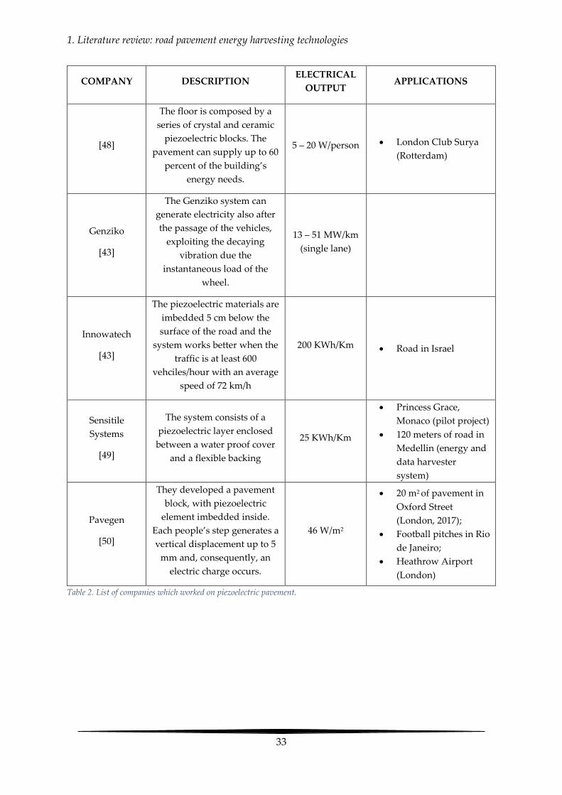
1. Literature review: road pavement energy harvesting technologies
33
COMPANY DESCRIPTION ELECTRICAL
OUTPUT APPLICATIONS
[48]
The floor is composed by a
series of crystal and ceramic
piezoelectric blocks. The
pavement can supply up to 60
percent of the building’s
energy needs.
5 – 20 W/person London Club Surya
(Rotterdam)
Genziko
[43]
The Genziko system can
generate electricity also after
the passage of the vehicles,
exploiting the decaying
vibration due the
instantaneous load of the
wheel.
13 – 51 MW/km
(single lane)
Innowatech
[43]
The piezoelectric materials are
imbedded 5 cm below the
surface of the road and the
system works better when the
traffic is at least 600
vehciles/hour with an average
speed of 72 km/h
200 KWh/Km Road in Israel
Sensitile
Systems
[49]
The system consists of a
piezoelectric layer enclosed
between a water proof cover
and a flexible backing
25 KWh/Km
Princess Grace,
Monaco (pilot project)
120 meters of road in
Medellin (energy and
data harvester
system)
Pavegen
[50]
They developed a pavement
block, with piezoelectric
element imbedded inside.
Each people’s step generates a
vertical displacement up to 5
mm and, consequently, an
electric charge occurs.
46 W/m2
20 m2 of pavement in
Oxford Street
(London, 2017);
Football pitches in Rio
de Janeiro;
Heathrow Airport
(London)
Table 2. List of companies which worked on piezoelectric pavement.

1. Literature review: road pavement energy harvesting technologies
34
1.7 Comparison Each road energy harvesting system has positives, negatives and specific conditions to exploit
the most of their potential in terms of energy output. At this scope, a comparison has been
carried out in Table 3:
Technology Positives Negatives Optimization criteria
Photovoltaic road
Producing electricity
thanks to the solar
cells
Not invasive (some
system are posed on
existing roads)
Dependent on the
sunlight radiation
Low friction of the
glass surface
Aging of top surface
At high temperatures,
the solar cells lose
efficiency
Maximize the
exposure to sunlight
Increase the
transparency of the
top surface
Increase the efficiency
of the solar cells
Asphalt solar
collectors
Providing hot water
Snow-melting system
Reducing Urban Heat
Island (UHI)
Increasing expected
life of the pavement
(lowering the
temperature of the
asphalt during the
summer and raising it
during the winter)
Interference of the
pipes with pavement
performance
Presence of air voids
between pipes and
mixture
All pipes need to be
interconnected and if
one is broken, fluid
could damage the
asphalt
Increasing the Albedo7
of the surface
Increasing the specific
heat capacity of
materials
Reducing the
interference of the
pipes with the asphalt
Porous layer as
solar thermal
system
Providing hot water
Snow-melting system
Low strength of the
porous layer
Low permeability of
the asphalt mixture
Improving the
permeability to
increase the harvested
energy
Using of semi-
transparent layer to
maximize the heat
7 It is the fraction of the incident sunlight reflected from a surface. Mathematically, it is given by the ratio between
the reflected light and the incident light. For instance, the albedo of a black body is 0, while the albedo of fresh
deep snow is 0.9

1. Literature review: road pavement energy harvesting technologies
35
transfer to the porous
layer
Air-Powered
Energy-
Harvesting
Pavement
Producing electric
energy thanks to the
continuous airflow
Absence of fluid into
the conduits
Reducing the
temperature of the
pavement during
summer and increase
the temperature
during winter
Low efficiency in
terms of harvesting
energy (1%)
Aesthetic
environmental impact
of the chimney
Optimizing the height
and diameter of
chimney
Increasing the total
volume of the air
conducts
Increasing the
efficiency of the
turbine
Heat Pipes
Snow-melting system
Adjusting the asphalt
temperature
Interference of the
pipes with pavement
performance
Presence of air voids
between pipes and
mixture
Decrease the
embedded spacing
(s), the embedded
depth (d) and the
wind velocity (v) to
reduce the time of
the melting process
Increase the
embedded depth
and the heating
power, decrease the
imbedded spacing
and the wind
velocity to reduce
the energy absorbed
by the environment
Thermoelectric
Generators
Producing electricity
Adjusting the asphalt
temperature
Low efficiency
Poor research
concerning the
applications of the
system
Interference of the
TEGs with the
pavement
performance
Increasing the
temperature gradient
between the two sides
of the TEG
Piezo-electric
materials
Producing electricity
Provide energy only
for low-power
electronics (i.e. LED
Imbed piezo-electric
materials in road
1. Literature review: road pavement energy harvesting technologies
36
lights or piezoelectric
transducers)
Interference of the
cymbals with
pavement
performance
sections with high-
traffic volume
Table 3. Positives, negatives and optimization criteria for road energy harvesting systems.
From the comparison, it is possible to draw the following observations:
- A common positive point is the ability of the systems to adjust the temperature of the
asphalt, increasing the expected life of the pavement and reducing some related effect,
as the Urban Heat Island;
- A common negative point is the interaction of the systems with the pavement
performance. For example the presence of air voids in the interface between the solar
collectors and the asphalt could accelerate the cracking;
- The electrical output of all the systems, except for the piezo-electric materials, depends
strictly on the solar radiation.
- Optimization criteria depend on several parameters as the geometry of the system, the
material’s characteristics (i.e. the specific heat capacity or the thermal conductivity) and
the efficiency of the technologies (i.e. the solar cells or thermoelectric generators).
The road energy harvesting systems have been compared also in terms of cost, electrical
output and Technology Readiness Level (Table 4). The analyzed costs refer only to the
construction costs, including the costs for materials. Other agency costs as preliminary
engineering costs, contract administration, administrative, maintenance and rehabilitation
costs [51] are not considered. Regarding the energy output, because of the different units used
by the authors, all values are converted in Wh/m2.
The efficiency is the ratio between the useful energy output and the energy input of the system
and it is expressed in the range 0 – 1.
The TRL (Technology Readiness Level) is a standard method to estimate the technology
maturity of a system. It is based on a scale from 1 to 9 and each level is defined as follow:
TRL 1 – basic principles observed and reported; TRL 2 – technology concept and/or application
formulated; TRL 3 – analytical and experimental critical function and/or characteristic proof
of concept; TRL 4 – component validation in laboratory environment; TRL 5 – component
validation in relevant environment; TRL 6 system/subsystem model or prototype
demonstration in a relevant environment; TRL 7 – system prototype demonstration in an
operational environment; TRL 8 – actual system completed and qualified through tests and
demonstration; TRL 9 – actual system proven in operational environment [52].

1. Literature review: road pavement energy harvesting technologies
37
Technology Cost (€/m2) Energy output
(Wh/m2)
Efficiency
(0-1) TRL
Photovoltaic
road
400-1700 [53,
54] ≈ 200 [18] 0.11 [9] 7 [9]
Asphalt solar
collectors 290 [41] NA NA 9
Porous layer as
solar thermal
system
NA NA
0.31 – 0.41 [59]
(+0.07 using a
semi-transparent
layer)
4
Air-Powered
Energy-
Harvesting
Pavement
NA NA 0.15 [31] 3
Heat pipes 1000 - 1600 [55] NA NA 5 [9]
Thermoelectric
Generator
80 (refers to the
test cost) [57] ≈ 3 [58] 0.01 – 0.08 [56] 5 [57]
Piezo-electric
Material 1130 [41] ≈ 7.5- 12.5 [41]* 0.10 – 0.15 [43] 4 [9]
Table 4. Cost, energy output, efficiency and TRL for different road energy harvesting systems. *Assuming : 100 cymbals per m2,
100 vehicle per hour
Comparing data in Table 4, all costs are very high, but this is not surprising because the road
energy harvesting technologies are mostly prototypes. Regarding the cost of TEG, it is
unrealistic because the author considered only the price of the materials used to realize the
prototype. In terms of efficiency, all the systems are around 0.1, except for the porous layer.
This value could be increased for example improving the transparency of the top layer in
photovoltaic roads, or improving the efficiency of the technologies to generate electricity (solar
cells, TEGs and piezoelectric materials).
The highest electrical output is given by the photovoltaic roads, while the highest efficiency is
given for the porous layer. The others systems provide lower values and they seem difficult to
install in long road sections. For example, the piezoelectric pavements require a very high
number of cymbals per m2 (up 1500, for cymbals with a diameter of 15 mm [41]) in order to
generate an electrical power comparable with a photovoltaic road.

1. Literature review: road pavement energy harvesting technologies
38
1.7.1 Observations based on the literature review
The photovoltaic road and the porous layer as solar thermal system seem to be the most
promising for the energy harvesting. Anyhow, these technologies require further studies
because they still present some critical issues. Based on the literature review, the following
negatives can be listed for the photovoltaic road:
1) The power loss of the solar cells because of the semi-transparent layer is very high:
around 50% at the initial state;
2) The efficiency of the solar cells is reduced around noon time, because the pavement
reach the highest temperatures;
3) The use of epoxy as binder in the top layer is not recommended because it is strongly
affected by aging. This phenomenon has an impact on the optical and mechanical
performance of the semi-transparent layer.
Regarding the porous layer as solar thermal system, the negatives are:
4) The poor harvested energy because of the low porosity of middle layer, which is
maximum 20-23% for a porous asphalt mixture;
5) The poor strength of the porous layer;
Moving from the observations on the photovoltaic roads, the challenge is the mix-design of a
novel semi-transparent layer having low power loss and characterized by high aging
resistance.
1.8 Conclusions Based on the literature review, the harvest of energy through the road network is promising
and the systems able to exploit the solar radiation seem to have a good potential.
At present, the solar radiation can be converted into electricity thanks to solar cells placed
under a semi-transparent layer (photovoltaic road), or it can be harvested by means of a heat-
transfer fluid (thermal solar systems). The traditional way consists of a pipe network
imbedded into the asphalt, in which the water flows, extracting heat energy from the
pavement (asphalt solar collectors). Another approach is to replace the pipe network with a
porous layer, in which the water flows via gravity.
The semi-transparent layer appears to be very important for both the photovoltaic efficiency
and the thermal transfer in deeper layers. Hence, from a research point of view, the main
challenge concerns the design and the optimization of the semi-transparent layer able to
support the traffic load, guarantee the vehicles friction, allow the passage of the sunlight,
protect the solar cells and maximize the heat-transfer to the porous layer.
The proposal in the present study is to use recycled glass aggregates bonded together through
a polyurethane glue. Nevertheless, there are no specifications for the use of the polyurethane
as binder for road pavements. Hence, the resin has to be characterized in terms of curing
kinetic, viscoelastic behavior and ageing resistance.
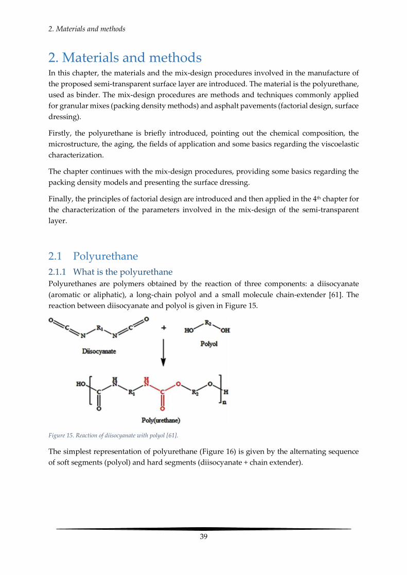
2. Materials and methods
39
2. Materials and methods In this chapter, the materials and the mix-design procedures involved in the manufacture of
the proposed semi-transparent surface layer are introduced. The material is the polyurethane,
used as binder. The mix-design procedures are methods and techniques commonly applied
for granular mixes (packing density methods) and asphalt pavements (factorial design, surface
dressing).
Firstly, the polyurethane is briefly introduced, pointing out the chemical composition, the
microstructure, the aging, the fields of application and some basics regarding the viscoelastic
characterization.
The chapter continues with the mix-design procedures, providing some basics regarding the
packing density models and presenting the surface dressing.
Finally, the principles of factorial design are introduced and then applied in the 4th chapter for
the characterization of the parameters involved in the mix-design of the semi-transparent
layer.
2.1 Polyurethane
2.1.1 What is the polyurethane
Polyurethanes are polymers obtained by the reaction of three components: a diisocyanate
(aromatic or aliphatic), a long-chain polyol and a small molecule chain-extender [61]. The
reaction between diisocyanate and polyol is given in Figure 15.
Figure 15. Reaction of diisocyanate with polyol [61].
The simplest representation of polyurethane (Figure 16) is given by the alternating sequence
of soft segments (polyol) and hard segments (diisocyanate + chain extender).
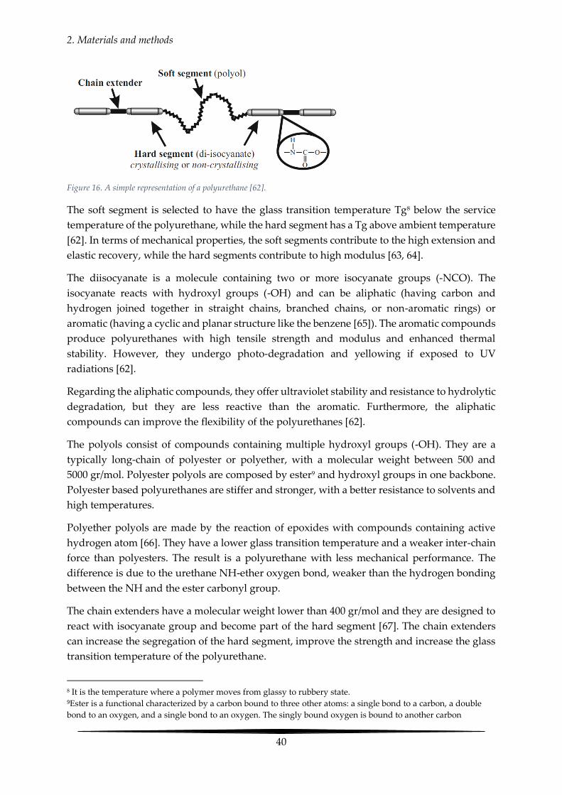
2. Materials and methods
40
Figure 16. A simple representation of a polyurethane [62].
The soft segment is selected to have the glass transition temperature Tg8 below the service
temperature of the polyurethane, while the hard segment has a Tg above ambient temperature
[62]. In terms of mechanical properties, the soft segments contribute to the high extension and
elastic recovery, while the hard segments contribute to high modulus [63, 64].
The diisocyanate is a molecule containing two or more isocyanate groups (-NCO). The
isocyanate reacts with hydroxyl groups (-OH) and can be aliphatic (having carbon and
hydrogen joined together in straight chains, branched chains, or non-aromatic rings) or
aromatic (having a cyclic and planar structure like the benzene [65]). The aromatic compounds
produce polyurethanes with high tensile strength and modulus and enhanced thermal
stability. However, they undergo photo-degradation and yellowing if exposed to UV
radiations [62].
Regarding the aliphatic compounds, they offer ultraviolet stability and resistance to hydrolytic
degradation, but they are less reactive than the aromatic. Furthermore, the aliphatic
compounds can improve the flexibility of the polyurethanes [62].
The polyols consist of compounds containing multiple hydroxyl groups (-OH). They are a
typically long-chain of polyester or polyether, with a molecular weight between 500 and
5000 gr/mol. Polyester polyols are composed by ester9 and hydroxyl groups in one backbone.
Polyester based polyurethanes are stiffer and stronger, with a better resistance to solvents and
high temperatures.
Polyether polyols are made by the reaction of epoxides with compounds containing active
hydrogen atom [66]. They have a lower glass transition temperature and a weaker inter-chain
force than polyesters. The result is a polyurethane with less mechanical performance. The
difference is due to the urethane NH-ether oxygen bond, weaker than the hydrogen bonding
between the NH and the ester carbonyl group.
The chain extenders have a molecular weight lower than 400 gr/mol and they are designed to
react with isocyanate group and become part of the hard segment [67]. The chain extenders
can increase the segregation of the hard segment, improve the strength and increase the glass
transition temperature of the polyurethane.
8 It is the temperature where a polymer moves from glassy to rubbery state. 9Ester is a functional characterized by a carbon bound to three other atoms: a single bond to a carbon, a double
bond to an oxygen, and a single bond to an oxygen. The singly bound oxygen is bound to another carbon

2. Materials and methods
41
2.1.2 Microstructure of a polyurethane
A polymer is defined as amorphous when the molecules are arranged randomly, forming an
unordered structure. If the molecules are tightly packed, forming a regular structure, the
polymer is defined as crystalline. In the case of the polyurethanes, they exhibit both crystalline
and amorphous domains. This type of arrangement is called segmented and it is due to the
polar nature of the hard segments. More in details, the polarity of the hard segments causes a
strong mutual attraction leading to domain formation. This phenomenon, called phase
separation, consists of crystalline or pseudo-crystalline areas located in a soft and flexible
matrix. The rigid segments act as bridges and as filler particles, reinforcing the soft segment
matrix [68].
The phase separation depends on the nature and the size of the soft and hard matrix, the type
of chain extender, of diisocyanate and polyol, the manufacturing process and the reaction
conditions. The degree of phase separation can be controlled by changing the ratio NCO/OH.
For example, the increase in NCO/OH ratio increases the intermolecular attraction of hard to
hard segments due to hydrogen bonding between -NH and –C=O of hard segment, which in
return increases the tensile strength and decreases the elongation [69]. On the contrary, an
excess of polyol (lower NCO/OH ratio) follow the opposite trend [70].
The structure of the polyurethane is also affected by the hydrogen bonds, which occur between
the NH groups and the urethane carbonyl group and, to a lesser extent, between the NH
groups and the ether groups (Figure 17). The hydrogen bonds tie together the polyurethane
chains, forming a “virtually cross-linked structure”. However, the hydrogen bonding is
reversible by means of the heat [68, 71].
Figure 17. Hydrogen bonding between segments in urethane groups [71].
Polyurethanes can be distinguished by thermoset or thermoplastic:
- thermoset polyurethanes have a heavily cross-linked structure and they cannot be
melted after curing. They are characterized by a 3-D rigid structure, due to the covalent
bonds between the linear polymer chains.
- Thermoplastic polyurethanes have a linear structure and they can be deformed
plastically under the effect of the heat [72].
2. Materials and methods
42
2.1.3 Definition of curing
Curing is the crosslinking process of the molecules in a polymer. The crosslinking is
accomplished by catalysts or curing agents able to control the time and temperature to
complete the reaction [73].
The crosslinking affects the physical properties of the polymer. For instance, the increase of
crosslinks can make the polymer more rigid, because of the strong covalent bonds.
Once the polymerization is triggered, the crosslinking starts and the molecules become larger
and less mobile. During the network formation (gelation), the polymer consists of two phases:
the phase of the gel fraction and the unreacted gel. The gel fraction has a glass transition
temperature higher than the unreacted fraction. With the continuation of the reaction, the glass
transition temperature increases until reaching a maximum, which represents the glass
transition temperature of the polymer fully cured [74].
The curing depends on the mobility and reactivity of the reactants and on the surrounding
temperature. The curing could also continue for a long time if unreacted groups remain in the
polymer. In addition, physical aging could occur, causing residual stresses.
2.1.4 Introduction to polymer aging mechanisms
The term aging refers to properties changes of a polymer over a period of time. The changes
may involve engineering properties such as stiffness and toughness linked to chemical
characteristics such as reactivity towards aggressive chemicals. Aging can be distinguished by
physical, thermal and weathering [74, 75].
Physical ageing is very common in thermoplastic polyurethanes and it occurs when the
material moves from high temperature during the shape operations to low temperature. Once
below the glass transition temperature, the rate of molecular relaxation is too slow to maintain
the material in a thermodynamic equilibrium. As a result, the polymer undergoes volumetric
relaxation, gradually increasing its density during an extended ageing period.
Thermal aging refers to the chemical and physical degradation processes that occur at high
temperatures. Increased temperature accelerates the oxidation and the mechanical creep. In
particular, the oxidation could trigger other chemical reactions that may occur very slowly at
room temperature.
Thermal degradation is also affected by the aging temperature. In general, the rate of aging is
increased by a factor of 2ΔT/10, where ΔT is the increase of temperature [76].
Finally the weathering, named also ‘’natural aging”, is the exposition of polymers to
environmental agents such as solar radiation, water, pollutants and temperature changes.
Weathering is mostly due to the photodegradation, which is the degradation of a molecule
caused by the absorption of photons, because of the exposition to the sunlight radiations

2. Materials and methods
43
(Figure 18). There are three steps of photodegradation: initiation, propagation and
termination.
The initiation can start with the reaction between free radicals (atom or molecule with
unpaired valence electron) and oxygen, forming peroxy radicals (ROO).
In the propagation, the peroxy radicals are able to abstract hydrogens from the polymer chains
to form hydroperoxide (ROOH), which is the most important initiator of photodegradation.
In termination, hydroperoxydes split again in two free radicals (RO· + ·OH), which can
recombine or continue to attach the polymer chain. In the case of recombination, typical of
polyethylene or rubber, the polymer becomes more brittle and shows cracking. In the case of
chain scissions, typical of natural rubber, it leads to softening and to reduction of mechanical
properties of the polymer [77, 78].
Figure 18. Photodegradation cycle for polymers [78].
2.1.5 Applications of polyurethanes
The polyurethane is a versatile material and it can be synthesized for specific applications in
constructions, automotive, textile and in several other industries. The Table 5 lists the main
types of polyurethanes, pointing out properties, chemistry and applications:
Type of
polyurethane Properties Chemistry Applications
Thermoplastic
Modulable flexibility,
mechanical strength and
elasticity, good abrasion
resistance, and
transparency [79]
It is a multi-phase block
copolymer obtained
combining together three
components: i) A polyol or
long-chain diol, ii) a chain
extender or short-chain diol,
iii) a diisocyanate [80]
Outer cases of
electronic devices,
automotive
instrument panels,
medical devices,
sporting goods [81]
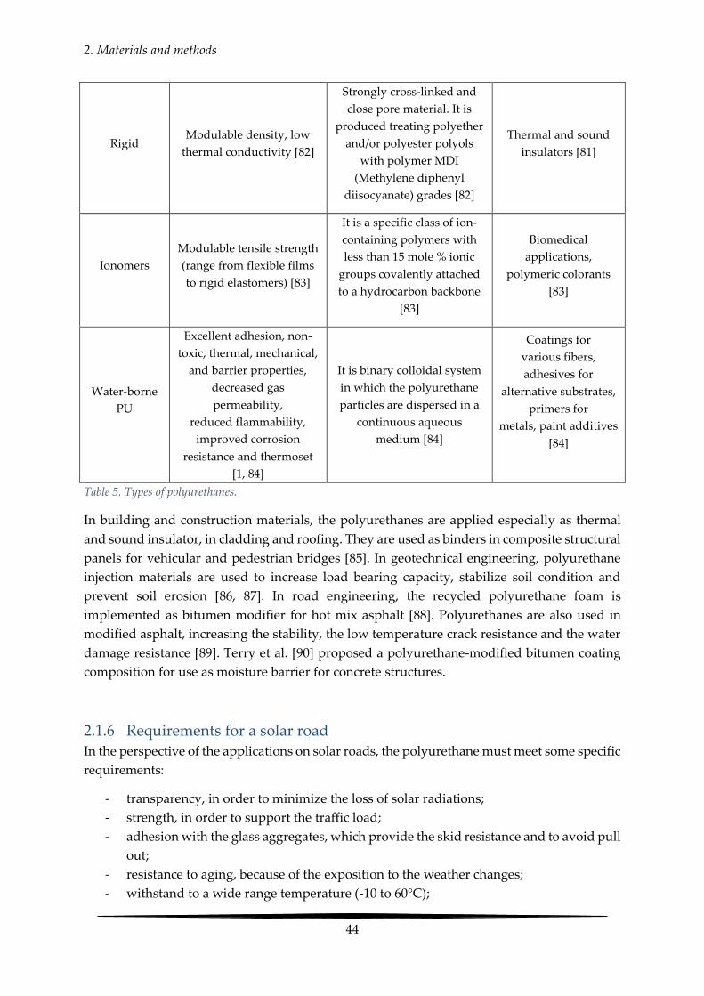
2. Materials and methods
44
Rigid Modulable density, low
thermal conductivity [82]
Strongly cross-linked and
close pore material. It is
produced treating polyether
and/or polyester polyols
with polymer MDI
(Methylene diphenyl
diisocyanate) grades [82]
Thermal and sound
insulators [81]
Ionomers
Modulable tensile strength
(range from flexible films
to rigid elastomers) [83]
It is a specific class of ion-
containing polymers with
less than 15 mole % ionic
groups covalently attached
to a hydrocarbon backbone
[83]
Biomedical
applications,
polymeric colorants
[83]
Water-borne
PU
Excellent adhesion, non-
toxic, thermal, mechanical,
and barrier properties,
decreased gas
permeability,
reduced flammability,
improved corrosion
resistance and thermoset
[1, 84]
It is binary colloidal system
in which the polyurethane
particles are dispersed in a
continuous aqueous
medium [84]
Coatings for
various fibers,
adhesives for
alternative substrates,
primers for
metals, paint additives
[84]
Table 5. Types of polyurethanes.
In building and construction materials, the polyurethanes are applied especially as thermal
and sound insulator, in cladding and roofing. They are used as binders in composite structural
panels for vehicular and pedestrian bridges [85]. In geotechnical engineering, polyurethane
injection materials are used to increase load bearing capacity, stabilize soil condition and
prevent soil erosion [86, 87]. In road engineering, the recycled polyurethane foam is
implemented as bitumen modifier for hot mix asphalt [88]. Polyurethanes are also used in
modified asphalt, increasing the stability, the low temperature crack resistance and the water
damage resistance [89]. Terry et al. [90] proposed a polyurethane-modified bitumen coating
composition for use as moisture barrier for concrete structures.
2.1.6 Requirements for a solar road
In the perspective of the applications on solar roads, the polyurethane must meet some specific
requirements:
- transparency, in order to minimize the loss of solar radiations;
- strength, in order to support the traffic load;
- adhesion with the glass aggregates, which provide the skid resistance and to avoid pull
out;
- resistance to aging, because of the exposition to the weather changes;
- withstand to a wide range temperature (-10 to 60°C);

2. Materials and methods
45
- workability
Among all the types of polyurethane, the thermoset polyurethane seems to be the best
candidate because it can’t be melt by means of temperature; it has high modulus, excellent
adhesion, good resistance to aging and good transparency.
2.2 Mix design methods
2.2.1 Particle packing degree The mechanical performance of granular mixes such as asphalt and concrete is strongly
affected by the particle packing degree. The optimization of the selected aggregate materials
allows to reduce the porosity and to minimize the amount of binder required to the air voids.
In the light of this, the study of the packing density could be useful for the mix-design of the
semi-transparent layer.
Particle packing models seek to select proper sizes and proportion of particles to fill larger
voids in the mix of concrete or asphalt. The packing density α is defined as the ratio between
the solid volume and the total volume. The remaining void is the porosity of the medium,
given by 1-α.
Particle packing models can be categorized as [91]:
- Discrete models: mix containing two or more discrete size classes of particles and
each class of particles is packed to its maximum density in the available volume;
- Continuous models: mix containing all the possible sizes.
2.2.1.1 Discrete models
Furnas was one of the first authors to work on the problem of the particle packing and he
proposed a discrete model valid for two monosized aggregate groups without interaction
between the particles [91].
The partial volume of each class is called ϕi and it represents the volume occupied by the class
i in a unit volume. While the relative volume of each class is called ri. In general [92]:
∑ ri = 1ni=1 ; and ri = φi/∑ φi
ni=1 4
For two size classes, two cases are distinguishable:
- Case 1: the volume fraction of the big particles is larger than the volume fraction of the
small particles (r1 ˃˃ r2). In this case, called “coarse grain dominant”, the small
particles are added in a container in order to fill the voids between the large particles.
Consequently, the packing density αt is given by the volume of the big particles plus
the volume of small particles, in a unit volume:

2. Materials and methods
46
αt = φ1 + φ2 = α1 + φ2 → αt =α1
1 − r2=α1r1 5
- Case 2: the volume fraction of the small particles is larger than the volume fraction of
the large particles (r2˃˃r1). In this case, called “fine grain dominant”, few large
particles are added in a container already filled with small particles. The total packing
density is obtained by the volume of the big particles plus the remaining volume (1-ϕ1)
filled with the small particles at their maximum packing density:
αt = φ1 + φ2 = φ1 + α2(1 − φ1) → αt =1
r1 + (r2α2)
6
If r1≈r2, interaction effects are not negligible and they cause the increase of voids in the
mixture.
There are two types of interaction effects [93]:
- The wall effect, when an isolated coarse aggregate is in a matrix of small particles (the
result is an increased voids in the region of direct contact between the particles);
- The loosening effect, when a fine particle is in a matrix of coarse particles, but its
dimension is too large to fit properly the voids between the large aggregates. The
interaction causes a reduction of the packing density.
Figure 19. Schematic representation of the wall effect and the loosening effect [93].
Another binary model was proposed by Aim and Toff [94]. The value of packing density φ is
given by:
ϕ =
{
(1 − ε2)
(1 − φ1), φ1 ≤ φ1 ∗
(1 − ε2)
[φ1 + (1 − φ1) (1 +0.9d1d2
) (1 − ε2)], φ1 > φ1 ∗
7

2. Materials and methods
47
φ1 ∗=1 − (1 + 0.9d1/d2)(1 − ε2)
2 − (1 + 0.9d1/d2)(1 − ε2) 8
Where:
- ε2 = void ratio of large-grained material;
- d1 = average diameter of small grains;
- d2 = average diameter of large grains;
- ϕ1 = volume fraction of small-grained materials.
When ϕ1 = ϕ1*, the equation of packing density is:
ϕ ∗= (1 − ε2)[2 − (1 + 0.9d1/d2)(1 − ε2)] 9
Toufar [91] developed a model for a mixture having a diameter ratio 0.22 ˂ d1/d2 ˂ 1.0. The
concept is that the smaller particles (d1/d2 ˃ 0.22) are too large to be situated in the voids
between the larger particles d2. The possible results are: i) a mixture mostly composed of large
particles and ii) a mixture composed of small particles, with some large aggregate in the
matrix. In the case of multi-component system, the matrix is given by the contribution of
different binary mixtures.
Moved from the Toufar studies, Golterman [95] proposed a model validated by comparing
around 800 test results from multiple sources. The packing density formula is:
φ =1
[y1φ1+y2φ2
− y2 (1φ2
− 1)kdks]
10
Where:
- y1/ϕ1 = bulk volume of the fine particles;
- y2/ϕ2 = bulk volume of the coarse particles;
- 𝑦2 (1
𝜑2− 1) = void volume between the coarse particles:
- 𝑘𝑑 =𝑑2−𝑑1
𝑑1+𝑑2 factor depending on the diameter ratio of the particles;
While ks is a statistical factor depending on the ratio between the bulk volume of the fine
particles and the void volume between the coarse particles. In particular:
ks = 1 −1 + 4x
(1 + x)4
11
x =(y1y2) (
φ2φ1)
(1 − φ2) 12
Tests demonstrated that, adding a small quantity of fine particles, the packing density didn’t
increase. The reason is because the fine particles are confined in the voids between the coarse
particles. This observation was introduced in the model using the follow expression of ks:

2. Materials and methods
48
ks = k0 (x
x0) for x˂x0 13
Where:
- x0 = 0.4753;
- k0 = 0.3881
If x ≥ x0, the value of ks is given by the equation:
ks = k0 (x
x0) for x˂x0 14
All those models, although efficient, remained limited by their limited number of size classes
taken into account. The need for generalized models led to the development of the one
described next.
2.2.1.2 Continuous models
In the continuous models, all possible sizes of aggregates are present in the medium. Fuller
and Thomson [91] proposed a simple equation to maximize the packing density:
CPFT = (d
D)n
∙ 100 15
Where:
- d is the particle size;
- D is the maximum particle size;
- CPFT is the cumulative volume percent finer than d;
- n is equal to 0.45.
Andersen [91] developed an equation similar to the (15), assuming that the fine particles are
infinite small. The formula is:
CPFT = (d
D)q
∙ 100 16
Where q ranges between 0.21 and 0.37.
In 1994, Funk and Dinger [91] modified the Andersen model, removing the hypothesis that
the fine particles are infinite small and introduce the term d0, representing the minimum
particle size distribution. The new equation becomes:
CPFT = [(d − d0)
(D − d0)]
q
∙ 100 17
2.2.1.3 De Larrard Model
De Larrard Model [93], also called Compressive Packing Model (CPM), is able to predict the
packing density of a polydisperse grain mixture taking into account: i) the size of the grains;
ii) the shape of the grains and iii) the method of processing the packing.

2. Materials and methods
49
Firstly, De Larrard developed a model to calculate the virtual packing density, which
represents the maximum packing density achieved if each aggregate was placed individually.
The data input were the grain size distribution and the residual packing density βi.
The virtual packing density didn’t take into account the packing process. For this reason, the
model was improved by introducing a novel parameter called compaction index K.
Mathematically, the compaction index is given by:
K =∑Ki =∑
ϕiϕi∗
1 −ϕiϕi∗
n
i=1
n
i=1
18
Where:
- ɸi is the actual solid volume of the class i;
- ɸi* is the maximum volume that the particles i may occupy, considering the presence
of the other particles.
The compaction index increases according to the energy of compaction, in particular it ranges
from 4.1 to 9 (loose packing and dense compressed and vibrated packing, respectively).
Theoretically, K can tend to infinite, which corresponds to the virtual packing density.
Finally, the model was generalized introducing a boundary condition due to the presence of
the container. The idea is that the voids increase because of the perturbation due to the
container. In particular, the increase of voids is proportional to the contact surface of the
container and to the size of the aggregates.
Figure 20. Wall effect due to the container [93].
Ben-Aïm [96] speculated the existence of a perturbed volume Vp within a distance of d/2 from
the surface of the container. In this volume the mean packing density is given by kwα, where
kw is a coefficient less than 1, while α is the packing density in the non-perturbed area of the
container. The mean packing density for the whole container is given by:
α̅ = (1 − Vp)α + Vpkwα = [1 − (1 − kw)Vp]α 19

2. Materials and methods
50
2.2.2 The surface dressing The surface dressing is a low-cost, highly effective and simple road surface treatment. It is able
to seal the fine cracks in the pavement, prevent water infiltration in the base and subbase,
improve the skid-resistance of the surface and extend the expected life of the infrastructure
[97].
The surface dressing consists of a thin film of binder, which is spread on the road surface and
covered with a layer of stone chippings. In general, it can be corrective or preventive. The
corrective is performed to restore distressed road sections, while the preventive is performed
to prevent (or reduce) the damage development.
The time between two surface dressing applications can vary from less than one year to more
than eight years. For a traffic flow less than 500 vehicles per day, its performance can be
significantly higher. The performance of the surface dressing is also affected by other
parameters such as: size and shape of the aggregates, conditions of the pre-treated road, binder
application rates, pavement temperature at the time of treatment, speed of the traffic in the
period immediately following the treatment and level of supervision of the application of a
treatment [98].
The success of the surface dressing treatment starts from a formal analysis of the following
characteristics [99]:
- Evaluate the surface texture, in particular the nominal aggregate size, which affects the
skid resistance and the noise level of the road;
- Evaluate traffic conditions, in order to select the best surface dressing treatment;
- Evaluate climatic and seasonal characteristics; it was observed that surface dressing
performed better in the dry/no-freeze zones.
- Evaluate and select the type of chip seal; the construction procedure, the number of
courses sealed, and variations in aggregate nominal size make the difference in the
type of treatment
- Evaluate the aggregate selection; the selection of the aggregate size determines the
thickness of surface dressing. The increase of the aggregates size makes the texture
rougher, increasing the level of noise. According to the Montana DOT [102] the best
aggregate for the surface dressing should have a maximum particle size of 9.5 mm,
cubical or pyramidal shape, an absence of fine particles (less than 2% passing to the
sieve No. 200) and abrasion not exceeding the 30%.
- Determine the binder application rate; an approach is to achieve a 50% aggregates
immersion after rolling and finishing the embedment to the vehicles. Alternatively, the
aggregates immersion could be up to 70%. In this case, the pull out of aggregates is
reduced, but the road could be prone to bleeding
- Determine how many hours per day are available for construction operations.
This approach is based on the assumption that surface dressing requires the use of uniformly
graded aggregates spread in a one stone thick layer in a uniform manner.

2. Materials and methods
51
There are other specific methods for the mix-design of the surface dressing. Among these, one
of the most advanced is the Road Note 39, based on the extensive use of decision trees. Primary
inputs of the method are the traffic level, road hardness, surface conditions, geometry of the
site, while secondary inputs are the skid resistance requirements and the weather conditions.
The method continues with the following 5 steps: i) selection of the type of surface dressing;
ii) selection of the type of binder; iii) selection of the aggregates (20, 14, 10, 6 or 3 mm nominal
size); iv) binder spread rate (depending on the size and the shape of the aggregates, their
nature and the level of immersion into the binder); v) rate of the aggregate spread.
The selection of the surface dressing treatment depends on traffic level and construction
season. Regarding the aggregates, the choice is based on the skid resistance requirements and
the hardness of the existing surface. Finally, the binder and the aggregate spread rates depend
on the size, the shape and the nature of the aggregates.
Other details, based on the chosen surface dressing treatment, are given by the French
specifications. For example, in the case of a single layer of surface dressing having aggregates
dimension between 2 and 4 mm, the aggregate spread rate is 5 l/m2, while binder spread rate
is between 0.8 and 1 kg/m2 [103].
2.2.3 The factorial design The factorial design is a method able to study the influence of each experimental variable and
their interaction on the response of the investigated system.
In the field of road engineering, the factorial design method has been applied on many
occasions for example to investigate the resilient modulus of bituminous paving mixes [104],
or to analyze the effect of recycled coarse aggregates percentage and bitumen content
percentage on various parameters such as stability, flow, air void, void mineral aggregate,
void filled with bitumen, and bulk density [105]. Wang et al studied the effects of basalt fiber
content, length, and asphalt-aggregate ratio on the volumetric and strength properties of
styrene–butadiene–styrene (SBS)-modified asphalt mixture [106]. A two-level factorial design
was developed to evaluate the effects of the test temperature and of a surfactant warm additive
on the visco-elastic behavior of bitumen [107]. Kabagire and Yahia applied the full-factorial
design on pervious concrete, in order to study the effect of three mixture parameters (paste
volume- to-inter-particles void ratio, water-to-cement ratio, and dosage of water reducing
agent) on permeability, effective porosity, unit weight, and compressive strength [108].
Zou et al evaluated the effect of asphalt mixture type, temperature, loading frequency and tire-
pavement contact pressure on the wheel tracking test [109].
Based on the literature, the factorial design seems to be a good method to better-understand
the effects of a high number of variables on the outcome of the investigated system, especially
when the modeling of the system is complex.
2. Materials and methods
52
2.2.3.1 Basics of factorial design
The factorial design is a multipurpose tool that can be used in various situations for
identification of important input factors (input variable) and how they are related to the
outputs [110]. If the influence of a certain number of h variables is investigated, the factorial
design will consist of 2h experiments.
Each experiment provides a system’s response, according to the variable combinations. The
goal is to describe the response of the system fitting a multiple regression model given by:
y = a0 +∑aixi +∑aijxixj +⋯+∑aiixi2 + aij…zxixj…xz + e 20
Considering only the second order interactions, the Eq. 20 becomes:
y = a0 +∑aixi +∑aijxixj + e 21
The factorial design can be defined as a system of n equations (each equation is given by an
experiment) and p variables [111], which can be written in matrix format as:
y̅ = X̿a̅ + e̅ 22
Where:
- �̅� is the vector with the outcome of the experiments;
- �̿� is the model matrix, depending on the interactions between the variables;
- �̅� is the vector with the coefficient of the regression model;
- �̅� is the error.
In most investigations it is reasonable to assume the influence of the third order or higher is
negligible. It means that it is possible to reduce the number of experiments, changing from 2h
to 2h-p experiments. This method is called fraction factorial design, where p is the size of the
fraction.
On reducing the number of experiments and consequently of the equations, the system (22) is
no longer solvable (n number of equations <p unknown coefficients). The idea is to cofound
some effects, defining some equivalences between the variables and consequently reduce the
unknown coefficients [112].
2.3 Conclusions The aim of this chapter was to introduce and assist the reader for a better-understanding of
the manuscript. The materials and the methods/techniques presented so far will be applied in
the following chapters for the mix-design of the semi-transparent layer.
Based on the literature review, the polyurethane seems to be a good candidate as binder in
solar roads. In particular, the thermoset polyurethane guarantees high stiffness, excellent
adhesion, good aging resistance and good transparency.

2. Materials and methods
53
The mix-design of the semi-transparent layer using the polyurethane has not been investigated
so far. At this scope, the author identified the packing density, the surface dressing and the
factorial design as suitable methods/techniques for its mix-design.
The packing density methods are useful to reduce the air voids in the mix and optimize the
use of binder. Instead, the surface dressing is a new way of understanding of the semi-
transparent layer. The procedure consists in spreading a thin film of polyurethane and cover
it with the glass aggregates, alike the bitumen covered by stone chippings.
Another approach applied for this thesis is to investigate the effect of each parameter involved
in the mix design (binder content, particle size distribution and thickness) by means of the
fraction factorial design. It is encouraging to know that other authors have successfully applied
this method to study and optimize the mechanical performance of asphalt mixtures.


3. Polymerization and viscoelastic behavior of the polyurethane according to curing temperature
55
3. Polymerization and viscoelastic behavior of the
polyurethane according to curing temperature The polymerization and the viscoelastic behavior of the polyurethane is strictly dependent on
the temperature. Furthermore, there are no specifications or guidelines for the using of this
material as binder in solar road. For this reason, the 3rd chapter focuses on the understanding
of the polyurethane behavior. Four thermoset polyurethanes are characterized in terms of
curing kinetic and viscoelastic behavior by means of the Dynamic Shear Rheometer (DSR) and
the Dynamic Mechanical Analysis (DMA). The results are modeled according to the Arrhenius
law and generalized Maxwell model. The objectives are to:
i) understand the suitability of the polyurethane as binder,
ii) understand how the chemical structure and composition of the polyurethane affects
its viscoelastic behavior,
iii) define the best conditions for outdoors implementation, paying attention to the
influence of the temperature on the curing time and on the mechanical performance.
3.1 Presentation of the materials: the thermoset polyurethanes The materials used for this research are four thermoset polyurethanes, expressly
manufactured by RPM Belgium Vandex Company according to the requirements defined in
the paragraph “Requirements for a solar road”.
Each polyurethane is obtained by combining two components: part α, containing the polyols
and part β, containing the diisocyanates. For the experimentations, part α and part β are mixed
together manually for 2 minutes, at room temperature, according to the mass fraction
recommended by the company.
The main properties of the products are summarized in Table 6.
Ref. Part
Boiling
point
[°C]
Flash
point
[°C]
Viscosity
[Pa s]
Density
[gr/cm3]
Mass
fraction
[%]
A Α 170 220 3 (20 °C) 1 50
Β NA 158 1.2 (20 °C) 1.2 50
B Α 170 200 0.7 (20 °C) 1 47.5
Β 285 203 1 (20 °C) 1.15 52.5
C Α 200 70 0.6 (20 °C) 1.3 58.7
Β 200 200 1 (20 °C) 1.13 41.3
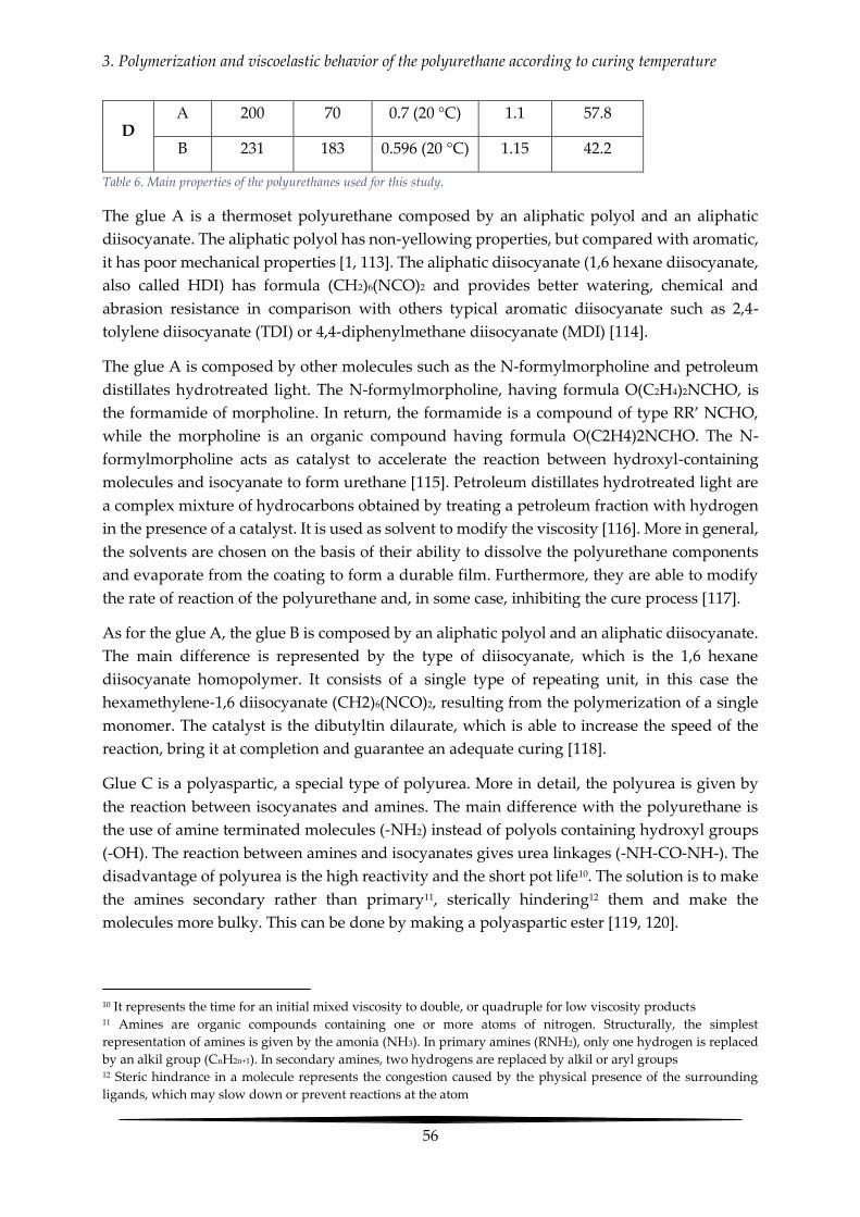
3. Polymerization and viscoelastic behavior of the polyurethane according to curing temperature
56
D Α 200 70 0.7 (20 °C) 1.1 57.8
Β 231 183 0.596 (20 °C) 1.15 42.2
Table 6. Main properties of the polyurethanes used for this study.
The glue A is a thermoset polyurethane composed by an aliphatic polyol and an aliphatic
diisocyanate. The aliphatic polyol has non-yellowing properties, but compared with aromatic,
it has poor mechanical properties [1, 113]. The aliphatic diisocyanate (1,6 hexane diisocyanate,
also called HDI) has formula (CH2)6(NCO)2 and provides better watering, chemical and
abrasion resistance in comparison with others typical aromatic diisocyanate such as 2,4-
tolylene diisocyanate (TDI) or 4,4-diphenylmethane diisocyanate (MDI) [114].
The glue A is composed by other molecules such as the N-formylmorpholine and petroleum
distillates hydrotreated light. The N-formylmorpholine, having formula O(C2H4)2NCHO, is
the formamide of morpholine. In return, the formamide is a compound of type RR’ NCHO,
while the morpholine is an organic compound having formula O(C2H4)2NCHO. The N-
formylmorpholine acts as catalyst to accelerate the reaction between hydroxyl-containing
molecules and isocyanate to form urethane [115]. Petroleum distillates hydrotreated light are
a complex mixture of hydrocarbons obtained by treating a petroleum fraction with hydrogen
in the presence of a catalyst. It is used as solvent to modify the viscosity [116]. More in general,
the solvents are chosen on the basis of their ability to dissolve the polyurethane components
and evaporate from the coating to form a durable film. Furthermore, they are able to modify
the rate of reaction of the polyurethane and, in some case, inhibiting the cure process [117].
As for the glue A, the glue B is composed by an aliphatic polyol and an aliphatic diisocyanate.
The main difference is represented by the type of diisocyanate, which is the 1,6 hexane
diisocyanate homopolymer. It consists of a single type of repeating unit, in this case the
hexamethylene-1,6 diisocyanate (CH2)6(NCO)2, resulting from the polymerization of a single
monomer. The catalyst is the dibutyltin dilaurate, which is able to increase the speed of the
reaction, bring it at completion and guarantee an adequate curing [118].
Glue C is a polyaspartic, a special type of polyurea. More in detail, the polyurea is given by
the reaction between isocyanates and amines. The main difference with the polyurethane is
the use of amine terminated molecules (-NH2) instead of polyols containing hydroxyl groups
(-OH). The reaction between amines and isocyanates gives urea linkages (-NH-CO-NH-). The
disadvantage of polyurea is the high reactivity and the short pot life10. The solution is to make
the amines secondary rather than primary11, sterically hindering12 them and make the
molecules more bulky. This can be done by making a polyaspartic ester [119, 120].
10 It represents the time for an initial mixed viscosity to double, or quadruple for low viscosity products 11 Amines are organic compounds containing one or more atoms of nitrogen. Structurally, the simplest
representation of amines is given by the amonia (NH3). In primary amines (RNH2), only one hydrogen is replaced
by an alkil group (CnH2n+1). In secondary amines, two hydrogens are replaced by alkil or aryl groups 12 Steric hindrance in a molecule represents the congestion caused by the physical presence of the surrounding
ligands, which may slow down or prevent reactions at the atom
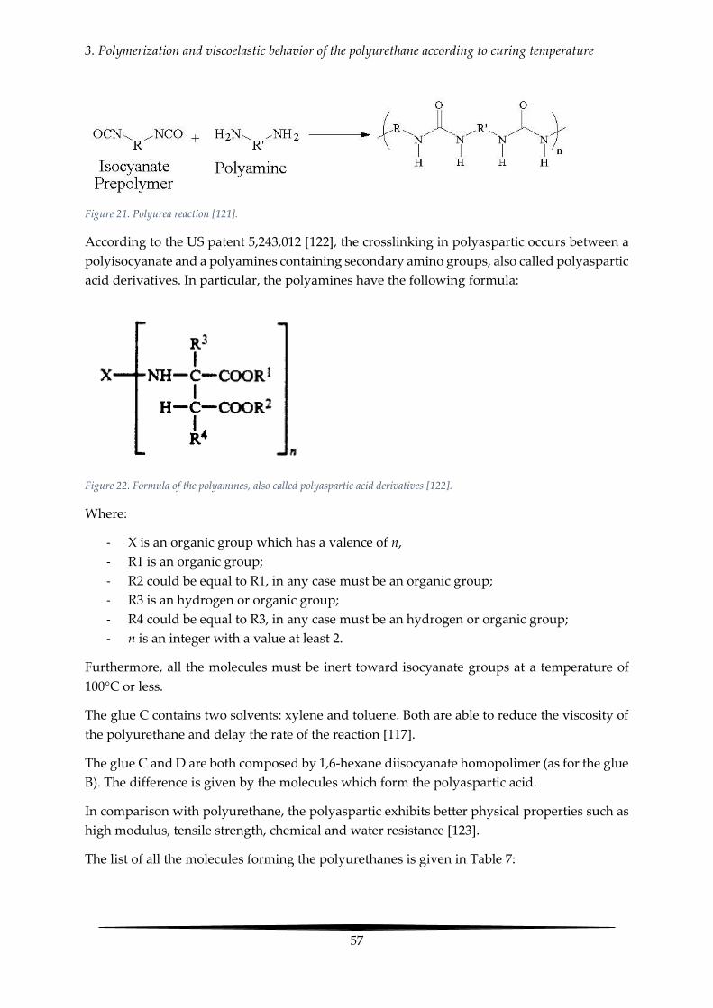
3. Polymerization and viscoelastic behavior of the polyurethane according to curing temperature
57
Figure 21. Polyurea reaction [121].
According to the US patent 5,243,012 [122], the crosslinking in polyaspartic occurs between a
polyisocyanate and a polyamines containing secondary amino groups, also called polyaspartic
acid derivatives. In particular, the polyamines have the following formula:
Figure 22. Formula of the polyamines, also called polyaspartic acid derivatives [122].
Where:
- X is an organic group which has a valence of n,
- R1 is an organic group;
- R2 could be equal to R1, in any case must be an organic group;
- R3 is an hydrogen or organic group;
- R4 could be equal to R3, in any case must be an hydrogen or organic group;
- n is an integer with a value at least 2.
Furthermore, all the molecules must be inert toward isocyanate groups at a temperature of
100°C or less.
The glue C contains two solvents: xylene and toluene. Both are able to reduce the viscosity of
the polyurethane and delay the rate of the reaction [117].
The glue C and D are both composed by 1,6-hexane diisocyanate homopolimer (as for the glue
B). The difference is given by the molecules which form the polyaspartic acid.
In comparison with polyurethane, the polyaspartic exhibits better physical properties such as
high modulus, tensile strength, chemical and water resistance [123].
The list of all the molecules forming the polyurethanes is given in Table 7:

3. Polymerization and viscoelastic behavior of the polyurethane according to curing temperature
58
Glue A
Hermapur 2700 UV
part α
Aliphatic polyols (contain hydrocarbon) +
Distillates (petroleum), hydrotreated light (hydrocarbon) +
4-Morpholinecarboxaldehyde (organic compound)
Hermapur 2700 UV
part β Hexane – 1,6 – diisocyanate
Glue B
Hermapur 2700 UV
improved version
part α
1,6-Hexane-diyl-bis-carbamate bis(2-(2-(1-ethylpentyl)-3-ox
azolidinyl)ethyle) +
Aliphatic polyol +
Alkylammonium salt +
Dibutyltin dilaurate (catalyst)
Solvent naphtha, light aromatic
Hermapur 2700 UV
improved version
part β
Hexamethylene-1,6-diisocyanate homopolymer (HMDI)
Glue C
Hermapur 3002
part α
Bis(4-(1,2-bis(éthoxycarbonyl)-éthylamino)-3-méthyl-
cyclohexyl)-méthane +
Aspartic acid, n,n'-(methylenedi-4,1-c yclohexanediyl)bis-
,1,1',4,4'-tetraethyl ester +
Ester of asparagine acid +
Xylene +
Ethylbenzene +
Toluene
Hermapur 3002
part β Hexane – 1,6 – diisocyanate homopolymer
Glue D
Hermapur 30xx
Part α
Bis(4-(1,2-bis(éthoxycarbonyl)-éthylamino)-3-méthyl-cyclo
hexyl)-méthane +
Aspartic acid, n,n'-(methylenedi-4,1-c yclohexanediyl)bis-,
1,1',4,4'-tetraethyl ester +
Naphtha (petroleum), heavy alkylate +

3. Polymerization and viscoelastic behavior of the polyurethane according to curing temperature
59
Polyalkalene HMTS +
1-Methoxy-2-propyl acetate +
2-methoxypropyl acetate
Hermapur 30xx
Part β
Hexane – 1,6 – diisocyanate homopolymer
1,6-hexane diisocyanate
Table 7. Chemical composition of the polyurethanes.
3.2 Viscoelastic characterization of the polyurethane
3.2.1 Basics of viscoelastic characterization
The viscoelastic characterization of the polyurethanes can be performed by means of the
Dynamic Shear Rheometer (DSR) and the Dynamic Mechanical Analysis (DMA). Both devices
enable the measurements of the complex modulus according to linear viscoelasticity theory
framework. The complex modulus (G* or E*) is measured in sinusoidal mode of loading in the
small strain domain [124, 125]. It is defined as the relationship between complex strain and the
complex stress (Eq. 23):
τ∗ = G∗γ∗ 23
or:
σ∗ = E∗ε∗ 24
The complex modulus is given by two components (Eq. 24 and Eq. 25):
G∗ = G′ + iG′′ = |G∗|exp(iδ) in shear mode loading 25
E∗ = E′ + iE′′ = |E∗|exp(iδ) in tension-compression mode of loading 26
Where:
- G* is the complex shear modulus;
- τ* is the complex shear stress;
- γ* is the complex shear strain;
- E* is the complex tension-compression modulus;
- σ* is the complex stress
- ε* is the complex strain;
- G’ (or E’) is the elastic modulus, which represents the ability of the material to store
energy;
- G’’ (or E’’) is the viscous modulus, which represent the ability of the material to
dissipate energy;
- |G*|(or |E*|) is the magnitude of the complex modulus;

3. Polymerization and viscoelastic behavior of the polyurethane according to curing temperature
60
- δ is the ratio of the viscous and the elastic components of the complex modulus (Eq.
26):
δ = tan−1 (G′′
G′) 27
The DSR is used to measure the viscoelastic behavior of asphalt binders, polymers or glues at
different temperatures and frequencies. The basic DSR is composed of two circular plates: the
lower plate is fixed while the upper plate oscillates back and forth across the sample (Figure
23) for a set frequency in order to create a shearing action [126].
Figure 23. A simple representation of a DSR in oscillation mode [127].
The DSR measures the complex shear modulus (G*) and the phase angle (δ). The complex
shear modulus (G*) can be considered as the sample’s total stress response to deformation
when repeatedly sheared, while the phase angle (δ), is the lag between the applied shear stress
and the resulting shear strain. The larger the phase angle (δ), the more viscous the material.
Phase angle limiting values are:
- Purely elastic material: δ = 0°
- Purely viscous material: δ = 90°
Considering now the applied shear stress, it can be decomposed vectorially in two
components: one in phase with strain and one 90° out of phase. Dividing them by the strain,
the result is the modulus in phase (real part) and out-of-phase (imaginary).
The DMA (Figure 24) supplies an oscillatory force, causing a sinusoidal stress, applied to a
sample. The response of the material is a sinusoidal strain. Unlike the DSR, the oscillatory force
isn’t a shear force, but a tension-compression force. In other terms, the DMA is able to measure
directly the complex modulus E* (the DSR measures the shear complex modulus G*) [128].

3. Polymerization and viscoelastic behavior of the polyurethane according to curing temperature
61
Figure 24. Schematic representation of the DMA performed on a cylinder of bitumen [129].
The modulus is dependent of the temperature. For example, if a polymer is heated so that it
exceeds the glass transition temperature, the modulus will drop dramatically.
One advantage of the DMA is the possibility to sweep across temperature and/or frequency
ranges. It means that applying 1 Hz, the modulus can be recorded every second, while varying
the temperature at some rate, for example 10 °C/min. Based on the same approach, it is possible
to scan a wide range of frequency from 0.01 to 100 Hz.
The modulus measured by the DMA is the complex tension-compression modulus E*,
composed by the real part (elastic modulus E’) and the imaginary part (E’’), which represents
the ability of the material to store energy and dissipate energy, respectively (Eq. 26).
3.2.2 Experimental plan
For the characterization of the polyurethanes, an experimental campaign (Figure 25) was
conducted performing the tests by means of the Dynamic Shear Rheometer (DSR) and the
Dynamic Mechanical Analysis (DMA).
The DSR was used here to measure the complex shear modulus (G*) during the polymerization
process of the polyurethanes at the frequency of 1 Hz and at constant temperature. The goal
was to determine the curing kinetic of the different binders at 50, 30 and 10 °C.
The DMA was performed at achieved polymerization, with solid sample, and it provided the
complex modulus in tension compression for various frequencies and temperatures. The goal
was to determine the curing temperature effect on the mechanical properties of the different
glues. Finally, the results were compared with the bitumen 35-50, widely used in the asphalt
concrete.
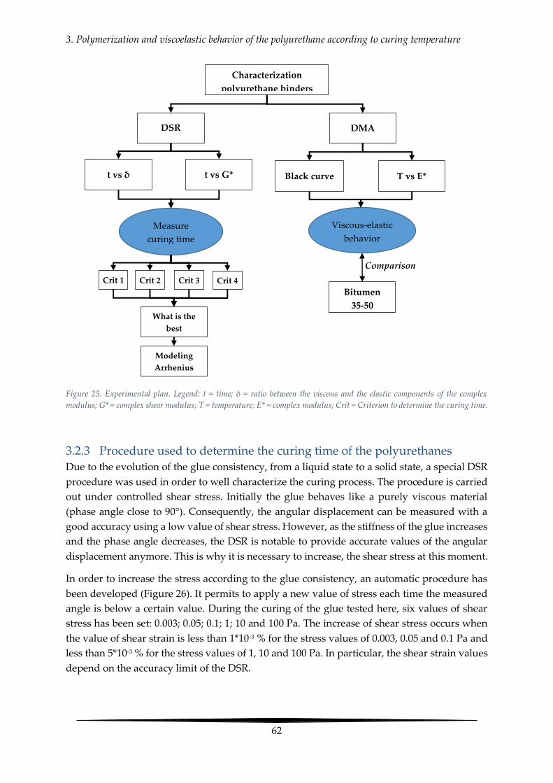
3. Polymerization and viscoelastic behavior of the polyurethane according to curing temperature
62
Figure 25. Experimental plan. Legend: t = time; δ = ratio between the viscous and the elastic components of the complex
modulus; G* = complex shear modulus; T = temperature; E* = complex modulus; Crit = Criterion to determine the curing time.
3.2.3 Procedure used to determine the curing time of the polyurethanes
Due to the evolution of the glue consistency, from a liquid state to a solid state, a special DSR
procedure was used in order to well characterize the curing process. The procedure is carried
out under controlled shear stress. Initially the glue behaves like a purely viscous material
(phase angle close to 90°). Consequently, the angular displacement can be measured with a
good accuracy using a low value of shear stress. However, as the stiffness of the glue increases
and the phase angle decreases, the DSR is notable to provide accurate values of the angular
displacement anymore. This is why it is necessary to increase, the shear stress at this moment.
In order to increase the stress according to the glue consistency, an automatic procedure has
been developed (Figure 26). It permits to apply a new value of stress each time the measured
angle is below a certain value. During the curing of the glue tested here, six values of shear
stress has been set: 0.003; 0.05; 0.1; 1; 10 and 100 Pa. The increase of shear stress occurs when
the value of shear strain is less than 1*10-3 % for the stress values of 0.003, 0.05 and 0.1 Pa and
less than 5*10-3 % for the stress values of 1, 10 and 100 Pa. In particular, the shear strain values
depend on the accuracy limit of the DSR.
DSR DMA
t vs δ t vs G* Black curve T vs E*
Viscous-elastic
behavior
Measure
curing time
Crit 1 Crit 2 Crit 3 Crit 4
What is the
best
criterion?
Bitumen
35-50
Comparison
Modeling
Arrhenius
law
Characterization
polyurethane binders

3. Polymerization and viscoelastic behavior of the polyurethane according to curing temperature
63
Figure 26. Procedure to measure the rheological parameters during the polymerization.
The Figure 27 shows the procedure applied to the glue A cured at 10 °C. For instance, the first
black line represents the shear strain at 0.003 Pa. Once the strain reaches the value of 1*10-3 %,
the DSR increases automatically the shear stress at 0.05 Pa and so on until 100 Pa.
Figure 27. Procedure to evaluate the evolution of the shear complex modulus applied the glue A, cured at 10°C.
The test has been performed for each polyurethane at the temperatures of 50, 30 and 10 °C, on
1 mm thickness samples, placed on a 20 mm diameter plate-plate system. The magnitude of
complex shear modulus (norm and phase angle) was recorded according to the time at the
frequency of 1 Hz. The choice of 50, 30 and 10°C was made to simulate the range temperature
0.003 Pa
0.05 Pa
0.1 Pa
1 Pa
10 Pa
100 Pa
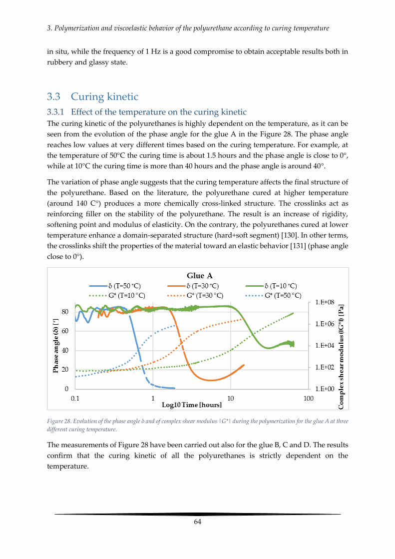
3. Polymerization and viscoelastic behavior of the polyurethane according to curing temperature
64
in situ, while the frequency of 1 Hz is a good compromise to obtain acceptable results both in
rubbery and glassy state.
3.3 Curing kinetic
3.3.1 Effect of the temperature on the curing kinetic
The curing kinetic of the polyurethanes is highly dependent on the temperature, as it can be
seen from the evolution of the phase angle for the glue A in the Figure 28. The phase angle
reaches low values at very different times based on the curing temperature. For example, at
the temperature of 50°C the curing time is about 1.5 hours and the phase angle is close to 0°,
while at 10°C the curing time is more than 40 hours and the phase angle is around 40°.
The variation of phase angle suggests that the curing temperature affects the final structure of
the polyurethane. Based on the literature, the polyurethane cured at higher temperature
(around 140 C°) produces a more chemically cross-linked structure. The crosslinks act as
reinforcing filler on the stability of the polyurethane. The result is an increase of rigidity,
softening point and modulus of elasticity. On the contrary, the polyurethanes cured at lower
temperature enhance a domain-separated structure (hard+soft segment) [130]. In other terms,
the crosslinks shift the properties of the material toward an elastic behavior [131] (phase angle
close to 0°).
Figure 28. Evolution of the phase angle δ and of complex shear modulus |G*| during the polymerization for the glue A at three
different curing temperature.
The measurements of Figure 28 have been carried out also for the glue B, C and D. The results
confirm that the curing kinetic of all the polyurethanes is strictly dependent on the
temperature.
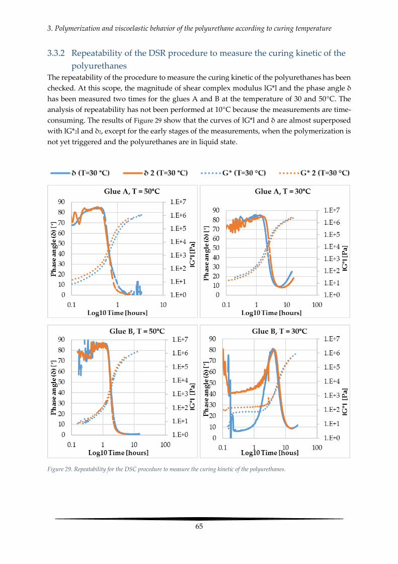
3. Polymerization and viscoelastic behavior of the polyurethane according to curing temperature
65
3.3.2 Repeatability of the DSR procedure to measure the curing kinetic of the
polyurethanes
The repeatability of the procedure to measure the curing kinetic of the polyurethanes has been
checked. At this scope, the magnitude of shear complex modulus lG*l and the phase angle δ
has been measured two times for the glues A and B at the temperature of 30 and 50°C. The
analysis of repeatability has not been performed at 10°C because the measurements are time-
consuming. The results of Figure 29 show that the curves of lG*l and δ are almost superposed
with lG*2l and δ2, except for the early stages of the measurements, when the polymerization is
not yet triggered and the polyurethanes are in liquid state.
Figure 29. Repeatability for the DSC procedure to measure the curing kinetic of the polyurethanes.
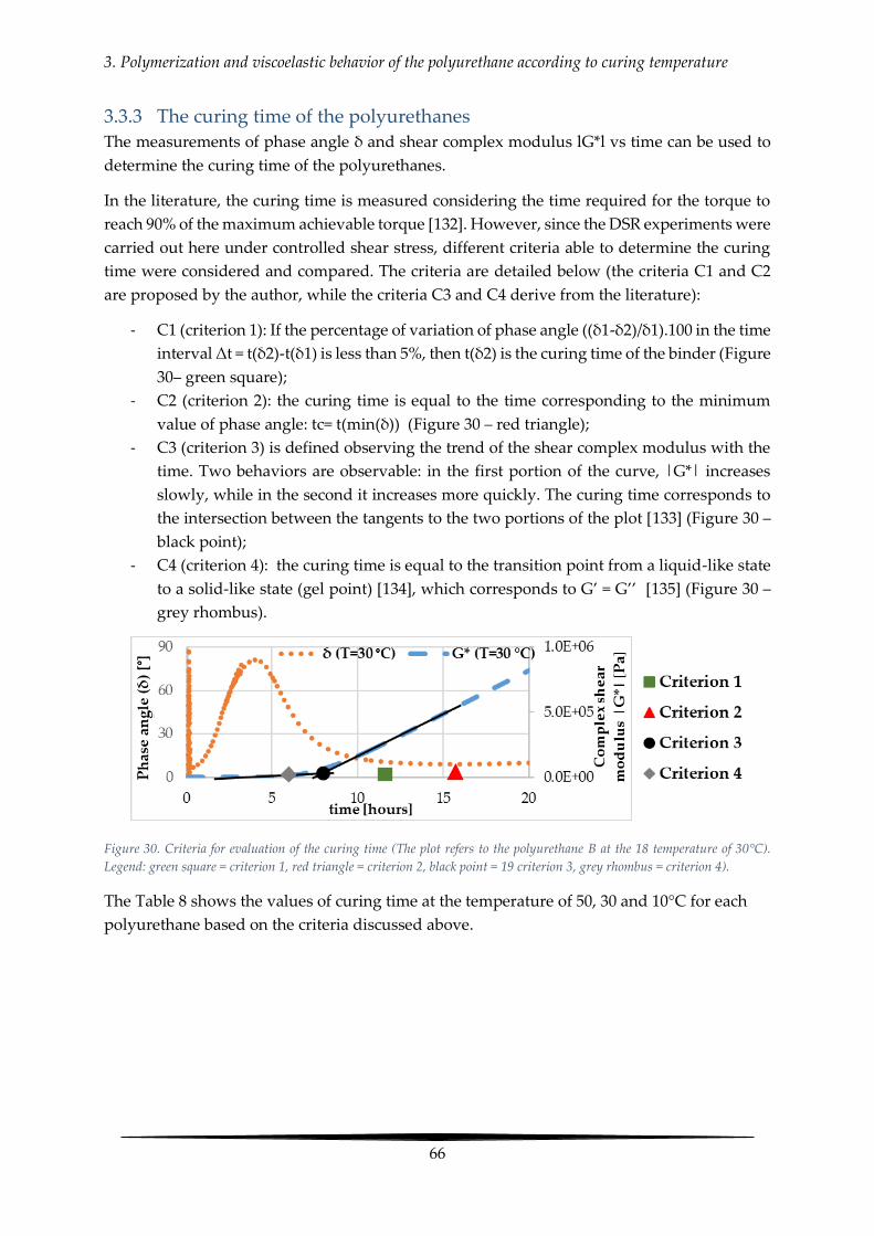
3. Polymerization and viscoelastic behavior of the polyurethane according to curing temperature
66
3.3.3 The curing time of the polyurethanes
The measurements of phase angle δ and shear complex modulus lG*l vs time can be used to
determine the curing time of the polyurethanes.
In the literature, the curing time is measured considering the time required for the torque to
reach 90% of the maximum achievable torque [132]. However, since the DSR experiments were
carried out here under controlled shear stress, different criteria able to determine the curing
time were considered and compared. The criteria are detailed below (the criteria C1 and C2
are proposed by the author, while the criteria C3 and C4 derive from the literature):
- C1 (criterion 1): If the percentage of variation of phase angle ((δ1-δ2)/δ1).100 in the time
interval Δt = t(δ2)-t(δ1) is less than 5%, then t(δ2) is the curing time of the binder (Figure
30– green square);
- C2 (criterion 2): the curing time is equal to the time corresponding to the minimum
value of phase angle: tc= t(min(δ)) (Figure 30 – red triangle);
- C3 (criterion 3) is defined observing the trend of the shear complex modulus with the
time. Two behaviors are observable: in the first portion of the curve, |G*| increases
slowly, while in the second it increases more quickly. The curing time corresponds to
the intersection between the tangents to the two portions of the plot [133] (Figure 30 –
black point);
- C4 (criterion 4): the curing time is equal to the transition point from a liquid-like state
to a solid-like state (gel point) [134], which corresponds to G’ = G’’ [135] (Figure 30 –
grey rhombus).
Figure 30. Criteria for evaluation of the curing time (The plot refers to the polyurethane B at the 18 temperature of 30°C).
Legend: green square = criterion 1, red triangle = criterion 2, black point = 19 criterion 3, grey rhombus = criterion 4).
The Table 8 shows the values of curing time at the temperature of 50, 30 and 10°C for each
polyurethane based on the criteria discussed above.

3. Polymerization and viscoelastic behavior of the polyurethane according to curing temperature
67
Curing time [hours]
Polyu
rethan
e
50 °C 30 °C 10 °C
C1 C2 C3 C4 C1 C2 C3 C4 C1 C2 C3 C4
A 1.5 1.2 0.88 0.64 5.7 9.07 3.95 2.39 29.4 42.5 40.6 NA
B 3.6 3.97 2.24 1.82 13.6 15.6 7.72 6.11 50.6 63.6 45.1 NA
C 3.4 6.11 1.9 NA 5.3 16.1 7.94 NA 33.6 57.8 42.1 14.8
D 8.6 NA 3.43 NA 13.8 NA 13.6 NA 47.1 50.3 50.9 14.8
Table 8. Curing time of the polyurethanes at different temperatures based on four criteria.
The limit of the criterion 1 is the arbitrariness of Δt, which depends on the speed of
polymerization and must be chosen in order to make plausible the 5% limit of phase angle
variation.
Regarding the criterion 2, the limit is in the poor precision of phase angle measurements.
In addition the criterion 4 is not always applicable, because some polyurethanes never reach
the condition G’=G’’, in other terms they show a dominant viscous behavior (G’’ ˃ G’) during
all the curing process. In light of this, the most reliable criterion is the number 3.
Whatever the tested glue, at the temperature of 10°C, the curing time ranges between 30 and
60 hours, while at 50°C it ranges between 1 and 3.5 hours. These results will have to be taken
into account for an implementation of those materials for pavement applications: an
implementation during hot season is clearly advised.
3.3.4 Modeling the curing time through the Arrhenius law
In general, the rate of a reaction is influenced by the temperature or the presence of a catalyst.
In the case of the polyurethane, the reaction involves the diisocyanate and the polyol in the
formation of the urethane. The effect of the temperature on the speed of the reaction is taken
into account by the Arrhenius law [136]:
𝑘 = 𝛥𝑒−𝐸/𝑅𝑇 28
Where: k is the rate constant (sec-1) for a reaction of the first order; E is the activation energy
(J/mol), R is the universal gas constant (8.314 J/K*mol); Δ is a pre-exponential factor (sec-1); T
is the temperature (K). In particular the parameters E and Δ regulate the speed of the reaction.
The empirical nature of the Arrhenius law implies that the rate constant is experimentally
measured at different temperatures.
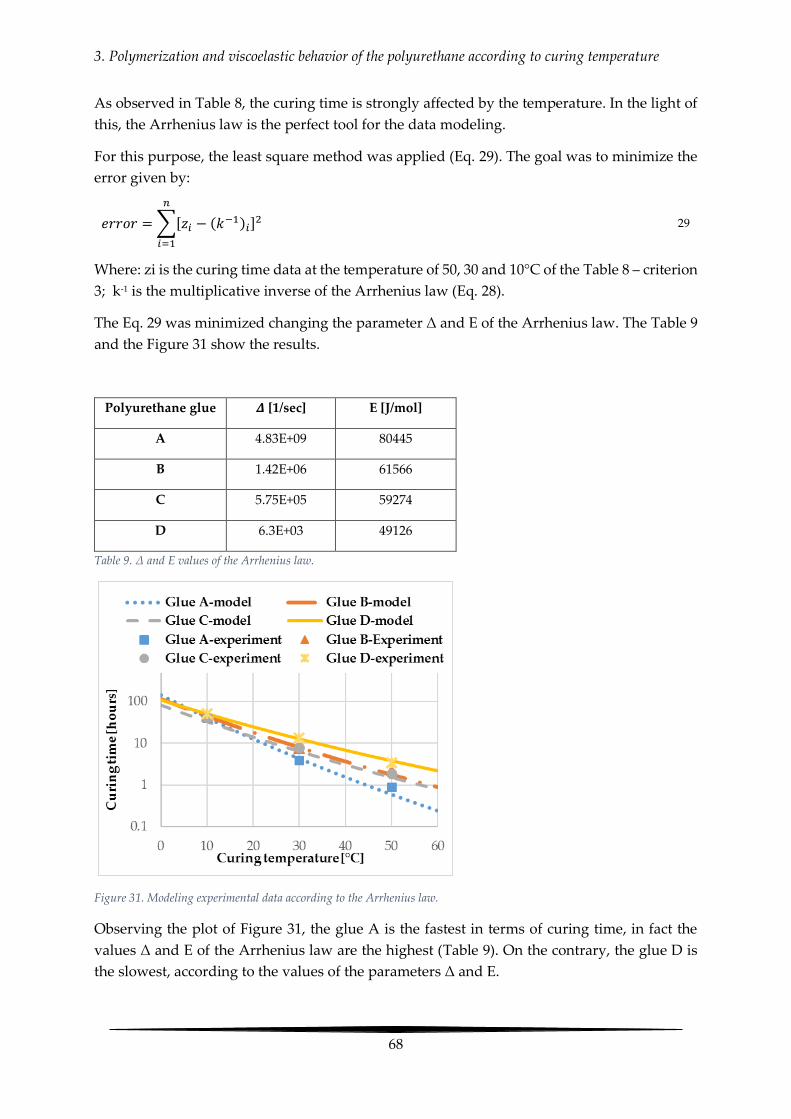
3. Polymerization and viscoelastic behavior of the polyurethane according to curing temperature
68
As observed in Table 8, the curing time is strongly affected by the temperature. In the light of
this, the Arrhenius law is the perfect tool for the data modeling.
For this purpose, the least square method was applied (Eq. 29). The goal was to minimize the
error given by:
𝑒𝑟𝑟𝑜𝑟 =∑[𝑧𝑖 − (𝑘−1)𝑖]
2
𝑛
𝑖=1
29
Where: zi is the curing time data at the temperature of 50, 30 and 10°C of the Table 8 – criterion
3; k-1 is the multiplicative inverse of the Arrhenius law (Eq. 28).
The Eq. 29 was minimized changing the parameter Δ and E of the Arrhenius law. The Table 9
and the Figure 31 show the results.
Polyurethane glue 𝜟 [1/sec] E [J/mol]
A 4.83E+09 80445
B 1.42E+06 61566
C 5.75E+05 59274
D 6.3E+03 49126
Table 9. Δ and E values of the Arrhenius law.
Figure 31. Modeling experimental data according to the Arrhenius law.
Observing the plot of Figure 31, the glue A is the fastest in terms of curing time, in fact the
values Δ and E of the Arrhenius law are the highest (Table 9). On the contrary, the glue D is
the slowest, according to the values of the parameters Δ and E.
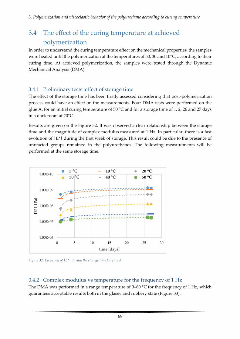
3. Polymerization and viscoelastic behavior of the polyurethane according to curing temperature
69
3.4 The effect of the curing temperature at achieved
polymerization In order to understand the curing temperature effect on the mechanical properties, the samples
were heated until the polymerization at the temperatures of 50, 30 and 10°C, according to their
curing time. At achieved polymerization, the samples were tested through the Dynamic
Mechanical Analysis (DMA).
3.4.1 Preliminary tests: effect of storage time
The effect of the storage time has been firstly assessed considering that post-polymerization
process could have an effect on the measurements. Four DMA tests were performed on the
glue A, for an initial curing temperature of 50 °C and for a storage time of 1, 2, 26 and 27 days
in a dark room at 20°C.
Results are given on the Figure 32. It was observed a clear relationship between the storage
time and the magnitude of complex modulus measured at 1 Hz. In particular, there is a fast
evolution of |E*| during the first week of storage. This result could be due to the presence of
unreacted groups remained in the polyurethanes. The following measurements will be
performed at the same storage time.
Figure 32. Evolution of |E*| during the storage time for glue A.
3.4.2 Complex modulus vs temperature for the frequency of 1 Hz
The DMA was performed in a range temperature of 0–60 °C for the frequency of 1 Hz, which
guarantees acceptable results both in the glassy and rubbery state (Figure 33).
1.00E+06
1.00E+07
1.00E+08
1.00E+09
1.00E+10
0 5 10 15 20 25 30
IE*I
[P
a]
time [days]
5 °C 10 °C 20 °C
30 °C 40 °C 50 °C

3. Polymerization and viscoelastic behavior of the polyurethane according to curing temperature
70
Figure 33. Complex modulus vs temperature for different polyurethanes cured at 50 °C.
The Figure shows that the glues behave like thermoset polymers. At low temperatures (<0°C),
it is reasonable to assume that the polyurethanes are in the glassy region, characterized by a
complex modulus higher than 1E + 9 Pa [137]. As the temperature increases (>0 °C), the
modulus falls through the glass transition region where the glues behave like a viscoelastic
material and the complex modulus is temperature dependent. At higher temperatures, the
polyurethanes are in the rubbery plateau region and the complex modulus stabilizes [138].
More in details, for the glue A and B, the rubbery plateau region starts around 30 °C and the
complex modulus is around 1E + 7 Pa, while the glue C and D are still in the glass transition
region. In comparison with a typical bitumen 35–50, the polyurethanes A, C, and D are stiffer,
especially for temperatures higher than 20 °C.
The glue B is similarly independent of the temperature (complex moduli of 1E + 8 to 1E + 7
Pa). For the conventional asphalt binder, it changes a lot (complex moduli of 1E + 8 to 1E + 4
Pa).
In the perspective of an application in situ, this result is encouraging, considering that a solar
road could be built in hot areas, having very high temperatures during the summertime.
The different modulus and glass transition region of the glues are due to their chemical
composition. Considering for example the glue A and B, they are both thermoset
polyurethanes, but they are composed by different type of diisocyanate having different molar
mass: the 1,6 hexane around 168 gr/mol and the 1,6 hexane homopolymer around 500 gr/mol.
In general, long not-branched molecules yield flexibility and reduce the stiffness of the
polyurethane. That would explain the bigger modulus of the glue A compared to glue B.
Glue C and glue D are special type of polyurea called polyaspartic, which form urea instead
of urethane linkages. In comparison with polyurethane A and B, the polyaspartics exhibit
better mechanical properties and the glass transition regions shift at higher temperatures [123],
as confirmed in Figure 33.
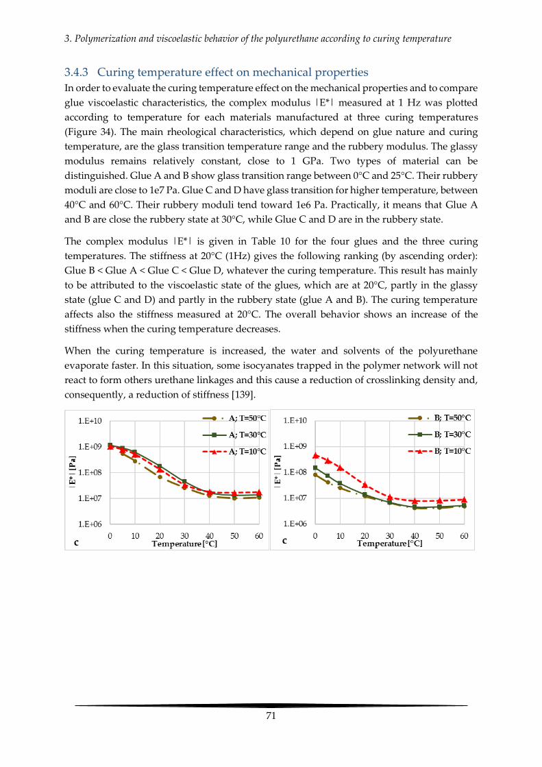
3. Polymerization and viscoelastic behavior of the polyurethane according to curing temperature
71
3.4.3 Curing temperature effect on mechanical properties
In order to evaluate the curing temperature effect on the mechanical properties and to compare
glue viscoelastic characteristics, the complex modulus |E*| measured at 1 Hz was plotted
according to temperature for each materials manufactured at three curing temperatures
(Figure 34). The main rheological characteristics, which depend on glue nature and curing
temperature, are the glass transition temperature range and the rubbery modulus. The glassy
modulus remains relatively constant, close to 1 GPa. Two types of material can be
distinguished. Glue A and B show glass transition range between 0°C and 25°C. Their rubbery
moduli are close to 1e7 Pa. Glue C and D have glass transition for higher temperature, between
40°C and 60°C. Their rubbery moduli tend toward 1e6 Pa. Practically, it means that Glue A
and B are close the rubbery state at 30°C, while Glue C and D are in the rubbery state.
The complex modulus |E*| is given in Table 10 for the four glues and the three curing
temperatures. The stiffness at 20°C (1Hz) gives the following ranking (by ascending order):
Glue B < Glue A < Glue C < Glue D, whatever the curing temperature. This result has mainly
to be attributed to the viscoelastic state of the glues, which are at 20°C, partly in the glassy
state (glue C and D) and partly in the rubbery state (glue A and B). The curing temperature
affects also the stiffness measured at 20°C. The overall behavior shows an increase of the
stiffness when the curing temperature decreases.
When the curing temperature is increased, the water and solvents of the polyurethane
evaporate faster. In this situation, some isocyanates trapped in the polymer network will not
react to form others urethane linkages and this cause a reduction of crosslinking density and,
consequently, a reduction of stiffness [139].
a c c

3. Polymerization and viscoelastic behavior of the polyurethane according to curing temperature
72
Figure 34. Complex modulus |E for different curing temperatures at frequency of 1Hz.
Glue type Tcure=10°C Tcure=30°C Tcure=50°C
|E*| [Pa]
(20°C; 1Hz)
A 1.35*108 1.81*108 6.78*107
B 3.33*107 1.38*107 1.19*107
C 1.57*109 1.97*108 4.53*108
D 1.41*109 5.7*108 5.7*108
Table 10. Complex modulus at 1 Hz and 20°C for each glue, at different curing temperatures.
Another useful plot is the Black diagram, which is a representation of the magnitude of the
complex modulus |E*|, versus the phase angle δ. It gives the overall rheological signature of
a material [139]. The right part of the graph refers to the case of “high temperatures – low
frequencies”, while the left part to the “low temperatures – high frequencies”. Regarding the
plots in Figure 35, the Black curve of the bitumen was introduced for comparison with the
Black curves of the polyurethanes. The smooth curve of the bitumen is an indicator of the time-
temperature equivalency. In the high frequencies – low temperatures domain, the bitumen
exhibits an elastic-like behavior (0° ˂ δ ˂ 20°). At the opposite, in the low frequency-high
temperature domain, it behaves like a Newtonian fluid (δ ≈ 90°). Polyurethanes exhibit also a
continuous curve in the Black diagram showing they can be considered as thermo-
rheologically simple materials. On other words, the macromolecular structure of these
polyurethanes remains stable across temperature, without phase changing (except second
order phase change like glass transition).
The Black curves referring to the polyurethanes binders never reach the value of δ = 90°. The
reason comes from the cross-linked three-dimensional, covalently-bonded structure of the
polyurethanes [141]. Indeed, these materials are non-fusible after curing. In the domain of low
temperatures – high frequencies, all the curves tend to a value of lE*l≈1 GPa. The
polyurethanes are in the glassy state, in fact the phase angle is close to zero degree and the
viscous component of the complex modulus is negligible (lE*l≈ E’). This result is a typical value
of a polymer in glassy state [141], confirming the reliability of the tests. Observing the
e g h
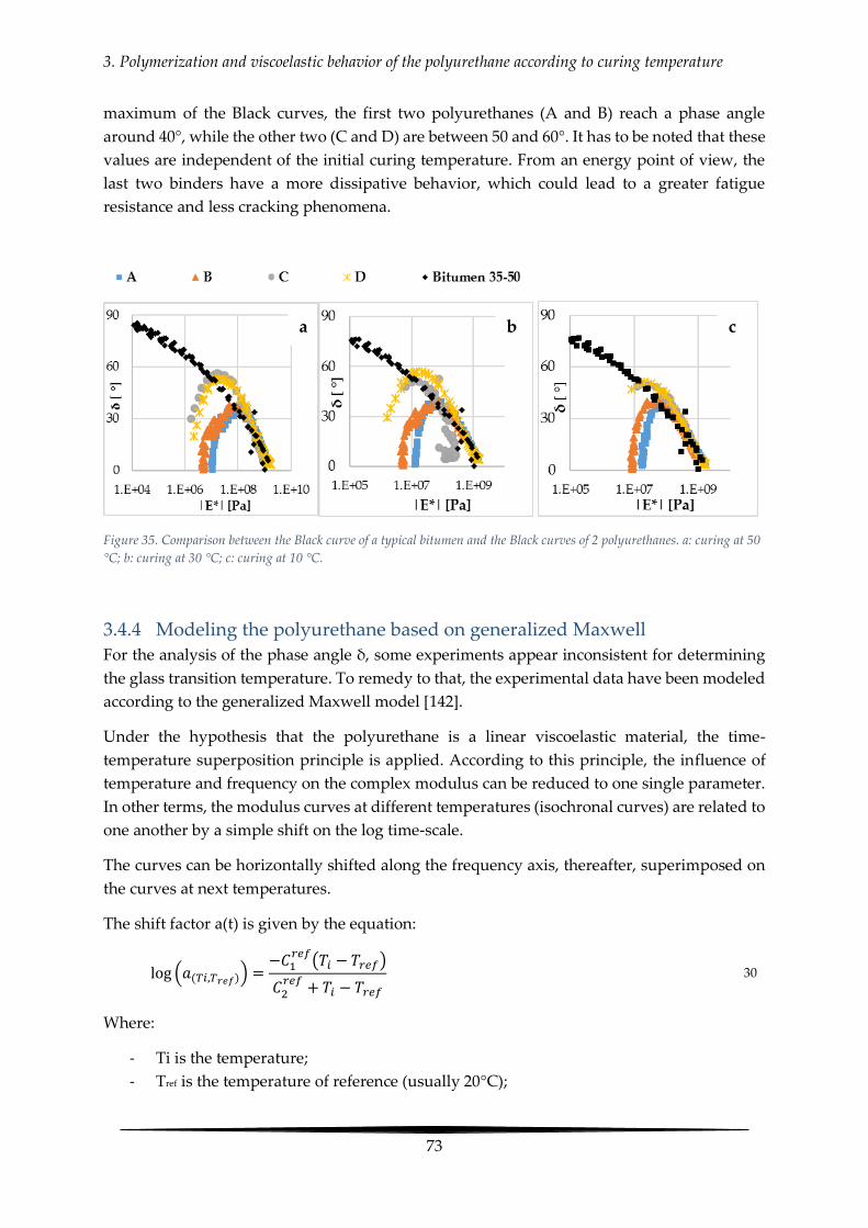
3. Polymerization and viscoelastic behavior of the polyurethane according to curing temperature
73
maximum of the Black curves, the first two polyurethanes (A and B) reach a phase angle
around 40°, while the other two (C and D) are between 50 and 60°. It has to be noted that these
values are independent of the initial curing temperature. From an energy point of view, the
last two binders have a more dissipative behavior, which could lead to a greater fatigue
resistance and less cracking phenomena.
Figure 35. Comparison between the Black curve of a typical bitumen and the Black curves of 2 polyurethanes. a: curing at 50
°C; b: curing at 30 °C; c: curing at 10 °C.
3.4.4 Modeling the polyurethane based on generalized Maxwell
For the analysis of the phase angle δ, some experiments appear inconsistent for determining
the glass transition temperature. To remedy to that, the experimental data have been modeled
according to the generalized Maxwell model [142].
Under the hypothesis that the polyurethane is a linear viscoelastic material, the time-
temperature superposition principle is applied. According to this principle, the influence of
temperature and frequency on the complex modulus can be reduced to one single parameter.
In other terms, the modulus curves at different temperatures (isochronal curves) are related to
one another by a simple shift on the log time-scale.
The curves can be horizontally shifted along the frequency axis, thereafter, superimposed on
the curves at next temperatures.
The shift factor a(t) is given by the equation:
log (𝑎(𝑇𝑖,𝑇𝑟𝑒𝑓)) =−𝐶1
𝑟𝑒𝑓(𝑇𝑖 − 𝑇𝑟𝑒𝑓)
𝐶2𝑟𝑒𝑓
+ 𝑇𝑖 − 𝑇𝑟𝑒𝑓 30
Where:
- Ti is the temperature;
- Tref is the temperature of reference (usually 20°C);
a b c
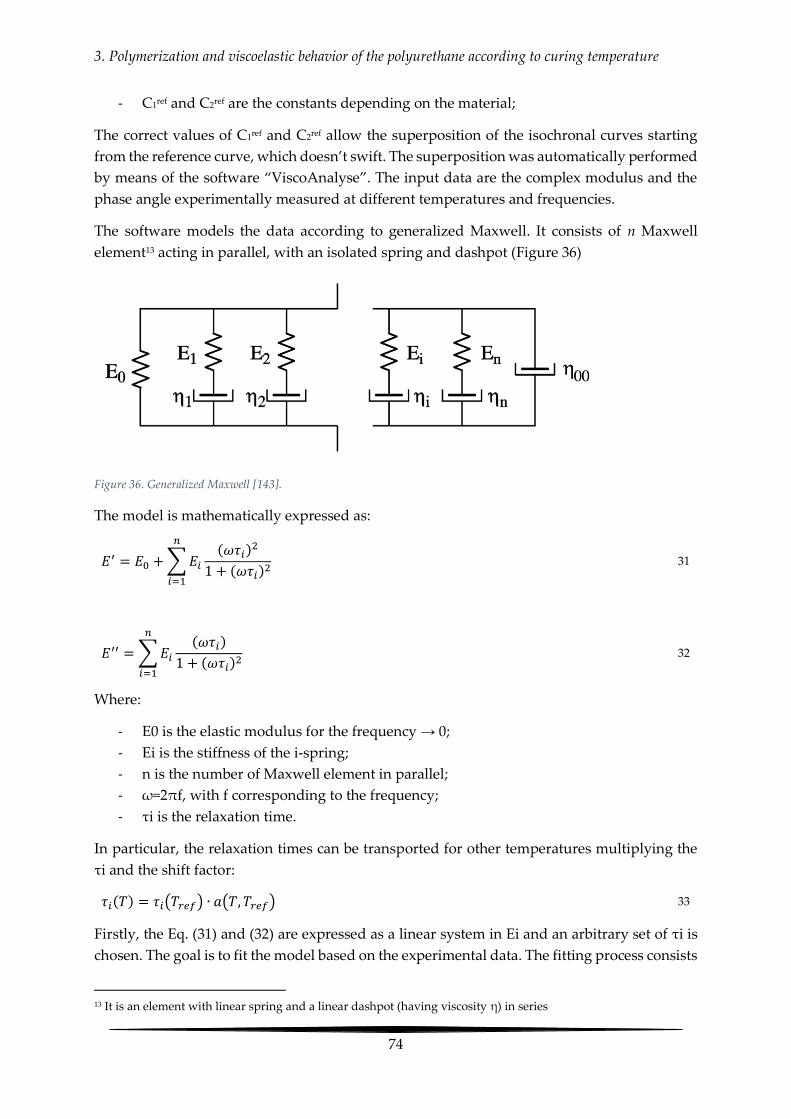
3. Polymerization and viscoelastic behavior of the polyurethane according to curing temperature
74
- C1ref and C2ref are the constants depending on the material;
The correct values of C1ref and C2ref allow the superposition of the isochronal curves starting
from the reference curve, which doesn’t swift. The superposition was automatically performed
by means of the software “ViscoAnalyse”. The input data are the complex modulus and the
phase angle experimentally measured at different temperatures and frequencies.
The software models the data according to generalized Maxwell. It consists of n Maxwell
element13 acting in parallel, with an isolated spring and dashpot (Figure 36)
Figure 36. Generalized Maxwell [143].
The model is mathematically expressed as:
𝐸′ = 𝐸0 +∑𝐸𝑖(𝜔𝜏𝑖)
2
1 + (𝜔𝜏𝑖)2
𝑛
𝑖=1
31
𝐸′′ =∑𝐸𝑖(𝜔𝜏𝑖)
1 + (𝜔𝜏𝑖)2
𝑛
𝑖=1
32
Where:
- E0 is the elastic modulus for the frequency → 0;
- Ei is the stiffness of the i-spring;
- n is the number of Maxwell element in parallel;
- ω=2πf, with f corresponding to the frequency;
- τi is the relaxation time.
In particular, the relaxation times can be transported for other temperatures multiplying the
τi and the shift factor:
𝜏𝑖(𝑇) = 𝜏𝑖(𝑇𝑟𝑒𝑓) ∙ 𝑎(𝑇, 𝑇𝑟𝑒𝑓) 33
Firstly, the Eq. (31) and (32) are expressed as a linear system in Ei and an arbitrary set of τi is
chosen. The goal is to fit the model based on the experimental data. The fitting process consists
13 It is an element with linear spring and a linear dashpot (having viscosity η) in series

3. Polymerization and viscoelastic behavior of the polyurethane according to curing temperature
75
of an optimization based on the least square method. The output is E0, τi and Ei at the reference
temperature.
The modeling was performed for all the glues, plotting the variation of E’, E’’ and tan(δ)
according to the temperature, for a frequency of 1 Hz. The curves for the glue A are presented
Figure 37, while the curves for the other glues are in the Annex 6.

3. Polymerization and viscoelastic behavior of the polyurethane according to curing temperature
76
Figure 37. Modeling of E’, E’’ and tan(δ) according to generalized Maxwell for the glue A.

3. Polymerization and viscoelastic behavior of the polyurethane according to curing temperature
77
Reminding that the tangent of the phase angle δ is given by the ratio between E’’ and E’
(tan(δ)=E’’/E’), the glass transition temperature (Tg) is defined as the temperature
corresponding to max of tan(δ) [144]. Calculus is performed on the theoretical curve, using the
software Scilab.
Glue type Tcure=10°C Tcure=30°C Tcure=50°C ΔTg=Tgcure10-
Tgcure50
Tg ( °C)
A 23.4 26.2 15.7 7.7
B 14.7 8.3 -0.5 15.2
C 56 61.4 44.5 11.5
D 55.4 44.1 43.2 12.2
Table 11. Glass transition temperature at different curing temperature.
Based on Nabeth et al [145], the Tg is function of the network structure and it depends on the
composition of the polyurethane, the curing agent, the curing time, the cross-linking density
and the temperature. More in detail, the Tg increases according to the crosslinks, or with the
increase of hard segment content [146]. This observation is confirmed by the measurements of
Table 11. The glue B, composed by long-chain molecules, has the lower crosslinks density and
the lower Tg. Vice-versa the glue C, which is a high-stiffness polyaspartic, has the higher
crosslinks density and the higher Tg.
Curing temperature appears to have a non-negligible effect on Tg. In general, more the curing
temperature increases, less is Tg. Observing the variation of glass transition from 10 to 50°C of
curing, the glue A is the less affected, while the B is the most.
3.4.5 Discussion
Based on the results, the temperature affects not only the speed of the reaction between the
diisocyantes and the polyols, but also the final structure of polyurethane. In general, the
increase of the curing temperature produces a more chemically cross-linked structure. Higher
curing temperature could also promote the quick evaporation of the solvents. Consequently,
some disocyanates trap in the polymer network and they don’t react with the polyols, causing
a reduction of stiffness.
Lower temperature promotes the full reaction of the diisocyanates with the polyols, leading
the polyurethane towards a segmented structure.
The energy of activation during the polymerization is affected by the presence of catalysts. For
example, the glue B has a lower energy of activation in comparison with the glue A thanks to
the catalyst dibutyltin dilaurate.
At same curing temperature, the polyurethanes show different modulus and Tg because of
their different chemical composition. In general, longer not-branched molecules enhance the

3. Polymerization and viscoelastic behavior of the polyurethane according to curing temperature
78
flexibility, but reduce the crosslinks density and, consequently, the stiffness. This type of
behavior can be qualitatively detected by the Tg. In fact, higher values of Tg are associated
with a cross-linked structure (high concentration of urethane groups).
Also the solvents play an important role on the final structure of the polyurethane. Firstly, they
affect the viscosity of the materials before triggering of the polymerization. For example, in the
glue C, the reaction between amines and isocyanates is very quick. In this case, the toluene
and xylene are able to modify the rate of reaction, increasing the pot time and improving the
workability of the glue.
Regarding the glue C and D, they are special type of polyurea called polyaspartic, which
exhibit higher stiffness in comparison with the polyurethane. The polyaspartics form urea
instead of urethane linkages and they have a longer pot life in comparison with typical
polyurea.
From an energy point of view, the glue C and D have a more dissipative behavior, which could
lead to a greater fatigue resistance and less cracking phenomena.
3.5 Conclusions In this chapter, four different types of polyurethanes, good candidate to act as transparent
binder for pavement surface mixes, were characterized in terms of curing time and viscoelastic
behavior. For this purpose, an experimental campaign was conducted performing two types
of test: the Dynamic Shear Rheometer and the Dynamic Mechanical Analysis.
The results demonstrated the strong dependency of the curing time on the curing temperature.
For example, at the temperature of 10°C, the curing time ranges between 30 and 60 hours,
while at 50°C it ranges between 1 and 3.5 hours. According to this, any outdoors applications
should be carried out during summer time, when the average temperature is higher.
For a better comprehension of the curing, the experimental data were modelled according to
the Arrhenius law and for each binder an equation was derived. Large differences in curing
time were observed for each type of glue with activation energy ranging from 80445 J/mol
(Glue A) to 49126 J/mol (Glue D).
Once the polymerization was achieved, the variation of the complex modulus according to the
temperature was studied. It was observed that reducing the curing temperature the complex
modulus increases (measured at 20°C, 1 Hz). This result is mainly due to the position of the
glass transition, which is different for each glue. At the temperature of 20°C, the first two
polyurethanes (A and B) were in the glass transition temperature range, while the two
remaining (C and D) were in glassy state. From a chemical point of view, the reduction of
stiffness occurs because higher curing temperatures generate polyurethanes with lower
urethanes group, lower cross-linking density and increased amounts of residual interlocked
isocyanates.
3. Polymerization and viscoelastic behavior of the polyurethane according to curing temperature
79
The evolution of the complex modulus with the storage time of the samples was also
investigated. The plot showed a quick increase of |E*| during the first week of storage,
probably due to the continuation of the polymerization because of unreacted isocyanates
groups remained in the glue.
Residual isocyanates may also affect the long term durability of the polyurethane and elevated
temperatures could allow the reactions of isocyanate to continue unexpectedly. The formation
of other covalent bonds reduces the average distance between atoms, and it could cause
shrinkage or increased stress in the polyurethane.
In comparison to conventional bitumen 35-50, the polyurethanes showed the typical behavior
of a thermoset polymer. Indeed, analyzing the Black curves, in the domain of high
temperatures – low frequencies the polyurethanes never reached the Newtonian state (phase
angle of 90°). Polyurethanes reach a maximum value of phase angle around 40° for the glue A
and B and between 50° and 60° for the glue C and D. The right branches of the Black curves
(low temperature – high frequency) are very similar both for the bitumen and the
polyurethanes.
The Tg, obtained after modeling through “generalized Maxwell model”, follows the ranking
B˂A˂D˂C. This order is consistent with the structure of the polyurethanes: the glue B has the
lowest Tg and also the lowest complex modulus (low crosslinks density), vice-versa the glue
C has the highest Tg and high complex modulus (high crosslinks density).
The knowledge of the curing conditions will be helpful for outdoor applications. For example,
the average temperature in Reggio Calabria (South of Italy) during the month of August is
27°C. In this condition, the glue A would be the fastest in terms of curing time (5.8 hours) and
it would operate close to the glass transition temperature.


4. The semi-transparent layer design
81
4. The semi-transparent layer design The semi-transparent layer used in solar roads plays a fundamental role because it has to
support the traffic load, guarantee the vehicles friction, protect the solar cells, allow the
passage of the sunlight and maximize the heat transfer in layer containing heat-transfer fluid.
In the present study, the proposed semi-transparent layer is a composite material made of
recycled glass aggregates bonded together using the polyurethane glues studied in the chapter
3.
The semi-transparent layer design has been carried out based on three different approaches:
the “packing density” in a preliminary step, the “fraction factorial design” to understand and
quantify all the design parameters and the “surface dressing” as the final stage. There are
respectively called STL1, STL2 and STL3.
With STL1, the influence of each variable (type of glue, grading curve and glue content) on the
optical and mechanical performance of the semi-transparent layer was studied. With STL2, the
mix-design is detailed and oriented to the optimization of all the parameters, in order to
maximize the performance of the material. Moving from the observations outlined with the
STL1 and STL2, the STL3 reinvents the semi-transparent layer, taking inspiration from the
surface dressing.
4.1 The glass aggregates The aggregates used for this study are recycled glass obtained from perfume bottles, crushed
and selected according to the volume fractions of 4/6mm, 2/4mm and 0/2mm. The grading
curves are given in Figure 38.
Figure 38. Grading curves of the glass fractions.
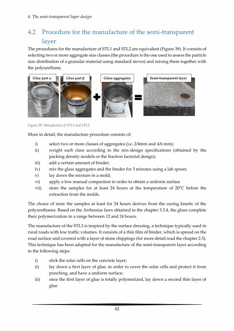
4. The semi-transparent layer design
82
4.2 Procedure for the manufacture of the semi-transparent
layer The procedures for the manufacture of STL1 and STL2 are equivalent (Figure 39). It consists of
selecting two or more aggregate size classes (the procedure is the one used to assess the particle
size distribution of a granular material using standard sieves) and mixing them together with
the polyurethane.
Figure 39. Manufacture of STL1 and STL2.
More in detail, the manufacture procedure consists of:
i) select two or more classes of aggregates (i.e. 2/4mm and 4/6 mm);
ii) weight each class according to the mix-design specifications (obtained by the
packing density models or the fraction factorial design);
iii) add a certain amount of binder;
iv) mix the glass aggregates and the binder for 3 minutes using a lab spoon;
v) lay down the mixture in a mold;
vi) apply a low manual compaction in order to obtain a uniform surface
vii) store the samples for at least 24 hours at the temperature of 20°C before the
extraction from the molds.
The choice of store the samples at least for 24 hours derives from the curing kinetic of the
polyurethanes. Based on the Arrhenius laws obtained in the chapter 3.3.4, the glues complete
their polymerization in a range between 12 and 24 hours.
The manufacture of the STL3 is inspired by the surface dressing, a technique typically used in
rural roads with low traffic volumes. It consists of a thin film of binder, which is spread on the
road surface and covered with a layer of stone chippings (for more detail read the chapter 2.5).
This technique has been adapted for the manufacture of the semi-transparent layer according
to the following steps:
i) stick the solar cells on the concrete layer;
ii) lay down a first layer of glue, in order to cover the solar cells and protect it from
punching, and have a uniform surface;
iii) once the first layer of glue is totally polymerized, lay down a second thin layer of
glue
Glue part α Glue part β Glass aggregates Semi-transparent layer

4. The semi-transparent layer design
83
iv) immediately spread out the glass aggregates and compact it to ensure a penetration
of the aggregate into the fluid layer.
The compaction is very low and it is carried out manually in the laboratory. The success of
this procedure is affected by the amount of glue used for the second layer. The aggregates
have to be not totally immerged in the binder, in order to provide skid resistance to the
surface.
4.3 Evaluation of the mechanical performance: the three-point
bending test The mix-design of the semi-transparent layer requires the evaluation of the mechanical
performance. Because of the high number of samples, the idea was to find a test with the
following characteristic: quickness, simplicity and readiness. Among the numerous tests
recommended by researchers, agencies or standards, the three-point flexural test responds to
these needs.
The three-point flexural test measures the flexural properties of composite materials, including
strength and stiffness [147]. The sample is a bar of 16*2.5*1 cm3, equivalent to a simply
supported beam (Figure 40). The load is applied in the middle of the bar and the loading speed
is constant.
Figure 40. The three-point flexural test.
The test is performed allocating the sample in a water bath in order to control the temperature
and setting the number of cycles, the loading speed and the maximum load (or maximum
deflection).
The test stops automatically if the bar breaks and the final result is the deflection-load behavior
of the material.
Assuming the beam as a homogenous and elastic material simply supported at two points and
loaded in the midpoint, the value of the bending moment in the middle is:
𝑀𝑥 = 𝐹𝐿
4
34

4. The semi-transparent layer design
84
Where F is the load and L is the length of the beam.
The flexural stress can be calculated moving from the de Saint-Venant equation [148]:
𝜎𝑧 =𝑁
𝐴−𝑀𝑦
𝐼𝑦𝑥 +
𝑀𝑥𝐼𝑥𝑦 35
Where:
- Ix and Iy are the cross section inertia moments with respect to the x and y axes;
- Mx and My are the bending moments along the axes x and y, respectively;
- N is the axial force;
- A is the cross section x-y.
Figure 41. Bending of a generalized beam [148].
Under the hypothesis mentioned before (beam simply supported and loaded in the midpoint),
N and My are equal to zero and the Eq. (35) becomes:
𝜎𝑧 =𝑀𝑥𝐼𝑥𝑦 36
In particular, the moment of inertia about x axes is bh3/12 (assuming that the origin of the axes
coincides with the centroid of the cross section) and y is the distance from the neutral axis.
For y=h/2 and 𝑀𝑥 = 𝐹𝐿
4 the Eq. (36) can be written as:
𝜎𝑧 =3𝐹𝐿
2𝑏ℎ2 37
The Eq. (37) is the one proposed in the standard ASTM D7264 [147] to calculate the maximum
flexural stress.
The maximum strain at the outer surface in the mid-span of the beam is given by:

4. The semi-transparent layer design
85
휀 =6𝛿ℎ
𝐿2 38
From the Eq. (37) and (38), the stress-strain curve can be derived (Figure 42).
Figure 42. Example of stress-strain curve.
In the first portion of the curve, the Young Modulus, denoted by the slope of the curve, is low.
During this initial stage, the sample is not well positioned and properly supported, because of
its imperfect geometry. Once the strain increases, the sample tends to stabilize on the supports
and the curve has an evident change of the slope. This slope represents the elastic modulus of
the material. As the strain continues to increase, the material deviates from the elastic to the
plastic domain and it undergoes irreversible deformations. The result is a reduction of the
curve’s slope. Finally, the stress reaches the maximum, corresponding to the rupture of the
sample.
The area given by the stress-strain curve until the rupture (excluding the first part when the
sample is not yet properly supported) represents the toughness, which is the ability of a
material to absorb energy before the rupture.
Summing up, the parameters that can be easily derived from the strain stress curve are:
- σrupture, which is the maximum stress that the samples can withstand before the rupture;
- εrupture, which is the strain corresponding to the maximum stress;
- E, or Young modulus, given by the slope of the curve (excluding the first portion);
- the toughness, corresponding to the area under the stress-strain curve until the
rupture.
4.4 Evaluation of the optical performance: the power loss The optical performance was evaluated in terms of power loss of the pv cells because of the
semi-transparent layer. The scope of this test is to generate the sunlight radiation in a
controlled environment and to measure the power reduction.

4. The semi-transparent layer design
86
The equipment is composed of: i) an halogen lamp of 400 W placed into a box; ii) a pv cell
having dimensions 15 cm*15 cm with a peak power of 15 W, an open circuit voltage Voc of
19.5 V and a short circuit current Isc of 0.97 A in standard conditions (Irradiance of 1000 W/m²
and temperature of 25°C); iii) a solarimeter to check the stability of the radiation during the
test; iv) a set of resistances between 2 and 5000 Ω; v) two multimeters to measure
simultaneously the intensity current and the voltage of the solar cell for each resistance and
vi) a thermometer to control the temperature in the box. The test provides the intensity-voltage
curve of the solar cell (Figure 43) and its maximum power point (see Annexes 1 and 2).
Figure 43. Example of intensity-voltage curve.
The test is then repeated covering the solar cell with the semi-transparent layer and measuring
again the intensity-voltage curve and the maximum power point. Finally, the power loss PL
can be calculated according to the formula:
𝑃𝐿 =(𝑃𝑚𝑎𝑥,𝑢𝑛𝑐 − 𝑃𝑚𝑎𝑥,𝑐)
𝑃𝑚𝑎𝑥,𝑢𝑛𝑐100 39
where:
- Pmax,unc is the maximum power point of the solar cell;
- Pmax,c is the maximum power point of the solar cell covered by the semi-transparent
layer.
The PL ranges theoretically between 0% (top layer perfectly transparent) and 100% (top layer
totally black).

4. The semi-transparent layer design
87
4.4.1 Novel approach modeling the intensity-voltage curve
The intensity-voltage curve of a solar cell is commonly modeled using the single-diode model
[149]. It consists of a current source Il, a diode14 D, a series of resistor Rs and a shunt resistor
Rsh15. More in details:
- Il represents the photogenerated current and it depends on the intensity of the incident
solar radiation, the characteristics of the solar cell and the ambient temperature.
- Rs is the series resistances and it represents the internal losses due to the flow of the
current;
- Rsh is the shunt resistance.
The equation is given by:
𝐼 = 𝐼𝑙 − 𝐼0 (𝑒(𝑉+𝐼∙𝑅𝑠)𝑛∙𝑇 − 1) −
𝑉 + 𝐼 ∙ 𝑅𝑠𝑅𝑠ℎ
40
Where:
- n = diode factor (1 ≤ n ≤ 2);
- T = temperature of the cell (K);
- I0 is the inverse current saturation of the diode.
In this paragraph, a novel approach for modeling the intensity-voltage curve is proposed. The
idea is to build a model starting from the ellipse equation:
(𝑥
𝑎)2
+ (𝑦
𝑏)2
− 1 = 0 41
Assuming: x = Voltage and y = Intensity of current, the (41) becomes:
(𝑉
𝑎)2
+ (𝐼
𝑏)2
− 1 = 0 42
In particular,
- If I=0, (condition for open-circuit voltage Voc) than 𝑉2 = 𝑎2 = 𝑉𝑜𝑐2
- If V=0, (condition for short circuit current Isc) 𝐼2 = 𝑏2 = 𝐼𝑠𝑐2
The Eq. (42) can be written as:
I = 𝐼𝑠𝑐√1 − (𝑉
𝑉𝑜𝑐)2
43
The Eq. (43) can be generalized introducing two parameters a and b:
I = 𝐼𝑠𝑐 (1 − (𝑉
𝑉𝑜𝑐)𝑎
)
𝑏
44
14 It is an electrical component that conducts current in one direction 15 It takes into account impurities near the p-n junction (see Annex 1) of the solar cell

4. The semi-transparent layer design
88
The terms a, b, Isc and Voc can be derived by fitting of the model (44) on the experimental
measurements of intensity and voltage. The goal is to minimize the error given by the least
square method:
𝑒𝑟𝑟𝑜𝑟 =∑(𝐼𝑚𝑜𝑑𝑒𝑙,𝑖 − 𝐼𝑒𝑥𝑝,𝑖)2
𝑛
𝑖=1
45
Where:
- I model,i is the i-th intensity of current obtained through the model (44);
- Iexp,i is the i-th intensity of current measured experimentally;
- n is the number of measurements for building the intensity-voltage curve.
Once the terms a, b, Isc and Voc are calculated, the maximum power point can be derived.
Assuming V=x and I=y (corresponding to the Eq. (44)), the maximum power point MPP is
given by:
𝑀𝑃𝑃 = max[𝑉 ∙ 𝐼] = max[𝑥 ∙ 𝑦] 46
The product x·y represents the power P and it can be written as:
𝑃 = 𝑥 · 𝑦 = 𝐼𝑠𝑐𝑥 (1 − (𝑥
𝑉𝑜𝑐)𝑎
)𝑏
47
The MPP can be obtained calculating the derivative of the eq. (47). In particular:
dP
dx= P′; P′(x0) = 0; P(x0) = MPP 48
Before calculating the derivative, the term (1 − (𝑥
𝑉𝑜𝑐)𝑎)𝑏
of the Eq. (47) can be written according
the binomial expansion.
In general:
(1 + 𝑥)𝑛 = 1 + 𝑛𝑥 +𝑛(𝑛 − 1)𝑥2
2!+𝑛(𝑛 − 1)(𝑛 − 2)𝑥3
3!+ ⋯ 49
Appling the (49) at the second power, the result is:
(1 − (𝑥
𝑉𝑜𝑐)𝑎
)𝑏
= 1 − b(𝑥
𝑉𝑜𝑐)𝑎
+1
2𝑏(𝑏 − 1) (
𝑥
𝑉𝑜𝑐)2𝑎
50
Replacing the Eq. (50) in the Eq. (47), the power of the solar cells becomes:
𝑃 = 𝐼𝑠𝑐𝑥 − 𝐼𝑠𝑐𝑥 ∙ 𝑏 (𝑥
𝑉𝑜𝑐)𝑎
+1
2𝐼𝑠𝑐𝑥 ∙ 𝑏(𝑏 − 1) (
𝑥
𝑉𝑜𝑐)2𝑎
51
Finally, the Eq. (51) can be derived according to the product rule d(f*g) = f’*g + g’*f :
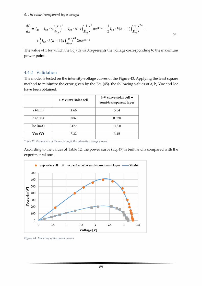
4. The semi-transparent layer design
89
𝑑𝑃
𝑑𝑥= 𝐼𝑠𝑐 − 𝐼𝑠𝑐 ∙ b (
𝑥
𝑉𝑜𝑐)𝑎
− 𝐼𝑠𝑐 ∙ b ∙ 𝑥 (1
𝑉𝑜𝑐)𝑎
𝑎𝑥𝑎−1 +1
2𝐼𝑠𝑐 ∙ 𝑏(𝑏 − 1) (
𝑥
𝑉𝑜𝑐)2𝑎
+
+1
2𝐼𝑠𝑐 ∙ 𝑏(𝑏 − 1)𝑥 (
𝑥
𝑉𝑜𝑐)2𝑎2𝑎𝑥2𝑎−1
52
The value of x for which the Eq. (52) is 0 represents the voltage corresponding to the maximum
power point.
4.4.2 Validation
The model is tested on the intensity-voltage curves of the Figure 43. Applying the least square
method to minimize the error given by the Eq. (45), the following values of a, b, Voc and Ioc
have been obtained.
I-V curve solar cell I-V curve solar cell +
semi-transparent layer
a (dim) 4.66 5.04
b (dim) 0.869 0.828
Isc (mA) 317.6 113.0
Voc (V) 3.32 3.15
Table 12. Parameters of the model to fit the intensity-voltage curves.
According to the values of Table 12, the power curve (Eq. 47) is built and is compared with the
experimental one.
Figure 44. Modeling of the power curves.

4. The semi-transparent layer design
90
The model fits well the data (Figure 44). For example, the MPP of the experimental curve of
the solar cell is 601.6 mW, while the MPP obtained using the model is 615.1 mW, with a
difference of 2%.
4.5 Preliminary Mix-design of the semi-transparent layer
based on the particle packing degree (STL1)
The STL1 is the semi-transparent layer designed according to the particle packing degree. The
idea is to reduce the porosity of the medium and optimize the use of the binder, in order to
increase the strength of the material.
In this paragraph, three different mixtures are tested and the results are compared with a
typical French asphalt.
The mix α derives from some previous preliminary tests mentioned in the chapter 1.2, the mix
β is the result of a packing density optimization based on the De Larrard Model (see chapter
2.2.1.3) and the mix γ is based on the grading curve of a real stone mastic asphalt [150].
In all formulas, the fine particles (<0.064 mm) have not been used, because they could have a
negative impact on the transparency of the semi-transparent layer. In fact, the small
dimensions of the material could interfere with the sunlight wavelengths, reducing the
radiations intercepted by the solar cells.
4.5.1 Mechanical performance
The mechanical performance is evaluated studying the stress-strain curve of the material.
During the three-point flexural test, the sample’s fibers of the lower face undergo a tension
Percentage retained between two sieves
6/10mm[%] 4/6 mm [%] 2/4 mm [%] 0.064/2
mm[%] <0.064 mm[%]
Binder
content [%]
Α 0 57.14 38.1 0 0 4.76
Β 0 0 42.1 53.14 0 4.76
Γ 0 0 61.9 33.3 0 4.76
BBSG 46 2/6 mm [%]
22.5 7.5 5 – 5.5 16
Table 13. Mix design for the STL1.
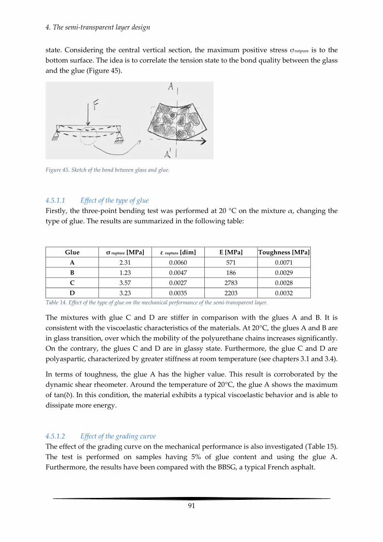
4. The semi-transparent layer design
91
state. Considering the central vertical section, the maximum positive stress σrutpure is to the
bottom surface. The idea is to correlate the tension state to the bond quality between the glass
and the glue (Figure 45).
Figure 45. Sketch of the bond between glass and glue.
4.5.1.1 Effect of the type of glue
Firstly, the three-point bending test was performed at 20 °C on the mixture α, changing the
type of glue. The results are summarized in the following table:
Glue σ rupture [MPa] ε rupture [dim] E [MPa] Toughness [MPa]
A 2.31 0.0060 571 0.0071
B 1.23 0.0047 186 0.0029
C 3.57 0.0027 2783 0.0028
D 3.23 0.0035 2203 0.0032
Table 14. Effect of the type of glue on the mechanical performance of the semi-transparent layer.
The mixtures with glue C and D are stiffer in comparison with the glues A and B. It is
consistent with the viscoelastic characteristics of the materials. At 20°C, the glues A and B are
in glass transition, over which the mobility of the polyurethane chains increases significantly.
On the contrary, the glues C and D are in glassy state. Furthermore, the glue C and D are
polyaspartic, characterized by greater stiffness at room temperature (see chapters 3.1 and 3.4).
In terms of toughness, the glue A has the higher value. This result is corroborated by the
dynamic shear rheometer. Around the temperature of 20°C, the glue A shows the maximum
of tan(δ). In this condition, the material exhibits a typical viscoelastic behavior and is able to
dissipate more energy.
4.5.1.2 Effect of the grading curve
The effect of the grading curve on the mechanical performance is also investigated (Table 15).
The test is performed on samples having 5% of glue content and using the glue A.
Furthermore, the results have been compared with the BBSG, a typical French asphalt.

4. The semi-transparent layer design
92
Mix σ max [Mpa] Toughness [Mpa]
BBSG 6.13 0.1090
Α 2.31 0.0071
Β 1.82 0.0127
Γ 2.60 0.0158
Table 15. Effect of the grading curve on the mechanical performance of the semi-transparent layer.
The mix β and γ shows a clear improvement of toughness in comparison with the mix α, due
to reduction of the porosity in the mixture.
4.5.1.3 Effect of the glue content
Despite the previous mix optimization, the toughness of the asphalt mix remains 10 times
higher than the one obtained for the tested mix so far. For this reason, other experiments have
been performed, increasing the glue content in the formula γ and keeping the same grading
curve and the same type of glue.
Figure 46. Influence of the glue content on the toughness of mix γ.
The results of Figure 46 show an exponential improvement of the mechanical performance
when the glue content increase. In particular, for a glue content around 20 %, the toughness
reaches the same order of magnitude of the asphalt mixture BBSG.
For a glue content higher than 20%, the semi-transparent layer appears smoother, the glue
tends to settle down in the bottom surface and the workability of the mix is reduced.
4.5.2 Optical performance
In terms of optical performance, the power loss has been measured on the mixture α for a glue
content of 5 % and a thickness of 1 cm. The mixtures β and γ have not been tested because

4. The semi-transparent layer design
93
their transparency is greatly affected by the glass fraction 0.064/2 mm. The results are listed in
Table 16.
Type of glue Power loss [%]
A 64.7
B 67.6
C 67.0
D 67.3
Table 16. Effect of the type of glue on the power loss.
The measurements are similar to the one performed for the COP21 demonstrator (see chapter
1.2). In general, type of glue seems to not have a big influence on the power loss of the semi-
transparent layer. Instead, the effect of the glue content and of the thickness is more evident,
as observed in Figure 47.
Figure 47. Effect of glue content and thickness on the power loss.
All the measurements have been performed on the mixture α, using the glue C. More in detail,
the dots refer to the measurements of samples having thickness of 1 cm, while the squares refer
to the thickness of 0.5 cm. The experimental measurements have been fitted according to the
following analytical curve:
𝑃𝐿 =𝑃𝐿𝑔𝑙𝑢𝑒100 ∗ 𝐺𝐶 + 𝑎
𝑏 ∗ 𝐺𝐶 53
Where:
- PL is the power loss [%];
- PLglue100 is the power loss for the mixture made only of glue;
- GC is the glue content [%];
- a and b are two parameters depending on the thickness, on the type of glue and on the
grading curve of the glass aggregates, derived using the least square method [dim].

4. The semi-transparent layer design
94
The parameters a and b assume the values of 93.2 and 1.005 for the thickness of 1 cm, 118.1
and 0.886 for the thickness of 0.5 cm.
In reference to the Figure 47, when the glue content is 0%, the solar radiation strikes only the
granular surface of the glass aggregates and, because of its irregularity, the light bounces off
in all the directions. This phenomenon is called diffuse reflection [151]. Increasing the glue
content, the surface of the semi-transparent layer tends to be more regular and the diffuse
reflection reduces. Instead, when reducing the thickness, the power loss reduces. This happens
because the light attenuation is exponential with the path length through which the light is
travelling (Beer –Lamber law [152]).
4.6 Mix-design of the semi-transparent layer based on the
fraction factorial design (STL2) The mechanical and the optical performance of the semi-transparent layer are affected by the
grading curve of the mixture, the glue content and the thickness. For a better-understanding
of the influence of each variable and their interaction, the fraction factorial design is applied
(see chapter 2.2.3). The objective is to describe the optical and the mechanical performance of
the material by means of a multiple regression model and find the optimal mixture.
Firstly, the experimental domain of each variable is defined as detailed in Table 17.
Variables (−1) Level (+1) Level
x1 = glass fraction 4/6 mm (%) 20 60
x2 = glass fraction 2/4 mm (%) 20 60
x3 = glass fraction 0/2 mm (%) 0 50
x4 = glue content (%) 5 20
x5 = thickness (cm) 0.6 1
Table 17. Experimental domain of the variables.
The level −1 and +1 represent the minimum and maximum values of each variable and they
are the boundary of the domains.
The reader could find singular the boundary condition of 0.6 cm for the thickness. It takes into
account the maximum aggregate size of the glass fractions, corresponding to 6 mm.
The choice of using the fraction factorial design is due to the possibility of reducing the number
of experiments. If the full factorial design was applied, the number of experiments would be
equal to 25 = 32 .This approach would be very time-consuming and for this reason the ¼
factorial design was introduced. In other terms, the number of experiments is reduced to 2(5−2)
= 8, cofounding the last two variables as:

4. The semi-transparent layer design
95
𝑥4 = 𝑥1 ∙ 𝑥2 54
𝑥5 = 𝑥1 ∙ 𝑥2 · 𝑥3 55
Based on the previous assumptions, the model matrix �̿� is given by Table 18.
I x1 x2 x3 x1 * x2 = x4 x1 * x3 x2 * x3 x1 * x2 * x3 = x5
Exp1 +1 −1 −1 −1 +1 +1 +1 −1
Exp2 +1 +1 −1 −1 −1 −1 +1 +1
Exp3 +1 −1 +1 −1 −1 +1 −1 +1
Exp4 +1 +1 +1 −1 +1 −1 −1 −1
Exp5 +1 −1 −1 +1 +1 −1 −1 +1
Exp6 +1 +1 −1 +1 −1 +1 −1 −1
Exp7 +1 −1 +1 +1 −1 −1 +1 −1
Exp8 +1 +1 +1 +1 +1 +1 +1 +1
Table 18. Model matrix
+1 and −1 represent the extreme values of each variable (defined in the Table 17), while the
column I, containing only +1, is used to compute the average response of the system and it is
necessary to obtain a square matrix.
Replacing the terms of the model matrix (Table 18) with the extreme values of each variable,
the following experiments were derived (Table 19).
Experiment n. x1 = 4/6 mm
(%)
x2 = 2/4 mm
(%)
x3 = 0/2 mm
(%)
x4 = glue
(%)
x5 = thickness
(cm)
1 33.3 33.3 0 33.3 0.6
2 70.6 23.5 0 5.9 1
3 23.5 70.6 0 5.9 1
4 42.8 42.8 0 14.4 0.6
5 18.2 18.2 45.4 18.2 1
6 44 15 37 4 0.6
7 15 44 37 4 0.6
8 31.6 31.6 26.3 10.5 1
Table 19. Mix-design of each experiment.

4. The semi-transparent layer design
96
4.6.1 Optical performance
Once the mixes tested were defined based on the fraction factorial design, the influence of
thickness, glue content and grading curve on the optical performance of the semi-transparent
layer has been evaluated. The test is performed twice for each experiment and the average is
calculated. The test is carried out on samples having dimensions of 160 * 160 * 10 mm3 or 160
* 160 * 6 mm3.
The optical performance is calculated in terms of power loss of the solar cell because of the
semi-transparent layer, according to the same procedure of the chapter 4.4.
The test is performed for each mix of Table 19, and the values of power loss are the elements
which form the vector �̅� of the equation y̅ = X̿a̅ + e̅ (see chapter 2.2.3)
Experiment n. Power Loss (%)
1 44.8
2 69.0
3 65.0
4 43.1
5 69.7
6 74.2
7 76.4
8 73.1
Table 20. Vector y ̅ containing the value of power loss measured for each mix.
Based on the results of the Table 20, the vector �̅� can be derived and the regression model
describing the optical performance of the semi-transparent layer is given by:
𝑦 = 64.41 + 0.437𝑥1 − 0.012𝑥2 + 8.937𝑥3 − 6.737𝑥4 − 0.141𝑥1𝑥2 + 1.412𝑥2𝑥3 + 4.787𝑥5 56
The minimum of the regression model, into the domain variables of Table 17, is 42.2% and it
represents the minimum of achievable power loss for the semi-transparent layer.
The solution is given for the following mix-design (Table 21).

4. The semi-transparent layer design
97
Variable Value Mix-design
x1 Glass 4/6 mm −1 20%
x2 Glass 2/4 mm 1 60%
x3 Glass 0/2 mm −1 0%
x4 % glue 1 20%
x5 Thickness −1 0.6 cm
Table 21. Mix-design to minimize the power loss of the semi-transparent layer.
According to the Eq. (56), the influence of each variable on the power loss is reported in Figure
48.
Figure 48. Influence of each mix-design variable on the power loss.
The glass fraction 0.064/2 mm has a negative impact on the power loss of the semi-transparent
layer. In fact, the small dimensions of the aggregates interfere with the sunlight wavelengths,
reducing the radiation intercepted by the solar cells [153, 154].
When the glue content is 0%, the solar radiation strikes only the granular surface and the
diffuse reflection is greater.
As expected, the increase of the thickness reduces the power loss. According the Beer–Lambert
law, for a given medium, the light attenuation is exponential with the path length through
which the light is travelling [152].
To summarize, considering the optical performance, the results show a negative impact for
fine particles and thickness and a positive impact for glue content. Furthermore, the power
loss is more sensitive to the fine particles than the thickness.
4.6.2 Mechanical Performance
The influence of each variable on the mechanical performance is studied following the same
approach described for the optical performance. The mixtures are compared performing the
three- point bending test. The test is performed twice for each experiment and the average is

4. The semi-transparent layer design
98
calculated. The test is carried out at 20 °C, on rectangular samples having dimensions 90 × 25
× 10 mm3 or 90 × 25 × 6 mm3 and calculating the maximum stress in the mid-section.
The toughness has been chosen as the outcome in the fraction factorial design to describe the
mechanical performance of the material. Based on the results of the three-point bending test
on the mixtures listed in Table 19, the vector �̅� is derived (Table 22).
Experiment n. Toughness (MPa)
1 0.1620
2 0.0010
3 0.0017
4 0.0184
5 0.1400
6 0.0006
7 0.0005
8 0.6240
Table 22. Vector �̅� containing the value of toughness measured for each mix.
The regression model, which describes the influence of each variable on the toughness of the
material, is given by Eq. (57):
𝑦 = 0.048 − 0.0278𝑥1 − 0.0276𝑥2 + 0.003𝑥3 + 0.0474𝑥4 + 0.0083𝑥1𝑥2 + 0.0081𝑥2𝑥3 + 0.0029𝑥5 57
The maximum of Eq. (57) is 0.168 MPa and it is the maximum of achievable toughness in the
variables domain of Table 3. The solution is given for the following mix design (Table 23).
Variable Value Mix-design
x1 Glass 4/6 mm −1 37.5%
x2 Glass 2/4 mm −1 37.5%
x3 Glass 0/2 mm −1 0%
x4 % glue 1 25%
x5 Thickness 1 1 cm
Table 23. Mix-design to maximize the toughness of the semi-transparent layer.
According to the Eq. (57), the influence of each variable on the toughness is reported in Figure
49.
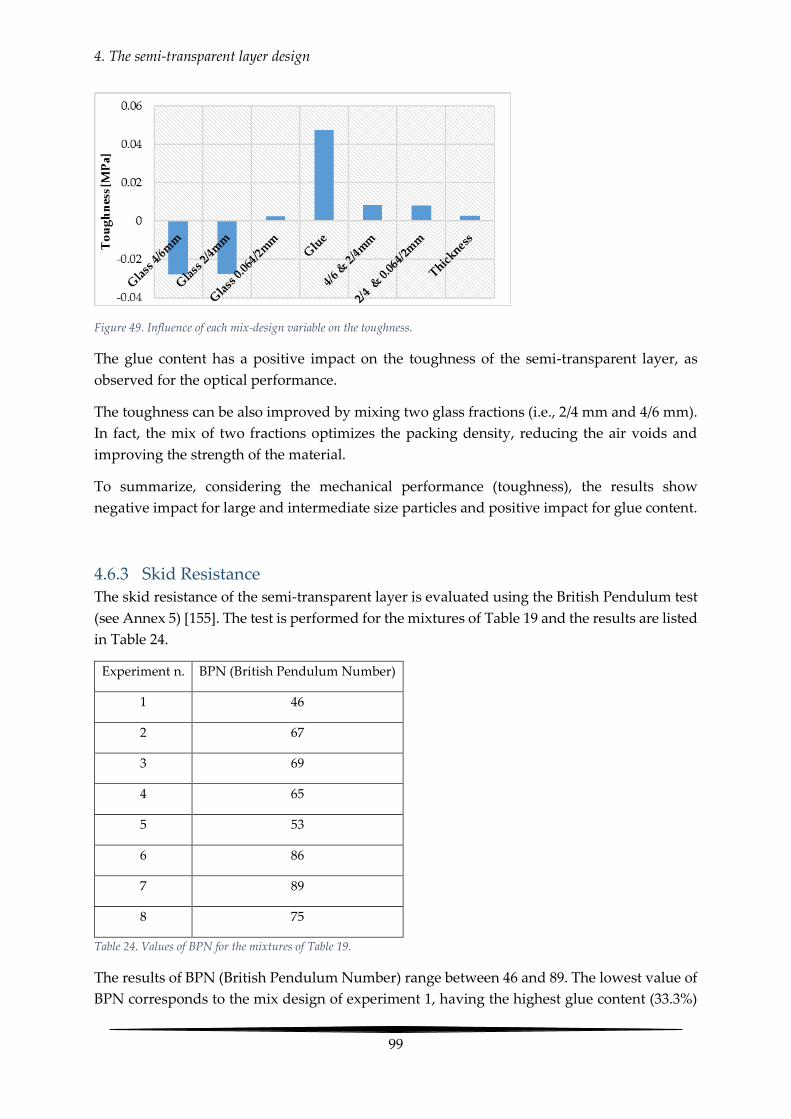
4. The semi-transparent layer design
99
Figure 49. Influence of each mix-design variable on the toughness.
The glue content has a positive impact on the toughness of the semi-transparent layer, as
observed for the optical performance.
The toughness can be also improved by mixing two glass fractions (i.e., 2/4 mm and 4/6 mm).
In fact, the mix of two fractions optimizes the packing density, reducing the air voids and
improving the strength of the material.
To summarize, considering the mechanical performance (toughness), the results show
negative impact for large and intermediate size particles and positive impact for glue content.
4.6.3 Skid Resistance
The skid resistance of the semi-transparent layer is evaluated using the British Pendulum test
(see Annex 5) [155]. The test is performed for the mixtures of Table 19 and the results are listed
in Table 24.
Experiment n. BPN (British Pendulum Number)
1 46
2 67
3 69
4 65
5 53
6 86
7 89
8 75
Table 24. Values of BPN for the mixtures of Table 19.
The results of BPN (British Pendulum Number) range between 46 and 89. The lowest value of
BPN corresponds to the mix design of experiment 1, having the highest glue content (33.3%)

4. The semi-transparent layer design
100
and lowest aggregates in volume. In this condition, the surface appears smoother and not very
homogeneous. Considering that the aggregates provide the skid resistance, the low value of
BPN is consistent with the mix-design of experiment 1. On the other hand, the mix designs of
the experiments 6 and 7 have a BPN of 86 and 89, respectively. In this case, the glue content is
only 4% and the surface is rougher and without smooth parts.
All the other mixtures have a BPN higher than 65, which fulfills the requirements of skid
resistance “even of fast traffic and thus making it most unlikely that the road will be the scene
of repeated accidents” [156].
4.6.4 The Optimal Mixture
Taking into account the results of both optical and mechanical performances, the optimal
mixture will have high glue content, absence of fine particles, and low thickness.
Anyway, the glue content must not exceed 20% in volume, because it will reduce the skid
resistance. The high glue content also causes a reduction of workability of the material. In fact,
the glue tends to settle on the bottom of the mold and the result is a non-homogeneous
mixture.
Based on these observations, the following solution is proposed (Table 25), which corresponds
to experiment number 4 of Table 19.
Variable Mix-design
x1 Glass 4/6 mm 42.8%
x2 Glass 2/4 mm 42.8%
x3 Glass 0/2 mm 0%
x4 % glue 14.4%
x5 Thickness 0.6 cm
Table 25. Optimal mix-design for both mechanical and optical performances.
In comparison with the toughness of the BBSG (0.109 MPa, Table 15), the toughness of the
optimal mix-design is still low (0.0184 MPa, Table 22).
4.7 Mix design of the semi-transparent layer based on the
surface dressing treatment (STL3) The mix designs of the STL1 and STL2 point out the positive impact of the glue content on
both optical and mechanical performances. Unfortunately, the excess of glue content (> 20%)
causes loss of skid resistance and poor workability. The solution to maximize the use of glue,
possibly reducing the thickness, is the surface dressing treatment. As detailed in the chapter
2.2.2, this technique consists of a thin film of binder, which is spread on the road surface and

4. The semi-transparent layer design
101
covered with a layer of stone chippings. For a solar road, the binder is replaced by the
transparent glue, while the stone chippings are replaced by the glass aggregates (see chapter
4.2).
The success of this technique is affected by the amount of glue. The aggregates have not to be
totally immerged into the binder, in order to provide skid resistance to the surface. For this
reason, the packing density of the surface dressing is investigated.
To spread the glass aggregates, a special device is used. It is composed of a tank containing
the glass aggregates and a fluted roller. Pushing forward the device, the aggregates fall from
the tank to the roller and are then pushed down on the surface. The result is a single layer of
aggregates spread out uniformly (Figure 50).
Figure 50. Device for the aggregate spreading.
The repeatability of the device is evaluated in terms of surface density of the aggregates. The
idea is to weight the material that fall down within a delimited area (A = 23.8*19.4 cm2) and
repeat the test 5 times for each glass fraction for repeatability matters.
The surface density is given by the ratio W/A, where W is the weight of the glass aggregates
fallen into the area A. The results are summarized in the Table 26.
Surface density of the glass aggregates [kg/m2]
1st 2nd 3rd 4th 5th μ Σ CV
1/2 mm 1.76 1.52 1.51 1.62 1.58 1.6 0.1 6.30%
2/4 mm 1.98 2.14 1.95 2.04 1.82 1.99 0.12 5.90%
4/6 mm 2.95 3.41 3.11 3.11 3.32 3.18 0.19 5.90%
Table 26. Aggregate spreading density for different glass fractions. Legend: μ = average; σ = standard deviation; CV =
coefficient of variation
23.8 cm

4. The semi-transparent layer design
102
The results show a good repeatability with a coefficient of variation around 6% and, as
expected, the surface density increases according to the size of the glass aggregates.
4.7.1 Determination of the optimum glue content
A relevant question for the manufacture of the surface dressing is to calculate the exact
necessary amount of binder, paying attention to the embedment of the aggregates. Based on
the literature [157] for bituminous surface dressings, an approach is to achieve a 50%
aggregates immersion after rolling and finishing the embedment by the vehicles.
Alternatively, the aggregates immersion could be up to 70%. In this case, the pull out of
aggregates is reduced, but the road could be prone to bleeding16 [158]. Based on the French
specifications, the amount of binder for a single layer of surface dressing (using the aggregate
fraction 2/4 mm) ranges between 0.8 and 1 kg/m2 [159]. It is important to ensure that those
specifications are applicable and realistic for a semi-transparent layer made of glass aggregates
and glue.
The objective is to calculate the exact amount of binder needed to fill the voids and to have the
aggregate immersion of 70%.
At this scope, the packing density ф of the glass aggregates and, consequently, the porosity p,
has been measured according to three different methods/techniques: i) the circle/sphere
packing model, ii) the de Larrard model and iii) the technique of image correlation.
i) A first approach is to consider the aggregates as perfect spheres and study their
arrangement, with the intention of maximizing the occupied space. The spheres (or circles) can
be arranged so that the center of each sphere forms a symmetric and periodic pattern [160].
This type of ordered arrangement is called lattice. In two-dimensional space (R2), the highest
packing density is given for an hexagonal lattice (0.907), while for a square lattice it is equal to
0.785 [161]. In three-dimensional space (R3), moving from circles to spheres, the packing
density is 0.605 and 0.524 respectively [162].
Figure 51. Square vs hexagonal lattice [162].
ii) The packing density calculation based on de Larrard Model [163] is performed using the
software BetonLabPro. The input are the grading curve of the fraction 2/4 mm, the packing
density measured experimentally, the packing index defining the energy of compaction used
16 It represents the upward movement of bitumen in the pavement surface
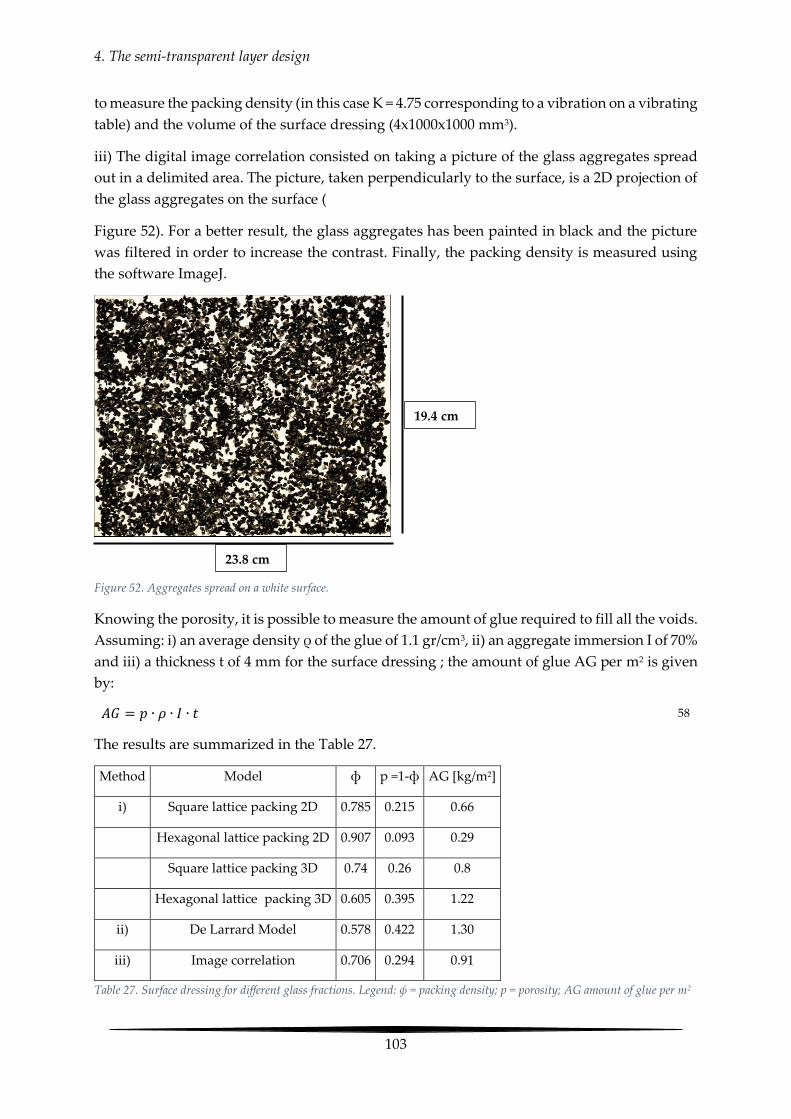
4. The semi-transparent layer design
103
to measure the packing density (in this case K = 4.75 corresponding to a vibration on a vibrating
table) and the volume of the surface dressing (4x1000x1000 mm3).
iii) The digital image correlation consisted on taking a picture of the glass aggregates spread
out in a delimited area. The picture, taken perpendicularly to the surface, is a 2D projection of
the glass aggregates on the surface (
Figure 52). For a better result, the glass aggregates has been painted in black and the picture
was filtered in order to increase the contrast. Finally, the packing density is measured using
the software ImageJ.
Figure 52. Aggregates spread on a white surface.
Knowing the porosity, it is possible to measure the amount of glue required to fill all the voids.
Assuming: i) an average density ρ of the glue of 1.1 gr/cm3, ii) an aggregate immersion I of 70%
and iii) a thickness t of 4 mm for the surface dressing ; the amount of glue AG per m2 is given
by:
𝐴𝐺 = 𝑝 ∙ 𝜌 ∙ 𝐼 ∙ 𝑡 58
The results are summarized in the Table 27.
Table 27. Surface dressing for different glass fractions. Legend: ф = packing density; p = porosity; AG amount of glue per m2
Method Model ф p =1-ф AG [kg/m2]
i) Square lattice packing 2D 0.785 0.215 0.66
Hexagonal lattice packing 2D 0.907 0.093 0.29
Square lattice packing 3D 0.74 0.26 0.8
Hexagonal lattice packing 3D 0.605 0.395 1.22
ii) De Larrard Model 0.578 0.422 1.30
iii) Image correlation 0.706 0.294 0.91
23.8 cm
19.4 cm

4. The semi-transparent layer design
104
The circle packing models in 2D give the lowest quantities of glue. This appears logical as it
describes an ideal situation with perfectly round aggregates in only 2D.
The 3D packing models are giving higher glue volume due to the third dimension taken into
account.
De Larrard model is 3D as well and it gives the highest glue volume since the aggregates are
not considered as perfect spheres. It as to be noted that this model has been developed for
concrete and may not be applicable for casting in a very thin layer as it is the case here (4mm).
Finally, the image correlation, which is a 2D approach, appears as the most reliable one. This
method is appropriate for a very thin layer and consists of a direct measurement of the
aggregates porosity. The final solution appears coherent with the standard and it is given by
1.99 kg/m2 of glass aggregates 2/4mm uniformly spread on a thin layer of polyurethane (0.9
kg/m2).
4.7.2 Optical performance, toughness and skid resistance
The optical performance is evaluated studying the power loss of the solar cell because of the
surface dressing treatment. The procedure is the same one performed for the STL1 and STL2
(see chapter 4.4).
The power loss has been measured on four samples using the polyurethanes A, B, C and D
and with a surface dressing having 1.99 kg/m2 of glass aggregates 2/4mm and an amount of
glue of 0.9 kg/m2.
The polymerization of the binder was achieved after 24 hours, at the room temperature of
20 °C. The power loss of glue A is the highest (43.4%), probably because of the N-
formylmorpholine, a white solid catalyst which makes the glue less transparent. The power
loss (Table 28) of the glues B, C and D is lower and it is around 15%. The result is very
encouraging, considering that the best power loss of STL2 was around 43%.
The three-point bending test has not been performed for STL3. Nevertheless, the toughness of
the sample number 1 of Table 19 with 33.3 % of glue content and 0.6 cm of thickness could be
comparable with the toughness of the STL3, because of the high glue content and low
thickness. In particular, the toughness of the sample number 1 is 0.162 MPa, which is close to
the toughness of the asphat mixture BBSG (0.109 MPa).
In terms of skid resistance (Table 28), the British Pendulum has been performed on the same
samples in wet conditions, obtaining a BPN (British Pendulum Number) between 56 and 67.
The results, higher than 55, are “generally satisfactory, meeting all but the most difficult
conditions encountered on the roads” [156]. The big gap between the sample B and C is not
due to the type of polyurethane, but probably to the presence of some protruding aggregate.
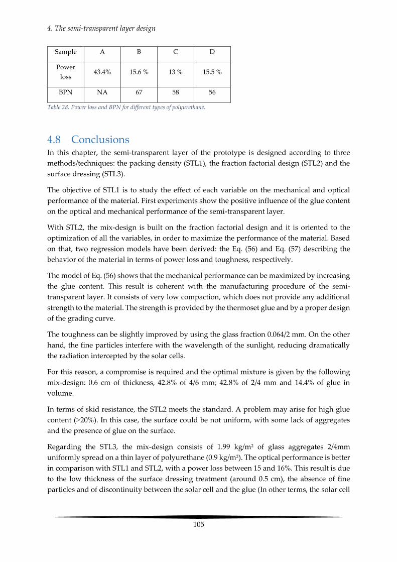
4. The semi-transparent layer design
105
Sample A B C D
Power
loss 43.4% 15.6 % 13 % 15.5 %
BPN NA 67 58 56
Table 28. Power loss and BPN for different types of polyurethane.
4.8 Conclusions In this chapter, the semi-transparent layer of the prototype is designed according to three
methods/techniques: the packing density (STL1), the fraction factorial design (STL2) and the
surface dressing (STL3).
The objective of STL1 is to study the effect of each variable on the mechanical and optical
performance of the material. First experiments show the positive influence of the glue content
on the optical and mechanical performance of the semi-transparent layer.
With STL2, the mix-design is built on the fraction factorial design and it is oriented to the
optimization of all the variables, in order to maximize the performance of the material. Based
on that, two regression models have been derived: the Eq. (56) and Eq. (57) describing the
behavior of the material in terms of power loss and toughness, respectively.
The model of Eq. (56) shows that the mechanical performance can be maximized by increasing
the glue content. This result is coherent with the manufacturing procedure of the semi-
transparent layer. It consists of very low compaction, which does not provide any additional
strength to the material. The strength is provided by the thermoset glue and by a proper design
of the grading curve.
The toughness can be slightly improved by using the glass fraction 0.064/2 mm. On the other
hand, the fine particles interfere with the wavelength of the sunlight, reducing dramatically
the radiation intercepted by the solar cells.
For this reason, a compromise is required and the optimal mixture is given by the following
mix-design: 0.6 cm of thickness, 42.8% of 4/6 mm; 42.8% of 2/4 mm and 14.4% of glue in
volume.
In terms of skid resistance, the STL2 meets the standard. A problem may arise for high glue
content (˃20%). In this case, the surface could be not uniform, with some lack of aggregates
and the presence of glue on the surface.
Regarding the STL3, the mix-design consists of 1.99 kg/m2 of glass aggregates 2/4mm
uniformly spread on a thin layer of polyurethane (0.9 kg/m2). The optical performance is better
in comparison with STL1 and STL2, with a power loss between 15 and 16%. This result is due
to the low thickness of the surface dressing treatment (around 0.5 cm), the absence of fine
particles and of discontinuity between the solar cell and the glue (In other terms, the solar cell

4. The semi-transparent layer design
106
is fully merged with the polyurethane). Moreover, the high glue content will insure the
mechanical strength.
Finally, STL3 seems to be the best solution, both for simplicity of manufacture procedure and
low power loss. A problem may arise for the high glue content, which could suffer aging
phenomena. The next chapter will also try to answer this question.
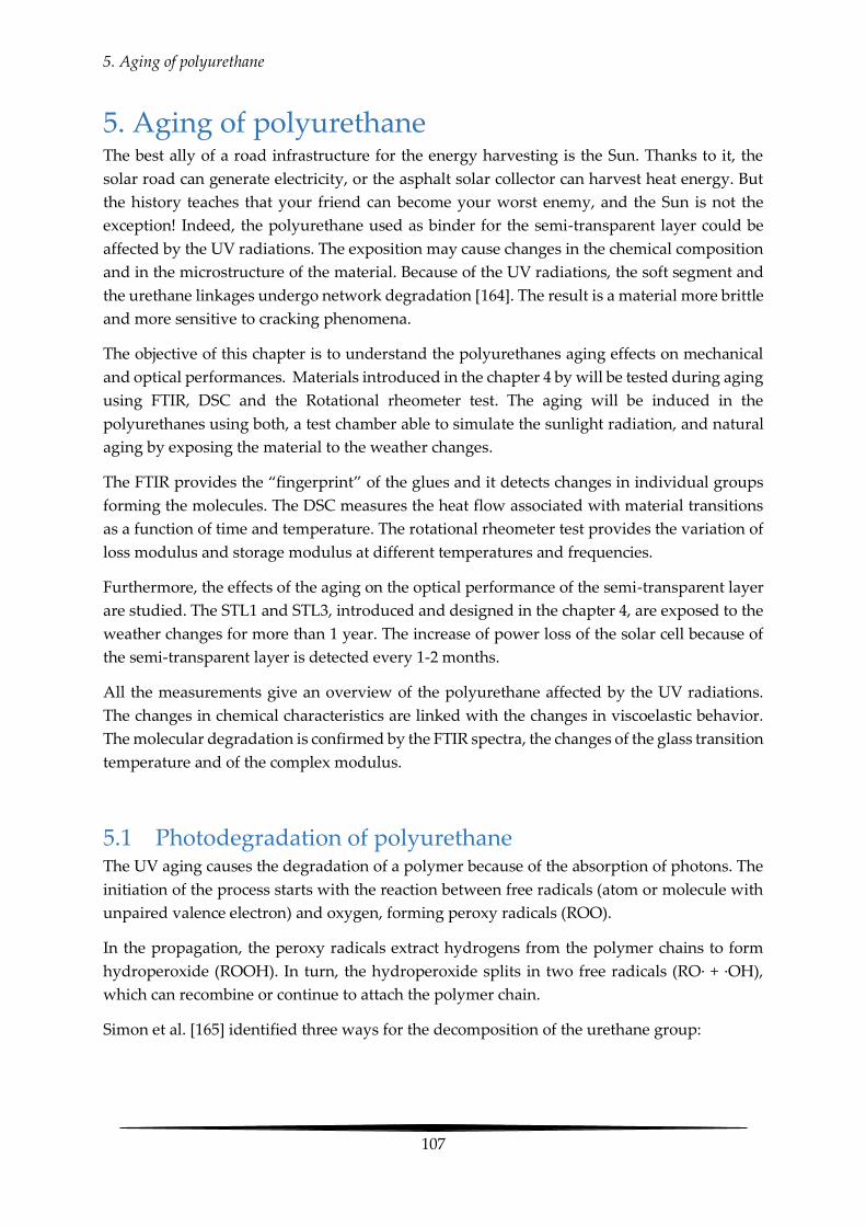
5. Aging of polyurethane
107
5. Aging of polyurethane The best ally of a road infrastructure for the energy harvesting is the Sun. Thanks to it, the
solar road can generate electricity, or the asphalt solar collector can harvest heat energy. But
the history teaches that your friend can become your worst enemy, and the Sun is not the
exception! Indeed, the polyurethane used as binder for the semi-transparent layer could be
affected by the UV radiations. The exposition may cause changes in the chemical composition
and in the microstructure of the material. Because of the UV radiations, the soft segment and
the urethane linkages undergo network degradation [164]. The result is a material more brittle
and more sensitive to cracking phenomena.
The objective of this chapter is to understand the polyurethanes aging effects on mechanical
and optical performances. Materials introduced in the chapter 4 by will be tested during aging
using FTIR, DSC and the Rotational rheometer test. The aging will be induced in the
polyurethanes using both, a test chamber able to simulate the sunlight radiation, and natural
aging by exposing the material to the weather changes.
The FTIR provides the “fingerprint” of the glues and it detects changes in individual groups
forming the molecules. The DSC measures the heat flow associated with material transitions
as a function of time and temperature. The rotational rheometer test provides the variation of
loss modulus and storage modulus at different temperatures and frequencies.
Furthermore, the effects of the aging on the optical performance of the semi-transparent layer
are studied. The STL1 and STL3, introduced and designed in the chapter 4, are exposed to the
weather changes for more than 1 year. The increase of power loss of the solar cell because of
the semi-transparent layer is detected every 1-2 months.
All the measurements give an overview of the polyurethane affected by the UV radiations.
The changes in chemical characteristics are linked with the changes in viscoelastic behavior.
The molecular degradation is confirmed by the FTIR spectra, the changes of the glass transition
temperature and of the complex modulus.
5.1 Photodegradation of polyurethane The UV aging causes the degradation of a polymer because of the absorption of photons. The
initiation of the process starts with the reaction between free radicals (atom or molecule with
unpaired valence electron) and oxygen, forming peroxy radicals (ROO).
In the propagation, the peroxy radicals extract hydrogens from the polymer chains to form
hydroperoxide (ROOH). In turn, the hydroperoxide splits in two free radicals (RO· + ·OH),
which can recombine or continue to attach the polymer chain.
Simon et al. [165] identified three ways for the decomposition of the urethane group:

5. Aging of polyurethane
108
i) dissociation to constituent:
ii) decomposition to primary amine, olefin and carbon dioxide:
iii) formation of secondary amine:
Based on Whilelm and Gardette [166], in the case of aliphatic poly-ether urethanes, the soft
segment is the most sensitive part for the photodegradation. In the case of
polytetramethyleneglycol, called PTMG, the photo oxidation leads to the formation of
hydroperoxide (Figure 53).
Figure 53. Formation of hydroperoxide.
The hydroperoxide, is photo thermally unstable and it decomposes to give formate17, ester18
and hemiacetal19.
Tcharkhtchi et al. [167] identify three steps during aging of polyurethane:
- 1st step: post-crosslinking due to the continuation of the polymerization process;
- 2st step: network degradation due to the chain scission. The material becomes more
flexible but less stiff;
- 3rd step: continuation of network degradation due to the chain scission. The material
becomes more brittle.
17 It is the anion of the formic acid, having formula HCOOH 18 It derives from an acid in which at least a hydroxyl group OH is replaced by an –O–alkyl group. The general
formula is RCOOR’ 19 It is given from the addition of alcohol to an aldehyde (the aldehyde is an organic compounds having a carbonyl
functional group, C=O, in which the carbon atom has two remaining bonds that may be occupied by hydrogen. If
at least one of these substituents is hydrogen, the compound is an aldehyde. If neither is hydrogen, the compound
is a ketone)

5. Aging of polyurethane
109
In the case of thermoplastic polyurethane, characterized by linear or branched molecular
structure, the aging lead to brittleness. On the contrary, in the case of the thermosets,
characterized by a crosslinked structure, the aging enhances the flexibility.
The aging effect can be detected by the FTIR analysis (see chapter 5.4), studying the picks
reduction or their shift along the x-axis. For example, the decrease of the pick at 3300 cm-1 and
at 1540 cm-1, due to the stretching and deformation vibration of NH group indicates a loss of
urethane structures. This is due to the decomposition of the urethane bond in a primary amine,
olefin and carbon dioxide [168].
The reduction of the band at 1220 cm-1, associated to the stretching vibration of C-O-C groups
of the polyol, is related to the photooxidation of ether soft segments [169].
This result is confirmed by He et al [170]. The authors studied the aliphatic polyurethane and
they observed that the absorption peaks of −𝑁𝐻 − 𝐶𝑂𝑂 −, 𝐶 = 𝑂, 𝐶 − 𝑁 and 𝐶 − 𝑂 gradually
decreased, which means that 𝐶 = 𝑁 and 𝐶 = 𝑂 bonds fractured.
Based on Che et al. [171], the picks reduction indicates the beginning of chain scission or the
disappearance of a certain group. For example, the pick at 1020-1100 cm-1 is a good indicator
for the cleavage of the C–O–C bond, while the reduction and the shift towards lower
wavenumber of the N–H group around 3300 cm-1 suggests the N–H bond cleavage and the
reduction in the degree of hydrogen bonding.
The FTIR spectrum interpretation is also useful for the study of the hydrogen bonding. The
hydrogen bond is formed between a proton donor and a proton acceptor. In polyurethanes,
the urethane linkages contain both: the proton donor, given by the NH group and the proton
acceptor, given by the carbonyl group C=O, or by the alkoxy oxygen ̶ O ̶ [172].
The degree of phase separation between hard and soft segment can be detected by the pick
shift of the carbonyl group (around 1733 and 1703 cm-1 for free and bonded carbonyl group,
respectively) [173]. The ratio between bonded and free carbonyl gives information regarding
the amount of hydrogen bonding.
The H-bonding causes microphase separation of the hard and soft domains, enhancing the
mechanical properties of the material. Furthermore, improved phase separation leads to
stronger hydrogen bonding in the hard segments [174].
5.2 Materials Each polyurethane is obtained by mixing together the components α and β according to the
mass fractions indicated by the producer (see chapter 3.1). The mixing time is of 2 minutes at
room temperature. Before the trigger of the polymerization, the glue is stored for 1 minute in
a vacuum chamber at low vacuum [760 – 25 Torr] in order to remove the air bubbles.
Immediately after, the glue is laid on special molds having for dimensions 40*15*3 mm3 and
then stored for 24 hours at the temperature of 20°C.

5. Aging of polyurethane
110
The polyurethane is also used as binder for the manufacture of the semi-transparent layer STL1
and STL3 (see chapter 4), which are exposed to the weather changes for more than 1 year.
Based on the observations and the results of the chapter 3, the glues can be grouped as shown
in Figure 54: glues A and B, which are thermoset polyurethanes obtained by the reaction of
aliphatic diisocyanate and polyol and glues C and D, which are polyaspartics, a special type
of polyurea given by the reaction of isocyanate and polyamine.
Figure 54. Comparison of generic polyurethane and polyurea [175].
5.3 Aging condition The aging was induced based on two approaches: natural and accelerated.
In the case of natural aging, the semi-transparent layers STL1 and STL3 (see chapter 4) have
been exposed to the weather changes for more than one year. The samples have been placed
on the roof of the laboratory, which has not shaded areas during the day.
For the accelerated aging, only the transparent glues have been conditioned. The idea was to
simulate the exposition to the sunlight in a controlled environment. At this scope, the
polyurethanes have been aged using the SUNTEST XXL+, a large xenon lamp weathering and
lightfastness test chamber able to generate the UV radiations and regulate the temperature
(Figure 55).
Figure 55. Right: natural aging; left: sunlight simulator

5. Aging of polyurethane
111
Assuming for the Central Europe weather an average irradiation of 215 MJ/m2 per year [176]
and generating a sunlight radiation of 60W/m2, the time of exposition in the device to simulate
1 year of sunlight is around 41 days (Figure 56).
In order to track the evolution of the material’s properties, the samples have been grouped at
different times of exposition into the SUNTEST: t0 corresponds to no aging; t1 corresponds to
4 months of natural UV exposition; t2 corresponds to 8 months and t3 corresponds to 12
months.
The aging has been performed at 60°C, which is a realistic temperature for a road pavement.
5.4 FTIR: Fourier transformer infrared spectroscopy The IR spectroscopy detects the interaction of light with the atoms and molecules of the sample
under investigation. The incident IR light can be absorbed by the oscillation arising from the
vibration and rotation of molecules. In general, most of the energy needed to excite organic
molecules falls in the spectral wavenumber region between 4000 cm-1 and 250 cm-l [177].
The incident light is absorbed by various parts of molecules, which are vibrating with a
particular frequency at room temperature. The absorption of this energy increases the
frequency of vibration.
Individual groups vibrate at different frequencies depending upon the strength of the bond
between the constituent atoms, their masses and the type of vibration occurring.
Higher energy transitions are stimulated by higher frequencies (high wavenumber) photons
and vice versa, hence it is possible to identify the groups present by measuring the frequencies
of the light absorbed. Similar functional groups executing similar modes of vibration absorb
in very similar regions of the spectrum.
The most common technique of FTIR analysis are the transmission mode, in which the IR light
passes directly through the sample and the ATR (Attenuated Total Reflection) mode, in which
the IR light passes through a crystal before to interact with the sample [178] (Figure 57). The
ATR is also the technique used for this study.
t0 t1= 4 months t2=8 months t3 = 12months
Natural Aging Aging in real condition of exposition to the weather changes
t0 t1=13.6 days t2= 27.2 days t3 = 41 days
Accelerated Aging
Figure 56. Equivalence between natural and accelerated aging.

5. Aging of polyurethane
112
The working principle of the ATR-FTIR is based on the total internal reflection. When the IR
light hits the crystal, the light beam is reflected. If the angle of incidence is above the critical
angle θc of the crystal, all the light is internally reflected. This is the total internal reflection,
which is applied in the optical fiber to transmit the light along the cables.
Taking into account that the crystal (having a refractive index of n1) is in contact with the
sample (having refractive index of n2), a small fraction of the light extends into the sample as
an evanescent electric field.
Figure 57. Transmission mode vs ATR mode [179]. Legend: I0 = incident radiation; I = transmitted/reflected radiation; θ angle
of incidence of the radiation; n1 = refractive index of the crystal; n2= refractive index of the sample.
Based on the sample composition, part of the light is absorbed and the evanescent electric field
will be attenuated. Consequently, not all the light beam is reflected, resulting in attenuated
total reflection (ATR).
The amplitude of the electric field at the interface crystal-sample decreases exponentially with
the distance from the interface according to the formula:
𝐸 = 𝐸0𝑒−𝑧/𝑑𝑝 59
Where:
- E0 (V/m) is the electric field at the interface crystal-sample;
- z (μm) is the distance in which the electric field is measured;
- dp (μm) is the penetration depth and it represents the required distance to reduce the
electric field of e-1 and it is given by the formula:
𝑑𝑝 =𝜆
2𝜋𝑛1√𝑠𝑖𝑛2(𝜃) − (
𝑛2𝑛1)2 60
In particular:
- λ (μm) is the wavelength of incident light in vacuum;
- n1 (dimensionless) is the refractive index of the crystal;
- n2 (dimensionless) is the refractive index of the sample;
- θ ( °) is the angle of incidence.
The crystal used during the FTIR analysis was diamond, having n1=2.41 and θ=40° [179], while
the refractive index n2 of the polyurethane is around 1.5 [180].
In general, dp gives an estimation of the portion of sample which actually contributes to the
FTIR spectrum. In the case of polyurethane, the dp ranges between 1 and 10 μm (Figure 58) in
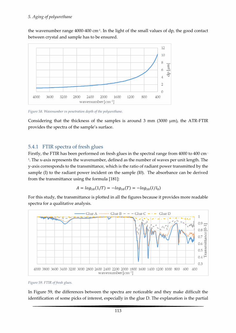
5. Aging of polyurethane
113
the wavenumber range 4000-400 cm-1. In the light of the small values of dp, the good contact
between crystal and sample has to be ensured.
Figure 58. Wavenumber vs penetration depth of the polyurethane.
Considering that the thickness of the samples is around 3 mm (3000 μm), the ATR-FTIR
provides the spectra of the sample’s surface.
5.4.1 FTIR spectra of fresh glues
Firstly, the FTIR has been performed on fresh glues in the spectral range from 4000 to 400 cm -
1. The x-axis represents the wavenumber, defined as the number of waves per unit length. The
y-axis corresponds to the transmittance, which is the ratio of radiant power transmitted by the
sample (I) to the radiant power incident on the sample (I0). The absorbance can be derived
from the transmittance using the formula [181]:
𝐴 = 𝑙𝑜𝑔10(1/𝑇) = −𝑙𝑜𝑔10(𝑇) = −𝑙𝑜𝑔10(𝐼/𝐼0)
For this study, the transmittance is plotted in all the figures because it provides more readable
spectra for a qualitative analysis.
Figure 59. FTIR of fresh glues.
In Figure 59, the differences between the spectra are noticeable and they make difficult the
identification of some picks of interest, especially in the glue D. The explanation is the partial

5. Aging of polyurethane
114
contact between the crystal of the ATR-FTIR and the sample, due to the stiffness of the glue.
The FTIR is performed at the room temperature of 20°C, for which the glue D is in glassy state.
In the light of above, the spectra analysis is qualitative and it is limited to the identification of
certain picks or any shifts, without taking into account variations of transmittance.
For a better interpretation, the plots have been split in two: the ranges 4000 - 2000 cm-1 (Figure
60) and 2000 – 400 cm-1 (Figure 61). For each range, the spectra have been normalized according
to the formula:
𝑦𝑛𝑜𝑟𝑚 =𝑦 − 𝑦𝑚𝑖𝑛
𝑦𝑀𝐴𝑋 − 𝑦𝑚𝑖𝑛 61
Where:
- ynorm is the value of transmittance which is normalized ;
- y is the transmittance ;
- ymin is the minimum value of transmittance ;
- yMAX is the maximum.
Figure 60. Normalized FTIR spectra of fresh glues in the range 4000-2000 cm-1.
Figure 61. Normalized FTIR spectra of fresh glues in the range 2000-400 cm-1.
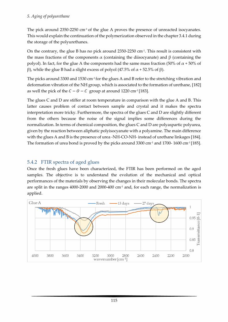
5. Aging of polyurethane
115
The pick around 2350-2250 cm-1 of the glue A proves the presence of unreacted isocyanates.
This would explain the continuation of the polymerization observed in the chapter 3.4.1 during
the storage of the polyurethanes.
On the contrary, the glue B has no pick around 2350-2250 cm-1. This result is consistent with
the mass fractions of the components α (containing the diisocyanate) and β (containing the
polyol). In fact, for the glue A the components had the same mass fraction (50% of α + 50% of
β), while the glue B had a slight excess of polyol (47.5% of α + 52.5% of β).
The picks around 3300 and 1530 cm-1 for the glues A and B refer to the stretching vibration and
deformation vibration of the NH group, which is associated to the formation of urethane, [182]
as well the pick of the 𝐶 − 𝑂 − 𝐶 group at around 1220 cm-1 [183].
The glues C and D are stiffer at room temperature in comparison with the glue A and B. This
latter causes problem of contact between sample and crystal and it makes the spectra
interpretation more tricky. Furthermore, the spectra of the glues C and D are slightly different
from the others because the noise of the signal implies some differences during the
normalization. In terms of chemical composition, the glues C and D are polyaspartic polyurea,
given by the reaction between aliphatic polyisocyanate with a polyamine. The main difference
with the glues A and B is the presence of urea -NH-CO-NH- instead of urethane linkages [184].
The formation of urea bond is proved by the picks around 3300 cm-1 and 1700- 1600 cm-1 [185].
5.4.2 FTIR spectra of aged glues
Once the fresh glues have been characterized, the FTIR has been performed on the aged
samples. The objective is to understand the evolution of the mechanical and optical
performances of the materials by observing the changes in their molecular bonds. The spectra
are split in the ranges 4000-2000 and 2000-400 cm-1 and, for each range, the normalization is
applied.

5. Aging of polyurethane
116
Figure 62. FTIR spectra of glue A after aging in the range 2000-4000 cm-1.
Figure 63. FTIR spectra of glue A after aging in the range 2000-400 cm-1.
Figure 62 and Figure 63 refer to the spectra of glue A subjected at different times of UV
exposition. After 13 days the photo degradation is not prominent. The difference is the
disappearance of the pick around 2350-2250 cm-1, associated with the unreacted isocyanate. It
proves that the polymerization process is completed. Furthermore, the pick around 3300 cm-1,
due to the stretching vibration of NH group, slightly increases and shifts towards lower

5. Aging of polyurethane
117
wavenumbers. It proves the increase of urethane linkages because the polymerization is finally
completed.
After 27 days, the changes are more relevant. In the not-normalized plot, the changes of
intensities in some picks (i.e. at 3300 cm-1 and at 1540 cm-1 due to the stretching and
deformation vibration of NH group) could be due to loss of urethane structure, or to the lack
of contact between the ATR-FTIR and the crystal during the analysis. Anyhow, the changes of
the band at 1220 cm-1, associated to the stretching vibration of C-O-C groups of the polyol, are
related to the photooxidation of ether soft segments.
The observations reported for the glue A are valid also for the glue B (see Annex 7).
Figure 64. FTIR spectra of glue C after aging in the range 4000-2000 cm-1.

5. Aging of polyurethane
118
Figure 65. FTIR spectra of glue C after aging in the range 2000-600 cm-1.
The spectra of glue C are less readable and they show more interferences, especially in the
wavenumber ranges 4000-2000 cm-1 (Figure 64 and Figure 65). The interference seems to
increase with the aging. An explanation could be that the material tends to be stiffer, affecting
the contact between the crystal of the ATR-FTIR and the sample. The picks of interest are
around 3300 and 1600-1700 cm-1 and they are related to the urea bonds. Under the hypothesis
that the not-normalized spectrum is realistic, the glue C undergoes major changes during the
first 13 days. The same observations can reported also for the glue D, whose spectra present
even more interferences (see Annex 8).
5.5 DSC: Differential scanning calorimetric test The DSC measures the response of the material to heating in terms of heat flow, defined as the
amount of heat supplied per unit time.
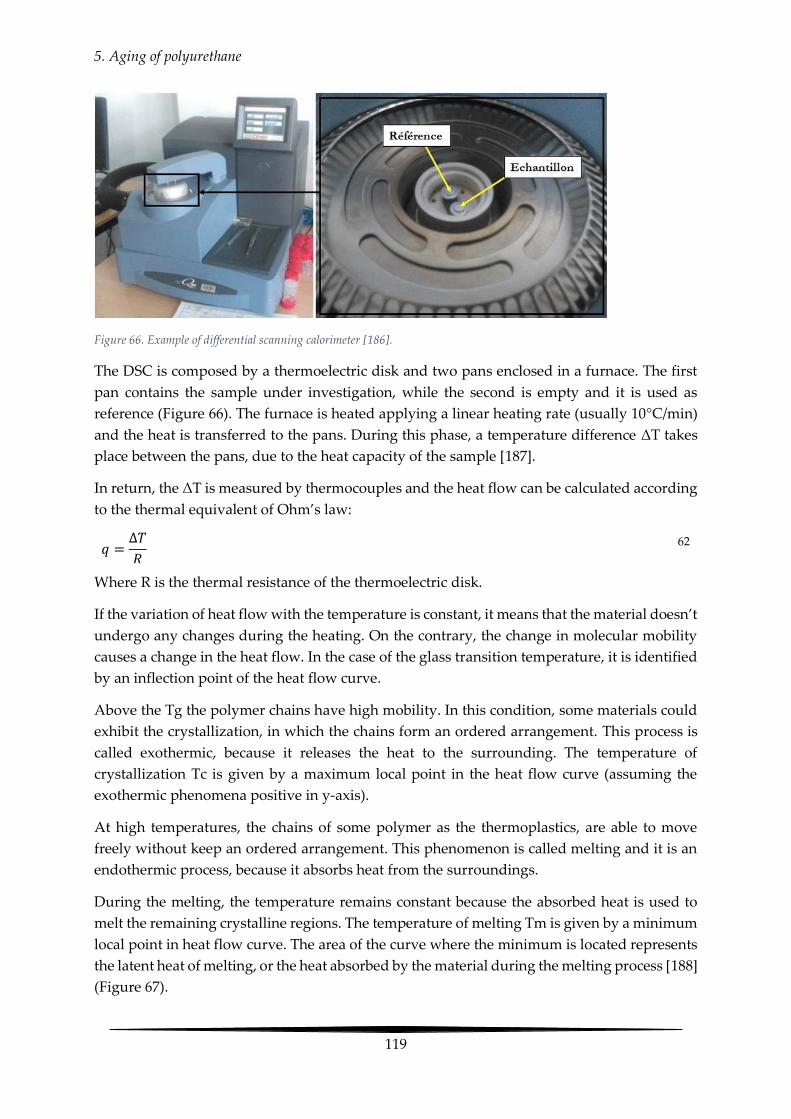
5. Aging of polyurethane
119
Figure 66. Example of differential scanning calorimeter [186].
The DSC is composed by a thermoelectric disk and two pans enclosed in a furnace. The first
pan contains the sample under investigation, while the second is empty and it is used as
reference (Figure 66). The furnace is heated applying a linear heating rate (usually 10°C/min)
and the heat is transferred to the pans. During this phase, a temperature difference ΔT takes
place between the pans, due to the heat capacity of the sample [187].
In return, the ΔT is measured by thermocouples and the heat flow can be calculated according
to the thermal equivalent of Ohm’s law:
𝑞 =∆𝑇
𝑅
62
Where R is the thermal resistance of the thermoelectric disk.
If the variation of heat flow with the temperature is constant, it means that the material doesn’t
undergo any changes during the heating. On the contrary, the change in molecular mobility
causes a change in the heat flow. In the case of the glass transition temperature, it is identified
by an inflection point of the heat flow curve.
Above the Tg the polymer chains have high mobility. In this condition, some materials could
exhibit the crystallization, in which the chains form an ordered arrangement. This process is
called exothermic, because it releases the heat to the surrounding. The temperature of
crystallization Tc is given by a maximum local point in the heat flow curve (assuming the
exothermic phenomena positive in y-axis).
At high temperatures, the chains of some polymer as the thermoplastics, are able to move
freely without keep an ordered arrangement. This phenomenon is called melting and it is an
endothermic process, because it absorbs heat from the surroundings.
During the melting, the temperature remains constant because the absorbed heat is used to
melt the remaining crystalline regions. The temperature of melting Tm is given by a minimum
local point in heat flow curve. The area of the curve where the minimum is located represents
the latent heat of melting, or the heat absorbed by the material during the melting process [188]
(Figure 67).
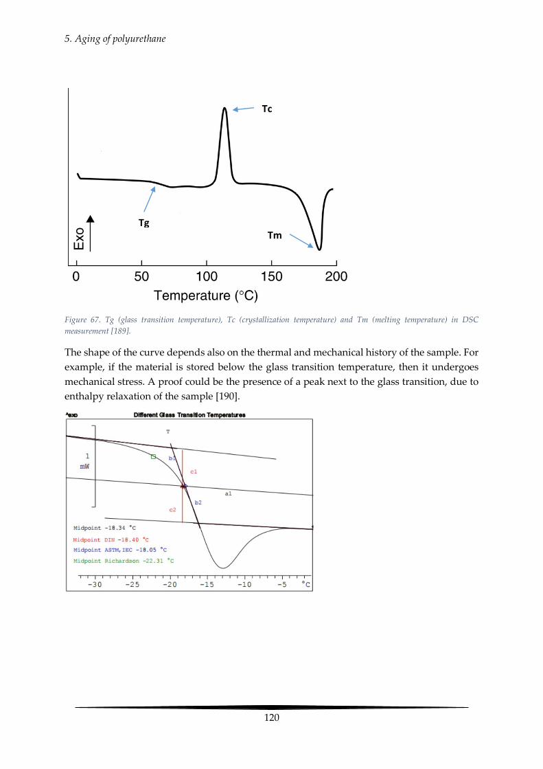
5. Aging of polyurethane
120
Figure 67. Tg (glass transition temperature), Tc (crystallization temperature) and Tm (melting temperature) in DSC
measurement [189].
The shape of the curve depends also on the thermal and mechanical history of the sample. For
example, if the material is stored below the glass transition temperature, then it undergoes
mechanical stress. A proof could be the presence of a peak next to the glass transition, due to
enthalpy relaxation of the sample [190].
Tg
Tc
Tm

5. Aging of polyurethane
121
Figure 68. Different methods to calculate the Tg [191].
The glass transition temperature can be calculated according to four methods (Figure 68): i)
the STARe, ii) the DIN, iii) the ASTM and iv) the Richardson method [191].
i) The STARe consists in drawing the bisector between the tangent below and above
the Tg. The intersection between the bisector and the heat flow curve gives the Tg;
ii) The DIN is the temperature to which the segments c1 and c2 are equidistant from
the tangents;
iii) In ASTM, the tangent is drawn at the inflection point of the heat flow curve. The
Tg is given by the midpoint of the onset and endset of the tangent;
iv) The Richardson method consists in drawing the tangent below and above the Tg.
The intersections between the tangents and the heat flow curve split up the plot in
three areas: A1, A2 and A3. The Tg is given by the highest temperature of A1, in
the condition that A2 = A1 + A3.
5.5.1 Aging effect on the glass transition temperature detected by means of
the DSC
The objective is to study the changing of the glass transition temperature Tg because of the
aging. The DSC has been performed on samples of mass between 5 and 10 mg, placed in
hermetic aluminum capsules. The procedure consists of cooling down the temperature of the
samples at -80°C, maintain it for 10 minutes and apply a temperature rate of 10°C/min until
rich 140 °C. The DSC provides the variation of heat flow with the temperature and the glass
transition temperature is given by the inflection point of the curve, based on the ASTM E1356
– 08 [192].
The changing of the Tg for each polyurethane are summarized in Table 29 and Figure 69:

5. Aging of polyurethane
122
Tg (°C)
A B C D
Unaged 11.8 8.6 53.8 28.8
Aged (13 days) 11.0 15.6 25.4 29.3
Aged (27 days) 19.2 20.3 29.9 31.4
Aged (41 days) 21.3 18.3 32.4 40.3
Table 29. Evolution of Tg because of aging, detected by the DSC.
Figure 69. Days of UV exposition vs Tg detected by the DSC.
The Tg is usually attributed to the motion of the soft-segment molecules [154]. At unaged
condition, the glues A and B have a lower value of Tg (around 10), while C and D have a higher
one. In general, Tg of soft segment increases with hard segment content [193].
The Tg of the unaged glue A is higher in comparison with glue B. This is consistent with the
measurements of the chapter 3.4.4. In fact, the part α (containing the hard segment) of glue A
represents 50% in mass, while for the glue B it is 47.5%.
The glues A, B and D show an increase of the Tg during the first 13 days of exposition to the
UV radiations. It can be attributed to post-cross linking phenomena and loss of volatile like
solvents.
The glue C, after 13 days of aging, shows a reduction of Tg, probably due to the residual stress
during cure. Immediately after the polymerization, occurred at 20°C (below the Tg), the
molecules are not totally relaxed in their equilibrium state. The crosslink network represents
a topological constraint. As consequence, the polyurethane is not able to relax stresses. During
the UV exposition, occurred close to the Tg, the molecular mobility increases and the material
tends to release the residual stress. Farzaneh et al. [194] observed a similar reduction of Tg

5. Aging of polyurethane
123
after recovery test for a polyurethane made of diphenylmethane diisocyanate (MDI) and a
polyester polyol.
Between 13 and 41 days, the Tg increases for all the glues. This result is due to the 1st step of
degradation of the polyurethane, which led to the formation of crosslink network and to the
restriction of the polymer chains mobility [195].
Figure 70. DSC curves measured at different aging time for the glue A.
The glue A at unaged state shows a melting temperature Tm at 64.2 °C. It means that not all
the diisocyanates reacted and they undergo melting (Figure 70). The melting disappears once
the UV aging is at 13 days.
Comparing the Tg of the fresh glues with that one measured by means of the DMA in chapter
3, the measurements have the same order of magnitude. The difference is due to the frequency-
dependence of the measurement performed by means of the DMA.
5.6 Rotational rheometer test: Linear domain determination The objective is to study the viscoelastic behavior of the polyurethanes, at different aging
times. The test has been performed in torsion mode on rectangle samples having for
dimensions 40*10*3 mm3. The sample is tightened between two clamps and the resulting span
ranges between 25 and 30 mm.
Firstly, the linear viscoelastic region (LVE) of the materials is detected. The LVE is defined as
the range in which the test can be carried out without destroying the structure of the samples.
At this scope, a logarithmic strain sweep has been performed at the temperatures of -20 and
60°C for a frequency of 1 Hz, in a range of strain between 10-3 % and 0.2%. The test provides
the variation of storage modulus G’ and loss modulus G’’ according to the strain percentage.
The procedure is shown in Figure 71.
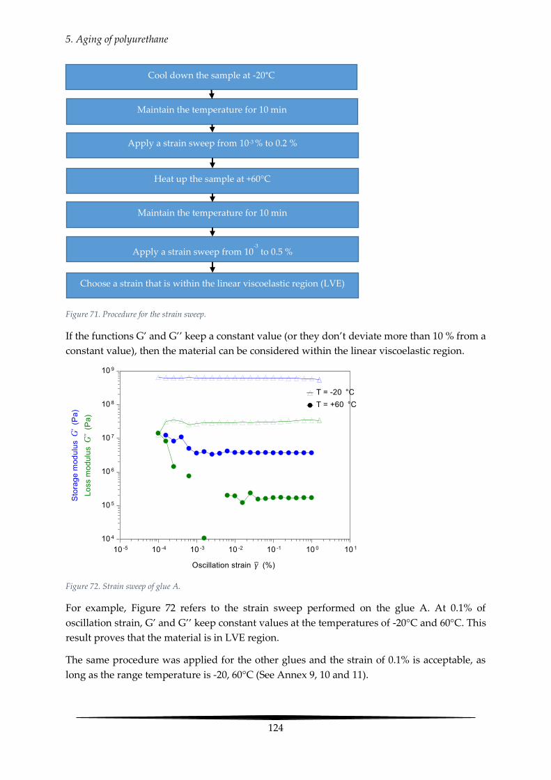
5. Aging of polyurethane
124
Figure 71. Procedure for the strain sweep.
If the functions G’ and G’’ keep a constant value (or they don’t deviate more than 10 % from a
constant value), then the material can be considered within the linear viscoelastic region.
Figure 72. Strain sweep of glue A.
For example, Figure 72 refers to the strain sweep performed on the glue A. At 0.1% of
oscillation strain, G’ and G’’ keep constant values at the temperatures of -20°C and 60°C. This
result proves that the material is in LVE region.
The same procedure was applied for the other glues and the strain of 0.1% is acceptable, as
long as the range temperature is -20, 60°C (See Annex 9, 10 and 11).
Glue A(2) unaged strain sweep
Cool down the sample at -20°C
Maintain the temperature for 10 min
Apply a strain sweep from 10-3 % to 0.2 %
Heat up the sample at +60°C
Maintain the temperature for 10 min
Apply a strain sweep from 10-3 to 0.5 %
Choose a strain that is within the linear viscoelastic region (LVE)

5. Aging of polyurethane
125
5.7 Complex modulus measurements The frequency sweep has been performed in the range 0.1 – 100 rad/sec for the temperatures
of -10, 0, 10, … 60°C. The frequency sweep follows the procedure shown in Figure 73.
Figure 73. Procedure for the frequency sweep.
As expected, the 4 polyurethanes behave like thermoset polymer having high degree of
crosslinking and short network links. Below the Tg, the polyurethanes are in glassy state and
they show the consistent of a rigid and brittle solid, with G’ ˃ ˃ G’’20 (Figure 77). At Tg, G’’
tends to increase (Figure 78). It means that the lost deformation energy of the material
increases, indicating higher internal flexibility. Nevertheless, G’ is ˃ G’’ also for T ˃ Tg.
According to the same approach used in chapter 3.3.4, the Tg has been measured at the
frequency of 1 Hz, assuming that it corresponds to the maximum of tan(δ) = G’’/G’.
The experimental values of tan(δ) of Figure 74 refers to the glue A and they are fitted using
spline interpolation. The Tg have been calculated also for the other glues at different aging
time. The results are listed in Table 30.
20 The symbol >> means that G’ is much higher than G’’
Cool down the sample at -10°C
Apply a strain within the LVE (i.e. 0.1%)
Perform frequency sweep from 0.1 to 100 rad/s
Heat up the samples of 10 °C
Maintain the temperature for 10 min
Measure the viscoelastic parameters

5. Aging of polyurethane
126
Figure 74. tan(δ) vs Temperature at different aging time for the glue A.
Tg (°C)
A B C D
Unaged 30.1 28.2 > 60 > 60
Aged (13 days) 30.5 30.5 50.7 50.1
Aged (27 days) 34.4 34.3 > 60 > 60
Aged (41 days) 38 38.7 > 60 > 60
Table 30. Evolution of Tg because aging, detected by the rotational rheometer test at the frequency of 1Hz.
In comparison with the measurements performed in chapter 3.4.4, the Tg of fresh glues have
the same order of magnitude. As expected, the Tg of the polyurethanes A and B increases
according to the aging time. This result is due to the 1st step of degradation of the polyurethane,
observed in the chapter 5.5.1.
The measurements of Tg using the rheometer are frequency-dependent and they increase
according to the frequency. In the light of this, the Tg have been calculated also at the
frequency of 0.01 Hz (Table 31, Figure 75), because most of the results of the glues C and D are
not detectable at the frequency of 1 Hz.
Table 31. Evolution of Tg because aging, detected by the rotational rheometer test at the frequency of 0.01Hz.
Tg (°C)
A B C D
Unaged 19.6 15.5 > 60 49.8
Aged (13 days) 19.9 19.7 47.5 40.3
Aged (27 days) 22.2 21.3 48.9 48.5
Aged (41 days) 24.0 26.0 49.4 50.0
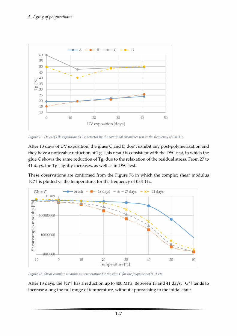
5. Aging of polyurethane
127
Figure 75. Days of UV exposition vs Tg detected by the rotational rheometer test at the frequency of 0.01Hz.
After 13 days of UV exposition, the glues C and D don’t exhibit any post-polymerization and
they have a noticeable reduction of Tg. This result is consistent with the DSC test, in which the
glue C shows the same reduction of Tg, due to the relaxation of the residual stress. From 27 to
41 days, the Tg slightly increases, as well as in DSC test.
These observations are confirmed from the Figure 76 in which the complex shear modulus
|G*| is plotted vs the temperature, for the frequency of 0.01 Hz.
Figure 76. Shear complex modulus vs temperature for the glue C for the frequency of 0.01 Hz.
After 13 days, the |G*| has a reduction up to 400 MPa. Between 13 and 41 days, |G*| tends to
increase along the full range of temperature, without approaching to the initial state.

5. Aging of polyurethane
128
The next plots refer to the frequency sweep of storage modulus G’ and loss modulus G’’, at
given temperature.
Figure 77. Frequency sweep of the glue A at - 10°C, for different aging time.
At -10°C the values G’ and G’’ of all the glues are almost frequency-independent. Considering
the different time of UV exposition, the function G’’ undergoes a progressive reduction along
all the frequencies. This could be due to the degradation of the soft segment of the
polyurethane, which controls the ability of the material to dissipate energy.
Figure 78. Frequency sweep of the glue A at 20°C, for different aging time.

5. Aging of polyurethane
129
Figure 79. Frequency sweep of the glue A at 60°C, for different aging time.
At 20°C, G’ and G’’ tend to increase with the frequency. Based on Figure 78, the difference
between the functions G’ and G’’ is smaller in comparison to the Figure 77 because the test
have been performed close the glass transition temperature of the glue A. Instead at 60°C, G’
is constant according to the frequency, while G’’ increases (Figure 79). The plots of the others
glues are in Annexes 12, 13 and 14.
5.8 Discussion The FTIR, the DSC and the rotational rheometer test provide some new informations about
the chemical and the viscoelastic behavior of the glues and they confirm some observations
pointed out in the chapter 3.
Firstly, the presence of unreacted diisocyanates in glue A, responsible of the post-
polymerization process detected after 1 month of storage time is confirmed. The excess of
diisocyanate is confirmed by the FTIR, because of the pick around 2350-2250 cm-1 and by the
DSC, because of an endothermic phenomenon detected at 64.2 °C, associated with the melting
of the diisocyanate.
The glue B has a similar behavior in comparison with glue A. The difference is a less
crosslinked structure, confirmed by lower values of Tg.
Glue A and glue B seem to undergo the aging in the same way: the UV irradiation leads to the
formation of a crosslinked structure on the exposed surface, which decreases the molecular
mobility. The result is a material slightly stiffer.

5. Aging of polyurethane
130
According to Tcharkhtchi et al [167], at the first stage of aging, the effect of cross-linking
overshadows the chain scission. In other terms, even if the chain scissions are taking place,
they are still few extended.
The glues C and D exhibit a reduction of Tg after 13 days of aging. This phenomenon could be
is due to the relaxation of residual stress, accumulated during the polymerization at
temperature below the Tg. From 13 to 41 days of UV exposition, the Tg tends to increase
because of the 1st step of degradation of the polyurethane, which lead to formation of crosslink
network and to the restriction of the polymer chains mobility.
5.9 Aging of the semi-transparent layer The optical performance of the semi-transparent layer is mostly affected by the aging of the
binder because of the exposition to the weather changes. According to Rosu et al. [197], the
polyurethanes made with an aromatic isocyanate become yellow because of the exposition to
UV light. The yellowing is due to the oxidation reaction in the backbone of the polymer.
In this study, the polyurethanes are composed by aliphatic diioscyanates, which make the
glues less reactive, but more resistant to yellowing.
Nevertheless, the aging has an impact on the material, causing transparency reduction, which
is indirectly measured monitoring the evolution of the power loss (see chapter 4.4) of the solar
cells, covered by the semi-transparent layer.
Based on Lee et al [198], the loss of transparency could be due to the crystallinities in the hard
segment. This latter leads to crystalline formation, which cause light scattering and
transparency reduction
For STL1, the manufactured samples have quadratic shape (15*15*1 cm3) and they are made of
glass aggregates and polyurethane, according to the following mix design in volume: i) 4/6mm
= 57%; ii) 2/4 mm = 38%; glue content = 5%. The variable in the mix-design is the type of glue:
A, B, C or D.
The STL1 doesn’t stick on the solar cell. Thanks to this, the intensity-voltage curve of the solar
cell can be derived before each test.
To guarantee an accurate measurement of the power loss, the radiation of the lamp has to be
constant during the test. For this reason, the irradiance is checked by means of a pyranometer.
Figure 80 shows the evolution of the power loss during 14 months.

5. Aging of polyurethane
131
Figure 80. Evolution of the power loss of STL1.
At time 0, the power loss ranges between 64 and 68% and it greatly increases after one month
of exposition for all the polyurethanes (probably because of the massive sunlight radiation in
July, which accelerates the aging phenomena of the glue). After 7 months, the aging looks to
stabilize for all the polyurethanes in a power loss range between 84 and 88%.
For a better comparison, the measurements are evaluated calculating the difference between
the power loss after 14 months and the power loss at time zero:
𝑃𝐿𝑑𝑖𝑓𝑓 = 𝑃𝐿𝑡14 − 𝑃𝐿𝑡0 where:
PLt0 is the initial power loss [%] and PLt14 is the power loss after 14 months [%].
The results are summarized in the table below:
Glue PLdiff
A 17.9%
B 18.5%
C 15.8%
D 14.8%
Table 32. Power loss difference between time 14 and time 0 for STL1.
Based on the results of Table 32, the glue C and D are the less affected by aging.
The evolution of power loss has been monitored also for STL3 (Figure 81). The main difference
is the amount of glue: in STL1 is around 5%, while in STL3 is pure glue. More in detail, the
mix-design of STL3 consists of 1.99 kg/m2 of glass aggregates 2/4mm uniformly spread on a
thin layer of binder (0.9 kg/m2). Unlike the STL1, the solar cell is imbedded into the glue. This
means that the intensity-voltage curve of the solar cell is measured only one time before to
imbed the solar cell.
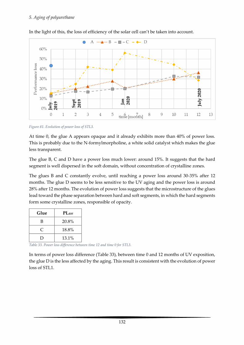
5. Aging of polyurethane
132
In the light of this, the loss of efficiency of the solar cell can’t be taken into account.
Figure 81. Evolution of power loss of STL3.
At time 0, the glue A appears opaque and it already exhibits more than 40% of power loss.
This is probably due to the N-formylmorpholine, a white solid catalyst which makes the glue
less transparent.
The glue B, C and D have a power loss much lower: around 15%. It suggests that the hard
segment is well dispersed in the soft domain, without concentration of crystalline zones.
The glues B and C constantly evolve, until reaching a power loss around 30-35% after 12
months. The glue D seems to be less sensitive to the UV aging and the power loss is around
28% after 12 months. The evolution of power loss suggests that the microstructure of the glues
lead toward the phase separation between hard and soft segments, in which the hard segments
form some crystalline zones, responsible of opacity.
Glue PLdiff
B 20.8%
C 18.8%
D 13.1%
Table 33. Power loss difference between time 12 and time 0 for STL3.
In terms of power loss difference (Table 33), between time 0 and 12 months of UV exposition,
the glue D is the less affected by the aging. This result is consistent with the evolution of power
loss of STL1.

5. Aging of polyurethane
133
5.10 Conclusions This chapter points out the effect of the UV radiation on the chemical and viscoelastic behavior
of the polyurethanes. In the purpose of a full characterization, an experimental campaign is
conducted performing the FTIR, the DSC and the rotational rheometer test.
Due to the poor quality of the spectra obtained by FTIR, the analysis is qualitative and it
focuses on the detection of picks that prove the presence of certain bonds, or any shifts along
the wavenumbers.
The DSC provides the glass transition temperature of the materials at different times of UV
exposition. After 41 days, the glue C undergoes slower changes in Tg, as confirmed also by the
measurements of Tg using the rotational rheometer test.
For this type of glues, the UV aging within the 41 days causes post-polymerization and the
reduction of transparency could be due to the phase separation between hard and soft
segments, leading the formation of crystalline zones. However, there is no evidence of link
between the reduction of transparency and the results of the FTIR, DSC and DSR.
In terms of power loss, the STL3 guarantees the best performance in comparison to STL1.
Among the glues, the glue D seems to be the less affected by natural aging, followed by the
glue C.
In the light of this, both glues are good candidates as binder for a solar road. The choice
depends on the operating temperature of the pavement. The ideal would be to operate close
to the glass transition temperature. In this condition, the dissipative behavior of the glues is
enhanced and it could lead to a greater fatigue resistance and less cracking phenomena.

General conclusions
135
General conclusions Energy harvesting is the process by which energy is captured exploiting an external source
(e.g., solar power, thermal energy, wind energy, electromagnetic ambient energy, kinetic
energy, etc.).
Every day, the road network is exposed to a big amount of sunlight, up to 40MJ/m2 in summer.
If this amount of energy could be effectively used, it would mark a revolution. Furthermore,
the use of existing transportation infrastructures for energy harvesting may avoid to occupy
new lands, which could be exploited for other purposes (agriculture, industry etc.) or to
preserve the biodiversity in some special areas.
The sunlight radiation can be directly converted into electricity thanks to solar cells placed
under a semi-transparent layer (photovoltaic road), or it can be harvested by means of a heat-
transfer fluid (thermal solar systems). At present, the traditional way consists of a pipe
network imbedded into the asphalt, in which the water is able to extract heat energy, due to
the gradient temperature between the fluid and the asphalt. Based on recent researches, the
pipes network can be replaced by a porous layer, which operates as an active solar collector.
For these technologies, the semi-transparent layer plays a fundamental role because it has to
support the traffic load, guarantee the friction, protect the solar cells and, at the same time,
allow the passage of the sunlight and maximize the heat transfer to the lower layers.
In the light of the above, the core of the thesis focuses on the design of the top layer and on a
comprehensive characterization of the polyurethane as binder.
Firstly, the state of the art of energy harvesting through road infrastructure is extensively
studied. With surprise, there is a debated and lively research in academia and industry, with
appreciable in situ applications of working prototypes. For better-understanding potentials
and limits, the different technologies are compared in terms of initial cost, technology
readiness level, efficiency and electrical output. From this analysis, the solar road and the
asphalt solar collectors seem the most promising, notwithstanding the initial cost still too high
and the low efficiency of the related technologies (i.e. the solar cells for the solar road and the
piezoelectric material for the piezoelectric road).
The review of the state of art aims to identify some critical issues that could affect the
performance of the solar roads and of the porous layers as solar thermal systems. The
following main criticisms can be listed:
i) In the early stage of the implementation, the power loss of the solar cells because of the
semi-transparent layer can reach more than 70%;
ii) The use of epoxy as binder in the top layer is not recommended because it is strongly
affected by aging, which causes premature yellowing and brittleness;
iii) The use of asphalt mixture as active solar collector doesn’t maximize the energy
harvesting, because of the low porosity of middle layer, which is around 20-23%.
Moving from these observations, it is proposed to replace epoxy by polyurethane.
General conclusions
136
For a better understanding of the manuscript, the literature review is enriched with an
introduction about the polyurethane. Based on the chemical composition (type of diisocyanate
and polyol, type of chain extender, presence of catalysts or solvents), the ratio between hard
and soft segments, the manufacturing process and the external conditions (temperature,
pressure, presence of UV radiations or oxygen), the polyurethane can be synthesized for many
applications in different fields. In the case of a solar road, it must meet the following specific
requirements:
i) transparency, in order to minimize the loss of solar radiations;
ii) strength, in order to support the traffic load;
iii) adhesion with the glass aggregates to avoid pull out;
iv) resistance to aging, because of the exposition to the weather changes;
v) withstand to a wide range temperature (-10 to 60°C);
vi) workability.
Based on that, the thermoset polyurethanes seem to be the best candidate.
The literature review continues with some introductory notions about the methods/techniques
applied for the mix design of the semi-transparent layer.
After that, the kinetic and viscoelastic characterization of the polyurethane is investigated. This
study focuses on four glues: two thermoset polyurethanes (A and B) obtained by the reaction
of aliphatic diisocyanate and polyol and two polyaspartics (C and D), some special types of
polyureas given by the reaction of isocyanate and polyamine.
The first objective is to determine the curing time of the glue by means of the Dynamic Shear
Rheometer. At this scope, a special procedure is implemented, in which the applied stress of
DSR increases according to the glue consistency during the polymerization. The result of this
procedure is a plot composed in y-axis of shear complex modulus and phase angle and in x-
axis of the time. The curing time is detectable studying the trend of the shear complex modulus
with the time. Two behaviors are observable: in the first portion of the curve, |G*| increases
slowly, while in the second it increases more quickly. The curing time corresponds to the
intersection between the tangents to the two portions of the plot.
Applying this criterion, the curing time is measured for all the glues at the curing temperature
of 10, 30 and 50°C. As expected, it is strictly dependent on the curing temperature of the glue.
For example, at the temperature of 10°C, the curing time ranges between 30 and 60 hours,
while at 50°C it ranges between 1 and 3.5 hours. According to this, any outdoor applications
should be carried out during summer time, when the average temperature is higher.
The experimental values of curing time are modeled using the Arrhenius law, which depends
on two parameters: the pre-exponential factor Δ and the energy of activation E. This latter
quantifies the requested energy for the polymerization, which is 80445, 61566, 59274 and 49126
J/mol for the glue A, B, C and D. The different values are influenced by the presence of catalysts
(such as the dibutyltin dilaurate in the glue B), or by the nature of the chemical reaction, giving
urethane bonding for the glues A and B and urea for the glues C and D.

General conclusions
137
The viscoelastic behavior is studied performing the Dynamic Mechanical Analysis on solid
samples, at the curing temperature of 10, 30 and 50°C. A first comparison refers to the complex
modulus vs temperature, at the frequency of 1 Hz. All the glues behave like thermoset
polymers. At low temperatures (<0°C), they are in the glassy region, characterized by a
complex modulus higher than 1E+9 Pa. As the temperature increases (>0 °C), the modulus falls
through the glass transition region where the glues behave like a viscoelastic material and the
complex modulus is temperature dependent. At higher temperatures (>60°C), the
polyurethanes are in the rubbery plateau region and the complex modulus stabilizes. More in
detail, the complex modulus at 20°C (1Hz) gives the following ranking (by ascending order):
B < A < C < D, whatever the curing temperature. This result is mainly attributed to the
viscoelastic state of the glues, which are at 20°C, partly in the glassy state (glue C and D) and
partly in the rubbery state (glue A and B).
The overall behavior shows an increase of the stiffness when the curing temperature decreases.
An explanation could be that the solvents of the polyurethanes evaporate faster at higher
temperatures. In that situation, some isocyanates can get trapped in the polymer network and
they don’t react to form others urethane linkages, bringing to reduction of crosslinking density
and, consequently, of stiffness.
The viscoelastic behavior of the glues is modeled using generalized Maxwell. The model
provides the storage modulus E’ and the loss modulus E’’ at any frequency and temperature.
The ratio between E’’ and E’ gives the tangent of phase angle δ (tan(δ)=E’’/E’). In return, the
maximum of tan(δ) corresponds to the glass transition temperature Tg.
The Tg is function of the network structure and it increases according to the crosslink density
or the hard segment content. For example, the glue B, composed by long-chain molecules, has
low crosslinks density and the low Tg; vice-versa the glue C, which is a high-stiffness
polyaspartic, has high crosslinks density and the high Tg. Furthermore, the curing
temperature affects the Tg: the more is the curing temperature, the less is the Tg.
Once the kinetic and the viscoelastic behavior of the glues in unaged condition are well-
defined, the following step is the mix-design of the semi-transparent layer. This latter is a
composite material made of glass aggregates bonded together using the polyurethane as
binder. The mix-design is based on three methods/techniques: the particle packing degree
(Semi Transparent Layer 1, STL1), the fraction factorial design (STL2) and the surface dressing
(STL3).
Each proposal is characterized in terms of optical and mechanical performance. The optical
performance consists in evaluating the power loss of the solar cell because of the semi-
transparent layer, while the mechanical performance consists in measuring the toughness of
the material by means of the three-point bending test.
In STL1, the idea is to reduce the porosity of the medium and optimize the use of the glue, in
order to increase the strength of the material. The results highlight the positive effect of the
glue content on both optical and mechanical performance. More in detail, for a glue content
around 20 %, the toughness reaches the same order of magnitude of the asphalt mixture BBSG.

General conclusions
138
In STL2, the fraction factorial design is applied to derive two regression models describing the
behavior of the material in terms of power loss and toughness. The results are consistent with
SLT1, in fact the reduction of thickness and the increase of glue content are both positive for
the material performance. The discrepancy is due to the use of fine particles, which improve
the toughness, but they interfere with the sunlight wavelength, reducing dramatically the
radiation intercepted by the solar cells. Based on that, the optimal mixture is given by: 0.6 cm
of thickness, 42.8% of 4/6 mm; 42.8% of 2/4 mm and 14.4% of glue in volume.
In terms of skid resistance, the STL2 meets the standard. A problem may arise for high glue
content (˃20%). In this case, the surface could be not uniform, with some lack of aggregates
and the presence of glue on the surface.
Based on the results of STL1 and STL2, the optical and mechanical performance can be both
improved increasing the glue content. In the light of this, the STL3, inspired by the surface
dressing treatment, seems to be the best solution. The technique consists of laying down the
glass aggregates on a thin layer of glue. The aggregates have not to be totally immerged into
the glue, in order to provide skid resistance to the surface. The optimum glue content is given
by the amount of binder required to fill the voids and guarantee an immersion of the glass
aggregates of 70%. Based on the image correlation method, the mix-design for the STL3 is 1.99
kg/m2 of glass aggregates 2/4mm and 0.9 kg/m2 of glue. The optical performance appears better
in comparison with STL1 and STL2, with a power loss of the solar cells measured between 15
and 16%. This good result is due to the low thickness of the surface dressing treatment (around
0.5 cm), the absence of fine particles and of discontinuity between the solar cell and the glue.
The last step is to understand the aging of the glue. The UV exposition is induced by means of
a sunlight simulator, or exposing the semi-transparent layer to the weather changes. The
experimental campaign is conducted performing Fourier Transform Infrared Spectroscopy
test (FTIR), the Differential Scanning Calorimetry (DSC) and the rotational rheometer test. The
FTIR is in ATR (Attenuated Total Reflection) mode, in which the IR light passes through a
crystal before to interact with the sample. Because of the high stiffness of the glue, the quality
contact between crystal and sample is poor (especially for the glues C and D) and this affects
the spectra readability. In the light of this, the analysis remained qualitative and it is limited
to the identification of certain picks of interest or any shifts along the x-axis (wavenumber).
Observing the plots, the pick around 2270-2250 cm-1 of the glue A proves the presence of
unreacted isocyanates. The same pick disappears after 13 days of aging and it is not detected
in glue B. This is consistent with the composition of the glue B, which contains less diisocyante
in comparison with glue A.
The formation of urethane for glues A and B is proved by the picks around 3300 and 1530cm-
1, associated with the stretching vibration and deformation vibration of the NH group, and by
the pick at 1220 cm-1 , associated to the C-O-C group. For the glue C and D, the formation of
urea is proved by the picks around 3300 cm-1 and 1700- 1600 cm-1.
In terms of aging, Glue A and glue B seem to behave in the same way: the UV irradiation leads
to the formation of a crosslinked structure on the exposed surface, which decreases the

General conclusions
139
molecular mobility. The result is a material slightly stiffer. In this initial stage of aging, the
effect of cross-linking overshadows the chain scission and the stiffness of the glue increases.
This observation is consistent with the measurements of Tg, which increases according to the
time of UV exposition.
For the glue C and D, there are no evidences of post-polymerization. On the contrary, they
exhibit a reduction of Tg after 13 days of aging. This phenomenon could be due to the
relaxation of residual stress, accumulated during the polymerization at temperature below the
Tg. From 13 to 41 days of UV exposition, the Tg increases for all the glues. This result is due
to the 1st step of degradation of the polyurethane, which leds to the formation of crosslink
network and to the restriction of the polymer chains mobility.
The natural aging is induced in STL1 and STL3, with the objective of tracking the evolution of
power loss, due to the exposition to the weather changes. After 12 months, the power loss of
STL1 is around 82-86%, while for STL3 is around 30-35%. The increase of power loss suggests
that the microstructure of the glues leads toward the phase separation between hard and soft
segments, in which the hard segments form some crystalline zones, responsible of opacity.
For what concerns the glues, C and D are the less affected by natural aging. In the light of this,
both glues are good candidates as binder for a solar road. The final choice depends on the
operating temperature of the pavement in comparison to the glass transition temperature of
the glue.
Perspectives The viscoelastic characterization of the polyurethane and the mix-design of the semi-
transparent layer is an important step towards the manufacture of the “hybrid road”. This
latter is given by the union between a concrete porous medium with a photovoltaic road. The
“hybrid road” is a pavement able to generate electricity and, at the same time, harvest energy
by means of a heat-transfer fluid pumped in the porous layer.
The system is a sandwiched structure composed by four layers (see Annex 4):
i) a semi-transparent layer made of glass aggregates bonded together using a
polyurethane glue;
ii) an electrical layer containing the solar cells for the generation of electricity;
iii) a porous concrete layer for the circulation of a heat-transfer fluid, able to extract the
heat energy from the pavement;
iv) a waterproof base layer able to prevent the loss of the heat-transfer fluid.
The choice of the porous concrete is due the high permeability of this material, in comparison
with the porous asphalt mixture.
The natural continuation of this project is the mix-design of the porous layer, in which the heat
exchange between the water and the pavement takes place. Some preliminary measurements
have already been carried out, in order to identify an aggregate fraction with low packing

General conclusions
140
density and, consequently, high porosity. The objective is to maximize the permeability of the
porous layer and, potentially, increase the harvested energy.
Based on De Larrard model, the following mix-design is proposed: i) Cement CEM I 52.5 = 375
Kg/m3; ii) 10/14 Corse Aggregate – Gneiss: 1269 Kg/m3 and iii) water 84 Kg/m3.
Using a classical planetary mixer and applying a low manual compaction, a porous concrete
containing 34.4% of embedded air and presenting 5.3 cm/s of permeability was obtained. This
permeability is more than the double of the one obtained with a porous asphalt mixture
(around 2 cm/s).
For the base layer, which avoids the loss of the heat-transfer fluid, a solution could come from
the waterproofing layers techniques used in pavements on bridge decks.
Once the prototype is assembled, it can be evaluated in terms of harvested energy, bearing
capacity, load cycles and skid resistance. The harvested energy could be measured in lab
and/or real conditions, tracking the electrical output of the solar cells in reference to the
sunlight radiation or measuring the increase of the water temperature due to the heat exchange
with the pavement. The bearing capacity could be assessed in static or dynamic conditions,
simulating the heavy traffic and load cycles in order to evaluate the fatigue failure of the
pavement. Finally, skid resistance and harvested energy could be measured before and after
the load cycles, or tracked during a certain time interval.
Further researches could move towards the improvement of the system by using new
materials (i.e. novel transparent glues or aggregates), modeling the pavement using FEM
analysis or performing the life cycle assessment for calculating the environmental impact of
the “hybrid road”.
The comprehensive characterization of the prototype will be helpful moving from the
laboratory to the site, in the perspective of a full scale application.
Résumé long Chaque jour, le réseau routier est exposé à un ensoleillement important, jusqu'à 40MJ/m2 en
été. Si cette quantité d'énergie pouvait être utilisée efficacement, cela marquerait une
révolution. En outre, l'utilisation des infrastructures de transport existantes pour la
récupération d'énergie peut éviter d'occuper de nouvelles terres, qui pourraient être exploitées
à d'autres fins (agriculture, industrie, etc.) ou pour préserver la biodiversité dans certaines
zones particulières.
La récupération d'énergie au travers des infrastructures routières a été largement étudié. De
manière surprenante, de nombreuses recherches menées au sein des universités et de
l'industrie existent, avec des applications in situ convaincantes de prototypes fonctionnels.
Pour mieux comprendre leurs potentiels et leurs limites, ces différentes technologies ont été
comparées en termes de coût initial, de niveau de développement technologique, d'efficacité
et de puissance électrique. De cette analyse, la route solaire et système solaires thermiques

General conclusions
141
développés pour les enrobés semblent les plus prometteurs, malgré un coût initial encore trop
élevé et le faible rendement des technologies associées.
Le rayonnement solaire peut être directement converti en électricité grâce à des cellules
photovoltaïques placées sous une couche semi-transparente (route photovoltaïque), ou il peut
être récupéré au moyen d'un fluide caloporteur (systèmes solaires thermiques). Concernant
cette dernière technologie, la voie traditionnelle consiste en un réseau de canalisations noyé
dans l’enrobé, au sein duquel l'eau est capable d'extraire de l'énergie thermique, en raison du
gradient de température entre le fluide et l’enrobé. Le réseau de canalisations peut être
remplacé par une couche poreuse, qui fonctionne comme un capteur solaire actif.
Pour ces deux technologies, la couche semi-transparente joue un rôle fondamental car elle doit
à la fois supporter la charge du trafic, garantir une bonne adhérence des véhicules, protéger
les cellules solaires, mais aussi permettre le passage de la lumière du soleil et maximiser le
transfert de chaleur vers les couches inférieures. L'examen de l'état de l'art a permis d’identifier
certains problèmes critiques qui pourraient affecter les performances de la couche semi-
transarente. Les principales critiques suivantes peuvent être énumérées:
i) Au début de la mise en œuvre, la perte de puissance des cellules solaires due à la
couche semi-transparente peut atteindre plus de 70%;
ii) L'utilisation d'époxy comme liant dans la couche supérieure n'est pas recommandée
car elle est fortement affectée par le vieillissement, ce qui provoque un jaunissement et
une fragilité prématurés;
iii) L’utilisation d’enrobé bitumineux comme un collecteur actif d’énergie colsaire ne
permet pas de maximizer la recuperation d’energie and raison de la faible porosité
atteignable pour la couche poreuse (autour de 20/23%).
Partant de ces observations, il est proposé d’étudier le remplacement de l'époxy par des résines
polyuréthane. De ce fait le cœur de la présente thèse se concentre sur la conception de la couche
supérieure et sur une caractérisation complète du polyuréthane comme liant.
La revue bibliographique montre qu’en fonction de sa composition chimique (type de
diisocyanate et de polyol, type d’agent d’allongement, présence de catalyseurs ou de solvants),
du rapport entre les segments durs et mous, du procédé de fabrication et des conditions
externes (température, pression, présence de radiations UV ou d’oxygène), le polyuréthane
peut être synthétisé pour de nombreuses applications dans différents domaines. Dans le cas
d'une route solaire, il doit répondre aux exigences spécifiques suivantes:
i) la transparence, afin de minimiser la perte de rayonnement solaire;
ii) la portance, afin de supporter la charge de trafic;
iii) l’adhérence avec les granulats de verre pour éviter l'arrachement;
iv) la résistance au vieillissement, du fait de l'exposition aux changements climatiques;
v) la résistance à une large plage de température (-10 à 60 °C);
vi) la maniabilité pour sa mise en œuvre.

General conclusions
142
Sur cette base, les polyuréthanes thermodurcissables apparaissent comme étant le meilleur
candidat.
Une caractérisation cinétique et viscoélastique a été réalisée sur 4 types de polyuréthane: deux
polyuréthanes thermodurcissables (A et B) obtenus par réaction de diisocyanate aliphatique
et de polyol et deux polyaspartiques (C et D), des types particuliers de polyurées données par
la réaction de l'isocyanate et de la polyamine.
Le premier objectif est de déterminer le temps de durcissement de la colle au moyen du
rhéomètre à cisaillement dynamique (DSR). Dans ce cadre, une procédure spéciale a été mise
en œuvre, dans laquelle la contrainte appliquée du DSR augmente en fonction de la
consistance de la colle pendant la polymérisation. Le temps de durcissement est détectable en
définissant un critère à partir de l'évolution de la norme du module complexe de cisaillement
en fonction du temps. Le temps de durcissement a été mesuré pour toutes les colles aux
températures de durcissement de 10, 30 et 50 °C. Comme attendu, il dépend strictement de la
température de durcissement de la colle. Par exemple, à la température de 10 °C, le temps de
durcissement est compris entre 30 et 60 heures, tandis qu'à 50 °C il est compris entre 1 et 3,5
heures. Ainsi, toutes les applications extérieures devront être effectuées pendant l'été, lorsque
la température moyenne est plus élevée.
Les valeurs expérimentales du temps de durcissement ont ensuite été modélisées à l'aide de la
loi d'Arrhenius, qui dépend de deux paramètres: le facteur pré-exponentiel Δ et l'énergie
d'activation E. Cette dernière quantifie l'énergie demandée pour la polymérisation, soit 80445,
61566, 59274 et 49126 J / mol pour les colle A, B, C et D respectivement. Les différentes valeurs
dépendent de la présence de catalyseurs (comme le dibutyltin-dilaurate dans la colle B), ou
par la nature de la réaction chimique créant une liaison uréthane pour les colles A et B et
formant de l'urée pour les colles C et D.
Le comportement viscoélastique est étudié en effectuant une Analyse Mécanique Dynamique
(DMA) sur des échantillons solides, pour des températures de durcissement de 10, 30 et 50
°C. Une première comparaison entre les colles est menée en considérant l’évolution du module
complexe en fonction de la température, à la fréquence de 1 Hz. Toutes les colles se comportent
comme des polymères thermodurcissables. A basses températures (<0 ° C), elles se trouvent
dans la région de transition vitreuse, caractérisée par un module complexe supérieur à 1E + 9
Pa. À mesure que la température augmente (> 0 ° C), le module passe dans la région de
transition vitreuse où les colles se comportent comme un matériau viscoélastique et ou le
module complexe dépend de la température. A des températures plus élevées (> 60 ° C), les
polyuréthanes se trouvent dans la région du plateau caoutchouteux et le module complexe se
stabilise. Plus en détail, les valeurs de module complexe à 20 ° C (1Hz) se classent de la façon
suivante (par ordre croissant): B <A <C <D, quelle que soit la température de durcissement. Ce
résultat est principalement à attribuer à l'état viscoélastique des colles, qui à 20 ° C, se trouvent
soit à l'état vitreux (colle C et D) soit à l'état caoutchouteux (colle A et B).
Le comportement global montre une augmentation de la rigidité lorsque la température de
durcissement diminue. Une explication pourrait être que les solvants des polyuréthanes

General conclusions
143
s'évaporent plus rapidement à des températures plus élevées. Dans cette situation, certains
isocyanates se retrouvent piégés dans le réseau polymère et ne réagissent pas pour former
d’autres liaisons uréthane, entraînant une réduction de la densité de réticulation et, par
conséquent, de la rigidité.
Le comportement viscoélastique des colles a été modélisé à l'aide d’un modèle de Maxwell
généralisé. Le modèle fournit le module de stockage E ’et le module de perte E’’ à toute
fréquence et température. Le rapport entre E’’ et E’ donne la tangente de l’angle de phase δ
(tan(δ) = E’’/E’). A son tour, le maximum de tan(δ) correspond à la température de transition
vitreuse Tg.
La Tg est fonction de la structure du réseau et elle augmente en fonction de la densité de
réticulation ou de la quantité de segment rigide. Par exemple, la colle B, composée de
molécules à longue chaîne, a une faible densité de réticulation et une faible Tg. A l’opposé, la
colle C, qui est un polyaspartique à haute résistance, a une densité de réticulation élevée et une
Tg élevée. De plus, la température de durcissement affecte la Tg: plus la température de
durcissement est élevée, plus la Tg est basse.
Une fois la cinétique et le comportement viscoélastique des colles à l'état non vieilli bien
compris, l'étape suivante a concerné la formulation de la couche semi-transparente, composite
realisé à partir de granulats de verre et des colles A,B,C et D. La méthode de formulation s’est
basée sur trois méthodes/techniques: la compacité de l’empilement granulaire (Couche Semi
Transparente 1, STL1), un plan d’expérience (STL2) et la technique de l’enduit superficiel
(STL3). L’efficacité de chaque proposition a été caractérisée en termes de performances
optiques et mécaniques. Pour évaluer la performance optique la perte de puissance de la
cellule solaire du fait de la couche semi-transparente considéré a été mesurée. Pour évaluer la
performance mécanique, la résistance du matériau a été mesurée au moyen du test de flexion
trois points.
Pour la formule STL1, l'idée a été de réduire la porosité du support afin d'optimiser l'utilisation
de la colle et ainsi d'augmenter la résistance du matériau. Les résultats mettent en évidence
l'effet positif de la teneur en colle sur les performances optiques et mécaniques. Plus en détail,
pour une teneur en colle de l'ordre de 20%, la résistance de la couche semi transparente atteint
le même ordre de grandeur que celle d’un enrobé conventionnel de type BBSG. Pour la
formule STL2, un plan d’expérience a été mené pour tester l’influence de divers paramètres
(fractions granulaires, épaisseur…) sur le comportement du matériau en termes de perte de
puissance des cellules photovoltaïques et de résistance. Les résultats sont cohérents avec
SLT1 : la réduction d'épaisseur et l'augmentation de la teneur en colle sont toutes deux
positives pour les performances du matériau. Ceci est dû à l'utilisation de fines particules, qui
améliorent la résistance, mais interfèrent avec la longueur d'onde de la lumière du soleil,
réduisant considérablement le rayonnement intercepté par les cellules solaires. Sur cette base,
le mélange optimal pour la couche semi-transparente est le suivant: 0,6 cm d'épaisseur, 42,8%
de 4/6 mm; 42,8% de 2/4 mm et 14,4% de colle en volume.

General conclusions
144
En termes d’adhérence, la formule STL2 répond aux normes en vigueur. Il convient néanmoins
d’être vigilant sur ce point pour une teneur élevée en colle (˃20%). Dans ce cas, la surface de
la couche semi-transparente pourrait ne pas être uniforme, avec un certain manque de
granulats de verre et la présence de colle sur la surface, conduisant à une adhérence plus faible.
Compte de ces premiers résultats, la méthode de formulation STL3 s'inspire de la technique
des enduits superficiels. Cette technique consiste à déposer les granulats de verre sur une fine
couche de colle. Les granulats ne doivent pas être totalement immergés dans la colle, afin
d’assurer une bonne adhérence sur la surface. La quantité de colle optimale est donnée par le
volume nécessaire pour combler les vides entre les grains et garantir une immersion des
granulats de verre de 70%. En s’appuyant sur des méthodes d’analyse d’image, le formule
définie pour le STL3 est de 1,99 kg/m2 de granulats de verre 2/4mm et 0,9 kg/m2 de colle. Les
performances optiques se révèlent meilleures que celles des surfaces semi-transparentes STL1
et STL2, avec une perte de puissance comprise des cellules photovoltaïques située entre 15 et
16%. Ce bon résultat est dû à la faible épaisseur de la technique des enduits superficiels
(environ 0,5 cm), à l'absence de fines particules, à la forte quantité de colle et à la non-
discontinuité entre la cellule solaire et la colle.
La dernière étape a consisté à comprendre le vieillissement de la colle. L'exposition aux UV a
été reproduite en laboratoire au moyen d'un simulateur de lumière solaire, ou en exposant
simplement la couche semi-transparente aux changements climatiques. La campagne
expérimentale a été menée en réalisant des essais de Spectroscopie Infrarouge à Transformée
de Fourier (IRTF), de calorimétrie à balayage différentiel (DSC) et au rhéomètre rotationnel.
La spectroscopie FTIR a été utilisée en mode ATR (Réflectance Totale Atténuée), pour lequel
la lumière infrarouge traverse un cristal avant d'interagir avec l'échantillon. En raison de la
forte rigidité de la colle, la qualité du contact entre le cristal et l'échantillon s’est révélé
médiocre pour les colles dans leur état vitreux (en particulier pour les colles C et D), ce qui
affecte la lisibilité des spectres. Par conséquent, l'analyse ne présente qu’une nature qualitative
et se limite à l'identification de certains pics d'intérêt ou de tout décalage le long de l'axe des x
(nombre d'onde). En observant les tracés, le pic situé autour de 2270-2250 cm-1 de la colle A
témoigne de la présence d'isocyanates n'ayant pas réagi. Le même pic disparaît après 13 jours
de vieillissement et il n'est pas détecté dans la colle B. Cela est cohérent avec la composition
de la colle B, qui contient moins de diisocyante que la colle A.
La formation d'uréthane pour les colles A et B est démontrée par les pics présents autour de
3300 et 1530cm-1, associés aux vibrations d’élongation et de déformation du groupe NH, et par
le pic à 1220 cm-1, associé au groupe C-O-C. Pour la colle C et D, la formation d'urée est
soulignée par les pics situés autour de 3300 cm-1 et 1700-1600 cm-1.
En termes de vieillissement, la colle A et la colle B semblent se comporter de la même manière:
l’exposition aux UV conduit à la formation d'une structure réticulée sur la surface exposée, ce
qui diminue la mobilité moléculaire ; en résulte un matériau légèrement plus rigide. Lors de
cette étape initiale de vieillissement, l'effet de réticulation éclipse la scission de la chaîne et la
résistance de la colle augmente. Cette observation est cohérente avec les mesures de Tg, qui
augmentent avec le temps d'exposition aux UV.

General conclusions
145
Pour les colles C et D, aucun signe de post-polymérisation n’apparait. Au contraire, elles
présentent une diminution de la Tg après 13 jours de vieillissement. Ce phénomène semble
être dû à la relaxation de contraintes résiduelles, accumulées lors de la polymérisation à une
température inférieure à la Tg. De 13 à 41 jours d'exposition aux UV, le Tg augmente pour
toutes les colles. L’explication de ce résultat est la première étape de dégradation du
polyuréthane. Ceci conduit à la formation d'un réseau de réticulation et à la restriction de la
mobilité des chaînes polymères.
Les couches semi-transparentes STL1 et STL3 ont été exposées à un vieillissement naturel,
avec pour objectif de suivre l'évolution de la perte de puissance des cellules photovoltaïques,
due à l'exposition de la couche supérieure aux changements climatiques. Après 12 mois de
mesures, la perte de puissance de la formule STL1 est d'environ 82-86%, tandis que pour la
formule STL3, elle est d'environ 30-35%.
En ce qui concerne les colles, C et D semblent être les moins affectées par le vieillissement
naturel. Pour cette raison, ces deux colles sont de bons candidats pour être des liants pour une
route solaire. Le choix final dépend alors de la température de fonctionnement de la chaussée
en comparaison à la température de transition vitreuse de la colle considérée.
Perspectives La caractérisation viscoélastique du polyuréthane et la formulation de la couche semi-
transparente est une étape importante vers la fabrication de la «route hybride» (route capable
à la fois de récupérer de l’énergie thermique et photovoltaïque). La suite naturelle aux présents
travaux de thèse concerne la formulation d’une couche poreuse, dans laquelle se déroulerait
l'échange thermique entre l'eau (le fluide caloporteur) et la chaussée. Des mesures
préliminaires ont déjà été effectuées afin d'identifier des granulats de faible compacité
d’empilement granulaire et, par conséquent, induisant une forte porosité du matériau.
L'objectif est de maximiser la perméabilité de la couche poreuse et, potentiellement,
d'augmenter l'énergie collectée.
Sur la base du modèle de De Larrard, la formule de béton poreux suivante est proposée: i)
Ciment CEM I 52,5 = 375 Kg/m3; ii) gravillons gneiss 10/14: 1269 Kg/m3 et iii) eau 84 Kg/m3.
En utilisant un malaxeur planétaire classique pour la fabrication et en appliquant un
compactage manuel faible, un matériau présentant une teneur en vides de 34,4% et une
perméabilité de 5,3 cm/s a été obtenu. Cette perméabilité représente plus du double de celle
obtenue avec un mélange d’enrobé drainant (environ 2 cm/s).
Pour la couche de base, qui évite la perte du fluide caloporteur, une solution pour l’étanchéifier
pourrait venir des techniques d’étanchéification des tabliers de ponts.
Une fois le prototype assemblé, il pourra être évalué en termes d'énergie récupérée, de capacité
portante, de cycles de charge et de résistance au dérapage. L'énergie récoltée pourrait être
mesurée en laboratoire et/ou en conditions réelles, en suivant la puissance électrique des

General conclusions
146
cellules solaires en fonction du rayonnement solaire ou en mesurant l'augmentation de la
température de l'eau due à l'échange de chaleur avec la chaussée. La capacité portante pourrait
être évaluée dans des conditions statiques ou dynamiques en simulant un trafic intense et des
cycles de charge et décharge afin d’évaluer la rupture par fatigue de la chaussée. Enfin, les
performances en termes d’adhérence et d'énergie collectée pourraient être évaluées avant et
après les cycles de charge, ou suivies pendant un certain intervalle de temps.
D'autres recherches pourraient aller vers l'amélioration du système en utilisant de nouveaux
matériaux (c'est-à-dire de nouvelles colles ou granulats transparents), en modélisant la
chaussée à l'aide d'une analyse aux éléments finis (FEM) ou en effectuant une analyse du cycle
de vie de la structure pour évaluer l'impact environnemental de la «route hybride».
La caractérisation complète du prototype sera utile pour passer du laboratoire au site, dans la
perspective d'une application à grande échelle.

References
147
References 1. RENEWABLES 2016 GLOBAL STATUS REPORT
2. Tsao J., Lewis N. and Crabtree G.: Solar FAQs. Working Draft Version 2006.
3. https://www.bp.com/en/global/corporate/energy-economics/statistical-review-of-world-
energy/renewable-energy/solar-energy.html
4. Haegel N. M. et al.: Terawatt-scale photovoltaics: Transform global energy. Science 31 May 2019:
Vol. 364, Issue 6443, pp. 836-838. DOI: 10.1126/science.aaw1845
5. Bobes-Jesus V., Pascual-Munoz P., Castro-Fresno D. and Rodriguez-Hernandez J.: Asphalt solar
collectors: A literature review. Applied Energy 102 (2013) 962–970.
6. Kalyanpur A., Mercadier M. and Blanc P.: Gisement solaire en France: caractérisation de la
resource énergétique, profil de repartition et volatilité. Environnementet Technique, 2013, pp.54-59.
7. RTE: Annual electricity reports. 2017.
8. Tentzeris M. M., Georgiadis A. and Roselli L.: Energy Harvesting and Scavenging. Proceedings
of the IEEE | Vol. 102, No. 11, November 2014. DOI: 10.1109/JPROC.2014.2361599
9. Duarte F. and Ferreira A.: Energy harvesting on road pavements: state of the art. Proceedings of
the Institution of Civil Engineers (2015) http://dx.doi.org/10.1680/jener.15.00005
10. Castillo-Garcia G., Blanco-Fernandez E., Pascual-Muñoz P. and Castro-Fresno D.: Energy
harvesting from vehicular traffic over speed bumps: A review. Energy – May 2008
11. Dawson A., Mallick R., Garcia A. H. and Dehdezi P. K.: Energy Harvesting from Pavements.
Chapter 1.
12. Northmore A. and Tighe S.: Innovative Pavement Design: Are Solar Roads Feasible? Conference of
the Transportation Association of Canada. 2012.
13. carbonbrushsolution.com/glassfiber-laminate-polyester/
14. Dezfooli A. S., Nejad F. M., Zakeri H. and Kazemifard S.: Solar pavement: A new emerging
technology. Solar Energy. Volume 149, June 2017, Pages 272-284.
15. Ma T., Yang H., Gu W., Li Z. and Yan S.: Development of walkable photovoltaic floor tiles used for
pavement. Energy Conversion and Management 183 (2019) 764–771.
16. http://www.solarroadways.com/
17. Wattway – Press Kit: Paving the way to tomorrow’s energy. Colas 2016.
18. http://www.oomspmb.com/products/special-products-/solaroad/
19. Patila A. R, Khairnara V. Y.,Kokatea A. V. and Narkhedea R. S.: A Novel Route for Construction
of Smart Highways by Using Photovoltaic Solar Panels. IJRAR September 2018, Volume 5, Issue 3.
20. Bouron S., Chailleux E., Themeli A., Dumoulin J. and Ropert C.: Revêtement translucide pour la
production d’énergie électrique. Revue générale des routes et de l’aménagement. (RGRA), N° 949, pp.
76-79, Octobre 2017.
21. Themeli A.: Post-doc report. 2017.
22. Eugster W. J.: Road and Bridge Heating Using Geothermal Energy. Overview and Examples.
Proceedings European Geothermal Congress 2007.
23. http://www.icax.co.uk/
24. Sullivan C., Bont A., Jansen R. and Verweijmeren H.: Innovation in the production and
commercial use of energy extracted from asphalt pavements. 2006.
25. Scaht A., Munk M., Busen C., Osser M. and Steinauer B.: Application of a porous interlayer for
road temperature control. In XIV International Winter Road Congress, Institute for road and
traffic engineering, RWTH. Aachen University, Deutschland, PIARC, Andoraa la Vella, 2012.

References
148
26. Asfour S., Bernardin F., Toussaint E. and Piau J. M.: Hydrothermal modeling of porous pavement
for its surface de-freezing. Applied Thermal Engineering 107 (2016) 493–500
27. Pascual-Munoz P., Castro-Fresno D., Serrano-Bravo P. and Alonso-Estébanez: Thermal and
hydraulic analysis of multilayered asphalt pavements as active solar collectors. Applied Energy.
Volume 111, November 2013, Pages 324-332.
28. Le Touz N., Toullier T. and Dumoulin J.: Infrared thermography applied to the study of heated and
18 solar pavement: from numerical modeling to small scale laboratory experiments. SPIE - 19
Thermosense: Thermal Infrared Applications XXXIX, Apr 2017, Anaheim, United States.
29. Le Touz N., Dumoulin J. and Piau J.: Multi-physics fem model of solar hybrid roads for energy
harvesting performance evaluation in presence of semi-transparent or opaque pavement surface layer.
IHTC 2018 - 16th International Heat Transfer Conference, Aug 2018, Beijing, China. pp.1-6.
30. Garcia A. and Partl M. N.: How to transform an asphalt concrete pavement into a solar turbine.
Applied Energy. Volume 119, 15 April 2014, Pages 431-437.
31. Chiarelli A., Dawson A. R. and Garcia A.: Parametric analysis of energy harvesting pavements
operated by air-convection. Applied Energy. Volume 154, 15 September 2015, Pages 951-958
32. https://www.youtube.com/watch?v=2vk5B6Gga10
33. Liu K., Huang S., Xie H. and Wang F.: Multi-objective optimization of the design and operation for
snow-melting pavement with electric heating pipes. Applied Thermal Engineering 122 (2017) 359–
367.
34. Zorn R., Steger H. and Kolbel T.: De-Icing and Snow Melting System with Innovative Heat Pipe
Technology. Proceedings World Geothermal Congress 2015.
35. Chiasson A. D.: Geothermal Heat Pump and Heat Engine Systems: Theory And Practice. ASME
press and Wiley & Sons. 2016.
36. Liu K., Huang S., Xie H. and Wang F.: Multi-objective optimization of the design and operation for
snow-melting pavement with electric heating pipes. Applied Thermal Engineering 122 (2017) 359–
367.
37. Snyder G. J. and Toberer E. S.: Complex thermoelectric materials. Nature materials | VOL 7 |
February 2008.
38. Lasance C. J. M.: The Seebeck Coefficient. Articles, Design, Test & Measurement. November
2006.
39. Hasebe M., Kamikawa Y. and Meiarashi S.: Thermoelectric generators using solar thermal energy
in heated road pavement. Proceedings ICT ’06 – 25th international conference on thermoelectrics
(ICT), Vienna, Austria. New York (NY, USA): IEEE – Institute of Electrical and Electronics
Engineers; 2006. p. 697–700.
40. Wu G. and Yu B.: System Design to Harvest Thermal Energy Across Pavement Structure. 2012 IEEE
Energytech, Cleveland, OH, 2012, pp. 1-4.
41. Guo L. and Lu Q.: Potentials of piezoelectrics and thermoelectric technologies for harvesting energy
from pavements. Renewable and Sustainable Energy Reviews 72 pag. 761 – 773. 2017.
42. Vatansever D.,Siores E. and Shah T.: Alternative Resources for Renewable Energy: Piezoelectric and
Photovoltaic Smart Structures. “Global Warming - Impacts and Future Perspective", book edited
by Bharat Raj Singh, September, 2017.
43. Hill D., Agarwal A. and Tong N.: Assessment of piezoelectric materials for roadway energy
harvesting. Cost of Energy and Demonstration Roadmap. California Energy Commission. January
2014.
44. Zhao H., Yu J. and Ling J.: Finite element analysis of Cymbal piezoelectric transducers for harvesting
energy from asphalt pavement. Journal of the Ceramic Society of Japan 118 [10] 909-915 2010.

References
149
45. Sun C., Shang G. and Zhang Y.: Designing piezoelectric harvesting unit from road vibration. Adv
Mater Res 2013. 712 – 715.
46. Xiong H. and Wang L.: Piezoelectric energy harvester for public roadway: On-site installation and
evaluation. Applied Energy 174 (2016) 101–107.
47. Moure A., Rodriguez M. A. I., Rueda S. H., Gonzalo A., Marcos F. R., Cuadros D. U., Lepe A.
P. and Fernandez J. F.: Feasible integration in asphalt of piezoelectric cymbals for vibration energy
harvesting. Energy Conversion and Management 112 (2016) 246–253
48. Arjun A. M., Ajay S., Sandhya T. and Arvind V.: A Novel Approach to Recycle Energy Using
Piezoelectric Crystals. International Journal of Environmental Science and Development, Vol.
2, No. 6, December 2011.
49. https://www.sensitile.com/projects/powerleap
50. https://pavegen.com/
51. Walls III J. and Smith M. R.: Life Cycle Cost Analysis in Pavement Design. Report no. FHWA-SA-
98-079.
52. https://www.nasa.gov/pdf/458490main_TRL_Definitions.pdf
53. https://www.nsenergybusiness.com/features/china-solar-highway-energy/
54. https://www.theguardian.com/environment/2016/dec/22/solar-panel-road-tourouvre-au-
perche-normandy
55. Lund J. W.: Pavement snow melting. Geo-Heat Center, Oregon Institute of Technology, Klamath
Falls, OR.
56. Chen W., Wu P., Wang X. and Lin Y.: Power output and efficiency of a thermoelectric generator
under temperature control. Energy Conversion and Management 127 (2016) 404–415
57. Jiang W., Yuan D., Xu S., Hu H., Xiao J., Sha A. and Huang Y.: Energy harvesting from asphalt
pavement using thermoelectric technology. Applied Energy 205 (2017) 941–95
58. Tahami S. A., Gholikhani M. and Dessouky S.: Thermoelectric Energy Harvesting System for
Roadway Sustainability. Transportation Research Board 2020
59. IHTC 2018 - 16th International Heat Transfer Conference, Aug 2018, Beijing, China. pp.1-6.
60. Ali M. R., Salit M. S., Jawaid M., Muhd M. R. and Manap M.: Polyurethane-Based
Biocomposites. Chapter 18 - Composites and Nanocomposites 2017, Pages 525-546.
61. Panda S. S., Panda B. P., Nayak S. K. and Mohanty S.: A Review on Waterborne Thermosetting 28
Polyurethane Coatings Based on Castor Oil: Synthesis, Characterization, and Application. 29 Polymer-
Plastics Technology and Engineering. Volume 57, 2018.
62. Prisacariu Cristina : Polyurehtane Elastomers : From Morphology to Mechanical Aspects. Springer
– New York. 2011. DOI 10.1007/978-3-7091-0514-6
63. Petrovic Zoran S. and Ferguson James : Polyurethane Elastomers. Prog. Polym. Sci., Vol. 16, 695-
836, 1991
64. Zafar F. and Sharim E.: Polyurethane: An introduction. Intech. 2012.
65. Ouellette R. J. and Rawn J. D.: Principles of Organic Chemistry. 2015, Pages 133-162.
66. Dutta A. S.: Recyling of Polyurethane Foams. 2 – Polyurethane Foam Chemistry. lastics Design
Library. 2018, Pages 17-27
67. Gerkin R. M., and Hilker B. L.: Block Copolymers: Segmented. Encyclopedia of Materials: Science
and Technology (Second Edition) 2001, Pages 730-732
68. Szycher M.: Handbook of polyurethanes. Second Ediciton. CRC Press. 2013. by Taylor & Francis
Group.
69. Desai S., Thakore I.M., Sarawade B.D. and Devi S. : Efect of polyols and diisocyanates on thermo-
mechanical and morphological properties of polyurethanes. European Polymer Journal 36 (2000) 711-
725
References
150
70. Ito N. M., Gouveia J. R., Vidotti S., Ferreira M. and Jackson dos Santos D.: (2019) Interplay of
polyurethane mechanical properties and practical adhesion of flexible multi-layer laminates. The Journal
of Adhesion. DOI: 10.1080/00218464.2019.1580580
71. Mailhot B., Komvopoulos K., Ward B., Tian Y. and Somorjai G. A.: Mechanical and friction
properties of thermoplastic polyurethanes determined by scanning force microscopy. Journal of Applied
Physics. Volume 89, Number 10. May 2001.
72. Isaam A. M., Emad A. J., Nurul K., and Mazlan I.: Structure-Property Studies of Thermoplastic and
Thermosetting Polyurethanes Using Palm and Soya Oils-Based Polyols. Journal of Oleo Science. p.
1059-1072 (2013).
73. Muc A., Romanowicz P. and Chwal M.: Description of the Resin Curing Process—Formulation and
Optimization. Polymers. January 2019.
74. White J. R.: Polymer ageing: physics, chemistry or engineering? Time to reflect. C. R. Chimie 9 (2006)
1396–1408.
75. Maxwell A. S., Broughton W. R., Dean G. and Sims G. D.: Review of accelerated aeging methods and
lifetime prediction tecniques for polymeric materials. NPL Report DEPC MPR 016. March 2005.
76. Xie F., Zhang T., Bryant P., Kurusingal V., Colwell J. M. and Laycock B.: Degradation and
stabilization of polyurethane elastomers. Progress in Polymer Science 90 (2019) 211–268.
77. https://polymerdatabase.com/polymer%20chemistry/Thermal%20Degradation.html
78. Yousif E. and Haddad R.: Photodegradation and photostabilization of polymers, especially polystyrene:
review. SpringerPlus 2013, 2:398
79. Datta J. and Kasprzyk P.: Thermoplastic polyurethanes derived from petrochemical or renewable
resources: A comprehensive review. Polymer engineering and science. Volume 58. May 2018.
80. Huntsman: A guide to the thermoplastic polyurethanes (TPU). 2010.
81. Akindoyo J. O., Beg M. D. H., Ghazali S., Islam M. R., Jeyaratnam N. and Yuvaraj A. R.:
Polyurethane types, synthesis and applications – a review. RSC Adv., 2016, 6, 114453.
82. Engels H., Pirkl H., Albers R., Albach R. W., Krause J., Hoffmann A., Casselmann H. and
Dormish J.: Polyurethanes: Versatile Materials and Sustainable Problem Solvers for Today’s Challenges.
Angewandte Reviews. Ed. 2013, 52, 9422-9441.
83. Ramesh S., Tharanikkarasu K., Mahesh G. N. and Radhakrishnan G.: Synthesis, Physicochemical
Characterization, and Applications of Polyurethane Ionomers: A Review. Polymer Reviews. March
2008.
84. Honarak H.: Waterborne polyurethanes: A review. Journal of Dispersion Science and Technology.
8, VOL. 39, NO. 4, 507–516. 2018.Zhou X., Li Y., Fang C., Li S., Cheng Y., Lei W. and Meng X.:
Recent Advances in Synthesis of Waterborne Polyurethane and Their Application in Water-based Ink: A
Review. Journal of Materials Science & Technology 31 (2015) 708-722
85. Correia J. R., Garrido M., Gonilha J., Branco F. A. and Reis L.: GFRP sandwich panels with PU
foam and PP honeycomb cores for civil engineering structural applications. May 2012 International
Journal of Structural Integrity 3(2):127-147
86. Yu L., Wang R. and Skirrow R.: The application of polyurethane grout in roadway settlements
issues. GEO Montreal 2013.
87. Chun B. and Ryu D.: A Study on Applications of Polyurethane Injection Material for Ground
Improvement. Journal of Civil Engineering. Vol. 4, No.2/ June 2000. Page 113 – 118.
88. Salas M. A., Pérez-Acerbo H., Claderón V. and Gonzalo-Orden H.: Bitumen modified with recycled
polyurethane foam for employment in hot mix asphalt. Ingeniería e Investigación vol. 38 n.° 1, april
- 2018 (60-66).

References
151
89. Yao Z., Li M., Liu W., Chen Z. and Zhang R.: A Study of polyurethane rubber composite modified
asphalt mixture. Advanced Materials Research Vols 941-944 (2014) pp 324-328 Online: 2014-06-
06. (2014).
90. Terry C. E., Berard R. A. and Pinholster D. F.: Polyurethane-modified bitumen coating composition.
United States Patent. Number: 5,981,010. Date: Nov.9, 1999.
91. Kumar S. and Santhanam M.: Particle packing theories and their application in concrete mixture
proportioning: A review. Indian Concrete Journal · September 2003.
92. Fennis S., Walraven J. C. and Uijl J. A.: The use of particle packing models to design ecological
concrete. University of Delft. January 2009.
93. De Larrard F.: Concrete Mixture Proportioning: a Scientific Approach. Taylor & Francis e-Library,
2011.
94. Ji T., Chen B., Lic F., Zhuang Y., Huang Z., and Liang Y.: Effects of Packing Density and Calcium-
Silicon Ratio of Ternary Cementitious Material System on Strength of Reactive Powder Concrete.
Advanced Materials Research Vols. 261-263 (2011) pp 197-201.
95. Mohammed M. H., Emborg M., Pusch R., and Knutsson S.: Packing Theory for Natural and
Crushed Aggregate to Obtain the Best Mix of Aggregate: Research and Development. World Academy
of Science, Engineering and Technology International Journal of Civil and Environmental
Engineering. Vol:6, No:7, 2012.
96. Ben-Aïm R.: Etude de la texture des empilements de grains. Application a la determination de la
perméabilité des mélanges binaires en regime moléculaire, intermediate, laminaire. These d’Etat de
l’Université de Nancy. 1970
97. Overseas Road Note 3 (2nd Edition): A guide to surface dressing in tropical and sub-tropical
countries. First Published 2000 ISSN:0951-8797
98. Milton L. J., Burtwell M. H. and Nicholls J. C.: Review of protection provided by surface dressings
and thin surfacings to structural pavements. TRL Report 496 – 2001
99. Gransberg D. and James D.: Chip Seal Best Practices. NCHRP SYNTHESIS 342 (2005).
100. Sarah Asfour. Récupération d’énergie dans les chaussées pour leur maintien hors gel. Autre.
Université Blaise Pascal - Clermont-Ferrand II, 2016.
101. Le Touz N.: Design and study of positive energy transport infrastructure: from thermomechanical
modelling to the optimisation of such energy systems. November 2018.
102. Montana Department of Transportation: Maintenance Chip Seal Manual. Helena, 2000.
103. Guide technique pour l’utilisation des materiaux alternatifs de Bourgogne. Les enduits
superficiels d’usure (ESU) de petites granularités: Monocouche 2/4 mm and monocouche double
gravillonnage 4/6-2/4
104. Khattak A., Khan M.B., Irfan M. and Ahmed S.: Factorial Design Approach to Investigate the Effect
of Different Factors on the Resilient Modulus of Bituminous Paving Mixes. ARPN J. Sci. Technol.
2012; pp. 1055-1062.
105. Tanty K., Mukharjee B.B. and Das S.S.: A Factorial Design Approach to Analyse the Effect of Coarse
Recycled Concrete Aggregates on the Properties of Hot Mix Asphalt. J. Inst. Eng. India Ser. A 2018,
99, 165–181, doi:10.1007/s40030-018-0286-7.
106. Wang W., Cheng Y. and Tan G.: Design Optimization of SBS-Modified Asphalt Mixture Reinforced
with Eco-Friendly Basalt Fiber Based on Response Surface Methodology. Materials. 2018, 11, 1311,
doi:10.3390/ma11081311.
107. Hamzah M.O., Golchin B., Jamshidi A. and Valentin J.: A two level factorial experimental design for
evaluation of viscoelastic properties of bitumens containing a surfactant warm additive. In Proceedings
of the E&E Congress 2016 6th Eurasphalt & Eurobitume Congress, Prague, Czech Republic, 1–
3 June 2016, doi:10.14311/EE.2016.013.

References
152
108. Kabagire K.D. and Yahi A: Modelling the properties of pervious concrete using a full-factorial design.
Road Mater. Pavement Des. 2018, 19, doi:10.1080/14680629.2016.1207557.
109. Zou G., Xu J. and Wu C: Evaluation of factors that affect rutting resistance of asphalt mixes by
orthogonal experiment design. Int. J. Pavement Res. Technol. 2017, 10, 282–288,
doi:10.1016/j.ijprt.2017.03.008.
110. Durakovic B: Design of Experiments Application, Concepts, Examples: State of the Art. Period. Eng.
Nat. Sci. 2017, 5, 421‒439.
111. Lundstedt T., Seifert E., Abramo L., Thelin B., Nyström A., Pettersen J. and Bergman R.:
Experimental design and optimization. Chemom. Intell. Lab. Syst. 1998, 42, 3–40.
112. Collins L.M., Dziak J.J. and Li R.: Design of Experiments with Multiple Independent Variables: A
Resource Management Perspective on Complete and Reduced Factorial Designs. Psychol. Methods
2009, 14, 202–224, doi:10.1037/a0015826.
113. Zhang J. and Pu Hu C.: Synthesis, characterization and mechanical properties of polyester-based
aliphatic polyurethane elastomers containing hyperbranched polyester segments. Volume 44, Issue 11,
November 2008, Pages 3708-3714.
114. https://dii.americanchemistry.com/Diisocyanates-Explained/
115. Bipp H. and Kieczka, H.: Formamides. Ullmann's Encyclopedia of Industrial Chemistry.
Weinheim: Wiley-VCH. 2012.
116. Hartwig A.: Distillates (petroleum), hydrotreated light. MAK Value Documentation, 2012.
117. Monaghan S. and Pethrick A.: Solvent Effects in Polyurethane Cure: A Model Study.
Macromolecules 2012, 45, 3928−3938
118. Luo S., Tan H., Zhang J., Wu Y., Pei F. and Meng X.: Catalytic mechanisms of triphenyl bismuth,
dibutyltin dilaurate, and their combination in polyurethane‐forming reaction. Journal of applied
polymer science. Volume 65, Issue 6. 8 August 1997.
119. https://polymerdatabase.com/polymer%20classes/Polyurea%20type.html
120. Chattopadhyay D. K. and Raju K. V. S. N.: Structural engineering of polyurethane coatings for high
performance applications. Prog. Polym. Sci. 32 (2007) 352–418.
121. Primeaux II D. J.: Polyurea Elastomer Technology: History, Chemistry & Basic Formulating
Techniques. 2004.
122. Wicks et al.: Polyurea coating compositions having improved pot lives. Patent number 5,243,012.
September 1993.
123. Iqbal N., Tripathi M., Parthasarathy S., Kumar D. and P. K. Roy: Polyurea coatings for enhanced
blast-mitigation: a review. RSC advances. 2016.
124. Ferry J. D.: Viscoleastic properties of polymers. 3rd Edition. 1980.
125. pavementinteractive.org/reference-desk/testing/binder-tests/dynamic-shear-rheometer/
126. pavementinteractive.org/dynamic-shear-rheometer/
127. Hınıslıoglu S. and Yener E.: Effects of exposure time and temperature in aging test on asphalt binder
properties. International Journal of Civil and Structural Engineering. Volume 5, No 2, 2014.
128. Menard K. P.: Dynamic Mechanical Analysis, a Practical Introduction. CRC Press. 1999.
129. Chailleux E., Ramond G., Such C. and La Roche C.: A mathematical-based master-curve 19
construction method applied to complex modulus of bituminous materials. Road Materials and 20
Pavement Design, 7:sup1, 75-92. 2006.
130. Kimball M. E. and Fielding-Russell G. S.: Effect of cure temperature on urethane networks.
Polymer, Vol. 18. 1977.
131. Dzierza W.: Mechanical Properties of Crosslinked Polyurethanes. Journal of Applied Polymer
Science, Vol. 22;1331-1342 (1978).

References
153
132. Khimi S. A. and Pickering K. L.: A New Method to Predict Optimum Cure Time of Rubber
Compound Using Dynamic Mechanical Analysis. J. APPL. POLYM. SCI. 2014.
133. Ehrenstein G. W., Riedel G. and Trawiel P.: Thermal analysis of plastics: theory and practice.
Chapter 6. Cincinnati: Hanser Gardner Publications. 2004.
134. Nivitha M. R. and Krishnan J. M.: What is Transition Temperature for Bitumen and How to
measure it? Transp in Dev. Econ. 2016.
135. Chambon F. and Winter H.: Stopping of crosslinking reaction in PDMS polymer at the gel point.
Polym Bull 13: 499-503. 1985.
136. Laider K. J.: The development of the Arrhenius equation. Journal of Chemical Education. 1984.
137. Menczel, J.D.; Prime, R.B. Dynamic mechanical analysis. In Thermal Analysis of Polymers—
Fundamentals and Applications; Wiley: Toronto, ON, Canada, 2009
138. Qipeng, G. Mechanical properties of thermosets. In Thermosets; Woodhead Publishing: Sawston,
UK, 2012; pp. 28–61.
139. Anderson A.: Characterization of the influence of curing temperature on the properties of 2K
waterborne topcoat. Stockholm, Sweden 2012.
140. Airey G. D.: Use of Black Diagrams to Identify Inconsistencies in Rheological Data. Road Materials 4
and Pavement Design. 3:4, 403-424. 2011.
141. Mullins M. J.: Mechanical properties of thermosets. 2012
142. Chailleux E., De la Roche C. and Piau J. M.: Modeling of complex modulus of bituminous mixtures
measured in tension/compression to estimate secant modulus in indirect tensile test. Materials and
Structures (2011) 44:641–657.
143. Mangiafico S.: Linear viscoelastic properties and fatigue of bituminous mixtures produced with
Reclaimed Asphalt Pavement and corresponding binder blends. Thèse de Doctorat. N° d’ordre 2014-
ENTP-0004
144. Kriz P., Stastna J. and Zanzotto L.: Glass Transition and Phase Stability in Asphalt Binders. 12
January 2008. Road Materials and Pavement Design 9(sup1):37-65.
145. Nabeth B., Corniglion I. and Pascault P. J.: Influence of the Composition on the Glass Transition
Temperature of Polyurethane and Polyurethane Acrylate Networks. Journal of Polymer Science: Part
B: Polymer Physics, Vol. 34, 401-417 (1996).
146. Somdee P., Lassú-Kuknyó T. and Kónya C.: Thermal analysis of polyurethane elastomers matrix
with different chain extender contents for thermal conductive application. J Therm Anal Calorim 138,
1003–1010 (2019). https://doi.org/10.1007/s10973-019-08183-y
147. ASTM D7264 / D7264M-15: Standard Test Method for Flexural Properties of Polymer Matrix
Composite Materials. ASTM International, West Conshohocken, PA, 2015.
148. L. Gambarotta, L. Nunziante and A. Tralli: Scienza delle Costruzioni. Mc-Graw-Hill. 2007.
149. Lo Brano V., Orioli A., Ciulla G. and Di Giangi A.: An improved five parameter model for
photovoltaic modules. Solar Energy Materials & Solar Cells 94 (2010) 1358–1370.
150. EN 13108-5:2006 par 5.2.2 pag.9. Stone mastic asphalt serie 1 (0.063/4mm).
151. Steyerl A., Malik S.S. and Iyengar L.R.: Specular and diffuse reflaction and reflection at surfaces.
Physica B 173 (1991). 47-64.
152. Swinehart, D.F. The Beer-Lamber Law. J. Chem. Educ. 1962, 39, 333.
153. Kokhanovsky A.A: Ligh Scattering. Review 4; Springer: Berlin, Germany, 2009.
154. Hendy S.: Light scattering in transparent glass ceramics. Appl. Phys. Lett. 2002, 81, 1171,
doi:10.1063/1.1499989.
155. European Committee for Standardization. EN 13036-4:2011—Road and Airfield Surface
Characteristics—Test Methods—Part 4: Method for Measurement of Slip/Skid Resistance of a
Surface: The Pendulum Test; European Committee for Standardization: Brussels, Belgium, 2011.
References
154
156. ASTM E303-96. Experimento NO. 6. To Measure Surface Frictional Properties Using British
Pendulum Skid Resistance Tester. Transportation Engineering. 2015 CIV13.
157. Gransberg D. and James M.B.: Chip Seal Best Practice. NCHRP. Synthesis 342. 2005.
158. https://www.pavementinteractive.org/
159. Guide technique pour l’utilisation des materiaux alternatifs de Bourgogne. Les enduits
superficiels d’usure (ESU) de petites granularités: Monocouche 2/4 mm and monocouche double
gravillonnage 4/6-2/4
160. Mistry R.: Circle Packing, Sphere Packing and Kepler’s Conjecture. May 15, 2016
161. Fukshansky L.: Revisiting the hexagonal lattice: on optimal lattice circle packing. 2011.
162. Weisstein E. W.: Sphere Packing. From MathWorld -A Wolfram Web Resource.
163. Stovall T., De Larrard F. and Buil, M: Linear packing density model of grain mixtures. Volume 48,
Issue 1, September 1986, Pages 1-12.
164. Dannoux A., Esnouf S., Amekraz B., Dauvois V. and Moulin C.: Degradation Mechanism of
Poly(ether-urethane) Estane® Induced by High-Energy Radiation. II. Oxidation Effects. Journal of
Polymer Science: Part B: Polymer Physics, Vol. 46, 861–878 (2008).
165. Simon J., Barla F., Kelemen-Haller A., Farkas F., and Kraxner M. R.: Thermal stability of
polyurethanes. Chromatographia 25, 99-106.
166. Wilhem C. and Gardette J. L.: Infrared analysis of the photochemical behaviour of segmented
polyurethanes: aliphatic poly(ether-urethane)s. Polymer Vol. 39 No. 24 pp. 5973–5980, 1998.
167. Tcharkhtchi A., Farzaneh S., Abdallah-Elhirtsi S., Esmaeillou B., Nony F. et Baron A. : Thermal
Aging Effect on Mechanical Properties of Polyurethane. International Journal of Polymer Analysis
and Characterization, Taylor & Francis, 2014, 19 (7), pp.571-584.
168. Ludwick A., Aglan H., Abdalla M. O. and Calhoun M.: Degradation Behavior of an Ultraviolet and
Hygrothermally Aged Polyurethane Elastomer: Fourier Transform Infrared and Differential Scanning
Calorimetry Studies. Journal of Applied Polymer Science, Vol. 110, 712–718 (2008).
169. Irusta L. and Fernandez-Berridi M. J.: Photooxidative behaviour of segmented aliphatic polyurethanes.
Polymer Degradation and Stability 63 (1999) 113-119.
170. He S., Xiong J., Tang Y. and Zuo Y: The Failure Behavior of a Polyurethane Composite Coating in
3.5% NaCl Solution under Ultraviolet Irradiation. Journal of Applied Polymer Science,Vol. 120,
1892–1898 (2011).
171. Che K., Lyu P., Wan F. and Ma M.: Investigations on Aging Behavior and Mechanism of Polyurea
Coating in Marine Atmosphere. MDPI – Materials (2019).
172. Olabisi O. and Adewale K.: Handbook of Thermoplastics. Pag. 386. CRC Press – 2nd Edition. 2016.
173. Thomas S., Zaikov G and Valsaraj S. V.: Recent Advances in Polymer Nanocomposites. Pag. 187.
Taylor & Francis. 2009.
174. Zhang C., Hu J., Li X., Wu Y. and Han J.: Hydrogen-Bonding Interactions in Hard Segments of Shape
Memory Polyurethane: Toluene Diisocyanates and 1,6-Hexamethylene Diisocyanate –A Theoretical and
Comparative Study. The Journal of Physical Chemistry. November 2014.
175. Huntsman: Coating - polyurea spray. Copyright 2014.
176. Scharmer K.: The European Solar Radiation Atlas – Volume 2: Database and explotation
software. Paris. Les Presses de l'Ecole des Mines. 2000.
177. https://chem.libretexts.org/Bookshelves/Physical_and_Theoretical_Chemistry_Textbook_Map
s/Supplemental_Modules_(Physical_and_Theoretical_Chemistry)/Spectroscopy/Vibrational_S
pectroscopy/Infrared_Spectroscopy/How_an_FTIR_Spectrometer_Operates
178. https://wiki.anton-paar.com/en/attenuated-total-reflectance-atr/
179. Burgi T.: Attenuated total reflection infrared (ATR-IR) spectroscopy, modulation excitation
spectroscopy (MES), and vibrational circular dichroism (VCD). Biointerface Characterization by
Advanced IR Spectroscopy. Elsevier 2011.
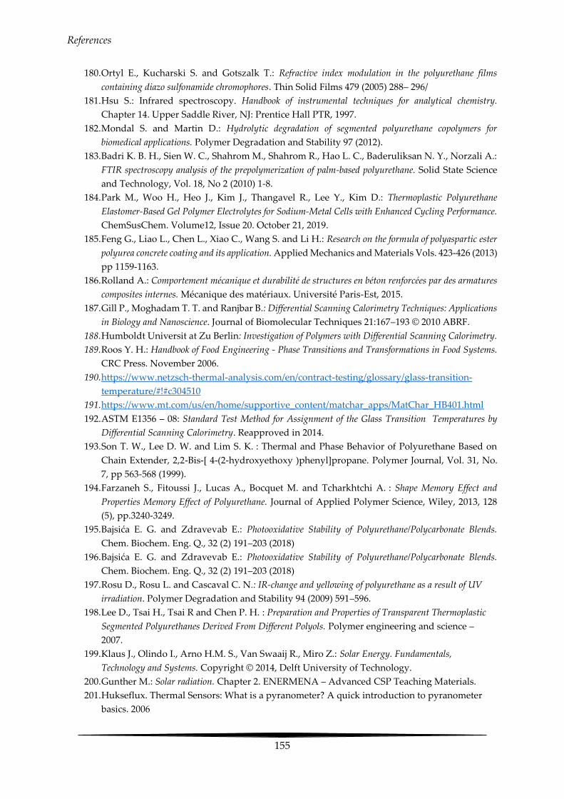
References
155
180. Ortyl E., Kucharski S. and Gotszalk T.: Refractive index modulation in the polyurethane films
containing diazo sulfonamide chromophores. Thin Solid Films 479 (2005) 288– 296/
181. Hsu S.: Infrared spectroscopy. Handbook of instrumental techniques for analytical chemistry.
Chapter 14. Upper Saddle River, NJ: Prentice Hall PTR, 1997.
182. Mondal S. and Martin D.: Hydrolytic degradation of segmented polyurethane copolymers for
biomedical applications. Polymer Degradation and Stability 97 (2012).
183. Badri K. B. H., Sien W. C., Shahrom M., Shahrom R., Hao L. C., Baderuliksan N. Y., Norzali A.:
FTIR spectroscopy analysis of the prepolymerization of palm-based polyurethane. Solid State Science
and Technology, Vol. 18, No 2 (2010) 1-8.
184. Park M., Woo H., Heo J., Kim J., Thangavel R., Lee Y., Kim D.: Thermoplastic Polyurethane
Elastomer‐Based Gel Polymer Electrolytes for Sodium‐Metal Cells with Enhanced Cycling Performance.
ChemSusChem. Volume12, Issue 20. October 21, 2019.
185. Feng G., Liao L., Chen L., Xiao C., Wang S. and Li H.: Research on the formula of polyaspartic ester
polyurea concrete coating and its application. Applied Mechanics and Materials Vols. 423-426 (2013)
pp 1159-1163.
186. Rolland A.: Comportement mécanique et durabilité de structures en béton renforcées par des armatures
composites internes. Mécanique des matériaux. Université Paris-Est, 2015.
187. Gill P., Moghadam T. T. and Ranjbar B.: Differential Scanning Calorimetry Techniques: Applications
in Biology and Nanoscience. Journal of Biomolecular Techniques 21:167–193 © 2010 ABRF.
188. Humboldt Universit at Zu Berlin: Investigation of Polymers with Differential Scanning Calorimetry.
189. Roos Y. H.: Handbook of Food Engineering - Phase Transitions and Transformations in Food Systems.
CRC Press. November 2006.
190. https://www.netzsch-thermal-analysis.com/en/contract-testing/glossary/glass-transition-
temperature/#!#c304510
191. https://www.mt.com/us/en/home/supportive_content/matchar_apps/MatChar_HB401.html
192. ASTM E1356 – 08: Standard Test Method for Assignment of the Glass Transition Temperatures by
Differential Scanning Calorimetry. Reapproved in 2014.
193. Son T. W., Lee D. W. and Lim S. K. : Thermal and Phase Behavior of Polyurethane Based on
Chain Extender, 2,2-Bis-[ 4-(2-hydroxyethoxy )phenyl]propane. Polymer Journal, Vol. 31, No.
7, pp 563-568 (1999).
194. Farzaneh S., Fitoussi J., Lucas A., Bocquet M. and Tcharkhtchi A. : Shape Memory Effect and
Properties Memory Effect of Polyurethane. Journal of Applied Polymer Science, Wiley, 2013, 128
(5), pp.3240-3249.
195. Bajsića E. G. and Zdravevab E.: Photooxidative Stability of Polyurethane/Polycarbonate Blends.
Chem. Biochem. Eng. Q., 32 (2) 191–203 (2018)
196. Bajsića E. G. and Zdravevab E.: Photooxidative Stability of Polyurethane/Polycarbonate Blends.
Chem. Biochem. Eng. Q., 32 (2) 191–203 (2018)
197. Rosu D., Rosu L. and Cascaval C. N.: IR-change and yellowing of polyurethane as a result of UV
irradiation. Polymer Degradation and Stability 94 (2009) 591–596.
198. Lee D., Tsai H., Tsai R and Chen P. H. : Preparation and Properties of Transparent Thermoplastic
Segmented Polyurethanes Derived From Different Polyols. Polymer engineering and science –
2007.
199. Klaus J., Olindo I., Arno H.M. S., Van Swaaij R., Miro Z.: Solar Energy. Fundamentals,
Technology and Systems. Copyright © 2014, Delft University of Technology.
200. Gunther M.: Solar radiation. Chapter 2. ENERMENA – Advanced CSP Teaching Materials.
201. Hukseflux. Thermal Sensors: What is a pyranometer? A quick introduction to pyranometer
basics. 2006

References
156
202. https://www.kippzonen.com/News/572/The-Working-Principle-of-a-Thermopile-
Pyranometer#.XrFxJHtpw2w
203. https://www.kippzonen.com/News/572/The-Working-Principle-of-a-Thermopile-
Pyranometer#.XrFxJHtpw2w
204. Tennis P. D., Leming M. L. and Akers D. J.: Pervious Concrete Pavement. EB302.02, Portland
Cement Association, Skokie, Illinois, and National Ready Mixed Concrete Association, Silver
Spring, Maryland, USA, 2004, 36 pages.
205. Qin Y., Yang H., Deng Z. and He J.: Water Permeability of Pervious Concrete Is Dependent on the
Applied Pressure and Testing Methods. Advances in Materials Science and Engineering. 2015.
206. https://civildigital.com/compressive-strength-concrete-concrete-cubes/
207. Jiji L.M.: Heat Convection. City University of New York – Springer. 2006.
208. EAPA (European Asphalt Pavement Association): Asphalt pavements on bridge decks. June 2013.
209. https://www.munroinstruments.com/product/bath-shower-pendulum/
210. Solaimanian M. and Kennedy T. W.: Evaluation of the cape seal process as a pavement
rehabilitation alternative. Report No FHWA/TX-99/1788-S. October 1998
211. Bateman D.: Design guide for road surface dressing. Road Note 39. March 2016.
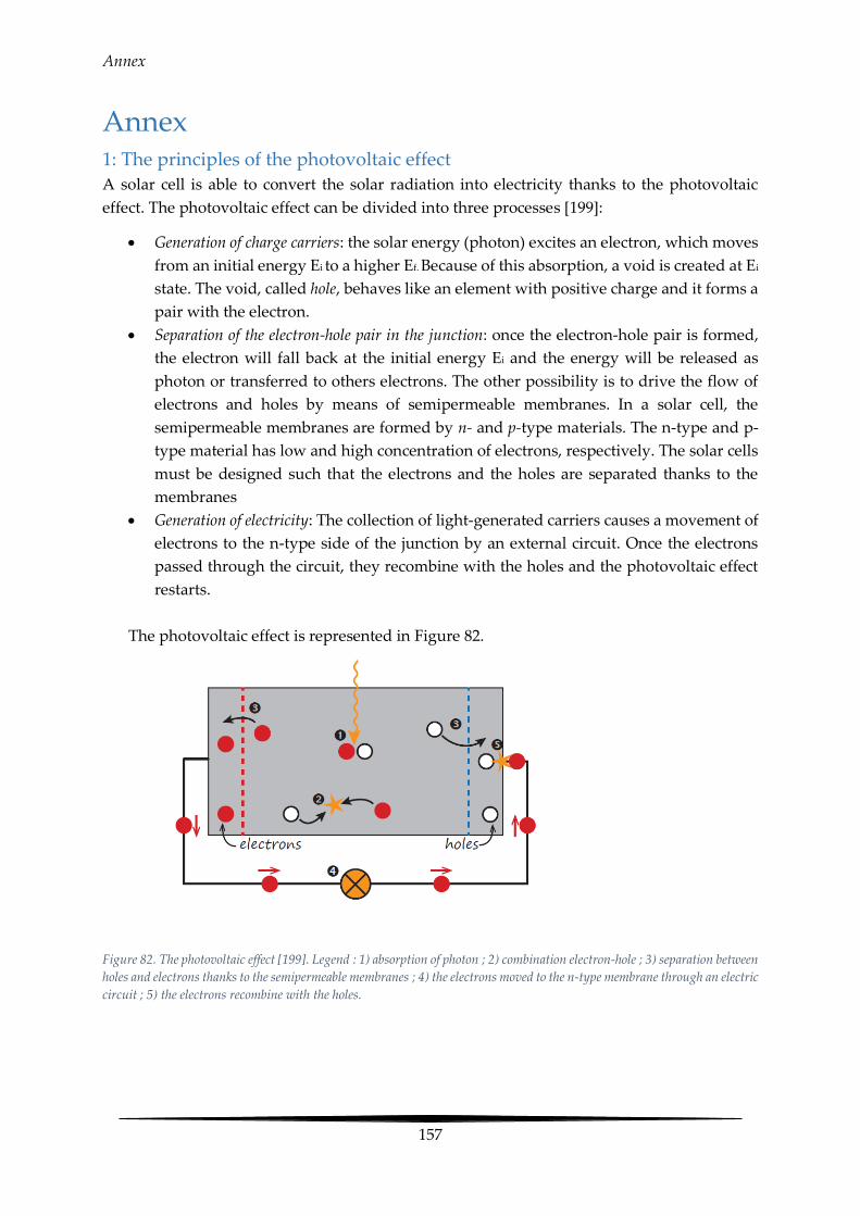
Annex
157
Annex 1: The principles of the photovoltaic effect
A solar cell is able to convert the solar radiation into electricity thanks to the photovoltaic
effect. The photovoltaic effect can be divided into three processes [199]:
Generation of charge carriers: the solar energy (photon) excites an electron, which moves
from an initial energy Ei to a higher Ef. Because of this absorption, a void is created at Ei
state. The void, called hole, behaves like an element with positive charge and it forms a
pair with the electron.
Separation of the electron-hole pair in the junction: once the electron-hole pair is formed,
the electron will fall back at the initial energy Ei and the energy will be released as
photon or transferred to others electrons. The other possibility is to drive the flow of
electrons and holes by means of semipermeable membranes. In a solar cell, the
semipermeable membranes are formed by n- and p-type materials. The n-type and p-
type material has low and high concentration of electrons, respectively. The solar cells
must be designed such that the electrons and the holes are separated thanks to the
membranes
Generation of electricity: The collection of light-generated carriers causes a movement of
electrons to the n-type side of the junction by an external circuit. Once the electrons
passed through the circuit, they recombine with the holes and the photovoltaic effect
restarts.
The photovoltaic effect is represented in Figure 82.
Figure 82. The photovoltaic effect [199]. Legend : 1) absorption of photon ; 2) combination electron-hole ; 3) separation between
holes and electrons thanks to the semipermeable membranes ; 4) the electrons moved to the n-type membrane through an electric
circuit ; 5) the electrons recombine with the holes.
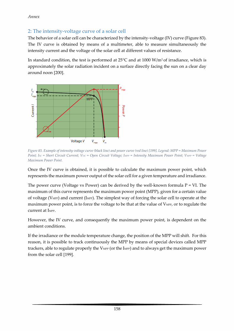
Annex
158
2: The intensity-voltage curve of a solar cell
The behavior of a solar cell can be characterized by the intensity-voltage (IV) curve (Figure 83).
The IV curve is obtained by means of a multimeter, able to measure simultaneously the
intensity current and the voltage of the solar cell at different values of resistance.
In standard condition, the test is performed at 25°C and at 1000 W/m2 of irradiance, which is
approximately the solar radiation incident on a surface directly facing the sun on a clear day
around noon [200].
Figure 83. Example of intensity-voltage curve (black line) and power curve (red line) [199]. Legend: MPP = Maximum Power
Point; ISC = Short Circuit Current; VOC = Open Circuit Voltage; IMPP = Intensity Maximum Power Point; VMPP = Voltage
Maximum Power Point.
Once the IV curve is obtained, it is possible to calculate the maximum power point, which
represents the maximum power output of the solar cell for a given temperature and irradiance.
The power curve (Voltage vs Power) can be derived by the well-known formula P = VI. The
maximum of this curve represents the maximum power point (MPP), given for a certain value
of voltage (VMPP) and current (IMPP). The simplest way of forcing the solar cell to operate at the
maximum power point, is to force the voltage to be that at the value of VMPP, or to regulate the
current at IMPP.
However, the IV curve, and consequently the maximum power point, is dependent on the
ambient conditions.
If the irradiance or the module temperature change, the position of the MPP will shift. For this
reason, it is possible to track continuously the MPP by means of special devices called MPP
trackers, able to regulate properly the VMPP (or the IMPP) and to always get the maximum power
from the solar cell [199].

Annex
159
3: Pyranometer
The pyranometer is a device able to measure the global irradiance, also called GHI (Global
Horizontal Irradiance), which is given by:
𝐸𝑔 = 𝐸 cos 𝜃 + 𝐸𝑑
Where:
- E is the maximum amount of direct sunlight;
- θ is the angle between the normal surface and the position of the Sun in the sky;
- Ed is the diffuse sunlight.
The GHI is expressed in W/m2 and it can ranges between 0 and 1400, depending on the
location, the position of the Sun, the meteorological conditions and presence of pollution [201].
The detection of the solar radiation is based on the Seebeck effect (see paragraph 1.1.3). The
device is composed by one or two domes, a black absorber and a thermopile21 (Figure 84).
Figure 84. Schematic representation of a pyranometer [202]. Legend: uout is the voltage output of the thermopile.
The dome is a glass for the protection of the black absorber, which allows the transmission of
the solar radiation in the range 300-3000 nm. The transmission is ideally 100%, but in practice
it is around 92%.
The solar radiation, which filters through the dome, is absorbed through the black surface and
converted into heat. In return, the absorbed heat causes a difference of temperature ΔT
between the black absorber and the thermopile. Because of the difference of temperature, the
thermocouples of the thermopile generate a voltage according to the Seebeck effect. If the
thermocouples are connected in series, the voltage of the thermopile is given by the sum of the
voltage of each thermocouple. On average, 1 W/m2 generates 10 μV [203].
In field, the pyranometer must be installed carefully, paying attention that the sensor is
perfectly horizontal aligned. Furthermore, the pyranometer requires a clear hemispherical
21 It is an electronic device able to convert the thermal energy into electrical energy

Annex
160
view (no obstacles for the sun radiation in surroundings). The presence of snow, frost or dust
on the dome surface could cause scattering of the solar radiation, leading erroneous
measurement. For this reason, some pyranometers are equipped with heaters and ventilation
systems.
Annex
161
4: Introduction to the prototype
The prototype, called RA2ROAD in honor of Ra (the Egyptian God of Sun), is a sandwiched
structure able to harvest energy exploiting the solar radiation. The system is able to generate
electricity thanks to some solar cells imbedded under a semi-transparent layer and, at the same
time, exploit the gradient temperature of the pavement, by means of a heat-transfer fluid
pumped in a porous layer.
The prototype is composed by the following layers (Figure 85):
- A semi-transparent top layer made of glass aggregates bonded together
through a transparent polyurethane;
- An electrical layer containing the solar cells;
- A porous concrete layer for the circulation of the heat-transfer fluid;
- A waterproof base layer.
Figure 85. Sketch of the prototype.
The semi-transparent layer
The semi-transparent layer is a composite material made of recycled glass aggregates bonded
together using a polyurethane glue which has to support the traffic load, guarantee the
vehicles friction, protect the solar cells, allow the passage of the sunlight and maximize the
heat transfer to the porous layer containing the heat-transfer fluid.
The manufacture of the semi-transparent layer has been carried out based on two different
approach named semi-transparent layer 1 (STL1) and semi-transparent layer 2 (STL2).
The STL1 consists of selecting two or more aggregate size classes (the procedure is the same
used to assess the particle size distribution of a granular material using standard sieves) and
mixing them together adding the polyurethane binder. Once the polymerization is completed,
the layer is placed directly on the solar cell.
More in detail, the manufacture procedure consists in: i) select two or more classes of
aggregates (i.e. 2/4mm and 4/6 mm); ii) weight each class according to the mix-design
specifications; iii) add a certain amount of binder; iv) mix the glass aggregates and the binder
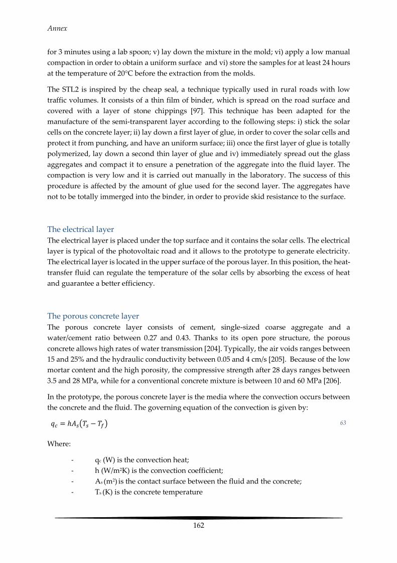
Annex
162
for 3 minutes using a lab spoon; v) lay down the mixture in the mold; vi) apply a low manual
compaction in order to obtain a uniform surface and vi) store the samples for at least 24 hours
at the temperature of 20°C before the extraction from the molds.
The STL2 is inspired by the cheap seal, a technique typically used in rural roads with low
traffic volumes. It consists of a thin film of binder, which is spread on the road surface and
covered with a layer of stone chippings [97]. This technique has been adapted for the
manufacture of the semi-transparent layer according to the following steps: i) stick the solar
cells on the concrete layer; ii) lay down a first layer of glue, in order to cover the solar cells and
protect it from punching, and have an uniform surface; iii) once the first layer of glue is totally
polymerized, lay down a second thin layer of glue and iv) immediately spread out the glass
aggregates and compact it to ensure a penetration of the aggregate into the fluid layer. The
compaction is very low and it is carried out manually in the laboratory. The success of this
procedure is affected by the amount of glue used for the second layer. The aggregates have
not to be totally immerged into the binder, in order to provide skid resistance to the surface.
The electrical layer
The electrical layer is placed under the top surface and it contains the solar cells. The electrical
layer is typical of the photovoltaic road and it allows to the prototype to generate electricity.
The electrical layer is located in the upper surface of the porous layer. In this position, the heat-
transfer fluid can regulate the temperature of the solar cells by absorbing the excess of heat
and guarantee a better efficiency.
The porous concrete layer
The porous concrete layer consists of cement, single-sized coarse aggregate and a
water/cement ratio between 0.27 and 0.43. Thanks to its open pore structure, the porous
concrete allows high rates of water transmission [204]. Typically, the air voids ranges between
15 and 25% and the hydraulic conductivity between 0.05 and 4 cm/s [205]. Because of the low
mortar content and the high porosity, the compressive strength after 28 days ranges between
3.5 and 28 MPa, while for a conventional concrete mixture is between 10 and 60 MPa [206].
In the prototype, the porous concrete layer is the media where the convection occurs between
the concrete and the fluid. The governing equation of the convection is given by:
𝑞𝑐 = ℎ𝐴𝑠(𝑇𝑠 − 𝑇𝑓) 63
Where:
- qc (W) is the convection heat;
- h (W/m2K) is the convection coefficient;
- As (m2) is the contact surface between the fluid and the concrete;
- Ts (K) is the concrete temperature
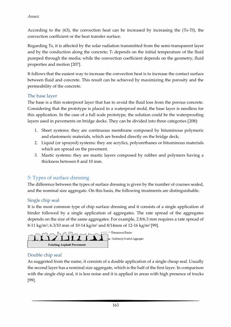
Annex
163
According to the (63), the convection heat can be increased by increasing the (Ts-Tf), the
convection coefficient or the heat transfer surface.
Regarding Ts, it is affected by the solar radiation transmitted from the semi-transparent layer
and by the conduction along the concrete; Tf depends on the initial temperature of the fluid
pumped through the media; while the convection coefficient depends on the geometry, fluid
properties and motion [207].
It follows that the easiest way to increase the convection heat is to increase the contact surface
between fluid and concrete. This result can be achieved by maximizing the porosity and the
permeability of the concrete.
The base layer
The base is a thin waterproof layer that has to avoid the fluid loss from the porous concrete.
Considering that the prototype is placed in a waterproof mold, the base layer is needless for
this application. In the case of a full scale prototype, the solution could be the waterproofing
layers used in pavements on bridge decks. They can be divided into three categories [208]:
1. Sheet systems: they are continuous membrane composed by bituminous polymeric
and elastomeric materials, which are bonded directly on the bridge deck;
2. Liquid (or sprayed) systems: they are acrylics, polyurethanes or bituminous materials
which are spread on the pavement.
3. Mastic systems: they are mastic layers composed by rubber and polymers having a
thickness between 8 and 10 mm.
5: Types of surface dressing
The difference between the types of surface dressing is given by the number of courses sealed,
and the nominal size aggregate. On this basis, the following treatments are distinguishable.
Single chip seal
It is the most common type of chip surface dressing and it consists of a single application of
binder followed by a single application of aggregates. The rate spread of the aggregates
depends on the size of the same aggregates. For example, 2.8/6.3 mm requires a rate spread of
8-11 kg/m2; 6.3/10 mm of 10-14 kg/m2 and 8/14mm of 12-16 kg/m2 [99].
Double chip seal
As suggested from the name, it consists of a double application of a single cheap seal. Usually
the second layer has a nominal size aggregate, which is the half of the first layer. In comparison
with the single chip seal, it is less noise and it is applied in areas with high presence of trucks
[99].
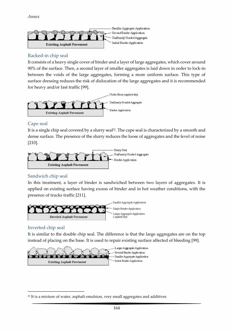
Annex
164
Racked-in chip seal
It consists of a heavy single cover of binder and a layer of large aggregates, which cover around
90% of the surface. Then, a second layer of smaller aggregates is laid down in order to lock-in
between the voids of the large aggregates, forming a more uniform surface. This type of
surface dressing reduces the risk of dislocation of the large aggregates and it is recommended
for heavy and/or fast traffic [99].
Cape seal
It is a single chip seal covered by a slurry seal22. The cape seal is characterized by a smooth and
dense surface. The presence of the slurry reduces the loose of aggregates and the level of noise
[210].
Sandwich chip seal
In this treatment, a layer of binder is sandwiched between two layers of aggregates. It is
applied on existing surface having excess of binder and in hot weather conditions, with the
presence of trucks traffic [211].
Inverted chip seal
It is similar to the double chip seal. The difference is that the large aggregates are on the top
instead of placing on the base. It is used to repair existing surface affected of bleeding [99].
22 It is a mixture of water, asphalt emulsion, very small aggregates and additives

Annex
165
5: The British pendulum test
The British Pendulum test [155] is a low-cost device for the measurement of the pavement
skid-resistance. It is composed by a natural rubber slider mounted at the end of the pendulum.
The distance between the center of swing and the test surface is 508mm, while the contact path
between slider and sample is 125 ± 1.6 mm or 76-78 mm for flat test surfaces and polishing-
wheel specimens, respectively (Figure 86).
Figure 86. Example of British pendulum test [209].
The test procedure consists in: 1) apply water on the sample surface; 2) let fall the pendulum
from its initial position (parallel to the surface); 3) catch the pendulum during the return swing,
before the slider hits the sample; 4) read the British Pendulum Number (BPN) value indicated
on the graduated scale; 5) repeat the test four times and calculate the average BPN.
Finally, the BPN value can be compared with the specifications of Table 34.

Annex
166
Category Type of Site BPN on Wet
Surfaces
Standard of Skidding
Resistance Represented
A
Most difficult sites such as; i)-
Roundabouts ii)- Bends with radius
less than 500 ft on derestricted roads.
iii)- Gradients, 1 in 20 or steeper, of
length greater than 100 yd. iv)-
Approach to traffic lights on
derestricted roads.
Above 65
Good: fulfilling the
requirements even of fast
traffic, and making it most
unlikely that the road will be
the scene of repeated
accidents.
B
General requirements, i.e. roads and
conditions not covered by categories
A & C.
Above 55
Generally Satisfactory:
meeting all but the most
difficult conditions
encountered on the roads.
C
Easy sites, e.g. straight roads, with
easy gradients and curves, without
junctions, and free from any features,
such as mixed traffic, especially liable
to create conditions of emergency.
Above 45 Satisfactory: only in
favorable circumstances
D All Sites Below 45 Potentially Slippery
Table 34. Skid resistance specifications [156].

Annex
167
6: Plots of E’, E’’ and tan(δ) according to generalized Maxwell for the glue B, C
and D

Annex
168
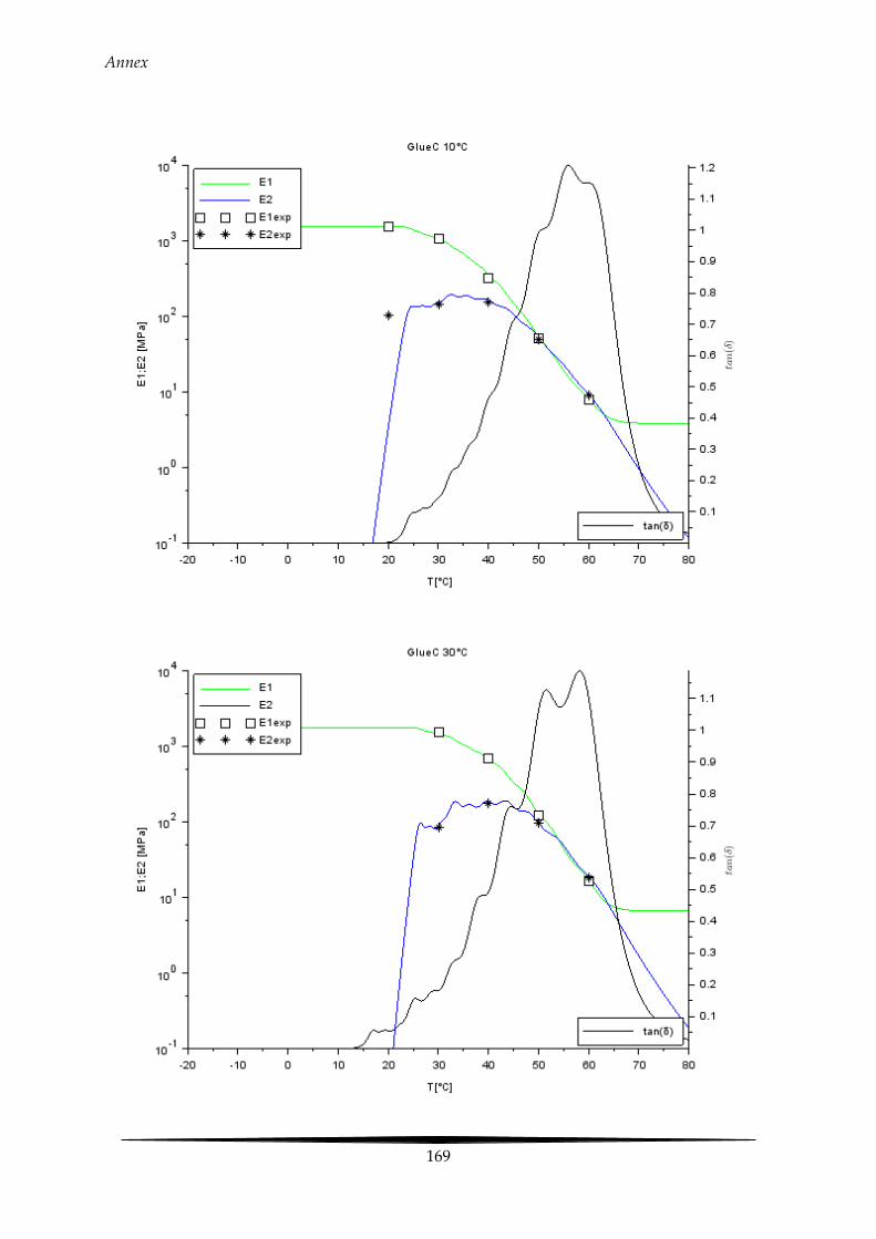
Annex
169

Annex
170

Annex
171

Annex
172
7: FTIR of glue B

Annex
173
8: FTIR of glue D
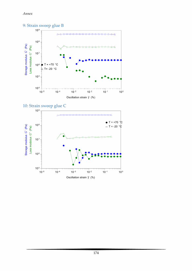
Annex
174
9: Strain sweep glue B
10: Strain sweep glue C
Glue C(1) unaged strain sweep

Annex
175
11: Strain sweep glue D
Glue D(1) unaged strain sweep
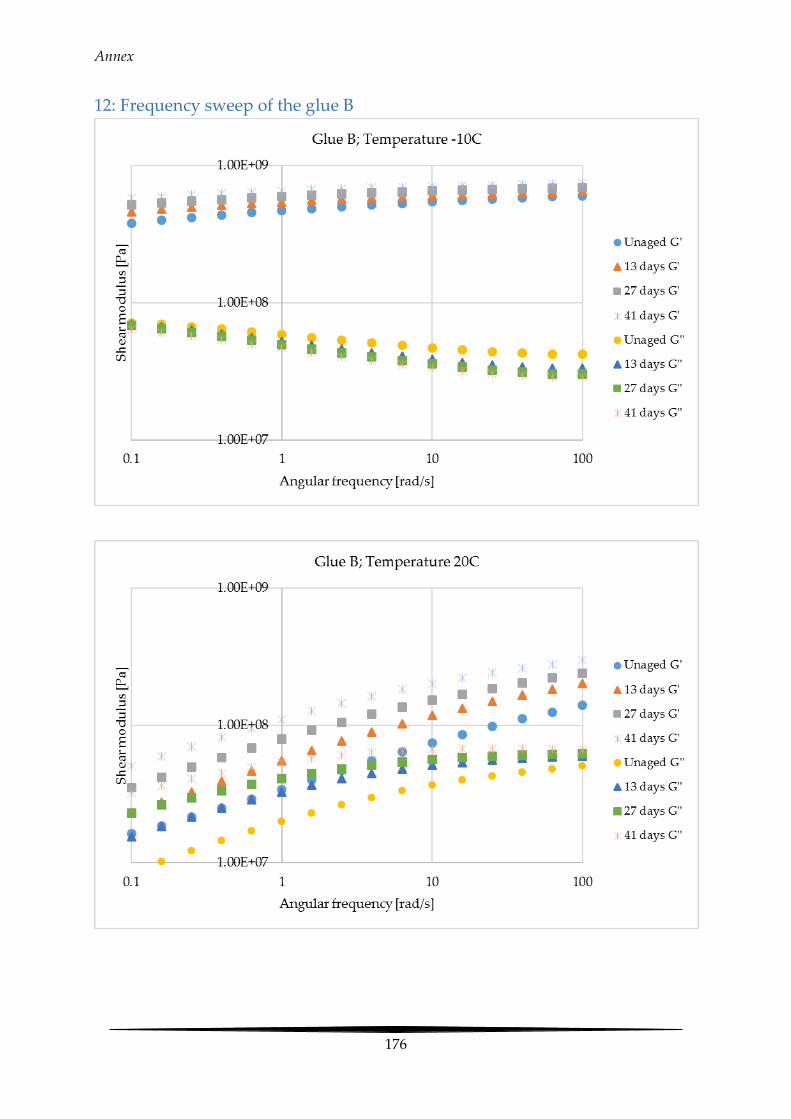
Annex
176
12: Frequency sweep of the glue B
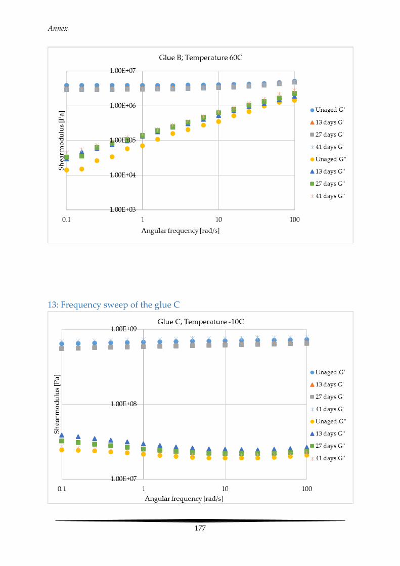
Annex
177
13: Frequency sweep of the glue C

Annex
178

Annex
179
14: Frequency sweep of the glue D
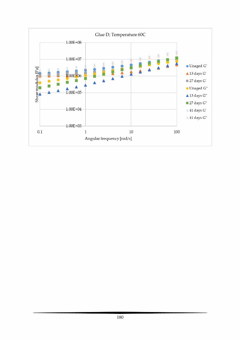
180


Titre : Mix-design d'une nouvelle couche semi-transparente pour les routes solaires
Mots clés : Récupération d'énergie, route solaire, couche semi-transparente, polyuréthane
Résumé : Le réseau routier du futur ne sera pas simplement un système de transport pour les utilisateurs et les biens, mais aussi une technologie pour la récupération d'énergie, profitant des surfaces existantes. Cette thèse traite de la formulation d'une couche semi-transparente pour les routes solaires. La nouvelle surface est un matériau composite constitué de granulats de verre lié entre eux par une colle polyuréthane. A l’heure actuelle il n'existe aucune préconisation pour l’emploi de liant polyuréthane sur les couches de surface. Pour cette raison, 4 colles polyuréthanes sont caractérisé en termes de cinétique de polymérisation et de propriétés viscoélastiques. La recherche se focalise ensuite sur la formulation de la couche semi-transparente en se basant sur trois méthodes/techniques: la compacité de l’empilement granulaire, le plan d’expérience et la technique de l’enduit superficiel.
L'objectif est l'optimisation à la fois optique et mécanique du matériau, dans la perspective d'une application à l’echelle 1. La dernière étape est la compréhennsion du vieillissement de la colle par le rayonnement solaire au moyen des techniques FTIR, DSC et rhéomètre rotationnel. La formulation de la couche semi-transparente est une étape importante vers la réalisation de la "route hybride", un système dédié à la récupération d'énergie né de l'union d'une route photovoltaïque avec un milieu poreux capable d'extraire de l'énergie temrique au moyen d'un fluide caloporteur.
Title : Mix-design of a novel semi-transparent layer for solar roads
Keywords : Energy harvesting, solar road, semi-transparent layer, polyurethane
Abstract : The road network of the future will be not only a transportation system for people and goods, but also a technology able to harvest energy from the Sun exploiting existing surfaces. This manuscript deals with the mix-design of a semi-transparent layer for solar roads. The novel surface is a composite material given by recycled glass aggregates bonded together using the polyurethane. At present, there are no specifications or guidelines for the use of the polyurethane in solar roads. In the light of this, the polyurethane is characterized in terms of curing kinetic and viscoelastic behavior performing the DSR and the DMA. The research also focuses on the mix-design of
the semi-transparent layer based on three methods/techniques: the packing density, the fraction factorial design and the surface dressing. The objective is to optimize the optical and mechanical performance of the mixture, in the prospective of a full scale application. Finally, the aging of the polyurethane because of the UV exposition is investigated by means of the FTIR, the DSC and the rotational rheometer test. The mix-design of the semi-transparent layer is an important step towards the manufacture of the “hybrid road”, a road energy harvesting system obtained by the union between a concrete porous medium used as solar collector with a photovoltaic road.