model-based development and simulation for robotic systems ...cdn.intechopen.com/pdfs/42783.pdf ·...
TRANSCRIPT
International Journal of Advanced Robotic Systems Model-Based Development and Simulation for Robotic Systems with SysML, Simulink and Simscape Profiles Regular Paper
Mohd Azizi Abdul Rahman1,2,* and Makoto Mizukawa3
1 Graduate School of Engineering, Shibaura Institute of Technology, Tokyo, Japan 2 University of Technology Malaysia, Kuala Lumpur International Campus, Malaysia 3 Department of Electrical Engineering, Shibaura Institute of Technology, Tokyo, Japan * Corresponding author E-mail: [email protected] Received 30 May 2012; Accepted 17 Dec 2012 DOI: 10.5772/55533 © 2013 Rahman and Mizukawa; licensee InTech. This is an open access article distributed under the terms of the Creative Commons Attribution License (http://creativecommons.org/licenses/by/3.0), which permits unrestricted use, distribution, and reproduction in any medium, provided the original work is properly cited.
Abstract In system‐level design, it is difficult to achieve a system verification which fulfils the requirements of various stakeholders using only descriptive system models. Descriptive system models using SysML alone are insufficient for system behaviour verifications and engineers always use different simulation tools (e.g., the Mathworks Simulink or Modelica Dymola) to analyze systems behaviour. It is a good idea to combine descriptive and simulation models. This paper presents the development of a collaborative design framework which brings SysML, Simulink, and Simscape profiles within the domain of robotics. A conceptual design method is proposed to support execution models for simulation. In brief, the descriptive SysML system‐level model is interpreted into the system‐level simulation models (e.g., Simulink and Simscape). We then use a plugin‐based model integration technique to keep both models in sync for automatic simulation. A simulation study is performed to evaluate the system. To illustrate the design of this system, we present a simulated closed‐loop system.
Keywords Model Based Development, Robotic System‐Level Design, OMG SysML™, Simulink®, IBM® Rational® Rhapsody®, Simscape™
1. Introduction
Robots can be regarded as complex systems due to the collection of interrelated components and systems engineering principles are required in their design [1]. Moreover, the integration of components from the very beginning of the design process can result in extremely complicated design decisions. A combined operation of multiple domains such as mechanical, electrical, control and software is needed to manage all the system functionalities. To help engineers deal with the increasing complexity in systems design, a model‐based approach can be adopted. Model‐based system engineering (MBSE), a recent development, has become an accepted approach for designing complex systems [2]. MBSE has been introduced as a mainstream method which involves a fundamental shift from traditional document‐centric
1Mohd Azizi Abdul Rahman and Makoto Mizukawa: Model-Based Development and Simulation for Robotic Systems with SysML, Simulink and Simscape Profiles
www.intechopen.com
ARTICLE
www.intechopen.com Int J Adv Robotic Sy, 2013, Vol. 10, 112:2013
approaches to computerized model‐based approaches [3]. In addition to MBSE, a graphical‐based language for enabling systems engineering activities, the OMG SysML™ [4] has been standardized based on UML [5] in support of the MBSE framework. Using MBSE in systems design, engineers can solve systems engineering problems by expressing multiple views that can transform stakeholders’ requirements into detailed specifications with the aid of models [6]. In this paper, we propose a comprehensive system‐level design workspace for robotics in conjunction with the simulation of continuous system dynamics. The primary modelling languages are introduced, such as SysML™ for systems engineering activities, Simscape™ [7], the declarative language for physical systems modelling and also Simulink® [8], Matlab’s extension product that allows the modelling and simulation of continuous processes using block diagrams. For this study, the UML modelling tool, the IBM® Rational® Rhapsody® software [9] is used to design system‐level models based on the SysML profile. The simulation environment is set to Simulink. In brief, the system model of the robot is first described using SysML to represent the continuous‐time dynamics behaviour of the system. A new set of stereotypes is created in order to provide distinctive model semantics in support of Simulink‐ and Simscape‐compatible models. A subsystem that contains components, for example, actuators, sensors, and the base platform is then modelled based on a physical system modelling approach using a Simscape language. Lastly, all the models are integrated and synchronized with the system‐level simulation model and be executed in the Simulink window automatically. The remainder of the paper is organized as follows. Some related works are reviewed in section 2 which consider continuous behaviour modelling and systems model integration of different languages. Section 3 describes the proposed method with the aid of a case study. The modelling of the continuous system dynamics and the whole model composition are presented in greater detail in section 4. Section 5 briefly discusses model integration and how the models are kept in sync, including implementation and simulation results. Last but not least, section 6 gives a summary of the proposed method and describes some possible future works.
2. Related Research
For this section, related works on continuous behaviour modelling, model semantics extension and systems model integration of different languages are reviewed. According to Bruninyckx [10], robotics is a field of integration rather than a fundamental science, so it contributes to complex systems integration. In that sense, robotic systems that typically consist of multi‐domain
aspects need a new conceptual framework for multi‐system integration in the later stages of development. Recent contributions to the development of robot systems that use the potential of SysML language are presented in [11] for the design of a space robotics system, in [12] for the software development process of a mobile robot and in [13] for a SysML‐based robot systems design for manipulation tasks. We seek to investigate the potential uses of SysML in the field of robotics, control and systems engineering. SysML was developed as a general‐purpose modelling language that is only capable of descriptive semantics. Executable semantics are required for the design of the simulation and its analysis. Associating executable semantics with SysML descriptive semantics can be realized by developing an extension to the UML model element [14]. Johnson et al. [15‐16] proposed a formal technique for modelling continuous system dynamics in SysML through language mapping between SysML constructs and the declarative Modelica [17] language. The mapping method uses the extension of SysML model elements through the stereotypes mechanism rather than formulating totally new language constructs. As a result, compatible SysML constructs are established for selected Modelica elements in representing the continuous dynamics modelling constructs, as well as their simulation model in SysML. Venderperren and Dehaene [18], and Kawahara et al. [19] discussed a co‐simulation approach using UML/SysML and Matlab/Simulink, in which a software‐based coupling tool is used to combine the UML/SysML model and the simulation model in Simulink. For mechatronic system behaviour, Turki and Soriano [20] proposed a method for representing continuous dynamics behaviour using a bond graph based on the extension of SysML activity diagrams. Furthermore, Cao et al. [14] recently introduced a mixed‐behaviour system‐level design using SysML, and Stateflow and Simscape for system‐level simulation. In addition, a model semantic extension is carried out based on the stereotypes mechanism [21]. Based on the above information, we believe that the system‐level design and simulation technologies which use the potential of SysML, Simulink and Simscape could offer promising solutions for robotics and its applications.
3. Method
This section describes the methodology used in the system‐level modelling, simulation and control of a wheeled mobile robot. From control engineering perspectives, the design of control dynamic systems works well using a model‐based design (MBD) approach with a widely‐used design software and simulation, (e.g., Matlab/Simulink). Simulink uses block diagrams, whose
2 Int J Adv Robotic Sy, 2013, Vol. 10, 112:2013 www.intechopen.com

syntax is familiar to control engineers [19]. However, they often lack understanding of how to provide proper specifications for the system they design which leads to unmanageable and inconsistent system specifications. In contrast, system engineers are capable of preparing those specifications in a highly manageable way from the conceptual abstraction design to the detailed design. Therefore, our proposed framework will let the system and domain experts (e.g., systems design engineers, software developers and control engineers) collaborate from the first until the last development stages within a unified workspace.
3.1 A Brief Overview of the method
A significant trend in contemporary systems engineering practice is model‐based designs, which make use of explicit models to define activities in the life cycle of the design and development of products [22]. To create system‐level design and simulation models, we need to define the system structure and its behaviour (continuous‐time). SysML provides several constructs for defining the system’s structure and behaviour. For this study, the Simulink‐ and Simscape‐related models are semantically defined in SysML to obtain a newly compatible structure and simulatable models. The continuous system behaviour will then be assigned to a SysML block by referencing the Simulink and Simscape models from the block. A plugin‐based model integration is performed to sync the SysML design model with the Simulink‐ and Simscape‐compatible model, and thus generate the simulatable model automatically. Prior to that, simulation properties need to be configured, (e.g., the solver type, solver name, and start/stop time). The proposed method is illustrated by using a wheeled mobile robot system.
3.2 An example system
The physical system and its behaviour are usually formed in terms of differential equations. In this paper, a simplified closed‐loop system, as shown in Fig.1, is used as a case study. The system simply consists of two main subsystems and several components: the robot base (i.e., including its body dynamics and kinematics components) with embedded actuators and sensors (e.g., both translational and rotational sensors), a control system and the desired input in the form of a position in the X‐Y coordinate system and the desired orientation (e.g., xd, yd, θd). The robot base is a symmetrical round‐shaped mobile platform with two actuated wheels and one passive wheel (not shown in the figure) that is placed in front of the platform for stability. The physical properties of the robot platform are the mass (m), the radius of robot’s base from the centre of the robot platform (rc), the robot’s wheel radius (rw), the robot’s
width (wd), and the robot’s base moment of inertia (Ib) about the vertical axis. The following shows mathematical representations of the system:
s (1)
(2)
r l wm v t t / r
(3)
b c d r l2 r / w t t
(4)
Note that the representation reflects Newton’s second‐order law of motion and the energy‐based Euler‐Lagrange formulation where s, v, θ, and ω represent the robot’s displacement, forward velocity, orientation and angular velocity respectively. tr and tl denote the applied torques to the right and left wheel of the robot, respectively.
Figure 1. Closed‐loop wheeled mobile robot system
Furthermore, the robot’s motion on a horizontal plane with the kinematics constraint of the system is represented by the following equations [23]:
x s cos( ) (5)
y s sin( ) (6)
where, (x, y) denotes the robot’s position in the X‐Y reference frame. The measured variables (x, y, θ) will be compared to the desired input and fed to the controller as the error term (e.g., e = [ex, ey, eθ]T = [xd‐x, yd‐y, θd‐θ]T). The control algorithm is simplified by the following equations:
l 1 2 3deu K e K e dt Kdt
(7)
r 1 2 3
deu K e K e dt Kdt
(8)
where, ul and ur denote the controller left‐ and right‐output, respectively. K1, K2, and K3 represent the tunable coefficients for controller gains. The objective of the controller is to provide appropriate torques (tl, tr) to be applied to the robot for motion. Therefore, the robot will be controlled based on the torques applied to the left‐ and right‐side of the wheels.
θ
s
x
y
tr
tlController
txd, yd, θd
x, y, θ
ex, ey, eθ
3Mohd Azizi Abdul Rahman and Makoto Mizukawa: Model-Based Development and Simulation for Robotic Systems with SysML, Simulink and Simscape Profiles
www.intechopen.com

4. System Definition View in SysML
The SysML’s block is the most utilized model element for describing both logical and physical objects of complex systems [4]. It is the basic construct of the SysML model. For conceptual system‐level definition, the closed‐loop system as shown in Fig.1 is firstly defined in a hierarchical way using the SysML block definition diagram (BDD). This is shown in Fig.2 where the ‘ClosedLoopSystem’ block is viewed as a basis for the simulation of the main structure of the system. As we can see, the ‘ClosedLoopSystem’ block is composed of one or more ‘SimulinkSubsystem’, and one or more ‘SimscapeSubsystem’. Note that the subsystem block is directly composed to the system block by using the black‐diamond‐arrow relation. Down to the component level, the ‘SimulinkSubsystem’ is made up of zero or more ‘Input’ and one or more ‘Controller’ blocks. The ‘SimscapeSubsystem’ is made up of one ‘Body’, one or more ‘Actuator’, one or more ‘Sensor’ and zero or more ‘Kinematics’ blocks.
Figure 2. Conceptual system definition view
The SysML descriptive model needs to be defined as executable models, which can then be translated into the analysis model for use in the simulation tool. Toward this end, SysML model definition and its semantic extension should be done in order to support the behavioural design models and the integration of a simulation model. For extension of the SysML model, we use the stereotype mechanism [21, 24]. The stereotype mechanism is widely adopted to semantically extend the SysML model and is a powerful way to define a new SysML model element by tailoring the UML meta‐model [24]. Stereotypes are visually spotted by looking at the keyword within a set of double chevrons (e.g., <<stereotype>>). A model semantic extension can be carried out using two techniques [14]: either the “heavy‐weight” or the “light‐weight” approach. By comparison, the first approach develops totally new constructs for the SysML profile, while the second technique simply creates a new profile of stereotypes based on the UML’s meta‐class for extending the SysML model element [20]. However, the first method requires a distinctive tool to support the new construct [21]. For this reason, we apply the second
method because it is more easily implemented in our current SysML tool. Based on the above analysis, we choose to model the system in SysML using a component‐based approach, in which the closed‐loop system is first decomposed into several components with their associated functions. The extension of the model is then implemented on SysML blocks to design the Simulink‐ and Simscape‐compatible models. Thus, a set of new stereotypes is defined to associate the SysML constructs with the new model element capability. As a result, the design and analysis models of the system are prepared and we apply the physical system modelling approach to construct an energy‐flow physical system network. The physical modelling network is considered as a group of interrelated subsystems and/or components that are linked to one another through their energy ports [25].
4.1 SysML‐Simulink Model Compatibility
In this subsection, the definition of the SysML‐Simulink compatibility model is illustrated with regards to the input and controller components.
4.1.1 SimulinkBlock (SB) Stereotype
This section briefly describes the concept of the SysML model extension in defining the SysML‐Simulink compatible model. As mentioned earlier in section 4, it is based on the stereotype mechanism that tailors the SysML meta‐model to create a new model element. The concept of meta‐modelling is briefly described in [24]. The element that needs to be stereotyped is a standard SysML block taken from the meta‐model. Fig.3 shows the definition of a new stereotype extended to support Simulink models. It introduces two blocks associated with a specialization relation (the solid arrow), known as the extension relationship, (e.g., <<extend>>). It should be noted that the standard SysML block now becomes a special block that happens to be a Simulink reference model representation. Specifically, the semantics of the SB, when it is applied to a SysML block, will be referred to a Simulink model encapsulation. Therefore, the SB represents a wrap model in Simulink. Apart from semantic extension, the SB stereotype declares tagged values with which to indicate auxiliary properties of the Simulink model. For example, the ‘URI’ property that provides a link to the Simulink model files. Optionally, tagged values can be used to add information to the model base, specific to the domain or platform [26]. Fig.4 shows a BDD that illustrates the “Input” and “Controller” blocks. As we can see, both components apply the SB stereotype. Equations (7)‐(8) are properly described in the “Controller” block (shown by the use of the stereotype, <<Algorithm>>) along with its gain parameters, error variables (shown by the stereotype,
ClosedLoopSystem«block»
::SimulationContext::
SimulinkSubsystem«block»
1..*subsys1 1..*subsys1
SimscapeSubsystem«block»
1..*subsys2 1..*subsys2
Input«block»
*comp1 *comp1
Controller«block»
1..*comp2 1..*comp2 1comp3
Body«block»
1comp3 *comp4
Kinematics«block»
*comp4 1..*comp6
Actuator«block»
1..*comp61..*comp5
Sensor«block»
1..*comp5
4 Int J Adv Robotic Sy, 2013, Vol. 10, 112:2013 www.intechopen.com

<<Error>>) and data ports, while the system input information is appropriately defined in the “Input” block which consists of input variable values and a single output data port.
Figure 3. Definition of SB
Figure 4. Simulink‐related model definition in SysML
The constraint compartment can be used to describe system equations either in the continuous or discrete behaviour. Note that not only a model element is extended but also all the information contained in the block. For example, the stereotype, <<Gain>> emulates the tunable parameters of the controller while the ports extend the standard SysML flow port applicable to the in‐port and out‐port of the Simulink‐compatible model. The data type is assigned as the real value, for example, “real_T”.
4.2 SysML‐Simscape Model Compatibilty
4.2.1 Simscape Language Overview
In this section, we give an overview of the Simscape language. We use the Simscape language to customize our system components rather than using an existing Simscape foundation library. Basically, there are two model types, the domain and component files, available in the Simscape language [27]. The former is used to define the physical system domain (e.g., electrical, rotational, translational, hydraulic, etc) and corresponds to the port types, in which the component exchanges the energy‐type
element. The latter model type is used to define the physical component that users intend to model in corresponding to the Simscape block (e.g., resistors, capacitors, inductors, and etc). It is essential to understand the basic file format for the domain and component models. Examples of both domain and component files are shown below: 1. The domain model for RotationaL.ssc domain RotationaL %Declaration section variables w = {1,‘rad/s’};%Across variable end variables t = {1,‘N*m’};%Through variable end end 2. The component model for sensor.ssc component sensor %Declaration section nodes R = CLib.RotationaL;%Energy port T = CLib.TranslationaL;%Energy port end outputs S = {0,‘m’};%Signal port A = {0,‘rad’};%Signal port end parameters Init_theta = {0,‘rad’};%Initialize Init_s = {0,‘m’};%Initialize end variables w = {0,‘rad/s’};%Across var v = {0,‘m/s’};%Across var theta = {0,‘rad’};%Across var s = {0,‘m’};%Across var end function setup %Implementation section across(w, R.w,[]); across(v, T.v,[]); s = init_s; theta = init_theta; end equations s.der == T.v; S == s; %Displacement measure theta.der == R.w; A == theta; %Angle measure end end A Simscape file separates the model description into the following properties: the declaration and implementation sections. The declaration section, which imitates the
<<extend>>
SysML«block»
SimulinkBlock«S tereoty pe»
Input«block,S imulinkBlock»
Values
«Input» xd:real_T=m«Input» yd:real_T=m«Input» thetad:real_T=rad
Ports
out:real_T
Controller«block,S imulinkBlock»
Values
«Error» ex:real_T«Error» ey:real_T«Error» etheta:real_T«Gain» K1:real_T«Gain» K2:real_T«Gain» K3:real_T
Ports
in:real_Ttheta:real_Tul:real_Tur:real_Tx:real_Ty:real_T
Constraints
«Algorithm» {ul = [K1,K2,K3]*[ex;ey;etheta]};«Algorithm» {ur = [K1,K2,K3]*[ex;ey;etheta]};
5Mohd Azizi Abdul Rahman and Makoto Mizukawa: Model-Based Development and Simulation for Robotic Systems with SysML, Simulink and Simscape Profiles
www.intechopen.com
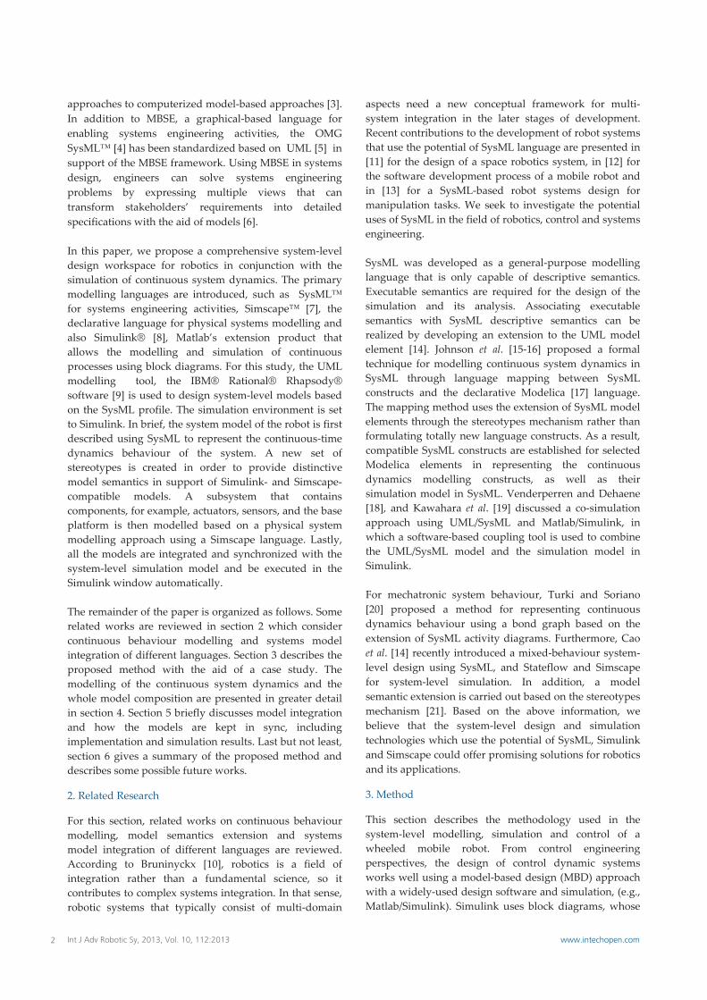
Matlab class declaration method, includes member classes such as nodes, inputs and/or outputs, parameters, and variables for both domain and component files. Note that for the domain file, only variables and sometimes parameters (optional) are declared so that their function is to establish a domain rather than a detailed component. In contrast, the implementation section includes only the setup function and equations for the component file. In the setup function, the component is prepared for simulation and it is executed once for each component during the model compilation process whereas the equations section declares the component equations that are executed throughout the simulation. Therefore, the implementation section is utilized to establish an equation‐based internal behaviour of the system. More detail on the Simscape model structure, can be found in references [7] and [27]. Although Simscape is conceptually more specific to the physical system theory, it can fit to the general concept used in Matlab/Simulink. Thus, it allows for Simscape models to be combined with other models in the same Simulink environment.
4.2.2 SysML Model Extension for Simscape
The SysML block is again semantically extended to represent the domain and component model in Simscape. Since the domain model has no internal behaviour, the stereotype <<Domain>> is newly defined relative to its semantics [14]. Fig.5 illustrates the newly defined ‘TranslationaL’ and ‘RotationaL’ domains, and the ‘Body’ component block. The physical component is clearly defined by the stereotype, <<Comp>>. A SysML block has value properties, which are referred to as value types. These are utilized to define system variables, parameters, constants and other properties of component models in Simscape. The stereotypes such as <<Across>> and <<Through>> are created for physical system domain variables [25], and to differentiate variables among other common properties. For example, the stereotype named <<Parameters>> defines the mass property of the physical component with the value type, kilogram. The nodes, inputs and outputs of the component are modelled by utilizing the SysML’s flow port. In SysML, the ‘eneryport’ is defined to replicate the Simscape bi‐directional conserving port which allows only energy‐based elements to pass through it. It is based on the non‐atomic flow port where multiple items can exchange energy through the ports. As mentioned in 4.2.1, the setup and equations properties are for the implementation part of the Simscape model. They are represented as constraints in SysML and describe the syntax with which the attributes of objects should comply. Thus, the stereotype <<Init>> has been defined to distinguish
between the function setup process and the variable initialization process. For example, the constraint “R.w == theta.der”, represents the time derivative of the orientation angle, which gives a solution to the angular velocity variable, on the other hand, the constraint “theta == init_theta”, declares the initial condition setup for the orientation angle. In Fig.6, the kinematics, actuator and sensor blocks are stereotyped with <<Comp>> similar to the ‘Body’ block. The kinematics for the system is described based on equations (5) and (6). The actuated wheels receive control outputs through the signal ports (i.e., tr and tl), and apply the torque to both wheels of the robot via the energy port, T. The sensor can be used to detect the state variables changes, and send them as data via the signal port. For the Simscape subsystem block, the stereotype <<SimscapeBlock>> (see Fig.8) is introduced as an extended SysML block that applies the same concept and property for the SB. Therefore, all Simscape‐related blocks can also apply the SB stereotype.
Figure 5. Definition of Simscape domain models and the body component
Rotat ionaL«Domain»
Attributes
«Through» t:real_T=N*m«Across» w:real_T=rad/s
T ranslationaL«Domain»
Attributes
«Through» f :real_T=N«Across» v :real_T=m/s
Body«block,Comp»
Values
«Nodes» RotationaL:real_T=R«Nodes» TranlationaL:real_T=T«Parameters» m:real_T=k g«Parameters» rc:real_T=m«Parameters» wd:real_T=m«Parameters» Ib:real_T=k gms 2̂«Init» init_s:real_T=m«Init» init_theta:real_T=rad«Across» w:real_T=rad/s«Across» v :real_T=m/s«Across» s :real_T=m«Across» theta:real_T=rad«Through» f :real_T=N«Through» t:real_T=Nm
Ports
energyport_R:in_outenergyport_T:in_out
Constraints
«Setup» through(f ,T.f ,[ ]);«Setup» through(t,R.t,[ ]);«Setup» ac ross(v ,T.v ,[ ]);«Setup» ac ross(w,R.w,[ ]);«Setup» s = init_s ;«Setup» theta = init_theta;«Equations» T.v = = s.der;«Equations» R.w = = theta.der;«Equations» m*T.v .der = = f ;«Equations» 2*Ib*rc *R.w.der/wd = = t;
6 Int J Adv Robotic Sy, 2013, Vol. 10, 112:2013 www.intechopen.com

The syntax used in the setup function and the equation section conform to the Simscape language [27]. Note that writing the equations with the operator ‘= =’, means that they do not constitute the assignment operator but rather a symmetrical mathematical relationship exists between both left‐ and right‐hand operands, and they are evaluated continuously throughout the simulation process. Apart from that, the value unit at both the left‐ and right‐hand sides must be commensurate, otherwise the expression issues an error message. In general, all the domain.ssc and component.ssc files are packaged into one folder named, for example, +CustomLibrary and are stored in the Matlab directory. To build the Simscape block, we need to issue a Matlab command (e.g., ssc_build) to create a library for a new set of components. In our case, we utilize the Matlab external application programming interface (API) to invoke a Matlab/Simulink process with the Matlab commands including the ssc_build command as suggested in [19]. The next section describes how each of the components is composed to create a network of the physical system model.
Figure 6. Definition of kinematics, actuator, and sensor components
4.3 System‐level Model Composition
In this subsection, the entire design model is assembled by joining the Simulink and Simscape models to build a physical network model.
4.3.1 StructuredSimulinkBlock (SSB) Stereotype
Another SysML semantics extension is required to create a new model element with which to represent the composition model of the main structure (i.e., the entire closed‐loop system). The Simulink and Simscape models need to be encapsulated as parts of the main structure block. To this end, a new class model is created to represent another Simulink sub‐model. Fig.7 introduces the definition of the SSB which is extended from the standard SysML block applicable to a new class model. In this case, the SSB applies the tagged value
corresponding to the Simulink root block of the system that we intend to simulate. The tags clarify all the information related to the parameter settings for the simulation environment. Model composition is accomplished by linking every component in the SysML internal block diagram (IBD). As seen in Fig.8, the overall system (e.g., remodelled from the BDD in Fig.2) is now translated into the IBD (see Fig.9). To illustrate the connection between the components, we use the standard SysML link to connect ports which have the same type. Note that a special connector for energy‐based ports is required to convey energy that conforms to Kirhoff’s law. To achieve this, an extended SysML connector with the stereotype <<energyBind>> is defined based on the physical connector in Simscape. It should be borne in mind that it connects only ports with the same domain and it must conform to Kirchoff’s rule, i.e., each of their across variables has a similar value, and the sum of all the through variables is definitely zero [14].
Figure 7. Definition of SSB
Figure 8. A remodelled BDD with the new stereotypes applied
Kinematics«block,C omp»
Values
«Nodes» RotationaL:real_T=R«Nodes» TranslationaL:real_T=T«Across» s:real_T=m«Across» theta:real_T=rad«Init» init_s:real_T=m«Init» init_theta:real_T=rad
Ports
energyport_R:in_outenergyport_T:in_outsignalport_x:Outsignalport_y:Out
Constraints
«Setup» across(v,T.v,[ ]);«Setup» across(w ,R.w ,[ ]);«Setup» s = init_s;«Setup» theta = init_theta;«Equations» T.v = = s.der;«Equations» R.w = = theta.der;«Equations» x = = s*cos(theta);«Equations» y = = s*sin(theta);
Actuator«block,C omp»
Values
«Nodes» RotationaL:real_T=R«Nodes» TranslationaL:real_T=T«Parameters» rw :real_T=m«Through» t:real_T=Nm«Through» f:real_T=N
Ports
energyport_R:in_outenergyport_T:in_outsignalport_tl:Insignalport_tr:In
Constraints
«Setup» through(f,[ ],T.f);«Setup» through(t,[ ],R.t);«Equations» f = = (tr+tl)/rw ;«Equations» t = = (tr - tl);
Sensor«block,C omp»
Values
«Nodes» RotationaL:real_T=R«Nodes» TranslationaL:real_T=T«Init» init_s:real_T=0m«Init» init_theta:real_T=0rad«Across» s:real_T=m«Across» theta:real_T=rad
Ports
energyport_R:in_outenergyport_T:in_outsignalport_A:Outsignalport_S:Out
Constraints
«Setup» s = init_s;«Setup» theta = init_theta;«Equations» theta.der = = R.w ;«Equations» s.der = = T.v;«Equations» A = = theta;«Equations» S = = s;
StructuredSimulinkBlock«Stereotype»
Tags
DiagramForSimulink:RhpStringMatlabExePath:RhpStringParameters:RhpStringSampleTime:RhpString=0.01SolverName:RhpStringSolverType:RhpStringStartTime:RhpString=0.0StopTime:RhpString=10.0
<<extend>>
SysML«block»
ClosedLoopSystem«block,StructuredSimulinkBlock»
::SimulationContext::
SimulinkSubsystem«block,Simulink Block»
1..*subsys1 1..*subsys1
SimscapeSubsystem«block,SimscapeBlock»
1..*subsys2 1..*subsys2
Input«block,Comp»
*comp1 *comp1
Controller«block,Comp»
1..*comp2 1..*comp2 1comp3
Body«block,Comp»
1comp3 *comp4
Kinematics«block,Comp»
*comp4 1..*comp6
Actuator«block,Comp»
1..*comp61..*comp5
Sensor«block,Comp»
1..*comp5
7Mohd Azizi Abdul Rahman and Makoto Mizukawa: Model-Based Development and Simulation for Robotic Systems with SysML, Simulink and Simscape Profiles
www.intechopen.com
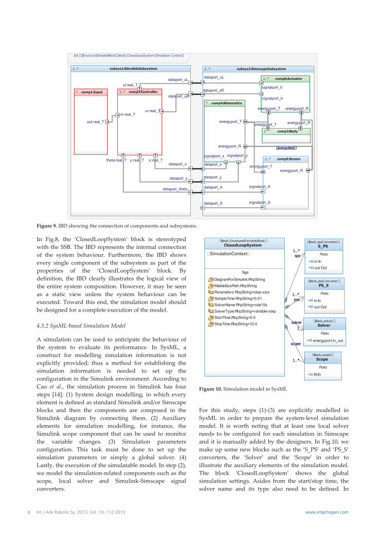
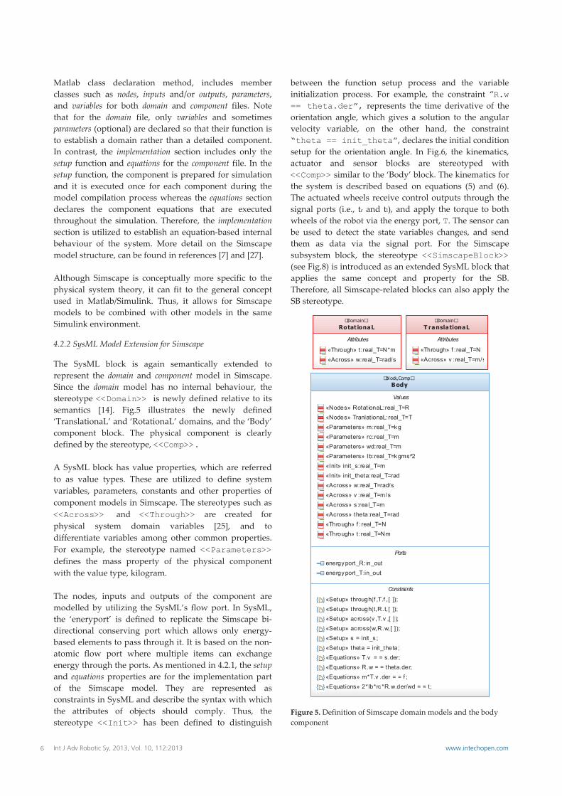
Figure 9. IBD showing the connection of components and subsystems.
In Fig.8, the ‘ClosedLoopSystem’ block is stereotyped with the SSB. The IBD represents the internal connection of the system behaviour. Furthermore, the IBD shows every single component of the subsystem as part of the properties of the ‘ClosedLoopSystem’ block. By definition, the IBD clearly illustrates the logical view of the entire system composition. However, it may be seen as a static view unless the system behaviour can be executed. Toward this end, the simulation model should be designed for a complete execution of the model. 4.3.2 SysML‐based Simulation Model
A simulation can be used to anticipate the behaviour of the system to evaluate its performance. In SysML, a construct for modelling simulation information is not explicitly provided; thus a method for establishing the simulation information is needed to set up the configuration in the Simulink environment. According to Cao et al., the simulation process in Simulink has four steps [14]: (1) System design modelling, in which every element is defined as standard Simulink and/or Simscape blocks and then the components are composed in the Simulink diagram by connecting them. (2) Auxiliary elements for simulation modelling, for instance, the Simulink scope component that can be used to monitor the variable changes. (3) Simulation parameters configuration. This task must be done to set up the simulation parameters or simply a global solver. (4) Lastly, the execution of the simulatable model. In step (2), we model the simulation‐related components such as the scope, local solver and Simulink‐Simscape signal converters.
Figure 10. Simulation model in SysML
For this study, steps (1)‐(3) are explicitly modelled in SysML in order to prepare the system‐level simulation model. It is worth noting that at least one local solver needs to be configured for each simulation in Simscape and it is manually added by the designers. In Fig.10, we make up some new blocks such as the ‘S_PS’ and ‘PS_S’ converters, the ‘Solver’ and the ‘Scope’ in order to illustrate the auxiliary elements of the simulation model. The block ‘ClosedLoopSystem’ shows the global simulation settings. Asides from the start/stop time, the solver name and its type also need to be defined. In
ibd [«StructuredSimulinkBlock» block] ClosedLoopSystem [Simulation Context]
subsys1:SimulinkSubsystem1..*
comp2:Controller1..*
in:real_Tur:real_T
ul:real_T
theta:real_T y:real_T x:real_T
comp1:Input*
out:real_T
dataport_theta
dataport_y
dataport_x
dataport_uR
dataport_uL
subsys2:SimscapeSubsystem1..*
comp6:Actuator1..*
signalport_tl
signalport_tr
energyport_T energyport_R
comp3:Body1
energyport_Renergyport_T
comp4:Kinematics*
energyport_T
energyport_R
signalport_x signalport_ycomp5:Sensor1..*
signalport_A
signalport_S
energyport_R
«energyBind»
energyport_T
dataport_y
dataport_x
dataport_S
dataport_A
dataport_uR
dataport_uL
«energyBind»
S_PS«block,spsC onv erter»
Ports
in:Inout:Out
PS_S«block,pssC onv erter»
Ports
in:Inout:Out
Scope«block,scope»
Ports
IN:In
Solver«block,solv er»
Ports
energyport:in_out
ClosedLoopSystem«block,StructuredSimulinkBlock»
::SimulationContext::
Tags
DiagramForSimulink:RhpStringMatlabExePath:RhpStringParameters:RhpString=step-sizeSampleTime:RhpString=0.01SolverName:RhpString=ode15sSolverType:RhpString=variable-stepStartTime:RhpString=0.0StopTime:RhpString=10.0
1..*sps
1..*pss
1solver
1..*
scope
1..*sps
1..*pss
1solver
1..*
scope
8 Int J Adv Robotic Sy, 2013, Vol. 10, 112:2013 www.intechopen.com
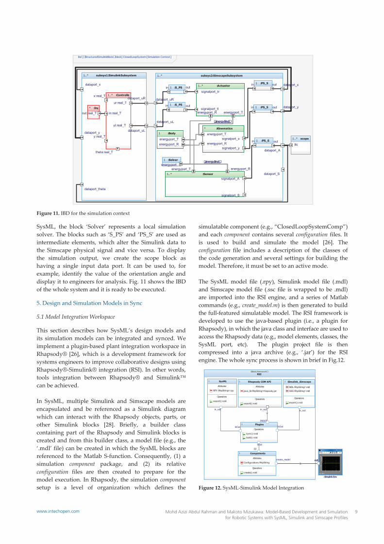
Figure 11. IBD for the simulation context
SysML, the block ‘Solver’ represents a local simulation solver. The blocks such as ‘S_PS’ and ‘PS_S’ are used as intermediate elements, which alter the Simulink data to the Simscape physical signal and vice versa. To display the simulation output, we create the scope block as having a single input data port. It can be used to, for example, identify the value of the orientation angle and display it to engineers for analysis. Fig. 11 shows the IBD of the whole system and it is ready to be executed.
5. Design and Simulation Models in Sync
5.1 Model Integration Workspace
This section describes how SysML’s design models and its simulation models can be integrated and synced. We implement a plugin‐based plant integration workspace in Rhapsody® [26], which is a development framework for systems engineers to improve collaborative designs using Rhapsody®‐Simulink® integration (RSI). In other words, tools integration between Rhapsody® and Simulink™ can be achieved. In SysML, multiple Simulink and Simscape models are encapsulated and be referenced as a Simulink diagram which can interact with the Rhapsody objects, parts, or other Simulink blocks [28]. Briefly, a builder class containing part of the Rhapsody and Simulink blocks is created and from this builder class, a model file (e.g., the ‘.mdl’ file) can be created in which the SysML blocks are referenced to the Matlab S‐function. Consequently, (1) a simulation component package, and (2) its relative configuration files are then created to prepare for the model execution. In Rhapsody, the simulation component setup is a level of organization which defines the
simulatable component (e.g., “ClosedLoopSystemComp”) and each component contains several configuration files. It is used to build and simulate the model [26]. The configuration file includes a description of the classes of the code generation and several settings for building the model. Therefore, it must be set to an active mode. The SysML model file (.rpy), Simulink model file (.mdl) and Simscape model file (.ssc file is wrapped to be .mdl) are imported into the RSI engine, and a series of Matlab commands (e.g., create_model.m) is then generated to build the full‐featured simulatable model. The RSI framework is developed to use the java‐based plugin (i.e., a plugin for Rhapsody), in which the java class and interface are used to access the Rhapsody data (e.g., model elements, classes, the SysML port, etc). The plugin project file is then compressed into a java archive (e.g., ‘.jar’) for the RSI engine. The whole sync process is shown in brief in Fig.12.
Figure 12. SysML‐Simulink Model Integration
ibd [«StructuredSimulinkBlock» block] ClosedLoopSystem [Simulation Context]
subsys1:SimulinkSubsystem1..*
:Controller1..*
in:real_T
ur:real_T
ul:real_T
theta:real_T
y:real_T
x:real_T
:Inp*
out:real_T
dataport_theta
dataport_y
dataport_x
dataport_uR
dataport_uL
subsys2:SimscapeSubsystem1..*
:Actuator1..*
signalport_tl
signalport_tr
energyport_Tenergyport_R
:Body1
energyport_Renergyport_T
:Kinematics*
energyport_T
«energyBind»
energyport_Rsignalport_x
signalport_y
:Sensor1..*
signalport_A
signalport_S
energyport_Renergyport_T
:PS_S1in out
:PS_S1in out
:PS_S1in out
:S_PS1in out
:Solver1
energyport«energyBind»
:S_PS1in out dataport_y
dataport_x
dataport_S
dataport_A
dataport_uR
dataport_uL «energyBind»
«energyBind»
scope1..*
IN
RSI«block,framework»
SysML1
Attributes
RPY:RhpString=.rpy
Operations
export():void
in_out
Simulink_Simscape1
MDL:RhpString=.mdlSSC:RhpString=.mdl
Operations
export():void
in_out
Rhapsody COM API1
Attributes
java_lib:RhpString=rhapsody.jar
Operations
export():void
in_out
Plugins1
Operations
sync():voidbuild():void
inout
INOUT
inOut InOut
Components1
Attributes
Configurations:RhpString
Operations
create():void
create_model
IO
mdl
:Simulink Env
mdl
:Simulink Env
9Mohd Azizi Abdul Rahman and Makoto Mizukawa: Model-Based Development and Simulation for Robotic Systems with SysML, Simulink and Simscape Profiles
www.intechopen.com

5.2 Implementation and Discussion
To validate our work, these models have to be executed in order to see if the system performs as expected. To this end, the system design model (see Fig.8) and the simulation model (see Fig.11) are evaluated. Once the model integration process is completed, the Simulink‐ and Simscape‐subsystem models can be generated by applying the ‘generate and simulate’ function available in the Rhapsody context menu. The execution process is shown in the Matlab command window and the generated model (e.g., “ClosedLoopSystem.mdl”) is auto‐simulated in the Simulink environment. If changes are made to the generated model, it will be automatically synced with the updated version. The generated model is depicted in Fig.13. In Fig.14, the simulation results are obtained for a simple system analysis. The results show a series of system responses to the robot orientation angle in setpoint when the robot mass is 3.76kg, and the desired input is set to (xd, yd, θd) = (0.25m, 0.25m, π/4rad). Simulation results in Fig.14 (a‐f) depict the orientation angle when parameters such as Ib, rc, wd, and rw were fixed to 0.01kgm2, 0.04m, 0.091m, and 0.032m respectively. The results demonstrate
output responses for a variety of controller coefficients tuning exercises. As for comparison, the controller can compensate the orientation error efficiently and settle to an acceptable setpoint in a short time. It should be borne in mind that the results are shown just to prove the practical use of our system‐level design framework and methodology. For more simulation and analysis, engineers have the option of manipulating other variables or parameters within the system.
Figure 13. Auto‐generated model in the Simulink window
Figure 14. Simulation results via scopes
(a) (b) (c)
(d) (e) (f)
10 Int J Adv Robotic Sy, 2013, Vol. 10, 112:2013 www.intechopen.com

6. Conclusion
In this paper, we attempted to develop a different perspective for system‐level design and simulation models especially for robotics by using the SysML (as the front‐end), Simulink and Simscape profiles. For this approach, the SysML design model and the Simulink/Simscape‐compatible models were created, synced and generated to carry out the simulation automatically. This preliminary effort can assist system designers and control engineers in collaborating as a team, from the first until the last of the development stages, in order to speed up the design and testing processes. In our method, the Simulink‐compatible model was first defined to represent the continuous‐time behaviour of the physical system. A method for extending the SysML semantics was then adopted to create a new set of stereotypes and their tagged values. This was done by extending the standard SysML block in conjunction with its behavioural model. We introduced the SB and SSB stereotypes to correspond to the standard Simulink block diagram and the Simulink environment respectively. Secondly, to enable an automatic simulation, we defined a SysML‐based simulation model for use in the Simulink environment. The simulation modelling approach has been proposed to model the simulation‐related components such as the signal converter, the local solver, the scope and the simulation parameters setting. Note that the physical system modelling is not a trivial matter because if the physical model is too concrete, then the simulation and design space exploration become expensive and it can even be difficult to detect problems. Therefore, an abstract model is more preferable during the conceptual stage of development; however abstraction of real physical systems needs deep understanding of the physical phenomenon [19]. For this study, we attempt to provide a specific SysML‐based model profile for the design and simulation of robotic systems. However, this paper considers only modelling and simulation works restricted to the MathWorks tools. In the future, we intend to evaluate our design models based on different modelling and simulation tools. Apart from that, we plan to integrate the system‐level design and analysis models using SysML’s parametric diagram for engineering analysis. At the time of writing this paper, we are in the process of developing a unified modelling framework for a comprehensive system and software design applicable to robotics, something which is considered rare.
7. Acknowledgments
The usage of Rational® Rhapsody® software is supported by the IBM® Academic Initiative collaboration program. The authors wish to express their gratitude to Hiroshi Ishikawa and Takashi Sakairi of IBM Research‐
Tokyo for their constructive comments and fruitful discussion. We also would like to thank Danai Phaoharuhansa and Prof. Akira Shimada who have helped in the technical discussion.
8. References
[1] C. Schlegel, A. Steck, D. Brugali and A. Knoll, “Design Abstraction and Processes in Robotics : From Code‐Driven to Model‐Driven Engineering,” Proceedings of Simulation, Modeling and Programming for Autonomous Robots (SIMPAR), Darmstadt, 2010, pp. 324‐335.
[2] J. Fisher, “Model‐Based Systems Engineering : A New Paradigm,” INCOSE Insight, vol. 1(3), pp. 3‐16, 1998.
[3] S.A. Friedenthal, “SysML: Lessons from Early Applications and Future Directions,” INCOSE Insight, vol. 12(4), pp. 10‐12, 2009.
[4] Object Management Group. (2010). Systems Modeling Language Specification. Available:
http://www.omg.org/spec/SysML/1.2/pdf/ [5] Object Management Group. (2010). Unified Modeling
Language Specification. Available: http://www.omg.org/spec/UML/2.3/pdf/ [6] T.A. Johnson, Integrating Models and Simulations of
Continuous Dynamic System Behaviour into SysML (Masters Dissertation of Georgia Institute of Technology). Atlanta: Georgia, 2008.
[7] MathWorks Inc. (2011). Simscape Language Fundamental. Available:
http://www.mathworks.com/help/toolbox/physmod/simscape/simscape_language.pdf/
[8] MathWorks Inc. (2011). Simulink. Available: http://www.mathworks.com/products/simulink/
[9] IBM Corporation. (2011). Rational® Rhapsody® Version 7.6. Available:
http://www.ibm.com/developerworks/rational/library/rhapsody_release‐v7.6/release.html/
[10] H. Bruyninckx, “Robotics Software : The Future Should Be Open,” IEEE Robotics & Automation Magazine, vol. 15(1), pp. 9‐11, 2008.
[11] S. Chhaniraya, C. Saaj, M. Althoff‐Kotzias, I. Ahrns and B. Maediger, “Model Based System Engineeing for Space Robotics Systems,” Proceedings of Symposium on Advanced Space Technologies in Robotics and Automation, Noordwijk, 2011.
[12]M.A. Abdul Rahman, et al., (2011). Model‐Driven Development of Intelligent Mobile Robot Using Systems Modeling Language (SysML). Mobile Robots ‐ Control Architectures, Bio‐Interfacing, Navigation, Multi Robot Motion Planning and Operator Training, Dr. Janusz Bȩdkowski (Ed.), ISBN: 978‐953‐307‐842‐7, InTech. Available: http://www.intechopen.com/books/mobile‐robots‐control‐architectures‐bio‐interfacing‐navigation‐multi‐robot‐motion‐planning‐and‐operator‐training/model‐driven‐development‐of‐intelligent‐mobile‐robot‐using‐systems‐modeling‐language‐sysml‐
11Mohd Azizi Abdul Rahman and Makoto Mizukawa: Model-Based Development and Simulation for Robotic Systems with SysML, Simulink and Simscape Profiles
www.intechopen.com

[13] K. Ohara, T. Takubo, Y. Mae and T. Arai, “SysML‐Based Robot System Design for Manipulation Tasks,” Proceedings of Intl. Conf. on Advanced Mechatronics, Osaka, 2010, pp. 522‐527.
[14] Y. Cao, Y. Liu and C.J.J. Paredis, “System‐Level Model Integration of Design and Simulation for Mechatronics Systems Based on SysML,” Mechatronics, vol. 21(6), pp. 1063‐1075, 2011.
[15] T.A. Johnson, C.J.J. Paredis, R. Burkhart and J.M. Jobe, “Modeling Continuous System Dynamics in SysML,” Proceedings of ASME Intl. Mechanical Engineering Congress and Exposition, Seattle, 2007, pp. 1‐9.
[16] T.A. Johnson, C.J.J. Paredis and R. Burkhart, “Integrating Models and Simulations of Continuous Dynamics into SysML,” Proceedings of Modelica Conf., Bielefeld, 2008.
[17] Modelica Association. (2011). Modelica Language. Available: http://www.modelica.org/
[18] Y. Venderperren and W. Dehaene, “From UML/SysML to Matlab/Simulink : Current State and Future Perspectives,” Proceedings of Design, Automation and Test in Europe (DATE) Conf., Munich, 2006.
[19] R. Kawahara, et al., “Verification of Embedded System’s Specification Using Collaborative Simulation of SysML and Simulink Models,” Proceedings of Second Intl. Conf. On Model Based Systems Engineering, Haifa, 2009, pp. 21‐28.
[20] S. Turki and T. Soriano, “A SysML Extension for Bond Graphs Support,” Proceedings of Fifth Intl. Conf. On Technology and Automation, Thessaloniki, 2005.
[21] K. Berkenköutter, S. Bisanz, U. Hannemann and J. Paleska, “HybridUML Profile for UML2.0,” Int J Softw Tools Technol Transfer, vol. 8(2), pp. 167‐176, 2006.
[22] S. Bensalem, F. Ingrand and J. Sifakis, “Autonomous Robot Software Design Challenge,” Proceedings of Sixth IARP‐IEEE/RAS‐EURON Joint Workshop on Technical Challenge for Dependable Robots in Human Environments, Pasadena, 2008.
[23] R. Siegwart, I.R. Nourbakhsh and D. Scaramuzza, Introduction to Autonomous Mobile Robots : Intelligent Robotics and Autonomous Agents series, 2nd Edition. Massachusetts: The MIT Press, 2009.
[24] J. Holt and S. Perry, SysML for Systems Engineering: Professional Applications of Computing series, 1st Edition. London: The IET, 2007.
[25] J.V. Amerongen and P. Breedveld, “Modeling of Physical Systems for The Design and Control of Mechatronic Systems : IFAC Professional Brief,” Annual Reviews in Control, vol. 27(1), pp. 87‐117, 2003.
[26] IBM Corporation. (2010). Rational® Rhapsody® User Guide. Available:
http://publib.boulder.ibm.com/infocenter/rsdp/v1r0m0/topic/com.ibm.help.download.rhapsody.doc/pdf75/UserGuide.pdf/
[27] MathWorks Inc. (2011). Simscape™ User’s Guide. Available: http://www.mathworks.com/help/pdf_doc/physmod/simscape/simscape_ug.pdf/
[28] X.H. Liu and Y.F. Cao, “Design of UAV Flight Control System Virtual Prototype Using Rhapsody and Simulink,” Proceedings of Intl. Conf. On Computer Design and Applications, Qinhuangdao, 2010.
12 Int J Adv Robotic Sy, 2013, Vol. 10, 112:2013 www.intechopen.com