Yves Thibaudeau

yves.thibaudeau@ccmail.census.gov

U.S. Bureau of the Census

Statistical Research Division

Research Report # RR-99-02

Model Explicit Item Imputation for Demographic Categories for Census 2000

1

Abstract

The paper shows results obtained when using a hierarchical log-linear model to produce item

imputations based on the maximum likelihood estimator. We compare the results with those

obtained using the sequential hot-deck imputation procedure. We apply the two procedures on the

data collected in Sacramento for the 1998 dress rehearsal for Census 2000. To measure the relative

differences between the two methodologies, we simulate the posterior and predictive distributions

associated with the model. We run our simulation through data augmentation bayesian iterative

proportional fitting (DABIPF). Gelman and Rubin (1991) first proposed a bayesian iterative

proportional fitting (BIPF) to generate posterior conjugates for categorical log-linear models. Schafer

(1997) proposes a variant of BIPF for direct application to hierarchical models. Schafer (1997) also

extends the technique to DABIPF. In our situation Schafer’s version of DABIPF yields: 1. An

approximation for the posterior distribution of the inclusion probabilities. 2. An approximation for

the predictive distribution of the population counts. The predictive distribution makes it possible to

give a full inferential assessment of the unreported population counts, and to compare our item

imputation procedure with the sequential hot-deck.

______________________________________________________________________________

Yves Thibaudeau, Mathematical Statistician, Statistical Research Division,

US Bureau of the Census, Room 3000-4, Washington, DC 20233-9100

yves.thibaudeau@ccmail.census.gov

2

Disclaimer

This paper reports the results of research and analysis undertaken by Census Bureau staff. It has

undergone a more limited review than official Census Bureau publications. This report is released

to inform interested parties of research and to encourage discussion.

3

1 Introduction

In the paper we set to develop and evaluate a model-based production-oriented procedure for item

imputation. We present our procedure as a competitor to the traditional hot-deck system at the

Bureau of the Census. To support and evaluate our item imputation procedure, and to compare it

with the hot-deck, we use a methodology developed in good part only in recent years. This

methodology is powerful. It provides us with the tools we need for our evaluation. Because this

evaluation methodology is relatively new, and some aspects of it were not entirely clear to us, we

felt necessary to include proofs for the assumptions we make in the paper. We attempt to motivate

our analysis in terms of its implications for the 1998 dress rehearsal in Sacramento, the example we

use as a test bed for our item imputation procedure.

In section 2 we introduce the example we will exploit for this research, the item imputation for the

1998 dress rehearsal of Census 2000 in Sacramento, and we recall the current methodology used for

this application. In subsection 2.1 we review a sample of the literature on the controversies

associated with bayesian item imputation. In subsection 2.2, we introduce the 1998 dress rehearsal

example. In subsection 2.3, we review the methodology of the Census Bureau to impute items

unreported during the dress rehearsal. In section 3 we present our tools for evaluating an imputation

methodology. Subsection 3.1 introduces the reference model and subsections 3.2 and 3.3 give a step

by step description of the data augmentation bayesian iterative proportional fitting (DABIPF)

procedure based on the model. DABIPF is the core of the evaluation machinery. Subsection 3.4 gives

examples of posterior and predictive distributions produced with DABIPF. These distributions serve

4

as gauges in the evaluation. In subsection 3.5 we propose an alternative procedure to produce item

imputations. In section 4 we present results on the item imputation for the 1998 dress rehearsal of

Census 2000 in Sacramento, and parallel results obtained with our alternative procedure. Subsection

4.1 gives interpretations for the predictive means and the predictive variances used to evaluate the

results. Subsection 4.2 gives values for the imputed counts, along with predictive means and

predictive standard deviations for several demographic categories. The results allow us in subsection

4.3 to evaluate the impact of the new Hispanic origin imputation methodology at the Census Bureau.

In subsection 4.4, we evaluate the relative bias of hot-deck item imputation with respect to the

model. In subsection 4.5, we analyze the performance of our alternative imputation procedure and

we compare it with that of the hot-deck. In section 5 we draw appropriate conclusions.

5

2 Background

2.1 Why Use Models for Item Imputation?

We intend to show that bayesian model-based inference can improve the quality of the imputation

of unreported items in censuses and demographic surveys. At the moment, the most common method

for demographic (categorical) item imputation is the hot-deck, either fixed-cell, sequential, or nearest

neighbor. It is particularly difficult to implement a hot-deck item imputation in a multivariate

context, because multivariate item imputation requires a careful elicitation of the dependencies

between items, and hot-deck specifications often fail to convey a complete representation of the

associations between the items. At the same time, we are aware that pitfalls in the deployment of

bayesian procedures involving item imputation have been reported. For instance, Fay (1996) gives

an instance where the variance of a t statistic is severely overestimated when using a particular

variance estimator based on bayesian multiple imputation. The estimator was proposed by Rubin

(1978, p. 76). In the same situation, the frequentist jackknife variance estimator based on hot-deck

imputation, which was proposed by Rao and Shao (1992), is nearly unbiased. Fay’s example reports

results for a situation where the bayesian estimator is used in a manner that is inconsistent with its

design. As such, this example is artificial, but it points to a legitimate concern, namely the

vulnerability of model-based methodologies to environments contrary to their underlying

assumptions. Although there is no way to ensure full protection against model mispecification, we

believe that the judgement of the analyst should ultimately help select a model adequately robust for

the survey it is intended.

6

Depending on the judgement of the analyst to select a model seems to us no more risky than

designing a multivariate hot-deck implemented through computer specifications. Analysts working

with models benefit from powerful analysis tools: the posterior and predictive distributions. To an

extent, we think that the separation between the professions of programmer and statistician, as

opposed to a profile integrating both occupations, makes it difficult to move away from using

computer specifications as the operational language in statistical institutions. We think computer

specifications are insufficient to thoroughly implement the process of statistical inference.

7

2.2 The 1998 Short Form

In March 1998 the Census Bureau conducted a dress rehearsal for Census 2000. Three sites were

targeted for the dress rehearsal: the city of Sacramento, a rural portion of South Carolina, and a

Menominee Indian reservation. The Sacramento test site is more diverse than the others, in terms of

race and Hispanic origin. We selected it to experiment with two item imputation procedures. Each

housing unit in Sacramento was sent a census questionnaire requesting at least six demographic

items for each occupant of the housing unit. The items were tenure, race, Hispanic origin, sex, and

age. A mail reply is expected from the household in each housing unit. Units for whom no mail reply

is received are the objects of a non-response follow-up operation, which included a sampling

procedure. After the data collection operations are completed, a substantial proportion (about 13 %)

of incomplete records remains. They correspond to units who did not provide all the demographic

items requested. Those items must be imputed.

The paper focuses on imputation of the household items. We define four household items

characterizing each household without ambiguity. The first household item is tenure, that is the home

ownership status of the household. The three other household items are defined through the

householder. They are race of the householder, Hispanic origin (origin) of the householder, and sex

of the householder. There is exactly one householder per household. Therefore, these items are

uniquely defined for each household. It is clear why tenure is considered a household item. There

are operational reasons for treating race and origin as household items. When race or origin are

unreported for an entire household, the values for the race or origin of the householder are imputed

8

through statistical procedures. Then, the values of the imputations carry to the other members of the

household. This procedure does not account for mixed households, but is a reasonable approximation

of the reality. Note that when race or origin are reported for at least one member of the household,

then the imputation is deterministic, in the sense that the unreported items are substituted with

reported items according to a predetermined hierarchy (1. substitute from the brother, 2. from the

mother, etc.). The sex of the householder seldom needs to be imputed. We include it among the

household variables because it interacts with them. We refer to Williams (1998) for a model-based

imputation procedure to impute age and to impute sex for household members other than the

householder. In the next subsection we review the imputation methodology that was used for the

dress rehearsal.

9

2.3 The Sequential Hot-Deck

The Census Bureau uses a sequential hot-deck (Kovar and Whitridge, 1995) to process the item-

imputation for the decennial census. Treat (1994) summarizes the specifications for the 1990

specifications. The sequential hot-deck (SHD) is essentially a one-pass algorithm. Except for a

preliminary initialization, the SHD processes the census records only once, and imputes any

unreported item on the spot by substituting the last recorded value for the item. In general, the

records are sorted according to geographical proximity, and thus the last record in the census file

usually corresponds to a near-by neighbor. In the 1998 version, additional constraints are imposed

on the SHD through the use of class variables (Treat, 1994). For example, race is a class variable for

origin. Accordingly, when a household does not report the origin item, it is borrowed from the last

household of the same race who reported origin. Subject matter experts are responsible for the

selection of the class variables. This version of the SHD is analogous to an unidirectional nearest

neighbor hot-deck. That is, the nearest neighbor always resides before the imputed record in the

order of the file.

Fay and Town (1998) suggest a rationale for relying on nearest neighbor algorithms. They mention

the concept of local exchangeability, which is akin to assumptions for some non-parametric

procedures. The exchangeability assumption certainly holds when the demographic composition of

a population is locally homogeneous with respect to geography. For example, we expect behavior

with respect to home ownership to be fairly homogeneous among neighbors. Race and origin also

exhibit a degree of local homogeneity. To the extent local homogeneity does not apply, the SHD

10

continues to borrow information from “nearest” neighbors, even though the rationale to support the

scheme has vanished. In the next section we propose an item imputation procedure based on

information retrieved at multiple levels of geography.

11

3 A Population Process

3.1 A Model for Population Counts

In order to develop an alternative item imputation procedure and to evaluate it, we design a model

representing a probabilistic population process at the level of a tract. A tract is a connected

geography of approximately 1700 households. The model channels information at three levels of

geography: the level of the household, the level of the neighbor, and the level of the tract. The

household provides information through the reported items. Neighbor and tract level information is

always available. Information about the neighbor and the tract is relevant for the purpose of item

imputation, since it gives a snap shot of the immediate and extended neighborhood surrounding the

household.

We establish the notation. For a given tract, let onmlkjiN be the population count for the households

with tenure i, race j, origin k, sex l, tenure of the neighbor m, race of the neighbor n, and origin of

the neighbor o. The notation for tenure is i = 1 if the unit of the household is owned, and i = 2 if it

is rented. The notation for race is j = 1 if the race of the householder is White, j = 2 if the race is

Black, j = 3 if the race is Asian, and j = 4 if the race is Other. The notation for origin is k = 1 if the

origin of the householder is non-Hispanic, and k = 2 if the origin is Hispanic. The notation for sex

is l = 1 if the sex of the householder is male, and l = 2 if the sex is female. The indices i, j, k, l

delineate 32 categories or cells for the households. We further characterize the households in terms

of the demographics of the neighbor. The “neighbor” in this case is the household preceding the

referenced household in the order of the census file. Census files are sorted by block. Blocks are

12

smaller connected geographical units. In urban settings, blocks correspond to the concept they

suggest. In general, consecutive blocks correspond to contiguous geographies. Thus the neighbor

usually lives in the same, or a neighboring block. The tenure of the neighbor is represented by m =

1 if the neighbor owns, and m = 2 if the neighbor rents. The race of the neighbor is given by n = 1

if the neighbor (householder) is non-Black, and n = 2 if the neighbor is Black. The origin of the

neighbor is defined by o = 1 if the neighbor is non-Hispanic, and o = 2 if the neighbor is Hispanic.

The notation distinguishes between 256 types of household for each tract.

Assume that M, the size of the population of households, is known for a given tract. Let onmlkjip be

the inclusion probability for type i, j, k, l, m, n, o, that is the probability that an arbitrary household

in the tract is of that type. Then, onmlkjiN , the set of counts for each household type, has a

multinomial distribution with M repetitions, and with probabilities onmlkjip . The likelihood

function is

(((( )))) (((( )))) onmlkjiN

onmlkjionmlkjionmlkjionmlkji ppNL ∏∏∏∏====; (1)

Initially, there is only one constraint imposed over the 256 inclusion probabilities onmlkjip . They

must be greater than zero and add-up to one. Our goal is to construct a meaningful model based on

a small number of key parameters. We want to keep the number of parameters small in part to

minimize the computer resources, but also because it permits information borrowing amongst the

estimates of the 256 inclusion probabilities. The following model integrates all two-way interactions

13

between household items and between respective items of neighbors.

(((( )))) (((( )))) (((( )))) (((( ))))(((( )))) (((( )))) (((( )))) (((( )))) (((( )))) (((( )))) oknjmilkljkj

likijionmlkjionmlkji

HRTSHSRHRSTHTRTSHRTp

ηρτηρτµ

*********log

++++++++++++++++++++++++

++++++++++++++++++++++++++++++++++++++++==== (2)

The log-linear parameters with one subscript represent the main effects corresponding to the items

identified by the subscript. The log-linear parameters with two subscripts represent the interactions

between the two items identified by the subscripts. To prevent redundancies, we set the following

constraints:

(((( )))) (((( )))) (((( )))) (((( )))) (((( )))) (((( ))))

(((( )))) (((( )))) (((( )))) (((( )))) (((( )))) (((( ))))

(((( )))) (((( )))) (((( )))) (((( )))) (((( )))) (((( )))) 0******

0******

0******

0

========================

========================

========================

============================

kok

jnj

imi

ook

nnj

mmi

llk

llj

kkj

lli

kki

jji

klk

jlj

jkj

ili

iki

iji

oo

nn

mm

ll

kk

jj

ii

HRTHRT

SHSRHRSTHTRT

SHSRHRSTHTRT

SHRT

ηρτηρτ

ηρτ

(3)

We will represent the statement that the inclusion probabilities jointly satisfy the constraint

1,,,,,,

====onmlkji

onmlkjip , the constraints in (2), and the constraints in (3) by

Θ∈∈∈∈onmlkjip (4)

The architecture of the log-linear model defined in (2) is inspired from the same concepts motivating

the SHD, since the model includes interaction effects between the items of neighboring households.

14

3.2 Simulating the Parameters through Bayesian Iterative Proportional Fitting

The bayesian approach puts unreported items and parameters on a par. Both need to be simulated

to produce measures that we can use to evaluate the SHD and prospective competing procedures.

In this subsection we set-up the stochastic environment for the parameters. In the next subsection,

we present the simulation of unreported items. To stochastically describe the parameters we identify

a conjugate family of prior and posterior distributions. A natural choice for a conjugate family is to

set the density of a member of the family to be of the same form as the likelihood. In that spirit,

Schafer (1997, p. 306) defines the constrained dirichlet conjugate family. The corresponding density

defines a probability distribution on the inclusion probabilities onmlkjip . The density of a general

member of the constrained dirichlet family is

(((( )))) (((( )))) (((( ))))

Θ∈∈∈∈

==== −−−−∏∏∏∏

onmlkji

onmlkionmlkjionmlkjionmlkjionmlkji

p

pCpf onmlkji 1ααα

(5)

(((( ))))onmlkjiC α is the integration constant, and onmlkjiα are the characteristic hyperparameters of a

member of the constrained dirichlet family. Θ is defined in (4). We have 0>>>>onmlkjiα , for all

values of the subscripts. We state a fact that will give us a stochastic environment to simulate the

inclusion probabilities onmlkjip when the density is of the form in (5). The proof follows directly

from the definition of the likelihood in (1), and the density in (5) (DeGroot, 1970, p.174).

15

Fact 1: If onmlkjip has the prior density in (5), then, given the likelihood in (1) and (4), the

posterior density of onmlkjip after observing onmlkjiN is defined by replacing onmlkjiα with

*onmlkjiα in (5), where onmlkjionmlkjionmlkji N++++==== αα * .

Fact 1 gives a characterization of the posterior distribution in terms of the density in (5), and thus

the constrained dirichlet is a genuine conjugate family. However, because of the constraint in (4),

the constrained dirichlet is intractable, that is (((( ))))onmlkjiC α in (5) is unavailable algebraicaly. Tierney

and Kadane (1986) present applications of the method of Laplace to approximate the posterior

moments of intractable distributions. Thibaudeau (1988) extends the method to multimodal posterior

distributions. We expect approximations obtained with the method of Laplace to be accurate in the

present situation, given the large sample size. The drawback is the amount of analytical work needed

to apply the method for the model in (2). In this situation, the method involves the computation of

the hessian for the twenty-six parameters in (2). An available alternative is to let the computer do

all the work. Gelman and Rubin (1991) propose an algorithm, bayesian iterative proportional fitting

(BIPF), to simulate the parameters of a log-linear model. The algorithm is based on a conjugate

family associated with the product of gamma densities. Schafer (1997, p. 308) adapts BIPF to our

situation, that is to simulate the parameters of the constrained dirichlet conjugate family. In our

situation, Schafer’s version of BIPF involves nine simple parameterizations. They correspond to the

following nine sets of joint marginal inclusion probabilities.

16

,,,,

,,,,,

oknjmilk

ljkjlikiji

pppp

ppppp

++++++++++++++++++++++++++++++++++++++++++++++++++++++++++++++++++++++++++++++++

++++++++++++++++++++++++++++++++++++++++++++++++++++++++++++++++++++++++++++++++++++++++++++++++++++ (6)

To produce a valid simulation of the density in (5) using BIPF, we need two additional facts. These

facts apply to the parameterizations in (6). We state them in terms of the first set in (6),

corresponding to tenure and race, but analogous facts hold for the other sets. We include a proof of

facts 2 and 3 in Appendix A.

Fact 2: If onmlkjip has the distribution given in (5), then, conditional on the set of conditional

inclusion probabilities

++++++++++++++++++++ji

onmlkji

pp , the distribution of ++++++++++++++++++++jip is an unconstrained

dirichlet with posterior parameters given by onmlkjionmlkjionmlkji N++++==== αα * , with the density

(((( ))))

1;4,3,2,1;2,1;0

,,

4,3,2,12,1

1

4,,12,1

*

============>>>>

∝∝∝∝

∏∏∏∏

========

++++++++++++++++++++++++++++++++++++++++

−−−−

========

++++++++++++++++++++++++++++++++++++++++

++++++++++++++++++++++++++++++++++++++++

ji

jiji

ji

jionmlkjionmlkjiji

onmlkjiji

pjip

pNpp

pf jiαα

(7)

Fact 3: ++++++++++++++++++++jip and

++++++++++++++++++++ji

onmlkji

pp are statistically independent.

17

Fact 3 follows directly from fact 2, since neither the functional on the RHS of (7), nor the range of

++++++++++++++++++++jip in (7), involve

++++++++++++++++++++ji

onmlkji

pp . The three facts in this subsection are sufficient to

validate a simulation of (5) through BIPF. We detail one cycle of the BIPF algorithm. For now, we

assume that the algorithm has been running, and has produced at least one value for onmlkjip ,

according to (5). We discuss choosing a starting point in the next subsection. The steps below

describe the cycle of BIPF involving the set of marginal inclusion probabilities ++++++++++++++++++++jip

corresponding to tenure and race. The cycles corresponding to the other sets in (6) are similar.

Step 1

Generate newjip ++++++++++++++++++++ , as follows:

- Compute ++++++++++++++++++++jiN the marginal counts corresponding to tenure and race.

- Generate eight gamma random variables 422111 ,,, GGG with scale parameters

++++++++++++++++++++++++++++++++++++++++++++++++++++++++++++++++++++++++++++++++ ++++++++ 42421111 ,, αα NN , where onmlkjiα is the set of prior

hyperparameters.

-++++++++

====++++++++++++++++++++ G

Gp jinewji

, yields the new simulation of ++++++++++++++++++++jip , which has the unconstrained

dirichlet in (7).

18

Step 2

Update the inclusion probabilities through the formula:

====

++++++++++++++++++++++++++++++++++++++++

ji

onmlkjiji p

ppp newnew

onmlkji (8)

BIPF then repeats steps 1 and 2 to update onmlkjip with respect to the other sets of joint marginals

in (6). When all nine sets of joint marginals have been generated, repeat the nine types of cycle. BIPF

simulates the density function given in (5). Schafer (1997, p. 315) gives a heuristic argument for the

convergence of the BIPF algorithm described above, but does not mention fact 3, independence,

which is necessary. We include a proof of convergence in appendix B.

19

3.3 Simulating the Parameters and the Unreported Items

Our ultimate goal is the evaluation of the SHD and of our competing item imputation procedure,

which we introduce in subsection 3.5. The tool we need for this evaluation was partly defined in the

preceding subsection. In this subsection we include material that allows us to define a fully

functional evaluation tool. This tool is the predictive distribution connected to the model in (2). The

predictive distribution will allow us to assess the compatibility of the model with an arbitrary item

imputation procedure. To simulate the predictive distribution, Schafer (1997, p. 324) further extends

BIPF to data augmentation iterative proportional fitting (DABIPF). DABIPF is a cross between

BIPF, and the data augmentation algorithm of Tanner and Wong (1986). DABIPF is designed to

generate a Markov chain Monte-Carlo (MCMC), which simulates both the inclusion probabilities

onmlkjip and the unreported items of the population process. DABIPF consists of cycling through

the following two steps:

I Step Conditional on the current inclusion probabilities onmlkjip , impute the unreported items

for each household and update the population counts onmlkjiN .

P Step Conditional on the population counts onmlkjiN , generate a new value for the inclusion

probabilities onmlkjip through a cycle of BIPF.

At each cycle, the P step generates the values of a set of joint marginal inclusion probabilities in (6),

20

as explained in the previous subsection for BIPF. It takes nine I steps, each followed by a P step,

before the inclusion probabilities onmlkjip are updated with respect to each set of joint marginal

probabilities in (6). Before explaining how DABIPF works, we take care of some unfinished

business: the starting point. For both BIPF and DABIPF, an initial value for onmlkjip is needed to

initiate the algorithm. This value must satisfy (4). A sure candidate for the initial value is obtained

by setting the inclusion probabilities equal to each other. Given the initial value, the I step is carried

by simulating a multinomial distribution based on the imputation probabilities. We illustrate the I

step in the situation where only origin may be unreported. It is easily generalized to situations

involving any number of unreported items. Let onmlji ++++Λ represents the observed count of households

with known value for the items corresponding to i, j, l, m, n, o, but with unreported origin. To carry

the I step we compute the imputation probabilities from the current inclusion probabilities with the

standard formula

2,1;21

====++++

====++++ kpp

p

onmljionmlji

onmlkjikonmljiΨ (9)

We impute origin for each of the onmlji ++++Λ households by flipping a coin with probability 1onmlji ++++Ψ

of a tail landing, and probability 2onmlji ++++Ψ of a head landing. If the actual landing is a tail, we

substitute “non-Hispanic” for the unreported origin of the household, if the landing is a head, we

substitute “Hispanic” for the unreported origin.

After going through the I step, we have a full set of population counts defined by the observations

21

and the imputations. Then, DABIPF updates onmlkjip through the P step, as described for BIPF.

After a burn-in period, the DABIPF algorithm reaches its stationary distribution. The stationary

posterior distribution is a finite mixture of constrained dirichlet distributions as given in (5). We give

examples of posterior distributions in the next subsection.

The convergence of DABIPF to the posterior distribution in (5) follows from two facts: 1. The

convergence of the data augmentation algorithm. 2. The convergence of BIPF. In appendix B we

define the properties of invariance and irreducibility, which guarantee convergence. We can check

that the invariance property holds for DABIPF, through the data augmentation equations (Tanner and

Wong, 1986). Let OkjiN represent the observed count for tenure, race, and origin i, j, k, where the

subscripts take the value 0, when the corresponding item is misssing, and let U represent the

information on the unreported items. The data augmentation equations are:

(((( )))) (((( )))) (((( )))) (((( ))))

(((( )))) (((( )))) (((( )))) (((( ))))====

====

kjiO

kjikjiO

kjikjikji

Okji

Okjikji

Okjikji

pdNpfNpUfpUf

UdNUfUNpfNpf

,

,

(10)

The first integral represents the P step: DABIPF generates a new value for kjip from the posterior

density (((( ))))UNpf Okjikji , , obtained by completing the observed data with a simulated value for

U. The second integral represents the I step: DABIPF generates a new value for U from the

22

predictive distribution (((( ))))Okjikji NpUf , , obtained through a simulation of kjip . Since both the

P and I steps draw simulated values from the correct posterior and predictive distributions, the

MCMC remains consistent with the original posterior and predictive at each cycle. This implies that

the MCMC is invariant. The irreducibility property follows from the irreducibililty of BIPF, and the

nature of the multinomial distribution. In the next subsection we give simulation results based on

the 1998 dress rehearsal.

23

3.4 The Posterior Distribution for Tract X

We give illustrations of the posterior distribution, as approximated through 5454 cycles of DABIPF

for tract “X” from the Sacramento site. We deleted the initial 54 cyles, as DABIPF stabilizes during

those initial cycles. The tract contains 1583 households and exhibits typical patterns for a mixed race

and mixed origin neighborhood. The posterior distribution represents our knowledge of the

parameters of the model in (2), after observing the data and helps us understand the interactions at

work in the data.

Tract X has four non-Hispanic female renters who did not report their race and who have a non-

Black non-Hispanic renter for neighbor. Figure 1A shows the approximation for the posterior

distribution of 112212

1122122

++++pp , which is the probability a householder with these characteristics is

black. In tract X, there are also four householders who did not report race and are in the same

situation as the previous four, except that their neighbor is Black. Figure 1B shows the

approximation for the posterior of 122212

1222122

++++pp , the probability that a householder is black given

it exhibits the characteristics of the second group. The contrast between figures 1A and 1B reflects

the effects of the race of the neighbor (non-Black, Black) on the race of a household, in probabilistic

terms.

Figures 2A and 2B illustrate another contrast. Tract X has two male non-Hispanic Asian

householders with non-Black non-Hispanic renters for neighbors, and two male non-Hispanic Black

24

householders with non-Black non-Hispanic renters for neighbors. These four householders did not

report tenure. Figures 2A and 2B show the posterior distributions of 112112

1121121

++++pp and

112113

1121131

++++pp , the probabilities of owning a home, for a householder in the first and second pair

respectively. The contrast between the two posterior distributions illustrates the effect of race on the

probability of home ownership. It is clear that the probability of ownership is higher for Asians than

it is for Blacks. But our knowledge for the Asians is less decisive than for the Blacks, that is the

posterior in 2A is flatter. The contrast between 2A and 2B is an illustration of the interaction

between tenure and race. We investigate the implications of this interaction in the next section. In

particular we assess the discriminatory power of the SHD in reflecting this interaction through the

imputed data.

The posterior distribution is a powerfull analytical instrument and can be used to elicit an appropriate

model for item impuation. However, if we have sufficient confidence in the design of the model, we

want to begin the production activity and we do not need analytical feed-back at every stage of the

production process. In this context, we would like an efficient procedure, which produces item

imputations consistent with the model. We present a procedure of that type in the next subsection.

25

26

3.5 A Production-Oriented Imputation Procedure

In a production environment, if we assume that a reasonable model has been delineated, we can

generate a single round of item imputation within a reasonably short period of time. We propose

generating item imputations conditional on the maximum likelihood estimator (MLE) of the

imputation probabilities. Thibaudeau et Al. (1997) give results using this procedure, but without

error estimates. Zanutto and Zaslavsky (1997) use a similar technique, but they eliminate much of

the noise of the simulation by contriving the imputed population counts to be equal to an estimate,

rounded-off to the nearest integer. Reducing the synthetic noise leads to estimates that are near

optimal. We suggest an alternative way to achieve that goal at the end of this subsection. However,

for our present analysis, we do not attempt to control the noise associated with the simulation,

because for this example, we think that it is negligible. We will see in the next section that the noise

of the simulation and the variance are dwarfed by the size of some biases, at the level of Sacramento.

Our production-oriented item imputation procedure makes use of the EM algorithm (Dempster,

Laird, and Rubin, 1977). The steps of our procedure are:

- For each tract, through the EM algorithm evaluate onmlkjip the maximum likelihood

estimator (MLE) of onmlkjip based on the model in (2).

- From onmlkjip , compute konmlji ++++Ψ , the MLE’s of the imputation probabilities k

onmlji ++++Ψ

27

computed in (9). When items other than origin are missing, the formula in (9) is adapted.

- Use the imputation probabilities with a multinomial random generator to produce an

imputation for the unreported items.

This procedure is compatible with a production environment in terms of time and other resources.

The M step of the EM algorithm can be implemented with a standard iterative proportional fitting

routine, such as “CATMOD” in SAS. A multinomial random generator, such as “RANTBL” in SAS,

is needed to generate the unreported items based on the MLE of the imputation probabilities. To

control the simulation noise, a possible strategy is to repeat the last step of our procedure several

times, and take the imputation yielding the population counts closest to the MLE, according to some

metric. We give a full evaluation of the error associated with our procedure outlined in subsection

4.5.

28

4 Results for Model-Based Imputation and the Sequential Hot-Deck

In this section we present the reported results for the item imputation for the 1998 dress rehearsal

of Census 2000 in Sacramento, along with an approximation of the predictive distribution obtained

through DABIPF, and results for our production-oriented procedure of subsection 3.5. We had no

input in the design or the implementation of the SHD used to produce the item imputations reported

for the dress rehearsal. We conducted our research from files made available to us by the staff of the

Decennial Management Division at the Census Bureau, after completion of the edit and imputation

phase of the dress rehearsal, in January1999.

Our analysis is somewhat over-simplified as we exclude from it all the vacant housing-units. We also

ignore the additional error created by the sampling for non-response operations that created virtual

housing units amounting to about 2 % of all units in Sacramento. These sources of error can certainly

be integrated in a more comprehensive model, but at this time we focus on evaluating the item

imputation procedure while controlling for other effects.

29

4.1 Bayesian Measurements and Format of the Results

We begin this section with a review of our evaluation tool, the predictive distribution. We will use

this tool to evaluate the counts produced with the SHD, and the counts obtained with our production-

oriented procedure. For the remaining analysis, we drop the subscripts in the notation for the

population count onmlkjiN , which we denote by N. A specific type of population will be defined

explicitely if need be. We represent the entirety of the observations collected for the dress rehearsal

by Ω . With that notation, the predictive mean and predictive variance of N are [[[[ ]]]]ΩNE and

[[[[ ]]]]ΩNV respectively. Let zN represent the population counts generated at the z-th cycle of

DABIPF. Then we can approximate the predicitive mean and predictive variance through

[[[[ ]]]] [[[[ ]]]][[[[ ]]]](((( ))))

Z

NENNV

Z

NNE

Z

z

zZ

z

z

========−−−−

≈≈≈≈≈≈≈≈ 1

2

1 ;Ω

ΩΩ (11)

These approximations are exact when Z, the number of DABIPF iterations, goes to infinity.

Asymptotically in terms of sample size, or tract size here, the predictive mean equivalent to the

maximum likelihood estimator (MLE) of the expectation of the population counts, conditional on

the observations. Regardless of the convergence properties, the predictive mean is an optimal

decision for the value of the population counts, under quadratic loss (DeGroot, 1970, p.228).

In Table 1 we give values obtained through DABIPF for the predictive means and predictive

standard deviations of the population counts for 28 demographic categories. These values are

30

approximations based on two implementations of DABIPF. We also give in table 1, two instances

of imputations produced with our production-oriented imputation procedure of subsection 3.5, along

with the corresponding reported counts (SHD). Each implementation of DABIPF generates 1800

cycles, for each of the 108 tracts in Sacramento. For each tract, the prior hyperparameters are set

according to onmlkjiα = .01, in the prior distribution given by (5). Our intent is to have a posterior that

is nearly identical to the likelihood. We discarded the generated counts and parameters for a burn-in

period of 54 cycles for each implementation. We eyeballed through graphs of the population counts

across cycles and the approximated predictive distribution appears stable. DABIPF stabilizes rapidly

since it draws values from the exact posterior distribution, conditional on the last round of

imputations, and less than 15% of the households are missing any item. In the tables, we used the

formula in (11) to approximate the predictive mean. For the variance, to avoid induced correlations

between the values of N in virtue of their contribution to the sample mean, we divided the data in

ten groups of 180 realizations of the population counts. Each realization is separated from the next

one in the same group by a lag of ten cycles of DABIPF. We took the sample variance for each group

and then averaged the ten variances to get an estimate of the predictive variance. The standard

deviations presented in the tables of this section are the square-root of those variances. It turns out

that the results are almost identical to those we get if we blindly apply the variance formula in (11).

We programmed DABIPF in SAS, using the multinomial generator “RANTBL” and the gamma

generator “RANGAM”. The original data file for Sacramento is about seventy megabytes. Each 1800

cycles implementation takes approximately twelve hours in CPU cycles on a SUN SPARC,

generating about one-half gigabyte of data each. The output file in each case is a record of the

31

household counts, for each pattern of reported and unreported items at each cycle. The counts are

added over all tracts, for each pattern. We had SAS write all the intermediary files in a cache (/tmp),

while the counts were accumulated on hard disk, at each cycle. This scheme resulted in a wall time

practically equal to the CPU time.

32

Table 1 Sequential Hot-Deck vs. Quick Imputation and Two Predictive Distributions

Population Reported

Count:

SHD

And

Dictionary

Production

Oriented

Imputation

Adjusted

for Diction.

DI

Production

Oriented

Imputation

I

Predictive

Mean

Adjusted

for the

Dictionary

[ ]ΩDNE

Predictive

S. D.

Adjusted

for the

Dictionary

[ ]ΩDNV

Predictive

Mean

[ ]ΩNE

Predictive

S. D.

[ ]ΩNV

All 138271 138271 138271 138271 0 138271 0

White 89032 88890 88876 88927.1 36.3 88930.3 35.5

Black 19962 19937 19979 19957.0 15.6 19953.9 16.1

Asian 17405 17423 17439 17426.6 14.8 17427.1 15.2

Other 11872 12021 11977 11960.3 35.3 11959.8 32.8

Non-His. 117247 117221 117127 117232.3 10.3 117126.1 17.3

Hispanic 21024 21050 21144 21038.7 10.3 21144.9 17.3

White NH 79964 79936 79854 79934.8 15.6 79864.6 19.0

White His. 9068 8954 9022 8989.3 34.8 9065.6 35.9

Black NH 19357 19328 19344 19345.1 10.6 19335.0 11.8

33

Black His. 605 609 635 611.9 12.5 618.9 14.1

Asian NH. 16887 16911 16901 16909.8 10.1 16895.4 11.1

Asian His. 518 512 538 516.8 11.5 531.6 12.6

Other NH. 1039 1046 1028 1042.7 3.5 1031.1 3.9

Other His. 10833 10975 10949 10917.6 34.3 10928.7 33.0

Owner 70054 70064 70056 70021.7 42.6 70022.8 43.2

Renter 68217 68207 68215 68249.3 42.6 68248.2 43.2

White O. 47722 47776 47778 47770.8 40.6 47776.1 41.0

White R. 41310 41114 41098 41156.3 40.9 41154.1 42.1

Black O. 7661 7576 7543 7540.7 20.9 7538.7 20.2

Black R. 12301 12361 12436 12416.3 21.8 12415.2 22.3

Asian O. 9810 9848 9880 9874.1 19.0 9874.9 19.0

Asian R. 7595 7575 7559 7552.5 18.1 7552.2 19.0

Other O. 4861 4864 4855 4836.2 26.7 4833.1 26.7

Other R. 7011 7157 7122 7124.1 28.8 7126.7 29.1

NH Owner 60645 60676 60576 60615.4 38.7 60559.4 40.1

NH Renter 56602 56545 56551 56617.0 39.1 56566.7 40.3

His. Owner 9409 9388 9480 9406.3 20.3 9463.4 23.0

His. Renter 11615 11662 11664 11632.3 20.7 11681.4 23.3

34

4.2 Adjustment for the Dictionary of Hispanic Last Names

When setting-up our production-oriented procedure in subsection 3.5, we clearly intended it as a

competitor for the SHD. To give a thorough comparative evaluation between our procedure and the

SHD, in terms of population count, we must control for relative biases that are not artifacts of the

methodological differences between the two procedures. In 1998, the Census Bureau developed a

dictionary of last names to determine origin when unreported. The dictionary is site based. In

Sacramento, out of 3934 households with unreported origin, 2604 had origin imputed through the

dictionary. This means that, relative to the origin of last names in the Sacramento area, their last

names had strong Hispanic, or strong non-Hispanic affiliations. The remaining 1330 households had

their origin imputed with the SHD. To assess and adjust for the effect of the dictionary, we

implemented two versions of DABIPF. For the first version, we ignore the imputations obtained

through the dictionary and we assume that no information is available on the origin of the 3934

households who did not report it. Table 1 gives the predictive means and predictive standard

deviations under this assumption. For the second version, we respect the imputation of origin based

on the dictionary. In this case, we assume that only the 1330 households who were not assigned

origin through the dictionary did not report it. Table 1 gives the predictive means and standard

deviations under this assumption. Table 1 also gives population counts obtained through two runs

of our production-oriented imputation procedure described in subsection 3.5, the first run ignoring

the last name dictionary, and the second run respecting it. We give the results along with the reported

counts for the 1998 dress rehearsal. The reported counts were obtained with the SHD and the

dictionary. We refer to the values respecting the decision of the dictionary as being “adjusted for the

35

dictionary”. In the next subsection we use the two versions of the predictive to assess the impact of

the dictionary, and evaluate the SHD.

36

4.3 Imputation of Hispanic Origin with the Dictionary of Hispanic Last Names

We use the results from DABIPF to assess the magnitude of the effect of the dictionary of Hispanic

last names, and account for this effect in our evaluation of the SHD. Ideally, we would use an

evaluation methodology of the type discussed by Gelman and Meng (1996, p. 192). The scheme

proposed by the authors is the progressive evaluation of a model through its expansion. This allows

the statistician to formally update his/her posterior opinion after introducing a new variable, or a new

interaction. Unfortunately, we face a “fait accompli”. We do not have the information we need to

enrich our model. We have an indicator corresponding to each household whose origin is imputed.

The indicator simply records whether the SHD, or the dictionary of Hispanic last names is the source

of the imputation for origin. We do not have information on the decision of the dictionary regarding

the origin of households who reported it.

To assess the impact of the dictionary, and evaluate the SHD, we resort to a simplistic strategy. First

we evaluate the relative distance between the reported population counts, and the predictive mean

counts [[[[ ]]]]ΩNE , under the model in (2). Then we repeat the evaluation, but this time we compare

the reported counts with [[[[ ]]]]ΩDNE , the predictive mean counts adjusted for the dictionary. We

assess the distance between the reported count and the predictive mean count in terms of the

predictive standard deviation [ ]ΩNV , and the predictive standard deviation adjusted for the

dictionary [[[[ ]]]]ΩDNV , respectively. The contrast between the two distances determines our

assessment of the impact of the dictionary.

37

Naturally, we first look at the population count for Hispanic households. We observe that the

distance between the predictive mean count ( [[[[ ]]]]ΩNE = 21144.9) and the reported count of

Hispanics (21024) is more than six standard deviations ( [[[[ ]]]]ΩNV = 17.3 ), indicating a serious

conflict between the model and the reported count. On the other hand, the distance between the

adjusted predictive mean count ( [[[[ ]]]]ΩDNE = 21038.7) and the reported count is moderate in terms

of the standard deviation ( [[[[ ]]]]ΩDNV = 10.3). In this case the impact of the dictionary is very

substantial. Table 1 reveals many conflicts between the reported count and the predictive mean for

the categories involving origin. However, the adjustment for the dictionary resolves most of the

conflicts. Because the adjustment lowers the predictive mean for Hispanics, the data suggests that

the dictionary is deflecting a bias confounded with the value of the origin item. It appears that non-

Hispanic households do not report origin in part because they are not Hispanic. Additional

investigation is needed to confirm this hypothesis, but if it holds, the dictionary methodology is a

breakthrough. The staff of the Population Division of the Census Bureau is responsible for the design

of the dictionary of Hispanic last names. In the next subsection, we examine a situation where the

reported count and the predictive mean are in conflict despite the adjustment for the dictionary.

38

4.4 Imputation of Tenure for Black Households

Table 1 reveals a sizable discrepancy between the predictive mean ( [[[[ ]]]]ΩNE = 7538.7) for the

population count of Black owners, and the reported count (7661), in terms of the predictive standard

deviation ( [[[[ ]]]]ΩNE = 20.2). The situation is not alleviated by the adjustment for the dictionary

of Hispanic last names. In an attempt to explain the conflict, we compare the rate of ownership for

Blacks with the rate of ownership of their neighbors. Our rationale for this comparison comes from

the design of the SHD. When tenure is unreported, the SHD borrows it from the neighbor,

accounting for only one class variable, in this case, household size. We compute the means and

variances for the rates of ownership for Blacks from the predictive distribution. Note that we need

not be concerned about transforming the variables from counts to ratios.

In table 2 we observe that the reported rate of ownership for Blacks with imputed tenure (.436) is

larger than the rate of ownership for Blacks with reported tenure (.379). At the same time, the rate

of ownership for Blacks with imputed tenure is close to that of their neighbors (.419). This reflects

the strategy of the SHD: replicate the tenure of the neighbor, borrowing the items from the nearest

neighbor with a similar household size. This strategy does not adjust for race. On the other hand, the

predictive mean of the rate of ownership for Blacks with imputed tenure (.375) is in agreement with

the rate of ownership for Blacks with reported tenure. The conflict is serious. The SHD produced

a rate of ownership more than five standards deviations (.0104) above the predictive mean rate for

Blacks with imputed tenure.

39

The data imply that, overall, Black households own a home less frequently than their neighbors do.

About 5% less often, relative to the size of the Black population. Imputation through the SHD blurs

the interaction between race and tenure. We think that this discrepancy is typical of the SHD. One

could argue that an additional class variable or a different sort order could solve the problem. But

almost invariably, some multivariate dependencies get lost somewhere along the specification

process.

40

Table 2 - Rates of Ownership for Black Households in Sacramento

Household

Type

Number of

Black

Households

Ownership

of the

Neighbors

Ownership

for the

Households

with

Reported

Tenure

Ownership

for the

Households

with Imputed

Tenure

(SHD)

Predictive

Mean

Rate of

Ownership

Predictive

S.D. of

the Rate of

Ownership

Tenure

Reported 18176 .428 .379 N /A .378 .00035

Tenure

Unreported 1786 .419 N /A .436 .375 .010

41

4.5 Error Analysis for the production-oriented Imputation Procedure

In this subsection we give a full evaluation of the error associated with our production-oriented

imputation procedure presented in subsection 3.5. A realization of the imputed population count I,

simulated with our procedure based on model (2), is given in table1. A second realization, DI , is

given in table 1, and corresponds to an implementation of our procedure based on model (2) and

adjusted for the dictionary of Hispanic last names. To evaluate the error involved when estimating

the true population count N with I, we must account for two types of uncertainty. First, the

uncertainty associated with the population process, as described by the model in (2). Second, the

uncertainty associated with I, the outcome of our “coin flip” based on the value of onmlkjip , the

MLE of the inclusion probabilities. Our knowledge and our level of uncertainty regarding N is

represented by the predictive distribution approximated through DABIPF. The second uncertainty

is synthetic. It is the noise associated with a multinomial random variable with constant probabilities

onmlkjip . A measure of the total error associated with guessing N through I is the square root of the

mean squared error:

SQMSE = (((( ))))[[[[ ]]]] [[[[ ]]]] [[[[ ]]]](((( )))) [[[[ ]]]] [[[[ ]]]]ΩΩΩΩΩ NVIVNEIEINE ++++++++−−−−====−−−−22

[[[[ ]]]] [[[[ ]]]]ΩΩ NEIE −−−− is the estimation bias. It is the difference between the MLE of the population

counts conditional on the observations and the predictive mean. [[[[ ]]]]ΩNV is the predictive variance

42

associated with the population process, and [[[[ ]]]]ΩIV is the variance of the noise corresponding to

our coin flip. Since N is the result of compounded uncertainties, while I is not, we would expect the

inequality [[[[ ]]]] [[[[ ]]]]ΩΩ NVIV <<<< to hold. For evalution purposes, we generated 1800 rounds of item

imputations for Sacramento with our production-oriented procedure. The results for nine categories

representative of the the 28 categories of table 1 are given in table 3, along with predictive means

and standard deviations obtained through DABIPF. These results correspond to estimated and

imputed counts unadjusted for the dictionary in table 1. We observed that for the Hispanics, the

inequality [[[[ ]]]] [[[[ ]]]]ΩΩ NVIV <<<< does not hold. Although we are not certain, this may reflect the

approximative nature of our results. 1800 iterations of DABIPF may not yield enough discriminatory

power when the variances are that close.

We’d like to point to the small values of the estimation bias. For all practical purposes, at the level

of Sacramento, the predictive mean and the MLE of the population counts are the same. This has two

implications. First, the population counts obtained with our production-oriented procedure will be

centered around the predictive mean, with a variance slightly lower than the predictive variance. In

other words, we are guaranteed to get imputations consistent with the model. Tables 1 and 3 are

testimonies to that fact. Second, since the assymptotics are so close to reality here, we shall expect

unbiased methodologies to yield nearly identical estimates. However, for the Black owners, the SHD

(7661) departs severely from [[[[ ]]]]ΩNE ( = 7538.7) and [[[[ ]]]]ΩIE ( = 7539.3), while I ( = 7543, table

1), our imputation through our production procedure, is compatible with the model. Thus either the

SHD or our procedure is biased. We tend to think it is the former.

43

Table 3 Total Error Components for the Production-Oriented Imputations

Population

Count

Predictive

Mean

[[[[ ]]]]ΩNE

Imputation

Mean

[[[[ ]]]]ΩIE

Estimation

Bias

Predictive

S. D.

[[[[ ]]]]ΩNV

Imputation

S. D.

[[[[ ]]]]ΩIV.

Root

Mean

Squared

Error

All 138271 138271 0 0 0 0

White 88930.3 88925.7 4.6 35.5 31.6 47.7

Black 19953.9 19955.5 -1.6 16.1 15.1 22.1

Hispanic 21144.9 21145.0 -.1 17.3 17.6 24.6

White His. 9065.6 9059.2 6.4 35.9 31.3 48.0

Black His. 618.9 621.7 -2.7 14.1 12.3 18.9

Owner 70022.8 70023.4 -.6 43.2 42.8 60.8

White O. 47776.1 47774.2 1.9 41.0 38.5 56.3

Black O. 7538.7 7539.3 -.6 20.2 19.4 28.0

His. Owner 9463.4 9461.7 1.7 23.0 21.7 31.7

44

5 Future Research and Conclusion

The model-based approach is very rich and we feel that we barely scratched the surface. In the

context of the Decennial Census and demographic surveys, there remain several avenues of

investigation that appear promising. For instance it is evident to us that the imputation of origin,

assisted with the dictionary of Hispanic last names, is worth investigating. We would like to formally

expand the model in (2), and evaluate the expansion, as suggested by Gelman and Meng (1996, p.

192). The expansion we have in mind is to add terms on the RHS of (2) accounting for the reliability

of the dictionary. Let pδ be the main discrimination effect of the dictionary on the population, and

let ( ) pkH δ* be the interaction effect between the origin of the last name and the origin of the

household. We have p = 1, if the last name is not Hispanic, p = 2 if the name is Hispanic, and p =

3 if the origin of the name cannot be determined. k represents origin as before. This model directly

accounts for cases where the origin of the last name does not correspond to the origin of the

household.

In the paper we propose a production-oriented item imputation procedure. Our procedure has a

measurable error. For instance, based on table 3, we can say that if the current demographic

conditions hold, then the standard deviation of the error of our procedure for Census 2000, for the

count of White households, is approximately 48. We mentioned that our current analysis is over

simplified, since there are other factors affecting the error of the population counts, notably

undercount and undercoverage problems. Nevertheless we feel that our work provides a rigorous

basis for developing more accurate item imputation procedures with built-in self-diagnostic tools.

45

Appendix A

Proof of Facts 2 and 3

We prove fact 2 for a simpler log-linear model than (2), involving tenure, race, and origin only. The

result generalizes for more elaborate hierarchical models. For this simpler model we have

(((( )))) (((( )))) (((( )))) (((( ))))

(((( )))) (((( ))))

(((( )))) (((( )))) (((( )))) (((( )))) 0****

0**

***log

================

====================

++++++++++++++++++++++++====

kkj

jkj

kki

iki

jji

iji

kk

jj

ii

kjkijikjikji

HRHRHTHT

RTRTHRT

HRHTRTHRTp µ

(12)

The set of constraints on kjip is the intersection of the constraints in in (12), and the constraint

1,,

====kji

kjip . We express the statement that a value of kjip statisfies all the constraints by

HRTkjip Θ∈∈∈∈ . (13)

We show fact 2 for ++++jip , the marginal inclusion probabilities involving tenure and race. We

reparametrize kjip to kjijip Φ,++++ , where kjiΦ is the set of conditional inclusion

probabilities for origin, given tenure and race:

46

++++

====ji

kjikji p

pΦ (14)

From (12) we get

(((( ))))[[[[ ]]]](((( )))) (((( )))) (((( ))))[[[[ ]]]] ++++++++++++++++++++====++++

kkjkikjijiji HRHTHRTRTp **exp*exp µ

(15)

(((( )))) (((( ))))[[[[ ]]]](((( )))) (((( ))))[[[[ ]]]]++++++++

++++++++====

kkjkik

kjkikkji HRHTH

HRHTH**exp

**expΦ (16)

To compute the distribution of ++++jip conditional on kjiΦ , we first determine the conditional

parameter space of ++++jip , given kjiΦ . For that purppose we reparametrize the set

======== 1

,,

1

kjikjikji ppU (17)

to the set

∀∀∀∀====++++========

========

++++++++ jippU jiji

ji

jikjiji ,,1;1, 21

4,,12,1

2 ΦΦΦ

(18)

47

There is a one-to-one mapping between 1U and 2U , and both sets. have 15 free parameters. Now

we examine 2U conditional on kjiΦ . This restricts the parameter space to a subset of

============

========

++++ jiji

ji

kjikjiji KppK 1

4,,12,1

;1, ΦΦ

(19)

The jiK ’s are constants between 0 and 1 and are consistent with (15) and (16). Note that in the

2U parametrization, the parameter space of ++++jip conditional on kjiΦ is HRTK Θ . In addtion,

note that 2UKK HRT ⊂⊂⊂⊂Θ . Therefore, since 2UK has exactly seven free parameters,

HRTK Θ has at most seven free parameters. In other words, conditional on kjiΦ , HRTΘ has at

most seven free parameters. But, (((( )))) (((( )))) (((( )))) 3121113211 *,*,*,,,, RTRTRTRRRT in (15) form a set of

seven free parameters conditional on kjiΦ . These seven free parameters define the parameter space

of ++++jip , given kjiΦ . Accordingly, the conditional parameter space of ++++jip is defined by the

constraints 0>>>>++++jip for i = 1, 2, j = 1, … ,4, and the constraint 14,,1

2,1====

========

++++

ji

jip .

Next we compute the joint density of ++++jip and kjiΦ . Again we rely on the mapping between 1U

and 2U , as defined in (17) and (18). We compute the joint density in the 2U parametrization. This

density will give us an expression for the conditional density of ++++jip given kjiΦ , up to a

proportionality constant. First we substitute for kjip in (5), in terms of ++++jip and kjiΦ . Second,

48

we divide by the Jacobian. Let kjikjikji N++++==== αα * , where kjiα is the set of prior hyperparmeters.

We get

(((( )))) (((( )))) (((( ))))∏∏∏∏ ∏∏∏∏======== ====

−−−−−−−−++++++++

∝∝∝∝ ++++

4,,12,1 2,1

11 **

,,j

i kkjijikjikjikjiji

kjijipNpf ααα ΦΦ (20)

Since the parameter space of ++++jip conditional on kjiΦ does not depend on kjiΦ we have

(((( )))) (((( )))) 1

4,,12,1

*

,, −−−−++++

========

++++++++∏∏∏∏∝∝∝∝ ji

ji

ji

kjikjikjiji pNpf αα

Φ (21)

The constraints on ++++jip are 0>>>>++++jip for i = 1, 2, j = 1, … ,4, and 14,,1

2,1====

========

++++

ji

jip . When (13)

holds the expression in (21) corresponds to the conditional distribution of ++++jip given kjiΦ and

HRTΘ . This shows fact 2. Moreover, since the RHS of (21) does not involve kjiΦ , we conclude

that ++++jip and kjiΦ are statistically independent, and this shows fact 3. The decompostion in (15)

and (16), and the factorization of the likelihood in (20) and (21) hold in general for any hierarchical

log-linear model, in accordance with the order of the model, and thus facts 2 and 3 hold in those

cases.

49

Appendix B

Convergence of BIPF

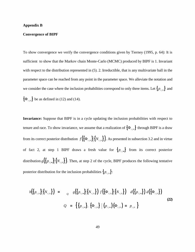
To show convergence we verify the convergence conditions given by Tierney (1995, p. 64): It is

sufficient to show that the Markov chain Monte-Carlo (MCMC) produced by BIPF is 1. Invariant

with respect to the distribution represented in (5). 2. Irreductible, that is any multivariate ball in the

parameter space can be reached from any point in the parameter space. We alleviate the notation and

we consider the case where the inclusion probabilities correspond to only three items. Let kjip and

kjiΦ be as defined in (12) and (14).

Invariance: Suppose that BIPF is in a cycle updating the inclusion probabilities with respect to

tenure and race. To show invariance, we assume that a realization of kjiΦ through BIPF is a draw

from its correct posterior distribution (((( ))))kjikji Nf Φ . As presented in subsection 3.2 and in virtue

of fact 2, at step 1 BIPF draws a fresh value for ++++jip from its correct posterior

distribution (((( ))))kjiji Npg ++++ . Then, at step 2 of the cycle, BIPF produces the following tentative

posterior distribution for the inclusion probabilities kjip :

(((( )))) (((( )))) (((( )))) (((( )))) (((( ))))

(((( )))) (((( )))) kjikjijikjiji

kjijikjikjikjijikjikji

pppQ

dpdNfNpgNph Q

========

====

++++++++

++++++++

ΦΦ

ΦΦ

,

(22)

50

Now we argue that the RHS in (22) is in fact the correct posterior distribution for kjip . Indeed, by

fact 3, ++++jip and kjiΦ are independent, and their joint posterior density factors out, as implied in

the integrand. So each BIPF cycle reconstitutes the correct posterior distribution, and so the MCMC

generated through BIPF is invariant under the distribution in (5).

Irreducibility: We consider the full set onmlkjip . For any ball around Θ∈∈∈∈*onmlkjip , we can

form a chain of events, updating each of the nine set sets in (6) in turn through BIPF, that will reach

the ball with a positive probability in at most nine cycles of BIPF. So the MCMC generated through

BIPF is irreducible.

These results for invariance and irreducibility generalize for any hierarchichal log-linear model, and

BIPF converges in those cases.

51

References

DeGroot, M. H. (1970). Optimal Statistical Decisions, McGraw-Hill

Dempster, A. P., Laird, N. M., Rubin, D. B. (1977). “Maximum Likelihood from Incomplete Data

via the EM Algorithm,” Journal of the Royal Statistical Society, Series B, Vol. 39, 1-22.

Fay, R. E., Town, M. K. (1998). “Variance Estimation for the 1998 Census Dress Rehearsal,”

Proceedings of the Section on Survey Research Methods, American Statistical Association.

Fay, R. E. (1996). “Alternative Paradigms for the Analysis of Imputed Survey Data,” Journal the

American Association, 91, 434.

Gelman, A., Meng, X. L. (1996). “Model Checking and Model Improvement,” Markov Chain

Monte Carlo in Practice, Gilks, Richardson, Spiegelhalter Ed., Chapman and Hall.

Gelman, A., Rubin, D. B. (1991). “Simulating the Posterior Distribution of Loglinear

Contingency Table Models,” Unpublished Technical Report, Harvard University.

Kovar, J. G., Whitridge, P. J. (1995). “Imputation of Business Survey Data,” Business Survey

methods, Cox, Binder, Chinnappa, Christianson, Colledge, Kott Ed., Wiley.

Rao, J. N. K., Shao, J. (1992). “Jackknife Variance Estimation with Survey Data under Hot-Deck

Imputation,” Biometrika, 79, 811-812.

Rubin, D. B. (1978), Multiple Imputations for Nonresponse in Surveys, Wiley.

Schafer, J. L. (1997). Analysis of Incomplete Multivariate Data, Chapman & Hall.

52

Tanner, M. A., Wong, W. H. (1986). “The Calculation of Posterior Distribution by Data

Augmentation,” Journal of the American Statistical Association, 82, 528-540.

Thibaudeau, Y., Williams, T., Krenzke T. (1997). “Multivariate Item Imputation for the 2000

Census Short Form,” Proceedings for the Section on Survey Research Methods, American

Statistical Association.

Thibaudeau, Y. (1988). Approximating the Moments of A Multimodal Posterior Distribution

with the Method of Laplace, Department of Statistics, Carnegie Mellon University, Ph.D.

Dissertation.

Tierney, L. (1996). “Introduction to General State-Space Markov Chain Theory,” Markov

Chain Monte Carlo in Practice, Gilks, Richardson, Spiegelhalter Ed., Chapman and Hall.

Tierney, L., Kadane, J. B. (1986) “Accurate Approximations for Posterior Moments and

Marginal Densities,” Journal of the American Statistical Association, 81, 82-86.

Treat, J. B. (1994). Summary of the 1990 Census Imputation Procedures for the 100 % Population

and Housing Items, DSSD REX Memorandum Series BB-11, US Census Bureau.

Zanutto, E., Zaslavsky, A. M. (1997). “Modeling Census Mailback Questionnaires, Administrative

Records, and Sampled Nonresponse Followup, to Impute Census Nonrespondents,”

Proceedings of the Section on Survey Research Methods, American Statistical Association.

Williams, T. R. (1998). “Imputing Person Age for the 2000 Census short Form: A Model Based

Approach”, Proceedings of the Section on Survey Research Methods, American Statistical

Association.