model predictive control for autonomous and semiautonomous...
TRANSCRIPT

Model Predictive Control for Autonomous and Semiautonomous Vehicles
by
Yiqi Gao
A dissertation submitted in partial satisfaction of the
requirements for the degree of
Doctor of Philosophy
in
Engineering - Mechanical Engineering
in the
Graduate Division
of the
University of California, Berkeley
Committee in charge:
Professor Francesco Borrelli, ChairProfessor J. Karl Hedrick
Professor Laurent El Ghaoui
Spring 2014
Model Predictive Control for Autonomous and Semiautonomous Vehicles
Copyright 2014by
Yiqi Gao
1
Abstract
Model Predictive Control for Autonomous and Semiautonomous Vehicles
by
Yiqi Gao
Doctor of Philosophy in Engineering - Mechanical Engineering
University of California, Berkeley
Professor Francesco Borrelli, Chair
In this thesis we consider the problem of designing and implementing Model Predictive Con-trollers (MPC) for lane keeping and obstacle avoidance of autonomous or semi-autonomousground vehicles. Vehicle nonlinear dynamics, fast sampling time and limited computationalresources of embedded automotive hardware make it a challenging control design problem.MPC is chosen because of its capability of systematically taking into account nonlinearities,future predictions and operating constraints during the control design stage.
We start from comparing two different MPC based control architectures. With a giventrajectory representing the driver intent, the controller has to autonomously avoid obstacleson the road while trying to track the desired trajectory by controlling front steering angleand differential braking. The first approach solves a single nonlinear MPC problem for bothreplanning and following of the obstacle free trajectories. While the second approach uses ahierarchical scheme. At the high-level, new trajectories are computed on-line, in a recedinghorizon fashion, based on a simplified point-mass vehicle model in order to avoid the obstacle.At the low-level an MPC controller computes the vehicle inputs in order to best follow thehigh level trajectory based on a higher fidelity nonlinear vehicle model. Experimental resultsof both approaches on icy roads are shown. The experimental as well as simulation resultsare used to compare the two approaches. We conclude that the hierarchical approach is morepromising for real-time implementation and yields better performance due to its ability ofhaving longer prediction horizon and faster sampling time at the same time.
Based on the hierarchical approach for autonomous drive, we propose a hierarchicalMPC framework for semi-autonomous obstacle avoidance, which decides the necessity ofcontrol intervention based on the aggressiveness of the evasive maneuver necessary to avoidcollisions. The high level path planner plans obstacle avoiding maneuvers using a specialkind of curve, the clothoid. The usage of clothoids have a long history in highway design androbotics control. By optimizing over a small number of parameters, the optimal clothoidssatisfying the safety constraints can be determined. The same parameters also indicatethe aggressiveness of the avoiding maneuver and thus can be used to decide whether acontrol intervention is needed before its too late to avoid the obstacle. In the case of control

2
intervention, the low level MPC with a nonlinear vehicle model will follow the plannedavoiding maneuver by taking over control of the steering and braking. The controller isvalidated by both simulations and experimental tests on an icy track.
In the proposed autonomous hierarchical MPC where the point mass vehicle model isused for high level path replanning, despite of its successful avoidance of the obstacle, thecontroller’s performance can be largely improved. In the test, we observed big deviations ofthe actual vehicle trajectory from the high level planned path. This is because the point massmodel is overly simplified and results in planned paths that are infeasible for the real vehicleto track. To address this problem, we propose an improved hierarchical MPC frameworkbased on a special coordinate transformation in the high level MPC. The high level uses anonlinear bicycle vehicle model and utilizes a coordinate transformation which uses vehicleposition along a path as the independent variable. That produces high level planned pathswith smaller tracking error for the real vehicle while maintaining real-time feasibility. Thelow level still uses an MPC with higher fidelity model to track the planned path. Simulationsshow the method’s ability to safely avoid multiple obstacles while tracking the lane centerline.Experimental tests on an autonomous passenger vehicle driving at high speed on an icy trackshow the effectiveness of the approach.
In the last part, we propose a robust control framework which systematically handles thesystem uncertainties, including the model mismatch, state estimation error, external distur-bances and etc. The framework enforces robust constraint satisfaction under the presenceof the aforementioned uncertainties. The actual system is modeled by a nominal systemwith an additive disturbance term which includes all the uncertainties. A “Tube-MPC”approach is used, where a robust positively invariant set is used to contain all the possibletracking errors of the real system to the planned path (called the “nominal path”). Thusall the possible actual state trajectories in time lie in a tube centered at the nominal path.A nominal NMPC controls the tube center to ensure constraint satisfaction for the wholetube. A force-input nonlinear bicycle vehicle model is developed and used in the RNMPCcontrol design. The robust invariant set of the error system (nominal system vs. real system)is computed based on the developed model, the associated uncertainties and a predefineddisturbance feedback gain. The computed invariant set is used to tighten the constraints inthe nominal NMPC to ensure robust constraint satisfaction. Simulations and experimentson a test vehicle show the effectiveness of the proposed framework.

i
This dissertation is lovingly dedicated to my parents for their eternal and unconditionallove, support and encouragement.
ii
Contents
Contents ii
List of Figures iv
List of Tables viii
1 Introduction 11.1 Motivation and Background . . . . . . . . . . . . . . . . . . . . . . . . . . . 11.2 Thesis Layout . . . . . . . . . . . . . . . . . . . . . . . . . . . . . . . . . . . 4
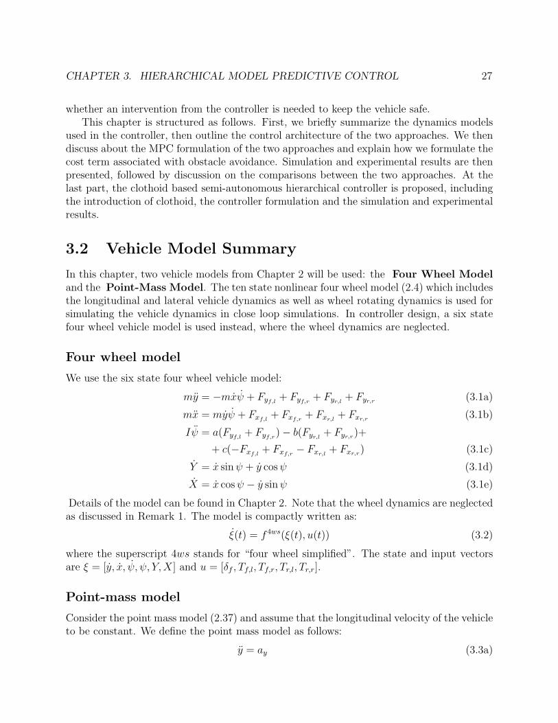
2 Vehicle Models 72.1 Introduction . . . . . . . . . . . . . . . . . . . . . . . . . . . . . . . . . . . . 72.2 Nonlinear Four Wheel Model . . . . . . . . . . . . . . . . . . . . . . . . . . . 102.3 Nonlinear Bicycle Model . . . . . . . . . . . . . . . . . . . . . . . . . . . . . 132.4 Tire Models . . . . . . . . . . . . . . . . . . . . . . . . . . . . . . . . . . . . 162.5 Linear Bicycle Model . . . . . . . . . . . . . . . . . . . . . . . . . . . . . . . 222.6 Point Mass Model . . . . . . . . . . . . . . . . . . . . . . . . . . . . . . . . . 242.7 Concluding Remarks . . . . . . . . . . . . . . . . . . . . . . . . . . . . . . . 24
3 Hierarchical Model Predictive Control 263.1 Introduction . . . . . . . . . . . . . . . . . . . . . . . . . . . . . . . . . . . . 263.2 Vehicle Model Summary . . . . . . . . . . . . . . . . . . . . . . . . . . . . . 273.3 MPC Control Architectures for An Obstacle Avoiding Path Replanner on
Slippery Surface . . . . . . . . . . . . . . . . . . . . . . . . . . . . . . . . . . 283.4 MPC Controller Formulation . . . . . . . . . . . . . . . . . . . . . . . . . . . 303.5 Simulation and Experimental Results . . . . . . . . . . . . . . . . . . . . . . 343.6 Concluding Remarks on Control Architecture Comparison . . . . . . . . . . 413.7 Clothoid Based Semi-Autonomous Hierarchical MPC for Obstacle Avoidance 413.8 Concluding Remarks . . . . . . . . . . . . . . . . . . . . . . . . . . . . . . . 47
4 Spatial Model Predictive Control 494.1 Introduction . . . . . . . . . . . . . . . . . . . . . . . . . . . . . . . . . . . . 494.2 Vehicle model . . . . . . . . . . . . . . . . . . . . . . . . . . . . . . . . . . . 50

iii
4.3 MPC control architecture with obstacle avoidance . . . . . . . . . . . . . . . 524.4 Simulation and experimental results . . . . . . . . . . . . . . . . . . . . . . . 544.5 Concluding Remarks . . . . . . . . . . . . . . . . . . . . . . . . . . . . . . . 58
5 Robust Nonlinear Model Predictive Control 615.1 Introduction . . . . . . . . . . . . . . . . . . . . . . . . . . . . . . . . . . . . 615.2 Invariant set and robust MPC . . . . . . . . . . . . . . . . . . . . . . . . . . 625.3 Modeling . . . . . . . . . . . . . . . . . . . . . . . . . . . . . . . . . . . . . . 665.4 Invariant set computation . . . . . . . . . . . . . . . . . . . . . . . . . . . . 705.5 Safety constraints . . . . . . . . . . . . . . . . . . . . . . . . . . . . . . . . . 735.6 Robust predictive control design . . . . . . . . . . . . . . . . . . . . . . . . . 735.7 Simulation results . . . . . . . . . . . . . . . . . . . . . . . . . . . . . . . . . 745.8 Experimental results . . . . . . . . . . . . . . . . . . . . . . . . . . . . . . . 775.9 Conclusions . . . . . . . . . . . . . . . . . . . . . . . . . . . . . . . . . . . . 88
Bibliography 89
iv
List of Figures
2.1 Vehicle body fixed frame of reference. . . . . . . . . . . . . . . . . . . . . . . . . 82.2 Two commonly used frameworks for modeling of vehicle’s position and orientation. 92.3 Four wheel model notation. . . . . . . . . . . . . . . . . . . . . . . . . . . . . . 102.4 Tire model notations. . . . . . . . . . . . . . . . . . . . . . . . . . . . . . . . . . 122.5 Modelling notation depicting the forces in the vehicle body-fixed frame (Fx⋆ and
Fy⋆), the forces in the tire-fixed frame (Fl⋆ and Fc⋆), and the rotational andtranslational velocities. . . . . . . . . . . . . . . . . . . . . . . . . . . . . . . . . 14
2.6 Lateral and longitudinal tire forces at different values of friction coefficients. . . 172.7 Lateral and longitudinal tire forces in combined cornering and braking/driving,
with µ = 0.9. . . . . . . . . . . . . . . . . . . . . . . . . . . . . . . . . . . . . . 192.8 Lateral and longitudinal tire forces as functions of slip ratio and slip angle in
combined cornering and braking/driving, with µ = 0.9. . . . . . . . . . . . . . . 202.9 Lateral tire forces from the modified Fiala tire model at different levels of brak-
ing/driving. . . . . . . . . . . . . . . . . . . . . . . . . . . . . . . . . . . . . . . 212.10 Linearized lateral tire forces in small slip angle region compared to Pacejka model,
with s = 0 and µ = 0.9. . . . . . . . . . . . . . . . . . . . . . . . . . . . . . . . 22
3.1 Reference state trajectory of the double lane change path to be followed. . . . . 293.2 Two different architectures of controller design. . . . . . . . . . . . . . . . . . . 303.3 Graphical representation of dk,t,j, pxt,j and pyt,j . . . . . . . . . . . . . . . . . . . 323.4 The test vehicle. . . . . . . . . . . . . . . . . . . . . . . . . . . . . . . . . . . . 363.5 Experimental result: Test results of the one-level MPC at vehicle speed 40 Kph.
The red box represents the obstacle. . . . . . . . . . . . . . . . . . . . . . . . . 363.6 Experimental result: Test results of the two-level MPC at vehicle speed 45 Kph.
The red bos represents the obstacle. . . . . . . . . . . . . . . . . . . . . . . . . . 363.7 Experimental result: Test results of the two-level MPC at vehicle speed 55 Kph.
The red box represents the obstacle. . . . . . . . . . . . . . . . . . . . . . . . . 373.8 Experimental result: Replanned paths from the high-level path replanner in two-
level MPC. Vehicle speed is 55 Kph. . . . . . . . . . . . . . . . . . . . . . . . . 373.9 Experimental result: Replanned paths from high-level when the communication
from high-level to low-level is cut off. Vehicle speed is 55 Kph. . . . . . . . . . . 38
v
3.10 Simulation results: At speed of 70Kph, the one-level MPC becomes unstable evenif given enough computation time. While the two-level MPC is able to stabilizethe vehicle in the same situation. . . . . . . . . . . . . . . . . . . . . . . . . . . 40
3.11 Lane change paths with different aggressiveness. Each is generated by connectingfour pieces of clothoids. The upper figure shows the shapes of the paths in globalframe. The lower figure shows the piecewise affine relation between curvatureand curve length for each path. . . . . . . . . . . . . . . . . . . . . . . . . . . . 42
3.12 Ad-hoc Clothoid parameters setup for obstacle constraints. . . . . . . . . . . . . 443.13 Simulation result: Various lane change maneuvers are compared. As the vehicle
approaches the obstacle the planned paths become more aggressive (high curva-tures). . . . . . . . . . . . . . . . . . . . . . . . . . . . . . . . . . . . . . . . . . 45
3.14 Simulation result: In the upper plot an attentive driver is assumed. The low-levelcontrol takes over when the planned path becomes aggressive. In the lower plotthe low-level control takes over for a distracted driver and the result is a smootherand safer path. . . . . . . . . . . . . . . . . . . . . . . . . . . . . . . . . . . . . 46
3.15 Experimental results: Vehicle successfully avoids the obstacle using maneuversbased on clothoids. . . . . . . . . . . . . . . . . . . . . . . . . . . . . . . . . . . 46
3.16 Experimental result: Actual path of the vehicle deviates from the planned pathdue to model mismatch and caused infeasibility of tracking. Braking was invokedto enlarge the feasible region in that situation. . . . . . . . . . . . . . . . . . . . 47
4.1 The curvilinear coordinate system. The dynamics are derived about a curvedefining the center-line of a track. The coordinate s defines the arc-length alongthe track. The relative spatial coordinates ey and eψ are shown. . . . . . . . . . 51
4.2 Architecture of the two-level MPC. A spatial vehicle model is used for high-levelpath planning. A four-wheel vehicle model is used for low-level path tracking. . 52
4.3 Simulated result: The vehicle entered the maneuver at 50 kph. The green linesare planned paths from the high-level which are updated every 200 ms. The blackline is the actual trajectory the vehicle traveled. . . . . . . . . . . . . . . . . . . 56
4.4 Experimental result: The vehicle entered the maneuver at 50 kph. Friction co-efficient of the ground was approximately 0.3. The vehicle avoided the obstacleand continued to track the lane center. The green lines are planned paths fromthe high-level which were updated every 200 ms. The black line is the actualtrajectory the vehicle traveled. . . . . . . . . . . . . . . . . . . . . . . . . . . . . 57
4.5 Experimental result: The vehicle entered the maneuver at 50 kph. Friction coeffi-cient of the ground was approximately 0.3. The vehicle avoided the two obstaclesand continued to track the lane center. . . . . . . . . . . . . . . . . . . . . . . . 57
4.6 Experimental result: The vehicle entered the maneuver at 50 kph. Friction coeffi-cient of the ground was approximately 0.3. The vehicle avoided the first obstacleand continued to track the lane center until the second obstacle came into sight.It then turned left to avoid the second obstacle. . . . . . . . . . . . . . . . . . . 58

vi
4.7 Simulation result comparison with the controller proposed in [23]. In both casesthe high levels replan every 200ms. The same low level path follower is used,which uses a nonlinear four wheel model and runs every 50ms. . . . . . . . . . . 59
5.1 Modeling notation depicting the forces in the vehicle body-fixed frame (Fx⋆ andFy⋆), the forces in the tire-fixed frame (Fl⋆ and Fc⋆), and the rotational andtranslational velocities. The relative coordinates ey and eψ are illustrated on thesketch of the road as well as the road tangent ψd. . . . . . . . . . . . . . . . . . 66
5.2 Illustration of center of percussion. p denotes the distance from CoG to CoP . . 685.3 Lateral tire force. µ is 0.5 in Pacejka tire model. When βr varies moderately, Fc
behaves similar within the linear region. . . . . . . . . . . . . . . . . . . . . . . 695.4 One-step model prediction error (equation (5.31)) of 47 testing trials. . . . . . . 725.5 Simulation result: The vehicle enters the maneuver at 50Kph. The dashed black
line and blue line are the nominal and actual vehicle trajectories respectively. Thegreen dot-dashed lines indicate the robust bounds around the nominal trajectory.The actual vehicle path is seen to be very close to the nominal one and withinthe robust bounds. . . . . . . . . . . . . . . . . . . . . . . . . . . . . . . . . . . 75
5.6 Simulation result: Control inputs during the simulation in figure 5.5. βf is thebraking/throttle ratio for the front wheels and βr for the rear wheels. We enableboth braking and throttle on the wheels in simulation. . . . . . . . . . . . . . . 76
5.7 Simulation result: Trajectories of nominal MPC controlled system under a ran-dom external disturbance. . . . . . . . . . . . . . . . . . . . . . . . . . . . . . . 77
5.8 Simulation result: Trajectories of RNMPC controlled system under a randomexternal disturbance. . . . . . . . . . . . . . . . . . . . . . . . . . . . . . . . . . 77
5.9 Simulation result: Trajectories of RNMPC controlled system under unknown andconstantly changing tire road friction coefficients. . . . . . . . . . . . . . . . . . 78
5.10 The test vehicle. . . . . . . . . . . . . . . . . . . . . . . . . . . . . . . . . . . . 795.11 Experimental result: The vehicle enters the maneuver at 50Kph. The dashed
black line and blue line are the nominal and actual vehicle trajectories respec-tively. The green dot-dashed lines indicate the robust bounds around the nominaltrajectory. The actual vehicle path is seen to be very close to the nominal oneand within the robust bounds. µ ≃ 0.3. . . . . . . . . . . . . . . . . . . . . . . . 80
5.12 Experimental result: A plot of 4 states of the vehicle, [y, ψ, eψ, ey], during theexperiment of Figure 5.11. The nominal and actual states are shown in dashedblack and solid blue lines respectively. The red dot-dashed lines indicate therobust bounds on each state. . . . . . . . . . . . . . . . . . . . . . . . . . . . . . 80
5.13 Experimental result: The steering and braking input to the vehicle during theexperiment of Figure 5.11. The braking is applied by the controller at the begin-ning of the maneuver to reduce the speed so that the avoiding maneuver can bemore smooth. . . . . . . . . . . . . . . . . . . . . . . . . . . . . . . . . . . . . . 81
vii
5.14 Experimental result: The vehicle enters the maneuver at 80Kph. The dashedblack line and blue line are the nominal and actual vehicle trajectories respec-tively. The green dot-dashed lines indicate the robust bounds around the nominaltrajectory. The actual vehicle path is seen to be very close to the nominal oneand within the robust bounds. µ ≃ 0.3. . . . . . . . . . . . . . . . . . . . . . . . 81
5.15 Experimental result: A plot of 4 states of the vehicle, [y, ψ, eψ, ey], during theexperiment of Figure 5.14. The nominal and actual states are shown in dashedblack and solid blue lines respectively. The red dot-dashed lines indicate therobust bounds on each state. . . . . . . . . . . . . . . . . . . . . . . . . . . . . . 82
5.16 Experimental result: The steering and braking input to the vehicle during theexperiment of Figure 5.14. . . . . . . . . . . . . . . . . . . . . . . . . . . . . . . 82
5.17 Experimental result: Avoiding a moving obstacle. Vehicle speed is 50 Kph, ob-stacle moves at 18 Kph. The obstacle position at time t0, t1 and t3 during thetest are shown in dash red. The vehicle position at the corresponding times aremarked with blue circles. µ ≃ 0.3. . . . . . . . . . . . . . . . . . . . . . . . . . . 83
5.18 Experimental result: A plot of 4 states of the vehicle, [y, ψ, eψ, ey], during theexperiment of Figure 5.19. The nominal and actual states are shown in dashedblack and solid blue lines respectively. The red dot-dashed lines indicate therobust bounds on each state. . . . . . . . . . . . . . . . . . . . . . . . . . . . . . 84
5.19 Experimental result: The steering and braking input to the vehicle during theexperiment of Figure 5.19. . . . . . . . . . . . . . . . . . . . . . . . . . . . . . . 84
5.20 Experimental result: Vehicle trajectory. The vehicle enters the maneuver at50Kph. µ ≃ 0.3. . . . . . . . . . . . . . . . . . . . . . . . . . . . . . . . . . . . . 85
5.21 Experimental resultA plot of 4 states of the vehicle, [y, ψ, eψ, ey], during the ex-periment of Figure 5.20. The nominal and actual states are shown in dashedblack and solid blue lines respectively. The red dot-dashed lines indicate therobust bounds on each state. . . . . . . . . . . . . . . . . . . . . . . . . . . . . . 85
5.22 Experimental result: The steering and braking input to the vehicle during theexperiment of Figure 5.20. . . . . . . . . . . . . . . . . . . . . . . . . . . . . . . 86
5.23 Experimental result: Vehicle trajectory on an ice track. The vehicle enters themaneuver at 35Kph. The actual µ on the track is 0.1, while the controller is setup for µ = 0.3 on snow track. . . . . . . . . . . . . . . . . . . . . . . . . . . . . 86
5.24 Experimental result: A plot of 4 states of the vehicle, [y, ψ, eψ, ey], during theexperiment of Figure 5.23. The nominal and actual states are shown in dashedblack and solid blue lines respectively. The red dot-dashed lines indicate therobust bounds on each state. . . . . . . . . . . . . . . . . . . . . . . . . . . . . . 87
5.25 Experimental result: The steering and braking input to the vehicle during theexperiment of Figure 5.23. . . . . . . . . . . . . . . . . . . . . . . . . . . . . . . 87

viii
List of Tables
1.1 U.S.A. Traffic Fatality Data Report . . . . . . . . . . . . . . . . . . . . . . . . 1
3.1 Comutation Time of One-level and Two-level MPC at Vehicle Speed of 40 Kph. 39
5.1 Simulation Parameters . . . . . . . . . . . . . . . . . . . . . . . . . . . . . . . . 755.2 Real-Time Design Parameters for Experimental Test . . . . . . . . . . . . . . . 78
ix
Acknowledgments
My greatest thanks go to Prof. Francesco Borrelli, my adviser and mentor. Without hishelp and guidance, I wouldn’t have accomplished this work. More importantly, his passion,meticulosity, diligence and wisdom always inspire and inspirit me. These influences are thegreater gifts for me to take into my life and work.
I want to express my most sincere thanks to Eric Tseng for his valuable suggestions in myresearch and tremendous help in the testing. I want to thank all the Professors from insideand outside the Mechanical Engineering Department who shared their knowledge and expe-rience with me, especially, Prof. Karl Hedrick. A lot of thanks also go to Mitch McConnelland Vladimir Ivanovic from Ford Motor company for their valuable help in conducting thetests.
My special thanks go to my colleagues and friends Theresa Lin, Andrew Gray and AshwinCarvalho for their accompany through the hardest and happiest time. I also want to thankMiroslav Baric and Yudong Ma for their sharing as seniors through the starting years of myPh.D. life. Thanks to all the friends in or used to be in MPC lab, the birthday cake is sweet!
I thank all the friends that walked into my everyday life for sharing the happiness andsadness and bringing the feeling of home when far from it.
1
Chapter 1
Introduction
1.1 Motivation and Background
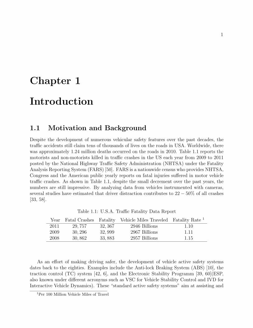
Despite the development of numerous vehicular safety features over the past decades, thetraffic accidents still claim tens of thousands of lives on the roads in USA. Worldwide, therewas approximately 1.24 million deaths occurred on the roads in 2010. Table 1.1 reports themotorists and non-motorists killed in traffic crashes in the US each year from 2009 to 2011posted by the National Highway Traffic Safety Administration (NHTSA) under the FatalityAnalysis Reporting System (FARS) [50]. FARS is a nationwide census who provides NHTSA,Congress and the American public yearly reports on fatal injuries suffered in motor vehicletraffic crashes. As shown in Table 1.1, despite the small decrement over the past years, thenumbers are still impressive. By analyzing data from vehicles instrumented with cameras,several studies have estimated that driver distraction contributes to 22− 50% of all crashes[33, 58].
Table 1.1: U.S.A. Traffic Fatality Data Report
Year Fatal Crashes Fatality Vehicle Miles Traveled Fatality Rate 1
2011 29, 757 32, 367 2946 Billions 1.102009 30, 296 32, 999 2967 Billions 1.112008 30, 862 33, 883 2957 Billions 1.15
As an effort of making driving safer, the development of vehicle active safety systemsdates back to the eighties. Examples include the Anti-lock Braking System (ABS) [10], thetraction control (TC) system [42, 6], and the Electronic Stability Programm [39, 60](ESP,also known under different acronyms such as VSC for Vehicle Stability Control and IVD forInteractive Vehicle Dynamics). These “standard active safety systems” aim at assisting and
1Per 100 Million Vehicle Miles of Travel

CHAPTER 1. INTRODUCTION 2
improving the driver’s control over the vehicle by avoiding undesired situations, such as wheellocking in braking (ABS), tire slipping (TC), and lose of steering control (ESP). While thesesystems’ effectiveness in general has been widely acknowledged, they can offer little helpwhen the driver is inattentive, which unfortunately contributes to 22 − 50% of all crashesaccording to some studies[33, 58]. More recent developments in “advanced active safetysystems” introduce additional sensors such as onboard cameras, radars, infrared sensorsetc., and additional actuators such as active steering or active suspensions. Vehicles equippedwith these systems are able to identify obstacles on the road such as pedestrians as well asthe lane markers. They can perform emergency maneuvers (mostly emergency braking) toavoid collisions or apply assist steering to avoid lane departures. An example of vehicle withadvanced active safety systems is the Volvo S60 equipped with cameras and radars in order toimplement a fully autonomous braking [11, 40]. An even more ambitious approach towardsdriving safety is the development of autonomous driving systems. These systems aim atdriving the vehicle fully autonomously by controlling the steering, braking and throttling,examples include the Darpa Grant Challenge Car [3, 48] and the Google Car [29, 38].
This thesis focuses on Model Predictive Control (MPC) of autonomous and semiau-tonomous vehicles. MPC is the only control technology that can systematically take intoaccount the future predictions and system operating constraints in design stage [46, 49]. Thatmakes it a suitable choice for autonomous drive where the system faces dynamically changingenvironment and has to satisfy crucial safety constraints (such as obstacle avoidance) as wellas actuator constraints.
In MPC, a model of the plant is used to predict the future evolution of the system. Basedon this prediction, at each time step t, a performance index is optimized under operatingconstraints with respect to a sequence of future input moves. The first of such optimal movesis the control action applied to the plant at time t. At time t +1, a new optimization issolved over a shifted prediction horizon. In general, the following finite horizon optimizationproblem is solved at each time step t:
minUt
JN(ξt, Ut) =
t+Hp,hl−1∑k=t
Cost(ξk,t, uk,t) (1.1a)
subj. to ξk+1,t = f(ξk,t, uk,t) k = t, ..., t+N − 1, (1.1b)
ξk,t ∈ Ξt k = t, ..., t+N, (1.1c)
uk,t ∈ U k = t, ..., t+N − 1, (1.1d)
ξt,t = ξ(t), (1.1e)
where the symbol vk,t stands for “ the variable v at time k predicted at time t”, N is theprediction horizon. ξ is the state of the system and in this thesis includes the lateral andlongitudinal vehicle velocities, yaw and yaw rate, and vehicle position. u is the control inputto the system and in this thesis includes the steering angle, braking torque and throttle.The function f(ξ, u) in (1.1b) allows to predict the future system states based on the current

CHAPTER 1. INTRODUCTION 3
states and control inputs. (1.1c) and (1.1d) are the state and input constraints the controllerhas to respect. The cost in (1.1a) can be any performance index and in this thesis can includepenalties on state tracking error, penalties on inputs, penalties on input change rate and etc.
The earliest implementations of MPC were on “slow” plants such as those in processindustry [52, 12, 5], where the plant dynamics are sufficiently “slow” for the on-line com-putation needed in implementation. Parallel advances in theory and computing systemshave enlarged the range of applications where real-time MPC can be applied [7, 8, 31, 22,64, 13]. Yet, for a wide class of fast applications, the computational burden of NonlinearMPC (NMPC) is still a barrier. As an example, in [9] an NMPC has been implementedon a passenger vehicle for path following via an Active Front Steering (AFS) system at 20Hz, by using the state of the art optimization solvers and rapid prototyping systems. It isshown that the real-time execution is limited to low vehicle speeds on icy roads, because ofits computational complexity.
This thesis focuses on developing nonlinear model predictive controllers for autonomousand semiautonomous driving, particularly for obstacle avoidance and lane keeping. It willshow that by proper modeling and formulation, the autonomous and semiautonomous drivingcan be achieved with NMPC on standard rapid prototyping platform with limited compu-tational resource. In particular, the main contributions of this thesis include:
1. The design of a hierarchical MPC scheme for autonomous obstacle avoidance and lanekeeping. The autonomous driving problem is decomposed into two levels, a high levelpath planner/replanner which uses an MPC with point mass vehicle model to planobstacle free paths with long prediction horizons, and a low level path follower whichuses an MPC with a higher fidelity vehicle model to follow the planned path withshort prediction horizons. The decomposition of the problem reduces the computa-tional complexity compared to a single level MPC approach and results in improvedperformance in real-time implementation.
2. The design of a hierarchical MPC scheme for a semi-autonomous active safety systemthat is able to determine the time of intervention and avoid upcoming collisions withobstacles. The high level MPC uses a special kind of curve, the clothoid, to plan obsta-cle avoiding maneuvers. The use of clothoid makes it possible to plane feasible vehicletrajectories with few parameters and thus with low computational burden. The pa-rameters also give a measure to the necessary aggressiveness of the avoiding maneuverand thus can be used to determine whether a control intervention is necessary. In thecase of intervention, the low level MPC with a higher fidelity vehicle model will followthe high level planned path by controlling the steering and braking.
3. The design of a spatial predictive controller for autonomous obstacle avoidance and lanekeeping. It is an improved approach over the point mass model hierarchical MPC. Thehierarchical scheme as well as the low level path follower are kept the same. The highlevel uses a nonlinear bicycle vehicle model and utilizes a coordinate transformationwhich uses vehicle position along a path as the independent variable. That results in
CHAPTER 1. INTRODUCTION 4
high level planned paths that are more trackable for the real vehicle while maintainingreal-time feasibility and thus improves the performance of overall system.
4. The design of a robust nonlinear predictive control framework based on the “Tube-MPC” approach. The framework presents a systematic way of enforcing robust robustconstraint satisfaction under the presence of model mismatch and disturbances duringthe MPC design stage. A force-input nonlinear bicycle vehicle model is developedand used in the RNMPC control design. A robust invariant set is used to tighten theconstraints in order to guarantee that state and input constraints are satisfied in thepresence of disturbances and model error.
1.2 Thesis Layout
The remainder of this thesis is structured as follows:
• Chapter 2 describes the vehicle models used in control design and simulations forautonomous and semiautonomous vehicles. The tire ground reaction forces are theonly external forces acting on the vehicle, if exclude the gravity force and the muchless significant aerodynamic forces. Unfortunately, the tire forces are highly nonlinearin part of the operational region and the lateral and longitudinal tire dynamics arehighly coupled in the same region. That is the most important source of the nonlinearbehavior of vehicle dynamics and coupling of lateral and longitudinal vehicle dynamics.Simplifications can be made at a cost of greater model mismatch and restrictions onoperation range. The proper choice over various models is an important aspect in theMPC design.
Three tire models are introduced: 1, the Pacejka model, a complex nonlinear semi-empirical tire model being able to describe the nonlinear and coupling behavior of tireforces under wide operation range; 2, the modified Fiala model, a simplified nonlineartire model which also captures the nonlinear and coupling behavior; 3, the linear tiremodel only for pure cornering or pure braking/throttling.
Using rigid body dynamics and the tire models, four vehicle models with various fideli-ties and complexities are introduced: 1, the nonlinear four wheel vehicle model whichcaptures both lateral and longitudinal vehicle dynamics and models the tire forces fromeach of the four tires using the Pacejka model; 2, the nonlinear bicycle model whichis simplified from the nonlinear four wheel model by lumping the left and right tirestogether at the front and rear wheel axels; 3, the linear bicycle model which is furthersimplified from the nonlinear bicycle model by assuming constant longitudinal velocityand the use of linear tire model for pure cornering; 4, the simplest point mass model,where the vehicle is treated as a point with a given mass and no tire model is usedexpect a constraint that the tire forces being inside the friction circle.
CHAPTER 1. INTRODUCTION 5
• Chapter 3 compares two approaches to the autonomous obstacle avoidance problem,the one-level MPC approach and the hierarchical two-level MPC approach. In thefirst approach, the problem is formulated in a single nonlinear MPC problem. In thesecond approach, the controller design is decomposed into two levels. The high-levelNMPC uses a simplified point-mass vehicle model to replan the obstacle free pathwith long prediction horizon. The planed trajectory is fed to the low-level NMPCwhich uses the higher fidelity nonlinear four wheel model to follow the planed pathswith shorter prediction horizon. Simulation and experimental results on an icy-snowhandling track is used to compare the performance and computation time of bothapproaches. Concludes are made that the hierarchical MPC is more promising forreal-time implementation and has better performance due to its lower computationalcomplexity.
Chapter 3 also proposes a hierarchical approach for semi-autonomous obstacle avoid-ance. Where the high level path planner utilizes a special kind of curve, the clothoid,to plan the smoothest path avoiding the obstacle. Very few parameters is needed todetermine the planned path, which is obstacle free and feasible for the vehicle to track.That results in low computational complexity for the high level path planner. Theparameters also gives a measure of the aggressiveness of the avoiding maneuver, pro-viding a suitable indication of whether an intervention from the controller is needed tokeep the vehicle safe. When intervention is decided, the low level NMPC path followertakes control of the steering and braking to follow the planned avoiding maneuver.
• Chapter 4 proposes a spatial predictive control framework for autonomous obstacleavoidance and lane keeping. It is an improved approach over the point mass modelhierarchical MPC. The hierarchical scheme as well as the low level path follower arekept the same. The high level uses a nonlinear bicycle vehicle model and utilizes acoordinate transformation which uses vehicle position along a path as the independentvariable. That results in high level planned paths that are more trackable for the realvehicle while maintaining real-time feasibility and thus improves the performance ofoverall system. The proposed frameworks is validated by experiments on the sameicy-snow handling track.
• Chapter 5 proposes a robust nonlinear predictive control framework based on the“Tube-MPC” approach. The framework presents a systematic way of enforcing robustrobust constraint satisfaction under the presence of model mismatch and disturbancesduring the MPC design stage. The basic idea is to use a control law of the formu = u + K(ξ − ξ) where u and ξ are the nominal control input and system statestrajectories determined by a nominal NMPC. For a given linear controller K, a ro-bust invariant set is computed for the error system. The invariant is used to boundthe maximum deviation of the actual states from the nominal states under the linearcontrol action K. The nominal MPC optimises u and ξ with tightened state and in-put constraints. The tightening is computed as a function of the bounds derived from
CHAPTER 1. INTRODUCTION 6
the robust invariant set. A force-input nonlinear bicycle vehicle model is developedand used in the RNMPC control design. The proposed robust NMPC framework isvalidated by both simulation and experiments.

7
Chapter 2
Vehicle Models
2.1 Introduction
In this chapter, we present several dynamic vehicle models used for control design andsimulation in this thesis. The modeling of vehicle dynamics has been extensively studiedin the past decades. A wide spectrum of vehicle models has appeared in the rich literature[53] [32]. We present a set of models which is suitable for the proposed model based controldesigns.
Figure 2.1 shows a sketch of vehicle body fixed frame of reference and the forces actingon vehicle’s Center of Gravity (CoG). x, y and z are the vehicle’s longitudinal, lateral andvertical axes, respectively. x, y and ψ are the longitudinal, lateral velocities and yaw rate.Fx, Fy andMz are the longitudinal, lateral forces acting on the vehicle CoG and the rotatingmoment about z axes.
The rigid body dynamic equations are:
mx = myψ + Fx, (2.1a)
my = −mxψ + Fy, (2.1b)
Izψ =Mz, (2.1c)
where m is the vehicle mass and I is the vehicle’s moment of inertia about z axis.We use different choices of modeling vehicle’s position and orientation in inertial frames.
Figure 2.2 shows two commonly used setups for modeling the vehicle’s planner motion ininertial frames.
Setup one (Figure 2.2(a)) uses a cartesian coordinate system (X-Y coordinate) for theinertial frame of reference. In Figure 2.2(a), x and y axes are the body fixed coordinatesystem same as in Figure 2.1. The angle ψ is the vehicle’s heading angle, or yaw angle, inthe inertial frame X − Y . ψ is defined positive counterclockwise with ψ = 0 when x axisis aligned with X axis. The vehicle’s 2-D motion in X − Y coordinate can be modeled asfollows:

CHAPTER 2. VEHICLE MODELS 8
x
CoG
z
yϕ&
zM
yF
xF
G
y&
x&
Figure 2.1: Vehicle body fixed frame of reference.
X = x cosψ − y sinψ, (2.2a)
Y = x sinψ + y cosψ. (2.2b)
Setup two (Figure 2.2(b)) uses a curve linear coordinate system s − ey to present thevehicle’s position with respect to a given curve, usually a lane the vehicle is following. Thissetup is particularly useful in environments such as highways and city streets [53]. As shownin Figure 2.2(b), ey is the vehicle’s lateral deviation from the lane center and s is the vehicle’slongitudinal position along the lane center. The angle eψ is the vehicle’s heading angle withrespect to the lane direction. eψ is defined positive counterclockwise with eψ = 0 when xaxis is aligned with the tangent of lane center. The vehicle’s 2-D motion in this setup ismodeled as follows:
eψ = ψ − ψd, (2.3a)
s =1
1− κey· (xcos(eψ)− ysin(eψ)), (2.3b)
ey = x sin(eψ) + y cos(eψ), (2.3c)
where ψ is the vehicle’s yaw rate. ψd is the angle of the tangent to the lane centerline in afixed coordinate frame. κ is the curvature of the lane and is defined positive counterclockwise.
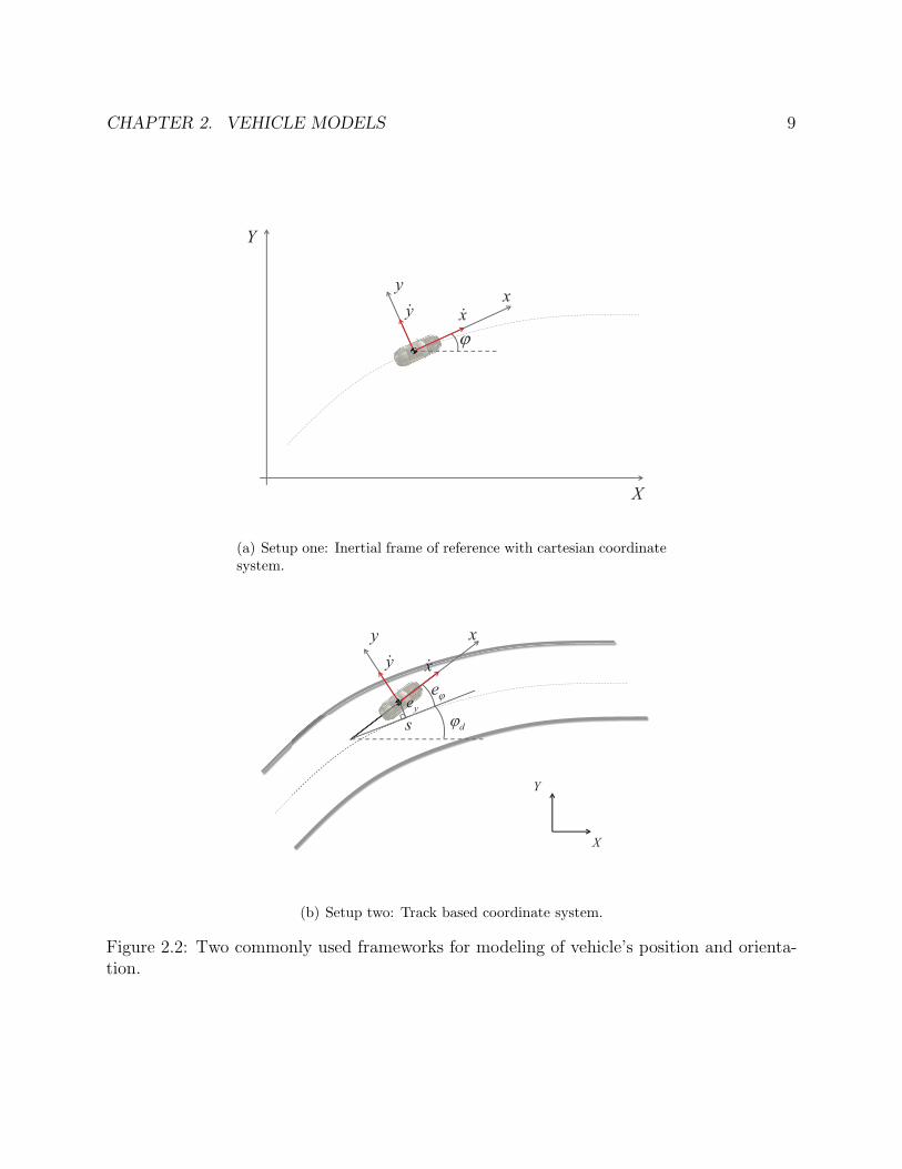
CHAPTER 2. VEHICLE MODELS 9
xy
ϕ
y& x&
X
Y
(a) Setup one: Inertial frame of reference with cartesian coordinatesystem.
ϕe
xy
y& x&
ye
s
Y
X
dϕ
(b) Setup two: Track based coordinate system.
Figure 2.2: Two commonly used frameworks for modeling of vehicle’s position and orienta-tion.
CHAPTER 2. VEHICLE MODELS 10
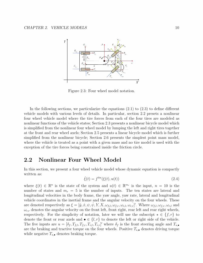
Figure 2.3: Four wheel model notation.
In the following sections, we particularize the equations (2.1) to (2.3) to define differentvehicle models with various levels of details. In particular, section 2.2 presets a nonlinearfour wheel vehicle model where the tire forces from each of the four tires are modeled asnonlinear functions of the vehicle states; Section 2.3 presents a nonlinear bicycle model whichis simplified from the nonlinear four wheel model by lumping the left and right tires togetherat the front and rear wheel axels; Section 2.5 presents a linear bicycle model which is furthersimplified from the nonlinear bicycle; Section 2.6 presents the simplest point mass model,where the vehicle is treated as a point with a given mass and no tire model is used with theexception of the tire forces being constrained inside the friction circle.
2.2 Nonlinear Four Wheel Model
In this section, we present a four wheel vehicle model whose dynamic equation is compactlywritten as:
ξ(t) = f 4w(ξ(t), u(t)) (2.4)
where ξ(t) ∈ Rn is the state of the system and u(t) ∈ Rmr is the input, n = 10 is thenumber of states and mr = 5 is the number of inputs. The ten states are lateral andlongitudinal velocities in the body frame, the yaw angle, yaw rate, lateral and longitudinalvehicle coordinates in the inertial frame and the angular velocity on the four wheels. Theseare denoted respectively as ξ = [y, x, ψ, ψ, Y,X, ωf,l, ωf,r, ωr,l, ωr,r]
′. Where ωf,l, ωf,r, ωr,l andωr,r denotes the angular velocity on the front left, front right, rear left and rear right wheels,respectively. For the simplicity of notation, later we will use the subscript ⋆ ∈ f, r todenote the front or rear axels and • ∈ l, r to denote the left or right side of the vehicle.The five inputs are u = [δf , Tf,l, Tf,r, Tr,l, Tr,r]
′ where δf is the front steering angle and T⋆,•are the braking and tractive torque on the four wheels. Positive T⋆,• denotes driving torquewhile negative T⋆,• denotes braking torque.
CHAPTER 2. VEHICLE MODELS 11
Figure 2.3 defines the notations of the four wheel model. In particular, Fc⋆,• and Fl⋆,•are the lateral (cornering) and longitudinal tire forces in tire frame. Fy⋆,• and Fx⋆,• are thecomponents of the tire forces along the lateral and longitudinal vehicle axes. α⋆,• are thewheel slip angles which are defined later in this section. δf is the front wheel steering angle.a and b are the distances from the CoG to the front and rear axles and c is the distance fromthe CoG to the left/right side at the wheels.
The dynamics in (2.4) can be derived by using the equations of motion about the vehiclesCenter of Gravity (CoG) and coordinate transformations between the inertial frame and thevehicle body frame:
my = −mxψ + Fyf,l + Fyf,r + Fyr,l + Fyr,r , (2.5a)
mx = myψ + Fxf,l + Fxf,r + Fxr,l + Fxr,r , (2.5b)
Iψ = a(Fyf,l + Fyf,r)− b(Fyr,l + Fyr,r)+
+ c(−Fxf,l + Fxf,r − Fxr,l + Fxr,r), (2.5c)
Y = x sinψ + y cosψ, (2.5d)
X = x cosψ − y sinψ, (2.5e)
Iwωf,l = −Flf,lrw + Tf,l − bwωf,l, (2.5f)
Iwωf,r = −Flf,rrw + Tf,r − bwωf,r, (2.5g)
Iwωr,l = −Flr,lrw + Tr,l − bwωr,l, (2.5h)
Iwωr,r = −Flr,rrw + Tr,r − bwωr,r, (2.5i)
where the constant m is the vehicle’s mass. I is the vehicle’s rotational inertia about the zaxis. Iw includes the wheel and driveline rotational inertias. rw is the radius of the wheel.bw is the damping coefficient.
The x and y components of tire forces, Fx⋆,• and Fy⋆,• , are computed as follows:
Fy⋆,• = Fl⋆,• sin δ⋆ + Fc⋆,• cos δ⋆, (2.6a)
Fx⋆,• = Fl⋆,• cos δ⋆ − Fc⋆,• sin δ⋆. (2.6b)
Assumption 1 Only the steering angle at the front wheels can be controlled. Moreover, thefront left and front right wheel steering angles are assumed to be the same. i.e., δf,l = δf,r = δfand δr,• = 0.
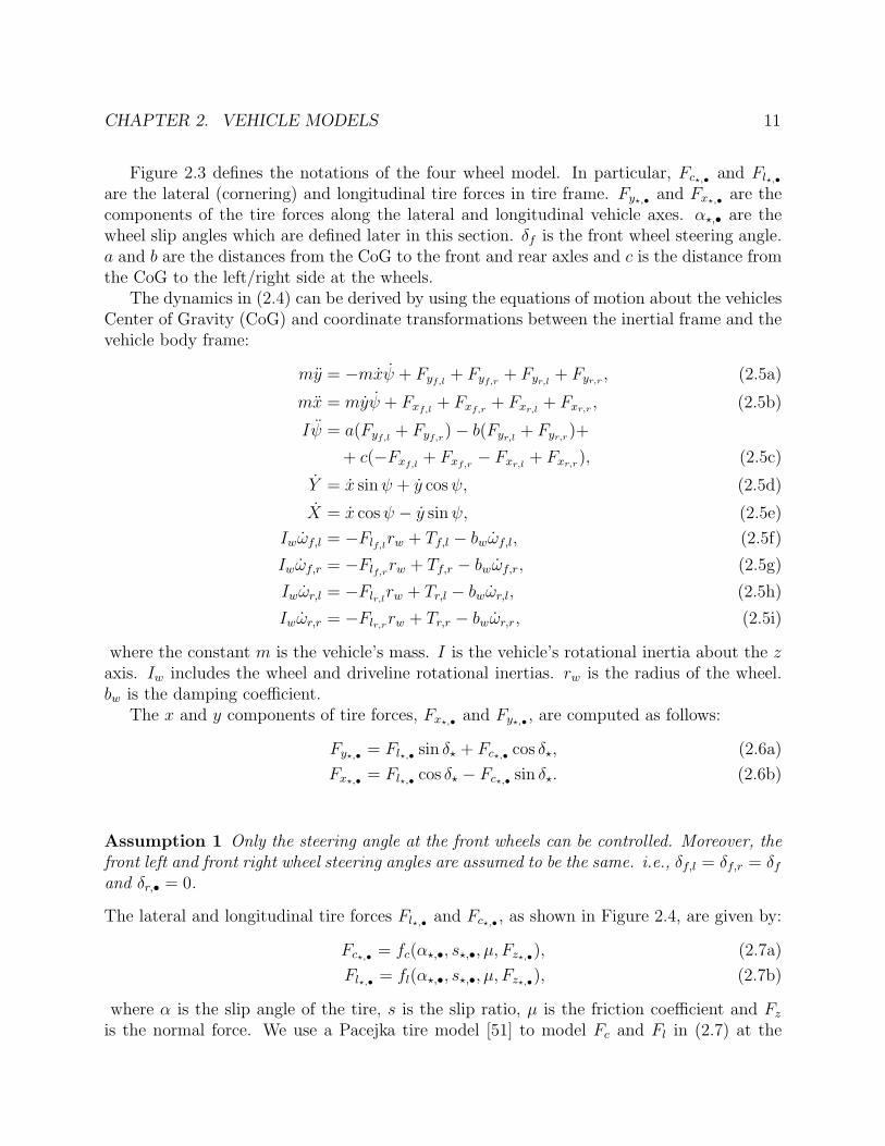
The lateral and longitudinal tire forces Fl⋆,• and Fc⋆,• , as shown in Figure 2.4, are given by:
Fc⋆,• = fc(α⋆,•, s⋆,•, µ, Fz⋆,•), (2.7a)
Fl⋆,• = fl(α⋆,•, s⋆,•, µ, Fz⋆,•), (2.7b)
where α is the slip angle of the tire, s is the slip ratio, µ is the friction coefficient and Fzis the normal force. We use a Pacejka tire model [51] to model Fc and Fl in (2.7) at the
CHAPTER 2. VEHICLE MODELS 12
Figure 2.4: Tire model notations.
four tires. This complex, semi-empirical model is able to describe the tire behavior over thelinear and nonlinear operating ranges of slip ratio, tire slip angle and friction coefficient.
As shown in Figure 2.4, the tire slip angle α⋆,• in (2.7) denotes the angle between thetire velocity and its longitudinal direction. It can be expressed as:
α⋆,• = arctanvc⋆,•vl⋆,•
, (2.8)
where vc⋆,• and vl⋆,• are the lateral and longitudinal wheel velocities computed from:
vc⋆,• = vy⋆,• cos δ⋆ − vx⋆,• sin δ⋆, (2.9a)
vl⋆,• = vy⋆,• sin δ⋆ + vx⋆,• cos δ⋆, (2.9b)
vyf,• = y + aψ vx⋆,l = x− cψ, (2.9c)
vyr,• = y − bψ vx⋆,r = x+ cψ. (2.9d)
The slip ratio is defined as:
s⋆,• =
rω⋆,•
vl⋆,•− 1 if vl⋆,• > rω⋆,•, v = 0 for braking,
1−vl⋆,•rω⋆,•
if vl⋆,• < rω⋆,•, ω = 0 for driving.
(2.10)
The friction coefficient µ is assumed to be a known constant and is the same at all fourwheels.
CHAPTER 2. VEHICLE MODELS 13
We use the static weight distribution to estimate the normal force on the wheel, Fz⋆,• inEquation (2.7). They are approximated as:
Fzf,• =bmg
2(a+ b), Fzr,• =
amg
2(a+ b), (2.11)
where g is the gravitational acceleration.
Remark 1 For control purposes, the wheel dynamics (2.5f)-(2.5i) can be neglected. In thiscase the wheel speed can be assumed to be measured at each sampling time and is kept constantuntil the next available update.
Remark 2 The model (2.5) uses reference framework one (2.2) for position representation.Note one can use the reference framework two (2.3) without affecting the dynamics. i.e.(2.5d)-(2.5e) in (2.5) can be replaced by (2.3a)-(2.3c).
2.3 Nonlinear Bicycle Model
In this section, we present a reduced order model from the four wheel model (2.4), the singletrack model or ”bicycle model” [41]. It is based on the following simplification:
Simplification 1 At the vehicle front and rear axels, the left and right wheels are lumpedtogether.
The dynamic equations of the bicycle model is compactly written as:
ξ(t) = fnb(ξ(t), u(t)) (2.12)
where the superscript “nb” stands for ”nonlinear bicycle”. ξ(t) ∈ Rn is the state of thesystem and u(t) ∈ Rmr is the input, n = 6 is the number of states and mr = 3 is the numberof inputs. The six states are lateral and longitudinal velocities in the body frame, the yawangle, yaw rate, lateral and longitudinal vehicle coordinates in the inertial frame. These aredenoted respectively as ξ = [y, x, ψ, ψ, Y,X]′. The three inputs are u = [δf , Tf , Tr]
′ where δfis the front steering angle and T⋆ is the braking and tractive torque on the wheel. PositiveT⋆ denotes tractive torque while negative T⋆ denotes braking torque.
Figure 2.5 shows the modeling notation of the bicycle model. In particular, Fc⋆ and Fl⋆are the lateral (cornering) and longitudinal tire forces in the tire frame. Fy⋆ and Fx⋆ are thecomponents of the tire forces along the lateral and longitudinal vehicle axes. δf is the frontwheel steering angle, a and b are the distances from the CoG to the front and rear axles.

CHAPTER 2. VEHICLE MODELS 14
y&
ϕ& x&
yfF
cfF
xfF
δ
lfF
yrF
xrF
crFlrF
ϕ
Y
X
Figure 2.5: Modelling notation depicting the forces in the vehicle body-fixed frame (Fx⋆ andFy⋆), the forces in the tire-fixed frame (Fl⋆ and Fc⋆), and the rotational and translationalvelocities.
With Simplification 1, the dynamics in Equation (2.12) can be written as follows:
mx = myψ + 2Fxf + 2Fxr, (2.13a)
my = −mxψ + 2Fyf + 2Fyr, (2.13b)
Iψ = 2aFyf − 2bFyr, (2.13c)
Y = x sinψ + y cosψ, (2.13d)
X = x cosψ − y sinψ, (2.13e)
where m and I denote the vehicle mass and yaw inertia, respectively. x and y denote thevehicle longitudinal and lateral velocities, respectively, and ψ is the turning rate around avertical axis at the vehicle’s centre of gravity. s is the vehicle longitudinal position along thedesired path. Fyf and Fyr are front and rear tire forces acting along the vehicle lateral axis,Fxf and Fxr forces acting along the vehicle longitudinal axis.
The longitudinal and lateral tire force components Fx⋆ and Fy⋆ in the vehicle body frameare modeled as follows:
Fx⋆ = Fl⋆ cos(δ⋆)− Fc⋆ sin(δ⋆), (2.14a)
Fy⋆ = Fl⋆ sin(δ⋆) + Fc⋆ cos(δ⋆), ⋆ ∈ f, r, (2.14b)
where ⋆ denotes either f or r for front and rear tire, δ⋆ is the steering angle at wheel. Weintroduce the following assumption on the steering angles.
Assumption 2 Only the steering angle at the front wheels can be controlled. i.e., δf = δand δr = 0.
CHAPTER 2. VEHICLE MODELS 15
The longitudinal and lateral tire forces Fl⋆ and Fc⋆ are given by Pacejka’s model [51].They are nonlinear functions of the tire slip angles α⋆, slip ratios σ⋆, normal forces Fz⋆ andfriction coefficient between the tire and road µ⋆:
Fl⋆ = fl(α⋆, σ⋆, Fz⋆, µ⋆), (2.15a)
Fc⋆ = fc(α⋆, σ⋆, Fz⋆, µ⋆). (2.15b)
The slip angles are defined as follows:
α⋆ = arctan vc⋆vl⋆, (2.16)
where the tire lateral and longitudinal velocity components vc⋆ and vl⋆ are computed from,
vc⋆ = vy⋆ cos δ⋆ − vx⋆ sin δ⋆, (2.17a)
vl⋆ = vy⋆ sin δ⋆ + vx⋆ cos δ⋆, (2.17b)
where the tire y and x velocity components vy⋆ and vx⋆ can be computed from,
vyf = y + aψ, vxf = x, (2.18a)
vyr = y − bψ, vxr = x. (2.18b)
The slip ratios s⋆ are approximated as follows:
s⋆ =
rω⋆
vl⋆− 1 if vl⋆ > rω⋆, v = 0 for braking,
1−vl⋆rω⋆
if vl⋆ < rω⋆, ω = 0 for driving.
(2.19)
The friction coefficient µ is assumed to be a known constant and is the same at all fourwheels. We use the static weight distribution to estimate the normal force on the wheel, Fz⋆in Equation (2.15). They are approximated as,
Fzf,• =bmg
2(a+ b), Fzr,• =
amg
2(a+ b), (2.20)
where g is the gravitational acceleration.
Remark 3 The tire forces Fx⋆ and Fy⋆ (Fl⋆ and Fc⋆) are the forces generated by the contactof a single wheel with the ground. Thus the normal forces Fz⋆ used in (2.15) are those actingon one single tire instead of the lumped forces on the font and rear wheel axles.
CHAPTER 2. VEHICLE MODELS 16
2.4 Tire Models
With the exception of aerodynamics force and gravity, tire ground reaction forces are theonly external force acting on the vehicle. The tire forces have highly nonlinear behavior whenslip ratio or slip angle is large. Thus it is of extreme importance to have a realistic nonlineartire force model for the vehicle dynamics when operating the vehicle in the tire nonlinearregion. In such situations, large slip ratio and slip angle can happen simultaneously and thelongitudinal and lateral dynamics of the vehicle is highly coupled and nonlinear due to thenature of the tire forces. Similar situation can occur even with small inputs when the surfacefriction coefficient µ is small.
When the slip ratio and slip angle are both small, both longitudinal and lateral tireforces show linear behavior and are less coupled. This situation holds true when the vehicleoperates with moderate inputs on high µ surfaces. In such situations, linearized tire modelsmight serve well in control design, with proper constraints on the slip ratio and slip angle.
In this section, we will present three tire models that will be used in this thesis. Froma complex nonlinear semi-empirical model capturing the nonlinear and coupling behavior ofthe tire forces, to a simplest linear model with no coupling between longitudinal and lateraltire forces.
Pacejka tire model
This subsection gives more details on the Pacejka tire model [51] used in Section 2.2 and2.3. It is a complex nonlinear semi-empirical model being able to describe the nonlinearand coupled behavior of tire forces under wide operation range. Pacejka model describesthe tire forces as functions of the tire normal force, slip ratio, slip angle and surface frictioncoefficient.
It uses a function of following form to fit the experiment data:
Y (X) = D sin(C arctan(BΘ(X))) + Sv, (2.21)
where Y is either the longitudinal or lateral tire force. X is the slip ratio when Y is thelongitudinal force and the slip angle when Y is the lateral force. B, C, D and Sv are theparameters fit from the experimental data. Θ(X) is defined as follows:
Θ(X) = (1− E)(X + Sh) + (E/B) arctan(B(X + Sh)), (2.22)
where E and Sh are parameters fit from the experimental data.Equation (2.21) and (2.22) only describe the tire forces at pure cornering (s = 0) or pure
braking/driving (α = 0). They are then modified to include the combined slip conditions aspresented in [51]. We will skip that part in this thesis.
We show some typical plots of tire forces from Pacejka tire model in Figure 2.7(a) to2.8(b).
In particular, Figure 2.6 shows lateral and longitudinal tire forces at different values offriction coefficient. 2.6(a) shows the lateral tire forces as functions of slip angle (α) in pure

CHAPTER 2. VEHICLE MODELS 17
−40 −20 0 20 40−5000
−4000
−3000
−2000
−1000
0
1000
2000
3000
4000
5000
Slip angle[deg]
Fc[N
]
µ = 0.1µ = 0.3µ = 0.5µ = 0.7µ = 0.9
(a) Lateral tire forces in pure cornering (s = 0).
−0.5 0 0.5−5000
−4000
−3000
−2000
−1000
0
1000
2000
3000
4000
5000
Slip ratio
Fl[N
]
µ = 0.1
µ = 0.3
µ = 0.5
µ = 0.7
µ = 0.9
(b) Longitudinal tire forces in pure braking/driving (α = 0).
Figure 2.6: Lateral and longitudinal tire forces at different values of friction coefficients.

CHAPTER 2. VEHICLE MODELS 18
cornering, i.e. s = 0. 2.6(b) shows the longitudinal tire forces as functions of slip ratio (s)in pure braking/driving, i.e. α = 0. We observe that the lateral and longitudinal tire forcesare linear functions of the slip angle and slip ratio, respectively, at small values of slip angleand slip ratio, as we mentioned previously in this section. As the slip angle and slip ratioincreases, the tire forces become saturated at some point and the magnitude start to decreasewhen the slip angle and slip ratio keep increasing. We refer the region before saturation asthe tire linear region.
Note that besides the saturation value of tire forces, the friction coefficient also affectsthe width of the tire linear region. For instance, when the friction coefficient decreases from0.9 (asphalt) to 0.1 (ice surface), the saturation slip angle for the lateral tire force decreasesfrom 8 to 0.9.
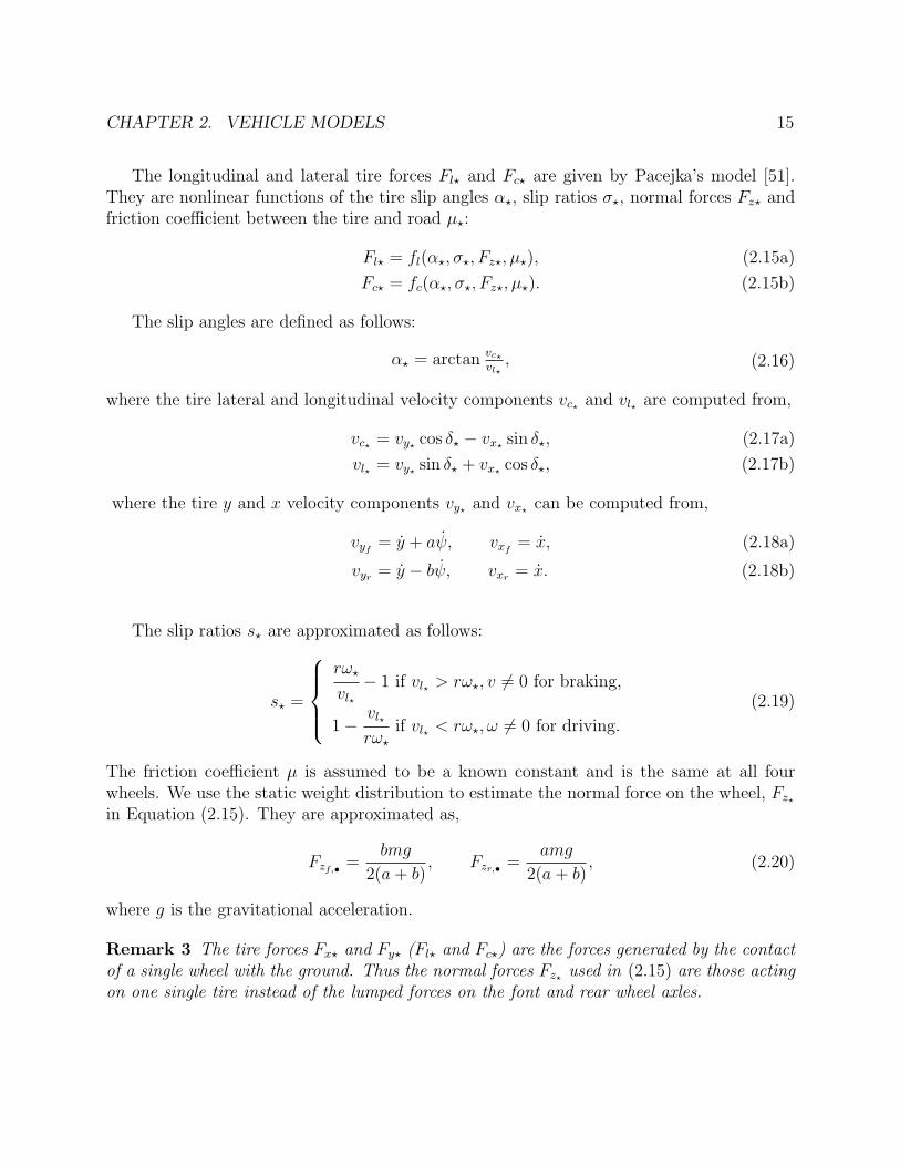
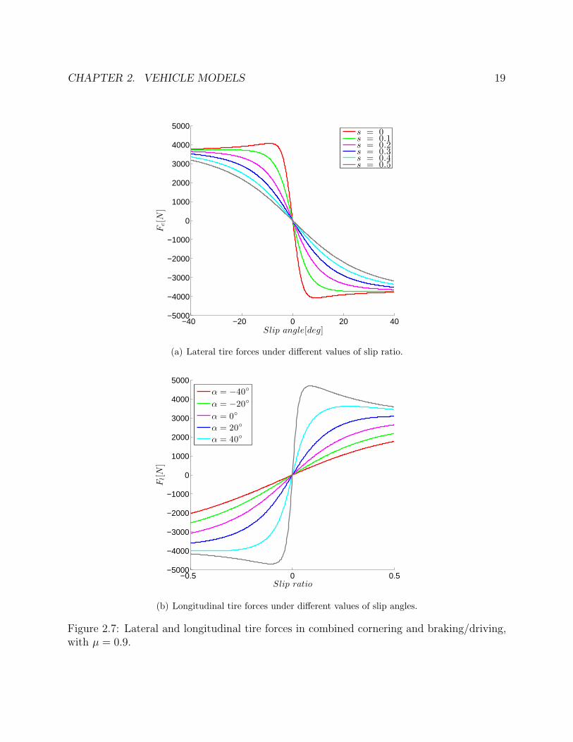
Figure 2.7 shows the longitudinal and lateral tire forces in combined cornering and brak-ing/driving, with a friction coefficient of µ = 0.9. In particular, Figure 2.7(a) shows thelateral forces as functions of slip angle at different values of slip ratio, while Figure 2.7(b)shows the longitudinal forces as functions of slip ratio at different values of slip angle.
From Figure 2.7(a), we observe that when slip ratio increases, the maximum magnitudeof lateral force decreases. We also observe decreased slop in the linear region with increasedslip ratio. The similar can be observed in the longitudinal forces as shown in Figure 2.7(b),i.e., the bigger the slip angle is, the smaller the maximum magnitude of longitudinal forceas well as the slop of the curve in the linear region are.
Figure 2.8 shows the lateral and longitudinal forces in 3-D plots, as functions of both slipangle and slip ratio.
A modified Fiala tire model for combined cornering andbraking/driving
This subsection presents a simpler version of nonlinear tire model, a modified fiala model[28], which can be used for modeling the tire lateral forces in combined cornering and brak-ing/driving condition.
This model uses αsl to denote the saturation slip angle for the lateral force and assumesthe lateral force keeps the same beyond the saturation point. The lateral force is modeledas:
fc =
−Cα tan(α) + C2
α
3ηµFz| tan(α)| tan(α)− C3
α
27η2µ2F 2ztan2(α), if|α| < αsl
−ηµFzsgn(α), if|α| ≥ αsl(2.23)
where α denotes the slip angle, µ denotes the friction coefficient, and Fz denotes the tirenormal force. Cα is a constant presenting the slop of the curve at zero slip angle. η =√µ2F 2
z − f 2l /(µFz), where fl is the longitudinal force and is treated as one of the input to
the model. The saturation slip angle is defined as follows:
CHAPTER 2. VEHICLE MODELS 19
−40 −20 0 20 40−5000
−4000
−3000
−2000
−1000
0
1000
2000
3000
4000
5000
Slip angle[deg]
Fc[N
]
s = 0s = 0.1s = 0.2s = 0.3s = 0.4s = 0.5
(a) Lateral tire forces under different values of slip ratio.
−0.5 0 0.5−5000
−4000
−3000
−2000
−1000
0
1000
2000
3000
4000
5000
Slip ratio
Fl[N
]
α = −40
α = −20
α = 0
α = 20
α = 40
(b) Longitudinal tire forces under different values of slip angles.
Figure 2.7: Lateral and longitudinal tire forces in combined cornering and braking/driving,with µ = 0.9.

CHAPTER 2. VEHICLE MODELS 20
(a) Lateral tire forces as a function of slip ratio and slip angle.
(b) Longitudinal tire forces as a function of slip ratio and slip angle.
Figure 2.8: Lateral and longitudinal tire forces as functions of slip ratio and slip angle incombined cornering and braking/driving, with µ = 0.9.

CHAPTER 2. VEHICLE MODELS 21
αsl = tan−1(3ηµFzCα
). (2.24)
We use β = fl/Fz to denote the level of braking/driving, with β = 1 denoting themaximum driving force and β = −1 denoting the maximum braking. Figure 2.9 shows thelateral forces from this model at different levels of braking/driving. Similar to the Pacejkamodel, the lateral forces show linear behavior at small values of slip angle and the maximumlateral force decreases as the braking/driving level increases. The Fiala model is less accuratethan the Pacejka model, nevertheless it captures one of the most important feature of thelateral tire dynamics, the saturation of lateral force.
−20 −10 0 10 20−5000
−4000
−3000
−2000
−1000
0
1000
2000
3000
4000
5000
Slip angle[deg]
Fc[N
]
|β| = 0|β| = 0.2|β| = 0.4|β| = 0.6|β| = 0.8
Figure 2.9: Lateral tire forces from the modified Fiala tire model at different levels of brak-ing/driving.
Linear tire model
This subsection presents a linear tire model, which can be used for modeling lateral tire forceinside the linear region. This model is only valid when both slip angle and slip ratio arerestricted to have small values.
With small α and s assumption, the lateral tire force is modeled as:
Fc = Cα(µ, Fz)α, (2.25)
where Cα is called the tire’s cornering stiffness coefficient and is a function of the frictioncoefficient µ and normal force Fz.
Figure 2.10 compares the lateral tire forces computed from the linear tire model and thePacejka model. The linear tire model is the simplest tire model we can possibly get andshould be implemented only with small slip angles, i.e. inside the tire linear region.

CHAPTER 2. VEHICLE MODELS 22
−20 −10 0 10 20
−4000
−3000
−2000
−1000
0
1000
2000
3000
4000
Slip angle[deg]
Fc[N
]
Pacejka modelLinear model
Figure 2.10: Linearized lateral tire forces in small slip angle region compared to Pacejkamodel, with s = 0 and µ = 0.9.
2.5 Linear Bicycle Model
In this section we present a linear bicycle model derived from the model (2.13). The modelis based on a linear tire model, small angle assumption and constant velocity assumption.This model is useful for some cases of lateral dynamics control during which the changesof the vehicle’s longitudinal velocity is small and not critical. We first make the followingassumption:
Assumption 3 The vehicle travels at a constant longitudinal velocity. i.e. x = 0.
The linear tire model presented in the previous section is used to model the lateral tireforce:
Fc⋆ = C⋆(µ, Fz⋆) · α⋆, (2.26)
where C⋆ is the tire’s cornering stiffness coefficient and is a function of the friction coefficientµ and normal force Fz⋆ . We assume µ is a know constant and use (2.20) to estimate thenormal force. The constant C⋆ then can be estimated according to the Pacejka tire modelwith the given µ and normal force.
To derive a linear model of the y component of tire force Fy, consider the Equations(2.14b) (2.16) and (2.18). With small angle assumption (δ⋆ < 10), we approximate sin δ⋆and cos δ⋆ using their first order Taylor expansion:
sin δ⋆ ≃ δ⋆, cos δ⋆ ≃ 1. (2.27)
Combining Equations (2.16) (2.17) and (2.27), we can express the slip angle α⋆ as:

CHAPTER 2. VEHICLE MODELS 23
α⋆ ≃vy⋆ − vx⋆δ⋆vy⋆δ⋆ + vx⋆
, (2.28)
Assuming vy ≪ vx (i.e. small side slip angle), Equation (2.28) can be approximated as:
α⋆ ≃vy⋆vx⋆− δ⋆. (2.29)
With the assumption δr = 0 and equation (2.18), we have:
αf ≃vy + aψ
vx− δf , (2.30a)
αr ≃vy − bψvx
. (2.30b)
Combining Equations (2.26) and (2.30), the lateral tire forces are computed as:
Fcf ≃ Cf · (vy + aψ
vx− δf ), (2.31a)
Fcr ≃ Cr · (vy − bψvx
). (2.31b)
With the linear tire model (2.26) and small angle assumption, we approximate Equation(2.14b) as:
Fy⋆ = Fl⋆δ⋆ + Fc⋆ ≃ Fc⋆ . (2.32a)
Substitute (2.32) into (2.13) and neglect longitudinal dynamics x, we have the followinglinear dynamic equations:
my = −mxψ + 2[Cf (vy + aψ
vx− δf ) + Cr
vy − bψvx
], (2.33a)
Iψ = 2aCf (vy + aψ
vx− δf )− 2bCr(
vy − bψvx
), (2.33b)
eψ = ψ − ψd, (2.33c)
s = x, (2.33d)
ey = x(eψ) + y. (2.33e)
Note that we used the reference framework two as in (2.3) and assumed x to be a constant.This model is compactly written as:
ξ(t) = f lin(ξ(t), u(t)) (2.34)
where the state and input vectors are ξ = [y, ψ, eψ, s, ey]′ and u = [δf ], respectively.

CHAPTER 2. VEHICLE MODELS 24
2.6 Point Mass Model
This section presents the most simplified model for the vehicle dynamics, the point massmodel. It is based on the following simplification:
Simplification 2 The vehicle is treated as a point with a given mass. The yaw dynamicsare neglected since there is no vehicle orientation can be defined. x and y direction are setto be the same as X and Y direction. The front and rear tire forces are treated together andpresented by forces in x and y directions, Fx and Fy.
With Simplification 2, the point mass model dynamic equations can be given as follows:
mx = Fx, (2.35a)
my = Fy, (2.35b)
X = x, (2.35c)
Y = y. (2.35d)
The maximum tire forces can be constrained by the friction circle:
F 2x + F 2
y ≤ (µmg)2, (2.36a)
where µ is assumed a known constant, m is the vehicle’s mass and g is the gravitationalacceleration.
The dynamics in (2.35) is compactly written as:
ξ(t) = fPM(ξ(t), u(t)) (2.37)
where the state and input vectors are ξ = [y, x, Y,X]′ and u = [Fx, Fy]′, respectively.
The point mass model is oversimplified. Besides its incapability of capturing the yawdynamics and vehicle orientation, it also fails to capture the state dependant nature of thetire forces. For instance, when starting a turn from zero yaw rate and side slip, the rear tirelateral forces need time to build up with the increase of the yaw rate and side slip. Thiscoupling of tire forces and vehicle states is not modeled in the point mass model.
Remark 4 The point mass model given by (2.35) and (2.36) is an oversimplification of themodels presented previously in this Chapter. Nevertheless, the constraint (2.36) captures oneof the most important features of the tire forces that can be generated with a given surfaceand normal force.
2.7 Concluding Remarks
Different vehicle models and tire models are presented in this Chapter, from a relativelycomplex four wheel model with Pacejka tire model to the simplest point mass model with
CHAPTER 2. VEHICLE MODELS 25
no tire model but only a friction circle constraint on tire forces. These models vary intheir accuracy and complexity and poses one important trade off in the model based vehiclecontroller design as will be shown later in this thesis. Higher fidelity models usually limitthe prediction horizon and sampling time of the MPC controller which limits the controllerperformance. Low fidelity models, on the other hand, allow large prediction horizon withsmall sampling time but can exhibit poor controller performance due to their large modelmismatch.

26
Chapter 3
Hierarchical Model Predictive Control
3.1 Introduction
Parallel advances in theory and computing systems have enlarged the range of applicationswhere real-time MPC can be applied [7, 8, 31, 22, 64, 13]. Yet, for a wide class of fastapplications, the computational burden of Nonlinear MPC (NMPC) is still a barrier. In [9]an NMPC has been implemented on a passenger vehicle for path following via an ActiveFront Steering (AFS) system at 20 Hz, by using the state of the art optimization solversand rapid prototyping systems. It is shown that the real-time execution is limited to lowvehicle speeds on icy roads, because of its computational complexity. In order to decrease thecomputational complexity, in [15, 20] a Linear Time Varying MPC approach is presented totackle the same problem. Experimental results [20, 21, 14, 16] demonstrated the capabilityof the controller to stabilize the vehicle and follow a reference trajectory at higher speeds.
Following the previous works, in this chapter, we will first compare two approaches tothe autonomous obstacle avoidance problem. In the first approach, we use the formulationin [19] and modify the cost function by adding a distance-based cost term which increasesas the vehicle gets closer to the obstacle. In the second approach, the controller design isdecomposed into two levels. The high-level uses a simplified point-mass vehicle model andreplans the path based on information about the current position of the obstacle. This isdone in a receding horizon fashion with an NMPC controller. The trajectory is fed to thelow-level controller which is formulated as the one in [19]. We compare performance andcomputation time of both approaches by using simulation and experimental results.
After concluding that the hierarchical approach is more promising and suitable for real-time implementation, we then propose a hierarchical approach for semi-autonomous obstacleavoidance. The high level path planner utilizes a special kind of curve, the clothoid, toplan the smoothest path avoiding the obstacle. A few parameters is used to determine theplanned path, which is obstacle free and feasible for the vehicle to track. That results inlow computational complexity for the high level path planner. The parameters also gives ameasure of the aggressiveness of the avoiding maneuver, providing a suitable indication of
CHAPTER 3. HIERARCHICAL MODEL PREDICTIVE CONTROL 27
whether an intervention from the controller is needed to keep the vehicle safe.This chapter is structured as follows. First, we briefly summarize the dynamics models
used in the controller, then outline the control architecture of the two approaches. We thendiscuss about the MPC formulation of the two approaches and explain how we formulate thecost term associated with obstacle avoidance. Simulation and experimental results are thenpresented, followed by discussion on the comparisons between the two approaches. At thelast part, the clothoid based semi-autonomous hierarchical controller is proposed, includingthe introduction of clothoid, the controller formulation and the simulation and experimentalresults.
3.2 Vehicle Model Summary
In this chapter, two vehicle models from Chapter 2 will be used: the Four Wheel Modeland the Point-Mass Model. The ten state nonlinear four wheel model (2.4) which includesthe longitudinal and lateral vehicle dynamics as well as wheel rotating dynamics is used forsimulating the vehicle dynamics in close loop simulations. In controller design, a six statefour wheel vehicle model is used instead, where the wheel dynamics are neglected.
Four wheel model
We use the six state four wheel vehicle model:
my = −mxψ + Fyf,l + Fyf,r + Fyr,l + Fyr,r (3.1a)
mx = myψ + Fxf,l + Fxf,r + Fxr,l + Fxr,r (3.1b)
Iψ = a(Fyf,l + Fyf,r)− b(Fyr,l + Fyr,r)+
+ c(−Fxf,l + Fxf,r − Fxr,l + Fxr,r) (3.1c)
Y = x sinψ + y cosψ (3.1d)
X = x cosψ − y sinψ (3.1e)
Details of the model can be found in Chapter 2. Note that the wheel dynamics are neglectedas discussed in Remark 1. The model is compactly written as:
ξ(t) = f 4ws(ξ(t), u(t)) (3.2)
where the superscript 4ws stands for “four wheel simplified”. The state and input vectorsare ξ = [y, x, ψ, ψ, Y,X] and u = [δf , Tf,l, Tf,r, Tr,l, Tr,r].
Point-mass model
Consider the point mass model (2.37) and assume that the longitudinal velocity of the vehicleto be constant. We define the point mass model as follows:
y = ay (3.3a)

CHAPTER 3. HIERARCHICAL MODEL PREDICTIVE CONTROL 28
x = 0 (3.3b)
ψ =ayx
(3.3c)
Y = x sinψ + y cosψ (3.3d)
X = x cosψ − y sinψ (3.3e)
|ay| < µg (3.3f)
where ψ is defined as the direction of vehicle speed and the maximum lateral accelerationay is bounded by µg. The dynamics of the point-mass model are compactly written as,
ξ(t) = f pm(ξ(t), u(t)) (3.4a)
|u(t)| < µg (3.4b)
where ξ = [y, x, ψ, Y, X]′ and u = ay.
3.3 MPC Control Architectures for An Obstacle
Avoiding Path Replanner on Slippery Surface
Control goal
In the next few sections we explore two different control architectures for an obstacle avoidingpath replan controller. The controller follows a predefined double lane change maneuver andat the same time avoids a pop up obstacle on its way by replanning the path around theobstacle. Figure 3.3 shows the reference trajectory for Y and ψ. The goal is to replan andexecute the obstacle avoiding maneuver at high speed on low friction snow tracks.
The Y and ψ references in Figure 3.3 is generated by the following equations as functionsof X:
Yref (X) =dy12(1 + tanh(z1))−
dy22(1 + tanh(z2)), (3.5a)
ψref (X) = arctan(dy1(1
cosh(z1))2(
1.2
dx1)− dy2(
1
cosh(z2))2(
1.2
dx2)), (3.5b)
where z1 = 2.425(X − 27.19) − 1.2, z2 = 2.4
21.95(X − 56.46) − 1.2, dx1 = 25, dx2 = 21.95,
dy1 = 4.05, dy2 = 5.7.
Control architectures
We compare two control architectures in this chapter. The first one is shown in Figure 3.2(a),and is referred to as one-level MPC. It uses the four wheel model presented in previoussection. The desired trajectory [xref , ψref (X), ψref (X), Yref (X)] along with the obstacleposition are fed to the control algorithm. The predictive control scheme computes the

CHAPTER 3. HIERARCHICAL MODEL PREDICTIVE CONTROL 29
0 20 40 60 80 100 120−2
0
2
4
Yref[m
]
0 20 40 60 80 100 120−0.4
−0.2
0
0.2
0.4
X[m]
ψref[rad]
Figure 3.1: Reference state trajectory of the double lane change path to be followed.
optimal inputs to safely avoid the obstacle while trying to track the desired trajectory. Notethat the forces Tbl and Tbr computed by the MPC are distributed to the braking torques,Tb⋆,• , on the four wheels by using a braking logic. Details about the braking logic can befound in [19].
The second approach is shown in Figure 3.2(b), and is referred to as two-level MPC.It is based on a hierarchical decomposition to the control problem. The desired trajec-tory [Yref (X), xref ] and obstacle position are fed to the high-level path replanner. Thepath replanner replans a path which avoids the obstacle and tracks the reference, usingthe point-mass model presented in Section Point-Mass Model. The replanned path[xref , ψrepl(X), ψrepl(X), Yrepl(X)] is then passed to a low-level path follower. The path fol-lower computes the optimal input to follow the new trajectory, using the four wheel vehiclemodel presented in section Four Wheel Model. The same braking logic as in the one-level MPC is used here. Both controllers are NMPCs and are described in detail in the nextsection.

CHAPTER 3. HIERARCHICAL MODEL PREDICTIVE CONTROL 30
BRAKING
LOGIC
ON LINE
NMPC VEHICLE
fδ
)(Xrefψ&
ξ
ξlfbT
,
rfbT
,
lrbT
,
rrbT
,
)(XYref
MPC Controller
lbF
rbF
refx&)(Xrefψ
Obstacle Position
ξ
(a) Architecture of one-level MPC. The four wheel vehicle model is used.
refx&
ξ
BRAKING
LOGIC
ON LINE
NMPC VEHICLEξlfb
T,
rfbT
,
lrbT
,
rrbT
,
)(XYreflb
F
rbF
High-Level
Path
Replanner
Obstacle
avoiding
Obstacle
Position
Low-Level Path Follower
)(Xreplψ&
)(XYrepl
refx&
)(Xreplψ
ξ
ξ
fδ
(b) Architecture of two-level MPC. The point-mass vehicle model is used forhigh-level path replanner. While the four wheel vehicle model is used for thelow-level path follower.
Figure 3.2: Two different architectures of controller design.
3.4 MPC Controller Formulation
General NMPC formulation
To formulate the MPC controller as a finite dimensional optimization problem, we discretizethe vehicle dynamics ξ = f ∗(ξ, u) with a sampling time Ts:
ξ(k + 1) = f ⋆d (ξ(k), u(k)), (3.6a)
u(k) = u(k − 1) + ∆u(k), (3.6b)
where f ∗ can be any continuous vehicle dynamics. Note we will use the change rate ofinputs ∆u as optimization variable.

CHAPTER 3. HIERARCHICAL MODEL PREDICTIVE CONTROL 31
The MPC controller can be formulated as a general optimization problem:
min∆Ut
JN(ξt, Ut,∆Ut) (3.7a)
subj. to ξk+1,t = f(ξk,t, uk,t) k = t, ..., t+Hp − 1, (3.7b)
∆uk+1,t = uk+1,t − uk,t k = t, ..., t+Hc − 1, (3.7c)
∆u(k) = 0 k = t+Hc + 1, ..., t+Hp − 1, (3.7d)
ξk,t ∈ Ξ k = t+ 1, ..., t+Hp − 1, (3.7e)
uk,t ∈ U k = t, ..., t+Hp − 1, (3.7f)
∆uk,t ∈ ∆U k = t+ 1, ..., t+Hp − 1, (3.7g)
ξt,t = ξ(t), (3.7h)
where ξt = [ξt,t , ξt+1,t , ..., ξt+Hp−1,t] is the sequence of states ξt ∈ RnHp over the predictionhorizon Hp predicted at time t, and updated according to the discretized dynamics of thevehicle model (3.7b), and uk,t and ∆uk,t ∈ Rmr is the kth vector of the input sequenceUt ∈ RmrHp and ∆Ut ∈ Rmr(Hp−1) respectively,
Ut = [u′t,t , u′t+1,t , ..., u
′t+Hc−1,t , u
′t+Hc,t , ..., u
′t+Hp−1,t]
′ (3.8a)
∆Ut = [∆u′t+1,t, ...,∆u′t+Hc−1,t,∆u
′t+Hc,t, ...,∆u
′t+Hp−1,t]
′ (3.8b)
We reduce the computational complexity of the MPC problem by holding the last Hp −Hc
input vectors in Ut constant and equal to the vector ut+Hc−1,t. With this assumption, onlythe first Hc input vectors constitutes the optimization variables. We refer to Hp as theprediction horizon and Hc as the control horizon.
At each time step t, the performance index JN(ξt, Ut,∆Ut) is optimized under the con-straints (3.7c)-(3.7g) starting from the state ξt,t = ξ(t) to obtain an optimal control sequence,U∗t = [u∗t,t
′, ..., u∗t+Hp−1,t′]′. The first of such optimal moves u∗t,t is the control action applied
to the vehicle at time t. At time t+1, a new optimization is solved over a shifted predictionhorizon starting from the new measured state ξt+1,t+1 = ξ(t+1). The time interval betweentime step t+ 1 and and time step t is the sampling time Ts.
Obstacle avoidance cost
The cost for obstacle avoidance is based on the distance between the front of the vehicleand the obstacle [62]. Assuming information on the position of the obstacle is given attime t as a collection of N discretized points, the position of the jth point is denoted asPt,j = (pXt,j
, pYt,j), j = 1, 2, ..., N . If these points are given in the inertial frame, they aretransformed to the vehicle body frame by,
pxk,t,j = (pYt,j − Yk,t) sinψk,t + (pXt,j−Xk,t) cosψk,t (3.9a)
pyk,t,j = (pYt,j − Yk,t) cosψk,t − (pXt,j−Xk,t) sinψk,t (3.9b)
CHAPTER 3. HIERARCHICAL MODEL PREDICTIVE CONTROL 32
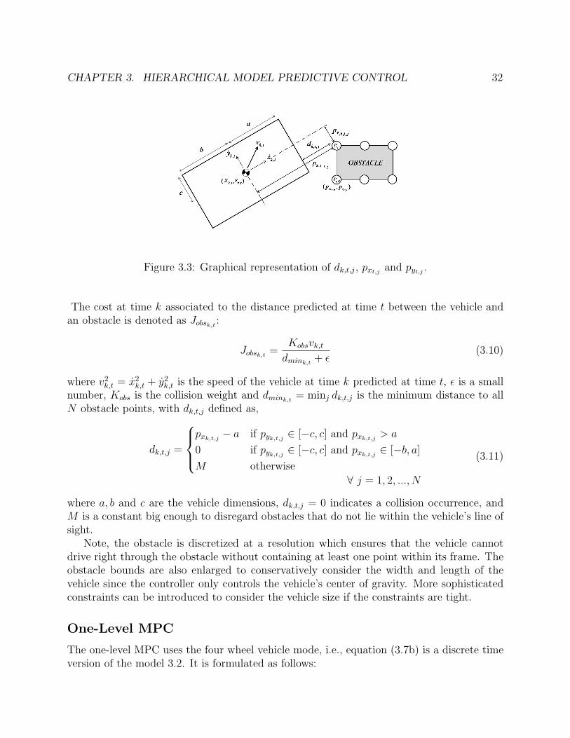
Figure 3.3: Graphical representation of dk,t,j, pxt,j and pyt,j .
The cost at time k associated to the distance predicted at time t between the vehicle andan obstacle is denoted as Jobsk,t :
Jobsk,t =Kobsvk,tdmink,t
+ ϵ(3.10)
where v2k,t = x2k,t + y2k,t is the speed of the vehicle at time k predicted at time t, ϵ is a smallnumber, Kobs is the collision weight and dmink,t
= minj dk,t,j is the minimum distance to allN obstacle points, with dk,t,j defined as,
dk,t,j =
pxk,t,j − a if pyk,t,j ∈ [−c, c] and pxk,t,j > a
0 if pyk,t,j ∈ [−c, c] and pxk,t,j ∈ [−b, a]M otherwise
∀ j = 1, 2, ..., N
(3.11)
where a, b and c are the vehicle dimensions, dk,t,j = 0 indicates a collision occurrence, andM is a constant big enough to disregard obstacles that do not lie within the vehicle’s line ofsight.
Note, the obstacle is discretized at a resolution which ensures that the vehicle cannotdrive right through the obstacle without containing at least one point within its frame. Theobstacle bounds are also enlarged to conservatively consider the width and length of thevehicle since the controller only controls the vehicle’s center of gravity. More sophisticatedconstraints can be introduced to consider the vehicle size if the constraints are tight.
One-Level MPC
The one-level MPC uses the four wheel vehicle mode, i.e., equation (3.7b) is a discrete timeversion of the model 3.2. It is formulated as follows:
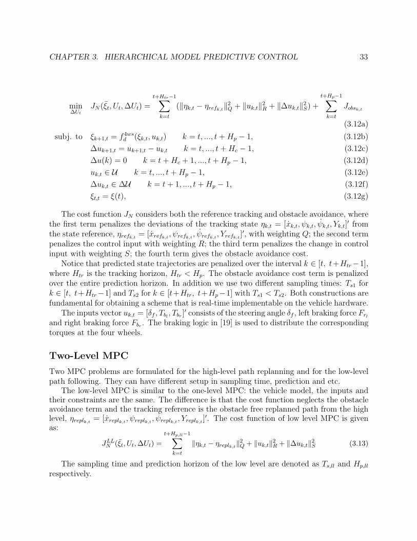
CHAPTER 3. HIERARCHICAL MODEL PREDICTIVE CONTROL 33
min∆Ut
JN(ξt, Ut,∆Ut) =t+Htr−1∑k=t
(∥ηk,t − ηrefk,t∥2Q + ∥uk,t∥2R + ∥∆uk,t∥2S) +t+Hp−1∑k=t
Jobsk,t
(3.12a)
subj. to ξk+1,t = f 4wsd (ξk,t, uk,t) k = t, ..., t+Hp − 1, (3.12b)
∆uk+1,t = uk+1,t − uk,t k = t, ..., t+Hc − 1, (3.12c)
∆u(k) = 0 k = t+Hc + 1, ..., t+Hp − 1, (3.12d)
uk,t ∈ U k = t, ..., t+Hp − 1, (3.12e)
∆uk,t ∈ ∆U k = t+ 1, ..., t+Hp − 1, (3.12f)
ξt,t = ξ(t), (3.12g)
The cost function JN considers both the reference tracking and obstacle avoidance, wherethe first term penalizes the deviations of the tracking state ηk,t = [xk,t, ψk,t, ψk,t, Yk,t]
′ fromthe state reference, ηrefk,t = [xrefk,t , ψrefk,t , ψrefk,t , Yrefk,t ]
′, with weighting Q; the second termpenalizes the control input with weighting R; the third term penalizes the change in controlinput with weighting S; the fourth term gives the obstacle avoidance cost.
Notice that predicted state trajectories are penalized over the interval k ∈ [t, t+Htr−1],where Htr is the tracking horizon, Htr < Hp. The obstacle avoidance cost term is penalizedover the entire prediction horizon. In addition we use two different sampling times: Ts1 fork ∈ [t, t+Htr−1] and Ts2 for k ∈ [t+Htr, t+Hp−1] with Ts1 < Ts2. Both constructions arefundamental for obtaining a scheme that is real-time implementable on the vehicle hardware.
The inputs vector uk,t = [δf , Tbl , Tbr ]′ consists of the steering angle δf , left braking force Frl
and right braking force Fbr . The braking logic in [19] is used to distribute the correspondingtorques at the four wheels.
Two-Level MPC
Two MPC problems are formulated for the high-level path replanning and for the low-levelpath following. They can have different setup in sampling time, prediction and etc.
The low-level MPC is similar to the one-level MPC: the vehicle model, the inputs andtheir constraints are the same. The difference is that the cost function neglects the obstacleavoidance term and the tracking reference is the obstacle free replanned path from the highlevel, ηreplk,t = [xreplk,t , ψreplk,t , ψreplk,t , Yreplk,t ]
′. The cost function of low level MPC is givenas:
JLLN (ξt, Ut,∆Ut) =
t+Hp,ll−1∑k=t
∥ηk,t − ηreplk,t∥2Q + ∥uk,t∥2R + ∥∆uk,t∥2S (3.13)
The sampling time and prediction horizon of the low level are denoted as Ts,ll and Hp,ll
respectively.

CHAPTER 3. HIERARCHICAL MODEL PREDICTIVE CONTROL 34
The high-level MPC uses the point-mass model (3.4), i.e. equation (3.7b) is a discretetime version of the model (3.4): ξ(t) = f pm(ξ(t), u(t)). The optimization problem is formu-lated as follows:
min∆Ut
JHLN (ξt, Ut) =
t+Hp,hl−1∑k=t
∥Yk,t − Yrefk,t∥2Q + ∥ayk,t∥2R + Jobsk,t (3.14a)
subj. to ξk+1,t = f pmd (ξk,t, uk,t) k = t, ..., t+Hp − 1, (3.14b)
uk,t = ut+Hc,t k = t+Hc + 1, ..., t+Hp − 1, (3.14c)
|uk,t| < µg k = t, ..., t+Hp − 1, (3.14d)
ξt,t = ξ(t), (3.14e)
The cost function JHLN weights the deviations from the lateral reference Yrefk,t , the lateralacceleration input ayk,t and the obstacle avoidance term:
JLHN (ξt, Ut) =
t+Hp,hl−1∑k=t
∥Yk,t − Yrefk,t∥2Q + ∥ayk,t∥
2R + Jobsk,t (3.15)
The sampling time and prediction horizon of the high level are denoted as Ts,hl and Hp,hl
respectively.
3.5 Simulation and Experimental Results
To test the performance of the two approaches, a series of double lane change maneuversat different entry speeds have been simulated and experimentally tested. The goal is tofollow the double lane change as closely as possible while avoiding obstacles. The desiredpath is described in terms of lateral position Yref and yaw angle ψref as a function of thelongitudinal position X, as described in section 3.3.
Simulation setup description
We use Matlabr to simulate the close loop systems. The MPC optimization problem hasbeen implemented as a C-coded s-Function. The commercial NPSOL software package [25] isused for solving the nonlinear programming problem (3.7). The first element of the optimizedcontrol sequence is passed to another external block which uses the ten state four wheel model(2.4) to simulate the dynamics of the vehicle, and feeds the current state of the vehicle backto the controller.We simulate results using this procedure to compare the computation loadsfor the two different approaches.
Experimental setup description
The two approaches presented before have been tested through experiments on slipperysurfaces. The experiments have been performed at a test center equipped with icy and

CHAPTER 3. HIERARCHICAL MODEL PREDICTIVE CONTROL 35
snowy handling tracks. The MPC controllers have been tested on a passenger car, with amass of 2050 Kg and an inertia of 3344 Kg/m2. The controllers were run in a dSPACEAutobox system, equipped with a DS1005 processor board and a DS2210 I/O board.
We used an Oxford Technical Solution (OTS) RT3002 sensing system to measure theposition and the orientation of the vehicle in the inertial frame and the vehicle velocitiesin the vehicle body frame. The OTS RT3002, is housed in a small package that contains aDifferential Global Positioning System (DGPS) receiver, Inertial Measurement Unit (IMU),and a Digital Signal Processor (DSP). It is equipped with a single antenna to receive GPSinformation. The IMU includes three accelerometers and three angular rate sensors. TheDSP receives both the measurements from the IMU and the DGPS, utilizes a Kalman filterfor sensor fusion, and calculate the position, orientation and other states of the vehicle suchas longitudinal and lateral velocities. Compared to a dual antenna setup, a single antennasystem has to learn the vehicle orientation and/or coordinate during vehicle motion. Thismight cause the presence of a small offset in the orientation measurement. In dual antennasystems the vehicle orientation can be easily set even if the vehicle is not moving.
The car was equipped with an Active Front Steering (AFS) and Differential Brakingsystem which utilizes an electric drive motor to change the relation between the hand steeringwheel and road wheel angles. This is done independently from the hand wheel position, thusthe front road wheel angle is obtained by summing the driver hand wheel position and theactuator angular movement. Both the hand wheel position and the angular relation betweenhand and road wheels are measured.
This steering actuator can operate in two modes: with and without the intervention ofthe controller. In the first mode the steering commands of the controller and the driveroverlap and the overall steering action is the results of the contributions from the driver andthe controller. In the second mode there is not controller intervention and the steering angleis completely decided by the driver through the steering wheel. We used the second mode,and the driver action represents an input disturbance. The sensor, the dSPACE Autoboxand the actuators communicate through a CAN bus.
The test is initiated by the driver with a button. When the button is pushed, the inertialframe in Figure 2.2(a) is initialized as follows: the origin is the current vehicle position, theaxes X and Y are directed as the current longitudinal and lateral vehicle axes, respectively.Such inertial frame becomes also the desired path coordinate system. Once the initializationprocedure is concluded, the vehicle executes the double lane change and obstacle avoidancemaneuver.
Note that, noise may affect the yaw angle measurement due to the single antenna sensorsetup. Compared to a dual antenna setup, a single antenna system has to learn the vehicleorientation and/or coordinate during vehicle motion. When the vehicle stands still the yawangle is computed by integrating the yaw rate measurement from the IMU. This might causethe presence of a small offset in the orientation measurement, while traveling at low speedor being still.
A photo of the test vehicle is shown in Figure 3.4.
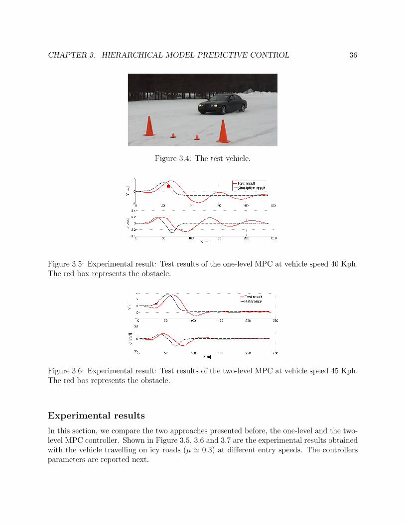
CHAPTER 3. HIERARCHICAL MODEL PREDICTIVE CONTROL 36
Figure 3.4: The test vehicle.
Figure 3.5: Experimental result: Test results of the one-level MPC at vehicle speed 40 Kph.The red box represents the obstacle.
Figure 3.6: Experimental result: Test results of the two-level MPC at vehicle speed 45 Kph.The red bos represents the obstacle.
Experimental results
In this section, we compare the two approaches presented before, the one-level and the two-level MPC controller. Shown in Figure 3.5, 3.6 and 3.7 are the experimental results obtainedwith the vehicle travelling on icy roads (µ ≃ 0.3) at different entry speeds. The controllersparameters are reported next.

CHAPTER 3. HIERARCHICAL MODEL PREDICTIVE CONTROL 37
Figure 3.7: Experimental result: Test results of the two-level MPC at vehicle speed 55 Kph.The red box represents the obstacle.
Figure 3.8: Experimental result: Replanned paths from the high-level path replanner intwo-level MPC. Vehicle speed is 55 Kph.
Tuning 1A One-level MPC: Nonlinear MPC (3.12) with model (3.2) and cost (3.12a) andwith the following parameters
• Ts1 = 0.1s, Ts2 = 0.3s, Hp = 10, Hc = 2, Htr = 5
• δf ∈ [−10 , 10 ], ∆δf ∈ [−17 , 17 ]× Ts1
• Fb• ∈ [−1500, 0], ∆Fb• ∈ [−1000, 1000]× Ts1
• Q = diag(10−2, 1, 1, 30), R = diag(10, 1, 1)S = diag(10−2, 1, 1), Kobs = 1
Tuning 2HL Hierarchical MPC High-level: Nonlinear MPC (3.14) with model (3.4) andcost (3.14a) and with the following parameters.
• Ts,hl = 0.1s, Hp,hl = 15; Hc = 2
• ay ∈ [−µg, µg]
• Q = 10, R = 12, Kobs = 1
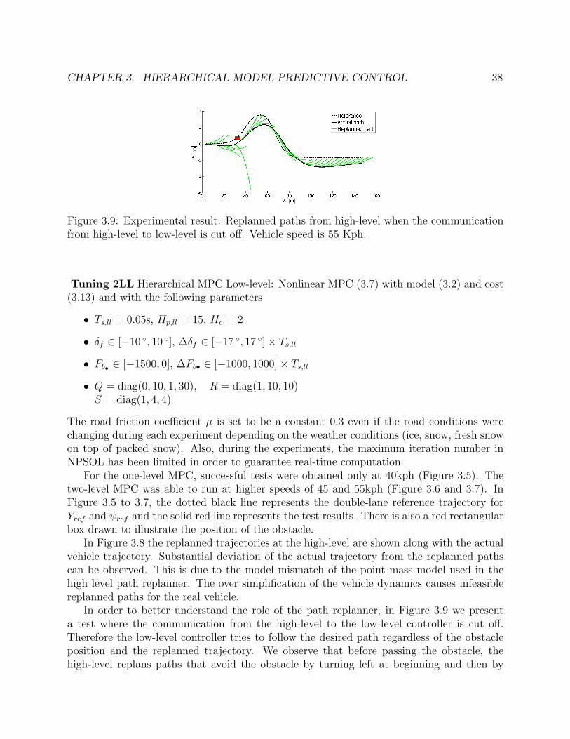
CHAPTER 3. HIERARCHICAL MODEL PREDICTIVE CONTROL 38
Figure 3.9: Experimental result: Replanned paths from high-level when the communicationfrom high-level to low-level is cut off. Vehicle speed is 55 Kph.
Tuning 2LL Hierarchical MPC Low-level: Nonlinear MPC (3.7) with model (3.2) and cost(3.13) and with the following parameters
• Ts,ll = 0.05s, Hp,ll = 15, Hc = 2
• δf ∈ [−10 , 10 ], ∆δf ∈ [−17 , 17 ]× Ts,ll
• Fb• ∈ [−1500, 0], ∆Fb• ∈ [−1000, 1000]× Ts,ll
• Q = diag(0, 10, 1, 30), R = diag(1, 10, 10)S = diag(1, 4, 4)
The road friction coefficient µ is set to be a constant 0.3 even if the road conditions werechanging during each experiment depending on the weather conditions (ice, snow, fresh snowon top of packed snow). Also, during the experiments, the maximum iteration number inNPSOL has been limited in order to guarantee real-time computation.
For the one-level MPC, successful tests were obtained only at 40kph (Figure 3.5). Thetwo-level MPC was able to run at higher speeds of 45 and 55kph (Figure 3.6 and 3.7). InFigure 3.5 to 3.7, the dotted black line represents the double-lane reference trajectory forYref and ψref and the solid red line represents the test results. There is also a red rectangularbox drawn to illustrate the position of the obstacle.
In Figure 3.8 the replanned trajectories at the high-level are shown along with the actualvehicle trajectory. Substantial deviation of the actual trajectory from the replanned pathscan be observed. This is due to the model mismatch of the point mass model used in thehigh level path replanner. The over simplification of the vehicle dynamics causes infeasiblereplanned paths for the real vehicle.
In order to better understand the role of the path replanner, in Figure 3.9 we presenta test where the communication from the high-level to the low-level controller is cut off.Therefore the low-level controller tries to follow the desired path regardless of the obstacleposition and the replanned trajectory. We observe that before passing the obstacle, thehigh-level replans paths that avoid the obstacle by turning left at beginning and then by
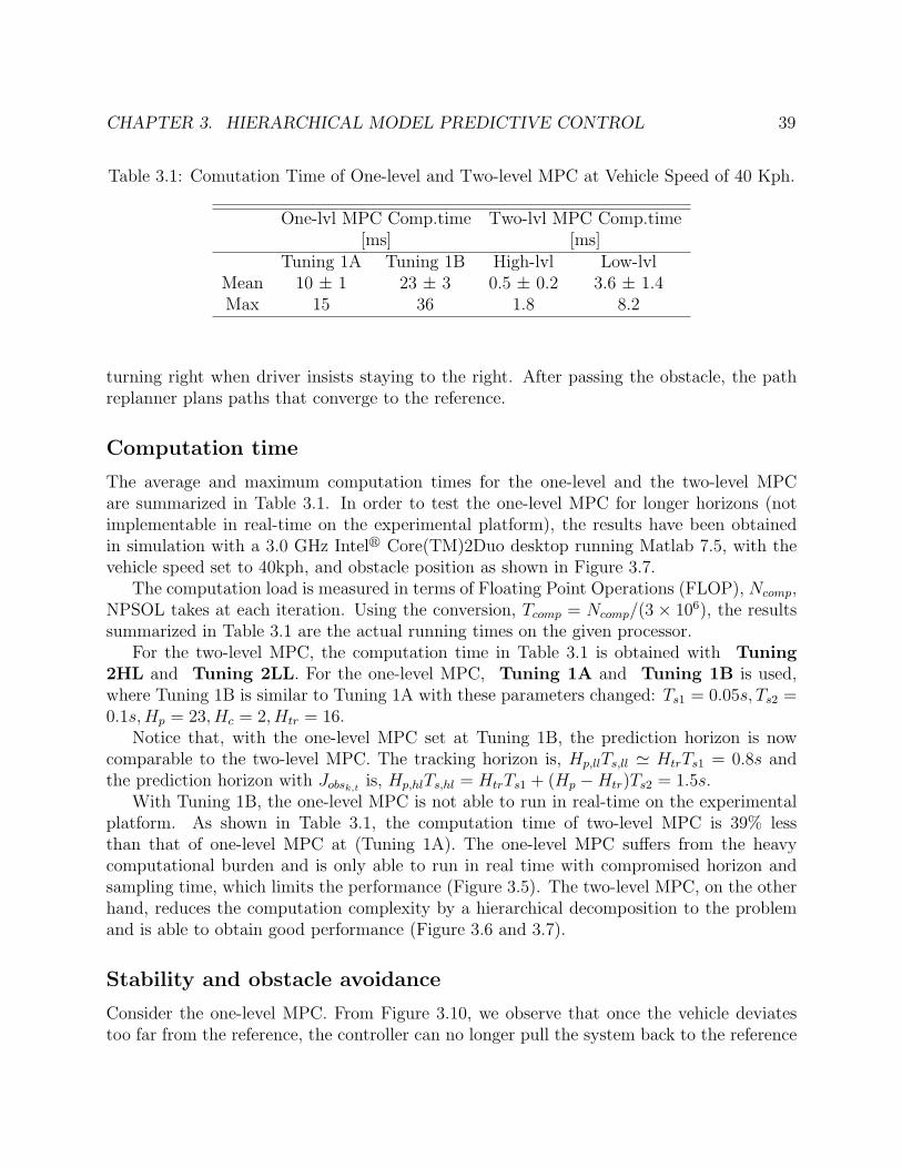
CHAPTER 3. HIERARCHICAL MODEL PREDICTIVE CONTROL 39
Table 3.1: Comutation Time of One-level and Two-level MPC at Vehicle Speed of 40 Kph.
One-lvl MPC Comp.time Two-lvl MPC Comp.time[ms] [ms]
Tuning 1A Tuning 1B High-lvl Low-lvlMean 10 ± 1 23 ± 3 0.5 ± 0.2 3.6 ± 1.4Max 15 36 1.8 8.2
turning right when driver insists staying to the right. After passing the obstacle, the pathreplanner plans paths that converge to the reference.
Computation time
The average and maximum computation times for the one-level and the two-level MPCare summarized in Table 3.1. In order to test the one-level MPC for longer horizons (notimplementable in real-time on the experimental platform), the results have been obtainedin simulation with a 3.0 GHz Intelr Core(TM)2Duo desktop running Matlab 7.5, with thevehicle speed set to 40kph, and obstacle position as shown in Figure 3.7.
The computation load is measured in terms of Floating Point Operations (FLOP), Ncomp,NPSOL takes at each iteration. Using the conversion, Tcomp = Ncomp/(3 × 106), the resultssummarized in Table 3.1 are the actual running times on the given processor.
For the two-level MPC, the computation time in Table 3.1 is obtained with Tuning2HL and Tuning 2LL. For the one-level MPC, Tuning 1A and Tuning 1B is used,where Tuning 1B is similar to Tuning 1A with these parameters changed: Ts1 = 0.05s, Ts2 =0.1s,Hp = 23, Hc = 2, Htr = 16.
Notice that, with the one-level MPC set at Tuning 1B, the prediction horizon is nowcomparable to the two-level MPC. The tracking horizon is, Hp,llTs,ll ≃ HtrTs1 = 0.8s andthe prediction horizon with Jobsk,t is, Hp,hlTs,hl = HtrTs1 + (Hp −Htr)Ts2 = 1.5s.
With Tuning 1B, the one-level MPC is not able to run in real-time on the experimentalplatform. As shown in Table 3.1, the computation time of two-level MPC is 39% lessthan that of one-level MPC at (Tuning 1A). The one-level MPC suffers from the heavycomputational burden and is only able to run in real time with compromised horizon andsampling time, which limits the performance (Figure 3.5). The two-level MPC, on the otherhand, reduces the computation complexity by a hierarchical decomposition to the problemand is able to obtain good performance (Figure 3.6 and 3.7).
Stability and obstacle avoidance
Consider the one-level MPC. From Figure 3.10, we observe that once the vehicle deviatestoo far from the reference, the controller can no longer pull the system back to the reference
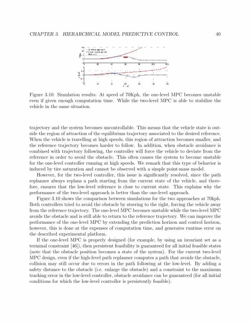
CHAPTER 3. HIERARCHICAL MODEL PREDICTIVE CONTROL 40
Figure 3.10: Simulation results: At speed of 70Kph, the one-level MPC becomes unstableeven if given enough computation time. While the two-level MPC is able to stabilize thevehicle in the same situation.
trajectory and the system becomes uncontrollable. This means that the vehicle state is out-side the region of attraction of the equilibrium trajectory associated to the desired reference.When the vehicle is travelling at high speeds, this region of attraction becomes smaller, andthe reference trajectory becomes harder to follow. In addition, when obstacle avoidance iscombined with trajectory following, the controller will force the vehicle to deviate from thereference in order to avoid the obstacle. This often causes the system to become unstablefor the one-level controller running at high speeds. We remark that this type of behavior isinduced by tire saturation and cannot be observed with a simple point-mass model.
However, for the two-level controller, this issue is significantly resolved, since the pathreplanner always replans a path starting from the current state of the vehicle, and there-fore, ensures that the low-level reference is close to current state. This explains why theperformance of the two-level approach is better than the one-level approach.
Figure 3.10 shows the comparison between simulations for the two approaches at 70kph.Both controllers tried to avoid the obstacle by steering to the right, forcing the vehicle awayfrom the reference trajectory. The one-level MPC becomes unstable while the two-level MPCavoids the obstacle and is still able to return to the reference trajectory. We can improve theperformance of the one-level MPC by extending the prediction horizon and control horizon,however, this is done at the expenses of computation time, and generates runtime error onthe described experimental platform.
If the one-level MPC is properly designed (for example, by using an invariant set as aterminal constraint [46]), then persistent feasibility is guaranteed for all initial feasible states(note that the obstacle position becomes a state of the system). For the current two-levelMPC design, even if the high-level path replanner computes a path that avoids the obstacle,collision may still occur due to errors in the path following at the low-level. By adding asafety distance to the obstacle (i.e. enlarge the obstacle) and a constraint to the maximumtracking error in the low-level controller, obstacle avoidance can be guaranteed (for all initialconditions for which the low-level controller is persistently feasible).
CHAPTER 3. HIERARCHICAL MODEL PREDICTIVE CONTROL 41
3.6 Concluding Remarks on Control Architecture
Comparison
We have presented two MPC approaches for trajectory following for autonomous ground ve-hicles with obstacle avoidance. The one-level approach combines both requirements into onelarge finite horizon optimization problem, while the two-level approach breaks this probleminto a high-level path replanner and a low-level path follower. The experiments show suc-cessful results from the two level approach with entering speeds up to 55kph on icy surfaces.
For the one-level approach, the computation time increases at higher speeds and there-fore real-time implementation presents an issue. The high computational complexity alsolimits the prediction horizon and sampling time in the one-level approach, which limits thecontroller performance. The two-level approach shows promise in this aspect with its muchlower computational burden. However, the point mass model used in the high level is oversimplified. That results in infeasible replanned path for the real vehicle. As can be seen inFigure 3.8, the actual vehicle trajectory is not able to follow the replanned path closely.
To address the model over simplification problem in the two-level approach, we willpropose an improved approach in the next chapter.
3.7 Clothoid Based Semi-Autonomous Hierarchical
MPC for Obstacle Avoidance
In this section, we propose a hierarchical MPC with the same structure of the two-levelMPC in section 3.3. The low level is the same NMPC as in the point mass two-level con-troller. The high level is a path planner using a special curve, clothoid, to plan obstacle freepaths. Clothoids are parameterized curves suitable for constructing lane change trajectories.Later we will show its usefulness in obtaining a semi-autonomous vehicle with adjustabledegrees of autonomy.
Parameterized clothoids
A clothoid is a curve with a curvature that changes linearly with the curve length. It iswidely used in railway and high way engineering for curvature transition. Also, its use inroad design and robot path planning has a long history. Relevant references include [57, 56,37]. In a clothoid, at a given curve length s the curvature K(s) is determined by the linearfunction K(s) = 2a2 · s, where a is the curvature change rate. The clothoid is expressed bythe Fresnel integral [57] as:
X(s) =1
a
∫ aL
0
cos(s2)ds, (3.16a)

CHAPTER 3. HIERARCHICAL MODEL PREDICTIVE CONTROL 42
0 10 20 30 40 50
0
5
10
X(m)
Y(m
)
L=5.2, a=0.086
L=7.6, a=0.048
L=10.1, a=0.031
L=12.6, a=0.023
0 10 20 30 40 50−0.1
−0.05
0
0.05
0.1
Curve length (m)
Cu
rva
ture
(1
/m)
Figure 3.11: Lane change paths with different aggressiveness. Each is generated by connect-ing four pieces of clothoids. The upper figure shows the shapes of the paths in global frame.The lower figure shows the piecewise affine relation between curvature and curve length foreach path.
Y (s) =1
a
∫ aL
0
sin(s2)ds, (3.16b)
where X and Y are the global coordinates and L is the maximum curve length. In numericalcomputation schemes, the integrals in Equation (3.16) are approximated by their Taylorexpansion:
∫ aL
0
cos(s2)ds = aL− (aL)5
5× 2!+
(aL)9
9× 4!− (aL)13
13× 6!+ ..., (3.17a)∫ aL
0
sin(s2)ds =(aL)3
3− (aL)7
7× 3!+
(aL)11
11× 5!− (aL)15
15× 7!+ ..., (3.17b)
By varying the parameters a and L, different clothoids are generated. A lane-changemaneuver is built by connecting 4 pieces of clothoids together, as shown in Figure 3.11. Themaximum curvature of the clothoid defined by Equation (3.16) is 2a2L. Thus, the maximumlateral force needed to track the clothoid is mx2 · 2a2L. Thus, by constraining a and L wecan guarantee that the required lateral force is feasible.
For a point-mass model, the upper bound on lateral force is µmg. Thus, the constrainton curvature for a point-mass model is 2a2L ≤ µg
x2. For the four-wheel model described in

CHAPTER 3. HIERARCHICAL MODEL PREDICTIVE CONTROL 43
section 3.2, the maximum achievable lateral force depends on the current vehicle states. Atthe beginning of a turn where lateral velocity y and yaw rate ψ are both zero, the lateralforce at the rear tires are zero, therefore the only source of lateral force at that instant arethe front tires. We use sampling and extensive simulations of our vehicle model to determinethe maximum available lateral force at the beginning of a turn (0.46µmg). After the turnbegins, y and ψ increase and more lateral force will become available. For a conservativeapproximation, the value 0.46µmg is taken as the upper bound of lateral force along theturn. The constraint on a and L for the clothoid becomes:
2a2L ≤ 0.46µg
x2(3.18a)
where µ is the friction coefficient and x is the body-fixed longitudinal velocity.
Obstacle and safety constraints
We use scenario based ad-hoc constraints for the obstacle avoidance. Figure 3.12 shows onescenario where the vehicle takes a left lane change to avoid the obstacle which is presentedby the red box. The lane change maneuver is composed of four clothoids, indicated by 1, 2,3 and 4 in the figure. We assume 1 and 2 have the same parameters [a1, L1] and 3, 4 sharethe same parameters [a2, L2]. The final heading angle at point B is assumed to be zero forsimplification. The optimization variables for the high level are chosen to be P = [Xa, Xb, Yb].With a given P and the initial point [X0, Y0, ψ0], the parameters [a1, L1, a2, L2] as well asthe whole planned curve can be uniquely determined, including the coornidates (Xa, Xb, ψa)and (Ya, Yb, ψb).
To guarantee obstacle avoidance, we apply the following constraints on P for the scenarioin Figure 3.12:
Xa ≤ Xc, (3.19a)
Xb ≥ Xc, (3.19b)
Yb ≥ Yc, (3.19c)
(Yc − Ya) ≤ (Yb − Ya) ·Xc −Xa
Xb −Xa
, (3.19d)
where (3.19a) ensures point A is at the left side of the obstacle; (3.19b) ensures point B haspassed the left side of the obstacle; (3.19c) ensures point B is above the obstacle; (3.19d)ensures point C is at the bottom right side of the line AB. Similar constraints can beformulated under other scenarios.
The following constraints are also applied for safety:
YLB ≤ Yb ≤ YUB, (3.20a)
|ψa| ≤ π/4, (3.20b)

CHAPTER 3. HIERARCHICAL MODEL PREDICTIVE CONTROL 44
0 5 10 15 20 25 30 35 40−10
−5
0
5
10
A
B
C : (Xc, Yc)(Xa, Ya, ψa)
(Xb, Yb, ψb)
12
34
(a1, L1)
(a2, L2)
Y[m
]
X[m]
Figure 3.12: Ad-hoc Clothoid parameters setup for obstacle constraints.
K1max ≤0.46µg
x, (3.20c)
K2max ≤0.46µg
x, (3.20d)
where (3.20a) represents the road bound constraint, with YLB and YUB being the lower andupper bound of Y for the road bound, respectively; (3.20b) limits the maximum yaw angle ofthe vehicle along the planed path; (3.20c) and (3.20d) constraints the maximum curvature ofthe clothoids. K1max and K2max are functions of the optimization variable P = [Xa, Xb, Yb].
Equations (3.19) and (3.20) are compactly written as:
h(ξ0, P ) ≤ 0, (3.21a)
where 0 is the zero vector with appropriate dimension.
MPC formulation
The optimization problem for the high level path planner is formulated as follows:
minPt
JHLN (ξt,t, Pt) = K21max
+K22max
(3.22a)
subj. to h(ξt,t, Pt) ≤ 0, (3.22b)
ξt,t = ξ(t), (3.22c)
Once the optimal parameter vector P ∗ is determined, the optimal clothoid curves canbe computed and fed to the low level. The values K1max and K2max tells how aggressive themaneuver has to be in order to avoid the obstacle. Based on that, The low level MPC candetermine whether or not to intervene by taking over control and following the planned pathfrom the high level.
A similar MPC is set up to take the vehicle back into the original lane.

CHAPTER 3. HIERARCHICAL MODEL PREDICTIVE CONTROL 45
0 50 100 150 200 250 3000
5
10
15
20
X [m]
Y [m
]
Figure 3.13: Simulation result: Various lane change maneuvers are compared. As the vehicleapproaches the obstacle the planned paths become more aggressive (high curvatures).
Simulation and experimental results
In this subsection we show the simulation and experimental results of the proposed hierar-chical MPC. The simulation and experimental setups are the same as the ones described insection 3.5. The experiments have been performed at a test center equipped with icy andsnowy handling tracks.
Figure 3.13 shows three different lane change maneuvers. They are generated from thehigh-level path planner starting from X = 120, 140, and 160m. As the vehicle approachesthe obstacle, the planned paths become more aggressive, that is, the maximum curvature ofthe planned clothoids approaches the limit at the given speed and friction coefficient. Themaneuver in red is the most aggressive maneuver the vehicle can handle at the given speed.The simulations presented in Figure 3.14 use a binary driver model. The driver is eitherattentive, as in the upper plot of Figure 3.14, and the low-level controller does not assumecontrol until the planned path becomes aggressive, or the driver is distracted, as in the lowerplot of Figure 3.14, and the low-level control begins tracking the planned path with a lowerdegree of curvature.
Figure 3.15 and 3.16 show the experimental results of the semi-autonomous driving on asnow track. In the experiments, Xb in (3.19b) is set to be equal to the X coordinate of theobstacle center, for simplicity. In the first test shown in Figure 3.15 the driver was assumedto be distracted and the path tracker assumed control early enough to track a smoothlyplanned trajectory. In the second experiment in Figure 3.16 the driver was assumed to beattentive and the controller did not take over until the planned path became aggressive.Both experiments successfully avoided the obstacle.
Note that the low-level path follower might not be able to track the planned path perfectlybecause of model mismatch and external disturbances. In some cases, the tracking error islarge enough that the maneuver becomes infeasible to track. The second experiment inFigure 3.16 shows this interesting behavior. In the test, when infeasibility appeared, abraking maneuver was invoked to reduce the velocity and thus enlarge the feasible region.

CHAPTER 3. HIERARCHICAL MODEL PREDICTIVE CONTROL 46
0 50 100 150 200 250 3000
10
20
Y [m
]
Simulated path
Planned path
0 50 100 150 200 250 3000
10
20
X [m]
Y [m
]
Figure 3.14: Simulation result: In the upper plot an attentive driver is assumed. The low-level control takes over when the planned path becomes aggressive. In the lower plot thelow-level control takes over for a distracted driver and the result is a smoother and saferpath.
0 50 100 150 200−10
0
10
X(m)
Y(m)
Actual trajectory
Reference
0 50 100 150 2008
10
12
vx(m/s)
X(m)
Figure 3.15: Experimental results: Vehicle successfully avoids the obstacle using maneuversbased on clothoids.
In Fig 3.16 we can see that after a few seconds of braking the path planner is able to find afeasible solution around the obstacle, braking is interrupted and the obstacle is successfullyavoided.
CHAPTER 3. HIERARCHICAL MODEL PREDICTIVE CONTROL 47
0 50 100 150 200−10
0
10
X(m) Y(m)
Actual trajectory
Reference
Start brake
Brake released
0 50 100 150 2008
10
12
vx(m/s)
X(m)
Figure 3.16: Experimental result: Actual path of the vehicle deviates from the planned pathdue to model mismatch and caused infeasibility of tracking. Braking was invoked to enlargethe feasible region in that situation.
3.8 Concluding Remarks
In this Chapter, we first compared two control architectures for autonomous obstacle avoid-ance, the one-level approach and the two-level hierarchical approach. The one-level ap-proach is limited by its high computational complexity and is only able to control the vehi-cle at low speeds with compromised performances. While the two-level approach is morepromising thanks to its low complexity due to the decomposition of the problem into a highlevel path replanner and low level path follower. With a simple vehicle model, the highlevel is able to plan over long prediction horizon at small sampling time. The higher fidelityvehicle model used in the low level allows the low level path follower to stabilize the vehiclearound the planned path. However, due to the oversimplification of the point mass model,the high level planned path is sometimes infeasible for the real vehicle to track. Thus in thenext chapter, We will propose an improved approach with the same two level hierarchicalarchitecture.
In the last part of this chapter, We proposed a semi-autonomous obstacle avoidancehierarchical MPC based on a special kind of curve, the clothoid. Thanks to the propertiesof clothoid, we are able to plan feasible paths with only few parameters. We can determinethe aggressiveness of the planned path from the optimal parameters and based on thatdetermine the right time to intervene the vehicle control. The clothoid based hierarchicalcontroller is fast for real-time computation and performs well. However, the use of ad-hocobstacle constraints makes it hard to be extended to more generic scenarios. There is somestudy on the generic formulation utilizing the clothoids [26]. However, a mixed integernonlinear programming is required in that approach, which is not suitable for fast real-time

CHAPTER 3. HIERARCHICAL MODEL PREDICTIVE CONTROL 48
implementation.
49
Chapter 4
Spatial Model Predictive Control
4.1 Introduction
Real-time generation and tracking of feasible trajectories is a major barrier in autonomousguidance systems when the vehicle travels at the limits of its handling capability. Trajec-tories generated by using oversimplified models violate system constraints, while computingtrajectories using high-fidelity vehicle models and nonlinear optimization is computationallydemanding. Moreover, the presence of external disturbances and model uncertainties mightstill prevent the vehicle from following the desired path.
The previous chapter proposed a hierarchical two-level NMPC scheme for the autonomousand semiautonomous driving problem. The high-level path planner uses a simplified point-mass vehicle model to generate an obstacle avoiding trajectory by using a NMPC controller.The trajectory is fed to the low-level path follower designed by using a NMPC based on ahigher fidelity vehicle model. In [23] the proposed hierarchical framework has been imple-mented on an autonomous ground vehicle driving at high speeds on an icy road. Althoughthis decomposition allows for real-time implementation, the trajectories generated by thepoint-mass path planner are not always feasible. The lower level tracking performance dete-riorates and obstacle collisions can be observed in conditions where the obstacle could havebeen avoided.
In order to overcome this issue and still maintain real-time feasibility, the work in [27] usesa motion primitive path planner at the high level. Although the high level trajectories fromthe motion primitive planner are feasible for the high-fidelity model, the optimal trajectoryrequires the online solution of a mixed-integer program or the offline computation of alarge look-up table. This prevents the use of such approach on current electronic controlunits. In order to plan a feasible path in real-time this paper studies the use of spatialpredictive control at the high level. We follow the approach presented in [61, 30] andtransform time-dependent vehicle dynamics into spatial-dependent dynamics. By using thisapproach obstacle constraints are translated into spatial constraints on the state vector.Simulation and experimental results show the controller’s ability to avoid multiple obstacles
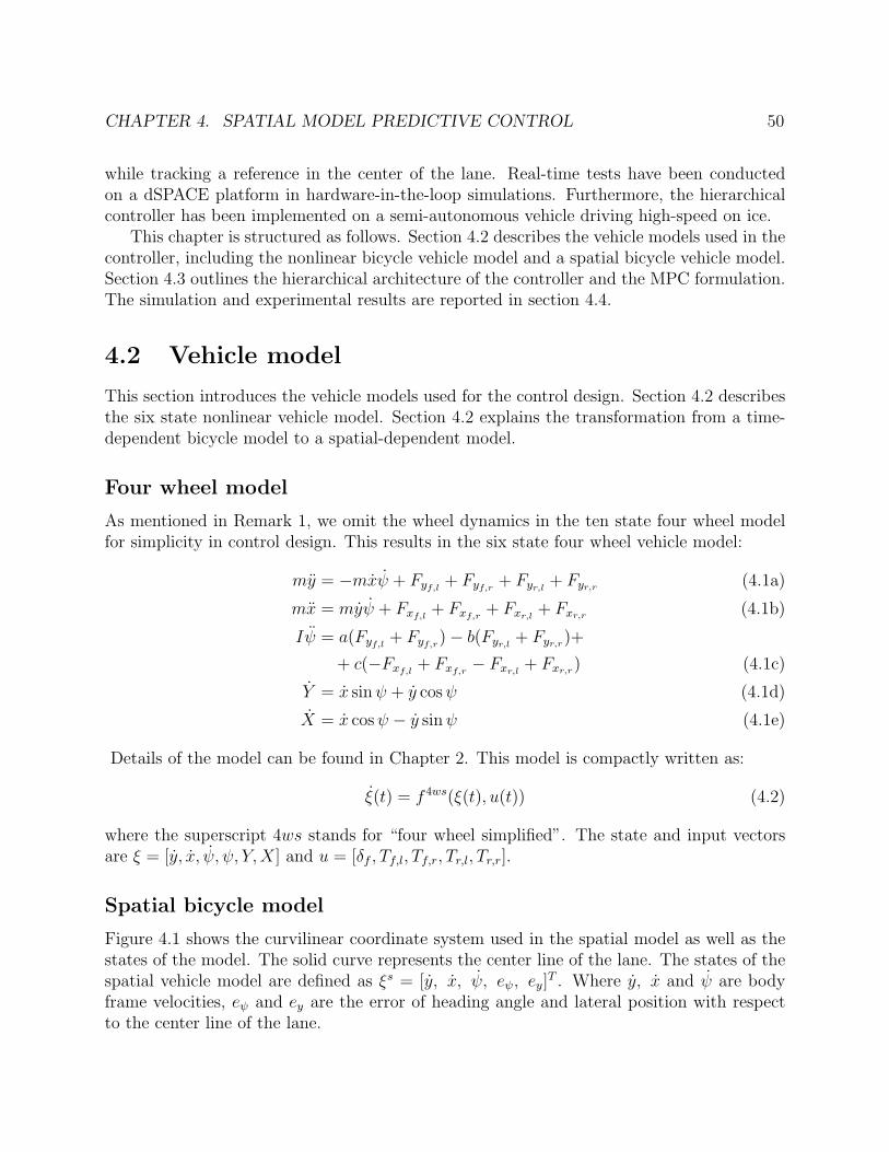
CHAPTER 4. SPATIAL MODEL PREDICTIVE CONTROL 50
while tracking a reference in the center of the lane. Real-time tests have been conductedon a dSPACE platform in hardware-in-the-loop simulations. Furthermore, the hierarchicalcontroller has been implemented on a semi-autonomous vehicle driving high-speed on ice.
This chapter is structured as follows. Section 4.2 describes the vehicle models used in thecontroller, including the nonlinear bicycle vehicle model and a spatial bicycle vehicle model.Section 4.3 outlines the hierarchical architecture of the controller and the MPC formulation.The simulation and experimental results are reported in section 4.4.
4.2 Vehicle model
This section introduces the vehicle models used for the control design. Section 4.2 describesthe six state nonlinear vehicle model. Section 4.2 explains the transformation from a time-dependent bicycle model to a spatial-dependent model.
Four wheel model
As mentioned in Remark 1, we omit the wheel dynamics in the ten state four wheel modelfor simplicity in control design. This results in the six state four wheel vehicle model:
my = −mxψ + Fyf,l + Fyf,r + Fyr,l + Fyr,r (4.1a)
mx = myψ + Fxf,l + Fxf,r + Fxr,l + Fxr,r (4.1b)
Iψ = a(Fyf,l + Fyf,r)− b(Fyr,l + Fyr,r)+
+ c(−Fxf,l + Fxf,r − Fxr,l + Fxr,r) (4.1c)
Y = x sinψ + y cosψ (4.1d)
X = x cosψ − y sinψ (4.1e)
Details of the model can be found in Chapter 2. This model is compactly written as:
ξ(t) = f 4ws(ξ(t), u(t)) (4.2)
where the superscript 4ws stands for “four wheel simplified”. The state and input vectorsare ξ = [y, x, ψ, ψ, Y,X] and u = [δf , Tf,l, Tf,r, Tr,l, Tr,r].
Spatial bicycle model
Figure 4.1 shows the curvilinear coordinate system used in the spatial model as well as thestates of the model. The solid curve represents the center line of the lane. The states of thespatial vehicle model are defined as ξs = [y, x, ψ, eψ, ey]
T . Where y, x and ψ are bodyframe velocities, eψ and ey are the error of heading angle and lateral position with respectto the center line of the lane.
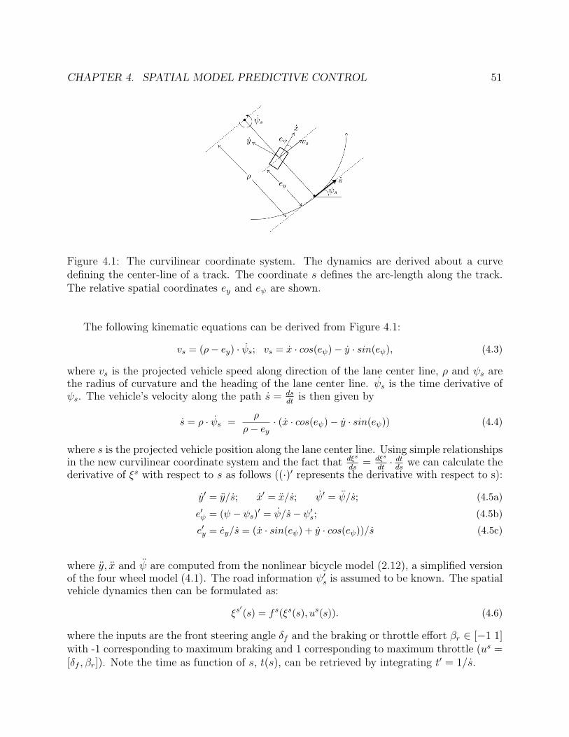
CHAPTER 4. SPATIAL MODEL PREDICTIVE CONTROL 51
Figure 4.1: The curvilinear coordinate system. The dynamics are derived about a curvedefining the center-line of a track. The coordinate s defines the arc-length along the track.The relative spatial coordinates ey and eψ are shown.
The following kinematic equations can be derived from Figure 4.1:
vs = (ρ− ey) · ψs; vs = x · cos(eψ)− y · sin(eψ), (4.3)
where vs is the projected vehicle speed along direction of the lane center line, ρ and ψs arethe radius of curvature and the heading of the lane center line. ψs is the time derivative ofψs. The vehicle’s velocity along the path s = ds
dtis then given by
s = ρ · ψs =ρ
ρ− ey· (x · cos(eψ)− y · sin(eψ)) (4.4)
where s is the projected vehicle position along the lane center line. Using simple relationshipsin the new curvilinear coordinate system and the fact that dξs
ds= dξs
dt· dtds
we can calculate thederivative of ξs with respect to s as follows ((·)′ represents the derivative with respect to s):
y′ = y/s; x′ = x/s; ψ′ = ψ/s; (4.5a)
e′ψ = (ψ − ψs)′ = ψ/s− ψ′s; (4.5b)
e′y = ey/s = (x · sin(eψ) + y · cos(eψ))/s (4.5c)
where y, x and ψ are computed from the nonlinear bicycle model (2.12), a simplified versionof the four wheel model (4.1). The road information ψ′
s is assumed to be known. The spatialvehicle dynamics then can be formulated as:
ξs′(s) = fs(ξs(s), us(s)). (4.6)
where the inputs are the front steering angle δf and the braking or throttle effort βr ∈ [−1 1]with -1 corresponding to maximum braking and 1 corresponding to maximum throttle (us =[δf , βr]). Note the time as function of s, t(s), can be retrieved by integrating t′ = 1/s.
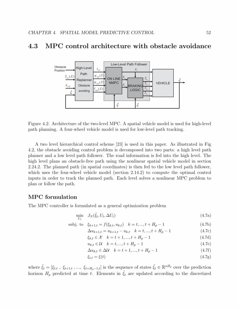
CHAPTER 4. SPATIAL MODEL PREDICTIVE CONTROL 52
4.3 MPC control architecture with obstacle avoidance
refx&
ξ
BRAKING
LOGIC
ON LINE
NMPC VEHICLEξlfb
T,
rfbT
,
lrbT
,
rrbT
,
)(XYreflb
F
rbF
High-Level
Path
Replanner
Obstacle
avoiding
Obstacle
Position
Low-Level Path Follower
)(Xreplψ&
)(XYrepl
refx&
)(Xreplψ
ξ
ξ
fδ
Figure 4.2: Architecture of the two-level MPC. A spatial vehicle model is used for high-levelpath planning. A four-wheel vehicle model is used for low-level path tracking.
A two level hierarchical control scheme [23] is used in this paper. As illustrated in Fig4.2, the obstacle avoiding control problem is decomposed into two parts: a high level pathplanner and a low level path follower. The road information is fed into the high level. Thehigh level plans an obstacle-free path using the nonlinear spatial vehicle model in section2.24.2. The planned path (in spatial coordinates) is then fed to the low level path follower,which uses the four-wheel vehicle model (section 2.14.2) to compute the optimal controlinputs in order to track the planned path. Each level solves a nonlinear MPC problem toplan or follow the path.
MPC formulation
The MPC controller is formulated as a general optimization problem
minUt
JN (ξt, Ut,∆Ut) (4.7a)
subj. to ξk+1,t = f(ξk,t, uk,t) k = t, ..., t+Hp − 1 (4.7b)
∆uk+1,t = uk+1,t − uk,t k = t, ..., t+Hp − 1 (4.7c)
ξk,t ∈ X k = t+ 1, ..., t+Hp − 1 (4.7d)
uk,t ∈ U k = t, ..., t+Hp − 1 (4.7e)
∆uk,t ∈ ∆U k = t+ 1, ..., t+Hp − 1 (4.7f)
ξt,t = ξ(t) (4.7g)
where ξt = [ξt,t , ξt+1,t , ..., ξt+Hp−1,t] is the sequence of states ξt ∈ RnHp over the prediction
horizon Hp predicted at time t. Elements in ξt are updated according to the discretized
CHAPTER 4. SPATIAL MODEL PREDICTIVE CONTROL 53
dynamics of the vehicle model (4.7b). uk,t and ∆uk,t ∈ Rmr is the kth vector of the inputsequence Ut ∈ RmrHp and ∆Ut ∈ Rmr(Hp−1) respectively,
Ut = [uTt,t , uTt+1,t , ..., u
Tt+Hu−1,t , u
Tt+Hu,t , ..., u
Tt+Hp−1,t]
T (4.8a)
∆Ut = [∆uTt+1,t, ...,∆uTt+Hu−1,t,∆u
Tt+Hu,t, ...,∆u
Tt+Hp−1,t]
T (4.8b)
Note the time “t” in this section denotes the generalized time, the independent variablewith respect to which the system states are differentiated. Specifically, in the high level it isthe spatial coordinate “s” while in the low level it is the time t.
The computational complexity of the MPC problem is reduced by two means. One is tohold the last Hp −Hu input vectors in Ut constant and equal to the vector ut+Hu−1,t. Withthis assumption, only the first Hu input vectors constitutes the optimization variables. Theother one is to keep the input vectors constant for every iHu steps in the first Hu inputvectors (i.e., set ut+n·iHu+k,t = ut+n·iHu,t, ∀k = 1, 2...iHu). With this assumption, the numberof optimization variables is further reduced. We refer to Hp as the prediction horizon, Hu asthe control horizon and iHu as the input blocking factor.
At each time step t, the performance index JN(ξt, Ut,∆Ut) is optimized under the con-straints (4.7c)-(4.7f) starting from the state ξt,t = ξ(t) to obtain an optimal control sequence,U∗t = [u∗t,t
T , ..., u∗t+Hp−1,tT ]T . The first of such optimal moves u∗t,t is the control action applied
to the vehicle at time t. At time t+1, a new optimization is solved over a shifted predictionhorizon starting from the new measured state ξt+1,t+1 = ξ(t+1). The time interval betweentime step t+ 1 and time step t is the sampling time Ts.
High level path planner
The High level MPC uses the spatial bicycle vehicle model. Specifically, in equation (4.7b)we use a discretized version of the equation 4.6.
The cost function considers the deviation of the tracking states ηhlk,s = [xk,s , ψk,s, eψk,s, eyk,s ]
T
with respect to the reference ηhlrefk,s = [xk,s , ψk,s, eψk,s, eyk,s ]
T , as well as the input and inputrate.
JN (ξs, Us,∆Us) =
s+Hp,hl−1∑k=s
∥ηhlk,s − ηhlrefk,s∥2Qhl
+
+∥uk,s∥2Rhl+ ∥∆uk,s∥2Shl
(4.9)
Where the reference xrefk,s is a given constant, eψrefk,sand eyrefk,s are zero, ψrefk,s is defined
as ψ′s · xrefk,s . Qhl, Rhl and Shl are weighting matrices with proper dimensions. The index
for general time “t” is replaced by “s” here. The distance interval between step s+ 1 ands is the sampling interval ds.
A spatial horizon allows one to formulate obstacle constraints as simple bounds on ey andinclude them in the state constraints (4.7d). At each prediction step, the vehicle positionalong the lane center is known to be (s + k · ds). According to the position and widthof the obstacle, one can determine the bounds on ey. With one obstacle, there are two
CHAPTER 4. SPATIAL MODEL PREDICTIVE CONTROL 54
disconnected regions of feasible ey, respectively corresponding to passing the obstacle fromleft and right. In this paper, a simple heuristic based on the vehicle position and the size ofeach feasible region is used to determine which side should the vehicle pass through. In thecase of multiple obstacles at the same coordinate “s”, a similar approach can still be used.
The optimal trajectory [x∗(s), ψ∗(s), e∗ψ(s), e∗y(s), t
∗(s)] is computed by simulating thevehicle model with the optimal inputs from the MPC problem and then passed to the lowlevel path follower. Note t∗(s) can be easily retrieved as described in section 2.24.2. In thelow level, this spatial trajectory is transformed back to a time-dependent trajectory [x∗(t),ψ∗(t), ψ∗(t), Y ∗(t), X∗(t)] by coordinate transformation and interpolation.
Low level path follower
The low level MPC uses the four wheel vehicle model from section 4.2. At each time stept, the system dynamics are linearized around the equilibrium trajectory [ξk,t, uk,t], withuk,t = ut,t ∀k = t, ..., t + Hp,ll and ξk+1,t = f 4w
d (ξk,t, uk,t), where f4wd is the discrete version
of the equation ξ(t) = f 4w(ξ(t), u(t)). The details of the linearizing process can be found in[17].
The cost function again consists of the deviation of the tracking states ηllk,t = [xk,t, ψk,t,
ψk,t, Yk,t]T from the reference ηllrefk,t = [xrefk,t , ψrefk,t , ψrefk,t , Yrefk,t ]
T as well as the input and
input rate penalty.
JN (ξt, Ut,∆Ut) =
s+Hp,ll−1∑k=t
∥ηllk,t − ηllrefk,t∥2Qll
+
∥uk,t∥2Rll+ ∥∆uk,t∥2Sll
(4.10)
The inputs vector uk,t = [δf , Fbl , Fbr ]T consists of the steering angle δf , left braking
force Frl and right braking force Fbr . The braking logic in [19] is used to distribute thecorresponding torques at the four wheels.
4.4 Simulation and experimental results
Simulation and experimental tests are conducted to evaluate the proposed controller. TheMPC problem has been implemented as a C-coded s-function where NPSOL [25] is used tosolve the high level optimization. At the low-level, the nonlinear program is solved by usinga sequential quadratic programming approach [18] and the quadratic program is solved usingthe QP solver routine available in [59], which implements the Dantzig-Wolfe’s algorithm.
Simulation setup description
Real-time simulation of the controller is tested on a dSPACE rapid prototyping systemconsisting of a MicroAutoBox and a DS1006 processor board with a DS2211 I/O board.
CHAPTER 4. SPATIAL MODEL PREDICTIVE CONTROL 55
The controller runs on the MicroAutoBox. The first element of the optimal control sequenceis passed to DS1006 board, which simulates the vehicle dynamics using a four wheel vehiclemodel and Pacejka tire model [1], and then feeds the current vehicle state back to thecontroller. The two components communicate through a CAN bus.
Experimental setup description
The experiments have been performed at a test center equipped with icy and snowy handlingtracks. The MPC controller has been tested on a passenger car, with a mass of 2050 Kgand a yaw inertia of 3344 Kg/m2. The controllers were run in a dSPACE Autobox system,equipped with a DS1005 processor board and a DS2210 I/O board.
We used an Oxford Technical Solution (OTS) RT3002 sensing system to measure thevehicle position and orientation in the inertial frame and the vehicle velocities in the vehiclebody frame. The OTS RT3002 is housed in a small package that contains a differential GPSreceiver, Inertial Measurement Unit (IMU) and a DSP. The IMU includes three accelerom-eters and three angular rate sensors. The DSP receives both the measurements from theIMU and the GPS, utilizes a Kalman filter for sensor fusion, and calculates the position,orientation and other states of the vehicle.
The car was equipped with an Active Front Steering (AFS) and Differential Brakingsystem which utilizes an electric drive motor to change the relation between the hand steeringwheel and road wheel angles. This is done independently from the hand wheel position, thusthe front road wheel angle is obtained by summing the driver hand wheel position and theactuator angular movement.
The sensor, the dSPACE Autobox and the actuators communicate through a CAN bus.
Results and discussions
The controller is tested with the following tuning: Tuning HL Hierarchical MPC High-level:Nonlinear MPC (4.7) with model (4.6) and cost (4.9) and with the following parameters.
• ds = 1.5m, Hp,hl = 15, Hu,hl = 12, iHu,hl = 3
• δf ∈ [−10 , 10 ], ∆δf ∈ [−17 , 17 ]× ds
• βr ∈ [−1, 1], ∆βr ∈ [−10, 10]× ds
• Qhl = diag(1, 1, 20, 1), Rhl = diag(50, 50)Shl = diag(0.1, 0.1)
Tuning LL Hierarchical MPC Low-level: Nonlinear MPC (4.7) with model (4.2) and cost (4.10)and with the following parameters
• Ts,ll = 0.05s, Hp,ll = 5, Hu,ll = 3, iHu,ll = 1
• δf ∈ [−10 , 10 ], ∆δf ∈ [−17 , 17 ]× Ts,ll

CHAPTER 4. SPATIAL MODEL PREDICTIVE CONTROL 56
0 50 100 150−10
−5
0
5
10
X(m)
Y(m
)
Planned pathActual pathObstacleCenter line
Figure 4.3: Simulated result: The vehicle entered the maneuver at 50 kph. The green linesare planned paths from the high-level which are updated every 200 ms. The black line is theactual trajectory the vehicle traveled.
• Fb• ∈ [−1500, 0], ∆Fb• ∈ [−1000, 1000]× Ts,ll
• Q = diag(10, 20, 10, 50), R = diag(1, 0.5, 0.5)S = diag(1, 0.1, 0.1)
The simulation and experimental results are summarized in Figures 4.3 to 4.6. In all tests,the road friction coefficient is approximately 0.3. The high level path planner is invokedevery 200ms, and the low level every 50ms.
Since the obstacle constraint is formulated as hard constraints on the states, the highlevel path planner will always plan a tight path passing the obstacle due to the tracking errorand input penalties, see the green line right below the obstacle in figure 4.3 as an example.To avoid this problem, an unsafe zone around the obstacle is added in the tests. The unsafezones are shown in gray in figure 4.4 to 4.6.
Figure 4.3 and 4.4 are the simulation and experimental results of the vehicle avoidingone obstacle on a slippery road. The two tests show consistent performance. Figure 4.5 and4.6 show the experimental results for avoiding two obstacles with different distances betweenthem. In both cases the vehicle was able to avoid both obstacles and get back to the lanecenter afterwards. In figure 4.6 when the distance between the two obstacles was large, thevehicle was already trying to get back to the lane center before the second obstacle cameinto the planning horizon.
Figure 4.7 compares the controller’s performance with a previously proposed controllerin [23], which uses a time-dependent point mass model at the high level. The blue dots inthe figures are the reference for the low level at each sampling time. We observe that the useof a nonlinear bicycle model at the high level greatly improves the tracking performance.

CHAPTER 4. SPATIAL MODEL PREDICTIVE CONTROL 57
0 50 100 150−10
−5
0
5
10
X[m]
Planned pathActual pathObstacleUnsafe zoneCenter line
Figure 4.4: Experimental result: The vehicle entered the maneuver at 50 kph. Friction coef-ficient of the ground was approximately 0.3. The vehicle avoided the obstacle and continuedto track the lane center. The green lines are planned paths from the high-level which wereupdated every 200 ms. The black line is the actual trajectory the vehicle traveled.
0 50 100 150 200−10
−5
0
5
10
X[m]
Y[m
]
Planned pathActual pathObstacleUnsafe zoneCenter line
Figure 4.5: Experimental result: The vehicle entered the maneuver at 50 kph. Frictioncoefficient of the ground was approximately 0.3. The vehicle avoided the two obstacles andcontinued to track the lane center.

CHAPTER 4. SPATIAL MODEL PREDICTIVE CONTROL 58
0 50 100 150 200 250 300−10
−5
0
5
10
X[m]
Y[m
]
Planned pathActual pathObstacleUnsafe zoneCenter line
Figure 4.6: Experimental result: The vehicle entered the maneuver at 50 kph. Frictioncoefficient of the ground was approximately 0.3. The vehicle avoided the first obstacle andcontinued to track the lane center until the second obstacle came into sight. It then turnedleft to avoid the second obstacle.
The use of a spatial model at the high level makes the construction of obstacle constraintsstraight forward as described in section 3.1 4.3. On the other hand, the hard constraintformulation for obstacle is not trivial for general shaped obstacles in MPC formulation withtime-dependent models. Potential field approaches are a commonly used solution approach.Of course, it is possible to find indicating functions whose level sets can be used to formthe obstacle constraints. This is usually not straight forward, especially if one wants theindicating function to have nice properties, such as differentiability, in order to speed up theoptimization problem.
4.5 Concluding Remarks
In this chapter, a hierarchical design of a spatial MPC controller is presented for the obsta-cle avoiding and lane keeping problem of a ground vehicle on a slippery road. The controlproblem is decomposed into a high level path planner and a low level path follower. Thehigh level uses a simplified spatial model while the low level uses a higher fidelity model. Ex-perimental results show the controller is real-time implementable and able to avoid multipleobstacles at high speeds on slippery road.
Compared to the point mass model hierarchical MPC in the previous chapter, the trackingof the vehicle trajectory to the planed trajectory is greatly improved by the use of the spatialbicycle model. However, the high level planned path will never be tracked perfectly dueto the model mismatch, state estimation error and external disturbances. Thus collisionavoidance is not guaranteed even when the high level planned path is obstacle free. The

CHAPTER 4. SPATIAL MODEL PREDICTIVE CONTROL 59
0 20 40 60 80 100 120
−2
0
2
X[m]
Y[m
]
Low lvl referenceActual pathObstacle
(a) Simulation result of the controller in [23]. A time-dependentpoint mass model is used for the high level. The vehicle turns earlybecause the high level uses a potential field approach for obstacleavoidance.
0 20 40 60 80 100 120−3
−2
−1
0
1
2
3
X[m]
Y[m
]
Low lvl referenceActual pathObstacle
(b) Simulation result of the new controller. A spatial-dependentbicycle model is used for the high level.
Figure 4.7: Simulation result comparison with the controller proposed in [23]. In both casesthe high levels replan every 200ms. The same low level path follower is used, which uses anonlinear four wheel model and runs every 50ms.

CHAPTER 4. SPATIAL MODEL PREDICTIVE CONTROL 60
next chapter approaches this issue by proposing a robust NMPC framework which enforcesrobust constraint satisfaction under the presence of uncertainties.

61
Chapter 5
Robust Nonlinear Model PredictiveControl
5.1 Introduction
Previous chapters have addressed the problem of autonomous and semiautonomous obstacleavoidance and lane keeping, by an approach of hierarchical MPC scheme. Successful imple-mentations of such MPC scheme on autonomous vehicle driving ar high speeds on slipperyicy-snow track have been reported in [23, 24, 27]. However, robust constraint satisfactionis not guaranteed. Because uncertainties from a variety of sources might still prevent thevehicle from following the desired path and satisfying the safety constraints. Such uncertain-ties include measurement errors, friction coefficient estimation, driver behavior and modelmismatch.
This chapter presents a systematic way of enforcing robustness under the presence ofuncertainties during the MPC design stage. A robust nonlinear MPC framework [36, 43,44, 55, 65, 2, 45, 63] is used in this chapter. In particular we follow the “Tube” approachpresented in [63] for nonlinear system where the inputs enter linearly in the state updateequations. The basic idea is to use a control law of the form u = u+K(ξ − ξ) where u andξ are the nominal control input and system states trajectories. For a given linear controllerK, a robust invariant set is computed for the error system. The invariant is used to boundthe maximum deviation of the actual states from the nominal states under the linear controlaction K. A nominal MPC optimizes u and ξ with tightened state and input constraints.The tightening is computed as a function of the bounds derived from the robust invariantset.
In the first part of the chapter we propose a force-input nonlinear bicycle vehicle model.The model captures the main nonlinear vehicle dynamics and the input forces enter linearlythe system equations. In the second part we show how to compute the robust invariantfor the nonlinear system controlled in closed-loop by a linear state-feedback controller. Theinvariant set is computed utilizing the lipschitz constant of the nonlinear systems. In the
CHAPTER 5. ROBUST NONLINEAR MODEL PREDICTIVE CONTROL 62
third part we use the robust invariant set computed off-line to tighten the state and inputconstraints for a nominal nonlinear MPC problem which computes obstacle-free trajectoriesand corresponding input sequences. Simulations and experiments in different scenarios showthe effectiveness of the proposed approach. In particular, in the last part of the chapter,nominal MPC is compared with the proposed approach in terms of performance and constrainsatisfaction.
This chapter is structured as follows. In section 5.2 the definitions of invariant sets arepresented, the Robust MPC framework is outlined and the method used for computing therobust invariant set is introduced. In section 5.3 the force-input nonlinear vehicle modelwith additive uncertainty is developed. Section 5.4 details the robust invariant set computa-tion. Section 5.5 presents the safety constraints and section 5.6 formulates the Robust MPCproblem. Finally, in section 5.7 and 5.8 we present the simulation and experimental resultsshowing the behavior of the proposed controller.
5.2 Invariant set and robust MPC
Background on set invariance theory
In this section several definitions are provided that will be important in developing theRobust MPC later in this chapter.
We denote by fa the constrained, discrete time linear autonomous system perturbed bya bounded, additive disturbance
ξk+1 = fa(ξk) + wk, (5.1)
where ξk and wk denote the state and the disturbance vectors. System (5.1) is subject tothe constraints
ξk ∈ Ξ ⊆ Rn, wk ∈ W ⊆ Rd, (5.2)
where Ξ and W are polyhedra that contain the origin in their interiors.
Definition 1 (Reachable Set for autonomous systems) Consider the autonomous system(5.1)-(5.2). The one-step robust reachable set from a given set of states S is
Reachfa(S,W)= ξ ∈ Rn|
∃ ξ0 ∈ S, ∃ w ∈ W : ξ = fa(ξ0, w).(5.3)
Similarly, for systems with inputs
ξk+1 = f(ξk, uk) + wk, (5.4)
subject to the constraints
ξk ∈ Ξ, uk ∈ U ⊆ Rm, wk ∈ W , (5.5)
we use the following definition of the one-step robust reachable set.

CHAPTER 5. ROBUST NONLINEAR MODEL PREDICTIVE CONTROL 63
Definition 2 (Reachable set for systems with external inputs) Consider the system (5.4)-(5.5). The one-step robust reachable set from a given set of states S is
Reachf (S,W)= ξ ∈ Rn|
∃ ξ0 ∈ S, ∃ u ∈ U , ∃ w ∈ W : ξ = f(ξ0, u, w).(5.6)
All states contained in S are mapped into the reachable set Reachfa under the map fafor all disturbances w ∈ W , and under the map f for all inputs u ∈ U and all disturbancesw ∈ W . We will next define robust invariant sets.
Definition 3 (Robust Positively Invariant Set) A set Z ⊆ Ξ is said to be a robust positivelyinvariant set for the autonomous system (5.1) subject to the constraints in (5.2), if
ξ0 ∈ Z ⇒ ξk ∈ Z, ∀wk ∈ W , ∀k ∈ N+. (5.7)
Definition 4 (Maximal Robust Positively Invariant Set) The set Z∞ ⊆ Ξ is the maximalrobust invariant set for the autonomous system (5.1) subject to the constraints in (5.2), ifZ∞ is a robust positively invariant set and Z∞ contains all robust positively invariant setscontained in Ξ that contain the origin.
Two set operations will be used in this article: the Pontryagin difference and the Minkowskisum. The Pontryagin difference of two polytopes P and Q is a polytope
P ⊖Q := x ∈ Rn : x+ q ∈ P , ∀q ∈ Q, (5.8)
and the Minkowski sum of two polytopes P and Q is a polytope
P ⊕Q := x+ q ∈ Rn : x ∈ P , q ∈ Q. (5.9)
The Multi-Parametric Toolbox (MPT) [35] can be used for the set computations.
Background on robust MPC
In this section we outline the framework used to develop the robust model predictive con-troller in section 5.6. We follow a notation similar to [43]. Consider the system:
ξk+1 = Aξk + g(ξk) +Buk + wk. (5.10a)
s.t. ξk ∈ Ξ (5.10b)
uk ∈ U (5.10c)
Where g(·) : Rn 7→ Rn is a nonlinear Lipschitz function and wk ∈ W ⊂ Rn is an additivedisturbance. We assume that the matrix pair (A,B) is controllable.
The control problem is divided into two parts. First a feedforward control input iscomputed for the system (5.10). System (5.10) with the computed feedforward input and

CHAPTER 5. ROBUST NONLINEAR MODEL PREDICTIVE CONTROL 64
a zero disturbance sequence will be called the “nominal system”. Then, we design a statefeedback controller which acts on the error between the actual state of system (5.10) andthe predicted state of the nominal system. Next we formalize the aforementioned ideas.
We denote the N -step control sequence and the N -step disturbance sequence for system(5.10) as u = u0, u1, ..., uN−1 and w = w0, w1, ..., wN−1, respectively. Let Φ(k, x,u,w)denote the solution of (5.10) at time k controlled by u when x0 = x. Furthermore, letΦ(k, x, u) denote the solution of the nominal system:
ξk+i+1 = Aξk+i + g(ξk+i) + Buk+i, ∀i = 0, 1, ..., N − 1. (5.11)
Let ek = ξk− ξk be the error between the states of system (5.10) and the nominal system.Let the input uk to system (5.10) be:
uk = uk + u(ek), (5.12)
where u(ek) : Rn 7→ Rm. We define the error dynamics as:
ek+1 = Aek +Bu(ek) + (g(ξk)− g(ξk)) + wk. (5.13)
The authors of [43] proved the following result.
Proposition 1 Suppose that Z is a Robust Positively Invariant Set of the error system(5.13) with control law u(·). If ξk ∈ ξk ⊕ Z, then ξk+i ∈ ξk+i ⊕ Z for all i > 0 and alladmissible disturbance sequences wk+i ∈ W.
Proposition 1 states that if the state ξ0 of system (5.10) starts close to the nominalstate ξ0, the control law (5.12) will keep the state trajectory Φ(k, x,u,w) within the robustpositively invariant set Z centrex at the predicted nominal states Φ(k, x, u) for all admissibledisturbance sequence w:
ξ0 ∈ ξ0 ⊕ Z ⇒ ξk ∈ ξk ⊕ Z ∀wk ∈ W , ∀k ≥ 0. (5.14)
Proposition 1 also suggests that if a feasible solution can always be found for the nominalsystem (5.11) subject to the tightened constraints
Ξ = Ξ⊖Z, U = U ⊖ u(Z), (5.15)
then the control law (5.12) will ensure constraint satisfaction for the controlled uncertainsystem (5.10) [2].
Remark 5 For general nonlinear systems, the controller and invariant set pair (u(·), Z)is usually hard to find. In the following section we will propose an algorithm for computing(u(·), Z) for system in the form of (5.10), whose dynamics consist of a linear term Aξ+Buand a “small” nonlinear term g(ξ).

CHAPTER 5. ROBUST NONLINEAR MODEL PREDICTIVE CONTROL 65
Computation of the robust invariant set
In [63], the authors present a test criterion to determine if a given linear feedback controller,u = Ke, and an ellipsoidal set of the system states form a valid controller-invariant set pair.In this section we use a similar approach. In particular we use the Lipschitz constant of thenonlinear term to compute a robust invariant set.
The main idea is to bound the nonlinear term (g(ξ)−g(ξ)) in (5.13) by using the Lipschitzconstant of g(·), and treat it as part of the disturbance. We use the 2-norm over Rn. Thenonlinear function g(ξ) is Lipschitz in the set Ξ with respect to ξ if ∃L > 0 such that
∥g(ξ1)− g(ξ2)∥2 ≤ L∥ξ1 − ξ2∥2, ∀ξ1, ξ2 ∈ Ξ. (5.16)
The smallest constant L satisfying (5.16) is called the Lipschitz constant.Let L(Ξ) be the Lipschitz constant of g(·) over Ξ. From (5.16) we obtain
∀ξ, ξ ∈ Ξ and e = (ξ − ξ) ∈ E , ∥g(ξ)− g(ξ)∥∞ ≤ L(Ξ)maxe∈E∥e∥2, (5.17)
where E is a subset of Ξ containing 0. The inequality in (5.17) defines a box B(E):
B(E) = x ∈ Rn|∥x∥∞ ≤ L(Ξ)maxe∈E∥e∥2 (5.18)
B(E) is used to bound the term (g(ξk)− g(ξk)) in (5.13). Equation (5.13) is then written as:
ek+1 = Aek +Bu(ek) + wk, (5.19)
where wk ∈ W =W ⊕B(E).
Proposition 2 For ξ, ξ ∈ Ξ, If Z is a robust positively invariant set for system (5.19) witha control law u(·), then Z is a robust positively invariant set for system (5.13) with the samecontrol law u(·).
Proposition 2 is true because all possible values of (g(ξ)−g(ξ)) in (5.13) lies inside B(E).Since we assumed the matrix pair (A,B) to be controllable, there exists a stabilizing
linear feedback gain K such that (A+BK) is Hurwitz. Algorithm 1 is used to compute theminimal robust positively invariant set Z associated with the gain K.
If Algorithm 1 terminates in finitely many iterations it, then Z = Ωit is the minimalpositively invariant set for the uncertain system (5.19) [54]. The choice of K will determinethe size of Z, and also the size of KZ. Later in this chapter we will show that KZ is usedto tighten the input constraints for ensuring robust constraint satisfaction. A larger K willresult in a smaller Z, in general, but may lead to larger KZ and thus smaller input actions.
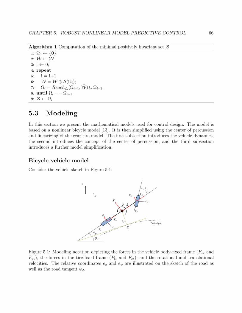
CHAPTER 5. ROBUST NONLINEAR MODEL PREDICTIVE CONTROL 66
Algorithm 1 Computation of the minimal positively invariant set Z1: Ω0 ← 02: W ← W3: i ← 0;4: repeat5: i = i+16: W =W ⊕B(Ωi);7: Ωi = Reachfa(Ωi−1, W) ∪ Ωi−1.8: until Ωi == Ωi−1
9: Z ← Ωi
5.3 Modeling
In this section we present the mathematical models used for control design. The model isbased on a nonlinear bicycle model [13]. It is then simplified using the center of percussionand linearizing of the rear tire model. The first subsection introduces the vehicle dynamics,the second introduces the concept of the center of percussion, and the third subsectionintroduces a further model simplification.
Bicycle vehicle model
Consider the vehicle sketch in Figure 5.1.
y
x
yfF
cfF
xfF
lfF
ye
yrF
xrF
crFlrF
e
d
S
Desired path
Y
X
Figure 5.1: Modeling notation depicting the forces in the vehicle body-fixed frame (Fx⋆ andFy⋆), the forces in the tire-fixed frame (Fl⋆ and Fc⋆), and the rotational and translationalvelocities. The relative coordinates ey and eψ are illustrated on the sketch of the road aswell as the road tangent ψd.
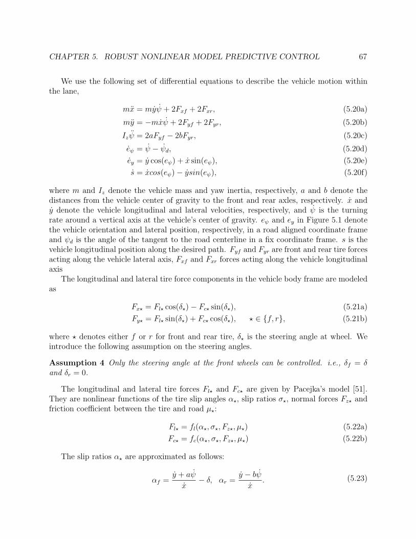
CHAPTER 5. ROBUST NONLINEAR MODEL PREDICTIVE CONTROL 67
We use the following set of differential equations to describe the vehicle motion withinthe lane,
mx = myψ + 2Fxf + 2Fxr, (5.20a)
my = −mxψ + 2Fyf + 2Fyr, (5.20b)
Izψ = 2aFyf − 2bFyr, (5.20c)
eψ = ψ − ψd, (5.20d)
ey = y cos(eψ) + x sin(eψ), (5.20e)
s = xcos(eψ)− ysin(eψ), (5.20f)
where m and Iz denote the vehicle mass and yaw inertia, respectively, a and b denote thedistances from the vehicle center of gravity to the front and rear axles, respectively. x andy denote the vehicle longitudinal and lateral velocities, respectively, and ψ is the turningrate around a vertical axis at the vehicle’s center of gravity. eψ and ey in Figure 5.1 denotethe vehicle orientation and lateral position, respectively, in a road aligned coordinate frameand ψd is the angle of the tangent to the road centerline in a fix coordinate frame. s is thevehicle longitudinal position along the desired path. Fyf and Fyr are front and rear tire forcesacting along the vehicle lateral axis, Fxf and Fxr forces acting along the vehicle longitudinalaxis
The longitudinal and lateral tire force components in the vehicle body frame are modeledas
Fx⋆ = Fl⋆ cos(δ⋆)− Fc⋆ sin(δ⋆), (5.21a)
Fy⋆ = Fl⋆ sin(δ⋆) + Fc⋆ cos(δ⋆), ⋆ ∈ f, r, (5.21b)
where ⋆ denotes either f or r for front and rear tire, δ⋆ is the steering angle at wheel. Weintroduce the following assumption on the steering angles.
Assumption 4 Only the steering angle at the front wheels can be controlled. i.e., δf = δand δr = 0.
The longitudinal and lateral tire forces Fl⋆ and Fc⋆ are given by Pacejka’s model [51].They are nonlinear functions of the tire slip angles α⋆, slip ratios σ⋆, normal forces Fz⋆ andfriction coefficient between the tire and road µ⋆:
Fl⋆ = fl(α⋆, σ⋆, Fz⋆, µ⋆) (5.22a)
Fc⋆ = fc(α⋆, σ⋆, Fz⋆, µ⋆) (5.22b)
The slip ratios α⋆ are approximated as follows:
αf =y + aψ
x− δ, αr =
y − bψx
. (5.23)
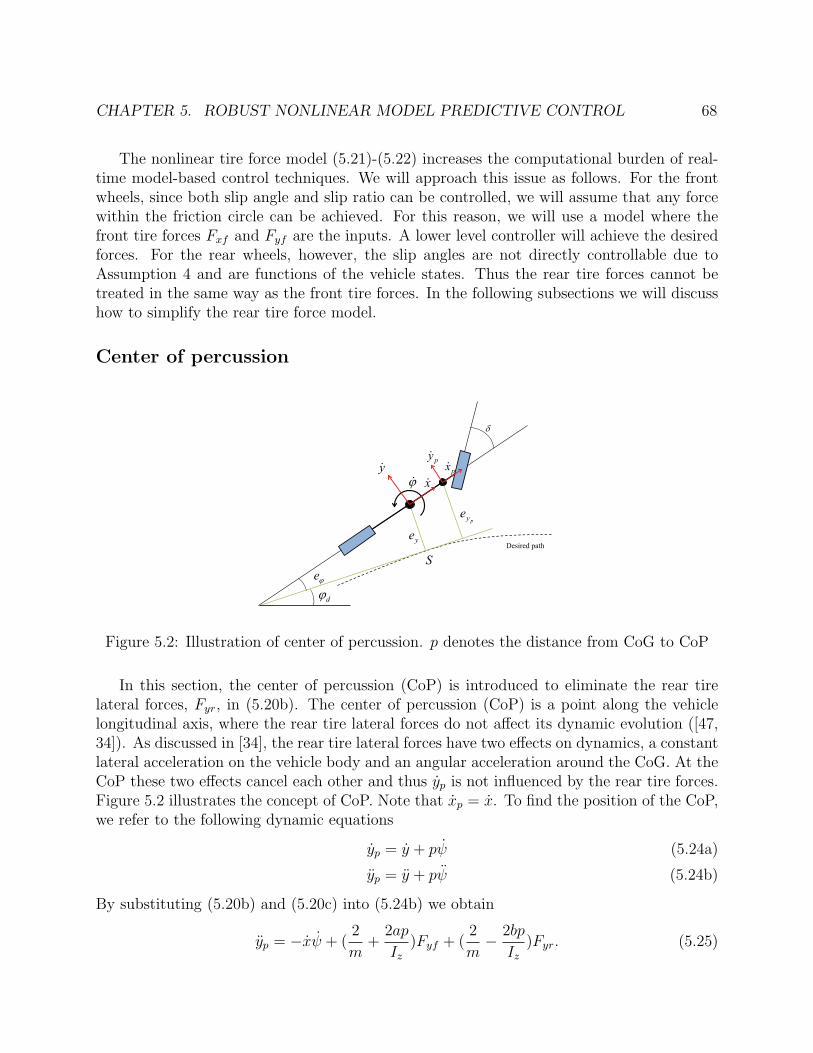
CHAPTER 5. ROBUST NONLINEAR MODEL PREDICTIVE CONTROL 68
The nonlinear tire force model (5.21)-(5.22) increases the computational burden of real-time model-based control techniques. We will approach this issue as follows. For the frontwheels, since both slip angle and slip ratio can be controlled, we will assume that any forcewithin the friction circle can be achieved. For this reason, we will use a model where thefront tire forces Fxf and Fyf are the inputs. A lower level controller will achieve the desiredforces. For the rear wheels, however, the slip angles are not directly controllable due toAssumption 4 and are functions of the vehicle states. Thus the rear tire forces cannot betreated in the same way as the front tire forces. In the following subsections we will discusshow to simplify the rear tire force model.
Center of percussion
y
x
ye
e
d
S
Desired path
py
px
pye
Figure 5.2: Illustration of center of percussion. p denotes the distance from CoG to CoP
In this section, the center of percussion (CoP) is introduced to eliminate the rear tirelateral forces, Fyr, in (5.20b). The center of percussion (CoP) is a point along the vehiclelongitudinal axis, where the rear tire lateral forces do not affect its dynamic evolution ([47,34]). As discussed in [34], the rear tire lateral forces have two effects on dynamics, a constantlateral acceleration on the vehicle body and an angular acceleration around the CoG. At theCoP these two effects cancel each other and thus yp is not influenced by the rear tire forces.Figure 5.2 illustrates the concept of CoP. Note that xp = x. To find the position of the CoP,we refer to the following dynamic equations
yp = y + pψ (5.24a)
yp = y + pψ (5.24b)
By substituting (5.20b) and (5.20c) into (5.24b) we obtain
yp = −xψ + (2
m+
2ap
Iz)Fyf + (
2
m− 2bp
Iz)Fyr. (5.25)

CHAPTER 5. ROBUST NONLINEAR MODEL PREDICTIVE CONTROL 69
When p = Izmb
, the Fyr term in (5.25) vanishes.
Simplifying rear tire forces
The use of the CoP eliminates the rear tire force in yp. However, the rear tire forces are stillpresent in the longitudinal and yaw dynamics xp and ψ. We will use a linearized tire modelfor these terms.
−10 −5 0 5
−2000
−1500
−1000
−500
0
500
1000
1500
2000
α [deg]
Fc[N
]
Pacejka at βr ∈ [−0.5 0]Linear ApproximationBnd. of Linear Region
Figure 5.3: Lateral tire force. µ is 0.5 in Pacejka tire model. When βr varies moderately, Fcbehaves similar within the linear region.
Let βr denote the braking/throttle ratio of rear tire (Flr = βrµFzr), with βr=1 corre-sponding to max throttle and -1 max braking. In moderate braking, the resultant lateraltire force Fc as a function of slip angle α has small sensitivity with respect to βr, as shownin Fig 5.3. Thus a constant linear gain can be used over β ∈ [−0.5 0] and over β ∈ [0 0.5].The remaining rear tire forces in (5.20a) and (5.20c) are modeled as:
Flr = βrµFzr (5.26a)
Fcr = Crαr (5.26b)
Remark 6 The same linearization could be applied to the Fyr term in (5.20b). We decidedto use CoP to eliminate it (Section 5.3) to reduce the error introduced by the linearization.

CHAPTER 5. ROBUST NONLINEAR MODEL PREDICTIVE CONTROL 70
Force-input nonlinear bicycle model
In summary, the nominal vehicle model (5.20) used for control design is rewritten as:
yp =2(a+ b)µFzfβxf
mb− ψxp, (5.27a)
xp =2µFzfβxf
m+
2µFzrβrm
+ ψyp − ψ2p, (5.27b)
ψ =2aµFzfβyf
Iz− 2bCryp
Izxp+
2bCr(b+ p)ψ
Izxp, (5.27c)
eψ = ψ − ψd, (5.27d)
ey = yp + xpeψ, (5.27e)
s = xp (5.27f)
where the state is ξ = [yp, xp, ψ, eψ, ey, s]T ∈ R6×1, and the input is u = [βxf , βyf , βr]
T ∈ R3.βxf and βyf are the normalized longitudinal and lateral tire forces on the front wheels.
The following assumptions are used in (5.27):
Assumption 5 The vehicle orientation error with respect to the road orientation, eψ, issmall and thus sin(eψ) ≃ eψ, cos(eψ) ≃ 1. The vehicle side slip angle is assumed to besmall, i.e. y ≪ x and yp ≪ xp.
Assumption 6 The normal forces Fz⋆ are assumed constant and determined by the vehicle’ssteady state weight distribution when no acceleration is applied
Assumption 7 The signal ψd is assumed to be known and at every time instant an estimateof ψd is available over a finite time horizon. See [4] for an overview of sensing technologiesthat can be used to obtain this signal.
5.4 Invariant set computation
The objective of the robust MPC is to safely navigate the vehicle to avoid obstacles andstay on the road, in the presence of uncertainties. Uncertainties include measurement er-rors, friction coefficient estimation, driver behavior and model mismatch. In this sectionwe derive the robust control law defined in (5.12) for the system (5.28), and provide thedetails of computing the robust positively invariant set used to guarantee robust constraintsatisfactions.
Model reformulation
Equation (5.27) can be written in a similar form of (5.10):
ξ = Aξ + g(ξ) +Bu+G+ w, (5.28)

CHAPTER 5. ROBUST NONLINEAR MODEL PREDICTIVE CONTROL 71
where all nonlinear terms are collected in g(·) : Rn 7→ Rn. The matrices in (5.28) are
A =
0 0 −¯xp 0 00 0 0 0 0
−2bCr
I ¯xp0 2bCr(p+b)
I ¯xp0 0
0 0 1 0 01 0 0 ¯xp 00 1 0 0 0
,
g(ξ) =
−∆xpψψyp − ψ2p
2bCr(yp∆xp−(p+b)ψ∆xp)
Iz ¯xp(¯xp+∆xp)
0∆xpeψ
0
, (5.29a)
B =
02µFzf
m+
2aµFzf
mb0
2µFzf
m0 2µFzr
m
02aµFzf
Iz0
0 0 00 0 00 0 0
, G =
000
−ψd00
, (5.29b)
Note xp is rewritten as xp = ¯xp+∆xp. The signal w represents an additive disturbance. Wefollow the approach described in section 5.2 to compute the minimal positively invariant setZ (also called the tube). The algorithm requires an error model, a linear feedback gain and adescription of potential disturbance bounds. We use the model (5.28) and (5.29) to computethe error model and the lipschitz constant as described in section 5.2. The selection of thegain is described in section 5.4, and the computation of the disturbance bounds in section5.4.
Choice of linear stabilising gain
We choose the stabilising state feedback gain K for the error system as the infinite horizonLQR solution K∞
LQR for system (A,B). Therefore the controller (5.12) becomes:
uk = uk +K∞LQR(ξk − ξk). (5.30)
The controller K is used in the computation of the robust invariant set Z. Z is computedoff-line using Algorithm 1 and a sampled version of (5.28) with a sampling time of 50ms.Specifically, for our system described in (5.28), the linear part of the dynamics are separatedinto two parts: the longitudinal part includes the states [xp, s] and inputs [βxf , βr]; andthe lateral part includes the states [yp, ψ, eψ, ey] and the input βyf . The corresponding
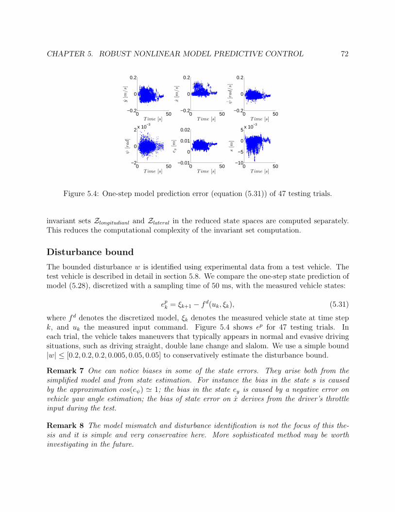
CHAPTER 5. ROBUST NONLINEAR MODEL PREDICTIVE CONTROL 72
0 50−0.2
0
0.2
T ime [s]y[m
/s]
0 50−0.2
0
0.2
T ime [s]
x[m
/s]
0 50−0.2
0
0.2
T ime [s]
ψ[rad/s]
0 50−2
0
2x 10
−3
T ime [s]
ψ[rad]
0 50−0.01
0
0.01
0.02
T ime [s]e y
[m]
0 50−10
−5
0
5x 10
−3
T ime [s]
s[m
]
Figure 5.4: One-step model prediction error (equation (5.31)) of 47 testing trials.
invariant sets Zlongitudianl and Zlateral in the reduced state spaces are computed separately.This reduces the computational complexity of the invariant set computation.
Disturbance bound
The bounded disturbance w is identified using experimental data from a test vehicle. Thetest vehicle is described in detail in section 5.8. We compare the one-step state prediction ofmodel (5.28), discretized with a sampling time of 50 ms, with the measured vehicle states:
epk = ξk+1 − fd(uk, ξk), (5.31)
where fd denotes the discretized model, ξk denotes the measured vehicle state at time stepk, and uk the measured input command. Figure 5.4 shows ep for 47 testing trials. Ineach trial, the vehicle takes maneuvers that typically appears in normal and evasive drivingsituations, such as driving straight, double lane change and slalom. We use a simple bound|w| ≤ [0.2, 0.2, 0.2, 0.005, 0.05, 0.05] to conservatively estimate the disturbance bound.
Remark 7 One can notice biases in some of the state errors. They arise both from thesimplified model and from state estimation. For instance the bias in the state s is causedby the approximation cos(eψ) ≃ 1; the bias in the state ey is caused by a negative error onvehicle yaw angle estimation; the bias of state error on x derives from the driver’s throttleinput during the test.
Remark 8 The model mismatch and disturbance identification is not the focus of this the-sis and it is simple and very conservative here. More sophisticated method may be worthinvestigating in the future.

CHAPTER 5. ROBUST NONLINEAR MODEL PREDICTIVE CONTROL 73
5.5 Safety constraints
The main objective of the safety system proposed in this chapter is to keep the vehicle onthe road while avoiding obstacles. In this section, we detail the constraints imposed on thevehicle states and inputs to guarantees safe maneuvers.
Road boundary constraint: we constrain the CoG of the vehicle and shrink the roadbounds to take the vehicle width into account. The road boundary constraints are writtenas
eymin≤ ey ≤ eymax , (5.32)
where eyminand eymax are obtained from the tightened state constraint Ξ.
Obstacle avoiding constraint: consider ellipsoidal obstacles in the form ( s−sobsaobs
)2+( ey−yobsbobs
)2 ≤1. The obstacle avoiding constraints are written as
(|s− sobs| − sZ
aobs)2 + (
|ey − yobs| − yZbobs
)2 ≥ 1, (5.33)
where sZ and yZ are the projection of the invariant set onto s and ey axes.Slip angle constraint: we constraint the vehicle to operates in a space where a non-skilled
driver can easily handle the vehicle. In particular, we constrain the tire slip angles to belongto the linear region of the tire forces.
αmin ≤ α⋆ ≤ αmax. (5.34)
The constraints (5.32)-(5.34) are compactly written as,
h(ξ, u, w) ≤ 0, (5.35)
where 0 is the zero vector with appropriate dimension.
5.6 Robust predictive control design
In this section we formulate the lane keeping and obstacle avoiding problem as a ModelPredictive Control Problem (MPC). At each sampling time instant an optimal input sequenceis computed by solving a constrained finite time optimal control problem. The computedoptimal control input sequence as well as the corresponding predicted vehicle state trajectoryare stored as the nominal input and state trajectories, ξ and u. At the next time stepthe optimal control problem is solved staring from new state measurements. An algorithmcomputes the augmented input u = u+Ke at sampling time. The MPC and the computationof u can be executed at different sampling times.
We discretize the system (5.28) with a fixed sampling time Ts to obtain,
xk+1 = fn(xk, uk), (5.36)
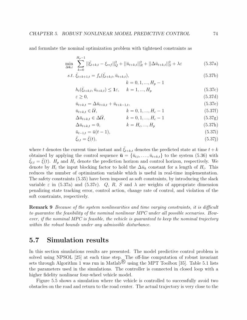
CHAPTER 5. ROBUST NONLINEAR MODEL PREDICTIVE CONTROL 74
and formulate the nominal optimization problem with tightened constraints as
min∆u,ε
Hp−1∑k=0
||ξt+k,t − ξref ||2Q + ||ut+k,t||2R + ||∆ut+k,t||2S + λε (5.37a)
s.t. ξt+k+1,t = fn(ξt+k,t, ut+k,t), (5.37b)
k = 0, 1, ..., Hp − 1
ht(ξt+k,t, ut+k,t) ≤ 1ε, k = 1, ..., Hp (5.37c)
ε ≥ 0, (5.37d)
ut+k,t = ∆ut+k,t + ut+k−1,t, (5.37e)
ut+k,t ∈ U , k = 0, 1, ..., Hc − 1 (5.37f)
∆ut+k,t ∈ ∆U , k = 0, 1, ..., Hc − 1 (5.37g)
∆ut+k,t = 0, k = Hc, ..., Hp (5.37h)
ut−1,t = u(t− 1), (5.37i)
ξt,t = ξ(t), (5.37j)
where t denotes the current time instant and ξt+k,t denotes the predicted state at time t+ kobtained by applying the control sequence u = ut,t, . . . , ut+k,t to the system (5.36) withξt,t = ξ(t). Hp and Hc denote the prediction horizon and control horizon, respectively. Wedenote by Hi the input blocking factor to hold the ∆uk constant for a length of Hi. Thisreduces the number of optimization variable which is useful in real-time implementation.The safety constraints (5.35) have been imposed as soft constraints, by introducing the slackvariable ε in (5.37a) and (5.37c). Q, R, S and λ are weights of appropriate dimensionpenalizing state tracking error, control action, change rate of control, and violation of thesoft constraints, respectively.
Remark 9 Because of the system nonlinearities and time varying constraints, it is difficultto guarantee the feasibility of the nominal nonlinear MPC under all possible scenarios. How-ever, if the nominal MPC is feasible, the vehicle is guaranteed to keep the nominal trajectorywithin the robust bounds under any admissible disturbance.
5.7 Simulation results
In this section simulations results are presented. The model predictive control problem issolved using NPSOL [25] at each time step. The off-line computation of robust invariantsets through Algorithm 1 was run in Matlab R⃝ using the MPT Toolbox [35]. Table 5.1 liststhe parameters used in the simulations. The controller is connected in closed loop with ahigher fidelity nonlinear four-wheel vehicle model.
Figure 5.5 shows a simulation where the vehicle is controlled to successfully avoid twoobstacles on the road and return to the road center. The actual trajectory is very close to the
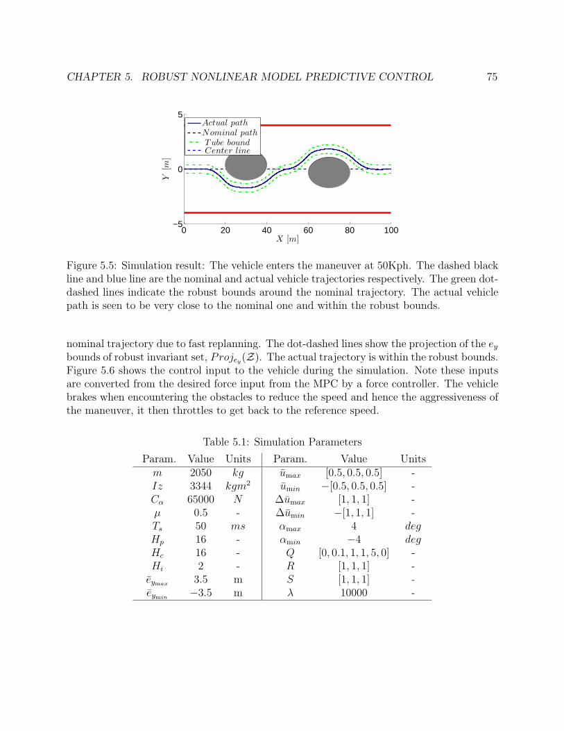
CHAPTER 5. ROBUST NONLINEAR MODEL PREDICTIVE CONTROL 75
0 20 40 60 80 100−5
0
5
X [m]
Y[m
]
Actual path
Nominal path
Tube boundCenter line
Figure 5.5: Simulation result: The vehicle enters the maneuver at 50Kph. The dashed blackline and blue line are the nominal and actual vehicle trajectories respectively. The green dot-dashed lines indicate the robust bounds around the nominal trajectory. The actual vehiclepath is seen to be very close to the nominal one and within the robust bounds.
nominal trajectory due to fast replanning. The dot-dashed lines show the projection of the eybounds of robust invariant set, Projey(Z). The actual trajectory is within the robust bounds.Figure 5.6 shows the control input to the vehicle during the simulation. Note these inputsare converted from the desired force input from the MPC by a force controller. The vehiclebrakes when encountering the obstacles to reduce the speed and hence the aggressiveness ofthe maneuver, it then throttles to get back to the reference speed.
Table 5.1: Simulation Parameters
Param. Value Units Param. Value Unitsm 2050 kg umax [0.5, 0.5, 0.5] -Iz 3344 kgm2 umin −[0.5, 0.5, 0.5] -Cα 65000 N ∆umax [1, 1, 1] -µ 0.5 - ∆umin −[1, 1, 1] -Ts 50 ms αmax 4 degHp 16 - αmin −4 degHc 16 - Q [0, 0.1, 1, 1, 5, 0] -Hi 2 - R [1, 1, 1] -eymax 3.5 m S [1, 1, 1] -eymin
−3.5 m λ 10000 -

CHAPTER 5. ROBUST NONLINEAR MODEL PREDICTIVE CONTROL 76
0 20 40 60 80 100−5
0
5
δ[deg]
0 20 40 60 80 100−0.5
0
0.5βf
0 20 40 60 80 100−0.4−0.2
00.20.4
βr
X [m]
Figure 5.6: Simulation result: Control inputs during the simulation in figure 5.5. βf isthe braking/throttle ratio for the front wheels and βr for the rear wheels. We enable bothbraking and throttle on the wheels in simulation.
Robustness in the presence of disturbance
In this section we show the effectiveness of the controller under large disturbances. Theapproach in this chapter does not use information on the disturbance distribution. It onlyneeds the knowledge of the bounded support in order to enforce robust constraint satisfac-tion for all admissible disturbances. In this section we use a random disturbance with auniform distribution over the bound |w|max = [0.2, 0.2, 0.2, 0.005, 0.05, 0.05]T and add it inthe simulation model at each sampling time. The result is compared to a nominal MPC withthe same parameters but without robustness guarantees, i.e. u = u instead of u = u +Ke.50 trials are run for each controller with random realizations of disturbances. Figure 5.7shows the performance of the nominal MPC. The trajectories are scattered over a large areaand four trials fail to avoid the obstacle. In Figure 5.8 the robust MPC is implemented un-der the same realizations of disturbances. One can notice that the range of the closed-looptrajectories is much tighter and all of the trials successfully avoid the obstacle.
Performance with uncertain friction coefficients
The robust MPC formulation can incorporate disturbances from various sources, as longas they can be formulated as a bounded additive disturbance in Equation (5.28). In thissection we simulate the scenario where the tire road friction coefficient is uncertain andchanging constantly. This simulates the typical situation on a snow-ice track, where thesurface condition changes constantly along the track. The friction coefficient µ is set to arandom value from a uniform distribution over [0.3, 0.7] and changes every 0.1 seconds. Thecontroller is only using the nominal friction coefficient µ = 0.5 with bounds |∆µ|max = 0.2.
CHAPTER 5. ROBUST NONLINEAR MODEL PREDICTIVE CONTROL 77
0 20 40 60 80 100−5
0
5
X [m]
Y[m
]
Figure 5.7: Simulation result: Trajectories of nominal MPC controlled system under a ran-dom external disturbance.
0 20 40 60 80 100−5
0
5
X [m]
Y[m
]
Figure 5.8: Simulation result: Trajectories of RNMPC controlled system under a randomexternal disturbance.
Figure 5.9 shows 20 trials of such simulation. In all trials the vehicle successfully avoids theobstacles and remain on the road.
5.8 Experimental results
The experiments have been performed at a test center equipped with icy and snowy handlingtracks. The MPC controller has been tested on a passenger car, with a mass of 2050 Kg anda yaw inertia of 3344 Kg/m2. The controllers were run in a dSPACE R⃝ Autobox R⃝ system,equipped with a DS1005 processor board and a DS2210 I/O board.
We used an Oxford Technical Solution R⃝ (OTS) RT3002 sensing system to measure thevehicle position and orientation in the inertial frame and the vehicle velocities in the vehicle

CHAPTER 5. ROBUST NONLINEAR MODEL PREDICTIVE CONTROL 78
0 20 40 60 80 100−5
0
5
X [m]
Y[m
]
Figure 5.9: Simulation result: Trajectories of RNMPC controlled system under unknownand constantly changing tire road friction coefficients.
body frame. The OTS RT3002 is housed in a small package that contains a differential GPSreceiver, Inertial Measurement Unit (IMU) and a DSP. The IMU includes three accelerom-eters and three angular rate sensors. The DSP receives both the measurements from theIMU and the GPS, utilizes a Kalman filter for sensor fusion, and calculates the position,orientation and other states of the vehicle.
The car was equipped with an Active Front Steering (AFS) and Differential Brakingsystem which utilizes an electric drive motor to change the relation between the hand steeringwheel and road wheel angles. This is done independently from the hand wheel position, thusthe front road wheel angle is obtained by summing the driver hand wheel position and theactuator angular movement. The sensor, the dSPACE R⃝ Autobox R⃝, and the actuatorscommunicate through a CAN bus. Figure 5.10 shows the test vehicle on the test track.
The parameters used in the experiments are summarized in Table 5.2.
Table 5.2: Real-Time Design Parameters for Experimental Test
Param. Value Units Param. Value Unitsumax [0, 0.5, 0] [−] Hp 12 -umin −[0.5, 0.5, 0] [−] Hc 8 -∆umax [20, 20, 20] [−]/sec Hi 2 -∆umin −[20, 20, 20] [−]/sec Ts 100 msQ (1, 20, 5, 10) - eymax 4.5 mR (1, 1, 1) - eymin
−4.5 mS (1, 1, 1) -
Note the controller does not have access to the throttle of the test vehicle, the upperlimit for inputs βxf and βr are set to zero. During the test, the driver uses throttle to keep

CHAPTER 5. ROBUST NONLINEAR MODEL PREDICTIVE CONTROL 79
Figure 5.10: The test vehicle.
the vehicle at high speed.
Avoiding still and moving obstacle at high speed
In this section we show the controller’s ability to control the vehicle to avoid an obstacleon the snow track at high speeds. Figure 5.11 show the trajectory of the vehicle, wherethe entering speed is 50kph. The dot-dashed lines denotes the bounds of the invariant set.The vehicle successfully avoids the obstacle and returns back to the lane center. The actualvehicle trajectory shown in blue closely follows the nominal trajectory shown in dashedblack. Figure 5.12 shows the tracked states together with the corresponding tube boundsprojected from the invariant set. The actual states are observed to be inside the tube allthe time. Figure 5.13 shows the input from the controller in the same trial. The steeringinput is saturated between the time 20 an 24 seconds. The small oscillations in the steeringcommand during saturation are due to the augmentation input u. We also observe a briefbraking at the beginning of the maneuver to decrease the vehicle speed.
Figure 5.14 shows a trial where the vehicle enters at 80 kph, and still avoids the obstacle.It takes longer for the vehicle to return to the center due to the high speed. Figure 5.15shows all tracked states and their projected robust bounds. We see that all the actual statesstay inside the invariant set. The inputs from the controller are reported in Figure 5.16.Compared to the inputs at lower speed in the previous test (Figure 5.13), smaller steeringinputs are used to avoid tire slipping at the high speed.
Figure 5.17 to 5.19 show a trail where the test vehicle avoids a moving obstacle ahead.The test vehicle enters at a speed around 50 Kph while the obstacle moves at a speed of 18Kph in X direction, started around 30 meters ahead of the test vehicle. Three screen shotsof the obstacle position during the test are shown in Figure 5.17, along with the test vehicleposition a the corresponding time. There is an aborted attempt of returning to the lane-center occurred around X = 70m, where the test vehicle turns left for a brief time beforeit quickly realizes that the obstacle is not clear yet. This is due to the controller’s limited

CHAPTER 5. ROBUST NONLINEAR MODEL PREDICTIVE CONTROL 80
Actual path Nominal path Tube bound Center line
Actual path Nominal path Tube bound Center line
Actual path Nominal path Tube bound Center line
0 20 40 60 80 100 120−6
−4
−2
0
2
4
6
Y[m
]
Actual path Nominal path Tube bound Center line
0 20 40 60 80 100 12012
13
14
Vx[m
/s]
X [m]
Figure 5.11: Experimental result: The vehicle enters the maneuver at 50Kph. The dashedblack line and blue line are the nominal and actual vehicle trajectories respectively. Thegreen dot-dashed lines indicate the robust bounds around the nominal trajectory. The actualvehicle path is seen to be very close to the nominal one and within the robust bounds.µ ≃ 0.3.
18 20 22 24 26 28−0.5
0
0.5
y[m/sec]
18 20 22 24 26 28
−10
0
10
ψ[rad/sec]
18 20 22 24 26 28−10
−5
0
5
10
ψ[rad]
T ime [s]18 20 22 24 26 28
−3
−2
−1
0
e y[m
]
T ime [s]
Actual Reference Robust Bnd
Figure 5.12: Experimental result: A plot of 4 states of the vehicle, [y, ψ, eψ, ey], during theexperiment of Figure 5.11. The nominal and actual states are shown in dashed black andsolid blue lines respectively. The red dot-dashed lines indicate the robust bounds on eachstate.

CHAPTER 5. ROBUST NONLINEAR MODEL PREDICTIVE CONTROL 81
18 20 22 24 26 28−2
0
2
δ f[d
eg]
18 20 22 24 26 280
200400
Tb
f[N
m]
18 20 22 24 26 280
200400
Tb
r[N
m]
T ime [s]
Figure 5.13: Experimental result: The steering and braking input to the vehicle during theexperiment of Figure 5.11. The braking is applied by the controller at the beginning of themaneuver to reduce the speed so that the avoiding maneuver can be more smooth.
0 50 100 150 200−6
−4
−2
0
2
4
6
Y[m
]
Actual path Nominal path Tube bound Center line
0 50 100 150 20020.5
21
21.5
22
22.5
Vx[m
/s]
X [m]
Figure 5.14: Experimental result: The vehicle enters the maneuver at 80Kph. The dashedblack line and blue line are the nominal and actual vehicle trajectories respectively. Thegreen dot-dashed lines indicate the robust bounds around the nominal trajectory. The actualvehicle path is seen to be very close to the nominal one and within the robust bounds.µ ≃ 0.3.

CHAPTER 5. ROBUST NONLINEAR MODEL PREDICTIVE CONTROL 82
6 8 10 12 14 16
−0.5
0
0.5
y[m
/sec]
6 8 10 12 14 16
−10
0
10
20
ψ[deg
/sec]
6 8 10 12 14 16−10
−5
0
5
ψ[deg
]
T ime [s]6 8 10 12 14 16
−3
−2
−1
0
e y[m
]T ime [s]
Actual Reference Robust Bnd
Figure 5.15: Experimental result: A plot of 4 states of the vehicle, [y, ψ, eψ, ey], during theexperiment of Figure 5.14. The nominal and actual states are shown in dashed black andsolid blue lines respectively. The red dot-dashed lines indicate the robust bounds on eachstate.
6 8 10 12 14 16−1
012
δ f[d
eg]
6 8 10 12 14 160
200400
Tb
f[N
m]
6 8 10 12 14 160
200400
Tb
r[N
m]
T ime [s]
Figure 5.16: Experimental result: The steering and braking input to the vehicle during theexperiment of Figure 5.14.
CHAPTER 5. ROBUST NONLINEAR MODEL PREDICTIVE CONTROL 83
0 50 100 150 200−6
−4
−2
0
2
4
6
t0 t1 t3
t0t1
t3Y[m
]
Actual path Nominal path Tube bound Center line
0 50 100 150 20013.5
14
14.5
Vx
[m/s]
X [m]
Figure 5.17: Experimental result: Avoiding a moving obstacle. Vehicle speed is 50 Kph,obstacle moves at 18 Kph. The obstacle position at time t0, t1 and t3 during the test areshown in dash red. The vehicle position at the corresponding times are marked with bluecircles. µ ≃ 0.3.
prediction horizon. Figure 5.18 and 5.19 show the states and inputs during that same trail.There was no braking applied by the controller in this trail.
Avoiding multiple obstacles
In this section the controller controls the vehicle to avoid two obstacles in line on the track.Figure 5.20 and 5.22 show the trajectory and input of the vehicle. The vehicle enters themaneuver at 50 kph, and it successfully avoids both obstacles and stays inside the road.
Robust performance against friction coefficient
In this section we test the vehicle on an ice track with a tire-road friction coefficient around0.1. The controller is set up for a nominal µ of 0.3, as it is on a snow track. The vehicle isable to avoid the obstacle and track the center line at a speed of 35 kph. Figure 5.23 showsthe trajectory of the vehicle during the maneuver and Figure 5.25 shows the inputs.
Computational time of the controller
One advantage of the proposed controller is its low computational burden compared to otherrobust approaches we have tried in our lab. Since the invariant set was computed off-line,the on-line computational burden of the robust controller is almost the same as the nominal
CHAPTER 5. ROBUST NONLINEAR MODEL PREDICTIVE CONTROL 84
20 25 30−0.5
0
0.5
y[m/sec]
20 25 30
−10
0
10
ψ[rad/sec]
20 25 30−10
−5
0
5
ψ[rad]
T ime [s]20 25 30
−2
−1.5
−1
−0.5
0
e y[m
]T ime [s]
Actual Reference Robust Bnd
Figure 5.18: Experimental result: A plot of 4 states of the vehicle, [y, ψ, eψ, ey], during theexperiment of Figure 5.19. The nominal and actual states are shown in dashed black andsolid blue lines respectively. The red dot-dashed lines indicate the robust bounds on eachstate.
18 20 22 24 26 28 30−1
012
δ f[d
eg]
18 20 22 24 26 28 300
200400
Tb
f[N
m]
18 20 22 24 26 28 300
200400
Tb
r[N
m]
T ime [s]
Figure 5.19: Experimental result: The steering and braking input to the vehicle during theexperiment of Figure 5.19.

CHAPTER 5. ROBUST NONLINEAR MODEL PREDICTIVE CONTROL 85
0 50 100 150 200−6
−4
−2
0
2
4
6
X [m]
Y[m
]
Actual path Nominal path Tube bound Center line
0 50 100 150 20012.5
13
13.5
14
14.5
Vx[m
/s]
X [m]
Figure 5.20: Experimental result: Vehicle trajectory. The vehicle enters the maneuver at50Kph. µ ≃ 0.3.
5 10 15 20
−0.5
0
0.5
y[m/sec]
5 10 15 20
−10
0
10
ψ[rad/sec]
5 10 15 20
−5
0
5
10
ψ[rad]
T ime [s]5 10 15 20
−2
−1
0
1
e y[m
]
T ime [s]
Actual Reference Robust Bnd
Figure 5.21: Experimental resultA plot of 4 states of the vehicle, [y, ψ, eψ, ey], during theexperiment of Figure 5.20. The nominal and actual states are shown in dashed black andsolid blue lines respectively. The red dot-dashed lines indicate the robust bounds on eachstate.
CHAPTER 5. ROBUST NONLINEAR MODEL PREDICTIVE CONTROL 86
5 10 15 20−1
012
δ f[d
eg]
5 10 15 200
200400
Tb f
[Nm
]
5 10 15 200
200400
Tb r
[Nm
]
T ime [s]
Figure 5.22: Experimental result: The steering and braking input to the vehicle during theexperiment of Figure 5.20.
0 20 40 60 80 100 120−6
−4
−2
0
2
4
6
Y[m
]
Actual path Nominal path Tube bound Center line
0 20 40 60 80 100 1208
9
10
Vx[m
/s]
X [m]
Figure 5.23: Experimental result: Vehicle trajectory on an ice track. The vehicle enters themaneuver at 35Kph. The actual µ on the track is 0.1, while the controller is set up forµ = 0.3 on snow track.

CHAPTER 5. ROBUST NONLINEAR MODEL PREDICTIVE CONTROL 87
10 15 20
−0.5
0
0.5
y[m/sec]
10 15 20
−10
0
10
ψ[rad/sec]
10 15 20−10
−5
0
5
10
ψ[rad]
T ime [s]10 15 20
−2
−1
0
e y[m
]T ime [s]
Actual Reference Robust Bnd
Figure 5.24: Experimental result: A plot of 4 states of the vehicle, [y, ψ, eψ, ey], during theexperiment of Figure 5.23. The nominal and actual states are shown in dashed black andsolid blue lines respectively. The red dot-dashed lines indicate the robust bounds on eachstate.
10 12 14 16 18 20 22−2
02
δ f[d
eg]
10 12 14 16 18 20 220
200400
Tb
f[N
m]
10 12 14 16 18 20 220
200400
Tb
r[N
m]
T ime [s]
Figure 5.25: Experimental result: The steering and braking input to the vehicle during theexperiment of Figure 5.23.
CHAPTER 5. ROBUST NONLINEAR MODEL PREDICTIVE CONTROL 88
MPC. For the four tests reported previously, the average processing time was 59.6 ms andthe maximum was 71.6 ms, both below the sampling time of 100ms.
5.9 Conclusions
This chapter presents a robust control framework for lane keeping and obstacle avoidance.The framework formulates the problem as a nonlinear model predictive control problem. Aforce-input nonlinear bicycle model is developed and used in the control design. A robustpositively invariant set is computed for a given control law and a Robust NMPC is usedwith tightened input and state constraints to ensure constraint satisfaction in the presenceof unknown disturbances. Multiple simulations with different scenarios have been run wherethe vehicle approaches multiple obstacles. The results show the effectiveness of the controllerin the presence of uncertainty. The framework has been implemented on a test vehicle andthe successful experimental results show the utility of this approach.

89
Bibliography
[1] E. Bakker, L. Nyborg, and H. B. Pacejka. “Tyre modeling for use in vehicle dynamicsstudies”. In: SAE paper # 870421 (1987).
[2] Maximilian Balandat. “Constrained Robust Optimal Trajectory Tracking: Model Pre-dictive Control Approaches”. MA thesis. Technische Universitat Darmstadt, 2010.
[3] R. Behringer et al. “Development of an autonomous vehicle for the DARPA GrandChallenge”. In: IFAC Symposium on Intelligent Autonomous Vehicles, Lisbon (2004).
[4] M Bertozzi, A Broggi, and A Fascioli. “Vision-based intelligent vehicles: State of the artand perspectives”. In: Robot. Auton. Syst. 32.1 (July 2000), pp. 1–16. issn: 09218890.doi: 10.1016/S0921-8890(99)00125-6.
[5] F. Borrelli. Constrained Optimal Control of Linear and Hybrid Systems. Springer-Verlag, 2003. isbn: 978-3-540-00257-4.
[6] F. Borrelli et al. “An MPC/hybrid system approach to traction control”. In: ControlSystems Technology, IEEE Transactions on 14, no. 3 (2006): 541-552 (2006).
[7] F. Borrelli et al. “An MPC/Hybrid System Approach to Traction Control”. In: IEEETrans. Control Systems Technology 14.3 (2006), pp. 541–552.
[8] F. Borrelli et al. “Hybrid Decentralized Control of Large Scale Systems”. In: HybridSystems: Computation and Control. Lecture Notes in Computer Science. Springer Ver-lag, Mar. 2005.
[9] F. Borrelli et al. “MPC-Based Approach to Active Steering for Autonomous VehicleSystems”. In: Int. J. Vehicle Autonomous Systems 3.2/3/4 (2005), pp. 265–291.
[10] F. Brugger, B. Manfred, and F. Andreas. “Anti-lock brake system”. In: U.S. Patent4,861,118 (1989).
[11] E. Coelingh, A. Eidehall, and M. Bengtsson. “Collision Warning with Full Auto Brakeand Pedestrian Detection C a practical example of Automatic Emergency Braking”. In:The 13th International IEEE Annual conference on Intelligent Transportation Systems(2010), pp. 155–160.
[12] C. R. Cutler and B. L. Ramaker. “Dynamic matrix control-a computer control al-gorithm”. In: Proceedings of the joint automatic control conference. Piscataway, NJ:American Automatic Control Council 1 (1980), Wp5–B.
BIBLIOGRAPHY 90
[13] P Falcone. “Nonlinear Model Predictive Control for Autonomous Vehicles”. PhD thesis.Piazza Roma 21, 82100, Benevento, Italy, 2007.
[14] P. Falcone et al. “A Model Predictive Control Approach for Combined Braking andSteering in Autonomous Vehicles”. In: 15th Mediterranean Conference on Control andAutomation (2007).
[15] P. Falcone et al. “A Real-Time Model Predictive Control Approach for AutonomousActive Steering”. In: Nonlinear Model Predictive Control for Fast Systems, Grenoble,France. 2006.
[16] P Falcone et al. “Integrated Braking and Steering Model Predictive Control Approachin Autonomous Vehicles”. In: Fifth IFAC Symposium on Advances of Automotive Con-trol (2007).
[17] P. Falcone et al. “Linear time-varying model predictive control and its application toactive steering systems: Stability analysis and experimental validation”. In: Interna-tional Journal of Robust and Nonlinear Control 18 (2007), pp. 862–875.
[18] P. Falcone et al. “Linear Time Varying Model Predictive Control Approach to theIntegrated Vehicle Dynamics Control Problem in Autonomous Systems”. In: IEEEConference on Decision and Control 46 (2007).
[19] P. Falcone et al. “Low Complexity MPC Schemes for Integrated Vehicle Dynamics Con-trol Problems”. In: 9th International Symposium on Advanced Vehicle Control (2008).
[20] P Falcone et al. “Predictive Active Steering Control for Autonomous Vehicle Systems”.In: IEEE Transactions on Control Systems Technology 15.3 (2007), pp. 566–580.
[21] P. Falcone et al. “Predictive Autonomous Vehicles: A Linear Time Varying ModelPredictive Control Approach”. In: 46th Conference on Decision and Control (2007).
[22] H. J. Ferrau, H. G. Bock, and Moritz Diehl. “An Online Active Set Strategy for Fastparametric Quadtratic Programming in MPC Applications”. In: IFAC Workshop onNonlinear Model Predictive Control for Fast Systems, plenary talk (2006).
[23] Y. Gao et al. “Predictive control of autonomous ground vehicles with obstacle avoid-ance on slippery roads”. In: Dynamic Systems and Control Conference (2010).
[24] Y. Gao et al. “Spatial Predictive Control for Agile Semi-Autonomous Ground Vehi-cles”. In: 11th International Symposuim on Advanced Vechile Control, (2012).
[25] P. Gill et al. NPSOL – Nonlinear Programming Software. Stanford Business Software,Inc., Mountain View, CA, 1998.
[26] A. Gray et al. “Predictive Control for Agile Semi-Autonomous Ground Vehicles usingMotion Primitives”. In: American Control Conference (2012).
[27] A. Gray et al. “Predictive Control for Agile Semi-Autonomous Ground Vehicles UsingMotion Primitves”. In: American Contr. Conf. (2012).
BIBLIOGRAPHY 91
[28] Rami Y. Hindiyeh and J. Christian Gerdes. “Equilibrium Analysis of Drifting Vehiclesfor Control Design”. In: Dynamic Systems and Controls Conference (2009).
[29] IEEE Spectrum Website. url: http://spectrum.ieee.org/automaton/robotics/artificial- intelligence/googles- autonomous- car- takes- to- the- streets
(visited on 05/01/2014).
[30] F. Kehrle et al. “Optimal control of Formula 1 race cars in a VDrift based virtualenvironment”. In: IFAC World Congress Milan. 2011.
[31] T. Keviczky and G. J. Balas. “Flight Test of a Receding Horizon Controller for Au-tonomous UAV Guidance”. In: Proc. American Contr. Conf. 2005.
[32] U Kiencke and L Nielsen. Automotive Control Systems. Springer, 2005.
[33] S. G. Klauer et al. “The Impact of Driver Inattention on Near-Crash/Crash Risk:An Analysis Using the 100-Car Naturalistic Driving Study Data”. In: U.S. NHTSATechnical Report, DOT HS 810 594 (2006).
[34] K. Kritayakirana and J. C. Gerdes. “Using the center of percussion to design a steeringcontroller for an autonomous race car”. In: Vehicle System Dynamics: InternationalJournal of Vehicle Mechanics and Mobility (2012).
[35] M Kvasnica, P Grieder, and M Baotic. Multi-Parametric Toolbox (MPT). 2004. url:http://control.ee.ethz.ch/~mpt/.
[36] W. Langson et al. “Robust model predictive control using tubes”. In: Automatica 40(1)(2004), pp. 125–133.
[37] Raph Levien. “The euler spiral: a mathematical history”. In: Electrical Engineeringand Computer Sciences, University of California at Berkeley, Technical Report No.UCB/EECS-2008-111 (2008).
[38] J. Levinson et al. “Towards Fully Autonomous Driving: Systems and Algorithms”. In:IEEE Intelligent Vehicles Symposium (2011), pp. 163–168.
[39] E. K. Liebemann et al. “Safety and Performance Enhancement: The Bosch ElectronicStability Control (ESP)”. In: SAE Paper 20004 (2004): 21-0060. (2004).
[40] L. Helgesson M. Christiansson M. Brannstrom J. Sjoberg. “A Real-time Implementa-tion of an Intersection Collision Avoidance System”. In: The 18th World Congress ofthe International Federation of Automatic Control (2011), pp. 9794–9798.
[41] D. Margolis and J. Asgari. “Multipurpose Models of Vehicle Dynamics for ControllerDesign”. In: SAE Technical Paper 911927, doi:10.4271/911927. (1991).
[42] R. Matsumoto. “Vehicle traction control system for preventing vehicle turnover oncurves and turns”. In: U.S. Patent 4,976,330 (1990).
[43] D. Q. Mayne, M. M. Seron, and S. V. Rakovic. “Robust Model Predictive Controlof Constrained Linear Systems with Bounded Disturbances”. In: Automatica 41(2)(2005), pp. 219–224.

BIBLIOGRAPHY 92
[44] D. Q. Mayne et al. “Robust output feedback model predictive control of constrainedlinear systems”. In: Automatica 42 (2006), pp. 1217–1222.
[45] D. Q. Mayne et al. “Tube-based robust nonlinear model predictive control”. In: Inter-national Journal of Robust and Nonlinear Control 21 (2011), pp. 1341–1353.
[46] D.Q. Mayne et al. “Constrained model predictive control: Stability and Optimality”.In: Automatica 36.6 (June 2000), pp. 789–814.
[47] W. F. Milliken and D. L. Milliken. Chassis Design: Principles and Analysis. Society ofAutomotive Engineers, 2002.
[48] M. Montemerlo et al. “Stanley, the robot that won the darpa grand challenge”. In:Journal of Robotic Systems 23, no. 9. Special Issue on the DARPA Grand Challenge,Part 2 (2006), pp. 661–692.
[49] M. Morari and J.H. Lee. “Model predictive control: past, present and future”. In:Computers & Chemical Engineering 23.4–5 (1999), pp. 667–682.
[50] NHTSA Data Resource Website. url: http://www-fars.nhtsa.dot.gov/Main/index.aspx (visited on 05/01/2014).
[51] H. B. Pacejka. Tyre and Vehicle Dynamics. Elsevier Science, 2005. isbn: 9780080543338.
[52] S. J. Qin and T. A. Badgwell. “A survey of industrial model predictive control tech-nology”. In: Control engineering practice 11, no. 7 (2003), pp. 733–764.
[53] Rajesh Rajamani. “Vehicle Dynamics and Control, 1st ed.” In: Springer US (2005).
[54] S. V. Rakovic et al. “Invariant Approximations of the Minimal Robust Positively In-variant Set”. In: IEEE Transactions on Automatic Control 50 (2005), pp. 406–410.
[55] S. V. Rakovic et al. “Robust Obstacle Avoidance for Constrained Linear DiscreteTime Systems: A SetCTheoretic Approach”. In: 46th IEEE Conference on Decisionand Control New Orleans, USA (2007).
[56] A. Scheuer and T. Fraichard. “Collision-free and continuous-curvature path planningfor car-like robots”. In: IEEE Intemational Conference on Robotics and Automation(1997).
[57] D. H. Shin and S. Singh. “Path generation for robot vehicles using composite clothoidsegments”. In: Robotics Institute, Carnegie Mellon University, Tech. Rep. CMU-RI-TR-90-31 (1990).
[58] J. C. Stutts and W. W. Hunter. “Driver Inattention, Driver Distraction and TrafficCrashes”. In: Institute of Transportation Engineers, 73(7):34C45 (2003).
[59] Inc. The MathWorks. Model Predictive Control Toolbox. 2005.
[60] E. H. Tseng et al. “The development of vehicle stability control at Ford”. In: IEEE/ASME Transactions on Mechatronics 4, no. 3 (1999), pp. 223–234.

BIBLIOGRAPHY 93
[61] D. Verscheure et al. “Time-Optimal Path Tracking for Robots: A Convex OptimizationApproach”. In: Automatic Control, IEEE Transactions on 54.10 (2009), pp. 2318 –2327. issn: 0018-9286. doi: 10.1109/TAC.2009.2028959.
[62] Y. Yoon et al. “Model-predictive active steering and obstacle avoidance for autonomousground vehicles”. In: Control Engineering Practice 17.7 (2009), pp. 741–750.
[63] S. Yu, H. Chen, and F. Allgower. “Tube MPC Scheme based on Robust Control Invari-ant Set with Application to Lipschitz Nonlinear Systems”. In: 50th IEEE Conferenceon Decision and Control and European Control Conference (2011).
[64] V. M. Zavala, C. D. Laird, and L. T. Biegler. “Fast Solvers and Rigorous Models: CanBoth Be Accomodated in NMPC”. In: IFAC Workshop on Nonlinear Model PredictiveControl for Fast Systems, plenary talk (2006).
[65] M. N. Zeilinger et al. “Real-time MPC C Stability through Robust MPC design”.In: Joint 48th IEEE Conference on Decision and Control and 28th Chinese ControlConference (2009).