model risk and market risk in derivative trading

MODEL RISK AND MARKET RISK IN DERIVATIVE TRADING

by

Grace Yi Zhao

B. Commerce (Accounting & Finance)

University of Manitoba, 2008

and

Shuoyan Wang

B. Economy (Insurance & Risk Management)

Guangdong University of Foreign Studies, 2008

PROJECT SUBMITTED IN PARTIAL FULFILLMENT OF

THE REQUIREMENTS FOR THE DEGREE OF

MASTER OF ARTS

In the Financial Risk Management Program

of the

Faculty

of

Business Administration

© Grace Yi Zhao & Shuoyan Wang, 2009

SIMON FRASER UNIVERSITY

Summer 2009

All rights reserved. However, in accordance with the Copyright Act of Canada, this work

may be reproduced, without authorization, under the conditions for Fair Dealing.

Therefore, limited reproduction of this work for the purposes of private study, research,

criticism, review and news reporting is likely to be in accordance with the law,

particularly if cited appropriately.

ii

Approval

Name: Grace Yi Zhao & Shuoyan Wang

Degree: Master of Arts in Financial Risk Management

Title of Project: Model Risk and Market Risk in Derivative Trading

Supervisory Committee:

___________________________________________

Peter Klein

Senior Supervisor

Professor of Finance

___________________________________________

Evan Gatev

Second Reader

Assistant Professor of Finance

Date Approved: ___________________________________________

Note (Don’t forget to delete this note before printing): The Approval page must be only one page

long. This is because it MUST be page “ii”, while the Abstract page MUST begin on page “iii”. Finally,

don’t delete this page from your electronic document, if your department‟s grad assistant is producing

the “real” approval page for signature. You need to keep the page in your document, so that the

“Approval” heading continues to appear in the Table of Contents.

iii

Abstract

Figlewski & Green (1999) develop a methodology to assess the model risk and

market risk faced by a financial institution that follows two option-trading strategies:

writing standard European options, pricing them by Black-Scholes model with volatilities

forecasted from historical data, and carrying the position to expiration, either with or

without delta hedging. Specifically, they try to examine the impact of volatility

forecasting errors on returns and standard deviation of returns of above two trading

strategies. The purpose of this paper is to test the robustness of this methodology. First,

we replicated their methodology with the same S&P 500 data (Jan 1976-Dec 1991) used

in the paper. Then we updated the results with recent S&P 500 data (Jan 1992- Dec

2003), and applied this methodology on NASDAQ with data from Jan 1992 to Dec 2003.

Our robustness testing results indicate that Figlewski & Green‟s methodology is quite

robust for different period and different market, since we can draw similar conclusions

from our testing results.

Keywords: Model Risk; Market Risk; Derivative Trading and Valuation

.

iv

Dedication

We wish to dedicate this paper to our dear parents for encouraging and supporting us.

v

Acknowledgements

We would like to thank Dr. Peter Klein and Dr. Evan Gatev for their time, patience and

kindness through our project.

We would like to thank Dr. Peter Klein for sharing his insights and knowledge during the

project and Dr. Evan Gatev for spending time reading our project and providing valuable

feedbacks. Special thanks to Dr. Phil Goddard for reviewing our Matlab codes and helping us

solve technical problems.

.

vi

Table of Contents

Approval ......................................................................................................................................... ii

Abstract ......................................................................................................................................... iii

Dedication....................................................................................................................................... iv

Acknowledgements ......................................................................................................................... v

Table of Contents ........................................................................................................................... vi

List of Figures ............................................................................................................................. viii

List of Tables .................................................................................................................................. ix

1: Introduction ................................................................................................................................ 1

2: Literature Review ...................................................................................................................... 2

2.1 Market Risk ............................................................................................................................. 2

2.2: Model Risk ................................................................................................................................ 3

3: Methodology ............................................................................................................................... 6

3.1 Forecasting Volatility .............................................................................................................. 6

3.2 Calculating Root Mean Squared Forecast Error ...................................................................... 7

3.1: Design of Simulation ................................................................................................................. 7

3.2: Pricing Formula ......................................................................................................................... 8

3.3 Trading Strategies ................................................................................................................... 8

3.3.1 Strategy1: Writing Options without Delta Hedging ................................................... 9 3.3.2 Strategy 2: Writing Options with Delta Hedging ....................................................... 9

3.4 Replicating Difficulties with Same Period of Data ................................................................. 9

3.5 Innovation of Figlewski & Green‟s Methodology ................................................................ 10

4: Results and Analysis ................................................................................................................ 11

4.1 Replicating Results with Same S&P 500 Data ...................................................................... 11

4.1.1 Replicating Results for RMSE ................................................................................. 11 4.1.2 Replicating Results for Trading Strategy 1: Writing Options without Delta

Hedging .................................................................................................................... 11 4.1.3 Replicating Results for Trading Strategy 2: Writing Options with Delta

Hedging .................................................................................................................... 11

4.2 Robustness Testing Results with up-date S&P 500 Data (Jan1992 to Dec 2003) ................ 12

4.2.1 Analysis on Root Mean Squared Forecast Error (RMSE)........................................ 12 4.2.2 Risk Analysis for Strategy 1: Writing Options without Hedging............................. 12 4.2.3 Risk Analysis for Strategy 2: Writing Options with Delta Hedging ........................ 14

4.3 Robustness Testing Results with NASDAQ Data( Jan1992 to Dec 2003) ........................... 16

vii

4.3.1 Analysis on Root Mean Squared Forecast Error (RMSE)........................................ 16 4.3.2 Risk Analysis for Strategy 1: Writing Options without Hedging............................. 17 4.3.3 Risk Analysis for Strategy 2: Writing Options with Delta Hedging ........................ 17

4.4 Reducing Loss by Volatility Markup .................................................................................... 18

5: Conclusion ................................................................................................................................. 19

Appendices .................................................................................................................................... 20

Appendix A: Sources of Data ......................................................................................................... 20

Appendix B: Graphs ....................................................................................................................... 21

Appendix C: Comparison of Paper Results and Our Results: S&P500 (January 1987 to

December 1991) .................................................................................................................... 30

Appendix D: Root Mean Squared Forecast Error (RMSE) ............................................................ 33

Appendix E: Return and Standard Deviation of Different Option Trading Strategies: S&P

500 Index ............................................................................................................................... 34

Bibliography.................................................................................................................................. 46

viii

List of Figures

Figure 1: Comparison of NASDAQ Composite Index Return, Standard & Poor‟s 500

Index Return, and Risk Free Rate (1970-2008) ........................................................... 21

Figure 2: Price Comparison of NASDAQ Composite Index and Standard & Poor‟s 500

Index (1971-2008) ........................................................................................................ 21

Figure 3: Return Distribution of Options Written on Standard & Poor‟s 500 Index...................... 22

Figure 4: Return Distribution of Options Written on NASDAQ Composite Index ....................... 26

ix

List of Tables

Table 1:RMSE for S&P 500 Index and NASDAQ Composite Index ............................................ 33

Table 2:Return and Risk of Writing Options without Hedging: S&P 500 ..................................... 34

Table 3: Return and Risk of Writing Options without Hedging: NASDAQ .................................. 38

Table 4: Return and Risk of Writing Options with Hedging Using Constant Dividend

Yield and Interest Rate: S&P 500 ................................................................................ 35

Table 5: Return of Risk of Writing Options with Hedging Using Constant Dividend Yield

and Interest Rate ........................................................................................................... 39

Table 6: Return and Risk of Writing Options with Hedging Using Up-to-Date Dividend

Yield and Interest Rate ................................................................................................. 36

Table 7: Return and Risk of Writing Options with Hedging Using Up-to-Date Dividend

Yield and Interest Rate ................................................................................................. 40

Table 8: Effectiveness of Hedging Strategy Using Constant Dividend Yield and Interest

Rate .............................................................................................................................. 37

Table 9: Effectiveness of Hedging Strategy Using Up-to-Date Dividend Yield and

Interest Rate ................................................................................................................. 41

Table 10: Return & Risk of Writing and Hedging Options with Volatility Markup Using

Constant Dividend & Interest Rate: S&P 500 .............................................................. 42

Table 11:Return&Risk of Writing and Hedging Options with Volatility Markup Using

Constant Dividend & Interest Rate: NASDAQ ............................................................ 44

Table 12:Return & Risk of Writing & Hedging Options with Volatilty Markup Using Up-

to-Date Dividend & Interest Rate: S&P 500 ................................................................ 43

Table 13: Return & Risk of Writing &Heding Options with Volatility Markup using up-

to date Dividend and Interest rate: NASDAQ .............................................................. 45

1

1: Introduction

Derivative trading activities have been growing over recent years for many large

financial institutions. Much of the growth is in derivatives with option features. Given the

fact that only the option buyer has liability limited to the initial amount invested, and the

option writer has great potential to lose money, which can significantly exceed the initial

premium received, general public prefer to buy options rather than write options. In order to

satisfy the public‟s demand, typical financial institutions entering the derivative market will

primarily write option contracts. In doing so, financial institutions will expose to a variety of

risks, such as market risk, credit risk and legal risk.(Figlewski & Green, 1999). In addition,

derivative trading relies heavily on quantitative models for valuation, and risk management.

These models are never perfect, and not all the model input parameters are directly

observable. These introduce another type of risk: model risk.

In Figlewski & Green‟s paper (1999), they develop a methodology to measure the

model risk and market risk confronted by a financial institution that follows two option-

trading strategies: writing standard European options, pricing them by Black-Scholes model

with volatilities estimated from historical data, and carrying the position to expiration, either

with or without delta hedging. Specifically, they examine the impact of volatility estimation

error on returns and standard deviations of returns of the above two trading strategies. To see

the effect of volatility forecasting error on overall results, they also compute returns and

standard deviation of returns with realized volatilities over the life of options, and compare

them with the results calculated from using forecasted volatility. The purpose of this paper is

to test the robustness of this methodology. First, we replicated their methodology with the

same period of data used in the paper. Then we updated the results of this methodology with

recent data and applied this methodology on different market (NASDAQ).

Section 2 discusses various sources of model risk and market risk. Section 3

describes the details of the methodology developed in Figlewski & Green (1999). Section 4

analyzes the robustness testing results, and Section 5 draws conclusions.

2

2: Literature Review

Derivative instruments have been traded for a long time, but the recent growth in the

number of traded contracts is remarkable. Concerns about risks in derivative trading have

grown along with the growth of derivatives market. Since early 1990s, a series of significant

losses related to derivative trading have been reported. For example, in 1995, Barings PLC, a

233-year-old British investment bank, went bankrupt due to a single derivative trader,

Nicholas Leeson, who lost $ 1.3 billion from unauthorized derivative speculation (Jorion,

2007). Bank Negara, Malaysia‟s central bank, lost more than $3 billion in 1992 and $2

billion in 1993 from derivative trading (Jorion, 2007). These great losses caused by

derivative trading have brought public‟s attention to derivative risks. There are two major

derivative risks: market risk and model risk.

2.1 Market Risk

According to Jorion (2007), market risk is the risk of losses due to movement of the market

price. In other words, market risk is the risk that market price changes will cause losses on a security

position (Figlewski, 1998). If the security position is stock portfolio, the market risk exposure is

relatively easy to understand. For example, if the stock market falls, a portfolio of stocks will expect

to experience loss in size directly related to the portfolio‟s beta (Jorion, 2007). Market risk exposure

for derivative positions is the same thing. Because the value of derivatives depends on the value of

the underlying assets, price change of underlying assets will cause the value of derivatives to

fluctuate. For example, a financial institution who writes options based on stock market index will

experience losses and gains as the priced stock market fluctuates (Jorion, 2007).

Option delta measures the sensitivity of option price to the change of the underlying asset

price. In order to eliminate the market risk exposure of options, option traders usually delta hedge

their positions by entering a position in the underlying assets, which has a delta equal in size and

opposite in sign from the position to be hedged. The resulting hedged position is said to be delta

neutral (Figlewski, 1998). This delta hedging strategy requires instant rebalance as underlying assets

price changes. However, in real life, this continuous rebalance is impossible in terms of transaction

cost. In practice, delta hedging is done approximately, and it produces approximation error. The

3

source of this error is the curvature of the option pricing function. The extent of curvature is

measured by option gamma. To remove delta and gamma risk exposure, option traders usually

purchase a combination of underlying assets and other options to offset both delta and gamma

exposure. The net position will be delta neutral and gamma neutral.

The market risk exposure for derivative positions has several unique features. First of all, the

moving direction of derivative value, caused by price movement of underlying assets, depends on the

type of option. As the underlying asset price rises, the value of the call option will increase, but the

price of the put option will decrease. Secondly, the dollar change in option value is generally smaller

than the change in value of the underlying assets, but it is large in percentage, which is measured by

lambda. For example, 1% change in stock price may produce 5% change in option price. Thirdly,

According to Figlewski (1998), “market risk exposure relative to dollar value of a position is greater

for derivative instrument than for a portfolio of stocks.” For example, a long call position may end up

out of the money with 100% loss in premium, even though price of the underlying asset may just

have changed a little bit.

Some other factors, which also influence the value of the option, include Vega, Theta, Rho,

and Phi.

Vega: measures the sensitivity of option price to the change of volatility (McDonald,

2006).

Theta: measures the change in the option price when there is a one-day decrease in the

time to maturity (McDonald, 2006).

Rho: measures the sensitivity of option price to the change of interest rate (McDonald,

2006).

Phi: measure the sensitivity of option price to the change of dividends yield (McDonald,

2006)

2.2: Model Risk

One important feature of derivative trading is that derivative trading depends heavily

on quantitative models for pricing and risk management. Virtually all derivative traders have

access to computer programs of these models and use them to price options, assess risk

exposures and implement risk management and hedging strategies. Even though these

derivative models are derived from well-developed theoretical principles and mathematical

4

models, they remain true only based upon assumptions made by the theoretical principles

and mathematical models. Since real world is different from models, reliance on models will

lead to a new type of risk that has not been paid much attention in investment before: model

risk. Many papers have been published to discuss various sources of model risk.

According to Figlewski and Green (1999), “ In order to derive a derivative valuation

model, it is necessary to assume a stochastic process for the derivative‟s underlying asset.”

The original Black-Scholes (1973) option-pricing model assumes the stock price follows a

random walk in continuous time, the distribution of possible stock price at the end of any

finite interval is lognormal, the continuously compounded returns on stocks are normally

distributed and the volatility of continuously compounded returns is known and constant.

However, these ideal condition assumptions about the market and the return process are not

supported by the empirical data. Figlewski (1998) states that actual distribution of return for

all examined market has fat tail. In other words, for every market that has been examined,

there are more returns realized in extreme tails. Also, it is well known that volatility varies

over time. In practice, volatility never remains constant over the entire lifetime of the

contracts, which creates additional model error.

A second source of model risk is that derivative models require users to input a

number of parameters, including some that are not directly observable, such as the volatility

of the underlying asset.(Figlewski, 1998). The standard Black-Scholes model(1973) requires

a forward-looking volatility over the entire life of the options, however, in practice, nobody

will know the realized volatility over the life of the option ahead of time. This creates a

forecasting problem. Even the “best” estimation procedure never be able to accurately

forecast the realized volatility.

Thirdly, option trader can eliminate the option‟s market risk exposure by delta hedging

in which the option trader computes the option delta and take an offsetting position in the

underlying assets according to the calculated delta. The option delta is part of the option

valuation formula. Perfect delta hedging requires an accurate option delta; accurate option

delta requires the correct volatility input (Figlewski and Green, 1999), which goes back to

the second source of model risk: not all input parameters are directly observable. In addition,

in order to maintain the “delta neutrality” of the hedged position, the delta hedging strategy

requires continuous rebalance for every change in the option delta. In real life, it is not

5

feasible for option traders to rebalance at every minute when the option delta changes

because instant rebalance will incur a huge amount of transaction cost. In addition, the

market is not open all the time, option trader may not be able to rebalance the hedged

position when it is needed. In practice, option trader will wait until the position becomes

considerably far away from delta neutral, and then execute trades to re-establish the delta

neutrality. In other words, practically, option trader does delta hedging approximately, as a

result, the market exposure of the option is not fully eliminated (McDonald, 2006)

These various sources of market risk and model risk are generally known, but the

quantitative impact is unknown. In this paper, we try to develop a quantitative measurement

to assess the extent to which model risk and market risk can be expected to affect two basic

option-trading strategies that might be followed by some financial institutions. Then we try

to give some suggestion to limit the damage caused by imperfect option pricing model and

market risk exposure.

6

3: Methodology

This section is intended to describe the methodology developed in Figlewski & Green (1999)

in details, discuss some difficulties we had when we try to replicate the methodology with the same

data used in Figlewski & Green‟ paper, and talks about some variations of the methodology we made

when we update the results and apply this methodology on different market (NASDAQ).

3.1 Forecasting Volatility

According to Figlewski and Green (1998), the simplest method to forecast volatility is to

calculate the volatility from a sample of historical data and assume this volatility will apply over the

future life of the options. Variation of this method includes: different sample size, whether the

volatility is calculated around the sample mean or around an imposed value, and whether to take

account of the age of each data and weight each data in proportion to its age.

In their paper, they forecasted volatility of S& P 500 index over two forecast horizon (2-year

and 5-year) using three different sizes of samples ( 2-years historical data, 5-year historical data, and

all available historical data).

To demonstrate the details of the forecasting procedures, we give an example of how they

forecast volatilities on S&P 500 over 5-year forecast horizon using 5 years of historical data. In their

paper, they try to use a 5-year rolling window to forecast the volatility over a five-year horizon every

month from January 1976 to December 1991, so the first forecast date is January 1976. In this case,

first, they calculate the monthly continuous compound return of S&P 500 for the past 5 years (Jan

1971 to Dec 1975), then they calculate the monthly variance of these monthly returns. When they

calculate the monthly variance, they compute the monthly variance around an imposed value: zero,

instead of the true sample mean. So the monthly variance is just the average of the squared monthly

continuous compound return. Then they annualize the monthly variance by multiplying the monthly

variance by 12, then they take the square root of the annualized variance to get the annualized

volatility. They use this volatility as the forecast volatility going forward from January 1976 to

December 1980. The forecast date is then advanced one month , and they repeat the procedure using

historical data from February 1971 to January 1976 to get the forecast volatility over a 5-year horizon

for February 1976. They keep doing this until December 1991.

7

For the 5-year forecasting horizon, they also use another two different sizes of samples to

forecast the volatilities. The forecasting procedure is the same for the two-year sample. They just use

a two-year historical rolling window instead of a five-year rolling window to forecast the volatilities

over a 5-year horizon. For example, for the first forecast date January 1976, they calculate historical

volatility using historical data of past two years (January 1974 to December 1975), and take this

volatility as the forecast volatility going forward over next 5 years (January 1976 to December 1980).

Unlike the forecasting procedure for 2-year sample and 5-year sample, the forecasting procedures for

“all available data” sample are slightly different. For each forecast date, it uses all past available data

back to the beginning of the sample instead of a rolling window. For example, for the first forecast

date January 1976, it uses past 5 years data from January 1971 to December 1975. For the second

forecast date February 1992, it uses all past data from January 1971 to January 1976.

3.2 Calculating Root Mean Squared Forecast Error

The main purpose of figlewski & Green‟s paper is to examine the impact of volatility

forecasting error on returns of two basic option-trading strategies. They use the Root Mean Squared

Forecast Error (RMSE) as a measure of the accuracy of forecasted volatilities.

To demonstrate the procedures of calculating RMSE, we give an example of how they

calculate the RMSE for volatility on S&P 500 over 5-year forecast horizon using 5 years of historical

data. As we described in previous section, they take the historical volatility from past 5 years

(January 1971-December 1975) as the forecasted volatility for next 5 years for the first forecast date

January 1976. Then, they calculate the actual realized volatility over the next 5 years from January

1976 to December 1980. The difference between the forecast and realized volatility is the volatility

forecast error for January 1992, and they square this volatility forecast error. After that, they advance

the forecast date one month and repeat this procedure until December 2003. Finally, they average the

squared forecast errors and take squared root of it to get the Root Mean Squared Forecast Error

(RMSE).

3.1: Design of Simulation

In Figlewski and Green‟s paper (1999), they simulate the performance of two basic option-

trading strategies that might be followed by a financial institution. They consider a financial

institution who writes standard European call and put options on S&P 500 index every month from

January 1976 to December 1991. There are two different maturities ( 2 years and 5 years) and two

degree of “moneyness” ( at the money and out of the money). For at the money option, the strike

8

price is equal to the current spot price of the underlying asset. For out of the money option, the strike

price is equal to 0.4 standard deviations away from the current spot price. Therefore, for the out of

money call options, the strike price is equal to the current spot price of the underlying asset plus 0.4

standard deviations. For the out of money put option, the strike price is equal to the current spot price

minus 0.4 standard deviations.

3.2: Pricing Formula

They price the options basing on the following Black-Scholes formula ( McDonal, 2006):

For call option:

𝐶 𝑆,𝐾,𝜎, 𝛿, 𝑟,𝑇 = 𝑆𝑒−𝛿𝑇𝑁[𝑑1] − 𝐾𝑒−𝑟𝑇𝑁[𝑑2]

Where, S is the current spot price of the underlying stock index. K is the strike price of the

option. σ is the annualized volatility of the underlying stock index. δ is the annualized continuously

compounded dividend yield of the underlying stock index. r is the continuously compounded annual

risk free rate. T is the time to maturity. N[.] is the cumulative normal distribution function, and d1

and d2 are given by the following equations:

𝑑1 =ln

𝑆𝐾 + 𝑟 − 𝛿 +

𝜎2

2 𝑇

𝜎 𝑇

𝑑2 = 𝑑1 − 𝜎 𝑇

For put option:

𝑃 𝑆,𝐾,𝜎, 𝛿, 𝑟,𝑇 = 𝐾𝑒−𝑟𝑇𝑁[−𝑑2] − 𝑆𝑒−𝛿𝑇𝑁[−𝑑1]

The call and put deltas are given by:

𝑐𝑎𝑙𝑙 𝑑𝑒𝑙𝑡𝑎 = 𝑒−𝛿𝑇𝑁 𝑑1

𝑝𝑢𝑡 𝑑𝑒𝑙𝑡𝑎 = −𝑒−𝛿𝑇𝑁 −𝑑1

3.3 Trading Strategies

In Figlewski & Green‟s paper, there are two option-trading strategies: writing options

without hedging and writing options with hedging.

9

3.3.1 Strategy1: Writing Options without Delta Hedging

This option trading strategy is to price option by Black-Scholes formula with lowest RMSE

forecasted volatility, sell enough options to produce $100 premium, and simply hold the short

position of options until maturity. Alongside the option position, there is also a cash account. The

initial $100 premium is placed at the cash account and roll over every month. Therefore, the cash

account earns interest every month at an annual rate equal to that month‟s 90 days Euro-dollar

interest rate. At maturity, any option ends up in the money will be paid off from the cash account.

The return of this option trading strategy is just the balance of the cash account after the options had

been paid off. Since this strategy writes options every month from January 1976 to December 1991,

the return is on “per trade” basis. Then they take the average of the “per trade” returns to get the

mean return. They also calculate the standard deviation of these “per trade” returns.

3.3.2 Strategy 2: Writing Options with Delta Hedging

This option trading strategy is the same as the first option-trading strategy, except the short

positions in options are delta hedged by the underlying assets (S& P 500) over the life of the

contracts. The hedge ratio is the option deltas. The hedged position is rebalanced very month, and all

the subsequent cash flows from rebalance are assumed to come out of the cash account, which makes

this option trading strategy self-financing. Therefore, the cash account goes up and down every

month as rebalance cause the underlying asset to be bought and sold. At maturity, options expired in

the money are also paid off from this cash account. Return of this trading strategy is also balance of

the cash account after the in-the-money options had been paid.

The main purpose of Figlewski & Green‟s paper is to examine the impact of volatility

forecasting error on returns and return standard deviations of the above two option trading strategies.

In order to see how important volatility estimation error on overall results, for both trading strategies

and each kind of option, Figlewski & Green also compute the returns and return standard deviations

with realized volatility over the life of the options, and compare them with the results calculated

from using forecasted volatility with lowest RMSE.

3.4 Replicating Difficulties with Same Period of Data

We had some difficulties when we were trying to replicate the second trading strategy with

the same period of S&P 500 data (from Jan 1976-Dec 1991) used in Figlewski & Green‟s paper. For

this trading strategy: writing options with delta hedging, we need to recalculate the option deltas at

each rebalance point. In Figlewski & Green‟s paper, they only state that they use up-to-date volatility

to recalculate option delta. There is no information about what kind of dividend yield and interest

10

rate they used when they recalculate the option deltas. So we assume they use up-to-date information

on everything, including interest rate, dividend yield, and volatility to recalculate the option deltas.

However, based upon these assumptions, we could not get similar results. Therefore, we tried

different ways to recalculate option deltas. We found that when we use up-to-date volatility but keep

dividend yield and interest rate the same as we initially price the option to recalculate the option delta

and rebalance accordingly, we could get results that are very close to the results found in Figlewski

& Green‟s paper.

Since we do not know exactly how Figlewski & Green recalculate the option deltas in their

paper, based on our best assessment, we assume they use up-to-date volatility but the same dividend

yield and interest rate as they initially price the options to recalculate option deltas. However, these

assumptions are not very realistic in real life. Therefore, for the second trading strategy, when we

robustness test Figlewski & Green‟s methodology with recent S&P 500 data and different market

data (NASDAQ), we applied both methods to recalculate option delta. We either use up-to-date

volatility but the same dividend yield and interest rate as we initial price the option and to recalculate

the option deltas, or we use up-to-date information on everything, including interest rate, dividend

yield, and volatility to recalculate the option deltas. Then we rebalance the hedged position and

calculate returns and standard deviation of returns respectively.

3.5 Innovation of Figlewski & Green’s Methodology

In Figlewski & Green‟s paper, for both trading strategy, they price each kind of option only

with minimum RMSE forecast volatility and realized volatility, and calculate mean return and

standard deviation of returns respectively. When we robustness test their methodology, we extend

their methodology. For both trading strategies, we price each kind of option with all three forecasted

volatilities estimated from three different historical samples and the realized volatility, and calculate

the mean return and standard deviation respectively.

11

4: Results and Analysis

4.1 Replicating Results with Same S&P 500 Data

4.1.1 Replicating Results for RMSE

As results shown in Table 1, we are able to exactly replicate the Root Mean Squared Forecast

Error (RMSE) with the same period S&P 500 data used in Figlewski & Green‟s paper. For example,

in their paper, the RMSE for forecast volatility over a 2-year horizon using 2 years historical data is

5.9%. Our replicating result is 5.8503%.

4.1.2 Replicating Results for Trading Strategy 1: Writing Options without Delta Hedging

When we use the same S&P 500 data to replicate this trading strategy, we can get results that

are very similar to the results found in Figlewski & Green‟s paper. We present our results and results

in Figlewski & Green‟s paper in Table 2. As we can see from Table 2, our results are very close but

generally smaller than results in Figlewski & Green‟s paper. The slightly deviation may caused by

the different way of constructing dividend yield when we replicate their paper.

Since options are priced by Black-Scholes formula, we need continuous dividend yield as an

input for the Black-Scholes formula. In Figlewski & Green‟s paper, the continuous annual dividend

yield is constructed as follows: first, they take the difference between two series of data obtained

from CRSP: daily dividend inclusive return and daily dividend exclusive return, to get the daily

dividend yield. Then they convert that daily dividend yield into continuous annual dividend yield.

However, we construct the continuous annual dividend yield as follows: first, we divide the monthly

dollar dividends obtained from Bloomberg by the end of month index price to get the monthly

dividend yield, and then convert that monthly dividend yield into continuous annual dividend yield.

4.1.3 Replicating Results for Trading Strategy 2: Writing Options with Delta Hedging

As we mentioned in previous section, we has some difficulties when we were trying to

replicate the second trading strategy with same data. From results presented in Table 3, we can see

when we use up-to-date volatility, dividend yield, and interest rate to recalculate option delta at each

rebalance point and rebalance the hedged position accordingly, we could not get rational results. For

example, for the two year at the money put option, the standard deviation of returns for forecasted

12

volatility with minimum RMSE is 206.45, which is very different from Figlewski & Green‟s result

(39.23), and it is even larger than the return standard deviation for same kind of option without delta

hedging (50.13). However, when we use up-to-date volatility but the same dividend yield and interest

rate as we initially price the options to recalculate option delta and rebalance the hedged position

according, the standard deviation of returns decrease sharply to 47.8, which is very close to

Figlewski & Green‟s result. Since we do not know exactly what the authors did in their paper, based

on our best assessment, we think they use up-to-date volatility but the same dividend yield and

interest rate to recalculate the deltas, however, if they went through their study in this way, it is not

very realistic in real life. In practice, option traders usually use best available information on

everything to recalculate option delta and rebalance the hedged position.

4.2 Robustness Testing Results with up-date S&P 500 Data (Jan1992 to

Dec 2003)

In this section, we update the results of Figlewski & Green‟s methodology with recent S&P

500 data (January 1992 to December 2003). Our intention is to test whether this methodology is

robust for different period of data.

4.2.1 Analysis on Root Mean Squared Forecast Error (RMSE)

Table 4 demonstrates that the forecasted volatility with the minimum Root Mean Squared

Forecast Error (RMSE) is still calculated from utilizing “all available historical data” sample, for

both 2-year and 5-year horizon. Comparing results in Table 4 to those in Table 1, we can discover

that the average realized volatility of S&P 500 Index for the recent period (January 1992 to

December 2003) is smaller than the one for the previous period, but forecasting errors during this

period are generally slightly larger. This indicates that, even though the return on S&P 500 Index is

less volatile than before, accurately forecasting volatility is more difficult for recent period.

4.2.2 Risk Analysis for Strategy 1: Writing Options without Hedging

Options are considered to be a type of risky asset. Financial institutions who write options may

simply invest the premium received from writing options at risk-free rate and hold the short position

until maturity without delta hedging. This strategy remains significant amount of risks in financial

institution‟s asset portfolio.

Table 5 examines the impact of the volatility forecasting error on writing options without

delta hedging. As we described in previous section, this option trading strategy is simply to price

13

options at their model value, write options amount to $100 in premium, rolling invest this premium at

risk free rate each month, and hold this short position until options mature. (2 years or 5 years)

Results presented in Table 5 are mean return and standard deviation of returns of options

written on S&P 500 Index over two horizons (2-year and 5-year). Each kind of option is priced with

all four kinds of volatilities. The left side is the results from inputting three forecasted volatilities,

and the right side applies realized volatility.

From results shown in Table 5, we can easily discover that mean returns for call options are

usually negative, and the majority of mean returns for put options are positive. This tendency is

similar to what we discovered from Figlewski & Green‟s results. The reason for that tendency is that,

even though there are up and down movement in the stock market, the overall trend for stock market

for a relative long period is usually upward. For example, the average returns on S&P 500 Index are

6%-8% higher than the risk-free rate during 1992 to 2003. In this case, it is more likely for the call

options to end up in the money at expiration. Therefore, mean returns are more likely to be positive

for call options, but negative for put options, and financial institutions will be more likely to lose

money from writing call options, but profit from writing put options.

From results of Table 5, we can draw similar conclusion to what discovered in Figlewski &

Green‟s paper: writing options without hedging creates significant amount of risk no matter the

volatility is known or forecasted. We can see from Table 5, for each kind of option, the standard

deviation of returns is very large, usually several times larger than $100 initial premium, and they are

not very different for options priced either with forecasted volatilities or with realized volatility.

Additionally, compared to results found in Figlewski & Green‟s paper, we could easily discover that

mean returns of this strategy are lower, and return standard deviations are much higher in the recent

period, especially for put options. It suggests that the risk of writing options without hedging has

been increasing through time.

As we mentioned earlier, for each kind of option, the financial institution writes contracts

every month from January 1992 to December 2003. Figure 3 illustrates the distribution of the series

of returns of each kind of option written on S&P 500 Index. Each graph under Figure 3 shows the

distribution of the series returns for one kind of option priced with four different volatilities for both

trading strategies. In the graph, each box covers the distribution range from 25th to 75

th percentile. On

each box, the central mark is the median, the edges of the box are the 25th and 75th percentiles, the

whiskers extend to the range q3 + 1.5(q3 – q1) and q1 – 1.5(q3 – q1), where q3 is the upper edge of box

and q1 is the lower edge of box, and outliers are plotted individually by „+‟. Studying on Figure 3, we

observe that , for call options, the boxes are large no matter which volatility is used, indicating that

14

returns between 25th and 75th percentiles are scattering across a large range. However, for put

options, even though boxes are extremely small, the amount of outliers beyond the whiskers is very

large. Great amount of outliers increase the return standard deviation of the process.

A problem with this strategy is that forecasted volatilities are estimated from large amount of

historical data. This leads to overlapping of a majority of data for consecutive forecast date, as well

as serial correlation in forecasted volatilities. Since forecast volatilities do not change too much from

month to month, it easily causes a grouping effect or a string of losing trading, in which writing

options has negative return over a long period.

4.2.3 Risk Analysis for Strategy 2: Writing Options with Delta Hedging

Since writing options without delta hedging exposes to a high level of risk, financial

institutions may apply delta hedging strategy to reduce risk exposure in writing option. As we

described in previous section, for the second strategy: writing options with delta hedging, we assume

that the financial institution write each kind of option amount to $100 in premium, and rolling invest

this $100 premium every month. Simultaneously, financial institutions reduce risk exposure by delta

hedging, and rebalance the hedged position according to up-to-date stock price and volatility. Right

here, we employ two methods to recalculate delta at each rebalance date:

Constant dividend and risk-free rate: dividend and risk-free rate are kept constant as the

initial ones when the options are written;

Inconstant Dividend and risk-free rate: dividend and risk-free rate are up to date ones when

doing rebalance every month.

Comparing results shown in Table 6 and Table7 (hedging strategy) with those shown in

Table 5 (no hedging strategy), we can discover similar results as Figlewski & Green discovered in

their paper: delta hedging (for both methodology of rebalance) greatly decreases risk exposure from

writing options. However, the return standard deviations are still sizable. One factor that possibly

plays a role in causing the large return standard deviations is the nonlinear relationships among the

estimated variance, the volatility, and the model value for an option‟s price and delta (Figlewski &

Green, 1999). Specifically, the change of underlying asset price causes the change of option value,

but the change of option value is not linearly correlated with the change of the underlying asset price.

This is the reason why we need to rebalance the hedged position. However, since our rebalance

frequency is once per month, it could not perfectly hedge all the risks caused by the movement of

underlying asset price. Another factor causing the large standard deviation of returns is the estimation

error of forecast volatility. The effect of this factor is significant when we use the forecast volatility

15

as input to price options. Still, except model risk caused by utilizing forecast volatility which does

not equal to the real volatility, other model risks, such as the true distribution of returns of the

underlying asset is not normal, could also cause this large return standard deviation.

The results shown in Table 6 and Table7 demonstrate the influence of volatility estimation

error on mean return and return standard deviations. Regarding the standard deviation of returns for

options priced with three different forecasted volatilities, it is clear that using forecast volatility with

the minimum RMSE leads to lowest return standard deviation. Additionally, comparing results with

minimum RMSE forecasted volatility to results with realized volatility, we could discover that

inputting realized volatility in Black-Sholes model and delta hedging provides the lowest return

standard deviation. This indicates that knowing the true volatility would substantially reduce the risk.

When we compare the update results with results found in Figlewski & Green‟s paper, we

can see that the risk of writing options even with delta hedging has been increase for recent period.

For example, from results shown in Table 3 (previous data results) and Table 6 ( up-date data results

inputing constant dividend and risk-free rate for rebalance), it is apparent that, no matter whether

forecasted volatility with minimum error or realized volatility is used, the recent period data produces

larger return standard deviation in writing call options. Also, comparing Table 3(previous data results)

& Table 7 (update results inputing up-to-date dividend and risk-free rate for rebalance), we observe

that the recent period produces larger return standard deviation in writing both call and put options.

Table 8 compares the effectiveness of delta hedging for options written on S&P 500 Index

using two methodologies for rebalance. The effectiveness of delta hedging is measured by the

following formula:

𝜎 𝑤𝑖𝑡ℎ ℎ𝑒𝑑𝑔𝑖𝑛𝑔 − 𝜎 𝑤𝑖𝑡ℎ𝑜𝑢𝑡 ℎ𝑒𝑑𝑔𝑖𝑛𝑔

𝜎 𝑤𝑖𝑡ℎ ℎ𝑒𝑑𝑔𝑖𝑛𝑔

In this table, we exam results obtained from using the following 4 methods to recalculate deltas in

rebalance:

1. Using minimum RMSE forecasted volatility and constant dividend and risk-free rate as input

in rebalance;

2. Using minimum RMSE forecasted volatility and up to date dividend and risk-free rate as

input in rebalance;

3. Using realized volatility and constant dividend and risk-free rate as input in rebalance;

16

4. Using realized volatility and up to date dividend and risk-free rate as input in rebalance.

According to Table 8, delta hedging is most effective when we use the first method

to recalculate deltas, which reduces return standard deviation by approximately 80% to 95%.

In addition, from Figure 3, we can see that the distribution of the series returns with the first

method is more likely to cluster around the mean. All these indicate that delta hedging is

more effective when we use the first method to recalculate delta.

Based on the up-date results, we conclude that writing options without delta hedging creates

a significant amount of risk no matter the forecasted volatility is known or forecasted; delta

hedging significantly reduces risk exposure of writing options, but volatility estimation error

still creates a great amount risk. Moreover, compared to results found in previous period, we

discover that it is more difficulty to accurately forecast the volatility of S&P 500 in recent years even

though S&P 500 market becomes less volatile. And due to this growing estimation error in forecast

volatility, the risk of the two option trading strategies has been growing during the recent period (Jan

1992 to Dec 2003) since the return standard deviations for both strategies become larger.

4.3 Robustness Testing Results with NASDAQ Data( Jan1992 to Dec 2003)

In this section, we apply Figlewski & Green‟s methodology into different market: NASDAQ

Composite Index. Our intuition is to test whether this methodology still work in the different market.

The study period in this section is also from January 1992 to December 2003

4.3.1 Analysis on Root Mean Squared Forecast Error (RMSE)

Figure 1& 2 and the average realized volatilities shown in Table 4 depict that NASDAQ

Composite Index is more volatile than S&P 500 Index, since NASDAQ Index is an indicator of the

performance of stocks of technology companies and growth companies. Specifically, the technique

bubble and its burst during 1998 and 2002 causes NASDAQ become a more volatile Index compared

to S&P 500 Index. As Table 4 demonstrated, the average realized volatility of NASDAQ Index is

approximately 25% while the average realized volatility of S&P 500 Index is around 14%.

Considering estimation error in forecast volatility, we find that NASDAQ Index leads to higher

RMSEs which are two to three times larger than RMSEs computed from S&P 500 Index during the

same period. Furthermore, for 2-year horizon, NASDAQ Index forecast volatility calculated from the

sample of 2-year historical data has the minimum RMSE; for 5-year horizon, the forecast volatility

calculated from the sample of all available historical data has the minimum RMSE.

17

4.3.2 Risk Analysis for Strategy 1: Writing Options without Hedging

We apply the same strategy and price the options with all four types of volatilities as we did

in Section 4.2.2. Regarding the results for call and put options, they have the same tendency as what

we discovered for S&P 500 Index: the return of writing call options tends to be negative and positive

for writing put options; and return standard deviations are lower for put options than for call options.

Simultaneously, similar to what we found from S&P 500 Index, the return standard deviations for

each kind of option are always large (usually several times larger than $100 initial premium) no

matter which volatility is used. This fact reveals the same indications: different volatility inputs make

a little difference in risk reduction.

4.3.3 Risk Analysis for Strategy 2: Writing Options with Delta Hedging

In order to study the impact of delta hedging on options written on NASDAQ Index, we still

employ the same methods for rebalance: input constant and inconstant dividend and risk-free rate to

computing delta in rebalance. Comparing results using hedging strategy to those applying no hedging

strategy in NASDAQ market, we can find similar conclusions as what we find in S&P 500 market:

delta hedging significantly reduce risk exposure of writing options, but a great amount risk still

remains due to volatility estimation error. In this section, we focus on analyzing the effectiveness of

delta hedging for options written on the two different stock indices.

Table 9 & 12 compare the effectiveness of delta hedging for options written on the

NASDAQ Index and S&P 500 Index using two methodologies for rebalance. If forecast volatility

with the minimum RSME is used, delta hedging is more effective for options written on S&P 500

since the decrease in return standard deviations due to delta hedging is larger for S&P 500 than for

NASDAQ Index. The possible reason is that volatility-forecasting error for NASDAQ is two to three

times larger than that for S&P 500. This leads to the delta hedging is less effective for NASDAQ

when we use the forecasted volatility. Therefore, hedging efficiency calculated from realized

volatility is more reasonable for us to study. When we use realized volatility for pricing options and

implementing delta hedging, for call options, delta hedging strategy is more effective for NASDAQ

however, for put options, delta hedging strategy is more effective for S&P 500 Index. This suggests

that if there‟s no estimation error in forecasted volatility, or the estimation error is approximately

same, implementing delta hedging strategy is usually more effective in more volatile market when

writing call options, but less effective in more volatile market when writing put options.

After analyzing the results from two different option-trading strategies in different markets,

we conclude that delta hedging does reduce risk exposure of writing options. However, implementing

18

delta hedging strategy based on forecast volatility still leave a substantially high degree of risk

exposure, and this risk exposure is even larger for the more volatile market, and it has been growing

through the time. Therefore, in order to reduce the risk exposure of writing options due to volatility

estimation error, financial institutions who write options usually sell options at a price higher than the

model value.

4.4 Reducing Loss by Volatility Markup

From the above analysis, we discover that delta hedging still keeps a considerable risk

exposure for financial institutions who write options. The most common procedure to reduce loss is

to find the forecasted volatility with the minimum RMSE, and increase it by a reasonable amount to

price options. Higher volatility produces a higher option price, which compensates risk exposed by

financial institutions.

In the markup strategy, we increase volatility by 10%, 25%, 50%, 75% and 85% when we

price options, and use the unadjusted volatility in delta hedging and rebalance. Table 13-16 shows the

mean return, standard deviation of returns and percentage of trades that lose money for each kind of

option written on both S&P 500 and NASDAQ index.

As results presented in Table 13-16, it is apparent that increasing volatility helps financial

institutions increase the mean returns and reduce the fraction of trades that lose money. In addition,

for more volatile underlying asset market, financial institutions should adjust the volatility into a

higher level to compensate for the higher risk exposure of the more volatile market. For example, for

options written on NASDAQ Index, boosting volatility by 85% reduces the percentage of losing

trades to a satisfied level (within 5%), but we only need to increase volatility by 50% to get the same

level of fraction of losing trades for options written on S&P 500 Index.

19

5: Conclusion

In this paper, we first try to replicate Figleski & Green‟s Methodology using the same

historical data on S&P 500. After that, we update the results of this methodology with recent S&P

500 data and apply this methodology on NASDAQ Index with data from January 1992 to December

2003. From the results we obtained, we learn how volatility estimation error can affect option

writers‟ risk exposure, and we find that Figlewski & Green‟s methodology is robust for different

period data and market data since we can draw similar conclusions as Figlewski & Green presented

in their paper.

Financial institutions who write options, invest the premium at risk-free rate, and simply hold

the short positions to maturity, expose to a substantially large risk, since the standard deviation of

returns of this strategy could reach several times above the initial premium. This large risk exposure

encourages financial institutions to implement hedging strategy.

The second trading strategy: writing option with delta hedging implies that delta hedging

provides a significant contribution in reducing risk exposure. However, imperfect models and

volatility estimation error still creates a large risk exposure even using delta hedging. One way to

eliminate the risk cause by the imperfect models and volatility forecasting error is to price the options

with a higher volatility than its best estimates from its historical data. Our results show that on

average, increase volatility by 50% could reduce the risk exposure of writing options to a satisfied

level. Additionally, Black-Sholes-Merton model assumes that dividend and risk-free rate are constant

during the option‟s lifetime, which is not very realistic in real life. Also, through our replication

process, we examine results under two different assumptions: constant dividend and risk-free rate, as

well as up-to-date dividend and risk-free rate for recalculate option deltas at each rebalance point.

And eventually we find that results applying constant dividend and risk-free rate is closer to the

original results presented in Figlewski & Green (1999). However, when up-to-date dividend and risk-

free rate are used, the return standard deviations of delta hedging strategy in both periods and both

markets are larger. This indicates that, in the real world, financial institutions actually expose to

much higher degree of risk exposure, since it is impossible for them to receive constant dividend and

risk-free rate. This calls for a more practical model that considers the change of dividend yield and

risk-free rate during the option‟s lifetime.

20

Appendices

Appendix A: Sources of Data

Standard & Poors Stock Index: the monthly index level for 1/1971-12/2008 comes from CRSP. The

monthly continuously compounded returns are constructed from the monthly index level.

NASDAQ Stock Index: the monthly index level for 1/1971-12/2008 comes from CRSP. The monthly

continuously compounded returns are constructed from the monthly index level.

Dollar Dividends on Standard & Poors Stock Index: the dollar dividends for 1/1971-12/2008 comes

from Bloomberg. The annualized continuous dividends yield is constructed from the dollar

dividends. The method is discussed in the paper.

Dollar Dividends on NASDAQ Stock Index: the dollar dividends for 1/1971-12/2008 comes from

Bloomberg. The annualized continuous dividends yield is constructed from the dollar dividends. The

method is the same as constructing dividend yield of Standard & Poors dividend yield.

US Risk Free Interest Rate: the 90-days Eurodollar interest rate after conversion to the equivalent

annualized continuous compounded rate is used as the risk free rate. The data for 1/1971-12/2008

comes from Federal Reserve Statistical Release

(http://www.federalreserve.gov/releases/h15/data.htm)

21

Appendix B: Graphs

Figure 1: Comparison of NASDAQ Composite Index Return, Standard & Poor‟s 500 Index

Return, and Risk Free Rate (1970-2008)

Figure 2: Price Comparison of NASDAQ Composite Index and Standard & Poor‟s 500 Index

(1971-2008)

-0.4

-0.3

-0.2

-0.1

0

0.1

0.2

0.3

NASDAQ Index Return S&P 500 Index return Monthly Risk-Free Rate

0

500

1000

1500

2000

2500

3000

3500

4000

4500

5000

19

71

/1/2

9

19

72

/4/2

8

19

73

/7/3

1

19

74

/10

/31

19

76

/1/3

0

19

77

/4/2

9

19

78

/7/3

1

19

79

/10

/31

19

81

/1/3

0

19

82

/4/3

0

19

83

/7/2

9

19

84

/10

/31

19

86

/1/3

1

19

87

/4/3

0

19

88

/7/2

9

19

89

/10

/31

19

91

/1/3

1

19

92

/4/3

0

19

93

/7/3

0

19

94

/10

/31

19

96

/1/3

1

19

97

/4/3

0

19

98

/7/3

1

19

99

/10

/29

20

01

/1/3

1

20

02

/4/3

0

20

03

/7/3

1

20

04

/10

/29

20

06

/1/3

1

20

07

/4/3

0

20

08

/7/3

1

NASDAQ PRICE INDEX S&P Price index

22

Figure 3: Return Distribution of Options Written on Standard & Poor‟s 500 Index

The following graphs show returns of options on per trade basis for different volatility inputs &trading strategies

VF1NOH VF2NOH VF3NOH VRNOH VF1HCON VF2HCON VF3HCON VRHCON VF1HIN VF2HIN VF3HIN VRHIN

-1000

-800

-600

-400

-200

0

Val

ues

At the Money Call Option (2 year)


-3500

-3000

-2500

-2000

-1500

-1000

-500

0

Valu

es


Gragh1

Gragh2

23

VF1NOH VF2NOH VF3NOH VRNOH VF1HCON VF2HCON VF3HCON VRHCON VF1HIN VF2HIN VF3HIN VRHIN-1600

-1400

-1200

-1000

-800

-600

-400

-200

0

200

Valu

es

Ou of the Money Call Option (2 year)


-4000

-3500

-3000

-2500

-2000

-1500

-1000

-500

0

Valu

es

Out of the Money Call Option (5 year)

Gragh4

Gragh3

24


-1000

-800

-600

-400

-200

0

Valu

es

At the Money Put Option (2 year)


-700

-600

-500

-400

-300

-200

-100

0

100

Valu

es


Gragh5

Gragh6

25

VF1NOH: no hedging strategy applies forecast volatility using 2-year historical data; VF2NOH: no hedging strategy applies forecast

volatility using 5-year historical data; VF3NOH: no hedging strategy applies forecast volatility using all available historical data without

hedging; VRNOH: no hedging strategy applies realized volatility; VF1HCON: delta hedging strategy applies forecast volatility using 2-

year historical and constant dividend and risk-free rate in rebalance; VF2HCON: delta hedging strategy applies forecast volatility using 5-

year historical data and constant dividend and risk-free rate in rebalance; VF3HCON: delta hedging strategy applies forecast volatility

using all available historical data and constant dividend and risk-free rate in rebalance; VRHON: delta hedging strategy applies realized

volatility and constant dividend and risk-free rate in rebalance; VF1HIN: delta hedging strategy applies forecast volatility using 2-year

historical and up to date dividend and risk-free rate in rebalance; VF2HIN: delta hedging strategy applies forecast volatility using 5-year

historical data and up to date dividend and risk-free rate in rebalance; VF3HIN: delta hedging strategy applies forecast volatility using all

available historical data and up to date dividend and risk-free rate in rebalance; VRHIN: delta hedging strategy applies realized volatility

and up to date dividend and risk-free rate in rebalance


-1600

-1400

-1200

-1000

-800

-600

-400

-200

0V

alue

s

Out of the Money Put Option (2 year)


-800

-700

-600

-500

-400

-300

-200

-100

0

100

Val

ues


Gragh7

Gragh8

26

Figure 4: Return Distribution of Options Written on NASDAQ Composite Index

The following graphs show returns of options on per trade basis for different volatility inputs &trading strategies


-1000

-800

-600

-400

-200

0

Valu

es



-1800

-1600

-1400

-1200

-1000

-800

-600

-400

-200

0

200

Val

ues


Gragh10

Gragh9

27


-1400

-1200

-1000

-800

-600

-400

-200

0

200V

alu

es

Ou of the Money Call Option (2 year)


-2000

-1500

-1000

-500

0

Valu

es

Out of the Money Call Option (5 year)

Gragh12

Gragh11

28


-1000

-800

-600

-400

-200

0

Val

ues



-1000

-800

-600

-400

-200

0

Val

ues


Gragh14

Gragh13

29

VF1NOH: no hedging strategy applies forecast volatility using 2-year historical data; VF2NOH: no hedging strategy applies forecast

volatility using 5-year historical data; VF3NOH: no hedging strategy applies forecast volatility using all available historical data without

hedging; VRNOH: no hedging strategy applies realized volatility; VF1HCON: delta hedging strategy applies forecast volatility using 2-

year historical and constant dividend and risk-free rate in rebalance; VF2HCON: delta hedging strategy applies forecast volatility using 5-

year historical data and constant dividend and risk-free rate in rebalance; VF3HCON: delta hedging strategy applies forecast volatility

using all available historical data and constant dividend and risk-free rate in rebalance; VRHON: delta hedging strategy applies realized

volatility and constant dividend and risk-free rate in rebalance; VF1HIN: delta hedging strategy applies forecast volatility using 2-year

historical and up to date dividend and risk-free rate in rebalance; VF2HIN: delta hedging strategy applies forecast volatility using 5-year

historical data and up to date dividend and risk-free rate in rebalance; VF3HIN: delta hedging strategy applies forecast volatility using all

available historical data and up to date dividend and risk-free rate in rebalance; VRHIN: delta hedging strategy applies realized volatility

and up to date dividend and risk-free rate in rebalance


-900

-800

-700

-600

-500

-400

-300

-200

-100

0

100

Value

s


VF1NOH VF2NOH VF3NOH VRNOH VF1HCON VF2HCON VF3HCON VRHCON VF1HIN VF2HIN VF3HIN VRHIN-1200

-1000

-800

-600

-400

-200

0

Valu

es


Gragh16

Gragh15

30

Appendix C: Comparison of Paper Results and Our Results: S&P500 (January 1987 to December 1991)

Table 1: RMSE for S&P 500 Index (January 1987 to December 1991)

The following table shows Root Mean Squared Forecast Errors for volatilities forecasted from three different sample sizes (2 years historical data,

5 years historical data, and all available historical data) for two forecast horizons (2 year horizon and 5 year horizon). The left one is the original

results presented in Figlewski and Green (1998), and the right side one is our results. Shading indicates the minimum RMSE estimation method.

Results in Figlewski and Green (1998): Our results

Sample Size Forecast Horizon Sample Size Forecast Horizon

2 year 5 year 2 year 5 year

2 years historical data 0.059 0.054 2 year 0.058503 0.05391


All available historical data 0.04 0.032 All available 0.039275 0.031807

Realized Volatility 0.154 0.152 Realized Volatility 0.15406 0.1526

31

Table 2: Return and Risk of Writing Options without Hedging: S&P 500 Index (January 1987 to December 1991)

The table compare the results presented in Figlewski and Green (1998) and our results. The strategy applied is writing S&P 500 Index options

each month without hedging and investing $100 premium at risk-free rate. For out of the money call options, the strike prices are always set 0.4

standard deviation above the initial S&P 500 Index price. And for out of money put options, the strike prices are always set 0.4 standard deviation

below the initial S&P 500 Index price. Option price are computed by inputting forecast volatility with the minimum RMSE (forecast volatility

using all available historical date), and realized volatility.

Results in Figlewski and Green (1998) Our results

Forecast Volatility forecast

volatility with the minimum

RMSE

Realized Volatility

Forecast Volatility Using All

Available Historical Data Realized Volatility

Option

Type Horizon Mean Return

Standard

Deviation Mean Return

Standard


Standard


Standard

Deviation

Call Option

At the

money

2-year -59.96 142.93 -75.49 148.31 -50.54 136.45 -55.612 139.22

5-year 172.46 182.41 -174.06 182.77

-161.67 160.46 -171.78 186.22

Call Option

Out of the

money

2-year -50.53 200.28 -75.11 209.53 -47.246 167.71 -54.919 171.67

5-year -205.00 253.29 -211.61 261.65

-172.11 183.78 -184.75 216.81

Put Option

At the

money

2-year 108.81 50.13 104.11 75.67 109.46 41.189 104.52 62.059

5-year 160.81 21.09 160.81 21.09

157.83 22.245 157.83 22.245

Put Option

Out of the

money

2-year 116.71 27.98 113.27 55.67 116.44 26.543 110.55 57.781

5-year 160.81 21.09 160.81 21.09

157.83 22.245 157.83 22.245

32

Table 3: Return and Risk of Writing Options with Hedging: S&P 500 Index (January 1987 to December 1991)

The table reports the results presented in Figlewski and Green (1998) and our results with the strategy of writing S&P 500 Index options each

month with hedging, investment $100 premium at risk-free rate, and reduce risk exposure using delta hedging. Our results are presented by using

both constant and up-to-date dividend and risk-free rate for calculating delta when implementing rebalance. For out of the money call options, the

strike prices are always set 0.4 standard deviation above the initial S&P 500 Index price. And for out of money put options, the strike prices are

always set 0.4 standard deviation below the initial S&P 500 Index price. Option price are computed by inputting forecast volatility with the

minimum RMSE (forecast volatility using all available historical date), and realized volatility

Results in Figlewski and Green (1998) Our Results Using up-to-date Our Results Using Constant

Dividend and Risk-free rate Dividend and Risk-free rate

Forecast Volatility

with the minimum

RMSE

Realized Volatility

Forecast Volatility

with the minimum

RMSE

Realized Volatility

Forecast Volatility with

the minimum RMSE Realized Volatility

Option Type Horizon Mean

Return

Standard

Deviation

Mean

Return

Standard

Deviation

Mean

Return

Standard

Deviation

Mean

Return

Standard

Deviation

Mean

Return

Standard

Deviation

Mean

Return

Standard

Deviation

Call Option

At the

money

2-year -0.36 22.35 -6.71 6.81 8.1792 50.571 -157.3 48.121 1.0209 17.11 -0.67388 7.4126

5-year -11.93 10.11 -12.38 5.59

11.219 94.72 17.556 112.08

-0.18306 10.734 -2.529 6.1852

Call Option

Out of the

money

2-year 7.82 47.3 -7.2 14.77 9.7603 65.933 10.717 58.881 3.211 26.796 1.4046 11.259

5-year -13.47 23.42 -16.14 8.89

12.936 106.85 -274.38 21.205

0.52733 14.732 -2.9816 7.6535

Put Option

At the

money

2-year 11.42 39.23 9.3 23.33 -58.742 206.41 -59.905 186.63 -0.21041 47.802 -1.9566 31.309

5-year 11.49 35.15 13.57 13.6

-300.96 1005.2 -82.108 434.01

0.72924 41.913 -30.705 99.93

Put Option

Out of the

money

2-year 4.69 55.63 2.61 39.34 -94.725 327.52 -95.159 293.27 -13.28 68.097 -15.856 42.549

5-year 8.05 45.54 10.17 17.49

-382.95 1328 -91.046 481.29 -3.7466 46.669 -40.209 137.66

33

Appendix D: Root Mean Squared Forecast Error (RMSE)

Table 4: RMSE for S&P 500 Index and NASDAQ Composite Index (Jan 1991-Dec 2003)

The following table shows Root Mean Squared Forecast Errors for volatilities forecasted from three different sample sizes (2 years historical data,

5 years historical data, and all available historical data) for two forecast horizons (2 year horizon and 5 year horizon) and two stock market indices

(NASDAQ and S&P 500). Shading indicates the minimum RMSE estimation method.

S&P 500 Index NASDAQ Composite Index

Sample Size Forecast Horizon Sample Size Forecast Horizon

2 year 5 year 2 year 5 year



All available historical data 0.0487 0.0328 All available 0.12566 0.105

Realized Volatility 0.1427 0.1465 Realized Volatility 0.24907 0.26071

34

Appendix E: Return and Standard Deviation of Different Option Trading Strategies: S&P 500 Index

Table 5: Return and Risk of Writing Options without Hedging: S&P 500 (Jan 1992-Dec 2003)

The table reports the performance of the strategy of writing S&P 500 Index options each month without hedging and investment $100 premium at

risk-free rate. For out of the money call options, the strike prices are always set 0.4 standard deviation above the initial S&P 500 Index price. And

for out of money put options, the strike prices are always set 0.4 standard deviation below the initial S&P 500 Index price. Option price are

computed by inputting forecast volatility using 2-year historical data, forecast volatility using 5-year historical data, forecast volatility using all

available historical data, and realized volatility

Forecast Volatility Using 2-year

Historical Data


Historical Data

Forecast Volatility Using All Available

Historical Data Realized Volatility

Option


Standard


Standard


Standard


Standard

Deviation

Call Option

At the

money

2-year -211.2454 298.1723 -186.2353 261.6977 -147.14 210.71 -118.3048 180.0846

5-year -444.3417 704.2532 -356.076 525.3279 -312.91 446.7 -181.0489 282.8625

Call Option

Out of the

money

2-year -263.7344 386.3491 -228.9884 333.5101 -175.6 261.69 -146.5819 217.675

5-year -524.0032 842.983 -416.4962 618.3439 -364.11 519.56 -208.0921 317.7855

Put Option

At the

money

2-year 16.8143 216.6327 8.1243 226.0115 -1.3394 249.02 17.0905 200.2548

5-year 53.6399 131.9126 22.8844 188.4728 36.629 165.33 25.621 190.1894

Put Option

Out of the

money

2-year 0.3694 287.7774 -11.5256 297.2607 -25.976 334.1 4.4437 253.3375

5-year 73.0507 113.5317 39.247 181.3115 53.804 152.24 47.4905 174.5216

35

Table 6: Return and Risk of Writing Options with Hedging Using Constant Dividend Yield and Interest Rate: S&P 500

(Jan 1992-Dec 2003)

The table reports the performance of the strategy of writing S&P 500 Index options each month with hedging, investment $100 premium at risk-

free rate, and reduce risk exposure using delta hedging. Constant dividend and risk-free rate are used here for calculating delta when implementing

rebalance. For out of the money call options, the strike prices are always set 0.4 standard deviation above the initial S&P 500 Index price. And for

out of money put options, the strike prices are always set 0.4 standard deviation below the initial S&P 500 Index price. Option price are computed

by inputting forecast volatility using 2-year historical data, forecast volatility using 5-year historical data, forecast volatility using all available

historical data, and realized volatility


Historical Data


Historical Data



Option Type Horizon Mean Return Standard


Standard


Standard


Standard

Deviation

Call Option

At the

money

2-year -2.9785 25.0721 -5.7271 25.97 7.8111 21.461 -24.7359 14.9933

5-year -8.5532 29.5621 -10.7313 25.5145 7.9805 16.595 -38.8038 17.7577

Call Option

Out of the

money

2-year -6.0953 41.1877 -11.1541 44.3522 16.521 37.909 -26.8725 16.6057

5-year -10.9708 40.1613 -14.553 35.8953 12.062 23.344 -41.6749 20.0345

Put Option

At the

money

2-year -8.8207 43.0615 -8.8709 54.8029 3.8301 32.007 -0.17506 12.7544

5-year -15.6425 81.6002 -11.7133 91.113 5.9673 38.841 2.2209 19.178

Put Option

Out of the

money

2-year -34.2473 86.6915 -47.9226 93.3373 -4.5417 40.39 0.55763 13.732

5-year -13.4023 101.5759 -8.7651 115.2766 7.9779 54.33 3.331 25.456

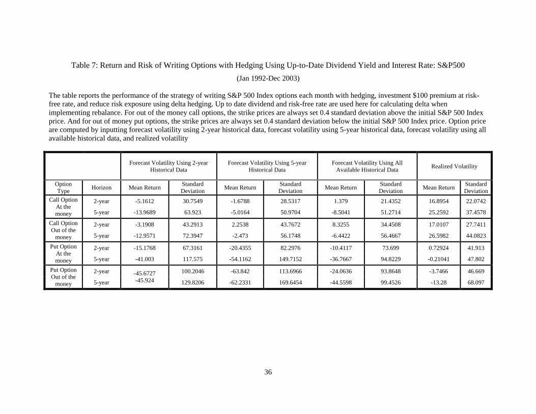
36

Table 7: Return and Risk of Writing Options with Hedging Using Up-to-Date Dividend Yield and Interest Rate: S&P500

(Jan 1992-Dec 2003)

The table reports the performance of the strategy of writing S&P 500 Index options each month with hedging, investment $100 premium at risk-

free rate, and reduce risk exposure using delta hedging. Up to date dividend and risk-free rate are used here for calculating delta when

implementing rebalance. For out of the money call options, the strike prices are always set 0.4 standard deviation above the initial S&P 500 Index

price. And for out of money put options, the strike prices are always set 0.4 standard deviation below the initial S&P 500 Index price. Option price

are computed by inputting forecast volatility using 2-year historical data, forecast volatility using 5-year historical data, forecast volatility using all



Historical Data


Historical Data



Option


Standard


Standard


Standard


Standard

Deviation

Call Option

At the

money

2-year -5.1612 30.7549 -1.6788 28.5317 1.379 21.4352 16.8954 22.0742

5-year -13.9689 63.923 -5.0164 50.9704 -8.5041 51.2714 25.2592 37.4578

Call Option

Out of the

money

2-year -3.1908 43.2913 2.2538 43.7672 8.3255 34.4508 17.0107 27.7411

5-year -12.9571 72.3947 -2.473 56.1748 -6.4422 56.4667 26.5982 44.0823

Put Option

At the

money

2-year -15.1768 67.3161 -20.4355 82.2976 -10.4117 73.699 0.72924 41.913

5-year -41.003 117.575 -54.1162 149.7152 -36.7667 94.8229 -0.21041 47.802

Put Option

Out of the

money

2-year -45.6727

-45.924

100.2046 -63.842 113.6966 -24.0636 93.8648 -3.7466 46.669

5-year 129.8206 -62.2331 169.6454 -44.5598 99.4526 -13.28 68.097

37

Table 8: Effectiveness of Hedging Strategy for S&P 500 Index (Jan 1992-Dec 2003)

The table reports the hedging efficiency in S&P 500 market. In the upper panel, constant dividend and interest rate are used to compute delta in

rebalance, and in the lower panel, up-to-date dividend and interest rate are used. On the left side, the forecast volatility employed is the forecast

volatility with the minimum RSME (forecast volatility using all available historical data for 2-year and 5-year S&P 500 Index options). On the

right side, the realized volatility is applied. Return standard deviations both without and with delta hedging and decrease in standard deviation are

all presented. The decrease in standard deviation is presented as percentile.

Using Forecast Volatility with the Minimum RSME

Using Realized Volatility

Option Type Horizon

Standard Deviation

Without Hedging

Standard Deviation

With Delta Hedging

Decrease in Standard

Deviation (%)

Standard Deviation

Without Hedging

Standard Deviation

With Delta Hedging

Decrease in

Standard

Deviation(%)

Constant

Dividend

and

Interest

Rate

Call Option

At the money

2-year 210.71 21.461 0.8981491

180.0846 14.9933 0.916743

5-year 446.7 16.595 0.9628498

282.8625 17.7577 0.9372214

Call Option

Out of the

money

2-year 261.69 37.909 0.8551378 217.675 16.6057 0.9237133

5-year 519.56 23.344 0.9550697

317.7855 20.0345 0.9369559

Put Option

At the money

2-year 249.02 32.007 0.8714682 200.2548 12.7544 0.936308

5-year 165.33 38.841 0.7650699

190.1894 19.178 0.899164

Put Option

Out of the

money

2-year 334.1 40.39 0.8791081 253.3375 13.732 0.945796

5-year 152.24 54.33 0.6431293

174.5216 25.456 0.854138

Up-to-

Date

Dividend

and

Interest

Rate

Call Option

At the money

2-year 210.71 21.4352 0.8982716 180.0846 22.0742 0.8774232

5-year 446.7 51.2714 0.8852218

282.8625 37.4578 0.8675759

Call Option

Out of the

money

2-year 261.69 34.4508 0.8683526 217.675 27.7411 0.8725573

5-year 519.56 56.4667 0.8913182

317.7855 44.0823 0.8612828

Put Option

At the money

2-year 249.02 73.699 0.7040439 200.2548 41.913 0.7907016

5-year 165.33 94.8229 0.4264628

190.1894 47.802 0.7486611

Put Option

Out of the

money

2-year 334.1 93.8648 0.7190518 253.3375 46.669 0.8157833

5-year 152.24 99.4526 0.346738

174.5216 68.097 0.6098076

38

Table 9: Return and Risk of Writing Options without Hedging: NASDAQ

(Jan 1992-Dec 2003)

The table reports the performance of the strategy of writing NASDAQ Index options each month without hedging and investment $100 premium

at risk-free rate. For out of the money call options, the strike prices are always set 0.4 standard deviation above the initial NASDAQ Index price.

And for out of money put options, the strike prices are always set 0.4 standard deviation below the initial NASDAQ Index price. Option price are



Forecast Volatility Using

2-year Historical Data


5-year Historical Data


All Available Historical Data Realized Volatility



Standard


Standard


Standard

Deviation

Call Option

At the

money

2-year -166.43 244.12 -163.56 260.34 -153.18 227.41 -157.3 195.04

5-year -262.07 479.2 -232.37 423.53 -230.2 391.27 -241.16 388.58

Call Option

Out of the

money

2-year -198.66 308.02 -194.1 330.55 -179.89 284.29 -187.5 236.7

5-year -295.52 543.54 -262.25 481.38 -260.73 442.08 -274.38 441.07

Put Option

At the

money

2-year 44.546 142.14 17.243 204.06 -32.024 317.38 57.919 111.12

5-year 53.173 129.04 14.779 200.88 -4.4791 258.94 68.905 111.76

Put Option

Out of the

money

2-year 34.94 179.25 -6.1066 274.45 -82.742 454.07 54.87 132.03

5-year 62.649 126.53 16.478 216 -10.041 302.77 79.013 113.85

39

Table 10: Return of Risk of Writing Options with Hedging Using Constant Dividend Yield and Interest Rate: NASDAQ

(Jan 1992-Dec 2003)

The table reports the performance of the strategy of writing NASDAQ Index options each month with hedging, investment $100 premium at risk-

free rate, and reduce risk exposure using delta hedging. Constant dividend and risk-free rate are used here for calculating delta when implementing

rebalance. For out of the money call options, the strike prices are always set 0.4 standard deviation above the initial NASDAQ Index price. And

for out of money put options, the strike prices are always set 0.4 standard deviation below the initial NASDAQ Index price. Option price are




Historical Data


Historical Data





Standard


Standard


Standard

Deviation

Call Option

At the

money

2-year 0.65501 34.148 4.2828 40.406 11.422 36.676 0.61368 6.6672

5-year -5.138 35.679 -3.2751 35.529 8.1953 24.609 -4.0346 9.0697

Call Option

Out of the

money

2-year 1.1966 53.982 4.0293 66.155 12.639 58.11 0.57171 10.779

5-year -4.775 49.137 -4.4335 51.068 9.6859 33.439 -4.7506 11.004

Put Option

At the

money

2-year -19.893 67.415 -31.743 89.2 -35.595 84.917 -0.5031 10.349

5-year -46.811 131.46 -48.978 136.26 -50.118 93.772 10.226 18.632

Put Option

Out of the

money

2-year -39.663 100.15 -104.51 140.41 -57.338 120.67 0.12563 12.649

5-year -46.175 151.48 -51.575 151.34 -63.615 115.57 15.42 22.092

40

Table 11: Return and Risk of Writing Options with Hedging Using Up-to-Date Dividend Yield and Interest Rate: NASDAQ

(Jan 1992-Dec 2003)

The table reports the performance of the strategy of writing NASDAQ Index options each month with hedging, investment $100 premium at risk-

free rate, and reduce risk exposure using delta hedging. Up to date dividend and risk-free rate are used here for calculating delta when

implementing rebalance. For out of the money call options, the strike prices are always set 0.4 standard deviation above the initial NASDAQ Index

price. And for out of money put options, the strike prices are always set 0.4 standard deviation below the initial NASDAQ Index price. Option

price are computed by inputting forecast volatility using 2-year historical data, forecast volatility using 5-year historical data, forecast volatility

using all available historical data, and realized volatility


Historical Data


Historical Data



Option


Standard


Standard


Standard


Standard

Deviation

Call

Option

At the

money

2-year 3.85 34.694 6.9547 40.886 13.331 35.018 3.9403 10.756

5-year 8.3001 33.831 7.0938 32.01 21.024 18.162 14.128 29.539

Call

Option

Out of the

money

2-year 4.9718 54.484 7.2748 67.034 15.037 56.866 4.7743 14.767

5-year 10.122 44.66 7.2407 45.761 24.926 24.319 17.092 34.045

Put Option

At the

money

2-year -21.2 71.16 -35.35 95.513 -43.282 99.469 -1.6742 20.667

5-year -60.366 142.95 -71.75 168.07 -85.465 159.41 -8.9997 53.3

Put Option

Out of the

money

2-year -42.109 102.39 -109.79 145.03 -68.975 144.74 -2.1474 25.581

5-year -64.581 160.59 -81.42 188.54 -109.15 199.7 -7.3823 60.017

41

Table 12: Effectiveness of Hedging Strategy for NASDAQ Composite Index (Jan 1992-Dec 2003)

The table reports the hedging efficiency in NASDAQ market. In the upper panel, constant dividend and interest rate are used to compute delta in

rebalance, and in the lower panel, up-to-date dividend and interest rate are used. On the left side, the forecast volatility employed is the forecast

volatility with the minimum RSME (forecast volatility using 2-year historical data for 2-year horizon, and forecast volatility using all available

historical data for 5-year horizon). On the right side, the realized volatility is applied. Return standard deviations both without and with delta

hedging and decrease in standard deviation are all presented. The decrease in standard deviation is presented as percentile.

Using Forecast Volatility with the Minimum RSME

Using Realized Volatility

Option Type Horizon

Standard Deviation

Without Hedging

Standard Deviation

With Delta Hedging

Decrease in

Standard Deviation

Standard Deviation

Without Hedging

Standard Deviation

With Delta Hedging

Decrease in

Standard Deviation

Constant

Dividend

and

Interest

Rate

Call Option

At the money

2-year 244.12 34.148 0.860118

195.04 6.6672 0.9658162

5-year 391.27 24.609 0.9371048

388.58 9.0697 0.9766594

Call Option

Out of the

money

2-year 308.02 53.982 0.8247451

236.7 10.779 0.9544613

5-year 442.08 33.439 0.9243598

441.07 11.004 0.9750516

Put Option

At the money

2-year 142.14 67.415 0.5257141

111.12 10.349 0.9068665

5-year 258.94 93.772 0.6378621

111.76 18.632 0.8332856

Put Option

Out of the

money

2-year 179.25 100.15 0.4412831

132.03 12.649 0.904196

5-year 302.77 115.57 0.6182911

113.85 22.092 0.8059552

Up-to-

Date

Dividend

and

Interest

Rate

Call Option

At the money

2-year 244.12 34.694 0.8578814 195.04 10.756 0.9448523

5-year 391.27 18.162 0.9535819

388.58 29.539 0.9239822

Call Option

Out of the

money

2-year 308.02 54.484 0.8231154

236.7 14.767 0.937613

5-year 442.08 24.319 0.9449896

441.07 34.045 0.9228127

Put Option

At the money

2-year 142.14 71.16 0.4993668

111.12 20.667 0.8140119

5-year 258.94 159.41 0.3843748

111.76 53.3 0.5230852

Put Option

Out of the

money

2-year 179.25 102.39 0.4287866

132.03 25.581 0.8062486

5-year 302.77 199.7 0.3404234

113.85 60.017 0.4728415

42

Table 13: Return & Risk of Writing and Hedging Options with Volatility Markup Using Constant Dividend & Interest Rate: S&P 500

(Jan 1992-Dec 2003)

The table reports the performance of the strategy of writing and delta hedging options each month. Options prices are set by valuing the option

with the appropriate model but with volatility input that is „marked up‟ by 10%, 25%, or 50%. Hedging and hedge rebalance are done with the

unadjusted volatility. Dividend and risk-free rate for calculating delta when implementing rebalance are constant as the initial ones when the

options are write. The table demonstrates the mean return per $100 of option premium, the return standard deviation, the percentage of positions

that lose money.

Option Type Horizon Markup Mean Return Standard

Deviation Loss in %

Option Type Horizon Markup

Mean

Return

Standard

Deviation

Loss

in %

Call Option

At the

money

2-year

1.1 19.2118 20.1178 0.3125

Put Option

At the

money

2-year

1.1 27.731 30.1981 0.3125

1.25 25.7733 18.1325 0.0694

1.25 38.4154 22.7013 0.0764

1.5 34.344 16.3062 0

1.5 50.3821 15.3081 0

5-year

1.1 19.5201 17.7643 0.1597

5-year

1.1 40.146 40.8764 0.1389

1.25 26.0779 16.4359 0.0833

1.25 53.5223 31.3247 0.0833

1.5 34.8888 15.4489 0

1.5 67.6978 22.6267 0

Call Option

Out of the

money

2-year

1.1 30.2462 32.4221 0.2986

Put Option

Out of the

money

2-year

1.1 27.7596 36.743 0.3403

1.25 37.8169 28.4344 0.0625

1.25 41.9651 26.2108 0.0764

1.5 47.0083 24.1352 0

1.5 56.4394 16.5596 0

5-year

1.1 25.7211 23.2321 0.1597

5-year

1.1 45.0436 48.5075 0.1042

1.25 33.1409 21.0836 0.0694

1.25 59.8166 36.4686 0.0833

1.5 42.67 18.9187 0

1.5 74.6229 25.8631 0.0069

43

Table 14:Return & Risk of Writing & Hedging Options with Volatility Markup Using Up-to-Date Dividend & Interest Rate: S&P 500

(Jan 1992-Dec 2003)


with the appropriate model but with a volatility input that is „marked up‟ by 10%, 25%, or 50%. Hedging and hedge rebalance are done with the

unadjusted volatility. Dividend and risk-free rate for calculating delta when implementing rebalance are up to date ones of each month. The table

demonstrates the mean return per $100 of option premium, the return standard deviation, the percentage of positions that lose money.

Option

Type Horizon Markup

Mean

Return

Standard

Deviation Loss in %


Mean

Return

Standard

Deviation

Loss

in %

Call Option

At the

money

2-year

1.1 9.0035 19.9398 0.3056

0.1597

Put Option

At the

money

2-year

1.1 4.6344 62.4999 0.3611

1.25 18.5714 18.2215

1.25 21.236 50.8555 0.2639

1.5 30.9473 16.1198 0.0417

1.5 39.6131 38.8956 0.1458

5-year

1.1 0.6317 44.9227 0.4722

5-year

1.1 -11.6999 89.6787 0.3264

1.25 12.0324 37.6773 0.3819

1.25 14.1791 75.6735 0.2847

1.5 26.7162 29.3858 0.2083

1.5 40.7142 53.4844 0.2083

Call Option

Out of the

money

2-year

1.1 17.9306 31.6377 0.2083

Put Option

Out of the

money

2-year

1.1 -1.7488 75.5385 0.3889

1.25 29.2518 28.2943 0.1458

1.25 20.9624 57.9525 0.2431

1.5 42.8269 24.1613 0.0347

1.5 43.799 41.5135 0.1528

5-year

1.1 4.6231 48.6159 0.4097

5-year

1.1 -13.4135 90.2772 0.3472

1.25 17.8556 40.0306 0.2708

1.25 17.0794 78.1767 0.2917

1.5 34.0472 30.682 0.1528

1.5 46.4561 52.9142 0.2014

44

Table 15:Return & Risk of Writing and Hedging Options with Volatility Markup Using Constant Dividend & Interest Rate: NASDAQ

(Jan 1992-Dec 2003)


with the appropriate model but with a volatility input that is „marked up‟ by 10%, 25%, 50%, 75% or 85%.. Hedging and hedge rebalance are done

with the unadjusted volatility. Dividend and risk-free rate for calculating delta when implementing rebalance are constant as the initial ones when

the options are write. The table demonstrates the mean return per $100 of option premium, the return standard deviation, the percentage of

positions that lose money.

Option

Type Horizon Markup

Mean

Return

Standard

Deviation Loss in %

Option

Type Horizon Markup

Mean

Return

Standard

Deviation

Loss in

%

Call

Option

At the

money

2-year

1.1 -6.1642 32.564 0.44444

Put Option

At the

money

2-year

1.1 -3.0689 56.967 0.375

1.25 -14.931 30.363 0.35417

1.25 15.299 46.006 0.31944

1.5 -26.592 27.145 0.22222

1.5 35.365 34.581 0.26389

1.75 -35.616 24.428 0.048611

1.75 48.27 27.551 0.125

1.85 -38.674 23.462 0

1.85 52.22 25.45 0.041667

5-year

1.1 1.3058 24.252 0.45833

5-year

1.1 -23.75 75.801 0.38194

1.25 -7.8099 23.499 0.34722

1.25 3.8554 58.02 0.35417

1.5 -20.366 21.957 0.26389

1.5 32.53 40.93 0.25

1.75 -30.395 20.336 0.11806

1.75 50.111 31.338 0.16667

1.85 -33.851 19.703 0.041667

1.85 55.351 28.641 0.069444

Call

Option

Out of

the

money

2-year

1.1 -8.0872 49.766 0.44444

Put Option

Out of the

money

2-year

1.1 -12.907 78.199 0.375

1.25 -19.329 44.527 0.35417

1.25 13.692 57.62 0.31944

1.5 -33.237 37.827 0.22222

1.5 39.703 38.845 0.26389

1.75 -43.289 32.821 0.048611

1.75 54.791 28.645 0.125

1.85 -46.57 31.155 0

1.85 59.156 25.797 0.041667

5-year

1.1 1.0874 32.341 0.46528

5-year

1.1 -29.74 90.143 0.36806

1.25 -9.8568 30.581 0.40972

1.25 3.8711 66.243 0.29861

1.5 -24.241 27.675 0.14583

1.5 36.644 44.596 0.27778

1.75 -35.239 25.028 0.055556

1.75 55.585 33.095 0.069444

1.85 -38.939 24.06 0.020833

1.85 61.052 29.957 0.027778

45

Table 16:Return &Risk of Writing &Hedging Options with Volatility Markup using Up-to-Date Dividend and Interest rate: NASDAQ

(Jan 1992-Dec 2003)


with the appropriate model but with a volatility input that is „marked up‟ by 10%, 25%, 50%, 75% or 85%. Hedging and hedge rebalance are done

with the unadjusted volatility. Dividend and risk-free rate for calculating delta when implementing rebalance are up to date ones of each month.

The table demonstrates the mean return per $100 of option premium, the return standard deviation, the percentage of positions that lose money.

Option

Type Horizon Markup

Mean

Return

Standard

Deviation Loss in %


Mean

Return

Standard

Deviation

Loss in

%

Call

Option

At the

money

2-year

1.1 -3.1607 33.046 0.47917

Put Option

At the

money

2-year

1.1 -4.293 60.489 0.80556

1.25 -12.173 30.768 0.34722

1.25 14.175 49.252 0.53472

1.5 -24.16 27.456 0.24306

1.5 34.363 37.486 0.25

1.75 -33.436 24.675 0.11111

1.75 47.353 30.215 0.083333

1.85 -36.579 23.689 0.013889

1.85 51.33 28.039 0.013889

5-year

1.1 13.089 16.973 0.47222

5-year

1.1 -53.203 130.98 0.72917

1.25 2.7038 15.846 0.36806

1.25 -19.649 102.76 0.48611

1.5 -11.415 14.771 0.26389

1.5 14.932 75.374 0.25

1.75 -22.558 14.068 0.15278

1.75 35.979 59.687 0.125

1.85 -26.373 13.829 0.076389

1.85 42.227 55.192 0.069444

Call

Option

Out of

the

money

2-year

1.1 -4.6346 50.208 0.47222

Put Option

Out of the

money

2-year

1.1 -15.052 80.337 0.43056

1.25 -16.262 44.9 0.38194

1.25 11.867 59.623 0.38194

1.5 -30.637 38.123 0.25

1.5 38.216 40.68 0.31944

1.75 -41.022 33.066 0.069444

1.75 53.512 30.363 0.29861

1.85 -44.411 31.385 0.020833

1.85 57.94 27.48 0.28472

5-year

1.1 14.839 22.981 0.49306

5-year

1.1 -66.367 158.16 0.44444

1.25 2.1595 21.58 0.45139

1.25 -24.214 119.08 0.36806

1.5 -14.263 19.941 0.18056

1.5 16.543 83.419 0.3125

1.75 -26.653 18.663 0.048611

1.75 39.914 64.138 0.29861

1.85 -30.791 18.21 0.034722

1.85 46.631 58.781 0.25

46

Bibliography

Black, F., & Sholes, M. (1973). The pricing of options and corporate liabilities. Journal of

Political Economy 4 , 637-659.

Figlewski, S. (1998). Derivative Risk, old and new. Brookings-Wharton Papers on Financial

Serviceb1 , 159-217.

Figlewski, S., & Green, T. C. (1999). Market Risk and Model Risk for a Financial Institution

Writing Options. Journal of Finance Vol 54 Issue 4 , 1465-1499.

Jorion, P. (2007). Value at Risk:The New Benchmark for Managing Financial Risk. New York:

McGraw-Hill.

L.McDonald, R. (2006). Derivatives Market. New York: Pearson Education,Inc.

Merton, R. C. (1973). Theory of Rational Option Pricing. Bell Journal of Economics and

Managment Science 4 , 141-183.

model risk and market risk in derivative trading

Documents