Modeling of Crowd Behavior

The Creation of a Program to Predict the Movements of

Individuals within a Crowd

A Major Qualifying Project Report to be submitted to the faculty of

Worcester Polytechnic Institute in partial fulfillment of the requirements for the

Degree of

Bachelor of Science

Submitted by:

Brendon Dubois

Brendon Willey

Submitted to:

Project Advisor:

Prof. Grétar Tryggvason

April 24, 2008

ii

Abstract

Traditionally thought to be erratic and unpredictable, the prediction of crowd movements has

been difficult and inaccurate. Following the original works of Dirk Helbing, this project has

created a system with which crowd behaviors and movements can be mapped and predicted.

By adding obstacles to his model, we have simulated a more real world environment. With

the aid of this system, it may be possible to find ways to decrease the life-threatening dangers

that naturally arise within the existence of crowds.

iii

Acknowledgments

For their help and guidance throughout the project, this team would like to thank the

following:

Professor Jim Doyle

Adriana Hera

Professor Grétar Tryggvason

iv

Table of Contents

Abstract ........................................................................................................................................... ii

Acknowledgments.......................................................................................................................... iii

Table of Contents ........................................................................................................................... iv

Table of Figures .............................................................................................................................. v

1 Introduction ............................................................................................................................. 1

2 Background ............................................................................................................................. 3

2.1 Defining Panic ............................................................................................................ 3

2.2 Why Stress Effects Crowds ........................................................................................ 5

2.3 History of Crowd Modeling ....................................................................................... 5

2.3.1 Particle Models ................................................................................................... 6

2.3.2 Continuum Models.............................................................................................. 7

3 Methodology ......................................................................................................................... 11

3.1 Helbing, Farkas, and Vicsek Model ......................................................................... 11

3.2 Incorporating Obstacles in Helbing, Farkas, and Vicsek‟s Model ........................... 15

3.3 Evaluating Parameter Changes................................................................................. 19

4 Results and Analysis ............................................................................................................. 24

4.1 Validating Case ........................................................................................................ 24

4.2 Addition of Obstacles ............................................................................................... 27

4.2.1 Test One- Empty Room .................................................................................... 28

4.2.2 Test Two - Randomly Placed Obstacles ........................................................... 31

4.2.3 Test Three- Line of Objects in center of the room............................................ 35

5 Recommendations and Conclusions ..................................................................................... 39

5.1 The Decision Rule .................................................................................................... 39

5.2 Future Tests .............................................................................................................. 41

6 Works Cited .......................................................................................................................... 44

7 Appendix A- The Code ......................................................................................................... 45

v

Table of Figures

Figure 1 -Variations in parameter Bi ...................................................................................... 13

Figure 2 - Gradient grid .......................................................................................................... 17

Figure 3 - Contour plot of the distance function for three obstacles ...................................... 18

Figure 4 - 3-D representation of the room .............................................................................. 19

Figure 5 - Various magnitudes of repulsion forces ................................................................. 20

Figure 6 - Repulsion force equal to 2000N ............................................................................. 21

Figure 7 - Repulsion force equal to 9000N ............................................................................. 22

Figure 8 - Crowd movement over 9 seconds .......................................................................... 26

Figure 9 - Crowd movement under simulated panic ............................................................... 27

Figure 10 – Number of People That Have Exited Versus Time with no obstacles, 2 m/s

desired velocity ....................................................................................................................... 29

Figure 11 - Effects of changes in desired velocity .................................................................. 29

Figure 12 – Number of People That Have Exited Versus Time with no obstacles, 5 m/s

desired velocity ....................................................................................................................... 30

Figure 13 - Distance Function Contour Plot with 4 Obstacles ............................................... 32

Figure 14 – Number of People That Have Exited Versus Time with Four Obstacles, 5 m/s

Desired Velocity ..................................................................................................................... 33

Figure 15 - Distance function contour plot with 3 objects ...................................................... 35

Figure 16 - Distance function contour plot with 1 object ....................................................... 37

1

1 Introduction

People, by nature, are a social being, enjoying the interactions of others. But a

number of things can drastically change an enjoyable experience to one that kills thousands

of people each year. One of the most life-threatening of mass human interactions is a crowd

stampede. Traditionally believed to be unpredictable, a stampede can often increase the

problems that caused the original life threatening situation. The idea that crowds are

irrational, and thereby unpredictable, comes from early sociological writings by aristocrats

during the French Revolution of the 1790‟s (3)

. However, the present sociological perception

of crowds is that they are rational, as long as they are calm. Once a traumatic or life-

threatening event occurs, all sense of rationality seems to be lost.

So what happens to the minds of individuals during a chaotic experience? In a calm

situation, people seem to be rational with an ability to think. An increase of people in a

crowd is not synonymous with a loss of rational thought. A simple look at a New York City

street during rush hour is an example of a massive amount of people that seem to flow

smoothly. So why is it that during an event people seem to lose the ability to think? It could

be a question of physiology. However it could be possible to predict the motions of this

seemingly erratic a crowd.

It seems that many characteristics of escape panics parallel the characteristics of

particle interactions. Particles bouncing off each other, for example, are similar to people

pushing and fighting to escape. Our project uses this idea to mimic the motions of the

individuals in the crowd as self-serving particles. We have designed a program that simulates

2

people moving within a closed area. After introducing initial conditions the people are able to

move around the enclosed are freely. All the people have the task of moving across the area

toward the “door” in an attempt to escape. By adding obstacles for the people to avoid, the

hope is that we can find ways to increase the flow through the “door” and minimize the

bottleneck effect.

3

2 Background

The background section of this report is dedicated to introducing the reader to the basic

ideas that surround this project. This section will discuss historical interpretation of the

movements of crowds. This section will discuss what other researchers have done in order to

predict crowd movements and will look at the current benefits that exist by making such

predictions.

One way in which to analyze the movements of crowds is to realize that the

movements of individuals within the crowd share some of the same characteristics as the

movements of particles. When properly constructed, creating a program that can simulate the

seemingly random movements of particles will give insight to the movements of people in a

crowd.

2.1 Defining Panic

Before we can begin to study the behaviors of crowds in panic, it is first important to

fully define what panic is. Many articles define “panic” differently. This fact makes it

difficult to clearly identify the issue of panic simply due to the seemingly wide variety of

definitions. Quarantelli (7)

writes that to characterize panic, as is frequently done, as

irrational, antisocial, impulsive, non-functional, maladaptive, and inappropriate is of little

assistance in classifying a particular individual or mass act. These terms do not seem to

isolate a single behavioral entity. Also, Quarantelli asks what induces panic.

4

In order to further understand what goes on in the mind of those in a crisis situation,

many people have been interviewed on their thoughts and feelings during what they

described to be a life threatening situation. It is clear that the most obvious observation of a

panic situation is people running or trying to get away as fast as possible. Simply put, people

do their best to make their way as far from a life-threatening situation as possible in the

direction of the nearest exit.

People find their way to the nearest exit in two ways, according to Quarantelli. The

first is a habitual pattern; this exit is one that the individual knows well and uses frequently.

However, this may not be the nearest or even safest exit. The second way an individual finds

an exit is by following others who are already in flight. People have a natural tendency to

follow others.

In his findings Quarantelli states that panic flight represents individualistic behavior.

He cites that there is no unity of action, no co-operation with others, and no joint activity by

the members of the mass. It seems that there is a complete breakdown of cooperative

behavior amongst individuals within a crowd.

It also seems that people in a life-threatening situation do not seem to take into

consideration what is currently happening, but what may happen in the immediate future. In

an interview with Quarantelli, a gentleman says “This thing seemed to me as if it was coming

right at me. I ran like a scared rabbit across the street. All I was thinking was that this big ball

of gasoline was coming down on top of me and I was making a run in order to get away from

it. I was thinking to myself, I wonder if any part of this is going to hit me.”

5

It seems that many things affect the mindset of individuals in a life-threatening

situation. The following section will discuss how stress affects a crowd as a whole.

2.2 Why Stress Effects Crowds

A study at the University of Delaware sites that many of the irrational tendencies of a

crowd stem from the environments and experiences of people within the crowd.(6)

It is noted

that literary articles that describe people in disastrous situations may have a negative impact

on the decision making abilities of individuals when they themselves experience a similar

disaster. It has been observed that many people believe one of two things in a disastrous

situation: Either they are in the worst possible situation and are going to die or they expect

there to be a “hero”, as in a book or a movie.

Similarly, newspaper articles seem to, more often than not, stress the dangers of a

situation rather than the more positive aspects, such as a “hero” or the many lives that were

spared. These prior experiences, combined with the stress of the situation itself, seem to be

the source of the irrational thought that can arise from a life-threatening situation.

2.3 History of Crowd Modeling

It seems to be a generally accepted misconception that a crowd, as one unit, is not a

rational thinking body; that it is irrational and erratic and therefore making its actions and

movements unpredictable and non-calculable. As stated previously, the idea of irrationality

comes from the early sociological writings by aristocrats during the French Revolution of the

6

1790s (3)

. However, recent studies have shown that a crowd, as one unit, does in fact act

rationally.

By studying the movements of a crowd through simple observation, it is easy to

observe a self-organized, bidirectional, flow (8)

. Without any instruction, individuals within

the crowd seem to organize and move with limited or no friction between other individuals.

At a bottleneck, it has been observed that individuals traveling in opposite directions will

move aside to allow other people to pass, thereby allowing flow in both directions. So, why,

when a stress is introduced to a crowd, do these crowd behaviors change to behaviors that

seem disorganized and illogical?

2.3.1 Particle Models

In September of 2000, Professor Dirk Helbing published in the Journal “Nature” his

works in the area of simulating the dynamical features of escape panic. With one of the

largest archives of catastrophe videos in Europe, Helbing seems to be the most versed in the

modeling and simulation of crowds and their behavior. His work has inspired many other

articles to be written and much more research to be done.

Helbing writes that streams of pedestrians follow physical laws very similar to the flow

characteristics of liquids and gasses (9)

. He writes that the characteristic features of escape

panics can be summarized as follows: (1) People move or try to move considerably faster

than normal. (2) Individuals start pushing, and interactions among people become physical in

nature. (3) Moving and, in particular, passing of a bottleneck becomes uncoordinated. (4) At

exits, arching and clogging are observed. (5) Jams build up. (6) The physical interactions in

7

the jammed crowd add up and cause dangerous pressures of up to 4,450 N m-1

which can

bend steel barriers or push down brick walls. (7) Escape is further slowed by fallen or injured

people acting as „obstacles‟. (8) People show a tendency towards mass behavior, that is, to do

what other people do. (9) Alternative exits are often overlooked or not efficiently used in

escape situations (2)

. These observations are essential to his work because they allow him to

characterize individuals as particles and, in turn, allow him to write computer based models

that can simulate the behavior of people as particles.

Although he cannot simulate an actual event in his computer based model, due to the

fact that the events he would be mimicking are unexpected and unpredictable, he can assign a

series of parameters to his program. These limiting parameters include, but are not limited to,

actual versus desired velocity and reasonable accelerations. Helbing includes both the force

interactions from particle to particle as well as from particle to walls.

By writing computer programs in this fashion, Helbing has been able to simulate and

reproduce many observed past phenomenal crowd behaviors (2)

. His work has been used to

test the efficiency at which people can escape buildings, arenas, and other areas where

humans congregate.

2.3.2 Continuum Models

It has long been the belief that a crowd is an irrational and seemingly randomly moving

body, but what if a crowd, as one unit, has the ability to think? In a writing published in the

Annual Reviews of Fluid Mechanics titled “The Flow of Human Crowds”, Roger L. Hughes

writes that many sociological issues arise in studying the behavior of crowds, but the present

8

study is concerned only with the factors affecting their motion. (3)

Hughes credits Helbing

with his extraordinary work on modeling crowd motion as individuals within a larger body

with the scope of practical applications, but he feels that as a research tool, it is missing the

ability to tract numerical data and therefore not useful in getting results. He also feels that

Helbing‟s approach does not satisfy the representation of a crowd as a whole, but rather the

individuals within the crowd.

Hughes believes that a crowd of individuals can be represented as a “continuum”. He

says, however, that in order to model a crowd of individuals in this way the distance from

pedestrian to pedestrian must be significantly smaller that the distance from the pedestrians

to the area in which they move.

The next issue that must be addressed is the individual characteristics from pedestrian to

pedestrian; that is to say, all the pedestrians are different in some way and therefore cannot

be models as equal. In order to address the issue, Hughes has made three hypothesis:

Hypothesis 1. The speed at which pedestrians walk is determined solely by the

density of surrounding pedestrians, the behavioral characteristics of the

pedestrians, and the ground on which they walk.

Hypothesis 2. Pedestrians have a common sense of the task (called potential)

that they face to reach their common destination, such that any two

individuals at different locations having the same potential would see no

advantage to exchange places.

9

Hypothesis 3. Pedestrians seek to minimize their (accurately) estimated travel

time but temper this behavior to avoid extreme densities. This tempering is

assumed to be separable, such that pedestrians minimize the product of their

travel time as a function of density.

Hypothesis 1 does a good job of explaining how two pedestrians walking in the same

direction toward the same location may experience different travel time due to the terrain.

For example, a person walking up a slope would move slower lineally than a person walking

on a horizontal surface. By assuming hypothesis 2 to be accurate, you assume that people are

satisfied with their location within the crowd. If, for example, you have a series of tall people

surrounding a smaller person, the small person can gauge his direction based on the taller

people, thereby eliminating the need for the smaller person to visualize an exit. Hypothesis 3

states that a person will take the most direct route to a desired location without sacrificing

their reaching the location by walking through a thick crowd. Hughes realizes there is no

evidence that suggests that people minimize their travel time as a function of density. He

simply assumes this for simplicity.

These hypotheses allowed Hughes to derive the following equations:

0)()()()( 22

yfg

yxfg

xt

22

1)()(

yx

fg

10

Where φ is the remaining travel time, which is a measure of the remaining task, ρ is the

density of the crowd, ƒ(ρ) is the speed of pedestrians as a function of density, g(ρ) is a factor

related to the discomfort of the crowd at a given density, and (x, y, t) denotes the horizontal

space and time coordinates.(3)

Hughes has used his works to make suggestions to situations that have seen mass

crowd disasters in the past. In 1990, during the annual Muslim Hajj, 1426 pilgrims lost their

lives on the Jamarat Bridge. Hughes used his hypothesis and set of equations to make

recommendations regarding an improvement for the crowd flow of individuals during this

religious time.

11

3 Methodology

This project‟s objective was to write a program that could predict the movements of

individuals within a crowd by modeling them as particles. We wrote a program in Matlab

that can be used to simulate the forces on the “particles” as they interact with each other and

the environment. The team has created a series of objectives that were followed to ensure that

it was successful in meeting its target objective. The goals for this project were to:

Create a program that can simulate particle movement and interactions

Run the program to search for movement patterns that can be used in

predictions

Predict the movement of particles, paralleling people

Make recommendations that can improve the crowd flow of

individuals when exiting a room.

Once we had created the program, we needed to test our model to ensure that it produced the

same results as the previous works of Helbing.

3.1 Helbing, Farkas, and Vicsek Model

Our computer model simulates crowd dynamics of pedestrians based on a generalized

force model (1)

. The model allows us to observe the forces pedestrians exert on each other

and the corresponding build up of pressure at an exit during a panic situation. Our model is

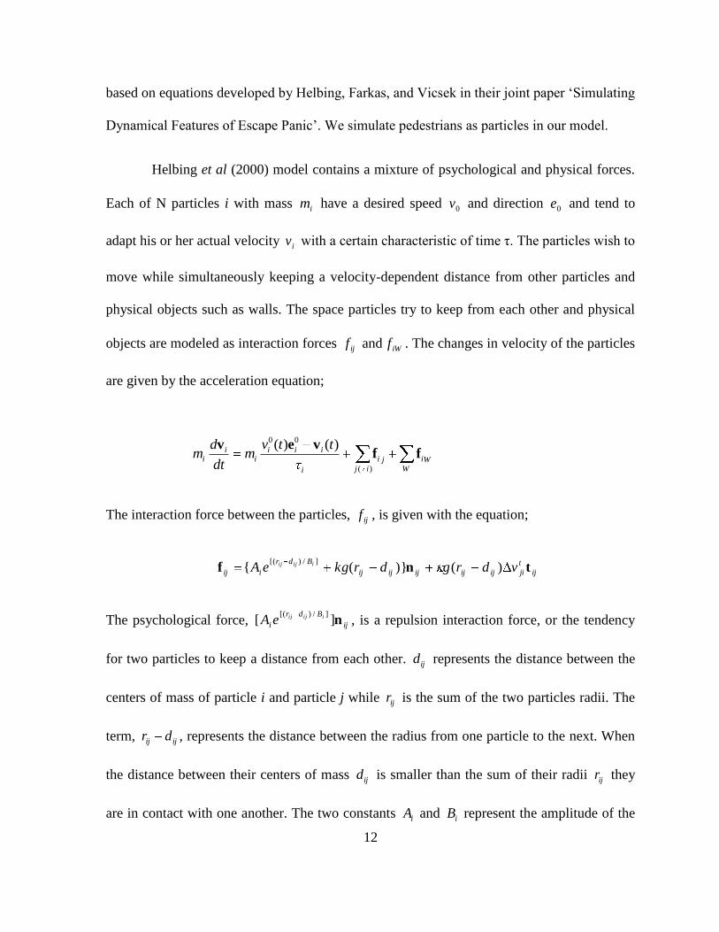
12

based on equations developed by Helbing, Farkas, and Vicsek in their joint paper „Simulating

Dynamical Features of Escape Panic‟. We simulate pedestrians as particles in our model.

Helbing et al (2000) model contains a mixture of psychological and physical forces.

Each of N particles i with mass im have a desired speed 0v and direction 0e and tend to

adapt his or her actual velocity iv with a certain characteristic of time τ. The particles wish to

move while simultaneously keeping a velocity-dependent distance from other particles and

physical objects such as walls. The space particles try to keep from each other and physical

objects are modeled as interaction forces ijf and iWf . The changes in velocity of the particles

are given by the acceleration equation;

The interaction force between the particles, ijf , is given with the equation;

ij

t

jiijijijijij

Bdr

iij vdrgdrkgeA iijij tnf )()}({]/)[(

The psychological force, ij

Bdr

iiijijeA n][]/)[(

, is a repulsion interaction force, or the tendency

for two particles to keep a distance from each other. ijd represents the distance between the

centers of mass of particle i and particle j while ijr is the sum of the two particles radii. The

term, ijij dr , represents the distance between the radius from one particle to the next. When

the distance between their centers of mass ijd is smaller than the sum of their radii ijr they

are in contact with one another. The two constants iA and iB represent the amplitude of the

WWi

ijji

i

iiii

ii

ttvm

dt

dm ff

vev

)(

00 )()(

13

repulsion force and how quickly the force decays respectively. iB determines how concerned

the particles are with one another based on their distance apart. Taking the value for iB that

Helbing et al uses in his simulation, 0.08m, we can see the effect it has in the interaction.

Figure 1 -Variations in parameter Bi

Taking x to represent the distance between the two particles and f to be the resulting

force, the graph in Figure 1 shows the effect that changing the value of iB can have. The

distance, x, is plotted along the x-axis and the force, f, is plotted along the y-axis. The red

line represents a small iB value and the green line a much higher value. You can see from

the graph that a larger iB will allow the forces to get much closer to one another before they

feel any concern towards another particle.

At distances greater than roughly 0.5 meters the force has negligible effect on the

motion of the particles. Two people do not seem to have a tendency to increase their distance

from one another if a sufficient distance, greater than one meter, already separates them.

14

Increasing the value of this constant will essentially increase the particles awareness of one

another. The constant iA can be chosen as to represent a reasonable force value pertaining

when two particles are in direct contact with one another or when 0ijij dr . The value we

will use for our experiments will be NAi

3102 as taken from Helbing et al.

The next two terms in the equation, )( ijij drkg and ij

t

jiijij vdrg t)( physical

forces. They represent the force that counteracts body compression when they come in

contact, and the sliding friction force that impedes relative tangential motion respectively.

These two terms only effect the motion of the particles when they come into contact with one

another and are controlled by the function )(xg . When ijij dr , the particles are not in

contact with one another, 0)(xg and the two terms above have no effect on the motion of

the particles. When the opposite is true, ijij dr , 1)(xg and the two terms effect the

motion. The parameters k and determine the obstruction effects in the physical

interactions and have units of 2kgs and 11skgm respectively. The parameter k will

determine the magnitude of the compression force in the direction pointing directly from

particle i to particle j. The parameter determines the magnitude of the friction impeding

tangential motion between the two particles. The values we will use for these parameters are

2kgsk and 11skgm . These values are taken directly from the Helbing, et al model.

The interaction the particles have with the wall is equivalent the interactions with one

another. The resulting equation is

iWiWiiWiiWiWi

Bdr

iiW drgdrkgeA iiWi ttvnf ))(()}({]/)[(

15

iWd being the distance from the particle to the wall, iWn the direction perpendicular to the

wall, and iWt the direction tangential to it. The three terms in this equation are analogous to

the three terms in the particle interaction equation. iW

Bdr

iiiWieA n)(

/)( represents the

psychological tendency for particles to avoid the wall, )( iWi drkg counteracts body

compression in the direction normal to the wall, and iWiiWi drg tv)(( ) represents the

sliding friction force the particle will experience if the particle hits the wall from any

direction except directly normal to it. The constant values used for the wall interactions will

be the same as those used in the particle interaction equation and are all taken directly from

Helbing et al.

3.2 Incorporating Obstacles in Helbing, Farkas, and Vicsek’s Model

The influence of walls and obstacles on the motion of people is, of course, one of the

aspects that the model of Helbing et al is particularly well suited for. Incorporating a complex

geometry in the original model is, however, fairly complex and computationally intensive.

Since the geometry does not usually change, there are considerable opportunities to make the

computations more efficient. Here we develop a methodology where the distance from the

walls is computed once and for all for every point in the computational domain. The wall

force on each particle is then found at each time step by interpolating the distance, as well as

the direction to the wall. This greatly simplifies the computation of the wall force and allows

the incorporation of arbitrarily complex domains.

16

Particle interactions with the wall and other particles will be governed by the Helbing

et al equations. Particles, of universal mass and radii, will be placed in a rectangular room

containing various obstructive objects. The particles will all try to leave the room through

various exits and interact with the wall, the obstacles, and each other on the way out. In this

way we will be able to examine how the configuration of various obstacles will affect the

flow of particles through the exit.

In order for the particles to interact with the walls and the obstacles in the room they

must be aware of their distance from each of them. To do so we calculate distance functions

for each particle from the walls and obstacles. The specifics of the particles interactions with

the wall are explained in section 4.1, Evaluating Parameter Changes.

The room is divided up into xm by ym segments with the overall length and width of

the room being xL and yL respectively. Objects will be placed within this grid and the

distance ),( jid from the objects can be calculated at every grid point. Given the distance

function we can calculate the gradient ),( dydx at each grid point by

xhjidjidjidx 2/)],1(),1([),(

yhjidjidjidy 2/)]1,()1,([),(

where xh and yh represent the dimensions of grid segment in the x and y directions

respectively.

17

Once the gradient at each grid point is known the particles can be placed within the

grid. The gradient of each particle will then be calculated using an area weighting operation

within each grid block

Figure 2 - Gradient grid

where each grid block is divided into four areas each with their common corner at the

particle. Once these areas are calculated the gradient at the particle ),( pp dydx can be

calculated by;

),1(*4),(*3)1,(*2)1,1(*1 jidxAjidxAjidxAjidxAdx p

),1(*4),(*3)1,(*2)1,1(*1 jidyAjidyAjidyAjidyAdy p

18

The gradient of the particle ),( pp dydx calculated in this way is equivalent to iWn in the

Helbing et al equations. Similarly the distance from the particle to the wall iWd can be

calculated with

),1(*4),(*3)1,(*2)1,1(*1 jidAjidAjidAjidAdiW

0 2 4 6 8 100

1

2

3

4

5

6

7

8

9

10

Figure 3 - Contour plot of the distance function for three obstacles

Figure 3 shows the contours of the distance function for a ten by ten meter room with

a wall with an opening and three obstacles placed at random locations. The dark blue circles

represent the exact size and placement of the three obstacles while the straight line represents

the wall with the break being the doorway.

19

The particles were tested with various sized rooms and obstacle locations. The

particles were placed in random locations within a given room and will try to exit through the

door on the right side.

0

2

4

6

8

10

0

2

4

6

8

10

0

1

2

3

Figure 4 - 3-D representation of the room

Figure 4 above shows a three dimensional representation of a ten by ten meter room

containing forty particles. The blue line represents a wall with the break in the line being the

doorway through which the particles will pass.

3.3 Evaluating Parameter Changes

Before we began our main tests we analyzed how the motion of the particles is

affected if the parameters are altered. We began by looking at the parameters that effect the

20

particle‟s interactions with one another. The equation that governs the particles

psychological tendency to avoid one another, ij

Bdr

iiijijeA n][

/)(, depends mainly on the

distance between the two particles centers of mass, ijij dr . The parameters iA and iB can

be changed in order to manipulate the specifics of this interaction.

The first parameter, iA , determines the magnitude of the repulsion force and has units

of Newton‟s, N. Increasing the value of this parameter will increase the force that the

particles exert on one another once they get sufficiently close to each other. Since this force

is purely psychological and not physical in nature, this parameter simulates how greatly the

particles want to stay away from one another once their separation has decreased to a certain

value. The following figure represents three different iA values:

Figure 5 - Various magnitudes of repulsion forces

21

The x-value is the distance between two particles. When x=0 the particles are touching. The

y-intercept represents the magnitude of force the two particles would exert on each other. In

this case, iA is 1000N, 2000N, and 500N. This graph demonstrates that by increasing the

iA value, the magnitude of the force between the two particles is increased and therefore will

have a stronger desire to avoid each other.

Another way we were able to visualize how the iA value affects our particles was to

change the iA value within our program. The following two figures were derived using the

exact same parameters, save the iA values. Figure 6 has an iA value of 2000N and Figure 7

has an iA value of 9000N.

Figure 6 - Repulsion force equal to 2000N

22

Figure 7 - Repulsion force equal to 9000N

The blue line represents the wall. The left side of the blue line is inside of the room and the

right side is the outside. 2000N was chosen to represent the iA value because it is the value

we used in our tests. We chose 9000N for the second iA value because it could be compared

well to the 2000N. It is clear to see that with an increase of iA parameter the particles have

greater tendencies to stay as far away from each other as possible.

The parameter, iB determines the rate at which the function of the repulsion force will

decay. Changing the value of this parameter will determine how close the particles can come

to one another without feeling the repulsion force. Decreasing the value of iB , or increasing

the value of the exponent will allow the particles to get closer to one another before feeling

any repulsion. This parameter essentially sets a value for how close the particles are willing

to get to one another before they feel the need to back away.

23

The psychological tendency for the particles to stay away from the wall and the

obstacles, iW

Bdr

iiiWieA n][]/)[(

, is essentially the same as the equation for them to stay away

from one another except that it depends on each individual particles distance from the walls

and the obstacles. The parameters governing the particle interactions with one another are the

same as used for the wall and obstacle interactions.

These parameters can all be manipulated as shown in order to more realistically

reproduce actual human interactions. These values could be changed depending on the

desired velocities. During a panic situation with s

mvi 50 the particles may get closer to one

another before the desire to separate occurs. For normal desired velocities, s

mvi 10 ,

Helbing et al suggest setting iA =2000N, and iB =0.08m in order to reproduce distance that

individuals keep from one another.(5)

For this project we will use the parameters given in

Helbing et al model, and shown above, for all tests regardless of the desired velocities for

simplicity. Reasonable variations in the parameters do not seem to effect the particles

interactions too greatly so they will be kept constant too avoid over-complicating the

problem. Parameter changes may want to be considered for future projects.

24

4 Results and Analysis

In order to successfully write a program that could predict the movements of

individuals within a crowd by modeling them after particles, we had to develop objectives

that clearly defined our goals. The following four objectives are what we used as a road map

to guide us throughout the project. Our goals were to create a program that could simulate the

movements of crowds, run the program to search for movement patterns, predict the

movements of particles, and make recommendations on how to improve our model and

possibly the way crowds move. The following sections clearly describe the results of the

steps descried in the Methodology that we took to meet these objectives.

4.1 Validating Case

In order to test if our program was created properly it was essential for us to first

reproduce Helbing et al findings, specifically the arch-shaped clogging at the doorway using

their exact parameters. We thus selected the mass of the particles, m= 80kg, and the

constants iA =2 X 103N and iB =0.08m. The parameters

ms

kg5104.2 and 2

5102.1s

kgk

set the obstruction effects when the particles come into contact with the walls, obstacles, or

one another. Helbing et al used particles with various diameters, [0.5m 0.7m], in order to

simulate varying shoulder width in a crowd and add an amount of irregularity to the model.

This would add irregularity to the model in order to avoid possible symmetrical interactions

between the crowd on the left and right side of the doorway. (5)

Our model will use a

constant value of 0.5 meters for the shoulder width of all the individuals. We will eliminate

possibilities for this symmetry by giving the people random starting positions and in later

25

tests with the incorporation of obstacles. For this simulation there were no objects in the

confined space and the particles were able to move freely with other particles and the walls

being their only obstacles.

The first of Helbing et al tests were to simulate the flow of individuals under normal

conditions, s

mvi 8.00 . They found that 0.73 persons per second exited through the doorway.

Our simulation was run for thirty seconds and twenty four people escaped giving a rate of 0.8

people per second. This value is relatively close to the results of Helbing et al result and the

difference may be accounted for in the differences in shoulder width between our simulations

and theirs.

26

Figure 8 - Crowd movement over 9 seconds

Figure 8 shows top-view snapshots of this simulation at intervals of one second. The

blue line represents a wall with the small break in it being the doorway. The people move

toward the door and seem to wait their turn to exit the door. The particles are not coming into

contact with one another since this low desired velocity does not represent a panic situation

but a normal one. The flow of people through the door remains steady throughout the

simulation. This test would most accurately depict people leaving a large stadium after a

concert or sporting event.

The second of the tests simulates the particles motion in a panic situation with desired

velocity, s

mvi 0.50 . According to Helbing et al the interactions amongst the people should

become more physical, producing clogging at the exit and creating non-steady flow of people

through the doorway. The clogging is due to the people rubbing against one another as they

fight to get through the door.

27

0 1 2 3 4 5 6 7 8 9 100

1

2

3

4

5

6

7

8

9

10

Figure 9 - Crowd movement under simulated panic

Figure 9 shows the clogging effect in a panic simulation. In contrast to the

interactions in figure 8, the people here are bunched more closely together as their desire to

escape has overcome their psychological tendency to keep a certain distance between one

another. The clogging causes the arch-like blockage at the doorway. Once the blockage takes

place flow through the doorway stops until the arch breaks and people can escape again. This

results in short bursts of people flowing through the door separated by intervals in which

flow stops completely.

4.2 Addition of Obstacles

To extend the model of Helbing‟s et al, we added various obstacles into the room and

examine the crowds movements around them. The addition of obstacles will simulate a more

realistic room configuration, as few rooms where a crowd would gather are completely

28

empty, and give insight into how various configurations of obstacles could help to decrease

the clogging factor.

These tests will examine crowd movements in three different room configurations.

The first test will be run in an empty room and used later to be compared with rooms

containing obstacles. The next two tests will examine various configurations of obstacles.

Parameter values as discussed in the methodology will remain constant through each test to

reduce the complexity of the problem. Each test will examine crowds of 40 people and each

will be run for 15 seconds.

Each room configuration will be tested multiple times with different desired

velocities for the people. The magnitude of velocities to be used for each room configuration,

1 m/s, 2 m/s, and 5 m/s, will represent normal non-panic conditions, nervous conditions and

extreme panic conditions, respectively.

4.2.1 Test One- Empty Room

The Helbing et al experiment found that once the desired velocities, 0

iv reached 1.5 m/s

the rate at which people exited the room decreased. However, our findings did not show the

exact same phenomenon. In fact, we found that with an increase of desired velocity, up to

approximately 4 m/s, the rate at which people could exit increased and the outflow remained

steady.

29

0 500 1000 1500 2000 2500 3000 35000

5

10

15

20

25

Time

People

Escaped

Figure 10 – Number of People That Have Exited Versus Time with no obstacles, 2 m/s desired velocity

This figure represents the number of particles that have exited the room per second. The

desired velocity is set to 2 m/s for each particle, just above the Helbing et al limit of 1.5 m/s.

The flow of individuals through the door is appears to be relatively steady contrary to the

Helbing at al simulation. This was observed for desired velocities up to approximately 4 m/s

at which point outflow became non-steady and the rate at which persons escaped per second

began to decrease with increasing desired velocity.

0

0.2

0.4

0.6

0.8

1

1.2

1.4

1.6

1.8

2

1 2 3 4 5 6 7 8 9 10

Desired Velocity (m/s)

Ou

tflo

w (

pers

on

s/s

)

Series1

Figure 11 - Effects of changes in desired velocity

30

Figure 11 illustrates this phenomenon. Increasing the desired velocity results in the people

exerting greater physical forces on each other around the exit. The arch-like blockages

around doorway take longer to break resulting in greater amounts of time between bursts of

people through the door.

Figure 12 – Number of People That Have Exited Versus Time with no obstacles, 5 m/s desired velocity

The intervals in time in which the arch-like blockage forms at the doorway can be seen in

figure 12. The plateaus seen on the graph after the fourth, tenth, and fifteenth particles pass

through the door represent the times that the arch-like blockage occurs.

This model clearly shows the clogging at the doorways that the particles experience,

just as Helbing et al described. Their model produced clogging and irregular outflow with

desired velocity s

mvi 5.10 , however our model did not experience this until desired velocity

31

s

mvi 0.40 . This may be due to slight differences in our models. Helbing et al allowed the

diameter of the particles to vary between 0.5 and 0.7 meters which represents the shoulder

width of the individual. Our model used a constant value of 0.6 meters. Helbing et al also

calculated the forces that all the particles experienced. Once a particle experienced a force

Helbing et al believed to be large enough to injure someone, the particle stopped moving and

became an obstacle that the other particles had to navigate around. Injuries of this nature

would occur as large crowds clog near an exit. Individuals could experience a cumulative

force from a whole crowd pushing on them while our model does not take this into account.

These small differences may have contributed to the differences between the velocities at

which the clogging begins. The tests for this project, however, will not be concerned with the

exact magnitudes at which clogging occurs. We will focus more heavily on how we can

eliminate clogging if we know it should occur in an empty room. The main purpose of this

test was to find the limit in desired velocity after which clogging and unsteady outflow would

occur.

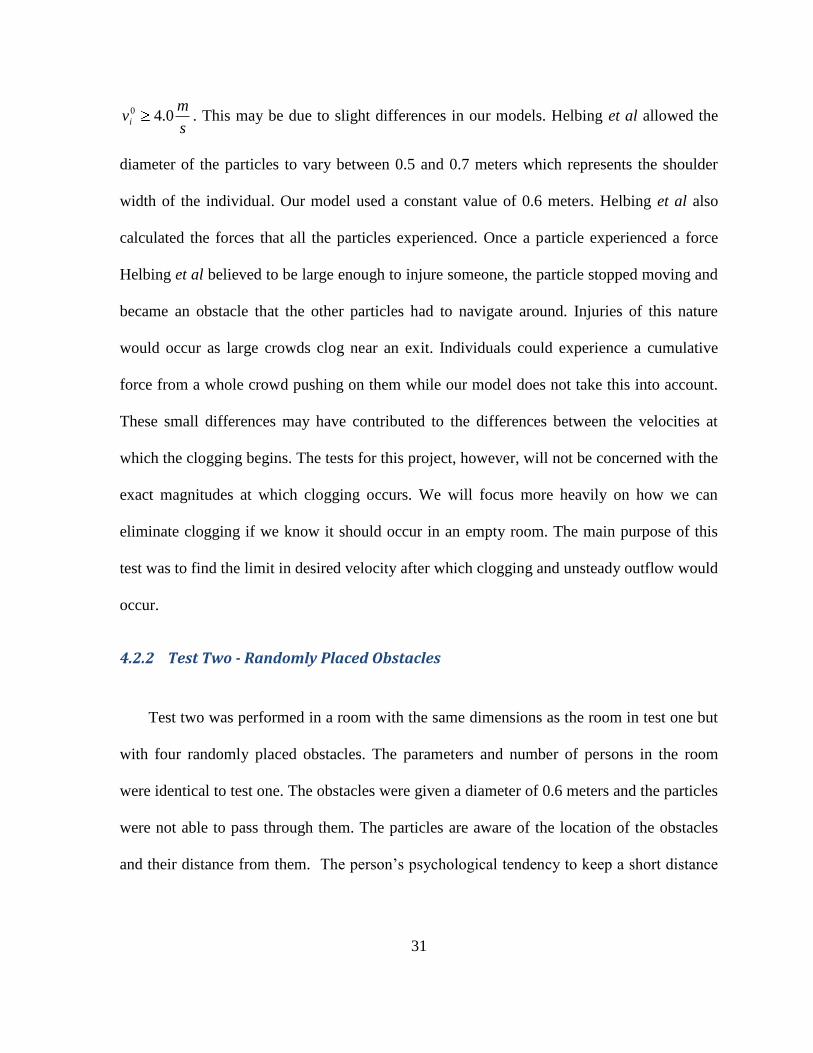
4.2.2 Test Two - Randomly Placed Obstacles

Test two was performed in a room with the same dimensions as the room in test one but

with four randomly placed obstacles. The parameters and number of persons in the room

were identical to test one. The obstacles were given a diameter of 0.6 meters and the particles

were not able to pass through them. The particles are aware of the location of the obstacles

and their distance from them. The person‟s psychological tendency to keep a short distance

32

from the obstacles is governed by the same equations as those for the walls and interactions

with one another.

0 2 4 6 8 100

1

2

3

4

5

6

7

8

9

10

Figure 13 - Distance Function Contour Plot with 4 Obstacles

Figure 13 shows a contour plot of the distance functions calculated from the walls and the

objects in the room for one configuration that was tested. The cooler colors represent a nearer

distance to the obstacles and walls and the warm colors represent a longer distance.

We ran this test with three different desired velocities as was done in test one with the

expectation for increased clogging and blockages once s

mvi 0.50 . In contrast to the findings

of test one, this clogging never occurred. The outflow remained relatively constant as can be

seen in Figure 14. A reasonable assumption, before running the test, would be that the

obstacles would slow the exit rate since the path to the door would now be obstructed for

33

many of the particles. When s

mvi 0.50 twenty-three people were able to escape with four

randomly placed objects in the room, the same end result as test one when ran with the same

desired velocity.

Figure 14 – Number of People That Have Exited Versus Time with Four Obstacles, 5 m/s Desired

Velocity

To show these results quantitatively we can define a clogging factor,

2

piTC where is the average time of escape per person and piT is the time of

exit of each person i . With the observation that clogging results in successive bursts of

people through the doorway separated by relatively long periods with no outflow at all, this

clogging factor will give an indication of how much clogging occurs relative to other tests.

Perfectly constant outflow would result in a clogging factor of zero and would increase as

clogging increased. The clogging factor for this test is approximately 1.68. Compared to the

34

clogging factor of approximately 3.46 from test one with s

mvi 0.50 the room with a small

number of scattered obstacles seems to be more desirable for less clogging. The obstacles

result in a 48% decrease in the clogging factor.

There could be many factors attributed to the decrease in clogging from test one to test

two. The placement of obstacles allowed the people to reach the doorway at different times.

Some people had no obstacles in their path and reached the doorway first. These people

would pass through the doorway with minimal clogging since there were very few of them.

People with an obstacle between them and the door had to navigate around it causing them to

arrive at the door later. With obstacles spaced out in a room with varying distances and

directions from the doorway, provided the people are scattered about the room randomly, the

times at which each person reaches the door could be significantly different. With the room

open and free of obstructions the people reached the doorway relatively quicker and all near

the same time.

Part of the success of this simulation seems to depend on the people being randomly

distributed throughout the entire room. Many people had to navigate around the obstacles

before flowing towards the doorway allowing those closest to it to pass through first with

minimal clogging. However, placing the people in one specific area of the room still

produced some clogging at the doorway. The test was most successful when many people

had to navigate around many different obstacles. When the particles were all congregated in

one area and had to navigate mostly around only one obstacle clogging still occurred. This

problem can be alleviated, however, if the obstacles are sufficiently close to the doorway as

will be shown in test three.

35

Despite the fact that test one and test two had the same number of people leave the room,

test two would seem to be the favorable one. The clogging experienced in test one could have

caused extreme pressures on the people nearest the doorway as all the people behind them

pushed forward. This could cause injuries and the people could have been immobilized. This

could decrease the outflow considerably as the injured people would turn into obstacles

themselves. Had the crowd of people been running away from a fire, this could cause the fire

to reach the people in the back of the crowd before they could leave the room resulting in

more potential injuries or deaths.

4.2.3 Test Three- Line of Objects in center of the room.

For the next test we placed three objects in a straight line in the center of, and

perpendicular to, the doorway which essentially separated the room into two sections. The

main purpose of this was to analyze how objects placed close to the door would affect the

outflow.

0 2 4 6 8 100

1

2

3

4

5

6

7

8

9

10

Figure 15 - Distance function contour plot with 3 objects

36

Figure 15 shows the placement of the three obstacles in the room and the distance function

calculated around them and the walls. The parameters and number of people were kept the

same as tests one and two. Twenty people were scattered randomly on each side of the three

obstacles.

This test showed minimal signs of clogging fors

mvi 0.50 . The particles to the left

and right of the line of obstacles stayed on their respective sides without moving between the

objects. The line of objects forced two separate lanes of particles to flow through the

doorway if the distance from the doorway to the closest obstacle was sufficiently small

enough to not allow clogging. This caused steady outflow and allowed two more people to

pass through the doorway than the previous tests withs

mvi 0.50 .

This configuration was tested first with the center of the obstacle closest to the

doorway set 1.5 meters back from it as is shown in Figure 15. Setting the desired velocity

s

mvi 0.50

this configuration resulted in a clogging factor of approximately 1.48, a 12%

decrease from test two and a 58% decrease from test one both with the same desired velocity.

This test allowed two more people to pass through the doorway than that of test one and two

suggesting this is the most desirable of the three tests for maximum outflow.

Since the obstacle closest to the doorway was the only obstacle directly responsible

for separating the crowd into two lanes we decided to run the simulation with the two

37

obstacles farthest from the doorway removed leaving only the one closest one to the doorway

as shown in Figure 16.

0 2 4 6 8 100

1

2

3

4

5

6

7

8

9

10

Figure 16 - Distance function contour plot with 1 object

This configuration allowed one more person to leave the room than the configuration in

Figure 15 while the clogging factor was negligible. This could be due to the additional

friction effects the people experience from three obstacles relative to one slowing their

velocity and not allowing them to reach the door as quickly. Since the obstacle closest to the

door is the only obstacles eliminating clogging the additional two obstacles seem

unnecessary.

This test demonstrates the most desirable of the three room configurations we tested. As

opposed to test two, this configuration guarantees to eliminate clogging regardless of the

placement of people throughout the room. The distance between the doorway and the closest

obstacle was too small to allow a buildup of people. Placing the center of the obstacle in line

with the center of the doorway is necessary to allow an even flow of people on each side.

38

Placing the center of the obstacle 1 meter from the doorway seemed to allow the greatest

outflow. With the diameter of the obstacle and the person both being 0.6 meters this allowed

only 0.1 meters of free space on each side of a person as it passed between the doorway and

the obstacle. This small amount of space made it impossible for more than one person to pass

each side of the obstacle

39

5 Recommendations and Conclusions

Due to the nature of the Major Qualifying Project and the brevity of the allotted time to

its creation, there are many further avenues that can be explored with regards to this project.

The following sections explain our recommendations for future actions that can be taken to

improve upon our project. Although we feel we met our goals, we believe that there are many

more avenues that can be explored.

5.1 The Decision Rule

This project‟s target objective was to write a program that could predict the movements

of individuals within a crowd by modeling them after particles. Each particle followed a list

of equations based on Newton‟s Second Law of Motion. Each particle followed the same set

of rules, without regard to individuality. However, as is simple to understand, in a real crowd

of people, the individuals that make up the crowd are anything but homogeneous. That is to

say, everything from the individual‟s physical characteristics to their mental mindsets can be

very dissimilar to the other individuals within the crowd. This project, therefore, lacks what

seems to be a very important feature; the various characteristic differences between the

individuals with a crowd.

To investigate the different individual characteristics that could be contributed to the

particles we turned to a few sources. The first was a 1988 (4)

study of human collective

dynamics. The study involved developing a mathematical model involving two adversarial

groups. The individuals within the groups were given a set of equations that dictated their

goals and objectives and controlled their effectiveness in reaching their targets. If their goal

40

alone was applied to this project, we could formulate equations that would control the rate of

success of the individuals within our model.

The authors of this 1988 study recognized that a complete model would require every

particle to have its own set of parameters that dictate its movement. However, individualizing

each particle would making the setup very complex so they decided to choose, what they

believed to be, the more important characteristic parameters and apply them to all of the

particles. The following is a list of the characteristics they selected:

1. The position of the individual

2. The velocity of the individual

3. The individual‟s level of excitement

4. The individual‟s level of fear

5. The individual‟s level of anger

6. The individual‟s response to peer influence

7. The individual‟s sense of moral obligation

8. The individual‟s ability to communicate

9. The individual‟s health

After selecting the important characteristics, the authors assigned variables that would

control each of the characteristics. For example, the individual‟s level of excitement is

related to seeing enemy casualties and visible team success, where the individual‟s level of

fear is related to seeing comrade casualties, team failure, enemy excitement, comrade panic,

and lose of ammo.

41

The second source that we turned to in order to better understand which

characteristics we could recommend was with Professor Jim Doyle. A Social Science and

Policy Studies Professor at Worcester Polytechnic, Professor Doyle offered some great

insight into the world of human behavior. He suggested each particle be given a decision

rule; a set of variables that would allow for individual characteristics between the members

within the crowd. For example, adding a level of bravery to various individuals may give a

sense of compassion to the particles so that they may help a slower particle along. Another

characteristic could be the desire to move toward the nearest exit, rather than the one that the

majority of the crowd is flocking to. Professor Doyle also recommended a time delay within

the crowd. This would simulate a more realistic event in that not everyone is knowledgeable

of the life-threatening situation at the same instance, as is the case with our program.

We feel that these few subtle changes are essential to get a more accurate

understanding of the motions of individuals within a crowd. Although our project gives a

basic depiction of the movements of individuals with regard to forces between themselves

and the walls, there are obviously other factors at play with regard to the human psyche.

5.2 Future Tests

Although our project has expanded upon the Helbing et al model by adding obstacles for

the particles to avoid, there are still many other situations that can be examined. Our model is

relatively simple with regard to the complexity real-life room geometries and human

interactions. This section will discuss a few ideas that can be explored for future MQP‟s that

may follow this project.

42

Beginning work with a program and code that is already functional would allow more

time to be devoted to testing and other analysis. We found that due to the learning curve

involved with understanding the computer programs used to create our code, we were limited

in the amount of exploration we could achieve due to the time constraints.

Our model, although seemingly accurate at mimicking the motion of crowds, is quite

simple. In our model there are a limited number of people in the confined space and everyone

is attempting to move in the same direction. In most situations there are many more people

involved in a situation than we tested and not everyone has the same immediate desires.

Many people may know of more than one exit and have to make a decision which one to

choose. Psychological tendencies for people to do as others around them do could be

examined and incorporated into the model.

By adding more people to the room, more of the computer‟s resources are used up

and the testing length is increased. Future tests could take into account larger rooms more

people. Rooms similar to the configurations of stadiums with thousands of people and

multiple exits could be simulated.

Our simulated room is rectangular, although this is a simulation of many real world

environments such as a small office. Many rooms have much more complex geometries that

could affect the results of the tests. We recommend that more complex geometries be tested

that may simulate a curving hallways or a stairway so that more realistic simulations can by

observed. Different sizes and shapes of obstacles could be taken into account. Since our

model was concerned more with the placement of obstacles we did not take into account

different sizes or shapes.

43

We were able to recreate the model by Helbing et al by studying his work. He has used

his model to investigate how to increase the flow of individuals from an area but there can

still be more done. We recommend that our model be used to look into possible scenarios in

assist with crowd control and exit flow. By placing different size and shaped objects in the

confined space and moving them to different locations, patterns can be observed that could

lead to a better knowledge of how crowds function.

44

6 Works Cited

1. Helbing, D. & Mulnar, P. “Social force model for pedestrian dynamics”. Phys. Rev. E

51, 4284-4286 (1995).

2. Helbing, D., Farkas, I., and Vicsek, T. “Simulating Dynamical Features of Escape

Panic.” NATURE 407 (2000): 487-490.

3. Hughes, R.. L. “The Flow of Human Crowds.” Annual Reviews of Fluid Mechanics

35 (2003): 169-183.

4. Genin, K. E., Harlow, F. H., and Scandoval, D. L.“Human Collective Dynamics: Two

Groups in Adversarial Encounter”. National Technical Information Service. Los

Alamos National Lab, 1988.

5. Predtetschenski, W.M. & Milinski, A.I. Personenströme in Geäuden-

Berechnungsmethoden für die projektierung (Müller, Köln-Braunsfeld, 1971).

6. Quarantelli, E L., Panic Behavior: Some Empirical Observations. 19 July 1975.

< http://dspace.udel.edu:8080/dspace/handle/19716/393>

7. Quarantelli, E L. “The Nature and Conditions of Panic.” American Journal of

Sociology (1954): 267-275. 2 Feb. 2008

<http://www.jstor.org/view/00029602/dm992497/99p0794w/0>.

8. Still, K. G. Crowd Dynamics. Aug. 2000. 29 Jan. 2008

<www.crowddynamics.com/Thesis/Chapter%202.htm>.

9. Unterstell, R. “The Dynamic of Panic.” German Research (2006): 21-23.

45

7 Appendix A- The Code

clear; clc; close all;

mx=45; my=45;

d=zeros(mx,my); dx=zeros(mx,my); dy=zeros(mx,my);

Lx=10;Ly=10;

hx=Lx/(mx-1); hy=Ly/(my-1);

x=0:Lx/(mx-1):Lx; y=0:Ly/(my-1):Ly;

N_Obst=X; xx=[X]; yy=[X]; rr=[X];

d(1:mx, 1:my)=Lx+Ly;

for i=1:1:mx

x(i)=(i-1)*hx;

for j=1:1:my

y(j)=(j-1)*hy;

for n=1:1:N_Obst

dtemp=sqrt((xx(n)-x(i))^2+(yy(n)-y(j))^2)-rr(n);

if dtemp<d(i,j); d(i,j)=dtemp; end

end

dtemp=sqrt((x(i)-0.5*Lx)^2+(y(j)-0.45*Ly)^2);if dtemp<d(i,j); d(i,j)=dtemp; end

dtemp=sqrt((x(i)-0.5*Lx)^2+(y(j)-0.55*Ly)^2);if dtemp<d(i,j); d(i,j)=dtemp; end

if(y(j) <0.45*Ly), dtemp=sqrt((0.5*Lx-x(i))^2); if dtemp<d(i,j); d(i,j)=dtemp; end

elseif (y(j) > 0.55*Ly), dtemp=sqrt((0.5*Lx-x(i))^2); if dtemp<d(i,j); d(i,j)=dtemp;

end

end

dtemp=sqrt((Ly-y(j))^2); if dtemp<d(i,j); d(i,j)=dtemp; end

dtemp=sqrt((0-y(j))^2); if dtemp<d(i,j); d(i,j)=dtemp; end

dtemp=sqrt((0-x(i))^2); if dtemp<d(i,j); d(i,j)=dtemp; end

end

end

for i=2:1:mx-1

for j=2:1:my-1

dx(i,j)=(d(i+1,j)-d(i-1,j))/(2*hx);

dy(i,j)=(d(i,j+1)-d(i,j-1))/(2*hy);

end

end

k=1.2*10^5; kap=2.4*10^5;

Ai=2*10^3; Bi=0.08;

mass=80; tau=0.5;

dt=0.0025;

endtime=15;

n=X;

up=zeros(1,n); vp=zeros(1,n);ugiven=zeros(1,n); vgiven=zeros(1,n);

xp=zeros(1,n); yp=zeros(1,n);

xp=[X];

yp=[X];

up=0*[X];

vp=[X];

ugiven=0*[X];

vgiven=[X];

rp(1:n)=0.3;

t=0:dt:endtime;

time(1)=0.0;esc(1)=0;

46

for p=1:length(t);

for l=1:n;

xold=xp(l); yold=yp(l); uold=up(l); vold=vp(l);

fx=0; fy=0;

ip=floor((xp(l)/Lx)*mx)+1; jp=floor((yp(l)/Ly)*my)+1;

ALx=(xp(l)-hx*(ip-1))/hx; ARx=1.0-ALx;

ALy=(yp(l)-hy*(jp-1))/hy; ARy=1.0-ALy;

A1=ALx*ALy; A2=ARx*ALy; A3=ARx*ARy; A4=ALx*ARy;

dwx=A1*(dx(ip+1,jp+1))+A2*(dx(ip,jp+1))+A3*(dx(ip,jp))+A4*(dx(ip+1,jp));

dwy=A1*(dy(ip+1,jp+1))+A2*(dy(ip,jp+1))+A3*(dy(ip,jp))+A4*(dy(ip+1,jp));

dw=A1*(d(ip+1,jp+1))+A2*(d(ip,jp+1))+A3*(d(ip,jp))+A4*(d(ip+1,jp));

for m=1:n;

if l~=m;

dxp=xp(l)-xp(m); dyp=yp(l)-yp(m);

dup=up(m)-up(l); dvp=vp(m)-vp(l);

dij=sqrt(dxp^2+dyp^2);

nx=dxp/dij; ny=dyp/dij;

tx=-ny; ty=nx;

tangVel=dup*tx+dvp*ty;

g=0.0; if (rp(l)+rp(m)>dij); g=1.0;end;

fx=fx+(Ai*exp((rp(l)+rp(m)-dij)/Bi)+k*g*(rp(l)+rp(m)-dij))*nx+...

kap*g*(rp(l)+rp(m)-dij)*tangVel*tx;

fy=fy+(Ai*exp((rp(l)+rp(m)-dij)/Bi)+k*g*(rp(l)+rp(m)-dij))*ny+...

kap*g*(rp(l)+rp(m)-dij)*tangVel*ty;

end

end

g=0.0; if(rp(l)>dw),g=1.0;end;

twx=dwy;twy=-dwx;

tangVel=up(l)*twx+vp(l)*twy;

fx=fx+(Ai*exp((rp(l)-dw)/Bi)+k*g*(rp(l)-dw))*dwx-kap*g*(rp(l)-dw)*tangVel*twx;

fy=fy+(Ai*exp((rp(l)-dw)/Bi)+k*g*(rp(l)-dw))*dwy-kap*g*(rp(l)-dw)*tangVel*twy;

xp(l)=xold+dt*uold;

yp(l)=yold+dt*vold;

ugiven(l)=(0.5*Lx-xp(l));vgiven(l)=(0.5*Ly-yp(l));vv=sqrt(ugiven(l)^2+vgiven(l)^2);

ugiven(l)=5*ugiven(l)/vv; vgiven(l)=5*vgiven(l)/vv;

if(xp(l)>0.475*Lx),ugiven(l)=0.5; vgiven(l)=0.0;end

up(l)=uold+dt*((ugiven(l)-uold)/tau+fx/mass);

vp(l)=vold+dt*((vgiven(l)-vold)/tau+fy/mass);

if(xp(l)>Lx-hx), xp(l)=xold;yp(l)=yold;up(l)=0;vp(l)=0;end

xxp(p,l)=xp(l); yyp(p,l)=yp(l);

end

hold off;[xx,yy,zz]=cylinder(0.3); xx=xx+xp(1);

yy=yy+yp(1);surf(xx,yy,zz);axis([0,Lx,0,Ly,0,3]);

hold on;

plot([0.5*Lx,0.5*Lx],[0.0,0.45*Ly],'LineWidth',3);

plot([0.5*Lx,0.5*Lx],[0.55*Ly,Ly],'LineWidth',3);

for l=2:n;[xx,yy,zz]=cylinder(0.3); xx=xx+xp(l);yy=yy+yp(l);surf(xx,yy,zz);hold on;end

pause(0.01)

esc(p+1)=0;

for l=1:n;

if(xp(l)>5),esc(p+1)=esc(p+1)+1;end

end

time(p+1)=time(p)+dt;

end

47

figure

plot(time,esc);

figure

plot(xxp(:,1),yyp(:,1), '-*b');hold on,

plot([0.5*Lx,0.5*Lx],[0.0,0.45*Ly],'LineWidth',3);plot([0.5*Lx,0.5*Lx],[0.55*Ly,Ly],'LineWidt

h',3);

contour(x,y,rot90(fliplr(d)),50);

contour(x,y,rot90(fliplr(d)),[0 0],'linewidth',4); axis([0 Lx 0 Ly]);axis square