Modeling the Yield Curve

Bob StineStatistics Department, Wharton

Choong Tze Chua, Singapore Mgmt UnivKrishna Ramaswamy, Finance Department

Plan for TalkBackgroundWhat is the yield curve?What makes it interesting and important?ExamplesCashCommodities (primarily crude oil)

Data analysis is simpler with pricesHow to recognize arbitrage?More natural structure

Commodities are differentLinkages among products

2

Background

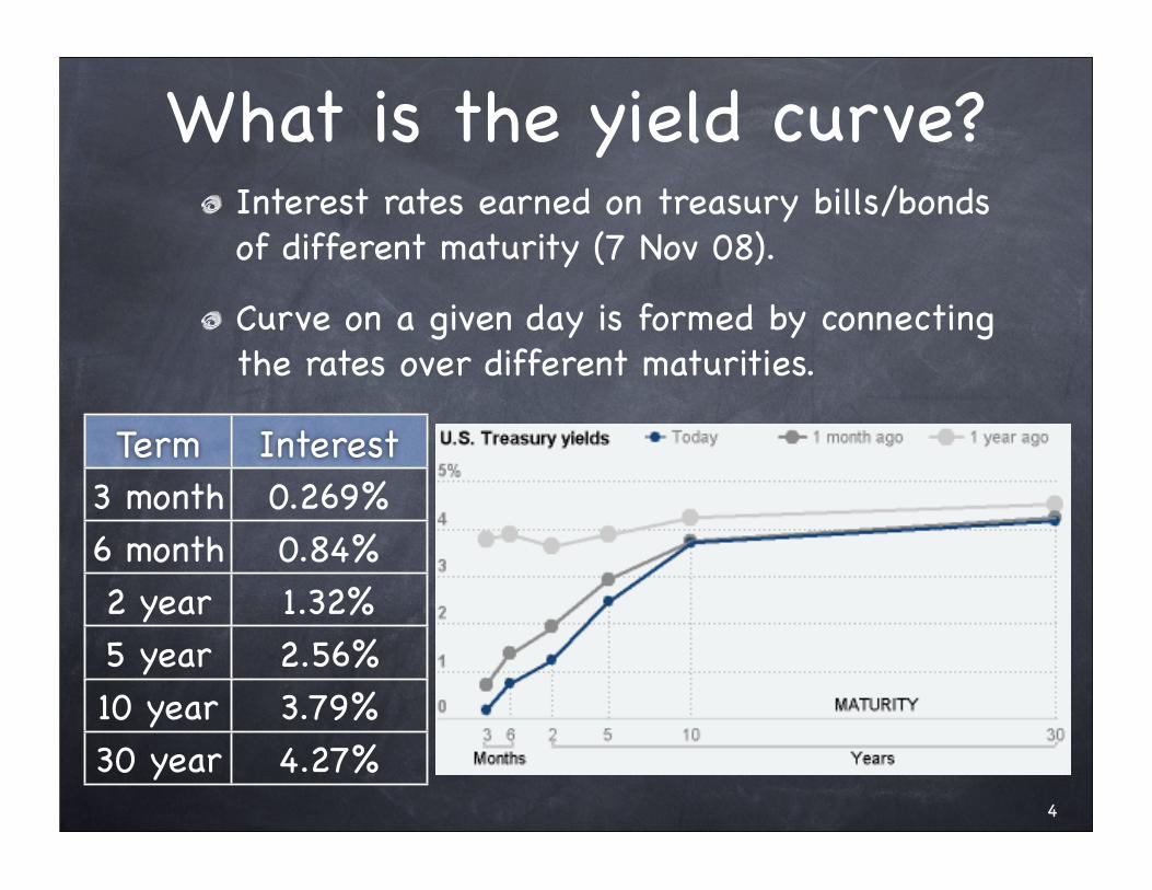
What is the yield curve?Interest rates earned on treasury bills/bonds of different maturity (7 Nov 08).

Curve on a given day is formed by connecting the rates over different maturities.

4

Term Interest3 month 0.269%6 month 0.84%2 year 1.32%5 year 2.56%10 year 3.79%30 year 4.27%

What is the yield curve?Interest rates derived from contracts in the Eurodollar option market.London Interbank Offered Rate (LIBOR)Interest rate on a 3-month contract in the futurePlot shows instantaneous forward rates.

52 4 6 8 10

!

3.0

3.5

4.0

4.5

5.0

5.5

"2008.16

Many more

contracts

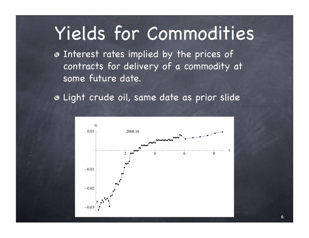
Yields for CommoditiesInterest rates implied by the prices of contracts for delivery of a commodity at some future date.

Light crude oil, same date as prior slide

6

2 4 6 8!

"0.03

"0.02

"0.01

0.01#

2008.16

QuestionsWhat are the dynamics of the yield curve?

How fast does it change? Can you predict where it’s headed?

How is the yield for cash related to yields implied by commodities that include convenience factors?

How are yields for various products related to one another?

What’s the connection between these “curves” and the underlying data?

7

Dynamics

Plots: CashYields on cash over period of about 100 daysRed curve is the originalGray curves are separated by 10 trading days

Some changes are large, other curves cluster together

92 4 6 8 10

!

3.0

3.5

4.0

4.5

5.0

5.5

6.0

"

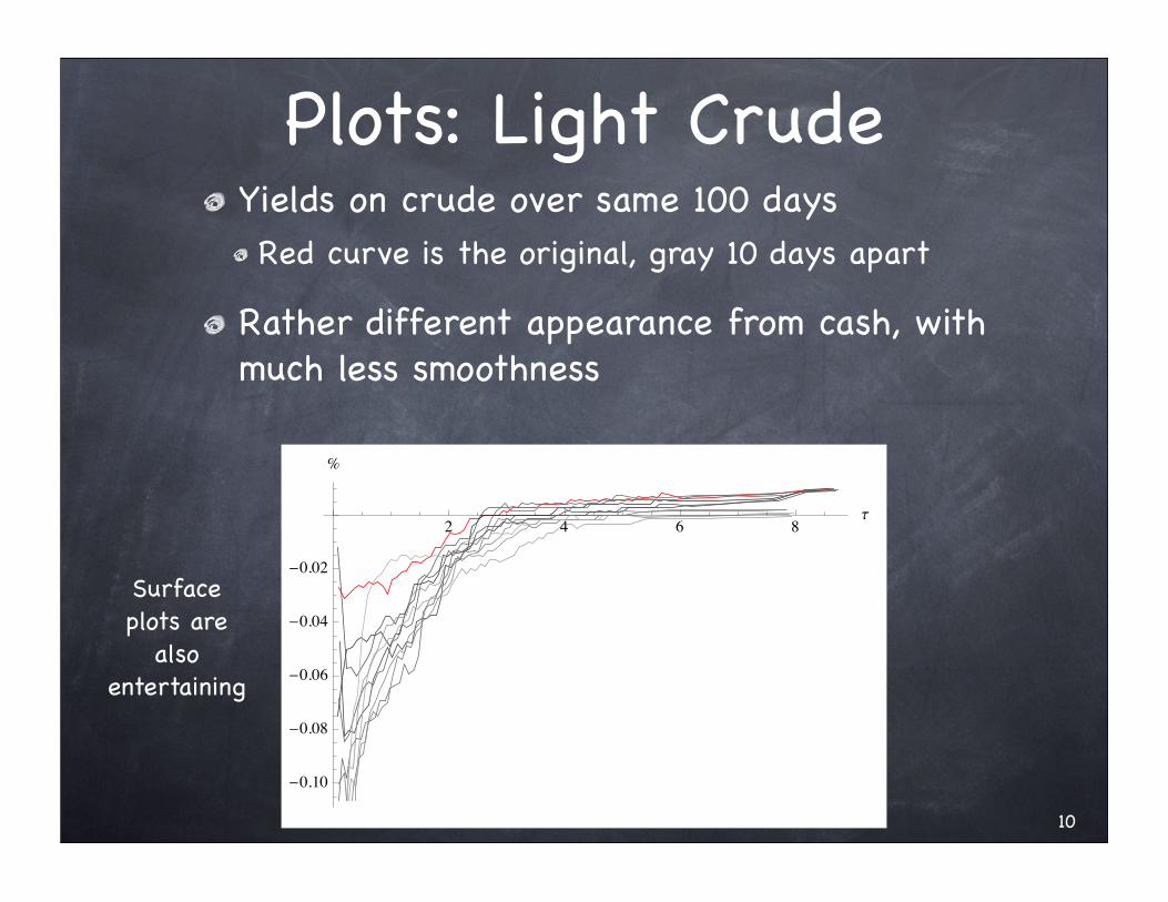
Plots: Light CrudeYields on crude over same 100 daysRed curve is the original, gray 10 days apart

Rather different appearance from cash, with much less smoothness

10

2 4 6 8!

"0.10

"0.08

"0.06

"0.04

"0.02

#

Surface plots are

also entertaining

Relations Among ProductsDependent movements over 10-day intervals for heating oil and light crude.Strong seasonal pattern for heating oil that is not apparent in yield on light crude.

0.4 0.6 0.8 1.0 1.2!

"0.2

"0.1

0.1

0.2

#

HO

CL11

ModelsModels provide parsimonious way to predict where the curve is heading.Rather than have to predict a “curve”, forecast the value of certain parameters in a regression-like formula for the curve

Model used resembles a polynomial, but on a logarithmic scale more suited to description of rates.

Modeling issues (see paper)How many polynomial terms?Does the model allow arbitrage?

12

DecompositionDecompose the yield curve yt(τ) into three components! ! ! yt(τ) = U(τ) + Mt(τ) + Dt(τ)

Long-term unconditional expectation! ! ! ! ! ! Es ys(τ) = U(τ)

Other terms are separable in τ and t, factoring as Mt(τ) = mt g(τ)

Maturity specific component is mean revertingm(t) follows log normal SDE with expectation! ! ! ! ! Es mt = ms e-k(t-s) s<t

13

Decomposition, cntdDate specific term is also mean reverting, but captures effects that move toward origin with time! ! ! ! Es Dt(τ) = Ds(τ+t-s) s<t,τEach contract carries the date-specific effect

If dt follows log normal SDE, then h(τ) = e-kτ

! ! Es Dt(τ) = (ds e-k(t-s)) e-kτ = Ds(τ+t-s)

Example (2,2,3)2nd order unconditional curve2 maturity-specific functions ! ! mt,1 = cm1 (e-kτ - e-2kτ) , mt,2 = cm2 (e-kτ - e-4kτ)3 date-specific functions

14

Component FunctionsBasis elements for expressing a model for the yield curve using component SDEs

Constant k determines shapes

0.5 1.0 1.5 2.0 2.5 3.0

0.1

0.2

0.3

0.5 1.0 1.5 2.0 2.5 3.0

0.2

0.4

0.6

0.8

1.0

Mt(τ) Dt(τ)

15

Fitted Yield CurvesExtracted state coefficients for several daysEstimates are smoother than those for each dayUnconditional, maturity, date components‣Observation error ought to be uncorrelated

1 2 3 4!

"0.2

"0.1

0.0

0.1

0.2

0.3

0.4

0.5#

2006.87

16

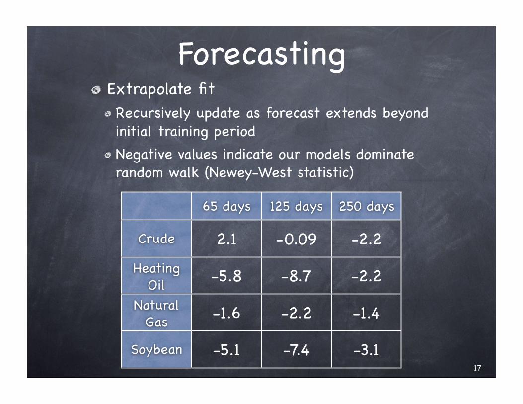
ForecastingExtrapolate fitRecursively update as forecast extends beyond initial training periodNegative values indicate our models dominate random walk (Newey-West statistic)

65 days 125 days 250 days

Crude

Heating Oil

Natural Gas

Soybean

2.1 -0.09 -2.2

-5.8 -8.7 -2.2

-1.6 -2.2 -1.4

-5.1 -7.4 -3.117

Data

Never underestimate the time that it takes to prepare the data.

PricesYields are not directly observedObtain prices of futures contracts from data vendor CRB TraderPrices are much smoother

19

2 4 6 8!

"0.03

"0.02

"0.01

0.01#

2008.16

2 4 6 8!

88

89

90

91$

2008.16

From Price to YieldCompute the yield at the midpoint between two observed prices as the continuously compounded rate of interest! ! ! ! ! ! log pt(τ+d) - log pt(τ)! !! ! yt(τ) = ! ! ! ! ! ! ! ! ! ! ! as d -> 0

ResultsDifferencing magnifies random noiseObserved only at discrete set of pointsTerminal date is about 15 daysNo observed spot rateAnomalies (aka, “market microstructure”)

20

d

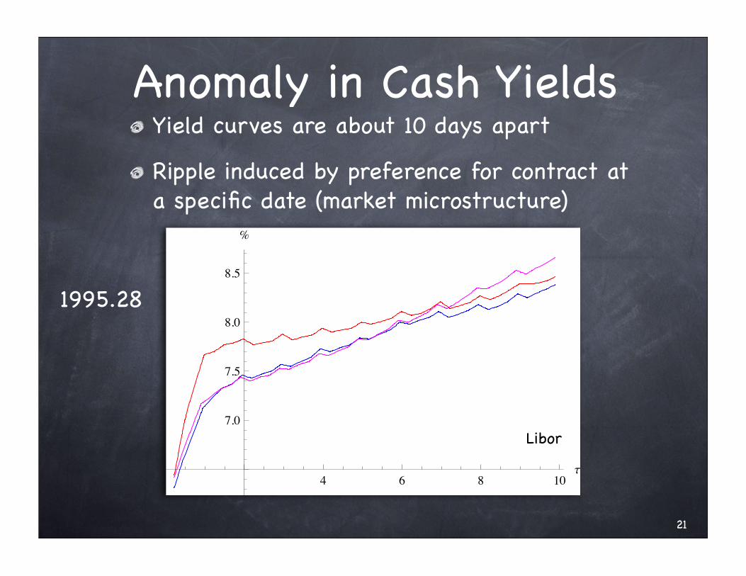
Anomaly in Cash YieldsYield curves are about 10 days apart

Ripple induced by preference for contract at a specific date (market microstructure)

1995.28

4 6 8 10!

7.0

7.5

8.0

8.5

"

Libor

21

Anomaly: Sticky PriceA contract for light crude did not trade this day, so price stayed same as on prior day

Rest of the curve shifted

22

1 2 3 4 5 6!

"0.10

"0.05

0.05#

1999.35

1 2 3 4 5 6!

16.0

16.2

16.4

16.6

16.8

17.0

17.2$

1999.35

Patching AnomaliesAdaptive procedure that will not introduce side effects

Approach is to follow a contract over time rather than fixed maturityAvoid interpolation-induced transitionsContracts have a more consistent sequential pattern than in yields over varying maturities

Contracts follow a diagonal in the data! ! ! yt(τ)! ! for fixed expiry date t+τ

t

τ

23

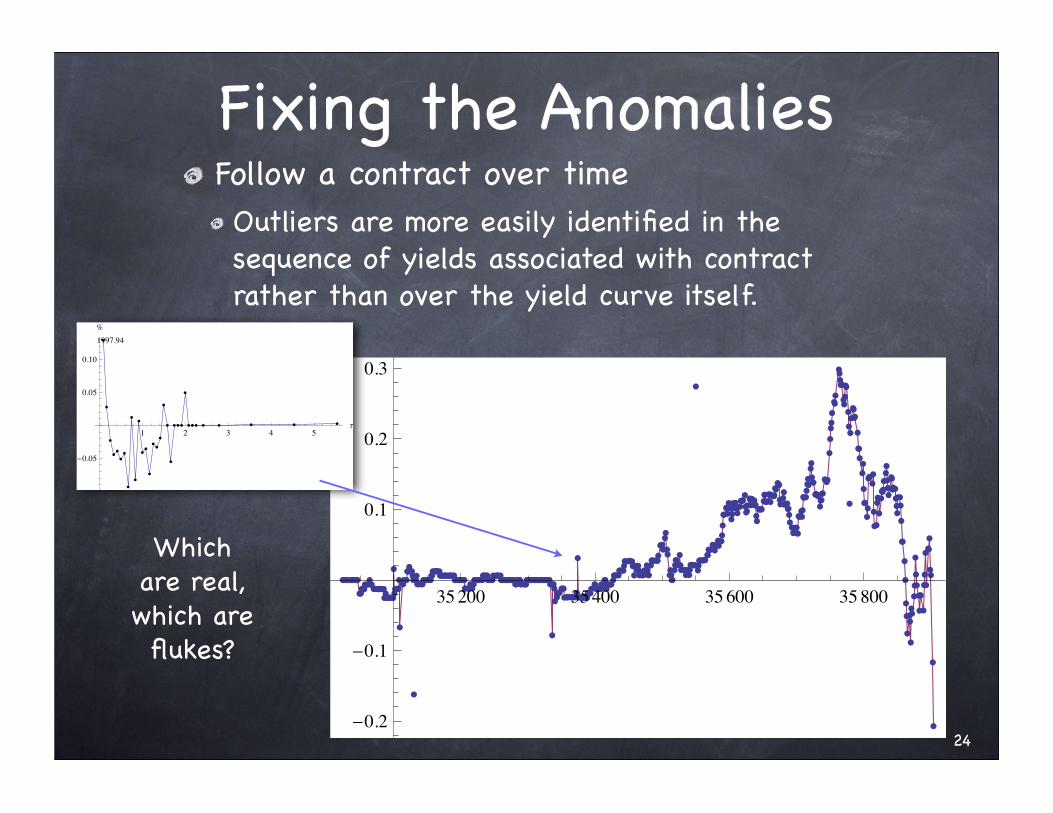
Fixing the AnomaliesFollow a contract over timeOutliers are more easily identified in the sequence of yields associated with contract rather than over the yield curve itself.

35200 35400 35600 35800

!0.2

!0.1

0.1

0.2

0.3

1 2 3 4 5!

"0.05

0.05

0.10

#

1997.94

24

Which are real, which are flukes?

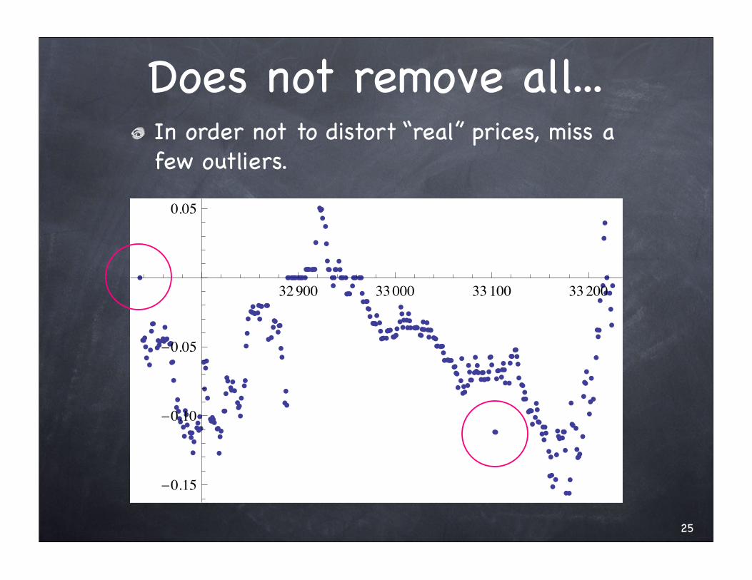
Does not remove all...In order not to distort “real” prices, miss a few outliers.

32900 33000 33100 33200

!0.15

!0.10

!0.05

0.05

25

Nor a sustained problem...Moving medians of length 3 cannot patch a period with a sustained anomaly.

35600 35800 36000 36200 36400

!1.5

!1.0

!0.5

1 2 3 4 5

!0.10

!0.05

0.05

0.10

0.15

0.20

0.25

persists for about 3 weeks26

Contracts

Time Series ModelsStructural modelDescribes the yield curve as a function f(τ)Can evaluate f(τ) at any maturityTheoretical properties, derived quantities

Time seriesConsiderable methodology availableCannot hold maturity τ fixed unless were able to observe yt(τ) for all tInterpolation between points introduces artifacts

Following a single contract provides most direct series

28

Yields of ContractsThink of data as collection of contracts yt(τ) identified by expiry dateContracts end, becoming more variable as τ approaches 0 where yield is more volatile.

0 100 200 300 400 500 600

−0.1

0.0

0.1

0.2

0.3

0.4

Day 35694

Rows from Expiration

Rate

29

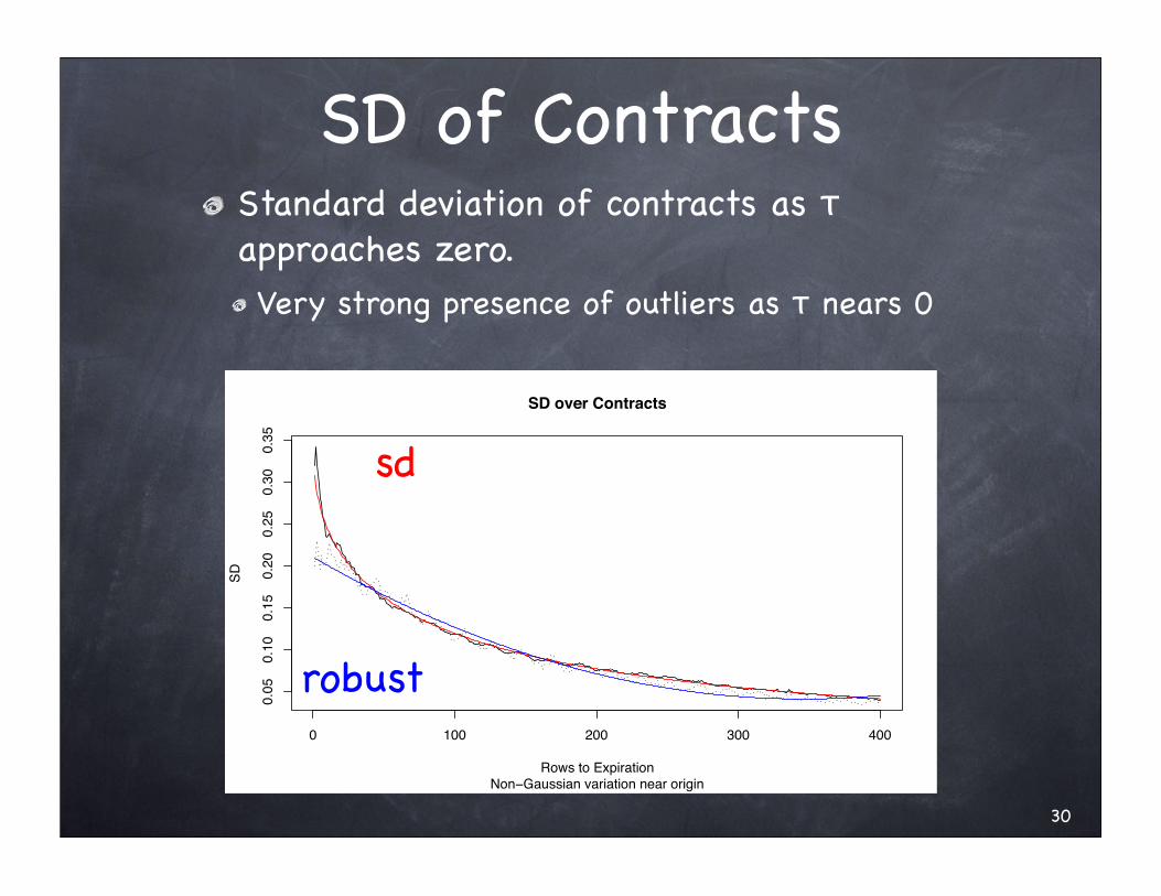
SD of ContractsStandard deviation of contracts as τ approaches zero.Very strong presence of outliers as τ nears 0

0 100 200 300 400

0.05

0.10

0.15

0.20

0.25

0.30

0.35

SD over Contracts

Non−Gaussian variation near originRows to Expiration

SD

sd

robust

30

CointegrationDifferences in yields of adjacent contracts are non-stationary as time gap increases

Suggests that contracts are cointegrated when not “too far” apartDegree of time separation also measures the rate of change in the yield curve, a sort of stochastic modulus of continuity of the yield Interpret the source of non-stationarity as due to movements of some underlying yield processLatent variable type of model

31

Prices of ContractsPrices again seem simpler to use

Plot shows prices of 4 contracts for light crude, about 100 days apart

3230400 30500 30600 30700 30 800 30900

26

27

28

29

30

31

mid 1984

Prices of ContractsPrices again seem simpler to use

Plot shows prices of 4 contracts for light crude, about 100 days apart

33

early 2007

38000 38 200 38400 38600 38800 39000 39200

60

80

100

120

More thingsMultivariate structureHow to use the evident contemporaneous movements in prices or yields for various products (such as the various soy commodities)Related to movements in yield for cash as well

Model after subtracting out the yield for cash to extract a convenience yieldImplications for stationarity after remove the yield: simpler model?

34

SummaryModels for yield curveCapture dynamics of yieldsDate and maturity specific decomposition relevant for commodities as wellOut-of-sample performance superior to random walk benchmark

Data analysis suggests reasons to work with contracts rather than a function to maturityOutliersMore amenable to statistical methods

Many unresolved questions

35