modeling uncertainty in integrated assessment of climate ...1 modeling uncertainty in integrated...
TRANSCRIPT

1
Modeling Uncertainty in Integrated Assessment of Climate Change:
A Multi-Model Comparison
By KENNETH GILLINGHAM, WILLIAM NORDHAUS, DAVID ANTHOFF, GEOFFREY BLANFORD,
VALENTINA BOSETTI, PETER CHRISTENSEN, HAEWON MCJEON, AND JOHN REILLY*
The economics of climate change involves a vast array of uncertainties, complicating
our understanding of climate change. This study explores uncertainty in baseline
trajectories using multiple integrated assessment models commonly used in climate
policy development. The study examines model and parametric uncertainties for
population, total factor productivity, and climate sensitivity. It estimates the
probability distributions of key output variables, including CO2 concentrations,
temperature, damages, and social cost of carbon (SCC). One key finding is that
parametric uncertainty is more important than uncertainty in model structure. Our
resulting distributions provide a useful input into climate policy discussions.
* Corresponding Authors: Kenneth Gillingham and William Nordhaus. Gillingham: Yale University, 195 Prospect Street New Haven, CT 06511
([email protected]); Nordhaus: Yale University, 28 Hillhouse Avenue, New Haven, CT 06511 ([email protected]); Anthoff:
UC Berkeley; Blanford: Electric Power Research Institute; Bosetti: Bocconi University; Christensen: University of Illinois Urbana-Champaign;
McJeon: Joint Global Change Research Institute; Reilly: MIT. The authors are grateful for comments from many colleagues over the course of this
project. These include individual scholars as well as those at seminars and workshops at Yale University, the University of California, Berkeley, and
the Snowmass climate-change meetings organized under the aegis of the Energy Modeling Forum. The authors are grateful to the Department of
Energy and the National Science Foundation for primary support of the project. Reilly and McJeon acknowledge support by the U.S. Department of
Energy, Office of Science. Reilly also acknowledges the other sponsors the MIT Joint Program on the Science and Policy of Global Change listed at
http://globalchange.mit.edu/sponsors/all. Bosetti acknowledges funding from the European Research Council 336703 – project RISICO. The Stanford
Energy Modeling Forum has provided support through its Snowmass summer workshops.

2
I. Introduction
A central issue in the economics of climate change is understanding the vast array of uncertainties
and synthesizing them in a way useful to policymakers. These uncertainties range from those
regarding economic and population growth, emissions intensities and new technologies, to the
carbon cycle, climate response, and damages, and cascade to the costs and benefits of different
policy objectives.
This study examines uncertainty in baseline trajectories in major outcomes for climate change
using multiple integrated assessment models (IAMs), with a goal of quantifying how uncertainty
propagates through the economic and climate models and what this implies for outcomes critical to
climate policy development. The six well-known models used in the study are representative of the
models used in the IPCC Fifth Assessment Report (IPCC 2014) and in the U.S. government
Interagency Working Group Report on the Social Cost of Carbon or SCC (US Interagency Working
Group 2013). We focus our efforts in this study on three key uncertain parameters: population
growth, total factor productivity growth, and equilibrium climate sensitivity. For the estimated
uncertainty in these three parameters, we develop estimates of the uncertainty to 2100 for major
output variables, such as emissions, concentrations, temperature, per capita consumption, output,
damages, and the SCC. These variables are of direct interest to policymakers concerned about the
design of emissions-reducing policies that have a starting point near a baseline trajectory (one with
very limited climate policies). Understanding uncertainty in baseline trajectories is a critical part of
climate change research regardless of the likelihood of future policy intervention (although it is
worth noting that we have been close to a baseline trajectory in the recent past). Baseline
trajectories determine the scale of the future economic system, a fundamental input in the
calculation of the benefits and costs associated with climate change policies, including both market
and non-market damages and the costs of emissions mitigation efforts. Further, the baseline
trajectory is the path with the largest dispersion of outcomes. The most recent IPCC assessment
(IPCC 2014) identified a more formal understanding of uncertainty around baseline projections in
particular as a key research need.
Our study develops a new two-track approach that permits reliable quantification of uncertainty
for models of greatly differing size and complexity. The first track involves performing model runs
over a set of grid points and fitting a flexible numerical approximation (a surface response function)
to the results from each model; this approach provides a quick and accurate way to emulate running
the models. The second track develops probability density functions for the chosen input parameters

3
(i.e., the parameter pdfs) using the best available evidence. We then combine both tracks by
performing Monte Carlo simulations using the parameter pdfs and the surface response functions.
This approach provides a transparent, easy to communicate, easy to replicate, and most
importantly feasible approach for studying baseline uncertainty across multiple parameters and
models. Running the two tracks in parallel also permitted this study to be completed in a reasonable
timeframe. The approach can easily be applied to additional models and uncertain parameters. An
important aspect of the approach, unlike virtually all other inter-model comparison exercises, is its
replicability. The approach is easily validated because the data from the calibration exercises are
relatively compact and are compiled in a compatible format, the surface responses can be estimated
independently, and the Monte Carlo simulations can be easily run in multiple existing software
packages. Thus, a first major contribution of this paper is laying out an approach for quantifying
model uncertainty in baseline trajectories that can be readily applied to climate economics, as well
as to analyses such as those of the U.S. Interagency Working Group on the Social Cost of Carbon.
A second major contribution of this paper is substantive: it presents a set of distributions of key
outcome variables generated by the uncertainty in the three key input parameters along baseline
trajectories. The distributions reveal that in most cases, the uncertainty in total factor productivity
has a much greater influence on outcomes than the uncertainty about population or climate
sensitivity. They also reveal that the parametric uncertainty based on the three parameters appears to
be more important than structural uncertainty in the models examined, which vary greatly in level
of disaggregation and economic structure. This finding emphasizes the value of placing more focus
on parametric uncertainty than is common in prominent economic studies of climate change. The
results also highlight areas where reducing uncertainty would have a high payoff. We highlight the
importance of uncertainty about total factor productivity on overall uncertainty in key output
variables relevant to policymakers.
This paper is structured as follows. The next section discusses the statistical considerations
underpinning our study of uncertainty in climate change. Section III presents our two-track
approach, while the next section discusses the selection of calibration runs. Section V gives the
derivation of the probability distributions. Section VI gives the results of the model calculations and
the surface response functions, and section VII presents the results of the Monte Carlo estimates of
uncertainties. We conclude with a summary of the major findings in section VIII. Appendices
provide further background information.

4
II. Background
A. Related Literature
Analyses of climate change have focused on projecting the central tendencies of major variables
and impacts. While central tendencies are clearly important for a first-level understanding, attention
is increasingly focused on the uncertainties in the projections. Uncertainties take on great
significance because of possible non-linearities in responses in economic and physical systems.
This uncertainty has also been widely recognized to be relevant to the development of climate
policy. Even a small improvement in our understanding of uncertainty could represent very large
welfare gains. For example, this was emphasized by the U.S. Congressional Budget Office (2005)
and in 2010 the Inter-Academy Review of the IPCC, the primary recommendation for improving
the usefulness of the IPCC Scientific Assessment reports was about uncertainty: “The evolving
nature of climate science, the long time-scales involved, and the difficulties of predicting human
impacts on and responses to climate change mean that many of the results presented in IPCC
assessment reports have inherently uncertain components. To inform policy decisions properly, it is
important for uncertainties to be characterized and communicated clearly and coherently.”
(InterAcademy Council 2010).
To be sure, the IPCC reports—from the first to the fifth—did touch upon uncertainty, although
this was done primarily by examining differences among the models used to inform policy. In
contrast, there is a large and growing literature in climate economics using a single model to
examine some aspect of uncertainty. Some notable examples include Reilly et al. (1987), Peck and
Teisberg (1993), Nordhaus and Popp (1997), Pizer (1999), Webster (2002), Baker (2005), Hope
(2006), Nordhaus (2008), Webster et al. (2012), Anthoff and Tol (2013), and Lemoine and McJeon
(2013). In general, these studies use Monte Carlo or similar approaches to shed light on how
uncertainty propagates through the model to output variables of interest. For instance, Anderson et
al. (2014) assess all uncertainty parameters in a single model (DICE) using a global sensitivity
analysis to underscore that the discount rate (through the elasticity of the marginal utility of
consumption) is the most influential parameter in the DICE model.
A growing literature on climate change policy uses decision theory in the context of stochastic
models to optimize policies under uncertainty (Lemoine and Traeger 2014, Kelly and Tan 2015).
These studies assume that a social planner makes decisions under uncertainty with the possibility of
learning about some of the uncertain parameters, such as the equilibrium climate sensitivity. The

5
decision-maker can then adapt policies in the light of new information, tightening or loosening
policy depending upon how information evolves. Stochastic models tend to be computationally
intensive and often cannot be performed on large-scale IAMs, but are especially useful when
studying how endogenous mitigation policies can be affected by the timing of resolution of
uncertainty. Past research includes questions relating to the importance of fat tails and tipping points
on optimal decisions (Lemoine and Rudik 2017) as well as the optimal response to different
uncertain parameters, such as growth uncertainty (Jensen and Traeger 2014). The present study
focuses on understanding parametric and structural uncertainty in baseline trajectories in our suite
of models. The models in our study may be forward-looking, but they do not incorporate learning or
endogenous climate policy paths under uncertainty since we are considering baseline paths.
To date the only published study that aims to quantify uncertainty in climate change across
multiple models is the U.S. government Interagency Working Group report on the SCC (see
Greenstone et al. 2013 and discussed more extensively in IWG 2013). The IWG study used three
models, two of which are included in this study, to estimate the SCC for U.S. government purposes.
The SCC is defined as the present value of the flow of future marginal damages of emissions.
However, while it did examine uncertainty, the cross-model comparison focused on a single
harmonized uncertain parameter (equilibrium climate sensitivity) for its formal uncertainty analysis.
Even with this single uncertain parameter, the estimated SCC varies greatly. The 2015 SCC in IWG
(2013) is $38 per ton of CO2 using the mean estimate versus $109 per ton of CO2 using the 95
percentile (both in 2007 dollars and using a 3% discount rate), which would imply very different
levels of policy stringency. Equally importantly, the distributions vary substantially across models,
emphasizing the importance of using multiple models to examine the economics of climate change.
The IWG analysis also used combinations of model inputs and outputs that were not always
internally consistent. Given the consequence of the SCC for economic regulation to reduce
greenhouse gases, comparison of additional uncertainties in a consistent manner in different models
is clearly an important missing area of study.
B. Central Approach of this Study
Among the most important uncertainties in climate change are: (1) parametric uncertainty, such as
uncertainty about climate sensitivity or output growth; (2) model or specification uncertainty, such
as the specification of the aggregate production function; (3) measurement error, such as the level

6
and trend of global temperatures; (4) algorithmic errors, such as ones that find the incorrect solution
to a model; (5) random error in structural equations, such as those due to weather shocks; (6) coding
errors in writing the program for the model; and (7) scientific uncertainty or error, such as when a
model contains an erroneous theory.
This study focuses primarily on the first of these, parametric uncertainty, and to a limited extent
on the second, model uncertainty. We focus on the first because there is a great need, as highlighted
by the IPCC and others, for a systematic approach for studying major uncertainties in multiple
parameters, and we choose three of the most important parameters to explore. This has been a key
area for study in earlier approaches and lends itself to model comparisons. In addition, since we
employ six models, the results provide some information about the role of model uncertainty. We
emphasize that the uncertainties we quantify are only two of the important uncertainties, but a
rigorous approach to quantifying these provides a substantial contribution to understanding the
overall uncertainty of climate change.
The goal of this study is to develop the best quantification of the uncertainty in key model
outcome variables induced by uncertainty in three important parameters that can be harmonized
across different models, and shed light on the mechanisms underpinning how input uncertainty
propagates to the output uncertainties most relevant to policymakers. We view these aims as
questions of “classical statistical forecast uncertainty.” The study of forecasting uncertainty and
error has a long history in statistics and econometrics. See for example Clements and Hendry (1998,
1999) and Ericsson (2001). From a theoretical point of view, the measures of uncertainty we
examine can be viewed as applying the principles of judgmental or subjective probability, or
“degree of belief,” to measuring future uncertainties. This approach, which has its roots in the
works of Ramsey (1931), de Finetti (1937), and Savage (1954), recognizes that it is not possible to
obtain frequentist or actuarial probability distributions for the major parameters in integrated
assessment models or in the structures of these models. The theory of subjective probability views
the probabilities as akin to the odds that informed scientists would take when wagering on the
outcome of an uncertain event.1
Until this study, the standard tools of forecast uncertainty have virtually never been applied in a
study of baseline uncertainty in multiple models in the energy-climate-economy areas because of
1 For example, suppose the event was population growth from 2000 to 2050. The subjective probability might be that the interquartile range (25%,
75%) was between 0.5% and 2.0% per year. In making the assessment, the analyst would in effect say that it is a matter of indifference whether to bet that the outcome, when known, would be inside or outside that range. While it is not expected that a bet would actually occur (although that is not
unprecedented), the wager approach helps frame the probability calculation.

7
the complexity of the models and the non-probabilistic nature of both inputs and structural
relationships.
III. Methodology
A. Overview of Our Two-Track Approach
A standard approach for undertaking an uncertainty analysis with multiple models would be for
each model to perform a Monte Carlo simulation, with many runs and the chosen uncertain
parameters drawn from a joint pdf. While feasible for some models, such an approach is excessively
burdensome and possibly infeasible for the some of the most prominent models.
We therefore developed a more feasible second approach, which we call the “two-track Monte
Carlo.” At the core of the approach are two parallel tracks, which are then combined to produce the
final results. The first track uses model runs from six participating economic climate change
integrated assessment models to develop surface response functions; these runs provide the
relationship between our uncertain input parameters and key output variables. The second track
develops probability density functions characterizing uncertainty for each analyzed uncertain input
parameter. We combine the results of the two tracks using a Monte Carlo simulation to characterize
statistical uncertainty in the output variables.
B. The Approach in Equations
As this approach is new to economics, we first show the structure of the approach analytically (a
more complete description is provided in Appendix 4). We can represent for model m a mapping
(𝐻𝑚) from exogenous and policy variables (z), model parameters (α), and uncertain parameters (u),
to endogenous output (𝑌𝑚) as follows:
(1) 𝑌𝑚 = 𝐻𝑚(𝑧, 𝛼, 𝑢)
We emphasize that models have different structures, model parameters, and choice of input
variables. However, we can represent the arguments of H without reference to models by assuming
some variables are omitted.
The first step is to select the uncertain parameters, (𝑢1, 𝑢2, 𝑢3). Once the parameters are selected,
each model then does selected calibration runs. The calibration runs take the model baseline
parameters for central values, (𝑢1𝑏, 𝑢2
𝑏 , 𝑢3𝑏). Modelers then make several runs that explore a grid in
the parameter space around the model baseline by adding or subtracting specified increments of the
uncertain parameters. For example, one run would take the model baseline and add 0.22% per year

8
to population growth. These calibration runs produce a set of uncertain parameters and outputs for
each model that are centered on the model baseline parameters. We then fit a series of surface
response functions (SRFs). The SRFs come from regressions in which the model outputs are
functions of the uncertain variables, 𝑌𝑚 = 𝑅𝑚(𝑢𝑚,1, 𝑢𝑚,2, 𝑢𝑚,3), where 𝑢𝑚,𝑗 are the model baseline
plus or minus uniform increments. If the procedure is successful, 𝑅𝑚(𝑧, 𝛼, 𝑢𝑚,1, 𝑢𝑚,2, 𝑢𝑚,3) ≈
𝐻𝑚(𝑧, 𝛼, 𝑢𝑚,1, 𝑢𝑚,2, 𝑢𝑚,3). The SRFs are described below in section VI.B.
The second track provides us with probability density functions for each of our uncertain
parameters, 𝑓𝑘(𝑢𝑘). These are developed on the basis of external information as described below in
section V.
The final step is to estimate the cumulative distribution of the output variables, 𝐺𝑚(�̃�𝑚) where
�̃�𝑚 represent the values of the simulated Monte Carlo output variables. These are the probability
distributions of the outcome variables �̃�𝑚 for model m, where we note that the distributions will
differ by model.
C. Integrated Assessment Models in this Study
The challenge for global warming analysis and policy is particularly difficult because it spans
many disciplines and parts of society. This many-faceted nature poses a challenge to economists
and modelers, who must incorporate a wide variety of geophysical, economic, and political
disciplines into research efforts. Integrated assessment models (IAMs) pull together the different
aspects of the climate-change problem so that projections, analyses, and decisions can consider
simultaneously all important endogenous variables. IAMs generally do not pretend to have the most
detailed and complete representation of each included system. Rather, they aspire to have, at a first
level of approximation, a representation that includes all the modules simultaneously and with
reasonable accuracy.
The study design was presented at a meeting where many of the established modelers who build
and operate IAMs were present. All were invited to participate. After some preliminary
investigations and trial runs, six models were able to incorporate the major uncertain parameters
into their models and to provide most of the outputs that were necessary for model comparisons.
These well-known models cover a variety of model structures and represent a large sample of the
most highly-regarded IAMs available; they also include many of the models used by policymakers
in, for example, estimates of the SCC. The following is a brief description of each of the six models,

9
highlighting the wide variety of models both in terms of disaggregation and their economic
structures. Appendix 3 provides further details on each model.
The six included models are DICE, FUND, GCAM, MERGE, IGSM, and WITCH. The DICE
model is a globally aggregated model based on neoclassic economic growth theory; it contains 25
dynamic equations and runs for 60 five-year periods (Nordhaus 2014; Nordhaus and Sztorc 2014).
FUND is a dynamic recursive model that runs with yearly time steps out to the year 3000 with
sectoral disaggregation, 16 regions, and separate climate change impacts modeled for each region
(Tol 1997). GCAM is a partial equilibrium dynamic recursive model with detailed sectoral
disaggregation and which is solved for a set of market-clearing equilibrium prices in all energy and
agricultural goods markets every five year through 2100 (Edmonds and Reilly 1983a, b, c; Calvin et
al. 2011). MERGE is a dynamic general equilibrium model with a detailed disaggregated energy
system representation, and the model used for this study contains 10 regions and is solved through
2100 (Manne et al. 1999, Blanford et al. 2014). IGSM is recursive multi-sector multi-region applied
general equilibrium model (Chen et al., 2016) run at MIT with a full general circulation model for
the earth system, in which the economic model is solved in five-year time steps out to 2100
(Sokolov et al. 2009, Webster et al. 2012). WITCH is a dynamic neoclassical optimal growth model
with disaggregated energy sectors, endogenous technological change, and 13 regions, which is
solved in five-year steps out to 2100 (Bosetti et al. 2006, 2014). Table 1 summarizes the models,
along with their degree of aggregation, time horizon, variables, and key characteristics.
Model Number of
Economic
Regions
Time
Horizon
Variables
Included
Key Characteristics Selected
References
DICE 1 2010-
2300
1,2,3,5,6 Optimal growth model,
endogenous GDP and
temperature, exogenous
population, SWF is CES with
respect to consumption.
(Nordhaus and
Sztorc 2014)
FUND 16 1950-
3000
1,2,3,4,5,6,7 multi-gas, detailed damage
functions, exogenous scenarios
perturbed by model, endogenous
GDP and temperature
(Anthoff and
Tol 2010, 2013)
GCAM 14 2005-
2100
1,2,3,4,5,7 Integrated energy-land-climate
model with technology detail;
exogenous population and GDP;
endogenous energy resources,
agriculture, and temperature;
economic costs are calculated for
producer and consumer surplus
change
(Calvin and et
al. 2011)

10
IGSM 16
2100 1,2,3,4,5,7 Full general circulation model
linked to a multi sector general
equilibrium model of the
economy with explicit advanced
technology options, endogenous
GDP and temperature
(Chen et al.
2016, Sokolov
et al. 2009,
Webster et al.
2012)
MERGE 10 2100 1,2,3,4,5,7 Optimal growth model coupled
with energy process model,
endogenous GDP and
temperature, exogenous
population
(Blanford et al.
2014)
WITCH 13 2100 1,2,3,4,5,6,7 Optimal growth model,
endogenous GDP and
temperature, exogenous
population, SWF is CES with
respect to consumption.
(Bosetti et al.
2006)
Notes: SWF = social welfare function, CES = constant elasticity of substitution. For variables included the
key is:1 = GDP, population; 2 = CO2 emissions, CO2 concentrations; 3 = global temperature; 4 = multiple
regions; 5 = mitigation; 6 = damages; 7 = non-CO2 GHGs.
Table 1. Overview of global integrated assessment models included in this study.
As shown in Table 1, while there are some similarities between the models, there are also
numerous differences. In their core economic framework, the models are either based on a Ramsey-
type neoclassical optimal growth framework (DICE, MERGE, and WITCH), a computable general
equilibrium model (IGSM), a partial-equilibrium model focused on the energy sector (GCAM), or
exogenous economic scenarios (FUND). The models vary widely in regional disaggregation,
although most tend to have between 10 and 16 regions. All the models include some representation
of the economy, emissions, the carbon cycle, and the climate system. Only three contain damage or
impacts that link climate change back to the economy. Specifically, DICE, FUND, and WITCH
include estimates of climate change damages and the SCC, while the other three models do not.
IV. Choice of Uncertain Parameters and Grid Design
The uncertain parameters in this study were carefully selected to focus on three that are (1)
important for influencing uncertainty in the economics of climate change, (2) can be varied in each
of the models without violating the spirit of the model structure, and (3) can be readily represented
by a probability distribution. As mentioned above, the three chosen parameters were the rate of
growth of productivity, or per capita output; the rate of growth of population; and the equilibrium

11
climate sensitivity (the equilibrium change in global mean surface temperature from a doubling of
atmospheric CO2 concentrations).2
Once the three parameters are chosen, the approach then entails determining the grid of runs.
There are many approaches to doing this. Our procedure focuses on a grid that is clear to modelers,
feasible to be performed within a reasonable time frame, and covers what is expected to be the
range of uncertain parameters based on initial research. Given that each run can be time-consuming
in some of the large-scale models, the first track begins with a small set of calibration runs that
include a full set of outputs for a three-dimensional grid of values of the uncertain parameters. For
each uncertain parameter, we selected five values centered on the model’s baseline values, giving 5
x 5 x 5 = 125 runs for the base scenarios. The choice of the modelers’ baselines as a central run was
chosen for this study because the baselines have been extensively vetted for their economic
reasonableness, including through numerous Stanford Energy Modeling Forum studies and studies
done for different assessment reports of the IPCC.3
On the basis of these calibration runs, we then fit the surface-response functions (SRFs) discussed
above to the grid of values. An initial test suggested that the SRFs were well approximated by
quadratic functions. In choosing the increment for the grids, we set the range so that it would span
most of the parameter space that we expected would be covered by the distribution of the uncertain
parameters, yet not go so far as to push the models into parts of the parameter space where the
results would be unreliable.
As an example, take the grid for population growth. The central case is the model’s base case for
population growth. Each model then uses four additional assumptions to fill out the grid for
population growth: the base case plus and minus 0.5% per year and plus and minus 1.0% per year.
Such increments are especially useful in a multiple-model study for their clarity and simplicity,
which makes them practical to use across many models. These would cover the period 2010 to
2100. For example, if the model had a base case with a constant population growth rate of 0.7% per
year from 2010 to 2100, then the five grid points would be constant population growth rates of -
0.3%, 0.2%, 0.7%, 1.2%, and 1.7% per year. Population after 2100 would have the same growth
2 Several other potential uncertainties were carefully considered but rejected. A pulse of emissions was rejected because it had essentially no impact.
A global recession was rejected for the same reason. It was hoped to add uncertainties for technology (such as those concerning the rate of
decarbonization, the cost of backstop technologies, or the cost of advanced carbon-free technologies), but it proved impossible to find one that was both sufficiently comprehensive and could be incorporated in all the models. Uncertainty in climate damages was excluded from this study because half of
the models did not contain damages. 3
Alternatively, we could have selected five values centered on a harmonized set of parameter values, but this would not affect our results.

12
rate as in the modeler’s base case. These assumptions imply that population in 2100 would be
(0.99)90, (0.995)90, 1, (1.005)90, and (1.01)90 times the base case population for 2100.
For productivity growth, the grid was similarly constructed, but adjusted so that the annual
growth in per capita output for 2100 added -1%, -0.5%, 0%, 0.5%, and 1% to the growth rate for the
period 2010-2100.
For the climate sensitivity, the modelers added -3°C, -1.5°C, 0 °C, 1.5°C, and 3°C to the baseline
equilibrium climate sensitivity. It turned out that the lower end of this range caused difficulties for
some models, and for these the modelers reported results only for the four higher points in the grid
or substituted another low value.
V. Approach for Developing Probability Density Functions
A. General Considerations
We next describe the three uncertain parameters and explain how they were introduced in the
models. For each parameter, we reviewed any previous studies to determine whether there was an
existing set of methods or distributions that could be drawn upon. We looked for distributions that
reflected best practice, were acceptable to the modeling groups, and were replicable. For each
parameter, we first describe how we determined the pdf, and we then explain how the uncertainty
was introduced in the models.
B. Population
Economists and demographers have recognized population growth as a key input into economic
growth, and thus it has been the subject of country-level and global projections by many
researchers. Our review found only one research group that has been making long-term global
projections of uncertainty for many years, which was the widely-cited population group at the
International Institute for Applied Systems Analysis (IIASA) in Austria. (For a discussion, see
O'Neill et al. 2001).4 The IIASA methodology is summarized as follows: “IIASA’s projections…are
based explicitly on the results of discussions of a group of experts on fertility, mortality, and
migration that is convened for the purpose of producing scenarios for these vital rates” (See
http://www.demographic-research.org/volumes/vol4/8/4-8.pdf) The latest projections from 2013
4 The latest United National projections also contain confidence intervals, but were unavailable when we were performing our analysis. The UN
projection has significantly lower uncertainty than the IIASA estimates, with an approximate standard deviation of population growth to 2100 of 0.10
percentage points per year.

13
(Lutz et al. 2014) are an update to the previous projections from 2007 and 2001 (Lutz et al. 2008,
2001). The methodology for these projections is described as follows:
The forecasts are carried out for 13 world regions. The forecasts presented here are not alternative
scenarios or variants, but the distribution of the results of 2,000 different cohort component
projections. For these stochastic simulations the fertility, mortality and migration paths underlying
the individual projection runs were derived randomly from the described uncertainty distribution for
fertility, mortality and migration in the different world regions (Lutz et al. 2008).
Due to the large differences in model structure, we aimed for a parsimonious parameterization of
population uncertainty that can serve as a structural parameter in all of the models. Specifically, we
selected global population growth for the period 2010-2100 as the single uncertain parameter of
interest. We fitted the growth-rate quantiles from the IIASA projections to several distributions,
with normal, log-normal, and gamma being the most satisfactory. The normal distribution
performed better than any of the others on five of the six quantitative tests of fit for distributions.
In addition, we performed several alternative tests to determine whether the projections were
consistent with the methodologies used by other researchers. One set of tests examined the
projection errors that would have been generated using historical data. A second test looked at the
standard deviation of 100-year growth rates of population for the last millennium. A third test
examined projections from a report of the National Research Council that estimated the forecast
errors for global population over a 50-year horizon (see NRC 2000, Appendix F, p. 344). While
these each gave slightly different uncertainty ranges, they were all similar to the uncertainties
estimated in the IIASA study. Based on the IIASA study and this review of other projections, we
used a normal distribution with a standard deviation of the average annual growth rate of 0.22
percentage points per year over the period 2010-2100.
Model adjustments. Uncertainty about the rate of growth of population was straightforward. For
global models, there was no ambiguity about the adjustment. The uncertainty was specified as plus
or minus a uniform percentage growth rate each year over the period 2010-2100. For regional
models, the adjustment was left to the modeler. Most models assumed a uniform change in the
growth rate in each region.
C. Climate Sensitivity
A scientific parameter with an important bearing on climate economics is the equilibrium
response in the global mean surface temperature to a doubling of atmospheric carbon dioxide. In the

14
climate science community, this parameter is referred to as the equilibrium climate sensitivity
(ECS). In climate models, the ECS is calculated as the increase in average surface temperature with
a doubled CO2 concentration relative to a path with the pre-industrial CO2 concentration. It also
plays a key role in the geophysical components in the IAMs used in this study by mediating the
physical and economic impacts of greenhouse gas emissions.
There is an extensive literature estimating probability density functions for the ECS. These pdfs
are generally based on climate models, the instrumental records over the last century or so,
paleoclimatic data such as estimated temperature and radiative forcings over ice-age intervals, and
the results of volcanic eruptions. Much of the literature estimates a probability density function
using a single line of evidence, while some papers synthesize different studies or kinds of evidence.
We focus on the studies drawing upon multiple lines of evidence. The IPCC Fifth Assessment
report (IPCC AR5) reviewed the literature quantifying uncertainty in the ECS and highlighted five
recent papers using multiple lines of evidence (IPCC 2014). Each paper used a Bayesian approach
to update a prior distribution based on previous evidence (the prior evidence usually drawn from
instrumental records or a climate model) to calculate the posterior probability density function.
Since each distribution was developed using multiple lines of evidence, and in some cases the same
evidence, it would be inconsistent to assume that they were independent and simply combine them.
Further, since we could not reliably estimate the degree of dependence of the different studies, we
could not synthesize them by taking into account the dependence. We therefore chose the
probability density function from a single study and performed robustness checks using the results
from alternative studies cited in the IPCC AR5.5
The chosen study for our primary estimates is Olsen et al. (2012). This study is representative of
the literature in using a Bayesian approach, with a prior based on previous studies and a likelihood
based on observational or modeled data. The prior in Olsen et al. (2012) is primarily based on
Knutti and Hegerl (2008). That prior is then combined with output variables from the University of
Victoria ESCM climate model to determine the posterior distribution.
Olsen et al. (2012) was chosen for the following reasons. First, it was recommended to us in
personal communications with several climate scientists. Second, it was representative of the other
four studies we examined and is close to a simple mixture distribution of all five distributions.
5 Note that there is no single consensus distribution in the IPCC AR5. We also examined combined distributions from the IPCC meta-analysis
distributions using several different approaches. Climatologists recommended against this approach, and it turned out that under the most reasonable approaches to combine the pdfs (e.g., using the Kolmogorov-Smirnov test statistic), the combined pdf was very similar to the Olsen et al. pdf we settled
upon.

15
Third, sensitivity analyses of the effect on aggregate uncertainty of changing the standard deviation
of the Olsen et al. (2012) results found that the sensitivity was small (see the section below on
sensitivity analyses). Appendix 1 provides more details on Olsen et al. (2012) and other studies.
The estimated pdf based on Olsen et al. (2012) was derived as follows. We first obtained the pdf
from the authors. We then explored families of distributions that best approximated the numerical
pdf provided. We found that a log-normal pdf fits the posterior distributions extremely well and in
fact the fit is even better than for the Wald distribution used in the priors. To find the parameters of
the fitted log-normal pdf, we solved for the parameters of the log-normal distribution that minimize
the squared difference between the Olsen et al. pdf and the estimated log-normal pdf.
Model adjustment. All models have modules to trace through the temperature implications of
changing concentrations of GHGs, so in this sense, the ECS is a structural parameter in all of the
models. However, the climate modules differ in detail and specification. This raised a challenge in
that adjusting the equilibrium climate sensitivity generally required adjusting other parameters in
the model that determine the speed of adjustment to the equilibrium. (The adjustment speed is
sometimes represented by the transient climate sensitivity.) This challenge was identified late in the
process, after the second-round runs had been completed, and modelers were asked to make the
adjustments that they thought appropriate. Some models made adjustments in parameters to reflect
differences in large climate models. Others constrained the parameters so that the model would fit
the historical temperature record. The differing approaches across the models contributed to
differing structural responses to the climate sensitivity uncertainty, as will be seen in Section VI.
D. Total Factor Productivity
Uncertainty in the growth of productivity (or output per capita) is a critical parameter in
economics in general, and is most certainly a critical parameter in climate economics for it
influences all elements of climate change, from emissions to temperature change to damages
(Nordhaus 2008). Economic models of climate change generally draw their estimates of emissions
trajectories from background models of economic growth such as scenarios prepared for the IPCC
or studies of the Stanford Energy Modeling Forum. No major studies, however, rely on statistically-
based estimates of economic growth. The historical record might provide useful information for
estimating future trends. Muller and Watson (2015) use historical data to develop a new approach
for constructing long-run forecasts out to 2050. However, it is clear from both theoretical and
16
empirical perspectives that the processes driving productivity growth are not covariance stationary,
which may reduce the usefulness of focusing entirely on the historical record.
Thus, a major component of this study involved the development of a survey of experts on
economic growth that elicits both the central tendency and the uncertainty about long-run growth
trend. To the extent that experts on economic growth possess valid insights about long-run growth
patterns and potential non-stationarity in these patterns, information drawn from experts can add
value to forecasts based purely on historical observations or drawn from a single model. Combining
expert estimates has been shown to reduce error in short-run forecasts of economic growth
(Batchelor and Dua 1995). However, there are few expert studies on long-run growth and, to our
knowledge, there has been no systematic and detailed published study of uncertainty in long-run
future growth rates out to 2100.
The primary results that are relevant to this study are described here, while further results and
details of the methodology are included in Christensen et al. (2018). Our survey utilized information
drawn from a panel of experts to characterize uncertainty in of the trends in global output for the
periods 2010-2050 and 2010-2100. We defined growth as the average annual rate of real per capita
GDP, measured in purchasing power parity (PPP) terms. We asked experts to provide estimates of
the average annual growth rates at 10th, 25th, 50th, 75th, 90th percentiles. Beginning in the summer of
2014, we sent out surveys to a panel of 25 economic growth experts. The selection criteria involved
contacting some of the most notable economists who have studied economic growth and asking
both for their participation as well as suggestions of others. These experts spanned the globe,
although with a strong representation from the United States. We collected 13 complete results with
full uncertainty analysis for the period 2010-2100 (and a few incomplete results).
There are many different approaches to combining expert forecasts and aggregating probability
distributions (Armstrong 2001, Clemen and Winkler 1999). We assume that experts have
information about the likely distribution of long-run growth rates and that their information sets are
defined by estimates for 5 different percentiles. We assume that the estimates are independent
across experts and examine the distributions that best fit the percentiles for each expert and for the
combined estimates (average of percentiles) across experts. In examining the distributions of growth
rates for each expert, we found that most experts’ estimates of growth rates can be closely fitted by
a normal distribution; similarly, the combined distribution is well fitted by a normal distribution.
This proved convenient for implementing the Monte Carlo procedure.

17
Figure 1 shows the fitted individual and combined normal pdfs. The average, median, and
trimmed mean of the standard deviations of the growth rates for the 13 responses were 1.23, 1.01,
and 1.12 percent per year for the preferred method. In the Monte Carlo estimates below, we use a
standard deviation of the growth rate of per capita output of 1.12% per year.6 Christensen et al.
(2018) shows that these estimates of the global aggregate uncertainty from our survey align closely
with results using the Muller and Watson (2015) approach, providing useful corroboration of these
findings.
Model adjustment. The original design had been to include a variable that represented the
uncertainty about overall productivity growth in the global economy (or averaged across regions).
The results of the initial experiment indicated that the specifications of technological change
differed greatly across models, and it was infeasible to specify a comparable technological variable
that could apply for all models. For example, some models had a single production function, while
others had multiple sectors.
Rather than attempt to find a comparable parameter, it was decided to harmonize on the
uncertainty of global output per capita growth from 2010 to 2100. Because models have different
specifications of technological change, each modeler was asked to introduce a grid of changes in its
6 We test two different approaches for combining the expert responses and find little sensitivity to the choice of aggregation method.
Figure 1. Individual (grey) and combined (red) pdfs for the average
annual growth rates of output per capita, 2010 – 2100 (percent per year).
For the methods, see Christensen et al. (2018).

18
model-specific technological parameter that would lead to a change in per capita output of plus or
minus a given amount (to be described in section IV.B). The modelers were then instructed to adjust
that change so that the range of growth rates in per capita GDP from 2010 to 2100 in the calibration
exercise would be equal to the desired range. Therefore, the growth rates of global output will be
very similar across models, and the changes can be thought of as adjusting the structural parameters
of the models that determine per capita GDP in a harmonized manner.
VI. Results of Modeling Studies
A. Output Variables of Interest
We are interested in estimating distributions for all of the key outcome variables of policy
interest. The most important of these are temperature, carbon dioxide concentrations, and economic
output. All of the models have these three output variables. These variables are useful to
policymakers for obvious reasons: carbon dioxide concentrations and temperature determine a key
variable of ultimate interest to policymakers, economic output. To shed light on how these primary
outcome variables are influenced, we also present emissions (for its effect on concentrations),
radiative forcing (for its effect on temperature), and the level of population (for its effect on output).
Finally, for the models that can calculate them, we are interested in the economic damages from
climate change (for their effect on output) and the SCC. These are not the primary focus of our
analysis, but given their importance for climate policy, we find them useful to present. The
remainder of this section presents the raw model results and SRF fits.
B. Model Results and Lattice Diagrams
A first question that arises in this analysis is the degree to which the raw model results from track
I are similar across models. This is important for understanding across-model uncertainty: if the raw
model results are similar, then the resulting output distributions will be similar. For each model,
there is a voluminous set of inputs and output variables from 2010 to 2100. The full set (consisting
of 46,150 x 22 elements) clearly cannot be fully presented. We restrict our focus here to some of the
most important results (further results are available upon request).
To help visualize the results, we developed what we call “lattice diagrams” to show how the
results vary across uncertain variables and models. Figure 2 is a lattice diagram for the increase in
global mean surface temperature in 2100. Within each of the nine panels, the y-axis is the global
mean surface temperature increase in 2100 relative to 1900. The x-axis is the value of the
19
equilibrium climate sensitivity. Going across panels on the horizontal axis, the first column uses the
grid value of the first of the five population scenarios (which is the lowest growth rate); the middle
column shows the results for the modeler’s baseline population; and the third column shows the
results for the population associated with the highest population grid (or highest growth rate).
Going down panels on the vertical axis, the first row uses the highest growth rate for TFP (or the
fifth TFP grid point); the middle row shows TFP growth for the modelers’ baselines; and the bottom
row shows the results for the slowest growth rate of TFP. Note that in all cases, the modelers’
baseline values generally differ, but the differences in parameter values across rows or columns are
identical.
To understand this lattice graph, begin in the center panel. This panel uses the modeler’s baseline
population and TFP growth. It indicates how temperature in 2100 across models varies with the
ECS, with the differences being 1.5 °C between the ECS grid points. A first observation is that the
models all assume that the ECS is close to 3 °C in the baseline. Next, is that the resulting baseline
temperature increases for 2100 are closely bunched between 3.75 and 4.25 °C. All curves are
upward sloping, indicating a greater 2100 temperature change is associated with a higher ECS.
As the ECS varies from the baseline values, the model differences are distinct. These can be seen
in the slopes of the different model curves in the middle panel of Figure 2. We will see below that
the impact of a 1 °C change in ECS on 2100 temperature varies by a factor of 2½ across models.
For example, DICE, MERGE, and GCAM have relatively responsive climate modules, while IGSM
and FUND climate modules are much less responsive to ECS differences. The differences across
models in the 2100 temperature appear to be relatively small, but they become larger with higher
climate sensitivity and as we move from the bottom-left to the upper right-hand panel
(corresponding to increasing population and TFP growth). Additionally, the differences in 2100
temperature across the range of climate sensitivity appear to have a larger spread than across the
range of population and TFP growth. These results suggest that model differences may be
particularly significant for high-growth scenarios, which will in turn influence the results of our
final Monte Carlo analysis, suggesting that it is possible for model uncertainty to be important.

20
C. Results of the Estimates of the Surface Response Functions
A second question that arises is how well can the six complex nonlinear models be represented by
simpler SRF specifications that facilitate the Monte Carlo analysis. Recall that track I provides
estimates of outcomes for major variables for each grid-point of a 5 x 5 x 5 x 2 grid of the values of
the uncertain parameters and policies for each model.
We undertook extensive analysis of different approaches to estimating the SRFs. The preferred
approach was a linear-quadratic-interactions (LQI) specification. This took the following form:
𝑌 = 𝛼0 + ∑ 𝛽𝑖𝑢𝑖 + ∑ ∑ 𝛾𝑖𝑗𝑢𝑖𝑢𝑗
𝑗
𝑖=1
3
𝑗=1
3
𝑖=1
Figure 2. Lattice diagram for 2100 temperature increase (degrees C)
This lattice diagram shows the differences in model results for 2100 global mean
surface temperature across population, total factor productivity (TFP) and equilibrium
climate sensitivity (temperature sensitivity) parameters. The central box uses the
modelers’ baseline parameters and the Base policy.

21
In this specification, 𝑢𝑖 and 𝑢𝑗 are the uncertain parameters. The 𝑌 are the outcome variables for
different models and different years (e.g., temperature for the FUND model for 2100 in the Base run
for different values of the 3 uncertain parameters). The parameters 𝛼0, 𝛽𝑖, and 𝛾𝑖𝑗 are the estimates
from the SRF regression equations. We suppress the subscript for the model, year, policy, and
variable.
Table 2 shows a comparison of the results for temperature and log of output for the linear (L) and
LQI specifications for the six models. All specifications show marked improvement of the equation
fit in the LQI relative to the L version. Looking at the log output specification (the last column in
the bottom set of numbers), the residual variance in the LQI specification is essentially zero for all
models. For the temperature SRF, more than 99.5% of the variance is explained by the LQI
specification. The standard errors of equations for 2100 temperature range from 0.05 to 0.15 °C for
different models in the LQI version. These results highlight both the smoothness of the variation of
output variables with respect to parametric variation as well as the tight fit of the LQI
specification—it would be difficult to improve further.
The equations are fit as deviations from the central case, so coefficients are linearized at the
central point, which is the modelers’ baseline set of parameters. Looking at the LQI coefficients for
temperature, note that the effect of the ECS on 2100 temperature varies substantially among the
models. At the high end, there is close to a unit coefficient, while at the low end the variation is
about 0.4 °C in 2100 temperature per 1 °C in ECS change. For TFP, the impacts are relatively
similar except for the WITCH model, which is much lower. This is likely due to implementation in
WITCH of the TFP changes as input-neutral technical change (rather than changes in labor
productivity, as in several other models). For population, the LQI coefficients vary by a factor of
three. For log of output, several models have no feedback from ECS to output and thus show a
0.0000 value. The impact of TFP is almost uniform by design. Similarly, the impact of population
on output is similar except in IGSM.

22
To further explore whether other specifications may be preferable, we tested seven different
specifications for the SRF: Linear (L), Linear with interactions (LI), Linear quadratic (LQ), Linear,
quadratic, linear interactions (LQI) as shown above, 3rd degree polynomial with linear interactions
(P3I), fourth degree polynomials with second degree interactions (P4I2), and fourth degree
polynomials with fourth degree interactions and polynomial three-way interactions (P4I4S3). For
virtually all models and specifications, the accuracy increased sharply with increased functional
flexibility up to the LQI specification. However, as is shown in Figure 3, very little further
improvement was found for the more exotic polynomials. We also explored further specifications,
including higher order polynomials, Chebyshev polynomials, and basis-splines.7 We found no
7 Given the high R-squared of the regressions, a direct linear interpolation or tricubic interpolation between the points could only very slightly
improve the fit within the grid—and this would come at the cost of doing a poorer job of capturing the smoothness of the curve and preventing reasonable
extrapolation beyond the grid.
Table 2. Linear parameters of the SRF for temperature and log output for linear (L) and liner-
quadratic-interactions (LQI) specifications. The linear parameters are the coefficients on the
linear term in the SRF regressions. Because the data are either decentered or had the medians
removed, the linear terms in the higher-order polynomials are the derivatives or linear terms at
the median values of the uncertain parameters.

23
improvement from these other approaches. Details on the fit of different models are provided in
Appendix 6.
In summary, we found that the linear-quadratic-interaction (LQI) specification of the surface
response function performed extremely well in fitting the data in our tests. The reason is that the
models, while highly non-linear overall, are very smooth in the three uncertain parameters. We are
therefore confident that the SRFs are a reliable basis for the Monte Carlo simulations.
D. Reliability of the Two-track Procedures with Extrapolation
One issue that arises in estimating the distributions of outcome variables is the extent to which
the calibration runs in track I adequately cover the range of the pdfs from track II. This can be
thought of as a question of the “out-of-sample” fit of the SRFs. For both population and the
equilibrium climate sensitivity, the calibration runs cover at least 99.5 % of the range of the pdfs.
However, under the two-track approach, the calibration range of the grid must be set based on
existing studies before the pdfs were developed, we subsequently found that the calibration runs for
TFP were narrower than we had anticipated. More precisely, the calibration runs covered only to the
83 percentile at the upper end, requiring us to extrapolate beyond the range of the calibration runs.
Since it was not feasible to repeat the calibration runs with an expanded grid, we tested the
reliability of the extrapolation and the two-track approach with two models. We first examined the
Figure 3. Residual variance for all variables, models, and specifications
indicates that for nearly all models, there is little to be gained adding further
polynomial terms beyond LQI.
0.00001
0.0001
0.001
0.01
0.1
L LQ LI LQI LQI++
1-R
2
All
Temp(2100)
Conc(2100)
ln(output)

24
reliability for TFP with the base case in the DICE model. This was done by making runs with
increments of TFP growth up to 3 estimated standard deviations (i.e., up to a global output growth
rate of 6.1% per year to 2100). These runs cover 99.7% of the distribution. We then estimated a
surface response function for 2100 temperature over the same interval as for the calibration
exercises and extrapolated outside the range. The results showed high reliability of the estimated
SRF up to about 2 standard deviations above the baseline TFP growth rate. Beyond that, the SRF
tended to overestimate the 2100 temperature. (Similar results were found for CO2 concentrations
and the damage-output ratio in the DICE model.) The reason for the overestimate is that carbon
fuels become exhausted at high growth rates, so raising the growth rate further above the already-
high rate has a relatively small effects on emissions, concentrations, 2100 temperature, and the
damage ratio. Note that this implies that the far upper tail of the temperature distribution using the
corrected SRF will show a thinner tail than the one generated by the SRF estimated over the
calibration runs.
We also performed a more comprehensive comparison of the two-track procedure with a full
Monte Carlo using the FUND model. For this, we took the pdfs for the three uncertain variables and
ran a Monte Carlo using the full FUND model with 1 million draws. We then compared the means
and standard deviations of different variables for the two approaches. We tested four different
specifications of the SRFs to determine whether these would produce markedly different outcomes.
The results indicated that the two-track procedure provided reliable estimates of the means and
standard deviations of all variables that we tested except FUND damages. Excepting damages, for
the preferred LQI estimate, the absolute average error of the mean for the two-track procedure
relative to the FUND Monte Carlo was 0.3%, while the absolute average error for the standard
deviation was 1.2%. For damages, the errors were 7% and 44%, respectively. Additionally, the
percentile estimates for the two-track procedure (again except for damages) were accurate up to the
90th percentile. And, as will be noted in the next section, the estimates for the parameters of the
tails of the distributions were accurate for all variables except damages.8
These findings indicate that the SRF approach does very well out-of-sample until it reaches the
far tail of the distribution. In the case of FUND, the results indicate that damages are the one
variable whose results should be treated cautiously due to the possibility of extrapolation errors.
8 A note providing further details on the comparisons is available from the authors.

25
VII. Results of Monte Carlo Simulations
A. Distributions of Major Variables
The primary research question in this study asks: What are the distributions of key outcome
variables that arise from uncertainty in the three parameters? We are interested in both parametric
and across-model uncertainty. To estimate these distributions we performed Monte Carlo
simulations using the SRFs for each parameter/model/year/policy and one million draws from each
pdf for the three uncertain parameters. In the results presented below, we treat each pdf
independently, but we recognize that there may be a correlation between population and GDP
growth. Accordingly, we performed a series of tests with a joint pdf that allowed for such a
correlation. These tests revealed that including such a correlation did not substantially influence our
findings.9
Table 3 shows statistics of the distributions, with averages taken across all six models. These are
the first estimates of distributions across multiple models that we are aware of in the literature. We
also show the estimates for the linear and LQI versions to illustrate the sensitivity of the results to
the SRF specification. The last column shows the coefficient of variation for each variable. Note
that these estimates are within-model (parametric uncertainty) results because we have removed the
model means (modelers’ baselines) from the calculations. The results highlight that emissions,
economic output, and damages have the highest coefficient of variation, underscoring that the
uncertainty in these output variables is greater than for other variables, such as CO2 concentrations
and temperature. This is the result of both the underlying pdfs used and the models themselves.
9 Scholars disagree on whether the relationship between population shocks and productivity shocks is negative or positive. For our purposes, we do
not need to resolve this question because the impact is small. We looked at the DICE model and tested different correlation structures. The most extreme
cases would be perfect positive and negative correlation between population and productivity growth shocks. For 2100 temperature, perfect positive
correlation increased the standard deviation of temperature by 9 percent, while perfect negative correlation decreased the standard deviation by 9 percent. If we take a more modest positive correlation of 25% (which is consistent with some studies), the impact is to raise the variability of 2100 temperature
by about 2%. For the 25% correlation case, the variability of output and damages increased by about 4%.
Linear Linear-quadratic-interactions
Variable Mean Standard
deviation 10-90 %ile 99 %ile Mean
Standard
deviation 10-90 %ile 99 %ile
Coeff of
Variation
CO2 concentrations 888 233 596 1,430 895 247 594 1,675 0.28
Temperature 3.60 0.91 2.30 5.95 3.87 0.91 2.29 6.33 0.23
Output 584 534 1,367 1,827 650 637 1,369 2,981 0.98
Output (log) 677 878 1,361 4,203 664 807 1,341 3,893 1.21
Emissions 112.6 73.1 187.3 283.0 115.2 80.8 186.9 382.9 0.70
Population 12,149 2,378 6,098 17,671 10,252 2,402 6,100 16,831 0.23
Radiative Forcings 7.40 1.60 4.10 11.13 7.40 1.63 4.11 11.82 0.22
Damages 27.43 33.07 84.69 104.84 32.44 42.04 85.13 193.28 1.30
SCC 16.28 7.33 18.31 36.47 13.37 7.30 16.73 37.85 0.55

26
Breaking out the results further, Table 4 shows the percentile distribution for all major variables
averaged across all models (detailed results by model in Appendix 7). A key finding is the
distribution of temperature increase for 2100. The median increase across all models is 3.79 °C
above 1900 levels. The 95th percentile of the increase is 5.48 °C. These results indicate that there
are substantial uncertainties in all aspects of future climate change and its impacts in the models
investigated here. Particularly important for the economics of climate change is the result that
global output and emissions show especially long-tailed distributions, with the 99th percentile over
an order of magnitude greater than the median. This is exacerbated even further with the SCC and
damages (for the three models that output these variables), as will be discussed further below.
Shifting to across-model uncertainty, Table 5 shows the distribution for global temperature
increase in 2100 by model. A key result is that the temperature distributions of the six models are on
the whole reasonably close. The median ranges from 3.6 to 4.2°C, with IGSM being the lowest and
MERGE being the highest. The interquartile range varies from 0.99 °C (FUND) to 1.39 °C (DICE).
The 10-90% ranges from 1.91 °C (WITCH) to 2.65 °C (DICE). Since the variability in the random
parameters is the same, the differences are entirely due to model structures and how the different
modeling teams took constraints in the transient climate response into account.
One interesting feature is the temperature distribution in the tails. The 99th percentile ranges
from 5.6 (WITCH) to 7.2 °C (MERGE), while the far tail of the 99.9th percentile ranges from 6.2
(WITCH) to 8.5 °C (DICE and MERGE). Each of the models contains a series of different
nonlinear equations of the economic and climate systems that interact to produce these results,
which explains why there is no simple explanation for the differences across models. For example,
both WITCH and DICE use a neoclassical Ramsey growth framework, but WITCH has a narrower
interquartile range. WITCH has more regions than DICE, but so does GCAM and MERGE, which
has a similar interquartile range as DICE. WITCH also has a time horizon out to 2100, which is
shorter than the others. For the economics of climate change, where it is important for policymakers
Table 3. Results of Monte Carlo simulations for averages of all models. The table shows the
values of all variables for 2100, except for the SCC, which is for 2020. Damages and SCC are
for three models. [Units are ppm for CO2 concentrations; change in temperature in °C; trillions
of constant 2005 US $ for output and damages; billions of tons of CO2 for emissions; millions
of persons for population; watts per meter squared for forcings; and 2005$ per ton of CO2 for
SCC.]

27
to have a quantification of both the median and dispersion of key output variables, these results are
encouraging for the median, but suggest caution when relying on a single model for the distribution
of outcomes.
Of particular interest in the economics of climate change is the distribution of the SCC,
which is presented in Table 6 for the three models that estimate damages. Two of the models
(WITCH and DICE) use similar quadratic damage functions and are roughly comparable in the
middle of the distribution, but as described above, the range is much smaller in WITCH. The FUND
model has much lower damages (due to a different damage function), and the FUND SCC
distribution is an order of magnitude lower than the other two models. These findings show how the
structure of the models, and especially the damage function, affects both the median and the
dispersion of the SCC, which can substantially influence policy choices. Our results suggest that
research to improve the estimation of the damage function would be useful in reducing uncertainty
for policymakers and other stakeholders.
Table 4. Distribution of all major variables, average of six models. The date for all variables is
2100 except for the SCC, which is 2020. Damages and SCC are for three models. Output,
damages, and SCC are in 2005 constant US dollars.
Table 5. Distribution of temperature change for all models
Linear-quadratic-interactions
Variable 0.1 %ile 1 %ile 5 %ile 10%ile 25%ile 50%ile 75%ile 90%ile 95%ile 99%ile 99.9%ile
CO2 concentrations 533.5 564.7 603.0 633.4 710.5 842.3 1,023.3 1,227.6 1,368.7 1,674.7 2,066.8
Temperature 1.71 2.12 2.53 2.78 3.22 3.79 4.42 5.07 5.48 6.33 7.39
Output 104.0 108.1 114.8 124.5 190.8 423.9 883.4 1,493.1 1,945.5 2,980.9 4,374.1
Output (log) 16.6 37.6 77.7 113.4 211.8 418.3 812.0 1,454.3 2,050.5 3,893.5 7,760.1
Emissions 9.7 18.5 28.5 36.1 55.9 94.3 153.0 223.0 272.7 382.9 527.0
Population 4,948 5,774 6,750 7,358 8,517 10,012 11,726 13,458 14,577 16,831 19,641
Radiative Forcings 3.70 4.33 5.02 5.44 6.23 7.25 8.40 9.55 10.30 11.82 13.66
Damages (7.6) (3.0) (0.2) 1.1 4.2 16.6 44.9 86.2 118.0 193.3 298.3
SCC 1.84 3.34 4.95 6.00 8.27 11.76 16.72 22.73 27.22 37.85 54.49
Temperature 0.1 %ile 1 %ile 5 %ile 10%ile 25%ile 50%ile 75%ile 90%ile 95%ile 99%ile 99.9%ile
DICE 1.53 1.90 2.32 2.58 3.09 3.75 4.53 5.35 5.89 7.02 8.50
FUND 1.93 2.27 2.62 2.82 3.18 3.63 4.17 4.74 5.12 5.92 6.94
GCAM 1.54 1.97 2.43 2.70 3.21 3.85 4.57 5.30 5.76 6.71 7.88
IGSM 1.26 1.80 2.30 2.58 3.04 3.58 4.13 4.65 4.97 5.59 6.29
MERGE 2.16 2.51 2.90 3.13 3.59 4.19 4.90 5.65 6.15 7.19 8.50
WITCH 1.86 2.24 2.62 2.84 3.24 3.72 4.23 4.71 5.00 5.56 6.20
Average 1.71 2.12 2.53 2.78 3.22 3.79 4.42 5.07 5.48 6.33 7.39

28
One important interpretive note is that the mean estimate of the SCC here is $13.30 per ton of
CO2. This is much lower than the baseline US government estimate for 2020, which is $41 per ton
in 2005$ with a 3% annual discount rate. The difference can be mostly explained by the fact that the
base case discount rates in the model runs (for the models that report) average 4½% per year to
2050. For comparison, the IWG estimate at a 5% discount rate is $13 per ton in 2005$ and therefore
consistent with the estimates presented here.10
To better visualize the distribution of temperature, Figure 4 shows the results for the temperature
distributions for the models on a percentile scale. The shapes of the distributions are similar,
although they differ by as much as 1 °C in scale across most of the distribution, with MERGE
showing the largest change, likely due to a different calibration of the MERGE climate module. An
important note here is that these are transient temperature changes in 2100. Given that some of the
modeling teams adjusted both climate sensitivity and parameters that affect inertia in the climate
system, one might expect to see different behavior for transient runs, with differences reduced if the
climate system has time to adjust to stabilized atmospheric concentrations of greenhouse gases.
10 Note that the discount rate is commonly understood (under certain assumptions) with the Ramsey equation, which shows how the discount rate
depends on the pure rate of time preference, the elasticity of the marginal utility of consumption, and the economic growth rate.
Table 6. Distribution of social cost of carbon, 2020 (2005 US $ per ton CO2)
Figure 4. Percentiles of the change in temperature in 2100 for each of the six models.
Social cost of carbon 0.1 %ile 1 %ile 5 %ile 10%ile 25%ile 50%ile 75%ile 90%ile 95%ile 99%ile 99.9%ile
DICE 1.00 3.02 5.35 7.03 11.18 18.18 28.42 41.20 51.03 75.03 114.43
FUND (1.04) (0.26) 0.43 0.79 1.36 2.11 3.60 5.58 7.05 10.43 15.17
WITCH 5.56 7.25 9.08 10.18 12.27 14.98 18.14 21.40 23.56 28.10 33.85
Average 1.84 3.34 4.95 6.00 8.27 11.76 16.72 22.73 27.22 37.85 54.49
-
1
2
3
4
5
6
7
8
9
0 20 40 60 80 100
Tem
per
atu
re c
han
ge, 2
10
0 (
deg
C)
Percentile
DICE FUND
GCAM IGSM
MERGE WITCH

29
B. Model Uncertainty versus Parametric Uncertainty
One important question in this study is whether parametric uncertainty based on the three
uncertain parameters or model uncertainty is more important. This research question is motivated
by the common approach used to examine the uncertainties of climate change and other issues,
which is to look at the differences among forecasts or models (“ensembles”) and to assume that
these are a reasonable proxy for the uncertainties about the variables of interest. This is the
approach taken by the IPCC and others for both economic models of climate change and models of
climate science. Yet it is conceptually clear that the ensemble approach is a flawed measure of the
full uncertainty of outcomes because the difference among models represents a measure of
structural uncertainty and does not capture parametric uncertainty.
For example, differences across IAMs reflect differences in assumptions about growth rates,
production functions, energy systems, and the like. But few models explicitly include parametric
uncertainty about these variables or functions (FUND is one exception). Differences in population
growth across models, for example, are very small relative to measures of uncertainty based on
statistical techniques because many models use the same estimates of long-run population trends.
We first examine parametric versus model uncertainty with box plots. Figure 5 shows the box
plot for temperature increase to 2100 and Figure 6 shows the box plot for the CO2 concentrations
for 2100 (see appendix 7 for additional box plots). Both provide evidence that the differences
among the models are much smaller than the within-model variations.
Figure 5. Box plot for the increase in temperature across models in 2100. Note on boxplots: Dot
is mean. Box shows the interquartile range (IQR, or 25 percentile to 75 percentile). The upper
0
1
2
3
4
5
6
7
IGSM FUND WITCH DICE GCAM MERGE Average
Tem
per
atu
re c
han
ge, 2
10
0 (
deg
C)

30
We can also use the results of the Monte Carlo simulations to quantify the relative
importance of parametric uncertainty and model uncertainty. We can write the results of the Monte
Carlo simulations schematically as follows. Assume that the model outcome for variable i and
model m is 𝑌𝑖𝑚 and that the uncertain parameters are 𝑢𝑖 and 𝑢𝑗:
𝑌𝑖𝑚 = 𝛼𝑖
𝑚 + ∑ 𝛽𝑖𝑚𝑢𝑖 + ∑ ∑ 𝛾𝑖,𝑗
𝑚𝑢𝑖𝑢𝑗
𝑗
𝑖=1
3
𝑗=1
3
𝑖=1
For a given distribution of each of the uncertain parameters, the variance of 𝑌𝑖 including model
variation is:
𝜎2(𝑌𝑖) = 𝜎2(𝛼𝑖) + parameter uncertainty
The first term on the right-hand side is the variance due to model differences or the variance of
𝑌𝑖 over models, m. This is “model uncertainty” and is sometimes called ensemble uncertainty in the
literature on climate change. The second term, “parameter uncertainty,” is the variance in the output
variable from all other sources. Parameter uncertainty includes the impact of the uncertainty of the
three uncertain parameters through the linear impact coefficients
32 2
1
( ) ( )m
i i
i
u
, the interaction
terms, as well as any covariances. The exact structure of parameter uncertainty is unimportant for
the analysis in this section, which is to compare model uncertainty with parameter uncertainty.
staple (horizontal bar) is set at the 95 percentile while the lower staple is set at the 5 percentile.
The average uses the averages of the percentiles of the 6 models.
Figure 6. Box plot for CO2 concentrations, 2100. For explanation of boxplots, see Figure 5.
0
200
400
600
800
1,000
1,200
1,400
1,600
1,800
IGSM WITCH GCAM FUND DICE MERGE Average
CO
2 c
on
cen
trat
ion
s, 2
10
0 (
pp
m)
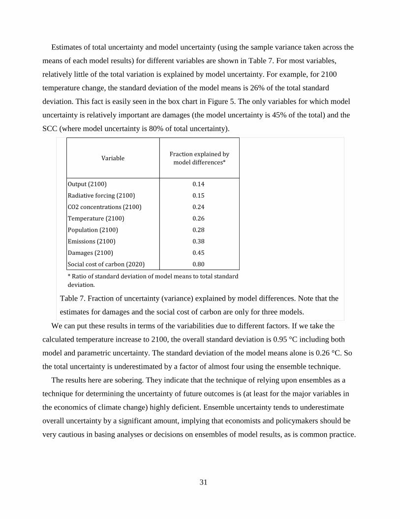
31
Estimates of total uncertainty and model uncertainty (using the sample variance taken across the
means of each model results) for different variables are shown in Table 7. For most variables,
relatively little of the total variation is explained by model uncertainty. For example, for 2100
temperature change, the standard deviation of the model means is 26% of the total standard
deviation. This fact is easily seen in the box chart in Figure 5. The only variables for which model
uncertainty is relatively important are damages (the model uncertainty is 45% of the total) and the
SCC (where model uncertainty is 80% of total uncertainty).
We can put these results in terms of the variabilities due to different factors. If we take the
calculated temperature increase to 2100, the overall standard deviation is 0.95 °C including both
model and parametric uncertainty. The standard deviation of the model means alone is 0.26 °C. So
the total uncertainty is underestimated by a factor of almost four using the ensemble technique.
The results here are sobering. They indicate that the technique of relying upon ensembles as a
technique for determining the uncertainty of future outcomes is (at least for the major variables in
the economics of climate change) highly deficient. Ensemble uncertainty tends to underestimate
overall uncertainty by a significant amount, implying that economists and policymakers should be
very cautious in basing analyses or decisions on ensembles of model results, as is common practice.
Table 7. Fraction of uncertainty (variance) explained by model differences. Note that the
estimates for damages and the social cost of carbon are only for three models.
VariableFraction explained by
model differences*
Output (2100) 0.14
Radiative forcing (2100) 0.15
CO2 concentrations (2100) 0.24
Temperature (2100) 0.26
Population (2100) 0.28
Emissions (2100) 0.38
Damages (2100) 0.45
Social cost of carbon (2020) 0.80
* Ratio of standard deviation of model means to total standard
deviation.

32
C. Reliability of the Estimates
One question that arises in developing a new approach is how well it performs. In addition to the
earlier Monte Carlo “out-of-sample” tests of the SRFs, we also tested the reliability of the estimates
using multiple samples and bootstrap techniques. We ran the basic Monte Carlo runs twenty times
with samples of 1 million to determine the stability of the results. The results are highly reliable in
the center of the distribution, with modest deterioration in the extreme tails. Two examples will
indicate the reliability. For the median of the Monte Carlo estimates of 2100 temperature, the
standard error of the median for the six models averages 0.03% of the mean of the medians. For the
99.9 percentile of 2100 temperature, the standard error of the median averages 0.18% of the mean
of the 99.9 percentile. The variable with the lowest reliability is damages, which is also relatively
poorly predicted by the Monte Carlo estimates. The standard error of the median for the three
models is 0.22% of the mean of the medians, while the standard error of the 99th percentile for the
three models is 0.48% of the mean of the 99th percentile.
D. Sensitivity of the Results to Parameter Variability
Another important question is the extent to which the results are sensitive to the individual
pdfs for the uncertain parameters. To test for sensitivity, we performed an experiment where we
increased the standard deviation of each of the pdfs by a factor of 1.5, both one at a time and
together (holding the means constant). We then calculated the elasticity (the percentage change in
standard deviation of the output variable per percentage change in standard deviation of the
uncertain variable). As an example, increasing the standard deviation of the equilibrium climate
sensitivity by 50% increased the standard deviation of 2100 temperature by 19%, for an elasticity of
0.39. This is less than unity because the temperature does not respond proportionally to ECS during
a time period of a century.
Table 8 shows the elasticities for all major variables and for different combinations of the
uncertain parameters, taking the average of the 6 models. Increasing all uncertainties together has
an elasticity of around one, sometimes higher and sometimes lower. The difference from one in the
bottom row arises because of non-linearities in the structural equations of the models.
Increasing population uncertainty has a small effect on all variables except population. Increasing
equilibrium temperature uncertainty has a moderate elasticity on temperature but has no significant
effect on other variables. The major sensitivity is TFP uncertainty. The elasticities here (except for
unaffected population) vary from 0.57 for temperature to 1.60 for damages. Note that this elasticity
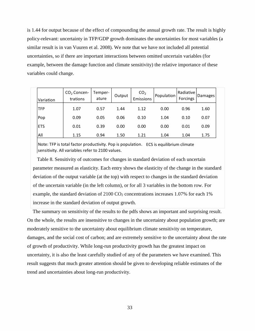
33
is 1.44 for output because of the effect of compounding the annual growth rate. The result is highly
policy-relevant: uncertainty in TFP/GDP growth dominates the uncertainties for most variables (a
similar result is in van Vuuren et al. 2008). We note that we have not included all potential
uncertainties, so if there are important interactions between omitted uncertain variables (for
example, between the damage function and climate sensitivity) the relative importance of these
variables could change.
The summary on sensitivity of the results to the pdfs shows an important and surprising result.
On the whole, the results are insensitive to changes in the uncertainty about population growth; are
moderately sensitive to the uncertainty about equilibrium climate sensitivity on temperature,
damages, and the social cost of carbon; and are extremely sensitive to the uncertainty about the rate
of growth of productivity. While long-run productivity growth has the greatest impact on
uncertainty, it is also the least carefully studied of any of the parameters we have examined. This
result suggests that much greater attention should be given to developing reliable estimates of the
trend and uncertainties about long-run productivity.
Table 8. Sensitivity of outcomes for changes in standard deviation of each uncertain
parameter measured as elasticity. Each entry shows the elasticity of the change in the standard
deviation of the output variable (at the top) with respect to changes in the standard deviation
of the uncertain variable (in the left column), or for all 3 variables in the bottom row. For
example, the standard deviation of 2100 CO2 concentrations increases 1.07% for each 1%
increase in the standard deviation of output growth.
Variation
CO2 Concen-
trations
Temper-
atureOutput
CO2
EmissionsPopulation
Radiative
ForcingsDamages
TFP 1.07 0.57 1.44 1.12 0.00 0.96 1.60
Pop 0.09 0.05 0.06 0.10 1.04 0.10 0.07
ETS 0.01 0.39 0.00 0.00 0.00 0.01 0.09
All 1.15 0.94 1.50 1.21 1.04 1.04 1.75
Note: TFP is total factor productivity. Pop is population. ETS is equilibrium temperature
sensitivity. All variables refer to 2100 values.
ECS is equilibrium climate

34
VIII. Conclusions
It is well understood in the economics of climate change that uncertainty is one of the greatest
challenges, bedeviling policymakers and stimulating a growing academic literature. This study is
the first analysis of multiple major integrated assessment models of climate change to explore
baseline uncertainty in key parameters. The approach is based on estimating classic statistical
forecast uncertainty.
The approach consists of two tracks. Track I involves performing a set of model calibration runs
for six models and three key uncertain parameters, and estimating surface response functions for the
results of those runs. Track II involves developing pdfs for the three uncertain parameters. The two
tracks are brought together through a set of Monte Carlo simulations to estimate the output
distributions of multiple output variables that are important for climate change and climate-change
policy. This approach is replicable and transparent, and overcomes several feasibility obstacles for
examining uncertainty in baseline trajectories for use in climate policy analysis.
Here are the key results. First, the central projections of the integrated assessment models (IAMs)
are remarkably similar at the modeler’s baseline parameters. This result is probably due to the fact
that models have been used in model comparisons and may have been revised to yield similar
baseline results. However, the projections diverge sharply when alternative assumptions about the
key uncertain parameters are used, especially at high levels of population growth, productivity
growth, and equilibrium climate sensitivity.
Second, despite these differences across models for alternative parameters, the distributions of
the key output variables are remarkably similar across models with very different structures and
levels of complexity. To take year 2100 temperature as an example, the quantiles of the
distributions of the models differ by less than ½ °C for the entire distribution up to the 95th
percentile. Third, we find that the climate-related variables are characterized by low uncertainty
relative to those relating to most economic variables. For this comparison, we look at the coefficient
of variation (CV) of the Monte Carlo simulations. As shown in Table 3, CO2 concentrations,
radiative forcings, and temperature (all for 2100) have relatively low CV. Output and damages have
relatively high CV. As examples, the model-average coefficient of variation for carbon dioxide
concentrations in 2100 is 0.28, while the coefficient of variation for climate-change damages is
1.30. The social cost of carbon has an intermediate CV within models, but when model variation is
included, the CV of the SCC is close to that of output and damages. These results highlight the

35
importance of research on economic relationships and damage functions underpinning the models
for reducing uncertainty and improving policymaking (see Pizer et al. 2014 and Drouet et al. 2015).
Fourth, we find much greater parametric (within-model) uncertainty than structural (across-
model) uncertainty for all output variables except the social cost of carbon. For example, in
examining the uncertainty in 2100 temperature increase, the difference of model means (across-
model or what is sometimes called the ensemble uncertainty) is approximately one-quarter of the
total uncertainty, with the rest associated with parametric uncertainty. While looking across six
models by no means spans the space of methods, the six models examined here are representative of
the differences in size, structure, and complexity of IAMs. This result is important because of the
widespread use of ensemble uncertainty as a proxy for overall uncertainty and highlights the need
for a re-orientation of research towards examining parametric uncertainty across multiple models.
Fifth, we find that within a wide range of uncertainty, changes in dispersion of two of the
uncertain parameters taken singly have a relatively small effect on the uncertainty of the output
variables, these being population growth and equilibrium climate sensitivity. However, uncertainty
about productivity growth has a major impact on the uncertainty of all the major output variables.
The reason for this is that the uncertainty of productivity growth compounds greatly over the 21st
century and induces an extremely large uncertainty about output, emissions, concentrations,
temperature change, and damages by the end of the century.
As in any study, this analysis is sharply focused. By analyzing parametric uncertainty in three
key parameters, we clearly cannot estimate all the uncertainties in climate change. As we describe
above, there are many uncertainties that cannot be captured using the statistical framework
developed here. For example, analysis focused on different modeling approaches to damages could
help provide insight into one of the key uncertainties not addressed in this study. But by providing
detailed estimates of uncertainty across a range of IAMs that are currently being used in the policy
process, we believe that we have significantly improved the understanding of uncertainty in the
economics of climate change. Moreover, our new two-track approach is well-suited for expansion to
additional parameters and models, and can be readily used to explore additional concerns, such as
the effect of interaction between carbon policies and uncertainty.

36
REFERENCES
Anderson, Barry, Emanuele Borgonovo, Marzio Galeotti, Roberto Rosen. 2014. “Uncertainty in
Climate Change Modeling: Can Global Sensitivity Analysis be of Help? Risk Analysis 34: 271-
293.
Annan, James D. and Julia C. Hargreaves. 2006. Using Multiple Observationally-based Constraints
to Estimate Climate Sensitivity. Geophysical Research Letters 33(6): L06704.
Anthoff, David, and Richard Tol. 2010. On International Equity Weights and National Decision
Making on Climate Change. Journal of Environmental Economics and Management 60(1): 14-20.
Anthoff, David, and Richard Tol. 2013. The Uncertainty about the Social Cost of Carbon: A
Decomposition Analysis Using FUND. Climatic Change 117(3): 515-530.
Armstrong, J. Scott. 2001. Combining forecasts. Principles of forecasting. Springer US, 417-439.
Baker, Erin. 2005. Uncertainty and Learning in a Strategic Environment: Global Climate Change.
Resource and Energy Economics 27(1): 19-40.
Batchelor, Roy, and Pami Dua. 1995. Forecaster diversity and the benefits of combining forecasts.
Management Science 41: 68-75.
Barro, Robert and José F. Ursua. 2010. Barro-Ursua Macroeconomic Data. rbarro.com/data-sets.
Blanford, Geoff, James Merrick, Richard Richels, and Steven Rose. 2014. Trade-offs Between
Mitigation Costs and Temperature Change. Climatic Change 123(3-4): 527-541.
Bosetti, Valentina, Carlo Carraro, Marzio Galeotti, Emanuele Massetti, and Massimo Tavoni. 2006.
WITCH: A World Induced Technical Change Hybrid Model. Energy Journal 27(SI2): 13-37.
Bosetti, Valentina, Carlo Carraro, Emanuele Massetti, and Massimo Tavoni. 2014. Climate Change
Mitigation, Technological Innovation and Adaptation: Edward Elgar Publishers.
Calvin, Katherine, et al. 2011. GCAM Documentation, http://www.globalchange.umd.edu/gcam/.
College Park, MD: Joint Global Change Research Institute.
CBO. 2005. Uncertainty in Analyzing Climate Change: Policy Implications. Washington, DC:
Congressional Budget Office.
Chen, Y.-H., Sergey Paltsev, John M. Reilly, Jennifer F. Morris, and Mustafa H. Babiker. 2016.
Long-Term Economic Modelling for Climate Change Assessment. Economic Modelling. 52(B):
867-883.
Christensen, Peter, Kenneth Gillingham, William Nordhaus. 2018. Uncertainty in Long-run
Forecasts of Productivity Growth. Yale University Working Paper.
37
Clemen, Robert T., and Robert L. Winkler. 1999. Combining probability distributions from experts
in risk analysis. Risk Analysis 19(2): 187-203.
Clements, Michael, and David Hendry. 1998. Forecasting Economic Time Series. Cambridge, UK:
Cambridge University Press.
Clements, Michael, and David Hendry. 1999. Forecasting Non-stationary Economic Time Series.
Cambridge, MA: MIT Press.
Drouet, Laurent, Valentina Bosetti, and Massimo Tavoni. 2015. Selection of Climate Policies Under
the Uncertainties in the Fifth Assessment Report of the IPCC. Nature Climate Change 5: 937-940.
Edmonds, Jae, and John Reilly. 1983a. Global Energy and CO2 to the Year 2050. Energy Journal
4(3): 21-47.
Edmonds, Jae, and John Reilly. 1983b. Global Energy Production and Use to the Year 2050. Energy
8(6): 419-432.
Edmonds, Jae, and John Reilly. 1983c. A Long-term Global Energy-economic Model of Carbon
Dioxide Release From Fossil Fuel Use. Energy Economics 5(2): 74-88.
Ericsson, Neil. 2001. Forecast Uncertainty in Economic Modeling. Washington, DC: Board of
Governors of the Federal Reserve System International Finance Discussion Papers.
Greenstone, Michael, Elizabeth Kopits, and Ann Wolverton. 2013. Developing a Social Cost of
Carbon for US Regulatory Analysis: A Methodology and Interpretation. Review of Environmental
Economics and Policy 7(1): 23-46.
Hammersley, John M., and David C. Handscomb. 1964. Monte Carlo Methods. New York: John
Wiley and Sons.
Hegerl, Gabriele, Thomas C. Crowley, William T. Hyde, and David J. Frame. 2006. Climate
Sensitivity Constrained by Temperature Reconstructions Over the Past Seven Centuries. Nature
440: 1029-1032.
IWG. 2013. Technical Support Document: Technical Update of the Social Cost of Carbon for
Regulatory Impact Analysis Under Executive Order 12866. Washington, DC: Interagency
Working Group on the Social Cost of Carbon.
InterAcademy Council. 2010. Climate Change Assessments: Review of the Processes and
Procedures of the IPCC, 2010, Harold Shapiro, chair.
IPCC. 2014. Fifth Assessment Report of the Intergovernmental Panel on Climate Change.
Cambridge, UK and New York, NY: Cambridge University Press.

38
Jensen, Svenn and Christian Traeger. 2014. Optimal Climate Change Mitigation under Long-Term
Growth Uncertainty: Stochastic Integrated Assessment and Analytic Findings. European
Economic Review 69(C): 104-125.
Kelly, David and Zhuo Tan. 2015. Learning and Climate Feedbacks: Optimal Climate Insurance
and Fat Tails. Journal of Environmental Economics & Management 72: 98-122.
Knutti, Reto, and Gabriele Hegerl. 2008. The Equilibrium Sensitivity of the Earth's Temperature to
Radiation Changes. Nature Geoscience 1: 735-743.
Lemoine, Derek, and Haewon McJeon. 2013. Trapped Between Two Tails: Trading Off Scientific
Uncertainties via Climate Targets. Environmental Research Letters 8: 1-10.
Lemoine, Derek and Ivan Rudik. 2017. Managing Climate Change Under Uncertainty: Recursive
Integrated Assessment at an Inflection Point. Annual Review of Resource Economics.
forthcoming.
Lemoine, Derek and Christian Traeger. 2014. Watch Your Step: Optimal Policy in a Tipping
Climate. American Economic Journal: Economic Policy. 6(1): 137-166.
Lenton, Timothy, Hermann Held, Elmar Kriegler, Jim Hall, Wolfgang Lucht, Stefan Rahmstorf, and
Hans Joachim Schellnhuber. 2008. Tipping Elements in the Earth's Climate System. Proceedings
of the National Academy of Sciences. 105(6): 1786-1793.
Libardoni, Alex and Christopher Forest. 2013. Correction to ‘Sensitivity of Surface Distributions of
Climate System Properties to the Surface Temperature Data Set’. Geophysical Research Letters
40(10): 2309-2311.
Lutz, Wolfgang, William Butz, and Samir KC. 2014. World Population and Human Capital in the
Twenty-First Century. Oxford, UK: Oxford University Press.
Lutz Wolfgang, Warren Sanderson, Sergei Scherbov. 2001. The End of World Population Growth.
Nature 412, 543-545.
Lutz, Wolfgang, Warren Sanderson, and Sergei Scherbov. 2008. IIASA's 2007 Probabilistic World
Population Projections, IIASA World Population Program Online Data Base of Results.
Available from
http://www.iiasa.ac.at/web/home/research/researchPrograms/WorldPopulation/Reaging/2007_upd
ate_prob_world_pop_proj.html.
Maddison, Angus. 2003. The World Economy: Historical Statistics. OECD, Paris, France.
Manne, Alan, Robert Mendelsohn, and Richard Richels. 1999. MERGE: A Model for Evaluating
Regional and Global Effects of Greenhouse Gas Reduction Policies. Energy Policy 23(1): 17-34.

39
Meinshausen, Malte, Thomas Wigley, and Sarah C. Raper. 2011. Emulating Coupled Atmosphere-
Ocean and Carbon Cycle Models with a Simpler Model, MAGICC6 - Part I: Model Description
and Calibration. Atmospheric Chemistry and Physics 11: 1417-1456.
Muller, Ulrich and Mark W. Watson. 2016. Measuring Uncertainty about Long-Run Predictions.
Review of Economic Studies, 83(4): 1711-1740.
Nordhaus, William. 2008. A Question of Balance: Weighing the Options on Global Warming
Policies. New Haven, CT: Yale University Press.
Nordhaus William. 2014. Estimates of the Social Cost of Carbon: Concepts and Results from the
DICE-2013R Model and Alternative Approaches. Journal of the Association of Environmental
and Resource Economists, 1, 273-312.
Nordhaus, William, and David Popp. 1997. What is the Value of Scientific Knowledge? An
Application to Global Warming Using the PRICE Model. Energy Journal 18(1): 1-45.
Nordhaus, William, and Paul Sztorc. 2014. DICE 2013: Introduction and User's Manual. New
Haven, CT: Yale University.
NRC. 2000. Beyond Six Billion: Forecasting the World's Population. Washington, DC: National
Academy Press.
O'Neill, Brian, Deborah Balk, Melanie Brickman, and Markos Ezra. 2001. A Guide to Global
Population Projections. Demographic Research 4(8): 203-288.
Olsen, Roman, Ryan Sriver, Marlos Goes, Nathan Urban, H. Damon Matthews, Murali Haran, and
Klaus Keller. 2012. A Climate Sensitivity Estimate Using Bayesian Fusion of Instrumental
Observations and an Earth System Model. Geophysical Research Letters 117(D04103): 1-11.
Peck, Stephen, and Thomas Teisberg. 1993. Global Warming Uncertainties and the Value of
Information: An Analysis Using CETA. Resource and Energy Economics 15(1): 71-97.
Pizer, William 1999. Optimal Choice of Climate Change Policy in the Presence of Uncertainty.
Resource and Energy Economics. 21(3-4): 255-287.
Pizer, William, Matthew Adler, Joseph Aldy, David Anthoff, Maureen Cropper, Kenneth
Gillingham, Michael Greenstone, Brian Murray, Richard Newell, Richard Richels, Arden Rowell,
Stephanie Waldhoff, and Jonathan Wiener. 2014. Using and Improving the Social Cost of Carbon.
Science 346(6214): 1189-1190.
Ramsey, Frank. 1931. Truth and Probability. In The Foundations of Mathematics and Other Logical
Essays, edited by Richard Bevan Braithwaite, 156-198. London, UK: Kegan, Paul, Trench,
Trubner and Company.

40
Reilly, John, Jae Edmonds, R. Gardner, A. Brenkert. 1987. Monte Carlo Analysis of the
IEA/ORAU Energy/Carbon Emissions Model. Energy Journal 8:1-29.
Robinson, Alexander, Reinhard Calov, and Andrey Ganopolski. 2012. Multistability and Critical
Thresholds of the Greenland Ice Sheet. Nature Climate Change 2: 429-432.
Rytgaard, Mette. 1990. Estimation in the Pareto distribution. Astin Bulletin 20.02: 201-216.
Savage, Leonard. 1954. The Foundations of Statistics. New York: John Wiley and Sons.
Sokolov, A., Peter H. Stone, Christopher Forest, Ronald Prinn, Marcus Sarofim, Mort Webster,
Sergei Paltsev, Adam Schlosser, David Kicklighter, Stephanie Dutkiewicz, John Reilly, Chien
Wang, Benjamin Felzer, Jerry Melillo, and Henry Jacoby. 2009. Probabilistic Forecast for 21st
Century Climate Based on Uncertainties in Emissions (without Policy) and Climate Parameters.
Journal of Climate 22(19): 5175-5204.
Tol, Richard. 1997. On the Optimal Control of Carbon Dioxide Emissions - An Application of
FUND. Environmental Modelling and Assessment, 2: 151-163.
Webster, Mort. 2002. The Curious Role of Learning: Should We Wait for More Data? Energy
Journal 23(2): 97-119.
Webster, Mort, Mustafa Babiker, M. Mayer, John Reilly, Jochen Harnisch, Marcus Sarofim, and
Chien Wang. 2002. Uncertainty in Emissions Projections for Climate Models. Atmospheric
Environment 36(22): 3659-3670.
Webster, Mort, Andrei Sokolov, John Reilly, Christopher Forest, Sergei Paltsev, Adam Schlosser,
Chien Wang, David Kicklighter, Marcus Sarofim, Jerry Melillo, Ronald Prinn, and Henry Jacoby.
2012. Analysis of Climate Policy Targets Under Uncertainty. Climatic Change 112(3-4): 569-583.