Calhoun: The NPS Institutional Archive

Theses and Dissertations Thesis Collection

1988

Modelling DD-963 Class material readiness

Will, Jonathan E.

http://hdl.handle.net/10945/23075

^UATE SCHOOL'^^~rA 93943-6002

NAVAL POSTGRADUATE SCHOOL

Monterey , California

THESIS

MODELLING DD-963 CLASS MATERIAL |

READINESS

by

•

Jonathan E . Will

September 1988

Thesis Advisor: Dan C. Boger

Distribution limited to U.S. Government Agencies and their Contractors;Administrative Operational Use; September 1988. Other requests for this documentshall be referred to Superintendent, Code 043, Naval Postgraduate School, Monterey,CA 93943-5000 via the Defense Technical Information Center, Cameron Station,Alexandria, VA 22304-6145.

DESTRUCTION' NOTICE - Destroy by any method that will prevent disclosure ofcontents or reconstruction of the document.

T242434

nclassified

:unt> classification of this page

REPORT DOCIMENTATION PAGE1 Report Security Classification Lnclassified lb Restrictive Markings

i SecuritN Classification Authoniv

3 Declassification Downgrading Schedule

3 Distribution Availability of Report Distribution LuTUted tO U.S.

Government Agencies and their Contractors:

Administrative Operational Use; September 1988. Other

requests for this document shall be referred to

Superintendent, Code 043, Naval Postgraduate School,

Monterey, CA 93943-5000 via the Defense Technical

Information Center, Cameron Station, Alexandria, VA22304-6145.

Perforrrung Organization Report .Number(s) 5 Monitoring Organization Report Number(s)

a Name of Performing Organization

>aval Postgraduate School

6b Office Symbol

(if applicable) 30

7a Name of Monitoring Organization

Naval Postgraduate School

: Address (dry. siaie, and ZIP code)

lonterey, CA 93943-50007b Address (dry. siaie. and ZIP code)

Monterev, CA 93943-5000

\ Name of Funding Sponsoring Organization 8b Office Symbol( if applicable

)

9 Procurement Instrument Identification Number

Address (d:y. s:aie, and ZIP codej 10 Source of Funding Numbers

Program Element No Project No Task No Work Unit .Accession No

I Title (include security ciassificafion I MODELLING DD-963 CLASS MATERIAL READINESS

I Personal Authorfs) Jonathan E. Will

!a Type of Report

laster's Thesis

13b Time CoveredFrom To

14 Date of Report (year, monih, dav)

September 1988

15 Page Count52

) Supplementary Notation The views expressed in this thesis are those of the author and do not reflect the official policy or

osition of the Department of Defense or the U.S. Government^

Cosati Codes

leld Group Subgroup

IS Subject Terms i continue on re\erse if necessary and identify by block number)

thesis, regression, readiness, model.

} Abstract (continue on reverse if necessary and identify by block number)

This thesis develops several simple statistical models of DD-963 Class material readiness using data from 1981 to 1986.

he models are exercised to demonstrate their ability to explain and predict surface warship material readiness. Ability to

)recast future readiness is found to be low. Two different measures of readiness are compared and found to be redundant,

.ccurately measured data on personnel mamiing. resources spent on ship repair and resources spent on sliip modernization

3uld be useful in improving the sliip material readiness models developed here.

) Disinbuiion Availability of Abstract

] unclassified unlimited D same as report D DTIC users

21 Abstract Security Classification

Unclassified

'a Name of Responsible Individual

'an C. Boser22b Telephone (include Area code}

(408) 646-2706

22c Office Svmbol

54Bo

D FORM 1473.84 mar 83 APR edition may be used until exhausted

All other editions are obsolete

security classification of this page

Unclassified

Distribution limited to U.S. Government Agencies and their Contractors;

Administrative Operational Use; September 198S. Other requests for this document

shall be referred to Superintendent, Code 043, Naval Postgraduate School, Monterey,

CA 93943-5000 via the Defense Technical Information Center, Cameron Station,

Alexandria, VA 22304-6145.

Modelling DD-963 Class Material Readiness

by

Jonathan E^^Will

Lieutenant Commander, United States Na\7B.S., U. S. Naval Academy, 1978

Submitted in partial fulfillment of the

requirements for the degree of

MASTER OF SCIENCE IN OPER-\TIONS RESEARCH

from the

NAVAL POSTGR,\DUATE SCHOOLSeptember 19SS

ABSTRACT

This thesis develops several simple statistical models of DD-963 Class material

readiness using data from 1981 to 1986. The models are exercised to demonstrate their

ability to explain and predict surface warship material readiness. Ability to forecast fu-

ture readiness is found to be low. Two different measures of readiness are compared and

found to be redundant. Accurately measured data on personnel manning, resources

spent on ship repair and resources spent on ship modernization could be useful in im-

proving the ship material readiness models developed here.

m

TABLE OF CONTENTS

I. INTRODUCTION 1

A. BACKGROUND 1

B. PURPOSE 2

II. DATA 3

A. VAMOSC DATA 3

B. CNA DATA 4

C. COMMENTS ABOUT THE DATA 5

III. MODELS 7

A. PRIMARY MODEL 7

1. Relationships of Explanaton^ Variables to Readiness 8

2. Redundancy of Some Explanaton* Variables 9

3. Determination of Probable Signs of CoefTicients in Model 9

B. ALTERNATE MODEL 10

IV. ANALYSIS OF PRIMARY MODEL 11

A. EXPLORATORY DATA ANALYSIS 11

B. ORDINARY LEAST SQUARES REGRESSION 12

C. DEVELOPING THE PRIMARY MODEL-ITERATIVE APPROACH . . 14

1. Delayed EfTects of Explanatory Variables 15

2. Consideration of Other Explanatory Variables 16

3. Consideration of Data Transformations 17

4. VAMOSC Data 17

5. Initial Model Resuhs 18

6. VAMOSC Data Problems 19

a. Multicollinearity 19

b. Checking for Stability 21

D. INTER.MEDIATE PRIMARY MODEL 23

E. FINAL PRIMARY MODEL 25

F. EXAMINATION OF ASSUMPTIONS 27

IV

DUj

1. Checking for Structural Change 28

2. Transformed Model 29

V. ANALYSIS OF ALTERNATE MODEL 31

A. ALTERNATE PREDICTION MODEL 33

VI. CONCLUSIONS 36

A. COMPARISON OF MEASURES OF READINESS 36

B. USEFUL EXPLANATORY VARIABLES 36

C. DATA COLLECTION 37

D. GENERAL CONCLUSIONS 37

APPENDIX DESCRIPTION OF VARIABLES 38

LIST OF REFERENCES 42

INITIAL DISTRIBUTION LIST 43

LIST OF TABLES

Table 1. INITIAL PRIMARY MODEL RESULTS 19

Table 2. LINEAR CORRELATION COEFFICIENTS 20

Table 3. MULTICOLLINEARITY EFFECTS ON REGRESSION RESULTS . 21

Table 4. INTERMEDIATE PRIMARY MODEL RESULTS 23

Table 5. PRIMARY PREDICTION MODEL RESULTS 26

Table 6. INTERMEDIATE ALTERNATE MODEL RESULTS 33

Table 7. ALTERNATE PREDICTION MODEL RESULTS 34

VI

LIST OF FIGURES

Figure 1. Sample Data Plot 12

Figure 2. Sample Data Plot 13

Figure 3. Personnel Data Problems 17

Figure 4. Illustration of High Leverage Points 22

Figure 5. Demonstration orPrimar>' Model 24

Figure 6. Demonstration of Primar\' Prediction Model 27

Figure 7. Results of Retransformation 30

Figure 8. Relation between Primar\- and Alternate Readiness Measures 32

Figure 9. Results of Alternate Prediction Model 35

vu

I. INTRODUCTION

A. BACKGROUND

The \a\7 maintains a large force of ships, submarines and aircraft to perform its

assignments. At any one time, however, not all of these are able to operate as designed;

some have material casualties (i.e., broken equipment) that reduce their effectiveness,

and others are in planned maintenance periods for upgrading and repair. The units which

can operate as designed are termed "ready."

Overall readiness can be defined as the ability of a Navy unit to perform all its de-

signed missions. Material readiness--the ability of all the unit's equipment to function

as designed--is a component of overall readiness.

Since a small combat force with high material readiness is the short-term equivalent

of a much larger force with low readiness, it is desirable to maintain high levels of ma-

terial readiness. Doing this requires money-to buy spare parts, to pay for the mainte-

nance facilities that the Nasy operates, etc. Therefore, the Navy's budget limits the

readiness that can be achieved. Within existing budget constraints, the Navy wants to

maximize the readiness of its forces.

For several years, the Program Resource Appraisal Division of the Office of the

Chief of Naval Operations (OP-81) has used a mathematical model to predict the mate-

rial readiness of Navy aircraft. As inputs, the model takes planned funding in various

categories of aircraft maintenance and repair. The output of the model is the predicted

proportion of the Navy's aircraft which will be able to perform all designed missions-

the "Fully Mission Capable" (FMC) rate. The FMC concept is widely used and accepted

in the Naval aviation community. The model has been helpful in determining budget

needs and in allocating funds to meet FMC goals. It gives insight into which areas of

the budget result in the biggest improvements in aircraft FMC rate per dollar spent.

A similar model designed for use with surface ships is needed. The same model

cannot be used because a ship is a fundamentally different combat system from an air-

craft. The Surface Warfare community has no concept analogous to the aviation FMCrate, so a measure of surface ship material readiness (hereafter referred to simply as

readiness) is needed. OP-81 has created such a measure by using the Navy's existing

Casualty Report (CAS REP) system.

A CASREP is a message sent from a ship's Commanding Officer to his operational

and administrative chain of command when the ship experiences a material casualty that

the crew cannot fix within 48 hours. CASREPs are grouped into one of three categories

depending on the impact of the casualty. The C3 and C4 categories indicate a major

material casualty—an equipment failure that prevents the ship from performing one or

more of its primary missions (e.g., anti-submarine warfare, anti-air warfare, anti-surface

warfare, mobility, etc.). CASREPs are considered a reliable indicator of the ship's ma-

terial condition because of the visibility and importance of these official messages. By

definition, a ship without C3 or C4 CASREPs has no equipment problems that prevent

it from performing all of its primary' missions.

Over the past four years, OP-81 has engaged several defense contractors to develop

mathematical models of the relationship between resources (budget dollars) and ship

readiness using the time free of C3 and C4 CASREPs as the measure of ship readiness

[Refs. 1,2]. These models have varied in complexity and utility. Even after this work,

however, several questions of interest remain:

• Is there a "better" measure of surface ship material readiness?

• What variables can best explain and predict future surface ship material readiness?

• What data should be collected to support the use of such a model?

B. PURPOSE

The objective of this thesis is to develop two mathematical models of surface ship

material readiness. The first model will use the OP-81 measure of ship material read-

iness, the time free of C3 C4 CASREPs. The second model will use a related but different

measure of readiness, C3 and C4 CASREP-days. This measure simply sums over a fiscal

year the product of C3 and C4 CASREPS and the number of days on which each casu-

alty existed. For example, two C3 or C4 CASREPs lasting the entire year of 365 days

would result m 730 C3, C4 CASREP-days for that year.

The models will then be compared to see which one is better able to predict and

explain ship readiness. The process of developing these two models will help to answer

the questions listed above and give insight into the general problem of predicting ship

material readiness.

II. DATA

Data are needed on time free of C3/C4 CASREPs, on C3/C4 CASREP-days and on

potential explanatory' factors. Two data sets of interest are found. The first is obtained

from the Naval Sea Systems Command (NAVSEA). Entitled "Visibility and Manage-

ment of Operating and Support Costs, Ships" (VAMOSC), it was used by at least one

of the OP-81 contractors in building a complex ship readiness model [Ref 2:

pp.2T7-2'20]. The second data set is from the Center for Naval Analyses (CNA), enti-

tled "Factors Affecting Ship Material Condition." It is being used for ongoing studies

of ship equipment condition at CNA [Refs. 3, 4 , 5].

The VAMOSC data are unclassified, but parts of the CNA database are classified

at the Secret level. In order to keep this thesis at an unclassified/ Official Use Only level,

only unclassified data from the CNA database are used.

Both of these data sets are ver\' large, containing information on the entire fieet of

surface ships and submarines. To limit the breadth of the study, only one class of surface

ships is analyzed. The DD-963 (SPRL'ANCE) class of destroyers is chosen for several

reasons. The 31 ships in this class constitute a good sample size, and all but one of them

were in commission by 1980. The last ship was not commissioned until 1983 and is

therefore omitted from the study because of the resulting missing data.

A change in the reporting requirements for CASREPS took place in 1980. There-

fore, data from fiscal years 1981 to as recently as possible (1986) are used. Having 30

ships for each of the six years results in 180 data points for the study.

Each variable available for the study is hsted in the Appendix. A general discussion

of the database and its structure follows.

A. VAMOSC DATAThe Visibility and Management of Operating and Support Costs, Ships (VAMOSC)

data set is maintained by NAVSEA to study and manage the costs of operating and

maintaining the ships in the Navy. It contains information on a fiscal-year basis on each

ship in the NavT. This information is held in both then-year dollars and constant dollars.

The form of constant Fiscal Year 1986 (FY-86) dollars is chosen for this study in order

to eliminate the effects of inflation.

About 100 separate variables are available for each hull. These data are in three

general categories:

• direct unit costs

• intermediate maintenance costs

• depot-level maintenance costs

Direct unit costs are the costs of operating the ship (paying the crew, buying fuel,

etc.) and the costs of organization-level maintenance (repairs performed by the ship's

crew) and are broken down into three classifications-personnel, material and purchased

services. Material includes fuel, lubricants, repair parts and supplies. About 30 variables

are available on each ship in this categon.'.

Intermediate maintenance costs are costs involved in ship repair performed by the

Navy's intermediate-level maintenance facilities, which include all tenders and repair

ships as well as the Shore Intermediate Maintenance Activities. Money spent on each

ship is broken down according to whether the maintenance activity is afloat or ashore,

and is further divided into the areas of labor and material. Six variables are available in

this category.

Depot-level maintenance is repair work performed by organizations with facilities

and skills equivalent to the original shipbuilder. These organizations include shipyards

(both publicly and privately owned) and the overseas Ship Repair Facilities operated by

the Na\y in the Pacific Ocean. This categor}' has the majority of the information held

by the VAMOSC database-about 65 variables are available for each ship. This infor-

mation is broken down into four groups: scheduled repairs (regular overhauls and se-

lected restricted availabilities), unscheduled repairs (restricted and technical

availabilities), fleet modernization program, and other (including Naval Aviation Depot

work).

Each of these groups is broken down into money spent in public shipyards, private

shipyards or ship repair facihties. For the publicly owned facilities, the money spent is

further broken down into labor, material and overhead. This information is not available

for private shipyards for proprietar\' reasons.

B. CNA DATA

Some of the data from CNA is similar in nature to the VAMOSC data, but the

structure of the CNA database is difTerent-lhe basic unit of CNA data is a month in-

stead of a fiscal year. The CNA data are generally of a more detailed nature than the

VAMOSC data, which are ver\' general.

In order to use these two data sets together, it is necessar\' to process the CNA data

to give it a fiscal year structure.

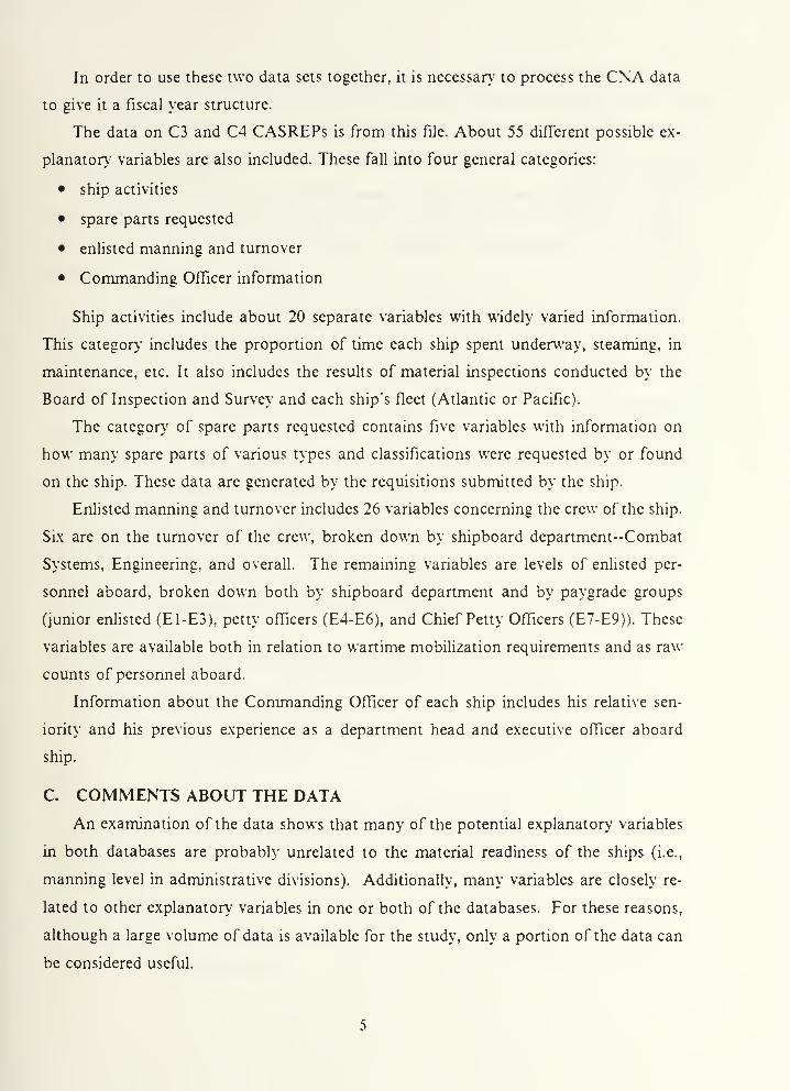
The data on C3 and C4 CASREPs is from this file. About 55 different possible ex-

planatory variables are also included. These fall into four general categories:

• ship activities

• spare parts requested

• enlisted manning and turnover

• Commanding Officer information

Ship activities include about 20 separate variables with widely varied information.

This category includes the proportion of time each ship spent unden^'ay, steaming, in

maintenance, etc. It also includes the results of material inspections conducted by the

Board of Inspection and Survey and each ship's fleet (Atlantic or Pacific).

The categor}^ of spare parts requested contains five variables with information on

how many spare parts of various types and classifications were requested by or found

on the ship. These data are generated by the requisitions submitted by the ship.

Enlisted manning and turnover includes 26 variables concerning the crew of the ship.

Six are on the turnover of the crew, broken down by shipboard department-Combat

Systems, Engineering, and overall. The remaining variables are levels of enlisted per-

sonnel aboard, broken down both by shipboard department and by paygrade groups

(junior enlisted (E1-E3), petty officers (E4-E6), and Chief Petty Officers (E7-E9)). These

variables are available both in relation to wartime mobilization requirements and as raw

counts of personnel aboard.

Information about the Commanding Officer of each ship includes his relative sen-

iority and his previous experience as a department head and executive officer aboard

ship.

C. COMMENTS ABOUT THE DATA

An examination of the data shows that many of the potential explanatory variables

in both databases are probably unrelated to the material readiness of the ships (i.e.,

manning level in administrative divisions). Additionally, many variables are closely re-

lated to other explanatory variables in one or both of the databases. For these reasons,

although a large volume of data is available for the study, only a portion of the data can

be considered useful.

The VAMOSC database has been approved by the Chief of Naval Operations for

fiscal decision-making purposes. This fact gives some confidence that the data it contains

are reliable. The CNA data have not been approved for decision-making purposes but

are also expected to be of relatively high quality because of their previous use and re-

fmement at CNA.

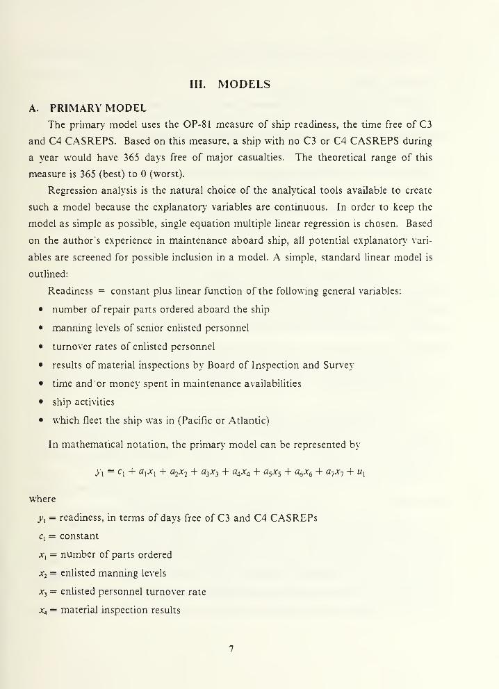
III. MODELS

A. PRIMARY MODELThe primary model uses the OP-81 measure of ship readiness, the time free of C3

and C4 CASREPS. Based on this measure, a ship with no C3 or C4 CASREPS during

a year would have 365 days free of major casualties. The theoretical range of this

measure is 365 (best) to (worst).

Regression analysis is the natural choice of the analytical tools available to create

such a model because the explanator\" variables are continuous. In order to keep the

model as simple as possible, single equation multiple linear regression is chosen. Based

on the author's experience in maintenance aboard ship, all potential explanator>^ vari-

ables are screened for possible inclusion in a model. A simple, standard linear model is

outlined:

Readiness = constant plus linear function of the following general variables:

• number of repair parts ordered aboard the ship

• manning levels of senior enlisted personnel

• turnover rates of enlisted personnel

• results of material inspections by Board of Inspection and Survey

• time and or money spent in maintenance availabilities

• ship activities

• which fleet the ship was in (Pacific or Atlantic)

In mathematical notation, the primar}' model can be represented by

where

y^ = readiness, in terms of days free of C3 and C4 CASREPs

c, = constant

jc, = number of parts ordered

Xi = enlisted manning levels

Xi = enlisted personnel turnover rate

x^ = material inspection results

A-j = resources expended in maintenance

X(, = ship activities

X. = fleet of ship

Wi = disturbance term: eflects of random fluctuations and excluded explanator\' vari-

ables

and where the a, represent the coefficients of the corresponding x, in this linear model.

A constant is necessarv' in this model to account for a baseline level of days free of

C3 and C4 CASREPs, with the explanatory' variables present to adjust this baseline.

1. Relationships of Explanator} Variables to Readiness

The general categories of explanatory' variables are chosen because each is re-

lated in some way to material readiness. For example, number of repair parts ordered is

clearly linked with corrective maintenance--more repair parts ordered implies that more

equipment is breaking.

High manning levels of senior enlisted personnel (E4-E6 and E7-E9) -the ex-

perienced repairmen aboard ships--provide required numbers and quality of people for

timely correction of material problems. Higher turnover rates of these personnel result

in more time required to fix casualties because some casualties recur, and the "corporate

memory" of men who have been part of the crew for a year or more is extremely helpful.

In-depth material inspections provide a good measure of the quality of the pre-

ventive maintenance program aboard a ship, and reflect the current material conditions

aboard the ship.

Ship activities can have a considerable effect on the ship's material condition.

The age of the ship, the length of time since its last overhaul and its operational status

(forward-deployed ships get priority treatment when they experience material casualties)

are examples of these factors.

Atlantic and Pacific fleets operate in somewhat different physical and leadership

environments, causing a possible geographical bias in CASREPs filed.

The relationships between maintenance and readiness are the most complex.

During most maintenance periods, two basic activities are performed-repair of broken

equipment and installation of new or upgraded ship systems. These two activities have

different effects on the material readiness of the ship. Repairs tend to terminate

CASREPs, and alterations tend to generate CASREPs when the new (and usually more

complex) ship systems fail at some time in the future. Repair and alteration activities

take place simultaneously, so it may be difficult to discriminate between CASREP gen-

eration and CASREP termination effects.

There is also a difference in the extent of modifications done by shipyards and

tenders. Major modifications to ship systems are generally performed by shipyards. Be-

cause of their inherent complexity, these modifications will often lead to material failures

later in the ship's life. Modifications accomplished by tenders tend to be relatively minor

in scope. The narrower extent of these modifications results in fewer later failures.

Distinguishing between the effects of major and minor modifications should be possible

since these are generally performed by different organizations.

Overall, more CASREPs require more maintenance.

2. Redundancy of Some Explanator}' Variables

For each of the seven general categories of potential explanator\' variables,

usually several related variables are actually available. For example, there are five dif-

ferent variables for number of repair parts ordered-depending on whether or not the

parts were in the ships Coordinated Shipboard Allowance List (COSAL). whether they

were in stock when requested, etc. About 80 variables are directly related to time and or

money spent in various types of maintenance. Only inspection results and fieet of ship

do not have multiple related variables.

Within each general categor}', one or more variables are chosen for inclusion in

the model. Each variable is chosen because it has a unique relationship with material

readiness. For example, in the family of repair parts ordered, the number o[ ordered

allowance list parts and ordered non-allowance hst parts normally stocked aboard the

ship is chosen because it is the best measure of significant equipment breakdown. No

other variable is picked from this family because these variables are ver>' closely related

and contain a high proportion of duplicate information. Each variable chosen from the

database in this way for inclusion in the model is marked with an asterisk in the Ap-

pendix.

3. Determination of Probable Signs of Coefficients in Model

The coefficients in a linear regression model can be regarded as partial deriva-

tives of the corresponding explanatory^ variables. That is, the coefficients represent the

amount of change in the response variable that would result from a unit change in the

corresponding explanator\' variable if all other explanatory variables are held constant.

Based on this interpretation of the coefficients and on the relationships between

the various explanatory' variables and readiness discussed above, the probable signs of

the coefficients {a, ) are determined. For example, number of repair parts ordered, turn-

over rates, time in maintenance, age of ship and time since overhaul should have a neg-

ative sign because all of these factors are related to more C3 and C4 CASREPs and thus

fewer days free of major CASREPs. Enlisted manning levels and inspection results

should have a positive coefficient because higher levels of these factors are related to

more days free of major casualties. The sign of the variable for fleet is uncertain since it

is not known which coast might be more likely to file CASREPs.

B. ALTERNATE MODELThe alternate model also uses C3 and C4 CASREPs as a measure of ship readiness,

but in a different way. Readiness is measured in terms of C3 and C4 CASREP-days per

year. For example, two C3 or C4 CASREPs lasting the entire year of 365 days would

result in 730 C3 C4 CASREP-days this year. The theoretical range of this measure starts

at zero (best possible) and is unbounded. It is important to investigate this alternate

measure of readiness because it could be more sensitive to multiple casualties than the

primary measure and might be easier to predict.

A mathematical representation of the alternate model is

Vj = C2 + b^.x^ + bjXi + 63A-3 + b^x^ + b^x^ + b^x^^ + b^x^ + Uj

where

Vj = readiness, in terms of C3 and C4 CASREP-days

Cj = constant (different from c, in primarv' model)

X, = explanatory' variables, as in primarv" model

b, = coefTicients of explanator\' variables

u. = disturbance term: effects of random fluctuations and excluded explanator>- vari-

ables

This model uses the same seven basic variables in a simple linear relationship. In

this case, however, the signs of the coefficients should be the opposite of the signs in the

primar\- model because the alternate model used an inverted measure of readiness. As

in the primar}' model, a constant is necessar}' to account for a baseline level of C3;C4

CASREP-davs.

10

IV. ANALYSIS OF PRIMARY MODEL

The first task, is to obtain the data sets from CNA and NAVSEA and to place them

in a usable form in the Naval Postgraduate School mainframe computer. An appropriate

software tool-FORTRAN, APL (A Programming Language) or the GRAFSTAT

graphics and statistics analysis package-is used at each stage of the analysis. Due to

different formats, times of receipt, and degree of difficulty in getting the data into the

mainframe computer, the CNA data are available for use considerably in advance of the

NAVSEA data. The CNA data are aggregated into a yearly structure to be compatible

with the NAVSEA data.

A. EXPLORATORY DATA ANALYSIS

The CNA data are first checked numerically and graphically to look for unusual or

nonsensical values. The bounded nature of many variables involved (for example, days

free of CASREPS, percent time in overhaul, enlisted manning levels, etc.) eases this task.

There are no cases of obvious incorrect values.

Simple plots are made of the various explanator}' variables against the time free of

C3 and C4 CASREPS. These plots show that some explanatory' variables have clear re-

lations to the dependent variable, but that most variables are not obviously related. Ex-

amples of these plots follow.

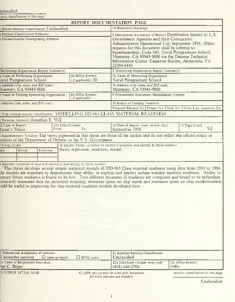
Figure 1 on page 12 shows an example of an explanatory" variable (repair parts or-

dered) that appears to have a relationship with the response variable, days free of C3 and

C4 CASREPS. It can be seen that the relationship is an inverted one-higher values of

repair parts ordered are correlated with lower values of days free of CASREPS. This

figure confirms the intuitive idea that the coefficient for repair parts ordered in the pri-

mary model should be negative.

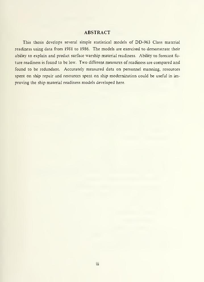
A plot of the shipwide manning level of Chief Petty Officers (E7-E9) reveals some

problems that were not apparent from previous screening of the data. Figure 2 on page

13 shows that some ships had less than 30 percent of required manning of these impor-

tant personnel during a given year-a highly unlikely event. Similar problems are found

in the data values for E4-E6 manning levels. These personnel are less experienced but

also are important in operating and maintaining a ship. Since these data are probably

erroneous, any models using personnel manning levels would be inaccurate.

Development of the model begins following completion of these exploratory' plots.

11

5

. ... * • •

THAT

YD300 ~

* * • *

CLUJcr

• ' •

15 o<-' CM

-*'

* *

u _'

o •

u oUJ o -

*•

DAYS - • •

o 4 1 I.I 1

'1 . 1 1

1000 2000 3000

NUMBER OF REPAIR PARTS ORDERED THAT YEAR

Figure 1. Sample Data Plot: days free of C3 C4 CASREPs as a function of

number of repair parts ordered. A regression line can be imagined from

the upper left to the lower right of the data.

B. ORDINARY LEAST SQUARES REGRESSION

A brief summar\' of terms and methods used in ordinary' least squares regression is

included for clarity.

A statistical routine uses the data to calculate the values of the coefiicients {a) of

the explanatory' variables in the model. The calculated coefficients are those that mini-

mize the sum of the squares of the residuals in the model. Residuals are the difference

between the fitted values (those obtained by inputting the data for each explanatory

variable) and the observed values of the response variable. The calculated coefficients

determine the linear model.

12

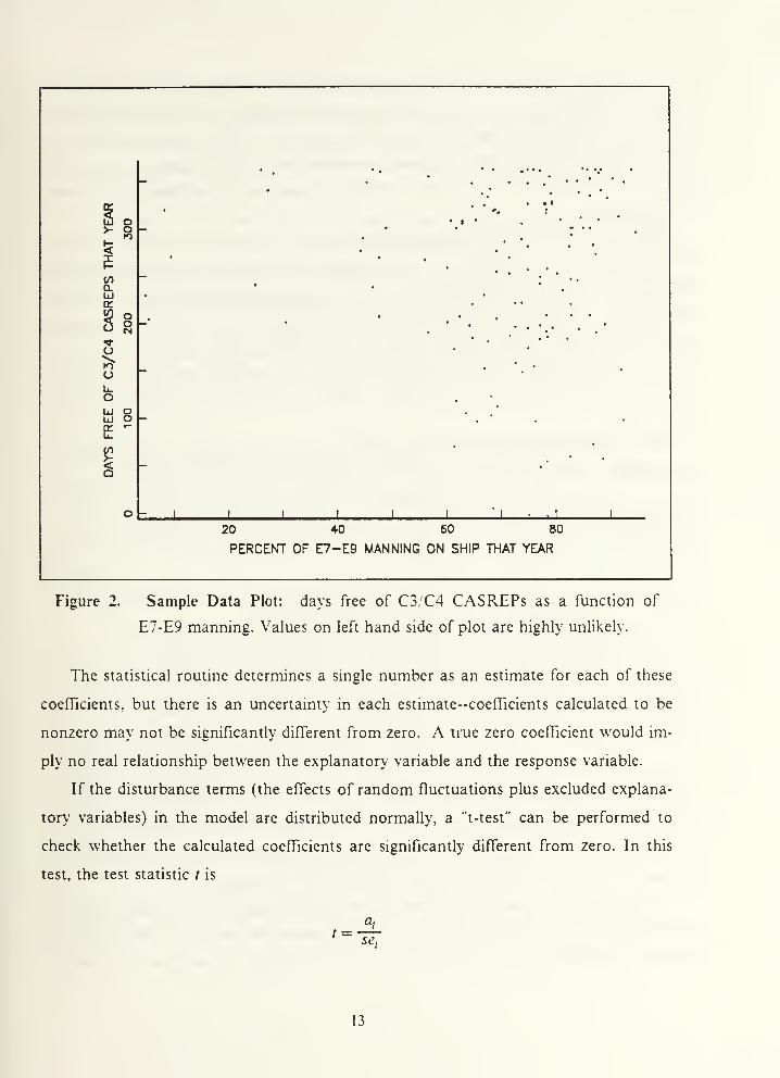
20 40 60 60

PERCENT OF E7-E9 MANNING ON SHIP THAT YEAR

Figure 2. Sample Data Plot: days free of C3,C4 CASREPs as a function of

E7-E9 manning. Values on left hand side of plot are highly unlikely.

The statistical routine determines a single number as an estimate for each of these

coefficients, but there is an uncertainty in each estimate-coefficients calculated to be

nonzero may not be significantly different from zero. A true zero coefficient would im-

ply no real relationship between the explanatory variable and the response variable.

If the disturbance terms (the effects of random fluctuations plus excluded explana-

tory variables) in the model are distributed normally, a "t-test" can be performed to

check whether the calculated coefficients are significantly different from zero. In this

test, the test statistic / is

/ =se;

13

where se, is the standard error (a measure of uncertainty) of the coefficient a,. If the

residuals of the regression are distributed normally, this statistic has the t-distribution,

and the result can be checked for statistical significance. Roughly, if the resulting t-

statistic is greater than two, the coefficient is statistically significant, meaning that there

is less than a five percent chance that a coefficient calculated to be different from zero

is actually zero.

T-tests are of two types: one-sided and two-sided. If the sign of the coefficient is not

known beforehand, a two-sided test is performed; this test simply checks to see if the

coefficient is significantly different from zero. If the sign of the coefficient is known

beforehand, a one-sided test is performed. This test determines if the coefficient is both

significantly different from zero and is also of the correct sign. The procedures for both

tests are almost identical. In the case of the one-sided test, assuming that the calculated

sign is correct, a test statistic of two implies a significance level of about 0.025. [Ref 6:

pp.181-198]

Based on the interpretation of the coefficients as partial derivatives of the explana-

tory' variables, the signs of most coefficients in this model are known beforehand and a

one-sided t-test is used. In the case of the fleet variable, a two-sided t-test is used be-

cause the probable sign of the coefficient for this explanatory variable is not known in

advance.

Throughout the analysis, a significance level of 0.025 is taken to be the minimum

acceptable for including an explanatory variable in the model.

C. DEVELOPING THE PRIMARY MODEL-ITERATIVE APPROACH

Initial computer runs indicate which chosen explanatory' variables are individually

significant in a regression model. For example, percent of time in overhaul is significant

individually, and percent of time in maintenance is "close" to significance, with a t-

statistic of about 1.8. When these variables are placed together as explanatorv' variables

in one model, however, both are insignificant. This is because they contain very similar

information-by definition, time in maintenance includes time in overhaul as well as time

in less extensive maintenance availabilities. This situation is called multicollinearity.

Multicollinear explanatory' variables tend to dilute the significance of a model; therefore,

only one of this family is retained in the model, the time in overhaul.

Another difficulty with this pair of variables is that the signs of their coefficients are

opposite to those expected. The reason for this apparent contradiction is as follows:

when ships go into a major maintenance availability, CASREPs on equipment that will

14

be fixed during the overhaul or maintenance period are usually cancelled at the start of

the maintenance period. Thus more time in overhaul or maintenance is related to more

days free of C3 C4 CASREPs. The greater strength of the time in overhaul variable is

probably due to the fact that overhauls are longer than other maintenance availabilities

and result in more CASREP cancellations.

The number of repair parts ordered is found to be a strong explanatory variable in-

dividually. When it is placed in a model with percent of time in overhaul, the percent

time in overhaul becomes insignificant because of multicollinearity with the number of

repair parts ordered. This relation was previously unsuspected, but makes sense: once in

overhaul, with few ship systems operating and most maintenance work being performed

by shipyard personnel, the crew itself orders few parts. Since number of repair parts is

stronger in explaining days free of CASREPs, it is retained in the model; time in over-

haul is dropped.

When placed in the same model with number of repair parts ordered, all other indi-

vidually significant explanatory variables are insignificant at the 0.025 level. Only one

variable, fleet of ship, is even close to significance, with a t-statistic of about 1.7.

The manning levels of senior enlisted personnel are not significant variables even

when taken individually. This fact is not surprising, based on the apparent problems in

the data.

1. Delayed Effects of Explanaton' Variables

The reversed sign of the time in overhaul variable demonstrates that the appar-

ent short-term effect of an overhaul is to reduce the number of active CASREPs along

with the number of parts requisitions. The next logical step is to look for longer-term

effects of overhauls. The possibility of delayed effects of maintenance had not been

considered in the original model for the sake of simplicity. However, it now appears that

consideration of a time-delayed (lagged) overhaul variable in a new version of the model

is necessarv- to include the CASREP-producing effects of an overhaul. The use of lagged

values of explanatory' or response variables as additional explanatory variables is an ac-

cepted approach in econometrics [Ref 6: pp. 343-371]. Also, a previous study on read-

iness used this approach successfully with explanatory variables [Ref 2 : p. 1/6].

Therefore, the previous year's percent of time in overhaul is entered as an explanatory'

variable for the current year's time free of C3;C4 CASREPs. Results are significant at

the 0.025 level.

15

The successful use of lagged values of an explanator\- variable leads to consid-

eration of lagged values of the response variable itself in the model, since some ship

systems tend to be "lemons", with recurring problems in the same equipment. The sign

of the coefficient is reasoned to be positive, since casuahy-plagued ships tend to remain

in that condition. When the previous year's time free of C3/C4 CASREPs is entered as

an explanatory' variable for the current year's time free of CASREPs, the results are

significant.

Due to the change in requirements for filing CASREPs in 1980, it is necessary

to drop 30 data points in performing this lagging operation, since 1980 CASREPs are

not equivalent to those in later years. This leaves 150 data points for analysis.

2. Consideration of Other Explanatory Variables

At this point, variables not included in the original model are entered into the

regression to see if any might be significant. This is done to find explanatory variables

that might have been overlooked in the model-building stage. It is not expected that any

variables will be significant.

One variable, the manning level of junior enUsted personnel (E1-E3), has a sta-

tistically significant coefficient. This result seems strange, since personnel in these

paygrades are least experienced and least skilled. When the variable is plotted against

the days free of C3 and C4 CASREPs, problems similar to those in senior enlisted

manning levels (see Figure 2 on page 13) are found.

Going back to the original CNA monthly-structured database, the monthly

E1-E3 manning level is plotted against days free of C3;C4 CASREPs in that month (see

Figure 3 on page 17). The data are clearly erroneous-all values are either below 40

percent or above 80 percent, with frequent changes from month to month from below

ten percent to above 90 percent (not discernable from Figure 3 on page 17). Since the

manning level on a ship never fluctuates in this way, it is clear that there is a major error

in this variable, and it was by chance that junior enUsted manning level is statistically

significant. This variable is not used in any model.

Based on these observations, it appears that the personnel manning level data

in the CNA database are erroneous. Although this study is unable to use these data on

personnel manning, accurate personnel data could be significant explanatory" variables

for ship material readiness.

16

Ob

R -:

o..

H.:•

•

V) OOl cmUJtr

. .

•

^P

-"

o•

fe° -

.

bJbJ

.

i

^. •

I. I _L _L _L

20 40 60 BO

PERCENT OF E1-E3 MANNING ON SHIP THAT MONTH

TOO

Figure 3. Personnel Data Problems: days free of C3C4 CASREPs versus El -E3

manning. Data for three of 30 ships in the study are shown.

3. Consideration cf Data Transformations

Transformations of the data are not used because the data are not distributed

in a way lending to improvement in results from transformations.

4. VAMOSC Data

Once the VAMOSC data are available, exploratory' data analysis similar to that

conducted on the CNA data is performed. No problems are found.

Fiscal variables of interest are then put into the regression program, as indicated

by asterisks in the Appendix. The VAMOSC data are scaled from dollars into thousands

of dollars to keep the coefficients of the model of the same order of magnitude as those

obtained using the CNA data. This approach prevents possible numerical problems in

17

software being used. Only two variables have significant coefficients: Technical Avail-

abilityl (TAV) labor and TAV material. These variables were initially projected to have

negative coefficients because more maintenance is related to more CASREPs, as dis-

cussed above. TAV labor enters the model with a negative coefficient, but the calculated

coefficient for TAV material is positive, indicating that more maintenance is related to

fewer CASREPs. This problem requires further investigation.

5. Initial Model Results

The initial results of the primar>' model using all five significant explanatory

variables are

>'i= c, + a^x^ + a2X2 + a^x^ + a^x^ -\- a^x^

where

;-, =days free of C3 and C4 CASREPs, in days (on a yearly basis)

c, =constant or intercept in days

x^ =number of repair parts ordered, in units

.x^ =previous year's days free of C3 and C4 CASREPs, in days

jCj =percent of time in overhaul during the previous year, in percent

Xi =money spent for labor in technical availabilities, in thousands of 1986 dollars

jfj =money spent for material in technical availabilities, in thousands of 1986 dollars

Note that the x, here are not the same as those proposed in the original primar\'

model. The a, here are the fitted coefficients of the linear model based on calculations

using the data. Their values are listed in Table 1 on page 19 along with the other nu-

merical values of interest for the model at this stage.

R' is the proportion of the total variation in the response variable explained by

the regression model. The standard error of the regression is a measure of the variability

of the results of the model. Smaller standard errors imply more precision in the model.

1 A Technical Availability is an unscheduled maintenance availability that does not prevent

the ship from earning out its mission.

18

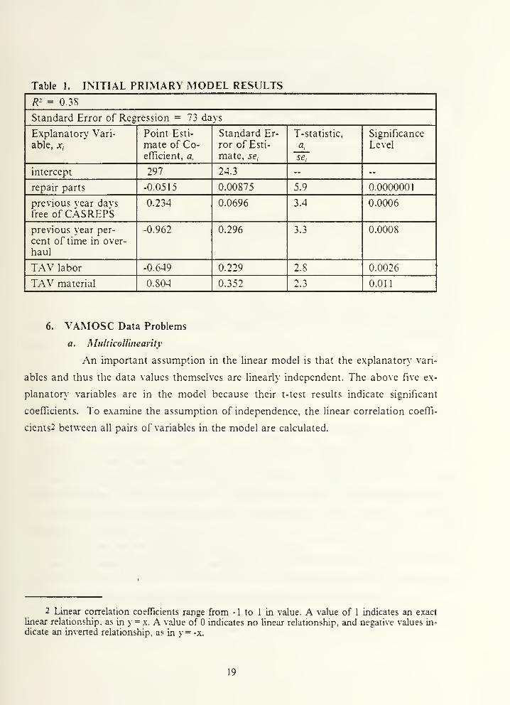
Table 1. INITIAL PRIMARY MODEL RESULTS

/?- = 0.38

Standard Error of Regression = 73 days

Explanatory- Vari-

able, jr,

Point Esti-

mate of Co-efficient, a,

Standard Er-

ror of Esti-

mate, se,

T-statistic,

5^,

Significance

Level

intercept 297 24.3 " --

repair parts -0.0515 0.00875 5.9 0.0000001

previous vear davs

free of CASRE PS0.234 0.0696 3.4 0.0006

previous year per-

cent of time in over-

haul

-0.962 0.296 3.3 0.0008

TAV labor -0.649 0.229 2.8 0.0026

TAV material 0.804 0.352 2.3 0.011

6. VAMOSC Data Problems

a. Multicollineaiity

An important assumption in the hnear model is that the explanaton.' vari-

ables and thus the data values themselves are linearly independent. The above five ex-

planatory" variables are in the model because their t-test results indicate significant

coefficients. To examine the assumption of independence, the linear correlation coefii-

cients2 between all pairs of variables in the model are calculated.

2 Linear correlation coefficients range from -1 to 1 in value. A value of 1 indicates an exact

linear relationship, as in y = x. A vaJue of indicates no linear relationship, and negative values in-

dicate an inverted relationship, as in y= -x.

19

Table 2. LINEAR CORRELATION COEFFICIENTS

Variable, x, repair

parts

or-

dered

previous

year days

free of

CASREPs

previous

year

percent

time in

overhaul

TAVlabor

TAVmaterial

davs free

of'

CASREPs,

repair parts

ordered

1

previous

year daysfree ofCASREPs

-0.28 1

previous

year percent

time in over-

haul

0.07 0.30 1

TAV labor 0.13 -0.01 0.19 1

TAV mate-rial

0.11 -0.02 0.17 0.92 1

davs free of

CASREPs,Vi

-0.51 0.2S -0.21 -0.22 -0.15 1

Table 2 shows the high linear correlation between the TAV labor and TAV

material explanatory' variables. It is then necessary- to determine the effect of keeping

these variables in the model, because the multicollinearity could explain the unantic-

ipated sign of the TAV material coefficient.

A small side study is performed in which each of the two TAV variables is

used as the response variable in a regression using repair parts ordered, lagged overhaul

time and lagged lime free of CASREPs as explanatory variables. In each case, the R^ is

insignificant (about 0.04), and the residuals of these two regressions are highly correlated

(linear correlation coefficient of 0.92). Therefore, it is believed that the simple correlation

coefficient of these two TAV variables (0.92 as listed in Table 2) would not be notice-

ably altered in the presence of the other explanatory variables; the redundant informa-

tion contained would not be reduced.

In examining this problem further, each of the two TAV variables is sepa-

rately entered into the regression package as an explanatory* variable along with the

previous three explanatory' variables (repair parts ordered, lagged overhaul time and

20

lagged time free of CASREPs) to observe its performance with time free of CASREPs

being the response variable. Results are listed in Table 3 on page 21. TAV labor alone

again has the expected negative coefficient, but the significance of the result is diluted

to less than 0.025. When TAV material is entered into the regression package without

labor, its regression coefficient is not significantly different from zero at the 0.025 level.

Table 3. MULTICOLLINEARITY EFFECTS ON REGRESSION RESULTS

TAV Variable Coefficient Stand. Error T-statistic Significance

labor

material

(taken together)

-0.649

0.804

0.229

0.352

2.8

2.3

0.0026

0.011

labor, alone -0.168 0.093 1.8 0.033

material, alone -0.101 0.14 0.77 0.22

labor plus material -0.0S28 0.058 1.4 0.074

Note that when TAV labor and material are placed together in a model,

they have an offsetting effect; their coefficients are of the same magnitude but are op-

posite in sign.

Inclusion of multicollinear variables in a regression model often increases

the standard errors of the affected variables. This results in unstable coefTicient estimates

and reduces the significance of t-tests conducted, frequently making the explanatory'

variables insignificant. This had been the case for all previous related variables observed

in the study. However, with the TAV labor and TAV material variables, in spite of the

relatively large standard errors and unstable coefTicients, the results of t-tests are still

significant. It should be noted that throughout this exercise of checking for

multicollinearity, the estimates of coefficients and standard errors for each of the other

three explanatorv' variables in the model remain almost constant. Based on the above

it is decided to drop the VAMOSC variables from the model. Further support for this

action is discussed below.

b. Checking for Stability

The effect of running the model with certain data points excluded is exam-

ined next. In the case of the TAV labor and TAV material variables, certain data points

are relatively far from other data points. These isolated points are known as "high lev-

erage points" [Ref 7: pp. 249-255] because a single point can have a disproportionate

effect on the outcome of the repression model.

21

»• %

4. .

"

f.•

.

K1 ' ' ••

U O I._ .

>- o -—

K1 t

h- *'•

< ,'

f '•

</1-?

Q. *.^

Id • •

tr .• . -

S? o • *•• •

f\ o " * •^ CM •

't .• •o • •\n ^ '

u •

b.O ;

Ld O •

UJ O —', ^

E-

^/

< —' ,

Q

O -i 1 1 1- 1 1

200 400 600

TAV U\BOR IN THOUSANDS OF DOLU\RS

Figure 4. Illustration of High Leverage Points

In Figure 4 on page 22, the placement of a line fitted to the data can vary

considerably if any or all of the five rightmost data points are excluded from consider-

ation. Also, the large number of zero values in this data can tend to throw off the re-

gression solution. None of these data values was clearly wrong or miscopied, but there

could be strong effects on the resulting model.

Accordingly, regressions are run again, this time dropping one point at a

time on the extreme right of Figure 4, with five points fmally being dropped. Estimates

of coefficients and standard errors var>' considerably. T-test results are inconsistent—

sometimes the t-test statistic degrades and sometimes it improves. Some of this effect is

undoubtedlv related to the multicollinearitv of the TAV variables.

22

Combined with the results of the multicoUinearity investigation, this exer-

cise results in dropping both the TAV labor and TAV material explanatory* variables

from the model.

The other three explanator>' variables have no isolated points, due in part

to the bounded nature of the lagged values of days free ofCASREPs and percent of time

in overhaul.

D. INTERMEDIATE PRIMARY MODELWhen these two VAMOSC explanatory variables are dropped, the model is

where

y^ =days free of C3 and C4 CASREPs (on a yearly basis)

c, =constant or intercept, in days

jCj =number of repair parts ordered, in parts

jr2 =previous years days free of C3 and C4 CASREPs, in days

jTj =percent of time in overhaul during the previous year, in percent

Numerical values of interest for this model are listed in Table 4. Note the similari-

ties in this iteration of the priman." model to the initial primar\- model listed in Table 1

on page 19. The exclusion of the TAV variables has little effect on the model, and R- is

reduced only slightly, from 0.3S to 0.34.

Table 4. INTERMEDIATE PRIMARY MODEL RESULTS

R- = 0.34

Standard Error of Regression = 75 days

Explanatory- Vari-

able, Xi

Point Esti-

mate of Co-efiicient. a,

Standard Er-

ror of Esti-

mate

T-statistic Significance

intercept 297 24.9 " --

repair parts -0.0535 0.00891 6.0 0.00000008

previous year davs

free of CASREPs0.233 0.0710 3.3 0.0007

previous year per-

cent time in overhaul

-1.06 0.297 3.6 0.0003

23

o«o - *

K1 •

en"

•

D.UJ ^ •

K.

•

O O•

CM — • -•^ K)

U "

\no —,

u. .

O ,

o •

UJ CO —UJ (Mcru. •

^-

<Qic ?K) SC75 •

_l<Z)

§8CNJ

1 I.I 1 1 1

280 320 360

niTED DAYS FREE OF C3/C4 CASREPS

Figure Demonstration of Primar}' Model: plot of actual days free of C3 C4

CASREPs in 1986 against days free of CASREPs fitted by primary

model using 1986 data

This model provides "fitted" values of the days free of C3 and C4 CASREPs based

on the values of the explanatory variables, and these values can be compared with the

actual observed days free of C3'C4 CASREPs. Figure 5 on page 24 displays the use of

1986 data for the explanatory variables in exercising the model. Fitted values came

within one standard error (75 days) of the actual value of the response variable for 25

of the 30 ships. The maximum difference between fitted and actual values was 1.6

standard errors, or 106 days.

Though this model is useful for explaining readiness and removes about one third

of the variation in material readiness, it is not able to predict the material readiness of

a ship for the upcoming year, because one of the explanaton.' variables (number of repair

24

parts ordered) cannot be controlled and is not known until the upcoming year is over.

A lagged repair parts ordered variable is not significant in the t-test, so the efiect of re-

pair parts cannot be included in a predictive model.

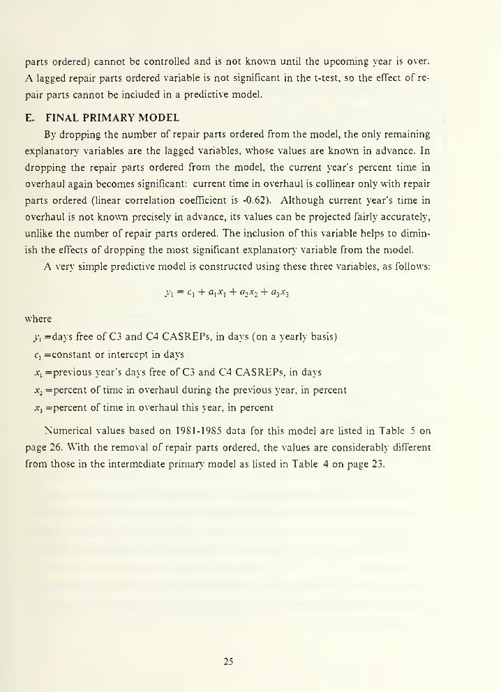
E. FINAL PRIMARY MODELBy dropping the number of repair parts ordered from the model, the only remaining

explanatory variables are the lagged variables, whose values are known in advance. In

dropping the repair parts ordered from the model, the current year's percent time in

overhaul again becomes significant: current time in overhaul is collinear only with repair

parts ordered (linear correlation coefficient is -0.62). Although current year's time in

overhaul is not knowTi precisely in advance, its values can be projected fairly accurately,

unlike the number of repair parts ordered. The inclusion of this variable helps to dimin-

ish the effects of dropping the most significant explanatory' variable from the model.

A ven.- simple predictive model is constructed using these three variables, as follows:

ji'j = C] + a,JCj + a2A-2 + 03X3

where

j'l =days free of C3 and C4 CASREPs, in days (on a yearly basis)

c, =constant or intercept in days

jc, =previous year's days free of C3 and C4 CASREPs, in days

X2 =percent of time in overhaul during the previous year, in percent

x^ =percent of time in overhaul this year, in percent

Numerical values based on 1981-1985 data for this model are listed in Table 5 on

page 26. With the removal of repair parts ordered, the values are considerably different

from those in the intermediate primar\' model as listed in Table 4 on page 23.

25

Table 5. PRIMARY PREDICTION MODEL RESULTS

R' = 0.23

Standard Error of Regression = 81 days

Explanatory- Vari-

able, X,

Point Esti-

mate of Co-efficient, a,

Standard Er-

ror of Esti-

mate

T-statistic Significance

intercept 186 18.0 " "

previous vear davs

freeofCASREPS0.323 0.0744 4.3 0.00003

previous year per-

cent time in overhaul

-1.33 0.317 4.2 0.00004

percent of time in

overhaul this year

0.897 0.292 3.1 0.0014

To avoid bias in predicting days free of CASREPs in 1986, this model is calculated

using only the 120 data points from 1981 to 1985. The differences between this predictive

model and the previous intermediate model are due mainly to the different explanaton.'

variables, not to the fewer data points used.

The price of exchanging the most significant explanator\' variable for a less signif-

icant one is evident. This model explained less than a fourth of the variation in the days

free of C3 C4 CASREPs, and it had a larger standard error. The low R^ of this model

reflects a poor ability to predict future readiness of individual ships.

To demonstrate the use of this model, the 1985 data (with 1986 values for time in

overhaul) are used to forecast the days free of C3;C4 CASREPs for each ship in 1986.

Results are shown in Figure 6 on page 27.

In 14 of the 30 ships, the prediction model is able to forecast within plus or minus

60 days the number of days free of C3,C4 CASREPs. In 20 of the 30 ships, predictions

are within plus or minus 90 days of the actual values. With the larger standard error in

this model (81 days), 20 of the 30 predictions are within plus or minus one standard error

of the actual value.

It can be seen that the predictions are conservative, although conservatism is not a

design characteristic of the model. Actual days free of C3;C4 CASREPs are generally

better than those predicted.

26

o • • •

(O mm •

KJ

• •

w .

Q.~

UJ ^• "

o:

!§ o?i *^ — •

t) K)^

•* •

y> -,

o "

FREE 280 -•

10•

>-< ~Q(OCO o21 s_J<13 —1-u< oo —

P>J

11 1 1 1

1 . 1

200 240 280

PREDICTED DAYS FREE C3/C4- CASREPS

Figure 6. Demonstration of Primar}' Prediction Model: plot of actual days free

of C3 C4 CASREPs in 1986 against days free of CASREPs fitted by

priman.- prediction model using 1985 data, with 1986 values for current

year's time in overhaul.

F. EXAMINATION OF ASSUMPTIONS

Several assumptions are necessar}' in order to perform ordinary least squares re-

gression. It is necessary to check that these assumptions are met in order to use such a

model. The assumptions are:

• explanatory variables are fixed

• explanatory variables are linearly independent

• residuals are distributed normally with mean zero

• residuals are homoscedastic (have constant variance with respect to explanator>'

variables and ships) and are not autocorrelated

27

The first assumption is based on popular utilization of multiple linear regression

methods. The explanatory' variables span their ranges well and results of the analysis are

conditional, given the value of the explanatory' variables.

The assumption of linear independence of explanatory variables is validated by the

previous checks for multicollinearity.

To check the assumption of normal disturbances, a Kolmogorov-Smirnov test of the

residuals [Ref 8: pp. 552-559] is performed by the GRAFSTAT package. An adjustment

is necessary due to the necessity of estimating the sample variance of the hypothesized

normal distribution. Stephens' method [Ref 9] is used, and a significance level of 0.10 is

obtained. Based on this result, it is decided that the assumption of normal distribution

of residuals is reasonable. This is a prerequisite for meaningful tests of hypotheses

concerning the coefficients of the regression.

To check the last assumption of constant variance with no autocorrelation, the res-

iduals of the regression are plotted against each explanatory' variable. Residuals for each

of the 30 ships are plotted as a function of time, and Durbin-Watson statistics (Ref 6:

pp. 314-317], which are a measure of autocorrelation, are computed for each ship. Ide-

ally, all of these tests should show that the residuals of the regression have no pattern,

indicating good adherence to the last assumption of the model. Plots involving residuals

from all 30 ships show no structure, but when each ship is examined individually, prob-

lems arise. Autocorrelation of ship residuals (meaning that a ship's residuals are related

to its residuals from previous years) and heteroscedasticity (difierences in the variabihty

of one ship's residuals as compared to another ship's) are both apparent.

It is necessan.' to investigate the effect of not meeting the assumption of

homscedasticity and no autocorrelation.

I. Checking for Structural Change

The first step in this process is to check the data to ensure they are "uniform"

in the sense that there was no change in the underlying process causing CASREPs dur-

ing the time period of the data. The statistical test for structural change [Ref 6: pp.

207-211] involves taking time subsets of the database, performing regressions on these

subsets, and determining whether the model coefficients from each subset are signif-

icantly different. The data are divided into subsets of 1981-1983 and 1984-1986, and the

test finds no evidence of structural chanee over these subsets.

28

2. Transformed Model

With no structural change in the database, a data transformation specifically

designed to correct for autocorrelation and heteroscedasticity is found in the literature

[Ref. 10: pp. 616-620]. This transformation uses the information contained in the data

to correct these problems. The transformation is nonlinear and has two stages: the first

stage removes the time correlation of the residuals of the regression model and the sec-

ond stage removes the effects of the differing variability among the ships. The transfor-

mation exploits all the information available in the data to obtain the most efficient

estimators of the primary prediction model.

A brief explanation of the transformation is as follows:

• each ship's residuals from the primary prediction model are used to determine an

individual ship autocorrelation parameter

• using this parameter, the response and explanatory data for each ship undergo a

first-order autoregressive transformation

• a second ordinar\' least squares regression is performed on these transformed data.

The residuals from this regression are less autocorrelated, and they are used to es-

timate the individual sample variance in the time free of CASREPs for each ship.

• using the sample variance computed for each ship, the data undergo a second

transformation to remove the inherent heteroscedasticity.

• a final ordinary least squares regression is now run on the twice-transformed data

When the transformed model is run, the value of R^ obtained is 0.72, a large

improvement over the 0.23 value of i?^ for the primary' prediction model. But because the

variables in the transformed model have no physical meaning, a direct comparison of

these statistics is not valid. The transformed model can be used to predict future values

of readiness only after its results are retransformed back into the original units of days

free of C3 C4 CASREPs. When this is done, there is more variation in the transformed

model than in the final primar}' prediction model. See Figure 7 on page 30 for a display

of these predictions, and compare to Figure 6 on page 27. Nine of the 30 predicted

readiness values are greater than 365 days free ofCASREPs when transformed back into

original units, with one forecast of 1100 days free of CASREPs.

The assumptions of homoscedasticity and no autocorrelation are satisfied by the

transformed model better than by the original primary model, but the transformed model

is not practical due to the increased variability of its forecasts. Some of this is probably

due to the short time span of the database.

29

o

V)

cr

-.

•.

55 o - ••

-•

• •

FREE 280 -•

i-

1986 240 -

ACTUAL

200

1 1 1 1 1 1 I.I 1

150 200 250 300 350

PREDICTED 1986 DAYS FREE C3/C4 CASREPS

Figure 7. Results of Retransformation: plot of predicted 1986 days free of

CASREPs and actual 1986 days free of CASREPs produced by

retransforming the values from the transformed model back into units

with physical meaning. Predicted values greater than 365 days free of

CASREPs are truncated to 365.

This excursion to better satisfy the model assumptions of no autocorrelation

and homoscedasticity is not helpful. It appears that the primar>' prediction model is

more useful in predicting material readiness despite its auiocorrelated and

heteroscedastic characteristics.

30

V. ANALYSIS OF ALTERNATE MODEL

The analysis of the alternate readiness model is ver>' similar to that of the primar\'

model. Since the same databases are used for the explanatory- variables, the only new-

exploratory' data analysis necessary is for the response variable, C3;C4 CASREP-days.

No problems are noted, but it is obvious that this measure of readiness is more variable

than days free of C3/C4 CASREPs.

Once ordinary least squares models are run, results are remarkably parallel to those

of the primary model. The same explanatory variables are consistently found to be sig-

nificant in both of the models. The effects of the multicoUinearity of TAV labor and

TAV material variables are virtually identical. Investigation of possible high leverage

points has the same results.

The reason for these similarities is found in a simple plot of the primary- measure of

readiness against the alternate measure, as seen in Figure 8 on page 32. Except for a feu-

data points that represent ships with "bad" years for C3 and C4 CASREPs, the two

measures of readiness are closely related. The linear correlation coefficient between the

two measures of readiness is -0.82, indicating a strong, inverted linear relation.

This plot suggests further investigation into the relation between the two measures

of readiness. It is then noted that the sum of days free of CASREPs and C3/C4

CASREP-days during a year is frequently 365; in other words, there is often either zero

or one C3 or C4 CASREP at a time on many ships. Thus the alternate measure of

readiness is rendered redundant: the original idea of having a second measure of material

readiness that is sensitive to multiple ongoing C3 and C4 CASREPs is defeated.

For consistency, lagged values of the alternate readiness measure are used as ex-

planatory variables in the alternate model, just as lagged values of the primary readiness

measure are used in the primary model.

The results of the alternate model using all three significant explanatory variables

are

y2 = C2 + b^X] + b2x'2 + bjXj

where

>'2 =C3 and C4 CASREP-days, in CASREP-days (on a yearly basis)

C2 =constant or intercept, in CASREP-days

31

\

-IV/

^ V^ 1 .

Ld O k *• •

>- o -m •

fO 1

K •"

/ t

pE'••

«

</1- *•.*•,

a. ;•

u •

d: *• • •

55 o .. • • •

S o — • ^ /*J CM •,. ^ • •

^ " • ' •

o •

\n ,•

o '

b.o .

UJ o •

UJ o —.

'• •

e^

^ ^

'

< _ ',

D

o H 1 1 . 1 1 1 .1 1

4-00 BOO 1200 1600

C3/C4 CASREP-DAYS THAT YEAR

Figure 8. Relation bet^veen Priman and Alternate Readiness Measures

jr, =number of repair parts ordered, in parts

x'2 =previous year's C3 and C4 CASREP-days, in CASREP-days

JC3 =percent of time in overhaul during the previous year, in percent

b, =fitted coefTicients calculated from the data

Numerical results for this model are in Table 6 on page 33. This model corresponds

to the intermediate primary model listed in Table 4 on page 23. Note the large difference

in the standard error of the regression.

32

Table 6. INTERMEDIATE ALTERNATE MODEL RESULTS

R' = 0.31

Standard Error of Regression = 181 days

Explanatorv Vari-

able

Point Esti-

mateStandard Er-

ror of Esti-

mate

T-statistic Significance

intercept -68.7 35.7 " --

repair parts ordered 0.105 0.00214 4.8 0.00005

lassed C3, C4CASREP-days

0.257 0.0594 4.4 0.00003

lagged percent time

in overhaul

2.06 0.700 2.9 0.0023

The numerical measure of the ability of the model to explain C3 and C4

CASREP-days, /?^ is very close to that for the primary intermediate model. The signs

of the coefTicients are as expected: opposite those of the primary model for parts ordered

and percent time in overhaul, and the same for the lagged response variable.

This model is then used to compare the fitted values of C3;C4 CASREP-days for

1986 to the observed values for that year. For the 30 ships in the class, 16 of the fitted

values are within plus or minus 60 CASREP-days of the actual values, and 21 fitted

values are within plus or minus 90 CASREP-days of the actual values. The precision of

the alternate model appears less than that of the primar\' model because of the un-

bounded nature of the alternate measure of readiness and the resulting greater variabil-

ity. With the standard error of the regression of 181 C3,'C4 CASREP-days, 28 of the 30

fitted values are within plus or minus one standard error of the actual values.

A. ALTERNATE PREDICTION MODELOnce again, as in the primary model, the number of repair parts ordered is dropped

from the model in order to make a predictive model. Here, the current year's percent

time in overhaul is not included in the final alternate prediction model since, strictly

speaking, it is not known in advance. The exclusion of this explanatory variable makes

little difference in the model or in its ability to predict readiness in the upcoming year.

33

This model again uses the 1981-1985 data, 120 data points, in order to avoid bias in

predicting values for 1986 C3'C4 CASREP-days. The coefficients and statistics of in-

terest for this prediction model are shown in Table 7, and the model is demonstrated in

Figure 9 on page 35.

Table 7. ALTERNATE PREDICTION MODEL RESULTS

R' = 0.20

Standard Error of Regression = 208 days

Explanatorv' Van-able

Point Esti-

mateStandard Er-

ror of Esti-

mate

T-statistic Significance

mtercept 80.0 28.8 - "

laooed C3 C4CASREP-days

0.316 0.0685 4.6 0.00002

lagged percent time

in overhaul

3.48 0.91S 3.8 0.0002

Once again, the model loses some of its ability to explain the variation in C3;C4

CASREP-days in the tradeoff to be able to forecast future values of readiness. Pred-

ictions for 24 of the 30 ships are within one standard error of the actual CASREP-days.

The standard error itself, however, is 208 days, indicating the loss of precision due to the

greater variability of the alternate measure of readiness as compared with the primar>'

measure. Ten of the 30 predictions are within plus or minus 60 CASREP-days of the

actual values, and 17 of the 30 are within plus or minus 90 CASREP-days of actual.

Due to the close relationship between the primar}' and alternate measures of read-

iness, the alternate model has the same difficulties as the primarv' model with the as-

sumptions of no autocorrelation and homoscedasticity of residuals. Data transformation

of the alternate model has the same effect and shortcomings as those discussed for the

primarv' model.

34

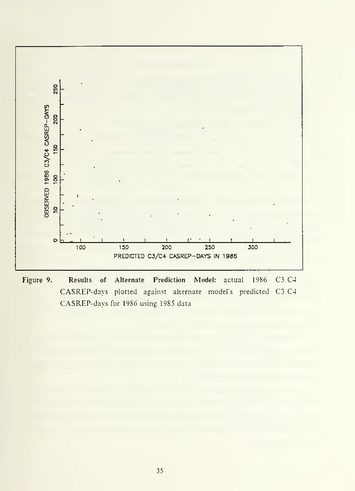
100 1 50 200 250

PREDICTED C3/C4 CASREP-DAYS IN 1985

300

Figure 9. Results of Alternate Prediction Model: actual 1986 C3 C4

CASREP-days plotted against alternate model's predicted C3 C4

CASREP-days for 1986 using 1985 data

35

VI. CONCLUSIONS

It is important to note that the explanatory variables found to be significant in their

relation to readiness do not cause ship readiness to behave as it does; rather they are

merely related to readiness.

A. COMPARISON OF MEASURES OF READINESS

The alternate measure of readiness, C3 and C4 CASREP-days, is not significantly

better in any apparent way than the primar\- OP-81 measure, time fi-ee ofCS and C4

CASREPs. The two are ver\" closely related in this data set: since most ships have at

most one C3 or C4 CASREP at a time, the two measures of readiness are simply alter

egos.

This fact does not prevent the alternate measure of readiness from being useful in

different circumstances-perhaps with a different set of ships at a different time, there

could be enough simultaneous C3 and C4 CASREPs to create a significant difierence in

the two measures of readiness.

B. USEFUL EXPLANATORY VARIABLES

It is considerably easier to provide a fitted value for a past or current year's material

readiness than to predict next year's material readiness for a ship. This fact is true for

both measures of readmess. The most useful variables found by this study are repair

parts ordered, previous year's readiness and previous year's time in overhaul. All three

of these variables are easy to explain and collect data on.

Unfortunately, none of the VAMOSC variables can be used in predicting material

readiness. It appears that the fiscal explanatory' variables in the VAMOSC database are

not sufficiently focused to be helpful. Due to this, the models developed are not useful

for programming maintenance funding.

It would be helpful to discriminate between maintenance funds spent for repairing

existing material problems and those funds spent for modernization and overhaul of

older systems-this would enable associating each of these variables with the appropriate

effect of CASREP termination (repair activities) or CASREP generation (overhaul'

modernization activity).

36

C. DATA COLLECTION

As discussed above, collecting separate data on funds spent to repair ships and funds

spent to upgrade and overhaul them would be helpful.

Additionally, collecting more accurate data on personnel manning and turnover in

the senior enlisted ranks (E4-E6 and E7-E9) among the Combat Systems and Engineer-

ing ratings could lead to good improvements in readiness models. Moreover, turnover

and manning data can be projected into the future (similarly to time in overhaul), giving

an ability to predict their future effect on maintenance, even when exact dates for per-

sonnel detaching and reporting are not known in advance.

D. GENERAL CONCLUSIONS

The models of ship readiness developed in this thesis do not succeed in their goal

of assisting in the programming of Navy funds. Fiscal data available for the study are

not sufficiently focused to be helpful in explaining ship readiness. The resulting models

are capable of modest predictions of future ship readiness, but such predictions are not

necessarily useful. It would be dangerous to avoid overhauls simply because they led to

later C3 and C4 CASREPs: overhauls and modernization of our ships are required to

keep them effective. The simplicity of the models developed here is helpful for some in-

sight into ship material readiness and factors related to it, but the models are not helpful

for planning budgets.

37

APPENDIX DESCRIPTION OF VARIABLES

The following is a listing of all of the explanatory' variables involved in the study.

Variables used in the model are denoted by an asterisk.

VAMOSC DATAThe hierarchical structure of the VAMOSC data set is reflected by the indentations

below. The leftmost variables were aggregated by summing the variables beneath themand to the right. Units are dollars unless otherwise indicated.

Direct Unit Costs

Total Personnel

ManpowerOrganizational Maintenance Labor Manhours *

Officer ManpowerEnlisted Manpower

Temporary Additional Duty of CrewMaterial

Ship Petroleum. Oil, and Lubricants (POL)Total Fuel

Fuel UnderwayFuel Not Underway

Other POLBarrels of Fuel Consumed

Barrels Consumed UnderwayBarrels Consumed Not Undenvay

Repair Parts

Supplies

Equipment and EquipageConsumablesShip Force Material *

Training Expendable Stores

AmmunitionOther Expendables

Repairables

Organizational ExchangesOrganizational Issues

Purchased Services

Direct Intermediate Maintenance Costs

Afloat Maintenance Labor *

Ashore Maintenance Labor *

Material *

Afloat Repair Parts *

Ashore Repair Parts *

Commercial Industrial Services

38

Direct Depot-Level Maintenance Costs

Scheduled Ship OverhaulRegular Overhaul (ROH)

Public Shipyard ROHOverheadLabor *

Labor Mandays *

Material *

Private Shipyard ROH *

Ship Repair Facility ROHOverheadLabor *

Material *

ROH CompletionSelected Restricted Availabihty (SRA)

Public Shipyard SRAOverheadLabor *

Labor Mandays *

Material *

Private Shipyard SRA *

Ship Repair Facility SRAOverheadLabor '^"

Labor Mandays *

Material *

Unscheduled Ship Repair

Restricted Availabilities (RAV)Public Shipyard R.^V

0\erheadLabor *

Labor Mandays *

Material *

Private Shipyard RAV *

Ship Repair Facility RAVOverheadLabor *

Material *

Technical Availabilities (TAV)Pubhc Shipyard TAV

OverheadLabor *

Labor Mandays *

Material *

Private Shipyard TAV *

Ship Repair Facility TAVOverheadLabor *

Material *

39

Fleet Modernization Program (FMP) *

Public Shipyard FMP *

Special Program Material *

Other FMPOutfitting and Spares

Other Depot Costs

Naval Aviation Depot *

OverheadLabor *

Material *

Field Change Installation *

Rework *

Ordnance Rework *

Hull, Mechanical and Electrical Rework *

Electronics Rework *

Design Services Allocation

CNA DATAManning levels are available relative to mobilization requirements and as raw counts

of personnel.

Ship Activities

Percent of Time DeployedPercent of Time Deployed to Fon^'ard Areas *

Percent of Time in Maintenance *

Percent of Time in Overhaul'•'"

Percent of Time Gone from Homeport more than two monthsPercent of Time Inport

"

Percent of Time UnderwayHours Steaming UnderwayHours Steaming Not Underway *

Age of Ship"

Time Since Overhaul *

Time Since Deployment *

Time Since Departed on Deployment *

INSURV Inspection HeldPercent of Preventive Maintenance Items Performed *

INSURV Material Condition Index *

Change of Command HeldFleet (Pacific or Atlantic Homeport) *

Training Inspections HeldParticipation in Joint or Major Exercises

Commanding Officer Information

Relative Seniority of COCO Previous Experience as CO, Executive Officer, or Department HeadTime as CO of this Ship

40

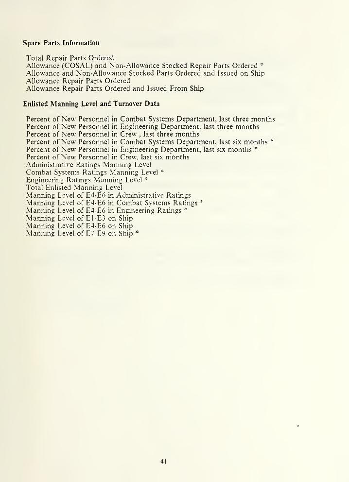
Spare Parts Information

Total Repair Parts OrderedAllowance (COSAL) and Non-Allowance Stocked Repair Parts Ordered *

Allowance and Non-Allowance Stocked Parts Ordered and Issued on Ship

Allowance Repair Parts OrderedAllowance Repair Parts Ordered and Issued From Ship

Enlisted Manning Level and Turnover Data

Percent of New Personnel in Combat Systems Department, last three monthsPercent of New Personnel in Engineering Department, last three monthsPercent of New Personnel in Crew , last three monthsPercent of New Personnel in Combat Systems Department, last six months *

Percent of New Personnel in Engineering Department, last six months *

Percent of New Personnel in Crew, last six monthsAdministrative Ratings Manning Level

Combat Systems Ratings Manning Level *

Engineering Ratings Manning Level *

Total Enlisted Manning Level

Manning Level of E4-E6 in Administrative Ratings

Manning Level of E4-E6 in Combat Systems Ratings *

Manning Level of E4-E6 in Engineering Ratings *

Manning Level of E1-E3 on Ship

Manning Level of E4-E6 on ShipManning Level of E7-E9 on Ship *

41

LIST OF REFERENCES

1. Johns Hopkins University Applied Physics Laboratorv' Technical Report,Relationships Between Resources and Readiness for Surface Combatants, by R.

Freeman, March 1986.

2. MATHTECH, Incorporated Technical Report, A Model to Program MaintenanceResources for Ship Readiness: A Final Report (U), bv E. Feldman and others, April1987. (SECRET Document)

3. Center for Naval Analyses Research Memorandum 86-123, OPTEMPO and Ship

Readiness, by L. Cavalluzzo, D. Follmann, and A. Marcus, June 1986.

4. Center for Naval Analyses Research Memorandum 86-178, Ship EmploymentHistories and Their Use, by K. Domabyl and P. Reslock, July 1986.

5. Center for Naval Analyses Research Memorandum 87-36, The Effect of a Ship's

Employment History on the Material Condition Index, by D. Follmann, April 1987.

6. Johnston, J., Econometric Methods, third edition, McGraw-Hill Book Companv,I9S4.

7. Chambers, J. M., and others. Graphical Methods for Data Analysis, Duxburv Press,

1983.

8. Degroot, M. H.. Probability and Statistics, second edition, Addison WesleyPublishing Company, 1986.

9. Stephens, M. A., "EDF Statistics for Goodness of Fit and Some Comparisons."Journal of the American Statistical Association, v. 69, pp. 730-737, September 1974.

10. Kmenta. J., Elements of Econometrics, second edition, Macmillan Publishing

Company, 1986.

42

INITIAL DISTRIBUTION LIST

No. Copies

1. Defense Technical Information Center 2

Cameron Station

Alexandria, VA 22304-6145

2. Library', Code 0142 2

Naval Postgraduate School

Monterey, CA 93943-5002

3. Chief of Naval Operations (OP-8 14) 1

Attn: CDR Butt

Navy DepartmentWashington, DC 20350-2000

4. Commander, Naval Sea Systems Command (SEA 017EV) 1

Attn: Mr. WebbNaval Sea Svstems Command HeadquartersWashmgton,' DC 20362-5101

5. Center for Naval Analyses 1

Attn: Dr. Quester4401 Ford AvenuePost Office Box 16268

Alexandria, VA 22302

6. Superintendent 1

Attn: Prof. Boger (Code 54Bo)Naval Postgraduate SchoolMonterey, CA 93943-5100

7. Superintendent 1

Attn: Prof Read (Code 55Re)Naval Postgraduate SchoolMonterey, CA 93943-5100

43

Thfcsis

W5C8345 Will

C.I Modelling DD-963 Class

nr.terr'.al reacliness.