Modelling of an Inductively Coupled Plasma Torch: first step

André P.1, Clain S. 4, Dudeck M. 3, Izrar B.2, Rochette D1, Touzani R3, Vacher D.1

1. LAEPT, Clermont University, France2. ICARE, Orléans University, France

3. Institut Jean Le Rond d’Alembert, University of Paris 6 , France4. LM, Clermont University, , France

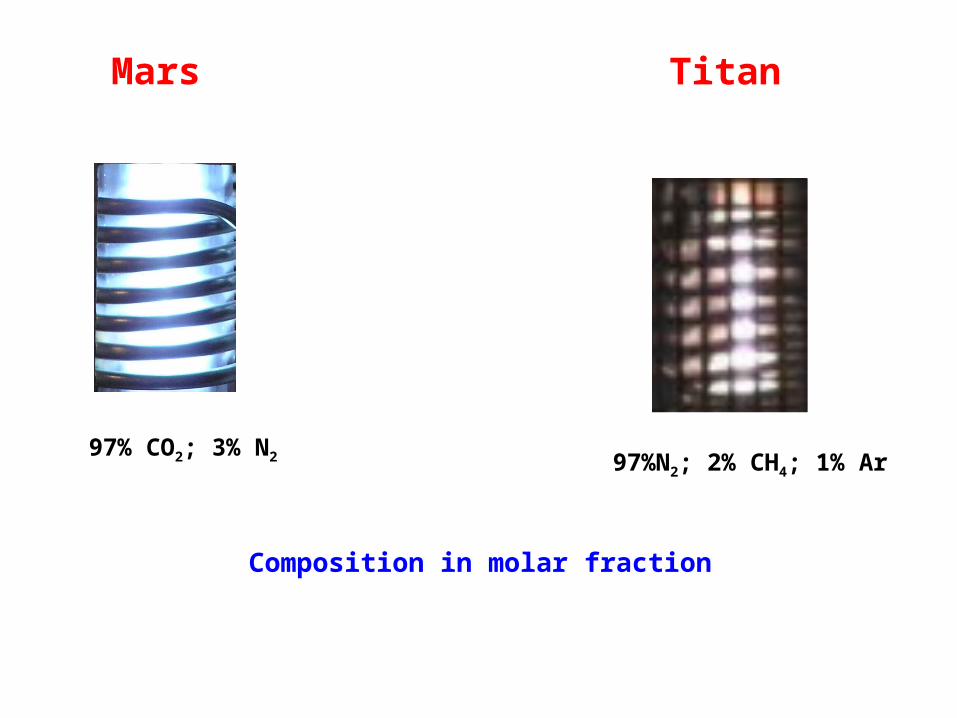
Composition in molar fraction

Mars

97% CO2; 3% N2

Titan

97%N2; 2% CH4; 1% Ar

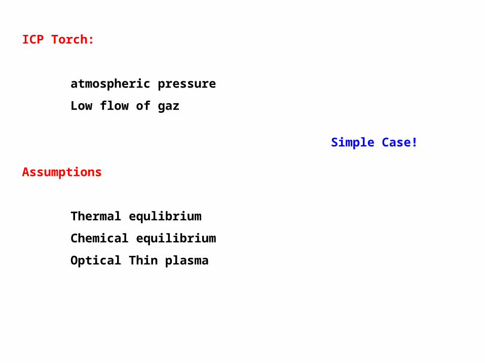
ICP Torch:

atmospheric pressure

Low flow of gaz

Assumptions

Thermal equlibrium

Chemical equilibrium

Optical Thin plasma

Simple Case!

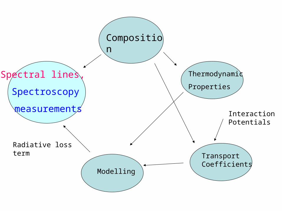
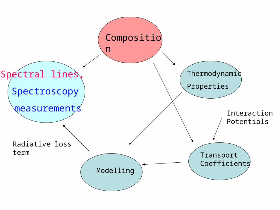
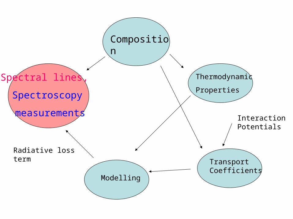
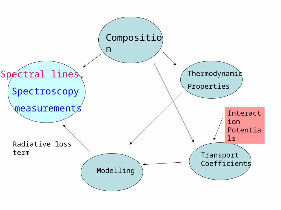
Composition

Spectral lines,

Spectroscopy

measurements

Transport Coefficients

Modelling

Thermodynamic

Properties

Radiative loss term

Interaction Potentials

Composition

Spectral lines,

Spectroscopy

measurements

Transport Coefficients

Modelling

Thermodynamic

Properties

Radiative loss term

Interaction Potentials

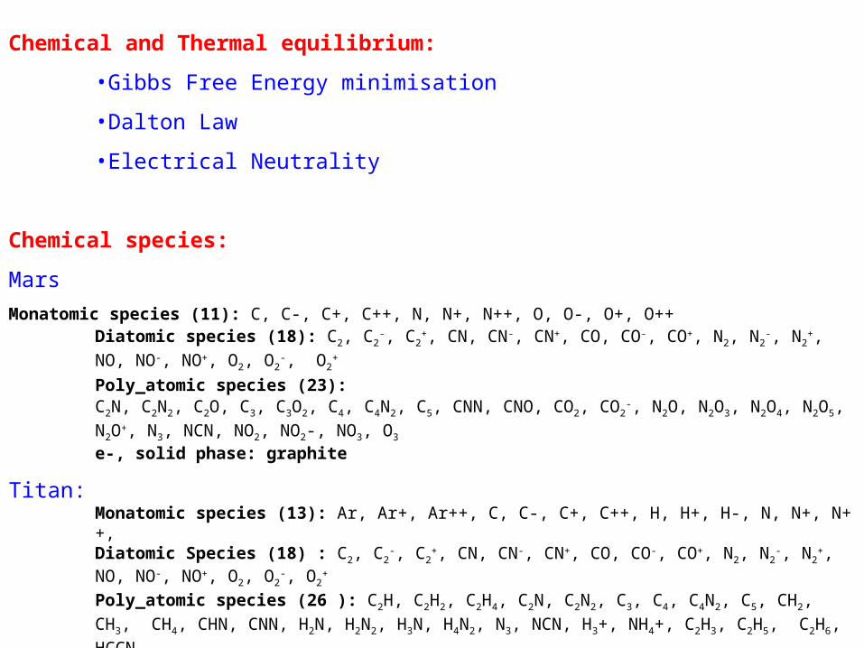
Chemical and Thermal equilibrium:

•Gibbs Free Energy minimisation

•Dalton Law

•Electrical Neutrality

Chemical species:

Mars

Monatomic species (11): C, C-, C+, C++, N, N+, N++, O, O-, O+, O++Diatomic species (18): C2, C2

-, C2+, CN, CN-, CN+, CO, CO-, CO+, N2, N2

-, N2+, NO, NO-, NO+, O2, O2

-,

O2+

Poly_atomic species (23):C2N, C2N2, C2O, C3, C3O2, C4, C4N2, C5, CNN, CNO, CO2, CO2

-, N2O, N2O3, N2O4, N2O5, N2O+, N3,

NCN, NO2, NO2-, NO3, O3 e-, solid phase: graphite

Titan:Monatomic species (13): Ar, Ar+, Ar++, C, C-, C+, C++, H, H+, H-, N, N+, N++, Diatomic Species (18) : C2, C2

-, C2+, CN, CN-, CN+, CO, CO-, CO+, N2, N2

-, N2+, NO, NO-, NO+, O2,

O2-, O2

+

Poly_atomic species (26 ): C2H, C2H2, C2H4, C2N, C2N2, C3, C4, C4N2, C5, CH2, CH3, CH4, CHN,

CNN, H2N, H2N2, H3N, H4N2, N3, NCN, H3+, NH4+, C2H3, C2H5, C2H6, HCCNe-, solid phase: graphite

10-6

10-4

10-2

100

1500 3000 4500 6000

NC

C+

e-

NCNNH

CH

C2

C2NC

2H

C2H

2

H

CHN

Ar

C(S)

H2

H

N2

Temperature (K)F

ract

ion

mo

laire

10-6

10-4

10-2

100

1500 3000 4500 6000

CN

e- NO+

C

NO2

N

NO

OO2

CON

2

CO2

Temperature (K)

Fra

ctio

n m

ola

ire

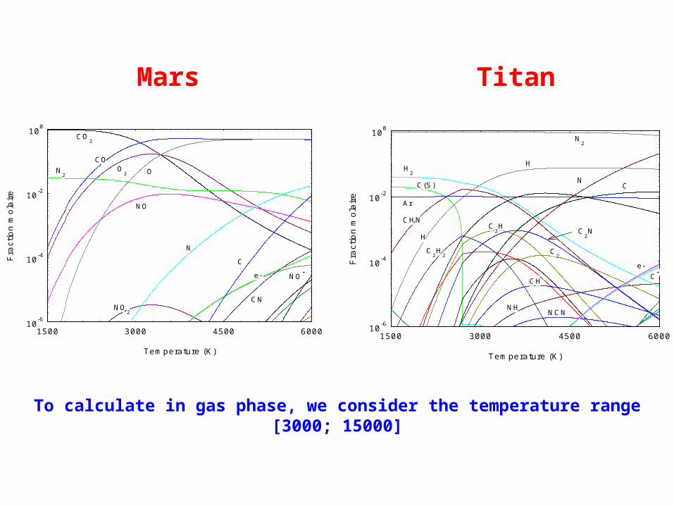
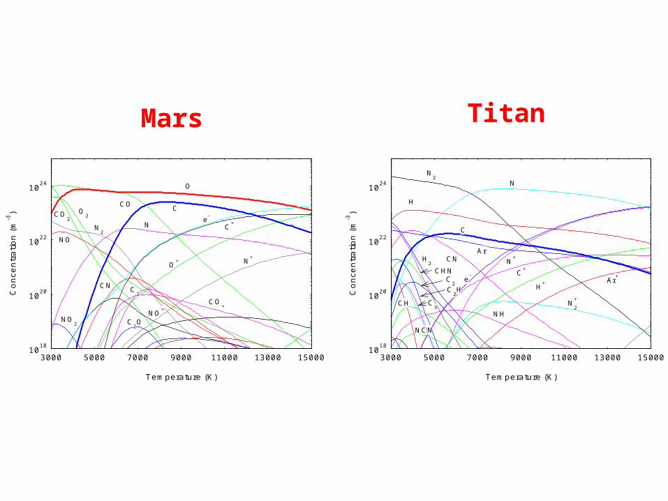
To calculate in gas phase, we consider the temperature range [3000; 15000]

Mars Titan

1018

1020

1022

1024

3000 5000 7000 9000 11000 13000 15000

C2

NO2 C

2O

NO+

CN

CO+

CO2

O2

N2

NO

N+

O+

C+e-

N

CCO

O

Temperature (K)

Con

cent

ratio

n (m

-3)

Mars Titan

1018

1020

1022

1024

3000 5000 7000 9000 11000 13000 15000

N+

NCN

CH C3

C2H

C2

CHNH

2

NHN

2

+

Ar+

H+

C+

e-

ArCN

C

H

NN

2

Temperature (K)

Con

cent

ratio

n (m

-3)

Composition

Spectral lines,

Spectroscopy

measurements

Transport Coefficients

Modelling

Thermodynamic

Properties

Radiative loss term

Interaction Potentials

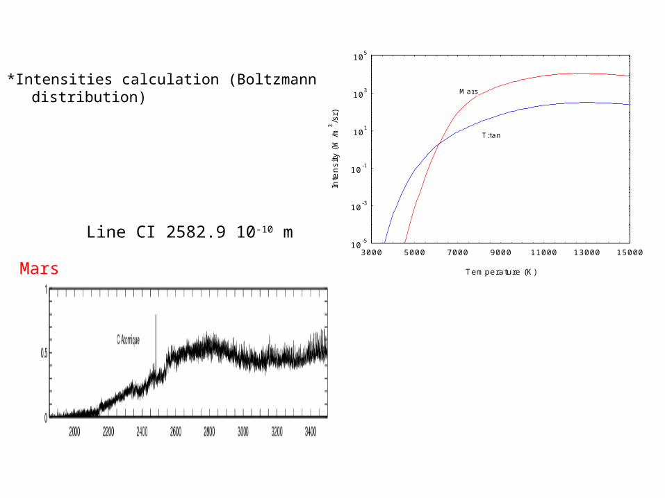
*Intensities calculation (Boltzmann distribution)

Mars

Line CI 2582.9 10-10 m10

-5

10-3

10-1

101

103

105

3000 5000 7000 9000 11000 13000 15000

Titan

Mars

Temperature (K)

Inte

nsi

ty (

W/m

3/s

r)

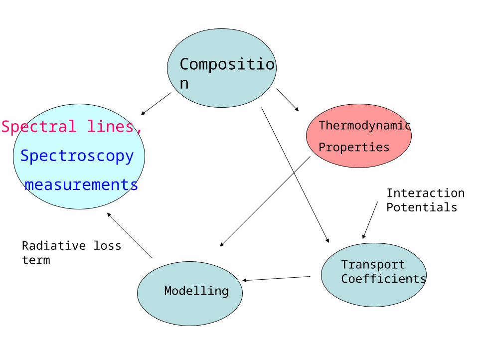
Composition

Spectral lines,

Spectroscopy

measurements

Transport Coefficients

Modelling

Thermodynamic

Properties

Radiative loss term

Interaction Potentials

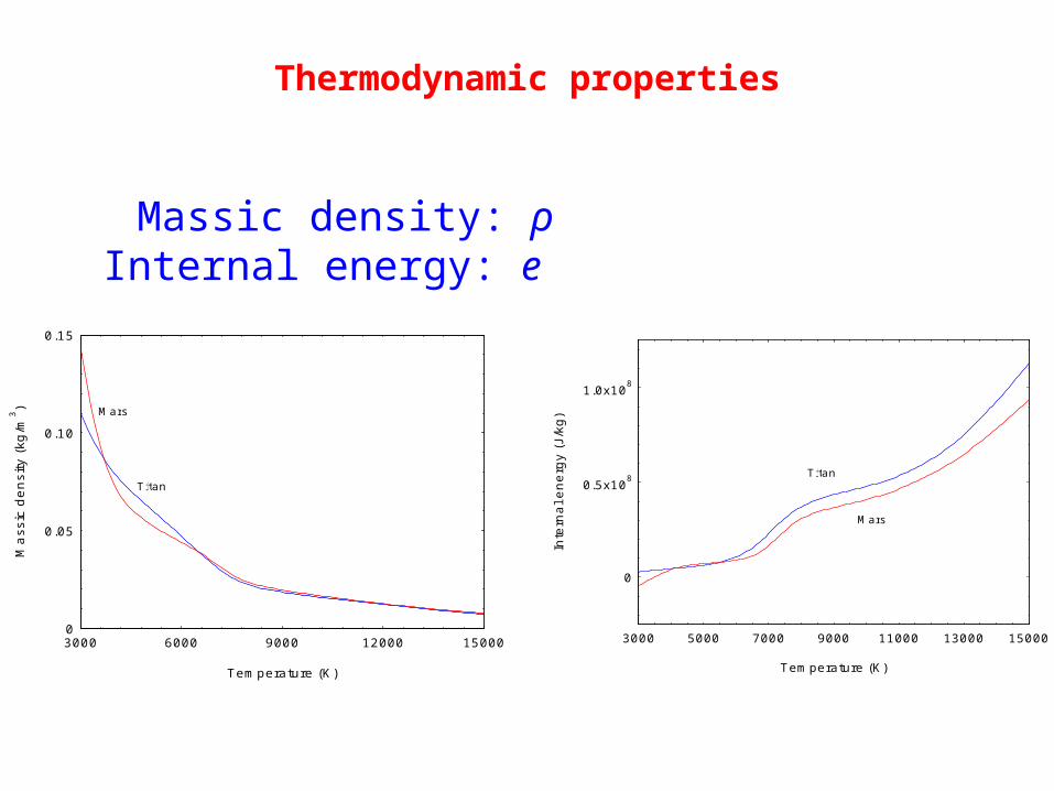
Thermodynamic properties

Massic density: ρ Internal energy: e

0

0.05

0.10

0.15

3000 6000 9000 12000 15000

Mars

Titan

Temperature (K)

Mas

sic

dens

ity (

kg/m

3)

0

0.5x108

1.0x108

3000 5000 7000 9000 11000 13000 15000

Titan

Mars

Temperature (K)

Inte

rna

l en

erg

y (J

/kg

)

Composition

Spectral lines,

Spectroscopy

measurements

Transport Coefficients

Modelling

Thermodynamic

Properties

Radiative loss term

Interaction Potentials

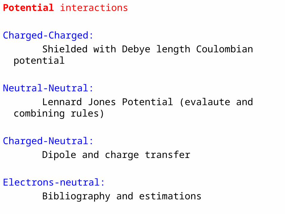
Potential interactions

Charged-Charged:

Shielded with Debye length Coulombian potential

Neutral-Neutral:

Lennard Jones Potential (evalaute and combining rules)

Charged-Neutral:

Dipole and charge transfer

Electrons-neutral:

Bibliography and estimations

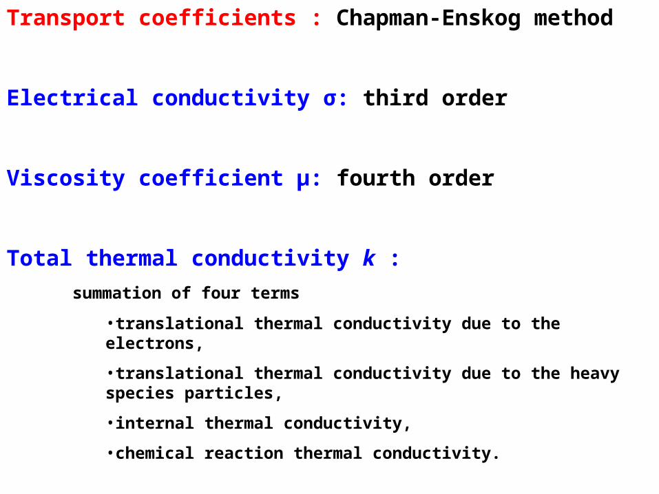
Transport coefficients : Chapman-Enskog method

Electrical conductivity σ: third order

Viscosity coefficient μ: fourth order

Total thermal conductivity k :

summation of four terms

•translational thermal conductivity due to the electrons,

•translational thermal conductivity due to the heavy species particles,

•internal thermal conductivity,

•chemical reaction thermal conductivity.

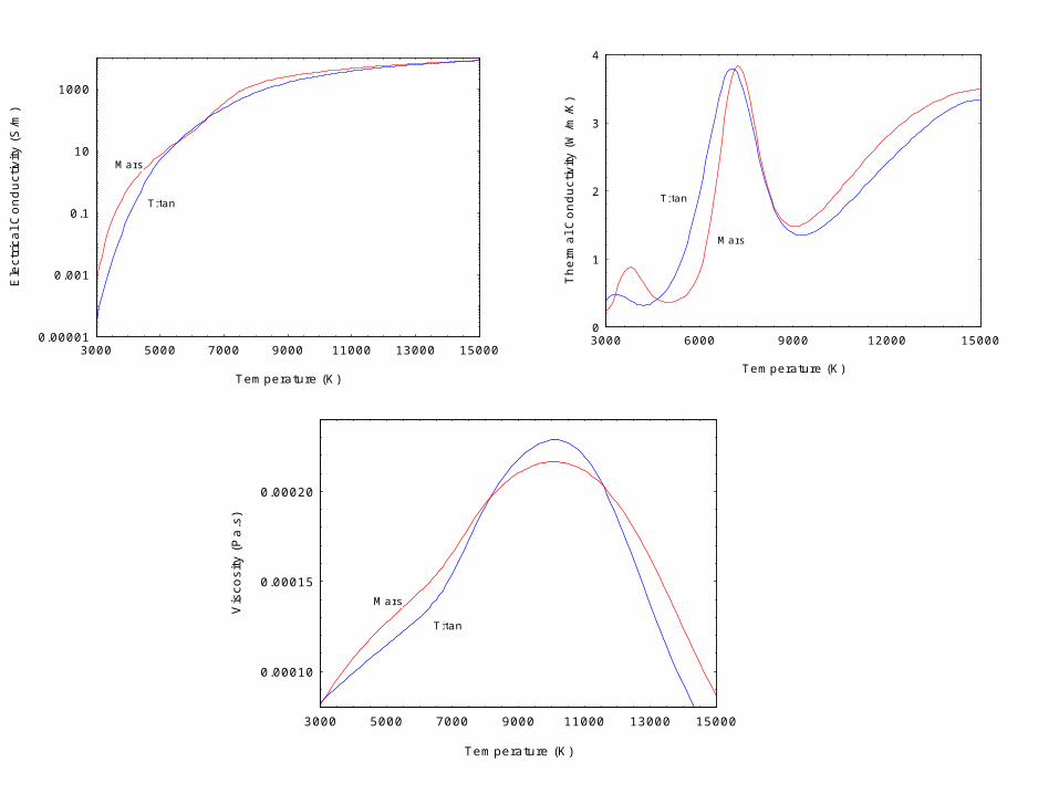
0.00001

0.001

0.1

10

1000

3000 5000 7000 9000 11000 13000 15000

Mars

Titan

Temperature (K)

Ele

ctri

cal C

on

du

ctiv

ity (

S/m

)

0.00010

0.00015

0.00020

3000 5000 7000 9000 11000 13000 15000

Titan

Mars

Temperature (K)

Vis

cosi

ty (

Pa

.s)

0

1

2

3

4

3000 6000 9000 12000 15000

Titan

Mars

Temperature (K)

Th

erm

al C

ond

uct

ivity

(W

/m/K

)

Axisymmetry LTE model for inductive plasma torches

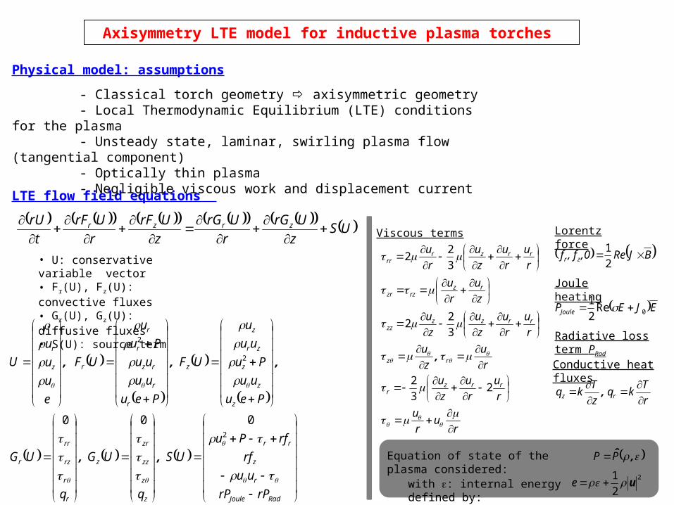
LTE flow field equations

USz

UrG

r

UrG

z

UrF

r

UrF

t

rU zrzr

RadJoule

r

z

rr

z

z

zz

zr

z

r

r

rz

rr

r

z

z

z

zr

z

z

r

r

rz

r

r

rz

r

rPrP

uu

rf

rfPu

US

q

UG

q

UG

Peu

uu

Pu

uu

u

UF

Peu

uu

uu

Pu

u

UF

e

u

u

u

U

2

2

2

000

,,

,,,

• U: conservative variable vector• Fr(U), Fz(U): convective fluxes

• Gr(U), Gz(U): diffusive fluxes• S(U): source term

ru

r

u

r

u

r

u

z

ur

u

z

u

r

u

r

u

z

u

z

u

z

u

r

u

r

u

r

u

z

u

r

u

rrzr

rz

rrzzzz

rzrzzr

rrzrrr

23

2

3

22

3

22

,

Equation of state of the plasma considered: ,P̂P

with : internal energy defined by:2

2

1u e

Viscous terms

r

Tkq

z

Tkq rz

,

Conductive heat fluxes

Lorentz force

BJRe,0f,f zr 2

1

Joule heating

EJEPJoule 0Re2

1

Radiative loss term PRad

Physical model: assumptions

- Classical torch geometry axisymmetric geometry- Local Thermodynamic Equilibrium (LTE) conditions for the plasma- Unsteady state, laminar, swirling plasma flow (tangential component)- Optically thin plasma- Negligible viscous work and displacement current

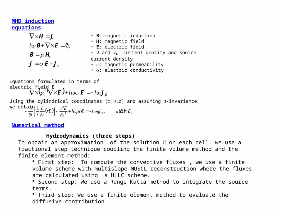
MHD induction equations

0

0

JEJ

H,B

,EB

J,H

i

01 JEE ii

• B: magnetic induction• H: magnetic field• E: electric field• J and J0: current density and source current density• : magnetic permeability• : electric conductivity

Equations formulated in terms of electric field E

Numerical method

Hydrodynamics (three steps)To obtain an approximation of the solution U on each cell, we use a fractional step technique coupling the finite volume method and the finite element method:

First step: To compute the convective fluxes , we use a finite volume scheme with multislope MUSCL reconstruction where the fluxes are calculated using a HLLC scheme. Second step: We use a Runge Kutta method to integrate the source terms. Third step: We use a finite element method to evaluate the diffusive contribution.

ElectromagneticTo solve the partial differential equation, we use a standard finite element method with a standard triangulation of the domain and the use of a piecewise linear approximation.

Using the cylindrical coordinates (r,,z) and assuming -invariance we obtain:

EEJiEiz

ErE

rrr

with 1

02

2

,

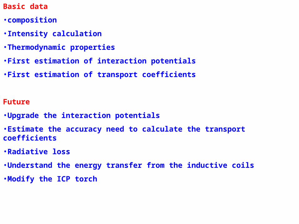
Basic data

•composition

•Intensity calculation

•Thermodynamic properties

•First estimation of interaction potentials

•First estimation of transport coefficients

Future

•Upgrade the interaction potentials

•Estimate the accuracy need to calculate the transport coefficients

•Radiative loss

•Understand the energy transfer from the inductive coils

•Modify the ICP torch