models for innovative factory layout design techniques and

FACULDADE DE ENGENHARIA DA UNIVERSIDADE DO PORTO

Models for innovative factory layoutdesign techniques and adaptive

reconfiguration in the automotiveindustry

José Manuel da Rocha Pimenta Soares

FOR JURY EVALUATION

Mestrado Integrado em Engenharia Eletrotécnica e de Computadores

Supervisor: Gil Gonçalves

January 25, 2016

c© José Soares, 2015

Resumo

À medida que a pressão competitiva de países emergentes aumenta e se faz sentir na europa,os líderes da indústria europeia são forçados a tomar a difícil decisão de cortar não apenas noscustos não apenas dos produtos, mas também nos investimentos em equipamento, planeamentodas fábricas, operação et... tudo isto sem comprometer a qualidade que a caracteriza.

O projecto ReBORN, procura desenvolver uma série de estratégias e tecnologias que suportamum novo paradigma para a reutilização de equipamentos de produção industriais no momento daconcepção e planeamento de novas linhas de produção. Estas estratégias abordam questões rele-vantes na indústria actual, como a falta de uma metodoliogia mais abrangente que inclua métodospara aferir o custo total de vida, o impacto ambiental e a fiabilidade das máquinas a serem instal-adas, no processo de planeamento das novas linha de produção.

No contexto do projecto uma ferramenta de simulação (High Performance Simulation tool)está a ser criada pelos vária parceiros envolvidos, que ajudará na decisão da escolha das melhoresmáquinas a integrar uma dada linha de produção. Esta ferramenta cria vários layouts possíveisque serão depois simulados com o intuito de aferir o seu Life-cycle Cost (custo de vida), Life-cycleAssessment (análise ao impacto ambiental) e a sua fiabilidade.

O trabalho desenvolvido nesta dissertação centrou-se em desenvolver uma ferramenta que fa-cilite a criação de modelos de simulação das linhas de produção, de forma a aferir a sua fiabilidade.

Desta forma, foi desenvolvido um interface que controla remotamente o Flexsim - softwarede simulação usado. Este interface gera automaticamente o modelo das linhas de produção noFlexsim, com base na sua descrição num ficheiro XML.

Do lado do Flexsim, foi criado um novo objecto de simulação que representa as máquinas,cujas funcionalidades adicionais permitem complementar os modelos gerados pelo interface.

i

Abstract

With the competitive pressure form emerging countries increasing, European manufacturing in-dustry leaders have to rethink the costs of not only products, but also investments in equipment,factory planing, ramp-up and operation. All of this without compromising the quality of its prod-ucts.

The ReBORN project seeks to demonstrate technologies and strategies that support the a newparadigm for re-use of production equipment when designing installing new production lines.These strategies and technologies will address relevant issues in today’s manufacturing, such asthe lack of comprehensive design methodology for manufacturing systems or the nonexistence ofappropriate methods for dynamic cost assessment for system design and system life-cycle opti-mization.

A High Performance Simulation tool is being developed by the several partners that will assistthe new production line planner in making the best choices regarding machines and other pro-duction equipment. This tool creates several possible layouts for a job description based on thecapabilities of the machines and equipment available, that is then simulated in order to assess theproduction machines regarding their Life-cycle Cost, Life-cycle Assessment and their Reliability.

The work developed in this dissertation focused on developing a tool that facilitates the cre-ation of simulation models of the production lines in order to assess their reliability.

An Interface was developed that controls Flexsim - the simulation software used- remotely.This Interface generates the production lines’ simulation models automatically from their descrip-tian in XML files. On Flexsim’s side a new class of Processor was created, that has added featuresto complete the simulation model generated by the Interface.

iii

Contents

1 Introduction 11.1 Motivation . . . . . . . . . . . . . . . . . . . . . . . . . . . . . . . . . . . . . . 11.2 Scope . . . . . . . . . . . . . . . . . . . . . . . . . . . . . . . . . . . . . . . . 11.3 Goals . . . . . . . . . . . . . . . . . . . . . . . . . . . . . . . . . . . . . . . . 11.4 Document Overview . . . . . . . . . . . . . . . . . . . . . . . . . . . . . . . . 2

2 Literature Review 32.1 Manufacturing Systems . . . . . . . . . . . . . . . . . . . . . . . . . . . . . . . 3

2.1.1 Flexible Manufacturing Systems . . . . . . . . . . . . . . . . . . . . . . 32.1.2 Reconfigurable Manufacturing Systems . . . . . . . . . . . . . . . . . . 42.1.3 Intelligent Manufacturing Systems . . . . . . . . . . . . . . . . . . . . 5

2.2 Lifecycle Costing . . . . . . . . . . . . . . . . . . . . . . . . . . . . . . . . . . 72.3 Life Cycle Assessment . . . . . . . . . . . . . . . . . . . . . . . . . . . . . . . 82.4 Reliability Assessment . . . . . . . . . . . . . . . . . . . . . . . . . . . . . . . 102.5 Reliability Modeling . . . . . . . . . . . . . . . . . . . . . . . . . . . . . . . . 11

2.5.1 Basic models for Parts (Life Distribution Models) . . . . . . . . . . . . . 122.5.2 Physical Acceleration . . . . . . . . . . . . . . . . . . . . . . . . . . . . 142.5.3 Bottom-up approach to System Reliability . . . . . . . . . . . . . . . . . 162.5.4 Basic Models for Repairable systems . . . . . . . . . . . . . . . . . . . 19

2.6 Overall Equipment Effectiveness . . . . . . . . . . . . . . . . . . . . . . . . . . 192.7 Manufacturon . . . . . . . . . . . . . . . . . . . . . . . . . . . . . . . . . . . . 202.8 Simulation . . . . . . . . . . . . . . . . . . . . . . . . . . . . . . . . . . . . . . 20

2.8.1 Limitation to current simulation techniques . . . . . . . . . . . . . . . . 222.8.2 Simulation Package . . . . . . . . . . . . . . . . . . . . . . . . . . . . . 22

2.9 Data Format for Information Exchange . . . . . . . . . . . . . . . . . . . . . . . 222.9.1 AutomationML . . . . . . . . . . . . . . . . . . . . . . . . . . . . . . . 232.9.2 Core Manufacturing Simulation Data . . . . . . . . . . . . . . . . . . . 23

3 Problem Analysis 253.1 VERSONs . . . . . . . . . . . . . . . . . . . . . . . . . . . . . . . . . . . . . . 253.2 Overview of the High Performance Simulation Tool . . . . . . . . . . . . . . . . 263.3 Problem specification . . . . . . . . . . . . . . . . . . . . . . . . . . . . . . . . 28

4 Machine Concept for the simulation models 314.1 Machine as a system . . . . . . . . . . . . . . . . . . . . . . . . . . . . . . . . 31

4.1.1 Socket Level . . . . . . . . . . . . . . . . . . . . . . . . . . . . . . . . 324.2 Lifetime modeling . . . . . . . . . . . . . . . . . . . . . . . . . . . . . . . . . 32

4.2.1 Lifetime distributions . . . . . . . . . . . . . . . . . . . . . . . . . . . . 32

v

vi CONTENTS

4.2.2 Accelerated Lifetime models . . . . . . . . . . . . . . . . . . . . . . . . 324.2.3 Lifetime information . . . . . . . . . . . . . . . . . . . . . . . . . . . . 34

5 Implementation 355.1 Overview of Process . . . . . . . . . . . . . . . . . . . . . . . . . . . . . . . . 355.2 Data Structure . . . . . . . . . . . . . . . . . . . . . . . . . . . . . . . . . . . . 365.3 Flexsim Remote Control . . . . . . . . . . . . . . . . . . . . . . . . . . . . . . 38

5.3.1 Explored alternatives . . . . . . . . . . . . . . . . . . . . . . . . . . . . 385.3.2 Solution adopted . . . . . . . . . . . . . . . . . . . . . . . . . . . . . . 39

5.4 Interface . . . . . . . . . . . . . . . . . . . . . . . . . . . . . . . . . . . . . . . 395.4.1 Overview of the Interface . . . . . . . . . . . . . . . . . . . . . . . . . 405.4.2 Automatic model generation from XML . . . . . . . . . . . . . . . . . . 41

5.5 Flexsim Models . . . . . . . . . . . . . . . . . . . . . . . . . . . . . . . . . . . 425.5.1 Basic Flexsim concepts . . . . . . . . . . . . . . . . . . . . . . . . . . . 425.5.2 Implemented Models . . . . . . . . . . . . . . . . . . . . . . . . . . . . 435.5.3 Shortcomings in the implementation . . . . . . . . . . . . . . . . . . . . 445.5.4 Outcome of the Simulations . . . . . . . . . . . . . . . . . . . . . . . . 45

6 Conclusions and Future Work 476.1 Conclusions . . . . . . . . . . . . . . . . . . . . . . . . . . . . . . . . . . . . . 476.2 Future Work . . . . . . . . . . . . . . . . . . . . . . . . . . . . . . . . . . . . . 48

A Common formulas and plots for lifetime models 49A.1 Exponential . . . . . . . . . . . . . . . . . . . . . . . . . . . . . . . . . . . . . 49A.2 Weibull . . . . . . . . . . . . . . . . . . . . . . . . . . . . . . . . . . . . . . . 51A.3 Lognormal . . . . . . . . . . . . . . . . . . . . . . . . . . . . . . . . . . . . . . 53

B Schematics for bottom-up Reliability 57B.1 Series Model . . . . . . . . . . . . . . . . . . . . . . . . . . . . . . . . . . . . 57B.2 Parallel Model . . . . . . . . . . . . . . . . . . . . . . . . . . . . . . . . . . . . 58B.3 Complex Model . . . . . . . . . . . . . . . . . . . . . . . . . . . . . . . . . . . 59

List of Figures

2.1 Manufacturing system model . . . . . . . . . . . . . . . . . . . . . . . . . . . . 42.2 Life Cycle stages . . . . . . . . . . . . . . . . . . . . . . . . . . . . . . . . . . 92.3 Phases of an LCA . . . . . . . . . . . . . . . . . . . . . . . . . . . . . . . . . . 92.4 Example of a system reliability model [1] . . . . . . . . . . . . . . . . . . . . . 112.5 Bathtub Curve for parts [2] . . . . . . . . . . . . . . . . . . . . . . . . . . . . 142.6 Example of a production line model in Flexsim . . . . . . . . . . . . . . . . . . 23

3.1 ReBORN high performance simulation tool [3] . . . . . . . . . . . . . . . . . . 273.2 Example of a comparison of an LCC assessment in two machines . . . . . . . . 29

4.1 Illustration of Renewal Process [4] . . . . . . . . . . . . . . . . . . . . . . . . . 324.2 Example of evolution of step-load levels over operating time . . . . . . . . . . . 334.3 Equivalent failure probability with 3 different load conditions . . . . . . . . . . . 34

5.1 Overview of the solution’s methodology . . . . . . . . . . . . . . . . . . . . . . 355.2 Example of a layout defined in XML . . . . . . . . . . . . . . . . . . . . . . . . 375.3 Example of a layout defined in XML . . . . . . . . . . . . . . . . . . . . . . . . 41

A.1 Exponential PDF plots [2] . . . . . . . . . . . . . . . . . . . . . . . . . . . . . 50A.2 Exponential CDF plots [2] . . . . . . . . . . . . . . . . . . . . . . . . . . . . . 50A.3 Examples of Weibull PDF plots [2] . . . . . . . . . . . . . . . . . . . . . . . . 52A.4 Weibull Failure Rate plots for different values of β [2] . . . . . . . . . . . . . . 52A.5 Examples of Lognormal PDF plots [2] . . . . . . . . . . . . . . . . . . . . . . 54A.6 Examples of Lognormal Failure rate plots [2] . . . . . . . . . . . . . . . . . . . 55

B.1 Example of a Series model [2] . . . . . . . . . . . . . . . . . . . . . . . . . . . 57B.2 Example of a Series model [2] . . . . . . . . . . . . . . . . . . . . . . . . . . . 58B.3 Example of a Complex model [2] . . . . . . . . . . . . . . . . . . . . . . . . . 59

vii

viii LIST OF FIGURES

Abbreviations

ABS Agent Based SimulationCDF Cumulative Distribution FunctionCIM Computer Integrated ManufacturingCIM Computer Integrated ManufacturingCMSD Core Manufacturing Simulation DataCNC Computer Numerical ControlCOM Component Object ModelCOM Component Object ModelDES Discrete Event SimulationDES Discrete Event SimulationDLL Dinamic-Link LibraryDLL Dynamic-link libraryDMS Distributed Manufacturing SystemDOM Document Object ModelERP Enterprise Resource PlanningFMS Flexible Manufacturing SystemFOM Force of MortalityGUI Graphical User interfaceHTML Hypertext Markup LanguageIDE Integrated Development EnvironmentIID Independent and Identically DistributedIMS Computer Aided DesignIMS Intelligent Manufacturing SystemLCA Life Cycle AssessmentLCC Life Cycle CostingMAS Muli-Agent SystemMAS Multi-agent SystemsMRP2 Manufacturing Resource PlanningMTBF Mean Time Before FailureMTTF Mean Time to FailureMTTR Mean Time To RepairOEE Overall Equipment EfficiencyCIM Computer Integrated ManufacturingPDF Probability Density FunctionRMS Reconfigurable Manufacturing SystemSD Computer Aided DesignVERSON Versatile, Flexible Lifecycle Extended DevicesXML eXtensible Markup Language

ix

Chapter 1

Introduction

1.1 Motivation

Industrial manufacturing is characterized by fierce competition on a global scale. The pressure to

cut costs from emerging countries, forces the European industry to think over the costs of both

the products, as well as their investments in equipment, factory planing, ramp-up and operation

without compromising the quality of its products.

The ReBORN project, is an European consortium that incorporates academic and research

institutions as well as companies in the industrial manufacturing sector. It envisions the demon-

stration of strategies and technologies that support the a new paradigm for re-use of production

equipment in old, renewed and new factories, maximizing the efficiency of this re-use and mak-

ing the factory design process much easier and straight forward, shortening ramp-up times and

increasing production efficiency and flexibility. This paradigm will give new life to decommis-

sioned production systems and equipment, making it possible their “reborn” in new production

lines

1.2 Scope

A High Performance Simulation tool is being developed by several partners in ReBORN which

will take advantage of system information for real time system adaptation and use it in improving

overall system performance throughout its life-cycle.

The purpose is to tackle relevant issues in today’s manufacturing, such as the lack of com-

prehensive design methodology for manufacturing systems or the nonexistence of appropriate

methods for dynamic cost assessment for system design and system life-cycle optimization.

1.3 Goals

The purpose of the work developed for the thesis is to provide a tool that facilitates the creation of

simulation models of production lines, in order to produce a various metrics that will be used in

1

2 Introduction

three assessments: (1) Reliability assessment, (2) Life Cycle Cost and (3) Life Cycle Assessment.

1.4 Document Overview

In Chapter 2 important concepts for both ReBORN and the tool to be developed are presented. The

context of the research is analyzed and related work is reviewed. Chapter 3 presents an overview of

the project, and proceeds to detail the subsystem to be addressed. In Chapter 5 the implementation

is described, specifying the several components that were developed, their integration and the

models proposed. In Chapter 6 Conclusions are drawn and Future work is suggested.

Chapter 2

Literature Review

In this chapter, an introduction is made to the concepts of LCC, LCA and Reliability, which are

in the core of the process studied in this thesis. In the next section a brief account of the evolution

of manufacturing systems in the 20th century is made and finally other concepts that support

ReBORn like Intelligent Agents, Simulation and previous related projects are also introduced.

2.1 Manufacturing Systems

Like other business sectors, industry is driven by profit, reputation and market share. From the

turn of the 20th century, with the invention of the moving assembly line by Henry Ford and the

introduction of Mass Production as a paradigm until the present day, enterprises must implement

manufacturing systems that are able to meet market demands and effectively and efficiently ad-

dress the requirements of the environment in which they operate. Currently, these requirements

are understood to be the following [5] :

• Short lead time;

• More variants;

• Low and fluctuating volumes;

• Low price.

Figure 2.1 shows a model of a manufacturing system.

In the following sections a brief description of different paradigms in industry are described,

with special relevance for Intelligent Manufacturing Systems, and its related concepts.

2.1.1 Flexible Manufacturing Systems

In the 1980’s Flexible Manufacturing Systems (FMS) were introduced. FMS is a programmable

machining system configuration which incorporates software to handle changes in work orders,

3

4 Literature Review

Figure 2.1: Manufacturing system model

production schedules, part-programs, and tooling for production of a family of parts. The objec-

tive of a FMS is to make possible the manufacture of several families of parts, with shortened

changeover time, on the same system. [6]

2.1.2 Reconfigurable Manufacturing Systems

In the mid 1990’s, a new concept was introduced, the Reconfigurable Manufacturing System(RMS).

It is basically a machining system which can be created by incorporating basic process modules-

both hardware and software that can be rearranged or replaced quickly and reliably. [6] Recon-

figuration allows adding, removing, or modifying specific process capabilities, controls, software

or machine structure to adjust production capacity in response to changing market demands or

technologies. [6] RMS provides customized flexibility for a particular part-family and will be

open-ended, so that it can be improved, upgraded and reconfigured, rather than replaced. RMS are

marked by six core reconfigurable characteristics [7]:

• Customization

• Convertibility

• Scalability

• Modularity

• Integrality

• Diagnosability

2.1 Manufacturing Systems 5

The components of RMS are CNC machines, Reconfigurable Machine Tools, Reconfigurable

Inspection Machines and material transport systems (such as gantries and conveyors) that connect

the machines to form the system. Different arrangements and configurations of these machines

will have an impact on the system productivity [5].

The purpose of an RMS is to provide exactly when it is needed. RMS goes beyond the objec-

tives of FMS by permitting [6]:

• Reduction of lead time for launching new systems and reconfiguring existing systems

• The rapid modification and quick integration of new technology and/or new functions into

existing systems

2.1.3 Intelligent Manufacturing Systems

In order to meet the new requirements listed in 2.1, the concept of Computer Integrated Man-ufacturing (CIM) was created. It is characterized by the centralized control of a completely

automated factory, where decision-making is broadcast from higher hierarchical levels down to

operational units. It integrates operational functions and business level tools, like Manufactur-

ing Resource Planning (MRP2) and Enterprise Resource Planning (ERP). On the downside, the

complexity of its structures and the high investments necessary can lead to rigid systems [8].

In order for companies to survive fierce market competition and volatility, as well as the demand

for more flexibility and reactivity, they had to become more agile. Agility can be seen as "the

ability to operate with a high level of coordination and pro-activity throughout the supply chain,

simultaneously reacting to disturbances on the shop floor efficiently while taking the increasing

process complexity (e.g., variabilities, high product variety, reconfiguration issues) into account"

[9].

Because of CIM rigid nature and therefore inability to be agile, researchers turned to dis-tributed architectures, Distributed Manufacturing Systems (DMS), where autonomous entities

have the capacity to make decisions without a centralized view. These systems are called Intelli-

gent Manufacturing Systems (IMS) and they are characterized by: [10]:

• autonomy,

• decentralization,

• reliability

• flexibility

• efficiency

• learning

• self-regeneration

6 Literature Review

Several approaches to IMS have been proposed like Fractal Manufacturing Systems, Bionic

Manufacturing Systems, Holonic Manufacturing Systems, Product Driven Manufacturing Sys-

tems and Agent-Based Manufacturing [8] [9], combining elements of a centralized control e.g.

its predictability, with the agility and robustness of DMS [9]. The common ground to these ap-

proaches are the concepts of Agent 2.1.3.1 and Multi-Agent System 2.1.3.2.

In general, IMS need to meet certain requirements such as: [11]

• Full integration of heterogeneous software and hardware systems within an enterprise, a

virtual enterprise, or across a supply chain;

• Open system architecture to accommodate new subsystems (software or hardware) or dis-

mantle existing subsystems “on the fly”;

• Efficient and effective communication and cooperation among departments within an enter-

prise and among enterprises;

• Embodiment of human factors into manufacturing systems;

• Quick response to external order changes and unexpected disturbances from both internal

and external manufacturing environments;

• Fault tolerance both at the system level and at the subsystem level so as to detect and recover

from system failures and minimize their impacts on the workflow environment.

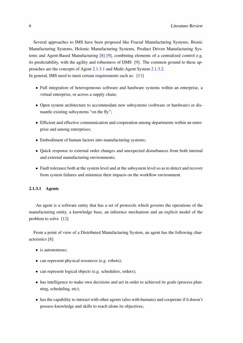
2.1.3.1 Agents

An agent is a software entity that has a set of protocols which governs the operations of the

manufacturing entity, a knowledge base, an inference mechanism and an explicit model of the

problem to solve [12]

From a point of view of a Distributed Manufacturing System, an agent has the following char-

acteristics [8]:

• is autonomous;

• can represent physical resources (e.g. robots);

• can represent logical objects (e.g. schedulers, orders);

• has intelligence to make own decisions and act in order to achieved its goals (process plan-

ning, scheduling, etc);

• has the capability to interact with other agents (also with humans) and cooperate if it doesn’t

possess knowledge and skills to reach alone its objectives;

2.2 Lifecycle Costing 7

• can interact in the environment where is inserted (e.g. production environment) feeling and

changing it based on the knowledge that it contains;

• reacts to context incentives and defines actuation plans based in his knowledge;

• can decide if it accepts or rejects a service requested by other agent, based in its knowledge

and skills;

• has capacity to acquire and to memorize new knowledge.

2.1.3.2 Multi-Agent Systems

A Multi-Agent System (MAS) is a system composed of different agents that interact with

each other in planning and executing their responsibilities. In manufacturing, MAS view the sup-

ply chain as composed of a set of intelligent (software) agents. Each agent is autonomous, goal-

oriented software process that operates asynchronously, communicating and coordinating with

other agents as needed [10]. Almeida et. al. identified the major barriers to the adoption of MAS

by the manufacturing industry as being the deficient security of agent execution and communica-

tion, the complexity of the system, the low level of scalability, the need of standardization and the

need of a better integrated human-machine interaction.

2.2 Lifecycle Costing

Life Cycle Costing (LCC) is a process to determine the sum of all the costs associated with an

asset or with part of an asset. These costs include acquisition, installation, operation, maintenance,

refurbishment, and disposal. LCC can be carried out during any or all phases of an asset’s life

cycle. LCC process usually includes steps such as [13]:

1. Life Cost Planning: concerns the assessment and comparison of options/alternatives during

the design/ acquisition phase;

2. Selection and development of LCC model (e.g. designing cost breakdown structure, identi-

fying data sources and uncertainties;

3. Application of LCC model;

4. Documentation and review of LCC results;

5. Prepare Life Cost Analysis;

6. Implement and Monitor Life Cost Analysis.

8 Literature Review

The ultimate goal for carrying out LCC calculations is to aid decision making in:

• Assessing and controlling costs and identifying cost significant items.

• Producing selection of work and expenditure planning profiles.

LCC allows for economic justification for the sustainability considerations, as implementing

LCC in planning for construction projects shows that, over a project’s life, incorporation of sus-

tainable elements proves cost-effective as well as environmentally beneficial.

Early identification of acquisition and ownership costs enables the decision-maker to balance

performance, reliability, maintainability, maintenance support and other goals against life cycle

costs. Decisions made early in a asset’s life cycle have a much greater influence on Life Cycle

Costing than those made late in a asset’s life cycle, leading to the development of the concept of

discounted costs.

2.3 Life Cycle Assessment

Life Cycle Assessment (LCA) is a methodological framework for estimating and assessing the

environmental impacts attributable to the life cycle of a product, such as climate change, strato-

spheric ozone depletion, tropospheric ozone (smog) creation, eutrophication, acidification, toxi-

cological stress on human health and ecosystems, the depletion of resources, water use, land use,

and noise—and others. [14]

Life cycle assessment is a “cradle-to-grave” approach for assessing industrial systems. “Cradle-

to-grave” begins with the gathering of raw materials from the earth to create the system and ends

at the point when all materials are returned to the earth. LCA evaluates all stages of a product’s

life from the perspective that they are interdependent, meaning that one operation leads to the next.

LCA enables the estimation of the cumulative environmental impacts resulting from all stages in

the product life cycle, often including impacts not considered in more traditional analyses (e.g.,

raw material extraction, material transportation, ultimate product disposal, etc.). By including the

impacts throughout the product life cycle, LCA provides a comprehensive view of the environ-

mental aspects of the product or process and a more accurate picture of the true environmental

trade-offs in product and process selection.

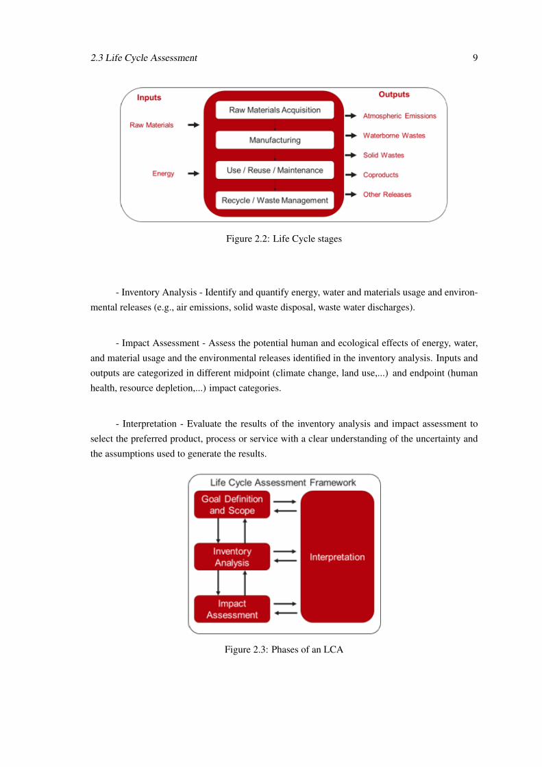
The LCA process is a systematic, phased approach and consists of four components as illus-

trated in Figure 2.2, page 9:

- Goal Definition and Scope - Define and describe the product, process or activity. Establish

the context in which the assessment is to be made and identify the boundaries and environmental

effects to be reviewed for the assessment.

2.3 Life Cycle Assessment 9

Figure 2.2: Life Cycle stages

- Inventory Analysis - Identify and quantify energy, water and materials usage and environ-

mental releases (e.g., air emissions, solid waste disposal, waste water discharges).

- Impact Assessment - Assess the potential human and ecological effects of energy, water,

and material usage and the environmental releases identified in the inventory analysis. Inputs and

outputs are categorized in different midpoint (climate change, land use,...) and endpoint (human

health, resource depletion,...) impact categories.

- Interpretation - Evaluate the results of the inventory analysis and impact assessment to

select the preferred product, process or service with a clear understanding of the uncertainty and

the assumptions used to generate the results.

Figure 2.3: Phases of an LCA

10 Literature Review

2.4 Reliability Assessment

Two of the most important factors that demonstrate the capability of any manufacturing system

to deliver its uninterrupted and on-time service are the Reliability and Maintainability of its

machinery and equipment. [15] But before proceeding the study of those two concepts, one should

understand what failure is. Failure can be essentially be defined in two ways [16]:

• The termination of the ability of the product as a whole to perform its required function.

• The termination of the ability of any individual component to perform its required function.

but not the termination of the ability of the product as a whole to perform.

Reliability measures the frequency of failures, interruptions, or needed adjustments and correc-

tions, whereas the availability measures the duration of those events.

The less often a piece of equipment fails, and the less time it requires to be brought back to an

operable state should it fail, the more reliable and maintainable it is in comparison with a machine

that fails more frequently and that takes a longer period of time to repair.

Reliability and maintainability of any machinery or equipment are functions of the reliabil-

ity and maintainability of its components, subsystems, and systems. Improved reliability and

maintainability leads to lower total life-cycle costs that are necessary to maintain the competitive

edge. [15]

Equipment reliability can be quantified by a measure of Mean Time Between Failures (MTBF)

(eq.2.1), which is the average time between failure occurrences. Equipment maintainability can

be quantified by Mean Time To Repair (MTTR), which is the average time it takes to fix a failure.

Together, MTBF and MTTR make up the equipment’s availability (A), which is the percentage

of time the equipment is available for production. Availability is one of the parameters used to

calculate OEE 2.6.

MT BF =total uptime

no. o f breakdowns(2.1)

MT T R =total downtime

no. o f breakdowns(2.2)

Reliability : R = e−(time

MT BF ) (2.3)

Availability : A =MT BF

(MT BF +MT T R)(2.4)

2.5 Reliability Modeling 11

More formally, reliability is the probability that machinery /equipment can perform contin-

uously without failure, for a specified interval of time when operating under stated conditions.

Increased reliability implies less failure and consequently less downtime and loss of production.

Maintainability is a characteristic of design, installation, and operation, usually expressed as the

probability that a machine can be restored to specified operable condition (returned to a service-

able state) within a specified interval of time when maintenance action is performed in accordance

with prescribed procedures and resources. [15]

2.5 Reliability Modeling

When modeling the Reliability and Lifetime of products, it is important to understand the

object under study and distinguish between parts, components, systems and subsystems. The

analyst must choose a point at which no more detailed information about the object of analysis is

known or needs to be considered. At that point, the analyst treats the object of analysis as a "black

box". The selection of this level (e.g., component, subassembly, assembly or system) determines

the detail of the subsequent analysis.

In system reliability analysis, one constructs a "System" model from these component models.

In other words in system reliability analysis focuses on the construction of a model that represents

the times-to-failure of the entire system based on the life distributions of the components, sub-

assemblies and/or assemblies ("black boxes") from which it is composed [1], as illustrated in the

figure 2.4.

Figure 2.4: Example of a system reliability model [1]

In other words, a system is a collection of parts, components, subsystems and/or assemblies

arranged to a specific design in order to achieve desired functions with acceptable performance

and reliability.

Asher and Feingold in [17] define the basic terminology used in systems reliability as follows:


1. Part - An item which is not subject to disassembly and hence, is discarded the first time it

fails.

2. Socket - A circuit or equipment position which, at any given time, holds a part or component

of a given type.

3. System - A collection of two or more sockets and their associated parts, interconnected to

perform one or more functions.

4. Nonrepairable system - A system that is discarded the first time that it ceases to perform

satisfactorily.

5. Repairable system - A system which, after failing to perform at least one of its required

functions, can be restored to performing all of its functions by any method, other than re-

placement of the entire system.

2.5.1 Basic models for Parts (Life Distribution Models)

Life Distribution Models describe how populations of non-repairable units (i.e. Parts) fail over

time. If T is defined as the random variable "time to failure of a part", then a lifetime distribution

model can be any probability density function (PDF) f (t) defined over the range of time from

t = 0, . . . ,∞. The corresponding cumulative distribution function (CDF) F(t) gives the probability

that a randomly selected unit will fail by time t. F(t) is also called Failure probability, function

and is given by:

F(t) =∫ t

−∞

f (s)ds (2.5)

The Reliability (or Survival) function is the probability a part survives beyond time t and can

be defined by

R(t) = 1−F(t) = P(T > t)∫

∞

tf (s)ds (2.6)

If f (t) is absolutely continuous , then

h(t) =f (t)

1−F(t)=

f (t)R(t)

= the instantaneous Failure rate. (2.7)

The probability that a part will fail in the time interval [t, t +∆t] when it is known that the part

is working at time t is:

P(t < T 6 t +∆t|T > t) =P(t < T 6 t +∆t)

R(T > t)=

F(t +∆t)−F(t)R(t)

h(t) = lim∆t→0

P(t < T 6 t +∆t|T > t)∆t


h(t) = lim∆t→0

1R(t)

F(t +∆t)−F(t)∆t

h(t) =f (t)R(t)

Failure rate in time interval [t1, t2] is R(t1)−R(t2)(t2−t1)R(t1)

. The quantity h(t)dt is the conditional proba-

bility that a part of age t will fail in the interval [t, t +∆t].

The instantaneous Failure rate is also known as Hazard function or Force of Mortality(FOM).

The name Cumulative Hazard function is derived from the fact that

H(t) =∫ t

0h(s)ds (2.8)

which is the "accumulation" of the hazard over time. The avarage hazard rate between two

times is AHR(t1, t2) =H(t2)−H(t1)

t2−t1.

The Mean Time to Failure (MTTF) of a population of parts with PDF f is

MTTF = E(T ) =∫

∞

0t f (t)dt (2.9)

The expected time to failure of a part that has already survived to t, its Mean Residual life, is

given by

r(t) = E(T − t|T > t)

r(t) =1

R(t)

∫∞

t(s− t) f (s)ds=

1R(t)

∫∞

tR(s)ds (2.10)

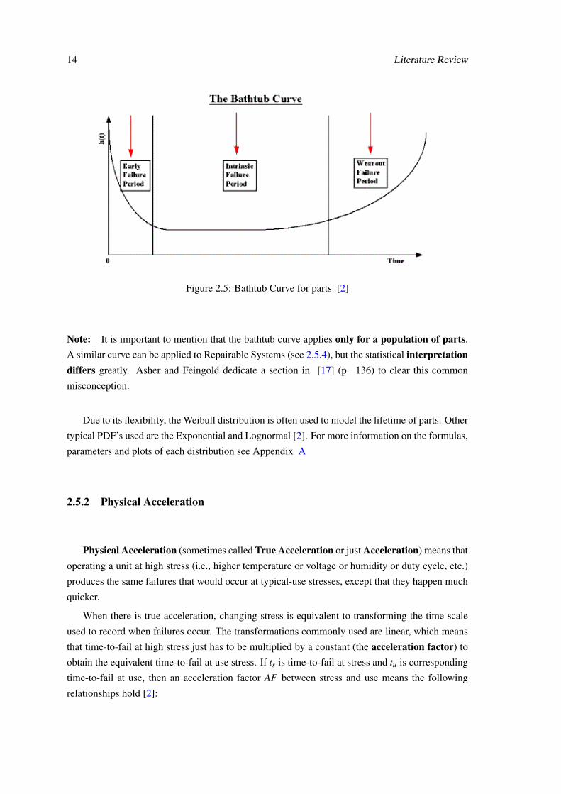
If enough parts from a given population are observed operating and failing over time, it is

relatively easy to compute periodic estimates of the failure rate h(t). It is common for the plot of

h(t) over time to yield a curve similar to the one in figure 2.5.

The initial region, Early Failure Period ( or Infant Mortality Period) that begins at t = 0

and is characterized by a high but rapidly decreasing failure rate. This behavior is attributed to

several factors that are related to manufacturing errors, imperfections, deviations from standards,

poor quality, and human factors.

Next, the failure rate levels off and remains roughly constant for the majority of the useful life

of the part. This is known as the Intrinsic Failure Period (also called the Stable Failure Period).

If parts from the population remain in use long enough, the failure rate begins to increase as

materials wear out and degradation failures occur at an ever increasing rate. This is the WearoutFailure Period.


Figure 2.5: Bathtub Curve for parts [2]

Note: It is important to mention that the bathtub curve applies only for a population of parts.

A similar curve can be applied to Repairable Systems (see 2.5.4), but the statistical interpretationdiffers greatly. Asher and Feingold dedicate a section in [17] (p. 136) to clear this common

misconception.

Due to its flexibility, the Weibull distribution is often used to model the lifetime of parts. Other

typical PDF’s used are the Exponential and Lognormal [2]. For more information on the formulas,

parameters and plots of each distribution see Appendix A

2.5.2 Physical Acceleration

Physical Acceleration (sometimes called True Acceleration or just Acceleration) means that

operating a unit at high stress (i.e., higher temperature or voltage or humidity or duty cycle, etc.)

produces the same failures that would occur at typical-use stresses, except that they happen much

quicker.

When there is true acceleration, changing stress is equivalent to transforming the time scale

used to record when failures occur. The transformations commonly used are linear, which means

that time-to-fail at high stress just has to be multiplied by a constant (the acceleration factor) to

obtain the equivalent time-to-fail at use stress. If ts is time-to-fail at stress and tu is corresponding

time-to-fail at use, then an acceleration factor AF between stress and use means the following

relationships hold [2]:


Time-to-Fail: tu = AF× ts

Failure Probability: Fu(t) = Fs(t/AF)

Reliability: Ru(t) = Rs(t/AF)

Failure Rate: hu(t) = (1/AF)hs(t/AF)

PDF : fu(t) = (1/AF) fs(t/AF)

A model that predicts time-to-fail as a function of stress is an Acceleration model. If t f =

G(S), with G(S) denoting the model equation for an arbitrary stress level S, then the acceleration

factor between two stress levels S1 and S2 can be evaluated simply by AF = G(S1)/G(S2). [2]

Acceleration models are usually based on the physics or chemistry underlying a particular

failure mechanism.

Two of the most common acceleration models are presented in the next sections. These two

models as well as several others are described in [2].

2.5.2.1 Arrhenius

The Arrhenius model predicts failure acceleration due to temperature increase. It takes the form [2]:

t f = A · exp[

∆HkT

], (2.11)

where

• T is the temperature measured in degrees Kelvin at the point when the failure process takes

place

• k is Boltzmann’s constant (8.617e-5 in ev/K)

• A is a scaling factor that drops out when calculating acceleration factors

• ∆H is the activation energy, which is the critical parameter in the model

The acceleration factor between a higher temperature T2 and a lower temperature T1 is given

by

AF = exp[

∆Hk

(1T1− 1

T2

)]. (2.12)


2.5.2.2 Eyring

The Eyring model has a theoretical basis in chemistry and quantum mechanics and can be used

to model acceleration when many stresses are involved. The model for temperature and one addi-

tional stress takes the general form:

t f = AT αexp[

∆HkT

+

(B+

CT

)·S1

], (2.13)

where,

• S1 could be any relevant stress, like voltage or current

• α,∆H,B and C determine acceleration between stress combinations

• k as with the Arrhenius model, is the Boltzmann’s constant and temperature is in degrees

Kelvin.

Another non-thermal stress term can be added, hence the model becomes:

t f = AT αexp[

∆HkT

+

(B+

CT

)·S1 +

(D+

ET

)·S2

], (2.14)

2.5.3 Bottom-up approach to System Reliability

Several simple models and methods can be used to compute system reliability, starting with

failure rates for failure modes within individual system parts and component configurations. Dif-

ferent component configurations means different system reliability. The configuration models

presented in this reference are:

• Competing Risk Model;

• Series configuration;

• Parallel configuration;

• r out of n Model;

• Complex Model.

The schematics of each configuration, as well as its

2.5.3.1 Competing Risk Model

Assume a (replaceable) component or part has k different ways it can fail. These are called failuremodes and underlying each failure mode is a failure mechanism.

The Competing Risk Model evaluates component reliability by "building up" from the relia-

bility models for each failure mode. It is applicable when the following conditions are met:


• Each failure mechanism leading to a particular type of failure (i.e., failure mode) proceeds

independently of every other one, at least until a failure occurs;

• The component fails when the first of all the competing failure mechanisms reaches a failure

state;

• Each of the k failure modes has a known life distribution model Fi(t).

If c refers to the component and i to the i-th failure mode, then then the competing risk model

formulas are [2]:

Rc(t) =k

∏i=1

Ri(t)

Fc(t) = 1−k

∏i=1

[1−Fi(t)]

hc(t) =k

∑i=1

hi(t)

2.5.3.2 Series Model

The Series Model is used to build up from components to sub-assemblies and systems. It only

applies to non replaceable populations (or first failures of populations of systems). The assump-

tions and formulas for the Series Model are identical to those for the Competing Risk Model, with

the k failure modes within a component replaced by the n components within a system. [2]

The following three assumptions are needed:

• Each component operates or fails independently of every other one, at least until the first

component failure occurs;

• The system fails when the first component failure occurs;

• Each of the n (possibly different) components in the system has a known life distribution

model Fi(t).

If the Series Model assumptions hold, then [2]:

RS(t) =n

∏i=1

Ri(t)

FS(t) = 1−n

∏i−1

[1−Fi(t)]

hS(t) =n

∑i=1

hi(t)


with the subscript S referring to the entire system and the subscript i referring to the i-th

component. Note that the above holds for any arbitrary component life distribution models, as

long as "independence" and "first component failure causes the system to fail" both hold.

2.5.3.3 Parallel Model

The opposite of a series model, for which the first component failure causes the system to fail, is

a parallel model for which all the components have to fail before the system fails. If there are n

components, any (n− 1) of them may be considered redundant to the remaining one (even if the

components are all different). When the system is turned on, all the components operate until they

fail. The system reaches failure at the time of the last component failure.

The assumptions for a parallel model are:

• All components operate independently of one another, as far as reliability is concerned;

• The system operates as long as at least one component is still operating. System failure

occurs at the time of the last component failure;

• The CDF for each component is known.

For a parallel model, the CDF FS(t) for the system is just the product of the CDFs Fi(t) for the

components, or [2]

FS(t) =n

∏i=1

Fi(t) .

RS(t) and hS(t) can be evaluated using basic definitions, once FS(t) is known.

2.5.3.4 R out of n model

An "r out of n" system contains both the series system model and the parallel system model as

special cases. The system has n components that operate or fail independently of one another and

as long as at least r of these components (any r) survive, the system survives. System failure occurs

when the (n− r+1)-th component failure occurs.

Whenr = n, the r out of n model reduces to the series model. When r = 1, the r out of n model

becomes the parallel model.

The simple case where all the components are identical is treated here.

Formulas and assumptions for the r out of n model (identical components):

• All components have the identical reliability function R(t).

• All components operate independently of one another (as far as failure is concerned).

• The system can survive any (n−r) of the components failing. The system fails at the instant

of the (n− r+1)-th component failure.

2.6 Overall Equipment Effectiveness 19

System reliability is given by adding the probability of exactly r components surviving to time

t to the probability of exactly (r + 1) components surviving, and so on up to the probability of all

components surviving to time t. These are binomial probabilities (with p = R(t)), so the system

reliability is given by [2]:

RS(t) =n

∑i=r

(n

i

)[R(t)]i [1−R(t)]n−i .

2.5.3.5 Complex Systems

Many complex systems can be diagrammed as combinations of Series components, Parallel com-

ponents, R out of N components and Standby components. By using the formulas for these models,

subsystems or sections of the original system can be replaced by an "equivalent" single component

with a known CDF or Reliability function. Proceeding like this, it may be possible to eventually

reduce the entire system to one component with a known CDF [2].

2.5.4 Basic Models for Repairable systems

Asher and Feingold in [17] analyze Repairable Systems as stochastic point processes. A

stochastic point process is a mathematical model for a physical phenomenon characterized by

highly localized events distributed randomly in a continuum. Applied to repairable systems, the

continuum is time and the highly localized events are failures which are assumed to occur at

instants within the time continuum [18].

In [17] the following basic models (and variants) are discussed:

• Homogeneous Poisson Process (HPP);

• Non-Homogeneous Poisson Process (NHPP);

• Non-Homogeneous Poisson Process (NHPP);

• Branching Poisson Process (BPP);

• Renewal Process (RP);

• Superimposed Renewal Process (SRP).

For more information on the study of Repairable Systems as stochastic point processes, refer

to [17], [19] and [18].

2.6 Overall Equipment Effectiveness

Overall Equipment Effectiveness (OEE) is essentially the ratio of Fully Productive Time to Planned

Production Time. In practice, however, OEE is calculated as the product of its three contributing

factors:


OEE = Availability×Per f ormance×Quality (2.15)

In the context of OEE the three factors can be defined [20] as:

Availability is the ratio between the actual run time and the scheduled run time. The sched-

uled run time does not included breaks, lunches and other pre-arranged time a production line or

process may be down.

Availability =operating timescheduled time

(2.16)

Performance is the ratio between the actual number of units produced and the number of

unit that theoretically can be produced and is based on the standard rate. The standard rate is rate

the equipment is designed for.

Per f ormance =Parts Produced× Ideal Cycle Time

scheduled time(2.17)

Quality is the ratio between good units produced and the total units that were stated.

Quality =Units Produced−de f ective units

units produced(2.18)

2.7 Manufacturon

The XPRESS project [21] one of the projects that forms the basis for ReBORN, introduces the con-

cept of Manufactron. “A Manufactron is an agent based equipment which has all the knowledge

to perform a certain task, and that only needs to be told what and when to do it. This knowl-

edge based concept integrates the complete process chain: production configuration, multi-variant

production line and 100% quality monitoring.” [22]

2.8 Simulation

In order to tackle the challenges that come with the increasing complexity of modern manufac-

turing systems, such as resource and layout planning, simulation has been used successfully for

decades as a tool to support decision-making in this process with clear benefits, as it is cheaper and

2.8 Simulation 21

faster to build a virtual system and experiment with different scenarios and decisions before actu-

ally implementing it [23]. Simulation models can be classified according to several independent

pairs of attributes, such as:

• Stochastic or deterministic;

• Steady-state or dynamic;

• Continuous or discrete;

• Dynamic system simulation or dynamics simulation of field problems;

• Local or distributed.

For manufacturing systems simulation, one of the following three methods is used:[24]:

System Dynamics (SD) simulation

where the models are continuous based on differential or difference equations. The model

is represented in the form of causal loops and stock and flow diagrams with positive or negative

feedback relations. The mathematical equations can be exact, approximate or empirical. The

drawbacks are that it uses deterministic mathematical equations while the real world does not and

the structure of the system and the governing rules are constant [24].

Discrete Event Simulation (DES)

is the most widely used method for manufacturing systems simulation, the systems compo-

nents are modeled as objects with attributes. The states of the objects change in response to

specific events that can occur at random and several events can occur at the same time. The main

advantages of DES are [24]:

• the ease of use,

• the ability to include stochastic elements,

• the ability to track individual system components and get several performance measures for

them.

Agent Based simulation (ABS) is a particularization of DES, where agents, see 2.1.3.1,

are used instead of objects as the system components. The agents interaction with other agents

is described by simple rules but resulting into complex interactions. Their behavior can change,

based on their experience [24].


2.8.1 Limitation to current simulation techniques

There are two fundamental limitations to current simulation techniques, one of which being the

need for multiple simulation runs, which is not an issue when the decision maker is faced with few

scenarios to choose from, but can quickly escalate as the number of possible decisions increases,

for example: if the system consists of 10 components and each component has only two possible

alternatives, then there are 210 = 1024 alternatives to be simulated.

The other limitation is the impossibility to change the system under simulation. Although

some specific variables may be altered, overall the parameters and structure under simulation are

both static and rigid, much unlike real systems which are dynamic. [24]

2.8.2 Simulation Package

There are several simulation packages in the market, each with its own features and purposes. The

simulation software to be used in this project is Flexsim. It is a powerful discrete event simulation

(DES) software, that can be applied in many different fields, from manufacturing to logistics to

healthcare and others. The structure uses object-oriented design and objects are part of super-

classes, e.g. Fixed Resource - with objects like Processor, Sink and Source - or Task Executer -

with objects like Operator or Transporter. Flexsim has a 3D environment and its very easy to create

models by drag &dropping objects directly in them. Once the objects have been dropped into the

model they can then be edited via dialog box. The model can also be viewed in a hierarchical tree

view. It is possible for the user to create his own classes and libraries from scratch or customize

the existing ones.

The access to the data tree structure, makes it possible for the experienced user to interact with the

model via C++ or flexscript (Flexsim’s scripting language) in run-time. Flexsim models can be

saved in ".fsm" format or in a ".fsx" (a XML based format) file that can be edited directly (but not

in real-time).

There is the possibility to connect Flexsim to user developed DLL’s, which opens the way for ex-

ternal control in run-time via COM objects. Socket communication is also supported by Flexsim.

Figure 2.6 shows a 3D view of a model and some of the default libraries available on the left, from

where the user can drag the objects into the model.

2.9 Data Format for Information Exchange

XML has proven to be an effective method of transporting data from one location to another (W3C

2008). Data structure is its the main advantage. Its syntax allows storing each piece of data in user

defined markup tags. The markup tags are arranged in a hierarchy that represents the ordering of

the data in a parent/child relationship. XML is a neutral format that simplifies data sharing, data

transport, platform changes, and makes data more available. [25]

Data exchange standardization is adopting in many areas like process engineering, process control

2.9 Data Format for Information Exchange 23

Figure 2.6: Example of a production line model in Flexsim

engineering, oil and gas industry, and in manufacturing automation engineering. Two norms are

described in the following sections. [25]

2.9.1 AutomationML

Automation Markup Language (AutomationML) is a XML based neutral data format for storing

and exchanging plant engineering information. The aim is to interconnect the heterogeneous tool

landscape of engineering tools in mechanical plant engineering, electrical design, HMI develop-

ment, PLC, and robot control fields. AutomationML works as the glue between all the factory

planning tools. It implements an object oriented paradigm; real factory components are described

as data objects. They encapsulate different aspects of a real object. Typical factory components

are; geometry, kinematic behavior, classification within the factory topology, and the relations be-

tween the objects. There are already many industrial standards for many of those aspects. Within

AutomationML these standards are used and, if necessary, a standard enhancement is tried to be

developed. Basically AutomationML supports the following concepts:

• Factory topology - CAEX;

• geometry - COLLADA;

• Kinematic - COLLADA;

• behavior description - PLCOpen-XML, and references from CAEX to external data

2.9.2 Core Manufacturing Simulation Data

National Institute of Standards and Technology (NIST) researchers have been working on a stan-

dards development effort, Core Manufacturing Simulation Data (CMSD) under the guidelines,


policies and procedure of the Simulation Interoperability Standards Organization (SISO). The

work behind this paper relies on the CMSD Information Model. Due to a lack of interoperability

between manufacturing applications and simulation systems, the CMSD effort was launched. The

CMSD Information Model defines a data specification for efficient exchange of manufacturing

data in a simulation environment [25].

Chapter 3

Problem Analysis

The strategies and technologies to be developed during execution of ReBORN, will address rel-

evant issues in today’s manufacturing, such as the inability to re-use production equipment after

a production line is decommissioned, the lack of comprehensive design methodology for man-

ufacturing systems or the nonexistence of appropriate methods for dynamic cost assessment for

system design and system life-cycle optimization. It will use system information for real time

system adaptation and will take advantage of its use in improving overall system performance

throughout its life-cycle.

In this chapter the concept of VERSON is introduced, as well as the overall architecture of the

system under development in the Work Package 3 of ReBORN is presented, with special focus on

the subsystem being developed at FEUP.

3.1 VERSONs

The decision on the re-use of production equipment requires knowledge about the actual status

of the machine and its components after the past use and the adjustment and/or prediction of the

operating, service and maintenance characteristics, which have changed due to wear, exchange,

update and other influences during the past operation. In addition, information might be useful in

predicting possible changes of these characteristics during a foreseen operating period. The cre-

ation of this information requires an assessment of the operation so far (with the initial conditions

as a base line), which is characterized by the executed processes, the deployment conditions, the

supply data, sensor data, quality data and logs about failures, faults and service, maintenance and

calibration measures.

ReBORN will address these needs by the introduction of Versatile, Flexible and LyfecycleExtended Devices (VERSON)

25

26 Problem Analysis

VERSONs are agents which can have a physical or virtual representation of production equip-

ment. The virtual representation is mainly used for simulation purposes. In the physical represen-

tation, VERSONs wrap existing equipment and turn it into modular, agent-based, task-driven,

plug & produce devices for smart factories, which can be exchanged and adapted for both new

production goals and structures. The devices are always aware of their own state of capabilities

and remaining lifetime, which they offer to the production network.

The versons shall have:

• analytical capabilities to determine their own state, to find the best practical operational

parameters;

• intelligence to derive a lifetime prognosis, maintenance requirements, refurbishment plans;

• state-dependant cost model estimation related to:

– task execution

– maintenance

• communication capabilities to describe and optimize themselves towards their environ-

ment by providing knowledge and models about their properties, abilities, constraints and

re-use abilities (device self-description).

3.2 Overview of the High Performance Simulation Tool

In order to fulfill its vision, ReBORN will provide a high performance simulation tool, Figure 3.1,

with a dynamic self-learning environment and a modular structure. Each software module repre-

sents and simulates a specific production process under real conditions through the connection to

a knowledge database, including all the methods for the performance of this specific process.

The ReBORN method can be divided in two processes. The first is triggered when the user

defines a set of requirements and constraints for a production process. Those definitions are cap-

tured and the formalized job description is sent to the Layout Configurator, which will match the

requirements with the capabilities provided by VERSONs and other equipment to identify poten-

tial candidates to integrate the layout and will eliminate those that do not fit the constraints, like

size or geometry.

Once all the possible layouts have been configured, they are sent in AutomationML format,

see 2.9.1, to the Layout Simulator which will combine the results of three different assessments

and present the result back to the user, providing him with information for an educated decision in

designing the production line.

The knowledge from operational VERSONs and other equipment deployed in production en-

vironments is captured and used to update the VERSONs and the network so the models are

enhanced.

3.2 Overview of the High Performance Simulation Tool 27

Figure 3.1: ReBORN high performance simulation tool [3]

28 Problem Analysis

3.3 Problem specification

The part of ReBORN being developed at FEUP is framed in the subsystem outlined by the dashed

orange line in Figure 3.1 and it concerns the process of simulating the several layouts sent by the

Configurator and assessing their life-cycle impact.

The detail and amount of information available about the possible layouts and the VERSONs

that compose them will influence the the output, which is the result of three assessments:

• LCC (section 2.2);

• LCA (section 2.3);

• Reliability Assessment (section 2.4).

Here lies a key innovation in the design of manufacturing systems: the integration of reliabil-

ity and life-cycle status information in its conception.

The main results of the Reliability Assessment are a set of metrics, the most relevant being:

• Failure rate;

• MTBF;

• MTTR;

• Reliability;

• Availability;

• Performance;

• Quality;

• OEE.

The result of the LCC (concerning each machine) is:

• FV (Future Value)

• PV (Present Value)

• NPC (Net Present Cost)

• NPV (Net Present Value with initial costs)

3.3 Problem specification 29

The results obtained will be displayed in graphs by a web application, comparing the possible

layouts at machine level for each metric for a stronger visual impact on the user. Figure 3.2

shows an example of the comparison of the LCC assessment in two machines displayed in the

aforementioned tool. On the upper frame two machines are compared in terms of the NPV for a

period of two years and five years time. On the lower frame the same machines are compared for

the same period of time in terms of their FV, PV and NPC.

Figure 3.2: Example of a comparison of an LCC assessment in two machines

The work done for this thesis focuses on providing a tool to facilitate the creation of simulation

models of the layouts sent by the Layout Configurator, with the purpose of assessing their Relia-

bility. If the inputs are detailed enough, these models may also produce useful metrics in the study

of LCC and LCA.

30 Problem Analysis

Chapter 4

Machine Concept for the simulationmodels

Given that the purpose of this work is to provide a tool that facilitates the creation of simulation

models of the production lines sent by the Layout Configurator, with the main goal of assessing

the Reliability of these layouts, VERSONs (see 3.1) will be perceived as machines in a production

line and therefore only some of the VERSONs’ features are contemplated. Furthermore, at this

level of abstraction the actual jobs performed by the machines at tool level, like cutting or weld-

ing are not considered. The physical/geometrical representation of the model is not relevant for

the assessment either, so physical dimensions of the machines, their coordinates on the shopfloor,

the distances between workstations and other objects, the distances traveled by the product be-

ing assembled or produced, as well as the corresponding travel times are not considered in the

simulations.

It is also important to note that at the time of the realization of this work there was yet limited

information about the AutomationML structure adopted by the other partners in ReBORN and the

data contained in it, so assumptions were made as to what the inputs of the simulation were.

Over the next chapter, the models and concepts behind the individual machines /VERSONs

that make the production lines to be simulated, will be presented.

4.1 Machine as a system

Following the concepts introduced in 2.5.3, the machines will be modeled as systems com-

posed of any given number of parts and/or components, which are placed individually in sockets

(see 2.5). The components are arranged in a Series configuration 2.5.3.2, which means a ma-

chine fails when any component fails.

31

32 Machine Concept for the simulation models

4.1.1 Socket Level

When a component fails, it is replaced immediately with a new one of the same kind. In other

words, after each replacement the socket is put back into an "as good as new" condition. Each

component has a time-to-failure that is determined by the underlying distribution. Once again, a

distribution relates to a single failure (see 2.5.1) . The sequence of failures for the socket con-

stitutes a random process called a Renewal process (see 2.5.4). A renewal process is defined

as a nonterminating sequence of independent, identically distributed (IID) non-negative random

variables, X1,X2, ..., which with probability 1 are not all zero [17].

In figure 4.1, the component life is X j, and t j is the system time to the jth failure. Each

component life X j in the socket is governed by the same distribution F(x).

Figure 4.1: Illustration of Renewal Process [4]

4.2 Lifetime modeling

As already stated in previous sections, lifetime models apply only to the parts in sockets. The

following assumptions were made in regards to the models to be implemented in this solution:

• Lifetime will be accelerated or decelerated by load conditions referred to normal load con-

ditions. For the basic principles see 2.5.2;

• Physics of failure mechanism does not change under changed load conditions;

• The system under consideration exhibits cumulative damage, i.e. the remaining life depends

on future load and the future distribution function, starting at the previously accumulated

fraction of failure probability.

4.2.1 Lifetime distributions

Lifetime of parts can be modeled by any PDF, as explained in section 2.5.1. The most common

pdf used are the Weibull distribution and the Exponential distribution. Their formulas and plots

are presented in Appendix A.

4.2.2 Accelerated Lifetime models

4.2 Lifetime modeling 33

The concept of "physical acceleration" explained in 2.5.2 is used in these models, so that

higher loads imply faster equivalent time evolution (refered to normal load). This is explained

with the following example.

In figure 4.2 an example an evolution of step-load levels li over operating time is presented.

The normal load condition (reference) is l0. Acceleration factor is then:

AFi =li f e(lo)li f e(li)

Figure 4.2: Example of evolution of step-load levels over operating time

teq(t) is the equivalent lifetime, i.e. accumulated operating time weighted by acceleration

factors. It is given by:

When load conditions are arbitrary, ∆ti = ∆t, then teq(t) is

teq =∫ t

t0AF(t ′)dt ′

teq(t) contains the whole impact of historic load conditions.

Consider f (t) is a Weibull PDF (see A.2), with characteristic lifetime under normal load con-

ditions η0. The characteristic lifetime for arbitrary load conditions is given by:

η(t,L(t)) =η0

AF(t,L(t))

Figure 4.3 depicts the equivalent failure probability, when 3 different load conditions are ex-

perienced over the operating time.

34 Machine Concept for the simulation models

Figure 4.3: Equivalent failure probability with 3 different load conditions

From figure 4.3, it is possible to derive

F1(s) = F(tnow) = Fnormal(teq)

4.2.3 Lifetime information

For each failure mode, the following should be provided:

• t0 - operating time at last repair, maintenance, replacement or birth;

• teq,0 - describes pre-damage at t0;

• teq - describes accumulated history;

• AFm(t,Lm)Mm=1 - functional or numerical representation of acceleration factors for every load

variable Lm; includes normal load conditons;

• PDF and parameters under normal load conditions for each component.

Chapter 5

Implementation

One of the obstacles in the usage of simulation models as a "decision support system" when

planning the layout of a new production line, is that the creation of these models is time consuming

and prone to errors. The work developed under this thesis (see 3.3) tackles this issue.

This Chapter describes the implementation of the tool that facilitates and automatizes the pro-

cess of creating simulation models (conceptualized in Chapter 4) of the production lines in the

context of ReBORN (see 3) and the integration of Flexsim (see 2.8.2) with the layout description

in XML.

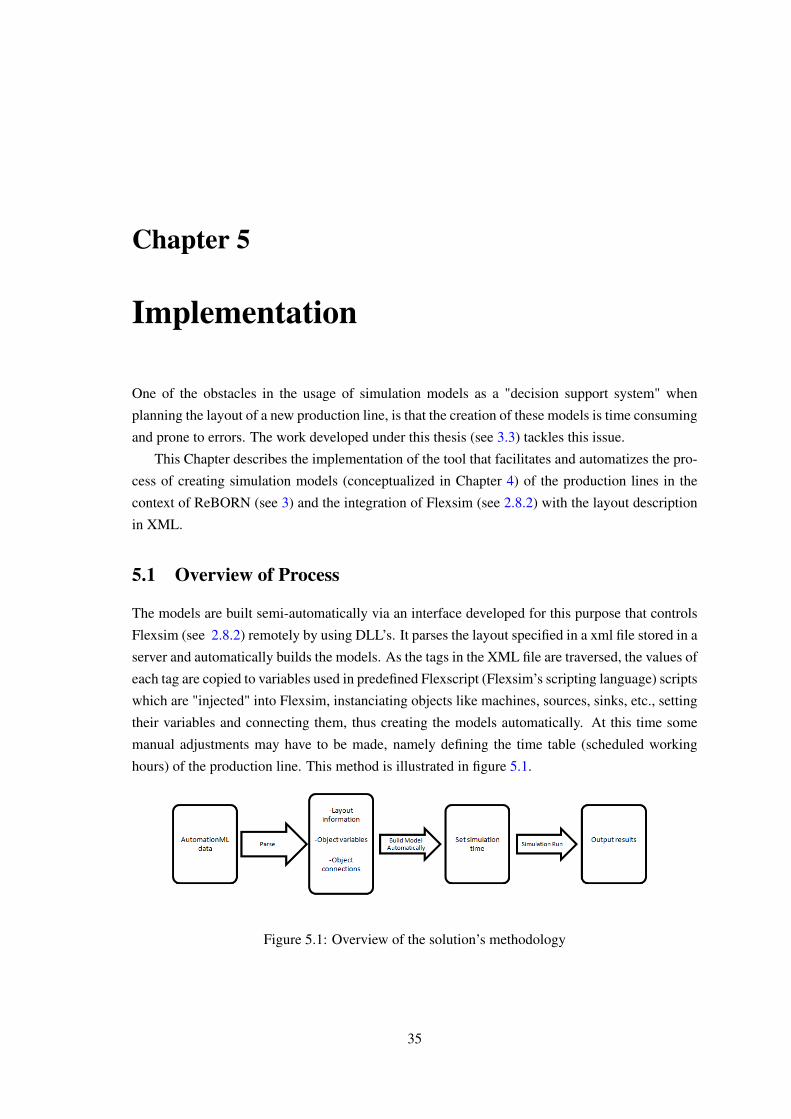
5.1 Overview of Process

The models are built semi-automatically via an interface developed for this purpose that controls

Flexsim (see 2.8.2) remotely by using DLL’s. It parses the layout specified in a xml file stored in a

server and automatically builds the models. As the tags in the XML file are traversed, the values of

each tag are copied to variables used in predefined Flexscript (Flexsim’s scripting language) scripts

which are "injected" into Flexsim, instanciating objects like machines, sources, sinks, etc., setting

their variables and connecting them, thus creating the models automatically. At this time some

manual adjustments may have to be made, namely defining the time table (scheduled working

hours) of the production line. This method is illustrated in figure 5.1.

Figure 5.1: Overview of the solution’s methodology

35

36 Implementation

5.2 Data Structure

AutomationML was the data format adopted to be used across all levels of hierarchy of the

project’s solution. Because it is a standardized data format and the structure to be used was yet to

be defined by the other partners upstream in ReBORN at the time of the writing of this dissertation,

another XML format was used for the development and experiments. An example is shown in

Figure 5.2.

The structure is kept simple for development and experiments and only the necessary infor-

mation for the layout is represented since additional tags with other information can be ignored.

In Figure 5.2, the layout described consists of 3 machines: M1, M2 and M3 a source (Source1)

from where parts or products enter the model and a sink (Sink1) where the final product exits the

model. The inputs of the machines are: Name, Setup Time, Cycle-time, MTBF and MTTR. The

child element of <Sequence> - <pair> - describes the connections between objects in the model.

5.2 Data Structure 37

Figure 5.2: Example of a layout defined in XML

38 Implementation

5.3 Flexsim Remote Control

The process of creating simulation models is time consuming and error-prone. Therefore, finding

a way to (1) automate this process and (2) make the simulation software "invisible" to the user was

essential. In order to achieve these two goals it was necessary to control the simulation software

and the models externally. This was the most difficult part of the work and where most of the time

was spent.

5.3.1 Explored alternatives

While a lot of capability exists in Flexsim, knowledge is still limited in various areas as to control-

ling it remotely. Several ways were explored to meet the objectives:

• Sockets;

• CMSD; see sec. 2.9.2

• using .fsx;

• Microsoft Excel;

• use of DLL’s;

• Batch Files and VBS/VBA command-line execution;

• Component Object Model.

As stated in section 2.8.2 Flexsim supports socket communication; however, documentation is

scarce and no examples were found to use as a starting point. Another method tried was through

the execution of shell commands to open a Flexsim model and passing command-line parameters

through the shell that the Flexsim model could interpret and make decisions from, using .bat files,

VBScript or VBA, but these proved to be ineffective. Flexsim allows the connection to user made

DLL’s and this was tried as a method to remotely pass parameters into a model but was inefficient.

Another failed approach was through Excel tables that the Flexsim model would extract values

from, but was inefficient and the amount of variables and their complexity would rapidly escalate,

making it impossible to use. Several mentions to the use of CMSD 2.9.2 in automatically generat-

ing the Flexsim model [26] [27] [28] were found, but these would still require a translator for the

corresponding XML format which was not available.

The use of Flexsim’s XML based format (.fsx) was examined also. It proved easy to in-

sert objects like machines or conveyors in the model, but the main problem was in following the

logic behind the notation that set the connections between object models, making it impossible

to connect all the objects correctly. It also did not allow for run-time model editing, since any

modifications to the .fsx file would implicate the closing of the model and its re-opening. Another

5.4 Interface 39

disadvantage of this method is that sometimes its necessary to edit multiple nodes when a simple

command line in Flexscript or C++ would do it.

5.3.2 Solution adopted

The solution adopted was the use of a Component Object Model (COM). A beta release of a COM

object for Flexsim 4 was made available by Flexsim developers. The initial project was created

with C++ in Visual Studio 2008 for 32bit platforms. The project had numerous bugs that were

preventing it from compiling successfully. Once the source code was debugged and other changes

were made to adapt it to newer versions of Flexsim, namely the Registry Key for Flemxsim 4 to

the version in use, the object worked as expected. Initally, Flexsim 5 had to be used instead of the

latest release, Flexsim 7.5, due to abnormal behavior observed on the Flexsim model when testing

the COM object with Flexsim 7.5. As development continued and a more basic use of the COM

was adopted, simply using it to "inject" scripts instead of directly changing the nodes in Flexsim’s

model data tree, the use of Flexsim 7.5 was successful.

From the Client side, some of methods can be called that make it possible to access and edit

the model data tree in run-time. Most of these methods mimic Flexscript (Flexsim’s scripting lan-

guage) commands. Given that the COM is only a beta version, the number of methods that can

access the model data tree is very limited in comparison with all the Flexscript commands. This

limitation is overcome by using a particularly useful method FlexsimAXApp::ExecuteString(BSTR

execString, double* retval) which executes the string passed as parameter on the Flexsim model

as Flexscript, basically allowing for any Flexscript command to be called remotely.

Apart from the methods that mimic Flexscript, other methods that are called from the client

side worth of notice:

• FlexsimAXApp::StartApplication(BOOL) - opens a new Flexsim thread;

• FlexsimAXApp::ExitApplication(void) - kills the FLexsim thread;

• FlexsimAXApp::OpenLibrary(BSTR path) - opens a Flexsim library specified in the path;

• FlexsimAXApp::OpenModel(BSTR path) - opens the Flexsim model specified in the path.

Before using the COM, the Client DLL has to be registered through the command line.

5.4 Interface

An HTML page was created as the interface to link all the components of the solution together.

This web page will, from now on, be called Interface. It uses the ActiveXObject in Javascript to

40 Implementation

interact with the COM object and call the methods on the client side. Due to the use of ActiveX,

a Microsoft’s proprietary software framework, the web page only works with Microsoft’s Internet

Explorer.

Once the Interface is open, the user can start a new instance of Flexsim, which will open a

Flexsim user library as well, that has some components of the COM server installed, as well as

other elements used for the simulation models described in the next section. This instance serves

as a foundation on which the user will work, either by opening other saved models, using Flexsi-

mAXApp::OpenModel(BSTR path), inserting objects in the model individually and connecting

them or by building the model from a description in a XML file.

5.4.1 Overview of the Interface

Interaction with the Interface is kept simple, buttons and html <textarea> for passing parameters

are the only forms of user interaction with it.

All the functions and logic of the Interface were written in Javascript. The methods from

the COM object that control Flexsim remotely are instantiated inside Javascript functions that are

called by the user when certain buttons are pressed. Early in the development of the Interface,

instantiation of Flexsim objects in the model was done "manually", where the user would submit a

form with the input data in the <textarea>. Several functions were built to implement the different

objects. They were later used to instantiate objects taking node values of a XML file as parameters.

Some functions combine the instantiation of multiple objects. For instance, when inserted in-

dividually, objects of the class FixedResource (see 2.8.2) (e.g. Processors, i.e. machines) cannot

simulate breakdown events. Another object - MTBF/MTTR - has to be instanciated, where the

MTBF and MTTR are defined. These MTBF/MTTR objects can have several members (other

objects like Processors) and each member may belong to other MTBF/MTTR objects. In this so-

lution, when each machine is added to the model, a MTBF/MTTR object, of which the machine is

a member, is added automatically as well.

Due to the limited number of methods implemented on the COM Client and the difficulty

of implementing new ones, the method FlexsimAXApp::ExecuteString(BSTR execString, dou-

ble* retval) was used to overcome this since it executes the string it receives as a parameter as

Flexscript. In other words, it allows the "injection" of Flexscript into the model, just like running

a script with Flexsim’s script console. This function was used in fact to implement a Flexscript

console in the Interface, particularly useful during development as the console in the software is

only available when the licenses are activated.

5.4 Interface 41

5.4.2 Automatic model generation from XML

This is one of the most important features of the Interface, as it solves the problem of building

the model manually which is, as stated in sec. 5.3, a time consuming and error-prone process. For

security reasons client-side Javascript cannot access the localhost, so the XML files were stored in

FEUP’s SAMBA server during development.

All modern browsers have a built-in XMLHttpRequest object to request data from a server.

One of the characteristics of this object is that it enables the possibility to request and receive

data from a server without reloading the page. One of the properties of XMLHttpRequest is

the responseXML. This property returns the response as a XML DOM object. A XML DOM

(Document Model Object) is a standard programming interface for XML and it defines a standard

way for accessing and manipulating XML documents.

In the Interface, xmlhttp is an instance of XMLHttpRequest. When xmlhttp.responseXML is

called, the result is a XML DOM named xmlDoc, which is traversed and the node values are passed

as parameters in the same functions created in early stages of the development of the Interface,

that allow the instantiation of several types of objects in the model and their connection. Figure 5.3

shows the model created by the Interface with the layout defined in the XML of Figure 5.2.

Figure 5.3: Example of a layout defined in XML

It should be noted that the display of the objects in the 3D view of Figure 5.3 was altered man-

ually for illustration purposes. When objects are instantiated they are all in the location (0,0,0). As

stated in Chapter 4 the physical location of the machines is not relevant in this context; however,

placing the object in the right coordinates if they are passed as input, could be easily done with a

simple script.

42 Implementation

5.5 Flexsim Models

In order to implement the simulation models that realize the concept in Section 4 for the

machines, the use of several Flexsim objects has to be combined. Also, given that the concept is

the same for all the machines, the standard machines in Flexsim (the Processors) were edited and

saved in a user library so they can be re-utilized.

Standard objects in Flexsim come with very little features. The basic Processor allows the user

to define a setup time and a cycle time. All the other features have to be added to the objects, like

labels to store values, what actions to execute on each trigger etc.

5.5.1 Basic Flexsim concepts

5.5.1.1 Labels

Any number of labels can be defined for any object. Labels can of type number or string. Labels

can be set at any time. In this case for each machine a number of labels where added, some of

them are used to increment the value of a metric, like the number of breakdowns, or number of

good or bad pieces produced in each machine. Other labels are useful when defining the logic of

the events or actions to perform at any given time.

The basic labels to store values of metrics in a machine are:

• good pieces produced;

• bad pieces produced;

• number of breakdowns;

If more than one type of pieces or products are produced, then each product or piece (Flowitem)

has its own type number, stored in a label as well. This allows, for example, the machines to keep

track of how many pieces of each type were produced and define different cycletimes for each

type of Flowitem.

5.5.1.2 Triggers

Each object has a different set of predefined triggers. Triggers allow an increase in complexity in

the models. When a certain event happens (triggered), the functions associated with that event are

called. Triggers for the machines are:

• On Reset;

• On Message;

• On Entry;

• On Exit;

5.5 Flexsim Models 43

• On Setup Finished;

• On Process Finish.

5.5.1.3 Breakdowns

Breakdowns in machines are modeled with a special kind of object called "MTBF/MTTR" ob-

jects. Each "MTBF/MTTR" can have many different machines as its members, and each machine

can have several "MTBF/MTTR" associated with it. The inputs of these objects are :

• First Failure Time;

• MTBF;

• MTTR;

Note: The notation MTBF and MTTR used in these objects is misleading, as it defines the

time to the next failure and time to the next repair and not Mean Time Between Failures and

Mean Time to Repair.

The triggers associated with these objects are:

• On BreakDown;

• On Repair.

5.5.2 Implemented Models

When the model is created and objects instantiated the values for cycletime, setup time, qualityfactor for each machine are defined as well. For each itemtype (given by the type number label of

a Flowitem) different cycle times and quality factors may be defined.

When the model is running and an item enters a machine, the sequence of steps are as follows:

• OnEntry trigger the machine reads the Flowitem’s type number label;

• It then processes the item for the duration of the cycletime as defined;

• OnProcessFinish, it performs a Bernoulli test, where, with a certain probability (given by

the quality factor) it may change the item type number, meaning the process produced a

defect and the Flowitem will be rejected;

• OnExit, if itemtype == 2, meaning the item is not good, the itemtype exits the system

through a special Sink. If itemtype! = 2, then it proceeds to the next machine.

44 Implementation

OnExit, labels that keep record of produced pieces (good or bad) are incremented. OnReset

Good pieces label, Bad pieces label and Number of breakdowns labels are set to 0.

On the model data tree, a record is kept of the time spent by the machine in each state. There

are 50 different states that is kept a record e.g. Processing Time, Scheduled downtime, Breakdown

time or Setup time.

5.5.2.1 Breakdowns in the implemented models

From the concept explained in Chapter 4, each machine is composed of several sockets, each

socket has a part or component and they are arranged in a series configuration.

This can be modeled with the "MTBF/MTTR" objects presented in 5.5.1.3, where each socket

is represented by one "MTBF/MTTR" object. The lifetime distribution of its parts is directly de-

fined in the input MTBF of the object. The value in this input is given by a function that returns a

random number with the PDF and the parameters defined. In each new cycle (meaning a part has

died and was replaced) a new value for the next time-to-failure is generated, just like in Chapter 4.

OnBreakdown, the Number of Breakdowns label for that machine is incremented.

5.5.3 Shortcomings in the implementation

The solution implemented to simulate the behaviour of the sockets, does not include the acceler-

ated lifetime, as described in section 4.2.2.

The reason is that the input MTBF in the "MTBF/MTTR" object is read at every OnRepair

trigger and although the value can be altered in the input, it will not be read until the next OnRe-

pair trigger. Several ways to force the OnRepair trigger were attempted, but were not successful.

The only viable alternative explored would be to change the models entirely, instead of "MTBF/MTTR"

objects create a User event for each socket that:

• periodically performs a Bernoulli test (B(F,1,0)) which has probability F of retuning 1;

• if B(F,1,0) == 1 then the event sends a message (sendmessage()) and a delayed message

(senddelayedmessage()) to the machine;

• OnMessage (the machine receives the first message) execute stopobject();

• OnMessage (the machine receives the delayed message) execute resumeobject().

Probability F is the CDF (F(t)) of the lifetime distribution for that socket, with t = teq and the

parameters of the PDF are updated to the corresponding load level 2.5.2.

Moreover, this solution implies a change in the way labels of the machine are incremented.

Instead of using OnRepair and OnBreakdown (current solution) labels would have to be updated

OnMessage.

Due to lack of time these changes were only studied, but not implemented.

5.5 Flexsim Models 45

5.5.4 Outcome of the Simulations

From the values stored in the labels, and the internal variables of the machines that record the time

spent in each state (accessible in the model data tree), the following results can de computed for

each machine:

• Planned Production Time (hours/year);

• Current Planned Production Time (hours);

• Current Operating Time (h);

• unscheduled Down Time year;

• Cycletime (per itemtype) (average);

• Combined Cycletime (average);

• No. Good Pieces (per itemtype) ;

• No. Good Pieces total;

• No. Bad Pieces (per itemtype) ;

• No. Bad Pieces total;

• Quality factor (per itemtype) ;

• Quality factor (total);

• No. machine failures;

• No. repairs (per socket);

• Total Power Consumed (MW);

• Availability;

• Performance;

• Quality;

• OEE.

46 Implementation

Chapter 6

Conclusions and Future Work

This chapter concludes the thesis. A brief review on the developed work and the results it

achieved is contained in it. At the end of this chapter some suggestions for further research are

exposed.

6.1 Conclusions

This dissertation was framed in the context of ReBORN project, which envisions the demon-

stration of strategies and technologies that support the a new paradigm fo re-use of production

equipment in old, renewed and new factories.

A simulation tool is being developed by several partners in the project which will allow for the

integration of reliability and life-cycle status information early in the conception of manufacturing

systems.

The purpose of the work developed for the thesis, was to provide a tool to facilitate the creation

of simulation models of production line layouts, with the purpose of assessing their Reliability.

The first step into the development of this tool was to find a way to control Flexsim - the

simulation software- remotely. This is done via a COM object. The Interface was developed in

HTML/Javascript since they support COM objects.

The next step was to automate the process of building simulation models. Given that the infor-

mation about the production layouts comes in a XML file, the Interface makes a xmlHttpRequest

to the server where file is stored. The resulting XML DOM is traversed and the values in the

nodes are the parameters of functions developed in the previous step, that instantiate objects in the

simulation model.

The third step was perfecting the models on Flexsim. A new Flexsim object was created and

added to a user library, the SuperProcessor. It keeps record of the number of Good and Bad parts

produced, as well as the number of breakdowns it experienced. The SuperProcessor also has some

built-in logic to handle the effects of defects or losses upstream in the production line.

47

48 Conclusions and Future Work

The biggest difficulty encountered during the development, and where most of the time was

spent, was on the first step - external control of Flexsim. Several technological options were tested

but none worked.

The choice for HTML and Javascript limits the Interface, since for security reasons modern

browsers do not allow access across domains.

The methodology proposed is valid in the context of ReBORN and the automatic model gen-

eration was implemented successfully; however, further tests with a suitable validation scenario

have to be conducted before the models on the Flexsim side can be formally validated.

6.2 Future Work

Further developments can be de done to this work. For one hand, the continuation of this solution

starting by validating the proposed models for Flexsim. The Interface can have installed the fea-

ture of generating a XML file with the results of the assessment.

The shortcomings exposed in 5.5.3 should be implemented, so that the simulation models are

accurate and coherent with their concept.

The models proposed will have to be review to adapt to the inputs when the AutomationML

the structure is defined by the other partners.

A different approach to the solution could be taken however, by translating the AutomationML

files to .fsx (Flexsim XML) and creating the simulation models directly. This solution could

increase the variety of the models; on the other hand, the complexity of changing all the nodes

required in the Flexsim XML tree may render it impractical, as sometimes changing an object

alters the structure of other objets in the tree.

Appendix A

Common formulas and plots for lifetimemodels

Formulas and plots in this Appendix from [2]

A.1 Exponential

The exponential model, with only one unknown parameter, is the simplest of all life distribution

models. The key equations for the exponential are shown below: [2]

PDF: f (t,λ ) = λe−λ t

CDF: F(t) = 1− e−λ t

Reliability: R(t) = e−λ t

Failure Rate: h(t) = λ

Cumulative Hazard Rate: H(t) = λ t

MTTF: 1λ

Median: ln2λ∼= 0.693

λ

Variance: 1λ 2

Note that the failure rate reduces to the constant λ for any time. The exponential distribution

is the only distribution to have a constant failure rate.

The plots for the exponential PDF and CDF are shown in figures A.1 and A.2 respectively.

49

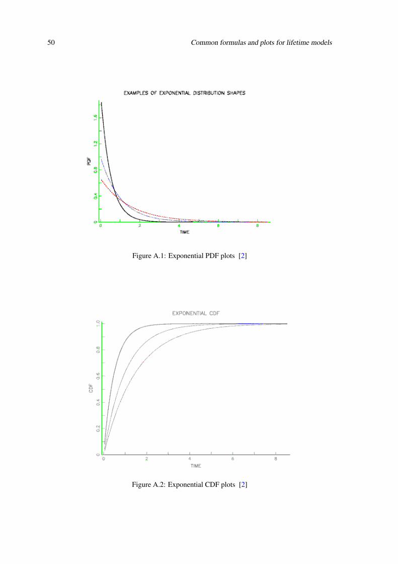
50 Common formulas and plots for lifetime models

Figure A.1: Exponential PDF plots [2]

Figure A.2: Exponential CDF plots [2]

A.2 Weibull 51

A.2 Weibull

The Weibull is a very flexible life distribution model with two parameters. Its CDF and PDF

and other key formulas given by: [2]

PDF: f (t,β ,η) = β

t

(tη

)β

e−(tη )

β

CDF: F(t) = 1− e−(tη )

β

Reliability: R(t) = e−(tη )

β

Failure Rate: h(t) = β

η

(tη

)β−1

Cumulative Failure Rate: H(t) =(

tη

)β

Mean: ηΓ

(1+ 1

β

)Median: η(ln2)

1β

Variance: η2Γ

(1+ 2

β

)−[ηΓ

(1+ 1

γ

)]2

with η the Scale parameter (the Characteristic Life), β the Shape Parameter, and Γ is the

Gamma function with Γ(N) = (N−1)! for integer N.

A more general three-parameter form of the Weibull includes an additional waiting time pa-

rameter γ (sometimes called a shift or location parameter). The formulas for the 3-parameter

Weibull are easily obtained from the above formulas by replacing t by (t− γ) wherever t appears.

No failure can occur before γ hours, so the time scale starts at γ , and not 0. If a shift parameter γ

is known (based, perhaps, on the physics of the failure mode), then all you have to do is subtract

γ from all the observed failure times and/or readout times and analyze the resulting shifted data

with a two-parameter Weibull. [2]

Special Case: When β = 1, the Weibull reduces to the Exponential Model, with η = 1/λ = the

mean time to fail (MTTF).

Depending on the value of the shape parameter β , the Weibull model can empirically fit a wide

range of data histogram shapes. This is shown by the PDF example curves in figure A.3.

From a failure rate model viewpoint, the Weibull is a natural extension of the constant failure

rate exponential model since the Weibull has a polynomial failure rate with exponent β −1. This

makes all the failure rate curves shown figure A.4 possible.


Figure A.3: Examples of Weibull PDF plots [2]

Figure A.4: Weibull Failure Rate plots for different values of β [2]

A.3 Lognormal 53

A.3 Lognormal

The lognormal life distribution, like the Weibull, is a very flexible model that can empirically fit

many types of failure data. The two-parameter form has parameters σ is the shape parameter and

T50 is the median (a scale parameter).

Note: If time to failure, t f , has a lognormal distribution, then the (natural) logarithm of time

to failure has a normal distribution with mean µ = lnT50 and standard deviation σ . This makes

lognormal data convenient to work with; just take natural logarithms of all the failure times and

censoring times and analyze the resulting normal data. Later on, convert back to real time and log-

normal parameters using σ as the lognormal shape and T50 = eµ as the (median) scale parameter.

Below is a summary of the key formulas for the lognormal.

PDF: f (t) = 1σt√

2πe−

( 12σ2

)(ln t− ln T50)

2

CDF: F(t) =∫ T

01

σt√

2πe−

( 12σ2

)(ln t− ln T50)

2

dt

F(t) = Φ

(ln t−ln T50

σ

)Φ(z) denotes the standard normal CDF.

Reliability: R(t) = 1−F(t)

Failure Rate: h(t) = f (t)R(t)

Mean: T50 e12 σ2

Median: T50

Variance: T 250 eσ2

(eσ2−1

)Note: A more general three-parameter form of the lognormal includes an additional waitingtime parameter θ (sometimes called a shift or location parameter). The formulas for the three-

parameter lognormal are easily obtained from the above formulas by replacing t by t−θ) wherever

t appears. No failure can occur before θ hours, so the time scale starts at θ and not 0. If a shift

parameter θ is known (based, perhaps, on the physics of the failure mode), then all you have to

do is subtract θ from all the observed failure times and/or readout times and analyze the resulting

shifted data with a two-parameter lognormal.


Examples of lognormal PDF and failure rate plots are shown below. Note that lognormal

shapes for small sigmas are very similar to Weibull shapes when the shape parameter β is large

and large sigmas give plots similar to small Weibull β ’s. Both distributions are very flexible and

it is often difficult to choose which to use based on empirical fits to small samples of (possibly

censored) data.

Figure A.5: Examples of Lognormal PDF plots [2]

A.3 Lognormal 55

Figure A.6: Examples of Lognormal Failure rate plots [2]

Appendix B

Schematics for bottom-up Reliability

Schematics presented in this Appendix from [2].

B.1 Series Model

Figure B.1: Example of a Series model [2]

57

58 Schematics for bottom-up Reliability

B.2 Parallel Model

Figure B.2: Example of a Series model [2]

B.3 Complex Model 59

B.3 Complex Model

Figure B.3: Example of a Complex model [2]

60 Schematics for bottom-up Reliability

Bibliography

[1] Reliasoft Corporation, System Reliability & Maintainability Reference. Tucson, Arizona:

ReliaSoft Publishing, 2015.

[2] M. Natrella, NIST/SEMATECH e-Handbook of Statistical Methods, C. Croarkin, P. Tobias,

J. J. Filliben, B. Hembree, W. Guthrie, L. Trutna, and J. Prins, Eds. NIST/SEMATECH,

2010. [Online]. Available: http://www.itl.nist.gov/div898/handbook/

[3] “Annex I – “Description of Work”. Project name: Innovative Reuse of modular knowledge

Based devices and technologies for Old, Renewed and New factories,” 2013.

[4] Reliasoft Corporation, Reliability Growth and Repairable System Analysis Reference.

Tucson, Arizona: ReliaSoft Publishing, 2015. [Online]. Available: https://books.google.pt/

books?id=iy9bQwAACAAJ

[5] Z. M. Bi, S. Y. T. Lang, W. Shen, and L. Wang, “Reconfigurable manufacturing systems: the

state of the art,” International Journal of Production Research, vol. 46, no. 4, pp. 967–992,

2008.

[6] M. G. Mehrabi, a. G. Ulsoy, and Y. Koren, “Trends and perspectives in flexible and recon-

figurable manufacturing systems,” Journal of Intelligent Manufacturing, vol. 13, no. 2, pp.

135–146, 2002.

[7] Y. Koren and M. Shpitalni, “Design of reconfigurable manufacturing systems,” Journal

of Manufacturing Systems, vol. 29, no. 4, pp. 130–141, 2010. [Online]. Available:

http://dx.doi.org/10.1016/j.jmsy.2011.01.001

[8] C. Christo and C. Cardeira, “Trends in Intelligent Manufacturing Systems,” Industrial Elec-

tronics, 2007. ISIE 2007. IEEE International Symposium on, pp. 3209–3214, 2007.

[9] A. Thomas, D. Trentesaux, and P. Valckenaers, “Intelligent distributed production control,”

Journal of Intelligent Manufacturing, vol. 23, no. 6, pp. 2507–2512, 2012.

[10] F. L. Almeida, B. M. Terra, P. Dias, and G. M. Goncalves, “Adoption Issues of Multi-agent

Systems in Manufacturing Industry,” Computing in the Global Information Technology (IC-

CGI), 2010 Fifth International Multi-Conference on, 2010.

61

http://www.itl.nist.gov/div898/handbook/

https://books.google.pt/books?id=iy9bQwAACAAJ

https://books.google.pt/books?id=iy9bQwAACAAJ

http://dx.doi.org/10.1016/j.jmsy.2011.01.001

62 BIBLIOGRAPHY

[11] W. Shen, Q. Hao, H. J. Yoon, and D. H. Norrie, “Applications of agent-based systems in

intelligent manufacturing: An updated review,” Advanced Engineering Informatics, vol. 20,

no. 4, pp. 415–431, 2006.

[12] M. Uppin and S. Hebbal, “Multi Agent System Model of Supply Chain for Information

Sharing,” Contemporary Engineering Sciences, vol. 3, no. 1, pp. 1–16, 2010. [Online].

Available: http://m-hikari.com/ces/ces2010/ces1-4-2010/uppinCES1-4-2010.pdf

[13] New South Wales Treasury, “Life Cycle Costing Guideline,” Total Asset Management, no.

September, p. 14, 2004.

[14] G. Rebitzer, T. Ekvall, R. Frischknecht, D. Hunkeler, G. Norris, T. Rydberg, W.-P.

Schmidt, S. Suh, B. P. Weidema, and D. W. Pennington, “Life cycle assessment:

Part 1: Framework, goal and scope definition, inventory analysis, and applications,”

Environment International, vol. 30, no. 5, pp. 701–720, 2004. [Online]. Available:

http://www.sciencedirect.com/science/article/pii/S0160412003002459

[15] a. Houshyar, “Reliability and Maintainability of Machinery and Equipment, Part 1: Accessi-

bility and Assessing Machine Tool R&M Performance,” International Journal of Modelling

and Simulation, vol. 24, no. 4, 2005.

[16] B. W. Torell and V. Avelar, “Mean Time Between Failure : Explanation and Standards,”

Power, vol. 78, pp. 1–10, 2004. [Online]. Available: http://support.casit.net/Portals/0/

NTForums_Attach/VAVR-5WGTSB_R0_EN.pdf

[17] H. Ascher and H. Feingold, Repairable Systems Reliability - modeling, inference, miscon-

ceptions, and their causes. New York : Marcel Dekker, 1984.

[18] O. Basile, P. Dehombreux, and F. Riane, “Identification of reliability models for non re-

pairable and repairable systems with small samples,” Proceedings of IMS 2004, 2004.

[19] B. H. Lindqvist, “Statistical Modeling and Analysis of Repairable Systems 2 \Major events

" in the history of repairable systems relia-,” pp. 1–18, 1997.

[20] “inductive automation - 3 Factors That Define OEE,” pp.

https://inductiveautomation.com/mes–software/oee–s. [Online]. Available: https://

inductiveautomation.com/mes-software/oee-software/oee-calculations/oee-definition

[21] “XPRESS Project.” [Online]. Available: http://www.xpress-project.eu/

[22] T. Ribeiro and G. Gonçalves, “Formal methods for reconfigurable assembly systems,” Pro-

ceedings of the 15th IEEE International Conference on Emerging Technologies and Factory

Automation, ETFA 2010, 2010.

[23] C. Jia, W. Ma, and X. Xia, “Research on modeling and simulating optimization for digital

factory,” 2010 International Conference on Measuring Technology and Mechatronics Au-

tomation, ICMTMA 2010, vol. 3, pp. 115–119, 2010.

http://m-hikari.com/ces/ces2010/ces1-4-2010/uppinCES1-4-2010.pdf

http://www.sciencedirect.com/science/article/pii/S0160412003002459

http://support.casit.net/Portals/0/NTForums_Attach/VAVR-5WGTSB_R0_EN.pdf

http://support.casit.net/Portals/0/NTForums_Attach/VAVR-5WGTSB_R0_EN.pdf

https://inductiveautomation.com/mes-software/oee-software/oee-calculations/oee-definition

https://inductiveautomation.com/mes-software/oee-software/oee-calculations/oee-definition

http://www.xpress-project.eu/

BIBLIOGRAPHY 63

[24] a. Seleim, A. Azab, and T. AlGeddawy, “Simulation methods for changeable

manufacturing,” Procedia CIRP, vol. 3, no. 1, pp. 179–184, 2012. [Online]. Available:

http://dx.doi.org/10.1016/j.procir.2012.07.032

[25] A. Boulonne and A. Skoogh, “Simulation Data Architecture for Sustainable Development,”

pp. 3435–3446, 2010.

[26] P. Barlas, G. Dagkakis, C. Heavey, B. Gaffney, P. Young, and J. Geraghty, “Test

Implementation and Initialisation of a Simulation model using CMSD,” Procedia CIRP,

vol. 25, no. Idm, pp. 276–282, 2014. [Online]. Available: http://dx.doi.org/10.1016/j.procir.

2014.10.039

[27] J. Fournier, “Model building with core manufacturing simulation data,” Proceedings - Winter

Simulation Conference, no. Wu 2005, pp. 2214–2222, 2011.

[28] S. Leong, Y. Lee, and F. Riddick, “A core manufacturing simulation data information

model for manufacturing applications,” Simulation Interoperability Workshop, Simulation

Interoperability and Standards Organization, pp. 1–7, 2006. [Online]. Available:

http://www.mel.nist.gov/div826/library/doc/sim_model.pdf




http://www.mel.nist.gov/div826/library/doc/sim_model.pdf

models for innovative factory layout design techniques and

Documents