monitoring k-nearest neighbor queries over moving objects · monitoring k-nearest neighbor queries...

Monitoring k-Nearest Neighbor Queries Over Moving Objects

Xiaohui Yu Ken Q. Pu Nick KoudasDepartment of Computer Science

University of TorontoToronto, ON, Canada M5S 3G4

{xhyu, kenpu, koudas}@cs.toronto.edu

Abstract

Many location-based applications require constant moni-toring of k-nearest neighbor (k-NN) queries over moving ob-jects within a geographic area. Existing approaches to thisproblem have focused on predictive queries, and relied onthe assumption that the trajectories of the objects are fullypredictable at query processing time.

We relax this assumption, and propose two efficient andscalable algorithms using grid indices. One is based onindexing objects, and the other on queries. For each ap-proach, a cost model is developed, and a detailed analysisalong with the respective applicability are presented. TheObject-Indexing approach is further extended to multi-levelsto handle skewed data.

We show by experiments that our grid-based algorithmssignificantly outperform R-tree-based solutions. Extensiveexperiments are also carried out to study the properties andevaluate the performance of the proposed approaches undera variety of settings.

1. Introduction

The prevalence of inexpensive mobile devices, such asPDA and mobile phones, and the wide availability of wire-less networks give rise to a new family of spatio-temporaldatabase applications. For example, in the location-basedmixed-reality games (e.g., BotFighters, BattleMachine),players with mobile devices locate and “shoot” other partic-ipants on city streets. In the location-based commerce set-ting, retail stores distribute e-flyers to potential customers’mobile devices based on their location.

In this paper we consider the problem of continuouslymonitoring multiple k-NN queries over moving objectswithin a two dimensional region of interest. Such queriesare important in many applications. In the gaming exam-ple, a player naturally wishes to keep track of the k near-byplayers in order to make a combat plan. In location-basedadvertising, in order to make the best use of available band-width, the stores may wish to send the e-flyers only to thecustomers who are currently closest to the store.

Given a set of objects, let P (t) ={p1(t), p2(t), . . . , pNp(t)} be their positions on a 2D

region as a function of time. The set of objects is highlydynamic: each object can move in an unrestricted fashion,i.e. we do not assume any pattern of motion. For a query setQ = {q1, q2, . . . , qNQ}, with each query being a static ormoving point in the same region, we are interested in moni-toring the exact k nearest neighbors (k-NNs) of each querypoint over time. Since we do not make any assumptions onthe trajectories of the objects, exact query answering canonly be done at the expense of some time-delay; i.e. at timet, the reported query answer is valid for the past snapshot ofthe objects and queries at time t − ∆t.

The problem of continously monitoring k-NN of movingobjects has been investigated in the past few years[1, 19, 13],with the emphasis on predicative or approximate query-answering by making assumptions on the motion patterns ofthe objects. This assumption is often violated in real appli-cations where the objects’ movements are non-predictable.Our work departs from the existing literature for that wemake no assumptions on the motion of the objects, and pro-vide the exact answers with a time delay (∆t).

In a continuous query-answering setting, the performanceis gauged by the rate at which query answers are generated,and this is dictated by the time delay (∆t). In order to im-prove the performance (i.e. reducing ∆t), we focus on de-signing index structures residing in main-memory.

We propose two methods to monitor k-NN queries overmoving objects. The first one is based on indexing the ob-jects themselves and we refer to it as Object-Indexing andthe second is based on indexing the queries and thus we re-fer to it as Query-Indexing. In both methods, the index takesthe form of a grid structure, which represents a canonicalpartition of the 2D space. The grid structure is preferableto other types of indices such as R-trees because its simplestructure lends itself to fast maintenance, which is a desiredproperty in the presence of highly dynamic data.

In the Object-Indexing method, two solutions are pro-vided for different scenarios. When the objects are knownto be uniformly distributed, an overhaul algorithm is usedto compute the k-NNs from scratch at each cycle. However,when there is no prior knowledge of the object distribution,or when the distribution is skewed, we show that an incre-mental approach can be taken. When there are only a smallnumber of queries, we find the Query-Indexing approachmore attractive than Object-Indexing. Analysis of all indices

Proceedings of the 21st International Conference on Data Engineering (ICDE 2005)

1084-4627/05 $20.00 © 2005 IEEE

and algorithms are provided and cost models are presented.We further extend the Object-Indexing method by using hi-erarchical grids to avoid performance degradation when thedistribution of moving objects is skewed.

Our contributions are summarized as follows:

• Computing k-NN, in two ways, by using a dynamicallyupdated grid-based index structure to index objects orqueries.

• Generalizing the object indices to hierarchical struc-tures. This is shown to improve query performance androbustness for skewed object distributions.

• Extending the query processing to incrementally main-tain the query answers. This further improves the per-formance when the objects’ movement is localized, i.e.the velocity is in general bounded.

• A theoretical analysis of the two types of indexing(object-index and query index) w.r.t. uniform andskewed object distributions. A somewhat surprising re-sult is that the k-NN query answering can be done withconstant-time (i.e. independent on the number of ob-jects) when the objects are uniformly distributed.

• Experimental validation of the theoretical analysis andevaluation of the hierarchical and incremental exten-sions. We simulated on both synthetic data as well asdata generated based on the Chicago area roadmap. Wealso performed a comparative study of our approachwith R-tree and its variants, and conclude that in thehighly dynamic setting, our approach out-performs treebased indexes by many folds.

The rest of the paper is organized as follows. Section 2surveys related work. Section 3 describes how to solve thek-NN search problem through object-indexing and query in-dexing, while Section 4 presents their hierarchical exten-sions. Section 5 shows the experimental results, and Sec-tion 6 concludes this paper.

2. Related Work

Answering k-nearest neighbor queries is a classicaldatabase problem. Traditionally, research on this prob-lem has focused on static objects. Most methods use in-dices built on the data to assist the k-NN search. Perhapsthe most widely used algorithm is the branch-and-boundalgorithm[14] based on R-trees[5], which traverses the R-tree while maintaining a list of k potential nearest neighborsin a priority queue.

Besides the branch-and-bound algorithm, there have alsobeen attempts to use range queries to solve the k-NN searchproblem, such as the one proposed by Korn et al. [10]. Thebasic idea is to first find a region that guarantees to containall k-NNs, and then use a range query to retrieve the poten-tial k-NNs. This algorithm is further extended by improvingthe region estimation [2], and by a better search techniqueof the k-NN in the region [16].

More recently, motivated by location-based applications,there has been much work on k-NN query processing formoving objects.

Lee et al. propose a bottom-up approach suitable for fre-quent updates of R-trees [11]. Most of other approaches[9, 1, 19, 13, 15, 7, 18] of answering k-NN queries for mov-ing objects have focused on predictive queries (e.g., “Whatwill be the query’s k-NNs 5 minutes from now?”). A basicassumption is that the velocity of an object is known and willremain constant until it is invalidated by an update received.This implies that the predicted future trajectory of an object,computed based on its current position and velocity, is usedfor query answering.

Kollios et al. [9] were the first to consider answeringk-NN queries for moving objects in 1D space. The algo-rithm can only be extended to 1.5-dimensions. Other exist-ing methods that work in two or higher dimensional spacesutilize the TPR-tree (time-parameterized R-tree)[15] or itsvariants as the supporting index structure [1, 19, 13, 7]. De-signed to support predictive queries, the TPR-tree and itsvariants (e.g., the TPR∗-tree [21]) extend R∗-tree by aug-menting the indexed objects and the MBRs with velocityvectors. The k-NN queries are time-parameterized by aninterval [t1, t2] and can be answered by a depth-first traver-sal of the TPR-tree [1]. The problem is also studied by Taoet al.[19] and a repetitive approach is proposed, where con-ventional NN algorithms (with appropriate transformations)are applied to keep track of the next set of objects that willinfluence the current result. This approach requires multipletraversals of the TPR-tree, and is thus very CPU and I/O in-tensive. Raptopoulou et al.[13] propose a method that com-bines the merits of the previous two approaches, in whichthe I/O and CPU costs are significantly reduced.

All the above methods have assumed that the future tra-jectories of objects are known at query time (expressedby either a linear function or some recursive motionfunctions[18]). When this assumption does not hold, TPR-tree becomes too expensive to maintain, and is no longer aviable solution, as pointed out by Sun et al. [17].

Perhaps the piece of previous work most related to ourresearch in terms of methodology is that by Kalashnikov etal.[8]. Their problem is to monitor range queries over mov-ing objects. The approach is to index the queries instead ofthe objects by a grid structure in the memory. Our focusis on the answering of k-NN queries; for range queries, therange to be scanned for a given query is fixed, so the queryindex can be used without update as long as the query re-mains the same. However, when monitoring k-NN queries,the range that contains the k NNs cannot be pre-determined,and it constantly changes as the objects move. Therefore,new techniques must be developed to address this challenge.Choi et al. also utilize a 3D cell based index structure[3],but their focus is on historical queries. Therefore the de-sign goal of the index structure is to support efficient storageand retrieval of objects’ past trajectories. Their work did notconsider continuous processing of k-NN queries.


1084-4627/05 $20.00 © 2005 IEEE

3. Object and Query-Indexing

The general setup of our problem consists of a square re-gion of interest; without loss of generality, we assume thatit is the unit square [0, 1)2. Mobile objects freely move inand out of the region. A set of query points in the regionis given, and for each query, we periodically monitor its knearest neighbors among the objects in the region of inter-est. The k-NNs of each query is recomputed repeatedly withtime interval τ . We use a buffer OBJcurr to model the cur-rent positions of the objects. This buffer is updated by theobjects continuously and asynchronously, and at fixed timeintervals τ , a snapshot OBJsnapshot is taken, and the k-NNs ofthe queries are recomputed based on OBJsnapshot. Each queryanswer has a timestamp indicating the moment at which theanswer is exact. To guarantee the correctness of the answersat the given timestamp, we only update the index with timeinterval τ based on the snapshot of the locations of the mov-ing objects. Note that one cannot guarantee the correctnessof the answers if the index is updated continuously as thenew locations of objects are received. In order to reduce theresponse time τ , we need to index the moving objects withsome kind of indexing structure.

Since the objects are continuously moving, the indexstructure must be amenable to efficient maintenance. Wechoose to index the objects by a grid structure. Without lossof generality, we assume that all objects exist in the [0, 1)2unit square, based on some mapping of the region of inter-est. We introduce a grid-based index structure to facilitatek-NN queries.

Let P (t) be the collection of object positions within theregion of interest at time t. We assume that each object has aunique identifier p(t) ∈ P (t), and we denote the coordinatesof the object p(t) by 〈p(t)x, p(t)y〉. The plane is partitionedinto a regular grid of cells of equal size δ × δ, and eachcell is designated by its row and column indices (i, j). Veryoften, we need to approximate circles with rectangles in thegrid, and it is convenient to define the rectangle centered atthe cell c0 = (i0, j0) with the size l, written R(c0, l) as arectangle with the lower left cell at (i0 − l, j0 − l) and theupper right cell at (i0 + l, j0 + l). The set of objects in P (t)enclosed by the rectangle R is denoted by R ∩ P (t).

3.1. Query Answering with Object-Indexing

At any time instance t the index structure consists ofeach cell (i, j) having an object list, denoted by PL(i, j)containing identifiers (IDs) of objects enclosed by the cell(i, j), namely PL(i, j) = {p(t) ∈ P (t) : 〈p(t)x, p(t)y〉 ∈[iδ, (i + 1)δ) × [jδ, (j + 1)δ)}. Building the index requiresscanning through the objects and inserting each object p(t)into the corresponding cell (�p(t)x

δ �, �p(t)y

δ �). The indexstructure is shown in Figure 1.

The objects’ coordinates are stored in an array of lengthNP . The object identifier (ID) is then the position in thearray. The grid is a two dimensional array of size � 1

δ �×� 1δ �.

Each cell (i, j) has a linked-list to implement PL(i, j). Eachquery maintains an ordered list of k-objects sorted from the

nearest neighbor to the furthest.

( )i,j PL( )i,j

q

( )x,y

P

kNN

Figure 1. Data Structure of the Object-Index

For the sake of brevity, we simplify the problem by con-sidering only a single k-NN query q positioned at 〈qx, qy〉(without loss of generality and for simplicity we assume thatthe query is not moving). We will use the notation kNNq

to refer to the k-NN of a query q and kNNq(t) to refer tothe k-NN of q at a specific time instance t. It is easy togeneralize the algorithm to multiple queries by repeating thesame routine for each of the queries. In order to answer thequery q initially we locate a rectangle R0 centered at the cellcq = (� qx

δ �, � qy

δ �), with some size l such that R0 enclosesat least k objects from P (t): |R0 ∩ P (t)| ≥ k. Such R0 canbe found by iteratively enlarging its size l until it containsat least k objects. The idea is that R0 helps us to locate thek-NNs of q at time t, however, it is not guaranteed that allkNNq(t) are located in R0 as illustrated in Figure 2.

q

NN

NN

NN

R0

R1

1

2

3

4

Figure 2. Identifying 3-NN for query q

Given any non-empty set of objects P ′(t) ⊆ P (t), definefarq(P (t)′) to be the furthest object in P (t)′ from the queryq. One can be certain that kNNq(t) are located in the circlecentered around q with radius ‖q − farq(R0 ∩P (t))‖ where‖·‖ is the Euclidean norm. We approximate the circle by the

larger rectangle R1 = R(cq,

⌈‖q−farq(R0∩P (t))‖δ

⌉)which is

also guaranteed to contain kNNq(t).The procedure to find the k-NNs of q at time t is shown

in Figure 3. Since this algorithm effectively recomputes thek-NNs at each cycle, we call it the overhaul algorithm.PERFORMANCE ANALYSIS Recall (as defined in the algo-rithm in Figure 3), R0 is the smallest rectangle of cells en-closing at least k neighbours of q, lcrit = ||q − farq(R0 ∩P (t))|| is the distance from q to the farthest neighbour inR0, and Rcrit = R(cq, �lcrit/δ�) is the bounding rectangle ofthe k-NN of q with its width and height being 2lcrit.


1084-4627/05 $20.00 © 2005 IEEE

l0 := 0R0 := R(cq, l0)while( |R0 ∩ P (t)| < k){

l0 := l0 + 1R0 := R(cq, l0)

}lcrit := ‖q − farq(R0 ∩ P (t))‖Rcrit := R(cq, �lcrit/δ�)foreach cell c ∈ Rcrit {

foreach object p(t) ∈ PL(c) {insert p(t) into the answer listof q based on distance comparison

}}

Figure 3. Identifying k-NNs using Object-Indexing

The run-time T of computing new query answers consistsof two parts T = Tindex + Tquery where Tindex is the timerequired to build the Object-Index, and Tquery is the time ofcomputing the k-NN using the algorithm in Figure 3.

Lemma 1. Let NQ be the number of queries, and NP thenumber of objects. Suppose that the objects are uniformlydistributed, then for the cell size δ × δ, the run-time T isgiven by, T = Tindex + Tquery, where Tindex = a0NP , and

Tquery =(

a1(lcrit + δ)2

δ2+ a2(lcrit + δ)2NP

)NQ

for some constants a0, a1 and a2.

Proof. The index is updated by a straight-forward sequen-tial scan of the objects, so the time required is simplyTindex = a0NP . Let T1-query be the time required to com-pute the k-NN of a single query. Then, T1-query = a1 ·( num. of cells in Rcrit)+a2 ·( num. of objects in Rcrit). The

number of cells in Rcrit is given by 4⌈

lcritδ

⌉2 ≤ 4 (lcrit+δ)2

δ2 .Under the assumption of uniform distribution of the objects,we have that the number of objects in Rcrit is 4(lcrit +δ)2NP .Substitute into the expression for T1-query and we arrive at thedesired result.

Theorem 1. Suppose that the objects are uniformly dis-tributed, the optimal cell size is δ∗ = 1√

NP, with the ex-

pected query time Tquery is constant w.r.t. the number of ob-jects NP , and linear to the number of queries.

Proof. The uniform distribution implies that lcrit is approxi-mately the distance from the query to its k-th nearest neigh-

bour, so πl2critNP ≈ k, or lcrit ≈√

kπNP

. Substitute lcrit

into the expression of T in Lemma 1, and solve for the op-timal cell size with ∂T1-query

∂δ = 0, and get δ∗ = 1√NP

, andT ∗

1-query = a3. Therefore T ∗query = a3 · NQ.

Therefore, in the case of uniformly distributed objects,the total time T = a0NP +a3NQ for some constants a0, a3.

Theorem 2. With the cell size δ∗ = 1√NP

, and a non-uniform distribution of objects, the query time is given by

Tquery = (b1µ√

NP + b2µ2NP + b0) · NQ,

where 0 ≤ µ � 1 is positively related to the non-uniformityof the distribution of the objects.

Sketch of proof. With non-uniform distribution, the rectan-gle Rcrit no longer covers only k-NN, hence lcrit will begreater than the average distance ε from the query pointsto their k-th nearest neighbors. We write lcrit = ε + µwhere ε ∝ 1√

NP. Substitute lcrit into Lemma 1, we get

Tquery = (b0 + b1µ√

NP + b2µ2NP ) · NQ.

Observe then, for reasonably uniform distributions, thequery time is dominated by the

√NP , while in the worst

case (highly skewed objects), it is linear to the number ofobjects.

3.2. Incremental Query Answering Using Object-Indexing

Let P (t) be the positions of objects as a function of tand p(t) ∈ P (t) the position of an object in P (t) at time t.We assume that the objects’ locations are updated simultane-ously with a regular interval ∆t. Let t′ = t + ∆t, therefore,P (t) are the previous locations and P (t′) are the newly up-dated locations. One can certainly re-compute the k-NNsof the queries using the Object-Indexing technique in Sec-tion 3.1, and for uniformly distributed data, this is quite ad-equate.

In this section, we present an alternative of incrementallymaintaining the index and the k-NNs of q.

In order to incrementally maintain the object list PL(i, j)for each cell (i, j) at time t′ we scan through p(t′) ∈ P (t′)and if �p(t′)� = �p(t)� then we do nothing, otherwise wemove p from PL(�p(t)�) to PL(�p(t′)�). While insertionof objects to PL takes constant time, deletion time is linearto the average length L of the lists. Each move of objects isdone in O(L) time where L � NP δ2. The number of movesrequired after each update is Pr(exit)NP . Here Pr(exit) isthe probability of an object exiting its bounding box betweenthe time t and t + ∆t, and is determined by cell size and themobility of the objects. If Pr(exit) is too high, incrementalmaintenance of Object-Index can be more expensive thanrebuilding the index from scratch.

As for computing kNNq for query q, the previous answerset is used to compute the new. If we are to proceed as out-lined in Section 3.1, we would require to construct R0 iter-atively. This can be avoided by constructing Rcrit directlyfrom the answer set of q at time t. Let kNNq(t) be the pre-vious answer set at time t and kNNq(t′) the new answer setat time t′, then:

lcrit := max{‖q − p(t′)‖ : p ∈ kNNq(t)}Rcrit := R(cq, lcrit)find top $k$-NN in p(t′) ∈ Rcrit ∩ P (t′).


1084-4627/05 $20.00 © 2005 IEEE

That is, we first find how far the previous k-NNs havemoved from (lcrit) and draw the rectangle Rcrit which is guar-anteed to enclose the new answer set kNNq(t′).MOBILITY AND INDEX-BUILDING We assume that themotion of each object can be described as a pair (u, v) repre-senting the horizontal and vertical displacements from timet to t + ∆t, i.e. (u, v) = p(t + ∆t) − p(t). For the sake ofanalysis, we assume that u and v are distributed identicallyand independently uniformly between [−vmax, vmax].

By mobility, we mean the probability that an objectis to exit its bounding cell between time t and t + ∆t.The probability that the object p stays in its bounding

cell is: Pr(stays) =∫ δ

0

∫ δ

0

[∫ δ−x

−x

∫ δ−y

−y f(u)f(v)dudv]·

f(p|p in cell)dxdy where,

f(p|p in cell) ={

1δ2 for p ∈ [0, δ) × [0, δ)0 otherwise,

,

and f(u) ={

12vmax

for u ∈ [−vmax, vmax]0 otherwise.

Carrying out the integration and setting Pr(exits) = 1 −Pr(stays), we get

Pr(exits) =

{1 −

(δ

2vmax

)2

if δ ≤ vmax,vmax

δ

(1 − vmax

4δ

)if δ > vmax.

The probability of exiting the cell is critical in decid-ing how to incrementally maintain the index. In order toincrementally maintain the moving objects (from the pre-vious cells to new cells) we require the object lists to beimplemented with a sorted container such as a binary tree.The run-time is for some constant c, Tindex,incr = cNP ·Pr(exits)(NP δ2); this is of O(NP

2). But building the indexfrom scratch can be done in Tindex,init = c′NP (t) for someconstant c′. Therefore in cases of large NP and high proba-bility of mobility Pr(exits), it is in fact more economical torebuild the index from scratch. Of course, in practice, de-pending on vmax and δ, it is possible for Pr(exits) to be smallenough for incremental maintenance.MOBILITY AND INCREMENTAL QUERY ANSWERING

The expression for Tquery as shown in Lemma 1 still holdsfor incremental query answering. However, due to mobility,each time Rcrit will cover more than k-NN as is in the caseof non-uniform distribution of objects.

Following the same arguments found in Theorem 2, weobtain the following result.

Theorem 3. The incremental query answering time Tquery

with the presence of mobility and cell size δ∗ is

Tquery =(b0 + b1µ

√NP + b2µ

2NP

)· NQ, (1)

where µ is positively related to mobility vmax.

Therefore, under imperfect estimation of lcrit due to mo-bility, the cost of query answering is of O(

√NP ) for small

vmax and therefore µ, and O(NP (t)) in the worst case.

3.3. Query Answering Using Query-Indexing

Using Object-Indexing, for a sufficiently large enoughnumber of queries, the run-time is dominated by the query-answering Tquery, and the index maintenance Tindex becomesinsignificant. However, with very few queries and largenumber of objects, Tindex becomes the dominant term. Inthis case, it is more advantageous to index the queries usingthe grid, and scan through the objects to answer the queries.It has been shown [8] that indexing queries using a grid per-forms well for monitoring range queries over moving ob-jects. We adopt this approach for k-NN queries.

Each query q has a critical region Rcrit(q) which is a rect-angle centered at the cell cq that contains the query object aswell as all k-NNs of q. Each cell (i, j) in the grid has a querylist QL(i, j) storing all the queries whose critical region in-cludes the cell (i, j), i.e. QL(i, j) = {q ∈ Q : (i, j) ∈Rcrit(q)}. The index structure is shown in Figure 4.

QL( )i,j

q

q'

( )i,j

( )x,y

P

kNN

kNN

R ( )qcrit

R ( )q'crit

Figure 4. The index structure for Query-Indexing

Unlike the Object-Indexing approach, the Query-Indexcannot be efficiently constructed from scratch; it needsa bootstrap from known k-NNs of queries. We there-fore initially use Object-Indexing, to first compute the k-NNs kNNq(t0) of all the queries at time t0, and initial-ize lcrit(t0) = ‖q − farq(kNNq(t0))‖, and Rcrit(q)(t0) =R(cq, �lcrit/δ�). The critical region coincides with R0 inFigure 2. At t + ∆t, the critical region Rcrit(q)(t + ∆t)can be computed from the previous answer set kNNq(t) asshown in Section 3.2. The query q is then inserted into everycell in Rcrit(q)(t + ∆t). Again we are faced with the choiceof rebuilding the query-index from scratch or incrementallyupdating the index. Incremental update of the index involvescomparing Rcrit(q)(t + ∆t). The query q is deleted fromcells in Rcrit(q)(t)−Rcrit(q)(t + ∆t) and inserted to cells inRcrit(q)(t + ∆t) − Rcrit(q)(t).

Once the Query-Index is updated, we compute the newk-NNs of the queries by scanning through the objects, asshown in Figure 5:

PERFORMANCE ANALYSIS The cost of building theQuery-Index is largely determined by the number of cells ofthe critical regions. Denote the average number of cells inRcrit(q) by |Rcrit|. Therefore indexing all the queries takesTindex = c1|Rcrit|NQ. Query answering involves scanningthrough the objects and for each object p(t), scanning thequeries in the query list QL of the cell containing p(t). De-note the average length of the query lists by |QL|. This re-


1084-4627/05 $20.00 © 2005 IEEE

foreach( p(t) ∈ P (t) ) {(i, j) := �p(t + ∆t)�foreach(q ∈ QL(i, j)) {

insert p(t) into the answer listof q based on distance comparison

}}

Figure 5. Identifying the k-NNs using Query-Indexing

quires Tquery = c2NP (t)|QL|. Together, we have

T = Tindex + Tquery = c1|Rcrit|NQ + c2|QL|NP (t).

Observe,|QL|/δ2 = |Rcrit|NQ.

Therefore, we get T = (c1 + c2δ2NP (t))|Rcrit|NQ, where

|Rcrit| = 4(

lcrit+δδ

)2, and therefore

T =(

c1(lcrit + δ)2

δ2+ c2(lcrit + δ)2NP

)NQ.

This expression has the same form as the query answer timefor Object-Indexing in Lemma 1, though one should keepin mind the difference in the constant coefficients. Onecan immediately draw the conclusion that if lcrit can be es-timated to be ε, the distance to the k-th nearest neighbor,one can achieve constant run-time with respect to NP bypartitioning the plane with cell size δ∗ ∝ 1/

√NP . How-

ever any constant deviation µ in the estimation of lcrit from εdue to the mobility of the objects results in a complexity ofT = O(

√NP NQ).

4. Hierarchical Extension of Object-Index

Under a uniform distribution, the simple object or query-index allows very efficient processing of k-NN queries (Sec-tion 3.1). The expected time to answer NQ queries is in factlinearly dependent on NQ but not at all dependent on thenumber of objects NP in the area of interest. This result isvalid only on uniform distribution of the objects, and unsur-prisingly, one cannot expect such excellent performance inpractice where data sets are typically non uniform as demon-strated by Theorem 2.

To better understand the increase in the query-answeringtime due to non-uniformity, consider the objects and queriesshown in Figure 6.

Observe that query q1 is located at a sparsely populatedregion, hence has a large but sparse critical region, Rcrit1,while q2 resides in a densely populated region and is witha small but dense critical region, Rcrit2. Answering queryq1 requires scanning all cells in Rcrit1, and in contrast, an-swering query q2 requires testing all of the many objects inRcrit2. In both cases, the non-uniformity of the distributionadds cost to query answering using object-index.

Similar effects hold for query answering using the query-index. In addition, unlike object-indexing, building the

q1

q2

Figure 6. Some objects and two queriesquery-index is also more costly for skewed data due to theincreased coverage of the critical region.HIERARCHICAL OBJECT-INDEXING To alleviate perfor-mance degradation due to non uniformity, we introduce ahierarchical object-indexing structure. Our objective is todesign an index structure that can be easily built and main-tained, and be adaptive to a time-varying distribution. Itshould also be compact in its memory footprint, havinga memory requirement that is minimal and adapts to thechanging object distribution. Finally, it must perform wellfor a wide range of distributions. The hierarchical object-index is a robust indexing structure which exhibits all of theabove properties.

The hierarchical object-index is based on the simple ideathat a densely populated cell should be split into sub-cellsof finer size. This is a recurring theme found in Quad-trees[4] and Multi-level grid file [22]. To build the hierarchicalobject-index, we proceed with building a one-level object-index at some initial cell-size δ0. Note that δ0 is no longerdependent on NP , and in fact should be much greater thanδ∗. Given a maximal cell load parameter Nc and a split fac-tor m, for all cells (i, j) in the one-level index, wheneverthe number of objects in (i, j) exceeds Nc, we split (i, j)into m × m sub-cells and push the objects into the respec-tive lower level cells. This process is repeated iterativelyuntil no cells contain more than Nc objects. The resulting hi-erarchical object-index contains two types of cells: the leafcells and the indexing cells. Indexing cells point to sub-gridswhile leaf cells store the object IDs as shown in Figure 7.

Indexing cell

Leaf cell

Figure 7. A three-level hierarchical object-index has the split fact m = 3 and maximalcell load Nc = 3.

The hierarchical object-index is more expensive to main-


1084-4627/05 $20.00 © 2005 IEEE

tain incrementally than the one-level version. Suppose thatan object p moves from p(t) to p(t′). We first locate the leafcells c and c′ corresponding to p(t) and p(t′). No update isnecessary if c = c′; otherwise we need to issue a delete ofp from c and an insert into c′. If c′ overflows, it needs tobe further divided. Also, a check is performed weather thesub-cell that c belongs to, can be collapsed back into a leafnode at the higher level. Highly skewed distributions createmore levels, incurring additional cost for searching the cellsc and c′, and an overhaul index rebuilding may in fact bemore economical.

Query-indexing also admits to a hierarchical structure.We create multiple grid levels with varying cell-size, andseparate the queries into different levels based on the size oftheir critical regions. There are many drawbacks with this.Inherent to the query-index, query-answering must be per-formed incrementally, so to bootstrap the process, it mustmake use of an object-index initially. This is true for thehierarchical case as well; i.e., one must build a hierarchicalobject-index in any case. A further issue is memory: everycell of each grid must be allocated in order to hold the querylist. This can be extremely costly for the granular levels.For these reasons, we do not consider hierarchical query-indexing further.

QUERY ANSWERING USING THE HIERARCHICAL IN-DEX For query answering using a hierarchical object-index,we no longer use one rectangle to represent the critical re-gion; instead the critical region, as shown in Figure 8, con-sists of the largest cells enclosed by, and the smallest cellsthat partially overlap with, the circle centered at the query qwith radius r containing at least k objects. It is not requiredto store in memory the cells in the critical region as, giventhe circle, they can be found in a top-down fashion. Initially,for each query, we repeatedly enlarge the radius r and com-pute the critical region until k-NN are found. Then at timet, we can incrementally maintain the query-answers by firstsetting r = ‖q − farq(P (t))‖ which guarantees that the cir-cle contains at least the previous k NN of query q, and thenproceed with a top-down computation of the critical region.

Figure 8. Representation of the critical regionusing two levels of a hierarchical grid

The hierarchical structure offers greater spatial resolutionusing few cells. In the case of queries q1 and q2 in Figure 6,the large critical region Rcrit1 is approximated by larger cellsreducing the number of cell accesses, while the smaller criti-cal region Rcrit2 is approximated by smaller cells, hence con-tains fewer objects.

0 0.1 0.2 0.3 0.4 0.5 0.6 0.7 0.8 0.9 10

0.1

0.2

0.3

0.4

0.5

0.6

0.7

0.8

0.9

1

(a) uniform

0 0.1 0.2 0.3 0.4 0.5 0.6 0.7 0.8 0.9 10

0.1

0.2

0.3

0.4

0.5

0.6

0.7

0.8

0.9

1

(b) skewed

0 0.1 0.2 0.3 0.4 0.5 0.6 0.7 0.8 0.9 10

0.1

0.2

0.3

0.4

0.5

0.6

0.7

0.8

0.9

1

(c) hi-skewed

Figure 9. Data of different degrees of skew-ness

0 0.1 0.2 0.3 0.4 0.5 0.6 0.7 0.8 0.9 10

0.1

0.2

0.3

0.4

0.5

0.6

0.7

0.8

0.9

1

Figure 10. A snap shot of the simulation usingIllinois road network data (600km×600km)

5. Experimental Evaluation

We conducted two sets of experiments in order to (i) ver-ify the analytical models developed in Section 3, and (ii)compare the performance of the proposed Object-Indexing(both one-level and hierarchical) and Query-Indexing algo-rithms with that of the R-tree-based methods, and study theproperties and performance of the proposed approaches.

5.1. Experimental Setting

All experiments presented are carried out on a Sun Sun-Fire V440 server running Solaris 8 with SPECInt2k rated at703 and SPECFP2k 1054. All algorithms are implementedin C++ and compiled by gcc 3.2.

Each cycle consists of two steps: (i) updating the in-dex structure, and (2) query evaluation. We assume that instep (i), the current positions of all objects are already avail-able in main memory. In all experiments, the query pointsare assumed to be static, i.e., the same set of queries areposed to the objects at each cycle. However, we expect ourmethods to achieve comparable performance when querypoints are moving. For the overhaul algorithm, the motionof objects and queries do not have an effect on the perfor-mance, because we recompute the query result from scratchat each cycle. For incremental algorithms, the performancedepends on the relative velocities of query points and ob-jects. When both query points and objects move randomly,only the critical region of the queries is effected, and we ex-pect a slight degradation in performance of the incrementalquery-answering.


1084-4627/05 $20.00 © 2005 IEEE

5.2. Data Sets

We used three different synthetically generated data setsin our experiments. They contain the same number of ob-jects but with increasing degree of skewness as shown inFigure 9. 1% of the objects in the skewed data set (Fig-ure 9(b)) are distributed uniformly over the whole region,and the other 99% of the objects form four Gaussian clus-ters with randomly selected centers and standard deviation0.05. The highly-skewed data set (Figure 9(c)) contains tenGaussian clusters with randomly selected centers and stan-dard deviation 0.02.

We also used a data set generated based on the road net-works of the state of Illinois. Objects start near the majorintersections, and then randomly move along the roads. Asnap shot of the simulation is shown in Figure 10. Only1,000 objects are shown in the figure, but up to 100,000 ob-jects are used in the actual experiments.

5.3. Verification of Analytical Results

To verify the analytical results1 obtained in Section 3, weconduct experiments on data sets with the uniform data set(Figure 9(a)) and uniformly distributed queries. In all theexperiments, we assume that vmax is 0.005 unless otherwisespecified. This means that an object’s displacement in both xand y directions in each cycle is uniformly distributed withinthe range [−0.005, 0.005].

For the overhaul one-level Object-Indexing algorithm,Figure 11(a) shows that indeed the computation time islinear with respect to the number of queries NQ, verify-ing our analysis. The index-building and query-answeringtimes shown in Figure 11(b) verify our analytical expecta-tion: building the index requires linear time with respect toNP while query answering time is nearly constant.

In Section 3, we described an incremental index mainte-nance algorithm, and showed that its performance dependson vmax and δ. Figure 12 compares the performance of theincremental maintenance algorithm with that of the overhaulrebuild method as vmax varies. Naturally, the cost of a com-plete rebuild of the index does not depend on vmax, while thecost of incremental update goes up as vmax increases. In thisexperimental setting (NP = 100, 000, NQ = 5, 000), thecross-over point of these two methods is at around vmax =0.0015. This implies that when the displacement of objectsbetween consecutive cycles is relatively small, it is worth-while to use the incremental update algorithm, while whenthe objects move rapidly, a complete rebuild is preferred.

Figure 13 shows the performance of incremental queryanswering with object-index. Note that in Equation 1, whenNP is small, the second term (b1µ

√NP ) dominates, and

therefore the cost of query answering is of O(√

NP ). How-ever, as NP increases, the third term (b2µ

2NP ) becomesmore significant, which propels the query answering costinto the order of O(NP ). This is confirmed in Figure 13,where the cost of query answering is of O(

√NP ) when the

1By analytical results, we mean the general trends of the running time.The exact running time is system-dependent.

0 2 4 6 8 100.1

0.2

0.3

0.4

0.5

0.6

0.7

0.8

0.9

Nq (K)

Com

puta

tion

time

(sec

)

Overhaul algorithm, Np = 100,000, k = 10

(a) Performance of overhaul computa-tion w.r.t NQ

0 200 400 600 800 10000

0.2

0.4

0.6

0.8

1

1.2

1.4

1.6

1.8

Number of objects (K)

Tim

e (s

ec)

Overhaul computation, Nq = 5,000, k = 10

Index buildingQuery answering

(b) Performance of overhaul computa-tion w.r.t NP

Figure 11. Performance of overhaul computa-tion w.r.t NQ and NP

0 1 2 3 4 5

x 10−3

0.04

0.05

0.06

0.07

0.08

0.09

0.1

0.11

0.12

Velocity

Tim

e (s

ec)

Index maintenance, Np=100,000, Nq=5,000

OverhaulIncremental update

Figure 12. Overhaul v.s. incremental indexmaintenance

number of objects (NP ) is less than 50,000, while the costincreases linearly with respect to NP for NP greater than100,000.

Figure 14 confirms our analysis for the index buildingtime in Query-Indexing. The index building time shows asimilar trend with respect to NP as the query answering timedoes in Object-Indexing, as pointed out in Section 3.

The performance of Object-Indexing and Query-Indexing algorithms is compared in Figure 15. Clearly, for


1084-4627/05 $20.00 © 2005 IEEE

0 50 100 150 200 250 3000.2

0.3

0.4

0.5

0.6

0.7

0.8

0.9


Tim

e (s

ec)

Incremental query answering, Nq = 5,000

Figure 13. Performance of incremental queryanswering using object-index

0 50 100 150 200 250 3000.15

0.2

0.25

0.3

0.35

0.4


Tim

e (s

ec)

Index building time of Query−Indexing, Nq = 5,000

Figure 14. Index building time of Query-Indexing

a small number of queries (≤ 1, 000) and a large num-ber of objects (100,000), the Query-Indexing method is ad-vantageous because it avoids the expensive index construc-tion involved in Object-Indexing. However, the perfor-mance of Query-Indexing degrades much faster than Object-Indexing as NQ increases, with a cross-over point at aroundNQ = 1, 000. The reason is that Object-Indexing en-joys better locality when accessing the grid structure dur-ing query-answering. In the Object-Indexing query answer-ing algorithm, the cells and their associated objects withina query’s critical region are accessed consecutively, whilein the Query-Indexing query answering algorithm, the cellshave to be randomly accessed because two objects consecu-tively examined may fall in distant cells.

Next, we study how the performance of all methods isaffected by the choice of grid cell size. As shown in Fig-ure 16, the one-level structures reach their optimal perfor-mance when the cell size δ is chosen to be approximately√

NP , as predicted by our analysis in Section 3.1, with theconstant close to 1. The hierarchical object-index, on theother hand, is robust with respect to the specified initial cellsize.

Having verified the analytical results via experiments, weproceed to evaluate additional parameter combinations ofour techniques on non-uniform data sets.

Figure 17 shows the effects of non-uniformity on the in-dex structures (NP = 100, 000, NQ = 5, 000, k = 10). It isevident that one-level Object-Indexing and Query-Indexingboth suffer from performance degradation on the non uni-

0 1 2 3 4 50

0.2

0.4

0.6

0.8

1

Nq (K)

Com

puta

tion

time

(sec

)

Query−Indexing v.s. Object−Indexing, Np = 100,000, k=10

Query−IndexingObject−Indexing

Figure 15. Query-Indexing v.s. Object-Indexing w.r.t. NQ

101

102

103

10−0.8

10−0.6

10−0.4

10−0.2

100

100.2

1/(cell size)C

ompu

tatio

n tim

e (s

ec)

Np = 10,000, Nq = 5,000 (Logscale)

One−level Object−IndexingQuery−Indexing

Figure 16. The effect of cell size on the perfor-mance of indices

form data sets, while hierarchical Object-Indexing consis-tently performs well. The bottom-up R-tree algorithm is alsosensitive to the data distribution. The Illinois road networkdata is more skewed than the uniform data, but less skewedthan the synthetic skewed data, and this is reflected by theperformance of various algorithms.

Uniform Skewed Highly skewed Illinois road data0

20

40

60

80

100

120

140

Tim

e (s

ec)

Hierarchical Object−IndexingOne−level Object−IndexingQuery−IndexingR−tree overhaulR−tree bottom−up

Figure 17. The effect of data skewness on theindex structures

5.4. Comparison with the R-tree and Variants

We now conduct experiments to compare the perfor-mance of our proposed algorithms with that of algorithms


1084-4627/05 $20.00 © 2005 IEEE

based on R-trees and variants. When the velocities of theobjects are constantly changing, the horizon in the TPR-treeapproaches 0, and the TPR-tree thus degenerates to the R-tree. Therefore, the TPR-tree is not explictly tested in theexperiments, but results similar to that of R-trees are ex-pected.

Unless otherwise specified, the following experimentsare carried out using the skewed (Figure 9(b)) data set. Sim-ilar behavior was observed in all other data sets, and thus weomit these graphs for brevity. We first compare the perfor-mance of our proposed methods with that of the R-tree basedapproaches. We use the main memory R-tree implementa-tion provided in the Spatial Index Library [6] developed atthe University of California, Riverside. Two R-tree mainte-nance methods are utilized. The first one is the bottom-upupdate method proposed by Lee et al. [11] to support fre-quent updates of R-trees. The other is to simply re-constructthe R-tree entirely; the motivation for this is that it is moreeconomical to re-construct the R-tree entirely, when updat-ing an R-tree at each cycle involves inserting and deleting alarge number of objects.PERFORMANCE W.R.T. Np The performance of all ap-proaches with respect to the number of objects is presentedin Figure 18. For hierarchical Object-Indexing, the top-levelcell size is set to be 0.1, with a maximum cell load 10 and asplit factor 3.

In all settings, the proposed methods significantly out-perform the R-tree, especially as the number of objects in-creases (a typical performance chart on a uniformly dis-tributed data set is shown in Figure 18(b)). Due to its rel-atively high construction cost and low per-query cost, theR-tree is more suitable to cases where data remain constantfor a certain period of time and queried many times. Ourmethods, on the other hand, are more applicable to situationswhere the data are constantly changing, because the gridstructures can be cheaply constructed and updated. Similararguments also hold for TPR-trees, except that TPR-treesare more suited to cases in which the velocities of objectsremain constant over a relatively long period of time.

Among our proposed methods, the hierarchical Object-Indexing method performs best, with a nearly linear scala-bility with respect to NP . The Query-Indexing method doesnot perform as well as the Object-Indexing method; this isexpected because the number of queries is not small. Ob-serve that the time-complexity of one-level Object-Indexingshifts from O(

√Np) to O(NP ) as NP increases, as pre-

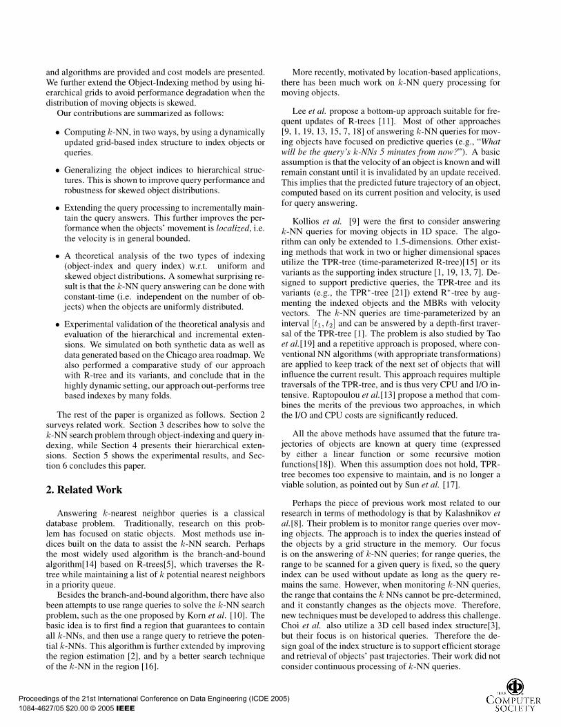
dicted by the analysis in Section 4. For R-tree-based ap-proaches, notice that the bottom-up update of the R-tree in-dex outperforms a complete rebuild of the R-tree index forrelatively small populations only. The reason is that in ourstudy, the average displacement of the moving objects is in-dependent of the population size. Therefore with larger pop-ulation, there is a greater degree of volatility which results inan increasing number of out-of-bounding-rectangle updatesby the bottom-up R-tree update algorithm.PERFORMANCE W.R.T. Nq Figure 19 shows the perfor-mance of the index structures with respect to increasingnumber of queries. Non-uniformity again makes the hierar-chical approach the best choice for large number of queries.

0 200 400 600 800 10000

1

2

3

4

5

6


Com

puta

tion

time

(sec

)

Performance of grid−based indices, Nq = 5,000

Query−IndexingOne−level Object−IndexingHierarchical Object−Indexing

(a) Grid-based approaches

0 20 40 60 80 1000

5

10

15

20

25

30

35

40

45


Com

puta

tion

time

(sec

)

Performance of R−tree−based indices, Nq = 5,000

R−tree overhaulR−tree bottom−up

(b) R-tree-based approaches

Figure 18. Performance of index structuresw.r.t NP

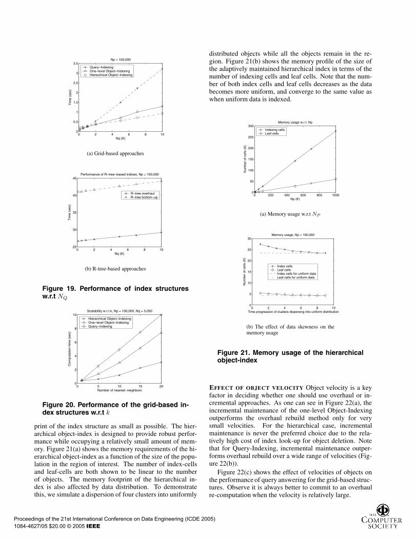
However, notice that Query-Indexing gives the best perfor-mance for small query workloads, which is expected sincein these cases, the query-index is easier to build, and asshown in Section 3.3, its query-answering cost is similarto that of Object-Indexing. With small workloads, the one-level Object-Indexing outperforms its hierarchical counter-part because it has a smaller index building overhead. But inthe case of larger query workloads, it is well worth the ex-tra effort to build a hierarchical object-index. Figure 19(b)shows the performance of the R-tree-based approaches. Thebottom-up update approach does not perform as well as theoverhaul rebuild approach, as it has greater index mainte-nance cost, as shown above, and query answering cost, dueto increased overlapping of the MBRs.SCALABILITY W.R.T. k The scalability of the proposedmethods with respect to k, the number of nearest neighbors,is also tested (on the skewed data set), and a typical resultis presented in Figure 20. All methods scale approximatelylinearly with respect to k, and again, the hierarchical Object-Indexing method shows best performance for all values ofk. The R-tree-based approaches are not shown in the graphbecause they are an order of magnitude slower than the grid-based methods.MEMORY USAGE Since all the data structures reside inmain memory, it is very important to keep the memory foot-


1084-4627/05 $20.00 © 2005 IEEE

0 2 4 6 8 100

0.5

1

1.5

2

2.5

3

3.5

Nq (K)

Tim

e (s

ec)

Np = 100,000

Query−IndexingOne−level Object−IndexingHierarchical Object−Indexing

(a) Grid-based approaches

0 2 4 6 8 1025

30

35

40

45

Nq (K)

Tim

e (s

ec)

Performance of R−tree−based indices, Np = 100,000

R−tree overhaulR−tree bottom−up

(b) R-tree-based approaches

Figure 19. Performance of index structuresw.r.t NQ

0 5 10 15 200

2

4

6

8

10

Number of nearest−neighbors

Com

puta

tion

time

(sec

)

Scalability w.r.t k, Np = 100,000, Nq = 5,000

Hierarchical Object−IndexingOne−level Object−IndexingQuery−Indexing

Figure 20. Performance of the grid-based in-dex structures w.r.t k

print of the index structure as small as possible. The hier-archical object-index is designed to provide robust perfor-mance while occupying a relatively small amount of mem-ory. Figure 21(a) shows the memory requirements of the hi-erarchical object-index as a function of the size of the popu-lation in the region of interest. The number of index-cellsand leaf-cells are both shown to be linear to the numberof objects. The memory footprint of the hierarchical in-dex is also affected by data distribution. To demonstratethis, we simulate a dispersion of four clusters into uniformly

distributed objects while all the objects remain in the re-gion. Figure 21(b) shows the memory profile of the size ofthe adaptively maintained hierarchical index in terms of thenumber of indexing cells and leaf cells. Note that the num-ber of both index cells and leaf cells decreases as the databecomes more uniform, and converge to the same value aswhen uniform data is indexed.

0 200 400 600 800 10000

50

100

150

200

250

300Memory usage w.r.t. Np

Np (K)

Num

ber

of c

ells

(K

)

Indexing cellsLeaf cells

(a) Memory usage w.r.t NP

0 2 4 6 8 100

5

10

15

20

25

30

Time progression of clusters dispersing into uniform distribution

Num

ber

of c

ells

(K

)

Memory usage, Np = 100,000

Index cellsLeaf cellsIndex cells for uniform dataLeaf cells for uniform data

(b) The effect of data skewness on thememory usage

Figure 21. Memory usage of the hierarchicalobject-index

EFFECT OF OBJECT VELOCITY Object velocity is a keyfactor in deciding whether one should use overhaul or in-cremental approaches. As one can see in Figure 22(a), theincremental maintenance of the one-level Object-Indexingoutperforms the overhaul rebuild method only for verysmall velocities. For the hierarchical case, incrementalmaintenance is never the preferred choice due to the rela-tively high cost of index look-up for object deletion. Notethat for Query-Indexing, incremental maintenance outper-forms overhaul rebuild over a wide range of velocities (Fig-ure 22(b)).

Figure 22(c) shows the effect of velocities of objects onthe performance of query answering for the grid-based struc-tures. Observe it is always better to commit to an overhaulre-computation when the velocity is relatively large.


1084-4627/05 $20.00 © 2005 IEEE

0 1 2 3 4 5

x 10−3

0

0.05

0.1

0.15

0.2

0.25

0.3

0.35

Velocity

Tim

e (s

ec)

Object−index maintenance

One−level rebuildingOne−level incremental updateHierarchical rebuildingHierarchical incremental update

(a) Object-index maintenance

0 0.01 0.02 0.03 0.04 0.050

0.5

1

1.5

2

2.5

3

3.5

4

4.5

Velocity

Tim

e (s

ec)

Query−index maintenance

Re−buildingIncremental update

(b) Query-index maintenance

0 0.005 0.01 0.015 0.02 0.0250

0.5

1

1.5

2

2.5

3

3.5

4

Velocity

Tim

e (s

ec)

Query answering

Object−Indexing (overhaul)Object−Indexing (incremental)Query−Indexing (incremental)Hierarchical Object−Indexing (overhaul)Hierarchical Object−Indexing (incremental)

(c) Query answering

Figure 22. The effect of velocity on index maintenance and query answering

6. Conclusion and Future Work

We have studied the problem of monitoring k-NN queriesover moving objects. We presented an analysis of two pro-posed approaches namely, query-indexing and object index-ing. We have validated the results of our analysis, presentedextensions of the basic methods to handle non-uniform dataefficiently and conducted a variety of experiments to explorethe benefits of our approach in a variety of parameter set-tings.

For future work, we would like to extend the (hierarchi-cal) Object-Indexing and Query-Indexing methods to han-dle other variations of k-NN queries, such as reverse k-NNqueries[1, 20], and group NN queries[12]. We are also con-sidering applying our algorithms in the context of spatialjoins of moving objects.

Acknowledgment We would like to thank A.O. Mendelzonand K.C. Sevcik for their valuable feedback.

References

[1] R. Benetis, C. Jensen, G. Karciauskas, and S. Saltenis. Near-est neighbor and reverse nearest neighbor queries for movingobjects. In IDEAS, 2002.

[2] S. Chaudhuri and L. Gravano. Evaluating top-k selectionqueries. In VLDB, 1999.

[3] W. Choi, B. Moon, and S. Lee. Adaptive cell-based index formoving objects. Data Knowl. Eng., 48(1), 2004.

[4] V. Gaede and O. Gunther. Multidimensional access methods.ACM Computing Surveys, 30(2):170–231, 1998.

[5] A. Guttman. R-trees: a dynamic index structure for spatialsearching. In SIGMOD Conference, 1984.

[6] M. Hadjieleftheriou. Spatial Index Library version 0.62b(C++ Version), 2003. University of California, Riverside.

[7] G. S. Iwerks, H. Samet, and K. Smith. Continuous k-nearestneighbor queries for continuously moving points with up-dates. In VLDB, 2003.

[8] D. V. Kalashnikov, S. Prabhakar, and S. E. Hambrusch. Mainmemory evaluation of monitoring queries over moving ob-jects. Distrib. Parallel Databases, 15(2):117–135, 2004.

[9] G. Kollios, D. Gunopulos, and V. J. Tsotras. Nearest neighborqueries in a mobile environment. In STDM, 1999.

[10] F. Korn, N. Sidiropoulos, C. Faloutsos, E. Siegel, and Z. Pro-topapas. Fast nearest neighbor search in medical imagedatabases. In VLDB, 1996.

[11] M. L. Lee, W. Hsu, C. S. Jensen, B. Cui, and K. L. Teo. Sup-porting frequent updates in r-trees: A bottom-up approach. InVLDB, 2003.

[12] D. Papadias, Q. Shen, Y. Tao, and K. Mouratidis. Group near-est neighbor queries. In ICDE, 2004.

[13] K. Raptopoulou, A. Papadopoulos, and Y. Manolopoulos.Fast nearest-neighbor query processing in moving-objectdatabases. GeoInformatica, 7(2):113–137, 2003.

[14] N. Roussopoulos, S. Kelley, and F. Vincent. Nearest neighborqueries. In SIGMOD Conference, 1995.

[15] S. Saltenis, C. S. Jensen, S. T. Leutenegger, and M. A. Lopez.Indexing the positions of continuously moving objects. InSIGMOD Conference, 2000.

[16] T. Seidl and H.-P. Kriegel. Optimal multi-step k-nearestneighbor search. In SIGMOD Conference, 1998.

[17] J. Sun, D. Papadias, Y. Tao, and B. Liu. Querying about thepast, the present and the future in spatio-temporal databases.In ICDE, 2004.

[18] Y. Tao, C. Faloutsos, D. Papadias, and B. Liu. Prediction andindexing of moving objects with unknown motion patterns.In SIGMOD Conference, 2004.

[19] Y. Tao and D. Papadias. Time-parameterized queries inspatio-temporal databases. In SIGMOD Conference, 2002.

[20] Y. Tao, D. Papadias, and X. Lian. Reverse knn search in ar-bitrary dimensionality. In VLDB, 2004.

[21] Y. Tao, D. Papadias, and J. Sun. The TPR*-Tree: An opti-mized spatio-temporal access method for predictive queries.In VLDB, 2003.

[22] K.-Y. Whang and R. Krishnamurthy. The Multilevel GridFile - a dynamic hierarchical multidimensional file structure.In DASFAA, 1991.


1084-4627/05 $20.00 © 2005 IEEE

monitoring k-nearest neighbor queries over moving objects · monitoring k-nearest neighbor queries...

Documents