MONETARY TRANSMISSION MECHANISM IN LITHUANIA

Igor Vetlov1

Bank of Lithuania Email: ivetlov@lb.lt

Vilnius 2003

1 All opinions expressed are those of the author and have not been endorsed by the Bank of Lithuania. I highly appreciate many valuable comments received from my colleagues: Raimondas Kuodis and Sigitas Šiaudinis, as well as Prof. David Mayes (Bank of Finland) and Iikka Korhonen (BOFIT). Any errors are the sole responsibility of the author.

Contents Abstract ............................................................................................................................... 3 1. Introduction..................................................................................................................... 4 2. Monetary Transmission Mechanism in Lithuania: Some Stylized Facts........................ 5 2.1. Monetary Policy Framework ....................................................................................... 5 2.2. Some Insights into the Operation of the CBA in Lithuania......................................... 8 2.3. Monetary Developments............................................................................................ 11 2.4. Financial Sector: Structure and Functioning.............................................................. 13 2.5. Real Sector and External Environment...................................................................... 17 3. Empirical Analysis of the MTM in Lithuania............................................................... 20 3.1. Identification of the Main Transmission Channels.................................................... 20 3.2. Model Specification and Estimation.......................................................................... 22 3.3. Impulse-Response Analysis of the Model ................................................................. 31 3.3.1. Short-term shock to the base rate............................................................................ 31 3.3.2. Medium-term shock to the base rate....................................................................... 33 3.3.3. Short-term shock to nominal exchange rate............................................................ 35 3.3.4. Medium-term shock to nominal exchange rate....................................................... 37 3.4. Shocks compared ...................................................................................................... 38 4. Conclusions and Future Research Agenda ................................................................... 40 References......................................................................................................................... 42 Appendix 1........................................................................................................................ 44 Appendix 2........................................................................................................................ 45 Appendix 3........................................................................................................................ 48

2

Abstract

This paper addresses the issues of the monetary transmission mechanism in Lithuania. First, we discuss the theoretical and empirical aspects of the monetary transmission mechanism in Lithuania in the light of the design of the monetary policy framework, development of the financial market, structure of the real sector and Lithuania’s dependence on an external environment. Second, we specify and estimate a small-scale structural macroeconomic model. The estimated model incorporates three traditional monetary transmission channels: interest rate, bank lending, and exchange rate channels. To study the strength of a particular monetary transmission channel we carry out impulse-response analysis of the estimated model and report the simulation results. Qualitatively the model’s response to the interest rate and exchange rate shocks is in agreement with economic intuition. Similar to the findings on the MTM in the euro area we find that investment demand in Lithuania is more sensitive than private consumption to the interest rate shock. In addition, the main burden of the economy’s adjustment to the shock is placed on the real variables as opposed to the nominal ones. Another finding is that the GDP response is greater and the CPI response is smaller under the interest rate shock scenario as compared to the exchange rate shock case.

Keywords: Monetary Transmission Mechanism, Currency board, EMU, Macroeconometric Models

JEL classification: C50, C52, E5

3

1. Introduction

The monetary transmission mechanism (MTM) represents a specific class of macroeconomic models that describe the channels through which monetary policy decisions are transmitted to the economy and affect policy objectives. The latter usually includes inflation, although unemployment and/or GDP growth can also be of some importance to monetary authorities. Among the main channels covered by the MTM are the interest rate channel, credit channel (bank-lending and balance sheet channels), exchange rate channel, and equity price channel (Mishkin, 1995). When conducting an empirical investigation of the MTM two broad stages can be identified. The first stage deals with transmission of monetary policy changes into changes in financial market conditions (money market interest rates, asset prices, the exchange rate etc.). The second one describes how changes in financial market conditions affect domestic GDP and inflation.

The relative significance of particular channels differs across the real world economies and largely depends on the underlying characteristics of the economy in question. For example, the exchange rate channel is usually more important for relatively small and open economies, while the interest rate channel is likely to be the key channel in a closed economy. The industrial structure of the domestic economy also has important implications for the MTM. Capital-intensive industries such as manufacturing and construction require relatively large investments; therefore, the larger the share of these industries in the economy the more important will be the interest rate channel. At the same time the level of development of the domestic financial market largely determines the strength of the MTM. The latter implies that understanding of the MTM requires evaluation of the depth and degree of sophistication of the domestic financial market as well as assessment of the significance of financial intermediation in financing the real sector.

Knowledge of the MTM underpins effective conduct of monetary policy. It allows not only selection of an adequate set of policy instruments but also their implementation in a timely way. An important issue here is stability of the MTM in the region. This is especially relevant when discussing the MTM in transition economies of Central and Eastern Europe (CEE). Given the enormous structural changes that the CEE economies experienced over the last decade it is reasonable to expect instability of the MTM. Thus, it is not surprising that at least at the start of the transition period many CEE economies have chosen not to exercise an active, independent monetary policy and instead have adopted a fixed exchange rate policy.

Lithuania (together with Estonia, Bulgaria, and more recently Bosnia-Herzegovina) represents an example of one end of the range of possible monetary policies, namely, a currency board arrangement (CBA). In general, the CBA can be characterized by three institutional features: (1) fixed exchange rate with respect to the anchor currency; (2) unrestricted convertibility and (3) backing of the monetary authorities’ liabilities in domestic currency by reserves of agreed foreign currency. On many occasions the CBA is implemented through passing a law. In practice one distinguishes between the orthodox CBA and the modern-day CBA. The orthodox or pure CBA requires full delegation of monetary policy to the currency board institution. The latter performs only technical activities, which ensure the required backing of the domestic liabilities. The currency board issues and redeems the domestic currency monetary liabilities on demand against

4

an ‘anchor’ currency at a predetermined exchange rate. While exhibiting all the main attributes of CBA, the modern-day CBA also retains some features of central banking (Ho (2002), Ghosh et al. (2000), Williamson (1995), and Bennett (1994)). The CBA adopted in Lithuania can be best characterized as a modern-day CBA. In the rest of the paper we use the term CBA to refer to the modern-day CBA.

A CBA significantly limits the ability of the monetary authorities to conduct discretionary monetary policy. The money stock becomes money demand determined. Possibilities for the monetary authorities to influence the domestic money stock are limited by coverage commitments and usually are confined to actions such as changing the reserve/liquidity requirements and playing the role of the lender-of-last-resort (to the extent allowed by the presence of excess foreign reserves).

The specifics of the monetary policy environment in Lithuania undoubtedly modify the usual MTM by augmenting the relative importance of particular transmitters. This paper aims at understanding the MTM in Lithuania. To do so we, first, discuss the theoretical and empirical aspects of the monetary transmission mechanism in Lithuania in the light of the design of monetary policy framework, development of the financial market, structure of the real sector and Lithuania’s dependence on the external environment. Next, we specify and estimate a small-scale structural macroeconomic model for the Lithuanian economy. To study the strength of a particular monetary transmission channel we carry out impulse-response analysis of the estimated model and report the simulation results. Finally, we conclude and set agenda for future research.

In broader terms the paper contributes to the more general discussion of monetary transmission mechanisms in the euro area and EU accession countries. Noting that the knowledge of monetary transmission mechanisms helps to answer many questions regarding countries’ participation in a currency union in the light of the optimal currency area considerations, we hope that the paper will also add to an economic debate on Lithuania’s future participation in the EMU.

2. Monetary Transmission Mechanism in Lithuania: Some Stylised Facts

2.1. Monetary Policy Framework

The modern history of Lithuanian central banking began with the re-establishment2 of the Bank of Lithuania (BoL) in February 1990. While remaining a part of the rouble zone Lithuania had practically no room for independent monetary policy. Monetary conditions were theoretically in the hands of the monetary authority in Moscow but were heavily influenced by the unstable economic situation both in Lithuania and the rest of the USSR.

The main stages of price liberalization in Lithuania took place in 1991–1992 and in the face of monetary overhang led to a dramatic increase in domestic inflation: from 9.1 per cent in 1990 to 216.4 and 1020.5 per cent in 1991 and 1992, respectively. At the same time the domestic currency depreciated heavily. Other unfavourable developments which fuelled domestic price increase in the first years of Lithuania’s economic transition were

2 The Bank of Lithuania was first established in Kaunas in 1922. Under Soviet occupation (1940–1990) it did not exist.

5

the economic blockade3 imposed by the Soviet Union, adverse supply shocks stemming from the liberalization of prices on energy and raw materials imported from Russia, and the inflationary fiscal policy of the Lithuanian Government4.

Seeking to stabilize domestic inflation the BoL embarked on currency reforms that gradually led to the introduction of today’s national currency, the litas, on June 25, 1993. The subsequent tight monetary policy brought a significant deceleration in inflation down to 410.2 per cent in 1993. From its introduction the litas appreciated, signalling that the initial litas exchange rate was considerably undervalued. The BoL’s interventions in the foreign exchange market stabilized the litas exchange rate by the end of 1993.

In the course of 1992–1993 the BoL applied a wide range of monetary policy instruments to combat inflation: minimum reserve requirements, credit ceilings, deposit and credit auctions (Bank of Lithuania, 1995). The BoL specifically targeted net domestic assets (1992 October-December) and the monetary base (1993). Development of the domestic foreign exchange market for the litas allowed the BoL to gain an additional instrument in curbing domestic inflation. Given the smallness and openness of the Lithuanian economy the stable exchange rate of the domestic currency was regarded as akin to price stability. At the same time, the ongoing economic recession, high degree of dollarization of domestic economy5, and a loose fiscal policy created uncertainty about the external stability of the litas. On the other hand, the BoL’s policy lacked credibility and transparency needed to accelerate further decreases in inflation and interest rates. These considerations led to the adoption of the currency board arrangement (CBA) from the 1st of April 1994. Its legal basis was the Law on the Credibility of the Litas (passed in March 1994). The law guaranteed at least 100 per cent coverage of litas in circulation by gold and foreign exchange reserves of the BoL. In compliance with the law the exchange rate of the litas was ultimately fixed to the anchor currency, the US dollar (at a rate 4 litas for 1 US dollar). It could only be changed by joint agreement between the Lithuanian Government and the BoL under the circumstances when the stability of the entire economy was endangered. Ever since then the Lithuanian economy has operated under the CBA. Over the CBA period domestic inflation fell gradually and since 1997 it has remained at single digit levels.

Following the economic recovery and difficulties in the domestic banking sector in 1995–1996, ideas regarding dismantling the CBA began to spread among Lithuanian policymakers. It was hoped that a move to a more independent monetary policy would permit the use of a larger spectrum of policy instruments enabling the BoL to fine-tune domestic economy. Thus, on January 16, 1997 a three-stage programme for 1997–1999 aimed at gradual dismantling of the CBA was approved and the BoL began to develop an active monetary policy. However, the Southeast Asian crisis in 1997 and the financial crisis in Russia in 1998 generated fears of default on government obligations as well as expectations of devaluation. In this new environment the idea of the dismantling the CBA was given up and Lithuania returned to the terms of the IMF Memorandum (early 2000), which obliged Lithuania to preserve the CBA and to tighten fiscal policy. 3 The blockade cut off supplies and trade flows, hampering the work of the railways, the port, banks, the payments system, as well as restricting international communications. It was imposed on 16 April 1990 and continued until the failure of the coup in Moscow in August 1991. 4 From January 1991 until September 1992 the BoL issued significant credits to the Government. In this period the volume of all credits granted by the BoL rose 12.1 times to 24 bn roubles, almost half of which was used to finance the government budget (Bank of Lithuania, 1995). 5 See Vetlov (2001).

6

In 1999 ‘Guidelines for the application of Bank of Lithuania monetary policy instruments’ was published (Bank of Lithuania, 1999a). The ‘Guidelines’ were intended as a practical document clarifying the framework of the policy conducted by the BoL. It reflected the evolution of the BoL’s view regarding monetary policy. On the one hand, it was clear that the CBA would remain in place at least in the short and medium run. On the other hand, it was still thought useful to apply active monetary policy instruments under the CBA. Similar to the Law on the Central Bank (1994) the ‘Guidelines’ defined the main objective of the BoL as seeking the stability of the currency of the Republic of Lithuania. Other objectives of the BoL included promotion of the development of domestic financial market and the acceleration of Lithuania’s integration into the EU. The latter was mainly to be implemented through harmonization of monetary policy instruments with European Central Bank (ECB) requirements.

To meet the above-mentioned objectives the BoL applied a range of monetary policy instruments. These included reserve requirements, lending facilities (overnight loans and liquidity loans), and open market operations (repo auctions and time deposit auctions). The reserve requirement was applied at a rate of 10 per cent and proved to be the most effective policy instrument available to the BoL. Declining systemic risk in the domestic banking sector combined with the aim of bringing BoL monetary policy instruments in line with the ECB led to a reduction in the reserve requirement from 10 to 8 per cent in October 2000 and further to 6 per cent in May 2002. The BoL intends to reduce the reserve requirement further, however, the subsequent decrease of the reserve requirement will depend on the general stability of macroeconomy and the banking system.

Open market operations (OMOs) were applied during the three-stage programme for 1997–1999 as a minor fine-tuning instrument under the conditions of the CBA and structural liquidity surplus of the banking system (two particular systemic liquidity shocks were due to the saving restitution programme which aimed at recovering the savings lost during the high inflation in 1991–19936 and Y2K related adjustments). The OMOs were specifically aimed at levelling off temporary banking system liquidity fluctuations and helping the domestic banking system to adjust to developments in international financial markets. The need for such market operations, however, has quickly diminished because commercial banks have established close ties with international markets abroad, thereby enabling them to manage their liquidity more effectively. Additionally, in practice, the timing, magnitude and, especially, optimal level of interest rates were usually not very clear. On the other hand, discretionary interventions by the BoL could also raise market expectations about intentions of control of its interest rates. Thus, the last repo auction by the BoL was conducted in October 1998 and the last time deposit auction was held in February 2000 (Bank of Lithuania 2001, 2000).

In the second half of the 1990s, especially after the Russian financial crisis in 1998, the intensity of economic relations between Lithuania and the EU substantially increased and large swings in the euro-dollar exchange rate became rather costly for the Lithuanian economy. In addition, maintenance of the peg versus the US dollar seemed inconsistent

6 The programme was funded from the proceeds of the Lithuanian Telecommunication company privatisation. These proceeds were initially held at the BoL. At the end of 1998 the Ministry of Finance started transferring the funds from the BoL into the residents’ bank accounts. The rise in bank deposits brought a substantial increase in excess reserves in the banking sector. Later, however, the newly created deposits were gradually converted into foreign currency deposits. This allowed the Lithuanian banks to invest the excess reserves abroad balancing the currency composition of the banks’ liabilities and assets.

7

with the Lithuanian long run strategy of integration into the EMU. Thus, after consultation with the IMF and the Lithuanian Government, on the 2nd of February 2002 the BoL re-pegged the Lithuanian litas to the euro at its ongoing market rate. Earlier announcements of the BoL hint that the CBA will be maintained until full Lithuanian membership in the EMU. Thus, the BoL has gradually returned to a passive monetary policy approach, which is what one would actually expect under a CBA regime. It also implies that the policy framework defined in the “Guidelines” can now be used to characterize the current operations of the BoL only with reservations.

Finally, the new law on the BoL came into force in March 2001. It underlined the independence of the central bank with respect to the Government and significantly altered the terms of reference of policy-making at the BoL. The new law explicitly defined seeking price stability as the overriding objective of the BoL and this objective is to be implemented within the current CBA framework indirectly: through a fixed exchange rate, automatic money market adjustment, and low inflation expectations.

2.2. Some Insights into the Operation of the CBA in Lithuania

As in case of a fixed exchange rate and liberal capital regime, under a CBA monetary policy is limited in achieving macroeconomic objectives, and the main burden of demand management falls on the shoulders of fiscal policy. Money supply is no longer within control of the monetary authorities and becomes an endogenous variable of the system. Instead, money demand plays the key role in the determination of the domestic money stock. Shocks to money demand will fully translate into changes in the money stock via adjustment in the BOP position.

To fix the idea in what follows we shall use a small open-economy model of monetary policy under a fixed exchange rate, called the monetary approach to the balance of payments. The model was developed by the IMF in the 1950-60s, and has proved useful in evaluating macroeconomic policies of countries with characteristics similar to those of today’s Lithuania.

Because of its concentration on the money market, the monetary approach to the balance of payments involves an explicit specification of the money supply and money demand function. The supply of money (Ms

t) is the product of the stock of high-powered money (Ht) and the money supply multiplier (mt). The latter reflects the behaviour of asset-holders and the banking system:

Mst=mt·Ht [i]

By definition, the stock of high-powered money (the liabilities of the monetary authorities) is equal to the domestic currency value of the stock of foreign reserves, E•Rt (where E is the fixed exchange rate, defined in European terms, and Rt is the foreign currency value of foreign reserves), and the net domestic asset holdings of the monetary authorities (Dt) (also adjusted for the capital of the monetary authorities):

Ht=Et·Rt+Dt [ii]

Under the CBA, as opposed to the usual fixed exchange rate regime, only foreign reserves can cover the high-powered money so that given, for instance, at least a 100 percent coverage requirement the following constraint must hold: Ht≤E·Rt. The latter

8

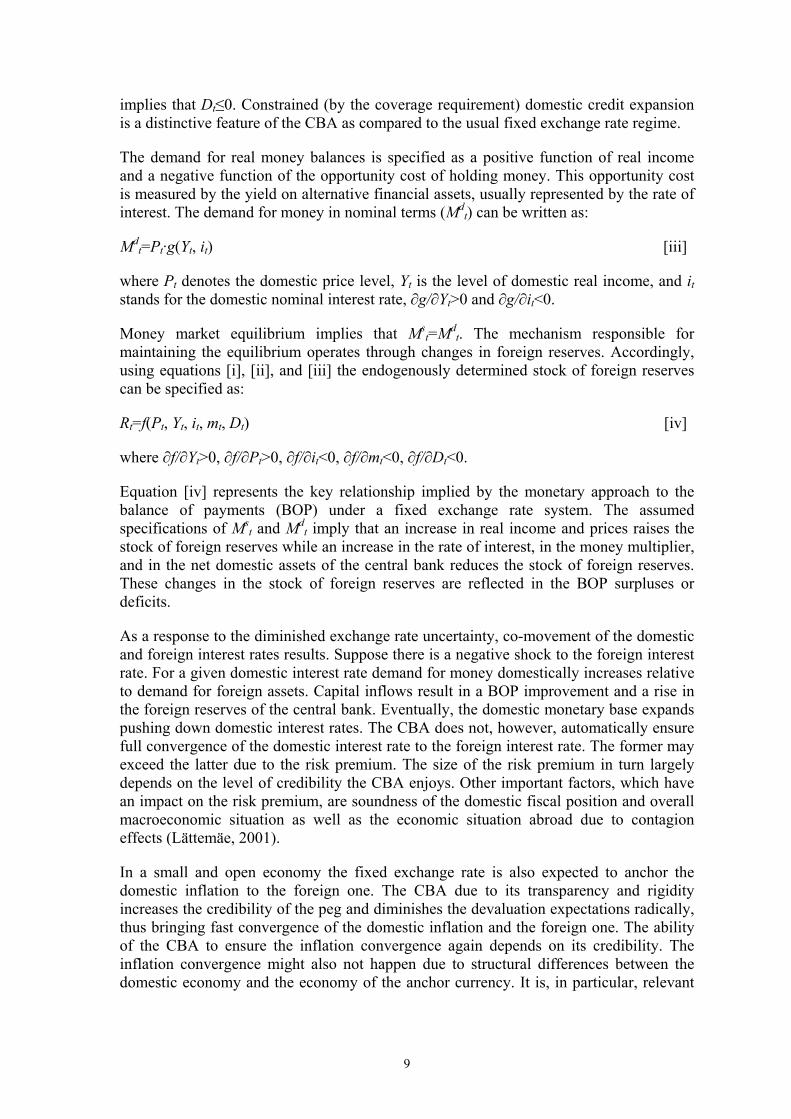
implies that Dt≤0. Constrained (by the coverage requirement) domestic credit expansion is a distinctive feature of the CBA as compared to the usual fixed exchange rate regime.

The demand for real money balances is specified as a positive function of real income and a negative function of the opportunity cost of holding money. This opportunity cost is measured by the yield on alternative financial assets, usually represented by the rate of interest. The demand for money in nominal terms (Md

t) can be written as:

Mdt=Pt·g(Yt, it) [iii]

where Pt denotes the domestic price level, Yt is the level of domestic real income, and it stands for the domestic nominal interest rate, ∂g/∂Yt>0 and ∂g/∂it<0.

Money market equilibrium implies that Mst=Md

t. The mechanism responsible for maintaining the equilibrium operates through changes in foreign reserves. Accordingly, using equations [i], [ii], and [iii] the endogenously determined stock of foreign reserves can be specified as:

Rt=f(Pt, Yt, it, mt, Dt) [iv]

where ∂f/∂Yt>0, ∂f/∂Pt>0, ∂f/∂it<0, ∂f/∂mt<0, ∂f/∂Dt<0.

Equation [iv] represents the key relationship implied by the monetary approach to the balance of payments (BOP) under a fixed exchange rate system. The assumed specifications of Ms

t and Mdt imply that an increase in real income and prices raises the

stock of foreign reserves while an increase in the rate of interest, in the money multiplier, and in the net domestic assets of the central bank reduces the stock of foreign reserves. These changes in the stock of foreign reserves are reflected in the BOP surpluses or deficits.

As a response to the diminished exchange rate uncertainty, co-movement of the domestic and foreign interest rates results. Suppose there is a negative shock to the foreign interest rate. For a given domestic interest rate demand for money domestically increases relative to demand for foreign assets. Capital inflows result in a BOP improvement and a rise in the foreign reserves of the central bank. Eventually, the domestic monetary base expands pushing down domestic interest rates. The CBA does not, however, automatically ensure full convergence of the domestic interest rate to the foreign interest rate. The former may exceed the latter due to the risk premium. The size of the risk premium in turn largely depends on the level of credibility the CBA enjoys. Other important factors, which have an impact on the risk premium, are soundness of the domestic fiscal position and overall macroeconomic situation as well as the economic situation abroad due to contagion effects (Lättemäe, 2001).

In a small and open economy the fixed exchange rate is also expected to anchor the domestic inflation to the foreign one. The CBA due to its transparency and rigidity increases the credibility of the peg and diminishes the devaluation expectations radically, thus bringing fast convergence of the domestic inflation and the foreign one. The ability of the CBA to ensure the inflation convergence again depends on its credibility. The inflation convergence might also not happen due to structural differences between the domestic economy and the economy of the anchor currency. It is, in particular, relevant

9

to transition economies like Lithuania experiencing relatively high productivity gains (the Balassa-Samuelson effect).

Lastly, one of the important implications of the CBA cited in the related economic literature is described as the automatic money supply mechanism. The idea behind it is usually illustrated by a textbook example where the BOP surpluses/deficits are automatically adjusted via domestic liquidity loosening/tightening induced by changes in the foreign reserves of the monetary authorities. This view presumes a tight (practically one-to-one) relationship between the foreign reserves and monetary base. In other words, there is no room for policy discretion whatsoever. In real world CBA, however, deviation from the “iron clad rule” is possible. A particular case, which is especially relevant to the Lithuanian experience, is when the Government holds its deposits with the central bank. These deposits reflect the Ministry of Finance’s treasury operations around the fiscal year: tax collection, privatisation receipts, money from the Eurobond issues, various public expenditures etc.

In Lithuania, Government deposits with the BoL earn no interest if held in domestic currency and the base currency interest if held in foreign currency. Therefore, it is not surprising that almost all of the Government’s deposits with the BoL are denominated in foreign currency. Since Government deposits in foreign currency are included in the BoL’s official foreign reserves, changes in the former lead to changes in the latter. Thus, in the case of Lithuania, increases or reductions in Government deposits with the BoL constitute a potential source of disturbances to the domestic money market. Whether the money stock in the economy is altered depends ultimately on money demand behaviour. Injection of the litas into the economy by using the deposits produces imbalance in the money market. For given money demand a reduction in the foreign reserves will clear the market.

Figure 1. Foreign reserves and domestic liabilities of the Bank of Lithuania, billions of litas, 1997–2002

1

2

3

4

5

6

7

8

9

1997 1998 1999 2000 2001 2002 2003

Foreign reserves Central government deposits Monetary base

Source: Bank of Lithuania

Indeed, as follows from Figure 1, since 1998 about 90 per cent of the variation in the official foreign reserves in Lithuania is explained by discrete actions of the Ministry of Finance executed via treasury operations, which are reflected in the Treasury’s account with the BoL. Foreign reserves increase when the Government puts privatisation receipts or money from the Eurobond issues. When the money is converted into litas and injected to the banking system as payment for goods, labour services or as savings restitution, the

10

consequent disequilibrium in the money market is rapidly cleared through the foreign exchange window.

2.3. Monetary Developments

The CBA framework undoubtedly affects the development of the key monetary indicators in Lithuania. Figure 2 shows that the monetary base coverage requirement has been maintained rigorously. In fact foreign reserves of the BoL significantly exceeded the monetary base. It is noteworthy that over the whole period the foreign reserves of the BoL were also closely matching narrow money aggregate M1. Overall, the dynamics of the main monetary aggregates resembles that of the foreign reserves of the BoL revealing the CBA monetary policy rule at work. Short-term differences in dynamics of the narrow monetary aggregates and foreign reserves observed since 1998, as discussed above, should be primarily attributed to the shocks to the Government’s deposits held with the BoL.

Visually, the development of the broad money aggregate M2 seems to diverge from that of the foreign reserves of the BoL and other monetary aggregates. However, this is mainly due to the inclusion of foreign currency deposits in M2. As indicted in Table 1 foreign currency deposits constitute a large part of M2 and, thus, substantially distort the relationship between M2 and the foreign reserves of the BoL. Once foreign currency deposits are subtracted from M2 one finds that broad money follows the foreign reserves of the BoL similarly as narrow money, which is denominated in litas only (see Table 1 in Appendix 1 for cross correlation analysis of the data in levels and growth rates of different frequencies).

Figure 2. Main monetary aggregates in Lithuania, billions of litas, 1993–2003

123456789

101112131415

1993 1994 1995 1996 1997 1998 1999 2000 2001 2002 2003

M2 M1 Foreign reserves M0

Source: Bank of Lithuania

The dynamics of money aggregates in Lithuania was affected by macroeconomic stabilization and development of the domestic financial sector. As shown in Table 1 money stock growth had largely declined by the end of the last decade. Two rapid decelerations in the indicators were recorded in 1996 and 1999. The first was due to the domestic banking crisis while the second one reflected the economic decline in Lithuania. The acceleration of money stock growth observed over 2000–2002 should be primarily attributed to domestic economic recovery, progress in banking sector privatisation, as well as reduction in reserve requirements in 2000 and 2002. Despite the recent increase in

11

the growth rate of money stock, the GDP monetization ratio remains very low in Lithuania even by Central and Eastern European (CEE) standards. The roots of this can be traced in slow domestic financial sector development (see also section 2.4 for more details).

Table 1. Main monetary indicators in Lithuania, end of the period, % 1993 1994 1995 1996 1997 1998 1999 2000 2001 2002 M0 growth 170 61.9 34.6 2.1 32.0 29.6 -9.3 2.3 8.2 13.4 M1 growth 153 41.7 40.9 3.5 41.5 9.0 -5.3 7.5 18.9 27.4 M2 growth 100 63.0 28.9 -3.5 34.1 14.5 7.7 16.5 21.4 19.3 M2-to-GDP 23.1 25.8 23.3 17.2 19.0 19.4 21.0 23.2 26.5 29.3 Foreign currency deposits-to-M2 25.5 26.8 26.0 24.4 21.2 24.1 30.4 34.0 32.9 30.8 Bilateral rate vs. the USD† -23.8 -2.2 0.0 0.0 0.0 0.0 0.0 0.0 0.0 15.1 Bilateral rate vs. the DEM/EUR† n.a. -11.1 -9.2 7.1 12.7 -6.5 13.6 11.6 0.2 3.4 Nominal effective exchange rate† n.a. 95.9 13.4 11.1 16.8 49.5 23.2 10.1 2.4 11.0 Real effective exchange rate† n.a. 20.8 -4.5 10.0 15.4 21.9 6.4 2.3 -2.2 4.0

Sources: Bank of Lithuania, Lithuanian Department of Statistics, and authors’ calculations. Note: †– negative sign reflects depreciation of the domestic currency.

Figure 3. The litas real effective rates with respect to the European Union (REER_EU), the Commonwealth of Independent States (REER_CIS), and Central and Eastern European countries (REER_CEE), and overall real exchange rate (REER), 1994 April=100, exchange rate is defined in American terms

80

100

120

140

160

180

200

220

240

260

1994 1995 1996 1997 1998 1999 2000 2001 2002 2003

REER REER_EUREER_CEE REER_CIS

Source: Bank of Lithuania

Although pegged to the US dollar, the litas has largely fluctuated against the currencies of Lithuania’s major foreign trade partners in the EU, CEE, and the CIS in 1994–2001 (see Table 1). In particular, a large nominal appreciation of the litas was recorded against the German mark in 1996–1997 and the euro in 1999–2000. In addition, since its introduction the litas has been strengthening against the currencies of the CIS countries. The nominal effective (i.e. weighted by trade shares) exchange rate reveals high litas appreciation rates throughout the period considered.

The large devaluation of the CIS currencies was usually coupled with excessive inflation in these countries. Therefore, unless the nominal effective exchange rate of the litas is corrected for inflation differences, the indicator is useless when judging the real value of the litas. The last row in Table 1 shows the rate of Consumer Price Index based real

12

effective exchange rate of the Lithuanian litas7. Still, except for 1995 and 2001, the litas appreciated significantly. In the period from 1994 to 1996 high inflation in Lithuania was the driving force behind the real appreciation of the litas. Later, as domestic inflation declined to EU levels, it was the weakening euro that was responsible for further real appreciation of the litas. More detailed breakdown of the litas real effective exchange rate in Figure 3 reveals the largest real appreciation against the EU currencies and the smallest one in case of the CEE countries. The litas real value against the CIS currencies is found to be the most volatile one with the sharpest appreciation recorded in the second half of 1998 following the Russian rouble devaluation.

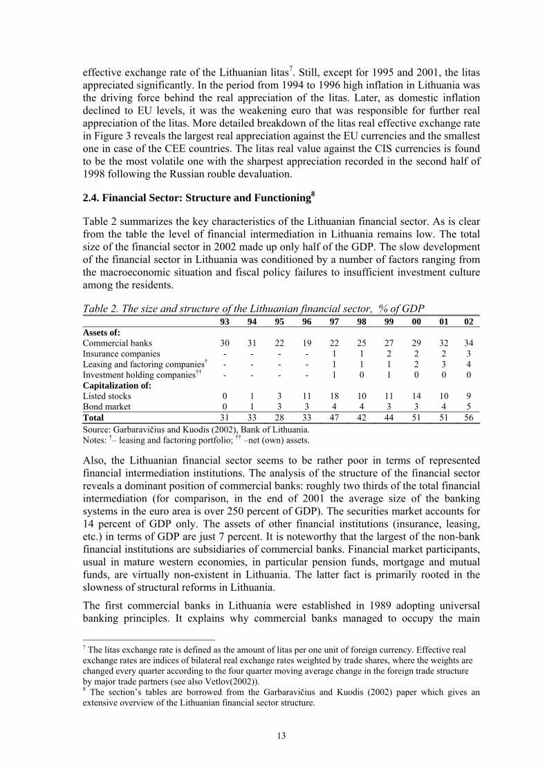
2.4. Financial Sector: Structure and Functioning8

Table 2 summarizes the key characteristics of the Lithuanian financial sector. As is clear from the table the level of financial intermediation in Lithuania remains low. The total size of the financial sector in 2002 made up only half of the GDP. The slow development of the financial sector in Lithuania was conditioned by a number of factors ranging from the macroeconomic situation and fiscal policy failures to insufficient investment culture among the residents.

Table 2. The size and structure of the Lithuanian financial sector, % of GDP 93 94 95 96 97 98 99 00 01 02

Assets of: Commercial banks 30 31 22 19 22 25 27 29 32 34 Insurance companies - - - - 1 1 2 2 2 3 Leasing and factoring companies† - - - - 1 1 1 2 3 4 Investment holding companies†† - - - - 1 0 1 0 0 0 Capitalization of: Listed stocks 0 1 3 11 18 10 11 14 10 9 Bond market 0 1 3 3 4 4 3 3 4 5 Total 31 33 28 33 47 42 44 51 51 56 Source: Garbaravičius and Kuodis (2002), Bank of Lithuania. Notes: †– leasing and factoring portfolio; †† –net (own) assets. Also, the Lithuanian financial sector seems to be rather poor in terms of represented financial intermediation institutions. The analysis of the structure of the financial sector reveals a dominant position of commercial banks: roughly two thirds of the total financial intermediation (for comparison, in the end of 2001 the average size of the banking systems in the euro area is over 250 percent of GDP). The securities market accounts for 14 percent of GDP only. The assets of other financial institutions (insurance, leasing, etc.) in terms of GDP are just 7 percent. It is noteworthy that the largest of the non-bank financial institutions are subsidiaries of commercial banks. Financial market participants, usual in mature western economies, in particular pension funds, mortgage and mutual funds, are virtually non-existent in Lithuania. The latter fact is primarily rooted in the slowness of structural reforms in Lithuania.

The first commercial banks in Lithuania were established in 1989 adopting universal banking principles. It explains why commercial banks managed to occupy the main

7 The litas exchange rate is defined as the amount of litas per one unit of foreign currency. Effective real exchange rates are indices of bilateral real exchange rates weighted by trade shares, where the weights are changed every quarter according to the four quarter moving average change in the foreign trade structure by major trade partners (see also Vetlov(2002)). 8 The section’s tables are borrowed from the Garbaravičius and Kuodis (2002) paper which gives an extensive overview of the Lithuanian financial sector structure.

13

niches of financial intermediation already in the first years of transition. Nevertheless, the development of the banking sector was not easy. Over the last decade the banking sector went though the period of “mushrooming”9, banking crisis and a period of consolidation. Important factors affecting the development of the sector were privatisation, opening up the market to foreign competition and building up institutional credibility. Today there are 14 commercial banks (of which 4 are foreign bank branches) in Lithuania. All the banks are privately owned. Non-residents (mostly Scandinavians and Germans) control 12 banks, which account for about 98 percent of banking assets. Another feature of the Lithuanian banking sector is a high level of concentration. At the end of 2002 the top 3 banks constituted 78 percent (74 percent in 2002) of total banking assets while the biggest bank in terms of assets occupied 40 per cent of the market.

Table 3. The stock of credit in Lithuania, % of GDP 1993 1994 1995 1996 1997 1998 1999 2000 2001 Domestic credit and net foreign assets of domestic banks

Credit to private sector 13.9 17.7 15.4 10.9 10.0 10.5 11.7 10.8 13.1 Corporate sector 12.3 15.5 13.7 9.6 8.4 8.2 9.1 8.4 9.9 Households 1.6 1.6 1.0 0.8 1.0 1.2 1.6 1.3 1.5 NBFI† 0.0 0.1 0.2 0.1 0.4 1.0 1.0 1.1 1.6 Net credit to public sector†† -7.3 -5.2 -4.7 -2.2 0.0 1.1 1.4 3.1 4.8 Credit to public sector 3.5 3.8 3.1 3.2 5.3 5.4 4.9 5.9 6.6 Liabilities to public sector 10.8 9.0 7.8 5.4 5.3 4.3 3.5 2.9 1.8 Net foreign assets 2.3 0.3 0.5 1.2 0.8 -1.1 -0.7 1.7 1.3 Foreign assets 2.6 2.3 2.0 3.6 3.7 2.7 3.9 6.1 6.3 Foreign liabilities 0.3 2.0 1.5 2.4 2.9 3.8 4.6 4.5 5.0 Foreign credit to private non-banks†††

Loans - - - 5.3 7.2 7.9 7.8 7.9 6.9 Bonds - - - 0.0 1.6 0.5 0.2 0.2 0.8

Source: Garbaravičius and Kuodis (2002). Notes: †– non-bank financial institutions; †† – public sector does not include monetary authorities; ††† – foreign credit includes cross-border loans and bonds held by foreign investors, but excludes trade credit and inter-company loans by foreign (parent) company.

The analysis of the balance sheet structure of the banking sector reveals that the domestic credit to the private sector remains very low (see Table 3). In 2001 it made up only 13 per cent of GDP. The lion’s share of credit was directed to the corporate sector while households received only 1.5 percent of GDP. The growth in private credit has been restrained by poor investment opportunities and financial turbulence, in particular, the domestic banking crisis in the mid-1990s10 and the Russian financial crisis in 1998. Instead a tendency has been observed to channel more financial resources towards the public sector and foreign assets.

On the liabilities side, household deposits constitute the main source of funding of the banking sector. Although the level of savings-to-GDP ratio in Lithuania is comparable to the euro zone economies, the share of bank deposits in GDP is much lower in Lithuania. The main reason for the saving-deposit wedge in Lithuania is low confidence in the banking system. Given poor development of other segments of the domestic financial sector a substantial share of savings was embodied in the form of cash holdings, in particular, foreign currency banknotes. 9 The number of commercial banks increased from 8 in 1990 to 27 in 1993. 10 Business defaults, poor bank supervision, and illegal (connected lending) activities by domestic banks led to the bank crisis at the end of 1995 – beginning of 1996. It constituted a considerable blow to the credibility of the banking sector. As a result, bank assets as a percentage of GDP shrank from 31 percent in 1994 to 19 percent in 1996. It took five years to reach the pre-crisis level.

14

The currency composition of bank deposits shows a high degree of asset dollarization: foreign currency deposits made up roughly one third of total deposits. It is noteworthy that the US dollar denominated deposits dominate in the group of foreign currency deposits, which is consistent with the eight-year peg to the US dollar. However, following the litas re-peg to the euro the share of dollar denominated deposits began to decline.

The securities market in Lithuania began to function in 1993 with the opening of the National Stock Exchange of Lithuania (NSEL). The capitalization of the securities market was growing steadily and in 1997 reached 22 percent of GDP. Important factors behind the growing securities market were the opening of the Government securities market in 1994 and the launch of cash-based privatisation in 1995. Despite some progress in developing a domestic securities market the overall liquidity of the NSEL has been rather low. The total NSEL turnover in 2001 was only 460 million USD of which more than half was due to the Government securities market turnover.11 At the same time, the corporate debt market remains negligible. Overall, among the potential factors hindering development of the securities markets in Lithuania are the small size of the domestic market, lack of institutional investors (pension funds, mutual funds etc.), prohibition of issuing debt securities denominated in foreign currencies domestically and a poor investment culture. For the above reasons the Lithuanian securities market provides only limited financial resources for the private sector. For example, the value of private equity issues was just 0.5 and 1 percent of GDP in 2000 and 2001, respectively.

The low level of financial intermediation in Lithuania can also be traced by looking at the structure of the domestic corporate investment sources. The latter reveals that the internal resources remain the dominant source of corporate investment. Despite some increase in corporate borrowing in 2001 external sources still financed only 30 per cent of gross fixed capital investment.

Table 4. External corporate funding in Lithuania, % of gross fixed capital investment 1997 1998 1999 2000 2001 Domestic sources 11.3 12.8 13.4 4.0 20.0

Bank credit 1.8 2.9 3.8 -1.0 10.5 Equity issues 9.4 8.1 10.0 2.6 5.0 Leasing - 1.8 -0.4 2.4 4.5

Foreign sources 31.9 5.1 1.6 10.5 9.5 Inter-company loans 3.9 4.2 1.1 4.5 3.1 Loans 11.6 6.2 -0.8 2.7 -2.6 Bond issues 6.4 -3.7 -1.3 0.0 3.3 Trade credit 9.3 -0.9 1.9 1.9 5.6 Other liabilities 0.6 -0.7 0.7 1.3 0.2

Source: Garbaravičius and Kuodis(2002).

Several explanations of the importance of internal financing relative to the external one can be distinguished. On the one hand, up until the end of 2001 the reinvested corporate profits were tax deductible making internal financing rather attractive. On the other hand, relatively high interest rates and complex requirements for domestic bank credit made bank borrowing costly or even inaccessible. At the same time poor knowledge among Lithuanians about borrowing opportunities abroad coupled with the fact that the

11 Indeed, Lithuania has a relatively well-developed market for the Government securities. The latter resulted from the need to finance substantial government budget deficits recorded throughout the last decade.

15

Lithuanian companies had to establish credibility abroad from scratch worked as a major stumbling block on the way to foreign credit.

From the analysis above at least three basic observations follow. First, the financial sector in Lithuania remains underdeveloped (narrow and thin). Second, market performance is determined mainly by actions undertaken by commercial banks and the Government. The last, though by no mean the least important, observation is that the Lithuanian financial market becomes increasingly integrated into the international financial system, which implies larger Lithuania’s financial sector dependence on the latter. All three observations have certain implications for the MTM in Lithuania. On the one hand, an underdeveloped domestic financial market largely undermines the interest rate and lending channels. There is also little evidence supporting the importance of the balance sheet and equity channels. On the other hand, the commercial bank retail interest rate, interest rates paid on Government securities and foreign money market interest rate are likely to be the key interest rates to be considered when modelling the Lithuanian MTM.

Figure 4. The Lithuanian Government’s Treasury bill rate of 3-12 month maturity, three-months Vilnius (LTL) and London (USD) inter-bank offer interest rates

0

5

10

40

35

25

20

15

30

1995 1996 1997 1998 1999 2000 2001 2002 2003

3 months LTL IBOR3 months USD IBOR

Tbills rate

ource: Bank of Lithuania, BloombergS

Figure 4 depicts developments in the three-month Vilnius12 and London USD inter-bank offer rates (LTL IBOR and USD IBOR, respectively), and the Lithuanian T-bill interest rates. Up until 1998 the large difference between Lithuanian interest rates and LIBOR was associated both with the risk premium (currency and systemic) and excessive domestic inflation. As inflation moderated in Lithuania, however, the observed spreads in 1998–1999 should be largely attributed to the risk premium. Indeed, the comparison of the available data for the LTL IBOR and USD IBOR yields a large positive spread in 1999, which was a direct result of economic and political uncertainty (including the risk of devaluation) in the aftermath of the Russian crisis. The spread reached a peak in autumn 1999 following the change of the Lithuanian Government in October and rumors about default on the Government financial obligations as well as devaluation fears.

From the beginning of 2000 the spread significantly declined as the new Government tightened fiscal policy13 and convinced the public of its intention of maintaining the

12 Vilnius inter-bank rates were not compiled until 1997 September. 13 The number of new T-bill auctions has declined considerably since the beginning of 2000.

16

CBA. In addition, the significant improvements in direct relations between domestic and foreign banks since the beginning of 2000 have also contributed to the decline in the spread between the LTL IBOR and the USD IBOR.

Analysis of bank deposit and loan interest rates14 in Lithuania over the period from 1995 to 2002 suggests that the basic developments of the foreign money market were transmitted to the domestic bank interest rates once the level of inflation in Lithuania declined to levels comparable to those in western economies. It is noteworthy that the spread between loan and deposit rates remains relatively large indicating inefficiencies in the Lithuanian banking sector, high credit risk, relatively high reserve requirements, and large payments by banks to the Deposit Insurance Fund15. The low level of competition among domestic banks (as indicated by high concentration) is a further factor in the large spread.

Figure 5. Three-month USD and DEM inter-bank offer, 1-3 month bank time deposit in litas, and up to 3 months bank litas loan interest rates, %

5

0

10

15

20

25

30

35

1995 1996 1997 1998 1999 2000 2001 2002 2003

loan ratedeposit rate3 month USD IBOR3 month DEM IBOR

ource: Bank of Lithuania, BloombergS

2.5. Real Sector and External Environment

A number of empirical studies16 confirmed that differences in the structure of the real sector imply different output and inflation responses across the countries subject to the same monetary policy shock. In this regard in order to understand the monetary transmission mechanism in Lithuania, it is instructive to evaluate the industry composition of the domestic economy, aggregate demand structure, economy’s openness to external trade and financial flows.

Over the period from 1995 to 2002 the share of the Lithuanian manufacturing and construction industries in the Gross Value Added fluctuated in the range of 26 to 29 percent and was characterized by a slight downward trend estimated at a roughly 0.3-percentage point decline per annum. According to the latest data the manufacturing and construction industries in Lithuania account for 26 percent of the Gross Value Added, which is not significantly different from the level observed in the euro area economies.

14 These include interest rates paid on both domestic and foreign currency denominated deposits and loans. 15 In 1999 these payments amounted to 1.5 per cent of deposits, in 2000 – 1 per cent, and in 2001 – 0.45 per cent. 16 For example, Peersman and Smets (2001b) and Carlino and Defina (1998).

17

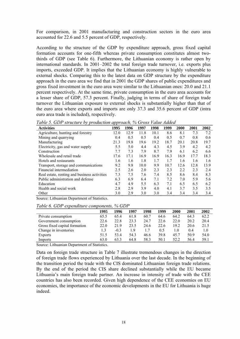
For comparison, in 2001 manufacturing and construction sectors in the euro area accounted for 22.6 and 5.5 percent of GDP, respectively.

According to the structure of the GDP by expenditure approach, gross fixed capital formation accounts for one-fifth whereas private consumption constitutes almost two-thirds of GDP (see Table 6). Furthermore, the Lithuanian economy is rather open by international standards. In 2001–2002 the total foreign trade turnover, i.e. exports plus imports, exceeded GDP. It implies that the Lithuanian economy is highly vulnerable to external shocks. Comparing this to the latest data on GDP structure by the expenditure approach in the euro area we find that in 2001 the GDP shares of public expenditures and gross fixed investment in the euro area were similar to the Lithuanian ones: 20.0 and 21.1 percent respectively. At the same time, private consumption in the euro area accounts for a lesser share of GDP, 57.3 percent. Finally, judging in terms of share of foreign trade turnover the Lithuanian exposure to external shocks is substantially higher than that of the euro area where exports and imports are only 37.3 and 35.6 percent of GDP (intra euro area trade is included), respectively.

Table 5. GDP structure by production approach, % Gross Value Added Activities 1995 1996 1997 1998 1999 2000 2001 2002 Agriculture, hunting and forestry 12.0 12.9 11.8 10.1 8.6 8.1 7.3 7.2 Mining and quarrying 0.4 0.5 0.5 0.4 0.5 0.7 0.8 0.6 Manufacturing 21.3 19.8 19.6 19.2 18.7 20.1 20.8 19.7 Electricity, gas and water supply 5.5 5.0 4.4 4.3 4.5 3.9 4.2 4.2 Construction 7.7 7.3 7.9 8.7 7.9 6.1 6.2 6.6 Wholesale and retail trade 17.6 17.1 16.9 16.9 16.3 16.9 17.7 18.3 Hotels and restaurants 1.6 1.6 1.8 1.7 1.7 1.6 1.6 1.6 Transport, storage and communications 9.2 9.8 10.0 9.9 10.7 12.6 12.8 13.9 Financial intermediation 2.5 2.6 2.0 2.3 2.3 2.2 2.3 2.4 Real estate, renting and business activities 7.3 7.5 7.6 7.4 8.5 8.6 8.4 8.3 Public administration and defense 6.3 6.9 6.4 7.1 7.2 7.0 5.9 5.6 Education 4.7 4.9 5.5 6.3 7.1 6.5 6.5 6.2 Health and social work 2.8 2.9 3.9 4.0 4.1 3.7 3.5 3.5 Other 3.0 2.9 3.0 3.0 3.4 3.4 3.4 3.4

Source: Lithuanian Department of Statistics.

Table 6. GDP expenditure components, % GDP 1995 1996 1997 1998 1999 2000 2001 2002 Private consumption 65.5 65.4 61.8 60.7 64.6 64.2 64.3 62.2 Government consumption 22.6 22.8 23.3 24.7 22.6 22.0 20.2 20.4 Gross fixed capital formation 22.0 21.9 23.5 24.6 22.6 19.2 20.6 21.5 Change in inventories 1.3 -0.3 1.9 1.7 0.5 1.0 0.4 1.0 Exports 51.5 53.4 54.3 46.6 39.8 45.7 50.9 54.0 Imports 63.0 63.3 64.8 58.3 50.1 52.2 56.4 59.1

Source: Lithuanian Department of Statistics.

Data on foreign trade structure in Table 7 illustrate tremendous changes in the direction of foreign trade flows experienced by Lithuania over the last decade. In the beginning of the transition period the trade with the CIS dominated Lithuanian foreign trade relations. By the end of the period the CIS share declined substantially while the EU became Lithuania’s main foreign trade partner. An increase in intensity of trade with the CEE countries has also been recorded. Given high dependence of the CEE economies on EU economies, the importance of the economic developments in the EU for Lithuania is huge indeed.

18

Table 7. Foreign trade structure by major trade partners, % CIS EU CEE USA Other Exports Imports Exports Imports Exports Imports Exports Imports Exports Imports1991 85.9 83.8 3.0 2.6 10.0 4.0 0.0 1.5 1.1 8.1 1992 65.6 79.1 19.6 8.6 11.4 3.9 0.3 2.7 3.1 5.7 1993 57.1 67.5 19.7 21.9 17.7 5.0 0.3 1.2 5.3 4.4 1994 46.7 50.2 30.1 32.3 18.3 12.0 0.6 2.0 4.3 3.5 1995 42.3 42.0 36.4 37.1 14.7 13.1 0.7 1.9 5.9 5.8 1996 45.4 32.9 32.9 42.4 16.2 14.9 0.8 2.3 4.7 7.5 1997 46.4 29.3 32.5 46.5 14.6 15.6 1.6 2.4 5.0 6.3 1998 35.7 24.7 38.0 50.2 17.8 16.9 2.8 2.6 5.7 5.7 1999 18.2 23.6 50.1 49.7 21.2 18.0 4.4 2.9 6.1 5.8 2000 16.3 30.7 47.9 46.5 24.3 15.7 4.9 1.5 6.7 5.7 2001 19.7 28.3 47.8 48.0 23.3 16.0 3.8 1.9 5.4 5.9 2002 19.8 25.3 49.1 49.4 18.8 16.1 3.6 1.4 8.8 7.9 Source: Lithuanian Department of Statistics

The country composition of Lithuania’s foreign trade does not, however, match its currency structure (see Table 8). While the US share in Lithuanian foreign trade remains well below the 5 percent level, up until 2002 the US dollar was the dominant currency in Lithuania’s foreign trade transactions. The popularity of the US dollar can be attributed to the prolonged period of the litas fixed exchange rate regime vs. the US dollar and a large trade share with the CIS countries where the US dollar traditionally has been the main currency of reference. The recent data reveal the increasing role of the EU currencies in Lithuania’s foreign trade. In fact by the end of 2002 the share of EU currencies exceeded that of the US dollar in Lithuania’s imports.17 The other currencies accounted for less than 4 percent.

Table 8. Lithuanian imports’ structure by major currencies, % EU currencies US dollar Lithuanian litas CIS currencies Other currencies1996 29.3 62.2 2.0 3.4 3.1 1997 33.1 60.3 1.3 2.2 3.2 1998 37.9 55.9 0.7 1.5 4.0 1999 37.0 56.7 1.0 1.2 4.1 2000 37.1 57.5 1.5 1.0 2.8 2001 42.5 52.9 1.2 0.6 2.8 2002 53.4 42.9 1.3 0.5 1.9 Source: Lithuanian Department of Statistics

Finally, an important aspect of the Lithuanian transition is the significance of international financial flows for the domestic economy, in particular foreign direct investment (FDI). As shown in Table 9, by the end of 2002 Lithuania managed to attract a large stock of FDI: over a quarter of GDP, mainly through the privatisation process. The country composition of the FDI stock shows that the EU is the most important provider of the FDI in Lithuania with roughly two thirds of the total FDI stock at the end of 2002. The share of the FDI stock stemming from the CEE countries grew substantially from below 3 percent in 1996 to almost 14 percent within five years while the corresponding share of the US shrank from 29 to 8 percent. The CIS share in the FDI stock has remained very low.18

17 Due to data reliability problems we do not report Lithuanian exports structure by currencies. 18 The latter can be partially explained by a (politically motivated) reluctance of the Lithuanian Government to allow Russian capital to participate in the privatization of Lithuanian companies. However,

19

Table 9. Foreign direct investment stock by major countries, %, end of the period EU CEE† CIS US Norway Switzerland Other Total, % GDP

1996 58.2 2.7 2.1 28.5 1.6 2.5 4.4 8.9 1997 57.2 6.1 1.7 25.9 1.6 3.1 4.4 10.9 1998 61.3 7.0 2.2 18.7 1.7 4.2 5.0 15.1 1999 63.2 7.1 1.9 13.4 5.5 3.8 5.1 19.3 2000 64.3 9.9 1.3 9.8 4.8 4.3 5.6 20.7 2001 64.1 13.6 1.7 8.3 3.2 3.7 5.3 22.2 2002 59.5 15.5 5.3 8.7 2.8 2.9 5.3 26.0

Source: Lithuanian Department of Statistics Note: † – Estonia, Latvia, Poland, and Czech Republic.

We can draw several conclusions from the above analysis, which have implications for the MTM in Lithuania. First of all, the industry composition of the domestic economy and aggregate demand structure indicates a significant share of capital-intensive components. The latter argues in favour of the interest rate and credit channels in Lithuania. On the other hand, we find that the Lithuanian economy is highly open and, thus, vulnerable to the external environment. Therefore, when modelling the MTM we need to account for such exogenous variables as foreign prices, income and exchange rate. Finally, a more detailed investigation of the country and currency structure of the Lithuanian foreign trade and financial flows reveals the growing importance of the EU and CEE region for the Lithuanian economy.

3. Empirical Analysis of the MTM in Lithuania

3.1. Identification of the Main Transmission Channels

Figure 6 displays a simple scheme of the monetary transmission mechanism for Lithuania. It captures the main implications of the monetary policy regime employed at present in Lithuania. The CBA environment and no active interest rate policy on the BoL side imply that retail bank rates in Lithuania are largely determined by foreign base interest rates (in particular, by the US dollar (until February 2002) and euro (starting from February 2002) money market rate), and risk premiums. Changes in the foreign interest rate are expected to translate to the domestic interest rate and then to the spending decisions of the Lithuanian households and firms. This mechanism describes the operation of the interest rate channel.

The bank-lending channel operates through the money stock. Changes in money stock affect supply of credit, which in turn induces changes in domestic expenditures. Domestic banks decide how much to lend to the Government, invest abroad, and lend to the domestic corporate sector and households. Thus, shocks to direct Government borrowing and relative profitability of investing abroad largely affect the stock of private credit supplied in Lithuania.

The exchange rate channel describes the response of the Lithuanian economy to shocks to the nominal exchange rate of the litas. Although one bilateral exchange rate is fixed, the effective (foreign trade weighted) exchange rate of the litas is far from stable. The in the first half of 2002 large stakes in the oil-refinery “Mažeikių Nafta” and the Lithuanian gas company “Lietuvos Dujos” were offered to the Russian companies as well, thus, recognizing the importance of securing a stable supply to the production of the privatized companies.

20

effective exchange rate can influence domestic inflation both through import prices and through the effects of foreign trade on the GDP.

Expectations have been an integral part of the Lithuanian MTM. Past and recent experience reveals that the credibility of monetary policy has a direct impact on inflationary expectations. The establishment of the CBA in Lithuania was expected to reduce fears of devaluation and, therefore, also to reduce inflationary expectations; in practice, however, the Lithuanian CBA suffered from a low level of credibility for quite some years following its introduction. This was due to a number of factors, of which excessive politicisation of the CBA and lax fiscal policies were the most important. More recently, however, the credibility of the CBA in Lithuania has been strengthening. The latter is due to improved fiscal and external balances, the successful re-peg of the litas to the euro and the authorities’ chosen exit strategy from the CBA, which supposes maintaining the current CBA until entering the EU and joining ERM 2. The authorities have also expressed an intention of using the euro peg based CBA as a compatible strategy to the ERM 2 until entering the euro area (Kregdždė, 2001).

Figure 6. The transmission mechanism in Lithuania

Currency board

Expected inflation

Domestic

Supply of credit

Money Demand

Foreign money market rate

Output Aggregate

Domestic retail interest rate

Bilthe

Government borrowing

For ttraditthe fmode

Domestic T-bill rate

inflation gap demand

ateral exchange rate: litas vs. the USD/EUR

Foreign prices

Import prices Nominal effective exchange rate

Real effective exchange rate

Aggregate output

he rest, our empirical model will explicitly illustrate the operation of the three ional MTM channels in Lithuania: interest rate, bank lending, and exchange rate. In ollowing we turn to the core equations comprising a small structural econometric l, which we apply to investigate the MTM in Lithuania.

21

3.2. Model Specification and Estimation19

The econometric methodology employed resembles the equilibrium correction (EC) approach. Due to insufficient numbers of observations we use the Engle-Granger two-step procedure. Although in some instances shorter/longer samples were utilized, in general the time series used for model estimation are from 1995 1st quarter to 2001 4th quarter, i.e. only 28 observations. The total number of variables used in the model is 66: 40 endogenous and 26 exogenous (of which there are 8 dummies and a time trend). The list of model’s variables containing their shortened names and description is in the Appendix 3. The empirical model contains 40 equations: 26 stochastic equations and 14 definitions/identities.

To facilitate exposition of the model for each variable we write, first, the static (long run relationship) equation; second, the dynamic (short run relationship) equation follows. The latter incorporates information about the long run relationship in the form of an equilibrium correction term. Small letters “a” and “b” mark the static and dynamic equations correspondingly. For example, for variables zt and xt we write:

zt =α1+ α2·xt [0a]

∆zt =-β1·ec_zt-1+β2·∆xt [0b]

In equation [0b] ec_zt-1= zt-1-α1-α2·xt-1 is the equilibrium correction term lagged by one period.

Time series with a clear seasonal pattern are seasonally adjusted applying the census x-11 procedure. The econometric estimations and model simulations are conducted using the EViews 4.0 package. In each stochastic equation the numbers in parenthesis are t-values of the corresponding estimated coefficients. Goodness of fit of the model's individual equations (adjusted R2) is also reported.

Money market rate

The money market rate in Lithuania is determined by the US dollar money market rate and the Lithuanian Government short-term t-bill rate. The unit coefficient of the t-bill rate in the equation in levels implies the full pass through of the corresponding shock in the long run. The equations are estimated over the period from 1997 1st quarter to 2002 4th quarter. vilibort=tbt+0.284·i_ust R2=0.92 [1a] (6.29) ∆vilibort=-0.809·ec_vilibort-1+1,134·∆tbt R2=0.88 [1b] (-2.58) (7.30)

Bank loan rates

The most important domestic interest rate in our empirical model is the bank loan rate. It reflects the marginal price of the domestic financial resources faced by Lithuanian companies and households. To account for significant dollarization of the Lithuanian

19 The construction of the MTM model for Lithuania benefited greatly from Sepp and Randveer(2002), Pikkani(2001) and Fagan et al(2001). An earlier attempt to construct an MTM model for Lithuania can be found in Kuodis and Vetlov(2002).

22

economy we model both litas denominated and foreign currency denominated bank loan interest rates. In each case, we estimate equations for short-term (up to 1 year) and long-term (over 1 year) loan interest rates. The period of estimation is from 1997 1st quarter to 2002 4th quarter.

In equilibrium the long-term foreign currency bank loan rate adjusted for the country (system) risk premium is equal to the US interest rate. The long-term bank foreign currency loan rate appears to be closer than the short-term bank foreign currency loan rate linked to the US dollar money market rate. In practice, the long-term bank foreign currency loan rate has been directly linked to the US dollar money market rate via mark-up pricing type bank loan contracts. Over the period of estimation the Lithuanian risk premium gradually declined reflecting Lithuania’s achievements in macroeconomic stabilization, market reforms, and accession to the EU. Thus, the risk premium is a complex function containing both economic and political variables. In this paper we treat the risk premium component as given exogenously and proxy it by an inverse linear time trend. The unity coefficient of the foreign interest rate in the equation in levels implies the full pass through of the corresponding shock in the long run. lrfc_lrt= i_ust+2.904+29.1/(trendt) R2=0.90 [2a] (7.43) (4.47) ∆lrfc_lrt=-0.520·ec_lrfc_lrt-1+0.884·∆i_ust R2=0.14 [2b] (-2.48) (3.15)

The short-term bank foreign currency loan interest rate cointegrates with the long-term bank loan interest rate and a constant time premium. lrfc_srt= 1.379+lrfc_lrt R2=0.90 [3a] (9.27) ∆lrfc_srt=-0.598·ec_lrfc_srt-1+0.828·∆lrfc_lr R2=0.70 [3b] (-5.98) (5.57)

The litas bank loan rates are related to their counterparts in foreign currency. In addition, the short-term litas loan interest rates are found to be dependent on the Lithuanian litas money market rate. lrlt_lrt= 3.833+0.633·lrfc_lrt R2=0.80 [4a] (6.08) (9.59) ∆lrlt_lrt=-0.558·ec_lrlt_lrt-1+0.422·∆lrfc_lrt R2=0.36 [4b] (-3.01) (2.63) lrlt_srt=0.885·lrfc_srt+0.264·vilibort R2=0.94 [5a] (19.3) (5.34) ∆lrlt_srt=-ec_lrlt_srt-1+0.793·∆lrfc_sr+0.163·∆vilibort R2=0.75 [5b] (6.50) (3.82)

Finally, average (all currencies) short and long term bank loan interest rates are derived by simple arithmetic average. lr_lrt=(lrfc_lrt+lrlt_lrt)/2 [6] lr_srt=(lrfc_srt+lrlt_srt)/2 [7]

Bank deposit rates

The domestic deposit interest rates are represented by short-term (up to 1 year) and long-term (over 1 year) bank deposit rates. They are the price of domestic financial resources faced by the commercial banks. The period of estimation is from 1997 1st quarter to 2002 4th quarter. The static equation for the short-term deposit rate resembles a mark-up type

23

model. The loan rate coefficient is significantly less than one implying only partial pass through in the long run. The latter could be due to the low level of bank competition in Lithuania observed in the past. The equilibrium relationship between the deposit rate and the loan rate is maintained by adjusting the deposit rate. dr_srt=-1.474+0.614·lr_srt R2=0.96 [8a] (-4.89) (23.6) ∆dr_srt=-0.532·ec_dr_srt-1+0.466·∆lr_srt R2=0.70 [8b] (-3.22) (9.59)

The long-term deposit rate is conditioned by the short-term counterpart and constant time premium. dr_lrt=1.02+0.957·dr_srt R2=0.98 [9a] (6.42) (34.5) ∆dr_srt=-0.717·ec_dr_srt-1+0.933·∆dr_srt R2=0.83 [9b] (-4.18) (12.3)

Aggregate supply

Aggregate supply is specified as an aggregate production function of the Cobb-Douglas functional form with constant returns to scale and the Hicks-neutral technical progress. yst= tfpt·ksrt-1

beta·lnt(1-beta) [10]

Total factor productivity, tfpt, is derived as the Solow residual. beta is equal to average share of income earned by capital (0.35) which is assumed rather than calculated from the System of National Accounts’ statistics (due to poor reliability of the official statistics). Capital stock (ksrt) is estimated applying the Perpetual Inventory Method (PIM): capital stock is equal to the past investments (net of depreciation) plus initial capital stock20.

Capital stock

Capital stock evolves by adding investment net of depreciation21 to the existing capital stock: ksrt=ksrt-1+gfcrt -delta·ksrt-1 [11]

Potential output and the output gap In estimating potentional output it is assumed that the capital stock is at its potential level. Potential employment is the one consistent with NAIRU (non-accelerating inflation rate of unemployment): lntt = lft·(1-urtt) [12]where lntt – is the level of employment consistent with unemployment being at NAIRU, urtt – is time-varying NAIRU. The NAIRU or the long-term unemployment rate is derived using a simple Prior Consistent filter in a state space modelling framework (Kalman filter) (for explanations see Box 7, page 30-31 in Laxton et al (1998) and numerous applications are in Coats et al (2003)). Trend total factor productivity tfptt has been estimated by applying the HP filter to the Solow residual. The potential output yrpott and output gap yrgapt are then calculated as follows: 20 Equation [10] does not enter the model explicitly. 21 The rate of depreciation delta is assumed to be constant at 2.5 percents of the capital stock per quarter.

24

yrpott=tfptt ·(ksrt-1)beta·(lntt)(1-beta) [13]yrgapt=(yrt -yrpott)/yrpott [14]

The details regarding the procedure for deriving the capital stock time series, estimation of the total factor productivity and potential output are left for Appendix 2.

Aggregate demand

Aggregate demand is obtained by summing up GDP expenditure components: private consumption, public consumption, gross fixed capital formation, changes in stocks, and net exports. Public consumption and changes in stocks are treated as exogenous. yrt=crt+grt+gfcrt+invrt+exrt-imrt [15]

Private consumption

The private consumption equation is basically in line with the life cycle theory of consumption, namely, households consume both out of the current disposable income and accumulated wealth. As a proxy for the households’ disposable income we use the nominal GDP deflated by the private consumption expenditure deflator. ydrt=yt/cpt [16]

Households’ wealth is constructed by summing the stock of capital22 and net financial wealth. The latter is proxied by broad money aggregate net of outstanding loan stock (extended to businesses and households). To arrive at a real wealth figure the private consumption expenditure deflator is used. whrt=(ksrt·ipt+m2t-loant)/cpt [17]

The level of the private consumption is also found positively dependent on bank loans creation. The positive credit quantity effects on private consumption to a large extent reflect the fact that the Lithuanian households have been credit constrained. The short run dynamics also reveals importance of changes in the nominal loan rate and real public consumption for the private consumption growth. The public consumption has a significant negative coefficient pointing in the direction of the crowding-out effects of the latter on private expenditures. Its significance can be also explained by the application of a rather imprecise measure of the households’ disposable income. log(crt)=0.674·log(ydrt)+0.233·log(whrt)+(1-0.674-0.233)·∆log(loant/cpt) R2=0.97 [18a] (10.7) (4.39) ∆log(crt)=-0.557·ec_crt-1+0.370·∆log(ydrt)+0.240·∆log(whrt)+ (-3.64) (2.81) (2.31) +0.148·∆log(loant/cpt)-0.006·∆(lr_srt)-0.103·∆log(grt) (2.06) (-2.27) (-2.86) R2=0.65 [18b]

Gross fixed capital formation

Investment is positively related to creation of new loans, real GDP and flow of foreign direct investment into Lithuania. The long-term bank loan interest rate enters with a negative coefficient in the long run relationship. A rising interest rate increases the opportunity costs of financial resources and results in fewer investment projects undertaken. In the dynamic equation the first dummy variable accounts for a sudden decline in investment in the second quarter 2001. The second dummy reflects the increase 22 We assume that households are the sole owners of the capital.

25

in investment induced by the approaching expiration of the tax exemption on reinvested corporate profits (starting from January 2002). log(gfcrt)=0.867·log(yrt)-0.011·(lr_lrt)+0.546·∆log(fdit/ypt)+∆log(loant/ypt) R2=0.91 [19a] (172) (-3.30) (2.56) ∆log(gfcrt)=-0.885·ec_gfcrt-1+0.015+0.608·∆∆log(loant/ypt)+0.257·∆∆log(fdit/ypt)+ (-6.67) (2.43) (3.41) (2.00) +0.444·∆log(yrt)-0.139·din1t+0.070·din2t R2=0.78 [19b] (1.73) (-4.38) (2.10)

Exports

To investigate the exchange rate channel in full, Lithuanian exports are explicitly modelled. As follows from equation [20a], exports depend on the real effective exchange rate (defined in US$ terms), foreign income, and domestic investment. The first two variables are conventional demand side factors of exports, while domestic investment is a supply side factor: increases in investment are associated with higher productivity, more competitive production capacity and, therefore, better export performance in the long run. As a proxy for foreign demand we use the EU GDP. The dummy variable reflects the rapid increase in the world oil price in 1999. log(exrt)=5.299-0.819·log(reert)+3.134·log(yr_eut)+0.903·log(gfcrt)-0.134·doilt R2=0.89 [20a] (6.88) (-4.59) (5.50) (8. 98) (-3.67) ∆log(exrt)=-0.826·ec_exrt-1-0.574·∆log(reert)+3.300·∆log(yr_eut-1)+0.712·∆log(gfcrt) (-4.21) (-2.39) (2.91) (4.99) -0.163·∆(doilt) R2=0.65 [20b](-5.24)

Imports

The long run equation for Lithuanian imports relates the latter to the components of the domestic and foreign demand. The significance of the export expenditures is due to presence of substantial re-export activities in Lithuania. It is especially true for such transitory commodities as oil and oil related products and used cars. Gross investment explains a bulk of imports as well. The latter can be attributed to the significance of imported investment goods, which is specific to the transition period characterized by capital stock build-up. log(imrt)=-1.899+0.504·log(exrt)+0.318·log(irt)+0.349·log(crt)+0.133·log(grt) R2=0.99 [21a] (-4.312) (15.5) (12.4) (6.04) (3.81) ∆log(imrt)=-0.676·ec_imrt-1+0.408·∆log(exrt)+0.317·∆(irt)+0.436·∆log(crt)+ (-3.51) (10.9) (16.7) (3.80) +0.172·∆log(grt) R2=0.96 [21b] (5.21)

Foreign Direct Investment

We find that there is a long run relationship between real FDI, US GDP, Lithuanian GDP and the real long- term interest rate. Foreign GDP development reflects the external economic environment and better economic performance abroad results in larger FDI inflows into Lithuania. The inclusion of the time trend is motivated by the gradualism of the privatisation process in Lithuania given the fact that the FDI inflows into Lithuania have been predominantly due to selling off the Lithuanian state enterprises to foreign strategic investors. The dummy is included to reflect the privatisation of the Lithuanian Telecommunication Company (Lietuvos Telekomas) in summer 1998.

26

log(fdit/ipt)=-10.29+log(yrt)+log(yr_ust)+0.039·rlr_lrt+0.216·dtelt+0.0423·trendt R2=0.99 [22a] (-378) (5.63) (6.04) (17.3) ∆log((fdit/ipt)/yrt)=-0.730·ec_ fdit-1+4.085·∆log(yr_ust)+3.02·∆log(yr_eut-2)+ (-3.12) (4.29) (2.59) +0.127·∆dtelt+0.026·∆(rlr_lrt) R2=0.64 [22b] (3.20) (3.83)

Money demand (M2)

The demand for real money is given by the equation describing demand for broad money. M2. It follows a standard specification where the demand for money is driven mainly by transaction motive. The time trend included in the cointegrating equation accounts for the gradual deepening of the financial market in Lithuania and increasing institutional credibility of the banking sector. The first dummy variable is due to the banking crisis in 1996 while the second one captures the rapid increase in bank deposits caused by a large government transfer under the Soviet Deposit Restitution Program. log(m2t/cpt)=0.971·log(yrt)+0.025·trendt-0.296·dbct R2=0.98 [23a] (398) (23.8) (-10.7) ∆log(m2t/cpt)=-0.542·ec_m2t-1+0.023+0.269·∆log(yrt)-0.141·∆dbct+0.072·dmt R2=0.65 [23b] (-5.00) (5.03) (1.64) (-5.70) (3.03)

Bank lending

Real bank lending measures outstanding bank claims on the private sector and state non-financial enterprises. It increases with the real money stock and the spread between domestic bank loan rate and foreign interest rate. Increases in broad money allow for more lending domestically. The interest rate spread shows the alternative costs of lending abroad vs. domestically. An additional variable included in the current specification is central government borrowing. As we noted in the section on the financial market, the Government is an important borrower in Lithuania. We expect central government borrowing to produce some crowding out of bank lending to other sectors. log(loant/ipt)=log(m2t/ipt)+0.007·(lrfc_srt-i_ust)-0.072·log(govt/ypt) R2=0.96 [24a] (5.29) (-35.3) ∆log(loant/ipt)=-0.196·ec_loant-1+0.778·∆log(m2t/ipt)-0.074·∆log(govt/ypt)+ (-1.95) (7.81) (-2.75) +0.249·∆log(loant/ipt) R2=0.69 [24b] (2.50)

Real effective exchange rate

The real effective exchange rate is CPI based. In specifying the equation we rely on one of the widely known economic theories explaining movements in the CPI based real exchange rates: the Balassa-Samuelson effect. We assume that prices in the tradable sector are determined by foreign prices. Furthermore, to capture relative productivity in the tradable sector vs. non-tradable sector we use the Lithuanian CPI to foreign CPI (given by the EU CPI) ratio. The nominal exchange rate is included in the equation to account for exogenous shocks to the nominal exchange rate. log(reert)=1.967+log(cpit/cpi_eut)+0.406·log(neert) R2=0.99 [25a] (32.6) (43.5) ∆log(reert)=-0.333·ec_reert-1+0.614·∆log(neert)+0.785·∆log(cpit/cpi_eut)- 0.009 R2=0.92 [25b] (-12.2) (15.9) (7.53) (-3.38)

27

Nominal effective exchange rate

The nominal effective exchange rate is a weighted average of the litas nominal effective exchange rate with respect to the EU, CIS, CEE currencies, and the US. The sum of these four coefficients is restricted to unity. Ideally, the estimates of the coefficients must indicate the relative importance of the respective country groups in Lithuanian foreign trade. However, the construction of the nominal effective exchange rate of the litas is based on the (quarterly) changing trade weight system, therefore, the regression below shows period (from 1996 1st quarter to 2002 4th quarter) averages rather than the current foreign trade structure. The equation is estimated merely for analytical convenience. It allows us studying the response of the model to four exchange rate shocks separately.

log(neert)=0.498+0.276·log(neer_eut)+0.346·log(neer_cist)+0.321·log(neer_ceet) (41.9) (6.85) (111) (6.76) +(1-0.276-0.346-0.321)·log(er_ust) R2=1 [26a]

Prices

The price block consists of nine equations describing the behaviour of the consumer, producer, import price indices, the GDP deflators, and the wages. The oil related items constitute roughly one-fifth of the official producer and import price indices, thus, bringing large swings in the data following the oil price changes in the international markets. At the same time the consumer price index and the GDP deflator were found far less dependent on oil price fluctuations, partly due to the smaller weight of oil related items in the their structure. Thus, we excluded oil related items from the producer and import price indices. The log-linear trend is included in price equations and reflects the gradual convergence process of the Lithuanian price level to the western one.

Consumer Price Index

In equilibrium the consumer price index is determined by the producer and import price indices. The dynamics of the CPI depends on the deviation from the equilibrium relationship, changes in the PPI, foreign inflation (in this case the EU inflation), and the output gap lagged by two quarters. log(cpit)=-0.065+0.155·log(trendt)+0.272·log(mpioxt)+0.279·log(ppioxt) R2=0.99 [27a] (-4.36) (8.1) (2.13) (1.58) ∆log(cpit)=-0.465·ec_cpit+∆log(cpi_eut)+0.468·∆log(cpit-1)+0.492·∆ppioxt (-4.31) (10.2) (5.63) +0.105·yrgapt-2 R2=0.97 [27b] (4.48)

Producer Price Index

The static equation for the producer price index describes the relationship between the producer price index, import prices and the world price of oil. The log-linear time trend is included to capture the price convergence process. In the dynamic equation we included a dummy for the increase in the excise tax on petrol, alcohol, tobacco and tariffs of administrated goods and services (water supply, heating, and telecommunication services) in 1997 3 quarter. log(ppioxt)=0.07+0.108·log(trendt)+0.771·log(mpioxt)+0.04·log(poilt) R2=0.97 [28a] (7.97) (28.2) (15.7) (3.66) ∆ppioxt=-0.480·ec_ppioxt-1+0.262·∆log(mpioxt)+0.282·∆log(ppioxt-1)+ (-2.93) (3.27) (2.13)

28

+0.198·∆log(ppioxt-4)+0.023·∆log(poilt)+0.017·dippt R2=0.82 [28b] (2.44) (2.49) (3.27)

Import Price Index

The main determinants of import prices in Lithuania are foreign prices and the nominal exchange rate. Bearing in mind the Lithuanian trade structure by country as a proxy for foreign prices we use the EU CPI. The point estimates of the exchange rate coefficients suggest that the impact of the litas exchange rate versus the EU currencies is significantly larger than that versus the CIS countries. log(mpioxt)=2.426+log(cpi_eut)-0.421·log(neer_eut)-0.08·log(neer_cist)+ (7.44) (-5.19) (-7.13) +0.031·log(trendt) R2=0.90 [29a](2.84)

∆log(mpioxt)=-0.521·ec_mpioxt-1-0.267·∆log(neer_eut)-0.007+∆log(cpi_eut) R2=0.51 [29b] (-4.3) (-3.49) (-2.61)

Private consumption deflator

The private consumption deflator is intimately related to the CPI. Thus, the CPI is the main and only explanatory variable. The equation is estimated over the period from 1996 1 quarter to 2002 3 quarter. As follows from the equations below we find a one-to-one relationship between the price indices. Significance of the constant term in the cointegrating relationship can be attributed to different weight structures of the price indices. log(cpt)=-0.161+log(cpit) R2=0.93 [30a] (-82.9) ∆log(cpt)=-0.756·ec_cpt-1+∆log(cpit) R2=0.55 [30b] (-6.48)

Public consumption deflator

Given the fact that a bulk of the public current expenditures is salary bills of the civil servants we relate the public consumption deflator to wages. In the dynamic equation the growth in the public consumption deflator depends on wage growth: both contemporaneous and lagged by four quarters. Significance of lagged wage growth in the dynamic equation can be attributed to the specifics of the slow budgetary adjustments. log(gpt)=-3.522+0.542·log(wt)+0.134·log(trendt) R2=0.99 [31a] (-8.89) (7.79) (5.04) ∆log(gpt)=-0.460·ec_gpt-1+0.355·∆log(wt)+0.277·∆log(wt-4) R2=0.58 [31b] (-2.43) (2.32) (2.55)

Investment deflator

The investment deflator is determined by the prices of imported and domestic commodities. log(ipt)=0.792·log(mpioxt)+0.435·log(ypt) R2=0.88 [32a] (11.8) (24.8) ∆log(ipt)=-0.762·ec_ipt-1+0.553·∆log(mpioxt)+0.479·∆log(ypt) R2=0.56 [32b] (-3.96) (2.66) (4.52)

29

Export deflator

The export deflator is explained by the PPI (oil excluded) and oil price index. The importance of the latter stems from the fact that oil products account for roughly one fifth of the Lithuanian commodity exports. log(xpt)=-0.089+0.617·log(ppioxt)+0.142·log(poilt) R2=0.85 [33a] (-4.33) (8.73) (7.92) ∆log(xpt)=-ec_xpt-1+0.073·∆log(poilt)+0.278·∆log(xpt-1)+0.069·dxpt R2=0.80 [33b] (2.63) (2.84) (3.76)

Import deflator

The import deflator is determined by the import price index (oil excluded) and oil world price index. log(mpt)=0.009+0.509·log(mpioxt)+0.121·log(poilt) R2=0.91 [34a] (3.78) (15.7) (12.9) ∆log(mpt)=-0.523·ec_mpt-1+0.576·∆log(mpioxt)+0.094·∆log(poilt)+ (-3.32) (7.60) (7.01) +0.175·∆log(mpt-1) R2=0.85 [34b] (2.16)

Wages

In the long run real wages are expected to co-integrate with apparent labour productivity given by the GDP to employment ratio. The dynamic wage equation is based on the Phillips curve where nominal wage growth reacts negatively to the one period lagged spread between the actual unemployment rate and the NAIRU. log(wt)=-1.928+log(ypt)+log(yr/lnt) R2=0.86 [35a] (-129) ∆log(wt)=-0.333·ec_wt-1+0.343·∆log(yp)+0.348·∆log(yrt/lnt)-1.62·(urt-1- urtt-1)+ (-8.52) (2.75) (4.07) (-8.95) +0.031 R2=0.86 [35b] (8.30)

Labour demand Labour demand is obtained by linking the unemployment gap (i.e. the spread between the NAIRU and the actual unemployment rate) to the output gap. From equation [36], actual unemployment is equal to the NAIRU in equilibrium. The level of employment is derived through a trivial identity, [37]. The labour force and the NAIRU unemployment are exogenous by assumption. urt= urtt+0.889·(urt-1- urtt-1)-0.086*yrgapt (19.5) (-3.90) R2=0.98 [36] lnt=lft·(1-urt) [37]

Other definitions and identities yt=crt·cpt+grt·gpt+gfcrt·ipt+exrt·xpt-imrt·mpt+invt [38]ypt=yt/yrt [39]rlr_lrt=100·{(1+lr_lrt/100)0.25-1-(ipt/ipt-4-1)/4} [40]irt=gfcrt+invrt [41]

30

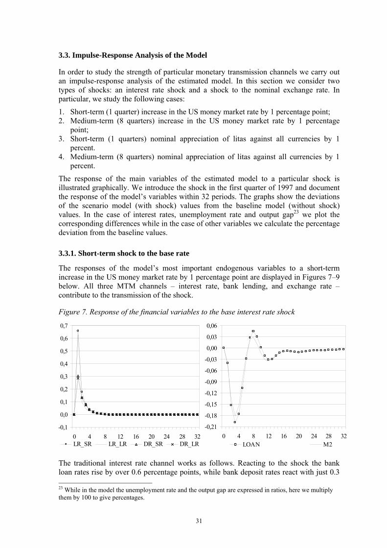
3.3. Impulse-Response Analysis of the Model

In order to study the strength of particular monetary transmission channels we carry out an impulse-response analysis of the estimated model. In this section we consider two types of shocks: an interest rate shock and a shock to the nominal exchange rate. In particular, we study the following cases:

1. Short-term (1 quarter) increase in the US money market rate by 1 percentage point; 2. Medium-term (8 quarters) increase in the US money market rate by 1 percentage

point; 3. Short-term (1 quarters) nominal appreciation of litas against all currencies by 1

percent. 4. Medium-term (8 quarters) nominal appreciation of litas against all currencies by 1

percent.

The response of the main variables of the estimated model to a particular shock is illustrated graphically. We introduce the shock in the first quarter of 1997 and document the response of the model’s variables within 32 periods. The graphs show the deviations of the scenario model (with shock) values from the baseline model (without shock) values. In the case of interest rates, unemployment rate and output gap23 we plot the corresponding differences while in the case of other variables we calculate the percentage deviation from the baseline values.

3.3.1. Short-term shock to the base rate

The responses of the model’s most important endogenous variables to a short-term increase in the US money market rate by 1 percentage point are displayed in Figures 7–9 below. All three MTM channels – interest rate, bank lending, and exchange rate – contribute to the transmission of the shock.

Figure 7. Response of the financial variables to the base interest rate shock

-0,1

The traditional interest rate channel works as follows. Reacting to the shock the bank loan rates rise by over 0.6 percentage points, while bank deposit rates react with just 0.3 23 While in the model the unemployment rate and the output gap are expressed in ratios, here we multiply them by 100 to give percentages.

0,0

0,1

0,2

3

4

0,5

0,6

7

0 4 8 12 16 20 24 28 32

0,

0,

0,

LR_SR LR_LR DR_SR DR_LR

-0,21

-0,18

-0,15

-0,12

-0,09

-0,06

-0,03

0,00

0,03

0,06

0 4 8 12 16 20 24 28 32LOAN M2

31

percentage points. The rise in bank rates depresses private consumption and investment. The first variable bottoms in the first quarter at 0.47 percent, while the second one reaches the bottom in the second quarter at 0.89 percent. The decline in investment cuts export capabilities and exports fall by 0.6 percent. Overall, GDP declines by approximately 0.25 percent in the second quarter before returning to the baseline in the subsequent periods.

Domestic recession results in a smaller money stock and a consequently thinner loan portfolio. Both variables reach the bottom in the third quarter with 0.18 and 0.20 percent respectively. It is noteworthy, that the loans also decline due to widening in the spread between foreign and domestic interest rates. The decline in real loans in turn leads to smaller domestic expenditures (the bank lending channel).

Turning to the supply side, the decline in investment results in shrinking capital stock (declines by 0.06 percent within one year), which in turns induces lower potential output. The adjustment in the capital stock and hence in potential output is very sluggish. This partly can be attributed to a missing link which has not been introduced into the model yet, namely the relationship between the marginal product of capital and the desired capital stock. As we will see in medium term interest rate shock scenario later, the output gap does not fully close within 8 years due to sluggishness in potential output.

Figure 8. Response of the real sector variables to the base interest rate shock

-0,9-0,8-0,7-0,6-0,5-0,4-0,3-0,2-0,10,00,1

0 4 8 12 16 20 24 28 32YR CR GFCREXR IMR

-0,08

-0,04

0,00

0,04

0,08

0,12

0,16

0,20

0 4 8 12 16 20 24 28 32WHR KSRLN YRPOTREAL_FDI

-0,16

-0,14

-0,12

-0,10

-0,08

-0,06

-0,04

-0,02

0,00

0,02

0 4 8 12 16 20 24 28 32REAL_W REER

-0,30

-0,25

-0,20

-0,15

-0,10

-0,05

0,

00

05

10

0 4 8 12 16 20 24 28 32

0,

0,

UR YRGAP

32

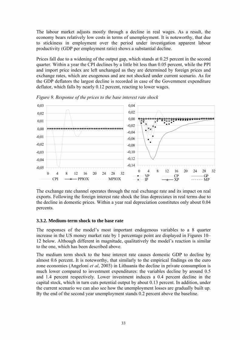
The labour market adjusts mostly through a decline in real wages. As a result, the economy bears relatively low costs in terms of unemployment. It is noteworthy, that due to stickiness in employment over the period under investigation apparent labour productivity (GDP per employment ratio) shows a substantial decline.

Prices fall due to a widening of the output gap, which stands at 0.25 percent in the second quarter. Within a year the CPI declines by a little bit less than 0.05 percent, while the PPI and import price index are left unchanged as they are determined by foreign prices and exchange rates, which are exogenous and are not shocked under current scenario. As for the GDP deflators the largest decline is recorded in case of the Government expenditure deflator, which falls by nearly 0.12 percent, reacting to lower wages.

Figure 9. Response of the prices to the base interest rate shock

-0,05

-0,04

-0,03

-0,02

-0,01

The exchange rate channel operates through the real exchange rate and its impact on real exports. Following the foreign interest rate shock the litas depreciates in real terms due to the decline in domestic prices. Within a year real depreciation constitutes only about 0.04 percents.

3.3.2. Medium-term shock to the base rate

The responses of the model’s most important endogenous variables to a 8 quarter increase in the US money market rate by 1 percentage point are displayed in Figures 10–12 below. Although different in magnitude, qualitatively the model’s reaction is similar to the one, which has been described above.

The medium term shock to the base interest rate causes domestic GDP to decline by almost 0.6 percent. It is noteworthy, that similarly to the empirical findings on the euro zone economies (Angeloni et al, 2003) in Lithuania the decline in private consumption is much lower compared to investment expenditures: the variables decline by around 0.5 and 1.4 percent respectively. Lower investment induces a 0.4 percent decline in the capital stock, which in turn cuts potential output by about 0.13 percent. In addition, under the current scenario we can also see how the unemployment losses are gradually built up. By the end of the second year unemployment stands 0.2 percent above the baseline.

0,00

01

0,02

03

0 4 8 12 16 20 24 28 32

0,

0,

CPI PPIOX MPIOX

-0,14

-0,12

-0,10

-0,08

-0,06-0,04

-0,02

0,00

0,02

0,04

0 4 8 12 16 20 24 28 32YP CP GPIP XP MP

33

Figure 10. Response of the financial variables to the base interest rate shock

-0,1

1,

01234567890

0 4 8 12 16 20 24 28 32

0,0,0,0,0,0,0,0,0,0,

LR_SR LR_LR DR_SR DR_LR

-0,7

-0,6

-0,5

-0,4

-0,3

-0,2

-0,1

0,0

0,1

0 4 8 12 16 20 24 28 32LOAN M2

Figure 11. Response of the real sector variables to the base interest rate shock

Following the interest rate shock the output gap widens and exerts downward pressure on domestic prices. After six quarters following the shock the CPI declines by nearly 0.14 percent. While aggregate demand returns to the baseline by the end of the period

-1,6-1,4-1,2-1,0-0,8-0,6-0,4-0,20,0

2

0 4 8 12 16 20 24 28 32-0,5

-0,4

-0,3

-0,2

-0,1

0,0

0,1

0,2

0,3

0 4 8 12 16 20 24 28 32WHR KSRLN YRPOTREAL_FDI

0,

YR CR GFCREXR IMR

-1,0-0,9-0,8-0,7-0,6-0,5-0,4-0,3-0,2-0,10,00,1

0 4 8 12 16 20 24 28 3REAL_W REER

-0,6

-0,5

-0,4

-0,3

-0,2

-0,1

0,0

0,1

0,2

0 4 8 12 16 20 24 28 32UR YRGAP

2

34

potential output does not, therefore, the output gap remains slightly positive at the end of the simulation period. As a result the CPI is left marginally above the baseline. As in case of the short-term shock scenario the main adjustments to the shock are taking place in the real variables.

Figure 12. Response of the prices to the base interest rate shock

-0,14

-0,12

-0,10

-0,08

-0,06

-0,04

-0,02

3.3.3. Short-term shock to nominal exchange rate Under this scenario the main MTM channel through which the nominal exchange rate shock is transmitted is the exchange rate channel. The model responses to the shock are displayed in Figures 13–15 below. The short-term appreciation of the litas against all currencies by 1 percent produces at bottom a decline of about 0.27 percent in import prices, 0.12 percent in producer prices, and 0.13 percent in the CPI. Figure 13. Response of the financial variables to the litas exchange rate shock The real appreciation of the litas in the first quarter is approximately 0.6 percent, which is smaller than the nominal appreciation due to the contemporaneous fall in the domestic prices. Reacting to lower competitiveness Lithuanian real exports decrease by 0.5

0,00

0,02

04

0 4 8 12 16 20 24 28 32

0,

CPI PPIOX MPIOX

-0,7

-0,6

-0,5

-0,4

-0,3

-0,2

-0,1

0,0

0,1

0 4 8 12 16 20 24 28 32YP CP GPIP XP MP

-0,10,0

12345678901

0 4 8 12 16 20 24 28 32NEER

-0,18-0,16-0,14-0,12-0,10-0,08-0,06-0,04-0,020,000,020,040,06

0 4 8 12 16 20 24 28 32LOAN M2

1,1,

0,0,0,

0,0,0,0,0,0,

35

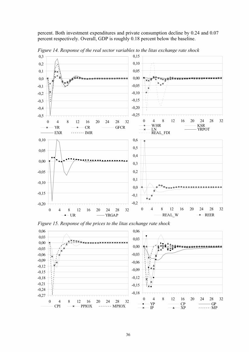
percent. Both investment expenditures and private consumption decline by 0.24 and 0.07 percent respectively. Overall, GDP is roughly 0.18 percent below the baseline. Figure 14. Response of the real sector variables to the litas exchange rate shock Figure 15. Response of the prices to the litas exchange rate shock

-0,5

-0,4

-0,3

-0,2

-0,1

0,0

1

2

3

0 4 8 12 16 20 24 28 32

-0,25

-0,20

-0,15

-0,10

-0,05

0,00

0,05

0,10

0,15

0 4 8 12 16 20 24 28 32WHR KSRLN YRPOTREAL_FDI

0,

0,

0,

YR CR GFCREXR IMR

-0,2

-0,1

0,0

0,1

0,2

0,3

0,4

0,5

0,6

0 4 8 12 16 20 24 28 3REAL_W REER

-0,20

-0,15

-0,10

-0,05

0,

00

05

10

0 4 8 12 16 20 24 28 32

0,

0,

2UR YRGAP

-0,27-0,24-0,21-0,18-0,15-0,12-0,09-0,06-0,03

0,

000306

0 4 8 12 16 20 24 28 32

0,0,

CPI PPIOX MPIOX

-0,18

-0,15

-0,12

-0,09

-0,06

-0,03

0,00

0,03

0,06

0 4 8 12 16 20 24 28 32YP CP GPIP XP MP

36

3.3.4. Medium-term shock to nominal exchange rate

The medium-term appreciation of the litas against all currencies by 1 percent produces at the bottom a decline of about 0.5 percent in import prices, 0.43 percent in producer prices, and 0.36 percent in the CPI (see Figure 18).

Figure 16. Response of the financial variables to the litas exchange rate shock

-0,10,0

Figure 17. Response of the real sector variables to the litas exchange rate shock

0,10,2

30,4

50,6

70,8

91,0

1

0 4 8 12 16 20 24 28 32NEER

-0,50-0,45-0,40-0,35-0,30-0,25-0,20-0,15-0,10-0,050,000,05

0 4 8 12 16 20 24 28 32LOAN M2

1,

0,

0,

0,

0,

-0,7-0,6-0,5-0,4-0,3-0,2-0,10,0,

012

0,3

0 4 8 12 16 20 24 28 32

0,

YR CR GFCREXR IMR

-0,60-0,55-0,50-0,45-0,40-0,35-0,30-0,25-0,20-0,15-0,10-0,050,000,05

0 4 8 12 16 20 24 28 32WHR KSRLN YRPOTREAL_FDI

-0,5-0,4-0,3-0,2-0,10,00,10,20,30,40,50,6

0 4 8 12 16 20 24 28 3REAL_W REER

-0,20-0,18-0,16-0,14-0,12-0,10-0,08-0,06-0,04-0,020,00

2

0,0,0,

020406

0 4 8 12 16 20 24 28 32UR YRGAP

37

The real effective exchange rate contemporaneously appreciates by about 0.6 percent inducing a short run fall in the real exports by 0.63 percent in the second quarter. Exports also react to lower investment induced by the smaller FDI. The latter is due to the deterioration in GDP performance, which within 2 quarters decreases by almost 0.2 percent.

Over quarters 2–5 the real exchange rate gradually depreciates (due to falling domestic prices) bringing the overall level of litas real appreciation to only 0.1 percent. As a result the medium-run response of real exports is also smaller than the initial reaction. Overall, due to overshooting in the real exchange rate the real GDP expenditure reactions exhibits short-term fluctuations.

Figure 18. Response of the prices to the litas exchange rate shock

-0,50-0,45-0,40-0,35-0,30-0,25-0,20-0,15-0,10-0,05

3.4. Shocks compared In this section we are comparing the responses of the key macroeconomic variables to both shocks. Figures 19 and 20 bring together the responses of GDP and CPI to the interest rate and exchange rate shocks. Figure 19. GDP and CPI responses to the short term interest rate and exchange rate shocks +

0,0,0,

000510

0 4 8 12 16 20 24 28 32CPI PPIOX MPIOX

-0,55-0,50-0,45-0,40-0,35-0,30-0,25-0,20-0,15-0,10-0,050,000,050,10

0 4 8 12 16 20 24 28 32YP CP GPIP XP MP

-0,30

,25

,20

,15

,10

,05

00

05

10

0 4 8 12 16 20 24 28 32YR_to_base_rate YR_to_NEER

-0,14-0,12-0,10-0,08-0,06-0,04-0,020,000,020,040,06

0 4 8 12 16 20 24 28 32CPI_to_base_rate CPI_to_NEER

0,

0,

0,

-0

-0

-0

-0

-0

38

Let us first consider the short-term shocks. As follows from Figure 19 under both shocks GDP reacts by the same magnitude in the first quarter. However, when comparing the GDP values at the bottom we find that the interest rate shock results in a reaction in GDP 1.4 times larger. It is noteworthy, that GDP returns to the baseline faster in case of the exchange rate shock as compared to the interest rate shock scenario. At the same time the initial price reaction is faster under the exchange rate scenario (due to contemporaneous effect of the exchange rate on import prices), while prices return to the baseline roughly at the same time. In case of the exchange rate shock, at the bottom the CPI decline will be roughly 2.5 times larger than in the case of the interest rate shock. Figure 20. GDP and CPI responses to the medium term interest rate and exchange rate shocks

Our general observations derived from comparing the variables’ reactions to the short-term shocks can be largely extended to the medium term shocks (Figure 20). We still find that the GDP response is bigger and the CPI response is smaller under the interest rate shock scenario as compared to the exchange rate shock case. However, while the quantitative difference in price reaction (2.6 times) under the two shocks is similar to previous finding, the ratio of the GDP reaction under interest rate and exchange rate shocks is now 2.9 times. The latter can be explained by a much greater response of the domestic prices under exchange rate shock scenario, which significantly reduces the initial real appreciation, thus, lowering the impact of the shock on the GDP.

-0,6

,5

,4

,3

,2

,1

0

1

0 4 8 12 16 20 24 28 32YR_to_base_rate YR_to_NEER

-0,40-0,35-0,30-0,25-0,20-0,15-0,10-0,050,000,050,10

0 4 8 12 16 20 24 28 32CPI_to_base_rate CPI_to_NEER

0,

0,

-0

-0

-0

-0

-0

39

4. Conclusions and Future Research Agenda In this paper we attempted to shed some light on the key issues explaining the peculiarities of the Lithuanian MTM and to identify the transmission channels based on the empirical structural econometric model. In the first part of the paper we find that due to the application of the currency board arrangement the MTM in Lithuania diverges from the usual MTM. The main features of the CBA are a largely automatic money creation rule based on the coverage requirement and ultimately fixed exchange rate against the base currency. The CBA eliminates scope for active domestic monetary policy. On the one hand, money stock is money demand determined, on the other hand, domestic interest rates are governed by the foreign interest rate and may diverge from the latter due to the risk premium.

The analysis of the structure of the domestic financial sector allows us to derive at least three basic conclusions. First, the financial sector in Lithuania remains underdeveloped (narrow and thin). Second, the performance of the market is determined mainly by actions undertaken by commercial banks and the Government. The last, though by no means the least important, conclusion is that the Lithuanian financial market becomes increasingly integrated into the international financial system, which implies larger dependence of Lithuania’s financial sector on the latter. All three conclusions have certain implications for the MTM in Lithuania. On the one hand, an underdeveloped domestic financial market means relatively weak interest rate and bank lending channels. On the other hand, the commercial bank retail interest rate, interest rates paid on Government securities and the foreign money market interest rate are likely to be the key interest rates to be considered when modelling the Lithuanian MTM.

The investigation by the industry composition of the domestic economy and aggregate demand structure reveals a significant share of capital-intensive components. The latter argues for the importance of the interest rate and bank lending channels in Lithuania. On the other hand, we find that the Lithuanian economy is highly open and, thus, vulnerable to the external environment. The latter implies the significance of the exchange rate channel in the Lithuanian MTM. A more detailed analysis of the country and currency structure of the Lithuanian foreign trade and financial flows shows the dominant position of the US dollar historically, at the same time indicating the growing importance of the EU and CEE region for the Lithuanian economy over the last several years.

The empirical structural small-scale model estimated in this paper incorporates three traditional MTM channels: interest rate, bank lending, and exchange rate channels. To illustrate the operation of the above-mentioned MTM channels, two shocks were introduced into the system and two response of the key macroeconomic variables were studied: increase in the US money market rate by 1 percentage point and nominal appreciation of the litas by 1 percent.

The interest rate channel describes the transmission of the monetary policy shock from the foreign money market interest rate to domestic GDP and inflation. The shock to the base rate results in higher domestic bank interest rates. The latter further depresses domestic investment and consumption altering aggregate demand and the output gap. The output gap in turn exercises pressure on domestic prices. It is noteworthy, that similar to the findings on the MTM in the euro area we find that the investment demand in Lithuania is more sensitive than the private consumption to the interest rate shock. In

40

addition, the main burden of the economy’s adjustment to the rate shock is placed on the real variables as opposed to the nominal ones.

The bank-lending channel operates through changes in the money stock and interest rate spread between the domestic bank loan rate and foreign interest rate. Since the money stock is money demand determined, shocks to money demand translate into changes in money stock. The latter has a direct impact on the amount of credit supplied. The spread between domestic bank loan and foreign interest rates also affects the supply of credit: an excess of the domestic interest rate over the foreign one induces a boom of domestic credit while in the opposite case a credit contraction results. Credit supply affects aggregate demand and, thus, constitutes one of the important sources of economic fluctuations in Lithuania.

The exchange rate channel describes both direct (through import prices) and indirect (through output gap) impacts of the exchange rate shock on domestic prices. In the first case, nominal exchange rate changes induce changes in import prices, which directly feed into the domestic producer and consumer prices. In the second case, nominal exchange rate changes bring fluctuations in the real exchange rate, which in turn affects GDP through Lithuanian exports.

Comparison of the model reactions to the interest rate and exchange rate shocks yields some interesting conclusions. First, both under short-term and medium-term shocks the GDP response is greater (1.4 and 2.9 times in case of short-term and medium-term shocks respectively) under the interest rate shock scenario as compared to the exchange rate shock case. It is noteworthy, that GDP returns to the baseline faster in case of the exchange rate shock. Second, the CPI response is larger (2.5 and 2.6 times in case of short-term and medium-term shocks respectively) under the exchange rate shock scenario. At the same time price reaction is faster under the exchange rate scenario (due to contemporaneous effect of the exchange rate on import prices), while prices return to the baseline roughly contemporaneously.

The present study can be further elaborated with particular attention paid to the improvement of the existent equations and bringing in new ones. For example, one straightforward improvement to the model could be to introduce a risk-premium equation that would explain domestic and foreign interest rate spreads explicitly. Bearing in mind the fact that in the first quarter of 2002 the litas was re-pegged to the euro, in order to extend the estimation period forward, some equations need substantial modification. In particular, we need to bring the euro money market rate into the interest rate block. Furthermore, more modelling efforts are required in the case of the investment demand equation as so far we have failed to relate investment demand to the marginal productivity of capital. Finally, we need to introduce links between foreign interest rates, foreign prices and income. Constructing a VAR model for the foreign variables and them adding it to the core MTM structural model can do it.

41

References Angeloni, I., Kashyap, A. and B. Mojon, (2003), Monetary Transmission in the Euro Area, Cambridge

University Press.

Bank of Lithuania, (2002), 2001 Annual Report, Bank of Lithuania, Vilnius.

Bank of Lithuania, (2001), 2000 Annual Report, Bank of Lithuania, Vilnius.

Bank of Lithuania, (2000), 1999 Annual Report, Bank of Lithuania, Vilnius.

Bank of Lithuania, (1999a), Guidelines for the application of the Bank of Lithuania monetary policy instruments: <http://www.lbank.lt/acts/default.asp> (in Lithuanian).

Bank of Lithuania, (1999b), 1998 Annual Report, Bank of Lithuania, Vilnius (in Lithuanian).

Bank of Lithuania, (1998), 1997 Annual Report, Bank of Lithuania, Vilnius (in Lithuanian).

Bank of Lithuania, (1995), Bank of Lithuania 1990–1995, Chief editor V. Terleckas, Bank of Lithuania, Vilnius (in Lithuanian).

Bank of England, (1999), Economic Models at the Bank of England, Bank of England, 156 p.

Bennett, Adam, (1994), ‘Currency Boards: Issues and Experiences’, IMF PPAA, No. 18, International Monetary Fund.

Bernanke B. and M. Gertler, (1995), ‘Inside the Black Box: The Credit Channel of Monetary Policy Transmission’, Journal of Economic Perspectives, Fall, No. 4, pp. 27–48.

Carlino, G. and R. Defina, (1998), ‘Monetary Policy and the US States and Regions: Some Implications for the European Monetary Union’, Federal Reserve Bank of Philadelphia Working Paper, No. 98-97.

Coats, Warren, Douglas Laxton and David Rose, (2003), The Czech National Bank’s Forecasting and Policy Analysis System, Czech National Bank, Prague.

Fagan, G., J. Henry and R. Mestre, (2001), ‘An Area-Wide Model (AWM) for the Euro Area’, ECB Working Paper, No. 42.

Garbaravičius, T. and R., Kuodis, (2002), ‘The Structure and the Functioning of the Financial Sector in Lithuania’, Monetary Studies, Bank of Lithuania, No. 1, pp. 18-47 (In Lithuanian).

Ghosh, A. R., Gulde, Anne-Marie, and Wolf, H. C., (2000), ‘Currency Boards: More Than a Quick Fix? ’, Economic Policy, No. 31, pp. 271-335.

Ho, Corrinne, (2002), ‘A Survey of the Institutional and Operational Aspects of Modern-Day Currency Boards’, BIS Working Paper, No. 110, Bank for International Settlements.

Kamin S., Turner P. and Van’t dack J., (1998), ‘The Transmission Mechanism of Monetary Policy in Emerging Market Economies: An Overview’, BIS Working Paper, Bank for International Settlements, Basle, pp. 5–64.

Kuodis R. and Vetlov, I., (2002), ‘Monetary Transmission Mechanism in Lithuania’, Monetary Studies, VI, No. 3, Bank of Lithuania, (In Lithuanian), pp. 27–63.

Kregdždė, Arvydas, (2001), ‘Why the Fixed Rate Regime Could Be an Appropriate strategy for Integration into the EMU in the Case of Lithuania’, Paper Presented at a Conference Economic Policy in the Framework of Accession to the European Union and Economic and Monetary Union, held in Vilnius, February 8-9, The Lithuanian Banking, Insurance and Finance Institute, pp. 142–147.

Lättemäe, R., (2001), ‘Monetary Transmission Mechanism in Estonia – Some Theoretical Considerations and Stylized Aspects’, Working Papers of Eesti Pank, No. 4, Bank of Estonia.

Laxton, Douglas, Peter Isard, Hamid Faruqee, Eswar Prasad, and Bart Turtleboom, (1998), MULTIMOD Mark III: The Core Dynamic and Steady-State Models, IMF Occasional Paper 164 (Washington: International Monetary Fund).

McAdam, P. and J. Morgan, (2001), ‘The Monetary Transmission Mechanism at the Euro Area level: Issues and Results using Structural Macroeconomic Models’, ECB Working Paper, No. 93.

42

Mishkin, F., (2001), ‘The Transmission Channels and the Role of Asset prices in Monetary Policy’, NBER Working Paper, No. 8617: http://papers.nber.org/papers/W8617.

Mishkin, F., (1996), ‘The Channels of Monetary Transmission: Lessons for Monetary Policy’, NBER Working Paper, No. 5464: http://papers.nber.org/papers/W5464.

Mojon, B. and G. Peersman, (2001), ‘A VAR Description of the Effects of Monetary Policy in the Individual Countries of the Euro Area’, ECB Working Paper, No. 92.

Peersman, G. and F. Smets (2001a), ‘The Monetary Transmission Mechanism in the Euro Area: more evidence from VAR Analysis’, ECB Working Paper, No. 91.

Peersman, G. and F. Smets (2001b), ‘The Industry Effects of Monetary Policy’, mimeo.

Pikkani, R., (2001), ‘Monetary Transmission Mechanism in Estonia – Empirical Model’, Working Papers of Eesti Pank, No. 5, Bank of Estonia.

Romer, David, (1996), Advanced Macroeconomics, The McGraw-Hill Companies, Inc.

Rõõm, Marit, (2001), ‘Potential Output for Central and Eastern European Counties Using Production Function Method’, Working Papers of Eesti Pank, No. 2, Bank of Estonia: <http://www.ee/epbe/papers/2_2001/index.html.en>(October18, 2002).

Sepp, U. and M. Randveer, (2002), ‘Aspects of the Sustainability of Estonian Currency Board Arrangement’, Working Papers of Eesti Pank, No. 5, Bank of Estonia.

Vetlov, I., (2002), ‘Analysis of the Real Exchange Rate and Competitiveness in Lithuania’, In Relationship between Real Exchange Rate and Competitiveness in the Baltics, Working Papers of Eesti Pank, No. 6, Eesti Pank, Tallinn, pp. 69-100

Vetlov, I., (2001), ‘Aspects of Monetary Policy and the Monetary Transmission Mechanism in Lithuania’, Baltic Economic Trends, Baltic International Center for Economic Policy Studies, BICEPS, 2, pp. 31-39.

Vetlov, I., (2001), ‘Dollarization in Lithuania: An Econometric Approach’, BOFIT Discussion Papers, 1, Bank of Finland’s Institute for Transition Economies, BOFIT

Williamson, J., (1995), ‘What Role for Currency Boards? Policy Analysis in International Economics’, No. 40, September, Institute for International Economics.

43

Appendix 1 Table 1 Cross correlations between the Lithuanian monetary aggregates, 1993–2003 M2 M2_LTL M1 M0 FR In levels M2 1.00 - - - - M2_LTL 0.99 1.00 - - - M1 0.97 0.99 1.00 - - M0 0.94 0.96 0.98 1.00 - FR 0.96 0.97 0.98 0.97 1.00 Monthly growth rates M2 1.00 - - - - M2_LTL 0.91 1.00 - - - M1 0.88 0.97 1.00 - - M0 0.68 0.74 0.73 1.00 - FR 0.24 0.28 0.23 0.24 1.00 Quarterly growth rates M2 1.00 - - - - M2_LTL 0.92 1.00 - - - M1 0.88 0.97 1.00 - - M0 0.79 0.89 0.88 1.00 - FR 0.57 0.63 0.62 0.64 1.00 Annual growth rates M2 1.00 - - - - M2_LTL 0.95 1.00 - - - M1 0.92 0.98 1.00 - - M0 0.92 0.98 0.97 1.00 - FR 0.82 0.91 0.92 0.92 1.00 Source: Bank of Lithuania and own calculations. Note: M2_LTL is M2 excluding foreign currency deposits; FR is official international reserves of the Bank of Lithuania.

44

Appendix 2 Potential output is derived from the aggregate production function of the Cobb-Douglas functional form with constant returns to scale and the Hicks-neutral technical progress (see also in Rõõm(2001), Fagan et al(2001)): yst=tfpt ·(ksrt-1)beta·(lnt)(1-beta) [1]where: yst – is real aggregate supply (real GDP); tfpt – total factor productivity, TFP; ksrt –real capital stock; lnt –labor demand (employment); beta – average share of income earned by capital is by assumption 0.35. What is missing in equation [1] is data on the capital stock and TFP. Once we obtain the series for the capital stock, the TFP can be derived as the Solow residual (Romer, 1996, page 26). Capital stock estimation Capital stock is estimated by applying the Perpetual Inventory Method (PIM): capital stock is equal to past investment (net of depreciation) plus initial capital stock24. Data on real GDP, gross fixed capital, and employment is from the Lithuanian Department of Statistics (LDS). Estimation of the initial capital stock ksr0 is based on the following equation: yst={angfcrt-1+ksr0·(1-delta)(t-1)}beta·{lnt}(1-beta)· ·ν

210 trendAAe ⋅+

t[2]

where: delta is depreciation rate (it is assumed to be constant at the level of 2.5 percent of the capital stock per quarter); angfcrt-1 is accumulated net real investments; A0 is the average level of technology; trend is a time trend (1995 1 quarter=1) νt is an i.i.d. residual. Accumulated real investment is obtained by applying the following formula: angfcrt = angfcrt-1·(1-delta)+gfcrt= Σt

i=1{gfcri·(1-delta)[t-i]} [3]where: gfcrt is real gross fixed capital formation. The expression in equation [2] is an assumed specification of the TFP process with parameters A

210 trendAAe ⋅+

0 and A1 to be estimated. This actually implies that in one equation we estimate both the initial capital stock and the Solow residual. The estimates of the initial capital real stock, i.e. as for 1994 4 quarter, and level of technology are displayed in the table below:

24 Let ksr0 be initial capital stock at in real terms and delta a depreciation rate. Then, in period 1 ksr1= ksr0·(1-delta)+gfcr1, in period 2 ksr2= ksr1· (1-delta)+gfcr2, and so on. In general, in period t ksrt= ksrt-1·(1-delta)+gfcrt. By iterative substitution we arrive at the following expression for the capital stock at period t: ksrt= ksr0·(1-delta)t +Σt

i=1{gfcri·(1-delta)[t-i]}.

45

Coefficient Std. Error t-Statistic Prob. ksr0 35370.92 6604.548 5.355540 0.0000 A0 4.721843 0.052507 89.92748 0.0000 A1 0.000141 0.000048 2.931380 0.0067 R2 0.856417 Mean dependent var 8.838185

2R 0.846161 S.D. dependent var 0.083703 S.E. of regression 0.032830 Durbin-Watson 0.685002 Thus, having estimated the initial real capital stock we can calculate the series of the real capital stock: ksrt = ksrt-1·(1-delta)+gfcrt [4] Then the total factor productivity is obtained from or equivalently as the Solow residual:

210 trendAAe ⋅+

tfpt = yst·{(ksrt-1)beta·(lnt)(1-beta)}-1 [5] Figure 2. Aggregate output, capital and total factor productivity in millions of litas, employment in millions of people Real GDP

57506000625065006750700072507500775080008250

1995

1996

1997

1998

1999

2000

2001

2002

2003

Real capital stock

3500037500400004250045000475005000052500550005750060000

1995

1996

1997

1998

1999

2000

2001

2002

2003

Employment

1,501,521,541,561,581,601,621,641,661,681,70

1995

1996

1997

1998

1999

2000

2001

2002

2003

Total factor productivity

105

110

115

120

125

130

135

1995

1996

1997

1998

1999

2000

2001

2002

2003

Potential output estimation In estimating potentional output it is assumed that capital stock is at its potential level. Potential employment is the one consistent with NAIRU (non-accelerating inflation rate of unemployment): lntt = lft·(1-urtt) [6]

46

where: lntt – is the level of employment consistent with unemployment being at NAIRU; urtt – is time-varying NAIRU; lft – is the level of the labour force. The NAIRU or the long-term unemployment rate is derived using a simple Prior Consistent filter in a state-space modelling framework (Kalman filter) (for explanations see Box 7, page 30-31 in Laxton et al (1998) and numerous applications are in Coats et al (2003)). Trend total factor productivity tfptt has been estimated by applying the Hodrick-Prescott filter to the Solow residual. Figure 3. Actual and NAIRU unemployment rates (UR and URT respectively, share of the labour force), total factor productivity and its trend (TFP and TFPT respectively, in millions of litas)

0,040,050,060,070,080,090,100,110,120,130,14

1995

1996

1997

1998

1999

2000

2001

2002

2003

UR URT

105

110

115

120

125

130

135

1995

1996

1997

1998

1999

2000

2001

2002

2003

TFP TFPT The potential output yrpott and output gap yrgapt are then calculated as follows: yrpott=tfptt ·(ksrt-1)beta·(lntt)(1-beta) [7] yrgapt=(yrt -yrpott)/yrpott [8] Figure 4. Actual and potential aggregate output (in millions of litas), and the output gap (relative to the potential output)

57506000625065006750700072507500775080008250

1995

1996

1997

1998

1999

2000

2001

2002

2003

Actual GDP Potential GDP Output gap

-0,08

-0,06

-0,04

-0,02

0,00

0,02

0,04

0,06

1995

1996

1997

1998

1999

2000

2001

2002

2003

47

Appendix 3

List of variables Acronym Description

Interest rates

i_ust 3 months money market interest rate in the US, % lr_srt Short-term (up to 1 year) bank loan in all currencies interest rate, % lr_lrt Long-term (over 1 year) bank loan in all currencies interest rate, %

lrfc_srt Short-term (up to 1 year) bank loan in foreign currency interest rate, % lrfc_lrt Long-term (over 1 year) bank loan in foreign currency interest rate, % lrlt_srt Short-term (up to 1 year) bank loan in litas interest rate, % lrlt_lrt Long-term (over 1 year) bank loan in litas interest rate, % dr_srt Short-term (up to 1 year) bank time deposit in all currencies interest rate, % dr_lrt Long-term (over 1 year) bank time in all currencies deposit interest rate, % rlr_lrt Real long-term (over 1 year) bank loan in all currencies interest rate, %

tbt up to 6 months Lithuanian Government’s Treasury bill rate, % vilibort 3 months money market interest rate in Lithuania, %

Aggregate demand and output

yt Nominal GDP, millions of litas yrt Real GDP, millions of litas yst Real output (real GDP), millions of litas

yrgapt Output gap as a share in the potential output yrpott Potential output, millions of litas ydrt Real disposable income, millions of litas crt Real private consumption, millions of litas grt Real public consumption, millions of litas gfct Nominal gross fixed capital formation, millions of litas gfcrt Real gross fixed capital formation, millions of litas invt Changes in nominal stocks, millions of litas invrt Changes in real stocks, millions of litas irt Real total investment, millions of litas

exrt Real exports, millions of litas imrt Real imports, millions of litas ksrt Real capital stock, millions of litas, end of the period whrt Real stock of wealth, millions of litas, end of the period lft Labour force, millions of people lnt Employment, millions of people lntt Trend employment, millions of people urt Unemployment rate, share of labour force urtt Time-varying NAIRU rate, share of labour force tfpt Total factor productivity, millions of litas tfptt Trend total factor productivity, millions of litas fdit Stock of foreign direct investment in Lithuania, millions of litas, end of the period

yr_eut Real EU GDP, millions of EUR yr_ust Real US GDP, millions of USD

Exchange rates

reert Real effective exchange rate of the Lithuanian litas neert Nominal effective exchange rate of the Lithuanian litas

neer_eut Nominal effective exchange rate of the Lithuanian litas vs. the EU neer_cist Nominal effective exchange rate of the Lithuanian litas vs. the CIS neer_ceet Nominal effective exchange rate of the Lithuanian litas vs. the CEE

er_ust Nominal exchange rate of the Lithuanian litas vs. the USD

Prices

cpit Lithuanian consumer price index, 1995 1 quarter=1 cpi_eut EU harmonized consumer price index, 1995 1 quarter=1

48

ppioxt Lithuanian producer price index excluding oil related items, 1995 1 quarter=1 mpioxt Lithuanian imports price index excluding oil related items, 1995 1 quarter=1 poilt World price of oil, in US dollars ypt GDP deflator, 1995=1 cpt Private consumption deflator, 1995=1 gpt Public consumption deflator, 1995=1 ipt Investment deflator, 1995=1 xpt Exports deflator, 1995=1 mpt Imports deflator, 1995=1 wt Average wage, in litas

Money and credit

govt Claims on central government by financial institutions, millions of litas, end of the period m2t Broad money stock, M2, millions of litas, end of the period

loant Claims on private sector and non-financial state enterprises by financial institutions, millions of litas, end of the period

Other variables

trendt Linear time trend with 1 in 1995 1 quarter doilt Dummy for the oil price shock, in 1999 1 quarter–3 quarter is equal to 1, zero otherwise din1t Dummy for investment, in 2001 2 quarter is equal to 1, zero otherwise din2t Dummy for investment, in 2001 4 quarter is equal to 1, zero otherwise dippt Dummy for the excise tax and administrative price increase, in 1997 3 quarter is equal to 1,

zero otherwise dbct Dummy for the banking crisis, in 1996 is equal to 1, zero otherwise dmt Dummy for the Soviet deposit restitution, in 1999 2 quarter is equal to 1, zero otherwise dtelt Dummy for the Lithuanian Telecommunication company privatisation, from 1998 3 quarter

is equal to 1, zero otherwise dxpt Dummy for the export of oil related commodities, in 1999 4 quarter is equal to 1, zero

otherwise

49