multi objective optimization based optimal reactive …ijeei.org/docs-8104997515684fb1d2e58d.pdf ·...

International Journal on Electrical Engineering and Informatics - Volume 7, Number 4, December 2015

Multi Objective Optimization based optimal Reactive Power Planning

Using Improved Differential Evolution Incorporating FACTS

K. R.Vadivelu and G. Venkata Marutheeswar

Department of EEE, SVCET, Chittoor, Andhra Pradesh, India

Department of EEE, S.V.U.College of Engineering, Tirupati, Andhra Pradesh, India

[email protected], [email protected]

Abstract: Optimal reactive power planning is one of the major and important problems in electrical

power systems operation and control. This is nothing but multi-objective, nonlinear, minimization

problem of power system optimization. This paper presents the relevance of New Improved

Differential Evolution (NIDE) algorithm to solve the Reactive Power Planning (RPP)

problem based on Multi-objective optimization. Minimization of total cost of energy

loss and cost of F A C T c o n t r o l e r s installments are taken as the objectives

incorporating ( RPP) problem. With help of New Voltage Stability Index (NVSI), the

critical lines and buses are identified to install the FACTS controllers. The optimal

settings of the control variables of the generator voltages, transformer tap settings and

provision and parameter settings of the FACT controllers SVC, TCSC, and UPFC are

considered for reactive power planning. The approach applied to IEEE 30 and 72-bus

Indian system for minimization of active power loss. Simulation results are compared

with other optimization algorithm.

Keywords: Reactive Power Planning, FACTS, Differential Evolution, New Improved

Differential Evolution, Multi-objective optimization.

1. Introduction

One of the most challenging issues in power system research, Reactive Power Planning

(RPP).Reactive power planning could be formulated with different objective functions[6] such

as cost based objectives considering system operating conditions. Reactive power planning

problem required the simultaneous minimization of two objective functions. The first objective

deals with the minimization of real power losses in reducing operating costs and improves the

voltage profile. The second objective minimizes the allocation cost of additional reactive

power sources. Reactive power planning is a nonlinear optimization problem for a large scale

system with lot of uncertainties. During the last decades, there has been a growing concern in

the RPP problems for the security and economy of power systems [1-7]. Conventional calculus

based optimization algorithms have been used in RPP for years. Recently new methods [7] on

artificial intelligence have been used in reactive power planning. Conventional optimization

methods are based on successive linearization [13] and use the first and second differentiations

of objective function. Since the formulae of RPP problem are hyper quadric functions, linear

and quadratic treatments induce lots of local minima. The rapid development of power

electronics technology provides exciting opportunities to develop new power system

equipment for better utilization of existing systems. Modern power systems are facing

increased power flow due to increasing demand and are difficult to control.

The authors in [20] discussed a hierarchical reactive power planning that optimizes a set of

curative controls, such that solution satisfies a given voltage stability margin. Evolutionary

algorithms (EAs) Like Genetic Algorithm (GA), Differential Evolution (DE), and Evolutionary

planning (EP)[19] have been extensively demoralized during the last two decades in the field

of engineering optimization. They are computationally competent in result the global finest

solution for reactive power planning and will not to be get attentive in local minima. Such

intelligence modified new algorithms are used for reactive power planning recent works

Received: July 11st, 2014. Accepted: November 16

th, 2015

DOI: 10.15676/ijeei.2015.7.4.7

DOI: 10.15676/ijeei.2015.7.4.1

630

mailto:[email protected]

mailto:[email protected]

[18,19].Despite of several positive features, it has been observed that DE sometimes does not

perform as good as the expectations. Empirical analysis of DE has shown that it may stop

proceeding towards a global optimum even through the population has not converged to a local

optimum. It generally takes place when the objective function is multimodal having several

local and global optima. Like other Evolutionary Algorithm (EA), the performance of DE

decorates with increase in dimensionality of the objective functions. Several modification have

been made in the structure of DE to improve its performance go far a New Improved

Differential Evolution.

Modern Power Systems are facing increased demand and difficult to control. The rapid

development to fast acting and self commutated power electronics converters, well known

Flexible AC Transmission Systems (FACTS), introduced by Hingorani [11], are useful in

taking fast control actions to ensure the security of power system. FACTS devices are capable

of controlling the voltage angle and voltage magnitude [12] at selected buses and line

impedances of transmission lines. In this paper, the maximum load ability is calculated using

New Voltage Stability Index (NVSI). This method does not consider the resistance [21] of the

transmission line. The reactive power at a particular bus is increased until it reaches the

instability point at bifurcation. At this point, the connected load at the particular bus is

considered as the maximum load ability. The smallest maximum load ability is ranked as the

highest. This paper proposes the application of FACTS controllers to the RPP problem. The

optimal location of FACTS controllers is identified by FVSI and a New Improved Differential

Evolution (NIDE) is used to find the optimal settings of the FACTS controllers. The proposed

approach has been used for the Indian 72 bus system which consists of 15 generator bus, 57

load buses.

2. Nomenclature List of Symbols

NI =set of numbers of load level durations

NC = Set of numbers of possible VAr source installment bus

NE= set of branch numbers

Ni=set of numbers of buses adjacent to bus i including bus i

NPQ= set of PQ bus numbers

Ng= set of generator bus numbers

NT = set of numbers of tap setting transformer branches

NB= set of numbers of total buses

h = per unit energy cost

dl= duration of load level l

gk= conductance of branch k

Vi= voltage magnitude at bus i

Ѳij= voltage angle difference between bus i and bus j

ei= fixed VAr source installment cost at bus i

CCi=per unit VAr source purchase cost at bus i

QCi= VAr source installed at bus i

Qi= reactive power injected into network at bus i

Gij=mutual conductance between bus i and j

Bij=mutual susceptance between bus i and j

Gii,Bii= self conductance and susceptance of bus i

Qgi= reactive power generation at bus i

Tk= Tap setting of branck k

NVlim= set of numbers of buses in which voltage over limits

NQglim= set of numbers of buses in which reactive power over limits

K. R. Vadivelu, et al.

631

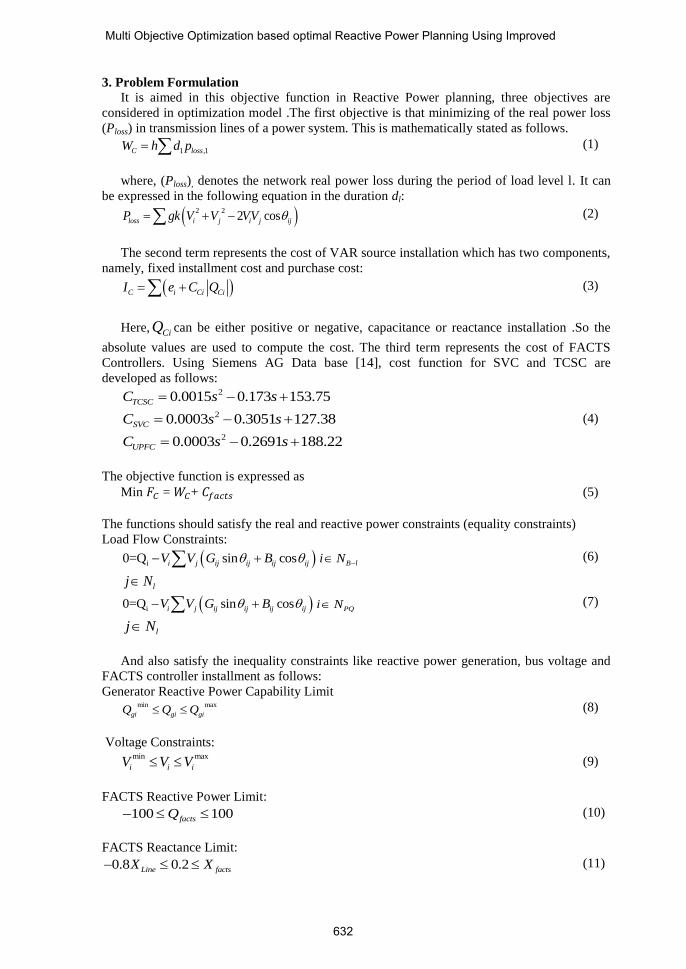
3. Problem Formulation

It is aimed in this objective function in Reactive Power planning, three objectives are

considered in optimization model .The first objective is that minimizing of the real power loss

(Ploss) in transmission lines of a power system. This is mathematically stated as follows.

1 ,1C lossW h d p (1)

where, (Ploss), denotes the network real power loss during the period of load level l. It can

be expressed in the following equation in the duration dl:

2 22 cosloss i j i j ijP gk V V VV (2)

The second term represents the cost of VAR source installation which has two components,

namely, fixed installment cost and purchase cost:

C i Ci CiI e C Q (3)

Here, CiQ can be either positive or negative, capacitance or reactance installation .So the

absolute values are used to compute the cost. The third term represents the cost of FACTS

Controllers. Using Siemens AG Data base [14], cost function for SVC and TCSC are

developed as follows:

20.0015 0.173 153.75TCSCC s s

20.0003 0.3051 127.38SVCC s s (4)

20.0003 0.2691 188.22UPFCC s s

The objective function is expressed as

Min 𝐹𝐶 = 𝑊𝐶+ 𝐶𝑓𝑎𝑐𝑡𝑠 (5)

The functions should satisfy the real and reactive power constraints (equality constraints)

Load Flow Constraints:

i0=Q sin cosi j ij ij ij ijV V G B B li N (6)

lj N

i0=Q sin cosi j ij ij ij ijV V G B PQi N (7)

lj N

And also satisfy the inequality constraints like reactive power generation, bus voltage and

FACTS controller installment as follows:

Generator Reactive Power Capability Limit

min max

gi gi giQ Q Q (8)

Voltage Constraints:

min max

i i iV V V (9)

FACTS Reactive Power Limit:

100 100factsQ (10)

FACTS Reactance Limit:

0.8 0.2Line factsX X (11)

Multi Objective Optimization based optimal Reactive Power Planning Using Improved

632

Q facts can be fewer than zero and if Q facts is chosen as a negative value, say in the light load

period, variable inductive reactive power should be injected at bus i by the FACTS controllers.

Q facts act as a control variable. The load bus voltages Vload and reactive power generations Qg

are state variables, which are limited by adding them as the quadratic penalty terms to the

objective function. Equation (5) is therefore changed to the following generalized objective

function

Min 2 2

lim lim

C C i i gi giF F V V Q Q (12)

limOgi N limVi N

Subjected to

i0=P cos sini j ij ij ij ijV V G B B li N

lj N

i0=Q sin cosi j ij ij ij ijV V G B PQi N

lj N

where, α and β are the penalty factors which can be increased in the optimization procedure; lim

iV and lim

giQ are defined in the following equations:

min min

lim

max

i i i

i max

i i i

V if V VV

V if V V

(13)

min min min

lim

max max max

gi gi gi

gi

gi gi gi

Q if QQ

Q if Q

Q

Q

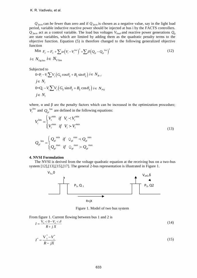
4. NVSI Formulation

The NVSI is derived from the voltage quadratic equation at the receiving bus on a two-bus

system [12],[13],[15],[17]. The general 2-bus representation is illustrated in Figure 1.

Figure 1. Model of two bus system

From figure 1. Current flowing between bus 1 and 2 is

2 2V 0 VI

R j X

(14)

2

* *

1*V V

IR jX

(15)

P1, Q 1 P2, Q2

R+jX

V10ے V2ےδ


633

Comparatively resistance of transmission line is negligible. This equation may be rewritten as

2

* *

1*V V

IjX

(16)

And the receiving end power

2S V I (17)

Incorporating in equation (17) in and solving

1 22 sin

V VP

X (18)

2

1 222 sin

V VVQ

X X (19)

Eliminating 𝜹 from equations yields

2 2 2 2 2 2 2

2 2 1 2 2 2( ) (2 ) ( ) 0V Q X V V X P Q (20)

This is an equation of order of two V2.This condition have at least one solution is

2 2 2 2

2 1 2 2(2 ) 4 ( ) 0Q X V X P Q (21)

2 2

2 2

2

2 1

2 ( )1

2

X P Q

Q X V

(22)

Taking suffix “i” as the sending bus and “j” as the receiving bus, NVSI can be defined by

2 2

2

2 ( )

2

j j

ij

j i

X P QNVSI

Q X V

(23)

Variable definition follows

Z = Line Impedance

X = Line Reactance

Qj = Reactive power at the receiving end

Vi = sending end voltage

θ = line impedance angle

𝜹 = angle difference between the supply voltage and receiving voltage

Pi = sending end real power

A. Determining the maximum load-ability for Weak Bus Identification

The following steps are implemented:

Step 1: Run the load flow program for the base case.

Step 2: Evaluate the NVSI value for every line in the system.

Step 3: Gradually increase the reactive power loading by 0.01pu at a chosen load bus until

the load flow solution fails to give results for the maximum computable NVSI.

Step 4: Extract the stability index that has the highest value.

Step 5: Choose another load bus and repeat steps 3 and 4.

Step 6: Extract the maximum reactive power loading for the maximum computable NVSI

for every load bus. The maximum reactive power loading is referred to as the

maximum load-ability of a particular bus.


634

Step 7: Sort the maximum load-ability obtained from step 6 in ascending order. The

smallest maximum load-ability is ranked the highest, implying the weakest bus in

the system.

Step 8: Select the weak buses as the FACT controller’s installation site for the RPP

Problem.

5. IEEE 30 Bus system Simulation results have been obtained by using MATLAB 7.5 (R2007b) software package

on a 2.93 GHz, Intel® Core™2 Duo Processor. IEEE 30-bus system [3] has been used to show

the effectiveness of the algorithm. The network consists of 6 generator-buses, 21 load-buses

and 41 branches, of which four branches, (6- 9), (6- 10), (4- 12) and (27-28) are under load-tap

setting transformer branches. The buses for possible VAR source installation based on max

load buses are 25, 26, 29 and 30. The maximum load ability and FVSI values for the IEEE 30

bus system are given in table 1.

Table 1. Bus Ranking and NVSI Values Rank Bus Qmax(p.u) NVSI

1 30 0.27 1.032

2 26 0.32 1.180

3 29 0.35 1.049

4 25 0.50 1.010

5 15 0.54 1.001

6 27 0.60 1.003

7 10 0.65 1.017

8 24 0.69 1.007

9 14 0.78 1.011

10 18 0.79 1.015

The parameters and variable limits are listed in Tables 2 and 3. All power and voltage

quantities are per-unit values and the base power is used to compute the energy cost.

Table 2. Parameters

SB (MVA) h ($/puWh) ei($) Cci ($/puVAR)

100 6000 1000 30,00,000

Table 3. Limits

Qc Vg V load Tg

min max min max min max min max

- 0.12 0.35 0.9 1.1 0.96 1.05 0.96 1.05

Three cases have been studied. Case 1 is of light loads whose loads are the same as those in

[3]. Case 2 and 3 are of heavy loads whose loads are 1.25% and 1.5% as those of Case 1. The

duration of the load level is 8760 hours in both cases [6].

Initial Power Flow Results

The initial generator bus voltages and transformer taps are set to 1.0 pu. The loads are given as,


635

Case 1: Pload = 2.834 and Qload = 1.262

Case 2: Ploa d= 3.5425 and Qload = 1.5775

Case 3: Pload = 4.251 and Qload = 1.893

Table 4. Initial generations and power losses

Pg Qg Ploss Qloss

Case 1 3.008 1.354 0.176 0.323

Case 2 3.840 2.192 0.314 0.854

Case 3 4.721 3.153 0.461 1.498

Table 5.Optimal generator bus voltages.

Bus 1 2 5 8 11 13

Case 1 1.10 1.09 1.05 1.09 1.10 1.10

Case 2 1.10 1.10 1.09 1.10 1.10 1.10

Case 3 1.10 1.10 1.08 1.09 1.09 1.09

Table 6.Optimal transformer tap settings.

Branch (6-9) (6-10) (4-12) (27=28)

Case 1 1.0433 0.9540 1.0118 0.9627

Case 2 1.0133 0.9460 0.9872 0.9862

Case 3 1.0131 0.9534 0.9737 0.9712

Table 7. Optimalvar source installments.

Bus 26 28 29 30

Case 1 0 0 0 0

Case 2 0.0527 0.030 0.022 0.031

Case 3 0.0876 0.029 0.027 0.047

Table 8.Optimal generations and power losses Using NIDE

Pg Qg Ploss Qloss

Case 1 2.989 1.288 0.159 0.266

Case 2 3.808 1.867 0.266 0.652

Case 3 4.659 2.657 0.417 1.190

The optimal generator bus voltages, transformer tap settings, VAR source installments,

generations and power losses are obtained as in Tables V - VIII.Form Table VIII,the active

power losse is considerably reduced for case 1 from 0.176 to 0.159 using NIDE.

The real power savings, annual cost savings and the total costs are calculated as,

𝑃𝐶𝑆𝑎𝑣𝑒% =

𝑃𝑙𝑜𝑠𝑠𝑖𝑛𝑡 −𝑃𝑙𝑜𝑠𝑠

𝑜𝑝𝑡

𝑃𝑙𝑜𝑠𝑠𝑖𝑛𝑡 x 100 % (24)

𝑊𝐶𝑠𝑎𝑣𝑒 = hdl ( 𝑃𝑙𝑜𝑠𝑠

𝑖𝑛𝑡 − 𝑃𝑙𝑜𝑠𝑠𝑜𝑝𝑡

)


636

Table 9. Comparison Results

Variables Case-1 Case-3

EP NIDE EP NIDE

V1 1.05 1.05 1.05 1.05

V2 1.044 1.044 1.022 1.022

T6-9 1.05 1.0433 0.9 1.013

T4-12 0.975 1.031 0.95 0.973

QC 17 0 0 0.0229 0.297

QC 27 0 0 0.196 0.297

PG 2.866 2.989 5.901 4.659

QG 0.926 1.288 2.204 2.657

Ploss 0.052 0.159 0.233 0.417

Qloss 0.036 0.266 0.436 1.190

As shown in Table Similar results were obtained both approaches for the Case-1 and Case-

2 NI DE adjusted the voltage magnitude of all PV buses and transformer tap settings such that

total losses decreased.

6. Modeling of FACTS Controllers

SVC, TCSC and UPFC mathematical models are implemented by MATLAB programming.

Steady state model of FACTS controllers in this paper are used for power flow studies .

A. TCSC

TCSC, the first generation of FACTS, can control the line impedance through the

introduction of a thyristor controlled capacitor in series with the transmission line. A TCSC is a

series controlled capacitive reactance that can provide continuous control of power on the ac

line over a wide range. In this paper, TCSC is modeled by changing the transmission line

reactance as below

cscij line rX X X (25)

where, Xline is the reactance of transmission line and XTCSC is the reactance of TCSC. Rating of

TCSC depends on transmission line where it is located. To prevent overcompensation, TCSC

reactance is chosen between -0.8Xline to 0.2 Xline.

B. SVC

SVC can be used for both inductive and capacitive compensation. In this work SVC is

modeled as an ideal reactive power injection controller at bus i

i SVCQ Q (26)

C. UPFC

The decoupled model of UPFC is used to provide independent shunt and series reactive

compensation. The shunt converter operates as a standalone STATIC synchronous

Compensator (STATCOM) and the series converter as a standalone Static Synchronous Series

Compensator (SSSC). This feature is included in the UPFC structure to handle contingencies

(e.g., one converter failure). In the stand alone mode, both the converters are capable of

absorbing or generating real power and the reactive power output can be set to an arbitrary

value depending on the rating of UPFC to maintain bus voltage.

7. New Improved Differential Evolution (NIDE)

Differential Evolution was first proposed over 1994-1996 by Storn and Price at

Berkeley.DE is a mathematical global optimization method for solving multi-dimensional

functions. The main idea of DE is to generate trial parameter vectors using vector differences

for perturbing the vector population.


637

In order to improve the performance of differential evolution, the proposed novel

algorithm which will generate a dynamical function for changing the differential evolution

parameter mutation factor replace traditional differential algorithm use constant mutation

factor.

A. Main Steps of the NIDE Algorithm

The working procedure algorithm is outlined below:

Initialize the population set uniformly

Sort the population set S in ascending order

Partition S into p sub populations S1,S

2,…..,S

P each containing m points, such that

1

, : 1,......,k k kk

J j J k p jS X f X X j m

1,............,K p

Apply improved DE algorithm to each sub population S

k to maximum number of

generation Gmax Replace the sub populations S

1,S

2,…S

p and check whether the termination

criterion met if yes then stop otherwise go to step 2

Using, Selection, Cross over Factor, Mutation Factor and Recombination are Calculated.

B. New Improved Differential evolution for OPF using TCSC

Step 1: Parent vectors of size NP are randomly generated. Elements in a parent vector

are real power generation of the generating units excluding slack bus, voltage

magnitude and phase angle of the buses excluding slack bus and series capacitors of Thyristor Controlled Switched Capacitor. The𝑖𝑡ℎ parent vector is as follows:

𝑃𝑖 = [𝑃𝐺1𝑖 … . . 𝑃𝐺𝑚

𝑖 … . 𝑃𝐺𝑛𝑖 , 𝑉1…

𝑖 𝑉𝑛𝑖 … 𝛿1

𝑖 … . . 𝛿𝑚𝑖 … 𝑋𝑇𝐶𝑆𝐶1

𝑖 … . . 𝑋𝑇𝐶𝑆𝐶𝑛𝑖 ]T

The reactive power generations, transmission loss, slack bus generations and

line flows are calculated. Cost of generation is calculated for each parent

vector pi.

Step 2: Perform mutation for each target vector as described in Section 4.2

Step 3: Perform crossover for each target vector and create a trial vector as mentioned

in Section 4.3.

Step 4: Perform selection for each target vector, by comparing its cost with that of the

trial vector. The vector that has lesser cost of the two would survive for the

next generation.

Step 5: Stop if the maximum number of generations is reached otherwise go to Step 2

8. Case Study Table 10. Comparison Results

Variables Case-1 Case-3

IDE EP IDE EP

V1 1.05 1.05 1.05 1.05

V2 1.044 1.044 1.022 1.022

T6-9 1.05 1.0433 0.9 1.013

T4-12 0.975 1.031 0.95 0.973

QC 17 0 0 0.0229 0.297

QC 27 0 0 0.196 0.297

PG 2.866 2.989 5.901 4.659

QG 0.926 1.288 2.204 2.657

Ploss 0.052 0.159 0.233 0.417

Qloss 0.036 0.266 0.436 1.190


638

A simplified Indian 400- kV transmission network with 72 buses (55 PV buses and 15 PQ

buses) and is used for testing. One line diagram is shown in figure 2. FACTS locations are

identified based on the FVSI technique. The greatest load ability and FVSI values for the real

time system are given in Table 10.

Table 11. Bus Ranking and FVSI Values Rank Bus Qmax(p.u) NVSI

1 25 0.23 0.9837

2 27 0.27 0.9841

3 56 0.28 0.9964

4 52 0.35 0.9925

5 45 0.43 0.9843

6 59 0.45 0.9932

7 37 0.47 0.9972

8 46 0.48 0.9887

9 68 0.56 0.9863

10 64 0.57 0.9897

11 30 0.59 0.9852

12 29 0.63 0.9922

13 36 0.658 0.9787

14 49 0.67 0.9858

15 55 0.71 0.9871

16 19 0.712 0.9936

17 17 0.732 0.997

18 53 0.74 0.9856

19 16 0.77 0.9879

20 61 0.81 0.9989

21 18 0.85 0.9947

22 57 0.856 0.9937

23 26 0.87 0.9859

24 23 0.881 0.9986

25 33 0.893 0.9783

26 48 0.9 0.9949

27 34 0.911 0.9929

28 59 0.925 0.9893

29 51 0.96 0.9801

30 40 0.962 0.9857

31 42 0.982 0.9862

32 38 0.988 0.9999

33 22 0.99 0.9931

34 43 1.01 0.9976

35 19 1.1 0.9798

36 32 1.13 0.998

37 18 1.19 0.9879

38 41 1.22 0.9899

39 52 1.27 0.9871

40 45 1.3 0.9759

41 54 1.34 0.9795

42 28 1.354 0.9889

43 26 1.378 0.9567

44 60 1.39 0.9854

45 21 1.415 0.9912

46 59 1.42 0.9877

47 44 1.47 0.9945

48 47 1.51 0.9947

49 50 1.54 0.9858

50 20 1.59 0.9857

51 31 1.61 0.9982

52 36 1.75 0.9865

53 32 1.61 0.9789

54 39 1.88 0.9658

55 69 1.93 0.9687

56 66 1.98 0.9723

57 46 2.03 0.9834


639

The proposed method compares the effectiveness of Evolutionary Programming (EP), and

Improved Differential Evolution (IDE) to solve reactive power planning problem incorporating

FACTS controllers Like TCSC, SVC and UPFC considering voltage stability, with help of Fast

Voltage Stability Index (FVSI).The critical lines and buses are identified to install the FACT

controllers.

As shown in Table 11 in both approaches for the case 1 and case 3 using IDE adjusted the

voltage magnitude of all PV buses and transformer tap settings such that total real and reactive

power losses decreased as comparing with EP.

Figure 2. Indian network.

From Table 11, bus 25 has the smallest maximum load-ability implying the critical bus and

branch 26-28 has the maximum FVSI close to one indicates the critical line referred to bus 38.

Hence, SVC is installed at bus 25, TCSC is installed in the branch 26-38. UPFC is installed at

midpoint of branch 26-38.Two cases have been studied. Case 1.is the light load, case 2 is heavy

loads and whose load is 125%.

Table 13. Optimal Generator Bus Voltages

BUS Case 1 Case 2

SVC TCSC UPFC SVC TCSC UPFC

1 1.0999 1.0999 1.0999 1.0999 1.0999 1.0999

12 1.0859 1.0876 1.0821 1.0994 1.0982 1.0977

15 1.0951 1.0924 1.0857 1.0999 1.0988 1.0884

24 1.0994 1.0897 1.0791 1.0996 1.0874 1.0741

35 1.0854 1.0796 1.0774 1.0802 1.0784 1.0721

FACTS device settings, optimal generator bus voltages and optimal generation and power

losses are obtained as in Table 13 to 15.

Table 14. FACTS Device Settings

Parameters FACTS Location Case 1 Case2

X TCSC 26-28 -0.1672 -0.08006

Qsvc Bus 30 0.2 0.2

QUPFC 26-28 0.1974 0.29421

QUPFC 26-28 -0.0432 -0.06732


640

Table 15. Optimal Generations and Power losses

Pg(MW) Qg(MVAR) Ploss(MW) Qloss(MVAR)

Case 1

SVC 30.017 10.994 0.1655 0.3054

TCSC 29.895 13.678 0.1642 0.2849

UPFC 29.876 11.644 0.1639 0.2651

Case 2

SVC 38.965 18.159 0.2976 0.7781

TCSC 38.724 18.043 0.2835 0.7054

UPFC 38.701 17.975 0.2687 0.6827

Table 16. Performance Comparison

Loading FACT

Devices

USING EP USING IDE

PCsave % WC Save ($) PCsave % WC Save ($)

Case-1

SVC 8.832 8.42× 106 9.182 8.67× 106

TCSC 9.507 9.07×106 9.807 9.19×106

UPFC 9.669 9.22× 106 9.988 9.30 × 106

Case-2

SVC 9.040 1.55× 107 10.04 1.64× 107

TCSC 13.341 2.29×107 14.46 2.37× 107

UPFC 17.851 3.06×107 16.65 3.15× 107

From table 14 the UPFC gives more savings on the real power and annual cost compared to

SVC and TCSC for both cases.

Figure 3. Voltage profile improvement for case 2 using FACT Devices.

Figure 3, illustrated the response for Bus number Vs Bus voltage magnitude. From plot, using

IDE approach for case 2 with FVSI, UPFC controller gives the better voltage magnitude.

9. Conclusion

In this Paper, New Improved Differential Evolution Algorithm is implemented for optimal

reactive power planning problem. The ability of this algorithm has been assessed by testing on

IEEE-30 Bus, Indian utility 72 Bus systems. The obtained results are compared with other


641

method reported in given references. It is concluded that, the obtained results in this paper are

better than the obtained in other reported papers.

10. References [1]. A. Kishore and E.F. Hill, 1971, “Static optimization of reactive power sources by

use of sensitivity parameters,” IEEE Transactions on Power Apparatus and

Systems, PAS-90, pp.1166-1173

[2]. S.S. Sachdeva and R. Billinton, 1973, “Optimum network VAR planning by

nonlinear programming,” IEEE Transactions on Power Apparatus and Systems,

PAS-92, 1217 – 1225

[3]. K.Y.Lee, Y.M.Park and J.L.Ortiz, 1985, “A united approach to optimal real and

reactive power dispatch,” IEEE Transactions on Power Apparatus an

Systems,Vol. PAS-104, No.5, pp.1147– 1153

[4]. Kenji Iba, 1994, “Reactive Power Optimization by Genetic Algorithm,” IEEE

Transactions on Power Systems, Vol. 9, No, 2, pp. 685 – 692.

[5]. L.L.Lai and J.T.Ma, 1997, “Application of Evolutionary Programming to

Reactive Power Planning Comparison with nonlinear programming approach,”

IEEE Transactions on Power Systems, Vol. 12, No.1, pp. 198 – 206

[6]. Wenjuan Zhang, Fangxing Li, Leon M. Tolbert, 2007, “Review of Reactive

Power Planning: Objectives, Constraints, and algorithms,” IEEE Transactions on

Power Systems, Vol. 22, No. 4.

[7]. P.J.Angeline, 1995, “Evolution revolution: an introduction to the special track on

genetic and evolutionary programming,” IEEE Expert, 10, pp. 6 – 10

[8]. Kalyanmoy Deb, 2001, “Multi-Objective Optimization using Evolutionary

Algorithms,” John Wiley and Sons Ltd.

[9]. M. Noroozian, L. Angquist, M. Ghandhari, G. Anderson, 1997, “Improving

Power System Dynamics by Series-connected FACTS Devices,” IEEE

Transaction on Power Delivery, Vol. 12, No.4.

[10]. M. Noroozian, L. Angquist, M. Ghandhari, 1997, “Use of UPFC for Optimal

Power Flow Control,” IEEE Trans. on Power Delivery, Vo1.12, No.

[11]. N.G. Hingorani, L. Gyugyi, 2000, “Understanding FACTS: Concepts and

Technology of Flexible AC Transmission Systems,” IEEE Press, New York

[12]. S.N. Sing, A.K. David, 2001, “A New Approach for Placement of FACTS

Devices in Open Power Markets”, IEEE Power Engineering Review, Vol. 21,

No.9, 58 - 60.

[13]. D. Thukaram, L. Jenkins, K. Visakha, 2005, “Improvement of system security

with Unified Power Flow Controller at suitable locations under network

contingencies of interconnected systems,” IEEE Trans. on Generation,

Transmission and Distribution, Vol. 152, Issue 5, pp. 682

[14]. www.siemens/td.com/trans.Sys/pdf/cost/EffectiveRelibTrans.pdf

[15]. M. Moghavemmi and F.M. Omar, 1998, “Technique for contingency monitoring

and voltage collapse prediction,” IEE Proc. Generation, Transm and

Distribution, vol. 145, pp. 634-640

[16]. A.C.G. Melo, S. Granville, J.C.O. Mello, A.M. Oliveira, C.R.R. Dornellas, and

J.O. Soto, 1999, “Assessment of maximum loadability in a probabilistic

framework,” IEEE Power Eng. Soc.Winter Meeting, vol. 1, pp. 263-268

[17]. I.Musirin,and T.K.A.Rahman, “Estimating Maximum Loadabilty for Weak Bus

using Fast Voltage Stability Index”, IEEE Power Engineering review, pp.50-52,

2002


642

[18]. Guang Ya Yang ,Zhao yang Dong, “A Modified Differential Evolution

Algortihm with Fitness Sharing for power system planning,” IEEE Tranaction on

power Engineering,Vol.23, pp.514-552,2012

[19]. Lonescu, C.F.Bulac.C, “Evolutionary Techniues,a sensitivity based approach for

handling discrete variables in Reactive Power Planning,” IEEE Tansaction on

Power Engineering, pp.476-480,2012

[20]. Vaahedi, Y. Mansour, C. Fuches, “Dynamic security Constrained optimal power

flow/Var Planning,” IEEE Transaction in power systems,Vol.16.pp.38-43,2001

[21]. R.Kanimozhi and K. Selvi, A Novel Line Stabilty Index for Voltage Stability

Analysis and ContigencyRanking in Power Systems using Fuzzy Based Load

Flow, J.Electrical Engineering Technolology Vol.8, No.4.pp.694-703,2013.

K. R. Vadivelu received the B.E.Electrical and Electronics Degree from

Bharathiyar University, Coimbatore in 1997 and the M.Tech Degree in Power

Systems from SASTRA University Tanjore, Tamilnadu in 2006 and pursuing

Ph.D. in Electrical and Electronics Engineering at S.V.University College of

Engineering, S.V.University, Tirupati, Andhra Pradesh. Currently he is

working as a Professor in Electrical and Electronics Engineering department

at Sree Venkateswara College of Engineering and Technology, Chittoor,

Andhra Pradesh, India.

G. Venkata Marutheswar received B.Tech Degree in Electrical

Engineering, the M.Tech (with Distinction) Degree in Instrumentation and

Control Engineering and Ph.D Degree in Electrical and Electronics

Engineering from Sri Venkateswara University College of Engineering,

S.V.University, Tirupati, Andhra Pradesh in 1985,1990 and

2009,respectively.Currently,he is Working as a Professor in the department of

Electrical and Electronics Enginering, S.V.University College of

Engineering,Tirupati, Andhra Pradesh, India.


643

multi objective optimization based optimal reactive …ijeei.org/docs-8104997515684fb1d2e58d.pdf ·...

Documents