Multiple Unstructured Meshes andthe design of freefem+ ∗

F. Hecht†& O. Pironneau‡

December 27, 1998

AbstractProblems involving partial differential equations (pde) of several

branches of physics such as fluid-structure interactions require inter-polations of data on several meshes and their manipulation within oneprogram. In this report we build on a fast quadtree-based interpola-tion algorithm, propose a language for the manipulation of data onmultiple meshes and test by designing an extension of freefem[1]. Fi-nally we present 3 applications: a mesh refinement for a problem witha singularity, the new Schwarz like domain decomposition method in-troduced in [4] and a fluid-structure interaction problem.

ResumeLorsque les equations aux derivees partielles des problemes a

resoudre impliquent plusieurs branches de la physique, commepar exemple les interactions fluides-structures, on doit manipulernumeriquement plusieurs maillages dans un meme programme et in-terpoler les donnees d’un maillage sur un autre. Dans ce rapport nouspresentons un interpoleur rapide construit sur un quadtree, nous pro-posons un language de manipulation de triangulations et de donneeset nous illustrons ces notions par une extension de freefem [1] et sur3 applications: un probleme de maillage adaptatif pour la resolutiond’une singularite, la nouvelle methode de decomposition de domainepresentee dans [4] et un probleme d’interaction fluide-structure.

∗ftp://ftp.ann.jussieu.fr/pub/soft/pironneau†Frederic.Hecht@inria.fr‡Olivier.Pironneau@ann.jussieu.fr

1

Contents

1 Introduction 4

2 Examples and problem statements 42.1 A corner singularity . . . . . . . . . . . . . . . . . . . 52.2 Domain Decomposition . . . . . . . . . . . . . . . . . 5

2.2.1 Extension . . . . . . . . . . . . . . . . . . . . . 72.3 Fluid-Structure interactions . . . . . . . . . . . . . . . 8

3 A Fast Finite Element Interpolator 93.1 Algorithm . . . . . . . . . . . . . . . . . . . . . . . . 93.2 Remark . . . . . . . . . . . . . . . . . . . . . . . . . . 11

4 Mesh Adaption 11

5 The Design of Freefem+ 125.1 Reserved words . . . . . . . . . . . . . . . . . . . . . . 12

5.1.1 Commands . . . . . . . . . . . . . . . . . . . . 125.1.2 Reserved variables . . . . . . . . . . . . . . . . 13

5.2 Transparent Interpolator . . . . . . . . . . . . . . . . . 135.3 Meshes . . . . . . . . . . . . . . . . . . . . . . . . . . 14

5.3.1 Example 1: the mesh for the corner singularity 155.3.2 Example 2: meshs for domain decompositions . 155.3.3 Example 3: meshes for fluid-structure interaction 15

5.4 Data Types . . . . . . . . . . . . . . . . . . . . . . . . 165.5 Expressions . . . . . . . . . . . . . . . . . . . . . . . . 17

5.5.1 int . . . . . . . . . . . . . . . . . . . . . . . . . 175.6 Partial Differential Equations . . . . . . . . . . . . . . 19

5.6.1 Solve . . . . . . . . . . . . . . . . . . . . . . . . 195.6.2 varsolve . . . . . . . . . . . . . . . . . . . . . . 195.6.3 The domain decomposition algorithms . . . . . 195.6.4 Implementation strategy . . . . . . . . . . . . . 215.6.5 Fluid-Structure . . . . . . . . . . . . . . . . . . 22

5.7 Mesh adaption with ”adaptmesh” . . . . . . . . . . . . 245.7.1 The corner singularity problem . . . . . . . . . 24

6 Appendix A: Details on the syntax of freefeem+ 266.1 Syntax of int . . . . . . . . . . . . . . . . . . . . . . . 266.2 Syntax of ”solve” . . . . . . . . . . . . . . . . . . . . . 26

2

6.3 Syntax of ”on” within solve . . . . . . . . . . . . . . . 276.4 Syntax of ”varsolve” . . . . . . . . . . . . . . . . . . . 286.5 Syntax of ”convect” . . . . . . . . . . . . . . . . . . . 286.6 Other keywords . . . . . . . . . . . . . . . . . . . . . . 29

7 Appendix B: Line output offreefem+ for Example 1 (Schwarz algorithm) 30

NOTE freefem 3.4 is available athttp://www.asci.fr

freefem+ v0.9.31 is available at

ftp://ftp.ann.jussieu.fr/pub/soft/pironneau

with the source C++ code and a graphic interface for the Mac, PC,HP-UX and Linux. It compiles with CodeWarrior pro 4 and gnu C++2.8 or later.

3

1 Introduction

Many problems involve several equations of physics. fluid-structureinteractions, Lorenz forces in liquid aluminium and ocean-atmosphereproblems are three such systems. Some algorithms such as Schwarz’domain decomposition method require also the interpolation of dataon different meshes within one program.More recently it was pointed in [4] that the problem of solving pdeswithin the data structures of Virtual Reality (usually CSG, construc-tive Solid Geometry) also requires the manipulation of many mesheswithin one program.Interpolation from one unstructured mesh to another is not easy be-cause it has to be fast and non-diffusive. Furthermore one has to findfor each point the triangle which contains it and that is one of the ba-sic problem of computational geometry (see Preparata & Shamos[6]for example). To do it in the minumum number of operations is thechallenge.We propose here an implementation which is O(n logn) based on aquadtree. The algorithm is rather straightforward and the value ofthis report is more on the implementation made and on the report ofits performance.Our purpose is also to investigate methods which relieve the user fromthe programming burden of interpolation on multiple meshes. For thiswe use the program freefem[1] redesigned it completely in C++ withtemplates and extended it to multiple meshes. The outcome is a ver-satile software for the above mention problems: freefem+.To illustrate our purpose we will apply it to fluid-structure interactionsand to a new type of Schwarz algorithm for domain decompositionpresented in[4] and which we recall below.

2 Examples and problem statements

Freefem+ was developped to solve problems which involve more thanone mesh for their discretization. To illustrate this we propose 3 ex-amples: the resolution of a corner singularity,a domain decompositionalgorithm similar to Schwarz algorithm and a fluid-structure interac-tion problem.

4

2.1 A corner singularity

The domain is an L-shaped polygon and the pde is

Find u ∈ H10 (Ω) such that −∆u = f in Ω,

The solution has a singularity at the reentrant angle and we wishto capture it numerically. In our example f = 1 and the domainboundary is the polygon of vertices (0, 0) (0, 1) (1, 1

2) (12 ,

12) (1

2 , 1) (0, 1)

2.2 Domain Decomposition

We wish to solve the same Laplace equation in Ω when

Ω = Ω1 ∪ Ω2 such that Ω12 = Ω1 ∩ Ω2 6= 0.

which, in variational form is∫Ω∇u · ∇v =

∫Ωfv, ∀v ∈ V = H1

0 (Ω)

Schwarz’ domain decomposition algorithm can be used here.

Algorithm 1

Begin loop

• Compute um+11 by solving

−∆um+11 = f in Ω1, um+1

1 = um2 on S1 = ∂Ω12 ∩ Ω2

• Compute um+12 by solving

−∆um+12 = f in Ω2, um+1

2 = um+11 on S2 = ∂Ω12 ∩ Ω1

End loopIn our example f = 1, Ω1 is the rectangle (0, 2)× (0, 1) and Ω2 is

the unit circle.

5

Algorithm 2

Algorithm 2 is an alternative which does not require an interpolationon boundaries but in the interior of the domains.

Let

Vi = v ∈ L2(Ω) : v|Ωi ∈ H10 (Ωi), v|Ω\Ωi = 0

Choose ρ > 0.Begin loop

• Compute un+11 ∈ V1 such that∫

Ω1∩Ω2

ρ(un+11 −un1 )v1+

∫Ω∇(un+1

1 +un2 )·∇v1 =∫

Ωfv1, ∀v1 ∈ V1.

• Compute un+12 ∈ V2 such that∫

Ω1∩Ω2

ρ(un+12 −un2 )v2+

∫Ω∇(un1 +un+1

2 )·∇v2 =∫

Ωfv2, ∀v2 ∈ V2

End loopIt is in fact a variation of Schwarz algorithm because if we callvn+1

1 = un+11 + un2 , vn+1

2 = un+12 + un1 we find that these verify a

time dependant version of Algorithm 1. However the convergence iseasier to show and the discretization is different. The convergence ofthis algorithm is given by the following result

Theorem 1(J.L.Lions[4])Algorithm 1 converges in the sense that uni → u∗i with u∗1 + u∗2 = usolution of (1) and the decomposition is uniquely defined by

(B +A)u1 =12

(B +A)(u+ u01 − u0

2) in Ω12, u1|S1 = 0, u1|S2 = u

(B +A)u2 =12

(B +A)(u+ u02 − u0

1) in Ω12 u2|S2 = 0, u2|S1 = u

6

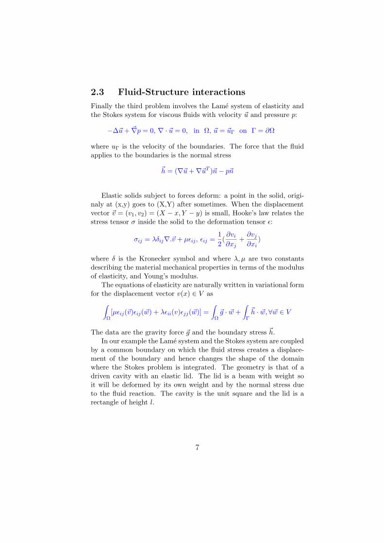
2.3 Fluid-Structure interactions

Finally the third problem involves the Lame system of elasticity andthe Stokes system for viscous fluids with velocity ~u and pressure p:

−∆~u+ ~∇p = 0, ∇ · ~u = 0, in Ω, ~u = ~uΓ on Γ = ∂Ω

where uΓ is the velocity of the boundaries. The force that the fluidapplies to the boundaries is the normal stress

~h = (∇~u+∇~uT )~n− p~n

Elastic solids subject to forces deform: a point in the solid, origi-naly at (x,y) goes to (X,Y) after sometimes. When the displacementvector ~v = (v1, v2) = (X − x, Y − y) is small, Hooke’s law relates thestress tensor σ inside the solid to the deformation tensor ε:

σij = λδij∇.~v + µεij , εij =12

(∂vi∂xj

+∂vj∂xi

)

where δ is the Kronecker symbol and where λ, µ are two constantsdescribing the material mechanical properties in terms of the modulusof elasticity, and Young’s modulus.

The equations of elasticity are naturally written in variational formfor the displacement vector v(x) ∈ V as∫

Ω[µεij(~v)εij(~w) + λεii(v)εjj(~w)] =

∫Ω~g · ~w +

∫Γ

~h · ~w, ∀~w ∈ V

The data are the gravity force ~g and the boundary stress ~h.In our example the Lame system and the Stokes system are coupled

by a common boundary on which the fluid stress creates a displace-ment of the boundary and hence changes the shape of the domainwhere the Stokes problem is integrated. The geometry is that of adriven cavity with an elastic lid. The lid is a beam with weight soit will be deformed by its own weight and by the normal stress dueto the fluid reaction. The cavity is the unit square and the lid is arectangle of height l.

7

3 A Fast Finite Element Interpolator

In the last two examples above there are two domains Ωi, i = 1, 2. Inpractice one may discretize the pdes by the Finite Element method.Then there will be one mesh for Ω1 and another one for Ω2 and mixedintegrals of product of functions defined on both meshes.The computation of integrals of products of functions defined on differ-ent meshes is difficult. Quadrature formulae and interpolations fromone mesh to another at quadrature points are needed. We present be-low an interpolation operator first for two meshes of the same domain,then for two meshes of two different domains.

Let T 0h = ∪kT 0

k , T 1h = ∪kT 1

k be 2 triangular meshes of Ω. Let

V (T ih) = C0(Ωih) : f |T i

k∈ P 1, i = 0, 1

be the spaces of continuous piecewise affine functions on each mesh.Let f ∈ V (T 0

h). The problem is to find g ∈ V (T 1h) such that

g(q) = f(q) ∀q vertex of T 1h

Although this is a seemingly simple problem, it is difficult to find anefficient algorithm in practice. We propose an algorithm which is ofcomplexity N1 logN0, where N i is the number of vertices of T ih, andwhich is very fast for most practical 2D applications.In practice even though the initial domain Ω is the same, the discretedomains are different, so important decisions must be made if q isinside T 0

h but outside T 1h. This choice also governs the case when

T 0h, T 1

h are triangulations of Ω0 6= Ω1.

DefinitionIf q is inside T 0

h but outside T 1h we define the interpolate by

g(q) = f(q⊥)

where q⊥ is the projection of q on the boundary of Ω0.

3.1 Algorithm

The method has 5 steps. First a quadtree is built containing all thevertices of mesh T 0

h such that in each terminal cell there are at leastone, and at most 4, vertices of T 0

h .For each q1, vertex of T 1

h do:

8

q1

q0

Tk0

• Step 1 Find the terminal cell of the quadtree containing q1.• Step 2 Find the the nearest vertex q0

j to q1 in that cell.

• Step 3 Choose one triangle T 0k ∈ T 0

h which has q0j for vertex.

• Step 4 Compute the barycentric coordinates λjj=1,2,3 of q1 inT 0k .– if all barycentric coordinates are positive, go to Step 5– else if one barycentric coordinate λi is negative replace T 0

k

by the adjacent triangle opposite q0i and go to Step 4.

– else two barycentric coordinates are negative so take one ofthe two randomly and replace T 0

k by the adjacent triangleas above.

• Step 5 Calculate g(q1) on T 0k by linear interpolation of f :

g(q1) =∑

j=1,2,3

λjf(q0j )

• End

Two problems needs to be solved:

• What if q1 is not in Ω0h ? Then Step 5 will stop with a boundary

triangle. So we add a step which test the distance of q1 with thetwo adjacent boundary edges and select the nearest, and so ontill the distance grows.

• What if Ω0h is not convex and the marching process of Step 4

locks on a boundary? By construction Delaunay-Voronoi meshgenerators always triangulate the convex hull of the vertices ofthe domain. So we make sure that this information is not lostwhen T 0

h, T 1h are constructed and we keep the triangles which

are outside the domain in a special list. Hence in step 5 we canuse that list to step over holes if needed.

9

Figure 0. To interpolate a function at q0 the knowledge of the trianglewhich contains q0 is needed. The algorithm may start at q1 ∈ T 0

k andstall on the boundary (thick line) because the line q0q1 is not insideΩ. But if the holes are triangulated too (doted line) then the problemdoes not arise.

Remark Step 3 requires an array of pointers such that each vertexpoints to one triangle of the triangulation.

4 Mesh Adaption

Mesh adaption is an important asset of unstructured mesh solvers. In[3] an adaptive procedure is presented, based on a change of metric inthe Delaunay - Voronoi algorithm.

The idea is that the error of interpolation on a mesh is boundedby

‖u− uh‖ < C‖∇(∇u))‖h2

Therefore an attempt to keep ~hT∇(∇u)~h constant could pay. If severalfunctions are specified as for the mesh adaption, for instance u andv then it is min~hT∇(∇u)h, hT∇(∇v)~h which will be kept constantand equal to ε. More precisely the method is to apply the Delaunay-Voronoi triangulation algorithm with the distance based on these Hes-sians (so that circles become ellipses). It is however substantially morecomplex because a function may have a non positive definite Hessian.

To define a metric the Hessian is diagonalized:

D2u =

(∂2u/∂x2 ∂2u/∂x∂y∂2u/∂x∂y ∂2u/∂y2

)= R

(λ1 00 λ2

)R−1,

where R is the eigenvectors matrix of D2u and λi its eigenvalues. Themetric is defined by xTMy, x, y ∈ R2 with:

M = R(λ1 00 λ2

)R−1, and λi = min(max(

|λi|ε,

1h2max

),1

h2min

),

with hmin and hmax being the minimal and maximal edge lengthsallowed in the mesh and ε the tolerance.

10

If two functions are specified for adaption, then, denoting by λjiand vji , i, j = 1, 2 the eigen-values and eigen-vectors of Mj , j = 1, 2,the intersection metric M is defined by

M =12M1 + M2.

where M1 is the matrix with the same eigenvectors and for eigenval-ues:

λ1i = max(λ1

i , v1iTM2v

1i ), i = 1, 2.

5 The Design of Freefem+

5.1 Reserved words

5.1.1 Commands

A list of commands is given below with short or self explainations

1. " R2 " changes the name of x,y." exit " as in C

2. " if " " then " " else " if-statement" for " " to " " do " do-loop

3. " mesh " " border " " buildmesh " " savemesh "" readmesh " " movemesh " " adaptmesh " mesh commands

4. " function " " number " " array" " femp0 "" plot " " plot3d " " save " " fepmp1 "" read " " print " " append" " plotp0 "

5. " convect " " dx " " dy " " laplace "" dxx " " dxy " " dyx " " dyy " " dnu "

7. " varsolve " " with " " on " " solve " " pde "8 " int " " Id " " assemble " " derive "9 " subroutine "

• ”R2(x,y,ref)” means that the problem is 2D with variable x,y.Borders can be grouped into one unit by assigning to each thesame ”ref”.

• ”exit” is useful for program development.

11

• woX = convect(u,v,dt,w); means that w(x,y) is convected by theflow during a time interval dt: woX(x, y) = w(X,Y ):

dX

dt= u(X,Y ),

dY

dt= v(X,Y ), X(t− δt) = x;Y (t− δt) = y.

• All the operators like dx(u) can be used inside and outside pdes;dnu(u) is not the normal derivative of u by its conormal. (Recallthat the natural Neumann condition for an elliptic operator −∇·(A∇u) involves A~n · ∇u which is also ∂u/∂ν if ~ν = A~n).

• Id(u > 1) is the Heavyside function; it is same as the logicalexpression (u > 1), only more readible.

• ”assemble” and ”derive” are for future uses.

5.1.2 Reserved variables

• ”pi” = 4*atan(1.).

• ”wait”: if wait /∈ (−1, 0) graphics halt the program and themouse must be clicked by the user. The variable wait controlsalso the way plots are displaid and stored (see the section on”plot”).

• ”nrmlx”, ”nrmly”: components of the normal. (=0 if not onboundary)

5.2 Transparent Interpolator

Each piecewise linear function is either user defined or generated in-ternally by freefem+. It is stored as

1. A pointer to the triangulation on which the function is defined.

2. An array of values of the function on each vertex of the triangu-lation.

The basic idea is that with the interpolator the user does not needto know on which triangulation the function has been defined. Atany moment there is an active triangulation and when a value of afunction is needed the interpretor checks if the triangulation pointerof the function points to the active triangulation and if it does not itcalls the interpolator.

12

The default active triangulation is set by ”mesh”which is thekeyword preceeding ”buildmesh”, ”movemesh”, ”adaptmesh” and”readmesh”. All keywords which have a triangulation in their parame-ters change the default active mesh into their local active triangulationwithin the scope of their action.

For instance the display of a function on two meshes is transparentto the user:

mesh mesh1; // makes mesh1 the active default mesh.array(mesh1) u = x^2 + y^2;plot(u); // identical to plot(mesh1,u);plot(mesh2,u);

The first plot command is standard. In the second one the activemesh is mesh2 and since it is different from mesh1 on which u hasbeen defined, the interpolator is called.

5.3 Meshes

A domain is defined as being on the left (resp right) of its orientedboundary if the sign of the expression that returns the number ofvertices on the boundary is positive (resp negative). For instance theunit circle with a small circular hole inside would be

border a(t=0,2*pi) x=cos(t); y=sin(t);border b(t=0,2*pi) x=0.3+0.3*cos(t); y=0.3*sin(t);mesh th= buildmesh(a(50)+b(-30));

Polygons and shapes best described by intersections of straightsegments such as the (0, 2)× (0, 1) rectangle are entered like this

border a(t=0,2)x=t; y=0;border b(t=0,1)x=2; y=t;border c(t=2,0)x=t; y=1;border d(t=1,0)x=0; y=t;n := 20;mesh th= buildmesh(a(2*n)+b(n)+c(2*n)+d(n));

In general there must be a prescribed vertex at points whereboundaries defining a domain cross.

13

5.3.1 Example 1: the mesh for the corner singularity

For the corner singularity problem the domain is a polygon:

border a(t=0,1)x=t;y=0;border b(t=0,0.5)x=1;y=t;border c(t=0,0.5)x=1-t;y=0.5;border d(t=0.5,1)x=0.5;y=t;border e(t=0.5,1)x=1-t;y=1;border f(t=0,1)x=0;y=1-t;

mesh rh = buildmesh (a(6) + b(4) + c(4) +d(4) + e(4) + f(6));

5.3.2 Example 2: meshs for domain decompositions

To test the domain decomposition algorithms described above we willneed 2 meshes:

border a(t=0,1)x=t;y=0;border a1(t=1,2)x=t;y=0;border b(t=0,1)x=2;y=t;border c(t=2,0)x=t ;y=1;border d(t=1,0)x = 0; y = t;border e(t=0, pi/2) x= cos(t); y = sin(t);border e1(t=pi/2, 2*pi) x= cos(t); y = sin(t);n:=4;mesh sh = buildmesh(a(5*n)+a1(5*n)+b(5*n)+c(10*n)+d(5*n));mesh SH = buildmesh ( e(5*n) + e1(25*n) );

5.3.3 Example 3: meshes for fluid-structure interaction

Finally for the fluid-structure interaction problem we just need tworectangles:

border a(t=0,1)x=t;y=0;border b(t=0,1)x=1;y=t;border c(t=1,0)x=t ;y=1;border d(t=1,0)x = 0; y=t;border c1(t=0,1)x=t ;y=1;

14

border e(t=0,0.2)x=1;y=1+t;border f(t=1,0)x=t ;y=1.2;border g(t=0.2,0)x=0;y=1+t;n:=1;mesh th = buildmesh(a(10*n)+b(10*n)+c(10*n)+d(10*n));mesh TH = buildmesh ( c1(10*n) + e(5*n) + f(10*n) + g(5*n) );

5.4 Data Types

In freefem+ there are 3 data types:

number r = 0.01; // occupies one memoryarray(th) u = x+ exp(y);// occupies nv memoriesfunction f(x,y,z) = z * x + r * log(y);

The first has one value stored in one memory location;The second has one value per vertex of the active mesh, and these

are computed at execution time when the instruction ”array” is en-countered, the definition of u is lost for future use and only its valuescan be used.

The last line is a declaration and it is used only when f appears inan instruction further in the program. For instance with

print(u(0.1,2.3) + f(0.4,5.6,2));

we will see Πh(x+ exp(y))x=0.1,y=2.3 + 2 ∗ 0.4 + 0.01 ∗ log 5.6) printedon the screen.

Here Πh denotes the linear interpolation operator on the mesh fromthe values at the vertices because u(0.1,2.3) means u(x,y) at these val-ues and arrays are implicit functions of the two coordinates x,y. Forf(0.4, 5.6, 2), the expression that defines f above is simply evaluatedwith the parameters x = 0.4, y = 5.6, z = 2. Hence mechanisms tocompute the value of u and the value of f are quite different.

Type declarations are not forced in freefem+ because it makes theprogram harder to read. A short form of the above is

r:= 0.01;array u = x+ exp(y);f(x,y,z) = z * x + r * log(y);

15

The default type is the function declaration; to declare a numberone must use the := or the ”number” qualifier; to get an array onemust explicitly use the qualifyer ”array” the first time the variable isintroduced. Arrays and numbers can be redefined but not functions.This means the following is valid except the last line

r:= 0.01;array u = x+ exp(y);f(x,y,z) = z * x + r * log(y);r := 0.02; // redefines r, OKarray u = x+ sin(y); // redefines u, OKg(z) = z * x + r * log(y);// same as f aboveh = x+log(y); // short for h(x,y) = x+log(y);f = x-log(y); // not allowed, redefines f

5.5 Expressions

Freefem+ uses regular arithmetic expressions, like most programminglanguages. All expressions return a real value or an array of realvalues. As in C one can mix booleans with reals, like x ∗ (y < 1). Inaddition there are new operators, such as the differential and integraloperators dx,dy,int...

Naturally dx(u) is the x-derivative of u. There is some provisionfor formal derivatives in the language but it is not yet released, so onlyarrays can be differentiated, not functions.

array u = x*y;array v = dx(u);plot(y-v); // should see zero

5.5.1 int

This keyword is used to computes integrals. It can be part of anarithmetic expression.

a := int(mesh0)(f+u);

16

It can occur in any expression; if no borders are specified in the firstargument, it is a surface (volume) integral. Else it is a curve integral.

Warning Just like any other expressions, integrals are computedwhen needed; hence if one writes

array a = x*y - int()(x*y);

the integral will be computed 250 times if there are 250 vertices!! Oneshould write

b:=int()(x*y);array a = x*y - b;

A similar bug, harder to catch:

f = x*y - int(x*y); // default data type is "function"....array a = f+1;

Unfortunately these are difficult issues in freefem+ and one shouldhave some knowledge of compilation techniques to understand andresolve them.

5.6 Partial Differential Equations

5.6.1 Solve

To input a pde or a system of pdes one must use either its strongform and use the keyword ”solve” or its weak form and the keywork”varsolve”. If the triangulation is not specified the default one is used.So for the mesh refinement problem on the mesh rh the pde is enteredas

solve(u) pde(u) -laplace(u) = 1; on(a,b,c,d,e,f) u = 0;

If the factorised matrix of the linear system is going to be reusedthe modifier ”with” must be added.

17

5.6.2 varsolve

This keyword is used to input the variational formulation of a pdeand the linear system and right hand side of a variational equation isconstructed automatically and solved.

Example:The following variational form of the previous problem is∫

Ω(∂xu∂xw + ∂yu∂yw − w) = 0

for all w in H10 (Ω). A penalization of the Dirichlet boundary condition

leads to∫Ω

(∂xu∂xw + ∂yu∂yw) +1ε

∫Γuw =

∫Ωw ∀w ∈ H1(Ω)

In freefem+ the Dirichlet boundary conditions are implemented bypenalty with ε = 107 and a quadrature formula at the vertices for thepenalization integral.

5.6.3 The domain decomposition algorithms

Recall that sh is the triangulation of a 2× 1 rectangle and SH that ofthe unit circle. The implementation of the Schwarz algorithm is

array(sh) u = 0;for i=0 to 10 do

solve(SH,U) with A(i)pde(U) -laplace(U) = 1;on(e) U = u; on(e1) U = 0 ;

solve(sh,u) with B(i)pde(u) -laplace(u) = 1;on(a,d) u = U; on(a1,b,c) u = 0;

;

The matrices of the linear systems do not change with i so to savetime they are constructed and factorised only in the first iterationand reused in the 10 others. This is the object of the optional speci-fier ”with”.

The second algorithm is implemented as follows:

18

Figure 1: The solution has been computed separately on the circle and onethe square. At their intersection, they match, the plot on the bottom rightshows the error between the domain decomposition solution and the standardfem solution. The final L2 error is 4.10−3

array(SH) Uold = 0;array(sh) uold = 0;for i=0 to 10 dovarsolve(SH,i) AA(U,W) with

AA = int()( (U-Uold)*W + dx(U)*dx(W)+dy(U)*dy(W)-W+ dx(uold)*dx(W)+dy(uold)*dy(W) ) + on(e,e1)(W)(U=0);

;varsolve(sh,i) aa(u,w) with aa = int()((u-uold)*w + dx(u)*dx(w)+dy(u)*dy(w)-w+dx(Uold)*dx(w)+dy(Uold)*dy(w)) +on(a,a1,b,c,d)(w)(u=0);

19

;Uold = U;uold = u;;

The syntax of ”varsolve” is driven by the input of the variationalform, aa here, with its list of unknows, each immediately followedby its associated hat function. For convenience, and since boundaryconditions are treated by penalization, the Dirichlet conditions areadded to the variational form with the keyword ”on”; it has a listof boundaries for parameters, then a hat functions, which is used toindicate on what line of the linear system the penalization is appliedand then the value of the Dirichlet condition. More details can befound in the manual [?].

5.6.4 Implementation strategy

Notice that the integrals involve products of functions on the twomeshes. When this happens the quadrature points are on the midedgesof the active triangulation. Hence some control on these is given byspecifying a mesh name in the parameter list of ”int”. For instance

varsolve(SH,i) AA(U,W) with AA = int(sh)( (U-Uold)*W + dx(U)*dx(W)+dy(U)*dy(W)-W+ dx(uold)*dx(W)+dy(uold)*dy(W) ) + on(e,e1)(W)(U=0);

would force to use for quadrature points the mid-edges of the tri-angulation sh. To do that efficiently we store the list of triangles of shwhich intersect each triangles of SH and the assemblage of the matrixAA is done by

Set AA(i,j) = 0 for all i,j in [0,nv(SH)]Create 2 arrays U and W of size=nb of vertices of SHfor each triangle Tk in SH do

loop on the 3 vertices q(i) of Tk,loop on the 3 vertices q(j) of Tk,With W(i) = 1, U(j) = 1 and 0 on all otherscompute Ck = int(Tk)(U*W+dx(U)*dx(W)+dy(U)*dy(W))by using the quadrature points of sh.AA(i,j) = AA(i,j) + Ck

20

end loop iend loop j

end loop k

The right hand side of the linear system is computed likewise andthe Dirichlet condition is a postprocessing of AA by penalty.

So it must be noted that when the triangulation argument in”int()” is different from the triangulation argument in ”varsolve( ,...)there are some hard to control approximations done consequent to thefact that the triangulations are not intersected. However the weightsin the quadrature formula are divided by the number of quadraturepoints in Tk so as to obtain an exact formula for the integration of aconstant.

5.6.5 Extension

One important application of the Schwarz algorithm is the ”Chimera”method in CFD [8]. Then the domain of computation being the exte-rior of given closed bounded sets (objects), to apply Schwarz algorithmone needs to surround each object by a computational subdomainwhich overlaps the mesh of other domains. This can be done auto-matically with the introduction of piecewise constant functions (P0)and a domain identification procedure via the characteristic functionsof P0 functions. This will be described in greater details in a futurepublication but an example of application is given below:

femp0(Th1) Chi1 = 1; // Characteristic function of mesh 1femp1(Th0) k1 = Chi1; // identical to array(Th0) k1=femp1(Th0) K = k1;plot(Th0,k1);femp0(Th0) k0=k1; plotp0(Th0,k0>0);k1=k0; plot(Th0,k1);plotp0(Th0,k1-k0);k0=k1; plotp0 (Th1,1,Th0,k0>0);mesh Thr = Th0(k0>0,2);plot (Thr,1,Th1,2); // two plots on one screen

21

5.6.6 Fluid-Structure

Freefem+ also handles systems.The general syntax for ”solve”, which is used to input systems instrong forms, is to write after each pde the boundary conditions whichare naturally associated with it.The Stokes system, for instance, for the driven cavity on a square ofboundaries a, b, c, d where c is the lead, here would be

solve(th,u,v,p)pde(u) -laplace(u) + dx(p) = 0;on(a,b,d) u = 0;on(c) u = 1;pde(v) -laplace(v) + dy(p) = 0;on(a,b,c,d) v = 0;pde(p) -laplace(p)*0.001 + dx(u) + dy(v) = 0;on(a,b,c,d,) dnu(p) =0;

;

A regularization term has been added to the divergence equation(least square regularization [?].

Variational forms can be used too. The following is the Lame problemfor an elastic solid clamped on boundary e and subject to a verticalforce of density 1 :

varsolve aa(TH,v1,w1,v2,w2) e11 = dx(v1);e22 = dy(v2);e12 = 0.5*(dx(v2)+dy(v1));e21 = e12;dive = e11 + e22;s11w1=2*(lambda*dive+2*mu*e11)*dx(w1);s22w2=2*(lambda*dive+2*mu+e22)*dy(w2);s12w2 = 2*mu*e12*(dy(w1)+dx(w2));s21w1 = s12w2;aa = int()(s11w1+s22w2+s12w2+s21w1 + w2)

+ coef*int(b)( (2*dx(u)-p)*nrmlx*w+ (2*dy(v)-p)*nrmly*s+ (dx(v)+dy(u))*(nrmly*w + nrmlx*s))

22

+on(e)(w1)(v1=0) + on(e)(w2)(v2=0);;mesh th = movemesh(th, x - uu, y - vv);

The line containing ”movemesh” allows us to see the deformed thedomain occupied by the fluid according to the change in geometry ofthe solid.

Figure 2: Deflection of a beam by its own weight (top) and by its weight andthe viscous and pressure effect of a Stokes flow (bottom).

5.7 Mesh adaption with ”adaptmesh”

The syntax of the language underlying freefem, which we call Gfem 2, is described by statements like

mesh < newMesh >= adaptmesh(< oldMesh >,< exp >

[, < exp >]n)[< qualifier >][, < qualifier >]n

Here <exp> is any arithmetic expression involving functions or ar-rays and/or the coordinates (x,y in general) as explicit or implicitparameters.

The brackets [ ] means that the term is optional, the power n meansthat it can be repeated any number of time.

23

5.7.1 The corner singularity problem

Recall that the domain Ω has the shape of an ”L” and that the solutionof Laplace’s equation has a singularity at the reentrant corner of theL. So we adapt the mesh to the solution of the pde.

solve(rh,u)pde(u) -laplace(u) = 1; on(a,b,c,d,e,f) u=0;

;err := 0.1;coef:= 0.1^(1./5.);for i= 1 to 5 do

err:=err * coef;print ("err=",err);mesh rh = adaptmesh (rh,u)solve(u)

pde(u) -laplace(u) = 1; on(a,b,c,d,e,f) u=0;;plot(u);

;

Notice that the new mesh overloads the old one and yet u, which isdefined on the old mesh is reused on the new one. There is a referencecounter which keeps the data of the old mesh as long as there arefunctions defined on it and destroys these data when no pointer referto it any longer; so here the old mesh is destroy at the next iterationso that the memory storage remains modest.

Remark ”adaptmesh” has modifyiers for fine tuning, for instance

mesh rh = adaptmesh (rh,u)verbosity=3,abserror=1,nbjacoby=2,err=err,nbvx=5000, omega=1.8,ratio=1.8, nbsmooth=3,splitpbedge=1, maxsubdiv=5,rescaling=1 ;

These where used to generate figure 5.

24

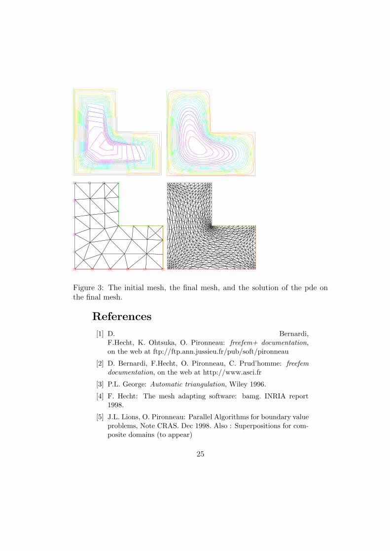
Figure 3: The initial mesh, the final mesh, and the solution of the pde onthe final mesh.

References

[1] D. Bernardi,F.Hecht, K. Ohtsuka, O. Pironneau: freefem+ documentation,on the web at ftp://ftp.ann.jussieu.fr/pub/soft/pironneau

[2] D. Bernardi, F.Hecht, O. Pironneau, C. Prud’homme: freefemdocumentation, on the web at http://www.asci.fr

[3] P.L. George: Automatic triangulation, Wiley 1996.

[4] F. Hecht: The mesh adapting software: bamg. INRIA report1998.

[5] J.L. Lions, O. Pironneau: Parallel Algorithms for boundary valueproblems, Note CRAS. Dec 1998. Also : Superpositions for com-posite domains (to appear)

25

[6] B. Lucquin, O. Pironneau: Scientific Computing for EngineersWiley 1998.

[7] F. Preparata, M. Shamos; Computational Geometry Springer se-ries in Computer sciences, 1984.

[8] R. Rannacher: On Chorin’s projection method for the incom-pressible Navier-Stokes equations, in ”Navier-Stokes Equations:Theory and Numerical Methods” (R. Rautmann, et al., eds.),Proc. Oberwolfach Conf., August 19-23, 1991, Springer, 1992

[9] J.L. Steger: The Chimera method of flow simulation, Workshopon applied CFD, Univ of Tennessee Space Institute, August 1991.

6 Appendix A: Details on the syntax

of freefeem+

6.1 Syntax of int

This keyword is used to computes integrals. It can be part of anarithmetic expression.

int([< mesh >]|[border[,border]n])(< expression >)

• If no borders are specified it is a surface (volume) integral. Elseit is a curve integral.

• Borders can be refered by their name or their reference number(defined by ”R2” and ”border”).

• If the mesh is not mentionned then the active mesh is used.

• The expression may involve arrays defined on another mesh.

• The quadrature uses the mid edge of the mesh/curve.

• The curve should be made of edges which are part of the meshused for the integral else the return value is zero, becausefreefem+ loops on the edges of the mesh, check if their labelis in the list and add the contribution of that edge to the result.

26

6.2 Syntax of ”solve”

solve([< mesh >, ] < array > [,array]n)[with < matrix > (< exp >)][< instruction >; ]n

pde(< array >)[< sign >] < operator > [∗|/ < exp >][< sign >< operator > [∗|/ < exp >]]n =< exp >;

on(< borderList >) < Dirichlet > | < Fourier >=< exp >;[on(< borderList >) < Dirichlet > | < Fourier >=< exp >; ]

In the above the | means ”or” and whe have

• ”mesh” is an existing mesh name

• ”array” is either a new variable (which then becomes of arraytype or an existing array variable. There can be more than 1,up to 5 in the present implementation (it is easy to put more).These will be refered as ”unknowns”.

• ”with” is useful if you intend to save computing time by reusingthe matrix factorized. It is imperative to check that no left handside has changed when you reuse a matrix, else the results willnot be correct.

• ”matrix” is a new variable or a variable previously declared asa matrix i.e. appearing at the same place in a solve statementearlier.

• the expression after ”matrix” will be treated as a boolean (is itzero or not?)

• if necessary regular instructions can be inserted within the solvestatement; it is usueful if they use the arrays declared after”solve”.

• for each unknown there must be a pde and its boundary condi-tions.

• each pde is restricted expression made of operators applied toany of the unknowns; pde(u) can involve dx(v)....

• ”borderList” is a list of names of borders separated by a commaand/or a list of integers which are the references to a set ofborders.

27

6.3 Syntax of ”on” within solve

< on > (< border > [, < border]n) < Dirichlet > | < Neumann >

< Dirichlet > ≡ < array >=< exp >

< Neumann > ≡ [< sign >] < op > [∗|/ < exp >][< sign >< op > [∗|/ < exp >]]n =< exp >

where ”op” is a boundary operator, i.e. either any unknown or dnu(X)and ”theUnknown” is X the variable inside pde(X).

6.4 Syntax of ”varsolve”

varsolve[(< mesh > [, < exp >])] < ident > (< ident >,< ident >

[, < ident >,< ident >]n)with < instruction >;

The following should be noted:

• If no mesh is specified, the default mesh is used. If the mesh isspecified it become the default mesh within the ”instruction”.

• The list of ”iden” between parenthesis is the variable list and thehat function list. Each variable is followed by its associated hatfunction.

• The ”instruction” should define the ”ident”. It is expected tobe a bilinear form in the variables. If it is not some kind ofunpredictable linearization with go on.

• The ”instruction” can be a block of instructions.

• To construct the matrix and linear system what freefem+ doesis to loop on each triangle, treat all variables as hat functions,assign to the hat functions a ”1” on one vertex, ”0” elsewhereand compute the value of the aa.

• The operator ”on” is a penalty operator, in this exemple it re-turns 107w(qj)(u(qj)− uΓ(qj)) at vertex qj .

6.5 Syntax of ”convect”

This operator performs one step of convection by the method ofCharacteristics-Galerkin. An equation like

∂tφ+ u∇φ = 0, φ(x, 0) = φ0(x)

28

is approximated by

1δt

(φn+1(x)− φn(Xn(x))) = 0

Roughly the term,φnoXn is approximated by φn(x− un(x)δt). Up toquadrature errors the scheme is unconditionnally stable. The syntaxis

< array >= convect(< exp1 >,< exp2 >,< exp3 >,< exp4 >)

• The ”array” is the result uoX;

• ”exp1” is the x-velocity,

• ”exp2” is the y-velocity of convection,

• ”exp3” is the time step,

• ”exp4 is the expression which is convected (u in the exempleabove)

Warning ”convect” is a non-local operator; in the instruction”phi=convec(u1,u2,dt,phi0)” every values of phi0 are used to computephi So ”phi=convec(u1,u2,dt,phi0)” won’t work won’t work.

6.6 Other keywords

To keyword ”plot” is used to display the level lines of a function orof an expression which returns an array or a function. It can displayseveral such pictures at once.

plot([< filename >, ][< mesh >, ] < expression >

[, [< mesh >, ] < expression >]n)

where the ”filename” is for a Postscript save of the displaid picture.

There are a number of formats to save meshes and arrays and freefemrespond to the suffixe of the file name given.

savemesh(” < filename > ”[, < meshname >])

The string is the file name and if no mesh is specified then the de-fault mesh is used. The suffix of the filename drives the format forcompatibility with other mesh generation programs.

save(” < filename > ”, < arrayname >)

29

Saves in ”filename” a function named by ”arrayname” on the activetriangulation.

To read meshes and array functions use

mesh < name >= readmesh(” < filename > ”);read(” < filename > ”, < arrayname >);

7 Appendix B: Line output for Exam-

ple 1

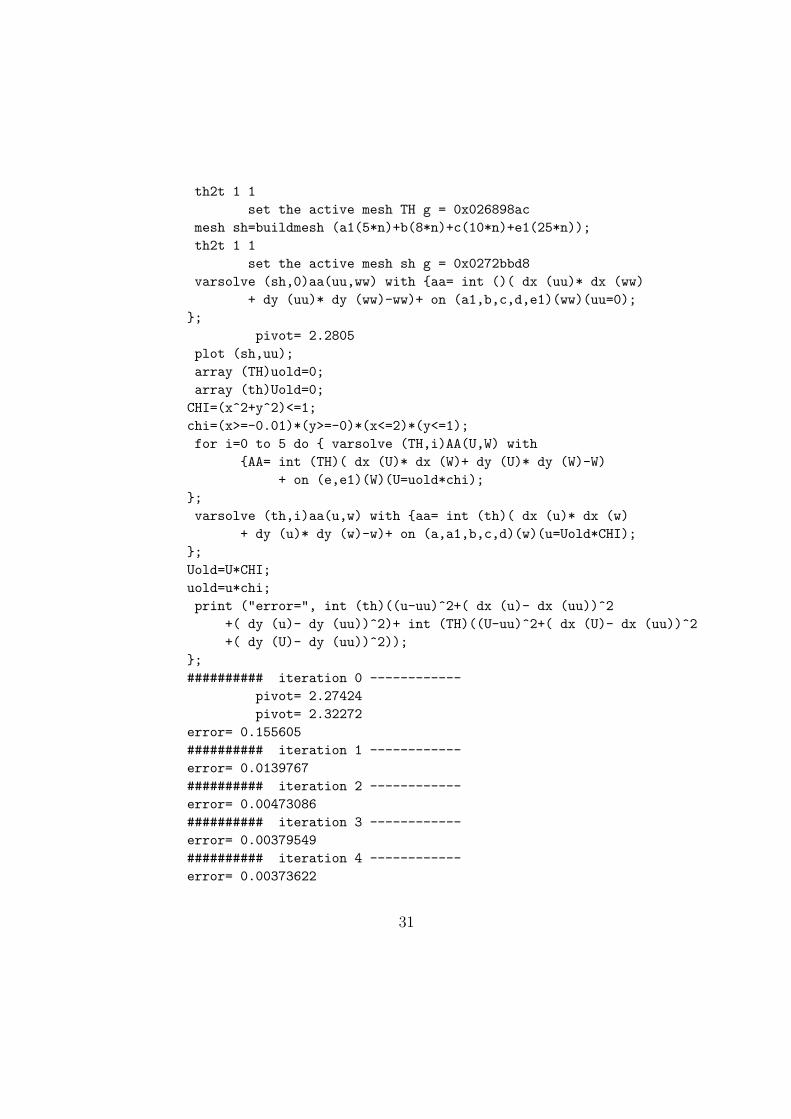
Freefem will display on the screen the source lines, some comments tohelp debugging and the requested text to be printed. For the Schwarzalgorithm 1 of above it gives:

Welcome to freefem+Start Program FreeFem+0.9.31

wait:=0;border a(t=0,1)x=t;y=0;border a1(t=1,2)x=t;y=0;border b(t=0,1)x=2;y=t;border c(t=2,0)x=t;y=1;border d(t=1,0)x=0;y=t;border e(t=0,pi/2)x=cos(t);y=sin(t);border e1(t=pi/2,2*pi)x=cos(t);y=sin(t);n:=4;mesh th=buildmesh ("th1",a(5*n)+a1(5*n)+b(5*n)+c(10*n)+d(5*n));

Save Postscript in file ’th1.ps’th2t 1 1

set the active mesh th g = 0x02692f1cmesh TH=buildmesh ("th2",e(5*n)+e1(25*n));

Save Postscript in file ’th2.ps’

30

th2t 1 1set the active mesh TH g = 0x026898ac

mesh sh=buildmesh (a1(5*n)+b(8*n)+c(10*n)+e1(25*n));th2t 1 1

set the active mesh sh g = 0x0272bbd8varsolve (sh,0)aa(uu,ww) with aa= int ()( dx (uu)* dx (ww)

+ dy (uu)* dy (ww)-ww)+ on (a1,b,c,d,e1)(ww)(uu=0);;

pivot= 2.2805plot (sh,uu);array (TH)uold=0;array (th)Uold=0;CHI=(x^2+y^2)<=1;chi=(x>=-0.01)*(y>=-0)*(x<=2)*(y<=1);for i=0 to 5 do varsolve (TH,i)AA(U,W) with

AA= int (TH)( dx (U)* dx (W)+ dy (U)* dy (W)-W)+ on (e,e1)(W)(U=uold*chi);

;varsolve (th,i)aa(u,w) with aa= int (th)( dx (u)* dx (w)

+ dy (u)* dy (w)-w)+ on (a,a1,b,c,d)(w)(u=Uold*CHI);;Uold=U*CHI;uold=u*chi;print ("error=", int (th)((u-uu)^2+( dx (u)- dx (uu))^2

+( dy (u)- dy (uu))^2)+ int (TH)((U-uu)^2+( dx (U)- dx (uu))^2+( dy (U)- dy (uu))^2));

;########## iteration 0 ------------

pivot= 2.27424pivot= 2.32272

error= 0.155605########## iteration 1 ------------error= 0.0139767########## iteration 2 ------------error= 0.00473086########## iteration 3 ------------error= 0.00379549########## iteration 4 ------------error= 0.00373622

31

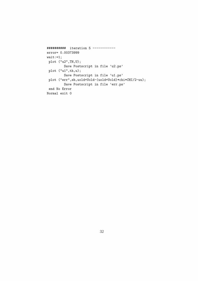
########## iteration 5 ------------error= 0.00373999wait:=1;plot ("u2",TH,U);

Save Postscript in file ’u2.ps’plot ("u1",th,u);

Save Postscript in file ’u1.ps’plot ("err",sh,uold+Uold-(uold+Uold)*chi*CHI/2-uu);

Save Postscript in file ’err.ps’end No ErrorNormal exit 0

32