multivariate data analysis of organochlorines and...

Multivariate Data Analysis of Organochlorinesand Brominated Flame Retardants in Baltic SeaSalmon (Salmo salar)

Gabriella Hernqvist

Degree project in biology, Bachelor of science, 2008Examensarbete i biologi 15 hp till kandidatexamen, 2008Biology Education Centre and Department of Physiology and Developmental Biology, UppsalaUniversitySupervisor: Katrin Lundstedt-Enkel

1

Abstract

This report contains information about contaminants in salmon caught in November in the

Baltic Sea, the year 2000. Concentrations of numerous types of organochlorines (OCs) and

brominated flame retardants (BFRs) in the salmons have been analyzed and studied using

multivariate data analysis. The report have four aims and the first aim is to determine the

concentrations, variations and patterns of pollutants. The second aim is to see if there are any

differences in contaminant pattern between the genders. The third aim is to look at

concentrations of pollutants eventual correlations to biological factors of the fish (e.g. length,

weight, condition factors and/or fat content). The last aim is to investigate if the

concentrations of OCs and BFRs co-varied with each other, if concentrations of OCs can be

used to calculate BFRs and vice versa.

DDE was the contaminant that reached the highest concentrations in both males

and females, with higher concentration then ∑PCB. The pollutants showed different patterns

in male and females, meaning that there is a difference in the contaminant patterns between

the genders. Several containments had significantly higher levels in females than in males.

Regarding the groupings of the contaminants when analyzing the contaminant concentration

data with principal component analysis several groups were formed, one with all BFRs and

OCs (excluding dioxins and furans, and “dioxin-like” polychlorinated bipenhyls (DL-PCBs)),

one group consisted of the DL-PCBs and the last was one more loosely formed group with the

dioxins and furans. The groupings show that the contaminants within the same group have the

same exposure routes, chemical reactivity, bioavailability, distribution, biotransformation,

and/or excretion thus co-varying to a high degree. The result shows that females have

significant higher lipid content than males. The concentration of BFRs and OCs co-varied

with each other a linear regression for instance between BDE47 and CB101, concentrations

showed a r2 of > 0.92 and a p-value of < 0.0001.

Sammanfattning

Den här rapporten innehåller information om lax som är infångad i november i Östersjön år

2000. Olika typer av organokloriner (OK) och bromerande flamskyddsmedel (BFM) har blivit

analyserade och studerade med hjälp av multivariat dataanalys. Rapporten är uppbyggd kring

fyra frågeställningar, varav den första frågan rör koncentrationer, variationer och mönster i

miljögifterna. Den andra är att undersöka om det finns det skillnader mellan könen. Den tredje

frågan handlar om det finns samband mellan miljögifter och laxarnas biologiska faktorer t ex

längd, vikt och fetthalt. Den sista frågeställningen undersöker om koncentrationerna av BFM

och OK samvarierar med varandra, om koncentrationen av BFM kan räknas ut med hjälp av

koncentrationen av OK och vice versa. DDE är det miljögift som når de högsta

koncentrationerna både i honor och i hanar med högre koncentration än ∑PCB. Miljögifterna

har olika koncentrationer i honor och hanar, vilket betyder att där är skillnad i

kontaminantmönstret mellan honor och hanar. Flera miljögifter hade högre nivåer i honor än

hanar. Vid principalkomponentanalys av alla föroreningars koncentrationer i laxarna skapades

grupperingar med olika miljögifter; en med BFM och OK (exkluderat dioxiner, furaner och

”dioxinliknande” polyklorerade bifenyler (DL-PCBer)), en grupp med DL-PCBer och en mer

löst formad grupp med dioxiner och furaner. Denna gruppering indikerar att vissa ämnen

inom samma grupp har samma exponeringsvägar, kemisk reaktivitet, biotillgänglighet,

biotransformation och/eller exkretion, vilket leder till en hög grad av kovarians. Honorna har

signifikant högre fetthalt än hanarna. Koncentrationerna av BFM och OK kovarierade med en

varandra; linjär regression till exempel mellan BDE47 och CB101 visar ett r2värde > 0.92 och

ett p-värde < 0.0001.

2

Contents

INTRODUCTION ................................................................................................................................................. 4

BALTIC SEA ........................................................................................................................................................ 4 SALMON (SALMO SALAR) ...................................................................................................................................... 4 CONTAMINANTS .................................................................................................................................................. 5

Organochlorines ............................................................................................................................................ 5 Brominated Flame Retardants ....................................................................................................................... 6 Dioxins and furans ........................................................................................................................................ 7

TEF & TEQ ........................................................................................................................................................ 8

AIMS ...................................................................................................................................................................... 9

MATERIAL AND METHODS .......................................................................................................................... 10

SALMON ............................................................................................................................................................ 10 CONTAMINANT ANALYSIS ................................................................................................................................. 10 STATISTICS ........................................................................................................................................................ 11

Basic Statistics ............................................................................................................................................. 11 Multivariate statistics .................................................................................................................................. 11

RESULTS ............................................................................................................................................................ 13

CONCENTRATIONS OF OCS AND BFRS .............................................................................................................. 13 DIFFERENCES DUE TO GENDER .......................................................................................................................... 20 RELATIONSHIP BETWEEN BIOLOGICAL VARIABLES AND THE CONTAMINANTS ................................................... 21 THE RELATIONSHIPS BETWEEN OCS AND BFRS ................................................................................................ 23

DISCUSSION ...................................................................................................................................................... 25

ACKNOWLEDGMENTS .................................................................................................................................. 27

REFERENCES .................................................................................................................................................... 27

3

Abbreviations BFR Brominated flame retardants

BFM Bromerade flamskyddmedel (in Swedish)

DDD Dichlorodiphenyldichloroethane

DDE Dichloroethylene

DDT Dichlorodiphenyltrichloro-ethane

FR Flame retardant

HBCD Hexabromocyclododecane

MVDA Multivariate data analysis

OC Organochlorines

OK Oragnokloriner (in Swedish)

PBB Polybrominated biphenyls

PBDE Polybrominated diphenyl ethers

PCA Principal component analysis

PCB Polychlorinated bipenhyls

PLS Partial least squares regression projection to latent structures

POP Persitant organic pollutants

TBBPA Tetrabromobisphenol-A

TCDD Tetrachlorodibenzodioxin

TEF Toxic equivalency factors

TEQ Toxic equivalency quotient

VIP Variable influences on projection

4

Introduction The Baltic Sea has during the last century been contaminated with various pollutants through

the activities of man; via eutrophication [1] and industry [2]. In the Baltic Sea the pollutants

get incorporated in the food chain and affects living organisms [3]. Some persistent

contaminants biomagnify to top predators [4] and can reach high levels in piscivorous fish

like the salmon. Salmon serve as an important food source and the Swedish Food

Administration recommends that one eat fish three times a week [5, 6], because of its

nutritional value e.g. that fish contains long chains of essential omega-3 fatty acids [6].

Knowing current pollutant levels is of great importance, for example when giving food

recommendations to the public or specific risk groups like pregnant women. Pollution may

lead to severe damages in an already threatened environment like the Baltic Sea [7] and basic

data regarding levels and trends as well as effects caused by pollutants are needed. Especially

before one can start to regulate the use of certain chemicals.

This report is about salmon caught in the Baltic Sea and is focusing on four

different aims. The first aim is to look at the contaminants analyzed in the salmon muscle; to

determine concentrations, to discern variations and patterns among different pollutants. The

second aim is to see if there are any differences between the genders. The third aim is to look

at concentrations of pollutants and their correlation to biological factors of the fish e.g. length,

weight, and/or lipid content. The fourth aim is to investigate if the concentrations of

organochlorines (OCs) and brominated flame retardants (BFRs) co-varied with each other, if

concentrations of OCs can be used to calculate BFRs and vice versa.

Baltic Sea

The Baltic Sea is the largest sea with brackish water in the world. The sea consist of several

basins with various depth and the only communication with the North Sea is through the

narrow and shallow Öresund and the Belt Sea [8]. The Baltic Sea drainage area includes 14

densely populated and industrial countries, where about 90 million people live. The Sea

contains both hard- and soft-bottoms, with bladder wrack Fucus vesiculosus and the blue

mussel Mytilus edulis as the dominant species of hard-bottoms and the Baltic macoma

Macoma balthica as a dominant species of the soft-bottom. The salinity is declining from the

south towards the north, leading to a rapid decrease in the biomass and number of species

towards the north [3]. The severe ecosystem in the Baltic Sea leads to high physiological

stress, causing increased sensitivity to pollutants [9].

Salmon (Salmo salar)

The salmon was named Salmo salar by Linné in the year 1758. The salmon in the Baltic Sea

is hatched in several different rivers, lives there for a few years and then transforms from

spawn to smolt and emerge to the Baltic Sea or in the lake Vänern with its surrounding

waters. Vänern is a large fresh water lake in Sweden. In the rivers young salmons is

characterized by 8-10 blue-green dots along the sides with red dots in between. As an adult

the salmon lives either in the sea or in Vänern. The adult salmon has a grey-silverish color,

with black x-shaped or circle dots above the collateral line. Before spawning the males get a

colorful costume and the lower jaw transforms into a hook, while the females get a less

colorful costume. Maximum weight and length for salmon is 35-40 kg and 130-150 cm

respectively. At the end of 1990 there were 40 rivers in Sweden with an annual natural

reproduction of wild salmon. Compensation rearing of salmon (spawn and smolt) has been

performed in numerous waters to improve the populations. The human influence have the last

decades been a severe treat to the wild salmon eg. development of hydropower, pollution and

5

changes in the biotope. Since the 1800-century wild populations has disappeared from smaller

waters and in the 2000-century also from larger. An ongoing exploitation of rivers may lead

to the disappearance of even more populations. Recreation of spawning- and growth areas

have lead to an improvement in the reproduction situation and a weak increase in salmon

spawning has been seen. More improvements for the salmon are planned and the development

of the salmon population growth will be monitored. The salmon is classified as endangered by

the Swedish Species Information Center, for more information see www.artdata.slu.se [10].

Today, all Swedish salmon contain pollutants to such a degree that salmon meat exceeds the

limiting value set by the EU, which is a TEQ of 8 pg/g (ww) for all dioxins and DL-PCBs.

The Swedish Food Administration now recommend the females and children (both boys and

girls) only consume wild caught salmon from the Baltic Sea or lake Vänern 2-3 times/ year.

Contaminants

All the contaminants in this report are chlorinated or brominated organic substances so called

organochlorines (OCs) and brominated flame retardants (BFRs). Among the OCs some

compounds are classified as persistent organic pollutants (POPs). To deal with these kind of

compounds the Stockholm Convention of Persistant Organic Pollutations adopted a text on

the 22 May 2001, which later was entered into force the 17 May 2004 [11]. All compounds

listed as POPs share four properties; they are highly toxic, accumulate in fat tissue, they have

the ability to travel long distance in air and water and they are persistent. Visit www.pops.int

for further information. In this report the following compounds, which also are in the list of

“The first 12 POPs”, are included; DDT, dioxins, furans, HCB and PCBs [12].

Organochlorines

From the mid- 1940s OCs agents were used widely in a numbers of various aspects e.g.

agriculture, forestry and to control insect pests. Some OCs make up an efficient group of

insecticides because of the chemical structure; chemical stability, lipid solubility, slow rate of

biotransformation and degradation. These properties lead to persistence in the nature, and an

accumulation of concentration and possible biomagnification within various food chains [13].

DDT, DDE, DDD and PCB

DDT (dichlorodiphenyltrichloro-ethane) was first synthesized by Zeidler in 1874 and it was

rediscovered when searching for an insecticide against clothes moths and carpet beetles [14].

The use of DDT has many advantages; it is extremly toxic to insects but less toxic to other

animals, it has a low production cost, it is persistent thus continuing its insecticidal properties

for a very long time. In history as well as today in many developing countries DDT has been

used for control of malaria and other insect-borne diseases. DDE (dichloroethylene) is a

metabolite of DDT, resulting from the loss of one chlor and one hydrogen atom (see Figure

1). It doesn’t serve as an insecticide like DDT because of its low toxicity to insects. DDE is

the most common chlorinated hydrocarbon in the sea and in marine organisms, as a result of

metabolism of DDT. DDD (dichlorodiphenyldichloroerthane) is another metabolite of DDT.

DDD has been used as an insecticide because it has lower toxicity to fish than DDT. Due to

its chemical and physical characteristics it can be excreted by organisms and rarely

accumulates, like DDE [8].

Dr D.A. Ratcliff showed in 1967 that DDT causes thinning of eggshells,

resulting in reproductive failure. This caused the declining in the white-tailed eagle

(Haliaeetus albicilla) population in Sweden, and after the prohibition of DDT and PCB it took

over ten years before the eagle population started to recover [15]. p,p’DDT and p,p’DDE

display oestrogenic activity and areas contaminated with these substances have declining

6

animal populations. For instance, the alligator populations in Florida show sexual

abnormalities and have eggs that fail to hatch. The alligators had low levels of DDE (0.01

ppm) not enough for causing toxic effects but enough to disrupt the endocrine system [3].

Cl

Cl

Cl

Cl Cl Cl Cl

Cl Cl

Cl Cl

Cl Cl

p,p’DDT p,p’DDE p,p’DDD

Figure 1. Chemical structure of p,p’DDT, p,p’DDE and p,p’DDD.

PCBs (polychlorinated bipenhyls) have been used since the 1930s as flame

retardants in electric equipment, in paints and in plastics as it is resistant to chemical attacks.

The number of chlorine atoms at one PCB-molecule varies from one to ten and these can be

differently positioned on the two phenyl rings (Figure 4) giving 209 possible so called

congeners. A rising concern about environmental damage from chlorinated hydrocarbon

pesticides affected the use of PCBs as well. A reduction of manufacturing of PCB started in

1970 and by the mid-1980s most members of the European Union had stopped the production.

But even though the manufacture has been restricted today, the concentrations are still high in

the environment [8].

PCB has affected several species in the Baltic Sea. Mammals all over the world

like seals, sea lions and otters have had declining populations. It is suggested that the high

levels of PCB in seals is responsible for a failure of reproduction. There was an accident in

Japan were rice oil became contaminated with PCB which caused darkening of the skin in

humans, enlargement of hair follicles and eruptions of the skin resembling acne. Similar

symptoms have also been observed in workers in Japan, and their symptoms disappeared

when the use of PCBs ceased. Exposure to PCB and p,p’DDE from consumption of fat fish

from the Baltic Sea has shown to effect human sperm quality [16].

(Cl)n(Cl)

n

Figure 2. Chemical structure of PCB.

Brominated Flame Retardants

BFRs are an umbrella term for organic compounds which contains bromine and prevent the

spreading of fire and increase the time for a fire to ignite. They are used for example in

electronic equipment, textiles, construction materials and furniture. The use has increased

dramatically over the last decades [17]. BFRs are an umbrella term for organic compounds

which contains bromine. Some groups of BFRs are; TBBPA (Tetrabromobisphenol-A),

HBCD (Hexabromocyclododecane), PBDEs (Polybrominated diphenyl ethers) and PBB

(Polybrominated biphenyls) (see Figure 3).

7

Concerns, has risen because of the BFRs persistence, bioaccumulation and

toxicity, in human and animals. Due to the industrial use, BFR have been released in to the

surrounding environment, mainly via equipment that has been treated with BFR. BFR can

now be found everywhere in water, sediment, animals and human tissue. BFR is lipophilic

and accumulates in the bodies’ fat tissue [18]. PBDE have a biomagnification potential in the

food chain in the Baltic Sea ecosystem [11]. Major exposure routes to human are dietary

intake, dust inhalation and occupational exposure. Uptake via food are of great importance,

especially consumption of meat, fish and dairy products. Fish is of great concern, due to high

levels of PBDE [19]. There is only a limit of studies made on toxicity to humans. One study

showed higher-than-normal prevalence of primary hypothyroidism and a reduction on

conducting velocities in sensory and motor neurons. Hypothyroidism is a disease caused by

insufficient production of thyroid hormones [18]. Viberg et al. ,2004, have showed that PBDE

can cause a behavioural neurotoxic effect and affect cholinergic receptors in mice [20].

Brn Br

n

TBBPA PBDE PBB HBCD

Figure 3. Chemical structure of TBBPA, PBDE, PBB and HBCD.

Dioxins and furans

Dioxins (PCDD) and furans (PCDF) consist of two groups; chlorinated dioxins (75

congeners) containing one to eight chlorine atoms, were the congener TCDD (2,3,7,8-

tetrachlorodibenzodioxin) is of greatest interest due to its high toxicity. The second group,

chlorinated dibenzofurans has a similar structure but contains 135 congener (Figure 4).

Dioxins are a side product in the wood processing industry and when producing herbicides.

They are extremely toxic, physically and chemically stable and soluble in organic solvent, fat

and oil. These characters makes dioxins and furans an important group to eliminate, and some

of the sources has been reduced or eliminated [8].

Evidence of dioxins being damaging to humans, is rather inconclusive. One

accident, when there was an explosion in a pesticide factory, and the surroundings became

showered with dioxin, lead to chloracne, minor but reversible nerve damage, and some

impaired liver functions. Studies have been made to reveal a link between dioxins and soft

tissue sarcomas, but this cancer type has been rare and so far the link hasn’t been confirmed

[3].

O

OCl

n Cln

O

Cln

Cln

Dioxin (PCDD) Furan (PCDF)

Figure 4. Chemical structure of dioxins and furans.

O

Brn Br

n

Br

Br

Br

Br

Br

Br

H3C CH

3

Br Br

Br BrHO OH

8

TEF & TEQ

Toxic equivalency factors (TEF) is a measurement of toxicity for dioxin-like compounds. In

this report several compounds are included that have dioxinlike modes of action, both dioxins,

furans and also “dioxin-like” PCBs (DL-PCBs). For a compound to be included in the TEF

concept these criteria must been reached [21]:

show a structure relationship to the PCDDs and PCDFs

bind to the aryl hydrocarbon receptor (AhR)

elicit Ah-receptor-mediated biochemical and toxic response

be persistent and accumulate in the food chain

TEF-values are used by the World Health Organisation (WHO) as a method to evaluate

toxicities of mixtures consisting of dioxins and furans as well as DL-PCBs.As 2,3,7,8-TCDD

is one of the most studied and also one of the most toxic congener, it therefore has a TEF-

value set to one. Then the other dioxins/furans and DL-PCBs are given TEF-values that show

their respective toxicity in relation to TCDD. TEF-values is a useful tool for determine risks

from mixtures of dioxin compounds. Toxic equivalency quotient (TEQ) is a measurement

were the concentration of each compound is taken into account multiplied with its TEF-value.

TEQ-value is calculated according to this formula [22]:

𝑇𝐸𝑄 = 𝑐𝑖 ∗ 𝑇𝐸𝐹

𝑛

TEQ=value for toxicity of a mixture of compounds n=numbers of compounds

ci=concentration of each compound

TEF=a value for toxicity for each compound taken from WHO [21]

9

Aims The report contains several aims:

The first aim is to look at the contaminants; to determine concentrations, to discern

variations and patterns among different pollutants.

The second aim is to determine if there are any differences between the genders.

The third aim is to look at concentrations of pollutants and their correlation to

biological factors of the fish e.g. length, weight and/or lipid content.

The fourth aim is to investigate if the concentrations of OCs and BFRs co-varied with

each other, if concentrations of OCs can be used to calculate BFRs and vice versa.

10

Material and Methods

Salmon

In this report a total of 17 salmons (Salmon salar) are included that were caught in the Baltic

Sea, in November the year 2000, near Gotland will be used. The salmons’ biological variables

(see Table 1) were; smolt age, sex, body weight (BW), body length (excluding tail fin (BL)

and including tail fin (TBL), separately), condition factor (Cond. F.), liver weight (LW), liver

somatic index (LSI), brain weight (BrW) and lipid content (F%). Condition factors were

calculated as BW/TBL3. Liver somatic index is calculated as LW/BW*100. The origin of the

fish, either wild or reared was noted.

Table 1. Biological data (mean ± st.dev, min - max) for salmon (Salmo salar) (n=17) caught in the Baltic Sea,

the year 2000. BW= body weight, BL=Body length excluding tail fin, TBL= Total body length including tail fin,

Cond. F.= Condition factor (BW/TBL3), LW=Liver Weight, LSI=Liver Somatic Index (LW/BW*100),

BrW=Brain Weight and F%=Lipid content.

Females Males P-value

n=10 n=7 Female vs. male1

Smolt age2 year

Mean ± St Dev

Min – Max

2.20 ± 0.42

2.00 – 3.00

2.00 ± 0.0

2.00 – 2.00 ns

BW g Mean ± St Dev

Min – Max

4159 ± 461.3

3328 – 4960

3728±593.5

2945 - 4561 ns

BL cm Mean ± St Dev

Min – Max

62.25 ± 2.05 60.93 ± 4.99 ns

58.00 – 64.00 54.00 – 68.00

TBL cm Mean ± St Dev

Min – Max

71.35 ± 2.36 69.36 ± 4.42 ns

66.00 – 74.00 62.00 – 76.00

Cond. F. g/cm3

Mean ± St Dev

Min - Max

1.143 ± 0.03 1.11 ± 0.08 ns

0.99 – 1.28 1.00 – 1.24

LW g Mean ± St Dev

Min - Max

50.40 ± 7.89 52.71 ± 15.33 ns

39.00 – 63.00 31.00 – 73.00

LSI % Mean ± St Dev

Min - Max

1.22 ± 0.16 1.41 ± 0.31 ns

0.96 – 1.43 1.05 – 1.89

BrW2

g Mean ± St Dev

Min - Max

0.80 ± 0.055 0.69 ± 0.13 ns

0.73 – 0.88 0.46 – 0.83

F% % Mean ± St Dev

Min - Max

12.61 ± 3.95 7.93 ± 3.74 0.027

5.95 – 18.40 4.76 – 14.37 1t-test

2n=15 for BrW and Smolt age

Contaminant analysis

The following OCs and BFRs were analysed (dioxins, furans and DL-PCBs are presented in

table 2); trans-nona chlor (t-n Chlor), 2,2-bis(4-chlorophenyl)-1,1,1-tri-chloroethane (p,p’-

DDT) and its’metabolites p,p’-DDE and p,p’-DDD, polychlorinated biphenyls (PCBs) with

the congeners’; 2,4,4´ tri-CB (CB28), 2,2´,5,5´ tetra-CB (CB52), 2,2´,4,5,5´penta-CB

(CB101), 2,3,3’,4,4’-penta-CB (CB105), 2,3’,4,4’,5-penta-CB (CB118), 2,2´,3,4,4´,5´hexa-

CB (CB138), 2,2´, 4,4´,5,5´hexa-CB (CB153), 2,3,3’,4,4’,5-hexa-CB (CB156),

2,2´,3,4,4´,5,5´hepta-CB (CB-180), hexachlorocyclohexane (isomers α-, β-, and γ-HCH), and

hexachlorobenzene (HCB). The BFRs were; hexabromocyclododecane (HBCD) and the

polybrominated diphenyl ethers (PBDEs): 2,2´,4,4´tetra-BDE (BDE47), 2,2´,4,4´,5 penta-

BDE (BDE99), 2,2´,4,4´,6 penta-BDE (BDE100), 2,2´,4,4´,5,5´ hexa-BDE (BDE153), and

2,2´,4,4´,5,6´ hexa- BDE (BDE154). ∑HCH was calculated as the sum of α-HCH, β-HCH and

γ-HCH concentrations, ∑DDT was calculated as the sum of p,p’DDT, p,p’DDE and p,p’DDD

11

concentrations, ∑PCB as the sum of ICES 7 marker PCBs’: CB28, CB52, CB101, CB118,

CB138, CB153 and CB180 concentrations and ∑PBDE as the sum of BDE cogeners BDE47,

BDE99, BDE100, BDE153 and BDE154. The contaminants are presented both in lipid weight

(lw) and wet weight (ww) and if that not specified concentrations are always given as wet

weight. Analysed PCDD/DF and DL-PCBs, their abbreviations and their corresponding TEF

values are presented separately in Table 2.

The chemical analyses was carried out by Swedish Museum of Natural History

(for the organochlorines, excluding dioxins and furans), at Applied Enviromental Science

(ITM) at Stockholm University (for the brominated flame retardants) and at Enviromental

Chemistry at Umeå University (for the dioxins, furans and DL-PCBs). Table 2. Analyzed dioxins, furans and DL-PCBs, their abbreviation and TEF-values for contaminants included in

this report.

Analyzed substances Abbreviations TEF1

Chlorinated dibenzo-p-dioxins

2,3,7,8-TCDD TCDD 1

1,2,3,7,8-PeCDD PeCDD 1

1,2,3,4,7,8-HxCDD HxCDD1 0.1

1,2,3,6,7,8-HxCDD HxCDD2 0.1

1,2,3,7,8,9-HxCDD HxCDD3 0.1

1,2,3,4,6,7,8-HpCDD HpCDD 0.01

OCDD OCDD 0.0003

Chlorinated dibenzofurans

2,3,7,8-TCDF TCDF 0.1

1,2,3,7,8-PeCDF PeCDF1 0.03

2,3,4,7,8-PeCDF PeCDF2 0.3

1,2,3,4,7,8-HxCDF HxCDF1 0.1

1,2,3,6,7,8-HxCDF HxCDF2 0.1

2,3,4,6,7,8- HxCDF HxCDF3 0.1

1,2,3,7,8,9- HxCDF HxCDF4 0.1

1,2,3,4,6,7,8-HpCDF HpCDF1 0.01

1,2,3,4,7,8,9-HpCDF HpCDF2 0.01

OCDF OCDF 0.0003

Non-ortho-PCBs

3,3´,4,4´-tetraCB CB77 0.0001

3,4,4´,5-tetraCB CB81 0.0001

3,3´,4,4´,5-pentaCB CB126 0.00003

3,3’,4,4’,5,5’-hexaCB CB169 0.03 1Values based on the article by Van den Berg et al. 2006 [21].

Statistics

Basic Statistics

For statistic regarding the biological variables and concentrations of OCs and BFRs the

software GraphPad Prism 5.01 [23] was used. This included calculations of the geometric

mean (GM), 95% confidence interval (lower and upper), arithmetic mean values (Mean),

standard deviation (St. Dev.), minimum (Min), maximum (Max), correlation analysis

(Pearson), un-paired two-tailed t-test, Kolmogorov-Smirnov normality test, D’Agostino and

Pearson omnibus normality test and Shapiro-Wilk normality test. The significance level was

set to 0.05 for all the tests.

Multivariate statistics

Multivariate data analysis (MVDA) is a useful tool when handling data which has three or

more variables, i.e. columns for each individual animal with measured or analysed values.

12

Two types of MVDA have been used; principal component analysis (PCA) and partial least-

squares projection to latent structures (PLS). MVDA were performed using the software

SIMCA-P +11 [24] and for all MVDA a significance level of 0.05 was used.

PCA was used to illustrate the data and to discover groupings in the data among

the contaminants as well as grouping according to gender. Values of the explained variation

(R2) and predicted variation (Q

2) were calculated. R

2 values >0.7 and Q

2 values >0.4 denote

an acceptable model when analyzing biological data [25].

PLS was used to determine whether there were a significant relationship

between biological factors and contaminants. PLS was also used to investigate if the

concentrations of OCs and BFRs co-varied with each other. PLS is an extension of multiple

linear regressions similar to PCA but it is used to model the relationship between two

matrixes, Y and X, that can both be multidimensional.

13

Results

Concentrations of OCs and BFRs

Concentrations as geometric mean (GM) ± 95% confidence interval (-Cl and+Cl) in salmon

are presentented in Table 3 and Table 4. The contaminants with the highest concentration in

both females and males is p,p’DDE with a concentration almost as high as ∑PCB. When

looking at the sum of different contaminants they will be arranged as followed:

∑DDT>∑PCB>∑HCH>∑PBDE both when considering lipid weight, wet weight and females

and males separately.

Table 3. Concentrations (ng/g) as geometric mean (GM) with lower and upper 95% confidence interval (-Cl) and

(+Cl) of organochlorines and brominated flame retardants in salmon (Salmo salar) (females n=10 and males

n=7) muscle from the Baltic Sea, near Gotland, the year 2000. For abbreviations see Materials and Methods.

Females

n=10

ng/g

Males

n=7

ng/g

GM -Cl +Cl GM -Cl +Cl

αHCH Lipid weight 10.69 10.34 11.05 10.55 9.863 11.28

Wet weight 1.284 0.954 1.729 0.8154 0.558 1.192

βHCH Lipid weight 16.28 15.61 16.97 15.51 14.20 16.94

Wet weight 1.940 1.473 2.555 1.215 0.823 1.793

γHCH Lipid weight 8.082 7.685 8.499 7.849 7.491 8.224

Wet weight 0.975 0.769 1.237 0.605 0.411 0.891

∑HCH1 Lipid weight 35.05 33.64 36.52 33.91 31.55 36.44

Wet weight 4.199 3.200 5.521 2.635 1.792 3.876

HCB Lipid weight 24.73 21.75 28.11 24.27 21.68 27.16

Wet weight 3.019 2.178 4.185 1.844 1.330 2.556

t-n Chlor Lipid weight 19.65 17.19 22.47 22.50 17.87 28.31

Wet weight 2.407 1.792 3.233 1.670 1.192 2.340

CB28 Lipid weight 3.120 2.639 3.689 2.479 1.906 3.226

Wet weight 0.378 0.286 0.498 0.195 0.140 0.273

CB522

Lipid weight 15.29 13.26 17.64 14.61 12.22 17.47

Wet weight 1.983 1.667 2.357 1.107 0.806 1.521

CB773

Lipid weight 1.041 0.848 1.278 0.892 0.565 1.408

Wet weight 0.119 0.761 0.186 0.069 0.025 0.189

CB813 Lipid weigh 0.016 0.012 0.023 0.015 0.010 0.022

Wet weight 0.002 0.001 0.003 0.012 0.001 0.003

CB101 Lipid weight 58.54 51.09 67.08 58.42 47.56 71.77

Wet weight 7.119 5.338 9.495 4.449 3.301 5.996

CB105 Lipid weight 22.10 19.56 24.96 21.66 17.06 27.51

Wet weight 2.678 2.177 3.296 1.660 1.160 2.374

CB118 Lipid weight 60.87 53.95 68.68 57.65 46.07 72.15

Wet weight 7.377 5.858 9.290 4.437 3.212 6.129

CB1263

Lipid weight 0.451 0.360 0.564 0.420 0.303 0.581

Wet weight 0.051 0.032 0.081 0.033 0.013 0.079

CB138 Lipid weight 113.6 100.3 128.6 122.5 98.63 152.3

Wet weight 13.74 10.89 17.33 9.298 6.681 12.94

CB153 Lipid weight 143.8 127.2 162.6 158.3 127.9 195.8

Wet weight 17.46 13.58 22.44 11.93 8.751 16.27

CB156 Lipid weight 0.008 0.007 0.009 0.008 0.007 0.011

Wet weight 0.001 0.001 0.001 0.001 nd 0.001

CB1693

Lipid weight 0.075 0.060 0.095 0.087 0.058 0.130

Wet weight 0.009 0.005 0.014 0.007 0.003 0.013

14

CB180 Lipid weight 41.38 36.28 47.19 50.21 37.98 66.38

Wet weight 5.006 3.934 6.371 3.753 2.687 5.242

∑PCB4

Lipid weight 436.6 384.7 495.5 464.2 372.3 579.1

Wet weight 70.52 41.55 67.78 35.17 25.58 48.37

p,p’DDE Lipid weight 364.4 308.3 430.6 368.9 305.3 445.6

Wet weight 45.05 32.75 61.96 27.52 20.60 36.77

p,p’DDD Lipid weight 154.9 128.7 186.5 126.1 85.03 186.9

Wet weight 19.21 14.23 25.94 9.634 6.527 14.22

p,p’DDT Lipid weight 77.19 62.03 96.06 73.53 55.00 98.29

Wet weight 9.568 6.620 13.83 5.512 3.933 7.726

∑DDT5

Lipid weight 596.5 499.0 713.2 568.53 445.3 730.8

Wet weight 73.83 53.60 101.7 42.666 31.11 58.72

PBDE47 Lipid weight 20.26 16.90 24.28 19.92 17.09 23.23

Wet weight 2.506 1.801 3.487 1.491 1.094 2.033


Wet weight 0.466 0.325 0.666 0.2577 0.186 0.357


Wet weight 0.411 0.306 0.554 0.2765 0.205 0.373


Wet weight 0.076 0.056 0.104 0.04761 0.036 0.063


Wet weight 0.079 0.059 0.107 0.05608 0.044 0.071

∑PBDE6

Lipid weight 28.63 23.67 34.64 28.451 23.81 34.08

Wet weight 3.539 2.546 4.919 2.1289 1.565 2.898

HBCD Lipid weight 15.20 12.60 18.33 13.86 10.55 18.20

Wet weight 1.872 1.343 2.609 1.052 0.800 1.384 1∑HCH= sum of αHCH, βHCH and γHCH concentrations.

2n=9 for females

3n=6 for females and n=5 for males

4∑PCB= sum of ICES marker PCBs: CB28, CB52, CB101, CB118, CB138, CB153 and CB180

5∑DDT= sum of p,p’DDT, p,p’DDE and p,p’DDD

6∑PBDE= sum of BDE congeners: BDE47, BDE99, BDE100, BDE153 and BDE154

Figure 5-6 illustrate the concentrations of chlorinated contaminants, female and male

respectively. In Figure 5 all the analyzed OCs are shown though the DL-PCB cogeners are

shown in Figure 6 seperatly. All the contaminants are shown on both lipid (A) and wet weight

(B) basis in the different graphs. When considering PCBs on wet weight basis there is a

significant different in concentration in some of the contaminants between females and males

A B

Figure 5. Concentration (ng/g) of clorinated contaminats in A lipid weight and B wet weight in salmon (S. salar)

(females n= 10 and males n=7) muscle from the Baltic Sea, the year 2000.

aHCH

bHCH

gHCH

HCB

t-n C

hlor

CB28

CB52

CB10

1

CB10

5

CB11

8

CB13

8

CB15

3

CB15

6

CB18

0DDE

DDD

DDT

0

20

40

60

80

Female

Male

Co

ncen

trati

on

(n

g/g

ww

)

aHCH

bHCH

gHCH

HCB

t-n C

hlor

CB28

CB52

CB10

1

CB10

5

CB11

8

CB13

8

CB15

3

CB15

6

CB18

0DDE

DDD

DDT

0

100

200

300

400

500

Female

Male

Co

ncen

trati

on

(n

g/g

lw

)

15

A B

PCB 8

1

PCB 7

7

PCB 1

26

PCB 1

69

0

500

1000

1500Female

Male

Co

ncen

trati

on

(p

g/g

lw

)

Figure 6. Concentration (pg/g) of clorinated contaminats in A, lipid weight and B, wet weight in salmon (S.

salar) (n=6 for females and n=5 for males) muscle from the Baltic Sea, the year 2000.

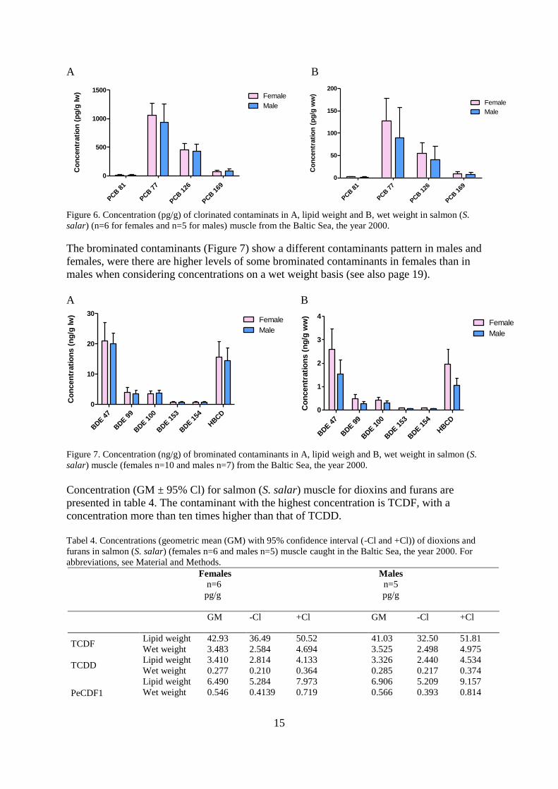
The brominated contaminants (Figure 7) show a different contaminants pattern in males and

females, were there are higher levels of some brominated contaminants in females than in

males when considering concentrations on a wet weight basis (see also page 19).

A B

Figure 7. Concentration (ng/g) of brominated contaminants in A, lipid weigh and B, wet weight in salmon (S.

salar) muscle (females n=10 and males n=7) from the Baltic Sea, the year 2000.

Concentration (GM ± 95% Cl) for salmon (S. salar) muscle for dioxins and furans are

presented in table 4. The contaminant with the highest concentration is TCDF, with a

concentration more than ten times higher than that of TCDD.

Tabel 4. Concentrations (geometric mean (GM) with 95% confidence interval (-Cl and +Cl)) of dioxions and

furans in salmon (S. salar) (females n=6 and males n=5) muscle caught in the Baltic Sea, the year 2000. For

abbreviations, see Material and Methods.

Females

n=6

pg/g

Males

n=5

pg/g

GM -Cl +Cl GM -Cl +Cl

TCDF Lipid weight 42.93 36.49 50.52 41.03 32.50 51.81

Wet weight 3.483 2.584 4.694 3.525 2.498 4.975

TCDD Lipid weight 3.410 2.814 4.133 3.326 2.440 4.534

Wet weight 0.277 0.210 0.364 0.285 0.217 0.374

PeCDF1

Lipid weight 6.490 5.284 7.973 6.906 5.209 9.157

Wet weight 0.546 0.4139 0.719 0.566 0.393 0.814

BDE 4

7

BDE 9

9

BDE 1

00

BDE 1

53

BDE 1

54

HBCD

0

1

2

3

4Female

Male

Co

ncen

trati

on

s (

ng

/g w

w)

BDE 4

7

BDE 9

9

BDE 1

00

BDE 1

53

BDE 1

54

HBCD

0

10

20

30Female

Male

Co

ncen

trati

on

s (

ng

/g lw

)

PCB 8

1

PCB 7

7

PCB 1

26

PCB 1

69

0

50

100

150

200

Female

Male

Co

ncen

trati

on

(p

g/g

ww

)

16

PeCDF2 Lipid weight 34.81 29.02 41.75 41.95 25.83 68.14

Wet weight 2.903 2.183 3.859 3.388 2.419 4.745

PeCDD Lipid weight 5.937 4.944 7.130 6.762 4.869 9.389

Wet weight 0.486 0.374 0.632 0.560 0.425 0.737

HxCDF1 Lipid weight 0.896 0.663 1.209 0.941 0.705 1.256

Wet weight 0.075 0.060 0.095 0.077 0.054 0.109


Wet weight 0.102 0.077 0.134 0.101 0.063 0.163


Wet weight 0.077 0.055 0.106 0.081 0.055 0.120


Wet weight 0.013 0.008 0.022 0.012 0.011 0.013

HxCDD1 Lipid weight 0.236 0.177 0.314 0.244 0.194 0.308

Wet weight 0.020 0.016 0.025 0.020 0.017 0.023


Wet weight 0.183 0.143 0.236 0.217 0.159 0.297


Wet weight 0.017 0.010 0.026 0.028 0.020 0.038

HpCDF1 Lipid weight 0.164 0.121 0.223 0.166 0.122 0.226

Wet weight 0.013 0.011 0.016 0.014 0.013 0.015

HpCDF2 Lipid weight 0.189 0.139 0.258 0.198 0.145 0.272

Wet weight 0.015 0.013 0.018 0.017 0.015 0.018

HpCDD Lipid weight 0.285 0.209 0.388 0.338 0.253 0.452

Wet weight 0.023 0.020 0.028 0.028 0.022 0.035

OCDF Lipid weight 0.264 0.198 0.354 0.279 0.211 0.370

Wet weight 0.021 0.018 0.026 0.024 0.022 0.026

OCDD Lipid weight 1.907 1.313 2.767 2.045 1.366 3.059

Wet weight 0.146 0.108 0.198 0.181 0.1588 0.205

Furans and dioxins are illustrated in Figure 8, female and male respectively. All the

contaminants are shown both on lipid and wet weight basis.

A B

Figure 8. Concentration (pg/g) of furans and dioxions in A lipid weight and B wet weight in salmon muscle (S.

salar) (females n=10 and males n=7) from the Baltic Sea, the year 2000.

The PCA analysis (R2X = 0.849 and Q

2 = 0.58, three components) reveals the formation of

two groups, males and females (Figure 9A). Even though there is some overlap between the

two genders, this indicates a difference in contaminant patterns between females and males.

Figure 9B show a formation of four different groups of contaminants. One homogenous group

TCDF

TCDD

PeC

DF1

PeC

DF2

PeC

DD

HxC

DF1

HxC

DF2

HxC

DF3

HxC

DF4

HxC

DD1

HxC

DD2

HxC

DD3

HpC

DF1

HpC

DF2

HpC

DD

OCDF

OCDD

0

20

40

60

80

Female

Male

Co

ncen

trati

on

(n

g/g

lw

)

TCDF

TCDD

PeC

DF1

PeC

DF2

PeC

DD

HxC

DF1

HxC

DF2

HxC

DF3

HxC

DF4

HxC

DD1

HxC

DD2

HxC

DD3

HpC

DF1

HpC

DF2

HpC

DD

OCDF

OCDD

0

2

4

6

Female

Male

Co

ncen

trati

on

(n

g/g

ww

)

17

of brominated flame retardants and “ordinary” organochlorines (excluding furans and dioxins,

and DL-PCBs). The rest of the contaminants are divided into three groups one with the DL-

PCBs, and two other groups with the lower chlorinated dioxins and furans and one with the

higher chlorinated ones. Alternative these may create a more “loosly” formed group with all

dioxins and furans.

B

Figure 9. Principal component analysis (PCA) including the concentrations of contaminants (wet weight) in

salmon (S. salar) muscle from Gotland, Baltic Sea, (females n=10 males n=7). PCA model (R2X = 0.849 and Q

2

= 0.58, three components), (a) scatter plot with the two classes, males (M) (dots) and females (F) (sqaures) (b)

loading plot. For abbreviations, see Materials and Methods.

The PLS analysis (R2X = 0.591, R

2Y=0.382 and Q

2 = 0.219, one component) with female and

male as Y and all the contaminants (wet weight) as X, show that there is a positive correlation

between higher concentration of several of the contaminants and being a female (Figure 10).

-6

-4

-2

0

2

4

6

-14 -12 -10 -8 -6 -4 -2 0 2 4 6 8 10 12 14

t [c

om

ponent 2]

t [component 1]

Scatter plot

R2X[1] = 0.600888 R2X[2] = 0.149216

F

F

F

F

F

F

F

FF

F

M

M

M

M

M

M

M

-0,3

-0,2

-0,1

-0,0

-0,1 0,0 0,1 0,2

p [com

ponent 2]

p [component 1]

Loading plot

R2X[1] = 0.600888 R2X[2] = 0.149216

aHCHwbHCHwgHCHwHCBw

t-n ChlorwCB 28w

CB 52wCB 101w

CB 105wCB 118w

CB 138wCB 153wCB 156w

CB 180w

DDEw

DDDwDDTw

BDE 47wBDE 99w

BDE 100w

BDE 153w

BDE 154w

HBCDDw

TCDF w

TCDD wPeCDF1 w

PeCDF2 w

PeCDD wHxCDF1 w

HxCDF2 wHxCDF3 w

HxCDF4 w

HxCDD1 w

HxCDD2 w

HxCDD3 wHpCDF1 w

HpCDF2 w

HpCDD w

OCDF w

OCDD w PCB 81 w

PCB 77 wPCB 126 w

PCB 169 w

-0,10

-0,08

-0,06

-0,04

-0,02

0,00

0,02

0,04

0,185 0,190 0,195 0,200 0,205 0,210

p [com

ponent 2]

p [component 1]

Loading plot

R2X[1] = 0.600888 R2X[2] = 0.149216

aHCHwbHCHw

gHCHw

HCBw

t-n Chlorw

CB 28w

CB 52wCB 101w

CB 105wCB 118w

CB 138w

CB 153w

CB 156w

CB 180w

DDEw

DDDw

DDTw

BDE 47w

BDE 99w

BDE 100w

BDE 153w

BDE 154w

HBCDDw

18

Figure 10. Coefficient plot with 95% Cl for the respective variables for PLS model (R2X = 0.591, R

2Y=0.382

and Q2 = 0.219, one component) between gender (here females) and concentrations of organochlorines and

brominated flame retardants in salmon (S. salar) muscle (n=17) from the Baltic Sea. For abbreviations see

Materials and Method.

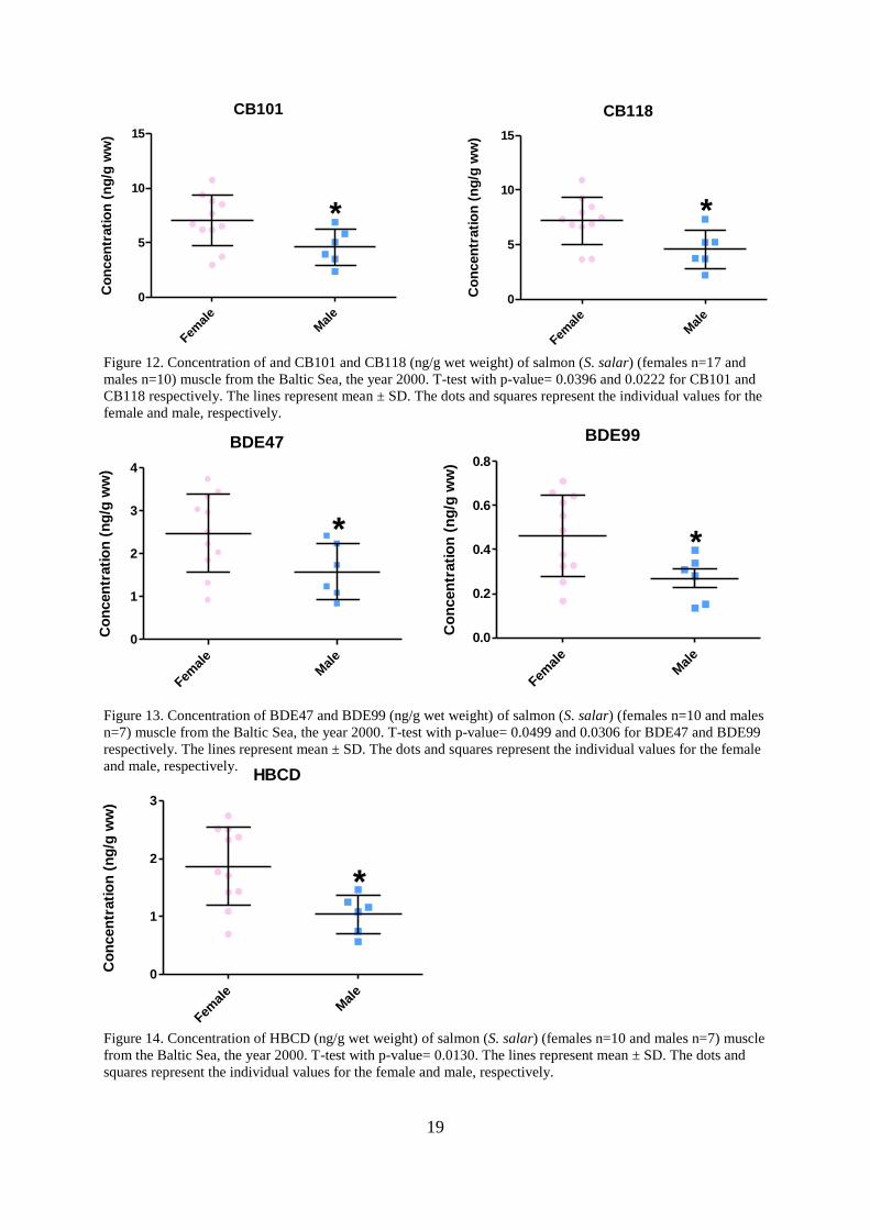
There are significant differences between some of the contaminants between female and male,

see Figure 11-14. Females has a significant (one-way t-test) higher values of p,p’DDD (p-

value 0.0158), p,p’DDT (p-value 0.0369) (Figure 11), CB101 (p-value=0.0396), CB118 (p-

value=0.0222) (Figure 12), BDE47 (p-value= 0.0499), BDE99 (p-value=0.0306) (Figure 13)

and HBCD (p-value=0.0130) (Figure 14). There was no significant difference in TEQ-values

between males and females. The following contaminants are included in the TEQ calculation;

all dioxions, furans and DL-PCBs (those contaminants in Table 2).

Figure 11. Concentration of DDD and DDT (ng/g wet weight) of salmon (S. salar) (females n=10 and males

n=7) muscle from the Baltic Sea, the year 2000. T-test with p-value= 0.0158 and 0.0396 for DDD and DDT and

respectively. The lines represent mean ± SD. The dots and squares represent the individual values for the female

and male, respectively.

-0,05

-0,04

-0,03

-0,02

-0,01

0,00

0,01

0,02

0,03

0,04

0,05

HxC

DD

3 w

HpC

DD

wH

xCD

D2

wH

pCD

F2

wO

CD

F w

PeC

DF

2 w

PeC

DD

wH

xCD

F2

wH

xCD

F3

wH

pCD

F1

wO

CD

D w

HxC

DD

1 w

PeC

DF

1 w

HxC

DF

1 w

TC

DD

wT

CD

F w

HxC

DF

4 w

PC

B 1

69 w

PC

B 1

26 w

PC

B 7

7 w

PC

B 8

1 w

CB

180

wt-

n C

hlor

wC

B 5

2wB

DE

100

wC

B 1

53w

BD

E 1

54w

aHC

Hw

CB

138

wD

DE

wgH

CH

wD

DT

wH

CB

wbH

CH

wB

DE

47w

BD

E 1

53w

CB

105

wB

DE

99w

CB

101

wC

B 1

56w

HB

CD

Dw

DD

Dw

CB

118

wC

B 2

8w

Coe

ffici

ents

; com

p. 1

(fe

mal

e)

Femal

e

Mal

e

0

10

20

30

40

DDD

Co

ncen

trati

on

(n

g/g

ww

)

*

Femal

e

Mal

e

0

5

10

15

20

DDT

Co

ncen

trati

on

(n

g/g

ww

)

*

19

Figure 12. Concentration of and CB101 and CB118 (ng/g wet weight) of salmon (S. salar) (females n=17 and

males n=10) muscle from the Baltic Sea, the year 2000. T-test with p-value= 0.0396 and 0.0222 for CB101 and

CB118 respectively. The lines represent mean ± SD. The dots and squares represent the individual values for the

female and male, respectively.

Figure 13. Concentration of BDE47 and BDE99 (ng/g wet weight) of salmon (S. salar) (females n=10 and males

n=7) muscle from the Baltic Sea, the year 2000. T-test with p-value= 0.0499 and 0.0306 for BDE47 and BDE99

respectively. The lines represent mean ± SD. The dots and squares represent the individual values for the female

and male, respectively.

Figure 14. Concentration of HBCD (ng/g wet weight) of salmon (S. salar) (females n=10 and males n=7) muscle

from the Baltic Sea, the year 2000. T-test with p-value= 0.0130. The lines represent mean ± SD. The dots and

squares represent the individual values for the female and male, respectively.

BDE99

Femal

e

Mal

e

0.0

0.2

0.4

0.6

0.8C

on

cen

trati

on

(n

g/g

ww

)

*

CB118

Femal

e

Mal

e

0

5

10

15

Co

ncen

trati

on

(n

g/g

ww

)

*

HBCD

Femal

eM

ale

0

1

2

3

Co

ncen

trati

on

(n

g/g

ww

)

*

CB101

Femal

e

Mal

e

0

5

10

15

Co

ncen

trati

on

(n

g/g

ww

)

*

BDE47

Femal

eM

ale

0

1

2

3

4

*

Co

ncen

trati

on

(n

g/g

ww

)

20

Differences due to gender

The biological variables (mean ± St. Dev, min - max) for salmon are presented in Table 1.

Univariate statistics testing female vs. male for each biological variable separately showed no

significant differences between the sexes except for lipid content (Table 1 and Figure 15). The

lipid content is significant higher (p-value= 0.02) in females than in males.

Femal

eM

ale

0

5

10

15

20

*

Lip

id c

on

ten

t %

Figure 15. Graph with the lipid content as % in salmon (S. salar) muscle (females n=10 and males n=7) from the

Baltic Sea, near Gotland, the year 2000. T-test with P-value= 0.023. The lines represent mean ± SD. The dots

and squares represent the individual values for the female and male, respectively.

21

Relationship between biological variables and the contaminants

The only biological variable that co-varied with the contaminant concentrations was the lipid

content. The PLS (R2X = 0.691, R

2Y = 0.939, Q

2= 0.791) model in Figure 16 show that the

lipid content has a positive relationship with a number of PCBs e.g. CB138, t-n chlor and

CB180 as well as with αHCH, βHCH and γHCH. Figure 17 show a linear regression between

lipid content and t-n Chlor, CB138 and CB180, all with p-values < 0.0001. The regression

coeifficients are: 0.8155, 0.8284, 0.7055 for t-n Chlor, CB138 and CB180 respectively.

A

B

Figure 16. Partial least squares regression to latent structures (PLS) model (R2X = 0.691, R

2Y = 0.939, Q

2=

0.791, two components) between fat content (F%) and concentrations of contaminants (ng/g ww) in salmon

(Salmo salar) muscle from the Baltic Sea, the year 2000 (n=17). (A) Loading plot (B) Coefficent plot with lipid

content (F%) as Y and all contaminants on wet weight basis as X . For abbreviations see Material and Method.

0,00

0,02

0,04

0,06

0,08

0,10

0,12

0,14

0,16

0,20 0,21 0,22

w*c

[com

ponent 2]

w*c [component 1]

Loading plot

R2X[1] = 0.570162 R2X[2] = 0.1209

XY

HCBwt-n Chlorw

CB 52w

CB 101w

CB 105w

CB 118w

CB 138wCB 153w

CB 156w

CB 180w

DDEw

BDE 47wBDE 100w

F%

-0,10

-0,05

-0,00

0,05

0,10

aH

CH

wbH

CH

wgH

CH

wH

CB

wC

B 1

38w

CB

153w

t-n C

hlo

rwC

B 1

05w

CB

180w

CB

156w

CB

118w

CB

52w

CB

101w

BD

E 1

00w

HpC

DF

1 w

BD

E 4

7w

DD

Ew

OC

DF

wC

B 2

8w

HpC

DF

2 w

HB

CD

Dw

TC

DF

wD

DT

wD

DD

wH

xC

DD

1 w

TC

DD

wsum

CD

F w

sum

D+

F w

BD

E 9

9w

OC

DD

wH

xC

DD

3 w

PeC

DF

1 w

sum

CD

D w

BD

E 1

54w

BD

E 1

53w

HxC

DF

3 w

PeC

DF

2 w

PeC

DD

wH

xC

DD

2 w

HxC

DF

2 w

HxC

DF

4 w

HpC

DD

wH

xC

DF

1 w

PC

B 7

7 w

PC

B 8

1 w

PC

B 1

26 w

PC

B 1

69 w

Coeffic

ients

; com

p. 1 (

F%

)

-0,3

-0,2

-0,1

-0,0

0,1

0,2

0,3

-0,1 0,0 0,1 0,2

w*c

[com

ponent 2]

w*c [component 1]

Loading plot

R2X[1] = 0.570162 R2X[2] = 0.1209

XY

aHCHwbHCHwgHCHw

HCBwt-n Chlorw

CB 28w

CB 52wCB 101w

CB 105w

CB 118w

CB 138wCB 153wCB 156w

CB 180w

DDEw

DDDwDDTw

BDE 47w

BDE 99w

BDE 100w

BDE 153wBDE 154w

HBCDDw

TCDF w

TCDD wPeCDF1 w

PeCDF2 wPeCDD w

HxCDF1 wHxCDF2 w

HxCDF3 w

HxCDF4 w

HxCDD1 wHxCDD2 w

HxCDD3 w

HpCDF1 wHpCDF2 w

HpCDD w

OCDF w

OCDD w

sumCDD wsumCDF wsum D+F w

PCB 81 wPCB 77 w

PCB 126 w

PCB 169 w

F%

22

Figure 17. The relationship between lipid content (%) and t-n chlor, CB138 and CB180 in salmon (S.salar)

muscle (n=17) caught in the Baltic Sea, near Gotland, the year 2000, p-value < 0.0001, r2=0.82, 0.83, 0.71 for t-n

Chlor, CB138 and CB180 respectively.

Figure 16 also shows that there is no correlation between several PCDD/DF and the lipid

content e.g. HpCDF2 and OCDF. To further illustrate this figure 18 show a linear regression

between lipid content and HpCDF2 and OCDF, p-value= 0.561 and 0.681 for HpCDF2 and

OCDF respectively. R2= 0.04 and 0.02 for HpCDF2 and OCDF respectively.

0 5 10 15 200.012

0.014

0.016

0.018

0.020r2=0.039p<0.5617

Lipid content (%)

Hp

CD

F2 c

on

cen

trati

on

(p

g/g

ww

)

0 5 10 15 200.015

0.020

0.025

0.030 r2= 0.020p= 0.681

Lipid content (%)

OC

DF

(p

g/g

ww

)

Figure 18. The relationship between lipid content (%) and HpCDF2 and OCDF in salmon (S. salar) muscle

(n=17), caught in the Baltic Sea, near Gotland, the year 2000, p-value= 0.56 and 0.68, r2=0.04, and 0.02 for

HpCDF2 and OCDF respectively.

0 5 10 15 200

5

10

15

20

r2=0.8284p<0.0001

Lipid content (%)

CB

138 c

on

cen

trati

on

(n

g/g

ww

)

0 5 10 15 200

2

4

6

8

r2=0.7055p<0.0001

Lipid content (%)

CB

180 c

on

cen

trati

on

(n

g/g

ww

)

0 5 10 15 200

1

2

3

4

r2=0.8155p<0.0001

Lipid content (%)

t-n

Ch

lor

co

ncen

trati

on

(n

g/g

ww

)

23

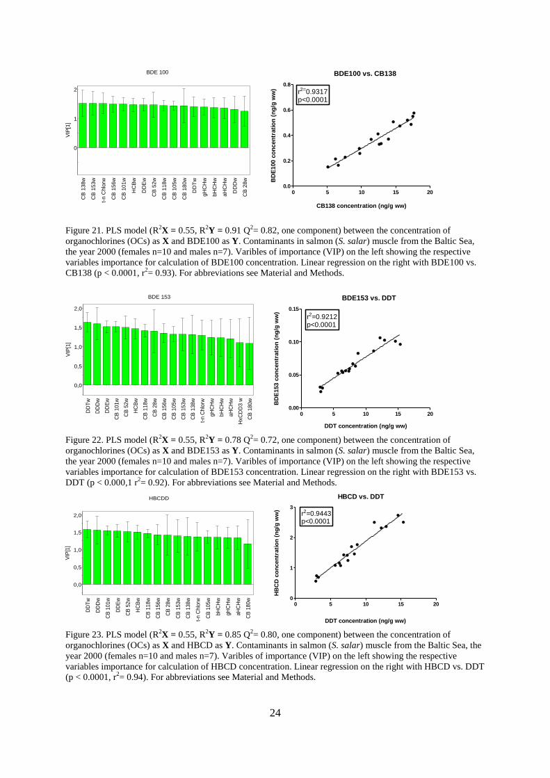
The relationships between OCs and BFRs

Figures 19-23 show result from the PLS model (R2X = 0.549, R

2Y = 0.924, Q

2= 0.882, one

component) that shows the relationship between several brominated contaminants and

chlorinated contaminants. The variable influences on projection (VIP) plots on the left show

the variables of importance for calculation of BDE47, BDE99, BDE100, BDE153 and HBCD,

respectively. A linear regression, showing the relationship between one brominated

contaminant and one chlorinated, can be seen in Figures 18-22 on the right. The linear

regressions all have a p-value < 0.0001 and r2

> 0.92.

0 5 10 150

1

2

3

4

5r2=0.9371p<0.0001

BDE47 vs. CB101

CB101 concentration (ng/g ww)

BD

E47 c

on

cen

trati

on

(n

g/g

ww

)

Figure 19. PLS model (R

2X = 0.549, R

2Y = 0.924, Q

2=0.882, one component) between the concentration of

organochlorines (OCs) as X and BDE47 as Y. Contaminants in salmon (S. salar) muscle from the Baltic Sea, the

year 2000 (females n=10 and males n=7). Varibles of importance (VIP) on the left showing the respective

variables importance for calculation of BDE47 concentration. Linear regression on the right with PBDE vs. CB

101 (p < 0.0001, r2= 0.9371). For abbreviations see Material and Methods.

0 5 10 15 200.0

0.2

0.4

0.6

0.8

r2=0.9489p<0.0001

BDE99 vs. DDT

DDT concentration (ng/g ww)

BD

E99 c

on

cen

trati

on

(n

g/g

ww

)


2X =0.548, R

2Y = 0.803 Q

2= 0.741, one component) between the concentration of

organochlorines (OCs) as X and BDE99 as Y. Contaminants in salmon (S. salar) muscle from the Baltic Sea, the


variables importance for calculation of BDE 99 concentration. Linear regression on the right with BDE99 vs.

DDT (p < 0.000,1 r2= 0.9489). For abbreviations see Material and Methods.

-0,5

0,0

0,5

1,0

1,5

2,0

CB

101w

DD

Ew

HC

Bw

CB

52w

DD

Tw

CB

156w

CB

118w

CB

153w

CB

138w

DD

Dw

t-n C

hlo

rw

CB

105w

gH

CH

w

bH

CH

w

aH

CH

w

CB

28w

CB

180w

VIP

[1]

BDE 47

-0,5

0,0

0,5

1,0

1,5

2,0

DD

Tw

DD

Dw

DD

Ew

CB

101w

CB

52w

HC

Bw

CB

118w

CB

28w

CB

156w

CB

153w

CB

138w

CB

105w

t-n C

hlo

rw

gH

CH

w

bH

CH

w

aH

CH

w

VIP

[1]

BDE 99

24

0 5 10 15 200.0

0.2

0.4

0.6

0.8

r2=0.9317p<0.0001

BDE100 vs. CB138

CB138 concentration (ng/g ww)

BD

E100 c

on

cen

trati

on

(n

g/g

ww

)

Figure 21. PLS model (R2X = 0.55, R

2Y = 0.91 Q


organochlorines (OCs) as X and BDE100 as Y. Contaminants in salmon (S. salar) muscle from the Baltic Sea,

the year 2000 (females n=10 and males n=7). Varibles of importance (VIP) on the left showing the respective

variables importance for calculation of BDE100 concentration. Linear regression on the right with BDE100 vs.

CB138 (p < 0.0001, r2= 0.93). For abbreviations see Material and Methods.

0 5 10 15 200.00

0.05

0.10

0.15

r2=0.9212p<0.0001

BDE153 vs. DDT


BD

E153 c

on

cen

trati

on

(n

g/g

ww

)


2X = 0.55, R

2Y = 0.78 Q


organochlorines (OCs) as X and BDE153 as Y. Contaminants in salmon (S. salar) muscle from the Baltic Sea,

the year 2000 (females n=10 and males n=7). Varibles of importance (VIP) on the left showing the respective

variables importance for calculation of BDE153 concentration. Linear regression on the right with BDE153 vs.

DDT (p < 0.000,1 r2= 0.92). For abbreviations see Material and Methods.

0 5 10 15 200

1

2

3

r2=0.9443p<0.0001

HBCD vs. DDT


HB

CD

co

ncen

trati

on

(n

g/g

ww

)


2X = 0.55, R

2Y = 0.85 Q


organochlorines (OCs) as X and HBCD as Y. Contaminants in salmon (S. salar) muscle from the Baltic Sea, the


variables importance for calculation of HBCD concentration. Linear regression on the right with HBCD vs. DDT

(p < 0.0001, r2= 0.94). For abbreviations see Material and Methods.

0

1

2

CB

138w

CB

153w

t-n C

hlo

rw

CB

156w

CB

101w

HC

Bw

DD

Ew

CB

52w

CB

118w

CB

105w

CB

180w

DD

Tw

gH

CH

w

bH

CH

w

aH

CH

w

DD

Dw

CB

28w

VIP

[1]

BDE 100

0,0

0,5

1,0

1,5

2,0

DD

Tw

DD

Dw

DD

Ew

CB

101w

CB

52w

HC

Bw

CB

118w

CB

28w

CB

156w

CB

105w

CB

153w

CB

138w

t-n C

hlo

rw

gH

CH

w

bH

CH

w

aH

CH

w

HxC

DD

3 w

CB

180w

VIP

[1]

BDE 153

0,0

0,5

1,0

1,5

2,0

DD

Tw

DD

Dw

CB

101w

DD

Ew

CB

52w

HC

Bw

CB

118w

CB

156w

CB

28w

CB

153w

CB

138w

t-n C

hlo

rw

CB

105w

bH

CH

w

gH

CH

w

aH

CH

w

CB

180w

VIP

[1]

HBCDD

25

Discussion The first aim was to look at the contaminants; to determine concentrations, to discern

variations and patterns among different pollutants. The sum of concentrations arranged from

the highest to the lowest looks as followed; ∑DDT>∑PCB>∑HCH>∑PBDE. The

contaminants with the highest sum are the compounds and their metabolites which have been

used longest by man. DDT and PCB has been used almost 80 years [8, 13] while PBDE is a

rather new FR and wasn´t established as a new major chemical FR until the year 1978 [19].

The use of OCs and increasing use of BFRs will probably lead to a change in the sum of the

contaminants as well as their relative order. Szlinder-Richert et al. [26] showed in their article

regarding contaminants in e.g. salmon from the Polish Baltic Sea a level of ∑HCH (~ 20 ng/g

lw) that is lower than the level presented in this report (~ 34-35 ng/g lw). The article also

showed a downward trend from ~23 to ~15 between the years 2003 and 2006. The salmons in

this report are from 2000, so there might be a general downward trend in concentrations of

HCH, which correspond well with the result from Szlinder-Richert et al. The sum of DDT in

Szlinder-Richert et al. article varied between 1700 (ng/g lw) to 777 (ng/g lw) between the

year 2003 and 2006. The concentrations of ∑DDT show a large fluctuate between the years;

no clear trends can be seen. These concentrations compared to the 585 (ng/g lw) in the present

article is a little bit higher which is interesting since DDT has been prohibited 40 years [15]

meaning that DDT levels should decline. The high DDT concentration might be an indication

that DDT is still in use in Poland or in other eastern-european countries. This show that DDT

is still a treat to the environment, due to its slow degradation, and that DDT has to be

monitored even though it has been prohibited. All the values in Szlinder-Richert et al. article

is presented as arithmetic mean compared to the concentrations in this article which is

presented as geometric mean. Arithmetic mean has always a higher values than geometric

mean when calculated on the same data since “outliers” with high concentrations affect the

arithmetric mean stronger than when calculating the geometric mean. In geometric mean

calculations outliers doesn’t have the same dramatic influence of the result. Figure 9B

indicate that contaminants with similar exposure routes, chemical reactivity, bioavailability,

distribution, biotransformation, and/or excretion form different groups with strong co-

variation between the contaminants within each group. There are one homogenous group of

brominated flame retardants and “ordinary” organochlorines (excluding furans and dioxins,

and DL-PCBs). The rest of the contaminants are divided into three groups one with the DL-

PCBs, and two other groups with lower and higher chlorinated dioxins and furans,

respectively. This strong co-variation is the reason why the OC concentration could be used to

calculate the individual’s BFR concentrations with such high accuracy (r2>0.92) (see aim 4).

The second aim was to see if there are any differences between the genders.

There is a significantly difference between the genders when considering lipid content (Figure

15). The significantly higher lipid content in females may cause a higher risk for

bioaccumulation of POPs, since one of the properties for POPs is an accumulation in fat

tissue. In this report this is confirmed by the results showing several contaminants which have

significant higher levels in female salmon when considering the contaminant concentrations

on a wet weight basis. Wet weight is also of greatest interest when dealing with salmon as a

food source. These results indicate that further investigations that separates between females

and males are of great interest. This is also of interest for salmon farming since it has been

shown earlier that reared salmon has greater lipid content than wild salmon [27]. Would the

human exposure to contaminants from salmon farming be lower with a different sex ratio,

favoring males or leaner fish? In the report several contaminants has been presented which

has significant higher values in females than in males. But even though there was a difference

26

between the genders, regarding many contaminants, there were no significant differences

between the genders when considering the TEQ-values on wet weight basis. Also, males seem

to have proportionally higher concentrations of dioxins and furans than females (Figure 10).

The scatter plot reveals information regarding the grouping between individuals. This gives a

good feed-back system, indicating that one individual classified as a female, actually could be

a male (since the contaminant pattern remind more of a male than a female). Unfortunately

this can’t be controlled in this study. The gonads should perhaps have been investigated using

a microscope instead of a stereomicroscope that was used here with much lower resolution.

The third aim is to look at concentrations of pollutants and their correlation to

biological factors of the fish e.g. length, weight and/or lipid content. There was only one

biological factor that correlated with the contaminants, and that was the lipid content (see

Figure 16). There are some important factors to take into concern when trying to understand

why the lipid content is co-varying with many contaminants; the administration, distribution,

metabolism and excretion, also known as the ADME of the contaminants. The administration

between the animals is probably almost the same, though a fatter individual may have had

more food. The distribution of contaminants vary a lot, contaminants can be accumulated in

the fat, in the organs or in the blood. The contaminants can travel around in the body or have a

specific target organ or tissue where it stays. The metabolism of contaminants can vary both

between different compounds but also between individuals. A healthy and young individual

probably have a faster metabolism, than an old sick individual. When considering pollutants it

is not unusual to find individuals which have a higher level of contaminants than what is the

mean even extremely high concentrations can be found in few individuals (~10-15 times the

mean) [28]. Excretion of compounds is dependent on its chemical properties, a water soluble

compounds is rather easily excreted by the kidneys via the urine. When a fat soluble

compounds can be incorporated in the body´s fat tissue as well as being excreted via the liver

and the bile and for fish, the compound can be excreted via gills. Some of the substances

which are not correlated with lipid content are classified as POPs e.g.the dioxins, furans and

DL-PCBs.

The fourth aim is to investigate if the concentrations of OCs and BFRs co-varied

with each other, if concentrations of OCs can be used to calculate BFRs and vice versa. The

result showed a strong correlation between brominated containments and chlorinated

containments in the Baltic Sea salmon.This relationship between BFRs and OCs has been

shown before in adult guillemot (Uria aalge), see Supporting Information to Lundstedt-Enkel

et al., 2005 [29]. This suggests that these contaminants have similar ADME routes in the

animals. The high r2 and low p-values mean that the co-variation between these pollutions is

strong. If some of the OCs can be calculated from the levels of BFRs, it could be of great

economic interest. Saving some of the cost for sample analysis and using the model to

calculate levels instead. If more reports included the relationships between BFRs and OCs

reliable models for calculations of OCs could be done rather easily. This OCs-BFRs model

will have to be validated at close intervals as the general levels of OCs is declining while the

general level of BFRs especially for HBCD are increasing.

27

Acknowledgments I would like to thank the Swedish Museum of Natural History, Applied Enviromental Science

(ITM) at Stockholm University, Umeå University and the Swedish Food Administration for

providing me data from the chemical analyses which this report is based on. The most

important part in the making of this report has been my tutor, Katrin Lundstedt-Enkel at the

department of Enviromental Toxicology Uppsala Univeristy, she has supported my,

encouraged me and explained every little bit of the complex world of multivariate data

analysis over and over again. Thank you for opening my eyes to a new fascinating world.

Finally, a thank you to the division of Environmental Toxicology, your friendly atmosphere is

a good help when Simca is like Greek.

References 1. Elmgren, R., Man´s Imapct on the Ecosystem of the Baltic Sea: Energy Flows Today

and at the Turn of the century. Ambio, 1989. 18(6): p. 326-332.

2. Lehtinen, K.-J., M. Notini, J. Mattson, and L. Landner, Disappearance of Bladder-

Wrack (Fucus vesiculosus L.) in the Baltic Sea: Relation to Pulp-Mill Chlorate.

Ambio, 1988. 17: p. 387-393.

3. Kautsky, L. and N. Kautsky, The Baltic Sea, Including Bothnian Sea and Bothnian

Bay, in Seas at the Millennium: An Environmental Evaluation 2000.

4. Dietz, R., F. Riget, M. Cleemann, A. Aarkrog, P. Johansen, and J.C. Hansen,

Comparison of contaminants from different trophic levels and ecosystems. The

Science of The Total Environment, 2000. 245(1-3): p. 221-231.

5. Wulf, B., L. Niels, P. Agnes, A. Antti, F. Mikael, T. Inga, A. Jan, A. Sigmund, M.

Helle, and P. Jan, Nordic Nutrition Recommendations 2004 - integrating nutrition and

physical activity. Scandinavian Journal of Nutrition, 2004. 48: p. 178-187.

6. National Food Administration, [Accessed June 2008], www.slv.se

7. WWF, Breathless Coastal Seas WWF Briefing Paper: Dead Ocean Zones - a global

Problem of the 21st century. 2008

8. Clark, R.B., Marine Pollution. Fitfh ed. 2001, New York: Oxford University Press

Inc.

9. Tedengren, M., M. Arnér, and N. Kautsky, Ecophysiology and stress response of

marine and brackish water Gammarus species (Crustacea, Amphipopda) to changes in

salinity and exposure to cadmium and diesel-oil. Marine Ecology Progress Series,

1988. 47: p. 107-116.

10. Jansson, H., P. Nyberg, and A. Johlander, Faktablad: Salmo Salar - gullspångslax.

2006 In Swedish.

11. Lundstedt-Enkel, K., P.M. Lek, and J. Örberg, QSBMR - Quantitative Structure

Biomagnification Relationships: Physiochemical and Structural Descriptors Important

for the Biomagnification of Organochlorines and Brominated Flame Retardants

Journal of Chemometrics, 2006. 20(8-10): p. 392 -401.

12. United Nations Environment Programme., Ridding the World of POPs: A Guide to the

Stockholm Convention on Persistant Organic Pollutants. 2005.

13. Ecobichon, J.D., Toxic Effects of Pesticides, in Casarett and Doull's Toxicology: The

Basic Science of Poisons, C.D. Klaassen, Editor. 2001, McGraw-Hill. p. 763-772.

14. Ecobichon, J.D., Toxic Effects of Pestcides, in Casarett and Doull's Toxicology: The

Basic Science of Poisons, C.D. Klaassen, Editor. 1996, McGraw-Hill.

15. Helander, B., Faktablad: Haliaeetus albicilla – havsörn. 2006 In Swedish

16. Rignell-Hydbom, A., L. Rylander, A. Giwercman, B.A.G. Jönsson, C. Lindh, P.

Eleuteri, M. Rescia, G. Leter, E. Cordelli, M. Spano, and L. Hagmar, Exposure to

http://www.slv.se/

28

PCBs and p,p′-DDE and Human Sperm Chromatin Integrity. Environmental Health

Perspectives, 2005. 113: p. 175-179.

17. Birnbaum, L.S. and D.F. Staskal, Brominated Flame Retardants: Cause for Concern?

Environ Health Perspectives, 2004. 112: p. 9-17.

18. Darnerud, P.O., E. Gunnar S., J. Torkell, L. Poul B., and V. Matti, Polybrominated

diphenyl ethers: Occurrence, Dietary Exposure, and Toxicology. Environmental

Health Perspect, 2001. 109.

19. Vonderheide, A.P., K.E. Mueller, J. Meija, and G.L. Welsh, Polybrominated diphenyl

ethers: Causes for concern and knowledge gaps regarding environmental distribution,

fate and toxicity. Science of The Total Environment.

20. Viberg, H., A. Fredriksson, and P. Eriksson, Neonatal exposure to the brominated

flame-retardant, 2,2',4,4',5-pentabromodiphenyl ether, decreases cholinergic nicotinic

receptors in hippocampus and affects spontaneous behaviour in the adult mouse.

Environmental Toxicology and Pharmacology, 2004. 17(2): p. 61-65.

21. Van den Berg, M., L.S. Birnbaum, M. Denison, M. De Vito, W. Farland, M. Feeley,

H. Fiedler, H. Hakansson, A. Hanberg, L. Haws, M. Rose, S. Safe, D. Schrenk, C.

Tohyama, A. Tritscher, J. Tuomisto, M. Tysklind, N. Walker, and R.E. Peterson, The

2005 World Health Organization Reevaluation of Human and Mammalian Toxic

Equivalency Factors for Dioxins and Dioxin-Like Compounds. Toxicological Sciences

2006. p. 223-241.

22. American Chemistry Council, [Accessed August 2008], http://www.dioxinfacts.org/

23. GraphPadPrism, Version 4.03, GraphPad software, 2003, www.graphpad.com

24. SIMCA-P, Version 10.0.4. Umetrics, Umeå, Sweden, 2004, www.umetrics.com

25. Lundstedt, T., E. Seifert, E. Abramo, B. Thelin, Å. Nyström, J. Petterson, and R.

Bergman, Experimental Design and Optimization. Chemometrics and Intelligent

Laboratory Systems, 1998. 42: p. 3-40.

26. Szlinder-Richert, J., I. Barska, J. Mazerski, and Z. Usydus, Organochlorine pesticides

in fish from the southern Baltic Sea: Levels, bioaccumulation features and temporal

trends during the 1995-2006 period. Marine Pollution Bulletin, 2008. 56(5): p. 927-

940.

27. Bergström, E., Effect of natural and artificial diets on seasonal changes in fatty acid

composition and total body lipid content of wild and hatchery-reared Atlantic salmon

(Salmo salar L.) parr-smolt. Aquaculture, 1989. 82(1-4): p. 205-217.

28. Bignert, A., S. Danielsson, A. Strandmark, E. Nyberg, L. Asplund, U. Eriksson, U.

Berger, A. Wilander, and P. Haglund, Sakrapport: Metaller och organiska miljögifter i

marin biota, trend- och områdesövervakning Överenskommelse 212 0714, dnr 721-

4235-07Mm. 2008.

29. Lundstedt-Enkel, K., A.K. Johansson, M. Tysklind, L. Asplund, K. Nylund, M.

Olsson, and J. Örberg, Multivariate Data Analyses of Chlorinated and Brominated

Contaminants and Biological Characteristics in Adult Guillemot (Uria aalge) from the

Baltic Sea. Environmental Science and Technology, 2005. 39(22): p. 8630-8637.

http://www.dioxinfacts.org/

http://www.graphpad.com/

http://www.umetrics.com/

multivariate data analysis of organochlorines and...

Documents