nasa airfoil noise
DESCRIPTION
Nasa Airfoil NoiseTRANSCRIPT

NASAReferencePublication1218
July 1989
Airfoil Self-Noiseand Prediction
Thomas F. Brooks,
D. Stuart Pope,
and Michael A. Marcolini
Uncla s
I-/1/71 01£77 17

I

NASAReferencePublication1218
1989
Airfoil Self-Noise
and Prediction
Thomas F. Brooks
Langley Research Center
Hampton, Virginia
D. Stuart Pope
PRC Kentron, Inc.
Aerospace Technologies Division
Hampton, Virginia
Michael A. Marcolini
Langley Research Center
Hampton, Virginia
National Aeronautics andSpace Administration
Office of Management
Scientific and TechnicalInformation Division


Contents
Suminary .................................. 1
1. Introduction ................................ 2
1.1. Noise Sources and Background ...................... 2
1.1.1. Turbulent-Boundary-Layer Trailing-Edge (TBL-TE) Noise ........ 2
1.1.2. Separation-Stall Noise ........................ 3
1.1.3. Laminar-Boundary-Layer-Vortex-Shedding (LBL VS) Noise ....... 3
1.1.4. Tip Vortex Formation Noise ..................... 4
1.1.5. Trailing-Edge-Bluntness Vortex-Shedding Noise ............. 4
1.2. Overview of Report ........................... 4
2. Description of Experiments ......................... 5
2.1. Models and Facility ........................... 5
2.2. Instrumentation ............................ 5
2.3. Test Conditions ............................. 5
2.4. Wind Tunnel Corrections ........................ 5
3. Boundary-Layer Parameters at the Trailing Edge ................ 9
3.1. Scaled Data .............................. 9
3.2. Calculation Procedures ......................... 9
.
.
Acoustic Measurements .......................... 15
4.1. Source Identification ......................... 15
4.2. Correlation Editing and Spectral Determination ............. 15
4.3. Self-Noise Spectra ........................... 17
Spectral Scaling ............................. 51
5.1. Turbulent-Boundary-Layer-Trailing-Edge Noise and Separated Flow Noise . 51
5.1.1. Scaled Data ........................... 51
Zero angle of attack ......................... 51Nonzero angle of attack ........................ 54
5.1.2. Calculation Procedures ....................... 59
5.1.3. Comparison With Data ...................... 62
5.2. Laminar-Boundary-Layer-Vortex-Shedding Noise ............. 62
5.2.1. Scaled Data ........................... 63
5.2.2. Calculation Procedures ....................... 66
5.2.3. Comparison With Data ...................... 71
5.3. Tip Vortex Formation Noise ...................... 71
5.3.1. Calculation Procedures ....................... 71
5.3.2. Comparison With Data ...................... 73
5.4. Trailing-Edge-Bluntness-Vortex-Shedding Noise .............. 73
5.4.1. Experiment ............................ 73
PRECEDING P/_GE BLANK NOT FILMED
111

5.4.2. Scaled Data ........................... 74
5.4.3. Calculation Procedures ....................... 78
5.4.4. Comparison With Data ...................... 81
6. Comparison of Predictions With Published Results .............. 83
6.1. Study of Schlinker and Amiet ..................... 83
6.1.1. Boundary-Layer Definition ..................... 83
6.1.2. Trailing-Edge Noise Measurements and Predictions .......... 83
6.2. Study of Schlinker .......................... 88
6.3. Study of Fink, Schlinker, and Amiet ................... 88
7. Conclusions ............................... 99
Appendix A--Data Processing and Spectral Determination ............ 100
Appendix B-I-Noise Directivity ........................ 105
Appendix C Application of Predictions to a Rotor Broadband Noise Test ..... 108
Appendix D--Prediction Code ........................ 112
References ................................. 133
Tables ................................... 134
iv
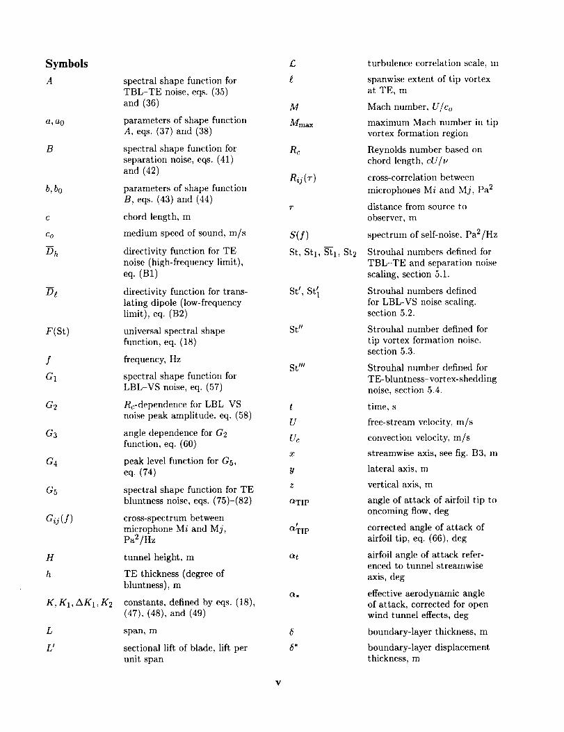
Symbols
A
a, a 0
B
b, b0
c
Co
Dh
D_
F(St)
f
G1
G2
G3
G4
G5
c_j(f)
H
h
K, K1, AK1, K2
L
L I
spectral shape function for
TBL-TE noise, eqs. (35)
and (36)
parameters of shape function
A, eqs. (37) and (38)
spectral shape function for
separation noise, eqs. (41)
and (42)
parameters of shape function
B, eqs. (43) and (44)
chord length, m
medium speed of sound, m/s
directivity function for TE
noise (high-frequency limit),
eq. (B1)
directivity function for trans-
lating dipole (low-frequency
limit), eq. (B2)
universal spectral shape
function, eq. (18)
frequency, Hz
spectral shape function forLBL VS noise, eq. (57)
Rc-dependence for LBL VS
noise peak amplitude, eq. (58)
angle dependence for G2
function, eq. (60)
peak level function for G5,
eq. (74)
spectral shape function for TEbluntness noise, eqs. (75)-(82)
cross-spectrum between
microphone Mi and M j,
pa2/Hz
tunnel height, m
TE thickness (degree of
bluntness), m
constants, defined by eqs. (18),
(47), (48), and (49)
span, m
sectional lift of blade, lift per
unit span
£
M
Mmax
Rc
Rij(r)
s(f)
St, Stl, Stl, St2
St l, St_
St"
St m
t
U
u_
x
Y
z
C_TIP
aTIP
g_t
Og,
6*
v
turbulence correlation scale, m
spanwise extent of tip vortexat TE, m
Mach number, U/co
maximum Mach number in tip
vortex formation region
Reynolds number based on
chord length, cU/u
cross-correlation between
microphones Mi and M j, Pa 2
distance from source to
observer, m
spectrum of self-noise, Pa2/Hz
Strouhal numbers defined for
TBL--TE and separation noise
scaling, section 5.1.
Strouhal numbers defined
for LBL-VS noise scaling,section 5.2.
Strouhal number defined for
tip vortex formation noise,section 5.3.
Strouhal number defined for
TE-bluntness vortex-shedding
noise, section 5.4.
time, s
free-stream velocity, m/s
convection velocity, m/s
streamwise axis, see fig. B3, m
lateral axis, m
vertical axis, m
angle of attack of airfoil tip tooncoming flow, deg
corrected angle of attack of
airfoil tip, eq. (66), deg
airfoil angle of attack refer-enced to tunnel streamwise
axis, deg
effective aerodynamic angleof attack, corrected for open
wind tunnel effects, deg
boundary-layer thickness, m
boundary-layer displacement
thickness, m

F
O
T
¢
Subscripts:
avg
e
P
8
TIP
TOT
Ot
tip vortex strength, m2/s
angle from source streamwise
axis x to observer, see fig. B3,deg
boundary-layer momentum
thickness, m
kinematic viscosity of medium,
m2/s
time delay, s
angle from source lateral axis y
to observer, see fig. B3, deg
cross-spectral phase angle, deg
angle parameter related to sur-
face slope at TE, section 5.4,deg
average
retarded coordinate
pressure side of airfoil
suction side of airfoil
tip of blade
total
angle dependent
1/3
Abbreviations:
BL
LBL
LE
LHS
Mi
OASPL
RHS
SPL
TBL
TE
UTRC
VS
2D
3D
for b0, _, and 00 is for airfoilat zero angle of attack, refer-ence value
1/3-octave spectral
presentation
boundary layer
laminar boundary layer
leading edge of airfoil blade
left-hand side
microphone number i for i -- 1
through 9, see fig. 4
overall sound pressure level,dB
right-hand side
sound pressure level, spectrum,
dB (re 2 × 10 -5 Pa)
turbulent boundary layer
trailing edge of airfoil blade
United Technologies ResearchCenter
vortex shedding
two-dimensional
three-dimensional
vi

Summary
An overall prediction method has been developed for the self-generated noise
of an airfoil blade encountering smooth flow. Prediction methods for individual
self-noise mechanisms are semiempirical and are based on previous theoretical
studies and the most comprehensive self-noise data set available. The specially
processed data set, most of which is newly presented in this report, is from aseries of aerodynamic and acoustic tests of two- and three-dimensional airfoilblade sections conducted in an anechoic wind tunnel. Five self-noise mecha-
nisms due to specific boundary-layer phenomena have been identified and mod-
eled: boundary-layer turbulence passing the trailing edge, separated-boundary-
layer and stalled-airfoil flow, vortex shedding due to laminar-boundary-layerinstabilities, vortex shedding from blunt trailing edges, and the turbulent vor-
tex flow existing near the tips of lifting blades. The data base, with which the
predictions are matched, is from seven NACA 0012 airfoil blade sections of dif-
ferent sizes (chord lengths from 2.5 to 61 cm) tested at wind tunnel speeds up
to Mach 0.21 (Reynolds number based on chord up to 3 x 10⁶) and at angles of
attack from 0° to 25.2 °. The predictions are compared successfully with pub-
lished data from three self-noise studies of different airfoil shapes, which were
tested up to Mach and Reynolds numbers of 0.5 and 4.6 x 10⁶, respectively.
An application of the prediction method is reported for a large-scale-model he-
licopter rotor and the predictions compared well with data from a broadband
noise test of the rotor, conducted in a large anechoic wind tunnel. A computer
code of the methods is given for the predictions of 1/3-octave formatted spectra.

I. Introduction
Airfoil self-noise is due to the interaction be-
tween an airfoil blade and the turbulence produced
in its own boundary layer and near wake. It is
the total noise produced when an airfoil encounters
smooth nonturbulent inflow. Over the last decade,
research has been conducted at and supported by
NASA Langley Research Center to develop funda-
mental understanding, as well as prediction capabil-
ity, of the various self-noise mechanisms. The interest
has been motivated by its importance to broadband
helicopter rotor, wind turbine, and airframe noises.
The present paper is the cumulative result of a se-
ries of aerodynamic and acoustic wind tunnel tests
of airfoil sections, which has produced a comprehen-
sive data base. A correspondingly extensive semi-empirical scaling effort has produced predictive
capability for five self-noise mechanisms.
1.1. Noise Sources and Background
Previous research efforts (prior to 1983) for thebroadband noise mechanisms are reviewed in some
detail by Brooks and Schlinker (ref. 1). In fig-
ure 1, the subsonic flow conditions for five self-noise
mechanisms of concern here are illustrated. At high
Reynolds number Rc (based on chord length), turbu-
lent boundary layers (TBL) develop over most of the
airfoil. Noise is produced as this turbulence passes
over the trailing edge (TE). At low Rc, largely lam-
inar boundary layers (LBL) develop, whose instabil-
ities result in vortex shedding (VS) and associated
noise from the TE. For nonzero angles of attack, the
flow can separate near the TE on the suction side of
the airfoil to produce TE noise due to the shed tur-bulent vorticity. At very high angles of attack, the
'separated flow near the TE gives way to large-scale
separation (deep stall) causing the airfoil to radiate
low-frequency noise similar to t,hat of a bluff body in
flow. Another noise source is vortex shedding occur-
ring in the small separated flow region aft of a blunt
TE. The remaining source considered here is due to
the formation of the tip vortex, containing highly tur-
bulent flow, occurring near the tips of lifting bladesor wings.
1.1.1. Turbulent-Boundary-Layer-Trailing-Edge
(TBL TE) Noise
Using measured surface pressures, Brooks and
Hodgson (ref. 2) demonstrated that if sufficient infor-
mation is known about the TBL convecting surface
pressure field passing the TE, then TBL-TE noisecan be accurately predicted. Schlinker and Amiet
(ref. 3) employed a generalized empirical description
of surface pressure to predict measured noise. How-
ever, the lack of agreement for many cases indicated
2
_W Turbulent ..
ake
Turbulent-boundary-layermtrailing-edgenoise
_Laminar r- Vortex
undary layering
waves
Laminar-boundary-layer--vortex-sheddingnoise
V Boundary-layer
Large-scale separation(deep stall)
Separation-stall noase
_Blunt trailing edge\
Trailing-edge-bluntness--vortex-sheddingnoise
Tip vortex
Tip vortex formation noise
Figure 1. Flow conditions producing airfoil blade self-noise.

a needfor amoreaccuratepressuredescriptionthanwasavailable.Langleysupporteda researcheffort(ref.4) to modeltheturbulencewithinboundarylay-ersasasumofdiscrete"hairpin"vortexelements.Ina paralleland follow-upeffort, the presentauthorsmatchedmeasuredand calculatedmeanboundary-layercharacteristicsto prescribeddistributionsofthediscretevortexelementssothat associatedsurfacepressurecouldbedetermined.Theuseof themodelto predictTBL TE noiseproveddisappointingbe-causeof its inabilityto showcorrecttrendswith an-gleof attackor velocity.Theresultsshowedthat tosuccessfullydescribethesurfacepressure,thehistoryof theturbulencemustbeaccountedfor in additionto the meanTBL characteristics.This levelof tur-bulencemodelinghasnot beenattemptedto date.
A simplerapproachto the TBL TE noiseprob-lemisbasedon the Ffowcs Williams and Hall (ref. 5)
edge-scatter formulation. In reference 3, the noise
data were normalized by employing the edge-scattermodel with the mean TBL thickness 5 used as a
required length scale. When 5 was unknown, sim-
ple flat plate theory was used to estimate 5. Spec-
tral data initially differing by 40 dB collapsed to
within 7 dB, consistent with the results of the ap-
proach discussed above using surface pressure mod-
els. The extent of agreement between data sets was
largely due to the correct scaling of the velocity de-
pendence, which is the most sensitive parameter in
the scaling approach. The dependence of the overall
sound pressure level on velocity to the fifth powerhad been verified in a number of studies. The ex-
tent to which the normalized data deviation was due
to uncertainty in 5 was addressed by Brooks and
Marcolini (ref. 6) in a forerunner to the present re-
port. For large Rc and small angles of attack, which
matched the conditions of reference 3, the use of mea-
sured TBL thicknesses 5, displacement thicknesses
5", or momentum thicknesses/_ in the normalization
produced the same degree of deviation within theTBL TE noise data. Subsequently, normalizations
based on boundary-layer maximum shear stress mea-
surements and, alternately, profile shape factors were
also examined. Of particular concern in reference 6
was that when an array of model sizes, rather than
just large models, was tested at various angles of at-
tack, the normalized spectrum deviations increased
to 10 or even 20 dB. These large deviations indicate
a lack of fidelity of the spectrum normalization and
any subsequent prediction methods based on curvefits. They also reinforce the conclusion from the
aforementioned surface pressure modeling effort that
knowledge of the mean TBL characteristics alone isinsufficient to define the turbulence structure. The
conditions under which the turbulence evolves were
found to be important. The normalized data ap-
peared to be directly influenced by factors such as
Reynolds number and angle of attack, which in pre-vious analyses were assumed to be of pertinence only
through their effect on TBL thickness 6 (refs. 3 and7).
Several prediction schemes for TBL TE noise
have been used previously for helicopter rotor noise
(refs. 3 and 8) and for wind turbines (refs. 9 and
10). These schemes have all evolved from scaling lawequations which were fitted to the normalized data
of reference 3 and, thus, are limited by the same con-
cerns of generality discussed above.
1.1.2. Separation-Stall Noise
Assessments of the separated flow noise mecha-
nism for airfoils at moderate to high angles of at-
tack have been very limited (ref. 1). The relative
importance of airfoil stall noise was illustrated ill
the data of Fink and Bailey (ref. 11) in an airframe
noise study. At stall, noise increased by more than10 dB relative to TBL TE noise, emitted at low an-
gles of attack. Paterson et al. (ref. 12) found evidencethrough surface to far field cross-correlations that for
mildly separated flow the dominant noise is emitted
from the TE, whereas for deep stall the noise radiated
from the chord as a whole. This finding is consistentwith the conclusions of reference 11.
No predictive methods are known to have been
developed. A successful method would have to ac-
count for the gradual introduction of separated flow
noise as airfoil angle of attack is increased. Beyond
limiting angles, deep stall noise would be the only
major contributing source.
1.1.3. Laminar-Boundary-Layer Vortex-
Shedding (LBL VS) Noise
When a LBL exists over most of at least one
side of an airfoil, vortex shedding noise can oc-
cur. The vortex shedding is apparently coupledto acoustically excited aerodynamic feedback loops
(refs. 13, 14, and 15). In references 14 and 15, the
feedback loop is taken between the airfoil TE and
an upstream "source" point on the surface, where
Tollmien-Schlichting instability waves originate in
the LBL. The resulting noise spectrum is composed
of quasi-tones related to the shedding rates at theTE. The gross trend of the frequency dependence
was found by Paterson et al. (ref. 16) by scaling on aStrouhal number basis with the LBL thickness at the
TE being the relevant length scale. Simple fiat plate
LBL theory was used to determine the boundary-
layer thicknesses 5 in the frequency comparisons.The use of measured values of 5 in reference 6 veri-
fied the general Strouhal dependence. Additionally,
3

forzeroangleofattack,BrooksandMarcolini(ref.6)foundthat overalllevelsof LBL VS noisecouldbenormalizedsothat thetransitionfromLBL VSnoiseto TBL TE noiseis auniquefunctionof Rc.
There have been no LBL VS noise prediction
methods proposed, because most studies have em-
phasized the examination of the rather erratic fre-
quency dependence of the individual quasi-tones in
attempts to explain the basic mechanism. However,
the scaling successes described above in references 6
and 16 can offer initial scaling guidance for the de-
velopment of predictions in spite of the general com-
plexity of the mechanism.
1.1.3. Tip Vortex Formation Noise
The tip noise source has been identified with the
turbulence in the local separated flow associated with
formation of the tip vortex (ref. 17). The flow over
the blade tip consists of a vortex with a thick viscous
turbulent core. The mechanism for noise production
is taken to be TE noise due to the passage of the
turbulence over the TE of the tip region. George and
Chou (ref. 8) proposed a prediction model based on
spectral data from delta wing studies (assumed to
approximate the tip vortex flow of interest), meanflow studies of several tip shapes, and TE noise
analysis.
Brooks and Marcolini (ref. 18) conducted an ex-
perimental study to isolate tip noise in a quantitative
manner. The data were obtained by comparing setsof two- and three-dimensional test results for differ-
ent model sizes, angles of attack, and tunnel flow ve-
locities. From data scaling, a quantitative prediction
method was proposed which had basic consistencywith the method of reference 8.
1.1.5. Trailing-Edge-Bluntness Vortex-SheddingNoise
Noise due to vortex shedding from blunt trailing
edges was established by Brooks and Hodgson (ref. 2)to be an important airfoil self-noise source. Other
studies of bluntness effects, as reviewed by Blake
(ref. 19) and Brooks and Schlinker (ref. 1), were onlyaerodynamic in scope and dealt with TE thicknesses
that were large compared with the boundary-layer
displacement thicknesses. For rotor blade and wing
designs, the bluntness is likely to be small comparedwith boundary-layer thicknesses.
Grosveld (ref. 9) used the data of reference 2 to
obtain a scaling law for TE bluntness noise. He found
that the scaling model could explain the spectralbehavior of high-frequency broadband noise of wind
turbines. Chou and George (ref. 20) followed suitwith an alternative scaling of the data of reference 2
to model the noise. For both modeling techniques
neither the functional dependence of the noise on
boundary-layer thickness (as compared with the TE
bluntness) nor the specifics of the blunted TE shape
were incorporated. A more general model is needed.
1.2. Overview of Report
The purpose of this report is to document the de-
velopment of a self-noise prediction method and to
verify its accuracy for a range of applications. The
tests producing the data base for the scaling effortare described in section 2. In section 3, the mea-
sured boundary-layer thickness and integral parame-
ter data, used to normalize airfoil noise data, are doc-
umented. The acoustic measurements are reported in
section 4, where a special correlation editing proce-dure is used to extract clean self-noise spectra from
data containing extraneous test rig noise. In sec-
tion 5, the scaling laws are developed for the five self-
noise mechanisms. For each, the data are first nor-
malized by fundamental techniques and then exam-
ined for dependences on parameters such as Reynolds
number, Mach number, and geometry. The resultingprediction methods are delineated with specific calcu-
lation procedures and results are compared with the
original data base. The predictions are compared insection 6 with self-noise data from three studies re-
ported in the literature. In appendix A, the data
processing technique is detailed; in appendix B, the
noise directivity functions are defined; and in appen-dix C, an application of the prediction methods is re-
ported for a helicopter rotor broadband noise study.
In appendix D, a computer code of the predictionmethod is given.

2. Description of Experiments
The details of the measurements and test facil-
ity have been reported in reference 6 for the sharpTE two-dimensional (2D) airfoil model tests, in ref-
erence 18 for corresponding three-dimensional (3D)tests, and in reference 2 for the blunt TE 2D airfoil
model test. Specific information applicable to thisreport is presented here.
2.1. Models and Facility
The models were tested in the low-turbulence po-tential core of a free jet located in an anechoic cham-
ber. The jet was provided by a vertically mounted
nozzle with a rectangular exit with dimensions of
30.48 × 45.72 cm. The 2D sharp TE models are
shown in figure 2. The models, all of 45.72-cm span,
were NACA 0012 airfoils with chord lengths of 2.54,5.08, 10.16, 15.24, 22.86, and 30.48 cm. The models
were made with very sharp TE, less than 0.05 mm
thick, without beveling the edge. The slope of the
surface near the uncusped TE corresponded to therequired 7 ° off the chord line. The sharp TE 3D mod-
els, shown in figure 3, all had spans of 30.48 cm and
chord lengths that were the same as the five largest2D models. The 3D models had rounded tips, defined
by rotating the NACA 0012 shape about the chord
line at 30.48-cm span. An NACA 0012 model of per-
tinence to the present paper, which is not shown here,
is the blunt-TE airfoil of reference 2, with a chordlength of 60.96 cm. Details of the blunt TE of this
large model are given in section 5.The cylindrical hubs, shown attached to the mod-
els, provided support and flush-mounting on the side
plates of the test rig. At a geometric tunnel angleof attack o_t of 0°, the TE of all models was located
61.0 cm above the nozzle exit. The tunnel angle at isreferenced to the undisturbed tunnel streamline di-
rection. In figure 4, an acoustic test configuration for
a 3D model is shown. A 3D setup is shown so that
the model can be seen fitted to the side plate. The
side plates (152.4 x 30.0 x 1 cm) were reinforcedand flush mounted on the nozzle lips. For the 2D
configurations, an additional side plate was used.
2.2. Instrumentation
For all of the acoustic testing, eight 1.27-cm-
diameter (1/2-in.) free-field-response microphones
were mounted in the plane perpendicular to the 2D
model midspan. One microphone was offset from
this midspan plane. In figure 4, seven of theseare shown with the identification numbers indicated.
Microphones M1 and M2 were perpendicular to thechord line at the TE for at = 0 °. The other
microphones shown were at radii of 122 cm from
the TE, as with M1 and M2, but were positioned
30 ° forward (M4 and M7) and 30 ° aft (M5 and M8).
The data acquisition and processing approaches aredescribed in appendix A.
For the aerodynamic tests the microphones to
the right in figure 4 were removed and replaced by
a large three-axis computer-controlled traverse rigused to position hot-wire probes. The miniature
probes included both cross-wire and single-wire con-figurations. In figure 5, a cross-wire probe is shown
mounted on the variable-angle arm of the traverse rig.Again, for clarity, a 3D airfoil model is shown. The
probes were used to survey the flow fields about the
models, especially in the boundary-layer and near-
wake region just downstream of the trailing edge.
2.3. Test Conditions
The models were tested at free-stream velocities
U up to 71.3 m/s, corresponding to Mach num-
bers up to 0.208 and Reynolds numbers, based oil a
30.48-cm-chord model, up to 1.5 x 10⁶. The tunnel
angles of attack c_t were 0°, 5.4 °, 10.8 °, 14.4 °, 19.8 °,
and 25.2 ° . The larger angles were not attemptedfor the larger models to avoid large uncorrectabletunnel flow deflections. For the 22.86-cra- and
30.48-cm-chord models, (_t was limited to 19.8 ° and
14.4 ° , respectively.
For the untripped BL cases (natural BL develop-
ment), the surfaces were smooth and clean. For the
tripped BL cases, BL transition was achieved by a
random distribution of grit in strips from the lead-
ing edge (LE) to 20 percent chord. This tripping
is considered heavy because the chordwise extent ofthe strip produced thicker than normal BL thick-
nesses. It was used to establish a well-developedTBL even for the smaller models and at the same
time retain geometric similarity. The commercial
grit number was No. 60 (nominal particle diam-
eter of 0.29 mm) with an application density of
about 380 particles/cm 2. An exception was the
2.54-cm-chord airfoil which had a strip at 30 per-
cent chord of No. 100 grit with a density of about690 particles/era 2.
2.4. Wind Tunnel Corrections
The testing of airfoil models in a finite-size openwind tunnel causes flow curvature and downwash
deflection of the incident flow that do not occur in
free air. This effectively reduces the angle of attack,
more so for the larger models. Brooks, Marcolini, and
Pope (ref. 21) used lifting surface theory to develop
the 213 open wind tunnel corrections to angle ofattack and camber. Of interest here is a corrected
angle of attack _, representing the angle in free air
required to give the same lift as at would give in the
tunnel. One has from reference 21, upon ignoring
5

Figure 2. Two-dimensional NACA 0012 airfoil blade models.
L-82-4573
6
Figure 3. Three-dimensional NACA 0012 airfoil blade models.
L-82-4570
ORIGINAL PAG1E
BLACK AND WHITE PHOTOGRAPH

OR!_qTN_L"P_CE'Rt ,_ ....
.... ,C_ A;",O WHITE PHOTOCR/_,pH
MicrophoneM2
Figure 4. Test setup for acoustic tests of a 3D model airfoil.
L-89-42
Traverse arm
Hot-wire probe
Trailing edgeSide plate
3D airfoil model
Figure 5. Tip survey using hot-wire probe.
L-89-43

small camber effects,
where
and
a, --- _t/_
= (1 + 2a) 2 +
a = (r2/48)(c/H) 2
(1)
The term c is the airfoil chord and H is the tunnel
height or vertical open jet dimension for a horizon-
tally aligned airfoil. For the present 2D configura-
tions, a./at equals 0.88, 0.78, 0.62, 0.50, 0.37, and0.28 for the models with chord lengths of 2.54, 5.08,
10.16, 15.24, 22.86, and 30.48 cm, respectively.
8
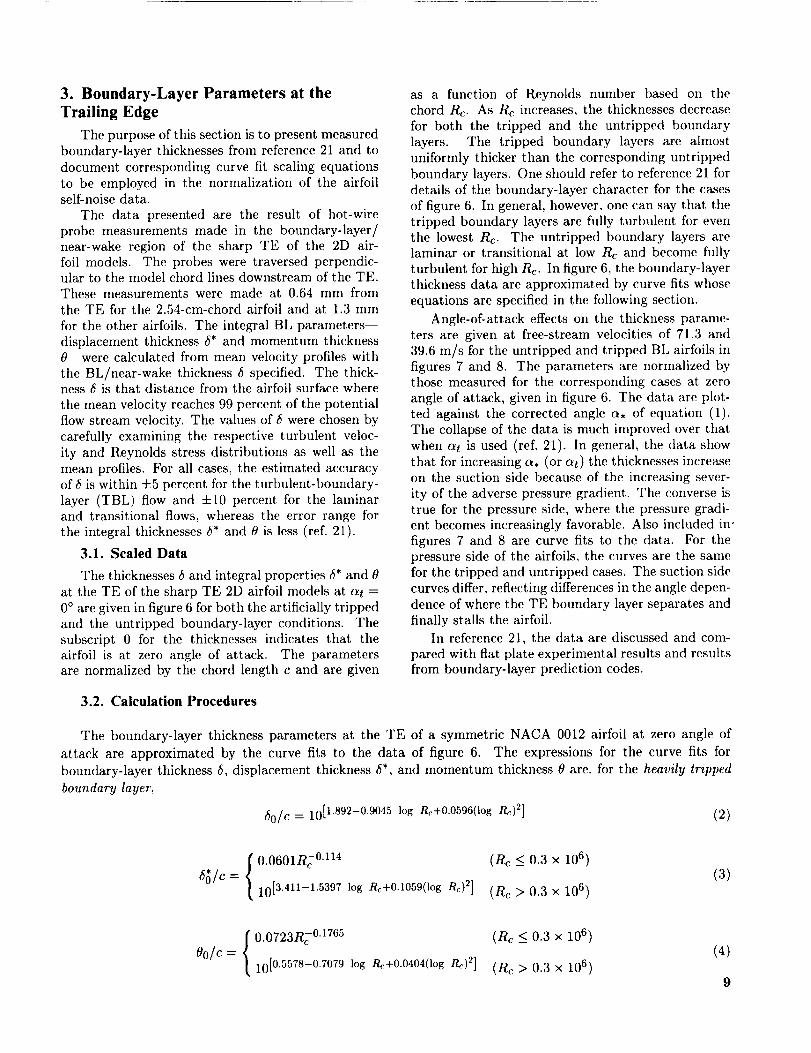
3. Boundary-Layer Parameters at the
Trailing Edge
The purpose of this section is to present measured
boundary-layer thicknesses from reference 21 and to
document corresponding curve fit scaling equations
to be employed in the normalization of the airfoilself-noise data.
The data presented are the result of hot-wire
probe measurements made in the boundary-layer/
near-wake region of the sharp TE of the 2D air-foil models. The probes were traversed perpendic-ular to the model chord lines downstream of the TE.
These measurements were made at 0.64 mm from
the TE for the 2.54-cm-chord airfoil and at 1.3 mm
for the other airfoils. The integral BL parameters--
displacement thickness 5' and momentum thickness0 were calculated from mean velocity profiles with
the BL/near-wake thickness 5 specified. The thick-ness 5 is that distance from the airfoil surface where
the mean velocity reaches 99 percent of the potentialflow stream velocity. The values of 6 were chosen by
carefully examining the respective turbulent veloc-
ity and Reynolds stress distributions as well as the
mean profiles. For all cases, the estimated accuracy
of 6 is within ±5 percent for the turbulent-boundary-
layer (TBL) flow and +10 percent for the laminarand transitional flows, whereas the error range for
the integral thicknesses 5* and 0 is less (ref. 21).
3.1. Scaled Data
The thicknesses 6 and integral properties 6" and 0
at the TE of the sharp TE 2D airfoil models at st =
0° are given in figure 6 for both the artificially trippedand the untripped boundary-layer conditions. The
subscript 0 for the thicknesses indicates that theairfoil is at zero angle of attack. The parameters
are normalized by the chord length c and are given
as a function of Reynolds number based ou the
chord Rc. As Rc increases, the thicknesses decrease
for both the tripped and the untripped boundary
layers. The tripped boundary layers are almost
uniformly thicker than the corresponding untripped
boundary layers. One should refer to reference 21 for
details of the boundary-layer character for the cases
of figure 6. In general, however, one can say that the
tripped boundary layers are fully turbulent for even
the lowest Rc. The untripped boundary layers arelaminar or transitional at low Rc and become fully
turbulent for high Rc. In figure 6, the boundary-layerthickness data are approximated by curve fits whose
equations are specified in the following section.
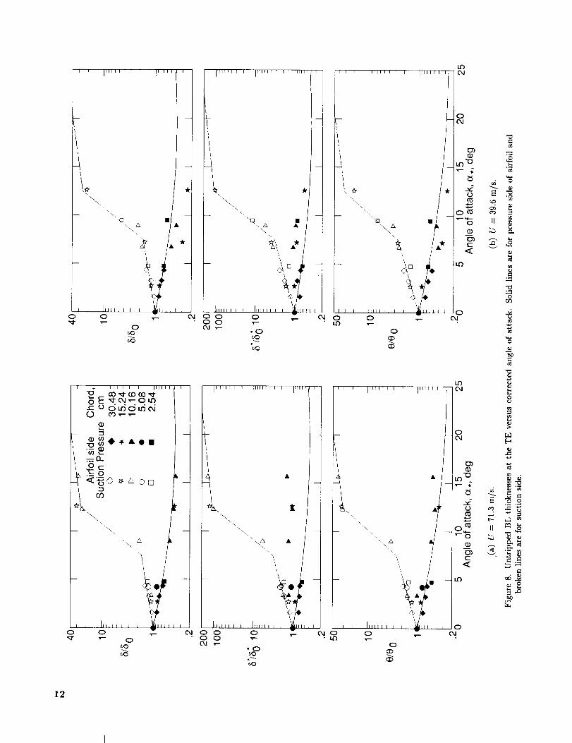
Angle-of-attack effects on the thickness parame-
ters are given at free-stream velocities of 71.3 and
39.6 m/s for the untripped and tripped BL airfoils infigures 7 and 8. The parameters are normalized by
those measured for the corresponding cases at zero
angle of attack, given in figure 6. The data are plot-
ted against the corrected angle (_, of equation (1).
The collapse of the data is much improved over that
when st is used (ref. 21). In general, the data show
that for increasing c_, (or c_t) the thicknesses increaseon the suction side because of the increasing sever-
ity of the adverse pressure gradient. The converse istrue for the pressure side, where the pressure gradi-
ent becomes increasingly favorable. Also included in"
figures 7 and 8 are curve fits to the data. For the
pressure side of the airfoils, the curves are the same
for the tripped and untripped cases. The suction side
curves differ, reflecting differences in the angle depen-dence of where the TE boundary layer separates and
finally stalls the airfoil.
In reference 21, the data are discussed and com-
pared with flat plate experimental results and results
from boundary-layer prediction codes.
3.2. Calculation Procedures
The boundary-layer thickness parameters at the TE of a symmetric NACA 0012 airfoil at zero angle of
attack are approximated by the curve fits to the data of figure 6. The expressions for the curve fits for
boundary-layer thickness 5, displacement thickness 5", and momentum thickness 0 are, for the heavily tripped
boundary layer,
50/c = 1011.892-0.9045 log Re+0.0596(log R_) 2] (2)
0.0601Re 0"114
1013.411-1.5397 log nc+0.1059(log Re) 2]
(Re < 0.3 x 10⁶)
(Rc>O.3x 106 )
(3)
0.0723Rc .1765O0/c ---- 1010.5578_0.7079 log P,w+0.0404(log Re) 2]
(Rc < 0.3 x 10⁶)(4)
(Rc > 0.3 x 10⁶ )9

Boundary layer Airfoil chord,Tripped Untripped cm
© • 30.48. 15.24• 10.16
O • 5.08[] • 2.54
80/c
.01
1-4
J L I I I I I _ I t I I _ J I
86/c
.001
.02
.01
e0/c
i i n i i I i , J i I _ I r I
' ' ' ' ' I ........ I
: ..... _---_-_a_O O
• • _- .... -_.
.001 J I I Ill J 1 I [ J J J L l '.04 .1 1 3 X 10 6
Reynolds number, Rc
Figure 6. Boundary-layer thicknesses at the trailing edge of 2D airfoil models at angle of attack of zero. Solid lines are for
untripped BL and broken lines are for tripped BL.
10

ou"XI
oOd
iflll [ i I
0
IllJJ I i J I
o
o
lllll
o
' I....t , j
"I
/
r
r i [ I [ITI[ I l
d_d_N_r
i 0@_-=_0_
.__o
' Ct
o
IIILI L I J
or
O_SOL_
I II
I 111 } I I
0 r-
L-
't
j[lll I I I I I[IIfTTI I
Ilr
jJILI I i i t _ II I _
0 ,,--
r "0
co
_ n •\
"_ _ I' I -
• If)0 -,- 0,I 0r '0 • Cn,l
_o
Illlll I I [
--_I 0
ik
-- \
\
IIl_l I I I
or-
111111 I
\
o
I..O
o
i
_,.+---_ 0
C
o
_4
II
d
II
0
..,4
8
kt-.1
= d
_.o
11
_ ' I ...... i, I....
-4
\
\
I I III] _ L J i
0 0
',,--0
_O
I I Ill_li J I
0 0
co
T . ]111 I I I Ili111
I oE _,-o_
T--
I I
m
TTIIII _ I
4I
\
\\
I I
0
U3
IIITII; I I IIII1[1 I I
4I
\I-- \_.
\
\
IHIIT 1
m
k
m
IIIIII I I T IIIIIT I
\
,.\
\ A.
\\
I l_llll i I
0
0
IITll f I I 1
\
\
0
0
\
I°,,I _l_l_lt I I l 0
•,-- 04
' Od
loi°
LO"_
o_
<_
0r,/)
,.=
",.0
Cb
12

wherethezerosubscriptsindicatezeroangleof attack,zerolift on thesesymmetricairfoils.Forthe untripped
(natural transition) boundary layers,
60/C = 1011.6569-0.9045 log Rc+0.0596(log Re) 2] (5)
_/e = 10 [3'0187-1'5397 log Rc+0.1059(log Re) 2] (6)
O0/e = 1010.2021-0.7079 log Rc+0.040a(log p_)2] (7)
The boundary-layer thicknesses for the airfoils at nonzero angle of attack, in terms of the zero-angle-of-
attack thicknesses and the corrected angles o_,, are given in figures 7 and 8. The expressions for the curve fits
for the pressure side, for both the tripped and the untripped boundary layers, are
6p _-- 10[_0.04175a,+0.00106o_,2 ] (8)60
P ---- 10[ -0'0432°_*+0"00113a.2] (9)
0p = 10[_0.04508a,+0.000873a,2 ] (10)00
For the suction side, the parametric behavior of the thicknesses depends on whether the boundary layers are
attached, separated near the trailing edge, or separated a sufficient distance upstream to produce stall. For
the suction side for the tripped boundary layers (fig. 7),
6s [ lO0"0311a* (0° -< or, _< 5°)
_0 = / 0"3468(100"1231'_*) (50 < o_, < 12.5 °)5.718(100"0258a*) (12.5 ° < o_, < 25 °)
(11)
{ 100.0679c_,6__= 0.3s1(100.1516-,)
6_ 14.296(100"0258a*)
(0° < a, < 5o)
(5 ° <a, < 12.5 ° )
(12.5 ° < a, < 25 ° )
(12)
Os { 100"0559c_*_00 = 0.6984( 100'0869a' )
4.0846(10 °'°258a*)
(0° < _, < 5°)
(5 °<a,<12.5 ° )
(12.5 ° < o_, _< 25 °)
(13)
13

Forthe suction side for the untripped boundary layers (fig. 8),
100.03114a,5s = 0.0303(1002336_*
60 12( I00"0258_" )
(0 ° < a, < 7.5 °
(7.5 ° < a, < 12.5 °
(12.5 ° < a, < 25 °
100.0679a*6._ = 0.0162(100.3066c_,
6_ 52.42(100"°258_* )
100.0559a*Os = 0.0633(100.2157_,Oo
14.977(10 °'°25s_*
(0 ° < a, < 7.5 °
(7.5 ° < c_, _< 12.5 °
(12.5 ° < a, < 25 °
(0 ° < a, _< 7.5 °
(7.5 ° < or, < 12.5 °
(12.5 ° < c_, < 25 °
(14)
(15)
(16)
14

4. Acoustic Measurements
The aim of the acoustic measurements was to de-
termine spectra for self-noise from airfoils encoun-
tering smooth airflow. This task is complicated by
the unavoidable presence of extraneous tunnel test
rig noise. In this section, cross-correlations between
microphones are examined to identify the self-noiseemitted from the TE in the presence of other sources.
Then, the spectra of self-noise are determined by per-
forming Fourier transforms of cross-correlation data
which have been processed and edited to eliminate
tile extraneous contributions. The results are pre-
sented as 1/3-octave spectra, which then form the
data base from which the self-noise scaling predic-
tion equations are developed.
4.1. Source Identification
The upper curves in figure 9 are the cross-
correlations, R12(r) = (pl(t)p2(t + r)}, between the
sound pressure signals Pl and P2 of microphones M1
and M2 identified in figure 4. Presented are cross-
correlations both with and without the tripped 30.48-
cm-chord airfoil mounted in the test rig. Because the
microphones were on opposite sides of, and at equal
distance from, the airfoil, a negative correlation peak
occurs at a signal delay time T of 0. This correlation
is consistent with a broadband noise source of dipolecharacter, whose phase is reversed on opposing sides.
When the airfoil is removed, the strong negative peak
disappears leaving the contribution from the test rig
alone. The most coherent parts of this noise are from
the lips of the nozzle and are, as with the airfoil noise,
of a dipole character. The microphone time delays
predicted for these sources are indicated by arrows.
The predictions account for the effect of refraction of
sound by the free-jet shear layer (refs. 22 and 23), as
well as the geometric relationship between the micro-phones and the hardware and the speed of sound.
The lower curves in figure 9 are the cross-
correlations, R45(7-), between microphones M4 and
M5. The predicted delay times again appear to cor-
rectly identify the correlation peaks associated with
the noise emission locations. The peaks are positive
for R45(T) because both microphones are on the same
side of the dipoles' directional lobes. The noise field
is dominated by TE noise. Any contribution to thenoise field from the LE would appear where indicated
in the figure. As is subsequently shown, there are
contributions in many cases. For such cases the neg-
ative correlation peak for R12(r) would be the sum
of the TE and LE correlation peaks brought together
at _- = 0 and inverted in sign.
In figure 10, the cross-correlations R45(T) are
shown for tripped BL airfoils of various sizes. The
TE noise correlation peaks are at TTE = --0.11 ms
for all cases because at at = 0 °, the TE location
of all models is the same. The LE location changeswith chord size, as is indicated by the change in the
predicted LE noise correlation peak delay times.
For the larger airfoils in figure 10, the TE con-tribution dominates the noise field. As the chord
length decreases, the LE noise peaks increase to be-
come readily identifiable in the correlation. For thesmallest chord the LE contribution is even some-
what more than that of the TE. Note the extraneous,
but inconsequential, source of discrete low-frequency
noise contributing to the 22.86-era-chord correlation,
which can be readily edited in a spectral format.It is shown in reference 6 that the LE and TE
sources are uncorrelated. The origin of LE noise
appears to be inflow turbulence to the LE from the
TBL of the test rig side plates. This should be the
ease even though the spanwise extent of this TBL
is small compared with the portion of the modelsthat encounter uniform low-turbulence flow from the
nozzle. Inflow turbulence can be a very efficient
noise mechanism (ref. 24); however its fldl efficiency
can be obtained only when the LE of the model
is relatively sharp compared with the scale of theturbulence. The LE noise contributions diminish for
the large chord because of the proportional increasein LE radius with chord. When this radius increases
to a size that is large compared with the turbulent"
scale in the side plate TBL, then the sectional liftfluctuations associated with inflow turbulence noise
are not developed.
4.2. Correlation Editing and SpectralDetermination
The cross-spectrum between nficrophones M1 andM2, denoted G12(f), is the Fourier transform of
R12(r). If the contributions from the LE, nozzle lips,
and any other coherent extraneous source locations
were removed, G12(f) would equal the autospectrum
of the airfoil TE self-noise, S(f). Actually the rela-
tionship would be G12(f) = S(f)exp[i(21rfrTE =t=7r)],where i = v/-Z1 and TTE is the delay time of the TE
correlation peak. This approach is formalized in ref-erence 2.
In reference 6, the spectra were found from G12(f)
determined with the models of the test rig after a
point-by-point vectorial subtraction of Gl2(f) deter-
mined with the airfoil removed. This was equivalent
to subtracting corresponding R12(T) results, such as
those of figure 9, and then taking the Fourier trans-
form. This resulted in "corrected" spectra which
were devoid of at least a portion of the background
test rig noise, primarily emitted from the nozzle lips.
The spectra still were contaminated by the LE noisedue to the inflow turbulence.
15

.005 .... i .... i .... I '
R12 ('c),
pa2
.OO5
R45 0pa 2
Nozzle Nozzle ' '
liP _ lip I
...... Test rig without
airfoil TEl l A rfo I -
A ,F%z,e%z,e
0052 .... _ .... I .... I ....-' -1 0 1Delay time, "c,ms
2
Figure 9. Cross-correlations for two microphone pairs with and without airfoil mounted in test rig.
c = 30.48 cm; BL tripped; at = 0°; U = 71.3 m/s. Arrows indicate predicted values of r. (From ref. 6.)
.005
0
.005
oi
.005
0
.005
0
.005
0
.005
0
' ' ' ' I ' ' ' ' i , , , , I ' ' ' "7Chord length, TE t
cm _ LE 4
22.86 1 -
TE l LE
TEj LE
TE ILE
2.54 _
-.005 ..... I .... i .... _ ....-2 -1 0 1
Delay time,z, ms
Figure 10. Cross-correlations between microphones M4 and M5 for tripped BL airfoils of various chord sizes. U = 71.3 m/s.
Arrows indicate predicted values of r. (From ref. 6.)
16

In the present paper, most spectra presentedwere obtained by taking the Fourier transform of
microphone-pair cross-correlations which had been
edited to eliminate LE noise (see details in appen-
dix A). The microphone pairs used included M4 andM5, M4 and M8, and M4 and M2. These pairs pro-
duced correlations where the TE and LE noise peaks
were generally separated and readily identifiable. Re-ferring to figure 10 for R45(T), the approach was to
employ only the left-hand side (LHS) of the TE noise
peak. The LHS was "folded" about r at the peak
(7TE) to produce a nearly symmetrical correlation.Care was taken in the processing to maintain the ac-
tual shapes near the very peak, to avoid to the extent
possible the artificial introduction of high-frequency
noise in the resulting spectra. Cross-spectra werethen determined which were equated to the spectraof TE self-noise.
The data processing was straightforward for the
larger chord airfoils because the LE and TE peakswere sufficiently separated from one another that the
influence of the LE did not significantly impact the
TE noise correlation shapes. For many of the smaller
airfoils, such as those with chord lengths of 2.54, 5.08,
and 10.16 cm shown in figure 10, the closeness of theLE contribution distorted the TE noise correlation.
A processing procedure was developed to effectively
"separate" the TE and LE peaks to a sufficient dis-tance from one another, within the correlation pre-
sentation, so that the correlation folding of the LHS
about rTE produced a more accurate presentation ofthe TE noise correlation shape. The separation pro-
cessing employed symmetry assumptions for the TEand LE noise correlations to allow manipulation of
the correlation records. This processing representeda contamination removal method used for about one-
quarter of the spectra presented for tile three small-
est airfoil chord lengths. Each case was treated in-
dividually to determine whether correlation folding
alone, folding after the separation processing, or not
folding at all produced spectra containing the least
apparent error. In appendix A, details of the edit-
ing and Fourier transform procedures, as well as the
separation processing, are given.
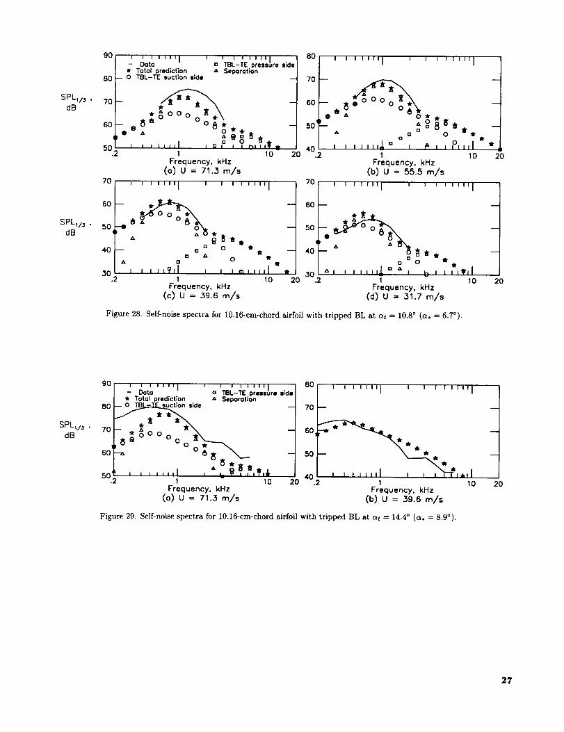
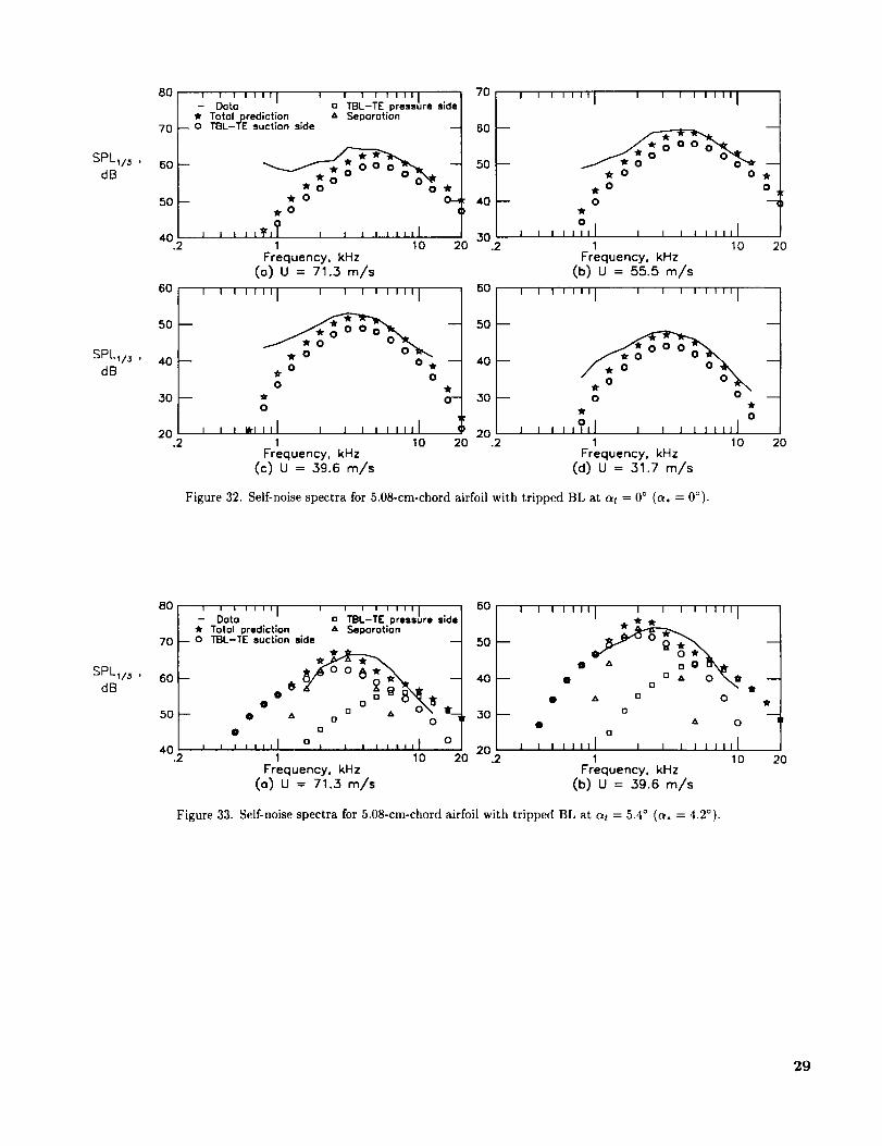
4.3. Self-Noise Spectra
The self-noise spectra for the 2D NACA 0012
airfoil models with sharp TE are presented in a
1/3-octave format in figures 11 to 74. Figures 11to 43 are for airfoils where the boundary layers have
been tripped and figures 44 to 74 are for smooth sur-
face airfoils where the boundary layers are untripped
(natural transition). Each figure contains spectra for
a model at a specific angle of attack for various tun-
nel speeds. Note that the spectra are truncated at
upper and lower frequencies. This editing of the spec-tra was done because, as described in appendix A, a
review of the narrow-band amplitude and phase for
all cases revealed regions where extraneous noise af-fected the spectra in a significant way (2 dB or more).
These regions were removed from the 1/3-octave
presentations.The spectra levels have been corrected for shear
layer diffraction and TE noise directivity effects, as.
detailed in appendix B. The noise should be that for
an observer positioned perpendicular to, and 1.22 m
from, the TE and the model midspan. In terms of the
directivity definitions of appendix B, re = 1.22 m,Oe = 90 ° , and (be = 90 ° • In section 5 (beginning
on p. 51), the character and parametric behavior ofthe self-noise, as well as the predictions which are
compared with the data, are discussed.
17

SPL_/_ ,
dB
SPLI/_ ,
dB
80
70
6O
50 _
40.2
60
50
40
30
20
- Data TBL-TE pressure side* Total prediction A Seporotlon
_ o TBL-TE suction side
W o_r oO
I 0 1
201 10
Frequency, kHz
(o) U = 71.3 m/s
' '''"I ' ' ' '''"I
-- 0
0
I I I I I III I I I I I I III
.2 1 10 20
Frequency, kHz
(c) U = 39.6 m/s
' '''"1 ' ' ' '''"170 i
60-- . _r.
50 "-_oo
40 -- o _'--o
30 t.2
60 L i50
40
30
20.2
, ,,,,,I , , , ,,,,,I1 10
Frequency, kHz
(b) U = 55.5 m/s
' '''"1 ' ' ' '''"1
20
0
-
, ,, .,,.I , , ,, ,,,,Y;.1 10 20
Frequency, kHz
(d) U = 31.7 m/s
Figure 11. Self-noise spectra for 30.48-cm-chord airfoil with tripped BL at st = 0 ° (o, = 0°).
SPLI/_ ,
dB
80
70
60
50 i
40.2
, , i ,,;, I i i i ' ' ;"/ 60- Data o TBL-TE press re side* Total prediction " Separation
-- O TBL-TE suction side -- 50
8 8A A
[] A _ -- 30A W
,,,I , _ , , ,,,,I n] 201 10 20
Frequency, kHz
(o) U = 71.3 m/s
.2
I I I I III I I I I 1 I II1 I
-_ Q Q A
__ A ,, O0 _
o, , ,,,,,i , , , ,,_,,i
I 10 2O
Frequency, kHz
(b) U = 39.6 m/s
Figure 12. Self-noise spectra for 30.48-cm-chord airfoil with tripped BL at (_t = 5.4 ° ((_, = 1.5°) •
18

SPL,/_ ,
dB
SPL1/_ ,
dB
80 J ' '''"1 ' ' ' '''"/- Data [] TB/-TE press re side
* Total prediction " Separation70 -- 0 TBL-TE suction side
60 -
501
n e,,, 8"]
40 2 = 0• 1 10 20
Frequency, kHz
(o) U = 71.3 m/s
6o|, , '''"I ' ' ' '''"I '
50 _ __
401--,, a " _ O a",_. --
Oo"_ _30 o 8
,, 0 8"-"o !
20 i I i i llll , t t t I I]Jl 0 I.2 1 10 20
Frequency, kHz
(c) U = 39.6 m/s
70
60
50=
40
30.2
60
50
40
30
20.2
' ' '''"1 ' ' ' '''"1
A D
A [] [] D A
O
IA 0
0
A
, , , ,,,,I , , , t,,,,lI 10
Frequency, kHz
(b) U = 55.5 m/s
' ' '''"1 ' ' ' '''"1
88--
o
0
20
8
_' 0 0 _ A A _ 00
-- " 0 _[ --0
0
1 10 20Frequency, kHz
(d) U = 31.7 m/s
Figure 13. Self-noise spectra for 30.48-cm-chord airfoil with tripped BL at cq = 10.8 ° (a, = 3.0°).
SPL1/3 ,
dB
80 ' ' ''"I ' ' ' '''"I- Data o TBL-TE pressure side
'Jr Totol prediction A Seporotion
70 --_
ooO°50--, _ o o k. o 0 o_[ '
° o - . "" 0 "_ _.1-40 , i , i i ill i ! , i i ,,tlO l
.2 1 10 20
Frequency, kHz
(o) U = 71.3 m/s
7° i' ''""I ' ' ''""I60
40 8
30 T , i i i iiii t i i i i i
.2 1 10Frequency, kHz
(b) U = 39.6 m/s
Figure 14. Self-noise spectra for 30.48-cm-chord airfoil with tripped BL at at = 14.4 ° (c_, = 4.0°).
20
19

SPLII_ .dB
SPLI/3 ,dB
80
70
60
50
40
30
' ''"'t ' o' ' ''"'!, |- Dora TBL-TE press-re side_r Totol prediction "_ Seporotlon
_ o TBL-TE suction side
• ,o o
_r O50r_ o
}, , ,,,,I I I i , I Illl O$
40.; 1 10 20Frequency, kHz
(o) U = 71.3 m/s
' ' '''"I ' ' ' '''"I
-_ . -o-lt
o
20 i I I I Jill I i i I i ilil.2 1 10 20
Frequency, kHz(c) u = _9.6 m/s
7O
°°t
::T-.2
60
' ' '''"1 ' ' ' '''"1
lito_r
0 _0
0
i i i i iiii i I i i I llil1 10
Frequency, kHz(b) U = 55.5 m/s
' ' '''"1 ' ' ' '''"1
50 --
30 -- o .O _r
T*20 I I I I IIII I I I I I Ill 0
.2 1 10Frequency, kHz
(d) U = 31.7 m/s
Figure 15. Self-noise spectra for 22.86-cm-chord airfoil with tripped BL at at = 0 ° (a, = 0°).
2O
2O
SPLI/_ ,dB
SPLI/3 ,dB
80
70
60
50
I I I I I I I I I 131 I I I Illil I- Dora TBL-TE press re slde* Totol prediction & Seporotion
__ 0 TBL-TE suction side
o [] A 0, a , ,,,_l = , = , ,,,,I 0
40.2 1 10 20Frequency, kHz
(a) U = 71.3 m/s
60 i i i Jill I i , , i lili I
50_ _.e40' o '_ 0 o _
o A z_ 0 o _' A 0 I_
30 -- A o 8-a, 0
A O
20 i i i illil I i I I I Illl.2 1 10 20
Frequency, kHz(c) U = 39.6 m/s
7O
6O
5O
40
30.2
6O
50
40
30
20.2
I I I I I I I I I I I I I I II I
°% oft ,, *o [] ,it
._o & A 0o
, I,,,,I , , 4',,,,,I1 10
Frequency, kHz(b) U = 55.5 m/s
' ' '''"1 ' ' ' '''"1
D
m A A ._o
•, A oI I I ilill t i i , , ii,_
1 10Frequency, kHz
(d) U = 31.7 m/s
Figure 16. Self-noise spectra for 22.86-cm-chord airfoil with tripped BL at at -- 5.4 ° (a, = 2.0°).
2O
20
2O

SPLII3 ,dB
80 ' ' '''''I ' ' ' '''"I 70 ' '''"I ' ' ' '''"II - Data a TBL-TE pressure side I I
| _ Total prediction " Separation70 _ O TBL-TE suction side -- 60
/6o_ 8 8 - 50 []
'°L: ,oo o a - & - O -- & OOo
40 1 ' , , , ,,,,I , , _' ,,,,,I r , , ,,,,,I , , _' ,,,,,I.2 1 10 20 30.2 1 I0 20
Frequency, kHz Frequency, kHz(a) U = 71.3 m/s
60 t I ,,lll I I , I ,llJl I._ '
50 --_ **I A [] O A
40 "--& a n
8t & 0
30 -- 0
20 J , J ,,,,I J _ I , Ill,l.2
I I
t-
O20
mr
O tI
I I II_II =
1 10 1 10 20Frequency, kHz Frequency, kHz
(c) U = 39.6 m/s (d) U = 31.7 m/s
(b) U = 55.5 m/s
60 ' ''"I ' ' ' '''"I
50 - __
30L. u [] ,, o °
A 0
2o , , ,.,,,I , ,.2
Figure 17. Self-noise spectra for 22.86-cm-chord airfoil with tripped BL at at = 10-8 ° (c=, = 4.0°).
SPLI/3 ,dB
80 ' ' ' ''"I ' ' ' ' ''"I I- Data m TBL-TE pressure sidel
Total prediction " Separation I
°o, ooooooOoo _[] A O B 1_" t
, o u ? I r. I I I I I I II I I I I I I II 0
40.2 1 10 20
mr,,,,,I , , , ,,°,_.,Imr.
1 10 20Frequency, kHz Frequency, kHz
(o) U = 71.3 m/s (b) U = 39.6 m/s
70- I , ' ''''I ' ' ' ' ''''I
so?a .=o_ *.
o a ° & 0 0 "u
[]
30 -_ = J.2
Figure 18. Self-noise spectra for 22.86-cm-chord airfoil with tripped BL at at = 14.4 ° (a, = 5.3°).
21
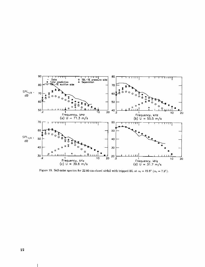
SPLv3 ,
dB
SPLI/_ ,dB
70
60
50
40
30.2
90 ' ' ' ''"I ' ' ' ' ''"II - DoLo o TBL-TE pressure sl
'_ Total prediction & Se oration80 Conside
5 _ , i@,lu.2 1 10 20
Frequency. kHz(o) U = 71.3 m/s
' ' '''"1 ' ' ' '''"1
-80002, _
n o A° °o_i._.-- o [] o "0 "_ik t
[]
P io 11,
J ,IJll _ , , ,9,,,nl =.1 10 20
Frequency, kHz(c) U = 39.6 m/s
70i_.60 000
0 []
50 -- a W[] O Z_ 0 P,
40 = _ _ J Innl n J _ T bnnl /.2 1 10
Frequency, kHz
(b) U = 55.5 m/s
60 u , u , ,uu I ' ' i ' ' 'U'li I
40
30--
_r
20 , i I Ilinl J i t J itll?.2 1 lO
Frequency, kHz(d) U = 31.7 m/s
Figure 19. Self-noise spectra for 22.86-cm-chord airfoil with tripped BL at at = 19.8 ° (a, = 7.3°).
I
ott
2O
2O
22

SPLI/3 ,
dB
SPLII3 ,
dB
80
70
60
50
30 q
I I 1 I I I [ I I I I I I II1!1- Dote [] TBL-TE press_re side
* Totolpred[ction A Seporotion_ 0 TBL-TE suction side
W
w o_r o
"_" oo
OI i i IItJl I i _ ,,,,,I '
40.2 1 10 20
Frequency, kHz
(o) U = 71.3 m/s
60 , , , ,,,l I , , , i ,,_, I
50 -- _ w
40 _r o
o o_
o
o
t t IIII t I I t t ,,,I '
1 10 20
Frequency, kHz
(c) U = 39.6 m/s
70,
60 t--
501
40,_o
3O.2
60
50
40
30
20.2
I I I I III I I i I I I ill i I
W 0
o
I I I IIIII I i I I Illll I
1 10 20
Frequency, kHz
(b) U = 55.5 m/s
' ' ' ''"1 ' ' ' '''"1
* oWO 0 _ TM
0 o
o .
I i l l llll I I I I I Ill? 'A"
1 10 20
Frequency, kHz
(d) U = 31.7 m/s
Figure 20. Self-noise spectra for 15.24-cm-chord airfoil with tripped BL at at = 0 ° (a, = 0°).
SPLI/3 ,
dB
80
70
60
5O
40.2 P ,
; ' ' ''"1 ' ' ' ' ''"1 .- Dote o TBL-TE pressure s,de
w Totol prediction z_ Seporotion__ 0 TBL-TE suction side
-Z
. oO \"_, .... I , , , _,,,,I
1 10 20
Frequency, kHz
(o) U = 71.3 m/s
60 ' ' ' ''"I ' ' ' '''"I
50--
30 --o & 0
A 0
20 , , i , ,ill I I t , I ,Ill.2 I 10 20
Frequency, kHz
(b) U = 39.6 m/s
Figure 21. Self-noise spectra for 15.24-cm-chord airfoil with tripped BL at at = 5.4 ° (a, = 2.7°).
23

SPLI/5 ,dB
9O
SPLt/3 ' 50dB
40
* Total prediction80 -- O TBL-TE suction side
70--go
50.2 i , , ,_,,I _. , , cp b,?,_1 10Frequency, kHz
(o) U = 71.3 m/s
7o ' ' '''"1 ' ' ' '''"I
60--
_ ° o A - 0 --',B tA [] O t
30 I.2
I I I I ! II Iu u u u u I II v o TBL-TE pressure side- DataA Separation
2O
o A °i iII '='P , ,.,.I , , , . .1 10 20
Frequency, kHz(c) U = ,.39.6 m/s
80
70 --
60 --
50 __e
40.2
70
60 --
5O
4O
30.2
' ' '''"1 ' ' ' '''"1
o° ° ° ° Oo--2 __o a _ 0 _+
1 10 20Frequency. kHz
(b) U = 55.5 m/s
' ' '''"1 ' ' ' '''"1
- "it" _r
z_ o o 0
, ,®,=,,,I " o ,.I I I I Itll
1 10 20Frequency. kHz
(d) U = 31.7 m/s
Figure 22. Self-noise spectra for 15.24-cm-chord airfoil with tripped BL at at = 10.8 ° (o, = 5.4°).
SPL1/_ .dB
90
80
70
60
50.2
i i t i ill I i u i i i lit|- Doto n TBL-TE press,',re sFde
* Totol prediction A Seporotlon_ O TBL-TE suction side
+, - o....... , o
IFrequency, kHz
(o) U = 71.3 m/s
10 20
70 I ' '''''I ' ' ' '''''I
50
40
° 0 t30 I iiillilil i I ,<h,,,ll =
.2 1 10Frequency, kHz
(b) u = 39.6 m/s
Figure 23. Self-noise spectra for 15.24-cm-chord airfoil with tripped BL at at = 14.4 ° (a, = 7.2°).
t
2O
24

SPLva ,
dB
90
80
701
60
60'
SPL1/_ ' 50dB
40
f I I I _11 I I
- Data_r Total prediction A Separation
m 0 TBL--TE suct;on side
x.Z .-
, , , ,,,,I , , , , ,,,,+50.2"-'-- 1 10
Frequency, kHz
(o) U = 71.3 m/s
70 i i I IIII I I I ! I I IIIJ
I I I I I I I
o TBL-TE presslure side
2O
80
70
60
50
40.2
70
60
50
40
' ' '''"1 ' ' ' '''"1
I I I I I Itl I I I I I I lit i
1 10
Frequency. kHz
(b) U = 55.5 m/s
' ''"1 ' ' ' '''"1I I
_r
3o ,, ,,,,,I , ,, ,,,,,,I, 30 ,, ,,,,,I , , ,I',,,,I.2 1 10 20 .2 1 10
Frequency, kHz Frequency, kHz
(c) U = 39.6 m/s (d) U -- ..31.7 m/s
t_
Figure 24. Self-noise spectra for 15.24-cm-chord airfoil with tripped BL at a_ = 19.8 ° (a, = 9.9°).
20
20
SPL1/s ,
dB
9O
8O
70
6O
50.2
I I I I III I
- Data* Total prediction & Separation
-- O_T__-_TE suction side
I I I 1 I I I I I
o TBL-TE pressure side
_k, , ,,,,I , , , ,,,=,_
1 10
Frequency, kHz
(o) U = 71.3 m/s
70
60
50
40
3O20 .2
I I I I 1 II I i I I I I I II 1
i _ ill_r
, , ,,llll J _ I , e,,,I1 10
Frequency, kHz
(b) U = 39.6 m/s
Figure 25. Self-noise spectra for 15.24-cm-chord airfoil with tripped BL at at = 25.2 ° (a, = 12.6°).
20
25

SPL1/3 ,
dB
8O
70
60 --
50 --
40.2
6O
50 --
40 --
w
30-- o
o
20 r i.2
I I I I III I I I I I I II|!j- Data " TBL-TE press-re side* Total prediction A Seporotlon
_ 0 TBL-TE suct;on side
W 0 0* 00i i ii111 i , i , , ,,,1
1 10
Frequency, kHz
(o) U = 71.,3 m/s
I , ' ''"1 ' ' ' '''"1
_o
o
i i illl i i I , , i,,l
I 10
Frequency, kHz
(c) u = ._9.6 m/s
2O
wo
!
20
70 _ i
60 --
50
40-- _rO
0
030 I I
.2
60 i i
50--
40--
50--W0
20 _" '.2
'''"1 ' ' ' '''"1
o o"JO
,A.o o w
i iiiii i I i i i1111
1 10
Frequency, kHz
(b) u = 55.5 m/s
'''"1 ' ' ' '''"1
.o owxo 0
I I I I III I I 1 I I IIl(r'_
1 10Frequency, kHz
(d) U = 31.7 m/s
Figure 26. Self-noise spectra for lO.16-cm-chord airfoil with tripped BL at at = 0 ° (c_, = 0°).
0.4(
i
2O
2O
SPL1/_ ,
dB
SPL1/_ ,
dB
80
70
60 --
50-- o
@iP
40.2 l
70
60 --
50 --
40 -- o@
3O I.2
' ' ' ''''I ' ' ' ' ''''I- Data o TBL-TE pressure side* Total prediction " Separation
_ o TBL-TE suction side
- ° o zL- 00_@ _ [] 0
[] A1,1
I mlllll I I , , _,,,I
I 10
Frequency, kHz
(o) U = 71.3 m/s
' ' ''"1 ' ' ' '''"1
oo
2O
1 10 20
Frequency, kHz
(c) U = .39.6 m/s
70
60 --
50--
@
40 --
30.2
60
50--
40 --
Q
30 --
20.2
' ' ' ''"I ' ' ' '''"I
oe@_
• ,-,A 1,1 A o[]
o AAQ i i
I I , , , Ill I I t I , , Itl
1 10
Frequency, kHz
(b) U = 55.5 m/s
, , ,,,,,, , , , ,,,,,,I I
o --!
o
2o
o
oo
•' o 'if
o o
i I Illll 1 t I I IIItl "I
1 10 20
Frequency, kHz
(d) U = .31.7 m/s
Figure 27. Self-noise spectra for ]0.16-cm-chord airfoil with tripped BL at at = 5.4 ° (a, = 3.3°).
26
8O
SPLII 5 ' 70dB
60
SPLII3 ,dB
70
60 --
50 --e
40 --
A
50.2
90 ' ' ' ''"I ' ' ' ' ''"I
- Data : TBL-TE pressure side* Total prediction Separation
_ o TBL-TE suction side
.*_°°Oo:,\- e _ 08*
. ., , ,,,,,t :,= o ,,_,__.50.2 1 10 20
Frequency, kHz(o) U = 71.3 m/s
' ' '''"1 ' ' ' '''"1
-A Av*
o o tD t --
Q Au o t
, , ,,,_,I , , ,m,,,,l"°
1 10 20Frequency, kHz
(c) U -- .39.6 m/s
8O
70
60
50
40.2
7O
' ' '''"1 ' ' ' '''"1
/ tt
p , ,o ,,I "1 10 20
Frequency. kHz(b) u = 55.5 m/s
, , ,,,,, , , , ,,,,,,I I
A O
I I I I II_ ° I
60--
50 --•
40 " " 0"_ o*o = o
30 A, I i illil" a'j_.2 I
Frequency, kHz
I tt
tb' i J,*Jl
10
(d) U = 31.7 m/s
Figure 28. Self-noise spectra for 10.16-cm-chord airfoil with tripped BL at c_t = 10.8 ° (a, = 6.7°).
2O
SPLIIm ,dB
9O' ' '''''I ' 80 i i I illi I i I i I ilii I- Data
* Total predictron
80 _eide
70 - _ * _. _ ll\._5°°o_ t\
0o " -oo0 5o2, ,,; ' ..... ,o
Frequency, kHz(o) U = 71.3 m/s
' ' ' ''"I Io TSL-TE pressure sldeA Seporotion
t2O
70 --
50
40 I I I i ilil i l I"l"ilil, l.2 1 10
Frequency, kHz(b) U = 39.6 m/s
Figure 29. Self-noise spectra for 10.16-cm-chord airfoil with tripped BL at at = 14.4 ° (a, = 8.9°).
I2O
27

I O0
9O
SPLII _ ' 80
dBI
7O
60.2
7O
60'
SPL1/3 * 50dB
4O
I I I I III I- Data
_r Total prediction_ o TBL-TE suction side
I I I I I I I I / _-i[] TBL-TE pressure si7A Separation
t1 10 20
Frequency, kHz
(o) U = 71.3 m/s
'''"1 ' ' ' '''"1I I
I I
_r
.2 1 10 20Frequency, kHz
(c) U = 59.6 m/s
90
80 P-
70
60
50.2
' ' '''"1 ' ' ' '''"1
I I0
Frequency, kHz
(b) U = 55.5 m/s
70_60 I I I i i II I I i i I I III I
40
30 i,,l.2 1 10
Frequency. kHz
(d) U = 31.7 m/s
Figure 30. Self-noise spectra for 10.16-cm-chord airfoil with tripped BL at at = 19.8 ° (a, = 12.3°).
2O
t2O
SPL1/3 ,
dB
1001 ' ' '''"I ' o' ' '''"I , 70
t- Data TBL-TE pressure side"Jr Total prediction A Separation
90 -- O TBL-TE suction side 60
80_ 5070 40
, , , ,,I 5060.'..._ ' ' ' ' ' _ =' , r 10 20
Frequency, kHz
(o) U = 71.3 m/s
' ' ' ''"1 ' ' ' '''"1
__ _ ill- _
, , , ,,,,I , , , _, ,Ill.2 1 10
Frequency, kHz
(b) U = 39.6 m/s
Figure 31. Self-noise spectra for 10.16-cm-chord airfoil with tripped BL at at = 25.2 ° (a, = 15.6°).
2O
28
$PLI/_ ,
dB
SPL1/_ ,
dB
80
70
60--
50--
40.2
60
50 --
40 --
30--
20.2
- Data TBL-TE pressure s;de
o_ Total predictTon t, Separation-- TBL-TE euctTon side
I i
I I
I I
o_r o
1 10 20
Frequency, kHz
(o) U = 71.3 m/s
'''"1 ' ' ' '''"1
o
o
o
, Wrl Ill , 1 I I I IllJ
1 10
Frequency, kHz
(c) U -- 39.6 m/s
0 'k --
0wo--
20
70
60--
50_
40 --
30.2
60
"°f30
20.2
i i i lilj t , I i I lilj
•1_-o O,A-
srO 0
0,ff0
, , , II,l i , I I , till
1 10 20
Frequency, kHz
(b) U = 55.5 m/s
' '''"1 ' ' ' '''"1 1
o
_ oi I ,,lOII I I I I IlllI
1 10 20
Frequency, kHz
(d) U = 31.7 m/s
Figure 32. Self-noise spectra for 5.08-cm-chord airfoil with tripped BL at (xt = 0 ° ((_, = 0°).
SPLI/3 ,
dB
80 ' ' ' ''"1 ' ' ' ' ''"1 I- Data a TBL-TE pressure sideJ
70 °_ Total pred;ct;on A Separation J
TBL-TE suct;on side w W 1
°oo o@ 8
50 o - o =- " °_ o
o " ol, , , n nJ u I I I I I I Ill
40. _ 1 10 20
Frequency, kHz
( a ) U = 71.3 m/s
60
50 --
40 --
30 --
20.2
' ' '''"I ' ' ' ' ';"I
O [] [] & 0 "_,_ 11.
• n [] 00
@ z: o[]
I I n I llll I i I I i]lln
1 lOFrequency, kHz
(b) U = 39.6 m/s
Figure 33. Self-noise spectra for 5.08-cm-chord airfoil with tripped BL at c_t = 5.4 ° (_, = 4.2°).
I
20
29

SPLv3 ,
dB
90
80
70 -
60 -- 00
50 '.2
70
60 --
50: --
40 --
30.2
' ' ' ''"1 ' ' ' ' ''"1- Dote : TBL-TE pressure side
o* Totol prediction Seporotion_ TBL-TE suction side
-• --
A A I_
, , ,,,,I , , , 5/_,,,,=1 10
Frequency, kHz
(o) U = 71.3 m/s
' ' ''"1 ' ' ' '''"1
2O
80
70 --
60--
I50--
40.2
60
50
40
' ' '''"1 ' ' ' '''"1
_['_
__. l, I" st I
1 10 20Frequency, kHz
(b) U = 55.5 m/s
' ' '''"1 ' ' ' '''"1tit tili il r
- / "%. _
30_
2O.2
, ,,,,,I I I I I IIIII J , ,,,,,I I I I
1 10 20 1Frequency, kHz Frequency, kHz
(c) U = 59.6 m/s (d) U = 51.7 m/s
i
I I II1?
10
Figure 34. Self-noise spectra for 5.08-cm-chord airfoil with tripped BL at at = 10.8 ° (a, = 8.4°).
I
20
SPL1/_ ,
dB
1O0
90
80
70'
' .... "1 ' ' ' ' ''"1- Doto o TBL-TE pressure side
Totol prediction A Seporotion_ 0 TBL-TE suction side
70
6O
50
I I III I
ii
- 40 --
60.2 ....... I ' ' ' '''T'+ 3o , , , ,,,,I , , , , ,,,,+1 10 20 .2 1 10
Frequency, kHz Frequency. kHz
(o) U = 71.3 m/s (b) U = 39.6 m/s
Figure 35. Self-noise spectra for 5.08-cm-chord airfoil with tripped BL at at = 14.4 ° (a, = 11.2°).
20
3O

90
80
SPLII 3 ' 701dB
60
' ' ' ''"I ' ' ' ..... I- Data : TBL-TE pressure side
Total prediction Separation-- TBL-TE suction side
mr
i , I i Jill I ! , , t ,ill _50.2 1 10
Frequency, kHz
(o) U = 71.3 m/s
70 I i I IIII I i ! ! I I III i
40 --
_o , , , ,,,,I I I , ?,,,,I.2 1 10
Frequency, kHz
(C) U = 39.6 m/s
6O
SPLtl 3 ' 50dB
2O
2O
8o ' ' ' ''"l ' ' ' '''"1
7o: 6O
*mr \
50 -- eIII
40 , , ,,,,,i , , j ,,,",,1,.2 1 10
Frequency, kHz
(b) U = 55.5 m/s
60 I , ' ''"I I i i I J,,, I
mr
40
mr
30 -- mr
mri i
20 , i , ,i,,l i , , , ,,i,l.2 1 10
Frequency, kHz
(d) U = 31.;, m/s
Figure 36. Self-noise spectra for 5.08-cm-chord airfoil with tripped BL at at = 19.8 ° (a, = 15.4°).
2O
20
9Ol , o, 17o- Data TBL-TE pressure s__r Total predictTon A Separation
80 -- 0 TBL-TE suction side 60
5O
60 40
50.L3/ i i i i i Iil1 I I _1'_- .... 110 20 30
Frequency, kHz
(o) U = 71.3 mls
' ' '''"I ' ' ' '''"I
mr
mr
, i i i llll I ! ? I I llll
.2 1 10Frequency, kHz
(b) U = 39.6 m/s
Figure 37. Self-noise spectra for 5.08-cm-chord airfoil with tripped BL at at = 25.2 ° (a, = 19.7°).
2O
31

SPLII,_ ,dB
SPLI/_ ,dB
80
70
60--
50--
40.2
60
50 --
40--
30--
20.2
' ' ' ''''1 ' ' ' ' ''"1- Data a TBL-TE pressure sideSeparation
Total prediction &
-- TBL-TE suction side
I I
I I
.oo
w, ,,,,I , o, ' , ,,,,I
1 10Frequency, kHz
(o) U = 71.3 m/s
'''"1 ' ' ' '''"1
2O
ot0
I
I I I I I llJ 0 1 I I I l llll
1 10 20Frequency, kHz
(c) U = .39.6 m/s
70
60
50
40
30.2
60
50 --
40 --
30 --
20.2
I
I I I I
i i iii I i I I I I iii I
_r
011r
,,,,,I 9 , ,,,,,,I1 10 20
Frequency, kHz(b) U = 55.5 m/s
' ''"1 ' ' ' '''"1
_r oo
_t
,,,I o, , , ,,i,,I1 10 20
Frequency, kHz(d) U = 31.7 m/s
Figure 38. Self-noise spectra for 2.54-cm-chord airfoil with tripped BL at at = 0° (o_, = 0°).
SPLI/._ ,dB
SPLII3 ,dB
80
70
60 --
50 -
40.2
60
50 --
40 --
30 --
2O.2
' ' ' ''"1 ' ' ' ' ''"1- Data o TBL-TE pressure side
* Total prediction " Separation-- o TBL-TE suction side
. . o ?o %,& A O
• []
' ' ' illll I I i ?,,_Jl ()1 10 20
Frequency, kHz(o) U = 71.3 m/s
' ' '''"l ' ' ' '''"i
0 D O0 A _
0 []i J i i ,III A I i i it _Jll o
1 10 20Frequency, kHz
(C) U = .39.6 m/s
70
60 --
50 --
40 _--
30 '.2
60
50--
40
30 --
2O.2
I I ! I Ill I I I I I I I il I
[]
[] 0
t i t IIII I I I I I Ill
I 10Frequency, kHz
(b) U = 55.5 m/s
' ' '''"1 ' ' ' '''"1
/ - ,.,z o& Q
@, , ,,,,I , e , , i,,,l o
I 10Frequency, kHz
(d) U = 31.7 m/s
Figure 39. Self-noise spectra for 2.54-cm-ehord airfoil with tripped BL at at = 5.4 ° (a, = 4.8°).
2O
L
2O
32

SPL1/3 ,
dB
90
80
70
60--
50,
70
60
50
40
30 r.2
o o w• " 6
1 10 20
I ! I I I I III i , i , i1 _ a TBL-TE pressure side- Data
_r Total prediction * Separation__ 0 TBL-TE suction side
- -
Frequency. kHz
(o) U = 71.3 m/s
I I I I ill i i i i ii iii I
I I
80
70 --
60 --
50 --_
r
40.2
60 =
50--
,o _
30 I--_
20 I.2
I 1, , Jl,I I I [ I , ,,;I *
1 10
Frequency. kHz
(b) U = 55.5 m/s
'''"1 ' ' ' '''"1
i
I = IIII I I I I I Illi I I I Illi I I I I IIIII
1 10 20 1 10Frequency, kHz Frequency. kHz
(c) U = 39.6 m/s (d) U = 31.7 m/s
20
20
Figure 40. Self-noise spectra for 2.54-cm-chord airfoil with tripped BL at cq = 10.8 ° (a, = 9.5°).
SPL1/_ .
dB
go , , ' ' ''' ' _ ' ' ' '''1 IJ - Data " a TBL-TE pressOre slde Ii * Total prediction " Separation |
80 I-- 0 TBL-TE suctior_sil_e _1
70p. % -1
_ni , , , , ,ill 1 I I i i,,,I '1_.2 1 10 20
Frequency, kHz
(o) U = 71.,.3 m/s
' ' ' ''"I ' ' ' '''"I70
50
40 --i
.2 1 10
Frequency. kHz
(b) U = 39.6 m/s
Figure 41. Self-noise spectra for 2.54-cm-chord airfoil with tripped BL at at = 14.4 ° (a, = 12.7°).
20
33

SPLII5 ,
dB
SPLI/3 ,
dB
9O
80
I I I I III IDoto
O_ Total prediction-- TBL-TE suction side
I I I I I I| Ia TBL-TE pressure sideA Seporofion
70 1 _ .
6O
i i J i m,,I I i i i i =_._150.2 1 10
Frequency, kHz
(o) U = 71.3 m/s
_,L_ _
I I I I IIII I i i ,_, rill
1 lOFrequency, kHz
(C) U -- 39.6 m/s
70
60
50
401
30.2
2O
2O
80
70--
5O _
40 , i ' llllJ I i i i Pii,l.2 1 10
Frequency, kHz
(b) U = 55.5 m/s
70 ' ' ' ''"I ' ' ' ' ''"I
5O
40 _ tr
_4r
30 , , ,J]l!l i lw I I IIIll.2 1 10
Frequency. kHz
(d) U = 31.7 mls
' ' '''"I ' ' ' '''"I
Figure 42. Self-noise spectra for 2.54-cm-chord airfoil with tripped BL at at = 19.8 ° (a, = 17.4°).
2O
I
2O
SPLI/3 ,
dB
100
90 -- o TBL-TE suction side
80--70--
,I60.2--- 1 10
Frequency, kHz
(o) U = 71.3 m/s
' ' ' ''"I ' ' ' ' ''"I- Doto : TBL-TE pressure side
w Totol predlct[on Separation
2O
80 ' ' ' ''"I ' '
70_
5O _
40' , I ' I IIII I ll', I I IIIII
.2 1 10Frequency. kHz
(b) U = 39.6 m//s
I I , I II I
Figure 43. Self-noise spectra for 2.54-cm-chord airfoil with tripped BL at at = 25.2 ° (a, = 22.2°).
20
34

SPLv3 ,dB
5O
SPLI/_ ' 40dB
30
80' ' ''''I ' ' ' ' ''''I
- Data a TBL-TE pressure side* Totolpredlct[on " Separation
70 -- 0 TBL-TE suction side 0 LBL-VS
60 -- ****_ _ --
50- . ; oo v °o%_,* 0
, ,,,,I i , t , _,_,140. 2 1 10 20
Frequency, kHz(o) U = 71.,3 m/s
60 i i r ,ill I i i i i mill I / 60
_ 50
* 0_ 30
20 J i i fJJl1' I _l I t lllll 20.2 101
Frequency, kHz(c) u = 39.6 m/s
60--70 I I , ; Ill I ' i I = I =;I I ---i
. * ** /
40--. ;orO
30 i I I I I I I11 . O I I I , ,Ill |.2 1 . 10 20
Frequency. kHz
(b) U = 55.5 rn/s
' ' ' ''"l ' ' ' ''°"1
o -o;h.0 0
m
20 .2 1 10 20Frequency, kHz
(d) u = 31.7 m/s
Figure 44. Self-noise spectra for 30.48-cm-chord airfoil with untripped BL (natural transition) at at = 0 °(_, = oo).
SPLI/a ,dB
80 ' ' ' ''"1 ' ' ' ' ''"1 .,_1- Data a TBL-TE pressure sl
_r Total prediction & Separation70 -- 0 TBL-TE suction side <> LBL-VS
60-- ._r.
5o- 88_'8-°0!"_o_>A°888__8 =- ,_ ux=
40.2 _ _ a A, _,,,,1" , , .7-,.,I TI 10 20
Frequency, kHz(o) U = 71.3 m/s
7°I ' '''"'1 ' ' '''"'1 /I
60 k--
50 I--I j40_ x_'.[]-"-° "o.:..'_. _J
0830- / i
v
.2 1 10 20Frequency, kHz
(b) U = 39.6 m/s
Figure 45. Self-noise spectra for 30.48-cm-chord airfoil with untripped BL at at = 5.4 ° (a, = 1.5°).
35

SPLI/3 ,dB
SPLI/3 ,dB
go ' ' ' ''''I ' a' ' ' ''"I 80- Data I'BL-TE pressure side* Totolpred[ct[on z_ Separation
80 -- 0 TBL-TE suction side 0 LBL-VS -- 70
70 __oelo_ __-- 6060 50
0
50.2 , i _ ]_l 40I 10 20
Frequency. kHz(a) U = 71.3 m/s
80 ' ' ' ''"l i , I i ,,,,j
70 --_
60 _50
i
40 # T m H,,,T = i _' e • m_JN._.2 1 10 20
Frequency, kHz(c) U = 39.6 m/s
80
70
60
50
4O.2
' ' '''"1 ' ' ' '''"1
_rn ._ - _0 L _ * \
=po 4.0 ° -a_**i i _>i_,tP I L i _, i?IT _ =.2 1 10 20
Frequency, kHz(b) U = 55.5 m/s
' ' '''"1 ' ' ' '''"1.t
I iltl
1 10 20Frequency, kHz
(d) U = .31.7 m/s
Figure 46. Self-noise spectra for 30.48-cm-chord airfoil with untripped BL at at = 10.8 ° (c_, = 3.0°).
SPLI/3 ,dB
90
80
70
60
50.2
' ' ' ''''1 ' ' ' ' .... I- Data a TBL-TE pressure side
Total predictTon & ,_eporotion--0 TBL-TE
* @ -
, , eY, A,I o , [] p , ; p,_,_. \1 10 20
Frequency, kHz(o) U = 71.3 m/s
80
70
60
5O
40.2
_ ' ' ' ''"l e ' ' ' ' ''"l
,±1 10
Frequency. kHz(b) U = 39.6 m/s
Figure 47. Self-noise spectra for 30.48-cm-chord airfoil with untripped BL at c_t = 14.4 ° (a, = 4.0°).
20
36

SPL1/_ ,
dB
SPLt/_ ,
dB
80
70
60--
50--
40.2
60
5O
40
30
2O.2
' ' ' ''"1 ' ' ' ' ''"1- Data a TBL-TE pressure side
* Tolalpred;cfion " Separation-- 0 TBL-TE suction side O LBL-VS
W "A"
*,o, _'_ ,,ll I I , I I,_,l1 10 20
Frequency, kHz
(a) U = 71.,:3 m/s
' ' '''"1 ' ' ' '''"1
._t_w
_r-- _t_ro ° 0
_ro 0_r 0 0
_0 0 -
o 0 0
I I I I1_11 I I I _,1111[
1 10 20Frequency, kHz
(c) U = 39.6 m/s
-460--
._o " oo "o__40 * o_o
• 0 ] I I '_ , , Illl I30 rt%l I I I III
.2 1 10 20Frequency, kHz
(b) U = 55.5 m/s
50 _ 8
30 **g°o o _ _'_ ...-Io ° o ° "x,;
2o , ,?J,,,I , , ?,,,,,I "T.2 1 10 20
Frequency, kHz
(d) U = 31.7 m/s
Figure 48. Self-noise spectra for 22.86-em-chord airfoil with untripped BL at at = 0 ° (a, = 0°).
SPLI/3 ,
dB
SPLI/3 ,
dB
80
70
60--
50 --
40.2
I I I I I I I l- Data
Total predict;on_ 0 TBL-TE suction side
' ' ' ' ''"I I
T_L-TE pressure s;SeporotlonLBL-VS
1 10 20Frequency. kHz
(o) U = 71.3 m/s
80
70
60--
50--
40.2
' ' '''"1 ' ' ' '''"1
_t
_o
1 10 20Frequency, kHz
(b) U = 55.5 m/s
8°L' ' '''"1 _ ' ' '''"1 8° I '' '''"1''' '''"170 70 •O___ eO
60 _ 6050 50
40 40 iiI.2 1 10 20 .2 1 10
Frequency, kHz Frequency, kHz
(C) U = 39.6 m/s (d) U = 31.7 m/s
20
Figure 49. Self-noise spectra for 22.86-cm-chord airfoil with untripped BL at at = 5.4 ° (a, = 2.0°).
37

SPLM_ ,dB
SPLM_ ,dB
9O I II I I | I I I I I I I I I I I
- Data a TBL-TE pressure s;deTotal pred;ction A _eporotlon
'°50.2 1 10 20
Frequency, kHz(o) U = 71.3 m/s
i I IIJl I ._' . i I llll I
-- _ o*88 ° .
1 10 20Frequency, kHz
(c) U = 39.6 m/s
8O
7O
6O
5O
4O.2
90
80 --
70 --
60 --
50.2
8O
7O
6O
50
40.2
' ' '''"1 ' ' ' '''"1
to
. ,, .,_,___.o__.,, ,,,%1 10
Frequency. kHz
(b) U = 55.5 m/s
I ' '''"1 ' ' ' ''"'1o •
- -• o
• _
, , .,®._68__ ,_,,,II 10
Frequency, kHz
(d) U = 31.7 m/s
Figure 50. Self-noise spectra for 22.86-cm-chord airfoil with untripped BL at (_t = 10.8 ° (c_, = 4.0°).
2O
2O
38

90 -' ooto'' '"'l ' o'_L-TE'' ''"lpr.ssu,es,d."I 801 ' ' ' ' '''1 ' ' ' ' ' '''1
Toto. r.,.ct,on.,__ .".* ._L-,_.o.,o0.,0.O/L%? -I _o80 o
SPLI/_, 7o
_;,o u__ _ i .;o_ _- -°8 ® \ _.so. ' ' * #'t'l ' ' ' = _"_"10 _12040.2 *_?_,J,I1 I / _)m_%kl_l_rlO
Frequency, kHz Frequency, kHz
(o) U = 71.3 m/s (b) U = .39.6 m/s
Figure 51. Self-noise spectra for 22.86-cm-chord airfoil with untripped BL at at = 14.4 ° (_, = 5.3°).
2O
90 ' ' '''"I ' ' ' '''" I 701 ' ' '""I ' ' ' '""II - Date o TBL-TE pressure sldel
Totol redact|on A Se orotion J80 0 TBL-_ suction side o ,B_-VS 60 _ . _" --
,o_ , *,":,-,+_ , , .o;,o,_..j I - _, _o°O- °o_ 3o I , , , m,,l ._ , j_,,,,l _*1 10 20 .2 1 - 10 20
Frequency, kHz Frequency, kHz
(o) U = 71.3 m/s (b) U = 39.6 m/s
Figure 52. Self-noise spectra for 22.86-cm-chord airfoil with untripped BL at at = 19.8 ° (a, = 7.3°).
39

SPLI/_ ,
dB
SPLt/a ,
dB
70
6O
50 --
40 --
t¢o
302"m.
70 I l
60--
50--
40--
3O I.2
I I ! I I I| il l = = , , Ii : a TSL-TE pressure s_de- Data
O* Total prediction A Separation-- TBL-TE suct;on side 0 LBL-VS
_o oo
I I lliJ I I , i i ,,,_
1 10
Frequency, kHz
(o) U = 71.,3 m/s
'''"1 ' ' ' '''"1
20
_r o OI _r PlII_
I
L I I I II+II
1 10 20
Frequency, kHz
(c) U = .39.6 m/s
70,
60 --
50
40 --
30.2
70
60--
50--
4O P--
30.2
' ' '''"1 ' ' ' '''"1 /-fl
o_,o,,,,i ? , , ,,,?,1 I1 10 20
Frequency, kHz
(b) U = 55.5 m/s
' ' '''"1 ' ' ' '''"1 |
I I _ , ,e,T , , , , o_ ,,T _ .\1 10 20
Frequency, kHz
(d) U = .:31.7 m/s
Figure 53. Self-noise spectra for 15.24-cm-chord airfoil with untripped BL at at = 0 ° (a, = 0°).
SPL1/_ ,
dB
90 ' _ ' _'"I ' ' ' ' ''"I- Data [] TBL-TE pressure side
• " Total predict;on A Sepadbtion
8070 -- o TBL____60
0
502 , , :1 10 20
Frequency, kHz
(o) U = 71.3 m/s
90
80 --
70 --
60--
50.2
I I
I I
I I III I I I I I IIII I
,t
i t° Q,_t t
\'_I I i i I i I'_,l ,tlt t
1 10
Frequency, kHz
(b) U = 39.6 m/s
Figure 54. Self-noise spectra for 15.24-cm-chord airfoil with untripped BL at at = 5.4 ° (a, = 2.7°).
4O

90 - Data a TBLx_ pressure side 80 I I I I I I I I I I I
_t Totolpredictlon A Se_rd_Lgn I
80 0 TBL-TE suctlon s;de 2 i/E-V _ 1 70SPLI/_ ' 70 60dB
o
60 . A o o A _ 50 r_ _ a o
_ _ , _,,,,I , _ ? I ,l÷,t5o.2 , , , ,-,_,_ , , , , ,,9,_, | 40 ; _'1 10 20 .2 1 10 20
Frequency, kHz Frequency, kHz
(o) U = 71.3 m/s (b) U = 55.5 m/s
.2 1 10 20 .2 1 10 20
Frequency, kHz Frequency, kHz
(c) U = 39.6 m/s (d) U = 31.7 m/s
Figure 55. Self-noise spectra for 15.24-cm-chord airfoil with untripped BL at c_t = 10.8 ° (c_, = 5.4°).
SPL1/_ ,
dB
90
8O
70--
60--
50.2
' J '_rll ' ' ' ' ' '''I- Data a TBL-TE pressure side
* Total prediction A Separation_ o TBL-TE suction side o LBL-VS
_v W
o Ooo ., _,,,T ÷ , , , .,_*_,
1
Frequency, kHz
(a) U = 71.3 m/s
I_Q 20
70 i
60 --
50 --
40 -- o
o
)30 t
.2
' ' ''"I ' ' ' '''"I
_.
.o o v °\.8. __
1 10 20
Frequency, kHz
(b) U = 39.6 m/s
Figure 56. Self-noise spectra for 15.24-em-ehord airfoil with untripped BL at at = 14.4 ° (a, = 7.2°).
41

Jr_ll
6O
8,0 50
'_ Jr
/ .... 10 20 .2 Frequency, kHZt_
5o_---__ _ (b) u = 39.6m/_FrequencY, kHZ
(o) u = 71.3 mls
Figure 57. SeLf-noise spectra for 15.24-cm-chord airfoil with untripped BL at at = 19"8° (_* = 9'9°)"
6O
80
60 i 0
I ..... - 10 20 .2 Frequency, kHzp_50 _ _.u, - tb _, U = 39.6 m/_- .2 Frequency, KHz _ "
(a) U = 71.3 m/s =
Figure 58. Self-noise spectra for 15.24-cm-chord airfoil with untripped BL at a_ = 25.2° (a, 12.6°)"
42

SPL1/3.dB
80 , , , i J ,, 80ooto I ' ' ' ' ''"1 ' 1 |- o TBL-TE pressure s,de
* Totolpred[cfion " Seporotion |
6070° TBL-TE_ttsuction 0 6070°*io 5050 . o* oo
, , _ , , ,,,,I 6 I 4.0i t Jl_ r 0 I -40. .2
80
70
60 --
50 --
40.2
1 10 20
Frequency. kHz(o) U = 71.3 m/s
' ' '''"1 ' ' ' '''"1
I I I I
I 10 20Frequency, kHz
(c) U = 39.6 m/s
8O
70--
60--
50 --
40.2
I
I I I I III _ I I I I I I III J
1 10 20Frequency, kHz
(b) U = 55.5 ,',',/s
• 0, , ,',,,I , o1 10 20
Frequency, kHz(d) u = 31.7 _/_
Figure 59. Self-noise spectra for 10.16-cm-chord airfoil with untripped BL at at = 0 ° (a, = 0°).
SPL1/_ ,dB
SPL,/3 ,dB
1O0
90
80
70--
60--
50--
4O.2
I I I I I I I I I I I I I I II D I .- Doto TBL-TEpressure side
* Totol predlct[on " Seporot_n
__ 0 TBL-TE suction side 0 LBL-V_• t _
80 / _
60 2 , , , ,x,,, _r ' ' _' ',,I %. t 10 _0Frequency, kHz
(o) U = 71.,:3m/s
' ' '''"1 ' ' ' '''"1
, . ,., ° ° • , , i1 10 20
Frequency, kHz(c) U = ,:39.6 m/s
90
80--
70--
60--
50.2
70
60 --
50 --
40 --
30.2
' ' ''"1 ' ' ' '''"1°@
,_ ^°eo_ , \i i illl_r _R_ O I ' TPIIII
1 10 20Frequency. kHz
(b) U = 55.5 m/s
' '''"1 ' ' ' '''"1
$o,,,I o I-,- , , ,,,_,_,.e1 10 20
Frequency. kHz(d) U = 31.7 m/s
Figure 60. Self-noise spectra for 10.16-cm-chord airfoil with untripped BL at at = 5.4 ° (a, = 3.3°).
43

SPLI/s ,
dB
SPLI/3 ,
dB
80 70I 1 I I I I I I I I I I I I II I . I- Data o TBL-TE pressure sldeJ
* T[]t[]l prediction & Sepor[]tion |TBL-TE suction side ¢ LBL-VS _1
70 _o _$_ |
i O [] 040 2 , , ,lllJ, IOI __91Ull,I 0 I
. 1 10 20
Frequency, kHz
(o) U = 71.3 m/s
60 i I i ilil I i I i l i,,l I I 60
° _ oO-°=8 _ . q 30
,,,,,I o, , , ,,,#,1 .k 20
50--
40 --
30-- o
o
20 i i.2
60--
50--
40--
O
Ot30
.2
I
o
1 10 20 .2
Frequency, kHz
(c) U = 39.6 m/s
' '''"1__.' _.' ' '''"1 t
II 0 & 0 [] a _n
0 a a 0
I I lllil !°l I I lllll 0
1 10 20Frequency, kHz
(b) U = 55.5 m/s
' '''"I ' ' ' '''"I
-• __
O
a /A Ao t
, , ,,,,I o8° _I I I I I II
1 10 20Frequency, kHz
(d) U = 31.7 m/s
Figure 61. Self-noise spectra for 10.16-cm-chord airfoil with untripped BL at at = 10.8 ° (a, = 6.7°).
SPLI/3 ,
dB
80 ' ' ' ''"l '- Dot[]* Total prediction "k _r Separation
__ 0 TBL-TE suctiorl_side-- ; LBL-VS70"A"
60 -- g_@ 4 o 'k
o o 8
50' _ AA
40.2I I
I ! I I III I
o TBL-TE pressure sldeI I I I III I 1 I I I IIII I
70
60
50:
40
30.2
_r
90"_I I iiii ...... Illlit I 0 i i i i iiii i i i i l iiiI
1 10 20 1 10
Frequency, kHz Frequency, kHz
(a) U = 71.3 m/s (b) U = 39.6 m/s
Figure 62. Self-noise spectra for 10.16-cm-chord airfoil with untripped BL at c_t = 14.4 ° (a, = 8.9°).
2O
44

SPLII_ ,
dB
90 , , l,,,, I- Data
_t Total predictTon A Separation
80, -_°_Tl_-'ttl'E_ suct;°n side O LBL-VS
70 __
I I I I I ill I i I I i III 1_
5°.2 1 10
Frequency, kHz
(0) U = 71.3 m/s
I I I I I Ill I
m TBL-TE pressure side
7O
60
50
| i l j |i| I ! i i i i Ill Ii
U
-- 40 m
30 , [ , I,,,I i , , , , ,*,I20 .2 1 10
Frequency. kHz
(b) U = 39.6 m/s
Figure 63. Self-noise spectra for lO.16-cm-chord airfoil with untripped BL at (_t = 19 .80 (c_, = 12.3°).
2O
SPL1/3 ,
dB
90
80
70
60
I I I I II!
, _ , , , _,,,]50.2 1 10
Frequency, kHz
(a) U = 71.3 m/s
I l l I III I
- Data'JrTotal prediction
x_TE suction side 0 LBL-VS
I I I I III I
= TBL-TE pressure side" Separation
20
7O
60
50
4O
30.2
i i i i I II I i i i i i i ii I
I I
, , , ,,,,I , , * , ,L,,I1 I0
Frequency, kHz
(b) U = 39.6 m/s
Figure 64. Self-noise spectra for 10.16-cm-chord airfoil with untripped BL at at = 25 .20 (c_, = 15.6°).
2O
45

SPLI/5 ,dB
SPLI/_ ,dB
9OI I I I I I I I I I I I I I I III
- Data i a TBL-TE pressure sideTotal pred;ctlon a, Separation /a,\
80 -- 0 TBL-TE suction side 0 LBL-VS t/-_l r -
/ \70
/ _ oOOoIso.2 , .... ,N_ , *, , ,_P,T,I '1 t0 20
Frequency, kHz(o) U = 71.3 m/s
' ' '''"1 ' ' ' '''"1
• __
I I
1 10Frequency, kHz
(c) u = 39.6 m/s
90
80--
70--
60--
5O.2
90
80
70 --
60 --
50.2
90
80 --
70 --
60 --
5 50.2
Il l I III I l I I I l III I
,,,,J,,i +,* , ,,,.,+,+o1 10 20
Frequency, kHz(b) U = 55.5 m/s
' '''"1 ' ' ' '''"1
1 10 20Frequency, kHz
(d) U = 31.7 m/s
Figure 65. Self-noise spectra for 5.08-cm-chord airfoil with untripped BL at at = 0° (_, = 0°).
100 / , , = , , ,, , , _, , ,,, ! 70I o 1 I ° _l''"l ' ' '_''_1/ - Data TBL-TE pressure side
Total prediction & Separation A /
90 * TB,.-r,.,.,o,,o..+d,,* LBL-VS_+0+_ 60 __o o -.+O'SPL;/+ , f
80 50dB
70 40 u - 0 90
I O
60.2 ...... IJ""T-_ ,_'_,,,_1 I 30 _ _ , ,,,t& ÷ _ • ,,,,,I o1 10 20 .2 1 10 20
Frequency, kHz Frequency, kHz(o) U = 71.3 m/s (b) U = 39.6 m//s
Figure 66. Self-noise spectra for 5.08-cm-chord airfoil with untripped BL at et = 5.4 ° (e, = 4.2°).
46

SPL1/_ ,
dB
SPLI/_ ,
dB
80
70
60--
50--
40.2
70
60 --
50 --
40 --
r
30.2
' ' ''' '"',- a "I'BL-TE pressure side
_ 0 TBL-TE suction side - --
• /[
ID W --
0 A A "Jro
, - , ,,,,I , , , , ,,,,I ,, =1 10 20
Frequency. kHz
(o) U = 71.3 m/s
' ' '''"1 ' ' ' '''"1
ilk
I I
80 ,
70 --
60 --
50
40 t.2
60
50 m
40m
30 --
2O I.2
, , , I,,, I , , , , ,,,, I ,
¢1
I I I IIII I I I I I I II *
1 10Frequency, kHz
(b) u = 55.5 m/s
' '''"1 ' ' ' '''"1
1 10 20 1 10
Frequency, kHz Frequency, kHz
(c) U = .:39.6 m/s (d) U = 31.7 m/s
111
Figure 67. Self-noise spectra for 5.08-cm-chord airfoil with untripped BL at at = 10.8 ° (a, = 8.4°).
20
1
20
SPL1/3 ,
dB
90 ' ' ' ''"1- Dote
• " Totol prediction A Seporotion0 TBL-TF.=._ide o LBL-VS8O
_114/ l_.,._
70_u-
60 --
, , _ ,ft,l t , , , ,,,,I50.2 1 10
Frequency, kHz
(a) U = 71.3 m/s
I 1 I I I I II /
a TBL-TE pressure side
iilit
70
GO
50
' ' '''"1 ' ' ' '''"1
-- 40
, ,,,,I I30 I , , , , , , ,t I,
20 .2 1 10Frequency, kHz
(b) U = 39.6 m/s
Figure 68. Self-noise spectra for 5.08-cm-chord airfoil with untripped BL at at = 14.4 ° (c_, = 11.2°).
20
47
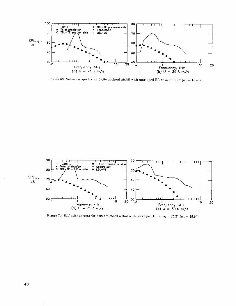
SPL1/_ ,
dB
1O0
90
80
I I I I Ill i I I I I I I 1 IIU
- Data : TBL-TE press re side* Total prediction Separation
--0 TBL-TE _n side O LBL-VS
/ \
70 -- i, _ _ __r
11
60.2 I ,, ,,,,I _ , ?_,,,,I I1 10 20
Frequency, kHz
(o) U = 71.3 m/s
8O
70
60
50
4O.2
' ' '''"1 ' ' ' '''"1
¢r
I I llllll I_ li I I I I II I
1 10 20Frequency, kHz
(b) U = 39.6 m/s
Figure 69. Self-noise spectra for 5.08-cm-chord airfoil with untripped BL at at = 19.8 ° (c_, = 15.4°).
SPL,/3 ,
dB70 -_
60 -
50.2
I I I I I I I I I I I I I I II I- Dote .,_ o TBL-TE pressure side
•Ir Totolzl_re_l_ct!on . A Seporotion
, J , ,,,,I , _, ,,_,I1 10 20
Frequency, kHz
(a) U = 71.3 m/s
70 I I I I III I I I , I I ,III! I
60t_
50 -- _ _r_'__
4-0 --
i i
30' J , , lJlll I J , , ,Jill.2 1 10
Frequency, kHz
(b) U = 39.6 m/s
Figure 70. Self-noise spectra for 5.08-cm-chord airfoil with untripped BL at at = 25.2 ° (a, = 19.6°).
I
20
48

SPL1/_ ,dB
100
90
I I I I I I I I I I I I I I I _'i ji, i{- Data l a TBL-TE pressTotal prediction ,_ Separation L _1
70 -
60.2 1 10 20
Frequency, kHz(o) U = 71.3 m/s
gO ' ' ' ''"I _ ' ' ' ''"I
8,0 _ __ --_i
70 -- @ --0
60 --
50 , , , lililJ, , i , ,,,,I L_
.2 T 10 20Frequency, kHz
(c) u = 39.6 m/s
1O0
90 --
80 --
70 --
6O.2
8O
70--
60--
50--
40.2
I I I 1 II I I I I IIIII I 1
Q @
I I I I I1[
1 10 20_'reque ncy, kHz
(b) U = 55.5 m/s
' ' ''''1 ' ' ' '''"1
° e _ --"
1 10 20Frequency, kHz
(d) U = 31.7 m/s
Figure 71. Self-noise spectra for 2.54-cm-chord airfoil with untripped BL at (_t = 0° (_, = 0°) •
SPL1/3 ,dB
I Dotlol i i i i i I I 0 ITBL_TEI i ipressureli i I . I I |80 - sldell 70 I I I I i I l i i i i i i i 1/* Total prediction & Separation /
70 0 TBL-TE suction side o LBL-VS --I 60 __._._ _[_ -'-_/
e • _ =aT__50 . . _ 4o . o _I
o I I@ []
402 , , ,,,,,I ,o, , ,,,,,18 _ 30 , , ,,,,,I , , , ,,,?,I II 10 20 .2 I 10 20
70
60--
50--
40--
30.2
Frequency, kHz(a) U = 71.3 m/s
' '''"1 ' ' ' '''"1
@ ,", o 8
I I I I Ill I I I I I I IqllT
1 10 20Frequency, kHz
(c) U = 39.6 m/s
60
50 --
40 --
30 --
20.2
I I
I I
Frequency, kHz(b) U = 55.5 m/_
'''"1 ' ' ' '''"1
[] --
• o
,J,,,l , , , ?,,,,I o1 10 20
Frequency, kHz(d) U = 31.7 m/s
Figure 72. Self-noise spectra for 2.54-cm-chord airfoil with untripped BL at c_t = 5.4 ° ((_, = 4.8°).
49
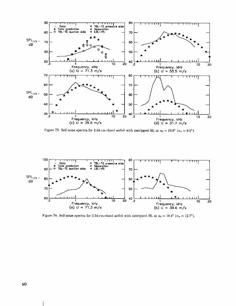
SPLI/a ,
dB
SPL1/_ .
dB
9O
8O
70--
60--
50._
70
6O
50
4O
30.2
I I I I III iData
• " Total predlct[on_ 0 TBL-TE suction side
I I I I I I I I
o TBL-TE pressure side& Separationo LBL-VS
trt_t
_ VO it
_ 9, _ , P_,_I , , , I I ll=l
1 10
Frequency, kHz
(o) U = 71.3 m/s
' ' '''"1 ' ' ' '''"1
J I t llll I I I I I Itll It
1 10
Frequency, kHz
(C) U = 39.6 m/s
2O
2O
80
70--
60--
50--
40.2
80
70 --
60 --
50--
40.2
I I i Inn I U U n _U nl_ I
_ i i I I t111 I I I I I iii I
1 10
Frequency, kHz
(b) U = 55.5 m/s
'_"1
, .",,,,,I , , ,,,,,,,I1 10
Frequency, kHz
(d) U = 31.7 m/_
Figure 73. Self-noise spectra for 2.54-cm-chord airfoil with untripped BL at at = 10.8 ° (a, = 9.5°).
2O
I
2O
SPLII3 ,
dB
1O0
go
80
7O
60.2
' ' ' ''"1 ' ' ' ' ''"1- Data o TBL-TE pressure side
_r Total predictTon z_ Separation_ o TBL-TE suction side <> LBL-VS
, , , ,,,,I , , = , n_,,,l
1 10 20
Frequency, kHz
(o) U = 71.3 m/s
80
70--
60
50 --
40.2
I I U I I II I I I i I I l II I
n , , ,,,,n n i n n anJlI 10
Frequency, kHz
(b) U = 39.6 m/s
Figure 74. Self-noise spectra for 2.54-cm-chord airfoil with untripped BL at at = 14.4 ° (c_, = 12.7°).
20
5O

5. Spectral Scaling
In this section, the scaling laws are developedfor the five self-noise mechanisms. The spectra of
figures 11 to 74 form the basis of the scaling forthree of the mechanisms: turbulent-boundary-layer-
trailing-edge (TBL-TE) noise and separation noise
were scaled from the tripped boundary-layer cases,
and laminar-boundary-layer-vortex-shedding (LBL-
VS) noise was scaled from the untripped cases. Forthe tip vortex formation noise mechanism, both the
data and the scaling approach are obtained from ref-
erence 18. Finally, for TE-bluntness vortex-shedding
noise, spectral data from the study of reference 2, as
well as previously unpublished data from that study,
form the basis of scaling analysis.
5.1. Turbulent-Boundary-Layer-Trailing-EdgeNoise and Separated Flow Noise
What has become traditional TE noise scaling is
based on the analysis of Ffowcs Williams and Hall
(ref. 5). For the problem of turbulence convecting at
low subsonic velocity Uc above a large plate and past
the trailing edge into the wake, the primary result is
(P2) C(t'0 -_0 _ D (17)
where (p2 / is the mean-square sound pressure at the
observer located a distance r from the edge. Themedium density is P0, vP2 is the mean-square tur-
bulence velocity, cO is the speed of sound, L is thespanwise extent wetted by the flow, and/: is a charac-
teristic turbulence correlation scale. The directivity
factor D equals 1 for observers normal to the surface
from the TE. The usual assumptions for boundary-
layer flow are that v I cx Uc <x U and £ c( 6 or 5",
where 5 and 5* are, respectively, the boundary-layer
thickness and displacement thickness. Fink (ref. 25),
when normalizing airframe noise data where TBL-TE noise was believed to be dominant, assumed
a universal spectrum shape F(St) for the noise,where St is the Strouhal number fS/U. The shape
F(St) depended only on the ratio of St to its peak
value Stpeak. This gave the following normalizationform for the 1/3-octave sound pressure level spectralpresentation:
SPLu3 - 10 log 1-_
with SPL1/3 = OASPL + F(St) and where K is anempirical constant which was determined when the
velocity U is given in units of knots.
As mentioned in section 1, some of the airfoil self-
noise spectral data of the present report were pre-sented, in uncorrected form, in reference 6, and nor-
malized in the manner of equation (18) using mea-sured values of/i. It was found that, contrary to what
was previously assumed (e.g., refs. 25 and 3), the nor-
malized levels, spectral shape, and Strouhal number
were not independent of airfoil size, airfoil angle of
attack, and free-stream velocity. However, the lim-
ited scope of the paper, as well as the uncertainty
caused by the aforementioned extraneous noise con-
tamination of the uncorrected spectra, prevented a
clear definition of the functional dependences. The
corrected spectra of the present report are used to de-
termine the parametric dependences and to accountfor these in the spectral scaling.
5.1. I. Scaled Data
Zero angle of attack. In figure 75, 1/3-octave
spectra for four airfoil sizes, each at four tunnel
speeds, are scaled. The spectra are obtained from
figures 11, 20, 26, and 32. The angle of attack is zeroand the boundary layers are tripped. The form ofthe normalization is
Scaled SPL1/3 = SPLu3 - 10 log (M 5 5_Lr-_) (19)
where Mach number replaces the velocity in knots, 6_replaces 5, and re replaces r. The retarded observer
distance re equals here the measured value, 122 cm
(see appendix B). For the right side of equation (19)to be accurately expressible by the form F(St)+ K of
equation (18), the scaled spectra of figure 75 shouldbe identical to one another for all cases. However,
the peak Strouhal number, spectral shape, and scaled
level vary significantly.
For each spectrum in figure 75, a symbol indi-cates the approximate spectral peak location. The
peak locations were based on gross spectral shapes
and trends rather than specific peak maximums. The
peak Strouhal number, Stpeak ---- (f S* /U)peak, andscaled levels corresponding to these peak locations
are shown in figures 76 and 77, respectively, as a
function of Reynolds number Rc. These data are
also presented in table 1 (at the back of this re-
port). Included in the figures are the other cases for
tripped BL airfoils of different chord lengths. Alsoincluded are data at nonzero angle of attack for sub-
sequent discussion. The displacement thicknesses for
the suction side, 5_, are used for these normaliza-
tions. In figure 76, Stpeak for zero angle of attack(solid symbols) shows no clear Rc-dependence, but a
Mach number dependence is apparent. The horizon-
tal lines through the data correspond to the function
51
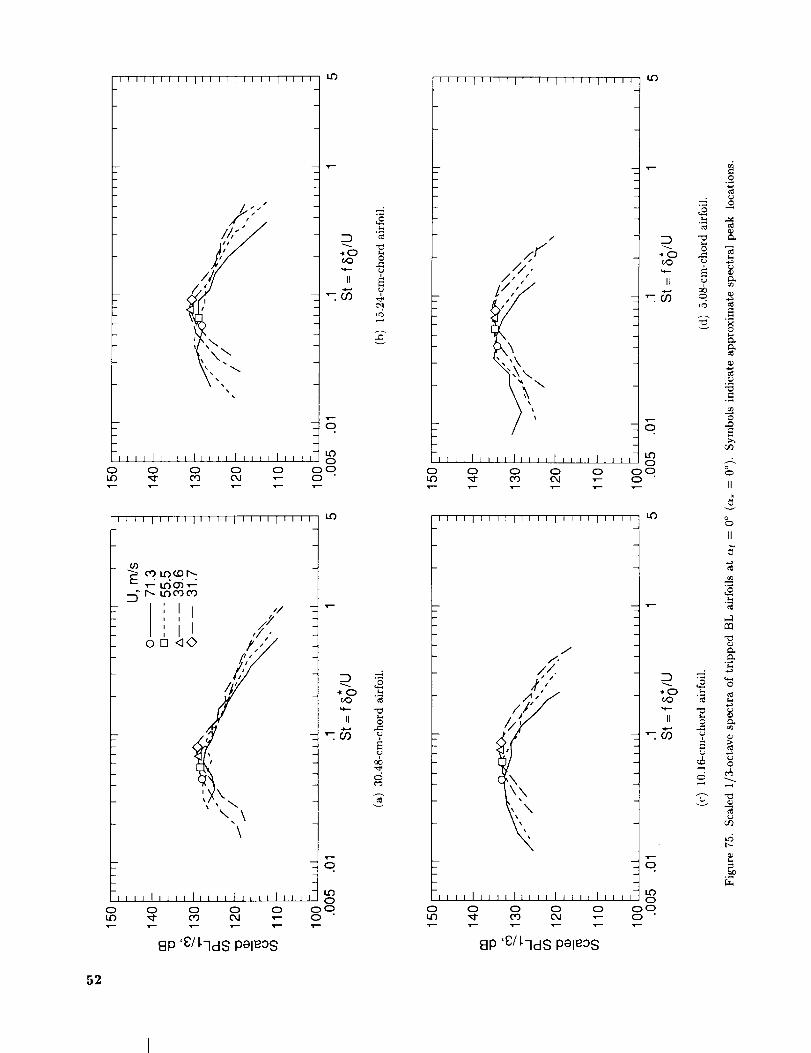
G2
IFIllllllltttllttttltttt
Y
\,\b\,,;-
JlnllJJllllll_lnJJlllll
0 0 0 0 0LO _ CO 04 _--
-_000
II
0
L_
C_C_
It lit il Ill It I uJ It lit II
I_ LZ")C'_0"3
!!l ":It ,/{
on qO /, ,_"/'./
:x,',\\ \
\
_'0sO
II
'_.00
0
L_It IIla t _n I_n a n I _l al laJ It 0
0 0 0 0 0 O0L_ _1" CO O,J T- 0
8P '8/l-ld S peleOS
,_.;
0
?
n
¢',1
0
O0
CO
InlJlnnnFluunFItrnnlJn
f
.kO
II
_C./3
0
oo o o o o oo
_ _ _ _ 0
tt ut I_l 17 I][ [n lit UllJU tn
/
i..¢")
._o
II-o..,-
"-:. C/)
oo o o o o ooL._ '_- co o,.I _'- o
8P '_/I'-IclS pel_0S
.o
._ o
L_
o
£
e.,
il
d
II
m
m
e_
2 _° _
,...I
d &
I'.-

g
oo
13_
] i _ I w , , J ] z i I i i i i ] I f i I i i i J ]
o_t' deg
,, • o+ 5.4
10.8
"&z& + + 14.4
.t"" O O,00 .,k 9 + 25.2 i
[] [] .-. [] _... A_ 0 9 U U,m/sL-J U -- _,.)A U .A A _I I _ U •
- -- OV _" _ / .093 31.7 _
-z-_--_ " - .116 39.6
Z-Z - _ • .. -. - - @ _.163 55.5St 1 nohA'.6 1 1 1 212 240464606 6 " \ .209 71.3....... 2 4 12 12 12 12
.01' ! I [ I I I | I I I I I _ i I i 1[ J J L _ _ _ i J
10 4 10 5 10 6 10 7
Reynolds number, R c
Figure 76. Peak Strouhal number for TBL TE noise versus Reynolds number. Numbers aligned with data are chord sizes in
inches (for brevity of notation).
150
m 140"O
_113_
co 130"O
a. 120
, , , , , I ''I ' ' ' ' ' ' ''1 ' ' '
oct' deg
5.4
'C'_'_ K 1 10 z_4 A_> 10"814.4.- ._, z,,,2 : .,,_ <>-- ^. ,.1 1 2 4 9 19.8[] _57_,1_4Lj4_7,_, g_ _ + 25.2
6_612612 12 12+ 9
I I l I I
110 I , , , L nnnl I I , _ i innl I I I , _ ''_
10 4 10 5 10 6 10 7
Reynolds number, R c
Figure 77. Peak scaled level for TBL TE noise versus Reynolds number. Numbers aligned with data are chord sizes in inches.
53
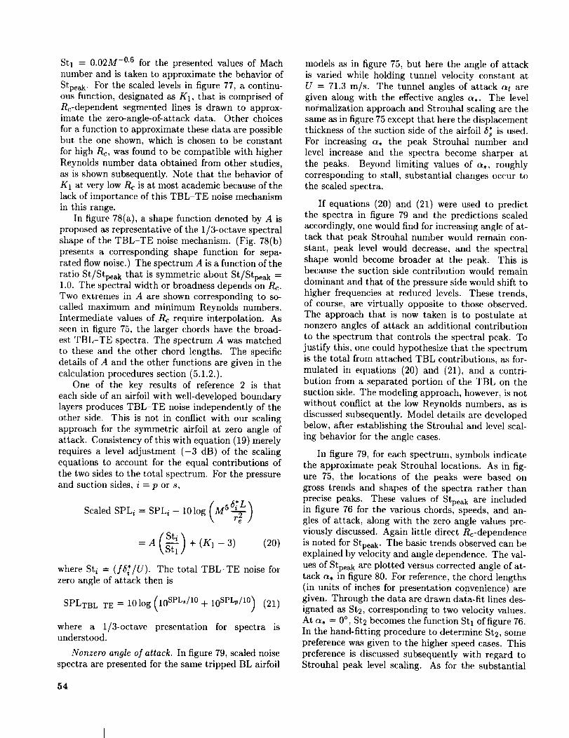
St1 = 0.02M -°'6 for the presented values of Mach
number and is taken to approximate the behavior of
Stpeak. For the scaled levels in figure 77, a continu-ous function, designated as K1, that is comprised of
Rc-dependent segmented lines is drawn to approx-
imate the zero-angle-of-attack data. Other choices
for a function to approximate these data are possiblebut the one shown, which is chosen to be constant
for high Rc, was found to be compatible with higher
Reynolds number data obtained from other studies,as is shown subsequently. Note that the behavior of
K1 at very low Rc is at most academic because of the
lack of importance of this TBL-TE noise mechanism
in this range.
In figure 78(a), a shape function denoted by A is
proposed as representative of the 1/3-octave spectral
shape of the TBL TE noise mechanism. (Fig. 78(b)
presents a corresponding shape function for sepa-
rated flow noise.) The spectrum A is a function of the
ratio St/Stpeak that is symmetric about St/Stpeak --1.0. The spectral width or broadness depends on Rc.
Two extremes in A are shown corresponding to so-called maximum and minimum Reynolds numbers.
Intermediate values of Rc require interpolation. As
seen in figure 75, the larger chords have the broad-
est TBL-TE spectra. The spectrum A was matched
to these and the other chord lengths. The specific
details of A and the other functions are given in the
calculation procedures section (5.1.2.).
One of the key results of reference 2 is that
each side of an airfoil with well-developed boundary
layers produces TBL-TE noise independently of the
other side. This is not in conflict with our scalingapproach for the symmetric airfoil at zero angle of
attack. Consistency of this with equation (19) merely
requires a level adjustment (-3 dB) of the scaling
equations to account for the equal contributions of
the two sides to the total spectrum. For the pressure
and suction sides, i = p or s,
Scaled SPLi = SPLi - 10log (M 56_L_
= A \Stl + (K1 - 3) (20)
where Sti = (f6_/U). The total TBL-TE noise forzero angle of attack then is
TE ----10log (10 SPL_/10 + 10 SPLp/10) (21)SPLTBL
where a 1/3-octave presentation for spectra isunderstood.
Nonzero angle of attack. In figure 79, scaled noise
spectra are presented for the same tripped BL airfoil
54
models as in figure 75, but here the angle of attack
is varied while holding tunnel velocity constant atU = 71.3 m/s. The tunnel angles of attack cq are
given along with the effective angles a,. The level
normalization approach and Strouhal scaling are the
same as in figure 75 except that here the displacement
thickness of the suction side of the airfoil 5" is used.
For increasing c_, the peak Strouhal number and
level increase and the spectra become sharper at
the peaks. Beyond limiting values of a,, roughly
corresponding to stall, substantial changes occur tothe scaled spectra.
If equations (20) and (21) were used to predictthe spectra in figure 79 and the predictions scaled
accordingly, one would find for increasing angle of at-
tack that peak Strouhal number would remain con-
stant, peak level would decrease, and the spectral
shape would become broader at the peak. This isbecause the suction side contribution would remain
dominant and that of the pressure side would shift to
higher frequencies at reduced levels. These trends,
of course, are virtually opposite to those observed.
The approach that is now taken is to postulate atnonzero angles of attack an additional contribution
to the spectrum that controls the spectral peak. To
justify this, one could hypothesize that the spectrum
is the total from attached TBL contributions, as for-
mulated in equations (20) and (21), and a contri-
bution from a separated portion of the TBL on the
suction side. The modeling approach, however, is not
without conflict at the low Reynolds numbers, as is
discussed subsequently. Model details are developedbelow, after establishing the Strouhal and level scal-
ing behavior for the angle cases.
In figure 79, for each spectrum, symbols indicate
the approximate peak Strouhal locations. As in fig-ure 75, the locations of the peaks were based on
gross trends and shapes of the spectra rather than
precise peaks. These values of Stpeak are includedin figure 76 for the various chords, speeds, and an-
gles of attack, along with the zero angle values pre-
vionsly discussed. Again little direct Rc-dependence
is noted for Stpeak. The basic trends observed can beexplained by velocity and angle dependence. The val-
ues of Stpeak are plotted versus corrected angle of at-
tack a. in figure 80. For reference, the chord lengths
(in units of inches for presentation convenience) aregiven. Through the data are drawn data-fit lines des-
ignated as St2, corresponding to two velocity values.
At a. --- 0 °, St 2 becomes the function Stl of figure 76.
In the hand-fitting procedure to determine St2, some
preference was given to the higher speed cases. This
preference is discussed subsequently with regard to
Strouhal peak level scaling. As for the substantial
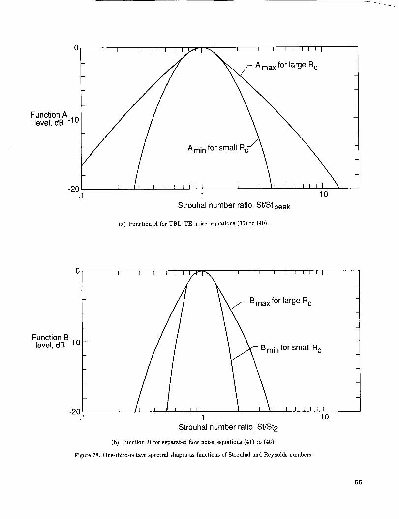
0
Function Alevel, dB -10
-20.1
I I I I
I I I I I I I
A max for large Rc
A min for small R
Illl I1
Strouhal number ratio, St/St peak
(a) Function A for TBL-TE noise, equations (35) to (40).
10
m
i
0
-2O.1
Function Blevel, dB -10
I I I I I I i I I I
B max for large Rc
B min for small Rc
1
Strouhal number ratio, St/St 2
(b) Function B for separated flow noise, equations (41) to (46).
Figure 78. One-third-octave spectral shapes as functions of Strouhal and Reynolds numbers.
10
55

56
II
,-:._
0 0 0 0 0 O0_ _ _ _ 0
ii li I_l JI lii If I il il Ill IFo o
b _'°°,:c6_
_" S u-i d 4
I!!l: II /;
on<]O /,p"
./,//2"
/
\
ti
_.r/?
0
0 0 0 0 0 O01.0 _ CO OJ T- 0 "
8P '_/l-ldS Pel_oS
o..s:
o
ob
¢o
o o o o oo OJ "_"CXI "_"_.0
0 0 0 0 0 I I [ I I I I [ I I I I"-' o _- 00',_- _00,I
o_c_,_c_•,-',-',-OJ /
, i i /i I , ,i i ' i i / ,
', II I I /" /""o []<]0-4 _, ....'"
,_ .
/ {"'..<'"
'V,/" \ "
'\:
kO
=)
._(,0_0
II
"z. r./)
0
0 0 0 0 0 O0'_- CO 04 _-- 0 "
_ _ n nol$%U_J 6u u u u I I I I n I ; u ; _
- * o O')l"--_O, lqC)
__ om_05ai_ , .."i .*
--o _-_o_-_o_ /:.o_d_o_
•-- _.,-0,1 ,('"
'l ',: /:'',,I, i ..'',111:/ /
on._Oz_, i /
.._..::J
\k
It
0
0o o o o o oo
_ O_ OJ .,- 0
8P '8/LldS peleoS
o
¢.-,-,.f
ooo
LO
©e-?
.S
o
II
"_,

data scatter of figure 80, some comments are war-ranted. It was found that if one used the actual mea-
sured values of 6_ (where available) in the Strouhal
scaling, one would have a similar degree of scatter
to that shown in figure 80, where scaled values of
6_ (eq. (12)) were used. Also if untripped BL air-
foil results were plotted, for those limited number of
cases where the LBL-VS shedding source is not ap-
parent in the spectra, the scatter and trend would be
about the same as those shown in figure 80. Otherdeviations of the data from the St2 lines occur at
mid to high angles of attack, where the low-frequency
parts of the spectra were limited by the experimental
high-pass filtering and thus values of Stpeak were in-accurately large. The behavior of St2 seen in figure 80at the higher angles of attack (where the horizontal
lines are placed lower than the data) was chosen to
approximately correct this bias.
The scaled levels corresponding to spectral peaks
chosen in figure 79 are shown in figure 77 with
the other cases. The previously indicated conflict
within the data base for the proposed modeling ap-
proach, which hypothesizes contributions from two
attached TBL's and an angle-dependent separation-
related portion, is seen in figure 77. Peak levels for
the two smallest chord lengths, except at the highestspeeds, significantly decrease as the angle of attack
increases from zero. This is incompatible with the
modeling approach. A choice is made to ignore the
conflicting low Reynolds number data in the model
development. While admitting that the inclusion of
the low Reynolds number behavior would conceptu-
ally be desirable for completeness of the modeling,
the exclusion is believed justifiable because of the
greater interest in higher Reynolds number condi-tions. The TBL-TE noise mechanism is not con-
sidered important for low Reynolds numbers. Evenif this were not the case, it is not certain that the
present test flow conditions with heavy leading-edge
tripping for airfoils at nonzero angles of attack prop-
erly represent the mechanism, especially for higher
angles where relaminarization of the pressure-sideboundary layer is possible. Regardless, the results
of the scaling are compared subsequently with the
spectra of all the data to allow a direct assessment of
the effect of modeling choices.
The scaled levels of figure 77 for chord lengths
of 10.16, 15.24, 22.86, and 30.48 cm are plotted
in figure 81 versus a,. If the portion of these
levels that cannot be accounted for by the modelingof equations (20) and (21) can be extracted, this
portion would be designated as the separated flow
noise contribution. Calculations were performed by
taking into account that the Strouhal dependence
of A in equation (20) would follow St1 of figure 76
rather than St2 of figure 80, which applies to that
portion extracted. The extracted levels are given
in figure 82. These extracted levels are normalized
by subtracting the zero-angle-of-attack function of
figure 77 (K1) for the particular chord lengths and
speeds. Although substantial scatter is present, a
basic trend of increasing importance for increasing
angle and speed is seen. Drawn through the data is
a function designated as K 2 - KI which represents
a partially observed, partially postulated dependence
on velocity and angle of attack. The assigned spectralshape for this additive source is function B, which
is given in figure 78(b) and is defined in a manner
similar to function A of figure 78(a) to have a widthwhich is dependent on chord Reynolds number.
The resulting scaling model for the angle-dependent noise SPLa is
/ __*L\Scaled SPLa = SPLa - 10 log/m5 "-/
t, )
(St_'_= B t, St_2/ + K2 (22)
where this represents the separated-boundary-layernoise contribution to the total noise. The total TBL-
TE and separation noise is then
SPLTo T = lOlog (10 sPL"/IO + 10 SPL'/I°
+ IoSPLp/10) (23)
During development of the scaling procedures,
equations (20), (22), and (23) were compared withspectra for all tripped BL airfoils and with spectra
for the untripped BL airfoils for which TBL-TE noise
appeared to significantly contribute. Analyses of
comparisons resulted in optimization of curves A and
B, as well as development of the specific calculation
procedures. The analysis found that better results
are obtained when the Strouhal dependency of the
suction-side spectrum SPLs is (St 1 + St2)/2 ratherthan Stl. It was found that for better SPL agree-
ment, one should make an adjustment in pressure-
side level SPLp (defined as AK1 in the following sec-tion) as a function of angle of attack and Reynolds
number based on the displacement thickness 6_. Thisadjustment diminishes the pressure-side contribution
for increasing angle and decreasing velocity. Also it
was found that the drastic spectral shape changesthat occur at sufficiently high angles of attack, near
stall, are roughly simulated by a calculation proce-
dure change. At the value of a, corresponding to
the peak of the appropriate /(2 curve, the spectral
57
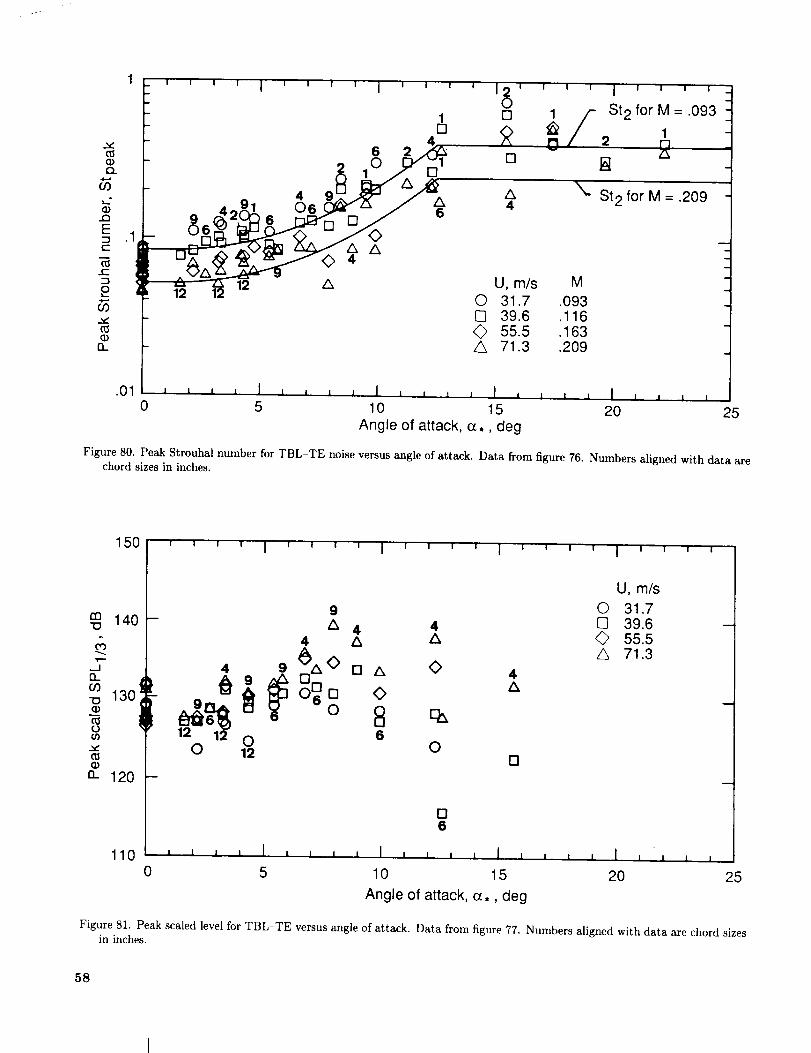
O..
03
E
E
t-:}
£03
13_
. _ i i I I i i 'i I I , I i
5i 4
6 2 '
12 12
' 12'0[]
[]
4
U, m/s M0 31.7 .093[] 39.6 .116<_ 55.5 .163,_ 71.3 .209
1 /- St2f°rM= .093
/ 1 -
_- St 2 for M = .209
.01 , , , , I , , , , 1 , i i , 1 , j l , I _ , , ,0 5 10 15 20 25
Angle of attack, (z,, deg
Figure 80. Peak Strouhal number for TBL-TE noise versus angle of attack. Data from figure 76. Numbers aligned with data are
chord sizes in inches.
150
140
130'
n 120
- 44 4 A
oO 10 O
4A
13
136
U, m/s
© 31.739.6
© 55.5Z_ 71.3
110 L , l _ , I , , , _ I _ , , _ I , , _ , I , j _ ,0 5 10 15 20 25
Angle of attack, o_., deg
Figure 81. Peak scaled level for TBL-TE versus angle of attack. Data from figure 77. Numbers aligned with data are chord sizes
in inches.
58

contributionsSPLsand SPLpin equation(23)areeliminatedandthe B curve of equation (22) is re-placed by an A curve corresponding to a value of Rcwhich is three times the actual value.
The calculation procedures are specified in thenext section followed by comparison with the spectraldata base.
m20
,,i
2O
10
' ' ' ' I ' ' ' ' I '
ZX
' ' ' I ' ' ' ' I ' ' ' '
U, m/s M
O 31.7 .093
[] 39.6 .116c 6A 46 4 Ar: .. 9 A vIL_A__ - A \/"
o-
..16 13 . 9
_20| , , , I , , , , I , , , , t , , io 5 10 15
Angle of attack, a., deg
55.5 .163
71.3 .209
K2 -K 1
I I I I I t
20 25
Figure 82. Angle-dependent scaled noise levels as referenced to zero angle of attack, TBL TE noise model. Numbers aligned
with data are chord sizes in inches.
5.1.2. Calculation Procedures
The total TBL-TE and separation noise spectrum in a 1/3-octave presentation is predicted by
SPLTo T = 10 log (10 SPLc'/10 4- 10 SPLs/10 4- 10 SPLp/10) (24)
where
(5_MSL-Dh_ (Stp'_SPLp = 10 log + A\ re / k_]
SPL, = 10log (6*_Dh5 4-A (St,_\ r e / \Stl]
+ (K] - 3) + AK1 (25)
4- (K1 - 3) (26)
and
SPLe= lOlog(_f;iSL-Dhl 4- B(Sts_\ re ] \St2] + K2
for angles of attack up to (e,)0, an angle to be defined later in this section. At angles above (a,)0,
(27)
SPLp = -oo (28)
SPLs = -oo (29)
59

and
SPLa= lO log ( 5* M_L-Dt _ +A,(sts5\St2] + K2 (30)
where A' is the curve A but for a value of Rc which is three times the actual value. The directivity functions
D h and De are given in appendix B by equations (B1) and (B2), respectively.
The Strouhal definitions are (see figs. 76 and 80)
Stp- f6pu Sts -- _f6* (31)
St1 = 0.02M -°6 (32)
S--tt - St1 + St2 (33)2
and
St 2 = St I x {
1 (a, < 1.33 °)
100'0054(a*-1"33)2 (1.33 ° < a, _< 12.5 °)
4.72 (12.5 ° < a,)
(34)
For the spectral shape function definitions, we first consider the function A of figure 78(a). As discussed,
the function A for a particular Reynolds number Rc is obtained from an interpolation of the curves A,nax and
Ami n corresponding to chosen values, (Re)max and (Rc)min. The two curves are defined as
Amin(a) = {
,/67.552 - 886.788a 2 - 8.219
-32.665a + 3.981
-142.795a 3 + 103.656a 2 - 57.757a + 6.006
(a < 0.204)
(0.204 < a < 0.244)
(0.244 < a)
(35)
and
Amax(a) ={
x/67.552 - 886.788a 2 - 8.219
-15.901a + 1.098
-4.669a 3 + 3.491a 2 - 16.699a + 1.149
(a < 0.13)
(0.13 < a < 0.321)
(0.321 < a)
(36)
where a is the absolute value of the logarithm of the ratio of Strouhal number, St = Stp or Sts, to the peak
Strouhal number, Stpeak ----Stl, Stl, or St2:
a = I log(St/Stpeak)t (37)
The absolute value is used because the spectral shape is modeled to be symmetric about a = 0.
The interpolative procedure includes defining a value, a0(Rc), at which the spectrum has a value of -20 dB.
This -20 dB corresponds to a horizontal axis intercept in figure 78(a) for an interpolated curve. The function
6O

ao(Rc) is given by
0.57
ao(Rc) = (-9.57 x 10⁻¹³)(Rc - 8.57 x 10⁵) 2 + 1.13
1.13
(Rc < 9.52 x 10⁴ )
(9.52 x 10⁴ _< Rc <_ 8.57 x 10⁵ )
(8.57 x l05 < Rc)
(38)
An interpolation factor AR(aO) is determined from
-20 - Amin(aO)
AR(aO) = Amax(ao) - Amin(ao)(39)
where Amin(a0) and Amax(a0) are the Amax and Ami n spectra evaluated at a 0. The spectrum shape A can now
be evaluated for any frequency by computing the Strouhal number St and the corresponding a and using the
interpolation factor. The result for use in equations (25), (26), and (30) is
A(a) = Amin(a ) + AR(ao)[Amax(a) - Amin(a)] (4o)
The function B in equation (27) and shown plotted in figure 78(b) is calculated in a manner similar to
function A above. The two curves Bmax and Brain, through which B is obtained from interpolation, are
V'16.888 - 886.788b 2 - 4.109 (b < 0.13)
Brain(b) = -83.607b + 8.138 (0.13 < b < 0.145)
-817.810b 3 + 355.210b 2 - 135.024b + 10.619 (0.145 < b)
(41)
and
where
Bmax(b) = {
x/16.888 - 886.788b 2 - 4.109
-31.330b + 1.854
-80.541b 3 + 44.174b 2 - 39.381b + 2.344
(b < 0.10)
(0.10 < b < 0.187)
(0.187 < b)
(42)
b = I log(Sts/St2)l (43)
The spectral shape B for intermediate values of Rc have horizontal axis intercepts at -20 dB in figure 78(b)
for values of b of
0.30
bo(Rc) = (-4.48 x 10⁻¹³)(Rc - 8.57 x 10⁵) 2 + 0.56
0.56
(Rc < 9.52 x 10⁴)
(9.52 x 10⁴ < Rc <_ 8.57 x 10⁵)
(8.57 x 10⁵ < Rc)
(44)
The interpolation factor BR(bo) is defined as
-20 - Bmin(b0)
BR(bo) = Bmax(b0) - Bmin(b0)(45)
and thus the result for use in equation (27) is
B(b) = Brain(b) + BR(bo)[Bmax(b) - Brain(b)] (46)
61

TheamplitudefunctionK1 in equations (25) and (26) is plotted in figure 77 and is given by
-4.31 log(Rc) + 156.3
K1 = -9.01og(Rc) + 181.6
128.5
(Rc < 2.47 × 10⁵)
(2.47× 10⁵_<Rc<8.0× 10⁵ )
(8.0 x 10⁵ < Re)
(47)
The level adjustment previously mentioned for the pressure-side contribution for nonzero angles of attack
appears as AK1 in equation (25). This is given by
(
AK1 _-- _ c_,
[ 0
[, (R_; < 5000)
(5000 < R_;)
(48)
where RS_ is the Reynolds number based on pressure-side displacement thickness.
The amplitude function/{2 of equations (27) and (30) is plotted for some values of M in figure 82 and is
given as
K2 = K1 + {
-1000
V//32_ (/3/_)2(a, _ .y0)2+/3o
-12
(a, < "_0 - "_)
('_0 -'_ -< a, <_ "Y0 + "/)
(_0 + "Y< _,)
(49)
where
-), = 27.094M + 3.31
/3 = 72.65M + 10.74
"_0 = 23.43M +4.651 /
ffl0 = -34.19M- 13.82(50)
The angle definitions above are in units of degrees and are taken as positive in sign. The K2 definition
above is valid for all values of a,, even when the calculation of the total noise in equation (24) switches from
the use of equations (25), (26), and (27) for assumed attached TBL flow to equations (28), (29), and (30) for a
supposedly stalled flow condition. The angle where the switch occurs, specified previously as (a,)0, is taken to
be equal to the peak of the K2 function defined by "Y0 in equation (50) or whenever a, exceeds 12.5 °, whicheveris first.
5.1.3. Comparison With Data
The scaling predictions of TBL-TE and separa-
tion noise are compared with the noise data in fig-ures 11 to 43 for the tripped BL airfoils. The cal-
culations used the appropriate values of 6" from sec-
tion 3 and the directivity functions from appendix B(where re = 1.22 m, Oe = 90 °, and (I)e = 90°). The
total self-noise is given as well as the individual noise
components of TBL TE noise from the suction and
pressure sides and separation noise. The predictions
follow the shapes and levels of the data, especially
for the larger airfoils and the lower angles of attack
where the scaling accuracy was most emphasized.
Predictions of TBL TE and separation noise are also
shown for the untripped BL airfoils in figures 44
to 74. For the many untripped cases where these
sources are predicted to be dominant, the agreementis generally good. Even where the LBL VS noise
dominates, the TBL TE and separation contribu-
tions help with the overall spectral agreement.
5.2. Laminar-Boundary-Layer-Vortex-
Shedding Noise
As previously described in section 1, laminar-
boundary-layer instabilities couple with acousticfeedback to produce quasi-tonal noise. In contrast to
TBL-TE noise, there are no LBL VS noise scalingmethods established in the literature because of the
erratic behavior of the multiple tones in the narrow-
band spectra and the general complexity of the
62

mechanism. Two key results from the literature
which provide initial scaling guidance are (1) that
the gross trend of the frequency dependence was
found to scale on a Strouhal basis, with the relevant
length scale being the laminar-boundary-layer thick-
ness at the airfoil trailing edge (ref. 16), and (2) thaton the basis of the limited data from the data base of
the present paper as reported in reference (6), overall
levels tended to coalesce to a unique function of Rcwhen normalized in the fashion of TBL-TE noise.
The scaling approach taken herein is similar tothat taken for TBL TE noise in the last section in
that a universal spectral shape and Strouhal depen-
dency is modeled in terms of boundary-layer param-
eters, Mach number, angle of attack, and Reynolds
number. The use of 1/3-octave spectra, rather than
narrow band, permits such an approach because the
broad spectral bands overlap the tonal frequency
spacing to give smoother and generally single-peaked
spectra.
5.2.1. Scaled Data
Scaled 1/3-octave sound pressure level spectra for
four airfoil sizes, each at four tunnel speeds, are
presented in figure 83 from figures 44, 53, 59, and 65.
The angle of attack for all is zero and the boundary
layers are untripped. The normalization employs
Scaled SPL1/3 = SPL1/3 - 10log (M 55pL'_rl ) (51)
for level scaling and
st'- lip (52)U
for Strouhal frequency scaling. For the symmetric
airfoils at zero angle of attack, 5p = 6s = 50.
The scaling approach differs from the TBL TE noise
scaling because of the use of 6p, the boundary-layer
thickness on the pressure side of the airfoil, rather
than 5", the boundary-layer displacement thickness
on the suction side. The use of 5p as the pertinent
length scale follows from reference 16 and was found
to give seemingly better results in initial scaling of
the present data base than 5_ and by far better than
c, 6s, or 6_ for angles of attack other than zero.
In figure 83(a) for the large 30.48-cm-chord air-
foil, the spectra appear to be of smooth broad hump
shapes. There is no apparent contribution to the
spectra from LBL-VS noise which is peaked in char-acter. The boundary layers are fully turbulent in
the vicinity of the trailing edge at all four tunnel
speeds (ref. 21), so no laminar vortex shedding is
established. The noise produced is assumed to beall TBL TE noise. In figure 83(b) for the 15.24-cm-
chord airfoil, the broad spectral shapes are changed
by the addition of a peak when the flow velocity isdiminished. The peak levels increase with decreasing
velocity. Although the boundary layer is turbulent at
the trailing edge at all velocities shown, laminar flowexists over larger portions of the airfoil at the lowervelocities. As mentioned for the LBL-VS noise mech-
anism, any spectral peaks containing a number oftonal contributions should scale with Strouhal num-
bers based on boundary-layer thickness. This is the
case in figure 83(b) with St r _ 0.27. For the shorter10.16-cm-chord airfoil, in figure 83(c), the LBL VS
noise peaks become even more dominant for decreas-
ing velocity. Note also the changing Strouhal depen-
dence, not noted in previous studies. The shorter
5.08-cm-chord airfoil, in figure 83(d), has even more
pronounced level and Strouhal dependence with ve-
locity variations.
Whereas figure 83 shows the dependence of LBL
VS noise on velocity for the various airfoil sizes at
zero angle of attack, figure 84 shows the effect of
angle of attack a, of the airfoils at a velocity of
71.3 m/s. The spectra for the 30.48-cm-chord airfoil,shown in figure 84(a), change from being dominated
by TBL TE noise, for c_, = 0 °, to being dominated
by LBL VS noise, for c_, = 4.0 ° . So even with a
large Reynolds number (Rc = 1.52 × 10⁶), LBL-VS
noise occurs. With increasing a,, the boundary layer
on the pressure side becomes more laminar over asufficiently large portion of the chord to result in in-
creased shedding and corresponding noise. For the15.24-cm-chord airfoil (Rc = 7.58 × 10⁵), shown in
figure 84(b), the LBL-VS noise increases with c_, un-til a certain value is reached where it diminishes. At
a, = 7.2 °, no apparent shedding noise is shown. At
o_, = 9.9 °, the noise changes appreciably to that forstalled flow as discussed in the last section. The use
of 5p as the characteristic length scale apparently re-sults in-a proper Strouhal scaling for the shedding
noise peaks; but, as expected, the spectra for a, =0 °, 7.2 °, and 9.9 °, which are dominated by TBL-
TE and separated flow noise, diverge in this nor-
malized format. A similar angle-dependent behavior
where spectra do not coalesce is seen for the10.16-cm-chord airfoil, in figure 84(c), where LBL
VS noise is apparent at c_, = 0° and 3.3 ° but not
at the higher angles. For the 5.08-cm-chord model,
figure 84(d) shows large-amplitude LBL VS noise ata, =0 ° and 4.2 ° .
63

lllifftJllillltrtltll
<]
//
/ .J
//I
.// ,-
&,,"
:J 11 Ill II Ill Jl I :j :j IIjj
C) 0 0 C) 0LC) _ CO 04 ---,r- .r-- _-- .r--- .r'-
IlillllirfilJtlllJill
E .--_ o'_,-
I'!' I!jr
oDqO
/4 S//
4";"# 14
/,/,'_//,V
X,,\\
tt IJllt tliltlllitllJltt
0 0 0 0 0_1" 03 OJ ,,--
8P 'E;/L-iclS Pale0 S
1 I..0
::30
II
0
E:)OC)C_ "
0uO
II
0
LOI 0O00 "
0
?c"q
o.J::::
0o
C:) (Z:) 0 CZ) 0O0 I_ _ _
iiilllll[lil i it il iii li I._
{' _._
.i' &.
'_. r..f)
k\, ",
\ \\,_,\ ,
0
LO0
O003 '
0£0
/
.....<_-.--m3 [ o
0
U")_ _1_ _ I_i _ljl_ 0
0 0 0 E:) O0
gp 'E;/Lqd S Pele0S
r../3;>
"-4 I:£
•.J:: o
ui0o
o
00
II
II
°-
,.2o
,.£ _.
o "_
' _ ¢,p
_2
64

o_D
0L_
,-t.-.
II
o
oOO,r-
I IIIII IIIIt IJlll II1,1 IIo
o _0_s
I'" II /S
/ /6
ff
li f "
I,\\\
/
I
I
i
I
I \
LO
0
- LOliiiliillliililll illll iI 0
0 0 0 0 O0_- _ (Xl _- 0 "
8P '_/l'-IdS Pele0S
::D
CL
,-i--.
tl
0
Y.,?,
0
Y
YoO
o
It II lit Illlllllllllllll
o o o o
l, ! 'I I
,' IIIo []<ION
[]
II I , I , , , , II , _"_ I i, , i I l, i 0
0 0 0 0 O0LO _" O_ O_ "
_O
II
I I I
4,
i I I I
o
u_I IOI I011011 I I I I I I l 11 I I I I0
o eO I_ (3_(_I
o o o
o '_- O0 _" O0
i,! 'I I
' IIII
o []<]ON
.-" 0
II
/ \ 1 _-o.
I I I i i i I i_ i I I I , i i I I , i i/ i'O0
0 0 0 0 O0I.i"l _ CO _ '
8P 'O/LGclS PeleoS
0
v
©
F;
..=
0
II
.£
_0 I.-,
b,O
E,
65

The LBL-VS noise portions of the spectra
(figs. 83 and 84) are rather invariant with respect
to spectral shape. Based on this observation, a func-
tion G1 (shown in fig. 85) was chosen as a shape to
represent the LBL-VS contribution to the self-noise
1/3-octave spectra for all cases. The level of G1 at
St I -- Stpeak has a value of -3.5 dB. The referencelevel of 0 dB is the integrated total of G1. To permit
an orderly study of the Reynolds number and angle
dependences of the spectral data, the shape G1 was
matched to the individual spectra to obtain reference
overall peak levels and Strouhal numbers. Emphasis
was placed on matching the global spectral shape ofG1 to the data rather than matching 1/3-octave band
peak or overall levels. Reference peak locations are
indicated by the symbols in figures 83 and 84.
!
In figure 86, the chosen values of Stpeak are plot-
ted versus the Reynolds number Rc for the 42 caseswhere LBL-VS noise is prominent. The values are
also given in table 2 (at the back of this report)
along with the effective angles of attack a, corre-
sponding to cq. For a, -- 0, Stpeak is approximatelyconstant at low Rc and increases with Rc in the mid-
range of Rc shown. The values of Stpeak are lower
for nonzero angles of attack. A function St_ is drawn
to approximate the data of zero angle of attack. A
constant value for St_ is chosen for high Rc, where
no zero-angle-of-attack data are present, because thevalue permits a simple angle dependence definition
J I
for Stpeak. In figure 87, Stpeak is normalized by St_
and plotted versus a,. For each of the six airfoils,the line described by 10 -0.040* approximates the an-
gle dependence.
5.2.2. Calculation Procedures
The reference peak scaled levels which correspondt
to Stpeak in figure 86 are plotted versus Rc in fig-ure 88. To show general trends more clearly, the
symbols are replaced by the value of (_,, rounded off
to the nearest whole degree (see table 2 for more ex-
act values). In this format it is seen that for eachc_, the scaled levels tend to increase, peak, and de-
crease as Rc increases. For the larger angles of at-
tack, the peak levels are lower and the corresponding
values of Rc are larger. Superimposed on the dataare curves of identical shape, called here "level shape
curves," which are positioned in a monotonically de-
creasing fashion to approximately correspond to the
data trends with angle variation. The angles indi-cated for each curve position should not necessarily
match the angle values listed for the data becausethe data values are rounded off in the figure, as men-
tioned. The intent is to use the curves, with their
functional relationship to (_, and Rc shown in fig-
ure 88, to represent the amplitude definition of LBL
VS noise. In the following calculation procedures sec-
tion, a function G2 specifies the curve shape, G3 is
the angle dependence for the level of the G2 curve,
and a reference (Rc)o value is defined as a functionof angle to specify the Reynolds number dependence.
The success of the functions in normalizing the data
is shown in figure 89 where peak scaled 1/3-octavelevel minus G3 is compared with the function G2.
In this format the individual angle numbers should
ideally match the G2 curve. Although the agreement
shown is certainly not complete, it is regarded here asacceptable. Note that much better curve fits to the
data would be possible if a requirement for mono-
tonic functional behavior had not been imposed on
G3 and (Rc)o.
The LBL VS noise spectrum in a 1/3-octave presentation is predicted by
SPLLBL VS = 10log r2 + G1 _Stpeak] + G2 (---R_c)0 + G3((_,)(53)
The Strouhal definitions are (see figs. 86 and 87)
(54)
0.18
St_ = 0.001756Rc 0"3931
0.28
(Rc_< 1.3× 10⁵ )
(1.3× 10⁵ <Rc_<4.0x 10⁵ )
(4.0 x 10⁵ < Rc)
(55)
66

Function G 1level, dB
-10
-20
-3O
! I I I | w I I i_ ! i s • . i • .
ce _____
i i I t
1
Strouhal number ratio, St'/Stpeak
Figure 85. One-third-octave spectral shape function G1 for LBL VS noise, equation (57).
I 5 i
I0
Srpeak .1
_ 4 9 4 St'l-4 _('5_ _ 12 /
6 9
o_t' deg
© 0[] 5.4<> 1o.8,_ 14.4
.01 i i ' , i J l,l l , , , , , ,ll
10 4 10 5 10 6
; I 1 I I I !
I I I I i i I i
10 7
Reynolds number, R c
Figure 86. Peak Strouhal number for LBL VS noise versus Reynolds number. Numbers aligned with data are chord sizes in
inches.
67

Stpeak
St "1
.5
(_ 2.54 cm chord
U_
m/s
0 31.7
13 39.6
<_ 55.5
71.3
15.24 cm chord
Stpeak
St "1
2
.5
5.08 cm chord I 22.86 cm chord
2
10.16 cm chord / 30.84 cm chord
F
|Stpeak
.50 5 0 5
oc,, deg o_,, deg
Figure 87. Peak Strouhal number for LBL VS noise versus angle of attack. Data from figure 86.
68

f13-O
(1)>a)
"ID
09
[3_
170
160
150
140
130
0
_ Level shape
"7./.0 4 10 5 10 6
Reynolds number, R c
, * L _ L ]
10 7
Figure 88. Peak scaled levels for LBL VS noise versus Reynolds number. Data symbols are values of a, rounded off to nearest
degree.
rn"(5
(3_o
¢-
E
>
"O
o¢o
[3_
0
-10
-2O
-3O
-4O
.1 1 10 100
Reynolds number ratio, R c/(R c)0
Figure 89. Normalization of LBL VS noise peak scaled levels by functions G2, equations (58) and (59), and G3, equation (60).
Data from figure 88. Data symbols are values of a. rounded off to nearest degree.
69

and
Stpeak = St_ × 10 -O'04a" (56)
m
The directivity function D h is given by equation (B1) in appendix B. The function G1 defines the spectral
shape, in terms of the ratio of Strouhal number to its peak, as (see fig. 85)
Gl(e) =
39.8 log(e) - 11.12
98.409 log(e) + 2.0
-5.076 + V/2.484 - 506.25[log(e)] 2
-98.409 log(e) + 2.0
-39.8 log(e) - 11.12
(e < 0.5974)
(0.5974 < e < 0.8545)
(0.8545 < e _< 1.17)
(1.17 < e _< 1.674)
(1.674 < e)
(57)
where e = Stl/Stpeak . The peak scaled level shape curve G2 depends on Reynolds number and angle and is
(see figs. 88 and 89)
a2(d) =
77.852log(d) + 15.328
65.18Slog(d) + 9.125
- 114.052[log(d)] 2
-65.188log(d) + 9.125
-77.852log(d) + 15.328
(d < 0.3237)
(0.3237 < d < 0.5689)
(0.5689 < d _ 1.7579)
(1.7579 < d < 3.0889)
(3.0889 < d)
(58)
where d = Rc/(Rc)o and the reference Reynolds number is
100.215a,+4.978(Rc)O = 100"120a*+5"263
The angle-dependent level for the shape curve is
G3(a,) = 171.04 - 3.03a,
(59)
(60)
70

5.2.3. Comparison With Data
The spectral predictions from the above equations
are compared with the untripped BL airfoil noise
data in figures 44 to 74. The great sensitivity of
this mechanism to angle and velocity change can
be clearly seen. In many respects the prediction
agreement in shape, level, and actual occurrence of
LBL-VS noise is good. Also as indicated in thelast section, the combined contributions of LBL VS,
TBL TE, and separation noise are important to the
total predictions for this untripped BL airfoil data.
5.3. Tip Vortex Formation Noise
The prediction method proposed in this section
for tip vortex formation noise is that developed by
Brooks and Marcolini (ref. 18). The study isolated
this high-frequency broadband self-noise by compar-
ing aerodynamic and acoustic test results of both
two-dimensional (2D) and three-dimensional (3D)
airfoil models shown in figures 2 and 3, respectively.
The premise of the tip noise determination methodwas that 3D models produce both tip noise and TBL-
TE noise, while the 2D models produce only the lat-
ter. The study produced a prediction method in gen-
eral agreement with the physical model of the mech-anism first proposed by George, Najjar, and Kim
(ref. 17). The noise is associated with the turbu-lence in the locally separated flow region at the tip
of a lifting blade, where the tip vortex is formed. Theflow field is illustrated in figure 90 for an airfoil blade
tip at an angle of attack O_TiP to the flow of velocityU. The flow over the blade tip consists of a vortex
of strength F with a thick viscous core whose span-wise extent at the TE is g. The recirculating flow
within the core is highly turbulent . The mechanismof noise production is taken to be TE noise due to •
the passage of this turbulence over the edge and intothe wake.
5.3.1. Calculation Procedures
The tip vortex formation noise spectrum in a 1/3-octave presentation is predicted by
( M2M3ax_2-_h I - 30.5(log St r_ + 0.3) 2 + 126
\
SPLTI p = 10log re2 ](61)
The Strouhal number is
J'/ (62)Stll = _]max
The directivity function Oh is given by equation (B1) in appendix B. The second term on the right side of
equation (61), which gives the frequency dependence, is a parabolic fit about a peak Strouhal number of 0.5.
The spanwise extent at the TE of the separation due to the tip vortex is, for the tested rounded tip,
e/c _ 0.008_TI P (63)
where c is the chord length and C_TiP (see discussion below) is the angle of attack of the tip region to the
oncoming flow. The maximum Mach number Mmax of the flow within or about the separated flow region at
the trailing edge is
Mmax/M ,_ (1 + 0.036C_TiP) (64)
where M is the Mach number of the oncoming flow to the airfoil tip region. The velocity corresponding to
Mmax is
Umax = coMmax (65)
Note that in the use of equations (63) and (64) to determine _ and Mmax,OtTIP is correctly regarded as
the actual angle of attack of the tip to the oncoming flow when the blade under consideration has a large
aspect ratio (large span), is untwisted, and encounters uniform flow over its span. This is the reference case
in reference 18. When the tip loading characteristics differ from those for the reference case, such as for some
rotor and propeller blades, C_TiP must be redefined according to computed sectional loading. The redefined
_TIP is
Ot_FIP = (0_ref ,] y_TIPJ C_TIP
71

Z
Noise ._
Observer
Figure 90. Formation of tip vortex.
SPL 1/3,
dB
9O
8O
70
60
50
40.2
u u I , I I I I u I I I , I I u IData (ref. 18): Predictions"
-- -- 2D o Tip-- 3D A Total with tip
o Total without tip
O ¢1 O
O _ A Z%
o o o o -_,,O
I I I l llll o j I , _, ,,,I v._1 10 20
Frequency, kHz
Figure 91. Noise spectra of a 3D 15.24-cm-chord airfoil with a span of 30.48 cm, and that of a 2D airfoil section where levels
have been adjusted to match the same span. U = 71.3 m/s, (_t = 10.8 °.
72
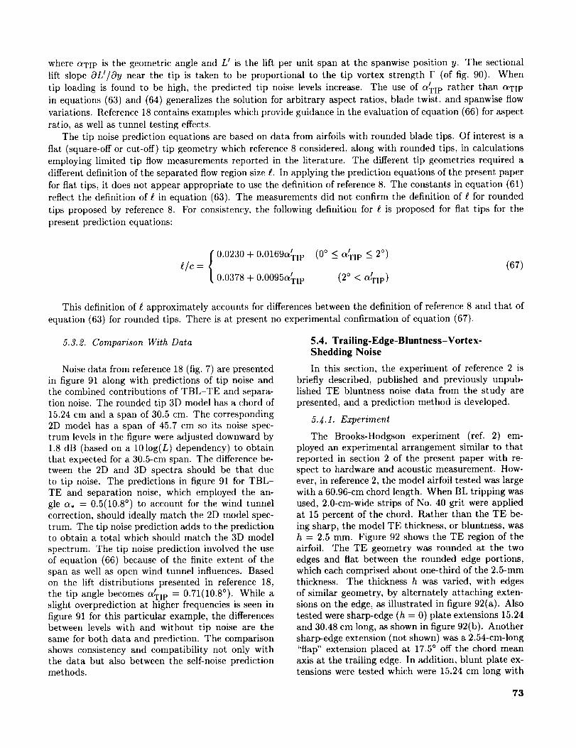
where O_TiP is the geometric angle and L _ is the lift per unit span at the spanwise position y. The sectional
lift slope OL_/Oy near the tip is taken to be proportional to the tip vortex strength F (of fig. 90). When
tip loading is found to be high, the predicted tip noise levels increase. The use of _TIP rather than _TIP
in equations (63) and (64) generalizes the solution for arbitrary aspect ratios, blade twist, and spanwise flow
variations. Reference 18 contains examples which provide guidance in the evaluation of equation (66) for aspect
ratio, as well as tunnel testing effects.
The tip noise prediction equations are based on data from airfoils with rounded blade tips. Of interest is a
flat (square-off or cut-off) tip geometry which reference 8 considered, along with rounded tips, in calculations
employing limited tip flow measurements reported in the literature. The different tip geometries required a
different definition of the separated flow region size/?. In applying the prediction equations of the present paper
for flat tips, it does not appear appropriate to use the definition of reference 8. The constants in equation (61)
reflect the definition of _ in equation (63). The measurements did not confirm the definition of f for rounded
tips proposed by reference 8. For consistency, the following definition for 8. is proposed for fiat tips for the
present prediction equations:
0.0230 + 0.0169o_I P (0 ° < oz_i p _< 2° )f/c = (67)
0.0378 + 0.0095o_?ip (2 ° < c_?ip)
This definition of _ approximately accounts for differences between the definition of reference 8 and that of
equation (63) for rounded tips. There is at present no experimental confirmation of equation (67).
5.3.2. Comparison With Data
Noise data from reference 18 (fig. 7) are presented
in figure 91 along with predictions of tip noise andthe combined contributions of TBL TE and separa-
tion noise. The rounded tip 3D model has a chord of
15.24 cm and a span of 30.5 cm. The corresponding
2D model has a span of 45.7 cm so its noise spec-
trum levels in the figure were adjusted downward by
1.8 dB (based on a 10 log(L) dependency) to obtain
that expected for a 30.5-cm span. The difference be-tween the 2D and 3D spectra should be that due
to tip noise. The predictions in figure 91 for TBL-
TE and separation noise, which employed the an-
gle _, = 0.5(10.8 °) to account for the wind tunnel
correction, should ideally match the 2D model spec-
trum. The tip noise prediction adds to the predictionto obtain a total which should match the 3D model
spectrum. The tip noise prediction involved the use
of equation (66) because of the finite extent of thespan as well as open wind tunnel influences. Based
on the lift distributions presented in reference 18,
the tip angle becomes o_i P -- 0.71(10.8°). While aslight overprediction at higher frequencies is seen in
figure 91 for this particular example, the differences
between levels with and without tip noise are the
same for both data and prediction. The comparisonshows consistency and compatibility not only with
the data but also between the self-noise predictionmethods.
5.4. Trailing-Edge-Bluntness-Vortex-Shedding Noise
In this section, the experiment of reference 2 is
briefly described, published and previously unpub-lished TE bluntness noise data from the study are
presented, and a prediction method is developed.
5.4.1. Experiment
The Brooks-Hodgson experiment (ref. 2) em-
ployed an experimental arrangement similar to that
reported in section 2 of the present paper with re-
spect to hardware and acoustic measurement. How-ever, in reference 2, the model airfoil tested was large
with a 60.96-cm chord length. When BL tripping was
used, 2.0-cm-wide strips of No. 40 grit were applied
at 15 percent of the chord. Rather than the TE be-
ing sharp, the model TE thickness, or bluntness, wash = 2.5 mm. Figure 92 shows the TE region of the
airfoil. The TE geometry was rounded at the two
edges and fiat between the rounded edge portions,which each comprised about one-third of the 2.5-mm
thickness. The thickness h was varied, with edges
of similar geometry, by alternately attaching exten-
sions on the edge, as illustrated in figure 92(a). Also
tested were sharp-edge (h = 0) plate extensions 15.24
and 30.48 cm long, as shown in figure 92(b). Another
sharp-edge extension (not shown) was a 2.54-cm-long
"flap" extension placed at 17.5 ° off the chord meanaxis at the trailing edge. In addition, blunt plate ex-
tensions were tested which were 15.24 cm long with
73

h = 2.5 and 4.8 mm and 30.48 cm long with h =4.8 mm. These extensions with rounded TE corners
are shown in figure 92(c). Tape, 0.08 mm thick, wasused to provide a smooth surface transition from theairfoil to the extensions.
Presented in figure 93, from reference 2, are powerspectral noise data of the airfoil at four flow veloc-
ities. The airfoil is at zero angle of attack and the
boundary layers are tripped. The microphone ob-server position is re = 1.22 m and Oe = 90 ° with re-
spect to the model trailing edge. For two speeds, the
spectra are given for the four TE thicknesses of fig-ure 92(a). The spectral results for the sharp, h = 0,TE cases should be all due to TBL-TE noise. The
bluntness contributes additively at high frequencies
to the spectrum levels. The values given for h/5*
in figure 93 differ slightly from those specified inreference 2 because 6' here is calculated from the
BL thickness scaling equations of the present paper.
Data are presented in reference 2 for the sharp ge-ometries of figure 92(b), as well as the mentioned
17.5 ° sharp flap extension. These geometries give es-
sentially the same spectra as the sharp extension offigure 92(a). This demonstrates that TBL-TE noise
is rather invariant with regard to geometry changes
in the edge region, as long as the TE is sharp and
the boundary layers are substantially the same.
Trailing-edge bluntness noise spectra in a
smoothed 1/3-octave format are presented in fig-
ure 94 for the edge geometries of figures 92(a) and92(c). These spectra are the result of a spectral
subtraction process between the total spectra andthe corresponding sharp TE spectra and should thus
represent the bluntness contribution only. With the
exception of the eight spectra also represented in
figure 93, the data have not been previously pub-
lished. The indicated values of h/_* for the ex-tensions are based on calculations of _f* for the TE
of the airfoil without the extensions. This is justi-
fied by indications that the boundary layers did not
substantially change over the zero pressure gradient
extension plates due to the influence of the upstream
adverse pressure gradient (ref. 2). The spectrum for
the airfoil with h = 2.5 mm and h/_* = 1.15 in fig-
ure 94 is for naturally transitional boundary layers;all others are for tripped boundary layers.
5.4.2. Scaled Data
The spectra of figure 94, as well as limited fre-
quency data of Blake (ref. 19), form the foundation
of the scaling approach. As with the scaling ap-
proach for TBL-TE and LBL-VS noise, the level,
frequency, and spectral shape are modeled as func-
tions of flow and geometric parameters. For the level
and frequency definition, we chose the peak of the
74
spectral humps as the reference. The peak value ofStrouhal number, defined as
Sdtt - fpeakh (68)_peak U
is plotted versus the thickness ratio h/6* in fig-ure 95. The Strouhal numbers increase with increasesin thickness ratio. The Strouhal numbers for the
plate extensions of figure 92(c) are uniformly higher,
for the same thickness ratios, than for the edge ex-tensions of figure 92(a). Also shown are two results
• obtained from Blake (ref. 19). Blake presents sur-
face pressure data for a large array of plate edge
geometries all for very large values of h/6* (with
the exception of the ref. 2 data reported and the one
case shown in fig. 95 at h/6* = 5.19). Blake, for most
data, employed Strouhal relationships which dependon special wake stream thicknesses, and convectionvelocities not available without measurements. From
Blake, however, it is obvious that different TE ge-ometries have different frequency dependences, con-
sistent with the result of figure 95 that Strouhal num-bers for the flat plate extension and the airfoil TE
geometries differ. The primary difference betweenthe geometries is that the NACA 0012 airfoil has a
beveled or sloping surface upstream of the trailing
edge with a solid angle • of 14 ° and the flat plate
has q2 = 0°. The result shown from Blake in fig-ure 95 at hi6* = 5.19 is for a plate with ko = 12.5 °
and nonrounded TE corners. In figure 95, parallel
curves are fitted to the data. The curves, designatedwith values of _, are defined on the basis of a match
point at h/6* = 20 for ko = 0 °. From Blake's scaling
for a thick flat plate (h/6* large) with nonrounded
TE corners, one can determine that fh/U = 0.21
at hi6* = 20. The curve for kO = 14 ° interceptsBlake's k0 = 12.5 ° result, but this is deemed an ac-
ceptable deviation from the curve fit. For scalingpurposes, values of q,Ht for • values other than 0 °'-'_peakand 14 ° could be determined by linear interpolationas described in the calculation procedure section tofollow.
For amplitude scaling, the peak values of the 1/3-
octave spectra of figure 94 were normalized as
M55hLScaled peak SPL1/3 = Peak SPLl/_ - 10 log \ re_ ]
(69)The 5.5 power for Mach number dependence was
determined to give better overall scaling success than
either a 5 or 6 power. Figure 96 shows the scaled
levels plotted versus the thickness ratio h/5*. As
in figure 95 for the Strouhal dependency, the scaledlevels are uniformly higher for the plates than for the
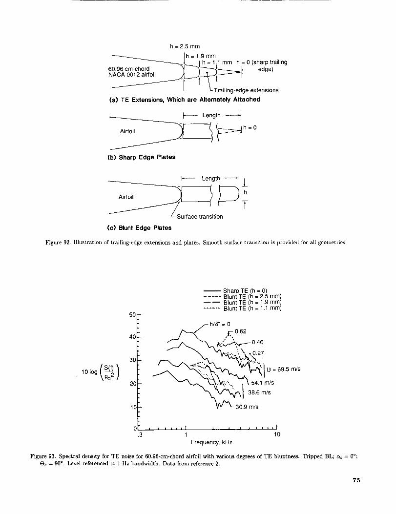
h = 2.5 mm
/h = 1.9 mm.._L | h = 1.1 mm h = 0 (sharp trailing
60.96-cm-chord __,_ edge)NACA 0012 airfoil - _
/ _-Trailing-edge extensions
(a) TE Extensions, Which are Alternately Attached
Airfoil
Length
(b) Sharp Edge Plates
Airfoil
P---- Length ---4 /
Surface transition
(c) Blunt Edge Plates
Figure 92. Illustration of trailing-edge extensions and plates. Smooth surface transition is provided for all geometries.
(S(f)101og \p_ )
50-
4O
30
2O
10
Shard TE (h = 0)..... Blunt TE (h = 2.5 mm)
m Blunt TE (h = 1.9 mm)....... Blunt TE (h = 1.1 mm)
,,__h/5* = 0
/1-_, 0.62,_,,,,.,_,x.v.....- 0.46
,,\
o-, "" _...%.,......
"_" _" U -- 69.5 m/s
Vv • 30.9 m/s
.3 1 10
Frequency, kHz
Figure 93. Spectral density for TE noise for 60.96-cm-chord airfoil with various degrees of TE bluntness. Tripped BL; at = 0%Oe = 90 °. Level referenced to 1-Hz bandwidth. Data from reference 2.
75

100
90
80
70
SPL1/3,dB
60
50
40
30
I I I I I I I I
Plate with h = 4.76 mmLength = 30.48 cm, M = .206,h/5* = 1.16
Plate with h = 4.76 mmLength = 15.24 cm, M = .206,h/5* = 1.16
_ Airfoil with h = 2.54 mm:
M = h/5* =-- .203 1.15
.203 .62m
•181 .60
-- . 158 .56
I I
•135 .55
/ I I I I I I
/", Plate withh = 2.54 mm
i _ Length = 15.24cmM = .206h/5* = .62
I
I
: I Airfoil:
,, I h = 1.g mm
, I M = .203h/,5* = .46 _
"'_h=1.1 mmM .203% =
• h/5" = .27
h = 1.9 mm, !M = . 113, h/5" = .40 "--
.2 1 10 20
Frequency, kHz
Figure 94. TE-bluntness vortex-shedding noise extracted from data of figure 93, data for untripped BL, and data with plate
extensions (fig. 92(c)) attached.
76
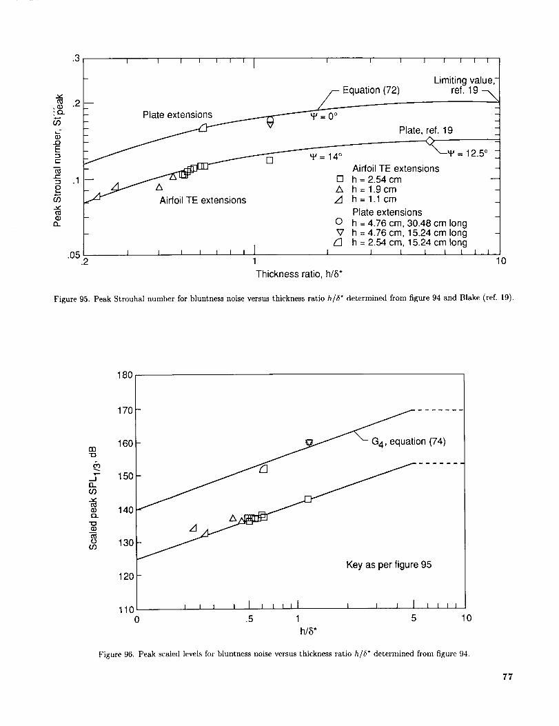
"4
"Q..
03
E"1
c-
t-
"I
£03
13_
.3
.2
.1
I I I I I I I ] I I I i I i I I
_ _ Equation (72)
Plate, ref. 19J_
: _ D _=14 ° "z"'--_ = 12.5°Airfoil TE extensions
_ions
Limiting value,-
ref. 19 -_
[] h = 2.54 cmA h = 1.9 cm/1 h= 1.1cm
Plate extensionsO h = 4.76 cm, 30.48 cm longV h = 4.76 cm, 15.24 cm long
/"] h = 2.54 cm, 15.24 cm longI I I I I I I 1 I I I 1 I I I I
1
Thickness ratio, h/5*
Figure 95. Peak Strouhal number for bluntness noise versus thickness ratio h/tf* determined from figure 94 and Blake (ref. 19).
180
170
m 160"O
_ 150D_O3
140El.
o 13003
120Key as per figure 95
110 [ _ _ _ I _ _I _ J J I _ _0 .5 1 5
h/5*
0
Figure 96. Peak scaled levels for bluntness noise versus thickness ratio hi6* determined from figure 94.
77

edgeextensionsfor thesamethicknessratios. Thelevelsincreasewith increasingthicknessratios. Theedgeextensiondata for the twosmallerthicknessesof h = 1.1 and 1.9 mm at M -- 0.113 deviate most
from a straight line trend. Because of signal-to-
noise concerns in the specification of these points,
these data have the least confidence in the figure
and are thus ignored in the specification of a curve
fit. However, the accuracy of the resultant scaling
equations in predicting these data is subsequently
examined. The curve fits, designated as G4(h/5*, _),shown for the data are straight lines which are chosen
to level off at h/_* = 5. The curve fit behavior at
high h/6* is admittedly rather arbitrary, but there
are no noise data available for guidance, unlike in the
above Strouhal scaling where some frequency data
from Blake are used. Fortunately, in practice, the
likely values of h/_* to be found for rotor blades and
5.3.3. Calculation Procedures
wings should be in the range where data are presentand scaling confidence is greatest.
III
Given the specification of the functions Stpeak andG4, a definition of the spectral shape completes the
scaling. Spectral curve fits for the data of figure 94
are shown for the airfoil TE extensions, ko = 14 °, and
for the plate extensions, _ = 0 °, in figures 97(a) and97(b), respectively. The shapes reflect the observa-
tions that the spectra are sharper for the plates for
the same hi5*, and the spectra widen in the lower
frequencies for decreased h/5* values for both theplates and the edge extensions. The spectral curve fit
is specified as the function G5(h/5*, _) whose peaklevel is 0 dB and whose shape is defined in terms ofSt m t m/S peak" The specification of G5 for in-between
values of ko would be an interpolation between the
limiting cases shown in figures 97(a) and 97(b).
The TE bluntness noise spectrum in a 1/3-octave presentation is predicted by
Stm )., (70)
Stpeak
The directivity function D h is given by equation (B1) in appendix B. The Strouhal definitions are (see fig. 95)
Stm= f__hhU (71)
and
( 0.212)- 0.0045k0 ( ) (0.2 < h/fiavg )
-1 -2 -
¢,m 1 + 0.235 h/5_vg - 0.0132 h/f_vg (72)_peak --
0.1(h/6*vg ) + 0.095 - 0.00243k0 (h/6*vg < 0.2)
The h/6avg term is the ratio of TE thickness (degree of bluntness) h to the average boundary-layer displacement
thickness 6avg, where
_avg -- _ + _; (73)2
The angle k0 is the solid angle, in degrees, between the sloping surfaces upstream of the trailing edge. For an
edge on a flat plate ko = 0 °, whereas ko = 14 ° for an NACA 0012 airfoil. The determination for this parameter
for other TE geometries is discussed in section 6 and appendix C.
The peak level of the spectrum is determined from the function G4 (see fig. 96) where
17.51og 157.5 1.114kO (h/6avg < 5)+ -= (74)
169.7- 1.114k0 (5 < h/_avg )
The shape of the spectrum is defined by the function G5 (see figs. 97(a) and 97(b)) where the calculation
procedure involves an interpolation between the spectra for k0 = 0 ° and 14 ° as follows:
(,fv,st., G5 _, _ = (C5)_v=oo + 0.0714k0 [(Gs)g=14o - (G5)_=o o] (75)' Stpeak )
78

10 I ' ' ' ' ' ' ''1 '
I0
= •
(G5)_ = 14o-10
dB
-20
!
-30.1 1
Strouhal ratio, St"'/St'p_ak
I I I ! I t I
(a) • = 14 °.
I I I l i t |
0
(G5),_ = 0o
dB
10
-10
-20 -
-30.1
I I I I I I I I I I
h
/, , /, ,_ I
1
Strouhal ratio, St'"/St'l_ak
(b) • = 0°.
Figure 97. Spectral shape functions for TE bluntness noise.
I I I I I I I
| i i I I I I
10
79

where
I mTl+ k
2.5k//1 - (rl/#) 2 - 2.5(G5)¢=14o
v/1.5625 - 1194.997/2 - 1.25
-155.543_? + 4.375
(7 < 70)
(705 v < o)
(0 < y < 0.03616)
(0.03616 < 7)
(76)
ttt Ill7/= log(St /Stpeak ) (77)
0.1221
-0.2175(h/6_vg ) + 0.1755
-0.0308(h/6_vg ) + 0.0596
0.0242
(h/6avg < 0.25)
(0.25 < h/6avg < 0.62)
(0.62 _< h/6avg < 1.15)
(1.15 < h/5*vg )
(78)
m
68.724(h/6_vg ) - 1.35
308.475(h/6_vg ) - 121.23
224.811(h/6_vg ) - 69.35
1583.28(h/5_vg ) - 1631.59
268.344
(h/6_vg < 0.02)
(0.02 < h/5_vg < 0.5)
(0.5 < h/6_vg < 0.62)
(0.62 < h/6_vg < 1.15)
(1.15 < h/5_vg < 1.2)
(1.2 < h/6:vg )
(79)
and
_/ m2#4 (80)r/0 =-- 6.25+m2# 2
k=2.5 1- -2.5-mr/0 (81)
The spectrum (Gs)_=0o is obtained by computing equations (76) through (81), as one would for (G5)_=14 o,
but replacing (h/6avg) by (h/Savg) I where
h = 6.724 6aX-_g - 4.019 + 1.107(82)
8O
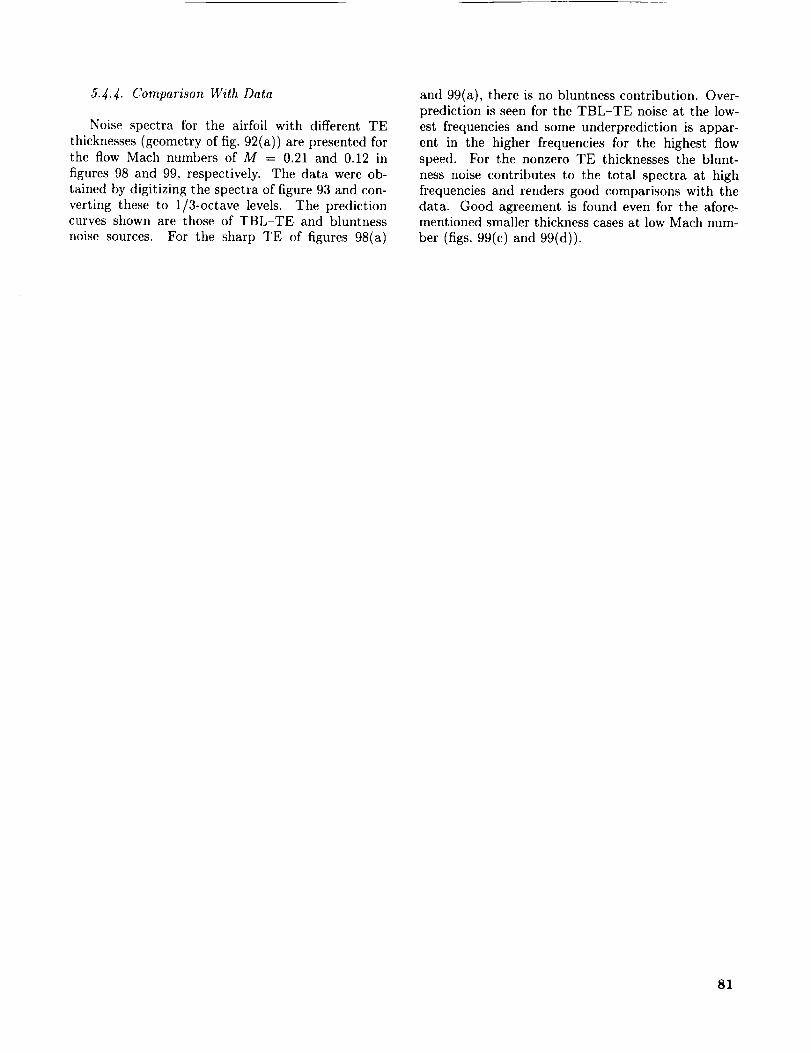
5.4.4. Comparison With Data
Noise spectra for the airfoil with different TE
thicknesses (geometry of fig. 92(a)) are presented forthe flow Mach numbers of M = 0.21 and 0.12 in
figures 98 and 99, respectively. The data were ob-
tained by digitizing the spectra of figure 93 and con-
verting these to 1/3-octave levels. The predictioncurves shown are those of TBL TE and bluntness
noise sources. For the sharp TE of figures 98(a)
and 99(a), there is no bluntness contribution. Over-
prediction is seen for the TBL TE noise at the low-
est frequencies and some underprediction is appar-
ent in the higher frequencies for the highest flowspeed. For the nonzero TE thicknesses the blunt-
ness noise contributes to the total spectra at highfrequencies and renders good comparisons with the
data. Good agreement is found even for the afore-mentioned smaller thickness cases at low Mach num-
ber (figs. 99(c) and 99(d)).
81
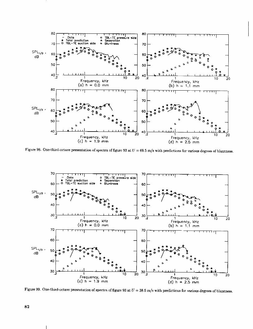
SPLv_ ,
dB
SPLI/3 ,
dB
8O
70
60
5O
40.2
80 j
70--
6O
5O
40 J.2
I I t I I 11 I I I I I I I I I|
- Data o TBL-TE pressure sid__r Totolpred[ction A Sel_oration
-- o TBL-TE suction side ¢_ Bluntness
_o
_*o o
_ v ° ;'Ito w
o,k
_l I I IIIJ I I I I I I II 0 "k
1 10 20
Frequency, kHz
(o) h = 0.0 mm
**o--_ oo
0 0
r_
id, I Illll I I i
1
Frequency, kHz
(c) h = 1.9 mm
m
lit
o _ro_r
?*J I llz 0,t_-
10 20
80
70
60_
50
40.2
80
70
60
50
40 2. J
' ' ' ''"1 ' ' ' ' ''"1
w o o
.;;oOr, 0
r, 0c= 0 "A"
r. 0 _rt_
.= =_ ?*_ -- I I J II, I I I [ I I II 0 _r
1 10
Frequency, kHz
(b) h = 1.1 mm
2O
I
,k,l. "A'_
-,i. ; 0 0 mo o
o r_r_ 0 "A"
-- 0 _rr, 0 "A" --
0 _"
" ?*i I J i,Jl i i _ __ , ttj 0 _
1 10 20Frequency, kHz
(d) h = 2.5 mm
Figure 98. One-third-octave presentation of spectra of figure 93 at U = 69.5 m/s with predictions for various degrees of bluntness.
SPL,/_ ,
dB
SPLva ,
dB
70
60
50
40
I I I I III I I- Data
_) Total prediction-- TBL-TE suction side _ Bluntness
,A, W "R ,k
w O_.A "
;-__oio
o
I I I I I Ill I I I
30.,_ 1
Frequency, kHz
(o) h = 0.0 mm
70 ' ' ' ''''I ' ' '
60--
50,
40
30. _ ' , , , ,,il2
I I I I III I
o TBL-TE pressure sideA Separation
,jo _r
owI I I tD i_r
10
I I III i
-- r, " O_OWr, 0 W
r. 0 _
,o*I I I I I • I'_"
1
Frequency, kHz
(C) h = 1.9 mm
2O
10 2O
70
60
50
40
30.2
70
60
50
40
302
' ' ' .... I ' ' ' ' ''"1
_- _r 'R" 1_..
w O__r
_o)o
r, 0I:1
I @ ' ' lllt I I Ib1
Frequency, kHz
(b) h = 1.1 mm
I I I I I I i I I I I
_r0
0 "_
10
1 1 1111
I
i ° o
P I I I Illl I
1
Frequency, kHz
(d) h = 2.5 mm
_ro _r
o _o _
0 *r_ o _"
10
2O
2O
Figure 99. One-third-octave presentation of spectra of figure 93 at U = 38.6 m/s with predictions for various degrees of bluntness.
82

6. Comparison of Predictions With
Published Results
The scaling law predictions are compared in thissection with data from self-noise studies of airfoil sec-
tions performed at the United Technologies Research
Center (UTRC).
6.1. Study of Schlinker and Amiet
Schlinker and Amiet (ref. 3) conducted tests in
the UTRC Acoustic Research Tunnel to study TBL-
TE noise from a cambered helicopter blade section.The cross section of the 40.6-cm-chord and 53.3-cm-
span model is shown in figure 100. As in the present
NASA Langley studies, the model was mounted on
sidewalls and spanned the width of the open tun-
nel jet, so that the flow across the model was two-
dimensional. The nozzle providing the flow had a
rectangular exit of dimensions of 29 cm × 53.3 cm.To isolate the TBL-TE noise from facility back-
ground noise, a directional microphone system wasused. The experimental configuration, illustrating
the shear layer refraction effect on the TE noise re-
ceived by the directional microphone, is shown in fig-ure 101. The Mach numbers tested ranged from 0.1
to 0.5 and the tunnel angle of attack at varied from
-0.4 ° (zero lift for this cambered airfoil) to 12 °.
6.1.1. Boundary-Layer Definition
Because only TBL TE noise measurements weredesired, the boundary layers were tripped by apply-
ing thin serrated aluminum tape at the blade loca-tions indicated in figure 100. The tape thickness
was on the order of the BL displacement thickness
at the points of application, providing minimum sur-
face protrusion to avoid unnaturally large TBL thick-nesses downstream. This "light" trip is in contrast
to the present study where the trips were "heavy" forreasons discussed.
Hot-wire measurements were made in the
boundary-layer/near-wake region at the TE of the
model. In figure 102, measured BL thicknesses are
plotted versus Mach number for various tunnel anglesof attack at. These data are from figure 17 of refer-
ence. 3. At zero lift, at = -0.4 °, in figure 102(a), the
BL thicknesses 50 on the pressure and suction sides
are approximately the same. This should be expected
since they developed under approximately the same
adverse pressure gradient. Included in figure 102(a)
are corresponding values of BL displacement thick-
nesses, which were calculated by the present authors
from velocity profiles presented in reference 3 (5" wasnot a quantity of interest in ref. 3). In figures 102(b)
and 102(c), 8/c values are shown for at = 7.6 ° and
12 °, respectively. Comparing figures 102(a), 102(b),
and 102(c), one can see that as angle of attack in-
creases, 6s increases and _p decreases.These measurements are compared with the
thickness scaling equations of the present paper.
First, equations (2) and (3) are used to calculate the
BL thickness ratio 8o/c and displacement thickness
ratio _/c. To make the calculations agree with thedata of figure 102(a), all calculated values of 6o/c
and 6_/c were multiplied by a factor 0.6. This factoris taken to be the adjustment in equations (2) and
(3) needed to make them appropriate for the "light"
trip of reference 3. Next, the corrected angles of at-
tack are determined by (1) adding 0.4 ° to at so that
the tunnel angle is referenced to the zero-lift case
and (2) using equation (1), with c = 40.6 cm andH = 79 cm, to obtain a. = 0 °, 3.9 ° , and 6.1 ° for
at = -0.4 °, 7.6 °, and 12 °, respectively. These val-
ues of a. are now used in equations (8) and (11) to
obtain t5p/8O and 8s/t5o, respectively. The resultant
values of bs/c and 8p/c are compared with the datain figures 102(b) and 102(c).
6.1.2. Trailing-Edge Noise Measurements and
Predictions
Trailing-edge noise spectra in a 1/3-octave pre-
sentation are given in figure 103 for the airfoil at
at = -0.4 ° with Mach number ranging from M =0.1 to 0.5. The data were obtained by the direc-
tional microphone system at differing orientations to
the airfoil. Shear layer corrections and directional
microphone gain adjustments were made so that the
data shown represent the noise radiated from a unit
length of L = 0.3048 m of the TE span, at an ob-server distance of re = 3 m, and an observer angle
be which is specified in the figure. Figures 104 and105 contain spectra for the airfoil at at = 7.6 ° and
12 ° , respectively.
The TBL-TE and separation noise spectra were
predicted using the calculation procedures of the
present paper. The values of a., 8_, and 6p usedwere calculated as described in the previous section.
Because of the BL trips and the 2D flow, no LBL-VS
or tip noise calculations were made. In performingthe calculations for TE bluntness noise, one has to
assign values of the TE thickness h and the TE flow
angle parameter _. The thickness was indicatedin reference 3 to be h = 0.38 mm but the shape
of this small TE region was not given. A value of= 17 ° has been used in the prediction because it
gives reasonable prediction-data comparisons.
In figures 103 to 105, the predictions are com-
pared with the measurements. As in the presentationof figures 11 to 74, the individual noise contributions
are shown, along with the total summed spectra.
The prediction-data comparisons are good, especially
83
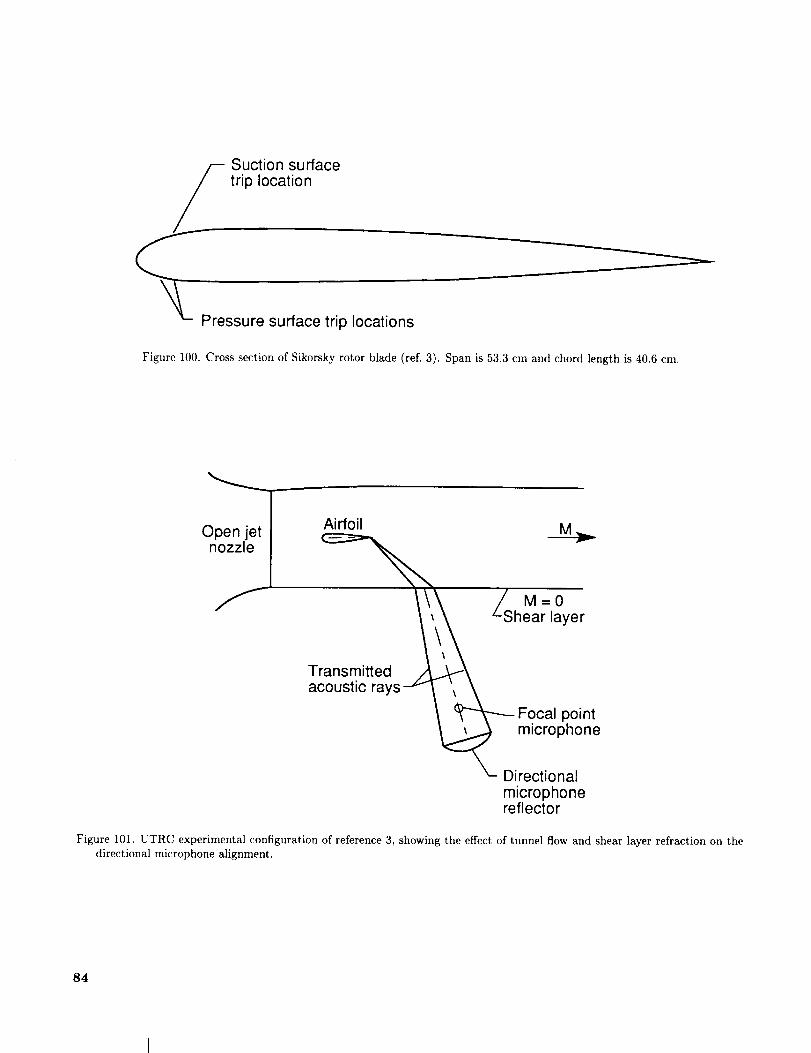
Figure 100. Cross section of Sikorsky rotor blade (ref. 3). Span is 53.3 cm and chord length is 40.6 cm.
Open jet Airfoilnozzle
M=Of 4hear layer
T
acoustic rays -J_/ '_.._...__ Focal point
microphone
_- Directionalmicrophonereflector
Figure 101. UTRC experimental configuration of reference 3, showing the effect of tunnel flow and shear layer refraction on the
directional microphone alignment.
84

_0 _0
c c
.05
.04
.03
.02
.01
0
.05
0 Pressure side
[] Suction side0.6 of that calculated from
equations of section 3
'°'c
50/c
(a) o_t= -0.4 ° (o_, = 0 °)
C
6C
.04
.03
.02
.01
i5s/C..._____I1 _FL
.05
.04
.03
.02
.01
©
I I I I
(b) oct = 7.6 ° (o_, = 3.9 °)
5s/c [] []
5p/C C) 0 00
o I I I I0 .1 .2 .3 .4 .5
Mach number, M
(c) oct= 12 ° (o_, = 6.1 °)
Figure 102. Measured boundary-layer thickness at the TE of the Sikorsky airfoil (ref. 3). Comparison is made with scalingequation results of present paper, multiplied by 0.6 to account for light trip condition.
85
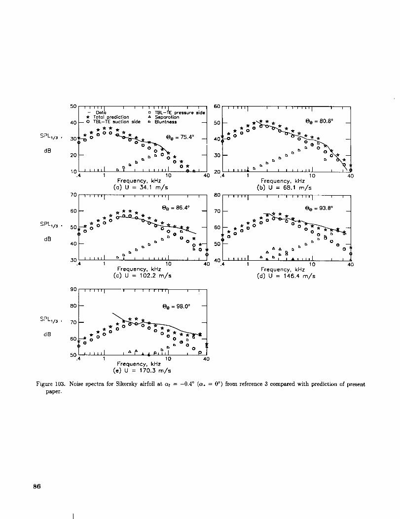
SPLI/_ ,
dB
SPLII3 ,
dB
50 , _,HIO- Dot_r ToIol prediction & Seporotion
40 -- 0 TBL-TE suction side " Bluntness
_o:*** ° __=7s4o20 -- r. " 0 _ _.
r. 0I I IIll 5 II_ I I I I IIll OW
10 4 _ _ i. 1 10Frequency, kHz
(0) U = 34.1 m/s
70 ' ''''I ' ' ' ' ' '"I ' '
e e = 86.4 °60-- __
_,o
50,-_ 0
b _ 0 _r
40 --
I I I III
30.4 1
' ' ' '""_ ' 't
a TBL- E pressure side
40
iI I I I I I III
10Frequency, kHz
(c) U = 102.2 m/s
oo,w-b 0
I I
4O
60 ' ''"I ' ' ' ' ''"I ' '
50 -- .'.tL*. ee = 80.8 ° --
*o*O_.
4o-;*° -_ -,30 _ b t_ _" - 00_ --
_,, _,. 13 B r,, % "t
I I I I I
20.4 _. _' I i i i i ilil i i\i)1 10 40Frequency, kHz
(b) U = 68.1 m/s
80 ' ''"I ' ' ' ' ''"I ' '
70 -- Oe = 93"8° --
_ro060 " _ o C;o
t_ u
50 ,, _" O0 --A t, r, 0
40 , , ,l,l " " , a , ,,,l i i.4 1 10 40
Frequency, kHz(d) U = 146A m/s
SPLv3 ,
dB
90|,' '''1 ' '''' '''1 ' !|
8of o=o8.oo170 ¢r_ --t
0oo.,,o-..50, , ,,J,l , , • _ Pi,,l , P/
.4 1 10 40Frequency, kHz
(e) U = 170.3 m/s
Figure 103. Noise spectra for Sikorsky airfoil at at = -0.4 ° (a, = 0°) from reference 3 compared with prediction of present
paper.
86

SPLI/5 ,
dB
SPLI/3 ,
dB
50 I I I I I I I I I I I I Ill I- DotI a TBL- E pressure_r Total prediction A Separation
40 - ORT(_J_-TEsuction side " Bluntness
30- a _ Oe = 75-4°
n°°20 - . o o o_
.4 1 10Frequency. kHz
(o) U = 34.1 m/s70 ' ''''1 ' ' ' ' ''"1 '
6O
5O _
40 _
-30.4
I
side
I
A* A*. _ ee = 86.4 °
-- o o[] oo_-D° A ,."_ o[]8
,, @_ 0
, Jl,II - _l . , ,_.,,I , o p1 10 40
Frequency, kHz(c) U = 102.2 m/s
60 ' ''''1 ' ' ' ' ' '"1 ' '
_40 'L- [] ° [] A _ _ _
o o - "" 0 _B=_,_
Z_ O _ 0 o"%_ --
30 _. ,, R, O O -'_[_r_ A
,,,,,I_, b , , , , i,,,l c_ , o,40 20.4 1 10 40
Frequency. kHz(b) U = 68.1 m/s
B0 ' ''''1 ' ' ' ' ' '''1 ' '
70 - _. ee=93.8 °
; ; o
50-0 ° ,, ,. o _ o:a B-r, 0
,,,ill I .P , ,,..,I , o404 1 10 40
Frequency. kHz(d) U = 146.4 m/s
SPLv_ ,
dB
90 ' ' '''I ' ' ' ' ' '"I ' '
80 - ee = 98.0 ° -
."IF¢..
*goo_70 - --
,, o o °° =: ' __* o*_,_.601 o o - Uo ° B B
Lk O A _ _ 0
so.4,°,,,,t , , , , _,_,,'i' ?,-,,= [1 10 40Frequency, kHz
(e) U = 170.3 m/s
Figure 104. Noise spectra for Sikorsky airfoil at a_ = 7.6 ° (_, = 3.9 °) from reference 3 compared with prediction of present
paper.
SPLt/_ ,
dB
_o ,. '_:,L ' ' ' '. '_,,'-'_,-press're.'ide• " Totolpredlctlon A Separation
60 -- o TBL-TE suction side " Bluntness
50 -8° OOo o_** ee=80.8 ° -
40 -- [] a A u O_,,_l_/_.__t _° o - O = =---_-_.
' , ,,,,I , ,, ,,.,_,T^ ?.-_3o.4 1 - 10 - 40
Frequency. kHz(o) U = 68.1 m/s
80 ' ''"I ' ' ' ' ''"I ' ' II
70 -- _ /_ /_ ee = 86.4° --_t[ /
50-- []o - e __'- \1
, , , , ,;,,,,_ _*_140 4 m 1 10 - 40
Frequency, kHz(b) U = 102.2 m/s
Figure 105. Noise spectra for Sikorsky airfoil at at = 12 ° (a, = 6.1 °) from reference 3 compared with prediction of present paper.
87

considering that the predictions are based empiricallyon a different airfoil section and that the noise mea-
surement methods were quite different. There does
appear to be a mild overprediction of the TBL TE
noise, although not consistently so. The extent of
agreement in the spectra where the TE bluntnessnoise contributes is substantially due to the afore-
mentioned choice of • = 17 ° (the previously used= 14° would result in a contribution about 3 dB
higher than that shown).
6.2. Study of Schlinker
The tests of Schlinker (ref. 26) were similar in
design to that of reference 3, whose measurement
configuration is shown in figure 101. The 2D airfoil
model, however, was an NACA 0012 section (as in the
present study) with a chord length of c = 22.9 cm.Again, the aim of the tests was to measure TBL TE
and not LBL-VS noise. However, no BL trip was
used at zero angle of attack because no LBL VS noise
was identified (except for the lowest speed tested and
those data were not presented). At (_t = 6°, the LBL-
VS noise was pervasive so a trip was placed on thepressure side at 30 percent of the chord to eliminatethe LBL VS noise.
The TE noise spectra at various tunnel velocitiesare shown in figures 106 and 107 for the airfoil at
at = 0° and 6°, respectively. The data were pro-cessed so that the levels shown are for the full airfoil
span of L = 53.3 cm and an omnidirectional observer
positioned at re = 2.81 m and Oe = 90 °. For this air-
foil, the corrected angles of attack, using equation (1)with c = 22.9 cm and H = 79 cm, are a, = 0° and
3.9 ° for at = 0° and 6°, respectively. The predic-
tions shown in figure 106 for zero angle of attack arefor TBL-TE, LBL VS, and TE bluntness noise. The
values of 50 and _ used in the predictions were ob-tained from equations (5) and (6), for an untripped
BL airfoil. The predictions shown in figure 107 for
cq = 6° are for only TBL TE, separation, and TEbluntness noise, since the LBL-VS noise was elim-
inated by the pressure side tripping. The required
values of _ were calculated from equation (14), for
an untripped BL. However, the values of _ were de-
termined from equations (3) and (9), for a tripped
BL and then multiplying the result by 0.6 (to re-flect the "light" trip condition as discussed for the
Schlinker and Amiet study). For the calculations for
TE bluntness noise, there was no guidance from the
paper for the specification of h and ko. A reasonableTE thickness of h -- 0.63 mm was assumed and the
TE flow angle parameter was set at ko -- 23 °, because
it gave good agreement for the high frequencies in fig-ures 106 and 107. The overall agreement between the
total predictions and the data appears good.
88
6.3. Study of Fink, Schlinker, and Amiet
Fink, Schlinker, and Amiet (ref. 27) conductedtests in the UTRC tunnel to study LBL-VS noise
from three airfoil geometries. The untripped BL air-
foil models had an NACA 0012 planform and their
geometries are shown in figure 108. The first had
a constant-chord length of 11.4 cm across the span
while the other two were spanwise tapered, having
linearly varying chord lengths along the span. Of
the tapered airfoils, the first had a taper ratio of 2
to 1 with chord length varying from 15.2 cm down
to 7.6 cm. The other airfoil had a taper ratio of 4 to
1 with chord length varying from 18.3 cm to 4.6 cra.The span was L = 79 cm for all cases. Because the
levels of the LBL-VS noise were sufficiently intense
compared with the tunnel background noise, a direc-
tional microphone system was not used to measure
the noise. Instead, far-field spectra were obtained
with individual microphones placed on an arc of
2.25-m radius about the midspan of the models. The
noise data from reference 27 which are presented
in the present report are all from a microphone forwhich Oe ,-_ 90 °.
Reference 27 presented most noise data in narrow-band form at various bandwidths to allow exanfi-
nation of the tonal character of the LBL VS noise.
To compare these data with the predictions of the
present paper, the narrow-band data were digitizedand converted to 1/3-octave presentations. As a
check on this procedure, as well as a check on the con-
sistency of the data presented in reference 27, overall
sound pressure levels (OASPL) were computed from
the digitized data and compared with overall levels
reported from direct measurernent. The values gen-erally agreed to within 1.0 dB.
For the constant-chord airfoil at at = 4 °, 1/3-octave spectra are shown in figure 109 for various
tunnel velocities between U = 37 m/s and 116 m/s.The number of spectral bands, as well as the fre-
quency range, presented for the spectra varies for the
different speeds. This variation is due to the differ-
ent narrow-band analysis ranges used in reference 27,
as all available data were used to generate the 1/3-
octave band spectra. For U = 37 m/s, figure 109(a),
the spectrum is fiat at the lower frequencies but ispeaked between 1 and 3 kHz. From the narrow-band
presentation of reference 27 (fig. 22), one finds that
the fiat portion is dominated by broadband noise,
which is characteristic of tunnel background contam-
ination. It is noted again that these spectra are singlemicrophone results from which the background noise
has not been subtracted. The spectral peak region
is due to the presence of three quasi-tones, repre-senting the LBL-VS noise portion. At U = 52, 64,

SPL1/3 ,
dB
60 I I I I I I I I I I I I I I I
- Dot " TBL- E pressure side• " Totol pred[ctlon " Separation
50 _" 0 TBL-TE suctlon side 0 LBL-VS" Bluntness
_r oO "Or
r_ 0 _Ob _ _ O
201 i _llll A I I I I I IIII I..4" 1 " 10 40
Frequency, kHz
(o) U = 44.3 m/s
' ' '"1 ' ' ' ' ' '"1 '70
60--
50
40
3Q.4
*- . *oO°: : 8o:'
_" _r ; 0 r_ O.koO ,_ _ o__r 0 e r. b0 =,
, _,?II i i .'t" ' , ,,,I iI 10
Frequency, kHz
(c) U = 74.9 m/s
I
o:-(
I40
60 ' ''"1 ' ' ' ' _'"1 '
5o- .40 ,_o 0,k; O
r_ O
30"0 " " 0 0
204 1 10
Frequency, kHz
(b) U = 61.5 m/s
o¢r
40
70 ' ''"1 ' ' ' ' ''"1 ' '
60--
_. O OO b b 00#/toO ,-, 00_
4 "A'O _ r_
O_ro _,
30 I I_l lllll [ I I I I IIII I I
.4 1 10 40
Frequency, kHz
(d) U : 91.9 m//s
80 ' ' '''1 i ' ' ' ' '''1 ' '
70
SPLI/_ ' 60 -- ,A- -A" _ ,A, --dB 50 * * 0 o o w'-
w 0 0_. o b (
404 , p,,,& " , , , ,,,ill , ,. 1 10 40
Frequency, kHz
(e) U = 105.5 m/s
Figure 106. Noise spectra for NACA 0012 airfoil at c_t = 0 ° (a, = 0 °) from reference 26 compared with prediction of present
paper.
89

SPLI/3 ,
dB
SPL1/_ ,
dB
60 i i lwl / i I i- Dot
•- Totolpredlct_on50 _ o TBL-TE suct;on side t_ Bluntness
40 -- _r
o ° a "%0*"• o._ . . ._,,s*
20.4_ I lllll _-- ' ± ' ' _"'-_10
Frequency, kHz(o) U = 30.6 m/s
70 ' ' '''l ' ' ' ' ' '''l
60 --
I I I I I| I I
o TBL-?E pressure side
A Seporo|ion
i
40
5o- -4o_ _ A o ° _ It _r,,_ _
[] i_
30.4 _ _, ,,I . _ , , , , J la, l , ___1 10 40Frequency, kHz
(c) u = 61._ m/s
60 ' ' '_'1 ' ' ' ' ' '"1 ' '
50-
4o -
30 -- _ o r , _ _ _ _ro 8*A o - li O
, ,,_,_' , , ; , ,,,,I , o_"20.4 1 10 40
Frequency, kHz(b) U = 44..3 m/s
70, '''''I ' ' ' '''''I ' '
60
5o
40_- ° g []0 _ o b _, O
3o--' _' _'_ _ ' , , ,,,,,t l
.4 1 10Frequency, kHz
(d) U = 74.9 m/s
O oo
i i4O
SPL1/3 ,
dB
80 ' ' '''I i ' ' ' ' '''I '
70 --
60--
:oO0
, __,?,I • ", , , i ,,,I40.4 1 10
Frequency, kHz
(e) U = 88.5 m/s
I
m
m
9 _ _W40 40 4
80
70--
60
50
,. P,_,, I =1
..... I ' ' ' ' .... I ' '
o " r, _-*_,u_[] !_ O
P,B I I I I I I III ^ I 0[
10 40Frequency, kHz
(f) u = 105.5 m/s
Figure 107. Noise spectra for NACA 0012 airfoil at at = 6° (a, = 3.9 °) from reference 26 compared with prediction of present
paper.
90

NACA 0012 airfoils11.4-cm constant chord
U _11.4
7.6
2:1 tapered airfoil
5.2
4.6
I..I-
4:1 tapered airfoil
79 =-
Figure 108. Airfoil models of reference 27. All dimensions are in centimeters.
8.3
and 79 m/s, in figures 109(b), 109(c), and 109(d),
the spectra are very peaked because of the dominat-
ing contributions from large numbers (10 to 15) ofLBL-VS quasi-tones. At U = 98 and 116 m/s, in
figures 109(e) and 109(f), the spectra are less peakedbecause of a somewhat decreased number of quasi-
tones which become submerged within broadband
background noise (which itself increases with speed).
The strong velocity dependence of the noise is
seen clearly in figure 110 (from fig. 25 of ref. 27)
where the OASPL is plotted as a function of veloc-
ity. The overall levels were directly measured, for thenoise between 200 Hz and 20 kHz, rather than deter-
mined by integrating measured spectra. The levelsrise and then stabilize with increases in velocity. The
resumed increase in levels at the highest speeds (ap-
proximately 100 m/s) is where the background noise
appears to become dominant.
Compared with the data in figures 109 and 110
are noise predictions of LBL-VS, TBL-TE, and sep-aration noise. No consideration was given to blunt-ness noise because of the lack of information about
the TE geometry as well as the fact that LBL VS
noise dominates the predictions where comparativedata are available. For the BL thickness determina-
tions, the equations of section 3 for untripped bound-
ary layers were used. The corrected angles of attackwere calculated from equation (1), with c -- 11.4 cm
and H = 53 cm, which rendered a. = 0 ° and 1.9 °
for at = 0° and 4°, respectively. These were em-
ployed with the prediction equations for an observerat re = 2.25 m, Oe = 90 ° , and (be = 90 ° . The
predictions in figure 109 give good comparisons, ex-
cept that the peak frequencies are lower than pre-
dicted. The previously described background noisecontributions explain the differences for the lowest
and highest speeds. For the predictions of OASPL in
figure 110, the spectra for LBL VS, TBL-TE, and
separation noise were summed. Predictions are pre-
sented for not only at = 4° but also at = 0°, 2 °, and6 ° . This is done to show the great sensitivity of the
predictions to airfoil angle of attack. It is seen that
the data would most agree with predictions for aboutat _, 5 ° rather than at = 4°. This could be inter-
preted to mean that the agreement is on the order ofpossible experimental bias error in angle definition.
The tapered-chord airfoils were used in refer-
ence 27 to provide a continuous variation in expected
vortex tone frequency to compare with an analogous
rotating constant-chord blade. The tone variation
91

90 . . _
,o__o,_ .'. _,ok I \.. __o . 60
dB 60 ,e 0
1 , t , _40 .4 Frequency, k .
=0. I_ ,.u. ,u (b_ U = 52.0 m/so .4 ] Frequency, kHz "-' ' 1
SPL41s ' 80 80° et -7 ,_
40 _u60_ 4 1 Frequency kHz,
.4 Frequency, kHz (,d) U - 79.0 m/s
(c) U = 64.0 m/s
_I00100 _-' .... I
_, . __oo_ _
s_,. ,oF /. -_ / .1 ._ °.I _' -t 7°t- .__ , "_o, ," ". / i ,o
FrequenCy, kHz* " _o 40 _u4 I (f) 6.0 m/s
60.4 1 Frequency, kHz U = 11
(e) U = 98.0 m/s4° (a, = 1'9°) from reference 27 compared with prediction of present
Figure 109. Noise spectra for constant-chord airfoil at at =
paper.
92

OASPL, dB
110
100
90
8O
70
n n i n I I II
60
50
m m
o 6o_-- Data, o_t = 4 --, h.ll_l__._... _ 40 --
/' Predictions
/ /' /
/ //
/
40 i J i i i i i I
20 100 200
Velocity, m/s
Figure 110. Overall sound pressure level versus velocity for constant-chord airfoil from reference 27 compared with predictions
of present paper.
93

was found not to be continuous; however the ta-
pered models did produce spectra containing a largenumber of peaks spread over a somewhat wider fre-
quency range than those for the constant-chord air-
foil at about the same velocities. In figure 111, 1/3-
octave spectra are shown for the 2-to-1 taper air-foil at at = 4 ° for tunnel velocities between U = 27
and 107 m/s. The data are similar to those for the
constant-chord model, except that the peaks are gen-erally less well defined. In figure 112, corresponding
OASPL variations with tunnel velocity are shown for
at = 4% Also in this figure, OASPL is shown for a
range of velocities where at = 0 °.
The predictions shown in figures 111 and 112 were
obtained by dividing the models into 10 segments of
constant chord (where actual chord length for each
segment varied according to the blade taper), then
making predictions for each segment, and summingon a pressure-squared basis the contributions of each.
Angle-of-attack corrections for each segment were
made by calculating the correction based on the mean
chord (11.4 cm) across the span. This correction
was then applied to the angle of attack for each of
the blade segments. The corrected angles, therefore,
were the same as for the constant-chord model, that
is, a, = 0 ° and 1.9 ° for at = 0 ° and 4°, respectively.
The comparisons between predictions and data for
the 2-to-1 taper airfoil appear about as good as those
for constant-chord comparisons. It appears that the
predictions for OASPL at at = 4° (fig. 112) would
best agree if at ,_ 3.5 ° had been used rather than 4%
This again indicates that agreement is on the order
of possible experimental angle definition error. The
OASPL comparisons for zero angle of attack show
the predicted trends to be quite good but the levelsto be overpredicted by 5 to 7 dB.
In figures 113 and 114 are the data and prediction
comparisons for the 4-to-1 taper model at at = 0°.
The predictions are not as good as for the constant-
chord and the less tapered model, although the datastill fall within a predictive range of at = 2° to 3%One should bear in mind that the flow behavior in
the vicinity of the tapered models would be expectedto deviate from the idealized 2D behavior assumed
to be occurring over the small spanwise segmentsemployed for the predictions. This makes it difficult
to assess the meaning of the comparison deviations
for the tapered models.
94

SPLI/5 .
dB
SPLv5 .
dB
90
80
- Dat a TBL- E pressure side
O_ Total pred|cUon A 5eporotlon-- TBL-TE mucUon side 0 LBL-VS
I I I llll
10
Frequency, kHz
(o) U = 27.0 m/s
'I ........ I
|) I I ' I i i@llI I0
Frequency, kHz(c) U = 40.0 m/s
60
50.4 1
go , ,,,
80--
70--
60--
504 I I I I
m
i i
40
I I
i
i
I I
4O
90 '''"I ' '
80--
70--
50.4 m i i LI_I ' '
90
80
70
60
50.4
I I I Ill I
, i,,,,I10
Frequency, kHz
(b) U = 34.0 m/s
..... I ........ I
t
,,,,,, , , , ,,,,,iI I0
Frequency, kHz(d) U = 52.0 m/s
• I
I I
m
I I
4O
I i
I
I
4O
SPLI/5 .
dB
SPLI/3 ,
dB
tO0
90
I I Ill I
80--
70--
I I fill
60.4 1
100 ''"'I
90--
80--
70 --
Bo ,,,,,I
u u i i mill I i
t, , ,, ,,,i
lOFrequency, kHz
(e) U = 67.0 m/s
I I I 1 f ill I
I I
!_!
I
_)• I
. Im I i
u u i i u iii I i ilOo ' ''''I
90--
80--
70--
60.4 ' ''"I
100 r,,,, I
90 --
80
7O
m i iiii
60.4
t
7"
10
Frequency, kHz(f) U = 79.0 m/s
1 i i i i ill I
I
8 *,. ....... I , . , _, , .... I ,
1 10 40 1 10
Frequency, kHz Frequency. kHz(g) U : 88.0 elm (h) U : 98.0 m/s
Q
t
4O
iI
i i i i lull I I I100 ' ''''1
90--
80--
70--
I I IIII
60.4 1
SPLI/JdB ' $-_e
, F ? ® A,e, I , ,lO 4o
Frequency. kHz(1) U = 107.0 m/s
Figure 111. Noise spectra for 2-to-1 tapered-chord airfoil at at = 4° (a, = 1.9°) from reference 27 compared with prediction of
present paper.
95

OASPL, dB
110
100
9O
8O
7O
I i I I I I I I
6O
5O
o
if
/ o_t = 0 °
Predictions
°OOOoo
=0 °
40 I 1 I I I I I I
20 100 200
Velocity, m/s
Figure 112. Overall sound pressure level versus velocity for 2-to-1 tapered-chord airfoil from reference 27 compared withpredictions of present paper.
96

SPLI/s ,
dB
SPL1/3 ,
dB
90 I I I I I / I I I
°°,Total prediction A Separation
80 TBL-TE suction side 0 LBL-VS
60
50.4 1 10Frequency. kHz
(0) U = 30.0 m/s
I I III I
60--
I I llll50.4 1
90
8O
70
I I I I I Ill I
,e
W_
i _. i,,i,?.10
Frequency, kHz(c) U = 55.0 m/s
I I I I II I I
[] TBL-'#E pressure side
I
4O
I
I
4O
9o ' ''"I
80--
70--
60--
I I IIII
50.4 1
9o, '''"I
80--
70--
60--
50 i,,,,l,4 I
I I I I I III I
IO
Frequency, kHz(b) U = 43.0 m/s
I I I I I I I I I
/2
I
4O
I
"k
10 40
Frequency, kHz(d) U = 61.0 rn/s
SPL1/s ,
dB
SPL1/s ,
dB
I I III I
I I till
1
90
80
70
60
50.4
go ' ''''I
80--
70--
60--
I I IIII
50.4 1
I I I I I I II I
_ri _" , II0,0,,I_
10Frequency. kHz
(e) U = 70.0 m/s
I I I I I I I I I
8
I
*
_r llr_r*O000o _r
**n?,,,?,l 08 ,,10 40
Frequency, kHz(g) U = 88.0 m/s
I I I I I III I9o '''"I
80--
70--
60 --
I I IIII
50.4 1
,It 0
, , _,t' IY#t.,TO.. Y*,40 10 40
Frequency, kHz(f) U = 79.0 m/s
Figure 113. Noise spectra for 4-to-1 tapered-chord airfoil at c_t = 0° (a, = 0 °) from reference 27 compared with prediction of
present paper.
97
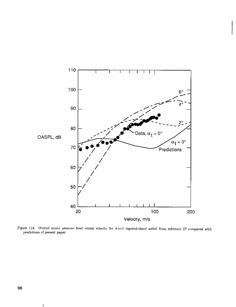
OASPL, dB
110
100
9O
8O
7O
I I
60
5O
I I J I II
ata, o_t = 0 °
a t = 0 °
Predictions
40 J I i l I iiI20 100 200
Velocity, m/s
Figure 114. Overall sound pressure level versus velocity for 4-to-1 tapered-chord airfoil from reference 27 compared with
predictions of present paper.
98

7. Conclusions
This paper documents the development of an
overall prediction method for airfoil self-noise. The
approach is semiempirical and is based on previoustheoretical studies and data from a series of aero-
dynamic and acoustic tests of isolated airfoil sections.
The acoustic data processing employed a correlation
editing procedure to obtain self-noise spectra uncon-
taminated by extraneous noise. Five self-noise mech-
anisms, each related to specific boundary-layer phe-nomena, are identified in the data and modeled. For
each mechanism, the data are first normalized by fun-
damental techniques using scaled aerodynamic pa-rameters. The spectral shape, level, and frequencies
are then examined and modeled for dependences on
parameters such as Reynolds number, Mach number,
and geometry.
The modeling accuracy of the resulting self-noise
prediction methods is established by comparing pre-dictions with the complete data base. The methods
are shown to have general applicability by compar-
ing predictions with airfoil self-noise data reported in
the literature from three studies. A successful appli-
cation of the methods is reported for a large-scale-model helicopter rotor broadband noise test.
Conclusions can be drawn regarding the spe-cific self-noise mechanisms. For the turbulent-
boundary-layer trailing-edge noise and separationnoise sources, an accurate and generally applica-
ble predictive capability is demonstrated, especially
for the important conditions of high Reynolds num-
ber and low to moderate angle of attack. The
mechanism which can dominate the spectra for low
Reynolds number, laminar-boundary-layer-vortex-
shedding noise, is also demonstrated to have good
predictive capability. For this quasi-tonal noise
mechanism, there are some issues, not fully ad-
dressed herein, about how to apply the formulationsin the most appropriate way to different airfoil ge-
ometries. The tip vortex formation noise source ap-
pears to be well predicted, although its relative lack
of importance compared with the other self-noise
sources prevents a full assessment of accuracy. The
trailing-edge-bluntness-vortex-shedding noise sourceis shown to be very important and predictable by the
method developed. For this source, there is an asso-
ciated "flow angle" parameter which is found to be
constant for any given trailing-edge geometry, butis difficult to determine a priori. However, for ap-
plication of the bluntness noise prediction method,
reasonable estimates for this parameter can be made
based on the examples in this report.
The unique prediction capability presented should
prove useful for the determination of broadband noise
for helicopter rotors, wind turbines, airframe noise,
and other cases where airfoil shapes encounter low-
to moderate-speed flow. For modern propeller de-
signs, the present equations should be applied with
some caution because the high-speed, high-loading,
and skewed-flow conditions existing about propeller
blades do not match the low- to moderate-speed and
generally 2D flow conditions of the present data base.
The computer codes given herein can be readily in-
corporated into existing or future noise predictioncodes. The documentation provided in this report
should provide the means to evaluate where and how
any needed future refinements can be made in the
prediction codes for particular applications.
NASA Langley Research CenterHampton, VA 23665-5225April 19, 1989
99
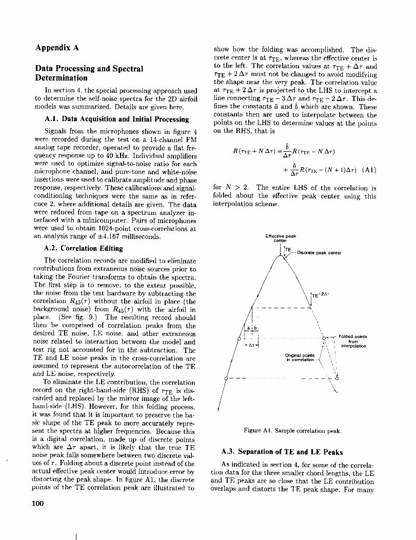
Appendix A
Data Processing and SpectralDetermination
In section 4, the special processing approach usedto determine the self-noise spectra for the 2D airfoil
models was summarized. Details are given here.
A.1. Data Acquisition and Initial Processing
Signals from the microphones shown in figure 4were recorded during the test on a 14-channel FM
analog tape recorder, operated to provide a fiat fre-
quency response up to 40 kHz. Individual amplifiers
were used to optimize signal-to-noise ratio for eachmicrophone channel, and pure-tone and white-noise
insertions were used to calibrate amplitude and phase
response, respectively. These calibrations and signal-conditioning techniques were the same as in refer-
ence 2, where additional details are given. The datawere reduced from tape on a spectrum analyzer in-
terfaced with a minicomputer. Pairs of microphoneswere used to obtain 1024-point cross-correlations at
an analysis range of +4.167 milliseconds.
A.2. Correlation Editing
The correlation records are modified to eliminate
contributions from extraneous noise sources prior to
taking the Fourier transforms to obtain the spectra.
The first step is to remove, to the extent possible,
the noise from the test hardware by subtracting the
correlation R45(r) without the airfoil in place (thebackground noise) from R45(T) with the airfoil in
place. (See fig. 9.) The resulting record should
then be comprised of correlation peaks from thedesired TE noise, LE noise, and other extraneous
noise related to interaction between the model and
test rig not accounted for in the subtraction. The
TE and LE noise peaks in the cross-correlation are
assumed to represent the autocorrelation of the TE
and LE noise, respectively.
To eliminate the LE contribution, the correlation
record on the right-hand-side (RHS) of 7"TE is dis-
carded and replaced by the mirror image of the left-
hand-side (LHS). However, for this folding process,
it was found that it is important to preserve the ba-
sic shape of the TE peak to more accurately repre-
sent the spectra at higher frequencies. Because this
is a digital correlation, made up of discrete pointswhich are AT apart, it is likely that the true TE
noise peak falls somewhere between two discrete val-
ues of T. Folding about a discrete point instead of the
actual effective peak center would introduce error by
distorting the peak shape. In figure A1, the discrete
points of the TE correlation peak are illustrated to
100
show how the folding was accomplished. The dis-
crete center is at VTE, whereas the effective center is
to the left. The correlation values at TTE + Av and
rTE + 2 AT must not be changed to avoid modifyingthe shape near the very peak. The correlation value
at rTE + 2 AT is projected to the LHS to intercept a
line connecting TTE -- 3 Av and 7TE -- 2 AT. This de-fines the constants _ and b which are shown. These
constants then are used to interpolate between the
points on the LHS to determine values at the pointson the RHS, that is
R (r_rE + NAt) =b--_---RAr (rTE-- NAt)
+ _--_rR (TTE -- (N+ 1)AT) (A1)
for N > 2. The entire LHS of the correlation is
folded about the effective peak center using thisinterpolation scheme.
Effective peak
center
center
TTE+2AT
/_ FoldedfromPOintsinterpolation
Or mlig" a points_ _
in correlation _ _, /i
Figure A1. Sample correlation peak.
A.3. Separation of TE and LE Peaks
As indicated in section 4, for some of the correla-
tion data for the three smaller chord lengths, the LEand TE peaks are so close that the LE contribution
overlaps and distorts the TE peak shape. For many

suchcasesa procedurewasfoundto successfullyre-movethe distortionprior to implementingthe TEpeakfoldingprocessdescribedabove.Thisprocedureisexplainedbywayofexampleforthe5.08-cm-chordairfoilshownin thebottomtraceof figureA2. Thepredictedlocationsof theTE andLE noisepeaksinthecorrelationsareindicatedandagreewellwith thepeaksin theactualtrace.Notetheproximityof thetwopeaks.
The procedureto separatethesetwo peaksin-volvescombiningthe originalR45(r) at the bottom
of figure A2 with time-shifted versions of itself, so
that the peaks are separated by larger time delays.
The procedure depends on the implied symmetry of
the LE and TE peaks, inherent in the assumption
that they represent the autocorrelations for the LE
and TE noise, respectively. The first step is to invert
R45(7) in sign, and reverse it in time, by "flipping"
the correlation about "rLE. The result of combiningthese two curves is seen in the second trace from the
bottom of figure A2, denoted R_5(T ). The two peaksseen here are the original TE noise peak, and an in-
verted TE noise peak at 2"rLE - "rTE. There is someincrease in level and some distortion in the correla-
tion record away from the peaks, as should be ex-
pected. The LE noise peak has been removed, but
the inverted TE noise peak still affects the original
peak at rTE. To remove the inverted peak, the initial
R45(v) must be shifted by 2(TLE- rTE ) and summedwith the previous result. This produces the third
t!
curve from the bottom in figure A2, denoted R45(v ).
The TE noise peak has remained at rTE , while the
LE noise peak is now at 3rLE - 2TTE. The peaks arenow separated in time so that details of each peak
can be seen. Note that as the peaks no longer affect
one another's shape, their basic symmetry is evident.This helps to validate the initial assumption that the
peaks represent the autocorrelations of TE and LE
noise. If the peaks must be further separated, this
procedure can be successively repeated, with the re-
sults of the next two iterations seen in the top twoIll llll
traces of figure A2, R45(r) and R45(r ). It shouldbe noted that only the inner portion of the corre-lation is shown (the correlation was performed for
±4.067 ms). Because of the data record manipula-
tions, much of the outer portions of the correlations
did not overlap and were thus zeroed out.
A.4. Determination of Spectra
Once the correlation records, or their modified
forms after the separation processing, are folded
about the effective peak center, the resulting TEnoise correlations are transformed into spectra of
the noise. Because the correlation record lengths
are reduced by varying amounts (typically 20 per-
cent) because of the editing described above, the use
of fast Fourier transform techniques is not conve-
nient. Instead, regular Fourier transform techniquesare used in an approach based on chapter 9 of ref-
erence 28. In summary, a data window is applied
to the correlation (eq. 9.116, ref. 28) and is used to
provide the real and imaginary portions of the spec-trum (eqs. 9.167-9.168, ref. 28). The resulting cross-
spectra (eqs. 9.172 9.174, ref. 28) are presented in
terms of magnitude and phase.
With the cross-spectra produced, amplitude cor-rections are applied to account for shear layer effects,
using the technique of Amiet (ref. 22), as well as self-
noise directivity effects, which are described in ap-
pendix B. The spectrum for each microphone pairwas corrected to an effective position of 90 ° with re-
spect to the airfoil chord line. The combined effec_ of
both of these corrections tended to be small, with the
corrections for many test conditions being less than1 dB. Since cross-spectra were obtained, the correc-
tions for each of the two microphones involved were
averaged to correct the cross-spectral magnitude.
The results obtained from this method are given
in figure A3 for the example correlation records of
figure A2. Figure A3(a) shows the cross-spectrum
obtained from the correlation of the original R45(_-)
record, which is the bottom curve of figure A2, while
figure A3(b) shows the cross-spectrum obtained after
folding the R45(T) record about the TE noise peak.
Note that the cross-spectral phase ¢ is a partial indi-
cator of how well the cross-spectrum represents the
total TE self-noise. Ideally the phase should vary
linearly with frequency, ¢ = 360°fTTn . The breaks
seen in this phase line and the corresponding spectralpeculiarities indicate regions adversely affected by
contamination, which was not removed by the back-
ground subtraction and, in the case of figure A3(b),the folding process. The contamination from the LE
is seen to primarily affect the cross-spectrum of fig-
ure A3(a) below around 4 kHz. Folding the correla-
tion removes most of this, leaving a dip in the spec-
trum of figure A3(b) at about 1.5 kHz. Figure A3(c)
shows the spectrum for the third curve from the hot-t?
tom in figure A2, R45(r), which is the modified corre-lation after two manipulations have separated the TE
and LE noise peaks. The phase difficulty and spectral
dip at about 1.5 kHz in figure A3(b) are eliminated
in figure A3(c). Figure A3(d) shows the spectrumllll
for the top curve of figure A2, R45(T), which is forfour manipulations. This spectrum is similar to that
of figure A3(c) except for some apparent increase in
contamination at the low- and high-frequency ends.
For the airfoil presented here, a choice was made
to use the spectrum of figure A3(c), based on two
101

.010
0
.010
.010
R45 ('r) 0
.010
.010
-.010-2 2
R45 ('c) R45 ('t) R45 (2'tLE "c)
Predicted I:TE 1 f Predicted I:LE
, I , A 10 , 1 ,-1 0 1
ms
Figure A2. Separation of TE and LE peaks in a cross-correlation. Example is cross-correlation between microphones M4 and M5for the 5.08-cm-chord airfoil with tripped BL. a, = 0°, U = 71.3 m/s.
102

103
separation manipulations, to represent the self-noise.
The lower and upper limits to which the spectrum isbelieved to be accurate are from about 0.8 to 13 kHz.
For the other airfoils of this paper, similar evaluations
of the limits were made and the spectra are cut off
beyond these limits in their presentation, as indicatedin section 4.
To increase confidence, all the 2D airfoil spectra
presented in figures 11 to 74 were found by averagingindependently determined spectra from two micro-
phone pairs. After the shear layer and directivity
corrections were applied, the spectra from the two
microphone pairs generally agreed to within 1 dB.
In tables 1 and 2, the data processing and manip-ulations, and whether the correlations were folded
or not prior to taking the spectra, are specified for
each test case. It is seen that for the three larger
airfoils, no correlation manipulations were needed to
separate the LE and TE correlation peaks. For the
three smaller airfoils, performing two separation ma-
nipulations was advantageous for about a quarter ofthe cases. The table shows that a substantial num-
ber of correlations were not folded. For airfoils at
sufficiently high angles of attack, low frequencies can
dominate the noise. This results in large correlation
humps, rather than the relatively sharp peaks which
are needed in the folding process. For these cases, the
raw cross-correlations are transformed, with only the
background subtraction being performed. Also the
correlations were not folded in the presence of strongLBL-VS noise. This noise can dominate all other
self-noise sources, as well as the LE noise contami-
nation, negating the need for the correlation editing.
This correlation editing would have proved difficult,
in any case, since vortex shedding produces noise at
small bands of frequencies, appearing as damped si-nusoidals in the correlation, which tended to mask
other peaks. The effect of folding the correlation insuch cases was examined, however, and found to have
little effect on the spectra.
104

Appendix B
Noise Directivity
The purpose of this appendix is to define the
directivity functions D h and De, which are employed
in the tunnel noise data processing and proposed
for use in the prediction equations for the self-noisesources.
B.I. Retarded Coordinates
The retarded coordinate system is explained by
first referring to figure B1 where the airfoil is at zero
angle of attack to the tunnel flow. If the velocity
were zero everywhere, sound from the model which
reaches the microphones (M2 is shown) would follow
the ray path defined by the measured distance rm
and angle Ore. But with the velocity in the free jet
equal to U, the ray which reaches the microphones
follows first the radiation angle ®c until it encounters
the shear layer where it is refracted. It emerges at
angle Ot with an amplitude change and travels to the
microphone. The theoretical treatment employed inthis study for the angle and amplitude corrections
is that due to Amiet (refs. 22 and 23). A convenient
reference for the corrected microphone measurements
is a retarded coordinate system where the source
and the observer are at corrected positions. The
angle Oe is referenced to a retarded source position
and a corrected observer position where the distance
between the positions is re = rm. As defined, if
there were no shear layer present with flow extending
to infinity, the center of the wave front emittedfrom the source would be at the retarded source
position when the wave front reaches the corrected
observer position. The retarded coordinates are
equivalent to the emission time coordinates employed
in the literature, for example, see reference 29, for
moving sources and stationary observers. Figure B2
shows a source flyover geometry corresponding tothe open jet wind tunnel geometry of figure B1.
Physical equivalence between the cases is attained by
accounting for the Doppler-related frequency shiftsdue to the relative motion between the source and
observer in one instance and no relative motion in
the other. There are no Doppler-related amplitude
corrections required between the flyover and windtunnel cases as the effect of the flow on the source
definition is already included in the wind tunnelenvironment.
B.2. Directivity Functions
In figure B3, a 3D retarded coordinate system is
defined where the origin is located at the trailing edge
of a thin flat plate, representing an airfoil. The flat
plate is in rectilinear motion of velocity U in direction
of the negative xe axis. The observer is stationary.Trailing-edge noise is produced when boundary-layer
turbulence and its associated surface pressure pat-
tern convect downstream (with respect to the plate)
at a velocity Uc (Mach number Mc) past the trail-
ing edge. If the noise-producing turbulence eddiesare sufficiently small and the convection velocities
are sufficiently large to produce acoustic wavelengths
much shorter than the chord length, the directivity
can be shown to be (based oil analysis of Schlinkerand Anfiet, ref. 3)
-- 2 sin2(O_/2) sin2 ¢_ (B1)Dh(Oe'cbe) "_ (1 + McosOe)[1 + (M - M_) cos O,,] 2
where the h subscript indicates the high-frequency
(or large-chord) limit for D. The overbar on D hindicates that it is normalized by the TE noise ra-
diated in the Oe = 90 ° and Be = 90 ° direction, so
Dh(90 °, 90 °) = 1. For the flyover plane (Be = 90°),
equation (B1) is the same as equation (32a) of ref-erence 3. In reference 3, the equation was compared
favorably with measured airfoil TE noise results, for
limited M and Oe ranges, as well as with previoustheoretical results. The directivity expression used
in reference 2 was found to give virtually identicalresults for low Mach numbers.
Although developed for when the velocity U isparallel to the plate along the xe axis, equation (B1)
can be applied when the plate or airfoil is at an
angle of attack a to the flow. In application (refer
to fig. B3), one should define the angles with respect
to a coordinate system that is fixed with respect tothe airfoil with the xe axis fixed along the chord line,
rather than one where the Xe axis is fixed along the
direction of motion. Note, however, that any analysis
of Doppler frequency shifts (not treated in this paper)
should reference angles with respect to the direction
of motion. Applications of equation (B1) at anglesof attack should result in little additional error to
that already built into the relation. Because it was
derived with the plate assumed to be semi-infinite
Dh becomes inaccurate at shallow upstream angles
(Oe ---* 180°), when applied to finite airfoils even
for high frequencies. As frequency is lowered, the
wavelengths become larger with respect to the chordand the directivity becomes increasingly in error.
However, D h should be of sufficient accuracy todefine the directivity of all the self-noise sources
discussed because of their high-frequency character.
The one exception to this is the stalled-airfoil noise.
When the angle of attack of the airfoil is increased
sufficiently, the attached or mildly separated TBLflow on the suction side gives way to large-scale
105

Ray Path 5 _
Ray Path 1_
Ray Pat
vRetarded /Source
/ \_ Positiort _ Corrected_.. I \ / Observer
r "_ \__E)., !@ Position
-'_.__ _y.,_Path 2
IV -Shear Layer
tltff u:oI u=uI
Figure B1. Sketch of shear layer refraction of acoustic transmission paths.
Position of Source Position of Source
at Reception Time _7 F at Emission Time 1"*
° -- - Path Taken by
U(t-T*) 4_ Moving Source
_r e = C o (t-T*)
_ Observer at
Reception Time t
Figure B2. Emission from a source moving with a constant velocity.
106

Plate moves atvelocity U
Z e
/%.
\
/ %.%.
/\
/ %.
// )l Stationary
/ I "_ observer/ / /
/ t // / /
/ I /,I
f/ I
/ t /
/_We
Ye
Figure B3. Flat plate in rectilinear motion.
separation. The turbulence eddies are then compa-rable in size to the airfoil chord length and the eddie
convection speeds are low. The directivity for this
low-frequency noise is more properly defined as that
of a translating dipole, which is
sin 2 Oe sin 2 (I)e
Dt(0e' J)e)_ (1 + M cos ee) 4 (B2)
where the _ subscript indicates a low-frequency limit.
The coordinate system and comments about an-
gle definitions in equation (B1) apply also in equa-
tion (B2). Equation (B2) is employed for the di-
rectivity in the expression for stalled flow noise
(eq. (30)).
For the noise data reduction in the present study,
equation (B1) was used in the determination of the
self-noise spectral levels for the reference observer po-sition, at re = 122 cm and Oe = 90 ° • First, shear
layer refraction corrections were calculated to deter-
mine the spectral level adjustments, to add to mea-sured values, and a resultant source-observer location
at re and (_e. This was done while keeping track of
the actual physical coordinates of the trailing edge
which varied with airfoil angle of attack. Finally,
equation (B1), with (I) = 90 ° and an assumed con-vection Math number of Mc _ 0.8M, was used to
determine final level adjustments required to match
results to the Oe = 90 ° location.
107

Appendix C
Application of Predictions to a Rotor
Broadband Noise Test
An acoustics test of a 40-percent scale model
BO-105 helicopter main rotor was conducted in the
German-Dutch Wind Tunnel (DNW). Figure C1
shows an overview of the test setup in the large openanechoic test section. The 4-meter-diameter rotor is
shown positioned in the flow between the nozzle on
the right and the flow collector on the left. A key aim
of the test was to produce a large benchmark aero-acoustic data base to aid and verify rotor broadband
noise prediction. In reference 30, the present authorscompared data with predictions of rotor broadband
self-noise for a number of rotor operating conditions.The predictions employed the self-noise prediction
methods, which are documented in section 5 of the
present paper, and the NASA ROTONET program(ref. 31) to define rotor performance and to sum con-
tributions of noise from individual blade segments.In this appendix, the experiment is not reviewed
in detail nor are data-prediction comparisons pre-
sented, as reference 30 is complete in this regard.
Rather, reference 30 is complemented by specifyinghow the self-noise prediction methods of the present
paper were applied. Given below is a summary ofthe rotor prediction method, a definition of the rotor
blade geometry and test modifications and a specifi-cation of input parameters for the individual source
predictions. The degrees of success of data-prediction
comparisons in reference 30 are discussed along withrecommended refinements to the prediction methods.
To produce a rotor prediction, the rotor geometry
definition and flight conditions, specified as thrust,
rotor angle, rotor speed, flight velocity, and trim con-dition, are provided as inputs to the ROTONET ro-
tor performance module. The particular module used
assumes a fully articulated rotor with rigid blades
and a simple uniform inflow model. The module de-
termines local blade segment velocities and angles of
attack for a number of radial and azimuthal posi-tions. Ten radial segments were considered at 16 az-
imuthal positions. The BL thicknesses and other pa-rameters needed are calculated. The noise due to
each source is predicted for each blade segment, andthe ROTONET noise radiation module is used to
sum contributions from all blade segments to obtain,after accounting for Doppler shifts and the actual
number of blades, the noise spectrum at the observer.
As indicated in reference 30, the accuracy of
predictions depends on a number of factors includingthe accuracy of the performance module used. One
may question the quasi-steady assumptions used in
108
defining the local BL characteristics, which ignoreunsteadiness and resultant hysteresis effects. Likely
more important is how well the aeroacoustic scaling
determined from low-speed data extends to higher
speed. The Mach number at the tip of the blades is
0.64 for rotor hover, whereas the 2D airfoil modeltests were limited to Mach 0.21. Also there are
questions on how to apply scaling obtained from
symmetrical NACA 0012 sections with particular TE
geometries to the cambered NACA 23012 rotor bladewith different TE geometries.
The model rotor is a 40-percent-scale, four-
bladed, hingeless BO-105 rotor, with a diameter of4.0 m and a chord of 0.121 m. A blade and its details
are shown in figure C2. The blades have -8 ° linear
twist and a 20-percent cutout from the hub center.The effects of several blade modifications were exam-
ined, including (1) application of Carborundum grit
from the blade leading edge to 20 percent chord tomatch the BL trip condition for the 2D blade sec-
tions described in section 2 of the present paper,(2) taping of the TE with 0.064-mm-thick plastic
tape to modify the "step tab" geometry, and (3) at-tachment of a rounded tip to each blade (the stan-
dard blades have a squared-off tip).
C.I. Boundary-Layer Definition
With the local blade segment mean velocities and
angles of attack determined by the rotor performance
module, the equations of section 3 were directly ap-
plied to determine the BL thicknesses required in the
noise predictions. Most noise comparisons in refer-
ence 30 are for the blades with untripped BL. For
the tripped BL, the fact that the BL trip conditionsfor the rotor blades matched the 2D test models as-
sured the appropriateness of using the equations for
a heavy trip rather than modifying the equations as
required for the UTRC comparisons reported in sec-
tion 6. For all BL thickness calculations, the aero-
dynamic angles of attack were used in the equations.
The aerodynamic angle is referenced to the zero lift
angle, which is -1.4 ° from the geometric angle forthe NACA 23012 airfoil.
C.2. TBL-TE and Separation NoisePrediction
Given the definitions of segment chord length,
span width, velocity, aerodynamic angle of attack,and BL thicknesses, the calculation of TBL-TE and
separation noise is straightforward as specified in
section 5. From the data-prediction comparisons ofreference 30, it is concluded that the TBL-TE and
separation noise calculations demonstrated a goodpredictive capability for these mechanisms. The
rotor was tested from hover to moderately high flight

Figure C1. Test setup
am_
L-89-44
m DNW for helicopter main rotor broadband noise study reported in reference 30.
FLAPPINGLAGGING SENSORS
SENSORS -,_ f TORSION SENSOR TIP ROUNDING MOD7
] X__I \ _._ , -_:J"
- ,40"0 '_ :-7_'"'%"_o_'_''" =------- 2000
NACA 23012121mm CHORD
C
TRAILING EDGE MOD
Figure C2. Model BO-105 blade details• All dimensions in mm.
109

speeds for various climb and descent rates at differ-ent thrust settings. Diagnostics included 1/2 rotor
speed tests and the BL tripping tests. It is noted that
the TBL TE and separation noise predictions for anumber of rotor conditions fell below contributions
of LBL-VS, especially at the 1/2 rotor speed, and of
TE bluntness noise. This represents a limitation of
the comparisons which prevents sweeping statements
regarding predictive accuracy of TBL-TE and sepa-
ration noise sources. Still the agreements were quite
good except when the rotor operated at full speed
(tip speed of M = 0.64) and the boundary layerswere tripped. Then the noise was underpredicted by
about 6 dB. It is believed that for this high speed the
heavy trip disturbed the flow substantially, made it
dissimilar to the 2D model cases, where the speed
was limited to M = 0.21, and perhaps changed the
controlling noise mechanisms. Comparisons for the
tripped BL rotor at 1/2 speed and the untripped BL
blades at full and 1/2 speed produced good results.
C.3. LBL-VS Noise Prediction
The comparisons for LBL-VS noise in refer-
ence 30 showed, for a broad range of rotor condi-
tions, very good predictions. As with the TBL-TE
and separation noise predictions, the calculation of
LBL VS noise is straightforward given the specifica-
tion of local flow conditions at the blade segments.A special note should be made for one key param-
eter involved in the calculations. The angle of at-
tack c_, employed in the LBL VS noise prediction
(eqs. (53) to (60)) was the geometric angle rather
than the aerodynamic angle for the NACA 23012 air-
foil section. The BL thickness calculations, however,
used the aerodynamic angle, as previously stated.
The use of the geometric angle for the noise calcula-
tion is justified by (1) the better rotor data-predictioncomparisons found using the geometric rather than
the aerodynamic angle and (2) the lack of guidance
one has in applying the acoustic scaling laws which
were based on symmetrical airfoil results, to airfoils
that are cambered. Remember that the controlling
mechanism of LBL VS noise is the presence of aero-
acoustic feedback loops between the trailing edge and
an upstream location on the airfoil surface where
laminar instabilities occur. This geometric connec-tion indicates that a purely aerodynamic angle def-
inition for the LBL VS mechanism would not likely
be correct. An alternate viewpoint of the angle defi-
nition problem would be that the aerodynamic angle
should be used, which would increase the noise pre-
dicted over that measured, but that allowance shouldbe made for the fact that the inflow to the rotor blade
segments is not the assumed smooth quasi-steadyflow. The presence of sufficiently unsteady flow con-
110
ditions over portions of the rotor would prevent theestablishment of the LBL VS mechanism and related
noise. Limiting LBL VS noise production to some
measure of inflow turbulence offers promise as a re-
finement to the self-noise prediction method.
C.4. Tip Vortex Formation Noise
The tip noise predictions were made for both the
rounded and the squared-off blade tips tested. The
performance module was used to determine the local
flow velocities and angles for the tips at different
azimuth locations. The _TIP used was the NACA
23012 aerodynamic angle. Because the tip loadingcharacteristics for the rotor blades differed from the
reference case of the tip noise model, which was an
untwisted large-aspect-ratio blade with uniform flow
over the span, the sectional lift term of equation (66)was evaluated. The sectional lift slopes for the rotor
blades were analyzed by employing a lifting-surface
model adapted from reference 18. The velocity and
angle of attack were linearly varied over the span near
the tip of the lifting surface blade. It was found thatthe tip loading is increased over the reference case
by a small amount. For equation (66), the redefined
_TIP angle was then given by ol_i P = 1.1O_Ti p.The predictions for tip noise in reference 30 were
in all cases significantly below predictions for TBL
TE noise. This makes it impossible to truly assess
the accuracy of the tip noise modeling for the ro-
tor. However, since the data comparisons with the
total levels predicted were good for both low and nor-
mal rotor speeds, the tip noise is apparently well pre-dicted. It is noted that a review of data for a number
of rotor cases, not all given in reference 30, indicated
no significant effect due to the blade tip modification.This is in line with prediction for this rotor.
C.5. TE-Bluntness-Vortex-Shedding Noise
Given the flow definition for the blade segments
from the performance module, the bluntness predic-tions require the specification of thickness h and flow
angle parameter ko. As with the UTRC test compar-
isons of section 6, it is not clear how to apply scaling
laws obtained from an airfoil with a particular TEgeometry to a rotor blade with a different TE. For
the step tab TE geometry, shown in figure C2, h was
specified as the actual 0.9 mm and ko was taken as
14 ° , which is actual solid angle of the surface at the
TE of the NACA 23012 airfoil (same as the NACA
0012 airfoil). However, because of the 0.5-mm step
5 mm upstream of the TE, 0.5 mm was added to
the calculated value of 5avg to approximately accountfor the anticipated step-caused BL flow deficit. For
the TE tape modification case, bavg was taken as

that calculated,becausethestepwasremoved,buth was increased by four tape thicknesses. Had the
tape remained fully attached to the TE surface (see
fig. C2) during the test, two thicknesses would have
been added. The flow angle if2 was taken as 18 °. The
choice of this specific number was rather arbitrary,
but is in line with that used for the UTRC compar-
isons (section 6) for rounded trailing edges. The taperounded the TE bluntness which should reduce the
persistence of and noise due to the separated flow inthe near wake. The larger q angle value (18 ° com-
pared with 14 ° ) results in less noise predicted.
The comparisons of reference 30 obtained using
the above "reasonable" choices for the TE parame-
ters give good results for all 1/2 rotor speed cases.
For the full rotor speed cases the levels were con-
sistently overpredicted. This is believed to be due
to a speed dependence for the bluntness mechanism
that could not have been anticipated from the low
speed airfoil data, from which the scaling laws were
developed. Subsequent analysis indicates that nmch
better agreement with data could have been obtainedif the bluntness noise contribution was eliminated for
blade segments exceeding Mach numbers of 0.45 or
0.5. This is in some conflict with comparisons in sec-tion 6 for the blade section noise of Schlinker and
Amiet (ref. 3), which shows apparently strong blunt-ness noise at M = 0.43 and 0.5. However, based
on the rotor results, an upper limit of 0.45 for the
bluntness noise contribution is reconmmnded as a re-
finement to the prediction method.
111

Appendix D
Prediction Code
The airfoil self-noise prediction method is avail-
able as a computer code written in standard
FORTRAN 5 specifically for the Digital Equipment
Corp. VAX-11/780 series machine running under the
VMS operating system. To the extent possible, the
code has been made machine independent. There is
one input file to the code and one output file. In-
put consists of user supplied NAMELIST parameters
while output is a table of 1/3-octave centered fre-quencies with corresponding sound pressure levels for
each noise mechanism followed by their total. Theuser selects which of the mechanisms to calculate.
The airfoil section for which a prediction is desired
is assumed to be composed of a number of segments,
each having its own chord, span, angle of attack, free-
stream velocity, trailing-edge bluntness, and angle
parameter, as well as observer directivity angles and
distance. This permits a variety of configurations
such as taper, twist, spanwise-varying free-stream
velocity (for rotor blades), etc. The user may specify
as many or few segments as desired depending on thecomplexity of the geometry. Characteristics for each
segment are specified in the input file, which contains
the FORTRAN variables given in table D1.
Table D1. Segment Characteristics Specified in Input File
FORTRAN name Symbol Description
NSEG
C
L
R
THETA
PHI
ALPSTAR
ALPHTIP
H
PSI
U
ITRIP
ILAM
ITURB
IBLUNT
ITIP
IROUND
VISC
CO
c
L
re
Oe
_e
!oTIP
h
_P
U
v
Co
Number of segments
Chord length, m
Span, m
Observer distance, In
Observer angle from x-axis, deg
Observer angle from y-axis, deg
Aerodynamic angle of attack, deg
Tip flow angle, deg
Trailing-edge bluntness, m
Trailing-edge angle, deg
Free-stream velocity, m/see
0- Use untripped BL condition
1 Use tripped BL condition
2-Use lightly tripped BL condition
1 Compute LBL VS noise
0--Do not compute LBL VS noise
1 Compute turbulent TBL TE noise
0--Do not compute TBL TE noise
1--Compute TE bluntness noise
0 Do not compute TE bluntness noise
1 Compute tip noise
0 Do not compute tip noise
• TaUt. Use rounded tip in tip calculation
• VALSE.--Use square tip in tip calculation
Kinematic viscosity, m2/sec
Speed of sound, m/sec
112

Thepredictionshownin figure45(a)wasobtainedusingthefollowinginput:$INDATA
NSEG = 1,
C = .3048,
L = .4572,
R = 1.22,
THETA = 90.,
PHI = 90.,
ALPSTAR = 1.516,
U = 71.3,
ITRIP = 0,
ILAM = I,
ITURB = 1,
SEND
Note that all parameters need not be included in the
input if their default values are desired (see program
listing for default values). In this example, only thelaminar and turbulent mechanisms are computed and
the untripped boundary layer condition is used inboth mechanisms. The airfoil consists of one segment
of constant chord and the observer is 122 cm directly
beneath the trailing edge at the midspan. The free-
stream velocity has a constant value of 71.3 m/sec
across the span. For this example, the output file is
given in table D2.Similarly, the prediction shown in figure 91, was
obtained using the following input:
$INDATA
NSEG = 10.,
C = I0.. 1524
L = 10..0305
R = 10. 1.22,
THETA = 10. 90.,
PHI = 10. 90.,
ALPSTAR = 10. 5.4,
ALPHTIP = 7.7,U = 10. 71.3,
ITRIP = 1,
ILAM = O,
ITURB = i,
ITIP = I,
ROUND = .TRUE.,
SEND
This is an example of a multisegmented case where
each segment has the same geometry and inflowconditions. Turbulent-boundary-layer noise and tip
noise are calculated where the tip is rounded and at
an effective angle of attack of 7.7 ° . All segments
are summed to yield a total prediction for eachmechanism as shown in table D3.
For the VAX-11/780 machine running underVMS, the following commands will compile, link, and
execute the code (assumed to reside on
PREDICT.FOR), read input from a file EXAMPLE.IN,and write results to a file EXAMPLE. OUT:
$ FOR PREDICT
$ LINK PREDICT
$ ASSIGN EXAMPLE.IN FORO04
$ ASSIGN EXAMPLE.OUT FORO05
$ RUN PREDICT
The detailsofexecution forother machines or operat-
ing systems may vary. A listingof the code follows.
113

TableD2. OutputFileFromPredictionCodefor TestCaseof Figure45(a)
ONE-THIRD OCTAVE
SOUND PRESSURE LEVELS
PRESSURE SUCTION SEPARATION
FREQUENCY{HZ) SIDE TEL SIDE TEL SIDE THL LAMINAR BLUNTNESS TIP TOTAL
................................................................................................................
I00.000 20.654 28.704 -i00.000 -17.142 0.000 0.000 29.336
125.000 24.461 31.965 -100.000 -13.285 0,000 0.000 32.676
160.000 28.291 35.244 -75.254 -%.018 0.000 0.000 36.042
200.000 31.437 37.937 -49.243 -5.161 0.000 0.000 38.815
250.000 34.309 40.400 -27.506 -1.304 0.000 0.000 41.356
315.000 37.023 42.736 -9.030 2.690 0.000 0.000 43.768
400.000 39.577 44.949 6.266 6.820 0.000 0.000 46.057
500.000 41.761 46.859 17.532 10.677 0.000 0.000 48.034
630.000 43.845 48.706 26.603 14.671 0.000 0.000 49.954
800.000 45.839 50.503 33.718 18.801 0.000 0.000 51.849
i000.000 47.581 52.106 38.756 22.658 0.000 0.000 53.568
1250.000 49.233 53.664 42.692 26.515 0.000 0.000 55.255
1600.000 50.987 55.368 46.294 30.782 0.000 0.000 57.106
2000,000 52.533 56.907 49.334 37.725 0.000 0.000 58.817
2500.000 54.074 57.750 51.298 47.262 0.000 0.000 60.167
3150.000 55.570 57.500 50.766 48.959 0,000 0.000 60.496
4000.000 56.044 56.082 47.711 41.796 0.000 0.000 59.455
5000.000 55.399 54.541 44.617 32.428 0.000 0.000 58.208
6300.000 53.840 52.942 40.974 28.433 0.000 0.000 56.553
B000.000 52.190 51.253 36.227 24.304 0.000 0.000 54.821
i0000.000 50.638 49.614 30.419 20.447 0.000 0.000 53.192
12500.000 49.044 47.890 22.834 16.590 0.000 0.000 51.523
16000.000 47.202 45.851 11.842 12.323 0.000 0.000 49.591
20000.000 45,436 43.863 -0.924 8,466 0.000 0.000 47.731
25000.000 43.549 41.710 -16.833 4.609 0.000 0.000 45.737
31500.000 41.440 39.279 -37.092 0.614 0.000 0.000 43.503
40000.000 39.065 36.522 -62.593 -3.515 0.000 0.000 40.987
Table D3. Output File From Prediction Code for Test Case of Figure 91
ONE-THIRD OCTAVE
SOUND PRESSURE LEVELS
PRESSURE SUCTION SEPARATION
FREQUENCY{HZ) SIDE THL SIDE THL SIDE TBL LAMINAR BLUNTNESS TIP TOTAL
.......................................... ......................................................................
I00.000 19.913 43.883 -19.803 0.000 0.000 -34.005 43.900
125.000 23.788 46.159 -0.396 0.000 0.000 -24.312 46.184
160.000 27.673 48.459 16.851 0.000 0.000 -14.255 48.498
200.000 30.853 50.372 29.124 0.000 0.000 -5.769 50.452
250.000 33.746 52.155 38.723 0.000 0.000 2.145 52.407
315.000 36.470 53.894 46.334 0.000 0.000 9.738 54.662
400.000 39.024 55.609 52.245 0.000 0.000 16.940 57.320
500.000 41.202 57.165 56.460 0.000 0.000 23.074 59.897
630.000 43.274 58.766 59,996 0.000 0.000 28.824 62.489
800.000 45.252 60.360 63,297 0.000 0.000 34.121 65.130
I000.000 46.980 60.940 65.719 0.000 0.000 38,475 67.016
1250.000 48.620 60,473 65.697 0.000 0.000 42,257 66.917
1600.000 50.364 58.874 62.909 0.000 0.000 45.774 64.582
2000.000 51.911 57.328 59.818 0.000 0.000 48,349 62.363
2500.000 53.456 55.775 56.383 0.000 0.000 50.351 60.580
3150.000 54.709 54.122 51.975 0.000 0.000 51.821 59.364
4000.000 54.799 52.336 45.974 0.000 0.000 52.694 58.443
5000.000 53.761 50.565 38.550 0.000 0.000 52.917 57.439
6300.000 52.162 48.597 28.510 0.000 0.000 52.544 56.204
8000.000 50.507 46.387 15.081 0.000 0.000 51.512 54.736
I0000.000 48.936 44.132 -0.755 0.000 0.000 49.955 53.078
12500.000 47.311 41.665 -20.241 0.000 0.000 47.826 51.110
16000.000 45.415 38.655 -46,603 0.000 0.000 44.802 48.594
20000.000 43.583 35.650 -75.275 0.000 0.000 41.466 46.075
25000.000 41.611 32.347 -90.000 0.000 0.000 37.557 43.405
31500.000 39.390 28.582 -90.000 0.000 0.000 32.904 40.555
40000.000 36.873 24.291 -90.000 0.000 0.000 27.449 37.552
114

0001
0002
0003
0004
0005
0006
0007
0008
0009
0010
0011
0012
0013
0014
0015
0016
0017
0018
0019
0020
0021
0022
0023
0024
0025
0026
0027
0028
0029
0030
0031
0032
0033
0034
0035
0036
0037
0038
0039
0040
0041
0042
0043
0044
0045
0046
0047
0048
0049
0050
0051
0052
0053
0054
0055
0056
0057
0058
0059
0060
0061
0062
0063
0064
0065
0066
0067
0068
0069
0070
0071
0072
0073
0074
0075
PROGRAM PREDICT
***** VARIABLE DEFINITIONS *****
................................
VARIABLE NAME
ALPHTIP
ALPSTAR
ALPRAT
C
CO
FRCEN
H
IBLUNT
ILAM
ITIP
ITRIP
ITURB
L
MAXFREQ
MAXSEG
NFREQ
NSEG
P1
P2
P3
P4
P5
P6
P7
PHI
PSI
R
ROUND
SPL
SPLALPH
SPLBLNT
SPLLBL
SPLP
SPLS
SPLTBL
SPLTIP
ST
THETA
U
VISC
DEFINITION UNITS
TIP ANGLE OF ATTACK DEGREES
SEGMENT ANGLE OF ATTACK DEGREES
TIP LIFT CURVE SLOPE
SEGMENT CHORDLENGTH METERS
SPEED OF SOUND METERS/SEC
1/3 OCTAVE CENTERED FREQUENCIES HERTZ
SEGMENT TRAILING EDGE THICKNESS METERS
FLAG TO COMPUTE BLUNTNESS NOISE ---
FLAG TO COMPUTE LBL NOISE ---
FLAG TO COMPUTE TIP NOISE ---
FLAG TO TRIP BOUNDARY LAYER
FLAG TO COMPUTE TBLTE NOISE
SEGMENT SPAN LENGTH METERS
MAXIMUM NUMBER OF FREQUENCIES ---
MAXIMUM NUMBER OF SEGMENTS ---
NUMBER OF 1/3 OCTAVE FREQUENCIES ---
NUMBER OF SEGMENTS
PRESSURE ASSOCIATED WITH
TBLTE PREDICTION NT/M2
PRESSURE ASSOCIATED WITH
TBLTE PREDICTION NT/M2
PRESSURE ASSOCIATED WITH
TBLTE PREDICTION NT/M2
PRESSURE ASSOCIATED WITH
TOTAL PREDICTION NT/M2
PRESSURE ASSOCIATED WITH
LBLVS PREDICTION NT/M2
PRESSURE ASSOCIATED WITH
BLUNTNESS PREDICTION NT/M2
PRESSURE ASSOCIATED WITH
TIP NOISE PREDICTION NT/M2
DIRECTIVITY ANGLE DEGREES
BLUNTNESS ANGLE DEGREES
SEGMENT TO OBSERVER DISTANCE METERS
LOGICAL INDICATING ROUNDED TIP ---
TOTAL SOUND PRESSURE LEVEL DB
SOUND PRESSURE LEVEL ASSOCIATED
WITH TBLTE PREDICTION DB
SOUND PRESSURE LEVEL ASSOCIATED
WITH BLUNTNESS PREDICTION DB
SOUND PRESSURE LEVEL ASSOCIATED
WITH LBL PREDICTION DB
SOUND PRESSURE LEVEL ASSOCIATED
WITH TBLTE PREDICTION DB
SOUND PRESSURE LEVEL ASSOCIATED
WITH TBLTE PREDICTION DB
TOTAL PRESSURE LEVEL ASSOCIATED
WITH TBLTE PREDICTION DB
SOUND PRESSURE LEVEL ASSOCIATED
WITH TIP NOISE PREDICTION DB
STROUHAL NUMBER --
DIRECTIVITY ANGLE DEGREES
SEGMENT FREESTREAM VELOCITY METERS/SEC
KINEMATIC VISCOSITY M2/SEC
PARAMETER (MAXSEG = 20, MAXFREQ = 27)
DIMENSION FRCEN(MAXFREQ) ,C(MAXSEG)
I ST(MAXFREQ) ,SPLLBL(MAXFREQ)
2 U(MAXSEG) ,SPLP(MAXFREQ)
3 SPLALPH(MAXFREQ) ,SPL(7,MAXFREQ)
5 SPLBLNT(MAXFREQ) ,PHI(MAXSEG)
7 THETA(MAXSEG) ,ALPSTAR(MAXSEG)
L(MAXSEG)
SPLTBL(MAXFREQ)
SPLS(MAXFREQ)
R(MAXSEG)
SPLTIP(MAXFREQ)
PSI(MAXSEG)
115
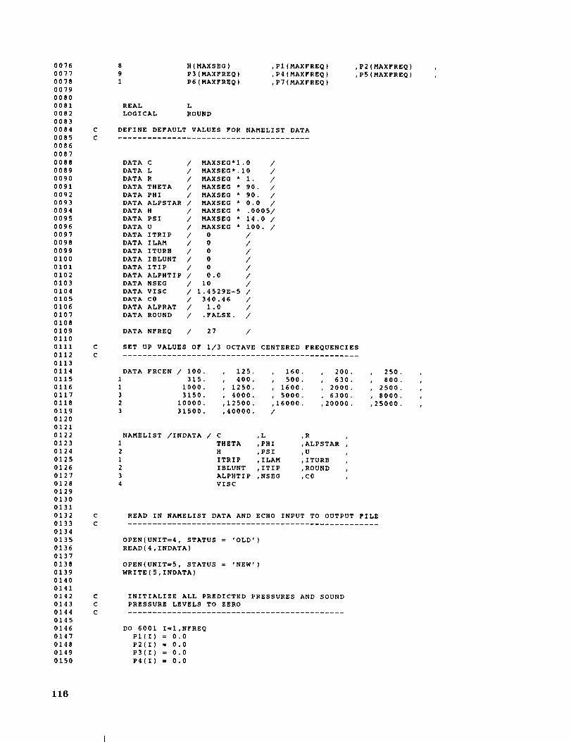
0076
0077
0078
0079
0080
0081
0082
0083
0084
0085
0086
0087
0088
0089
0090
0091
0092
0093
0094
0095
0096
0097
0098
0099
0100
0101
0102
0103
0104
0105
0106
0107
0108
0109
0110
0111
0112
0113
0114
0115
0116
0117
0118
0119
0120
0121
0122
0123
0124
0125
0126
0127
0128
0129
0130
0131
0132
0133
0134
0135
0136
0137
0138
0139
0140
0141
0142
0143
0144
0145
0146
0147
0148
0149
0150
8 H(MAXSEG) ,PI(MAXFREQ)
9 P3(NAXFREQ) ,P4(MAXFREQ)
1 P6(MAXFREQ) ,P7(MAXFREQ)
REAL L
LOGICAL ROUND
DEFINE DEFAULT VALUES FOR NAMELIST DATA
.......................................
,P2(MAXFREQ)
,P5(MAXFREQ)
DATA C / MAXSEG*I.0 /
DATA L / MAXSEG*.I0 /
DATA R / MAXSEG * 1. /
DATA THETA / MAXSEG * 90. /
DATA PHI / MAXSEG * 90. /
DATA ALPSTAR / MAXSEG * 0.0 /
DATA H / MAXSEG * .0005/
DATA PSI / MAXSEG * 14.0 /
DATA U / MAXSEG * 100. /
DATA ITRIP / 0 /
DATA ILAM / 0 /
DATA ITURB / 0 /
DATA IBLUNT / 0 /
DATA ITIP / 0 /
DATA ALPHTIP / 0.0 /
DATA NSEG / i0 /
DATA VISC / 1.4529E-5 /
DATA CO / 340.46 /
DATA ALPRAT / 1.0 /
DATA ROUND / .FALSE. /
DATA NFREQ / 27 /
SET UP VALUES OF 1/3 OCTAVE CENTERED FREQUENCIES
................................................
DATA FRCEN / 100
1 315
1 1000
3 3150
2 10000
3 31500
125. , 160. , 200. , 250. ,
400. , 500. , 630. , 800. ,
1250. , 1600. , 2000. , 2500. ,
4000. , 5000. , 6300. , 8000. ,
12500. ,16000. ,20000. ,25000. ,
40000. /
NAMELIST /INDATA / C ,L
1 THETA ,PHI
2 H ,PSI
1 ITRIP ,ILAM
2 IBLUNT ,ITIP
3 ALPHTIP ,NSEG
4 VISC
R
ALPSTAR
U
ITURB
ROUND
C0
READ IN NAMELIST DATA AND ECHO INPUT TO OUTPUT FILE
...................................................
OPEN(UNIT=4, STATUS = 'OLD')
READ(4,INDATA)
OPEN(UNIT=5, STATUS = 'NEW')
WRITE(5,INDATA)
INITIALIZE ALL PREDICTED PRESSURES AND SOUND
PRESSURE LEVELS TO ZERO
............................................
DO 6001 I=I,NFREQ
PI(I) = 0.0
P2(I) = 0.0
P3(I) = 0.0
P4(I) = 0.0
116

0151
0152
0153
0154
0155
0156
0157
0158
0159
0160
0161
0162
0163
0164
0165
0166
0167
0168
0169
0170
0171
0172
0173
0174
0175
0176
0177
0178
0179
0180
0181
0182
0183
0184
0185
0186
0187
0188
0189
0190
0191
0192
0193
0194
0195
0196
0197
0198
0199
0200
0201
0202
0203
0204
0205
0206
0207
0208
0209
0210
0211
0212
0213
0214
0215
0216
0217
0218
0219
0220
0221
0222
0223
0224
0225
C
C
C
C
C
C
C
C
C
e5(i) = 0.0
P6(i) = 0.0
p7(i) = 0.0
DO 6002 J=1,7
SPL(J,I) = 0.0
6002 CONTINUE
6001 CONTINUE
FOR EACH BLADE SEGMENT, MAKE A NOISE PREDICTION ACCORDING
TO THE MECHANISMS SELECTED. TIP NOISE IS PREDICTED FOR
THE LAST SEGMENT ONLY.
DO 6000 III=I,NSEG
IF (ILAM .EQ. i)
1 CALL LBLVS(ALPSTAR(III),C(III),U(III),FRCEN,SPLLBL,
2 THETA(III),PHI(III),L(III),R(III),NFREQ,
3 VISC,C0)
IF (ITURB .EQ. I}
1 CALL TBLTE(ALPSTAR(III),C(III),U(IIi),FRCEN,ITRIP,SPLP,
1 SPLS,SPLALPH,SPLTBL,THETA(III),PHI(III),L(III),R(III],
2 NFREQ,VISC,C0)
IF (IBLUNT .EQ. 1)
1 CALL BLUNT(ALPSTAR(III),C(III),U(III) ,FRCEN,ITRIP,SPLBLNT,
1 THETA(III),PHI(III),L(III),R(III),H(III),PSI(III),
2 NFREQ,VISC,C0)
IF ((ITIP .EQ. 1) .AND. (III .EQ. NSEG))
1 CALL TIPNOIS(ALPHTIP,ALPRAT,C(III},U(III),FRCEN,SPLTIP,
2 THETA,PHI,R(III),NFREQ,VISC,C0,ROUND)
ADD IN THIS SEGMENT'S CONTRIBUTION ON A MEAN-SQUARE
PRESSURE BASIS
DO 989 I=I,NFREQ
IF (ILAM .EQ. I) THEN
P5(I) = P5(I) + 10.**(SPLLBL(I)/10.)
ENDIF
IF (ITURB .EQ. I) THEN
PI(I) = PI(I) + 10.**(SPLP(I)/10. )
P2(I) = P2(I) + 10.**(SPLS(I)/10. )
P3(I) = P3(I) + 10.**(SPLALPH(I)/10.)
ENDIF
IF (IBLUNT .EQ. 1) THEN
P6(I) = P6(I) + 10.**(SPLBLNT(I)/10.)
ENDIF
IF ((ITIP .EQ. i) .AND. (III .EQ. NSEG)) THEN
P7(I) = P7(I) + 10.**(SPLTIP(I)/10.)
ENDIF
COMPUTE TOTAL PRESSURE FOR THE SEGMENT FOR ALL MECHANISMS
P4(I) = PI(I) + P2(I) + P3(I) + P5(I) + P6(I) + P7(I)
989 CONTINUE
6000 CONTINUE
C CONTRIBUTIONS FROM ALL SEGMENTS ARE NOW ACCOUNTED FOR.
C COMPUTE SOUND PRESSURE LEVELS FOR EACH MECHANISM AND
C FOR THE TOTAL
C
117

0226
0227
0228
0229
0230
0231
0232
0233
0234
0235
0236
0237
0238
0239
0240
0241
0242
0243
0244
0245
0246
0247
0248
0249
0250
0251
0252
0253
0254
0255
0256
0257
0258
0259
0260
0261
0262
0263
0264
0265
DO 6003 I=I,NFREQ
IF (PI(I
IF (P2(I
IF (P3(I
IF (P4(I
IF {P5(I
IF (P6(I
IF (P7{I
6003 CONTINUE
.NE 0
.NE 0
.NE 0
.NE 0
.NE 0
.NE 0
.NE 0
SPL(I,I) = I0 *ALOGIO
SPL(2,I) = I0 *ALOG10
SPL(3,I) = I0 *ALOGIO
SPL(4,I) = i0 *ALOG10
SPL(5,I) = I0 *ALOGI0
SPL(6,I) = I0 *ALOG10
SPL(7,I) = I0 *ALOGI0
Pl(i)
P2(I)
P3(I)
P4(I)
PS(I)
P6(I)
P7(I)
WRITE OUTPUT FILE
WRITE(5,7000)
DO 6005 I=I,NFREQ
WRITE(5,7100) FRCEN(I), (SpL(J,I),J=I,3), (SPL(J,I),J=5,7),
1 SPL(4,I)
IF (MOD(I,5) .EQ. 0) WRITE(5,7200)
6005 CONTINUE
7000 FORMAT(IHI,52X, 'ONE-THIRD OCTAVE',/,50X,'SOUND PRESSURE LEVELS'
1 ////,5x,' ,,, PRESSURE ',
2 ' SUCTION ',' SEPARATION '/,
3 5X,' FREQUENCY(BZ) ', ' SIDE TBL ',
4 ' SIDE TBL ', ' SIDE TBL ',
5 ' LAMINAR ',' BLUNTNESS i'6 ' TIP ',' TOTAL ,
7 /,5X,8( ................ ),/)
7100 FORMAT(8FI5.3)
7200 FORMAT(' ')
8000 FORMAT(I3)
8002 FORMAT(4110)
STOP
END
118

OO01
0002
0003
0004
0005
0006
0007
0008
0009
0010
0011
0012
0013
0014
0015
0016
0017
0018
0019
0020
0021
0022
0023
0024
0025
0026
0027
0028
0029
0030
0031
0032
0033
0034
0035
0036
0037
0038
0039
0040
0041
0042
0043
0044
0045
0046
0047
0048
0049
0050
0051
0052
0053
0054
0055
0056
0057
0058
0059
0060
0061
0062
0063
0064
0065
0066
0067
0068
0069
0070
0071
0072
0073
0074
0075
C
C
C
C
C
C
C
C
C
C
C
C
C
C
C
C
C
C
C
C
C
C
C
C
C
C
C
C
C
C
C
C
C
C
C
C
C
C
C
C
C
C
C
C
C
C
C
SUBROUTINE LBLVS(ALPSTAR,C,U ,FRCEN,SPLLAM,THETA,PHI,L,R,
1 NFREQ,VISC,C0)
PARAMETER (MAXFREQ = 27)
***** VARIABLE DEFINITIONS *****
................................
VARIABLE NAME DEFINITION UNITS
ALPSTAR
C
C0
D
DBARH
DELTAP
DSTRP
DSTRS
E
FRCEN
G1
G2
G3
ITRIP
L
M
NFREQ
OASPL
PHI
R
RC
RC0
SCALE
SPLLAM
STPRIM
STIPRIM
STPKPRM
THETA
U
VISC
ANGLE OF ATTACK DEGREES
CHORD LENGTH METERS
SPEED OF SOUND METERS/SEC
REYNOLDS NUMBER RATIO
HIGH FREQUENCY DIRECTIVITY ---
PRESSURE SIDE BOUNDARY LAYER
THICKNESS METERS
PRESSURE SIDE BOUNDARY LAYER
DISPLACEMENT THICKNESS METERS
SUCTION SIDE BOUNDARY LAYER
DISPLACEMENT THICKNESS METERS
STROUHAL NUMBER RATIO ---
1/3 OCTAVE FREQUENCIES HERTZ
SOUND PRESSURE LEVEL FUNCTION DB
OVERALL SOUND PRESSURE LEVEL
FUNCTION DB
OVERALL SOUND PRESSURE LEVEL
FUNCTION DB
FLAG TO TRIP BOUNDARY LAYER
SPAN METERS
MACH NUMBER
NUMBER OF FREQUENCIES
OVERALL SOUND PRESSURE LEVEL DB
DIRECTIVITY ANGLE DEGREES
OBSERVER DISTANCE FROM SEGMENT METERS
REYNOLDS NUMBER BASED ON CHORD
REFERENCE REYNOLDS NUMBER ---
GEOMETRIC SCALING TERM
SOUND PRESSURE LEVEL DUE TO
LAMINAR MECHANISM DB
STROUHAL NUMBER BASED ON PRESSURE
SIDE BOUNDARY LAYER THICKNESS
REFERENCE STROUHAL NUMBER
PEAK STROUHAL NUMBER
DIRECTIVITY ANGLE
FREESTREAM VELOCITY
KINEMATIC VISCOSITY
DEGREES
METERS/SEC
M2/SEC
DIMENSION STPRIM(MAXFREQ) ,SPLLAM(MAXFREQ)
REAL L ,M
COMPUTE REYNOLDS NUMBER AND MACH NUMBER
.......................................
M = U / CO
RC = U * C/VISC
COMPUTE BOUNDARY LAYER THICKNESSES
..................................
CALL THICK(C,U ,ALPSTAR,ITRIP,DELTAP,DSTRS,DSTRP,C0,VISC)
,FRCEN(MAXFREQ)
COMPUTE DIRECTIVITY FUNCTION
119

0076
0077
0078
0079
0080
0081
0082
0083
0084
0085
0086
0087
0088
0089
0090
0091
0092
0093
0094
0095
0096
0097
0098
0099
0100
0101
0102
0103
0104
0105
0106
0107
0108
0109
0110
0111
0112
0113
0114
0115
0116
0117
0118
0119
0120
0121
0122
0123
0124
0125
0126
0127
0120
0129
0130
0131
0132
0133
0134
0135
0136
0137
0138
0139
0140
0141
0142
0143
0144
0145
0146
CALL DIRECTH(M,THETA,PHI,DBARH)
COMPUTE REFERENCE STROUHAL NUMBER
.................................
IF (RC .LE. 1.3E+05) STIPRIM = .18
IF((RC .GT. 1.3E+05).AND-(RC.LE.4.0E+05))STIPRIM=.001756*RC**.3931
IF (RC .GT. 4.0E+05) STIPRIM = .28
STPKPRM = 10.**(-.04*ALPSTAR) * STIPRIM
COMPUTE REFERENCE REYNOLDS NUMBER
.................................
IF (ALPSTAR .LE. 3.0} RC0=lO.**(.215*ALPSTAR+4.978}
IF (ALPSTAR .GT. 3.0) RC0=10.**(.120*ALPSTAR+5.263}
COMPUTE PEAK SCALED SPECTRUM LEVEL
..................................
D = RC / RC0
IF (D .LE. .3237) G2=77.852*ALOG10(D)+15.328
IF ( (D .GT. .3237).AND. (D .LE. .5689))
1 G2 = 65.188*ALOG10(D) + 9.125
IF ( (D .GT. .5689}.AND. (D .LE. 1.7579) )
1 G2 = -114.052 * ALOG10(D)**2.
IF ((D .GT. 1.7579}.AND. (D .LE. 3.0889))
1 G2 = -65.188*ALOG10(D)+9.125
IF (D .GT. 3.0889) G2 _-77.852*ALOG10(D)+15.328
G3
SCALE
= 171.04 - 3.03 * ALPSTAR
= 10. * ALOGI0(DELTAP*M**5*DBARH*L/R**2)
COMPUTE SCALED SOUND PRESSURE LEVELS FOR EACH STROUHAL NUMBER
.............................................................
DO I00 I=I,NFREQ
STPRIM(I) = FRCEN(I) * DELTAP / U
= STPRIM(I) / STPKPRM
IF (E .LT. .5974) GI=39.8*ALOG10(E)-I1.12
IF ((E .GE. .5974).AND.(E .LE..8545))
G1 = 98.409 * ALOG10(E} + 2.0
IF ((E .GE. .8545).AND. (E .LT. 1.17))
G1 = -5.076+SQRT(2.484-506.25*(ALOG10(E) )*,2.)
IF ((E .GE. 1.17).AND. (E .LT. 1.674))
G1 = -98.409 * ALOG10(E) + 2.0
IF (E .GE. 1.674) G1=-39.80*ALOG10(E)-11.12
SPLLAM(I) = G1 + G2 + G3 + SCALE
I00 CONTINUE
RETURN
END
120

0001
0002
0003
0004
0005
0006
0007
0008
0009
0010
0011
0012
0013
0014
0015
0016
0017
0018
0019
0020
0021
0022
0023
0024
0025
0026
0027
0028
0029
0030
0031
0032
0033
0034
0035
0036
0037
0038
0039
0040
0041
0042
0043
0044
0045
0046
0047
0048
0049
0050
0051
0052
0053
0054
0055
0056
0057
0058
0059
0060
0061
0062
0063
0064
0065
0066
0067
0068
0069
0070
0071
0072
0073
0074
0075
SUBROUTINE TBLTE(ALPSTAR,C,U ,FRCEN,ITRIP,SPLP,SPLS,
1 SPLALPH,SPLTBL,THETA,PHI,L,R,NFREQ,VISC,C0)
***** VARIABLE DEFINITIONS *****
................................
VARIABLE NAME
A
A0
A02
AA
ALPSTAR
AMAXA
AMAXA0
AMAXA02
AMAXB
AMINA
AMINA0
AMINA02
AMINB
ARA0
ARA02
B
B0
BB
BETA
BETA0
BMAXB
BMAXB0
BMINB
BMINB0
BRB0
C
C0
DBARH
DBARL
DELKI
DELTAP
DSTRP
DSTRS
FRCEN
GAMMA
GAMMA0
ITRIP
K1
K2
L
M
NFREQ
PHI
P1
P2
P4
R
RC
RDSTRP
RDSTRS
SPLALPH
SPLP
DEFINITION UNITS
STROUHAL NUMBER RATIO
FUNCTION USED IN 'A' CALCULATION
FUNCTION USED IN 'A' CALCULATION
'A' SPECTRUM SHAPE EVALUATED AT
STROUHAL NUMBER RATIO DB
ANGLE OF ATTACK DEGREES
MAXIMUM 'A' CURVE EVALUATED AT
STROUHAL NUMBER RATIO DB
MAXIMUM 'A' CURVE EVALUATED AT A0 DB
MAXIMUM 'A' CURVE EVALUATED AT A02 DB
MAXIMUM 'A' CURVE EVALUATED AT B DB
MINIMUM 'A' CURVE EVALUATED AT
STROUHAL NUMBER RATIO DB
MINIMUM 'A' CURVE EVALUATED AT A0 DB
MINIMUM 'A' CURVE EVALUATED AT A02 DB
MINIMUM 'A' CURVE EVALUATED AT B DB
INTERPOLATION FACTOR ---
INTERPOLATION FACTOR ---
STROUHAL NUMBER RATIO ---
FUNCTION USED IN 'B' CALCULATION
'B' SPECTRUM SHAPE EVALUATED AT
STROUBAL NUMBER RATIO
USED IN 'B COMPUTATION
USED IN 'B COMPUTATION
MAXIMUM 'B EVALUATED AT B
MAXIMUM 'B EVALUATED AT B0
MINIMUM 'B EVALUATED AT B
MINIMUM 'B EVALUATED AT B0
INTERPOLATION FACTOR
CHORD LENGTH
SPEED OF SOUND
HIGH FREQUENCY DIRECTIVITY
LOW FREQUENCY DIRECTIVITY
CORRECTION TO AMPLITUDE FUNCTION
PRESSURE SIDE BOUNDARY LAYER THICKNESS METERS
PRESSURE SIDE DISPLACEMENT THICKNESS METERS
SUCTION SIDE DISPLACEMENT THICKNESS METERS
ARRAY OF CENTERED FREQUENCIES HERTZ
USED IN 'B' COMPUTATION ---
USED IN 'B' COMPUTATION ---
TRIGGER TO TRIP BOUNDARY LAYER
AMPLITUDE FUNCTION DB
AMPLITUDE FUNCTION DB
SPAN METERS
MACH NUMBER ---
NUMBER OF CENTERED FREQUENCIES ---
DIRECTIVITY ANGLE DEGREES
PRESSURE SIDE PRESSURE NT/M2
SUCTION SIDE PRESSURE NT/M2
PRESSURE FROM ANGLE OF ATTACK
CONTRIBUTION NT/M2
SOURCE TO OBSERVER DISTANCE METERS
REYNOLDS NUMBER BASED ON CHORD ---
REYNOLDS NUMBER BASED ON PRESSURE
SIDE DISPLACEMENT THICKNESS ---
REYNOLDS NUMBER BASED ON SUCTION
SIDE DISPLACEMENT THICKNESS
SOUND PRESSURE LEVEL DUE TO ANGLE OF
ATTACK CONTRIBUTION DB
SOUND PRESSURE LEVEL DUE TO PRESSURE
SIDE OF AIRFOIL DB
DB
DB
DB
DB
DB
DB
METERS
METERS/SEC
DB
121

0076
0077
0078
0079
0080
0081
0082
0083
0084
0085
0086
0087
0088
0089
0090
0091
0092
0093
0094
0095
0096
0097
0098
0099
0100
0101
0102
0103
0104
0105
0106
0107
0108
0109
0110
0111
0112
0113
0114
0115
0116
0117
0118
0119
0120
0121
0122
0123
0124
0125
0126
0127
0128
0129
0130
0131
0132
0133
0134
0135
0136
0137
0138
0139
0140
0141
0142
0143
0144
0145
0146
0147
0148
0149
0150
SPLS
SPLTBL
STP
STS
ST1
STIPRIM
ST2
STPEAK
SWITCH
THETA
U
VISC
XCHECK
SOUND PRESSURE LEVEL DUE TO SUCTION
SIDE OF AIRFOIL
TOTAL SOUND PRESSURE LEVEL DUE TO
TBLTE MECHANISM
PRESSURE SIDE STROUHAL NUMBER
SUCTION SIDE STROUHAL NUMBER
PEAK STROUHAL NUMBER
PEAK STROUHAL NUMBER
PEAK STROUHAL NUMBER
PEAK STROUHAL NUMBER
LOGICAL FOR COMPUTATION OF ANGLE
OF ATTACK CONTRIBUTION
DIRECTIVITY ANGLE
VELOCITY
KINEMATIC VISCOSITY
USED TO CHECK FOR ANGLE OF ATTACK
CONTRIBUTION
PARAMETER (MAXFREQ = 27)
DIMENSION SPLTBL(MAXFREQ) ,SPLP(MAXFREQ)
I SPLALPH(MAXFREQ) ,STP(MAXFREQ)
1 STS(MAXFREQ) ,FRCEN(MAXFREQ)
LOGICAL SWITCH
REAL L,M,KI,K2
RC = U * C / VISC
M = U / C0
,SPLS(MAXFREQ)
COMPUTE BOUNDARY LAYER THICKNESSES
..................................
CALL THICK(C,U ,ALPSTAR,ITRIP,DELTAP,DSTRS,DSTRP,C0,VISC)
COMPUTE DIRECTIVITY FUNCTION
............................
CALL DIRECTL(M,THETA,PHI,DBARL)
CALL DIRECTH(M,THETA,PHI,DBARH)
CALCULATE THE REYNOLDS NUMBERS BASED ON PRESSURE AND
SUCTION DISPLACEMENT THICKNESS
...................................................
RDSTRS = DSTRS * U / VISC
RDSTRP = DSTRP * U / VISC
DETERMINE PEAK STROUHAL NUMBERS TO BE USED FOR
'A' AND 'B' CURVE CALCULATIONS
..............................................
ST1 = .02 * M ** (-.6)
IF (ALPSTAR .LE. 1.333) ST2 = ST1
IF ((ALPSTAR .GT. 1.333).AND. (ALPSTAR .LE. 12.5))
1 ST2 = STI*I0.**(.0054*(ALPSTAR-I.333)**2. )
IF (ALPSTAR .GT. 12.5) ST2 = 4.72 * ST1
STIPRIM = (STI+ST2)/2.
CALL AOCOMP(RC,A0)
CALL AOCOMP(3.*RC,A02)
EVALUATE MINIMUM AND MAXIMUM 'A' CURVES AT A0
..............................................
CALL AMIN(A0,AMINA0)
CALL AMAX(A0,AMAXA0)
DB
DB
DEGREES
METERS/SEC
M2/SEC
122

0151
0152
0153
0154
0155
0156
0157
0158
0159
0160
0161
0162
0163
0164
0165
0166
0167
0168
0169
0170
0171
0172
0173
0174
0175
0176
0177
0178
0179
0180
0181
0182
0183
0184
0185
0186
0187
0188
0189
0190
0191
0192
0193
0194
0195
0196
0197
0198
0199
0200
0201
0202
0203
0204
O2O5
0206
0207
0208
0209
0210
0211
0212
0213
0214
0215
0216
0217
0218
0219
0220
0221
0222
0223
0224
0225
CALL AMIN(A02,AMINA02)
CALL AMAX(A02,AMAXA02)
COMPUTE 'A' MAX/MIN RATIO
.........................
ARA0 = (20. + AMINA0) / (AMINA0 - AMAXA0)
ARA02 = (20. + AMINA02)/ (AMINA02- AMAXA02)
COMPUTE B0 TO BE USED IN 'B' CURVE CALCULATIONS
...............................................
IF (RC .LT. 9.52E+04) B0 = .30
IF ((RC .GE. 9.52E+04).AND.(RC .LT. 8.57E+05))
1 B0 = (-4.48E-13)*(RC-8.57E+05)**2. + .56
IF (RC .GE. 8.57E+05) B0 = .56
EVALUATE MINIMUM AND MAXIMUM 'B' CURVES AT B0
..............................................
CALL BMIN(B0,BMINB0)
CALL BMAX(B0,BMAXB0)
COMPUTE 'B' MAX/MIN RATIO
.........................
BRB0 = (20. + BMINB0) / (BMINB0 - BMAXB0)
FOR EACH CENTER FREQUENCY, COMPUTE AN
'A' PREDICTION FOR THE PRESSURE SIDE
.....................................
STPEAK = ST1
DO i00 I=I,NFREQ
STP(I) = FRCEN(I) * DSTRP / U
A = ALOGI0(STP(I) / STPEAK )
CALL AMIN(A,AMINA}
CALL AMAX(A,AMAXA)
AA = AMINA + ARA0 * (AMAXA - AMINA)
IF (RC .LT. 2.47E+05) K1 = -4.31 * ALOGI0(RC) + 156.3
IF((RC .GE. 2.47E+O5).AND. (RC .LT. 8.0E+05))
K1 = -9.0 * ALOGI0(RC) + 181.6
IF (RC .GT. 8.0E+05) K1 = 128.5
IF (RDSTRP .LE. 5000.) DELKI = -ALPSTAR*(5.29-1.43*
ALOGI0(RDSTRP) )
IF (RDSTRP .GT. 5000.) DELKI = 0.0
SPLP(I)=AA+KI-3.+I0.*ALOGI0(DSTRP*M**5.*DBARH*L/R**2. )+DELKI
GAMMA = 27.094 * M + 3.31
BETA = 72.650 * M + 10.74
GAMMA0 = 23.430 * M + 4.651
BETA0 =-34.190 * M - 13.820
IF (ALPSTAR .LE. (GAMMA0-GAMMA)) K2 = -i000.0
IF ((ALPSTAR.GT.(GAMMA0-GAMMA)).AND.(ALPSTAR.LE.(GAMMA0+GAMMA)))
1 K2=SQRT(BETA**2.-(BETA/GAMMA)**2.*(ALPSTAR-GAMMA0)**2.)+BETA0
IF (ALPSTAR .GT. (GAMMA0+GAMMA)) K2 = -12.0
K2 = K2 + K1
STS(I) = FRCEN(I) * DSTRS / U
CHECK FOR 'A' COMPUTATION FOR SUCTION SIDE
..........................................
123
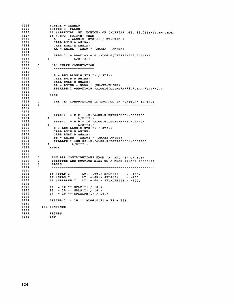
0226
0227
0228
0229
0230
0231
0232
0233
0234
0235
0236
0237
0238
0239
0240
0241
0242
0243
0244
0245
0246
0247
0248
0249
0250
0251
0252
0253
0254
0255
0256
0257
0258
0259
0260
0261
0262
0263
0264
0265
0266
0267
0268
0269
0270
0271
0272
0273
0274
0275
0276
0277
0278
0279
0280
0281
0282
0283
0284
XCHECK = GAMMA0
SWITCH = .FALSE.
IF ( (ALPSTAR .GE. XCHECK).OR.(ALPSTAR .GT. 12.5))SWITCH=.TRUE.
IF (.NOT. SWITCH) THEN
A = ALOG10(STS(I) / STIPRIM )
CALL AMIN(A,AMINA)
CALL AMAX(A,AMAXA)
AA = AMINA + ARA0 * (AMAXA - AMINA)
SPLS(I} = AA+K1-3.+10.*ALOG10(DSTRS*M**5.*DBARH*
L/R**2.)
'B' CURVE COMPUTATION
S = ABS(ALOGI0(STS(I) / ST2))
CALL BMIN(B,BMINB)
CALL BMAX(B,BMAXB)
BB = BMINB + BRB0 * (BMAXB-BMINB)
SPLALPH(I)=BB+K2+I0.*ALOGI0(DSTRS*M**5.*DBARH*L/R**2.)
ELSE
THE 'A' COMPUTATION IS DROPPED IF 'SWITCH' IS TRUE
..................................................
SPLS(I) = 0.0 + 10.*ALOGI0(DSTRS*M**5.*DBARL*
1 L/R**2.)
SPLP(I) = 0.0 + 10.*ALOGI0(DSTRS*M**5.*DBARL*
1 L/R**2.)
B = ABS(ALOG10(STS(I) / ST2))
CALL AMIN(B,AMINB)
CALL AMAX(B,AMAXB)
EB = AMINB + ARA02 * (AMAXB-AMINB)
SPLALPH(I)=BB+K2+10.*ALOGI0(DSTRS*M**5.*DBARL*
1 L/R**2.)
ENDIF
SUM ALL CONTRIBUTIONS FROM 'A' AND 'B' ON BOTH
PRESSURE AND SUCTION SIDE ON A MEAN-SQUARE PRESSURE
BASIS
...................................................
IF (SPLP(I} .LT. -I00.) SPLP(I) = -100.
IF (SPLS(I) .LT. -i00.) SPLS(I) = -100.
IF (SPLALPH(I) .LT. -i00.) SPLALPH(I) = -i00.
P1 = 10.**(SPLP(I) / 10.)
P2 = 10.**(SPLS(I) / 10.)
P4 = 10.**(SPLALPH(I) / 10.)
SPLTBL(I) = 10. * ALOG10(P1 + P2 + P4)
100 CONTINUE
RETURN
END
124

0001
0002
0003
0004
0005
0006
0007
0008
0009
0010
0011
0012
0013
0014
SUBROUTINE AMIN(A,AMINA)
THIS SUBROUTINE DEFINES THE CURVE FIT CORRESPONDING
TO THE A-CURVE FOR THE MINIMUM ALLOWED REYNOLDS NUMBER.
Xl = ASS(A)
IF (Xl
IF((Xl
IF (Xl
.LE. .204) AMINA=SQRT(67.552-886.788*X1**2.)-8.219
.GT. .204).AND. (Xl .LE. .244))AMINA=-32.665*XI+3.981
.GT. .244)AMINA=-I42.795*XI**3.+I03.656*X1**2.-57.757*XI+6.006
RETURN
END
0001
0002
0003
0004
0005
0006
0007
0008
0009
0010
0011
0012
0013
SUBROUTINE AMAX(A,AMAXA)
THIS SUBROUTINE DEFINES THE CURVE FIT CORRESPONDING
TO THE A-CURVE FOR THE MAXIMUM ALLOWED REYNOLDS NUMBER.
Xl = ABS(A)
IF (Xl .LE. .13)AMAXA=SQRT(67.552-886.788*XI**2. )-8.219
IF( (Xl .GT. .13).AND. (Xl .LE. .321))AMAXA=-I5.901*XI+I.098
IF (Xl .GT. .321)AMAXA=-4.669*XI**3.+3.491*XI**2.-16.699*XI+I.149
RETURN
END
0001
0002
0003
0004
0005
0006
0007
0008
0009
0010
0011
0012
0013
SUBROUTINE BMIN(B,BMINB)
THIS SUBROUTINE DEFINES THE CURVE FIT CORRESPONDING
TO THE B-CURVE FOR THE MINIMUM ALLOWED REYNOLDS NUMBER.
Xl = ASS(B)
IF (Xl .LE. .13)BMINB=SQRT(16.888-886.788*XI**2. )-4.109
IF((X1 .GT. .13).AND. (XI .LE. .145))BMINB=-83.607*XI+8.138
IF (X1.GT..145)BMINB=-817.81*XI**3.+355.21*XI**2.-135.024*XI+IO.619
RETURN
END
0001
0002
0003
0004
0005
0006
0007
0008
0009
0010
0011
0012
0013
SUBROUTINE BMAX(B,BMAXB)
THIS SUBROUTINE DEFINES THE CURVE FIT CORRESPONDING
TO THE B-CURVE FOR THE MAXIMUM ALLOWED REYNOLDS NUMBER.
X1 = ASS(B)
IF (Xl .LE. .i) BMAXB=SQRT(16.888-886.788*XI**2.)-4.109
IF((XI .GT..1).AND.(XI .LE..187))BMAXB=-31.313*Xl+I.854
IF (XI.GT..187)BMAXH=-80.541*XI**3.+44.174*XI**2.-39.381*XI+2.344
RETURN
END
125

OO01
0002
0003
0004
OO05
0006
0007
0008
0009
0010
0011
SUBROUTINE AOCOMP(RC,A0)
THIS SUBROUTINE DETERMINES WHERE THE A-CURVE
TAKES ON A VALUE OF -20 dB.
IF (RC .LT. 9.52E+04) A0 = .57
IF ( (RC .GE. 9.52E+04).AND. (RC .LT. 8.57E+05))
1 A0 = (-9.57E-13)*(RC-8.57E+05)**2. + 1.13
IF (RC .GE. 8.57E+05) A0 = 1.13
RETURN
END
0001
0002
0003
0004
0005
0006
0007
0008
0009
0010
0011
0012
0013
0014
0015
0016
0017
SUBROUTINE DIRECTH(M,THETA,PHI,DBAR)
THIS SUBROUTINE COMPUTES THE HIGH FREQUENCY
DIRECTIVITY FUNCTION FOR THE INPUT OBSERVER LOCATION
REAL M,MC
DEGRAD = .017453
MC = .8 * M
THETAR = THETA * DEGRAD
PHIR = PHI * DEGRAD
DBAR=2.*SIN(THETAR/2.)**2.*SIN(PHIR)**2./((I.+M*COS(THETAR))*
1 (I.+(M-MC)*COS(THETAR))*'2.)
RETURN
END
0001
0002
0003
0004
0005
0006
0007
0008
0009
0010
0011
0012
0013
0014
0015
0016
0017
SUBROUTINE DIRECTL(M,THETA,PHI,DBAR)
THIS SUBROUTINE COMPUTES THE LOW FREQUENCY
DIRECTIVITY FUNCTION FOR THE INPUT OBSERVER LOCATION
REAL M,MC
DEGRAD = .017453
MC = .8 * M
THETAR = THETA * DEGRAD
PHIR = PHI * DEGRAD
DBAR = (SIN(THETAR)*SIN(PHIR))**2/(1.+M*COS(THETAR))**4
RETURN
END
126

0001
0002
0003
0004
OOO5
0006
0007
0008
0009
0010
0011
0012
0013
0014
0015
0016
0017
0018
0019
0020
0021
0022
0023
0024
0025
0026
0027
0028
0029
0030
0031
0032
0033
0034
0035
0036
0037
0038
0039
0040
0041
0042
0043
0044
0045
0046
0047
0048
0049
0050
0051
0052
0053
0054
0055
0056
0057
0058
0059
0060
0061
0062
0063
0064
0065
0066
0067
0068
0069
0070
0071
0072
0073
0074
0075
C
C
C
C
C
C
C
C
C
C
C
C
C
C
C
C
C
C
C
C
C
C
C
C
C
C
C
C
C
C
C
C
C
C
C
C
C
C
C
C
C
C
C
C
C
C
C
C
C
C
C
SUBROUTINE BLUNT(ALPSTAR,C,U ,FRCEN,ITRIP,SPLBLNT,THETA,PHI,
1 L,R,H,PSI,NFREQ,VISC,C0)
***** VARIABLE DEFINITIONS *****
................................
VARIABLE NAME DEFINITION UNITS
ALPSTAR
ATERM
C
C0
DBARH
DELTAP
DSTARH
DSTRAVG
DSTRP
DSTRS
ETA
FRCEN
F4TEMP
G4
G5
G50
G514
H
HDSTAR
HDSTARL
HDSTARP
ITRIP
L
M
NFREQ
PHI
PSI
R
RC
SCALE
SPLBLNT
STPEAK
STPPP
THETA
U
VISC
ANGLE OF ATTACK
USED TO COMPUTE PEAK STROUHAL NO.
CHORD LENGTH
SPEED OF SOUND
HIGH FREQUENCY DIRECTIVITY
PRESSURE SIDE BOUNDARY LAYER
THICKNESS METERS
AVERAGE DISPLACEMENT THICKNESS
OVER TRAILING EDGE BLUNTNESS
AVERAGE DISPLACEMENT THICKNESS METERS
PRESSURE SIDE DISPLACEMENT THICKNESS METERS
SUCTION SIDE DISPLACEMENT THICKNESS METERS
RATIO OF STROUHAL NUMBERS
ARRAY OF 1/3 OCTAVE CENTERED FREQ. HERTZ
G5 EVALUATED AT MINIMUM HDSTARP DB
SCALED SPECTRUM LEVEL DB
SPECTRUM SHAPE FUNCTION DB
G5 EVALUATED AT PSI=0.0 DB
G5 EVALUATED AT PSI=f4.0 DB
TRAILING EDGE BLUNTNESS METERS
BLUNTNESS OVER AVERAGE DISPLACEMENT
THICKNESS ---
MINIMUM ALLOWED VALUE OF HDSTAR
MODIFIED VALUE OF HDSTAR
TRIGGER FOR BOUNDARY LAYER TRIPPING
SPAN
MACH NUMBER
NUMBER OF CENTERED FREQUENCIES
DIRECTIVITY ANGLE DEGREES
TRAILING EDGE ANGLE DEGREES
SOURCE TO OBSERVER DISTANCE METERS
REYNOLDS NUMBER BASED ON CHORD ---
SCALING FACTOR
SOUND PRESSURE LEVELS DUE TO
BLUNTNESS DB
PEAK STROUHAL NUMBER
STROUHAL NUMBER
DIRECTIVITY ANGLE
FREESTREAM VELOCITY
KINEMATIC VISCOSITY
DEGREES
METERS
METERS/SEC
METERS
METERS/SEC
M2/SEC
PARAMETER (MAXFREQ = 27)
DIMENSION SPLBLNT(MAXFREQ) ,FRCEN(MAXFREQ)
REAL M,L
COMPUTE NECESSARY QUANTITIES
............................
,STPPP(MAXFREQ)
M = U /CO
RC = U * C / VISC
COMPUTE BOUNDARY LAYER THICKNESSES
..................................
CALL THICK(C,U ,ALPSTAR,ITRIP,DELTAP,DSTRS,DSTRP,C0,VISC)
COMPUTE AVERAGE DISPLACEMENT THICKNESS
DSTRAVG = (DSTRS + DSTRP) / 2.
127

0076
0077
0078
0079
0080
0081
0082
0083
0084
0085
0086
0087
0088
0089
0090
0091
0092
0093
0094
0095
0096
0097
0098
0099
0100
0101
0102
0103
0104
0105
0106
0107
0108
0109
0110
0111
0112
0113
0114
0115
0116
0117
0118
0119
0120
0121
0122
0123
0124
0125
0126
0127
0128
0129
0130
0131
0132
0133
0134
HDSTAR = H / DSTRAVG
DSTARH = i. /HDSTAR
COMPUTE DIRECTIVITY FUNCTION
............................
CALL DIRECTH(M,THETA,PHI,DBARH)
COMPUTE PEAK STROUHAL NUMBER
............................
ATERM = .212 - .0045 * PSI
IF (HDSTAR .GE..2)
1 STPEAK = ATERM / (1.+.235*DSTARH-.0132*DSTARH**2.)
IF (HDSTAR .LT. .2)
1 STPEAK = .1 * HDSTAR + .095 - .00_43 * PSI
COMPUTE SCALED SPECTRUM LEVEL
.............................
IF (HDSTAR .LE. 5.) G4=17.5*ALOG10(HDSTAR)+157.5-1.114*PSI
IF (HDSTAR .GT. 5.) G4=169.7 - 1.114 * PSI
FOR EACH FREQUENCY, COMPUTE SPECTRUM SHAPE REFERENCED TO 0 DB
.............................................................
DO 1000 I=I,NFREQ
STPPP(I) = FRCEN(I) * H / U
ETA = ALOGI0(STPPP(I)/STPEAK)
HDSTARL = HDSTAR
CALL G5COMP(HDSTARL,ETA,G514)
HDSTARP = 6.724 * HDSTAR **2.-4.019*HDSTAR+I.107
CALL G5COMP(HDSTARP,ETA,G50")
G5 = G50 + .0714 * PSI * (G514-G50)
IF (G5 .GT. 0.) G5 = 0.
CALL G5COMP(.25,ETA,F4TEMP)
IF (G5 .GT. F4TEMP) G5 = F4TEMP
SCALE = i0. * ALOGI0(M**5.5*H*DBARH*L/R**2.)
SPLBLNT(I) = G4 + G5 + SCALE
1000 CONTINUE
RETURN
END
128

0001
0002
0003
0004
0OO5
0006
0007
0008
0009
0010
0011
0012
0013
0014
0015
0016
0017
0018
0019
0020
0021
0022
0023
0024
0025
0026
0027
0028
0029
0030
0031
0032
0033
0034
0035
0036
SUBROUTINE G5COMP(HDSTAR,ETA,G5)
REAL M,K,MU
IF (BDSTAR .LT. .25) MU = .1211
IF ((HDSTAR .GT. .25).AND.(HDSTAR .LE. .62))
1 MU=-.2175*HDSTAR + .1755
IF ((HDSTAR .GT. .62).AND.(HDSTAR .LT. 1.15))
1MU = -.0308 * HDSTAR + .0596
IF (HDSTAR .GE. 1.15)MU = .0242
IF (HDSTAR .LE. .02) M = 0.0
IF ((HDSTAR .GE. .02).AND. (HDSTAR .LT. .5) )
I M=68.724*BDSTAR - 1.35
IF ((HDSTAR .GT. .5).AND. (HDSTAR .LE. .62))
1 M = 308.475 * HDSTAR - 121.23
IF ((HDSTAR .GT. .62).AND.(HDSTAR .LE. 1.15))
1 M = 224.811 * HDSTAR - 69.354
IF ((HDSTAR .GT. 1.15) .AND. (HDSTAR .LT. 1.2))
1 M = 1583.28 * HDSTAR - 1631.592
IF (HDSTAR .GT. 1.2} M = 268.344
IF (M .LT. 0.0) M = 0.0
ETA0 = -SQRT((M*M*MU**4)/(6.25+M*M*MU*MU))
K = 2.5*SQRT(I.-(ETA0/MU)**2.)-2.5-M*ETA0
IF (ETA .LE. ETA0) G5 = M * ETA + K
IF ((ETA .GT. ETA0).AND. (ETA .LE. 0. ))G5=2.5*SQRT(1.-(ETA/MU)**2.)-2.5
IF((ETA.GT.0. ).AND. (ETA.LE..03616))G5=SQRT(1.5625-1194.99*ETA**2.)-1.25
IF (ETA .GT. .03616) G5=-155.543 * ETA + 4.375
RETURN
END
129

OO01
0002
0003
0004
0005
0006
0007
0008
0009
0010
0011
0012
0013
0014
0015
0016
0017
0018
0019
0020
0021
0022
0023
0024
0025
0026
0027
0028
0029
0030
0031
0032
0033
0034
0035
0036
0037
0038
0039
0040
0041
0042
0043
0044
0045
0046
0047
0048
0049
0050
0051
0052
0053
0054
0055
0056
0057
0058
0059
0060
0061
0062
0063
0064
0065
0066
0067
0068
0069
0070
0071
0072
0073
0074
SUBROUTINE TIPNOIS(ALPHTIP,ALPRAT,C,U ,FRCEN,SPLTIP,THETA,PHI,
R,NFREQ,VISC,C0,ROUND)
................................
***** VARIABLE DEFINITIONS *****
................................
VARIABLE NAME DEFINITION
.......................
ALPHTIP TIP ANGLE OF ATTACK
ALPRAT TIP LIFT CURVE SLOPE
ALPTIPP CORRECTED TIP ANGLE OF ATTACK
C CHORD LENGTH
C0 SPEED OF SOUND
DBARH DIRECTIVITY
FRCEN CENTERED FREQUENCIES
L CHARACTERISTIC LENGTH FOR TIP
M MACH NUMBER
MM MAXIMUM MACH NUMBER
NFREQ NUMBER OF CENTERED FREQUENCIES
PHI DIRECTIVITY ANGLE
R SOURCE TO OBSERVER DISTANCE
ROUND LOGICAL SET TRUE IF TIP IS ROUNDED
SCALE SCALING TERM
SPLTIP SOUND PRESSURE LEVEL DUE TO TIP
MECHANISM DB
STPP STROUHAL NUMBER
TERM SCALING TERM
THETA DIRECTIVITY ANGLE
U FREESTREAM VELOCITY
UM MAXIMUM VELOCITY
VISC KINEMATIC VISCOSITY
PARAMETER (MAXFREQ =27)
DIMENSION SPLTIP(MAXFREQ},FRCEN(MAXFREQ)
REAL L,M,MM
LOGICAL ROUND
UNITS
DEGREES
DEGREES
METERS
METERS/SEC
HERTZ
METERS
DEGREES
METERS
DEGREES
METERS/SEC
METERS/SEC
M2/SEC
ALPTIPP = ALPHTIP * ALPRAT
M = U / CO
CALL DIRECTH(M,THETA,PHI,DBARH)
IF (ROUND) THEN
L = .008 * ALPTIPP * C
ELSE
IF (ABS(ALPTIPP) .LE. 2.) THEN
L = (.023 + .0169*ALPTIPP) * C
ELSE
L = (.0378 + .0095*ALPTIPP) * C
ENDIF
ENDIF
MM = (i. + .036*ALPTIPP) * M
UM = MM * CO
TERM = M*M*MM**3.*L**2.*DBARH/R**2.
IF (TERM .NE. 0.0) THEN
SCALE = 10.*ALOGI0(TERM)
ELSE
SCALE = 0.0
ENDIF
DO 100 I=I,NFREQ
STPP = FRCEN(I) * L / UM
SPLTIP(I) = 126.-30.5*(ALOGI0(STPP)+.3)**2. + SCALE
I00 CONTINUE
RETURN
END
130

0001
0002
0003
0004
0005
0006
0007
0008
OO09
0010
0011
0012
0013
0014
0015
0016
0017
0018
0019
0020
0021
0022
0023
0024
0025
0026
0027
0028
0029
0030
0031
0032
0033
0034
0035
0036
0037
0038
0039
0040
0041
0042
0043
0044
0045
0046
0047
0048
00490050
005_
0052
0053
0054
0055
0056
0057
0058
0059
0060
0061
0062
0063
0064
0065
0066
0067
0068
0069
0070
0071
0072
0073
0074
0075
SUBROUTINE THICK(C,U ,ALPSTAR,ITRIP,DELTAP,DSTRS,DSTRP,C0,VISC)
ALPSTAR
C
C0
DELTA0
DELTAP
DSTR0
DSTRP
DSTRS
ITRIP
M
RC
U
VISC
UNITS
ANGLE OF ATTACK
CHORD LENGTH
SPEED OF SOUND
BOUNDARY LAYER THICKNESS AT
ZERO ANGLE OF ATTACK
PRESSURE SIDE BOUNDARY LAYER
THICKNESS
DISPLACEMENT THICKNESS AT ZERO
ANGLE OF ATTACK
PRESSURE SIDE DISPLACEMENT
THICKNESS
SUCTION SIDE DISPLACEMENT
THICKNESS
TRIGGER FOR BOUNDARY LAYER TRIPPING
MACH NUMBER
REYNOLDS NUMBER BASED ON CHORD
FREESTREAM VELOCITY
KINEMATIC VISCOSITY
DEGREES
METERS
METERS/SEC
METERS
METERS
METERS
METERS
METERS
METERS/SEC
M2/SEC
COMPUTE ZERO ANGLE OF ATTACK BOUNDARY LAYER
THICKNESS (METERS) AND REYNOLDS NUMBER
M = U / CO
RC = U * C/VISC
DELTA0 = 10.**(I.6569-.9045*ALOGI0(RC)+
1 .0596*ALOGI0(RC)**2.)*C
IF (ITRIP .EQ. 2) DELTA0 = .6 * DELTA0
COMPUTE PRESSURE SIDE BOUNDARY LAYER THICKNESS
..............................................
DELTAP = 10.**(-.04175*ALPSTAR+.00106*ALPSTAR**2. )*DELTA0
COMPUTE ZERO ANGLE OF ATTACK DISPLACEMENT THICKNESS
IF ((ITRIP .EQ. I) .OR. (ITRIP .EQ. 2)) THEN
IF (RC .LE. .3E+06) DSTR0 = .0601 * RC **(-.114)*C
IF (RC .GT. .3E+06)
i DSTR0=10.**(3.411--1.5397*ALOG10(RC)+.1059*ALOG10(RC)**2.)*C
IF (ITRIP .EQ. 2) DSTR0 = DSTR0 * .6
ELSE
DSTR0=10.**(3.0187-1.5397*ALOG10(RC)+.1059*ALOG10(RC)**2.)*C
ENDIF
PRESSURE SIDE DISPLACEMENT THICKNESS
....................................
DSTRP = 10.**(-.0432*ALPSTAR+.00113*ALPSTAR**2. )*DSTR0
IF (ITRIP .EQ. 3) DSTRP = DSTRP * 1.48
SUCTION SIDE DISPLACEMENT THICKNESS
...................................
IF (ITRIP .EQ. I) THEN
IF (ALPSTAR .LE. 5.) DSTRS=I0.**(.0679*ALPSTAR)*DSTR0
IF( (ALPSTAR .GT. 5.) .AND. (ALPSTAR .LE. 12.5))
1 DSTRS = .381'i0.**( .1516*ALPSTAR)*DSTR0
IF (ALPSTAR .GT. 12.5)DSTRS=I4.296*I0.**( .0258*ALPSTAR)*DSTR0
ELSE
131

0076
0077
0078
0079
0080
0081
0082
0083
IF (ALPSTAR .LE. 7.5)DSTRS =10.**(.0679*ALPSTAR)*DSTR0
IF((ALPSTAR .GT. 7.5).AND. (ALPSTAR .LE. 12.5) )
1 DSTRS = .0162*I0.**(.3066*ALPSTAR)*DSTR0
IF (ALPSTAR .GT. 12.5) DSTRS = 52.42"10.**( .0258*ALPSTAR)*DSTR0
ENDIF
RETURN
END
132
References1. Brooks, Thomas F.; and Schlinker, Robert H.: Progress
in Rotor Broadband Noise Research. Vertica, vol. 7, no. 4,
1983, pp. 287 307.
2. Brooks, T. F.; and Hodgson, T. H.: Trailing Edge Noise
Prediction From Measured Surface Pressures. J. Sound 64
Vibration, vol. 78, no. 1, Sept. 8, 1981, pp. 69 117.
3. Schlinker, Robert H.; and Amiet, Roy K.: Helicopter
Rotor Trailing Edge Noise. NASA CR-3470, 1981. (See
also AIAA Paper 81-2001.)
4. Liu, N. S.; and Shamroth, S. J.: On the Application of
a Hairpin Vortex Model of Wall Turbulence to Trailing
Edge Noise Prediction. NASA CR-177938, 1985.
5. Ffowcs Williams, J. E.; and Hall, L. H.: Aerodynamic
Sound Generation by Turbulent Flow in the Vicinity of
a Scattering Half Plane. J. Fluid Mech., vol. 40, pt. 4,
Mar. 1970, pp. 657-670.
6. Brooks, Thomas F.; and Marcolini, Michael A.: Scaling
of Airfoil Self-Noise Using Measured Flow Parameters.
AIAA J., vol. 23, no. 2, Feb. 1985, pp. 207-213.
7. Chou, S.-T.; and George, A. R.: Effect of Angle of Attack
on Rotor Trailing-Edge Noise. AIAA J., vol. 22, no. 12,
Dec. 1984, pp. 1821 1823.
8. George, Albert R.; and Chou, Shau-Tak: Broadband Rotor
Noise Analyses. NASA CR-3797, 1984.
9. Grosveld, Ferdinand W.: Prediction of Broadband Noise
From Horizontal Axis Wind Turbines. AIAA J. Propuls.
64 Power, vol. 1, no. 4, July Aug. 1985, pp. 292 299.
10. Glegg, S. A. L.; Baxter, S. M.; and Glendinning, A. G.:
The Prediction of Broadband Noise From Wind Turbines.
J. Sound 64 Vibration, vol. 118, no. 2, Oct. 22, 1987,
pp. 217 239.
11. Fink, M. R.; and Bailey, D. A.: Airframe Noise Reduction
Studies and Clean-Airframe Noise Investigation. NASA
CR-159311, 1980.
12. Paterson, Robert W.; Amiet, Roy K.; and Munch, C.
Lee: Isolated Airfoil-Tip Vortex Interaction Noise. AIAA
Paper No. 74-194, Jan. Feb. 1974.
13. Tam, Christopher K. W.: Discrete Tones of Isolated Air-
foils. J. Acoust. Soc. America, vol. 55, no. 6, June 1974,
pp. 1173 1177.
14. Wright, S. E.: The Acoustic Spectrum of Axial Flow
Machines. J. Sound 64 Vibration, vol. 45, no. 2, Mar. 22,
1976, pp. 165 223.
15. Fink, M. R.: Fine Structure of Airfoil Tone Frequency•
UTRC78-10, United Technologies Research Center,Jan. 1978.
16. Paterson, Robert W.; Vogt, Paul G.; Fink, Martin R.;
and Munch, C. Lee: Vortex Noise of Isolated Airfoils. J.
Aircr., vot. 10, no. 5, May 1973, pp. 296 302.
17. George, A. R.; Najjar, F. E.; and Kim, Y. N.: Noise
Due to Tip Vortex Formation on Lifting Rotors.
AIAA-80-1010, June 1980.
18. Brooks, Thomas F.; and Marcolini, Michael A.: Airfoil
Tip Vortex Formation Noise. AIAA J., vol. 24, no. 2,
Feb. 1986, pp. 246 252.
19. Blake, William K.: Aero-Hydroacoustics for Ships, Vol-
ume H. Rep. No. DTNSRDC-84/010, U.S. Navy,
June 1984.
20. Chou, S.-T.; and George, A. R.: Effect of Blunt Trailing
Edge on Rotor Broadband Noise. AIAA J., vol. 24, no. 8,
Aug. 1986, pp. 1380 1382.
21. Brooks, Thomas F.; Marcolini, Michael A.; and Pope,
Dennis S.: Airfoil Trailing-Edge Flow Measurements.
AIAA J., vol. 24, no. 8, Aug. 1986, pp. 1245 1251.
22. Amiet, R. K.: Refraction of Sound by a Shear Layer. J.
Sound 64 Vibration, vol. 58, no. 4, June 1978, pp. 467-482.
23. Schlinker, R. H.; and Anfiet, R. K.: Refraction of Sound
by a Shear Layer Experimental Assessment. AIAA
Paper 79-0628, Mar. 1979.
24. Paterson, Robert W.; and Amiet, Roy K.: Acoustic Ra-
diation and Surface Pressure Characteristics of an Airfoil
Due to Incident Turbulence. NASA CR-2733, 1976. (See
also AIAA Paper 76-571.)
25. Fink, Martin R.: Noise Component Method for Airframe
Noise. AIAA Paper 77-1271, Oct. 1977.
26. Schlinker, R. H.: Airfoil Trailing Edge Noise Measure-
ments With a Directional Microphone. AIAA
Paper 77-1269, Oct. 1977.
27. Fink, M. R.; Schlinker, R. H.; and Amiet, R. K.: Predic-
tion of Rotating-Blade Vortex Noise From Noise of Non-
rotating Blades. NASA CR-2611, 1976.
28. Bendat, Julius S.; and Piersol, Allan G.: Random Data:
Analysis and Measurement Procedures. John Wiley &
Sons, Inc., c.1971.
29. Dowling, A. P.; and Ffowcs Williams, J. E.: Sound and
Sources of Sound. John Wiley & Sons, c.1983.
30. Brooks, Thomas F.; Marcolini, Michael A.; and Pope, D.
Stuart: Main Rotor Broadband Noise Study in the DNW.
J. American Helicopter Soc., vol. 34, no. 2, Apr. 1989,
pp. 3-12.
31. Golub, R. A.; Weir, D. S.; and Tracy, M. B.: Application
of the Baseline Rotonet System to the Prediction of
Helicopter Tone Noise. AIAA-86-1904, July 1986.
133

cO
O
(D
_w
©
_J
[J
_o
<t__J
W-S
C_
O
c_
C_
#
.o
O
b_
_JO
C_
.O
°
_ ._ _o_ooooo_ooo_o_o_o_o_o_o_ooo_o_o_o_oo_o_
_.____________N-
__O_O______O_OOO___
RR_R_C_RCR_ReRRRC_RR_RRRR_R_RRRRR_RCRC_CCR_R_R_R
oooooooooooooooooooooooooooooooooooooooooo__ooooooooo,oo,,,,,.,oo.°°,°°o°°o°°,o°o°°,,°oooo****,°o,o.°o.°°o°°,°
,o,,,o,,o,oo,o,,,.,,o,..,o.,oo,o.o,,,o,o,o,,,,,o.,o,,oo,o_OO_O_OO_O_OOO_OOO_OOO_O_OOOOOOOOOOOOOOOOOOOOOOOOOOOOOO
_ _mmm_m_mmmbmbmmmbmmmbmmm_m_mmm_mmm_m_mmm_m_mmmbm_mmm_mmmb
134

_o
00000000000_00000000000000_00_000000000000000
#########################################_#######
o
135

b-
©
©
<
0
k,+
0
r..)
0
00000000000000000000000000000000000000000000_00000__
_!_ _0_0_00 _ 0_0_ 000000_ 0_0_000000°.0 , .,,000000 **+000. .0000°00
_ +_oo+oooo++_ooo_°++_ooooooooo+oo_0_0 _ _0_0_0_ _0_ _0____ .................0000000 0 000000000 0000000 00000000
000000000000_______0000000000000
_lr', 0"13 ,_.£1 ¢lX:l U'O _J:::l t_JEI 0"113 _lrl O'O ¢lr_ O'O _r_ _r_ _lJ:::l O'O t_.EI _lJ:::l O'EI mJE:l ¢I.Q ¢lr_ _tn O'O r_r_ 0"13 _t-, O'EI tO
136

v
O)
_000000000o_00000000000_00000000
_J
_=
0
o_
.e
137
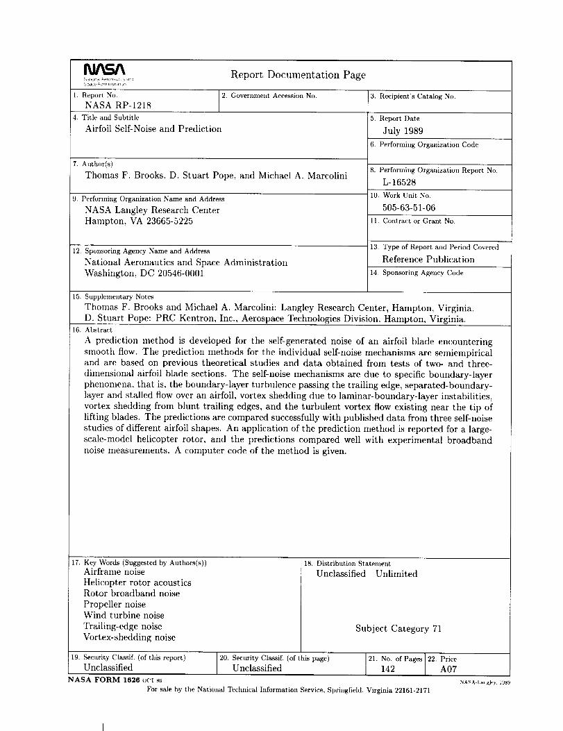
Report Documentation Page':; pac _- Adm,nisrraTlon
1. ReportNAsANO.RP_1218 [2. Government Accession No. 3. Recipient's Catalog No.
4. Title and Subtitle
Airfoil Self-Noise and Prediction
7. Author(s)
Thomas F. Brooks, D. Stuart Pope, and Michael A. Marcolini
5. Report Date
July 1989
6. Performing Organization Code
8. Performing Organization Report No.
L-16528
10. Work Unit No.
505-63-51-06
11. Contract or Grant No.
13. Type of Report and Period Covered
Reference Publication
14. Sponsoring Agency Code
9. Performing Organization Name and Address
NASA Langley Research Center
Hampton, VA 23665-5225
12. Sponsoring Agency Name and Address
National Aeronautics and Space Administration
Washington, DC 20546-0001
15. Supplementary Notes
Thomas F. Brooks and Michael A. Marcolini: Langley Research Center, Hampton, Virginia.
D. Stuart Pope: PRC Kentron, Inc., Aerospace Technologies Division, Hampton, Virginia.16. Abstract
A prediction method is developed for the self-generated noise of an airfoil blade encountering
smooth flow. The prediction methods for the individual self-noise mechanisms are semiempiricaland are based on previous theoretical studies and data obtained from tests of two- and three-
dimensional airfoil blade sections. The self-noise mechanisms are due to specific boundary-layer
phenomena, that is, the boundary-layer turbulence passing the trailing edge, separated-boundary-layer and stalled flow over an airfoil, vortex shedding due to laminar-boundary-layer instabilities,
vortex shedding from blunt trailing edges, and the turbulent vortex flow existing near the tip of
lifting blades. The predictions are compared successfully with published data from three self-noise
studies of different airfoil shapes. An application of the prediction method is reported for a large-
scale-model helicopter rotor, and the predictions compared well with experimental broadband
noise measurements. A computer code of the method is given.
17. Key Words (Suggested by Authors(s))Airframe noise
Helicopter rotor acousticsRotor broadband noise
Propeller noiseWind turbine noise
Trailing-edge noise
Vortex-shedding noise
18. Distribution Statement
Unclassified--Unlimited
Subject Category 71
19. Security Classif. (of this report)
Unclassified20. Security Classif. (of this page)
Unclassified 21. No. of Pages 22. Price142 A07NASA FORM 1626 OCT sG
For sale by the National Technical Information Service, Springfield, Virginia 22161-2171NASA Laugh. 1989