naval postgraduate school - apps.dtic.mil · it identifies ttps and mission profiles that achieve...

NAVAL POSTGRADUATE

SCHOOL

MONTEREY, CALIFORNIA

THESIS

Approved for public release; distribution is unlimited

AN INNOVATIVE APPROACH FOR THE DEVELOPMENT OF FUTURE MARINE CORPS

AMPHIBIOUS CAPABILITY

by

Jeffrey D. Parker, Jr.

June 2015

Thesis Co-Advisor: Susan M. Sanchez Paul T. Beery Second Reader Eugene P. Paulo

THIS PAGE INTENTIONALLY LEFT BLANK

i

REPORT DOCUMENTATION PAGE Form Approved OMB No. 0704–0188 Public reporting burden for this collection of information is estimated to average 1 hour per response, including the time for reviewing instruction, searching existing data sources, gathering and maintaining the data needed, and completing and reviewing the collection of information. Send comments regarding this burden estimate or any other aspect of this collection of information, including suggestions for reducing this burden, to Washington headquarters Services, Directorate for Information Operations and Reports, 1215 Jefferson Davis Highway, Suite 1204, Arlington, VA 22202-4302, and to the Office of Management and Budget, Paperwork Reduction Project (0704-0188) Washington, DC 20503. 1. AGENCY USE ONLY (Leave blank)

2. REPORT DATE June 2015

3. REPORT TYPE AND DATES COVERED Master’s Thesis

4. TITLE AND SUBTITLE AN INNOVATIVE APPROACH FOR THE DEVELOPMENT OF FUTURE MARINE CORPS AMPHIBIOUS CAPABILITY

5. FUNDING NUMBERS

6. AUTHOR(S) Jeffrey D. Parker, Jr. 7. PERFORMING ORGANIZATION NAME(S) AND ADDRESS(ES) Naval Postgraduate School Monterey, CA 93943-5000

8. PERFORMING ORGANIZATION REPORT NUMBER

9. SPONSORING /MONITORING AGENCY NAME(S) AND ADDRESS(ES) N/A

10. SPONSORING/MONITORING AGENCY REPORT NUMBER

11. SUPPLEMENTARY NOTES The views expressed in this thesis are those of the author and do not reflect the official policy or position of the Department of Defense or the U.S. Government. IRB Protocol number ____N/A____.

12a. DISTRIBUTION / AVAILABILITY STATEMENT Approved for public release; distribution is unlimited

12b. DISTRIBUTION CODE A

13. ABSTRACT (maximum 200 words)

The United States Marine Corps will bring toughness, vision, and refined tactics, techniques, and procedures (TTPs) from a 13-year desert fight into the next major combat operation or small contingency. This Marine Corps proclivity for action is reflected in driven Marines, doctrine and the personnel carriers or vehicles used by Marines to execute maneuver warfare from the sea. The first responder for the next contingency will likely be the Marine Expeditionary Unit (MEU), which is the smallest seabased configuration of a Marine Air Ground Task Force. The MEU provides rapid crisis response from U.S. Navy ships and is likely to be the principal component of the future force at sea. This research informs the top procurement priorities for the United States Navy by evaluating the MEU’s expeditionary amphibious assault capability and the use of ship-to-shore connectors. In hundreds of thousands of simulated assaults, it identifies TTPs and mission profiles that achieve increased operational effectiveness, while employing less operational energy. The major results quantify the benefits of debarking amphibious forces at closer distances, show that a self-deployer presents a significant advantage to the landing force, and reveal the diminishing returns of high water speed.

14. SUBJECT TERMS agent-based, dashboard, design of experiment, amphibious combat vehicle, MANA , robust solution, simulation, amphibious assault, data farming, ship-to-shore connectors

15. NUMBER OF PAGES

181 16. PRICE CODE

17. SECURITY CLASSIFICATION OF REPORT

Unclassified

18. SECURITY CLASSIFICATION OF THIS PAGE

Unclassified

19. SECURITY CLASSIFICATION OF ABSTRACT

Unclassified

20. LIMITATION OF ABSTRACT

UU NSN 7540–01-280-5500 Standard Form 298 (Rev. 2–89) Prescribed by ANSI Std. 239–18

ii


iii

Approved for public release; distribution is unlimited

AN INNOVATIVE APPROACH FOR THE DEVELOPMENT OF FUTURE MARINE CORPS AMPHIBIOUS CAPABILITY

Jeffrey D. Parker, Jr. Captain, United States Marine Corps

B.S., United States Naval Academy, 2006

Submitted in partial fulfillment of the requirements for the degree of

MASTER OF SCIENCE IN OPERATIONS RESEARCH

from the

NAVAL POSTGRADUATE SCHOOL June 2015

Author: Jeffrey D. Parker, Jr.

Approved by: Susan M. Sanchez Thesis Advisor

Paul T. Beery Co-Advisor

Eugene P. Paulo Second Reader

Robert F. Dell Chair, Department of Operations Research

iv


v

ABSTRACT

The United States Marine Corps will bring toughness, vision, and refined tactics,

techniques, and procedures (TTPs) from a 13-year desert fight into the next major combat

operation or small contingency. This Marine Corps proclivity for action is reflected in

driven Marines, doctrine and the personnel carriers or vehicles used by Marines to

execute maneuver warfare from the sea. The first responder for the next contingency will

likely be the Marine Expeditionary Unit (MEU), which is the smallest seabased

configuration of a Marine Air Ground Task Force. The MEU provides rapid crisis

response from U.S. Navy ships and is likely to be the principal component of the future

force at sea. This research informs the top procurement priorities for the United States

Navy by evaluating the MEU’s expeditionary amphibious assault capability and the use

of ship-to-shore connectors. In hundreds of thousands of simulated assaults, it identifies

TTPs and mission profiles that achieve increased operational effectiveness, while

employing less operational energy. The major results quantify the benefits of debarking

amphibious forces at closer distances, show that a self-deployer presents a significant

advantage to the landing force, and reveal the diminishing returns of high water speed.

vi


vii

TABLE OF CONTENTS

I. INTRODUCTION........................................................................................................1 A. PURPOSE .........................................................................................................1 B. BACKGROUND ..............................................................................................2 C. OBJECTIVES ..................................................................................................3 D. SCOPE ..............................................................................................................3

II. LITERATURE REVIEW ...........................................................................................5 A. AMPHIBIOUS OPERATIONS ......................................................................5

1. Distributed Combat Systems .................................................................7 2. The Role of Connectors in Amphibious Operations .........................8

3. Exploring the Reduction of Fuel Consumption for Ship-to-Shore Connectors of the Marine Expeditionary Brigade .................9

4. Operational Energy/Operational Effectiveness Investigation for Scalable Marine Expeditionary Brigade Forces in Contingency Response Scenarios......................................................10

B. GENERAL DESCRIPTION OF THE MARINE CORPS SCALABILITY AND AMPHIBIOUS ASSAULT ......................................12 1. The Environment ...............................................................................12 2. Marine Corps Background ...............................................................13

a. United States Marine Corps ....................................................13 b. Marine Expeditionary Brigade ...............................................14 c. Marine Expeditionary Unit .....................................................15

d. Sea Bases .................................................................................16 e. Distributed and Split Operations ............................................16 f. Operational Maneuver from the Sea ......................................17 g. Amphibious Assault ................................................................18

III. EW 12 SCENARIO AND MANA MODEL DEVELOPMENT ............................21 A. GENERAL DESCRIPTION .........................................................................21 B. MANA .............................................................................................................24

1. What is MANA? .................................................................................24

2. Benefits of MANA ..............................................................................24 3. MANA: Limitations and Assumptions ............................................25

a. Limitations of MANA..............................................................25

b. Assumptions Made in MANA .................................................26

C. RESEARCH QUESTIONS ...........................................................................26 D. MEASURES OF EFFECTIVENESS ...........................................................26 E. SCENARIOS ..................................................................................................27

1. Baseline Scenario (Scenario One) .....................................................27 2. Scenario Two ......................................................................................28 3. Scenario Three ...................................................................................29 4. Scenario Four .....................................................................................30

F. MODELING PARTICULARS .....................................................................31

viii

1. Theater of War—The Sea, Surf, Shore, and Land .........................31

2. Agents ..................................................................................................34 a. Blue Agent Properties .............................................................35 b. Red Agent Properties ..............................................................47

IV. DESIGN OF EXPERIMENTS .................................................................................49 A. GENERAL DESCRIPTION .........................................................................49

1. Factors and Ranges of Interest .........................................................50 a. Controllable Factors ...............................................................52 b. Uncontrollable Factors ...........................................................53 c. Robust Design .........................................................................54

B. NEARLY ORTHOGONAL AND BALANCED (NOB) MIXED DESIGNS ........................................................................................................54

C. EXECUTING THE EXPERIMENT ............................................................57 D. NUMBER OF REPLICATIONS ..................................................................58

V. DISTRIBUTED FLIGHT DECK OPERATIONS AND SIMIO MODEL DEVELOPMENT ......................................................................................................61 A. GENERAL DESCRIPTION .........................................................................61 B. SIMULATION MODELING FRAMEWORK BASED ON

INTELLIGENT OBJECTS ..........................................................................65 1. What is Simulation Modeling Framework Based on Intelligent

Objects? ..............................................................................................65 2. Benefits of Simio .................................................................................66 3. Simio: Limitations and Assumptions ...............................................66

a. Limitations of Simio ................................................................66

b. Assumptions Made in Simio ...................................................67 C. RESEARCH QUESTIONS ...........................................................................67 D. MEASURES OF EFFECTIVENESS ...........................................................68 E. SCENARIOS ..................................................................................................68 F. MODELING PARTICULARS .....................................................................69

1. Source ..................................................................................................69 2. Time-Varying Arrival Rate Table ....................................................70 3. Seabase ................................................................................................71

a. Launch Process: LHD ............................................................71 b. LPD ..........................................................................................72 c. Transit to the Objective Area, Objective Area Time on

Station, FARP Time and Sink ................................................72

VI. DATA ANALYSIS AND RESULTS ........................................................................75 A. JMP DATA ANALYSIS TOOL ...................................................................75

B. ANALYSIS OF AMPHIBIOUS ASSAULT EXPERIMENT ....................75 1. Histograms ..........................................................................................76

a. MOE (1): Blue Casualties.......................................................76 b. MOE (2): Red Casualties ........................................................77 c. MOE (3): Time to Attrite the Red Force to One-Third

Remaining Strength ................................................................78

ix

d. MOE (4): Force Exchange Ratio, Which is Calculated as

(Red Casualties +1)/(Blue Casualties +1) ..............................81 2. Box Plots .............................................................................................83

a. MOE (1) and MOE (2) ............................................................84 3. Statistical Tests to Compare Scenarios ............................................86

a. Scenario: Two-Sample t Test; One-Way Analysis of

Variance of Red Casualties by Scenario ................................87 4. Multiple Linear Regression Analysis ...............................................90

a. Main Effects ............................................................................91 b. Comparison of Main Effects...................................................94 c. Partition Trees .........................................................................97 d. Multiple Linear Regression Models .....................................101

5. Simio: Discrete-Event Simulation ..................................................109

VII. CONCLUSIONS AND RECOMMENDATIONS .................................................117 A. OVERVIEW .................................................................................................117 B. ENERGY INSIGHTS ..................................................................................118 C. OPERATIONAL INSIGHTS .....................................................................118

1. MOE Insights ...................................................................................120 D. FUTURE RESEARCH ................................................................................120 E. SUMMARY ..................................................................................................121

APPENDIX A. COMPLETE TABLE OF BLUE SQUADS ............................................123

APPENDIX C. COLLAPSED DATA BY SCENARIO, PAIRED ..................................127

APPENDIX D. RAW OUTPUT DATA, PAIRED ............................................................129

APPENDIX E. MULTIPLE LINEAR REGRESSION COMPARISON TABLE .........131

APPENDIX F. “TIME” MOE, MULTIPLE LINEAR REGRESSION, ASSUMPTIONS .......................................................................................................135

APPENDIX G. ALL 77 MIXED (CONTINUOUS AND DISCRETE) FACTORS .......137

APPENDIX H. MEANS COMPARISON USING STUDENT T-TEST .........................139

APPENDIX I. SIMIO AND MANA DASHBOARD COMPARISON ............................141

APPENDIX J. APPROACH, MODEL-TEST-MODEL ..................................................143

LIST OF REFERENCES ....................................................................................................145

INITIAL DISTRIBUTION LIST .......................................................................................149

x


xi

LIST OF FIGURES

Figure 1. QRF/Close Air Support (CAS) Insertion, MEDEVAC, and QRF/CAS Withdrawal for 3-Platoon, 4-Platoon, and 5-Platoon have higher Fuel Mission Use than Close Air Support, Logistics Resupply, and Ground Mission (from Team Expeditionary & Cohort 311-132, 2014). ......................11

Figure 2. An AAV debarking from an amphibious assault ship USS Bataan (LHD-5). AAVs in operation today are over 40 years old (from Eckstein, 2015). ....18

Figure 3. Assault Amphibian Modernization projections from 2014 to 2034. Approximately 700 ACVs (wheeled, bottom right), totaling six companies, are to be procured to replace the bulk of the legacy AAV (tracked, upper left). Nearly 400 of the AAVs are to receive an upgrade (from LaGrone, 2015). .....................................................................................19

Figure 4. Enemy ground threat situation (from Wargaming Division, 2012). ................22 Figure 5. CJTF CONOP, Phases I-III (from Wargaming Division, 2012). ....................23 Figure 6. Four LCACs or SSCs “+” returning to the seabase after bringing Blue

ashore. ..............................................................................................................28 Figure 7. Four SSCs, capable of 4xACV or 1xM1A1 “LCAC loads.” The MANA

icon used for the LCAC is “+,” during a wave ashore, this icon will be overlayed by numerous icons of ACVs, M1A1 tanks, and equipment. Wave one is accompanied by AAVs. ..............................................................29

Figure 8. Heliborne raid of MV-22 aircraft from the seabase. ........................................30 Figure 9. Heliborne raid and wave one supported by AAVs. .........................................31 Figure 10. Terrain map, including the red, green, and blue (RGB) colors with dark

green shown at right. ........................................................................................32 Figure 11. In order to mass force ashore prior to moving deeper into the threat

environment, agents must press inland and establish security (pink). Agents next await the final wave. As the final wave arrives squad 42, an agent representing CAAT, refuels friends, which cause the advance (green). .............................................................................................................33

Figure 12. LHD Agent: Depicts the GUI for in MANA. The agent icon is located in the lower left, possible trigger states (e.g., Default State, Reach Final Waypoint) are in a column to the right. ...........................................................37

Figure 13. Baseline factor of four LCACs as the SSC. The bottom right square shows the fourth LCAC on the first wave loaded with four ACV. The squad number is 73 for that particular LCAC. One may alter the design features of these “black box LCAC” to upgrade this modeled agent capability to JHSV, UHAC, “Mike Boats” (LCM-8), LCU, concept LCAC, etc. ...............38

Figure 14. LCAC Agent: Depicts the Personalities GUI in MANA. The agent icon is located in the lower left, possible trigger states (e.g., Default State, Reach Waypoint, Reach Final Waypoint, Run Start) have a check in the box. The Run Start trigger state is unique to the LCAC, as their waves are based on time. .................................................................................................................39

xii

Figure 15. ACV agent: Depicts the GUI for in MANA. Trigger states used are the Default State, Reach Waypoint, Refuel By Friend, and Reach Final Waypoint. Run start is not required as the ACV are debussed from LCAC when the LCAC reaches its debark point. .......................................................42

Figure 16. ACV agent, tangibles shown are number of hits to kill, movement speed, allegiance, threat level, and agent class. ..........................................................43

Figure 17. ACV agent, detection and classification range and probability shown. .........43 Figure 18. ACV agent, depicts weapon ranges, probability of hit, round count, reload

time, target priority list. ...................................................................................44 Figure 19. CAAT agent called AntiTankTm1, represented in pink, has a personality

weight to move toward Red tanks. Once released from emboss, the agent seeks to Refuel Friends (see: Section C of this chapter). .................................45

Figure 20. Red tanks, anti-tank teams, ADA, and infantry. ..............................................47

Figure 21. Experiment setup schematic, which shows the four scenarios and two other decision factors: (1) distance from shore that ACVs are deployed from the SSCs, and (2) the number of SSCs. ...................................................49

Figure 22. A schematic of how the simulation’s landing plan was adjusted to accommodate 2, 3, and 4 LCACs. ...................................................................53

Figure 23. The top row features factorial designs and the bottom row illustrates the near-orthogonality and space-filling properties of NOLH designs (from Sanchez, Sanchez, & Wan, 2014). ...................................................................55

Figure 24. An excerpt of the 512-design point, NOB design spreadsheet template, which allows for the investigation of the 77 factors. The template can handle simultaneous investigation of 300 factors, with discrete number levels and continuous-valued factors (after Sanchez, Sanchez, & Wan, 2014). ...............................................................................................................56

Figure 25. Color map of the design’s pairwise correlations..............................................57 Figure 26. Confidence interval half-width diminishing returns, based on the number

of replications. It appears that the added benefit from going from 30 replications to 100 might not be worth the computational cost of running a MANA simulation that takes 10 minutes, on average, for each simulation. ...59

Figure 27. Figure 28 shows an MV-22 Osprey launching from a forward spot. All three aircraft, to include the CH-53E, belong to Marine Medium Tiltrotor Squadron (VMM) 265 (Reinforced) (from Achterling, 2014). ........................62

Figure 28. MV-22 Ospreys with folded rotors and wings in the forward and aft “slash” of the LHD (from Galante, 2009). .......................................................63

Figure 29. MV-22 Ospreys at night occupying all four of the expanded spots on the amphibious transport dock ship USS Mesa Verde (LPD 19). Expanded spots three and six have turning aircraft, preparing for launch, and expanded spots four and five have MV-22s with their rotors and wings folded. These aircraft are assigned to the 22nd MEU and the picture was taken during a composite training unit exercise (COMPTUEX) in preparation for a deployment (from Smith, 2013). .........................................64

Figure 30. Marine forces from the 11th MEU cross the flight deck to the five MV-22 Ospreys attached to Marine Medium Tiltrotor Squadron 163 (Reinforced).

xiii

The flight deck is that of the amphibious assault ship USS Makin Island (LHD-8) (from Fuentes, 2015). .......................................................................65

Figure 31. Screen shot of the Simio simulation. ...............................................................73 Figure 32. Histograms of Blue casualties by scenario. The highest mean of Blue

casualties occurs for scenario 3. Recall that scenario 3 conducts STOM-V, with a wave of MV-22s. Scenario 4 combines scenarios 2 and 3, so it also shows a high mean number of casualties compared to scenarios 1 and 2. ......76

Figure 33. Red casualties are greatest when Blue attacks with ACVs and AAVs in both scenarios 2 and 4. Red’s survival is better when Blue does not use the AAVs. Red casualties experience little change from scenario 1 to 3. Scenarios 2 and 4, each have waves of AAVs accompanying ACVs onboard LCACs. ..............................................................................................77

Figure 34. Time to attrite the Red force to one-third remaining strength, where the fastest mean time occurs with scenario 4. This objective is not met 84 times with scenario 1 (512 – 428 = 84). Meanwhile, scenario 2 has the lowest standard deviation and higher times can be expected with scenario 3, seen in the circled portion of the data. .........................................................78

Figure 35. Realized probability for attriting Red to one-third of its remaining forces. ....80 Figure 36. FER MOE. This is calculated as (Red casualties +1)/(Blue casualties +1)

with the raw data. Higher values imply that Red experienced greater casualties than Blue. Blue achieves the highest FER with scenarios 2 and 1........................................................................................................................81

Figure 37. FER MOE with raw output data. Highest is scenario 2 and the lowest is scenario 3. ........................................................................................................82

Figure 38. Relationship between Blue casualties (y-axis) and FER (top), by scenario. Higher Blue casualties are seen at the far left when FER is the lowest. ..........83

Figure 39. Depicted is a box plot. Box plots in JMP have whiskers that extend out to 1.5 times the interquartile range (IQR). The boxed region shaded in gray represents the IQR, bounded by the 25th and 75th quantiles. JMP depicts outliers with large dots that fall outside of 1.5 times the IQR (from Lucas, 2014). ...............................................................................................................84

Figure 40. This figure shows that there is little difference for Red between scenarios 2 and 4, while Blue incurs many more casualties in scenarios 3 and 4. ..........84

Figure 41. The Blue casualties’ plot on the left shows that Blue casualties are more influenced by scenario than by debark distance or number of LCACs. The Red casualties’ plot on the right shows that Red casualties are influenced by debark distance, LCAC count, and scenario. ..............................................85

Figure 42. Blue casualties during scenarios 3 and 4 are attributed mostly to those infantry arriving via MV-22s, STOM-V. .........................................................86

Figure 43. This plot shows a one-way analysis of the summarized output (2,048 rows) for “Red casualties” by scenario, with the number of Red casualties on the vertical axis. In red, we see overlapping circles for scenarios 1 and 3. Scenarios 2 and 4 have similar boxplots and circles which are “overlapped.” ...................................................................................................88

Figure 44. Connecting Letters Report at the 95% confidence level. .................................88

xiv

Figure 45. The Ordered Differences Report. .....................................................................89

Figure 46. One-way analysis of Red casualties, based on the full set of outputs. .............90 Figure 47. Full uncompressed output, “Blue casualties.” Scenario 3 increases “Blue

casualties,” while scenarios 2 and 1 decrease “Blue casualties.” ....................91 Figure 48. Full uncompressed output, “Red casualties” depend on ACV speed,

debark distance, LCAC quantity, and LCAC speed. .......................................92 Figure 49. Red casualties increase with all three speeds: LCAC, AAV, and ACV.

Similarly, scenarios 2 and 4, and LCAC quantities of three and four increase the number of Red casualties. “Red casualties” decrease when the ACVs are debarked further than 12 nm from the shore. ..................................92

Figure 50. “Time” MOE. ACV speed contributes most to reducing the “time to attrite Red Force to one-third remaining strength.” Debark distances and scenario 1 take longer to attrite Red to the desired level. ..............................................93

Figure 51. The “time” MOE and how scenario, ACV debark distance, and LCAC quantity compare. .............................................................................................94

Figure 52. The main effect models for Blue and Red casualties. ......................................94 Figure 53. The main effect models for FER and “time” MOE. ........................................95 Figure 54. “Blue casualties” partition tree. .......................................................................98 Figure 55. Blue casualties’ partition tree, split history for mean Blue casualties, the

black vertical line at eight splits shows little increased R squared from the four splits show previously. .............................................................................99

Figure 56. “Red casualties” partition tree, most import split ACV speed greater than 16 knots (18 mph). .........................................................................................100

Figure 57. Red casualties’ partition tree, where more splits might explain more of the variance. .........................................................................................................101

Figure 58. R square vs. p (number of parameters) for “Blue casualties” on the left and “Red casualties” on the right..........................................................................102

Figure 59. R square vs. p (number of parameters) for “time” on the left and “FER” on the right. .........................................................................................................102

Figure 60. Predicted mean blue casualties, with actual observations shown with black dots. The dashed blue line depicts the average blue casualties......................104

Figure 61. Mean “Blue casualties” summary of fit. The R squared is 55%, and the R squared adjusted is 55%, implying that over half of the variation is explained by this model. ................................................................................104

Figure 62. Mean “Blue casualties” sorted parameter estimates. .....................................105 Figure 63. Mean “Blue casualties” MOE, prediction profiler. Force protection and

ACV sensor range reduce Blue casualties and scenario increase the number of casualties. The x-axis is the number of hits, range (meters), and scenario for the main effects. The y-axis is the mean number of casualties. .106

Figure 64. Pareto plot for “Blue casualties.” The curved line supports that little additional variance will be gained with increased degrees of freedom or more parameters. ............................................................................................107

Figure 65. The Simio experiment had three primary scenarios, run with 1,000 replications, one control “prop_LHA,” a response. The response is “Mission Total Time.” ...................................................................................109

xv

Figure 66. Pivot table in Simio, the category “Holding Time” had to be extracted from the entire data set for all scenarios only all aircraft launching from LHA and disaggregated operations being show (all_LHA and disaggOps). .110

Figure 67. Mean mission holding hours for 14 aircraft launching from the LHA only, 0.32 hours. ......................................................................................................110

Figure 68. Mean mission holding hours, all aircraft, during split operations, 0.29 hours. ..............................................................................................................111

Figure 69. Mean mission holding hours, all aircraft, during disaggregated operations, 0.28 hours. ......................................................................................................111

Figure 70. STOM-V graph of increased casualties with scenario 3. ...............................112 Figure 71. The bar graph shows pounds of fuel burned per sortie. A sortie is defined

as one hour of flight launched from a ship. ...................................................113 Figure 72. Assault aircraft on a MEU deployment at three levels of deployment

intensity consisting of 6-, 24-, or 48-raid missions. .......................................114 Figure 73. After 10 years, potential DOD savings from fuel. Interest rate of return 3

%. Annual savings for split and disaggregated, $1.93 M split and $1.98 M for disaggregated. ...........................................................................................115

Figure 74. After 1,000 replications, practically no significant effect on mission time. ..116 Figure 75. What is the most important vehicle type in an amphibious assault? Of the

four scenarios, scenario 3 masses Blue force the fastest with the MV-22; however, dismounted infantry are not afforded the same protection as those inside vehicles like the ACV and AAV. ...............................................119

Figure 76. Shows the FER, by scenario, with the non-collapsed data. ...........................125 Figure 77. One-way analysis of mean “Red casualties” MOE by scenario. ...................127 Figure 78. One-way analysis of the mean “Red casualties” MOE by scenario with the

non-collapsed output data. .............................................................................129 Figure 80. MOE “Blue casualties” actual by predicted, summary of fit, prediction

profiler, and Pareto plots. ...............................................................................131 Figure 81. MOE “Red casualties” summary of fit, sorted parameter estimates,

prediction profiler, and Pareto plots. ..............................................................132 Figure 82. MOE “time” summary of fit, sorted parameter estimates, prediction

profiler, and Pareto plots. ...............................................................................133 Figure 83. MOE “FER” sorted parameter estimates, prediction profiler, and Pareto

plots. ...............................................................................................................134 Figure 84. MOE “time” advanced regression model, normal Q-Q plot, closely fits

along the line, passes the “fat pencil test.” .....................................................135

Figure 86. Complete NOB, 77 factor DOE. ....................................................................137

Figure 87. Screen grab of the 12 factors combined using the techniques described from Efficient, nearly orthogonal-and-balanced, mixed designs: an effective way to conduct trade-off analyses via simulation. Retrieved from Vieira, 2013....................................................................................................138

Figure 88. T Means comparison for statistically significant scenarios using student t-Test. ................................................................................................................139

Figure 89. Paired comparison, scenarios two and four for statistical significance .........140 Figure 90. Screen shot of Simio dashboard .....................................................................141

xvi

Figure 91. Screen shot of terrain billboard in MANA. ...................................................141

Figure 92. An illustration of the model-test-model approach, see chapter III for actual concept of operations and scenario development. .........................................143

xvii

LIST OF TABLES

Table 1. MANA Agent Classifications. .........................................................................34 Table 2. This table shows the four M1A1 tanks and 19 ACVs modeled. The table

also shows the LCAC squad number or parent agent that brings them ashore. For example, ACV-P-1, ACV-P-2, & ACV-P-3 and the Recovery ACV (squad 93, ACV-R-1) all have the same parent. .....................................35

Table 3. Complete listing of Blue experiment factors. ..................................................51 Table 4. Complete listing of Red experiment factors. ...................................................52 Table 5. The three options modeled are: all aircraft launching from the LHD, the

split, and disaggregated operations. Aircraft launched from the LHD have two slashes (forward and aft), three spots, and one crew to facilitate the launch sequence. No LPD slash, spots, or crew are available in “all from LHD” operations. .............................................................................................69

Table 6. This Time Varying Arrival Rate Table shows the launch of a section of AHs within the first 30 minutes of flight operations, followed by the GCE aboard six MV-22s in the next 30 minutes, followed by the SAR, FARP, and command and control aircraft, until, lastly, the F-35Bs are launched. .....71

Table 7. This is a summary of the multiple regression models explored for MOEs 1-4. .................................................................................................................108

Table 8. The top line has all LHA, split, and disaggregated operations. Below are the low, operational planning, and high end burn rates in one table (i.e., “lo,” ”Planning,” and “hi”). These numbers provide a range for a decision maker..............................................................................................................113

Table 9. Complete table of the 113 Blue squads in MANA. .......................................123

xviii


xix

LIST OF ACRONYMS AND ABBREVIATIONS

A2/AD anti-access/area-denial

AAV Amphibious Assault Vehicle

ACE Aviation Combat Element

ACV Amphibious Combat Vehicle

ADA air defense artillery

ANOVA analysis of variance

AoA Analysis of Alternatives

AoR Area of Responsibility

APC armored personnel carrier

APOD air point of debarkation

ARG Amphibious Ready Group

ATF Amphibious Task Force

BLT battalion landing team

BN battalion

C2 command and control

CAAT combined anti-armor team

CAS close air support

CASEVAC casualty evacuation

CATF Commander Amphibious Task Force

CERTEX certification exercise

CI confidence interval

CJTF Combined joint Task Force

CLF Commander, Landing Force (CLF)

CMC Commandant of the Marine Corps

COMPTUEX Composite Training Unit Exercise

CONOP concept of operation

CR crisis response

CSV comma-separated values

xx

DC displacement craft

DES discrete-event simulation

DOD Department of Defense

DOE design of experiments

E2O Expeditionary Energy Office

EF-21 Expeditionary Force 21

EFSS Expeditionary Fire Support System

EFV Expeditionary Fighting Vehicle

ESG Expeditionary Strike Group

EW 12 Expeditionary Warrior 2012

FARP forward arming and refuel points

FCS Future Combat Systems

FER force exchange ratio

FLOT forward line of troops

FOC full operational capability

FPR final project review

FSM Free Savanna Movement

FT fire team

GB gigabyte

GCE Ground Combat Element

GUI graphical user interface

HA/DR Humanitarian Aid and Disaster Relief

HMMWV High Mobility Multipurpose Wheeled Vehicle

hr hour

ICD initial capabilities document

IED improvised explosive device

IEEE Institute of Electrical and Electronics Engineers

Inf Infantry

IOC initial operating capability

IQR interquartile range

xxi

JFEO joint forcible entry operation

JHSV Joint High Speed Vessel

JP-5 jet propellant 5

km/hr kilometers per hour

kts knots

LAVGrp light armored vehicle group

lbs pounds

LCAC landing craft air cushion

LCU landing craft unit

LF landing force

LHA amphibious assault ship (general purpose)

LHD amphibious assault ship (multipurpose)

LPD amphibious transport dock

LSD dock landing ship

m meters

MAGTF Marine Air Ground Task Force

MANA Map Aware Non-Uniform Automata

Max maximum

MCDP Marine Corps Doctrinal Publication

MCO major combat operation

MEB Marine Expeditionary Brigade

MEDEVAC Medical Evacuation

MET Mission Essential Task

MEU Marine Expeditionary Unit

Min minimum

MLP Maritime Landing Platform

mm millimeter

MOE measure of effectiveness

MOP measures of performance

MPC Marine Personnel Carrier

xxii

mph miles per hour

MRAP Mine-Resistant Ambush Protected

nm nautical miles

No. number

NOB nearly orthogonal-and-balanced

NOLH nearly orthogonal Latin hypercubes

NPS Naval Postgraduate School

OE2 Operational Energy/Operational Effectiveness

OEF Operation ENDURING FREEDOM

OIF Operation IRAQI FREEDOM

OMFTS operational maneuver from the sea

Ops operations

OR operations research

OTH over the horizon

QRF quick reaction force

RAM random-access memory

RGB red, green, and blue

ROMO range of military operations

RWS remote weapon station

SAR search and rescue

SAS Suite of Analytics Software

SBME sea-based maneuver echelon

SE systems engineering

SEED Simulation Experiments & Efficient Designs

Simio SImulation Modeling framework based on Intelligent Objects

SLEP service life extension program

SOC special operations capable

SOM scheme of maneuver

SPMAGTF-CR Special Purpose MAGTF-Crisis Response

SPOD sea point of debarkation

xxiii

SSC ship-to-shore connector

STOM Ship-to-Objective Maneuver

STOM-V/S Ship-to-Objective Maneuver-vertically/surface

T/M/S Type/Model/Series

TOS time on station

TOW tube-launched, optically tracked, wire-guided

TRL technology readiness level

UAMBL Unit of Action Maneuver Battle Lab

UHAC Ultra Heavy-lift Amphibious Connector

U.N. United Nations

USMC United States Marine Corps

USS United States Ship

VBA visual basic for applications

VBSS visit, board, search, and seizure

VMM Marine Medium Tiltrotor Squadron

WAF West African Federation

WBS work breakdown structure

XML EXtensible Markup Language

xxiv


xxv

EXECUTIVE SUMMARY

In the wake of cost overruns the Expeditionary Fighting Vehicle in 2011 was

terminated, and the U.S. Marine Corp transitioned to a tough amphibian, the Amphibious

Combat Vehicle (ACV). This vehicle, in its current increment, will leverage ship-to-shore

connectors (SSCs) to meet the challenges presented from objective maneuver from the

sea (OMFTS). Marines perform amphibious operations with forces that are scalable and

tailorable, meaning that these operations may elevate from a benign landing (e.g., New

Orleans during Katrina) to a joint forcible entry operation (e.g., Omaha Beach) on distant

shore. Incidentally, amphibious operations are highly complex, which raises many

questions:

Does the U.S. Marine corps require a self-deploying capability similar to the legacy Amphibious Assault Vehicle (AAV), which conducts ship to objective maneuver (STOM)?

What are the right measures of performance (MOP) for an amphibious operation, namely a system of connectors delivering many systems of amphibious combat vehicles?

What ranges from the shore and speeds present challenges to an amphibious operation given modern technology?

What are the impacts and drivers of operational energy and how can the U.S. Marine Corps maintain mission effectiveness?

Are there solutions that afford the same operational effectiveness, yet reduce operational energy from the seabase being distributed?

This research uses a two-stage simulation to model an end-to-end amphibious

assault, which addresses these questions. The sponsor for this research was the

Expeditionary Energy Office (E2O), USMC. Initial progress reviews revealed that the

Marine Corps has many spreadsheet-based and specific tools; however, the stakeholder

needed a broad analysis of expeditionary operations. The top acquisitions priority for the

Marine Corps pertains to Title 10 amphibious requirements. Thus, a broad analysis for an

amphibious operation is conducted. A discrete event simulation in a Simulation Modeling

framework based on Intelligent Objects (Simio) models aircraft launch constraints from

xxvi

the seabase. Meanwhile, an agent-based adversarial model in Map Aware Non-Uniform

Automata (MANA) models the amphibious assault.

Once the model structure was established, the author used a model-test-model

approach that refined terrain, adversary capabilities, and landing force scheme of

maneuver (SOM) to gain operational insights. Many hundreds of thousands of simulated

amphibious assaults were conducted with a broad range of parameters in efficient, space-

filling experiments, involving 77 mixed (i.e., discrete and continuous) factors with 512

design points for four different scenarios. Run times for a single experiment took

approximately 10 minutes, so the excursions were completed using a high-performance

computing cluster. In the end, advanced metamodels were selected from linear, non-

linear, regression, and partition tree analyses.

The ACV, AAV upgrade, and next SSC all present major Department of Defense

programmatic decisions. This research informs these decisions leveraging a traceable

scenario throughout to better assist decision makers in providing the warfighter the right

capabilities. The major findings follow.

STOM-vertically (STOM-V) presents a future challenge for the Marine Corp—not in the distance that can be covered, but in the force protection provided to Marines once on the ground.

The adversary will be highly influenced by the ends, ways, and means of an attacking force during amphibious assault.

The ACV swim and on-land speed do not need to be as fast as current top capabilities.

An ACV with an autonomous ship-to-shore increment (i.e., self-deployer) presents a significant advantage to the landing force.

Distances offshore can range as far as 12 nm without interference to the amphibious assault.

Different types of urban terrain may degrade the defending forces ability to target the landing force.

This thesis provides an innovative approach for developing meta-models of

operational effectiveness. These meta-models are part of a prototype “dashboard” for

xxvii

E2O that links operational effectiveness and operational energy to facilitate trade-space

explorations.

In summary, the force that responds to the next crisis or contingency will be the

force that is closest to it—the Marine Expeditionary Units (MEUs) embarked on ships.

This research is leaning forward by making a first attempt at modeling an end-to-end

amphibious assault. In hundreds of thousands of simulated amphibious assaults, we

observe the trade-space formed by the many complex parameters considered when

employing concept complementary platforms of surface and vertical ship-to-objective-

maneuver. In the end, we realize quantifiable values that maximize mission effectiveness

and better inform the top procurement priorities for the United States Naval forces.

xxviii


xxix

ACKNOWLEDGMENTS

I am so thankful for my supportive wife and our family. To my wife, Chrissie,

thank you for your love and unwavering support. To my parents, sister, and my wife’s

family—thank you for helping watch our “three-little-ones-under-three.” Your support is

greatly appreciated.

Furthermore, this research would not have been made possible had it not been for

Professor Eugene Paulo and Mr. Paul Beery including me in their capstone projects; this,

pooled with a willingness to combine systems engineering and operations research work,

has created a thesis of impact for the United States Marine Corps.

I want to especially thank my advisors, Professor Susan Sanchez and the

aforementioned Paul Beery, for all of their guidance, suggestions, and support. I feel very

fortunate to have spent such quality time with advisors so dedicated to their students.

Likewise, I want to thank Mary McDonald for her help with the super cluster, MANA-V,

and all the analysis therein—without her support, such a complex system could not have

been accurately modeled.

This research is dedicated to the many fallen Marines and those who will never

forget them. On January 23, 2015 two Camp Pendleton Marines were killed flying a UH-

1Y. Less than two months later, on March 13, 2015, seven United States Marine Corps

Forces Special Operations Command (MARSOC) Marines were lost off the coast of

Florida in a helicopter crash. And, most recently—six Marines and two Nepalese soldiers

were killed in Nepal on May 12, 2015. Our heartfelt thoughts and prayers go out to their

families and loved ones.

xxx


1

I. INTRODUCTION

The farther backward you can look, the farther forward you can see

—Winston Churchill Prime Minister of the United Kingdom,

October 1951–April 1955

A. PURPOSE

The purpose of this research is to further analyze complex, amphibious operations

in anti-access/area-denial (A2/AD) situations, based on a traceable scenario, in order to

provide a tool for decision makers to explore operational effectiveness and operational

energy in amphibious operations. The United States Marine Corps (USMC) has been

using amphibious vehicles for launching assaults from the sea since 1776, but modern-

day circumstances are driving the need for an agent-based tool—primarily, the advent of

expensive technology in the amphibious vehicle capability and the variety of equipment

that can be based at sea against an adaptive adversary. The Marine Corps can explore

new technology based at sea in a cost-effective environment that allows stakeholders to

visualize billions of dollars of equipment prior to it being procured. This thesis uses

campaign analysis techniques, agent-based simulation, and discrete event simulation in a

broad analysis of conceptual ship-to-shore connectors and developing Marine amphibious

combat vehicle technology during a seabased amphibious assault.

The principal arm for scalable Marine amphibious operations is the Marine

Expeditionary Unit (MEU). In order to provide rapid crisis response from U.S. Navy

ships, the MEU must be highly trained to this end, the over 2,200 Marines and hundreds

of aircraft in a MEU regularly conduct a minimum of six months of work-ups, followed

by certification-at-sea periods, and deployments around the globe. The principal benefit

of this thesis is incorporating the findings of this research and applying them to

persistent, regularly scheduled operations. Findings that, once applied to all seven of the

currently active MEUs, may very well influence operational energy consumption for the

United States. This effect would be multiplied annually by the three operational and four

in reserves, rotation cycle of the MEU. Even MEUs that are not deployed operationally,

2

those conducting work-ups to replace them, conduct hundreds of theater security

cooperation and training operations. Furthermore, the agent-based model employed in

this analysis is unlike any other—for it models that which has been too complex to model

until now—amphibious assault.

B. BACKGROUND

The amphibious combat community is highly capable, and the aim of this

research is to help inform the vision of the future amphibious assault force. To better

serve the leadership of Marines fighting in future wars and to aid in making better data-

driven decisions, this model tackles what has been avoided for too long due to

complexity—modeling the amphibious assault. Marines need a tool that attacks the

complex, ship-to-shore amphibious transition with the same level of intensity that they

will be expected to produce when they launch an amphibious assault. Additional

motivation for this thesis stems from combined research between the Operations

Research (OR) and Systems Engineering (SE) Departments at the Naval Postgraduate

School (NPS). Professors from both departments at NPS have dedicated much of their

research to providing a dashboard for the United States Marine Corps that uses ensembles

of models, commonly referred to as metamodels, to show operational energy and

operational effectiveness. The author is incorporating work from a year-long SE

capstone, Operational Energy/Operational Effectiveness Investigation for Scalable

Marine Expeditionary Brigade Forces in Contingency Response Scenarios (Team

Expeditionary & Cohort 311-132, 2014) to further investigate the feasibility of using

amphibious assault operations with future programs and technology, such as concept

ship-to-shore connectors (SSCs), amphibious combat vehicles (ACVs) and other Marine

Personnel Carriers (MPCs). Sponsoring this research is the Marine Corp’s Expeditionary

Energy Office (E2O). In 2009, then Commandant of the Marine Corps (CMC), James T.

Conway, formed E2O to “analyze, develop, and direct the Marine Corps’ energy strategy

in order to optimize expeditionary capabilities across all warfighting functions” (Marine

Corps Expeditionary Energy Office [E2O], 2012). The modeling implemented in this

thesis is currently being used by a second systems engineering research team in support

of their master’s research, and lays the groundwork for further studies as well.

3

C. OBJECTIVES

This research is guided by the following research questions, whereby the

measures of effectiveness (MOEs) are mission time, friendly casualties, and Red

casualties:

What are the ACV measures of performance (MOPs) that positively contribute to the MOEs?

What are the SSC MOPs that positively contribute to the MOEs?

While we do not know exactly what enemies future Marine amphibious combat

systems will face, it would be unwise to assume away the threat and that future adversary

as being anything less than formidable, adaptive, and located deep inside a complex

coastal defense. While the U.S. has invested in ships, other states have taken advantage of

more affordable coastal defense missile systems. The natural defense created by the

terrain of sea, surf, and sand gives an edge to the enemy. This is further complicated by

asymmetric threats, A2/AD capabilities, and modern warfare technologies, making it

difficult for decision makers to select the right capabilities amid uncertainty. In order for

Marine leadership to continue to function and successfully conduct amphibious assault

operations, new technology must be robust to a variety of missions and scenarios. This

research delivers results, facts, and a tool for the future rapid, data-driven decision

making—appropriate for Marines to adopt and use to destroy the enemy.

D. SCOPE

The primary focus of this thesis is to quantify the benefits of distributing assets

among platforms found in seabase operations during an amphibious assault. In support of

that focus, this thesis develops a visualization tool of the amphibious assault operation.

This thesis uses agent based simulation software, Map Aware Non-uniform Automata

(MANA, version 5.0 [V]), and discrete event simulation software, SImulation Modeling

framework based on Intelligent Objects (Simio, version 7.0), to develop scenarios and

simulations. The MANA and Simio scenarios and simulations used work well with

numerous vertical and surface Marine platforms. The Simio simulation is particularly

useful to realize the benefit to operating Marine aircraft distributed across air capable

4

ships. Meanwhile, the MANA scenario uses a large number of agents and decision

factors to model everything from an M1A1 tank, to an SSC, to a Marine infantry fire

team (FT).

The following five chapters develop an innovative approach for the expansion of

future Marine Corps amphibious capability using simulation modeling. Amphibious

operations require logistics. As a result, others have developed several limited tools

implementing visual basic for applications (VBA) and discrete-event simulations (DES)

to calculate massing force ashore absent the enemy. These tools may include stochastic

elements, but are incapable of providing insight when an adaptive adversary is present. In

contrast, the research in this thesis is unique, combining both discrete and agent-based

simulations to explore a range of specifications and impacts on operational energy and

operational effectiveness in likely amphibious scenarios against an enemy. Chapters I and

II introduce the research and the approaches made by others to model amphibious

operations. Chapters III and IV cover the two simulation methodologies, namely agent

based and discrete-event simulations. Chapter VI and VII cover the quantitative analysis,

conclusions, and recommendations as they pertain to energy insights, operational

insights, and future work.

5

II. LITERATURE REVIEW

A. AMPHIBIOUS OPERATIONS

There is much written from great and experienced military theorists, such as

Sun Tzu, Carl Von Clausewitz, and Alfred Thayer Mahan, which the U.S. Armed Forces

use to be prepared for positions of operational leadership, and to think strategically about

all types of wars and the means used fight them (U.S. Naval War College, 2015). While

all three theorists may not agree on how best to conduct forcible entry from the sea,

Griffith’s rendition of Sun Tzu’s ‘The Art of War’ says, “attack where he is unprepared,”

and seabased forces provide this capability (Griffith, 1971, p. 69). Where disagreement

may also arise is, which of the multifaceted technologies of today best help accomplish

this mission? Undoubtedly, what is not covered by history is modern-day, complex,

concept platform integration. Developments of new SSCs and armored personnel carriers

(APCs) (e.g., ACVs, MPCs, etc.) can be defined in terms of specifications and system

performance, typically quantified as MOPs. Yet, it is often the systems of systems that

contribute toward mission accomplishment, typically quantified as MOEs. Amphibious

assault, and the technological advancements made therein, present unique challenges to

the adversary. Platform-intensive operations, however, significantly increase the

complexity of battle. So, while belligerent nations must defend their coasts against a

hovercraft that can carry a formidable force quickly from well over the horizon (OTH),

this capable connector is susceptible to battle damage and breaking down. If we assume

no battle damage to vehicles, and no personnel destroyed, as with most DESs and

calculators, then we fail to capture what centuries of theorists have been saying not to

discount—the enemy. Hence, this research considers the impact of the enemy on the

mission, rather than MOPs that only focus on the isolated performance of each system.

A counter argument to logistic calculators and complex platforms is the impact of

U.S. Marine Corps leadership, bravery, and experience—all of which provide a

formidable edge that is unquantifiable. The Marine Corps history of amphibious

operations stretches from 1776 to 2006. While the Bahamas in 1776 represent the first

amphibious operation, Veracruz, in 1846, was the first major joint amphibious operation.

6

Marine Captain Alvin Edson led a battalion (BN) of Marines on 9 March 1846, thus

executing the first joint forcible entry operation (JFEO), with the support of over 8,000

soldiers, sailors, and Marines (U.S. History., 2015). Few real-time analysis tools have

been made with the modernizations of amphibious assault technology in mind. As we

explore past studies, according to Clausewitz’s On War: “Critical analysis is not just an

evaluation of the means actually employed, but of all possible means—which first have to

be formulated, that is, invented. One can, after all, not condemn a method without being

able to suggest a better alternative” (Howard, Paret, & West, 1984, p. 161). To this end,

this research aims to build on other work that incorporates a vast breadth of research

investment into making the Marine Corps an even more capable force.

This section addresses some of the misperceptions of amphibious operations. In

his memoirs, Sir Walter Raleigh wrote, “It is more difficult to defend a coast than to

invade it” (Edwards, 1868, p. 239). According to Col. Theodore L. Gatchel, USMC

(Ret.), “Americans can always refuse to pay for maintaining an amphibious capability,

thereby giving up what Liddell Hart calls ‘the greatest strategic asset that the sea-based

power possesses.’ If Americans should choose to take such a step, they will have, in

effect, accomplished what no enemy has managed to do: defeat a modern amphibious

operation” (Gatchel, 1996, p. 217). History only gives us so much as we prepare for

future wars. Meanwhile, the “record of amphibious warfare in the twentieth century

seems to validate Sir Walter Raleigh’s assessment that defending against an amphibious

operation is more difficult than conducting one” (Gatchel, 1996, p. 216). Amphibious

operations include two opposing forces: the defender and the attacker. There is a common

perception that the attacker in an amphibious operation incurs high risk and with that,

higher numbers of casualties. Gatchel offers, this reputation is from few, notorious

landings that resulted in historic levels of casualties only after the force was ashore.

Amphibious operations where high casualties were incurred as a result of the amphibious

operation were Tarawa and Omaha Beach at Normandy (Gatchel, 1996). Seldom are

casualties attributed to the character of the amphibious operations, which is further

exemplified by the safe landings at Guadalcanal and Okinawa. During both of these

operations Marines encountered formidable defensive forces, not during the landing

7

itself, but during the taking of the island. Colonel Gatchel offers that both Guadalcanal

and Okinawa fuel the misperception of amphibious assault with high casualties that were

incurred long after forces were massed ashore (Gatchel, 1996).

1. Distributed Combat Systems

Spreading out combat power can mitigate the risk associated with amphibious

operations. One way to minimize risk in land, air, naval, amphibious, and now cyber

operations is through survivability distribution (Hoe, 2001). According to Captain Keith

Jude Hoe, Singapore Armed Forces, and NPS student, a potential benefit to dispersed

seabased operations is that multiple platforms reduce risk. For example, Captain Hoe

found that staying power does not increase much with increased tonnage or size.

Moreover, that a ship that displaces 7,000 tons or less requires approximately a single hit

from an Exocet missile, while a larger, 90,000-ton ship requires only 2.3 missiles, based

on a proportional increase in missiles required. This, he continues to say is a

“phenomenon that poses a dilemma for naval planners” (Hoe, 2001, p. 38). Is it

advantageous to build a massive ship with awesome firepower that has limited staying

ability, or many smaller ships that aggregate to both massive firepower and staying

ability? The Marine Corps is facing a similar challenge with SSC. Arguably, a large, lone

connector, exemplified by the concept Ultra Heavy Lift Amphibious Connector (UHAC)

or concept SSC, fully loaded, masses force ashore in a similar manner as the 90,000-ton

ship masses firepower. Meanwhile, a smaller SSC or self-deploying Amphibious Assault

Vehicle (AAV) increases survivability—and resilience—by distributing Marines across

MPCs capable of withstanding a collective increase in missile strikes.

The Marine Corps is not alone in its interest in distributed operations. The Army’s

Future Combat System (FCS) though eventually cancelled, was envisioned for distributed

operations (Unit of Action Maneuver Battle Lab [UAMBL], 2003). The FCS was an

example of a major Army acquisitions modernization program with many subsystems.

Some of these included weapons systems and others included communications

equipment; however, all of these components were intended to network together to form

a tough combat unit. The FCS brigade was designed to be both expeditionary in nature,

8

and able to conduct day and night distributed operations. Since the FCS represented many

systems, the loss of one subsystem in battle would not mean the loss of the whole.

2. The Role of Connectors in Amphibious Operations

Ship-to-shore (sometimes called seabase-to-shore) connectors play an important role

in amphibious operations, and model-based tools that provide insight about their

effectiveness could be beneficial to decision makers. Few tools exist, and those that do have

limitations. For example, the SSC Analysis of Alternatives (AoA) conducted in 2007

illustrates the complexity of modeling SSCs and amphibious operations coupled with the

inadequacies of spreadsheet modeling (Department of the Navy, 2007). This AoA focus is on

the mission of providing ship-to-shore transport of joint forces within Ship-to-Objective

Maneuver (STOM) and other assault and non-assault (e.g., humanitarian, etc.) operations

launched from the Seabase. The methods used in the SSC AoA “developed an EXTEND

[discrete event simulation] DES model and three spreadsheet models to prepare the

simulation inputs” (Department of the Navy, 2007, p. 27). The performance, loading,

transport, and transport plan models were run for a baseline major combat operation (MCO)

MEB scenario. The initial capabilities document (ICD) .

identified two broad categories of materiel solutions: air cushion vehicles (ACV) and wheeled/tracked displacement craft (DC). The ACV [not to be confused with amphibious combat vehicle] solutions were the existing Landing Craft Air Cushion (LCAC), LCAC Service Life Extension Program (SLEP), new procurement LCAC SLEP, and a new technology ACV. The DC alternatives were wheeled or tracked monohulls and a wheeled or tracked catamarans. (Department of the Navy, 2007, p. ES-1)

This AoA has been heavily criticized due to unexplained or missing data, along with an

entire portion that was information copied verbatim from a paragraph earlier in the report.

One example of unsupported data is according to this AoA, aviation assets cannot lift

“26%” to “28%” of a Heavy Brigade Combat Team (Department of the Navy, 2007, p.

1). No evidence or explanation is provided for the numbers 26% and 28%. Similarly, it is

difficult to understand just what the AoA is talking about when it says, “86% of the 2015

MEB sea-based maneuver echelon (SBME) surface task forces’ vehicles and equipment

will need to be carried ashore via non-air (surface) assets for a STOM surface assault”

9

(Department of the Navy, 2007, p. 1). Why only 86%? And, why only surface assets,

when much investment has been made in the CH-53K external lift capability? The AoA’s

unsupported numbers and vague derivations make it a point of study in Advanced

Combat Modeling at NPS. What this AoA does show, however, is that accurately

depicting the complex nature of amphibious operations is very difficult. Spreadsheet tools

and rounded percentages (e.g., 86%) deny decision makers the benefits of seeing things

move and interact. Since the adversary is highly adaptive, so too must be the tools

produced for decision makers.

3. Exploring the Reduction of Fuel Consumption for Ship-to-Shore Connectors of the Marine Expeditionary Brigade

Similar limitations are evident in recent research for evaluating fuel inefficiency

in the wake of vehicle modifications. An SE capstone group leveraged a fictional Marine

Corps Title 10 scenario, EW 12, set in Africa 2024, in order to provide traceable analysis

for the E2O. This research benefitted from observing SE’s dedication of time and effort

to work breakdown structure (WBS) and needs analysis. Nevertheless, according to

Lieutenant Stephen “Jack” Skahen, United States Navy, Michael Boyett, Michael

Brookhart, Steven Benner, and Josue Kure, since the adversary often lacks traditional

warfighting methods compared to U.S. forces, technological inferiority has led nonpeer

adversaries to adopt improvised explosive devices (IEDs) on the battlefield (Skahen,

Benner, Boyett, Brookhart, & Kure, 2013, p. 2). Nevertheless injured and dead personnel

“from IEDs in the theaters of Operation Enduring Freedom (OEF) and Operation Iraqi

Freedom (OIF) increased, the amount of armor per vehicle and the number of vehicles

required has grown, reducing the fuel efficiency and increasing the dimensions and

weights of the vehicles that are deployed” (Skahen et al., 2013, p. 32). ExtendSim

discrete-event simulation revealed that “Seabase Distance and Sea State” impact mission

time and fuel; moreover, that the Landing Craft Unit (LCU) “may be able to provide

better fuel economy over employment of the LCAC” (Skahen et al., 2013, p. XXIV).

Still, absent from this analysis are a closer look into distributed seabased operations

across both vertical and surface means of STOM (e.g., STOM-vertically [STOM-V], over

10

the horizon [OTH], and by STOM-surface [STOM-S]), a self-deploying Marine

amphibious combat vehicle, and, above all else, battle damage.

4. Operational Energy/Operational Effectiveness Investigation for Scalable Marine Expeditionary Brigade Forces in Contingency Response Scenarios

This study shifts the focus to evaluating fuel in an adversarial environment.

“Operational Energy/Operational Effectiveness (OE2) Investigation for Scalable Marine

Expeditionary Brigade Forces in Contingency Response Scenarios” is an NPS SE

capstone report. The group of students that authored the capstone was called “Team

Expeditionary” and their project focused on EW 12, Phase III of the Title 10 wargame.

Phase III, EW 12, focuses on Humanitarian Aid and Disaster Relief (HA/DR). Previous

capstone groups focused their studies on logistics and SSC, as seen with EW 12, Phase II,

(Besser et al., 2013) and Phases I and II (Skahen et al., 2013). This thesis combines the

collective efforts of operations research with these SE capstone projects, in order to

provide an innovative tool for the future development of amphibious technology. After

revisiting the stakeholder’s needs after the final project review (FPR), E2O expressed an

interest in a broader agent based amphibious assault simulation. The FPR to E2O

concluded that a principal finding of the capstone that rated further exploration was how

platforms support JFEO from the seabase. Specifically, it was insightful to realize that

variations in the number of platoons of Marines ashore has great effect in necessary

Quick Reaction Force (QRF) and Medical Evacuation (MEDEVAC) fuel usage from

energy drivers such as the MV-22 and CH-53K. STOM-V consists of rotor and tilt rotor

aircraft. Figure 1 shows energy impacts for QRF and MEDEVAC operations for platoons

of size three, four, and five, which are blue, red, and green, respectively. Powering up

results like those shown in Figure 1 are integral to better understanding energy drivers in

amphibious operations, which are larger than patrolling operations with platoons of size

three, four, and five.

11

Figure 1. QRF/Close Air Support (CAS) Insertion, MEDEVAC, and

QRF/CAS Withdrawal for 3-Platoon, 4-Platoon, and 5-Platoon have higher Fuel Mission Use than Close Air Support, Logistics

Resupply, and Ground Mission (from Team Expeditionary & Cohort 311-132, 2014).

Jet Propellant 5 (JP-5) is the jet fuel used by U.S. Navy aircraft and SSC. The

transition from legacy platforms to new aircraft has increased both capability and fuel

consumption. For every upgrade in technology (e.g., MV-22 replaced the legacy CH-46

for medium lift) there was a corresponding impact in fuel consumption. As a for instance,

if there was a 300% increase in fuel consumption by the MV-22 from the CH-46—that

the MV-22 is 300% more capable conducting medium lift missions. Nevertheless, the

preponderance of Marine assets regularly being deployed is part of the Aviation Combat

Element (ACE), which is the air component of the MEU. Exploring both split operations

and disaggregate operations is a direct result and continuation of this December 2014

capstone project. Further examination of fuel usage effect on QRF and MEDEVAC

operations by prepositioning ACE forces and cross decking air assets to other air-capable

ships in the seabase links this thesis to the capstone project. Increased analytics will

further the work and time invested in the research requested by E2O.

12

B. GENERAL DESCRIPTION OF THE MARINE CORPS SCALABILITY AND AMPHIBIOUS ASSAULT

There is one tactical principal which is not subject to change. It is to use the means at hand to inflict the maximum amount of wounds, death, and destruction on the enemy in the minimum amount of time.

Gen. George S. Patton Speech to the Third Army (1944)

The complex Expeditionary Fighting Vehicle (EFV) or Advanced Amphibious

Assault Vehicle is designed to take Marines from Navy ships to the objective. The hope

is to finally replace the legacy AAV-7A1 Amphibious Assault Vehicle, which provides

neither the armor nor speed required today. Unfortunately, cost overruns contributed to

the cancellation of the EFV in 2011. According to an Institute of Electrical and

Electronics Engineers (IEEE) columnist, Robert N. Charette, “the Pentagon now spends

about $21.6 million every hour to procure new military systems. As the cost and

complexity of defense acquisitions programs continue to spiral out of control, many

defense experts believe runaway military spending is unsustainable” (Charette, 2008, p.

1). The Marine Corps needs an affordable tool to help determine the right mixture of

ship-to-shore connectors and amphibious personnel carriers to conduct JFEO.

1. The Environment

In 2014, the nation and the Department of Defense (DOD) felt the impacts of

sequestration. DOD acquisitions system for products and services can always do better,

since “soldiers in the field are being denied much-need equipment, while civilian

programs go unfunded” (Charette, 2008, p. 1). There are impacts from sequestration;

among them, it blocks the armed forces’ ability to modernize through new programs.

Often such delays can further impact program budgets, creating unforeseen costs. With

most government contracts, once the contract has been awarded the DOD starts paying

even if the government elects to shut down. The DOD acquisitions environment is further

complicated as the “tide of war is receding” (Obama, 2011, p. 2) in the Middle East and

the emphasis shifts to Asia and the Pacific. Put simply, war-driven, urgent requirements

13

will be less and less (e.g., Mine-Resistant Ambush Protected [MRAP] vehicles needed

due to IEDs) and the products and services procured during the pivot to the Pacific will

be done in a fiscally constrained economy. Nevertheless, the challenge facing decision

makers is achieving a better fighting force that balances force modernization,

sustainment, force structure. A first steps towards addressing this challenge is leadership

communicating their policy objectives. The Marine Corps has taken the lead to this end.

Then Commandant General James Amos signed the capstone document for the twenty-

first century USMC: Expeditionary Force 21 (EF-21). It provides direction. With this

policy, the USMC will hopefully make better investments in the right capability. In his

article, Dr. Axe highlights a consequence that “After an investment of 15 years and $17

billion, today the Army is still struggling to build better radios and estimates it may need

to spend another $12 billion to get what it needs” (Axe, 2012, p. 1). Detailed Marine

Corps policy and data-driven decisions from inexpensive simulation tools will provide

insights in how to achieve powerful, future warfighting equipment.

2. Marine Corps Background

The Marines have landed and the situation is well in hand.

—Attributed to Richard Harding Davis (1864-1916) First American correspondent to cover the Spanish-

American War and the First World War

This section covers a top-down look at the Marine Corps Title 10 obligation,

namely to have an amphibious operations capability.

a. United States Marine Corps

The USMC is the United States’ force-in-readiness. Required readings for all

Marines are capstone publications like EF-21, called the Marine Corps Doctrinal

Publications (MCDPs). MCDP 3, Expeditionary Operations, describes the naval and

expeditionary character of Marine forces (Department of the Navy, 1998). During the

past 13 years, while Marines focused primarily on MCO in Iraq and Afghanistan,

concurrent amphibious operations took place aboard amphibious ships. Marines embark

14

aboard Navy ships and sail around the world, training host nations and supporting crisis

response (CR), as they have done so often in their past. While the concept of a tailorable,

scalable MAGTF may be new—the importance of being expeditionary is rooted in

numerous historical examples. Furthermore, being expeditionary is key to the existence of

and the why for having a Marine Corps, which includes operational maneuver from the

sea (OMFTS). OMFTS and the means to get Marines ashore support “As a global power

with global interests, the United States must maintain the credible capability to project

military force into any region of the world in support of those interests. This includes the

ability to project force both into the global commons to ensure their use and into foreign

territory as required” (Dempsey, 2012, p. 2). The Marines Corps brings with it a litany of

experience in amphibious operations. To name a few, Marines were embarked with the

Continental Navy during the American Revolution; crossed the Gulf of Mexico during

the Mexican-American War; and fought at the Battle of Hampton Roads during the Civil

War, in both Europe and the Pacific during World War II, in Korea, in the Cold War, and

most recently in Iraq and Afghanistan (Symonds, 1995). Less known instances where

Marines have answered the “amphibious” call are Lebanon (1958), post Hurricane

Katrina in New Orleans (2005), and during relief in Haiti (2010). Marines enjoy centuries

of lessons learned and over a decade of recent wartime experience that can be applied in

their next expeditionary amphibious operation.

b. Marine Expeditionary Brigade

Historically, the Marine Corps leverages a combination of embarked air and

ground forces in sourcing amphibious operations. A MEB is the second largest MAGTF

of approximately 15,000 Marines and Sailors. Its comprised of the four elements ground,

logistics, air, and headquarters. All can vary in size to meet the commander’s needs.

Nominally it includes a reinforced infantry regiment, a Marine aircraft group, a combat

logistics regiment, and a command group (Trickey, Benbow, & Taylor, 2010). There are

three MEBs: the 1st, 2nd, and 3rd Marine Expeditionary Brigades based in California,

North Carolina, and Japan, respectively. Recent operations such as Operation Iraqi

Freedom, with Task Force Tarawa, and Operation Enduring Freedom, with Task Force

Leatherneck, called upon Marines from 2nd MEB and 1st MEBs as part of the initial

15

invasions. The MEB construct has a purpose, as the scalable nature of MEBs is well-

suited for addressing weak/failed states and asymmetric threat environments. While a full

MEB may be used for MCO, and may first need to be embarked as part of an

Expeditionary Strike Group (ESG), smaller elements (e.g., 2,000 Marines) regularly

deploy as part of six-month rotations, as required. As the Marine Corps transitions away

from land warfare and conducts increased amphibious operations, a smaller force that can

scale up to an MEB and can regularly deploy is required. This force already exists and it

is called a MEU.

c. Marine Expeditionary Unit

The Marine Corps routinely projects power from the sea through forward-

deployed MEUs; the principal component of the MEB. The battalion landing team (BLT)

Marines and MEU supports the introduction of follow-on forces and can support special

operations. The MEU is cyclical, expeditionary, self-sustaining, and able to complete a

myriad of missions from the MEU Mission Essential Tasks (METs). MEUs often

complete a certification period, i.e., a certification exercise (CERTEX), which enables

them to demonstrate MET capabilities in completing a range of military operations

(ROMO). For example, an MEU conducts numerous visit, board, search, and seizure

(VBSS) and long-range raid training missions prior to attempting real-world VBSS or

HA/DR operations. These “work-up” periods are six months long, providing the ACE,

Ground Combat Element (GCE), and Amphibious Ready Group (ARG) with

opportunities to combine and train to full operational capability (FOC). The MEU is to

the MEB what the ARG is to the ESG: a smaller component of modular construct that

enables tailorable force structure from the sea. To support the rotation, there are seven

MEUs: three on the East Coast, three on the West Coast, and one in Japan. Additionally,

two Special Purpose MAGTF-Crisis Response (SPMAGTF-CR) bases, in Spain and

Africa, provide persistent forces close to areas of uncertainty, which may be reinforced

and called on to support the modular nature of Marine expeditionary operations. The

SPMAGTF-CR, however, does not project power from sea bases. Nevertheless, the MEU

is capable of conducting OMFTS form surface and vertical sea based means deployed

today.

16

d. Sea Bases

A2/AD compels expeditionary bases and sites, namely sea-basing, in order to

support maneuver warfare and logistics. Before cyber operations, amphibious operations

were unique in that they occurred on the sea, land, and in the air. With so many unique

capabilities (AAV, ACV, MV-22, F-35B, etc.) the MEU commander has a tough decision

given the limited capacity aboard ships. Rarely will MEUs deploy configured the same,

meanwhile “Forward-deployed ATFs are normally organized into ARGs with three

amphibious warfare ships (an amphibious assault ship [general purpose]

[LHA]/amphibious assault ship [multipurpose] [LHD], amphibious transport dock [LPD],

and dock landing ship [LSD])” (Department of Defense, 1992, II-6). Similarly, there are

limitations with well deck and flight deck capacity (with the exception of LHA-6 and

LHA-7), as to how it embarks, deploys, and launches tilt-rotor aircraft, helicopters,

landing craft, amphibious vehicles, etc. (USMC Amphibious Operations, 2014). The

“amphib” has two variants:

The LHD and LHA each has a full length flight deck and hangar to support helicopter, tiltrotor, and vertical/short take-off and landing aircraft [e.g., F-35B]. Well decks provide for ship-to-shore movement of landing craft and Amphibious Assault Vehicles (AAVs). The Commander Amphibious Task Force (CATF) and Commander, Landing Force (CLF) and their staffs are normally embarked on these ships. (Department of Defense, 1992, II-6)

The sea base allows for landing area selection. While the United States has invested in

capital ships, adaptive adversaries have developed coastal missile defense systems, which

make it no longer tactically prudent to park warships offshore.

e. Distributed and Split Operations

ARG/MEU employment does not restrict commanders to keeping the three ships

in a close, tight formation. Thus, ARG shipping may consider a wide formation and the

MEU commander may elect to spread detachments of Marines across several ships, thus

splitting up the force. The split or disaggregated manner increases the flexibility,

capability, and scope of the MEU. Split operations are generally closer than

disaggregated operations. For example, “After completing a rigorous six month work-up

17

cycle, the 15th MEU set sail for its western pacific deployment May 2010, during which

time the 15th MEU conducted numerous operations and exercises in dozens of countries”

(15th Marine Expeditionary Unit [MEU], 2012, p. 1) During this deployment, the “15th

MEU’s Force Recon Platoon executed the first opposed VBSS mission in Marine Corps

history in 100 years aboard a captured vessel, and rescued the crew without one shot

being fired” (15th MEU History, 2012, p. 1). Concurrently, the LHD responded to

“torrential rains [that] ravaged Pakistan and caused major flooding…to conduct

Humanitarian and Disaster Relief. While operations were conducted in Pakistan, the 15th

MEU also provided air support to OEF in Afghanistan. The 15th MEU Harriers

conducted over 300 close air support sorties from August until October” (15th MEU

History, 2012, p. 1). Spreading the ACE and GCE force across several ships reduces the

risk of losing the whole MEU if a single ship is destroyed. Splitting the ACE among the

LHD and LPD, which are both air-capable ships, also decreases the density of aircraft on

the flight deck.

f. Operational Maneuver from the Sea

OMFTS combines the strengths of maneuver and surprise against the adversary.

In 2001, the

Marines and Sailors of the 15th MEU, special operations capable (SOC), conducted an amphibious assault over 400 miles into the land-locked country of Afghanistan . . . and set new standards for Marine Corps amphibious doctrine. Landing at a remote airbase, 90 miles southwest of Kandahar, the Marines established Camp Rhino, America’s first Forward Operating Base while maintaining the first significant conventional ground presence in Afghanistan. (15th MEU History, 2012, p. 1)

Operational maneuver is the “marriage between maneuver warfare and naval warfare”

(U.S. Marine Corps., 1998, p. 28). The adversary has to decide how and where it will

defend its shore. Seldom does the BLT ever really concern themselves with where,

resolving that leadership will pick the right location away from the adversary. Figure 2

shows an AAV launching from the well deck of the “amphib.”

18

Figure 2. An AAV debarking from an amphibious assault ship USS Bataan

(LHD-5). AAVs in operation today are over 40 years old (from Eckstein, 2015).

Advancements in technology, similar to the one seen in Figure 2 from so many

years ago, allow both the adversary and the seabase to cover more ground. This poses

new questions: What does it mean to be beachable? What does it mean to be amphibious?

And, what connects the ship effectively to the shore? Types of connectors include the

Maritime Landing Platform (MLP), Joint High Speed Vessel (JHSV), LCAC, UHAC,

and LCU, to name a few.

g. Amphibious Assault

Taking Seoul during the Korean War in 1950 is an example of OMFTS.

Amphibious assault, however, implies an opposed landing. Ideally, the MEU CATF

would like to conduct an unopposed amphibious landing quickly from OTH. As the LF

presses inland, “from naval warfare . . . the advantages inherent in sea-borne movement,

and the flexibility provided by sea-based logistics” would fuel and supply the forward

line of troops (FLOT) all the way to the objective (OMFTS MCDP, 2001, p. 28). How far

Marines can conduct vertical amphibious landings has changed with the advent of

extended reach from the MV-22. Increased concerns from IEDs and mines have caused

19

unease with the legacy tracked AAV that is currently in use. Nevertheless, the AAV

remains a practical means for bringing troops and equipment ashore. The AAV lacks the

mobility and armor required for today’s amphibious operations. Several solutions to the

legacy AAV include an upgrade to the AAV, which is affordable given the state of current

technology. In DOD acquisitions, technology readiness level (TRL) or procuring a system

incrementally might increase the likelihood of getting the right product to the warfighter.

There are four ACV prototypes in production. Unlike the acquisitions approach used with

the EFV, the ACV will take an incremental approach, where ACV 1.0 will have different

capability than 2.0. The primary difference between the two ACVs is the 1.0 variant will

have to ride in an SSC, while the ACV 2.0 will be autonomous. Specifically, the ACV will

build on basic shore-to-shore mobility that works well when crossing ravines and canals, as

seen in Iraq. Thereafter, ACV 2.0 represents a self-deploying, ship-to-shore capability,

which is similar to that achieved by the EFV. Figure 3 shows Assault Amphibian

Modernization out to 2034. Figure 3 projects that approximately 700 ACVs, totaling six

amphibious assault companies, are to be procured to replace the legacy AAV. Meanwhile,

approximately 392 AAVs will receive an upgrade.

Figure 3. Assault Amphibian Modernization projections from 2014 to 2034.

Approximately 700 ACVs (wheeled, bottom right), totaling six companies, are to be procured to replace the bulk of the legacy AAV

(tracked, upper left). Nearly 400 of the AAVs are to receive an upgrade (from LaGrone, 2015).

20

At present, decision makers heavily favor force protection (or armor) and speed.

The future ACV procurement is rapidly approaching. The advent of the ACV, increased

cost consciousness, and the desire for data driven decisions all make this research timely.

The next amphibious procurement will play a critical role in successful amphibious

assault missions for decades.

The ACV is still early in the defense acquisitions system. Procurement will

depend heavily on MOPs. These MOPs are likely to reflect those ranges seen in the initial

operating capability (IOC) briefed to Congress by the military ground forces specialist

Andrew Feickert regarding the ACV:

The proposed vehicle must be able to self-deploy from amphibious shipping and deliver a reinforced Marine infantry squad (17 Marines) from a launch distance at or beyond 12 miles with a speed of not less than 8 knots in seas with 1-foot significant wave height and must be able to operate in seas up to 3-foot significant wave height.

The vehicle must be able to maneuver with the mechanized task force for

sustained operations ashore in all types of terrain. The vehicle’s road and cross-country speed as well as its range should be greater than or equal to the M1A1 [42-45mph].

The vehicle’s protection characteristics should be able to protect against direct and indirect fire and mines and IED threats.

The vehicle should be able to accommodate command and control (C2) systems that permit it to operate both at sea and on land. The vehicle, at a minimum, should have a stabilized machine gun in order to engage enemy infantry and light vehicles (Feickert, 2014, p. 3).

What Figure 3, the Marine Corp’s Assault Amphibian Modernization, does not

show, is that operations and support for the ACV will extend well beyond 2034. The

expeditionary nature of the Marine Corps and its Title 10 requirement to conduct

operations from ships at sea inland, drives the development of technologies that

seamlessly get Marines ashore. The complex nature of amphibious operations means the

ACV should be designed to handle humanitarian operations all the way to forcible entry

operations.

21

III. EW 12 SCENARIO AND MANA MODEL DEVELOPMENT

Modern threats call for the integrated application of naval capabilities in the maritime domain and beyond.

—Expeditionary Warrior 2012

This chapter begins with a general overview of EW 12 and the modeling software

selected, MANA. Additionally covered are the benefits of MANA, which include why

MANA’s intuitive interface is so useful to DOD decision makers, as well as its

limitations. Last, we review the research questions, and describe the MANA modeling,

including particulars of the major agent types.

A. GENERAL DESCRIPTION

The A2/AD scenario used in EW 12 is set in fictional 2024 West Africa. The

adversary is comprised of both conventional and nonconventional forces in Savanna,

Africa. The threat scenario is further complicated by instability created by a weak host

nation. The Free Savanna Movement (FSM), and a neighboring invasion from the West

African Federation (WAF), have prompted a U.S.-led coalition (Wargaming Division,

2012). Figure 4 shows the enemy force composition and strength in opposition of

Combined Joint Task Force Savanna (CJTF-Savanna). Adversary assessments concur

with Figure 4, suggesting First Corp (I Corp) is moving northwest to the vicinity of

Dakar, Savanna. Accordingly, CJTF-Savanna desires an amphibious operation south,

near Barra, which strategically oversees the Gambie River.

22

Figure 4. Enemy ground threat situation (from Wargaming Division, 2012).

The baseline scenario follows the vignette structure of EW 12, and specifically

this research explores an amphibious landing and subsequent battle once Phase I is

complete. Phase I occurs after both maritime and air superiority have been achieved,

which set the conditions for entry operations into Savanna. This research looks at a BLT

reinforced by the MEU/MEB during Phase II, “Gain Entry.” The CJTF’s JFEO

capabilities are to secure the city, support expansion of air points of debarkation

(APODs), and sea points of debarkation (SPODs) (Wargaming Division, 2012). CJTF-

Savanna agrees to conduct an amphibious assault due to the combinations of urban

terrain, conventional, and nonconventional forces in Savanna.

The ARG has maneuvered to a position off the coast just OTH at 25 nm. The

ARG has the full strength of the aviation and surface connectors of the MEU. The ACE is

postured to provide STOM-V with MV-22s. Meanwhile four SSCs must bring waves

ACVs, M1A1 tanks, combined anti-armor teams (CAATs), mobile howitzers, and

infantry ashore. SSC or LCAC payload of ACV, M1A1, etc., waves can either be

23

accompanied by AAVs or a heliborne raid. In our modeling, we explore four scenarios to

support the bringing of equipment ashore:

LCAC (ACV): unaccompanied LCAC (ACV) + AAV: accompanied on wave one by AAV LCAC (ACV) + MV-22: accompanied by a heliborne raid of MV-22 LCAC (ACV) + AAV + MV-22: accompanied on wave one by AAV and by a heliborne raid of MV-22

Figure 5 shows the CJTF Concept of Operations (CONOP), Phases I-III. Phase II

uses elements of the amphibious task force (ATF) to seize CJTF objective 4.

Figure 5. CJTF CONOP, Phases I-III (from Wargaming Division, 2012).

24

The mission of CJTF-Savanna is to conduct Operation RESTORE

SOVEREIGNTY to re-establish the territorial integrity of Savanna, neutralize the WAF’s

offensive capability, and transition security responsibilities to United Nations (U.N.)

forces (Wargaming Division, 2012).

B. MANA

1. What is MANA?

This research uses Map-Aware Non-uniform Automata Version V or “MANA”

software, which was deemed suitable for modeling amphibious assault. MANA was

deemed suitable for this effort because it was designed for use as a scenario-exploring

model that is capable of addressing a broad range of problems (McIntosh, Galligan,

Anderson, & Lauren, 2007). MANA is an agent-based model that can be used to simulate

combat behavior. It allows the user to create a simulated complex adaptive system for

important real-world elements of combat, including change of plans due to the evolving

battle, the influence of situational awareness when deciding an action, and the importance

of sensors (McIntosh et al., 2007).

2. Benefits of MANA

MANA software is fit for modeling amphibious assault because it allows for the

creation of heterogeneous agent types, and is stochastic, which allows for capturing

uncertainty and running the simulation multiple times using different random seeds to

understand the effect of that uncertainty. MANA also gives the user:

An ability to watch the simulation with adequate detail and visual icons

An intuitive interface

Agent-based interactions derived from their goals and objectives, the environment, and sensor and weapon performance

And, an ability to be run in batch mode, over a variety of parameter settings

Another advantage of MANA is that it can take as input a particular seed, and this

provides repeatability. Seed here is an initial value used by the pseudo-random number

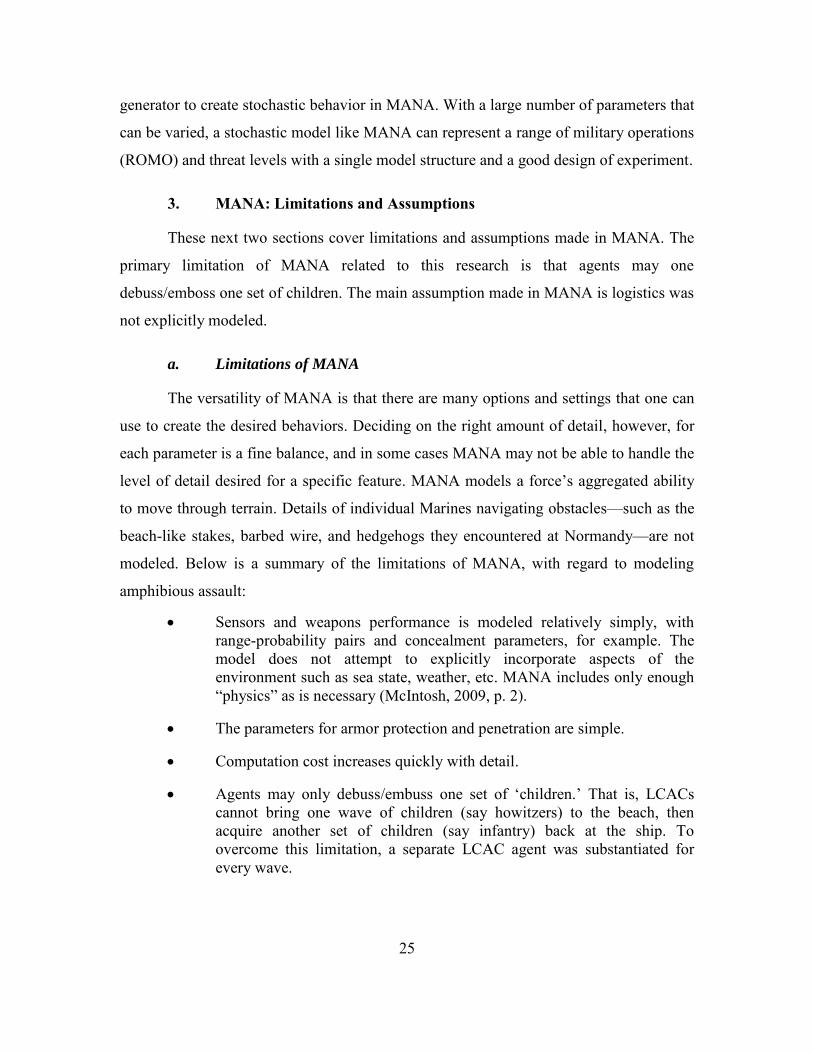
25

generator to create stochastic behavior in MANA. With a large number of parameters that

can be varied, a stochastic model like MANA can represent a range of military operations

(ROMO) and threat levels with a single model structure and a good design of experiment.

3. MANA: Limitations and Assumptions

These next two sections cover limitations and assumptions made in MANA. The

primary limitation of MANA related to this research is that agents may one

debuss/emboss one set of children. The main assumption made in MANA is logistics was

not explicitly modeled.

a. Limitations of MANA

The versatility of MANA is that there are many options and settings that one can

use to create the desired behaviors. Deciding on the right amount of detail, however, for

each parameter is a fine balance, and in some cases MANA may not be able to handle the

level of detail desired for a specific feature. MANA models a force’s aggregated ability

to move through terrain. Details of individual Marines navigating obstacles—such as the

beach-like stakes, barbed wire, and hedgehogs they encountered at Normandy—are not

modeled. Below is a summary of the limitations of MANA, with regard to modeling

amphibious assault:

Sensors and weapons performance is modeled relatively simply, with range-probability pairs and concealment parameters, for example. The model does not attempt to explicitly incorporate aspects of the environment such as sea state, weather, etc. MANA includes only enough “physics” as is necessary (McIntosh, 2009, p. 2).

The parameters for armor protection and penetration are simple.

Computation cost increases quickly with detail.

Agents may only debuss/embuss one set of ‘children.’ That is, LCACs cannot bring one wave of children (say howitzers) to the beach, then acquire another set of children (say infantry) back at the ship. To overcome this limitation, a separate LCAC agent was substantiated for every wave.

26

b. Assumptions Made in MANA

Other simplifications are made because the operational metamodels that results from

MANA excursions will eventually be linked with other software tools:

Fuel consumption—Fuel burn is not modeled in MANA. As seen in Chapter II, the USMC has VBA spreadsheet tools to calculate fuel burn.

Flight deck cycle—Deck cycle is not modeled in MANA. ACE is modeled via a DES in Simio.

Logistics—Resupply of fuel, ammunition, water, etc., is not modeled in MANA. Chapter II describes models that support logistical resupply.

Civilians—Neutrals or civilians also not modeled, as their impact to the MOP for different force configurations was deemed immaterial.

Beach conditions, sea state, weather, and elevation are not explicitly modeled.

C. RESEARCH QUESTIONS

This research shows the value of conducting large-scale design and analysis of

experiments with MANA. Meanwhile, since this research deals with specifications for

concept ACV and SSC, we seek to address the following questions:

What are the ACV MOPs that positively contribute to the MOEs?

What are the SSC MOPs that positively contribute to the MOEs?

Additionally, addressed in this section are EW 12 particulars which are applicable

to the operational scenario, and how those were implemented in MANA. We also provide

further details about the MANA implementation such as characteristics of the agents and

the playboard (simulated battlefield).

D. MEASURES OF EFFECTIVENESS

One purpose of the simulation in this research is to provide a tool to influence the

future development and procurement of the ACV and SSC. To do this we explore several

MOEs:

MOE (1): Blue casualties

MOE (2): Red casualties

27

MOE (3): Time to attrite the Red Force to 1/3 remaining strength

MOE (4): Force exchange ratio (FER), which is calculated for each run as (Red casualties +1) / (Blue casualties +1)

E. SCENARIOS

This research models a BLT-sized amphibious assault conducted four different

ways by a MEU while embarked on the ARG, as described in Chapter II. This section

presents the four scenarios modeled in this research. Subsequent sections present detailed

modeling particulars, as well as details on friendly and adversary agents in MANA.

1. Baseline Scenario (Scenario One)

This scenario is based on the adversaries FSM and WAF. Pockets of adversary

appear to be blending in with the local populace in the surrounding urban areas. A

moderate force is believed to be guarding against a likely amphibious assault operation;

however, they are unwilling to present overt defenses for fear of being targeted by CJTF

air strikes. There are groups of adversary inland, with few willing to risk exposure by

defending the coast. The enemy has 18 Red infantry, four Red medium/heavy artillery,

two Red tanks, and four Red anti-tank teams. The adversary has anticipated U.S.

involvement and believes that an urban avenue of approach is less likely than the landing

force seeking an envelopment of the city from the north. Enemy activity has been low so

an LCAC payload of ACV, M1A1, etc., unaccompanied on wave one is used to capitalize

on the shore-to-shore mobility and force protection afforded by the wheeled ACV. Figure

6 shows four LCAC SSCs returning to the seabase after wave one of bringing Blue forces

ashore.

28

Figure 6. Four LCACs or SSCs “+” returning to the seabase after bringing

Blue ashore.

2. Scenario Two

This scenario combines the baseline with AAVs. It is more likely than the

baseline scenario with LCACs operating alone. The MEU’s BLT will provide the landing

force for the ship-to-shore movement. As the LCACs bring waves of personnel and

equipment ashore, the CJTF employs self-deploying AAVs on wave one. The AAVs

remain in their approach lanes and accompany the LCACs on wave one, pressing inland

to establish security while friendly forces clear the landing beach. Once tactical integrity

and force consolidation are complete, the force continues with assault operations. Figure

7 shows four LCAC SSCs loaded with ACVs, M1A1 tanks, and equipment accompanied

by AAVs on wave one.

29

Figure 7. Four SSCs, capable of 4xACV or 1xM1A1 “LCAC loads.” The

MANA icon used for the LCAC is “+,” during a wave ashore, this icon will be overlayed by numerous icons of ACVs, M1A1 tanks,

and equipment. Wave one is accompanied by AAVs.

3. Scenario Three

This scenario combines the baseline with a MV-22 helicopter-borne raid inland.

Also known as STOM-V, this form of air assault with tilt rotor aircraft require an Area of

Responsibility (AoR) that does not have prohibitive air defense artillery (ADA) to rotary

wing operations. The CATF benefits from the deep insert afforded by tiltrotor aircraft,

which supports his overall scheme of maneuver (SOM). The CATF LCAC payload of

ACVs, M1A1s, etc., accompanied on wave one by tiltrotor aircraft, provide enhanced

littoral maneuver and a range of options for the landing force (Department of Defense,

1992). Figure 8 shows the heliborne raid of MV-22 aircraft from the seabase.

30

Figure 8. Heliborne raid of MV-22 aircraft from the seabase.

4. Scenario Four

This scenario combines AAV and MV-22 joint operations. The LCAC payload of

ACVs, M1A1s, etc., is accompanied on wave one by AAVs and MV-22s. In this STOM-

V and STOM-S amphibious assault the landing force (LF) takes advantage of additional

amphibian firepower and the range of tiltrotor insertion. The two forces then transition

from swimming and flying insertion forces to an on-land maneuver force (Department of

Defense, 1992). Figure 9 shows the combination of both a heliborne raid and AAV. The

necessary service craft deliver the ACVs, M1A1 tanks, and equipment ashore with an

accompaniment of AAVs on wave one.

31

Figure 9. Heliborne raid and wave one supported by AAVs.

F. MODELING PARTICULARS

In this section, we provide further details on how terrain was modeled, as well as

the force build-up ashore and the FLOT, all of which are vital to the CATF as discussed

in Chapter II.

1. Theater of War—The Sea, Surf, Shore, and Land

This MANA battlefield configuration has a global map size that is 70 nm by 70

nm. One time step in the model is equal to five seconds. Red and Blue agents on the

battlefield are organized into groups called “squads” and are limited by both terrain and

organic sensor capabilities, which together determine and what they can “see.” Maneuver

and placement of squads are relative to an X-Y Cartesian grid. An offshore area to the

southwest supports offshore distances of 25 nm.

Three types of maps form separate layers that make up the battlefield:

Background, Terrain, and Elevation. The background map is detailed imagery of the

theater of war, which is commonly satellite imagery of the AoR; it does not impact the

model computations, it simply serves as a background visual for the user. Meanwhile,

both the terrain and elevation maps do impact model calculations. MANA uses a

32

Windows bitmap file to define terrain, and each pixel is assigned distinct RGB (red,

green, and blue) color settings (McIntosh, Galligan, Anderson, & Lauren, 2007).

Additionally, each terrain type (color) is assigned a value of “going” (how well the pixel

can be traversed), “cover” (how much protection from fire the pixel provides), and

“concealment” (how much protection from sight the pixel provides); going, cover, and

concealment values range from 0.0 to 1.0. Figure 10 shows the RGB colors and going,

cover, and concealment properties for the terrain used in this scenario.

Figure 10. Terrain map, including the red, green, and blue (RGB) colors with

dark green shown at right.

In MANA, the scenario editor enables the design of custom terrain not present in

the defaults. An example of a default terrain is a road, which is colored with a particular

color of yellow. The terrain features used in the model are light brush, sand, heavy brush,

water, road, and building structure. Figure 10 shows that the road, which is colored with

(255, 255, 0) “yellow,” offers neither cover nor concealment, but perfect going.

Initial runs and variations were performed, and insights from these runs helped to

shape the baseline scenario. A killer-victim scoreboard Excel macro was used to explore

the results. These initial runs revealed the importance of massing combat power ashore

prior to assaulting through the objective. When squads arrived and continued to the

33

objective without waiting for the remaining components of the ATF, the lead elements

were destroyed. Initial replications also revealed the value of urban terrain. When the

terrain was turned off, the ATF was more vulnerable to the adversary’s artillery.

The ability to use “trigger states” in MANA is useful for specifying behaviors that

should occur when certain conditions were achieved. For example, in order to achieve

mass, agents in their default state release from their SSC and proceed to a predetermined

waypoint, and upon reaching that waypoint, their state changes to Reach Waypoint, and

in this state they wait until the rest of the force has landed ashore. Debarking agents from

SSCs continue to arrive, transition inland, and wait for the final wave of the ATF. This

reached waypoint state can be observed by the agent icon changing from its default blue

to pink. Once the final wave arrives, a symbolic ‘refueling’ interaction is performed,

which then triggers the entire landing force to move. Figure 11 shows the final wave

arriving, disembarking, and changing their state.

Figure 11. In order to mass force ashore prior to moving deeper into the threat

environment, agents must press inland and establish security (pink). Agents next await the final wave. As the final wave arrives squad 42, an agent representing CAAT, refuels friends, which cause the

advance (green).

34

2. Agents

In this section, we provide a summary of the different agent types used in MANA.

Table 1 provides an overview of all the agents created in MANA. From left to right it

shows the agent, description, their allegiance or side, agent class, and threat level. Agent

class and threat level can be used to specify sensor/weapon-target pairings.

Table 1. MANA Agent Classifications.

Agent Description of Blue Agent Allegiance Agent Class Threat

LHD Landing Helo dock, large air

capable ship 1 99 3

LPD Landing transport dock, L.

platform/dock 1 99 3 LSD Landing ship dock 1 99 3 LCAC Landing Craft, Air Cushion 1 88 3 AAV Assault Amphibious Vehicle 1 77 3 MV22 Medium lift, Tiltrotor aircraft 1 66 3 M1A1 Main battle Tank 1 2 3 LAVGrp Light Armored Vehicle 1 4 2 AntiTank CAAT or Anti-tank warfare team 1 5 2 BlueHowit Short barrel mobile artillery 1 3 2 Inf Four inf aggregated as a FT 1 1 1 ACV ACV, wheeled 1 4 3

Agent Description of Red Agent Allegiance Agent Class Threat

RedInfant Four Red inf aggregated as a FT 2 1 1 RedHowit Short barrel red mobile artillery 2 3 2 RedTanks Red Main battle Tank 2 2 3 RedAntiTank Red anti-tank warfare team 2 5 2

There are 113 squads in the scenario file that may be activated or deactivated.

Since a new squad assumes the squad number one higher than the last squad created, a

deleted squad changes the squad numbers of subsequent agents. Therefore, once a squad

is created it is helpful to keep it and just deactivate it in MANA so that squad numbers do

not change (if, for example, you would have to make many changes to documentation if

squad numbers changed).

35

a. Blue Agent Properties

Table 2 contains further details for some of the Blue agents. The table contains

squad numbers for individual tanks and ACVs, who their parent agent is, and the number

of agents in the squad. Table 2 also contains agent class number and a run start delay.

Run start delay is particularly useful when modeling agents that “come to life” and enter

the scenario at different times. For example, the delays before a second, third, or fourth

wave of LCACs launch. If an agent has a parent, then that agent is subject to its parent’s

run start. The parent of a tank or ACV represents the LCAC that carries that entity

ashore. More details are provided in Appendix A.

Table 2. This table shows the four M1A1 tanks and 19 ACVs modeled. The table also shows the LCAC squad number or parent agent that brings them

ashore. For example, ACV-P-1, ACV-P-2, & ACV-P-3 and the Recovery ACV (squad 93, ACV-R-1) all have the same parent.

Squad # Squad Parent # of Agents Agent Class # Run Start Delay 34 M1A1-1 4 1 2 0 35 M1A1-2 5 1 2 0 36 M1A1-3 7 1 2 0 37 M1A1-4 8 1 2 0 76 ACV-P-1 6 1 4 0 77 ACV-P-2 6 1 4 0 78 ACV-P-3 6 1 4 0 79 ACV-P-4 73 1 4 0 80 ACV-P-5 73 1 4 0 81 ACV-P-6 73 1 4 0 82 ACV-P-7 75 1 4 0 83 ACV-P-8 9 1 4 0 84 ACV-P-9 9 1 4 0 85 ACV-P-10 9 1 4 0 86 ACV-P-11 74 1 4 0 87 ACV-P-12 74 1 4 0 88 ACV-P-13 74 1 4 0 89 ACV-P-14 74 1 4 0 90 ACV-P-15 12 1 4 0 91 ACV-P-16 12 1 4 0 92 ACV-P-17 75 1 4 0 93 ACV-R-1 6 1 4 0 94 ACV-C-1 73 1 4 0

36

Blue agents all have allegiance “1.” Table 2 shows a run start delay of zero for all

of the squads listed here, because they are the children of LCAC agents. The agent class

number allows entities to target and be targeted by appropriate types of agents. For

example, infantry will target other infantry and CAAT, while CAAT will target both

infantry and tanks.

Placement of Red agents was in accordance with the EW 12 scenario. At the

beginning of the simulation, the Blue agents are all located at the seabase. The operations

from the MLP or seabase debuss SSCs, which then debuss ACVs by waves that swim to

the shore. Later, at the objective, the ACV debusses its Blue infantry. Once Red classifies

Blue targets, the Red forces engage.

The subsequent sections provide additional detail regarding modeling of:

Seabase

SSC

AAV (self-deployer)

MV-22

ACV (shore-to-shore variant)

M1A1

CAAT

Howitzers

Infantry

(1) Seabase

The ARG is the seabase modeled in this research. While the ARG is smaller than

the ESG, these three ships are indicative of the capability sailing at any given point

within the three operational MEUs. The model can easily be adapted to other forms of

seabases since there are many options for the seabase. In many of the likely scenarios, the

seabase is OTH, postured to support low signature SSC to deploy APCs, ACVs, and

AAVs close to shore during one period of darkness. The modeled three vessels that

comprise the ARG seabase have the properties discussed in Chapter II. The basic model

37

structure can be modified to incorporate MLP, which can bring more LCACs and the

JHSV capable of offloading ACV offshore. The JHSV and MLP programs advertise

increased maneuverability and speed. Figure 12 shows the LHD agent. Figure 12 depicts

the MANA graphical user interface (GUI) screen for setting agent “personality,” and

shows that the LHD in its default state has a personality weight of 50 toward its next

waypoint. Note that all other personality weightings have been assigned a value of 0,

ensuring that while in this state the LHD will only move towards its next waypoint and

will not engage in other behaviors.

Figure 12. LHD Agent: Depicts the GUI for in MANA. The agent icon is

located in the lower left, possible trigger states (e.g., Default State, Reach Final Waypoint) are in a column to the right.

(2) Ship-to-Shore Connectors

We chose to model the LCAC SSC because the service life extension program for

the LCAC will continue its use through 2027, and it represents the current ARG

capability. Furthermore, since LCACs presently serve as the Navy’s high speed

connectors, they represent a worst case. An operation requiring multiple waves also

represents a worst case. It is feasible that a JHSV or UHAC loaded with ACV could

38

deploy a much higher volume of ACV, but that was not a focus of this research. This

research took care to model a more limited and yet practical scenario with three waves of,

at most, four LCACs. If a JHSV or MLP is desired, an arrival of ACV at a certain time

and location offshore is easier to model in MANA than what might be required to make a

similar change in a coded model (e.g., VBA). Nevertheless, an LCAC can carry

approximately 120,000 lbs at speeds of 40 kts in seas with waves heights of 4.1 to 8.2

feet, averaging 6.2 feet (Department of the Navy, 2007). Figure 13 shows the three

LCAC waves from the ARG. A total of four LCACs are selected, based on the new LHA

and LPD configurations.

Figure 13. Baseline factor of four LCACs as the SSC. The bottom right square

shows the fourth LCAC on the first wave loaded with four ACV. The squad number is 73 for that particular LCAC. One may alter the design features of these “black box LCAC” to upgrade this modeled

agent capability to JHSV, UHAC, “Mike Boats” (LCM-8), LCU, concept LCAC, etc.

Figure 13 also represents the future for this research. The “black box LCAC” can

be configured to represent any possible future SSC. Modeled LCACs have the Run Start

39

trigger state enabled. The Run Start time includes a delay for loading and offloading

vehicles and equipment. For each wave, a new set of LCAC agents are used. Chapter II

described one benefit of amphibious ops is the attacker’s ability to determine the time and

place. Modeling waves with run start delays is reasonable, as the mission is time-driven.

Figure 14 shows a negative weighting towards friendlies, and the negative weight results

in squads that are more dispersed on the battlefield (McIntosh, Galligan, Anderson, &

Lauren, 2007). Figure 14 also shows the Run Start trigger state in the far right column

(font shaded green).

Figure 14. LCAC Agent: Depicts the Personalities GUI in MANA. The agent

icon is located in the lower left, possible trigger states (e.g., Default State, Reach Waypoint, Reach Final Waypoint, Run Start) have a

check in the box. The Run Start trigger state is unique to the LCAC, as their waves are based on time.

(3) Amphibious Assault Vehicles

The legacy AAV still deploys regularly with the MEU. Therefore, excursions

using the BLT and AAVs are likely as ACVs are meant to serve as reinforcing echelons

of a JFEO. Assuming that an MEU-sized force (BLT) would be first ashore; a question

this research sought to answer was how the ACV as a shore-to-shore increment could be

40

more effective than the old AAV or previous increment. Nine AAVs were modeled for

wave one, which was based on the number required for a company of lift. Shore-to-shore

and ship-to-shore mobility were covered in Chapter II and represent the future life cycle

of the ACV. The AAV was modeled to hold a reinforced infantry squad.

The weapon for the AAV was modeled to represent a 0.50 cal machine gun.

Speeds for the AAV ranged from swim speeds of eight knots to land speeds of 40 mph. A

remote weapon station (RWS) was not considered, however, it could be implemented

based on the considerations outlined for the ACV and upgrades intended for this 40 year-

old platform. The GUI in MANA for the AAV differs from the LCAC (Figure 14) only in

that the agent icon located in the lower left is a Blue tracked APC. Possible trigger states

(e.g., Default State, Reach Waypoint, Reach Final Waypoint, Run Start) remain the same

as for the LCAC. This section covers the agent used to model an amphibian self-

deploying vehicle comparable to the AAV. However, it is also well suited to model the

EFV, ACV 2.0 increment as TRL improves.

(4) MV-22

STOM-V provides rapid inland ranging and additional Marine FT lift capability,

as required of scenario 3. The GUI in MANA for the MV-22 differs from the LCAC

(Figure 14) only in that the agent icon located in the lower left is a Blue helicopter and

dispersion is affected by a personality weight of –30 from other friends. The MV-22 has a

7.62 millimeter (mm) gun aircraft unit and several crew served weapon systems. These

options, such as a tail gunner, limit the altitudes at which they can fly. Modeled instead

are the embussing behavior of 24 combated-loaded Marines on each MV-22. The speed,

vulnerability, and range of the MV-22 are modeled—weapons and the deck cycle are not.

(5) Amphibious Combat Vehicles

Nineteen ACVs are modeled in this research: 17 normal ACVs (ACV-P[1-17]), a

repair or towing variant, and communications variant. The ACV is the main Marine

carrier or vehicle for this research. Two ACV can carry a reinforced Marine rifle squad

and two days of supply. Since there are two ACV for what was one AAV, the ACV

brings two RWS. The ACV may also be configured with a MK-19 grenade launcher,

41

which is not modeled, however, the RWS and increased armor is modeled—as compared

to the legacy AAV. There are three crew members: the vehicle commander, a gunner, and

a driver. A Marine company of lift requires 21 ACV. Two to four FTs per ACV cover the

requirement that 10 to 15 Marines be onboard (8-16 Marines were modeled). The speed

of the ACV allows it to keep up with the M1A1. The questions surrounding the ACV are

ideal to explore with MANA. For example, armor, increased lethality in the RWS, and

cross country speeds comparable with the M1A1 in A2/AD or degraded mobility, are all

parameters that can be changed in MANA. Similarly, MANA supports the

interoperability with connectors too. As mentioned previously, L-Class ships (e.g., LHD,

LPD, etc.,) and MPF bring additional SSCs.

Four trigger states were implemented in MANA to incorporate the complexity of

amphibious operations. First, the Default State covers the swim from debussing from the

LCAC to a safe location ashore at distances of 5, 12, 25 nautical miles (nm). Second,

Reach Waypoint stops the ACV from advancing inland. Instead they establish security,

awaiting the complete force buildup. Third, as previously described, Refueled By Friend

occurs once the final wave arrives (because a member of that wave refuels friendlies).

Fourth, Reach Final Waypoint dismounts infantry on or near the objective, upon reaching

the final waypoint. Figure 15 shows the four trigger states that are active for all the

ACVs. It also shows the agent icon, which is also that of the AAV.

42

Figure 15. ACV agent: Depicts the GUI for in MANA. Trigger states used are

the Default State, Reach Waypoint, Refuel By Friend, and Reach Final Waypoint. Run start is not required as the ACV are debussed

from LCAC when the LCAC reaches its debark point.

The next few screen shots show the ACV squad properties:

Tangibles tab: Shows movement speeds, threat, allegiance, and agent class information.

Sensors tab: Provides probabilistic detection and classification range information and target class prioritization.

Weapons tab: Shows round counts, reload time, maximum effective ranges, penetration, and probability of hit.

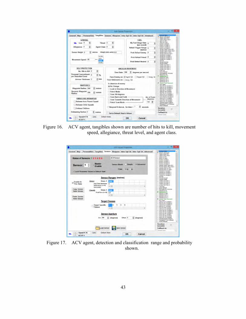
43

Figure 16. ACV agent, tangibles shown are number of hits to kill, movement

speed, allegiance, threat level, and agent class.

Figure 17. ACV agent, detection and classification range and probability

shown.

44

Figure 18. ACV agent, depicts weapon ranges, probability of hit, round count,

reload time, target priority list.

(6) M1A1 Abrams Tank

The LF has four main battle tanks embarked on the MEU. LCAC modeled are

only capable of waves of a single tank. The tank provides superior firepower and

mobility. The tank, too, has gone through several series and upgrades. This thesis does

not focus on this type of vehicle, save for the fact that many amphibious requirements are

being based on keeping up with the M1A1’s cross-country speed of approximately 45

mph. The M1A1 also has excellent armor. For modeling purposes, the tank’s armor and

number of hits required to kill it, represent an upper bound for all agents. Yet, even the

M1A1 is limited by target acquisition, that is, the ability to classify an enemy. One thing

to keep in mind is that the tank’s 120 mm round has a higher logistical footprint, as

compared to other ammunition, like that of the 0.50 cal. Therefore, if further excursions

are run in MANA, the user may want to consider how to capture the additional logistical

strain associated with longer battles and or increased battle intensity.

45

(7) Combined Anti-Armor Team

The CAAT is unique in that it both has a personality weight to move toward an

ideal enemy, and that it refuels friendly agents when it arrives last, for reasons previously

described in Section C of this chapter (Figure 11). Figure 19 shows a positive personality

weight to target its “ideal class,” Red tanks (which are agent class 2). This ensures that

the CAAT will engage enemy armor units whenever possible. The modeled weapon is

comparable with a tube-launched optically tracked, wire-guided (TOW) missile system.

Modeling the TOW missile system provides a lower bound worst case as there are other

tank missile systems (e.g., AGM-114, Spike, Javelin) that have higher probability of

weapons release, probability of hit, and probability of damage given a hit, than the TOW.

The CAAT have three rounds, with a delay in between attempts, but with good armor

penetration.

Figure 19. CAAT agent called AntiTankTm1, represented in pink, has a

personality weight to move toward Red tanks. Once released from emboss, the agent seeks to Refuel Friends (see: Section C of this

chapter).

46

(8) Howitzers

Howitzers are not known for their mobility. The agent name preserves the

purpose of this agent—long to medium range artillery. The expeditionary fire support

system (EFSS) provides expeditionary fire support. While the right mix of mobile to

fixed artillery is not the focus of the research, expeditionary artillery is part of the future

concepts decision makers will be considering for EF-21. The structure of the model is not

currently equipped to explore the impacts of the CH-53K requirement to be able to

externally load the EFSS and its vehicle. However, this model can demonstrate the

impacts of mobile artillery fire.

(9) Infantry

Infantry are loaded aboard the AAV, ACV, and MV-22. In MANA, all of the

embussed infantry are secure in their APC until the infantry are debussed or dropped off

at either the landing zone or the objective. That is because, in this model, there is no

hostile resistance against the carriers. This could be changed in the future, if desired.

Several methods can be employed to release infantry from their parent. The method used

here is that the infantry are released upon the carrier reaching its objective. Dismounting

infantry earlier exposes them to enemy fire, while dismounting later runs the risk of

increased casualties if the entire vehicle is destroyed (e.g., from IED, artillery, etc.). A

method of maintaining mass with the infantry is to preserve the FLOT until reaching the

objective. Multiple waves in an amphibious assault and terrain make formulating a FLOT

challenging. Terrain includes the surf, sand, and urban terrain from streets and structures.

The AAV can hold a reinforced rifle sqaud. The ACV will hold less than a

complete squad of Marines. A squad is 13 Marines, comprised of a squad leader and

three FT of four Marines each. The FT concept is unique to the USMC and is designed to

bring increased firepower on the enemy. Some argue that a weakness of the ACV is that

it potentially splits up FTs and the squad between two vehicles. Since 2007, however,

Marines have ridden in combat in a vehicle that holds a payload comparable to the ACV,

specifically the Mine-Resistant Ambush Protected (MRAP) vehicle. APCs designed to

withstand IEDs were vital for OIF and OEF. As seen in Chapter II, Marines anticipate

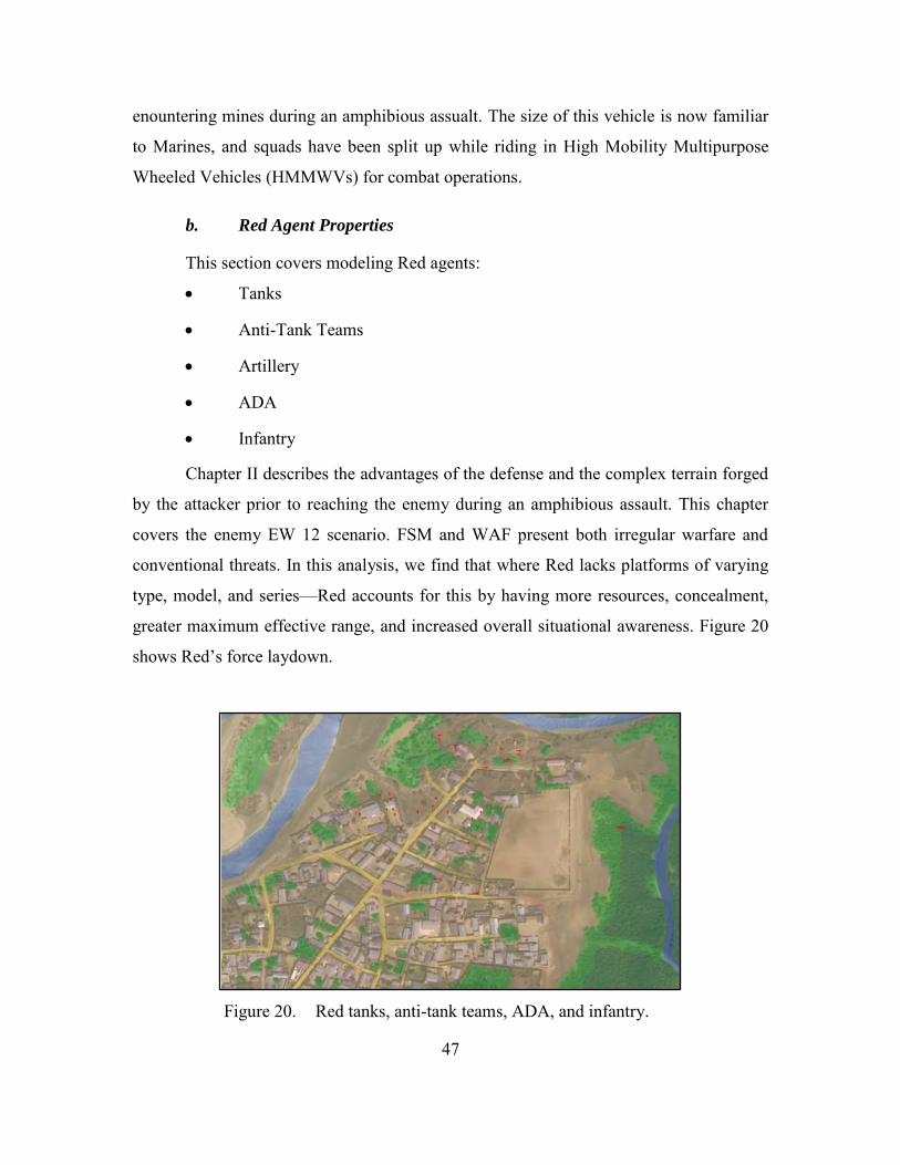
47

enountering mines during an amphibious assualt. The size of this vehicle is now familiar

to Marines, and squads have been split up while riding in High Mobility Multipurpose

Wheeled Vehicles (HMMWVs) for combat operations.

b. Red Agent Properties

This section covers modeling Red agents:

Tanks

Anti-Tank Teams

Artillery

ADA

Infantry

Chapter II describes the advantages of the defense and the complex terrain forged

by the attacker prior to reaching the enemy during an amphibious assault. This chapter

covers the enemy EW 12 scenario. FSM and WAF present both irregular warfare and

conventional threats. In this analysis, we find that where Red lacks platforms of varying

type, model, and series—Red accounts for this by having more resources, concealment,

greater maximum effective range, and increased overall situational awareness. Figure 20

shows Red’s force laydown.

Figure 20. Red tanks, anti-tank teams, ADA, and infantry.

48

(1) Red Tank

There are two heavily armored and concealed tanks for Red. Both tanks have

sensors that out-range Blue tanks by 1,000 meters (m). Red tanks also have better

logistics; therefore, Red tanks enjoy higher round counts than Blue. Red tanks only have

one state and move so as to avoid being decisively engaged. Red tanks are superior to

Blue tanks to give the advantage to the defense and make it formidable.

(2) Red Anti-Tank Team

There are two well-trained anti-tank teams. These teams also enjoy better

concealment and logistics than Blue. The anti-tank team has personal concealment per

detection event equal to 50%, which means it has a 50% chance of not being acquired by

Blue. For reference, a concealment value of 100% will give a Red anti-tank team agent a

0% chance of being seen (McIntosh, Galligan, Anderson, & Lauren, 2007).

(3) Red Artillery, Air Defense Artillery

The Red artillery has personal concealment per detection event equal to 70%,

given the FSM’s ability to blend in with the local populace, or the WAF’s proclivity to

nest their artillery near cities or in other areas that make targeting difficult. Red artillery

also models the impact of air defense artillery, as Red artillery actually prioritizes Red

aircraft above infantry and CAAT.

(4) Red Infantry

Red infantry enjoy some of the similar befits of the defense and basic

characteristics of the scenario described. Like Red artillery, Red infantry are all 70%

concealed. The Red force is massed or concentrated, which creates a formidable defense

for Blue. Red is also organized with a layered defense, ranging Blue as they advance

toward Red’s position. In MANA, every Red infantry requires 11 hits to be killed,

meaning Red infantry is 11 times harder to kill than Blue. The number 11 is somewhat

arbitrary, but served to provide a reasonable Killer-Victim scoreboard baseline.

49

IV. DESIGN OF EXPERIMENTS

This chapter covers the design of experiment; specifically, the choice of factors

and levels, robust design, and design choice. Additionally, we discuss how the number of

replications was determined, as well as how the experiment was executed.


Understanding the fundamentals of DOE is important. Without an adequate

understanding, the experimenter risks wasting time and resources, and unnecessarily

limiting the analysis that can be performed on the data. Our DOE considers four scenario

types and 77 other factors. From the seabase, force masses ashore via one of the

following configurations: Figure 21 shows the baseline scenario, scenario 1, is

highlighted in white, with its major components listed in the schematic.

LCAC (ACV)

LCAC (ACV) + AAV

LCAC (ACV) + MV-22

LCAC (ACV) + AAV + MV-22

Figure 21. Experiment setup schematic, which shows the four scenarios and

two other decision factors: (1) distance from shore that ACVs are deployed from the SSCs, and (2) the number of SSCs.

50

Figure 21 summarizes the four scenario alternatives. The bottom left corner of

Figure 21 shows the seabase. The baseline/scenario 1 consists of LCACs completing no

more than four waves, bringing ashore 17 ACVs, four M1A1s, and the supporting

equipment. These waves are unaccompanied by legacy AAV or MV-22 support.

Scenarios two and three build on this, bringing additional forces ashore either from

STOM-S or STOM-V. The factor settings listed at the bottom of Figure 21 show that the

ACVs may be launched to swim to shore from 5, 12, or 25 nm, and that 2, 3, or 4 LCACs

are used to transport the ACVs.

To build our efficient DOE for a MANA model, we conduct the following steps:

1. Define decision and noise factors, and their levels/bounds 2. Select the appropriate design 3. Verify the design, ensuring space-filling and low correlation properties

1. Factors and Ranges of Interest

Factors of interest cover a broad range of possible parameters; inputs that were

developed in both Chapters II and III. Factors can be either continuous or

discrete/categorical. Tables 3 and 4 contain complete listings of all Blue and red factors,

respectively. Both Table 3 and 4 show factors other than the scenario type, a brief

description, their minimum (Min), current, and maximum (Max) values (if continuous)

and their levels (if discrete or categorical). The following tables are colored red and blue,

which is used to distinguish threat (if Red) and friendly (if Blue). Various data in the two

Min and Max columns are highlighted in yellow to break out the continuous variables

from the categorical. Since we can adjust these variables they are controllable factors,

which will be explained in greater detail after the table.

51

Table 3. Complete listing of Blue experiment factors.

BLUE Agent Explanation Factor Min Max Current Unit

- Amphib debark distance LCDbkDist 5 25 12 run ... :E "' Amphib velocity LCl\MSpd 10 30 25 kts u Velocitv at Default State LCACMvtSpd 25 60 42 kts ~ )lo. Hits to kill LCACHit2k I 3 I Hits u ....l )lumber of LCACs deployed in Amphibious Readv Group LCACQty 2 4 4 LCAC

Sensor Deteclion Range at Default State AA VSnrDetRng 8000 10000 5000 meter Sensor Classification Range at Default State AA VSnrC!sRng 1000 8000 3000 meter

> Swimming Velocitv at Default State in the water AAVMvtSpd 5 42 34 kts ~ )lo. Hits to kill AAVHit2k I 3 I Hits ~

Remote Weapon Station (RWS) Range AAVrws 800 2000 1000 meter InfantrY carrving capacitv AAVInfCap 2 4 4 infantrY Sensor Detection Range at Default State ACVSnrDetRng 8000 10000 5000 meter Sensor Classification Range at Default State ACVSnrC!sRng 1000 8000 3000 meter

G Sensor Classification Range at Default State, Probability ACVSnrC!sProb 0.5 0.95 0.7 Swimming Velocitv at Default State in the water ACVMvtSpd 8 45 40 mph

~ )lo. Hits to kill ACVHit2k I 3 2 Hits Remote Weapon Station (RWS) Range AAVrws 800 2000 1000 meter InfantrY carrving capacitv ACVInfCap 2 4 10 infantrY Sensor Detection Range at Default State 1\·fVSnrDetRng 8000 10000 5000 meter

"' Sensor Classification Range at Default State MVSnrC!sRng 1000 8000 3000 meter

"' Sensor Classification Range at Default State, Probabilitv 1\·fVSnrC!sProb 0.5 0.95 0.7

~ Velocitv at Default State 1\·fVMvtSpd 90 220 100 mph )lo. Hits to kill l\·fVHit2k I 3 2 Hits InfantrY carrving capacity 1\·fVInfCap 5 7 6 Infan!rj Sensor Detection Range at Default State M!SnrDetRng 8000 10000 6000 meter Sensor Classification Range at Default State M I SnrC!sRng 2500 8000 5000 meter ... WeaPOn. max effective range M!WeapRng 1500 8000 3500 meter

~ WeaPOn. ran~te probabilitv M!WeapProb 0.4 0.93 0.4 ... ~ Sensor Classification Range at Default State, Probabilitv M I SnrC!sProb 0.4 0.95 0.95

Velocitv at Default State M!MvtSpd 30 50 40 mph )lo. Hits to kill M!Hit2k 2 4 3 Hits Sensor Detection Range at Default State AntTnkSnrDetRng 8500 10000 8000 meter

.:.= Sensor Classification Range at Default State AntTnkSnrC!sRng 1000 8500 7000 meter 1: Sensor Classification Range at Default State. Probability AntTnkSnrC!sProb 0.5 0.95 0.9 ~

AntTnkMvtSpd !- Velocitv at Default State 3 40 25 mph :.c c )lo. Hits to kill AntTnkHit2k I 2 I Hits ~

WeaPOn. max effective range AntTnkWeapRng 1000 8000 4000 meter WeaPOn. ran~te probabilitv AntTnkWeapProb 0.4 0.8 0.4 Sensor Detection Range at Default State HowitSnrDetRng 15000 19000 12000 meter .. Sensor Classification Range at Default State HowitSnrC!sRng 10000 15000 11000 meter .. Sensor Classification Range at Default State, Probability HowitSnrC!sProb 0.5 0.95 0.8 ll

'i Velocitv at Default State Howiti\MSpd 3 40 40 mph ..2 )lo. Hits to kill HowitHit2k I 3 3 Hits - WeaPOn. effective casualtv radius range HowitWeapRadRng 15 30 15 meter

WeaPOn. ran~te probabilitv HowitWeapRadProb 0.5 0.95 0.75

.... Sensor Detection Range at Default State InfSnrDetRng 3000 5000 3000 meter b Sensor Classification Range at Default State InfSnrC!sRng I 3000 3000 meter c

Sensor Classification Range at Default State. Probabilitv InfSnrCisProb 0.5 0.9 0.6 .! .: Velocitv at Default State InfMvtSpd 2 4 3 km!hr )lo. Hits to kill InfHit2k I 4 I Hits

52

Table 4. Complete listing of Red experiment factors.

a. Controllable Factors

Factors in a design are classified as controllable if they can be controlled in the

real world. Factors are uncontrollable if they are outside of the operator’s control. There

are many controllable factors associated with an amphibious assault. Operators may

select from a variety of platforms. Additionally, the numbers of ACVs, SSCs, and

helicopters are all controllable factors. It should be noted that some factors in a design

may require changes to the structure of the simulation, and we use a translation to handle

mappings and dependencies. For example, Figure 22 is a schematic that shows how the

simulation’s landing plan was adjusted to accommodate different numbers of LCACs.

53

Figure 22. A schematic of how the simulation’s landing plan was adjusted to

accommodate 2, 3, and 4 LCACs.

b. Uncontrollable Factors

In contrast to controllable factors, uncontrollable (or “noise”) factors are those

that operators cannot control in the real world. In an amphibious assault, noise factors

included wave height, wind velocity, and terrain. All of the rows colored in red in Table 3

represent uncontrollable factors. Noise factors are important to consider when providing a

robust solution that will work in many different situations. Often, scenario-based analysis

becomes too dependent upon hordes of unrealistic assumptions. While this research

leverages EW 12, it is important to provide a broad analysis that considers a range of

noise factors, in order to generate a robust solution. Moreover, while waves, winds, and

weather are important for a higher-resolution study of the physical environment, the noise

factors in our experiment are associated with characteristics of the threat. With the threat

factors, we cover a broad range of possibilities for how well the enemy can sense and

prosecute the incoming Blue forces with firepower.

54

c. Robust Design

Building the ACVs and SSCs will take time and cost a lot of money. The time and

cost associated with running simulation experiments is much less than making changes

on the real system, and can incorporate changes more quickly than upgrading the ACV.

The robust design approach was forged by Toyota engineer and statistician Genichi

Taguchi (1986). In the simulation context, the simulation is a surrogate for the real

system, which may realize the benefits of improved performance and decreased cost

faster than the manufactured system (Sanchez, 1994). With all the factors, inputs, and

alternatives for a given system, we proceed with a design process akin to simulation

optimization, where the “best” answer is not overly sensitive to small changes in the

system’s inputs (Sanchez, 1994). Procured future equipment of the Navy and Marine

Corps should be robust to a variety of missions and threats based on the approach above.

Today, the adaptive adversary will change based upon technology; therefore, technology

must be flexible enough to perform a variety of things well.

B. NEARLY ORTHOGONAL AND BALANCED (NOB) MIXED DESIGNS

In this research, 78 factors, including scenario type, were varied over several

hundreds of thousands of simulated amphibious assaults. Here, we take a step back and

discuss how efficiency, which is the number of design points required to study k factors

with m levels each, can vary considerably across possible design types. For example, to

study four factors with two levels each, using a full-factorial design that investigates

every possible combination, would require 24=16 design points. A full factorial design of

four factors with four levels each would require 44=256 design points. Increasing the

number of factors and/or levels for a full factorial design causes the number of design

points needed to increase exponentially, and this is referred to as the “curse of

dimensionality.” A much more efficient design, developed at the Naval Postgraduate

School, is called the Nearly-Orthogonal Latin Hypercube (NOLH). NOLH designs have

good space-filling and orthogonality properties (Sanchez, Sanchez, & Wan, 2014).

Figures 23c and 23d show a good example of the difference in coverage between factorial

55

and NOLH designs. Figure 23 shows a comparison of the pairwise projection plots for

two factorial (if top row) and two NOLH designs (if bottom row).

Figure 23. The top row features factorial designs and the bottom row illustrates

the near-orthogonality and space-filling properties of NOLH designs (from Sanchez, Sanchez, & Wan, 2014).

The computational savings of the NOLH designs is enormous; but, the NOLH

design is best suited for continuous factors. The inclusion of discrete or categorical

factors can cause the pairwise correlations to increase, due to the rounding involved.

Therefore, since our design contains several discrete factors, we use one of the new

designs—the nearly orthogonal-and-balanced (NOB) mixed designs of Vieira, Jr.,

56

Sanchez, Kienitz, and Belderrain (2011, 2012). For this research, the 512-design point,

NOB design template, available at http://harvest.nps.edu, is used. Figure 24 contains an

excerpt of the 512-design point, NOB design spreadsheet template. Additionally, the low

and high values we see in this figure are the same as the maximum and minimum values

we saw in Table 3.

Figure 24. An excerpt of the 512-design point, NOB design spreadsheet

template, which allows for the investigation of the 77 factors. The template can handle simultaneous investigation of 300 factors, with

discrete number levels and continuous-valued factors (after Sanchez, Sanchez, & Wan, 2014).

As previously mentioned, not only are these designs space-filling, but they also

produce the near-orthogonality desired for regression analysis. All pairwise correlations

are less than 0.012 in our design. A color map of correlations can be used to visualize

pairwise correlations, and is shown in Figure 25. The 77 red cubes connected along the

57

diagonal depict the perfect positive correlation (i.e., red = 1.0) between the factor and

itself, while the remaining area is shaded grey, which shows a near-zero correlation

between any factors that are not the same. Appendix G shows a multivariate plot for the

complete design.

Figure 25. Color map of the design’s pairwise correlations.

C. EXECUTING THE EXPERIMENT

The NOB design spreadsheet provides 512 design points for the 77 factors (not

including the scenario type). The design for the 77 factors was then crossed with the

scenario type factor, yielding a total of 4 512 2,048 design points. EW 12, MEB

concept of operations, and research covered in Chapters I and II were used to guide the

selection of factors, ranges, and levels. For example, E2O provided many of the ranges

for factors covered, as these values were deemed interesting to the stakeholder, based on

key performance parameters and objective threshold values for systems being procured.

Each design point was run using 30 different random seeds. We discuss the rationale for

using 30 replications in Section D.

The following section describes how the Simulation Experiments and Efficient

Designs (SEED) Center configured and executed the DOE. The base case MANA

scenario, in eXtensible Markup Language (XML) format, and the DOE file, in comma-

58

separated value (CSV) format, were entered into a software program called XStudy,

written by SEED Center Research Associate Steve Upton. XStudy enables the user to

map each column in the design file to a specific parameter element in MANA, using

XPaths. An XPath is a reference to a specific location in an xml file. Other details about

the study design, such as the version of MANA and the number of replications per design

point, are also entered into this tool, yielding a single “study.xml” file. This study file is

used by another program called oldmcdata, also written by SEED Center Research

Associate Steve Upton, which programmatically modifies the MANA XML file,

producing a separate XML scenario file for each design point. An open source software

package called condor, available from the University of Wisconsin

(http://www.cs.wisc.edu/condor), is used to distribute and manage the MANA jobs in

parallel across a set of available processors. The oldmcdata software creates the set of

submit.dat files needed by condor, one for each design point job. A job consists of a set

of replications for one design point excursion. Upon completion of the runs, oldmcdata

includes a data postprocessor that combines MANA summary file output from the

individual design point excursions into one csv file, ready for use with any data analysis

software package. This output file contains input factor settings from the DOE, the

random number seed, and outputs for each replication. The SEED Center high-

performance computing cluster configuration used for these runs was composed of 128

Windows processors, with 2-4 gigabytes (GB) of random-access (RAM) per processor.

D. NUMBER OF REPLICATIONS

One replication of the base case MANA takes, on average, 10 minutes, and this

computational cost must be taken into account when determining how many replications to

perform. One method for determining an adequate number of replications is the data given in

Equation 1. We will use this equation to estimate the sample size needed to perform null

hypothesis significance testing given the Blue casualties’ MOE. Our choice for alpha ,

which represents Type I error, was 0.05. The choice for power, which is 1 minus beta , the

Type II error, was 0.95. In Equation 1, then, αZ 1.96 and Z 1.64 . Our choice for the

59

practical difference we want to detect, in the denominator, was 2, and the estimate for standard

deviation, based on 100 replications of the base case, was 5.86.

2

α β

0

σ Z Zn

μ μ'

(1)

The resulting sample size n , given our values described above, is 112. The cost

in computational power and time, however, might not support doing this many

replications. We note that we could lower n to 68 by dropping power to 0.8 (a common

choice), vice 0.95. We turn next to visualizing, in Figure 27, how the half-width of the

confidence interval for the mean decreases as a function of the number of replications, in

order to determine where diminishing returns occur. As the confidence interval half-

width decreases, we achieve increased precision on our estimate of the mean. Figure 27

shows that while 112 samples might be ideal, the additional precision acquired by doing

between 30 and 100 replications may not be worth the increased computation cost. This

is particularly true because when we fit metamodels to the resulting output, we are able to

leverage data collected from the entire design to estimate factor effects. This substantially

increases the power of the statistical tests.

Figure 26. Confidence interval half-width diminishing returns, based on the

number of replications. It appears that the added benefit from going from 30 replications to 100 might not be worth the computational

cost of running a MANA simulation that takes 10 minutes, on average, for each simulation.

60

In the end, we choose to perform 30 replications of each of our 2,048 design

points, resulting in 61,440 total simulation runs. Given access to the SEED Center’s 128

Windows processors with 2-4 GB of RAM each, we are able to complete the experiment

in approximately 3.5 days.

61

V. DISTRIBUTED FLIGHT DECK OPERATIONS AND SIMIO MODEL DEVELOPMENT

This chapter begins with a general overview of the deck cycle for aircraft on an

amphibious ship, such as an LHD, and the selected DES modeling software, Simio.

Additionally, it covers the benefits and limitations of Simio, which includes why DES is

also useful to DOD decision makers. Finally, we will review the research questions for

this first-stage model and describe the Simio modeling. This Simio model is an example

of what Cioppa, Lucas, and Sanchez (2004) describe as a model that attempts to capture

“the salient features of the situation without trying to model all of the details that could be

considered” (Cioppa, Lucas, & Sanchez, 2004, p. 172).


The principle finding of “Operational Energy/Operational Effectiveness (OE2)

Investigation for Scalable Marine Expeditionary Brigade Forces in Contingency

Response Scenarios” is that operational energy consumed from QRF and MEDEVAC air

platforms launched from the seabase are the primary drivers of energy during

expeditionary operations. Seabased aviation operations consume energy over both

workups and the deployment of a MEU. The MEU regularly launches ACE platforms in

support of a ROMO, including VBSS, HA/DR, A2/AD, etc. The launch and recovery of

aircraft from the ARG is called the “deck cycle.” Groupings of aircraft that launch

together for a mission are commonly called “packages.” In order to better understand the

impacts to operational energy for a BLT force ashore, we will construct a first-stage

model of a nominal air raid package required for the insertion of the screening force

described in Chapter II.

The MEU’s ACE consists of a parent MV-22 squadron reinforced with several

detachments of light attack, strike, and heavy-lift aircraft from other redeployed units.

Typically, the ACE consists of 12 MV-22s, 4 AH-1Zs, 2 UH-1Ys, 6 F-35Bs, and

4 CH-53Ks. The MEU commander may retain the ACE on the LHD or allocate aircraft to

other air-capable ships (i.e., place aircraft on LPDs) during split or disaggregated

62

operations. These operations require coordination via a detailed flight schedule. A flight

schedule is produced daily that includes both the Marine aircraft from the ACE and the

Navy’s search and rescue (SAR) platform, the SH-60. The flight schedule establishes

when the ships will conduct flight operations (“flight quarters”) and deconflict launch and

recovery times of aircraft from spots. The only aircraft that requires the use of the entire

deck for take-off (“deck-run”) is the F-35B. Aircraft are kept on the forward and aft

“slash” areas prior to being towed out to a spot for launch. A launch, like the MV-22 seen

taking off in Figure 27 has a sequence of steps leading up to the actual launch:

1. Aircraft spotted – Aircraft towed from slash to spot. 2. “Chocks and chains” – Aircraft secured to the flight deck spot

(i.e., chocks and chains put in place). 3. Aircraft are loaded with the mission fuel and ordnance. 4. Startup. 5. “Breakdown” – Aircraft chains and chocks are removed. 6. Arming – Ordnance crews and/or crew chiefs remove safety mechanisms

from weapons and survival systems. 7. Launch – Deck crews clear the aircraft for subsequent takeoff.

Figure 27. Figure 28 shows an MV-22 Osprey launching from a forward spot.

All three aircraft, to include the CH-53E, belong to Marine Medium Tiltrotor Squadron (VMM) 265 (Reinforced)

(from Achterling, 2014).

63

Three aircraft are shown, two MV-22s—one of which is taking off—and a

CH-53. The aircraft are assigned to Marine Medium Tiltrotor Squadron (VMM) 265

(Reinforced) aboard the USS Bonhomme Richard (LHD 6) (Achterling, 2014).

Figure 28 shows two groupings of MV-22 Ospreys (circled in white), the groups

are in the forward and the aft “slash.” In the forward “slash” of the LHD there are four

MV-22s. At least that many are stored in the aft “slash,” which is located aft of the super

structure. The MV-22s in the “slash” have their rotors and wings folded; an automatic

process that takes approximately 90 seconds. A tug is used to pull aircraft from the

“slash” and tow it over to the spot to prepare for start-up and launch. The usable spots for

the LHD are spots two, four, five, six, seven, and nine. The forward “slash” prohibits the

use of spot three, while the aft “slash” precludes the use of spot eight.

Figure 28. MV-22 Ospreys with folded rotors and wings in the forward and aft

“slash” of the LHD (from Galante, 2009).

Figure 29 shows MV-22 Ospreys at night preparing for takeoff from the

amphibious transport dock ship USS Mesa Verde (LPD 19). Two aircraft flying together

are known as a section. This figure shows the use of expanded spots on the LPD. The

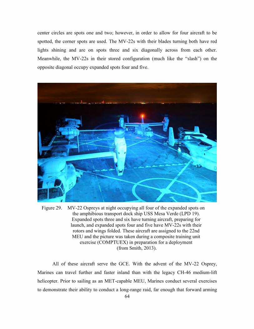
64

center circles are spots one and two; however, in order to allow for four aircraft to be

spotted, the corner spots are used. The MV-22s with their blades turning both have red

lights shining and are on spots three and six diagonally across from each other.

Meanwhile, the MV-22s in their stored configuration (much like the “slash”) on the

opposite diagonal occupy expanded spots four and five.

Figure 29. MV-22 Ospreys at night occupying all four of the expanded spots on

the amphibious transport dock ship USS Mesa Verde (LPD 19). Expanded spots three and six have turning aircraft, preparing for launch, and expanded spots four and five have MV-22s with their rotors and wings folded. These aircraft are assigned to the 22nd MEU and the picture was taken during a composite training unit

exercise (COMPTUEX) in preparation for a deployment (from Smith, 2013).

All of these aircraft serve the GCE. With the advent of the MV-22 Osprey,

Marines can travel further and faster inland than with the legacy CH-46 medium-lift

helicopter. Prior to sailing as an MET-capable MEU, Marines conduct several exercises

to demonstrate their ability to conduct a long-range raid, far enough that forward arming

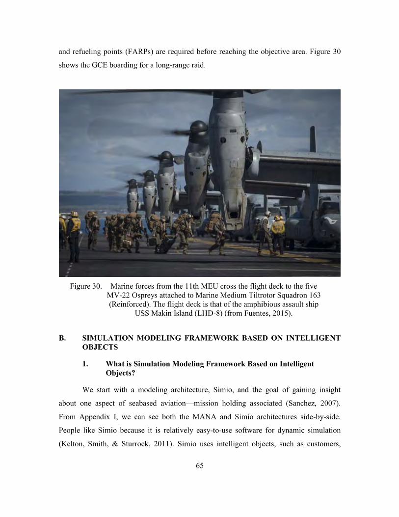
65

and refueling points (FARPs) are required before reaching the objective area. Figure 30

shows the GCE boarding for a long-range raid.

Figure 30. Marine forces from the 11th MEU cross the flight deck to the five

MV-22 Ospreys attached to Marine Medium Tiltrotor Squadron 163 (Reinforced). The flight deck is that of the amphibious assault ship

USS Makin Island (LHD-8) (from Fuentes, 2015).

B. SIMULATION MODELING FRAMEWORK BASED ON INTELLIGENT OBJECTS

1. What is Simulation Modeling Framework Based on Intelligent Objects?

We start with a modeling architecture, Simio, and the goal of gaining insight

about one aspect of seabased aviation—mission holding associated (Sanchez, 2007).

From Appendix I, we can see both the MANA and Simio architectures side-by-side.

People like Simio because it is relatively easy-to-use software for dynamic simulation

(Kelton, Smith, & Sturrock, 2011). Simio uses intelligent objects, such as customers,

66

infantry, or aircraft, in conjunction with the physical components of the system they are

in to model and reflect dynamic interactions of entities within a system. Simio works well

for DES, specifically discrete event, stochastic, models for solving problems (Kelton et

al., 2011). Simio was industrialized by the same people that developed Arena (another

type of DES that has been widely used), but leverages early instances of object-oriented

modeling, which grew into the Simio of today (Kelton et al., 2011).

2. Benefits of Simio

Simio is intuitive and easy to use. Once all the objects are created, they can be

used in multiple simulation models. For the Marine Corps, this is highly useful because

of the combined visuals, ease of use, and building-block nature to advanced modeling.

Below is a list that summarizes the benefits of Simio.

Visualization—a Simio model looks like the real system.

As with many software programs, with Simio it is easy to build large models of increased complexity from initial toy models.

Simio objects can be used for multiple models.

Simio objects can readily be reused and combined to build process models.

Process models can be easily adjusted and experimented with to gain insights.

Many experiments can be run (i.e., thousands of replications) and results are collected in pivot tables that may be exported to an XML file for analysis. (Simio LLC, 2010)

3. Simio: Limitations and Assumptions

a. Limitations of Simio

Simio is limited by the level of detail provided to each object by the user and the

Simio environment. In this first-stage, launch constraint, model the focus was a long-

range raid and any holding that transpired during the entire operation. The aircraft agents

in Simio all takeoff and “launch” with the same flight characteristics and profile.

However, this is known not to be the case for MV-22, CH-53K, F-35B, etc. Therefore, a

67

limitation in Simio is that the modeled system might not reflect the complexity of the real

system. In aviation, winds, pitch, and roll of the ship, and temperature can alter fuel

consumption rates. During flight operations, naval traffic can preclude aircraft from

landing until the ship alters course. Yet, all of these, to include the unique takeoff profile

of dissimilar aircraft did little to inform the MOEs. Different launches and flight

conditions, which could have been modeled were not, however, this model had the right

level of precision to make it valid for the purposes of this broad analysis (Kelton, 2011).

b. Assumptions Made in Simio

The primary assumptions in this Simio model are that times for mission holding

and launch are distributed with a triangular distribution. The simulation is used to better

understand launch constraints and aircraft flight operations.

Triangular distributions are assigned for service times (e.g., LPD slash, fuel/arm).

Aircraft objects – the launch process is roughly similar for all types of aircraft and they are modeled by the same process.

A launch includes removing an aircraft from the slash to it being cleared for takeoff.

The flight schedule launch times representative of a flight schedule are generated from a time varying arrival process with hourly granularity.

Aircraft from the LHD require mission holding to constitute the package.

The LPD has one slash, two spots, one fuel, Arm/De-arm, and one chains crew.

The LHD has two slashes, three spots, one fuel, Arm/De-arm, and one chains crew.

C. RESEARCH QUESTIONS

This first stage model is valuable as it generates realistic inputs to the MANA

second stage model. Additionally, one may adjust the first stage model independent of

the larger amphibious model, which may be useful for energy-specific insights related to

air operations. While this Simio model focuses on the flight-deck cycle, one could easy

apply a first stage model like this to explore other key areas in amphibious assault. One

68

such application is instead of using aircraft launching from the flight deck, use ACV

departing the LCAC, or infantry departing the ACV.

The questions guiding this first stage model are:

Are there OE2 benefits to conducting distributed ops?

Are there OE2 benefits to conducting split ops?

Addressed in this section are EW 12 aviation-seabase-related particulars that are

applicable to the deck cycle, and how those were implemented in Simio. We also provide

further details about the objects in Simio and an overview of the system.

D. MEASURES OF EFFECTIVENESS

The purpose of this simulation is to provide a specific look into the OE2 of the

ACE launching from the seabase in support of amphibious operations. Here, our MOEs

include:

MOE (5): Mission Holding

MOE (6): Mission Total Time

E. SCENARIOS

Modeled is a 14-aircraft package launched in support of a long-range raid, which

requires a FARP. There are three available spots on the LHD and two expanded spots on

the LPD. The SAR aircraft is required throughout flight operations, and the SAR SH-60

must have a free spot to land on at all times.

Covered here are:

The three scenarios modeled in Simio: All-LHD, Split, and Disaggregated Operations (Ops).

Modeling particulars.

Details on the Time Varying Arrival Rate Table (“flight schedule”), servers, and objects.

69

F. MODELING PARTICULARS

1. Source

The source node for this long-range raid creates a maximum of 14 total aircraft to

be launched from the ARG. The source is used to initiate launches according to a time-

varying rate table and these launches may be probabilistically assigned to ships according

to the scenario modeled. Aircraft may launch from either of the two ships: the LHD and

the LPD. Aircraft may also be pulled from either the forward or the aft slash on the LHD

to support the required package. The Marine ACE holds when launched from the LHD.

The ACE aircraft are:

A single SAR SH-60.

A section of AH-1Z Super Cobras (attack and escort).

A section of F-35B (attack and escort).

A command and control UH-1Y (air mission commander platform).

Six MV-22 Ospreys providing the required lift for the minimum required force and go criteria for the GCE.

A section of CH-53Ks for the FARPs.

Table 5 lays out how many deck spots, slash areas, and crews are modeled in the

three options described to compare the resources available. Split and disaggregated ops in

the context of Table 5, are split ops 12/14 aircraft on the LHA and disaggregated ops

10/14 aircraft on the LHA.

Table 5. The three options modeled are: all aircraft launching from the LHD, the split, and disaggregated operations. Aircraft launched from the LHD have two slashes (forward and aft), three spots, and one crew to facilitate the launch sequence. No LPD slash, spots, or crew are available in “all from

LHD” operations.

Slash Spots Crews Operations Prop_LHA LHD LPD LHD LPD LHD LPD All from LHD 1.0 2 0 3 0 1 0 Split 12/14 = 0.857 2 1 3 2 1 1 Disaggregated 10/14 = 0.714 2 1 3 2 1 1

70

The mission modeled is a long-range raid. The composition is 14 aircraft

launched in any of the three operations listed in Table 5. The model focuses on the

origination options, which may either be all from the LHD, the split, or disaggregated.

A requirement (to satisfy it being a long-range raid) is a FARP. From the

origination options described, aircraft hold as required to constitute the package, transit to

the objective area, and then FARP. The FARP mission is the responsibility of a section of

CH-53Ks. The FARP has four fuel points, capable of providing gas to running aircraft in

four fixed spots (a “hot static FARP”). The CH-53Ks are likely FARP platforms since

they provide internal fuel stores that support bulk refueling.

The single-ship SH-60 facilitates the SAR mission, serving as the SAR aircraft.

This aircraft is required for rotary and tilt-rotor operations. Of note, spot two on the LHD

is dedicated for SAR operations and cannot be spotted with ACE aircraft.

Two AH-1Zs, one UH-1Y, and two F-35Bs provide escort, command and control,

strike, and close air support. These aircraft all safeguard the GCE flying aboard six

MV-22s. Thus, with the originations described, 2 AHs, 1 UH, 6 MVs, 2 F-35s, 1 SH, and

2 CHs, totaling 14 aircraft, are modeled.

Link weights are used to facilitate spilt and disaggregated operations. A link

weight of zero bars split operations, forcing all 14 aircraft to launch from LHD. For this,

a numeric property was assigned to the path connecting the source node to either the LPD

slash or the transfer node, leading to the LHD forward and aft slashes.

2. Time-Varying Arrival Rate Table

The flight schedule was created to support the package described. The real-world

process modeled is the initiation of the launch process for individual aircraft. This is

modeled from a time-varying arrival rate pulled from a rate table. Table 6 shows the

Time-Varying Arrival Rate Table.

71

Table 6. This Time Varying Arrival Rate Table shows the launch of a section of AHs within the first 30 minutes of flight operations, followed by the GCE aboard

six MV-22s in the next 30 minutes, followed by the SAR, FARP, and command and control aircraft, until, lastly, the F-35Bs are launched.

Starting Offset Ending Offset Rate (events per hour) Day1, 00:00:00 Day 1, 00:30:00 2 AHs Day1, 00:30:00 Day 1, 01:00:00 6 MVs Day1, 01:00:00 Day 1, 01:30:00 1 UHs, 1 SHs, 2 CHs Day1, 01:30:00 Day 1, 02:00:00 2 F-35Bs

Another reason for the rate table is that the F-35B requires a deck run, and the

sequencing of aircraft from and to the spots is dictated this way in practice.

3. Seabase

Scenarios include split and disaggregated operations (with the LPD), and all from

LHD operations (without the LPD).

a. Launch Process: LHD

(1) Forward Slash

Subsequent to the initiation of a launch, the time required to position the aircraft

is a random variable draw from a random triangular distribution that “draws” with a

minimum of 15 minutes, mode of 30 minutes, and maximum of 50 minutes. We represent

this distribution the following way: T~Tri(x,y,z), where the forward slash is S~Tri(15, 30,

50). Thirty minutes is a commonly accepted length of time to tow an aircraft out of the

slash and bring it to its spot.

(2) Aft Slash

Follows the same parameters as the forward slash: S~Tri(15, 30, 50).

(3) Resource Node

Following aircraft being spotted to the initiation of takeoff, the time required for

fueling, breaking down the chocks and chains, arming, and the launching of an aircraft

once they are spotted is a random variable draw from a random triangular distribution

that “draws” with L~Tri(3, 5, 10) for the LHD. This modeled Simio is a limited resource

72

that has one fixed capacity and First In, First Out logic. This embodies the limitations of

ordnance and fueling crews available to service one spot on the flight deck at a time.

(4) Mission Holding

Following takeoff, the holding time required for creating the flight package is a

random variable draw from a random triangular distribution that “draws” H~Tri(5, 10,

20). Disparate aircraft traveling on different routes after takeoff from the LHD hold

linkup for the subsequent transit, objective area, and FARP portions of the mission.

b. LPD

(1) Slash

Follows the same parameters as the forward and aft slash of the LHD; however,

they are distributed as SL~Tri(2, 5, 7). Aircraft slashed on the expanded spots are more

readily available for prelaunch procedures than those aboard the LHD once flight quarters

are sounded. Flight quarters occurs when a ship may is postured to safely conduct flight

operations. Removing them from the LPD slash often does not entail any aircraft

movement at all (see Figure 30).

(2) Resource Node:

Spotted aircraft on the LPD perform the launch sequence, which is a random

variable draw from a random triangular distribution that “draws” with LL~Tri(2, 3, 5) for

the LPD.

c. Transit to the Objective Area, Objective Area Time on Station, FARP

Time and Sink

After the package is constituted, aircraft depart the rendezvous point and transit to

the objective area and FARP location with transit time, TT, where TT~Tri(40, 60, 120).

The subsequent objective area time on station, TOS, where TOS~Tri(20, 30, 45) and

FARP time, FT, where FT~Tri(15, 20, 45) support disparate aircraft, traveling on

different routes, of varying times, over a broad range of likely missions. All three (transit

time to the objective area, objective area time on station, and FARP time) follow random

triangular distributions.

73

Upon completion in the FARP, aircraft depart the process. In Simio, objects check

out of the system via a sink node. At 10 hours, the simulation ends, with the package of

aircraft all having arrived at the sink.

Figure 31 shows a screen shot of the final simulation effort done in Simio.

Figure 31. Screen shot of the Simio simulation.

In summary, this section reviewed Simio and its usefulness for discrete event

simulations, particularly aircraft launch constraints. We saw a varying arrival rate table

operationally simulates the flight schedule. Finally, we learned about how agents, arrival

times, resource nodes, and servers were used to model a long-rang raid evolution that

included a FARP.

74


75

VI. DATA ANALYSIS AND RESULTS

Gatchel sums up a sea power’s advantage this way: In spite of the availability of modern ground and air transportation to defenders today, navies continue to maintain their traditional mobility advantage…no army can move with enough combat power to repulse a major assault before the landing force has established itself ashore.

—CAPT Wayne P. Hughes, Jr., USN (Ret)

In this chapter, we analyze the data generated from the experiments described in

the previous chapters, and present main insights.

A. JMP DATA ANALYSIS TOOL

JMP is statistical analysis software that provides the capability for analysts to

visualize and analyze data, including metamodel fitting. JMP can also be used for data

manipulation prior to analysis. For example, data was concatenated, sorted, and organized

in JMP. The tools in JMP can create interactive linked graphs, display data histograms and

statistical summaries, as well as perform regression analysis and other multivariate

methods. JMP also has a useful journal feature that allows the user to save and organize

artifacts of the analysis. One of the most attractive features of JMP is its intuitive, context-

dependent, menu-driven interface (Suite of Analytics Software [SAS], 2014).

B. ANALYSIS OF AMPHIBIOUS ASSAULT EXPERIMENT

First we present the four MOEs used in this analysis.

MOE (1): Blue casualties

MOE (2): Red casualties

MOE (3): Time to attrite the Red Force to one-third remaining strength

MOE (4): FER, which is calculated as (Red casualties +1)/(Blue casualties +1)

Let us now review our scenarios as they relate to the results:

1. LCAC (ACV) only

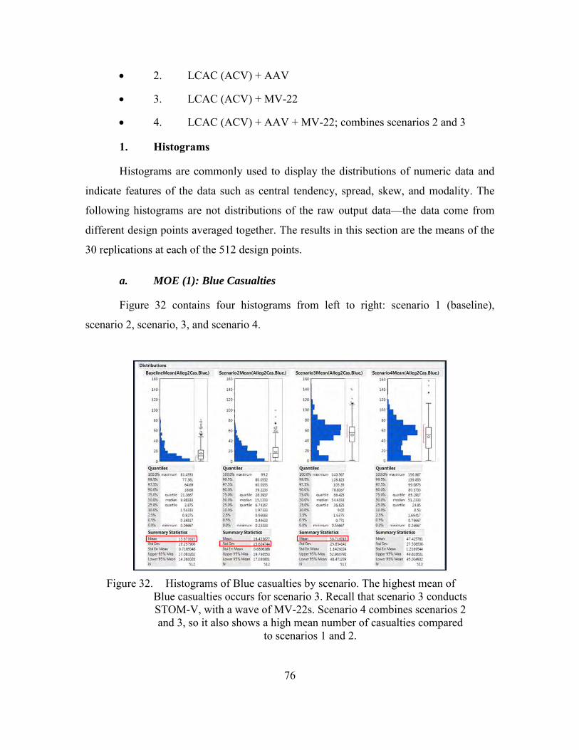
76

2. LCAC (ACV) + AAV

3. LCAC (ACV) + MV-22

4. LCAC (ACV) + AAV + MV-22; combines scenarios 2 and 3

1. Histograms

Histograms are commonly used to display the distributions of numeric data and

indicate features of the data such as central tendency, spread, skew, and modality. The

following histograms are not distributions of the raw output data—the data come from

different design points averaged together. The results in this section are the means of the

30 replications at each of the 512 design points.

a. MOE (1): Blue Casualties

Figure 32 contains four histograms from left to right: scenario 1 (baseline),

scenario 2, scenario, 3, and scenario 4.

Figure 32. Histograms of Blue casualties by scenario. The highest mean of

Blue casualties occurs for scenario 3. Recall that scenario 3 conducts STOM-V, with a wave of MV-22s. Scenario 4 combines scenarios 2 and 3, so it also shows a high mean number of casualties compared

to scenarios 1 and 2.

77

To the right of each histogram is a box plot. Box plots will be covered in Section

2. Below the histograms are quantiles and summary statistics, including the means.

Scenario 3 has the highest average Blue casualties and scenario 1 has the fewest. We note

that standard deviation is the smallest during scenario 2. The first two scenario

histograms are positively skewed. Scenarios three and four are bimodal, with peaks near

50 casualties and 10 casualties.

Blue casualties are greatest in scenario 3, when Blue is brought in via MV-22s,

which means that infantry are more vulnerable than when they are entirely inside ACVs.

Scenario 4, which combines scenarios 2 and 3, is associated with greater numbers of

casualties than either the ACV or ACV and AAV scenarios.

b. MOE (2): Red Casualties

Figure 33 contains histograms, box plots, and summary statistics for Red

casualties.

Figure 33. Red casualties are greatest when Blue attacks with ACVs and AAVs

in both scenarios 2 and 4. Red’s survival is better when Blue does not use the AAVs. Red casualties experience little change from scenario 1 to 3. Scenarios 2 and 4, each have waves of AAVs

accompanying ACVs onboard LCACs.

78

The highest mean Red casualties occur with scenario 4; however, scenario 2 has a

slightly higher median number of casualties. In any case, scenarios 2 and 4 are very

similar. Scenarios 1 and 3 are also similar with respect to this MOE. Red casualties are

greatest when Blue attacks with AAVs and ACVs in both scenarios 2 and 4. In scenario

4, Blue attacks with a combined force from AAVs/ACVs and infantry brought in from

MV-22s. This scenario’s strength does not appear to be the MV-22, based on the

insignificant increase from scenarios 1 to 3, but rather the AAV. All four scenarios,

interestingly enough, are negatively skewed, as evidenced by the long tails toward low

casualties (circled in the figure) Nevertheless, Red casualties are lower, with a higher

frequency when the AAV is not present, as in scenario 3.

c. MOE (3): Time to Attrite the Red Force to One-Third Remaining

Strength

Figure 34 contains the histograms, box plots, and summary statistics for time to attrite the

Red force to one-third remaining strength, where the fastest mean time occurs with scenario 4.

Figure 34. Time to attrite the Red force to one-third remaining strength, where

the fastest mean time occurs with scenario 4. This objective is not met 84 times with scenario 1 (512 – 428 = 84). Meanwhile, scenario 2 has the lowest standard deviation and higher times can be expected

with scenario 3, seen in the circled portion of the data.

79

There is, however, overlap, as seen with scenarios 1 and 3. The greater frequency

of long times for scenario 3 makes sense, given the scenario 3 Blue casualty numbers. It

is important to realize, in general, that achieving one-third remaining strength might not

always happen. This explains why N is less than 512 for each of the scenarios. We

achieve this MOE the fewest times during scenario 1—namely, that Blue is slower to

mass and attrite Red.

There is good cause for us to revisit the raw output data, since if one design point

attrites the enemy in only half of the replications—but when it does, does so quickly—a

low Mean (RedKillTime) only tells part of the story. Therefore, a wise approach is to

create a column next to the FER in the full data that is a binary result, where success is

attriting Red to one-third of its remaining forces. Figure 35 shows the probability of

attriting Red to the desired level.

.

80

Figure 35. Realized probability for attriting Red to one-third of its remaining

forces.

Distributions Scenuio= 1

AttrltetoOneThkd

.I 0 I

Distributions Scenuio=2

AttrltetoOneThkd

I. 0 I

Distributions Scenuioa 3

AttrltetoOneThkd

0 I

Distributions Scenuio=4

AttrltetoOneThkd

I. 0 I

Frequendes

l evel Count Prob )410 0.22'201

119SO~ 1Sl60~

0 I , ....

0

Frcquenc:kt

l evel Count Prob 1116~ 14244~ 1Sl60 1..oooo:l

0 I

0

Frequendes

l evel Count Prob 0 1 , ....

ll$;1~ llUi~ 1Sl60 1..oooo:l

0

Frequendes

l evel Count Prob 1070~ 14290~ 1Sl60 1..oooo:l

0 I

0

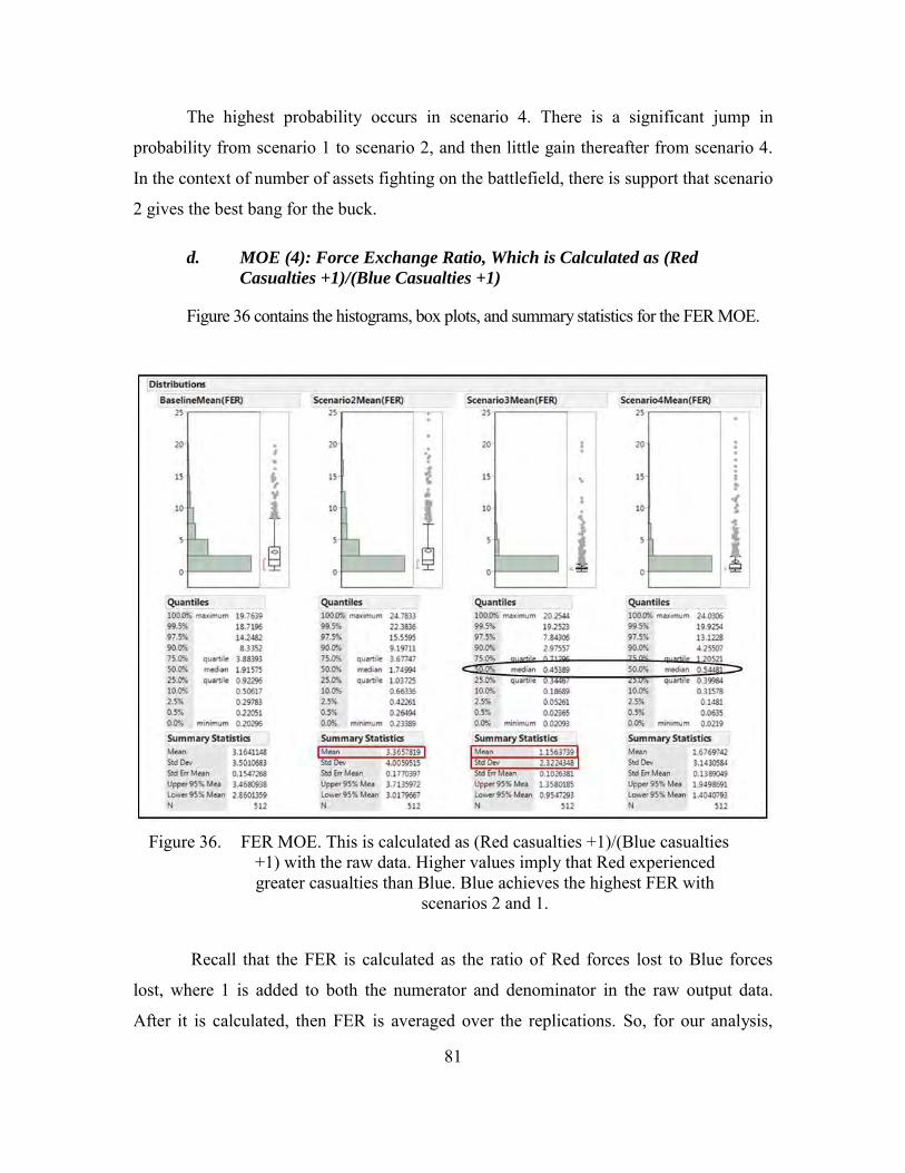
81

The highest probability occurs in scenario 4. There is a significant jump in

probability from scenario 1 to scenario 2, and then little gain thereafter from scenario 4.

In the context of number of assets fighting on the battlefield, there is support that scenario

2 gives the best bang for the buck.

d. MOE (4): Force Exchange Ratio, Which is Calculated as (Red

Casualties +1)/(Blue Casualties +1)

Figure 36 contains the histograms, box plots, and summary statistics for the FER MOE.

Figure 36. FER MOE. This is calculated as (Red casualties +1)/(Blue casualties

+1) with the raw data. Higher values imply that Red experienced greater casualties than Blue. Blue achieves the highest FER with

scenarios 2 and 1.

Recall that the FER is calculated as the ratio of Red forces lost to Blue forces

lost, where 1 is added to both the numerator and denominator in the raw output data.

After it is calculated, then FER is averaged over the replications. So, for our analysis,

82

higher is better. If the FER is high, as it is in scenario 2, that means that Blue is losing far

fewer casualties than Red. The FERs for scenarios 1 and 2 are similar, and the FERs for

scenarios 3 and 4 are similar. Nevertheless, when Blue is inside vehicles, Red loses

casualties at a larger rate than Blue, as evidenced by the higher FERs in scenarios 1 and

2. The impact from bringing forces in via helicopter exposes infantry earlier in the

amphibious assault and makes them more vulnerable, resulting in more Blue casualties

and fewer Red casualties.

FER is another example where the raw output data may provide insights that

could perhaps be lost during means analysis. Figure 37 shows the scenarios with the

highest mean FER (scenario 2) and lowest mean FER (scenario 3).

Figure 37. FER MOE with raw output data. Highest is scenario 2 and the

lowest is scenario 3.

83

One final comparison can be made between the FER and Blue casualties.

Analytically, we observe that since Blue casualties are in the denominator of the rational

fraction, that a higher FER signals a greater loss ratio of Red to Blue. Figure 38 shows Blue

casualties on the y-axis, with the scenario across the bottom, and FER across the top.

Figure 38. Relationship between Blue casualties (y-axis) and FER (top), by

scenario. Higher Blue casualties are seen at the far left when FER is the lowest.

2. Box Plots

Next, we look at the output with box plots. Although they were part of the output

in the previous section, we will cover them more in depth in this section. It can be useful,

for example, to display box plots grouped by levels of a categorical variable. Figure 39

shows an illustration of box plot.

84

Figure 39. Depicted is a box plot. Box plots in JMP have whiskers that extend

out to 1.5 times the interquartile range (IQR). The boxed region shaded in gray represents the IQR, bounded by the 25th and 75th

quantiles. JMP depicts outliers with large dots that fall outside of 1.5 times the IQR (from Lucas, 2014).

a. MOE (1) and MOE (2)

Figure 40 shows a side-by-side comparison of Blue and Red casualties.

Figure 40. This figure shows that there is little difference for Red between

scenarios 2 and 4, while Blue incurs many more casualties in scenarios 3 and 4.

85

Note that the vertical axes on the two plots are different. These plots confirm that

scenarios 3 and 4 have higher Blue casualties, but that scenario 4 has an IQR that covers

more of the lower-casualty range. Similarly, Red incurs fewer casualties in scenarios 1

and 3, and more casualties in scenarios 2 and 4.

Figure 41 contains box plots for Blue casualties’ MOE and Red casualties, this

time grouped by scenario, number of LCACs (right vertical axis), and debark distance

(across the top).

Figure 41. The Blue casualties’ plot on the left shows that Blue casualties are

more influenced by scenario than by debark distance or number of LCACs. The Red casualties’ plot on the right shows that Red

casualties are influenced by debark distance, LCAC count, and scenario.

The plot on the left shows Blue’s casualties from scenarios 3 and 4 are higher for

all nine possible configurations. Further, Blue casualties do not seem to be affected by the

number of LCACs. Meanwhile, the plot of Red casualties on the right shows that they are

the highest when Blue debarks from less than five nm and greater than three LCACs

(outside the circle). Casualties for Red are less with higher frequency inside the circle.

In order to get a better understanding of Blue casualties, we plot the mean number

of Blue infantry squad casualties by scenario and squad number to gain insight into which

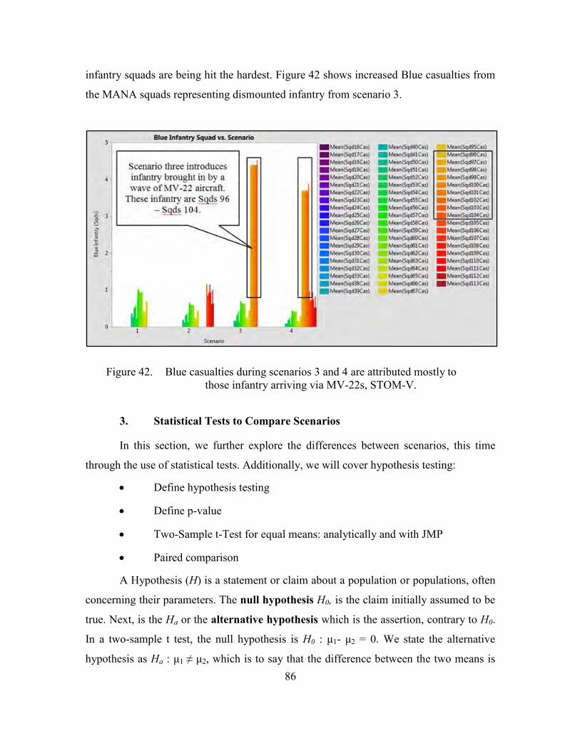
86

infantry squads are being hit the hardest. Figure 42 shows increased Blue casualties from

the MANA squads representing dismounted infantry from scenario 3.

Figure 42. Blue casualties during scenarios 3 and 4 are attributed mostly to those infantry arriving via MV-22s, STOM-V.

3. Statistical Tests to Compare Scenarios

In this section, we further explore the differences between scenarios, this time

through the use of statistical tests. Additionally, we will cover hypothesis testing:

Define hypothesis testing

Define p-value

Two-Sample t-Test for equal means: analytically and with JMP

Paired comparison

A Hypothesis (H) is a statement or claim about a population or populations, often

concerning their parameters. The null hypothesis H0, is the claim initially assumed to be

true. Next, is the Ha or the alternative hypothesis which is the assertion, contrary to H0. In a two-sample t test, the null hypothesis is H0 : μ1- μ2 = 0. We state the alternative

hypothesis as Ha : μ1 ≠ μ2, which is to say that the difference between the two means is

87

not equal to zero. In other words, we claim that the means are the same and research

whether this is the case. Often the Ha is called the research hypothesis; however, the

burden of proof required is to disprove H0. Proof is measured by evaluating the p-value.

P-value is the probability of seeing data this extreme or more extreme, assuming that the

H0 is true. The proof in this section will be shown graphically, calculating it analytically

requires the appropriate test statistic value. The two-sample t test for the means test

statistic analytical formula (see, e.g., Wackerly, Mendenhall, & Scheaffer, 2008) follows:

𝑡 =�̅� − �̅�

√𝑠12

𝑛1+𝑠22

𝑛2

Paired testing compares the outcomes between two scenarios under the same

conditions. This is why it is often called paired comparison, which is a one-sample test

on the differences of the data. For example, a paired comparison between scenario 2 and

scenario 4, with the response “Red casualties” MOE, would subtract the Red casualty

outputs from scenarios 2 and 4, respectively, at each of the 512 design points. The

histograms showed high variability across many of the MOEs by scenario. If we detect

higher variability from averaging, then the associated two-sample problem may not

reflect the detail we seek, which is why a paired comparison between scenarios 2 and 4,

without incorporating the differences from it being scenarios 2 and 4, is preferred. The

analogy for paired comparisons with multiple samples is to treat each design point as a

block when performing ANOVA.

a. Scenario: Two-Sample t Test; One-Way Analysis of Variance of Red

Casualties by Scenario

Figure 43 contains an excerpt of the result of the Analysis of Variance (ANOVA)

procedure of mean Red casualties by scenario. The y-axis is the mean number of Red

casualties, the x-axis represents the scenario, and a horizontal line at 23 represents the

overall mean of the response. We report the results without blocking on design point, and

note that blocking reduces p-values (showing higher levels of statistical significance) but

does not change the qualitative conclusions. Appendix C contains the full results of the

ANOVA procedure of mean Red casualties by scenario. In addition, Appendix D

contains the study for the raw output data.

88

Figure 43. This plot shows a one-way analysis of the summarized output

(2,048 rows) for “Red casualties” by scenario, with the number of Red casualties on the vertical axis. In red, we see overlapping circles

for scenarios 1 and 3. Scenarios 2 and 4 have similar boxplots and circles which are “overlapped.”

Figure 44 shows a Connecting Letters Report and the confidence level used.

Scenarios 4 and 2 are designated with “A” and scenarios 3 and 1 are designated with “B.”

Figure 44. Connecting Letters Report at the 95% confidence level.

89

Another way to summarize the comparison of the mean number of Red casualties

across scenarios is with an Ordered Differences Report. In this report, the difference

between each pair of scenarios is summarized with a mean difference, as well as a

confidence interval and p-value. What is valuable about this report is that it shows ranked

differences between scenarios, with scenarios 4 and 1 being the most different and 4 and

2 being the least. Figure 45 shows the ordered differences report, and the red box shows

the dissimilar scenario groupings.

Figure 45. The Ordered Differences Report.

We now repeat the ANOVA using the full set of output (using data from all

design points and replications), vice just the 2,048 points, where each design point was

summarized by its mean. Figure 46 shows the result of the ANOVA test on the full

output. This result is similar to the previous result, except that this time, scenarios 3 and 1

(connecting letters B and C) are deemed significantly different.

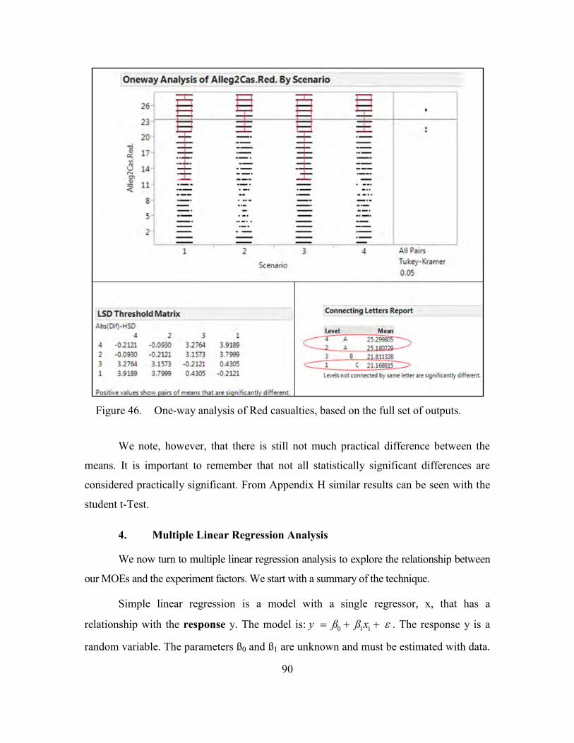
90

Figure 46. One-way analysis of Red casualties, based on the full set of outputs.

We note, however, that there is still not much practical difference between the

means. It is important to remember that not all statistically significant differences are

considered practically significant. From Appendix H similar results can be seen with the

student t-Test.

4. Multiple Linear Regression Analysis

We now turn to multiple linear regression analysis to explore the relationship between

our MOEs and the experiment factors. We start with a summary of the technique.

Simple linear regression is a model with a single regressor, x, that has a

relationship with the response y. The model is: 0 1 1 y ß ß x . The response y is a

random variable. The parameters ß0 and ß1 are unknown and must be estimated with data.

91

To transition to multiple regression variables or regressors you add more terms. Here we

will also consider interaction terms ( 1 2x x ) and polynomial terms to degree two

( 21x ). Equation 2 shows the full second-order fitted multiple linear regression model for

two regressors, 1x and 2x .

2 20 1 1 2 2 3 1 2 4 1 5 2y x x x x x x (2)

How well the model fits the data is measured with R Squared, root mean squared

error, and plots of the errors from our actual versus predicted values. R Squared

indicates what percentage of the variability is explained by the regression model. If our

interest were prediction, additional model adequacy checks could involve assessing the

whether the errors are distributed normally with constant variance 2 . Fortunately, the

estimated regression coefficients are robust to departures from normality and constant

variance, so the regression models can be used to identify the most important factors and

identify the nature of the relationship between these factors and the response.

a. Main Effects

The first fitted model is the main effects model for Blue casualties. This model

was fit using the stepwise functionality in JMP. Both “mixed” and “forward” were used

in model generation. Between BIC and p-value with p < 0.01 to enter and exit the model,

p-value seemed to give the better models. The selected mode using Standard Least

Squares and effect screening has an R squared of 0.53. The model has 17 terms, with the

most important factor being scenario 3. Figure 47 shows the summary of fit for the full

output and the most important parameters in the sorted parameter estimates s .

Figure 47. Full uncompressed output, “Blue casualties.” Scenario 3 increases

“Blue casualties,” while scenarios 2 and 1 decrease “Blue casualties.”

92

Figure 47 shows that “Blue casualties” are heavily influenced by scenario 3. As a

matter of fact “Blue casualties” are higher in scenario 3 than in scenarios 1 and 2.

Increases in InfHit2k (i.e., infantry hit to kill) decreases “Blue casualties.” Not listed is

anything pertaining to speed.

Figure 48 shows that “Red casualties” increase with ACV speed, LCAC count,

LCAC speed, and scenario 2. “Red casualties” decrease with ACV debark distance,

scenario 1, and scenario 3. Not listed in is anything pertaining to force protection or hits

to kill.

Figure 48. Full uncompressed output, “Red casualties” depend on ACV speed,

debark distance, LCAC quantity, and LCAC speed.

Figure 49 shows the prediction profiler for “Red casualties.” The figure on the left

supports fast LCACs, AAVs, and ACVs. The plots on the right support larger numbers of

“Red casualties” with scenarios 2 and 4; however, they make a case for debark distances

of 5 nm and 12 nm, and three or more LCACs.

Figure 49. Red casualties increase with all three speeds: LCAC, AAV, and

ACV. Similarly, scenarios 2 and 4, and LCAC quantities of three and four increase the number of Red casualties. “Red casualties”

decrease when the ACVs are debarked further than 12 nm from the shore.

93

The most important factors for “Red casualties” continue to be speed, quantity,

and scenario dependent, which perhaps is justification for pursuing further “Red

casualty” MOEs.

Finally, we look at the “time” MOE. In a main effects only model, with 12 terms,

the “time to attrite Red to one-third remaining strength” is affected, as one would expect,

by speed and distance. The speed that contributes most to the MOE is the ACV speed, not

the LCAC speed. LCAC speed and LCAC quantity all decrease the “time” MOE.

Meanwhile, debark distance and scenario 1 increase it. Figure 50 shows the “time” MOE

summary of fit. A partition tree (not shown) of the probability of attriting red to one-third

of its original forces gives similar results: ACV speed and debark distance are the two

most influential factors.

Figure 50. “Time” MOE. ACV speed contributes most to reducing the “time to

attrite Red Force to one-third remaining strength.” Debark distances and scenario 1 take longer to attrite Red to the desired level.

With regard to the number of LCACs and the debark distance, Figure 50 shows

the following added benefit and importance:

Being at 5 nm is extremely important.

Scenarios 2 and 4 are preferred.

Going from 2 to 3 LCACs helps much more than going from 3 to 4 LCACs.

Thus, for the “time” MOE, it increases with distance; however, the benefit of

going from two to three LCACs is much greater than from three to four. Figure 51 shows

the prediction profiler for scenario, debark distance, and LCAC quantity.

94

Figure 51. The “time” MOE and how scenario, ACV debark distance, and

LCAC quantity compare.

b. Comparison of Main Effects

In this section we fit simple main effect models for the MOEs. These models

reflect the primary variables, and support general insights. The summary of fit and the

sorted parameter estimates are provided below. Figure 52 shows Blue casualties” on the

left and “Red casualties on the right.

Figure 52. The main effect models for Blue and Red casualties.

At the top of the figure are the R Squared values that measure how much of the

variance is explained by the model below. This measure of observed variance is often

referred to as goodness of fit. Meanwhile, the sorted plots below show the model in a

ranked column that depicts most influence to least. Each term has an estimate, standard

error, t-ratio, shaded horizontal bar, and Prob >|t|. First, the estimate signals that the

95

“Blue casualties,” for example, will increase by 17.6 casualties if in scenario three. The

most significant factor for Blue is scenario, while for “Red casualties” it is ACV speed.

Significance is seen from both the t-ratio and Prob >|t|. In another example, seen with

“Red casualties” there are nine terms that have t-ratios greater than four, likewise “Blue

casualties” only has four. Also, for Blue those four are really just levels of scenario and

LCAC speed. Figure 53 shows the main effects models for FER and “time” MOE.

Figure 53. The main effect models for FER and “time” MOE.

(1) Discussion

From the summary of fits, we see that the highest R Square is attained with the

time it takes to attrite red to one-third strength. Other R Squares are 0.38 or less with the

lowest being FER. Depending on the MOE selected above at most 50% of the variability

could be explained by these main effects, while the worst is 10%. Combat is inherently

difficult to predict, which means that these values are actually doing well, but should be

used for comparison rather than prediction.

For Blue casualties, there are benefits to ACV debarking at closer distances (e.g.,

“LCDbkDist [25-12]”), namely that Blue benefits from being inside 12 nm. However,

this benefit is nothing compared to that of being in scenarios one and two. One might

make many more replications to support the impact from “LCACMvtSpd” or LCAC

speed.

96

Indeed, “Red casualties “increase with and decrease with varying signs through

nine different parameters. ACV speed, LCAC quantity, speed, and scenario two are

increase Red casualties. Scenarios one and three decrease casualties.

(2) Most Important Factors

Blue: The most important factors are scenario and distance. It is not clear that Blue experiences a benefit from speed. As a matter of fact we see that LCAC speed and scenario three with fast aircraft, increase Blues losses. Blue vehicles are arriving to the objective and dismounting infantry. A byproduct of the design that was not anticipated was that with scenario two there are more vehicles which increase both the weapons and armored personnel carriers to distribute the force across.

Red: Speed and quantity increase red casualties most. Incidentally ACV and LCAC should be made fast before the AAV. Debark distances beyond 12 nm and scenario 1 decrease casualties more than scenario 3.

FER/time: With differing information for MOE one and two, we turn to FER and the “time” MOE. The two most important factors seen from FER and “time” to give Blue an advantage are scenario and speed. Blue might seek to get into scenario 2 most often and initially explore investments in speed in the ACV.

(3) Insights

Two general insights are discovered from the evidence presented from the main

effect models.

FLOT speed: The basic concept is that speed works to a certain point. Blue infantry arriving in MV-22 outpace the time required to mass force ashore. In the “time” MOE we get a sense for the right pace. ACV speed, LCAC speed, and multiple connectors create a good pace.

Force protection: What is not seen is a mention of infantry hits to kill, concealment, or number of agents. Red consists of a formidable force of 28 agents. To give the defending force the advantage 18 Red infantry require 11 hits to kill, and are 70% concealed. The force in the defense has increased staying power and defensibility. Force protection is nested in the increased casualties from scenario 3; however, it is not explicitly influential to the attacking force.

A battle is challenging to predict. R squared captures that stochastic behavior of

agents interacting and responding to what their sensors are telling them. This research

does incorporate 77 of the prominent tangibles associated with amphibious assault;

97

however, it does not capture intangibles such as breakdowns, Marine leadership, and

luck.

(4) Major Conclusions and Findings

Dismounts and infantry arriving to the objective incur greater casualties. A self-

deploying capability similar to the AAV increases the number of vehicles that Blue

brings to the fight, which in turn increases fire power and distributes the force to absorb

risk from enemy fire. Channelizing terrain, obstacles, and ambush locations can fix the

attacking force for defending artillery. Conversely, urban terrain does limit line of sight

and trajectory for common projectiles. The risks of urban terrain are not covered here.

Marines will use the next AAV and ACV in a way that must be robust. The AAV was to

gets people ashore safely and efficiently. The solution is not one parameter. Amphibious

assault uses a system of systems, where several parameters are determined and then

reassessed. If an LCAC is attrited the seabase might have to maneuver within 12 nm.

Stochastic models provide results that afford simulation that may return different

solutions, but its ability to predict combat and battle is labored at best.

c. Partition Trees

Another analysis method is partition trees. In these models the dependant variable

is still a MOE. JMP splits on the most influential factor based on “distance” between

points in the collapsed output. Incidentally, this distance is the variance—and for the

Marine Corps’ next combat vehicle baseline and desired values are going to drive the

eventual procurement. Key performance parameters are those items that a program like

the ACV will be assessed against to see if it is proving the warfighter with what is

required.

(1) “Blue Casualties” Partition Tree

While Figure 54 does not show all 77 potential candidate factors, what it shows

was the first and most important split was scenario.

98

Figure 54. “Blue casualties” partition tree.

Furthermore, we are doing a better job explaining the variability in just four splits

with an R Squared of 0.53. A key threshold after splitting on scenario 1 and 2 is ACV

sensor range at 2,192 meters. A less effective sensor increases casualties. Likewise, if

Blue must choose scenario 4 or 3, and if Red infantry can classify targets at distances

greater than 4,208 m, then the ACV and the infantry inside require increased force

protections. Figure 55 shows the split history with R Square value on the y-axis and

number of splits on the x-axis.

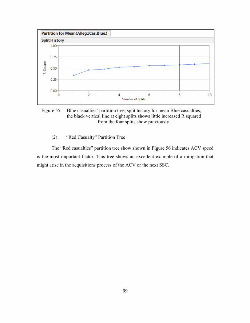
99

Figure 55. Blue casualties’ partition tree, split history for mean Blue casualties,

the black vertical line at eight splits shows little increased R squared from the four splits show previously.

(2) “Red Casualty” Partition Tree

The “Red casualties” partition tree show shown in Figure 56 indicates ACV speed

is the most important factor. This tree shows an excellent example of a mitigation that

might arise in the acquisitions process of the ACV or the next SSC.

100

Figure 56. “Red casualties” partition tree, most import split ACV speed greater

than 16 knots (18 mph).

What if technology readiness level cannot get the ACV to swim and maneuver

on-land at speeds comparable to our top capability, commonly referred to as the speed of

the M1A1? First, the speed of ACV speed splits at 16 knots (18 mph), which is less than

half of the M1A1s speed. Second, the fighting in convention with scenario 2 and 4 in a

slow ACV gives about the same MOE as fighting in a fast one inside 12 nm. The

complexity of amphibious assault and the system of connectors, amphibians, and threat

make the problem tough to break down. This is one approach to refine and quantify what

matters most, when it is all important. Figure 57 shows the split history with R Square

value on the y-axis and number of splits on the x-axis.

101

Figure 57. Red casualties’ partition tree, where more splits might explain more

of the variance.

(3) Main Effects and Partition Tree Comparison of Most Important Factors

The partition trees reflected specific speeds and sensor ranges. The main effects

gave ranked significance levels. Still, the models in the main effects did not satisfy

normal residuals to confirm significance. For the main effects models the most important

factors were not the same. Blue leaned heavily on scenario and Red on speed. For Red

casualties, what was a ranked list of many important factors, now tells a story.

Red casualties: for this MOE there are three important factors, which are ACV speed, scenario, debark distance, ACV censor range, and LCAC quantity.

Blue casualties: Emphasis is still on scenario; however, ACV sensor, Red infantry’s sensor, and force protection are both quantifiable and highly influential.

d. Multiple Linear Regression Models

As a result of our main effect models we will now explore interactions and non-

linear regressors. Recall that each experiment uses 512 design points. The modeling

approach in JMP is a stepwise one that examines the p-value against 0.01 to enter the

model. The entire surface for both two-way interactions and polynomials to degree two

were examined for each of the MOEs.

102

The next side-by-side comparison gives a good depiction of the non-linear effects

of increased degrees of freedom from additional parameters. In other words, there are

diminishing returns to highly complicated models. Figure 58 and Figure 59 show side-by-

side comparisons for all MOE. We see we are able to best explain the variation in the

“time” MOE shown in Figure 59. For “time,” “Blue casualties,” and “Red casualties”

with approximate 10 parameters we can expect R squared values of 0.5. Figure 59 shows

that we are able to best explain the variation in the “time” MOE.

Figure 58. R square vs. p (number of parameters) for “Blue casualties” on the

left and “Red casualties” on the right.

Figure 59. R square vs. p (number of parameters) for “time” on the left and

“FER” on the right.

103

For “time,” “Blue casualties,” and “Red casualties,” with approximate 10

parameters, we can expect R squared values of 0.5 The R Square analysis shows that

while many parameters might increase R Square that we achieve R Square 0.5 or great

with few terms. Each plot shows the max attainable R Square in the top right. Knowing

the best R Squared and is useful in determining a good multiple linear regression model.

Approach for determining multiple regression fitted models:

Select input parameters and choose the entire response surface for main effects, quadratic, and two-way interactions.

Compare stepwise results with R Squared and degrees of freedom.

Inspect p the number of parameters in conjunction with R squared, and adjusted R squared.

Here, the objective is to decrease the amount of parameters in the final model,

while ensuring we find the “best” fit model. As mentioned previously, a slightly higher R

squared is not worth the addition of factors that unnecessarily increase the complexity of

the model. Hierarchy is when we chose to keep main effects terms if quadratic and two-

way interactions contain a factor that might not otherwise have been as influential or

significant to the model.

First, we look at the multiple linear regression for “Blue casualties.” Figure 60

shows an actual by predicted plot. Additional graphs and results for the parsimonious

multiple linear regression models for each MOE are provided in Appendix E.

104

Figure 60. Predicted mean blue casualties, with actual observations shown with

black dots. The dashed blue line depicts the average blue casualties.

In Figure 60, the red line represents the predicted mean blue casualties compared

to the observed black dots. The dashed blue line depicts the average blue casualties. This

plot shows that there are many outliers and that blue experiences, out of many simulated

amphibious assaults, casualties in the range from zero to 90. These results do not provide

normal residuals, which are one of our required assumptions; however, give effective

insights to concept platforms such as the future ACV.

Second, Figure 61 shows the summary of fit and R squared.

Figure 61. Mean “Blue casualties” summary of fit. The R squared is 55%, and

the R squared adjusted is 55%, implying that over half of the variation is explained by this model.

105

Third, after we are satisfied with the R squared, we next see a ranked list of the

model’s factors. Figure 62 shows the sorted parameter estimates for this advanced

regression model.

Figure 62. Mean “Blue casualties” sorted parameter estimates.

Most notably is the quadratic factor for Red infantry classification range. The

implication there is that if Red classifies an agent as enemy (i.e., Blue), then Blue

casualties decrease. Though there is an advantage to correctly classifying the enemy, the

affect is Red engages earlier, which in turn exposes Red agents to Blue fire power.

Nevertheless, if Red’s maximum effective range for their weapon system is increased, the

estimate suggests that it would have to be increased greatly to achieve an increase in Blue

casualties.

Next, is the prediction profiler in JMP that is used to form prediction intervals

based on adjusting the default levels in the fields provided. The following factors are

displayed: infantry hits to kill (i.e., force protection), ACV sensor range, Red

classification range, Red max effective range, and scenario. The prediction profile is

highly useful because it depicts changes in MOE based on the main effects. The concave

down or bent curve for the Red infantry sensor peaks at a range that covers the 3 km of

transition from the sea to the shore from the location of Red’s defense.

106

Figure 63. Mean “Blue casualties” MOE, prediction profiler. Force protection

and ACV sensor range reduce Blue casualties and scenario increase the number of casualties. The x-axis is the number of hits, range

(meters), and scenario for the main effects. The y-axis is the mean number of casualties.

The R squared graphs of all four principal MOE show that we could explain more

variance with increased degrees of freedom. Due to the experiment size this could be

readily done in JMP, however, additional terms become less intuitive and confound what

is highly specific an interesting. The force protection contributes slightly the MOE,

however, having a decent sensor, the right mission scenario, and the ability to reduce

signature during the transition to shore are vital to keeping Blue casualties low. What’s

nice is many of these can be support by sound operation planning and digital

interoperability of systems. An example of interoperability is the ability to view the

sensor feed from another asset.

Last, is the Pareto plot, which is a highly useful illustration that shows whether or

not additional terms should be added to the model. The curved line flattens vertically

towards the bottom or last factor, which is a two-way interaction between debark distance

and LCAC quantity. The finding here is that no additional terms are required. Figure 64

shows the Pareto plot for “Blue casualties.”

107

Figure 64. Pareto plot for “Blue casualties.” The curved line supports that little

additional variance will be gained with increased degrees of freedom or more parameters.

(1) Insights

All combinations of quadratic and two-way interactions were considered for the

first four MOEs, nearly three thousand (i.e., 772

). The interactions between quantity of

LCAC and debark distance, Red classification and Red max weapon range, and debark

distance and ACV speed list a few. The SSC, ACV, and AAV upgrades represent three

developing systems that will interact. This interaction in their development cannot be

overlooked.

Consequently, an analysis for all MOE 1-4 confirm the challenges with designing

a robust system that works for all scenarios. While scenario type being significant for all

MOE is a function of the model, it also shows that what must be attained—namely, a

family of systems that work well together. Additionally, since scenario affects Blue and

not Red, it seems reasonable that Blue could provide an operating procedure that

mitigates casualties. Yet, the debark distance showed strong significance for MOEs “Red

casualties” and “time,” but not “Blue casualties.” The reason for this, which is inherited

by the model, is Blue masses force ashore prior to proceeding to the objective. While

108

there are risks with increased distance between waves of SSC with ACV and support, the

range from the threat and blue staying power appears to provide a defensible force that is

not too affected by how far ACV swim inland. What’s more is that this was across the

slowest ACV and fastest ACV designs. Incidentally, ACV speed is necessary to swim,

cross terrain, maneuver, and quickly close with the objective.

Table 7. This is a summary of the multiple regression models explored for MOEs 1-4.

Advanced Regression Main Effect BIC Comparison MOE R sq. Adj R sq. p R sq. Adj R sq. R sq. Adj R sq. p Blue cas. 0.55 0.55 12 0.36 0.36 0.57 0.56 12 Red cas. 0.48 0.47 14 0.38 0.38 0.48 0.47 17 Time 0.59 0.58 14 0.516 0.513 0.59 0.58 14 FER 0.34 0.33 12 0.10 0.09 0.34 0.33 12

(2) Conclusion

Both “time” MOE models have the same “top four” influential factors, placing

particular emphasis on speed. ACV speed, LCAC speed, debark distance, and LCAC

quantity are the most influential factors in two different modeling approaches each with

good fit.

Many of the procurement decisions today are made with protecting Marines in

mind, particularly the vehicles that transport infantry. Most of the casualties occurred

after dismounting their armored ACV. Force protection cannot be overlooked since the

risks associated with combat, and the decision as to when to dismount infantry from

inside vehicles is a tough call, which is highly situation dependent.

“Blue casualties” – In the main effects model LCAC speed and debark distance are most applicable. In the advanced model force protection was more important, as was a quadratic relationship in Red classification range. Had we looked at main effects only, force protection would have been missed.

“Red casualties” – Both models support a heavy reliance on speed. Most important was ACV speed. The advanced model identified that the interaction between debark distance and the quantity of LCAC is significant. In the model when LCAC are either lost due to maintenance or

109

effective fire the remaining gear is transitioned ashore by the number of LCAC. Thus, two LCACs paying the cost of long transits for each wave ashore do less to attrite Red as well as more LCAC.

“Time” – This particular MOE does a few things well (Appendix E). Both the main effects and the advanced model each fit well, as seen by their summary of fit data and the summary table.

“FER” – This MOE shows that the warfighting potential with the baseline is rather good, since subsequent scenarios like scenario 2 show a less significant increase in MOE. Additionally, of the models, the FER regression model does poorly compared to other MOEs at explaining the variability in amphibious assault.

5. Simio: Discrete-Event Simulation

First, we review the MOE for the first stage model:

1. MOE (5): Mission Holding 2. MOE (6): Mission Total Time

In this section, we cover findings for our last two MOES, “Mission Holding” and

“Total Time.” For these, 1,000 replications were run with the following experimental

design:

Figure 65. The Simio experiment had three primary scenarios, run with 1,000

replications, one control “prop_LHA,” a response. The response is “Mission Total Time.”

The Simio experiment was comprised of 1,000 replications. The probability that

aircraft launched form the LHA was determined by the type being either split (12/14

aircraft to be launched from the LHA) or disaggregated (10/14 aircraft to be launched

from the LHA). Results came in the form of over three million rows of data (3,917,160).

(1) MOE (5): Mission Holding

110

Figure 66 shows an excerpt of the results provided in the pivot table in Simio.

Figure 66. Pivot table in Simio, the category “Holding Time” had to be

extracted from the entire data set for all scenarios only all aircraft launching from LHA and disaggregated operations being show

(all_LHA and disaggOps).

Subset and data cleaning techniques in JMP were applied to extract 39,567 rows

of useable mission holding data.

Mean mission holding was highest when aircraft were all made to launch from the

LHA. When launched from the LHA, all 14 aircraft experienced holding as prescribed in

the model. Savings were 10% when performing split operations and 12.5% from

disaggregated operations. Figures 67-69 show the mean holding and results from the 14

entities represent aircraft conducting the long-range raid.

Figure 67. Mean mission holding hours for 14 aircraft launching from the LHA

only, 0.32 hours.

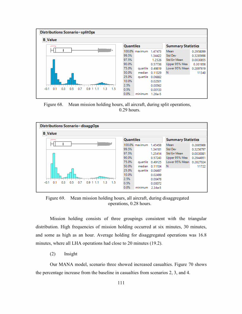
111

Figure 68. Mean mission holding hours, all aircraft, during split operations,

0.29 hours.

Figure 69. Mean mission holding hours, all aircraft, during disaggregated

operations, 0.28 hours.

Mission holding consists of three groupings consistent with the triangular

distribution. High frequencies of mission holding occurred at six minutes, 30 minutes,

and some as high as an hour. Average holding for disaggregated operations was 16.8

minutes, where all LHA operations had close to 20 minutes (19.2).

(2) Insight

Our MANA model, scenario three showed increased casualties. Figure 70 shows

the percentage increase from the baseline in casualties from scenarios 2, 3, and 4.

112

Figure 70. STOM-V graph of increased casualties with scenario 3.

Aviation insight about increased casualties from dismounted infantry.

Operationally, it is almost always planned for to hold after inserting infantry for

contingencies such as CASEVAC/MEDEVAC and emergency extract (Team

Expeditionary & Cohort 311-132, 2014). The amount of holding generated by the Simio

model is a best case. Calculations here, however, will only account for holding associated

with the launch of aircraft and should be seen as the lowest total savings.

Spreadsheet calculations are made to transform holding data into potential savings

in energy and money. First, we combine average mission holding and burn rates for the

principal drivers of energy the MV-22 and CH-53. We look at just these two platforms

because the F-35B does not join the MEU until it sails and this research wishes to

incorporate energy savings during the length workup period.

113

Table 8. The top line has all LHA, split, and disaggregated operations. Below are the low, operational planning, and high end burn rates in one table (i.e.,

“lo,” ”Planning,” and “hi”). These numbers provide a range for a decision maker.

Another calculation is made to convert mission holding (hours) and burn rate

(lbs/hr) in to pounds of fuel burned per mission. Figure 71 shows pounds of fuel burned

from the three scenarios at three potential levels.

Figure 71. The bar graph shows pounds of fuel burned per sortie. A sortie is

defined as one hour of flight launched from a ship.

Thus, the combined assault mission holding fuel for both the MV-22 and the CH-

53K can be calculated. For the six-month workup period, there are eight long-range raids

given for a MEU, which either has a low, operational planning, or high number of raids.

After raids done for training on workups, there are additional “real-world” raids

complete. For the six-month MEU deployment, we look at three levels of deployment

ALL “LHA” “Split” “Disaggregated”

Mean Holding (hrs) 0.328 0.295 0.288 Low (lo) Planning High (Hi)

Burn Rate MV-22 2,500 3,200 4,700 pounds/hour (lbs/hr)

Burn Rate CH-53K 2,900 3,600 4,900 lbs/hr

114

intensity consisting of 6-, 24-, or 48-raid missions. Figure 72 shows the impact of assault

mission holding for the MEU based on deployment intensity.

Figure 72. Assault aircraft on a MEU deployment at three levels of deployment

intensity consisting of 6-, 24-, or 48-raid missions.

For the purpose of this research a mission is a long range raid. Workups consist of

two missions for each at sea training period prior to the actual deployment. With four

training periods (e.g., certification exercise [CERTEX]), eight missions are added in with

whether the MEU is conducting a mission every month, week, or twice a week. Figure 73

shows the money saved after 10 years of operating either split or disaggregated. To

convert the mission holding fuel to dollars, again we use spreadsheet calculators.

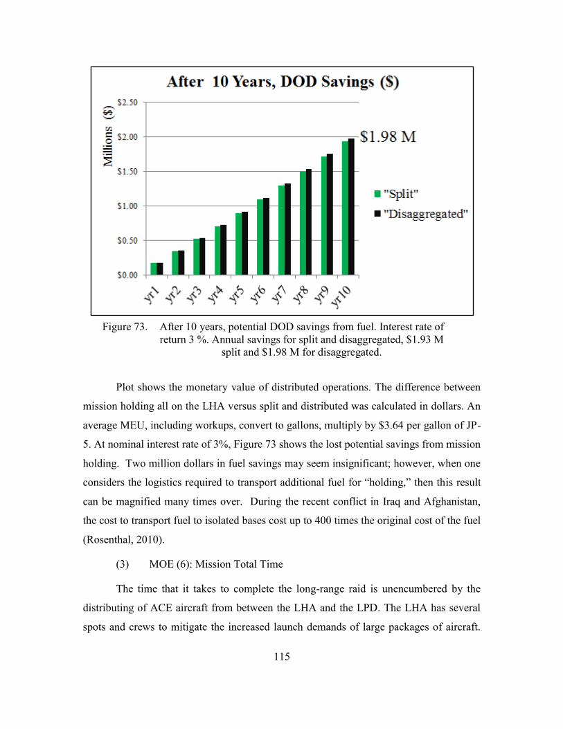
115

Figure 73. After 10 years, potential DOD savings from fuel. Interest rate of

return 3 %. Annual savings for split and disaggregated, $1.93 M split and $1.98 M for disaggregated.

Plot shows the monetary value of distributed operations. The difference between

mission holding all on the LHA versus split and distributed was calculated in dollars. An

average MEU, including workups, convert to gallons, multiply by $3.64 per gallon of JP-

5. At nominal interest rate of 3%, Figure 73 shows the lost potential savings from mission

holding. Two million dollars in fuel savings may seem insignificant; however, when one

considers the logistics required to transport additional fuel for “holding,” then this result

can be magnified many times over. During the recent conflict in Iraq and Afghanistan,

the cost to transport fuel to isolated bases cost up to 400 times the original cost of the fuel

(Rosenthal, 2010).

(3) MOE (6): Mission Total Time

The time that it takes to complete the long-range raid is unencumbered by the

distributing of ACE aircraft from between the LHA and the LPD. The LHA has several

spots and crews to mitigate the increased launch demands of large packages of aircraft.

116

As previously described we made the LHA worst case with regard to spot availability,

restricting total numbers of spots and crews for the LHA.

Figure 74. After 1,000 replications, practically no significant effect on mission

time.

(4) Conclusions

Multiple air capable ships mitigate the risk of any one platform fouling an entire

operation. Distributing forces on many platforms may be cheaper from smaller less

complex systems and provide numerous redundant parts. Total mission times may be

reduced by positioning air capable ships closer to the objective. There was no change to

total mission time from distributed operations, however, a change in operating procedures

may decrease mission holding, which might translate into significant monetary savings.

117

VII. CONCLUSIONS AND RECOMMENDATIONS

Americans can always refuse to pay the price for maintaining an amphibious capability, thereby giving up what Liddell Hart calls “the greatest strategic asset that a sea-based power possesses.” If Americans should choose to take such a step, they will have, in effect, accomplished what no enemy has managed to do: defeat a modern amphibious operation

—Col Theodore L. Gatchel, USMC (Ret)

This research develops a two-stage model, where we found the most important

factor to be speed. While this model is by no means the end-all, it provides verification

and validation for other ACVs, SSCs, AAV upgrades, and amphibious operation models.

This research supports operationally effective ACVs that operate at speeds much less

than 40 or even 30 mph. These speeds align closely with the M1A1 tank land speed, and

are often cited as the top U.S. capability that any future amphibian must meet. The vision

for the future amphibious fleet has vehicles launching from ranges of 25 nm, 12 nm, and

5 nm off shore. Speeds, ranges, and quantities of SSCs were all varied in an efficient

DOE to better understand the complex trade-space of amphibious assault.

A. OVERVIEW

In the aftermath of the EFV, the Marine Corps identified a new top acquisition

priority in the ACV, which is a wheeled, amphibian designed with lessons learned from

more than 13 years of combat operations. Even with an increasingly fiscally constrained

force, the vehicle of complementary platforms of SSC must bring Marines to objectives

quickly and safely. Currently, there are four prototypes being tested. This research uses

agent-based and discrete-event simulation modeling, combined with a state-of-the-art,

nearly orthogonal-and-balanced DOE to model an end-to-end amphibious assault. An

overview of the model-test-model approach is provided in Appendix J.

118

B. ENERGY INSIGHTS

This research builds on previous SE graduate-level work that found advanced

platforms like the MV-22 and CH-53K embarked with Marines provide great capacity,

yet consume great quantities of fuel. This research models a long-range raid complete

with MV-22s and CH-53Ks, which is one of the most taxing evolutions for not only the

deck cycle, but for the ACE. The DES in Simio within this document shows the benefit to

split and disaggregated operations. Specifically, operating procedures exist that may

reduce mission holding and can be done in a way with no effect on total mission time.

Meanwhile, several analytical methods and the MANA simulation show that the ACV,

AAV, and the next SSC should be designed to meet the following specifications:

ACV speed: 16 kts/18 mph

ACV debark distances of 5 nm and 12 nm

LCAC quantities should be greater than two or have operating speeds > 44 kts

In summary:

A disaggregated and split operation is one way to mitigate excessive mission holding.

The SSC, ACV, and the AAV upgrade need not be as fast as a tank is on land in order to be mission effective and meet requirements.

C. OPERATIONAL INSIGHTS

The ability to conduct STOM-V and STOM-S in a variety of ways allows for a

landing to quickly mass forces and support ashore. During an amphibious assault, the

defending force has an advantage of concealment and artillery, yet the attack can choose

the time and place to land to select an advantageous avenue of approach. Operationally,

SSCs have consisted of AAVs that capably brought many Marines ashore to Kuwait.

Having amphibious vehicles allows for river and canal crossings, as was the case in Iraq.

This is not, however, an opposed landing. During an amphibious assault vice an

amphibious landing, a bigger force is required. More armor is required to defend the

landing force against the variety of weapons that can be brought to bear during the

launch, swimming, transition through the surf, and movement inland—all of which

119

cannot happen slowly. Heavily armored vehicles that might hold more may also have

decreased performance and be vulnerable, compared to medium-sized ACVs.

This research also looks at the MEU contribution from nonamphibious assault

landings, when forces are brought in to a secure landing zone. Figure 75 shows Blue and

Red casualties by scenario.

Figure 75. What is the most important vehicle type in an amphibious assault?

Of the four scenarios, scenario 3 masses Blue force the fastest with the MV-22; however, dismounted infantry are not afforded the same

protection as those inside vehicles like the ACV and AAV.

To give this research the pedigree of a traceable scenario, the author uses EW 12.

Two ACVs will carry a reinforced squad, which means that with ACVs, Marines will

have twice the firepower with two RWSs, as opposed to one on the legacy AAV tractor.

Nevertheless, the affect from a self-deploying amphibious vehicle is a single wave, which

masses firepower ashore without paying the price of being a serial in a wave of SSCs.

120

1. MOE Insights

Blue casualties are fewer when just connectors and an autonomous AAV wave are

used. Blue casualties increase when Marines are dismounted early as with the STOM-V.

An MV-22 long-range raid does increase Red casualties and the times that Blue attrites

Red to one-third their strength. Red casualties depend on ACV speed, debark distance,

LCAC quantity, and LCAC speed. The LCAC is the SSC. Time increases with distance;

however, the benefit in going from three to four LCACs is not as great as the benefit in

going from two to three. Depending on the size of the force, there are diminishing returns

with the arrival of additional LCACs. Here, the fourth LCAC had a negligible impact,

save functioning as a reserve for the other three.

D. FUTURE RESEARCH

The Marine Corps and DOD have many highly useful spreadsheet tools and

calculators for specific needs. Before creating another, this author suggests asking, “What

is not being modeled because it is too complex?” and then making an attempt to model it.

Future work includes exploring the metamodels from this simulation in a future decision

tool that shows operational energy and operational effectiveness. This analysis was broad

and much can be done to refine it, such as:

Impacts of terrain. Adjusting the RGB terrain file at the water’s edge from water, to surf, to shore, and then inland.

Increased fidelity in the transition through an active surf.

Increased ranges and lethality of Red forces.

A reduced signature offload of ACVs.

Applying methods from Chapter V to: MLP launch of LCAC, LCAC launch of ACV, ACV dismount of infantry.

Impact of mobile artillery.

Increased constraints on the well deck of the LHA/LHD.

Egress from the ACV; exploring how best to employ a reinforced squad of Marines split between two ACV vehicles.

121

E. SUMMARY

Complex spreadsheet tools, with thousands of lines of VBA, are less adaptive than object-oriented models.

This research modeled over 100 agents and 75 factors.

The LCAC, ACV, AAV, and MV-22 all are distributed systems, but it was a self-deployer that provided the desired affect against an enemy in the defense.

Speed, though highly influential, need not be at top capability to be effective.

Two million dollars in fuel savings may seem insignificant; however, when one considers the logistics required to transport additional fuel for “holding,” then this result could be magnified many times over.

The force that responds to the next crisis or contingency will be the force that is

closest to it—the Marine Expeditionary Units (MEUs) embarked on ships. This research

is leaning forward by making a first attempt at modeling an end-to-end amphibious

assault. In hundreds of thousands of simulated amphibious assaults, we observe the trade-

space formed by the many complex parameters considered when employing concept

complementary platforms of surface and vertical ship-to-objective-maneuver. In the end,

we realize quantifiable values that maximize mission effectiveness and better inform the

top procurement priorities for the United States Naval forces.

122


123

APPENDIX A. COMPLETE TABLE OF BLUE SQUADS

Table 9. Complete table of the 113 Blue squads in MANA. Squad Number Squad Parent

Number of Agents

Agent Class Number

Run Start Delay

1 LHD None 1 99 0

2 LPD-19 None 1 99 0 3 LSD-41 None 1 99 0

4 LCAC-1-1 3 1 88 430

5 LCAC-2-1 3 1 88 430

6 LCAC-3-1 3 1 88 430

73 LCAC-4-1 3 1 88 430

7 LCAC-1-2 3 1 88 4720

8 LCAC-2-2 3 1 88 4720

9 LCAC-3-2 3 1 88 4720

74 LCAC-4-2 3 1 88 4720

10 LCAC-1-3 3 1 88 9010

11 LCAC-2-3 3 1 88 9010

12 LCAC-3-3 3 1 88 9010

13 LCAC-1-4 (NOT ACTIVE) 3 1 88



75 LCAC-4-3 3 1 88 9010

34 M1A1-1 4 1 2 0

35 M1A1-2 5 1 2 0

36 M1A1-3 7 1 2 0

37 M1A1-4 8 1 2 0

76 ACV-P-1 6 1 4 0

77 ACV-P-2 6 1 4 0

78 ACV-P-3 6 1 4 0

79 ACV-P-4 73 1 4 0

80 ACV-P-5 73 1 4 0

81 ACV-P-6 73 1 4 0

82 ACV-P-7 75 1 4 0 83 ACV-P-8 9 1 4 0

84 ACV-P-9 9 1 4 0

85 ACV-P-10 9 1 4 0

86 ACV-P-11 74 1 4 0

87 ACV-P-12 74 1 4 0

88 ACV-P-13 74 1 4 0

124

Squad Number Squad Parent

Number of Agents

Agent Class Number

Run Start Delay

89 ACV-P-14 74 1 4 0

90 ACV-P-15 12 1 4 0

91 ACV-P-16 12 1 4 0

92 ACV-P-17 75 1 4 0

93 ACV-R-1 6 1 4 0

94 ACV-C-1 73 1 4 0

50 Inf-1 76 3 1 0 51 Inf-2 77 3 1 0 52 Inf-3 78 3 1 0 53 Inf-4 79 3 1 0 54 Inf-5 80 3 1 0 55 Inf-6 81 3 1 0 56 Inf-7 82 3 1 0

57 Inf-8 83 3 1 0 58 Inf-9 84 3 1 0 59 Inf-10 85 3 1 0 60 Inf-11 86 3 1 0 61 Inf-12 87 3 1 0 62 Inf-13 88 3 1 0

63 Inf-14 89 3 1 0

64 Inf-15 90 3 1 0 65 Inf-16 91 3 1 0

66 Inf-17 92 3 1 0 67 Inf-18 93 3 1 0

95 Inf-19 94 3 1 0 96 Inf-20 25 3 1 0

97 Inf-21 26 3 1 0

98 Inf-22 27 3 1 0

99 Inf-23 28 3 1 0

100 Inf-24 29 3 1 0 101 Inf-25 30 3 1 0 102 Inf-26 31 3 1 0 103 Inf-27 32 3 1 0

104 Inf-28 33 3 1 0

105 Inf-29 16 3 1 0

106 Inf-30 17 3 1 0

107 Inf-31 18 3 1 0

108 Inf-32 19 3 1 0 109 Inf-33 20 3 1 0 110 Inf-34 21 3 1 0 111 Inf-35 22 3 1 0 112 Inf-36 23 3 1 0 113 Inf-37 24 3 1 0

125

APPENDIX B. FER BY SCENARIO WITH THE RAW OUTPUT DATA

Figure 76. Shows the FER, by scenario, with the non-collapsed data.

126


127

APPENDIX C. COLLAPSED DATA BY SCENARIO, PAIRED

Figure 77. One-way analysis of mean “Red casualties” MOE by scenario.

128


129

APPENDIX D. RAW OUTPUT DATA, PAIRED

Figure 78. One-way analysis of the mean “Red casualties” MOE by scenario

with the non-collapsed output data.

130


131

APPENDIX E. MULTIPLE LINEAR REGRESSION COMPARISON TABLE

Figure 80. MOE “Blue casualties” actual by predicted, summary of fit,

prediction profiler, and Pareto plots.

132

Figure 81. MOE “Red casualties” summary of fit, sorted parameter estimates,

prediction profiler, and Pareto plots.

Response Mean(AIIeg2Cas.Red)

Actual by Predicted Plot

2 4 8 10 12 14 16 18202224262830 Mean(AIIeg2Cas.Red.) Predicted P<.OOOl

RSq=0 .48 RMSE=5.2705

Summary of Fit RSquare 0 .480168 RSquare Adj 0 .476588 Root Mean Square Error 5.270466 Mean of Response 23.36517 Observat ions (or Sum Wgts) 2048

Analysis of Variance Sum of

Sou.-ce OF Squares Mean Squar-e FRatto Model 14 52163AO 3725.96 134 .1343 Error 20 33 56472.29 27.78 Pmb > F

C. Total 2047 108635.69 <.0001*

Sorted Parameter Estimates

Term Estimate Std Error LCDbk!Ji, t125· 12] · 10 .28631 0 .50422 ACVMvtSpd 0 .1933118 0 .0 10966 LCDbkDi,;t[25· 12]• LCACQty(3· 2 8 .1278321 0 .697515 Scenario [l ] · 2 .196354 0.201718 Scenario[2] 1.8155599 0 .201718 Scenario[3] · 1.553841 0 .201718 RedlnfCisRng 0 .0001235 1.614e-5 Sceoa,io [1]'(ACVMvtSpd· 26.5) 0 .1266342 0 .0 1884 Scena,io [2J• [ACVMvtSpd· 26.5) ·0 .105782 0 .01884 LCDbkDi,;t[1 2 · 5] · 2 .314m 0 .424185 Sceoa, io [3]• [ACVMvtSpd·26.5) 0 .0933938 0 .0 1884 LCDbkDi,tl12 · 5]•LCACQty[3·2] 1.6942506 0 .486529 LCDbkDi,t (12 · 5]•LCACQty[4 · 3] 1.0103107 0 .471621 LCDbklli,t125· 12]• LCACQty!4· 3 1.3062766 0 .675271

Prediction Profiler

·-==~~u==::l Pwb>l•l I~ <.OOOl* <.0001 <.OOOl* <.OOOl* <.0001 .. <.OOOl* <.OOOl* <.OOOl* <.OOOl* <.OOOl* <.OOOl* o.ooo5· 0 .0323"

0 .0532

j {)\':= 1~ x-- :--r~~ 1° 1 ~ b~b~b~b~ 6.!-.b.!...b~.b.:.. I I I ~ ~ ~ ~ I I ~ ~.-~r-.~~~~ ~!£§~~~~

Effect Screening

26.5

ACVMvtSpd

12501

RedlnfCisRng

Pareto Plot o f Transformed Estimates

Term LCDbkDi,;t[12· 5]•LCACQty[3· 2] ACVMvt5pd LCDbkDi,;t[25· 12] LCDbkDi,;t[25·12]• LCACQty(3·2 Scenario[l ] LCDbkDi,;t[12·5] RedlnfCisRng

Orthog

Scenano[1]•[ACVMvtSpd· 26.5) 0 .9 11825

Scenario[l ] ·0 .897111 Scenario[2] LCDbkDi,;t[12 · 5]•LCACQty[4 · 3] Scenario[3]•[ACVMvt5pd· 26.5) Scenario [2]• [ACVMvtSpd·26.5) LCDbkDi,;t[25 · 12]•LCACQty!4· 3

Scena rio LCDbkDi,;t

2

LCACQty

133

Figure 82. MOE “time” summary of fit, sorted parameter estimates, prediction

profiler, and Pareto plots.

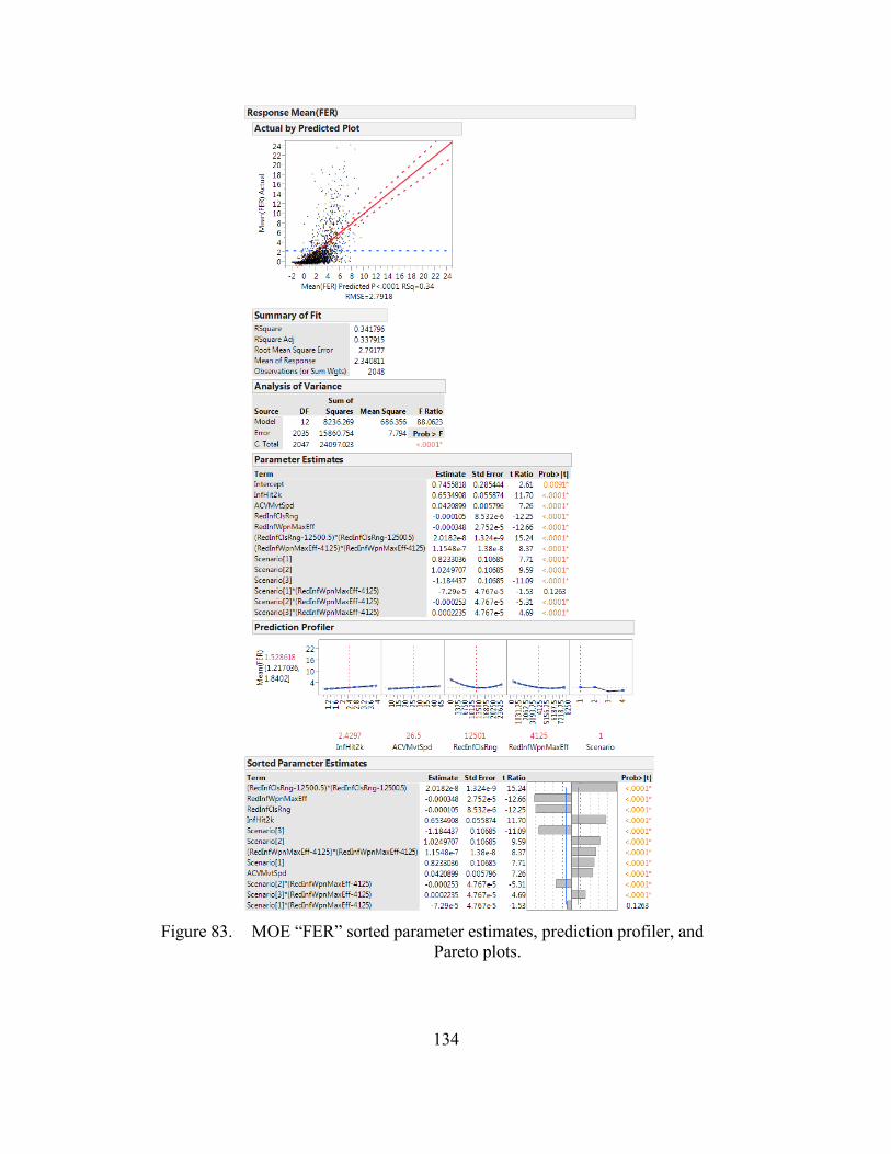
134

Figure 83. MOE “FER” sorted parameter estimates, prediction profiler, and

Pareto plots.

135

APPENDIX F. “TIME” MOE, MULTIPLE LINEAR REGRESSION, ASSUMPTIONS

Figure 84. MOE “time” advanced regression model, normal Q-Q plot, closely

fits along the line, passes the “fat pencil test.”

136


137

APPENDIX G. ALL 77 MIXED (CONTINUOUS AND DISCRETE) FACTORS

Figure 86. Complete NOB, 77 factor DOE.

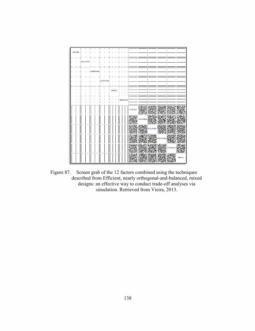
138

Figure 87. Screen grab of the 12 factors combined using the techniques

described from Efficient, nearly orthogonal-and-balanced, mixed designs: an effective way to conduct trade-off analyses via

simulation. Retrieved from Vieira, 2013.

139

APPENDIX H. MEANS COMPARISON USING STUDENT T-TEST

Figure 88. T Means comparison for statistically significant scenarios using

student t-Test.

140

Figure 89. Paired comparison, scenarios two and four for statistical significance

141

APPENDIX I. SIMIO AND MANA DASHBOARD COMPARISON

Figure 90. Screen shot of Simio dashboard

Figure 91. Screen shot of terrain billboard in MANA.

142


143

APPENDIX J. APPROACH, MODEL-TEST-MODEL

Figure 92. An illustration of the model-test-model approach, see chapter III for actual concept of operations and scenario development.

144


145

LIST OF REFERENCES

15th Marine Expeditionary Unit. (2012). 15th Marine Expeditionary Unit History. Retrieved from http://www.15thmeu.marines.mil/About/History.aspx

Achterling, M. (2014). U.S. Navy photo by Mass Communication Specialist, 2nd Class, Michael Achterling. Retrieved from http://www.ctf76.navy.mil/gallery/2014/apr/apr.htm

Axe, D. (2012). Inside the Army’s doomed quest for the ‘perfect’ radio. Wired. Retrieved from http://www.publicintegrity.org/2012/01/10/7816/failure-communicate-inside-armys-doomed-quest-perfect-radio

Besser, J., Hobbs, J., Hovis, K., Hunter, D., Leaman, B., McPherson, J., . . . Valliere, E. (2013). Expeditionary energy efficiency in support of foreign humanitarian aid/disaster relief (Capstone Report). Monterey, CA: Naval Postgraduate School.

Charette, R. N. (2008). What’s wrong with weapons acquisitions? Spectrum, IEEE, 45(11), 33–39.

Cioppa, T. M., Lucas, T. W., & Sanchez, S. M. (2004). Military applications of agent-based simulations. Proceedings of the 2004 Winter Simulation Conference (pp. 171–180). Piscataway, NJ: IEEE.

Dempsey, M. E. (2012). Joint operational access concept (JOAC). Washington, D.C.: Department of Defense.

Department of Defense. (1992). 3–02. Joint doctrine for amphibious operations. Washington, D.C.: Department of Defense.

Department of the Navy. (1998). MCDP 3: Expeditionary operations. Washington, D.C.: Department of Defense.

Department of the Navy. (2007, October 15). Seabase to shore connector analysis of alternatives final report. Retrieved from https://cle.nps.edu/access/content/group/72686d99-7c35-4290-9670-260641f1f0f0/Lesson%2014%20Case%207%3A%20SSC/SSC_AoA_Report.pdf

Edwards, E. (1868). The life of Sir Walter Raleigh: Based on contemporary documents... Together with his letters; Now first collected. I (Vol. 2). Macmillan. London, United Kingdom.

Eckstein, M. (2015, March 11). Marines may merge ACV increments as industry chases higher requirements. Retrieved from http://news.usni.org/2015/03/11/marines-may-merge-acv-increments-as-industry-chases-higher-requirements

146

Feickert, A. (2013, June). Marine Corps amphibious combat vehicle (ACV) and Marine personnel carrier (MPC): Background and issues for Congress. Retrieved from http://www.fas.org/sgp/crs/weapons/R42723.pdf

Fuentes, G. (2015, March 10). Picture of MV-22 nacels and Ground Combat Element (GCE), pilot program forges bonds between Marines and U.S. Special Operations Forces. The USNI News. Volume I, issue I, p. 1-5. Retrieved from http://news.usni.org/2015/03/10/pilot-program-forges-bonds-between-marines-and-u-s-special-operations-forces

Galante, A. (2009). USS ‘Wasp’ (LD1) com Ospreys. Retrieved from http://www.naval.com.br/blog/2009/07/22/uss-wasp-lhd-1-com-ospreys/

Gatchel, T. (1996). At the water’s edge: Defending against the modern amphibious assault. Annapolis, MD: Naval Institute Press.

Griffith, S. (1971). The art of war. London: Oxford University Press.

Heinl, R. D. (1966). Dictionary of military and naval quotations. Naval Institute Press.

Hoe, K. J. (2001). An analysis of distributed combat systems (Master’s thesis). Monterey, CA: Naval Postgraduate School.

Howard, M., Paret, P., & West, R. (1984). Carl Von Clausewitz: On war. Princeton, NJ: Princeton University Press.

Hughes, W. P. (2015). The U.S. Naval Institute on naval tactics (2nd ed.). The U.S. Naval Institute. Annapolis, MD.

Kelton, W. D., Smith, J. S., & Sturrock, D. T. (2011). Simio & simulation: Modeling, analysis, applications. Learning Solutions. Boston, MA.

LaGrone, S. (2015, February). WEST: Marines plan to issue amphibious combat vehicle request for proposal in March. The USNI News. Retrieved from http://news.usni.org/2015/02/12/west-marines-plan-issue-amphibious-combat-vehicle-request-proposal-march

Langworth, R. (2008). Churchill by himself: The definitive collection of quotations. Public Affairs, New York. p. 576.

Lucas, T. (2014). Lecture notes in statistics class: Hypothesis testing (OA 3102 Statistics). Naval Postgraduate School, Monterey, CA. Retrieved from https://cle.nps.edu/access/content/group/4235b6f3-d2c1-4c6d-b26c-0b9de11575d3/Lecture%20slides/Hypothesis%20Testing.pdf

Marine Corps Expeditionary Energy Office (E2O). (2012). Retrieved from http://www.hqmc.marines.mil/e2o/E2OHome/AboutUs.aspx

147

McIntosh, G., Galligan, D., Anderson, M. A., & Lauren, M. K. (2007). MANA-V (Map Aware Non-uniform Automata-Vector) supplementary manual. Defense Technology Agency. New Zealand

Obama, B. (2011, October 21). Remarks by the President on ending the war in Iraq. White House, Washington, D.C.

Patton, G. S., & Harkins, P. D. (1995). War as I knew it. Houghton Mifflin Harcourt.

Sanchez, S. M. (1994, December). A robust design tutorial. Proceedings of the 1994 Winter Simulation Conference (pp. 106–113). Piscataway, NJ: IEEE.

Sanchez, S. M. (2007). Work smarter, not harder: Guidelines for designing simulation experiments. Proceedings of the 2007 Winter Simulation Conference (pp. 84–94). doi:10.1109/WSC.2007.4419591. Piscataway, NJ: IEEE.

Sanchez, S. M., Sánchez, P. J., & Wan, H. (2014, July). Simulation experiments: Better insights by design. Proceedings of the 2014 Summer Simulation Multiconference (p. 53). Society for Computer Simulation International.

Simio LLC. (2010). Introduction to Simio. Pittsburgh, PA. Retrieved from http://www.Simio.com/about-Simio

Skahen, S., Benner, S., Boyett, M., Brookhart, M., & Kure, J. (2013). Exploring the reduction of fuel consumption for ship-to-shore connectors of the Marine Expeditionary Brigade (Capstone Report). Monterey, CA: Naval Postgraduate School.

Smith, S. M. (2013). U.S. Marine Corps MV-22 Osprey tiltrotor aircraft prepare to take off from the amphibious transport dock ship USS Mesa Verde (LPD 19) in the Atlantic Ocean December 14, 2013. Retrieved from http://commons.wikimedia.org/wiki/File:U.S._Marine_Corps_MV-22_Osprey_tiltrotor_aircraft_prepare_to_take_off_from_the_amphibious_transport_dock_ship_USS_Mesa_Verde_(LPD_19)_in_the_Atlantic_Ocean_Dec._14,_2013_131214-N-BD629-087.jpg

Suite of Analytics Software (SAS). (2014). JMP 11 online documentation. Retrieved from http://www.jmp.com/support/help

Taguchi, G. (1986). Introduction to quality engineering: Designing quality into products and processes. Tokyo: The Organization.

Team Expeditionary & Cohort 311-132. (2014). Operational energy/operational effectiveness investigation for scalable Marine Expeditionary Brigade forces in contingency response scenarios (Master’s thesis). Monterey, CA: Naval Postgraduate School. Retrieved from https://cle.nps.edu/xsl-portal/tool/b0d2a28e-bff7-451b-b663-cfd03543d98f/posts/downloadAttach/73963.page

148

Trickey, W. R., Benbow, R. C., & Taylor, D. G. (2010). MEB capabilities study. Alexandria, VA: Center for Naval Analyses.

Unit of Action Maneuver Battle Lab (UAMBL). (2003) Operational requirements document (ORD) for the future combat systems, Fort Knox, KY: UAMBL. Retrieved from http://www.rand.org/content/dam/rand/pubs/monographs/2012/ RAND_MG1206.pdf

U.S. History. (2015). History of the U.S. Marine Corps Chronology. Retrieved from http://www.u-s-history.com/pages/h3795.html

U.S. Marine Corps. (1998). MCDP 3–Expeditionary operations. Washington, D.C.: Department of Defense.

U.S. Naval War College. (2015). The U.S. Naval War College at the Naval Postgraduate School Course Syllabus. Naval Postgraduate School, Monterey, CA. Retrieved from https://cle.nps.edu/xsl-portal/site/73952c7b-5692-4df5-970a-8aee9260d22d/ page/61a4e4ab-4095-4dcd-a0e7-6da0e6985ca9

Vieira, Jr., H., Sanchez, S. M., Kienitz, K. H., & Belderrain, M. C. M. (2011, December). Improved efficient, nearly orthogonal, nearly balanced mixed designs. Proceedings of the 2011 Winter Simulation Conference (pp. 3600–3611). Piscataway, NJ: IEEE.

Vieira, Jr., H., Sanchez, S. M., Kienitz, K. H., & Belderrain, M. C. M. (2013). Efficient, nearly orthogonal-and-balanced, mixed designs: An effective way to conduct trade-off analyses via simulation. Journal of Simulation (7: 264-275). (Special Issue on Input/Output Analysis).

Wackerly, D., Mendenhall, W., & Scheaffer, R. (2008). Mathematical statistics with applications. Cengage Learning.Belmont, CA.

Wargaming Division. (2012). Expeditionary Warrior 2012 (EW 12) Final Report 23 July 2012, Wargaming Division, Marine Corps Warfighting Laboratory, Retrieved from http://www.defenseinnovationmarketplace.mil/resources/Marine_Corps_ War_Game.pdf

149

INITIAL DISTRIBUTION LIST

1. Defense Technical Information Center Ft. Belvoir, Virginia 2. Dudley Knox Library Naval Postgraduate School Monterey, California

naval postgraduate school - apps.dtic.mil · it identifies ttps and mission profiles that achieve...

Documents