naval postgraduate school - defense technical …dtic.mil/dtic/tr/fulltext/u2/a514229.pdf · and...

NAVAL

POSTGRADUATE SCHOOL

MONTEREY, CALIFORNIA

THESIS

Approved for public release; distribution is unlimited

STATE-SPACE MODELING, SYSTEM IDENTIFICATION AND CONTROL OF A 4th ORDER ROTATIONAL

MECHANICAL SYSTEM

by

Jeremiah P. Anderson

December 2009

Thesis Advisor: Xiaoping Yun Second Reader: Alex Julian

i

REPORT DOCUMENTATION PAGE Form Approved OMB No. 0704-0188 Public reporting burden for this collection of information is estimated to average 1 hour per response, including the time for reviewing instruction, searching existing data sources, gathering and maintaining the data needed, and completing and reviewing the collection of information. Send comments regarding this burden estimate or any other aspect of this collection of information, including suggestions for reducing this burden, to Washington headquarters Services, Directorate for Information Operations and Reports, 1215 Jefferson Davis Highway, Suite 1204, Arlington, VA 22202-4302, and to the Office of Management and Budget, Paperwork Reduction Project (0704-0188) Washington DC 20503. 1. AGENCY USE ONLY (Leave blank)

2. REPORT DATE December 2009

3. REPORT TYPE AND DATES COVERED Master’s Thesis

4. TITLE AND SUBTITLE State-space Modeling, System Identification and Control of a 4th Order Rotational Mechanical System 6. AUTHOR(S) Jeremiah P. Anderson

5. FUNDING NUMBERS

7. PERFORMING ORGANIZATION NAME(S) AND ADDRESS(ES) Naval Postgraduate School Monterey, CA 93943-5000

8. PERFORMING ORGANIZATION REPORT NUMBER

9. SPONSORING /MONITORING AGENCY NAME(S) AND ADDRESS(ES) N/A

10. SPONSORING/MONITORING AGENCY REPORT NUMBER

11. SUPPLEMENTARY NOTES The views expressed in this thesis are those of the author and do not reflect the official policy or position of the Department of Defense or the U.S. Government. 12a. DISTRIBUTION / AVAILABILITY STATEMENT Approved for public release; distribution is unlimited

12b. DISTRIBUTION CODE

13. ABSTRACT (maximum 200 words) In this thesis, a 4th order rotational mechanical plant provided by Educational Control Products is modeled from first principles and represented in state-space form. Identification of the state-space parameters was accomplished using the parameter estimation function in Matlab’s System Identification Toolbox utilizing experimental input/output data. The identified model was then constructed in Simulink and the accuracy of the identified model parameters was studied. The open loop stability of the plant, as well as its controllability and observability were analyzed to determine the applicability of a pole placement control strategy. Based on the results of this analysis, a full state variable feedback controller was investigated to place the system’s poles such that a rotational disk would perfectly track a step angle input with less than five percent overshoot and have less than a one second settling time, with no steady-state error. A refinement of this controller, to include an observer to estimate the system states, was also investigated. Finally, the results of this work are summarized and presented as a series of laboratories applicable to a course in state-space design.

15. NUMBER OF PAGES

117

14. SUBJECT TERMS System Identification, State-space, Pole Placement, Full State Feedback, Observer

16. PRICE CODE

17. SECURITY CLASSIFICATION OF REPORT

Unclassified

18. SECURITY CLASSIFICATION OF THIS PAGE

Unclassified

19. SECURITY CLASSIFICATION OF ABSTRACT

Unclassified

20. LIMITATION OF ABSTRACT

UU NSN 7540-01-280-5500 Standard Form 298 (Rev. 8-98) Prescribed by ANSI Std. Z39.18

ii

THIS PAGE INTENTIONALLY LEFT BLANK

iii

Approved for public release; distribution is unlimited

STATE-SPACE MODELING, SYSTEM IDENTIFICATION AND CONTROL OF A 4th ORDER ROTATIONAL MECHANICAL SYSTEM

Jeremiah P. Anderson Lieutenant, United States Navy

B.S., University of California, Los Angeles, 2002

Submitted in partial fulfillment of the requirements for the degree of

MASTER OF SCIENCE IN ELECTRICAL ENGINEERING

from the

NAVAL POSTGRADUATE SCHOOL DECEMBER 2009

Author: Jeremiah P. Anderson

Approved by: Xiaoping Yun Thesis Advisor

Alex Julian Second Reader

Jeffrey B. Knorr Chairman, Department of Electrical and Computer Engineering

iv


v

ABSTRACT

In this thesis, a 4th order rotational mechanical plant provided by

Educational Control Products is modeled from first principles and represented in

state-space form. Identification of the state-space parameters was accomplished

using the parameter estimation function in Matlab’s System Identification Toolbox

utilizing experimental input/output data. The identified model was then

constructed in Simulink and the accuracy of the identified model parameters was

studied. The open loop stability of the plant, as well as its controllability and

observability, were analyzed to determine the applicability of a pole placement

control strategy. Based on the results of this analysis, a full state variable

feedback controller was investigated to place the system’s poles such that a

rotational disk would perfectly track a step angle input with less than five percent

overshoot and have less than a one second settling time, with no steady-state

error. A refinement of this controller, to include an observer to estimate the

system states, was also investigated. Finally, the results of this work are

summarized and presented as a series of laboratories applicable to a course in

state-space design.

vi


vii

TABLE OF CONTENTS

I. INTRODUCTION............................................................................................. 1 A. BACKGROUND ................................................................................... 1 B. OBJECTIVE ......................................................................................... 2 C. APPROACH......................................................................................... 3 D. ORGANIZATION.................................................................................. 3

II. STATE-SPACE MODELING OF TORSION PLANT ...................................... 5 A. PLANT AND EQUIVALENT ELECTRICAL MODEL ........................... 5 B. STATE-SPACE MODEL OF SYSTEM................................................. 6 C. SUMMARY........................................................................................... 7

III. MODEL IDENTIFICATION.............................................................................. 9 A. MODELING THE SYSTEM’S DEAD-ZONE......................................... 9 B. SYSTEM IDENTIFICATION VIA PARAMETER ESTIMATION ......... 10

1. System Identification Procedure .......................................... 11 a. Importing Input/Output Data into Matlab .................. 11 b. Constructing Data Structures in Matlab.................... 11 c. Constructing a Continuous-time State-space

Model Object ............................................................... 12 d. Perform Parameter Estimation .................................. 13 e. Extracting the State-space Model.............................. 13

2. Results.................................................................................... 13 C. REDUCED ORDER MODEL.............................................................. 16 D. IDENTIFICATION OF REDUCED ORDER MODEL .......................... 17 E. MODEL VERIFICATION .................................................................... 19 F. SUMMARY......................................................................................... 22

IV. STABILITY, STEADY-STATE ERROR, CONTROLLABILITY AND OBSERVABILITY ......................................................................................... 23 A. STABILITY......................................................................................... 23

1. Calculating Poles of a State-space System......................... 25 2. Stability of Reduced Order Model ........................................ 25

B. STEADY-STATE ERROR .................................................................. 26 C. CONTROLLABILITY.......................................................................... 29

1. Controllability of the 4th Order Model ................................. 30 2. Controllability of the Reduced Order Model........................ 30

D. OBSERVABILITY .............................................................................. 31 1. Observability of the 4th Order Model................................... 32 2. Observability of the Reduced Order Model ......................... 32

E. SUMMARY......................................................................................... 32

V. POLE PLACEMENT DESIGN ...................................................................... 35 A. FULL STATE VARIABLE FEEDBACK ............................................. 35

viii

1. State Feedback Design ......................................................... 36 2. Calculating Feedback Gains................................................. 37 3. Full State Feedback Performance ........................................ 38 4. Correcting Steady-state Error: the Forward Path Gain ...... 40 5. Full State Feedback with Forward Gain Performance ........ 41

B. OBSERVER DESIGN......................................................................... 42 1. Effect of Adding an Observer to the Design........................ 43 2. Calculating the Observer Gains, L ....................................... 44 3. Observer Simulation.............................................................. 45 4. Observer Performance .......................................................... 46

C. SUMMARY......................................................................................... 48

VI. CONCLUSION AND RECOMMENDATIONS............................................... 49 A. CONCLUSIONS................................................................................. 49 B. RECOMMENDATIONS...................................................................... 50

APPENDIX A: STATE-SPACE CONTROL LABORATORIES ............................... 51 A. LAB 1: INTRODUCTION TO MATLAB AND SIMULINK .................. 51 B. LAB 2: SYSTEM IDENTIFICATION................................................... 58 C. LAB 3: MODEL VERIFICATION........................................................ 65 D. LAB 4: STABILITY, CONTROLLABILITY, AND OBSERVABILITY. 67 E. LAB 5: FULL STATE FEEDBACK DESIGN ..................................... 69 F. LAB 6: OBSERVER DESIGN ............................................................ 73

APPENDIX B: MATLAB CODE .............................................................................. 77 MATLAB CODE (LAB 1-6)........................................................................... 77

LIST OF REFERENCES.......................................................................................... 91

INITIAL DISTRIBUTION LIST ................................................................................. 93

ix

LIST OF FIGURES

Figure 1. 4th Order Plant and Electrical/Mechanical Model. ...............................xv Figure 2. Testing the Reduced Order Model..................................................... xvii Figure 3. Final Control Design. ........................................................................ xviii Figure 4. Closed Loop Plant Performance....................................................... xviii Figure 5. Typical Classical Subsystem Control Structure. ................................... 1 Figure 6. 4th Order Torsion Plant. ....................................................................... 2 Figure 7. Plant Setup and Equivalent Electrical Model. ....................................... 6 Figure 8. Extrapolation to Find Dead-zone. ....................................................... 10 Figure 9. Implementation of the Non-linear Dead-zone Block in Simulink. ........ 10 Figure 10. Grey Box Model.................................................................................. 11 Figure 11. Disk 1, 3 Angle using a 0.13V Input.................................................... 15 Figure 12. Reduced Order Plant Model. .............................................................. 16 Figure 13. Experimental Velocity Response to a 0.13 V Input............................. 18 Figure 14. Simulink State-space Plant Model. ..................................................... 19 Figure 15. Comparison of Experimental Response and Model Output................ 19 Figure 16. Verification of Reduced Order Model.................................................. 20 Figure 17. Verification of 4th Order Model. .......................................................... 21 Figure 18. Left Half Plane Poles Time Domain Response................................... 24 Figure 19. Right Half Plane Time Domain Response. ......................................... 24 Figure 20. Standard State-space Model (left); Definition of Error (right).............. 26 Figure 21. Velocity Steady-state Error................................................................. 27 Figure 22. Velocity Response to a 1 Volt Step Input. .......................................... 28 Figure 23. Full State Variable Feedback. ............................................................ 36 Figure 24. Full State Variable Feedback. ............................................................ 38 Figure 25. Implementation of Full State Feedback Control.................................. 38 Figure 26. Step Response of Reduced Plant using State Feedback. .................. 39 Figure 27. Full State Feedback with Forward Path Gain. .................................... 40 Figure 28. State Feedback with Forward Path Gain. ........................................... 41 Figure 29. Step Response of Reduced Order Plant using State Feedback and

Forward Path Gain. ............................................................................ 42 Figure 30. State Feedback using an Observer. ................................................... 43 Figure 31. Final Control Solution. ........................................................................ 46 Figure 32. Comparison of Observer Tracking Performance: (Top: Obs. Poles ~

Same as Closed Loop Poles; Bottom: Obs. Poles 10x larger than Closed Loop Poles). ........................................................................... 47

Figure 33. 2nd Order Plant Model. ...................................................................... 51 Figure 34. Pole Zero Map.................................................................................... 53 Figure 35. Simulink Model Building. .................................................................... 57 Figure 36. 4th Order Plant Model. ....................................................................... 58 Figure 37. Extrapolation to Find Dead-zone. ....................................................... 59 Figure 38. Grey Box Model Identification............................................................. 61

x

Figure 39. Implementing Dead-zone into Model. ................................................. 61 Figure 40. Simulink Model Building. .................................................................... 65 Figure 41. Model Verification. .............................................................................. 66 Figure 42. 4th Order Model.................................................................................. 69 Figure 43. Full State Variable Feedback. ............................................................ 69 Figure 44. Full State Variable Feedback. ............................................................ 71 Figure 45. Plant with State Feedback’s Step Response...................................... 72 Figure 46. Plant with State Feedback and Forward Gain’s Step Response. ....... 72 Figure 47. Graphical Representation of Pole Placement Design using an

Observer............................................................................................. 73 Figure 48. Simulink Implementation of the Controller/Observer. ......................... 75 Figure 49. Observer Convergence for a Sinusoidal Input.................................... 76 Figure 50. Simulation Results.............................................................................. 83 Figure 51. Closed Loop System Response. ........................................................ 89

xi

LIST OF TABLES

Table 1. Required Observer Gains................................................................... 45 Table 2. Table of Common State-space Matlab Commands (After [9]) ............ 55

xii


xiii

LIST OF ACRONYMS AND SYMBOLS

1 3,c c Damping of Disks 1,3

DC Direct Current

1 3,t t

J J Inertia of Entire Disks 1,3

K Feedback Gains

fK Forward Path Gain

bk Back-emf Constant

tk Total Spring Constant

L Observer Gains m-file Matlab file

mO Observability Matrix

p Poles

R Motor Resistance r Reference Input

mT Motor Torque

DT Disk Torque

sT Sampling Time

1,3θ Disk’s Angle

1,3θ& Disk’s Angular Velocity

τ Time Constant

av Applied Voltage

x State Vector

y Measurement

ξ Damping

nω Natural Frequency

%OS Percent Overshoot

xiv


xv

EXECUTIVE SUMMARY

This thesis proposes a state-space approach to model, identify, and

control a 4th order rotational mechanical plant provided by Educational Control

Products (Model 205) shown in Figure 1. This plant consists of a shaft with two

rotational disks, each with their own two masses that are rotated by means of a

DC Servo Motor linked to the shaft by a pulley.

Figure 1. 4th Order Plant and Electrical/Mechanical Model.

The rotational plant was first written in an equivalent free body diagram,

and then first principles were used to derive its equations of motion, and

subsequently represent the plant in state-space form.

11

1 1 1 111 1

33

333 3 3 3

0 1 0 0 01 0

3 30 0 0 1 0

0 0

m m

T T

T T

T T T

PLANTPLANT

b t tT T

a

T T

BA

k k kk J c k J

J R RJ v

k J k J c J

θθθθθθθθ

⎡ ⎤ ⎡ ⎤⎡ ⎤ ⎢ ⎥ ⎡ ⎤ ⎢ ⎥⎛ ⎞⎢ ⎥ ⎢ ⎥ ⎢ ⎥ ⎢ ⎥− − +⎜ ⎟⎢ ⎥ ⎢ ⎥ ⎢ ⎥ ⎢ ⎥= +⎝ ⎠⎢ ⎥ ⎢ ⎥ ⎢ ⎥ ⎢ ⎥⎢ ⎥ ⎢ ⎥ ⎢ ⎥ ⎢ ⎥⎢ ⎥ ⎣ ⎦⎣ ⎦ ⎢ ⎥ ⎢ ⎥− − ⎣ ⎦⎣ ⎦

&

&&&

&

&&&

14243144444444424444444443

(ES.1)

xvi

Identification of the state-space parameters was accomplished using the

parameter estimation function in Matlab’s System Identification Toolbox utilizing

experimental input/output data.

[ ]5

0 1 0 0 01.605 10 .0756 0 0 49.9655

0 1 0 00 0 0 1 00 0 0 0 0

xA B C

−

⎡ ⎤ ⎡ ⎤⎢ ⎥ ⎢ ⎥− −⎢ ⎥ ⎢ ⎥= = =⎢ ⎥ ⎢ ⎥⎢ ⎥ ⎢ ⎥⎣ ⎦ ⎣ ⎦

(ES.2)

Simulation using this structure in Matlab matched well with experimental

input/output data; however, because the structure is rank deficient, it is

subsequently not controllable. Experimental results indicated that the inflexibility

of the shaft connecting the disks meant that the disks acted more as a single

mass turning together than individual parts. In short, modeling the shaft as a

spring has its limitation in the case of an inflexible shaft. The solution devised for

this problem was to use a reduced order model in which the shaft and disks were

modeled as a lump rotating as one. The reduced order model was identified as

0 1 00 .081 52.41 av

θθθθ

⎡ ⎤ ⎡ ⎤ ⎡ ⎤ ⎡ ⎤= +⎢ ⎥ ⎢ ⎥ ⎢ ⎥ ⎢ ⎥−⎣ ⎦ ⎣ ⎦ ⎣ ⎦⎣ ⎦

&

&&& (ES.3)

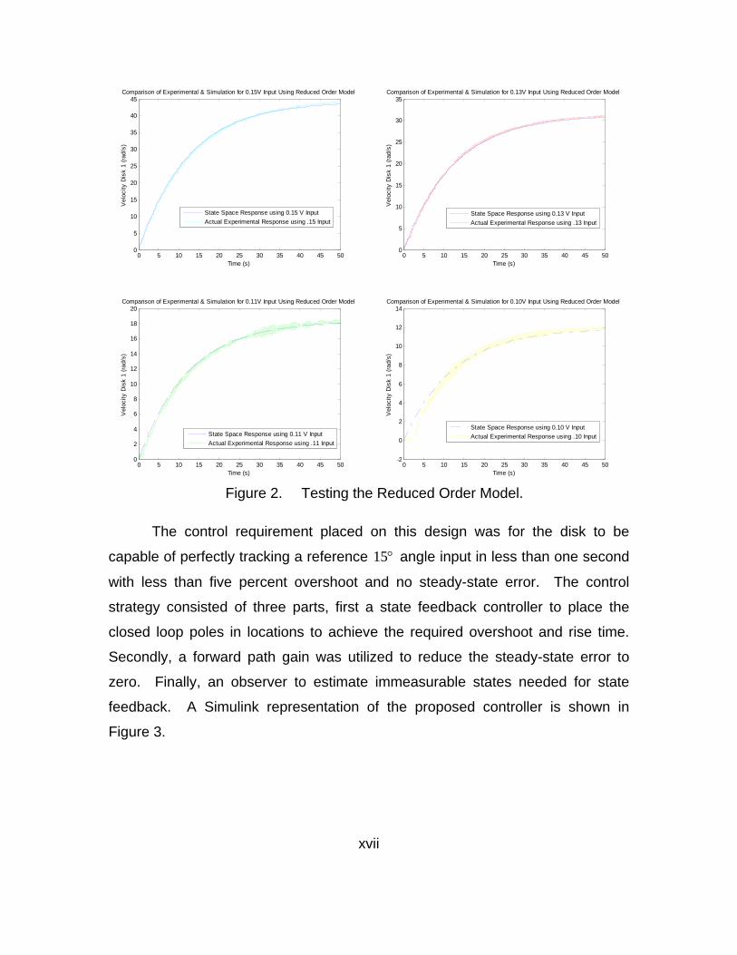
The reduced order model was then constructed in Simulink and the

accuracy of identified model parameters was verified by comparing the response

of the model using multiple step input voltages to the plant actual response. The

results for four input voltages are shown in Figure 2. Clearly, the model predicts

the actual behavior of the system for these inputs.

xvii

0 5 10 15 20 25 30 35 40 45 500

5

10

15

20

25

30

35

40

45

Time (s)

Vel

ocity

Dis

k 1

(rad

/s)

Comparison of Experimental & Simulation for 0.15V Input Using Reduced Order Model

State Space Response using 0.15 V Input

Actual Experimental Response using .15 Input

0 5 10 15 20 25 30 35 40 45 500

5

10

15

20

25

30

35

Time (s)

Vel

ocity

Dis

k 1

(rad

/s)




0 5 10 15 20 25 30 35 40 45 500

2

4

6

8

10

12

14

16

18

20

Time (s)

Vel

ocity

Dis

k 1

(rad

/s)




0 5 10 15 20 25 30 35 40 45 50-2

0

2

4

6

8

10

12

14

Time (s)

Vel

ocity

Dis

k 1

(rad

/s)




Figure 2. Testing the Reduced Order Model.

The control requirement placed on this design was for the disk to be

capable of perfectly tracking a reference 15° angle input in less than one second

with less than five percent overshoot and no steady-state error. The control

strategy consisted of three parts, first a state feedback controller to place the

closed loop poles in locations to achieve the required overshoot and rise time.

Secondly, a forward path gain was utilized to reduce the steady-state error to

zero. Finally, an observer to estimate immeasurable states needed for state

feedback. A Simulink representation of the proposed controller is shown in

Figure 3.

xviii

Figure 3. Final Control Design.

The control strategy was then tested using a 15° reference input to verify

that the performance objectives were met. This result is displayed in Figure 4.

0 0.5 1 1.5

-2

0

2

4

6

8

10

12

14

16Actual/Observed Angle of Disks if a 15 Degree Step Input

Am

plitu

de

Time (sec)

Actual Enc 1 position

Observer Enc 1 position

Figure 4. Closed Loop Plant Performance.

xix

Appendix A includes a series of six state-space laboratories applicable to

a course in state-space design that lead the student through the entire design

process from modeling through identification and finally control.

xx


xxi

ACKNOWLEDGMENTS

The author would like to give special thanks to Dr. Xiaoping Yun for his

insight, guidance, and eagerness to help with this thesis.

The author would also like to thank Dr. Alex Julian for his help as a reader,

and for his insights into this work.

The author would also like to acknowledge the contribution of James

Calusdian, who spent countless hours in the laboratory helping with equipment

and taking experiments.

Finally, the author would like to thank his wife, Isa, and his son, London,

for their constant support and patience during the work of this thesis.

xxii


1

I. INTRODUCTION

A. BACKGROUND

In the late 1960s, space exploration brought about a revolution in the

design methods used in control. Previous systems had been designed using so-

called classical methods, where individual subsystems were described first by

differential equations, followed by transfer functions that could be interconnected.

This interconnected block structure, as shown in Figure 5, each composed of a

single transfer function, simplified design of feedback controllers.

1

s+1

Subsystem 3

1

s+1

Subsystem 2

1

s+1

Subsystem 1 OutputInput

1

Gain1

1

Gain

Figure 5. Typical Classical Subsystem Control Structure.

The major advantage of these methods was how easily stability and

transient response information could be extracted from them. In short, the theory

and methods to vary pole location (root locus, lead-lag blocks) in order to shape

a systems response were well understood. The disadvantage of this approach

was that as systems grew in complexity (nonlinear, time-varying, high system

order and multiple input and outputs (MIMO)), the approaches either became too

difficult or lost their applicability [1].

Modern state-space design is a comprehensive term referring to modeling

and control of complex systems. The standard representation of a system is

shown below.

x Ax Bu y Cx Du= + = +& (1.1)

State-space design filled the void in that it compactly represents large

systems in matrix form, as well as being able to handle time-varying and non-

linear systems. Furthermore, the model’s B and C can be matrices allowing the

2

model to readily handle multiple inputs and outputs. Also, because the system is

represented compactly by matrices, it is easily manipulated by computers [2].

B. OBJECTIVE

The system explored in this thesis is a 4th order, single-input, multiple-

output torsion system from Educational Control Products, as shown in Figure 6.

Thus, the nature of the system lends itself to the state-space approach.

Figure 6. 4th Order Torsion Plant.

The methodology employed to model, identify, and control the fourth order

torsion plant set forth in this thesis is important to the Department of Defense

because it acts a template for which more complicated systems of much higher

order can be controlled. The techniques applied to control this system are easily

extrapolated to higher order systems.

One important goal of this thesis is that it is intended to introduce

introductory student to the entire state-space design process, from modeling to

identification and finally control. A review of current texts on control theory

[1][2][4][5][8] found that the model’s structure was assumed and the focus was on

the design a control strategy. In short, very little attention was paid to the

modeling and identification of the plant and a great deal of emphasis is placed its

control. The goal of this thesis is to bridge that gap by providing laboratories,

included in Appendix A, that show the introductory state-space control student a

robust method of modeling and identification that is applicable to a wide set of

problems as well as provide the fundamentals of control.

3

C. APPROACH

The modeling and identification approach taken in this thesis has several

components. First, a state-space model of the plant was developed by applying

first principles. Next, the unknown parameters in the model were found using

Matlabs parameter estimation toolbox from input / output data. This method could

also have been perform without making assumptions on the models underlying

structure, however, exploitation of the model physical structure proved to be

more insightful than using input/output data alone.

The control approach used is a pole placement strategy that utilizes state

feedback. This method allows the designer to choose pole placements that are

guaranteed to satisfy design criteria prior to simulation. This method was chosen

over root locus or frequency techniques that require an iterative process to

achieve a solution that meets the specifications.

D. ORGANIZATION

The thesis is organized in the following manner. In Chapter II, the state-

space model of the torsion plant will be derived from first principles. In Chapter

III, a method using parameter estimation will be used to identify individual entries

in the state-space model and conclusions will be made about its validity. Chapter

IV addresses system stability, steady-state-error, and whether the system is

controllable and observable. Finally, Chapter V introduces a pole placement

control strategy to move the system’s closed loop poles in such a manner that

specific performance criteria are met.

4


5

II. STATE-SPACE MODELING OF TORSION PLANT

In this chapter, the state-space model of a 4th order torsion plant will be

derived from first principles. To do this, a plant model that graphically depicts the

motion of the plant will be shown. The plant model will then be broken into two

components; an electrical model for the motor, and mechanical model for the

shaft and weights. These models will then be written as differential equations by

applying Newton’s 2nd Law and Kirchhoff’s Voltage Law. The higher order

differential equations can then be written compactly in state-space form by

introducing the state vector.

A. PLANT AND EQUIVALENT ELECTRICAL MODEL

The plant that will be modeled, and subsequently identified in this thesis,

is the rotational mechanical plant shown in Figure 7. This plant was chosen

because it complex enough to show that the modeling, identification and control

techniques employed are applicable to higher order systems yet it is still small

enough to be easily implemented. The plant consists of a shaft with two rotational

disks, each with their own two masses (500g each) attached at 7.5 cm from the

centerline of the shaft, is rotated by means of a DC Servo Motor. When a DC

voltage is applied, the shaft and disks begin to rotate. Higher input voltages

cause the shaft to spin faster and lower voltages slower. The increase in speed

with voltage is linear, once a sufficient voltage is input to overcome friction (the

region will later be referred to as the system’s dead-zone) and continues to be

linear for voltages in our region of interest. The angle of each disk is measured

by encoders.

6

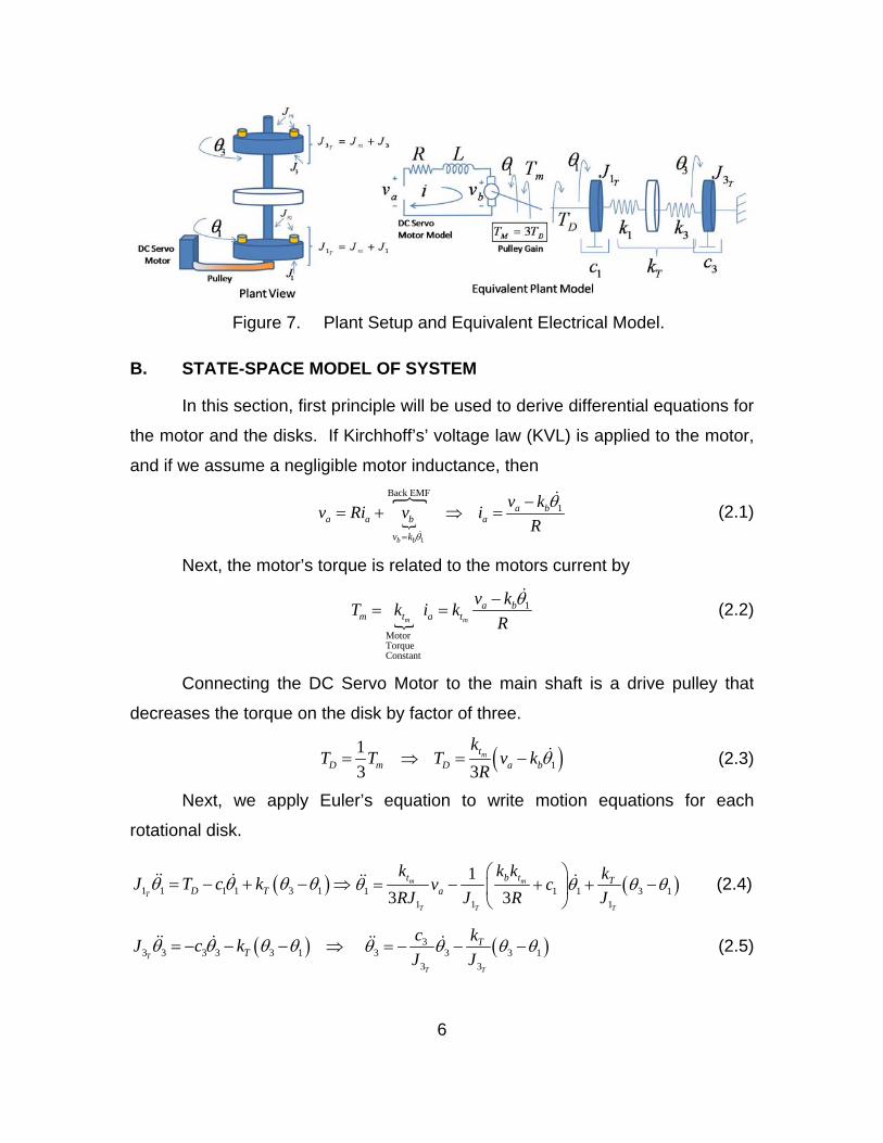
Figure 7. Plant Setup and Equivalent Electrical Model.

B. STATE-SPACE MODEL OF SYSTEM

In this section, first principle will be used to derive differential equations for

the motor and the disks. If Kirchhoff’s’ voltage law (KVL) is applied to the motor,

and if we assume a negligible motor inductance, then

{

}

1

Back EMF1

b b

a ba a b a

v k

v kv Ri v iR

θ

θ

=

−= + ⇒ =

&

& (2.1)

Next, the motor’s torque is related to the motors current by

{

1

MotorTorqueConstant

m m

a bm t a t

v kT k i kRθ−

= =&

(2.2)

Connecting the DC Servo Motor to the main shaft is a drive pulley that

decreases the torque on the disk by factor of three.

( )113 3

mtD m D a b

kT T T v k

Rθ= ⇒ = − & (2.3)

Next, we apply Euler’s equation to write motion equations for each

rotational disk.

( )1 1 1 1 3 1T D TJ T c kθ θ θ θ= − + − ⇒&& & ( )1 1 1 3 11 1 1

13 3

m m

T T T

t b t Ta

k k k kv cRJ J R J

θ θ θ θ⎛ ⎞

= − + + −⎜ ⎟⎝ ⎠

&& & (2.4)

( )3 3 3 3 3 1T TJ c kθ θ θ θ= − − − ⇒&& & ( )33 3 3 1

3 3T T

Tc kJ J

θ θ θ θ= − − −&& & (2.5)

7

If we define the state variable to be angular displacement and velocity of

each mass, 1 1 3 3

Tθ θ θ θ⎡ ⎤⎣ ⎦

& & , then a state-space representation can be written

11

1 1 1 111 1

33

333 3 3 3

0 1 0 0 01 0

3 30 0 0 1 0

0 0

m m

T T

T T

T T T

PLANTPLANT

b t tT T

a

T T

BA

k k kk J c k J

J R RJ v

k J k J c J

θθθθθθθθ

⎡ ⎤ ⎡ ⎤⎡ ⎤ ⎢ ⎥ ⎡ ⎤ ⎢ ⎥⎛ ⎞⎢ ⎥ ⎢ ⎥ ⎢ ⎥ ⎢ ⎥− − +⎜ ⎟⎢ ⎥ ⎢ ⎥ ⎢ ⎥ ⎢ ⎥= +⎝ ⎠⎢ ⎥ ⎢ ⎥ ⎢ ⎥ ⎢ ⎥⎢ ⎥ ⎢ ⎥ ⎢ ⎥ ⎢ ⎥⎢ ⎥ ⎣ ⎦⎣ ⎦ ⎢ ⎥ ⎢ ⎥− − ⎣ ⎦⎣ ⎦

&

&&&

&

&&&

14243144444444424444444443

(2.6)

The rotational plant is equipped with encoders that measure the rotation of

each of the masses in the system. From this data, the angular velocities of each

mass are also measured simply by differentiating the position data. Thus, access

to all system states is known. For future reference, when simulating the identified

model in Matlab, individual states can be obtained by defining 1 4...c c as either a 0

or 1, depending on the desired output.

{

11

12

33

34

0 0 00 0 0

00 0 00 0 0

PLANT

PLANT

D

C

cc

y uc

c

θθθθ

⎡ ⎤⎡ ⎤⎢ ⎥⎢ ⎥⎢ ⎥⎢ ⎥= +⎢ ⎥⎢ ⎥⎢ ⎥⎢ ⎥

⎣ ⎦ ⎣ ⎦

&

&1442443

(2.7)

C. SUMMARY

In this chapter, a state-space model of the 4th order torsion plant was

obtained from first principles. Next, a method of parameter estimation will be

presented to identify individual matrix entries.

8


9

III. MODEL IDENTIFICATION

In this chapter, a method of parameter estimation is utilized to identify the

entries in the state-space model. In short, Matlab’s parameter estimation function

found within the system identification toolbox will be employed to estimate the

state-space structure from experimental input and output data. As we will show,

this method is simple and efficient for identifying the linear region of our model. In

fact, in order to get a faithful system representation that works for all input and all

outputs, it will be necessary to identify the non-linear dead zone as well. Our final

model will then include two pieces, a dead zone and the linear portion. In the

chapter’s conclusion, a Simulink model will be produced and verification of the

state-space model will be performed.

A. MODELING THE SYSTEM’S DEAD-ZONE

A dead-zone refers to the range of voltages that, if applied to the system,

do not result in moving the shaft because they are not great enough to overcome

the system’s friction. This dead-zone is the primary culprit for the nonlinear

behavior of the system and, if it can be identified first, other techniques can be

used to identify the remaining linear portion.

To identify the dead zone, we need to find the first voltage that causes the

shaft to move. To do this, we will start by applying a step voltage of 0.15 V and

measure the corresponding steady-state speed of the shaft. Next, we will

decrease the voltage to 0.13V, then 0.11V, and finally 0.10V, again measuring

the steady-state shaft speed each time. The dead-zone voltage can then be

found through extrapolation, as shown in Figure 8.

10

0 0.02 0.04 0.06 0.08 0.1 0.12 0.14 0.160

5

10

15

20

25

30

35

40

45

50Final Velocity vs Applied Voltage

Applied Voltage (V)

Fin

al V

eloc

ity (

Rad

/sec

)

y = 648*x - 52.9

Dead Zone Voltage

Figure 8. Extrapolation to Find Dead-zone.

As shown in the Figure 8, the system has a dead-zone of 0.0816 V.

Hence, applied voltages below this value do not result in an output, and voltages

above this are assumed to increase the velocity in a linear fashion.

The system’s dead zone can then be modeled in Simulink using the

following structure block in Figure 9.

Figure 9. Implementation of the Non-linear Dead-zone Block in Simulink.

In the next section, a method is shown to estimate the remaining linear

region of the torsion plant.

B. SYSTEM IDENTIFICATION VIA PARAMETER ESTIMATION

This section is meant to provide an introduction to the system identification

toolbox in Matlab. The information contained here is summarized from the

toolbox help files. In the following summary, the tools discussed are used to

identify the complex 4th order system presented in Chapter II. Simulink’s system

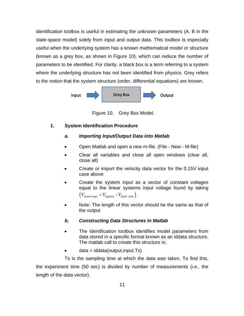
11

identification toolbox is useful in estimating the unknown parameters (A, B in the

state-space model) solely from input and output data. This toolbox is especially

useful when the underlying system has a known mathematical model or structure

(known as a grey box, as shown in Figure 10), which can reduce the number of

parameters to be identified. For clarity, a black box is a term referring to a system

where the underlying structure has not been identified from physics. Grey refers

to the notion that the system structure (order, differential equations) are known.

Figure 10. Grey Box Model.

1. System Identification Procedure

a. Importing Input/Output Data into Matlab

• Open Matlab and open a new m-file. (File - New - M-file)

• Clear all variables and close all open windows (clear all, close all)

• Create or import the velocity data vector for the 0.15V input case above

• Create the system input as a vector of constant voltages equal to the linear systems input voltage found by taking ( )system input applied dead zoneV V V −= − .

• Note: The length of this vector should be the same as that of the output

b. Constructing Data Structures in Matlab

• The identification toolbox identifies model parameters from data stored in a specific format known as an iddata structure. The matlab call to create this structure is:

• data = iddata(output,input,Ts) Ts is the sampling time at which the data was taken. To find this,

the experiment time (50 sec) is divided by number of measurements (i.e., the

length of the data vector).

12

c. Constructing a Continuous-time State-space Model Object

A state-space model object is similar to a storage unit that contains

all the information about a state-space model. It not only contains the state-

space model, but provides the user with the ability to specify parameters that are

going to be estimated from given data. Creating a state-space model is done

using:

Model_object=idss(A,B,C,D,K,x0,'Ts',0);1

Setting up the model object is done in three steps, first we define a

nominal parameter model inserting in only the known entries.2 Second, we create

the object, and third, we specify which entries in the model we desire Matlab to

do parametric analysis on. These steps are shown below.

• Defining a nominal model3: insert only the known entries. A = [0 1 0 0 ; 0 0 0 0;0 0 0 1;0 0 0 0]; B = [0 0 0 0]'; C = [0,1,0,0]; D = 0; K = zeros(4,1); x0 = [0;0;0;0];

• Create the model object using Model_object=idss(A,B,C,D,K,x0,'Ts',0);

• Specifying parameters to be estimated

To display the information contained in the model object first run

the m-file and at the Matlab prompt type get(m).4 This shows the properties of

the stored object. Notice that in the middle of the object there exists other data

1 Continuous and Discrete state-space models can be stored as objects. To distinguish the

two, the sampling time is set to zero in the continuous model. 2 The continuous time state-space representation in Matlab includes a noise term which

should be set to zero. x Ax Bu Kw y Cx Du w= + + = + +& 3 Unknown values in the model (i.e., a, b) should be initialized with best guesses. If unknown,

zero should be used. 4 Individual entries of the structure can be seen by entering m.(desired entry) at the Matlab

prompt.

13

areas that can be used in parameterization. It is those structures that we will

used to tell Matlab which entries in our model are parameters to be identified. SSParameterization: 'Structured' As: [4x4 double] Bs: [4x1 double] Cs: [0 1 0 0] Ds: 0 Ks: [4x1 double] X0s: [4x1 double]

To specify which parameters are to be estimated, Matlab requires

the NaN symbol be used as shown below: m.As = [0 1 0 0;0,NaN NaN NaN 0; 0 0 0 1; NaN 0 NaN NaN]; m.Bs = [0 NaN 0 0]'; m.Cs = [0 1 0 0]; m.Ds = 0; m.Ks = m.k; m.x0s = [0;0;0;0];

The NaN does not refer to not a number in the traditional

mathematical sense, but rather is used to designate which parameters the user

wants the parameter estimation performed upon.

d. Perform Parameter Estimation

Matlab has a function, PEM, for parameter estimation upon state-

space objects, which requires both data (output data structure) and the state-

space model object (m). It can be implemented as follows:

m =pem(data,m)

e. Extracting the State-space Model

• The state-space model can be extracted from the m object structure by

• [A,B,C,D]=ssdata(m)

2. Results

The parameter identification procedure outlined above gives the following

state-space model

14

[ ]5

0 1 0 0 01.605 10 .0756 0 0 49.9655

0 1 0 00 0 0 1 00 0 0 0 0

xA B C

−

⎡ ⎤ ⎡ ⎤⎢ ⎥ ⎢ ⎥− −⎢ ⎥ ⎢ ⎥= = =⎢ ⎥ ⎢ ⎥⎢ ⎥ ⎢ ⎥⎣ ⎦ ⎣ ⎦

(3.1)

Interestingly, the A matrix above is rank deficient with the 3rd and 4th

states disconnected from the first two. Converting this state-space structure into

a transfer function and finding its minimal realization indicates that the system

behaves as a second order system.

( )2 5

49.97( ) .07558 1.605 10s s

V s s s xθ

−=+ +

(3.2)

Why? One possibility is that the shaft is so inflexible that it should not be

modeled as a spring. If this is true, the shaft simply couples the two disks,

forming one larger mass (a second order system). To confirm this, an input

voltage was given and the angles of both disks were recorded in time, as shown

in Figure 11. Clearly, the angles move together and are only separated by less

than 0.05 degrees for a 0.13 V input. Again, this is due to the shaft not deflecting.

15

0 5 10 15 20 25 30 35 40 45 500

0.5

1

1.5

2

2.5

3

3.5x 10

6 Comparison of Disk 1 Angle and Disk 2 Angle

time (s)

Ang

le (

coun

ts)

Disk 1 Angle

Disk 3 Angle

34.3385 34.339 34.3395 34.34 34.3405 34.341 34.3415 34.342 34.3425

1.8238

1.8239

1.8239

1.824

1.824

x 106 Comparison of Disk 1 Angle and Disk 2 Angle

time (s)

Ang

le (

coun

ts)

Disk 1 Angle

Disk 3 Angle

Plot magnified to show only a slight difference in angle between disk 1 and 3

Figure 11. Disk 1, 3 Angle using a 0.13V Input.

We conclude the following:

Modeling a shaft as a spring has only limited utility unless

• The shaft is sufficiently flexible so that normal input voltages results in appreciable changes in angles between both disks.

• The goal is to model and control the system in a small angle sense. (Disk one and two are only different over a small range.

• The voltage input is large enough that a large deflection in the shaft occurs.

• Sinusoidal voltages are input. For the system presented above, none of these criteria were met. Thus, it

is proposed that a reduced order model would be simpler while maintaining the

main characteristics of the problem.

16

C. REDUCED ORDER MODEL

Consider the shaft inflexible and group the masses, as shown in Figure

12.

Figure 12. Reduced Order Plant Model.

As before, applying KVL to the motor and assume a negligible motor

inductance,

{

}

1

Back EMF1

b b

a ba a b a

v k

v kv Ri v iR

θ

θ

=

−= + ⇒ =

&

& (3.3)

Then the motor’s torque is related to the motors current by

{

1

MotorTorqueConstant

m m

a bm t a t

v kT k i kRθ−

= =&

(3.4)

Connecting the DC Servo Motor and the main shaft is a drive pulley that

decreases the torque on the disk by factor of three.

( )113 3

mtD m D a b

kT T T v k

Rθ= ⇒ = − & (3.5)

Next, we sum the moments about the rotational axis and simplify

{

13 3

m m

T

T

t b tD a a

T

b a

k k kJ T c v c a bv

RJ J Rθ θ θ θ θ

⎛ ⎞= − ⇒ = − + = − +⎜ ⎟

⎝ ⎠&& & && & &

1442443

(3.6)

1 ax ax bv= − +& (3.7)

where we have let 11 1

1 and 3 3

m m

T T

b t tk k ka c b

J R RJ⎛ ⎞

= + =⎜ ⎟⎝ ⎠

for simplicity.

17

Writing this in state-space form results in

0 1 00 av

a bθθθθ

⎡ ⎤ ⎡ ⎤ ⎡ ⎤ ⎡ ⎤= +⎢ ⎥ ⎢ ⎥ ⎢ ⎥ ⎢ ⎥−⎣ ⎦ ⎣ ⎦ ⎣ ⎦⎣ ⎦

&

&&& (3.8)

D. IDENTIFICATION OF REDUCED ORDER MODEL

The method employed here to identify the parameters a,b of the state-

space model was adapted from laboratories developed by Yun [3]. It works well

for 2nd order systems. First, if we take the Laplace transform of (3.7) above and

recognizing that the initial angular velocity is zero (i.e., ( )0 0x = ), then

( ) ( )0X s X− ( ) ( ) ( )

( )( )( )1

aa

a

b V sbV s aaX s bV s X sss aa

= − + ⇒ = =+ ⎛ ⎞+⎜ ⎟

⎝ ⎠

(3.9)

If we let mbKa

= and 1aτ

= where τ is the systems time constant

( ) ( )( )1

m aK V sX ssτ

=+

(3.10)

Since the voltage is a step input ( ) 0aa

vV s ts

= ≥ , then in the time domain,

( ) ( )}

( )

( ) 11 a

InvLaplace

tm a m am

K v K vX s x t K v es s

τ

τ−= − = ⇒ = −

+ (3.11)

By making these definitions our goal is to first find mK by letting t →∞ for a

given input voltage. The input voltage in this case would be a applied dead zonev v v −= − ,

which more accurately represents the voltage applied to the system after the

dead-zone.

18

The time constant,τ , represents the time it takes the system's step

response to reach approximately 63% of its final (asymptotic) value as shown in

Figure 13. With ,mK τ known a, b can also be found from their definitions, which

have been restated below for clarity,

1,mbK aa τ

= = (3.12)

0 5 10 15 20 25 30 35 40 45 500

5

10

15

20

25

30

35

Time (seconds)

Vel

ocity

(ra

d/se

c)

Experimental System Response to a Step Input = 0.13V

63% of Final Value

Time Constant = 13.08 sec

Final Velocity = 31 rad/sec

Figure 13. Experimental Velocity Response to a 0.13 V Input.

From this data, , , ,mK a bτ can be found

646.89 .08113.08 52.41

mK abτ

= == =

(3.13)

The reduced order state-space model is therefore,

0 1 00 .081 52.41 av

θθθθ

⎡ ⎤ ⎡ ⎤ ⎡ ⎤ ⎡ ⎤= +⎢ ⎥ ⎢ ⎥ ⎢ ⎥ ⎢ ⎥−⎣ ⎦ ⎣ ⎦ ⎣ ⎦⎣ ⎦

&

&&& (3.14)

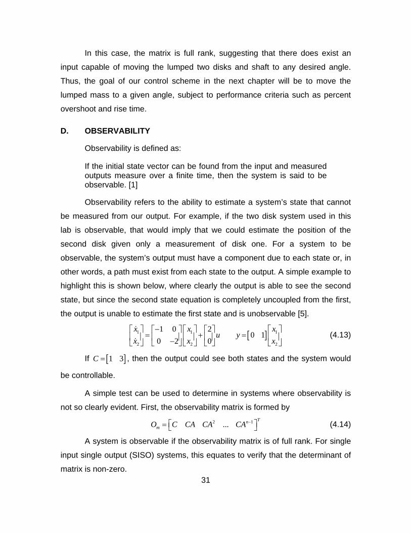
As confirmation that this reduced order model well-represents the actual

experimental out of our system, a state-space model as shown in Figure 14 was

constructed and the response plotted against the experimental data in Figure 15.

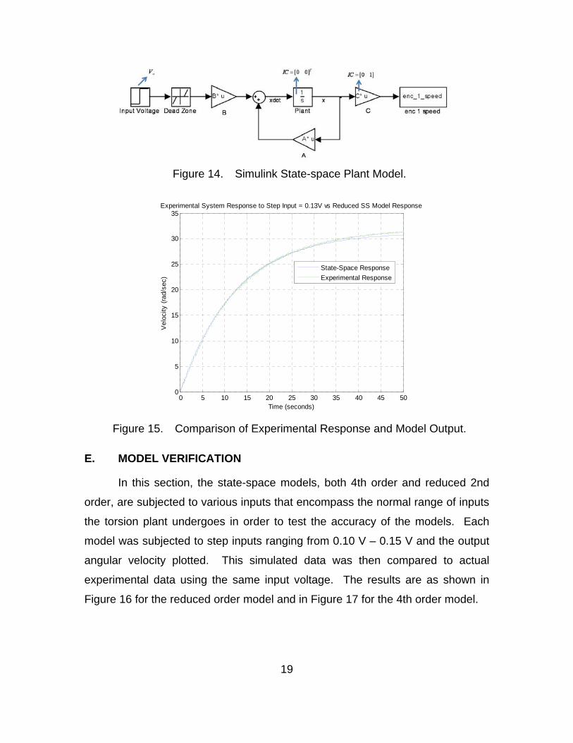
19

Figure 14. Simulink State-space Plant Model.

0 5 10 15 20 25 30 35 40 45 500

5

10

15

20

25

30

35

Time (seconds)

Vel

ocity

(ra

d/se

c)

Experimental System Response to Step Input = 0.13V vs Reduced SS Model Response

State-Space Response

Experimental Response

Figure 15. Comparison of Experimental Response and Model Output.

E. MODEL VERIFICATION

In this section, the state-space models, both 4th order and reduced 2nd

order, are subjected to various inputs that encompass the normal range of inputs

the torsion plant undergoes in order to test the accuracy of the models. Each

model was subjected to step inputs ranging from 0.10 V – 0.15 V and the output

angular velocity plotted. This simulated data was then compared to actual

experimental data using the same input voltage. The results are as shown in

Figure 16 for the reduced order model and in Figure 17 for the 4th order model.

20

0 5 10 15 20 25 30 35 40 45 500

5

10

15

20

25

30

35

40

45

Time (s)

Vel

ocity

Dis

k 1

(rad

/s)




0 5 10 15 20 25 30 35 40 45 500

5

10

15

20

25

30

35

Time (s)

Vel

ocity

Dis

k 1

(rad

/s)




0 5 10 15 20 25 30 35 40 45 500

2

4

6

8

10

12

14

16

18

20

Time (s)

Vel

ocity

Dis

k 1

(rad

/s)




0 5 10 15 20 25 30 35 40 45 50-2

0

2

4

6

8

10

12

14

Time (s)

Vel

ocity

Dis

k 1

(rad

/s)




Figure 16. Verification of Reduced Order Model.

21

0 5 10 15 20 25 30 35 40 45 500

5

10

15

20

25

30

35

40

45

Time (s)

Vel

ocity

Dis

k 1

(rad

/s)

Comparison of Experimental & Simulation for 0.15V Input Using 4th Order Model



0 5 10 15 20 25 30 35 40 45 500

5

10

15

20

25

30

35

Time (s)

Vel

ocity

Dis

k 1

(rad

/s)




0 5 10 15 20 25 30 35 40 45 500

2

4

6

8

10

12

14

16

18

20

Time (s)

Vel

ocity

Dis

k 1

(rad

/s)




0 5 10 15 20 25 30 35 40 45 50-2

0

2

4

6

8

10

12

14

Time (s)

Vel

ocity

Dis

k 1

(rad

/s)




Figure 17. Verification of 4th Order Model.

The reduced order model is very accurate for all constant voltage inputs.

Only one significant deviation is seen at the start of the experiment for low

voltages (see 0.10V input above). The most likely cause is that 0.10 V is

approaching the dead-zone voltage (0.0816 V) where the effects of friction begin

to dominate and thus a linear model is not accurate. Note, however, that this is a

flaw with both the 4th and 2nd order models as both are linear models.

Comparison of the performance of both models validates the claim that

indeed this system behaves as a second order system. This lends credence to

notion that care must be used when modeling shafts as springs. Here, for

example, the shaft was so inflexible that it coupled the two disks making them act

as one, effectively reducing the systems order to two.

22

F. SUMMARY

In this chapter, the 4th order state-space model derived in chapter two

was identified. The model consisted of two parts, a nonlinear dead-zone and a

linear region. Interestingly, the results suggested that the 4th order model could

be well represented by a reduced second order model. The reduction in order

was unexpected; however it could be explained using common sense. The

reduction arose because the shaft was modeled as a spring, however since the

shaft was very rigid, it behaved as an inflexibly structure tying the masses

together and thus reducing the order to two.

In the introduction an overall design path for the torsion plant was laid out.

First the system was to be modeled, and then identified. Finally a pole placement

control strategy would be employed in which either disk could be moved to a

given desired reference angle with a specified percent overshoot and in a given

time. However, since this system is uncontrollable (owing to the fact that the

controllability matrix is rank deficient due of the inflexible shaft), it would be

impossible to command disk one to 15 degrees and simultaneously command

the second disk to 25 degrees.

In light of this finding, the goal of this design should be more realistic.

Now, the goal is to move both disks to a given angle in a specified time with a

specified percent overshoot and with no steady-state error.

23

IV. STABILITY, STEADY-STATE ERROR, CONTROLLABILITY AND OBSERVABILITY

In this chapter, four fundamental system properties will be studied in detail

from a state-space point of view as each will have an impact on the control

strategy used on the torsion plant. The first property, stability, is key to

understanding the behavior of the system. Secondly, steady-state error is a key

analytic tool used to determine how well the system tracks the desired trajectory.

Finally, the concepts of controllability and observability will be discussed in order

to determine whether the torsion plant is well suited to a pole placement control

strategy utilizing an observer.

A. STABILITY

Two common definitions of stability are

• If a system is subjected to a bounded input and the response is bounded in magnitude, then the system is stable [4].

• A system is unstable if the natural response approaches infinity as time goes to infinity [1].

System pole locations give insight into the natural response of a system

and, thus, its stability. For example, a left-hand plane pole (examples 2s = − or

3 2s j= − ± ), as shown in Figure 18, yields either a damped sinusoid or a

exponential decay as their time response, whereas poles on the jw axis or in the

right half plane (example 2s = or 2 2s j= ± ), as shown in Figure 19, lead to

unstable or exponentially increasing responses.

• Conclusion: Poles located in the LHP result in stable systems.

24

-4 -2 0 2-0.2

-0.1

0

0.1

0.2Stable Poles

Real Axis

Imag

inar

y A

xis

-20 -10 0 10-50

0

50Stable Poles

Real Axis

Imag

inar

y A

xis

0 0.5 1 1.5 20

0.5

1Impulse Response

Time (sec)

Am

plitu

de

0 0.1 0.2 0.3 0.4-0.01

0

0.01

0.02Impulse Response

Time (sec)A

mpl

itude

LHP LHP

Figure 18. Left Half Plane Poles Time Domain Response.

-0.5 0 0.5 1 1.5-0.2

-0.1

0

0.1

0.2Unstable Poles

Real Axis

Imag

inar

y A

xis

-1 0 1 2 3-4

-2

0

2

4Unstable Poles

Real Axis

Imag

inar

y A

xis

0 5 10 150

1

2

3

4x 10

6 Impulse Response

Time (sec)

Am

plitu

de

0 2 4 6 8-4

-2

0

2x 10

6 Impulse Response

Time (sec)

Am

plitu

de

RHP RHP

Figure 19. Right Half Plane Time Domain Response.

25

1. Calculating Poles of a State-space System

For the state-space system,

x Ax Buy Cx= +=

& (4.1)

the transfer function ( )( )

Y sU s

is formed by taking the Laplace Transform ignoring

initial conditions and solving for X(s),

( ) 1( ) (0) ( ) ( ) ( ) ( )sX s X AX s BU s X s sI A BU s−− = + ⇒ = − (4.2)

This relation is then used in the equation for Y(s) and simplified

( ) 1( ) ( ) ( )Y s CX s C sI A BU s−= = − (4.3)

( ) 1( ) * ( )*( ) det( )

Y s C adj sI A BC sI A BU s sI A

− −= − =

− (4.4)

where we have employed the mathematical notion that

( ) 1 ( )det( )adj sI AsI A

sI A− −

− =−

(4.5)

Clearly, the system’s poles are the solution to det( )sI A− or, in other words,

the eigenvalues of the A matrix [1].

• For a state-space system, [A, B, C, D], the eigenvalues of [A] represent the poles of the system.

2. Stability of Reduced Order Model

0 1 00 .081 52.41 av

θθθθ

⎡ ⎤ ⎡ ⎤ ⎡ ⎤ ⎡ ⎤= +⎢ ⎥ ⎢ ⎥ ⎢ ⎥ ⎢ ⎥−⎣ ⎦ ⎣ ⎦ ⎣ ⎦⎣ ⎦

&

&&& (4.6)

The reduced order model given above has two poles, one at -0.081 and

the other at the origin. By definition, this is a marginally stable system. The

significance of the term “marginally stable” refers to the notion that the system

has one pure integrator (between the angle and angular velocity). The

consequence of being marginally stable is that constant step voltage inputs are

26

integrated and result in unbounded behavior. In our problem, when a constant

DC input is applied to the servo motor, the shaft rotates constantly and the shaft

angle gets larger and larger.

B. STEADY-STATE ERROR

Steady-state error is an important performance tool for determining how

accurately a control strategy is performing. For example, in the case of the

torsion plant, if a 15 degree disk rotation is commanded and the disks rotates 20

degrees or more, this would be an important performance criteria to be

concerned with. In this section we will introduce the theory behind calculating the

steady-state error and apply it to the open loop system. Later, in Chapter V, it will

be applied to the closed loop system. The following derivation is taken from [1].

For the state-space model shown in Figure 20,

x Ax Bry Cx= +=

& (4.7)

Figure 20. Standard State-space Model (left); Definition of Error (right).

The error ( ) ( ) ( )E s R s Y s= − can be combined with ( ) 1( )( )

Y s C sI A BR s

−= −

( ) 1( ) ( ) 1E s R s C sI A B−⎡ ⎤= − −⎣ ⎦ (4.8)

To find the steady-state error, the final value theorem is used,

( ) 1

0lim ( ) 1s

error sR s C sI A B−∞ →

⎡ ⎤= − −⎣ ⎦ (4.9)

( )1where ( ) unit stepR ss

=

27

The goal of this section is to demonstrate how the steady-state error could

be calculated for the reduced order plant. To do this, we assume that a

reference 1 volt step input is applied to the plant. Also, we will assume that the

plant’s output is shaft velocity, as shown in Figure 21.

Figure 21. Velocity Steady-state Error.

The conversion was found through experimentation. It is the slope (see

Figure 8) of the velocity vs. voltage graph in the dead-zone experiment. The

conversion is necessary to ensure the reference and the output have equivalent

units.

The error can now be written as ( )( ) ( )648Y sE s R s= − . Also, the steady-state

error equation can be modified as

( ) 1

0lim ( ) 1

648s

C sI A Berror sR s

−

∞ →

⎡ ⎤−= −⎢ ⎥

⎢ ⎥⎣ ⎦

[ ]

( )

1

0 0

1 00 1

0 0.081 52.411 52410 647lim 1 lim 1 1 0648 648 1000 81 648s s

ss

error ss s

θ

−

∞ → →

⎡ ⎤−⎛ ⎞ ⎡ ⎤⎢ ⎥⎜ ⎟ ⎢ ⎥ ⎡ ⎤+⎢ ⎥⎝ ⎠ ⎣ ⎦= − = − = − ≈⎢ ⎥⎢ ⎥ +⎣ ⎦⎢ ⎥⎢ ⎥⎣ ⎦

&

Thus, there is zero velocity error to a step voltage input. To verify this result, a

Simulink Model of the reduced plant was given a step input; the results are

shown in Figure 22.

28

0 10 20 30 40 50 60 70 80 90 1000

0.1

0.2

0.3

0.4

0.5

0.6

0.7

0.8

0.9

1Response of Reduced Order Plant to Step Voltage Input

Time (sec) (sec)

Vel

ocity

(ra

d/se

c)

Figure 22. Velocity Response to a 1 Volt Step Input.

From the preceding analysis, the system appears to behave as a type one

system with zero steady-state error to a step voltage input. The concept of

steady-state error will play a role later, when our goal will be to drive the shaft

angle to 15 degrees with no steady-state error. In that analysis, the simulation

approach will be used over the more difficult application of the formula.

29

C. CONTROLLABILITY

Controllability is defined as follows:

If an input to a system can be found that takes every state variable from a desired initial state to a desired final state the system is said to be controllable, otherwise it is uncontrollable. [1]

The first step in the full state variable design process is to determine

whether or not the control input, u, is capable of moving each state to any

desired location. Or, in other words, can the control input affect each state. If the

input does not affect all the states, we say that the system is uncontrollable and it

is impossible to place the closed poles anywhere we desire. Note, however, that

a system that is uncontrollable is not necessarily unstable. A problem does arise

if the uncontrollable state is unstable, as the controller will not be able to stabilize

it. A simple example of this idea is the state-space model shown below, where

the input directly affects the first state equation; unfortunately, that equation is

completely uncoupled from the second state. Thus, the input cannot move the

second state and the system is uncontrollable [5].

1 1

2 2

1 0 20 2 0

x xu

x x−⎡ ⎤ ⎡ ⎤⎡ ⎤ ⎡ ⎤

= +⎢ ⎥ ⎢ ⎥⎢ ⎥ ⎢ ⎥−⎣ ⎦ ⎣ ⎦⎣ ⎦ ⎣ ⎦

&

& (4.10)

If the system above instead had [ ]2 1 TB = , the system would be

controllable.

Unlike the simple example above, there is usually difficulty in visually

determining whether a system is controllable, due to the size and complexity of

the state-space model. In such cases, a simple test can be used to determine

whether a system is controllable. The derivation can be found in [5]. First, the

controllability matrix is formed by 2 1... n

mC B AB A B A B−⎡ ⎤= ⎣ ⎦

30

A system is controllable if the controllability matrix is of full rank. For

single input single output (SISO) systems this equates to verifying that the

determinant of the controllability matrix is non-zero.

• In Matlab, the function CTRB finds the systems controllability matrix and the RANK can check the rank [6].

1. Controllability of the 4th Order Model

Matlab was used to calculate the controllability of the 4th order model. The

result is given below.

0 49.96 3.77 0.2849.96 3.77 0.28 .02

20 0 0 00 0 0 0

mC Rank

−⎡ ⎤⎢ ⎥− −⎢ ⎥= =⎢ ⎥⎢ ⎥⎣ ⎦

(4.11)

The reason the 4th order model’s controllability matrix is rank deficient is

that the shaft that connects the two masses is not flexible enough to exhibit a

spring-like behavior. In reality, the difference in angle between the disks is

extremely small. Thus, from the perspective of the input motor, the two disks

separated by a shaft appear to be a single disk moving at one speed. This result

supports the notion that the modeling of a rigid shaft as a spring is not

appropriate in this case. Clearly, for the actual system, it is impossible to find an

input that moves one disk to 15 degrees while simultaneously moving the second

disk to 30 degrees. Hence, the actual system is not controllable and this is

reflected in the work above.

2. Controllability of the Reduced Order Model

If we turn our attention to the reduced order model found by treating the

shaft and disks as a single mass spinning together, the controllability matrix is

given by

0 52.41

252.41 4.25mC Rank⎡ ⎤

= =⎢ ⎥−⎣ ⎦ (4.12)

31

In this case, the matrix is full rank, suggesting that there does exist an

input capable of moving the lumped two disks and shaft to any desired angle.

Thus, the goal of our control scheme in the next chapter will be to move the

lumped mass to a given angle, subject to performance criteria such as percent

overshoot and rise time.

D. OBSERVABILITY

Observability is defined as:

If the initial state vector can be found from the input and measured outputs measure over a finite time, then the system is said to be observable. [1]

Observability refers to the ability to estimate a system’s state that cannot

be measured from our output. For example, if the two disk system used in this

lab is observable, that would imply that we could estimate the position of the

second disk given only a measurement of disk one. For a system to be

observable, the system’s output must have a component due to each state or, in

other words, a path must exist from each state to the output. A simple example to

highlight this is shown below, where clearly the output is able to see the second

state, but since the second state equation is completely uncoupled from the first,

the output is unable to estimate the first state and is unobservable [5].

[ ]1 1 1

2 2 2

1 0 20 1

0 2 0x x x

u yx x x

−⎡ ⎤ ⎡ ⎤ ⎡ ⎤⎡ ⎤ ⎡ ⎤= + =⎢ ⎥ ⎢ ⎥ ⎢ ⎥⎢ ⎥ ⎢ ⎥−⎣ ⎦ ⎣ ⎦⎣ ⎦ ⎣ ⎦ ⎣ ⎦

&

& (4.13)

If [ ]1 3C = , then the output could see both states and the system would

be controllable.

A simple test can be used to determine in systems where observability is

not so clearly evident. First, the observability matrix is formed by

2 1...Tn

mO C CA CA CA −⎡ ⎤= ⎣ ⎦ (4.14)

A system is observable if the observability matrix is of full rank. For single

input single output (SISO) systems, this equates to verify that the determinant of

matrix is non-zero.

32

• In Matlab, the function OBSV finds the system’s observability matrix [7].

1. Observability of the 4th Order Model

The observability matrix for the 4th order model is given by

0 49.96 3.77 .284749.96 3.77 .2847 .0215

20 0 0 00 0 0 0

mO Rank

−⎡ ⎤⎢ ⎥− −⎢ ⎥= =⎢ ⎥⎢ ⎥⎣ ⎦

(4.15)

Again, the 4th order system is not observable, primarily due to the same

reason it was not controllable, i.e., the shaft is inflexible. It is meaningless to

estimate the position of one disk from the position of the other when, in essence,

they are all one lumped mass.

2. Observability of the Reduced Order Model

1 00 1

20 10 0.081

mO Rank

⎡ ⎤⎢ ⎥⎢ ⎥= =⎢ ⎥⎢ ⎥−⎣ ⎦

(4.16)

For the reduced order model, being observable has a somewhat more

useful meaning than before; it suggests that it is possible to estimate the angular

velocity simply from measurements of the position (without the need for

differentiation). This idea is exploited in the following chapter on control.

E. SUMMARY

In this chapter, the torsion system was shown to be marginally stable.

Steady-state error was introduced and applied to the open loop reduced order

system. The system behaved as a type one system, with zero steady-state error

to a step when velocity was the output.

It was shown that the 4th order system was not controllable; thus, we will

not concern ourselves with attempting to move the disks to two separate

positions. Rather, the goal is to control both disks together. Hence, the following

33

chapter will utilize the reduced order model exclusively. The analysis on

observability suggested that an observer design is possible, that estimates the

angular velocity of the lumped disks from the angle data alone.

In the next chapter, a pole placement control strategy will be employed to

move the system’s poles in such a manner that, when a one degree rotation of

disk one is commanded, the system will rotate one degree with less than five

percent overshoot and have a rise time less than one second.

34


35

V. POLE PLACEMENT DESIGN

The main thrust of this chapter will be to introduce a pole placement

design strategy, known as state feedback, that will move the closed loop poles so

as to achieve less than five percent overshoot and a rise time less than one

second when a reference position input of 15 degrees is commanded. In the first

part of this chapter, full state feedback is described, and then implemented.

Next, we assume access to all the system’s states is not available (specifically,

we assume the angular velocity is not measured), and a state observer is

designed to estimate the state.

A. FULL STATE VARIABLE FEEDBACK

As the name implies, full state variable feedback is a pole placement

design technique by which all desired poles are selected at the start of the design

process. A graphical representation of the closed loop plant and control is shown

in Figure 23. To show that this approach has the ability to place the poles in any

desired location, first assume the reference is zero, the input is simply u Kx= − ,

and the state equations become

( )x Ax Bu x A BK x= + ⇒ = −& & (5.1)

which has a solution of ( ) ( ) ( )0 A BK tx t x e− −= [5]. Thus, proper selection of gains, K,

can change the system’s response as desired. As one can readily see, each

state is multiplied by a predetermined constant and before being returned. Thus,

full state feedback simply means that each state is fed back. Consequently, this

scheme requires all states of the torsion plant, both the angle and angular

velocity of each disk, to be measured and fed back. If all states can’t be

measured directly, or if cost prohibits their measurement, an observer can be

designed to first estimate the plant’s states, then state estimates are fed back.

36

One might venture to ask how state feedback is better than other pole

placement strategies. This technique is more robust than other pole placement

schemes, such as root locus or looking at the transfer function’s frequency

response, in that these methods design a controller based on the dominate 2nd

order poles and hope that additional poles do not significantly alter response.

State feedback is applicable to systems with many states, and has the additional

advantage that all closed loop poles are chosen at the onset of the design

process, as we shall see shortly.

Figure 23. Full State Variable Feedback.

1. State Feedback Design

The goal of this design is for the torsion plant, modeled as a reduced

second order system, to be capable of moving to within 98% of any desired

reference angle in less than one second, and have less than 5% overshoot in the

process. These criteria were selected because they are commonly used in

control literature. They are summarized below:

Given: 1sT = second; % % 5%Overshoot OS= =

Using the performance criteria given above, our first task is to find a

transfer function pair whose dominant poles meet these requirements. These

poles represent where we would like our open loop poles to migrate so that once

the control is implemented we have acceptable performance. The method is

outlined below,

37

• Calculate the system’s damping ratio

( )( )

( )( )2 2 2 2

ln % /100 ln 5 /100.689

ln % /100 ln 5 /100

OS

OSξ

π π

− −= = =

+ + (5.2)

• Calculate the system’s natural frequency

( )( )

4 4 4 5.77.6925 1s n

n s

TT

ωξω ξ

= ⇒ = = = (5.3)

• Use the above to find our desired 2nd order transfer function whose poles

meet the design objectives. Find the poles of this transfer function, which represent the dominant poles.

2

2 2 2

33.29( )2 7.95 33.29

ndesired

n n

G ss s s s

ωξω ω

= =+ + + +

(5.4)

• The roots of the desired transfer function are the system’s poles.

1,2 3.975 4.182p j= − ± (5.5)

Again, it is emphasized that the desired transfer function has pole

locations that the closed loop system must have in order to attain the

performance criteria (percent overshoot and rise time) outlined above.

2. Calculating Feedback Gains

In this section, a method is described for finding the state feedback gains,

[ ]1 2K k k= , in order to place the closed loop poles as described in the previous

section.

The closed loop system of the state-space system x Ax Bu= +& where

fu K r Kx= − is given by:

( ) f CL CLx A BK x BK r A x B r= − + = +& (5.6)

The gains are easily computed using the Matlab function PLACE, which

accepts three arguments: A, B, and a vector P containing the desired closed loop

system poles. The function returns K, the state feedback gains required to move

the poles to the desired positions that are to be implemented as shown in Figure

24, which has been reproduced for the reader’s convenience.

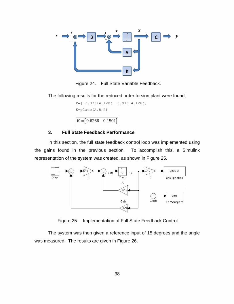
38


The following results for the reduced order torsion plant were found, P=[-3.975+4.128j -3.975-4.128j] K=place(A,B,P)

[ ]0.6266 0.1501K =

3. Full State Feedback Performance

In this section, the full state feedback control loop was implemented using

the gains found in the previous section. To accomplish this, a Simulink

representation of the system was created, as shown in Figure 25.

Figure 25. Implementation of Full State Feedback Control.

The system was then given a reference input of 15 degrees and the angle

was measured. The results are given in Figure 26.

39

0 0.5 1 1.5 2 2.5 30

5

10

15

20

25

30Output of Plant and Controller employing Full State Feedback

Ang

le (

degr

ees)

Time (sec)

Enc 1 Angle

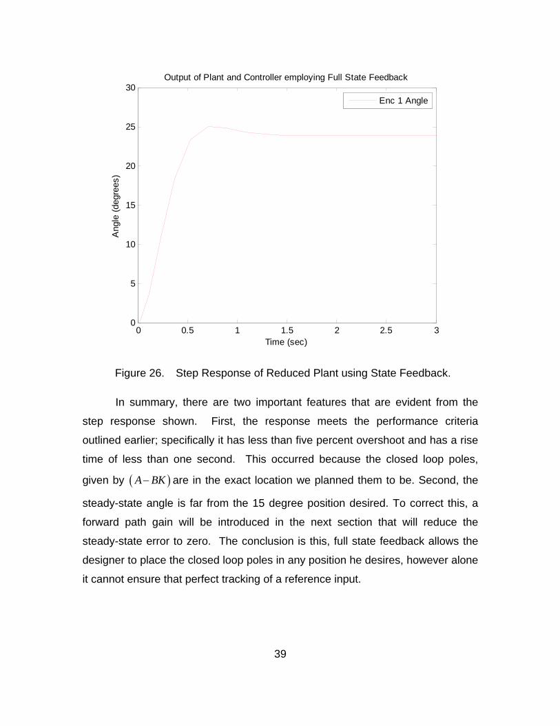
Figure 26. Step Response of Reduced Plant using State Feedback.

In summary, there are two important features that are evident from the

step response shown. First, the response meets the performance criteria

outlined earlier; specifically it has less than five percent overshoot and has a rise

time of less than one second. This occurred because the closed loop poles,

given by ( )A BK− are in the exact location we planned them to be. Second, the

steady-state angle is far from the 15 degree position desired. To correct this, a

forward path gain will be introduced in the next section that will reduce the

steady-state error to zero. The conclusion is this, full state feedback allows the

designer to place the closed loop poles in any position he desires, however alone

it cannot ensure that perfect tracking of a reference input.

40

4. Correcting Steady-state Error: the Forward Path Gain

As already mentioned above, the fault of using full state feedback alone is

that tracking a step input is not guaranteed. To fix this problem, a forward path

gain as shown in Figure 27 is proposed [8].

Figure 27. Full State Feedback with Forward Path Gain.

To show that error tracking a reference input is reduced to zero, let

x Ax Bu= +& (5.7)

where fu K r Kx= − and K = k1 k2 k3[ ]. Substituting above and simplifying,

( ){

clcl

f CL CL

BA

x A BK x BK r A x B r= − + = +&14243

(5.8)

The systems transfer function can be shown to be given by,

( ) ( ) 1( )( )CL CL CL CL CL f

Y sG s C B C SI A BKU s

φ −= = = − (5.9)

If the final value theorem is used and a step input is given as the reference

signal, then

( ){

( )1 1

0( ) ( )( )

( ) lim ( )clcl cl cl f cl cl fs

Y s R sR s

ry sY s sC sI A B K C A B K rs

− −

→∞ = = − = −

144424443 (5.10)

Letting ( ) 15y r∞ = = and solving for fK yields the desired equation

( )11 0.6266

clf cl clK C A B−−⎡ ⎤= − =⎣ ⎦ (5.11)

41

Dutton mentions a word of caution regarding this approach; specifically he

mentions that forward path gains might make the control input voltage to large.

Also, he mentions that the gain is effectively open loop, meaning that any error in

its value would be uncorrected for. An alternative approach would be to form the

output error and add integral control to remove it [8].

5. Full State Feedback with Forward Gain Performance

In this section, the forward path gain is implemented by simply adding a

gain to the Simulink block diagram used for the full state feedback used earlier.

This is shown Figure 28 for ease of reference.

position

enc 1 speed

time

To Workspace

Reference

1s

Plant

K*u

Gain

Kf

Forward gain

Clock

C* u

C

B* u

B

A* u

A

xdot x

Figure 28. State Feedback with Forward Path Gain.

The system’s response to a 15-degree step input is shown in Figure 29.

As before, the state feedback gains ensure the system meets the percent

overshoot and rise time requirements. This time, however, the forward path gain

ensures the system also achieves zero error to a step.

42

0 0.5 1 1.5 2 2.5 30

2

4

6

8

10

12

14

16Output of Plant and Controller employing Full State Feedback and FeedForward

Ang

le (

degr

ees)

Time (sec)

Enc 1 Angle

Steady-State = 15 degrees

Figure 29. Step Response of Reduced Order Plant using State Feedback and

Forward Path Gain.

The full state feedback controller with feed forward gain presented in this

section meets all the performance requirements mentioned earlier. However, full

state feedback controllers require all system states be measurable in order to be

fed back, something very unlikely in practice. In the subsequent section, an

observer will be designed for the reduced order torsion plant that will estimate the

plants angular velocity by only measuring the angle.

B. OBSERVER DESIGN

In situations where the plant states can only be partially measured or it is

cost effective to minimize the number of measured states, the design of a plant

observer to estimate the plants un-measured states can be performed. For the

plant studied in this thesis, an observer design must be considered because the

angular velocity of the lumped disks is not measured directly. In reality only the

angle is measured by means of an encoder.

43

In Chapter IV, it was shown that the plant is completely observable using

only encoder one; thus, a control strategy shown below is proposed where

[ ]1 0C = . In Figure 30, a graphical representation of state feedback using an

observer is given. The hat above the observer states indicate that the states are

estimated, not measured.

Figure 30. State Feedback using an Observer.

1. Effect of Adding an Observer to the Design

In many cases, the designer has no option to use or not to use an

observer; the choice is determined by the inability to measure every state. One

consequence of its implementation, however, is the complexity of the

observer/feedback structure and that the closed loop structure now contains 2n

states (n from the original plant and n from the observer). As noted in [5], this

complexity can be reduced somewhat through the addition of minimum state

observers that take into account that it is unnecessary to estimate states that are

already being measured. Thus, these observers have 2n-m states, where m is

the number of measured states.

44

Another remarkable trait, as noted in [5], is that the feedback and observer

design processes are independent of each other; specifically, the feedback gains

and the observer gains can be designed separately and one does not affect the

other.

In situations when an observer is not required because all states are

measurable, cost might very well make one useful. This is because observers

reduce the number of sensors required to measure states needed for full state

feedback.

2. Calculating the Observer Gains, L

The purpose of the observer is to estimate the actual plant so that even

though the actual states are never measured, the observer’s estimated ones can

be used in the state feedback control. The following theory shows how to

calculate and select observer gains so the observer faithfully estimates the plant.

From the graphical representation above, we can see that

( )ˆ ˆ ˆ ˆ ˆ

x Ax Bu y Cx

x Ax Bu L y y y Cx

= + =

= + + − =

&

& (5.12)

where ˆfu K r Kx= − and [ ]1 2L l l= .

For an observer, our goal is to reduce the error between the actual state

and the estimate to zero.

ˆ 0error x x= − → (5.13)

( )( ) ( )( )ˆ ˆ ˆ ˆe x x Ax Bu Ax Bu L y y A LC x x= − = + − + + − = − −&& & (5.14)

( )e A LC e= −& (5.15)

Thus, the error converges whenever the eigenvalues of ( )A LC− are all

negative. Theoretically, the more negative the eigenvalues, the faster the error

reduces to zero and the more quickly the estimated states converge to the actual

states.

45

In practice, there exists a trade-off between how negative the eigenvalues

can be made and how large the observer gains L are. One typical thumb-rule for

observer design is that the eigenvalues should be 4-10x larger than the desired

closed loop poles discussed earlier ( )1,2 3.975 4.182p j= − ± . To quantify this

notion, an analysis will be presented that compares convergence rate of an

observer using eigenvalues the same magnitude as the closed loop poles to an

observer using eigenvalues ten times father away. To be clear, both cases will

result in observer convergence because the closed loop poles are negative in

both scenarios, but it is expected that the ten times faster poles will converge

faster at the expense of larger observer gains.

Matlab’s PLACE function can again be used to calculate the observer

gains5 for both scenarios mentioned above. The results are shown in Table 1.

Same Order 1,2 3.9p j= − ±

10 X farther Away 1,2 39p j= − ±

7.71 77.9 Observer Gains 15.58 1515

Table 1. Required Observer Gains.

3. Observer Simulation

In this section, a Simulink model of the entire state feedback controller,

using an observer and forward path gain, is shown in Figure 31. The individual

parts of the model have been color coded for ease of reference.

5 K = place(A,B,P) is used to find the gains K that moves the systems poles to those

specified in the vector P. (i.e., P = eig(A-B*K)) Similarly, the command L ‘= place (A’,C’,P) finds the gains L that move the poles to those specified in the vector P. (i.e., P = eig(A-L*C)).

46

Figure 31. Final Control Solution.

For subsequent analysis, it is important to note that since the plant’s

actual initial conditions are rarely known, it was assumed that they started

at[ ]5 .1 T . The observer initial conditions are the best guess at the actual plant’s

initial conditions. Since none are known, [ ]0 0 T was chosen. One benefit of

having the plant and observer start with different initial conditions is that the

observer’s convergence will be easily distinguishable as will be shown in the next

section.

4. Observer Performance

In this section, an analysis of the performance of the observer is

presented. In Figure 32, a comparison of the convergence of the two observers

is shown. The top portion shows the convergence when the observer gains are

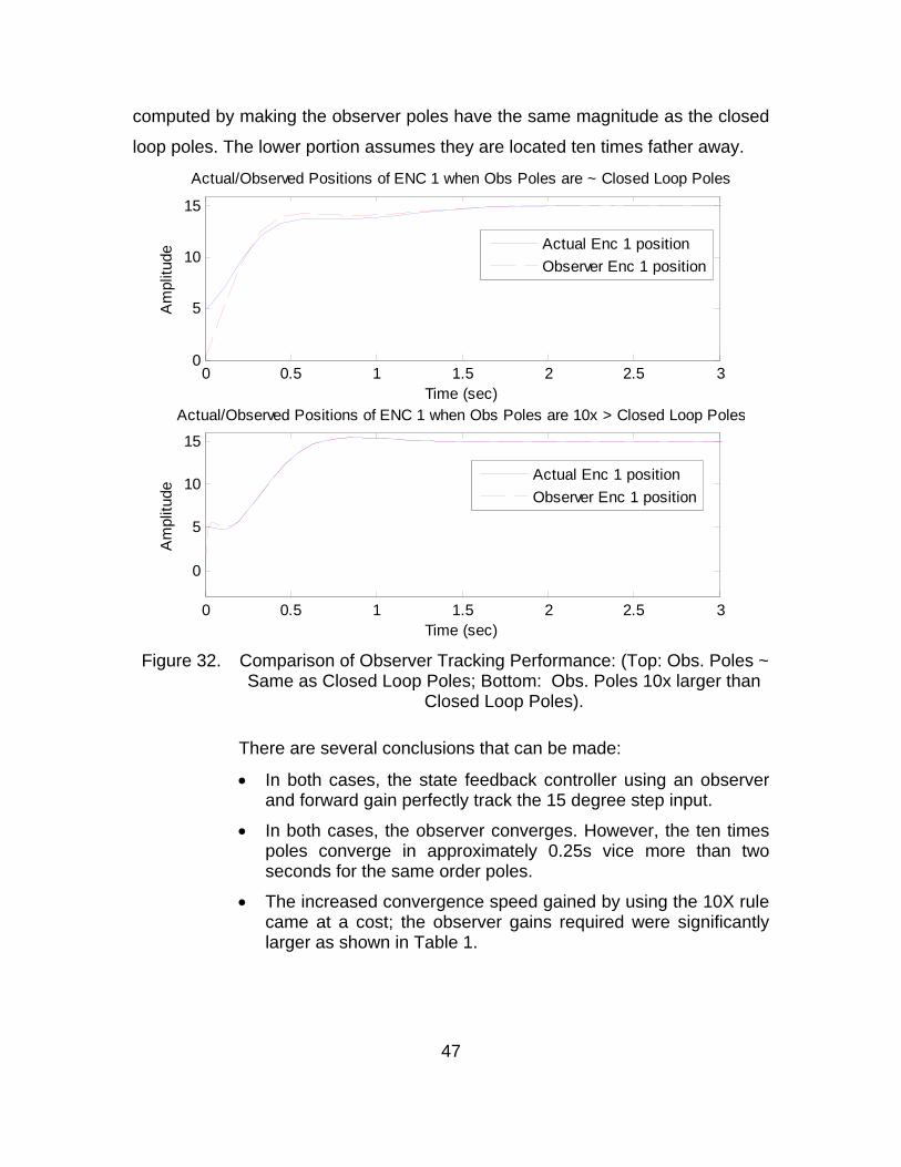
47

computed by making the observer poles have the same magnitude as the closed

loop poles. The lower portion assumes they are located ten times father away.

0 0.5 1 1.5 2 2.5 30

5

10

15

Actual/Observed Positions of ENC 1 when Obs Poles are ~ Closed Loop PolesA

mpl

itude

Time (sec)



0 0.5 1 1.5 2 2.5 3

0

5

10

15

Actual/Observed Positions of ENC 1 when Obs Poles are 10x > Closed Loop Poles

Am

plitu

de

Time (sec)



Figure 32. Comparison of Observer Tracking Performance: (Top: Obs. Poles ~

Same as Closed Loop Poles; Bottom: Obs. Poles 10x larger than Closed Loop Poles).

There are several conclusions that can be made:

• In both cases, the state feedback controller using an observer and forward gain perfectly track the 15 degree step input.

• In both cases, the observer converges. However, the ten times poles converge in approximately 0.25s vice more than two seconds for the same order poles.

• The increased convergence speed gained by using the 10X rule came at a cost; the observer gains required were significantly larger as shown in Table 1.

48

C. SUMMARY

In this chapter, a control strategy for the reduced order torsion plant was

introduced using state feedback via an observer and forward path gain. The final

goal was to be able to move the lumped disks’ angle to any reference in less

than a second and with less than five percent overshoot and have zero error. The

final design used state feedback to meet the performance criteria, a forward path

gain to reduce the steady-state error to a step reference to zero, and an observer

to estimate disks’ angular velocity so that an additional sensor or integration

would not be necessary. In summary, the control strategy was a success and the

objectives met.

49

VI. CONCLUSION AND RECOMMENDATIONS

In this thesis, a state-space approach was used to model, identify and

control a 4th order rotational mechanical system. The key contribution made in

this thesis is summarized in a series of state-space control laboratories detailed

in Appendix A. The goal of these laboratories is to give the student the

opportunity to explore the entire design process from modeling to identification

and finally control.

A. CONCLUSIONS

In conclusion, the key results attained from each chapter of this thesis will

be summarized.

In Chapter II, a free body diagram and electrical model of the torsion plant

were presented. These models aided in applying first principles to the model and

in the derivation of its equations of motion. Finally, the equations were converted

into a 4th order state-space model.

In Chapter III, a parameter estimation method utilized the grey box

structure of the plant to identify unknowns. The 4th order model was then shown

to be rank deficient, an indication that the model contained redundant

information. It was later revealed that this redundancy was due in part to the

rigidity of the shaft coupling the two disks not allowing any appreciable

displacement between the two bodies. Next, a reduced order model was

proposed and subsequently identified. Finally, the reduced order model was

shown to have an accuracy very close to that of the 4th order model.

In Chapter IV, the plant was shown to be stable, having one negative real

pole and another pole at the origin. It was also demonstrated that the reduced

order model was controllable and observable. Controllability was significant

because it signaled that state feedback would succeed in moving the plants

states to any desired location. On the other hand, observability suggested that an

observer could be designed to estimate the plants un-measureable state.

50

In Chapter V, a state feedback controller using an observer and forward

path gain successfully allowed the plant to follow step angle inputs with a rise

time less than one second, less than five percent overshoot and with zero

steady-state error.

Appendix A contains six laboratories that were designed to aid a state-

space control class to repeat the results presented in this thesis. Appendix B

contains the Matlab code used to produce the lab results.

B. RECOMMENDATIONS

There exist several opportunities for further work. First, Educational

Control Products makes a similar rectilinear plant where two masses are

connected, via springs to each other, and controlled by a motor. The benefit of

repeating this work on that model would be that, since there are no rigid shafts

but rather true springs, a complete 4th order model could be identified and

subsequently controlled. This approach might allow for even more insight for

students performing the laboratories.

Educational Control Products also offers an inverted pendulum, which

would lend itself to the development of non-linear controls laboratories. The

state-space model for this plant could be linearized, and either pole placement

design strategy of LQR strategy could be applied.

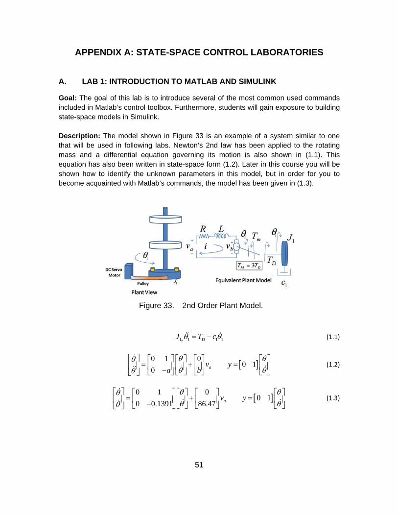
51

APPENDIX A: STATE-SPACE CONTROL LABORATORIES

A. LAB 1: INTRODUCTION TO MATLAB AND SIMULINK

Goal: The goal of this lab is to introduce several of the most common used commands included in Matlab’s control toolbox. Furthermore, students will gain exposure to building state-space models in Simulink. Description: The model shown in Figure 33 is an example of a system similar to one that will be used in following labs. Newton’s 2nd law has been applied to the rotating mass and a differential equation governing its motion is also shown in (1.1). This equation has also been written in state-space form (1.2). Later in this course you will be shown how to identify the unknown parameters in this model, but in order for you to become acquainted with Matlab’s commands, the model has been given in (1.3).

Figure 33. 2nd Order Plant Model.

1 1 1 1T DJ T cθ θ= −&& & (1.1)

[ ]0 1 00 1

0 av ya b

θ θθθ θθ

⎡ ⎤ ⎡ ⎤ ⎡ ⎤ ⎡ ⎤ ⎡ ⎤= + =⎢ ⎥ ⎢ ⎥ ⎢ ⎥ ⎢ ⎥ ⎢ ⎥−⎣ ⎦ ⎣ ⎦ ⎣ ⎦ ⎣ ⎦⎣ ⎦

&

& &&& (1.2)

[ ]0 1 00 1

0 0.1391 86.47 av yθ θθθ θθ

⎡ ⎤ ⎡ ⎤ ⎡ ⎤ ⎡ ⎤ ⎡ ⎤= + =⎢ ⎥ ⎢ ⎥ ⎢ ⎥ ⎢ ⎥ ⎢ ⎥−⎣ ⎦ ⎣ ⎦ ⎣ ⎦ ⎣ ⎦⎣ ⎦

&

& &&& (1.3)

52

Part 1 Converting ss models to transfer functions (ss2tf.m, tf.m, minreal.m)6 Using the state-space model, find the equivalent transfer function representation

[num,den]=ss2tf(A,B,C,D) transfer_function=tf(num,den)

2

86.470.1391

sTFs s

=+

The resulting transfer function can be simplified by using the minimum realization command:

transfer_function =minreal(transfer_function) 86.470.1391

TFs

=+

Part 2 Finding Poles and Zeros (ss2pz.m or eig.m) Using the state-space model, find systems zeros and poles

[z,p,k]=ss2zp(A,B,C,D)

No Zeros; Two Poles: 0,-0.1391 A more common state-space approach is to find the system poles by finding the eigenvalues of the A matrix. This can be accomplished by using the eig.m command.

eig(A) Verify that these approaches yield similar results.

6 Matlab is capable of converting between state-space, transfer function and pole-zero forms

easily; see ss2tf.m, ss2pz.m, tf2pz.m and tf2ss.m (note: converting transfer functions to state-space models are not unique and frequently the meaning of a problems physical variables are lost in the conversion.

53

Part 3 Graphical Representation of Poles/Zeros (pzmap.m) Find a graphical representation of the systems poles and zeros (pzmap.m)

pzmap(A,B,C,D)

-0.14 -0.12 -0.1 -0.08 -0.06 -0.04 -0.02 0-1

-0.8

-0.6

-0.4

-0.2

0

0.2

0.4

0.6

0.8

1Pole-Zero Map

Real Axis

Imag

inar

y A

xis

Figure 34. Pole Zero Map.

Part 4 Simulations (initial.m , lsim.m, step.m, impulse.m) In order to practice with the various simulation commands in Matlab, two data files are given to you. The first file below contains experimental angle data when 0.15 volts are applied to the motor. The second file contains angle data when no input is applied but the disk is given an initial offset of 10 degrees.

point15volts_50sec_1disk_2mass.txt no_voltage_10_degree_angle_ic.txt

The lsim.m command is probably the most powerful of the above commands in that it simulates the plant with any arbitrary input, with or without initial conditions and plots the response. Assume that the motor has 0.15 volts applied (constant step) and that it starts from rest with no initial angle. (initial conditions = 0). Use lsim.m to simulate the state-

54

space model and plot the response. Then overlay the given experimental data and comment on how well the model works. Note: the actual system requires a minimum of 0.0774V to overcome friction and begin to move. This is known as the system dead-zone. The dead-zone will be explained in more detail in lab 3. For now, assume the actual voltage that speeds up the shaft is V_dz = 0.15 - 0.0774. Also there are 1600 encoder counts for every 2π rad. C=[1 0]; Vdz=.0774; input=(0.15-Vdz)*ones(5001,1); X0=[10;0]; T=0:.01:50; lsim(A,B,C,D,input,T,X0) hold on load -ASCII point15volts_50sec_1disk_2mass.txt time = point15volts_50sec_1disk_2mass(:,2) position=point15volts_50sec_1disk_2mass(:,3)*(2*pi/16000) plot(time,position) This plot could also have been produced using the step.m as follows [y,t] = step(A,B,C,D) plot(t,(0.15-Vdz)*y) Use Initial.m to plot the initial condition response of the system. For this plot, assume disk one is displaced 10 degrees and then let go. Be sure to set C= [1 0] to generate how the angle varies. On the same plot, overlay and compare this to the given data above to see how accurate the state-space model is. load -no_voltage_10_degree_angle_ic.txt time = point15volts_50sec_1disk_2mass(:,2) position=point15volts_50sec_1disk_2mass(:,3) X0=[10;0]; initial(A,B,C,D,X0) hold on title('Use of Initial Command to Verify Model Validity for IC') plot(time,position) legend('Simulation Response','Experimental Response')

55

Table 2. Table of Common State-space Matlab Commands (After [9])

Command Description acker Compute the K matrix to place the poles of A-BK, see also place

c2dm Continuous system to discrete system ctrb The controllability matrix, see also obsv

det Find the determinant of a matrix eig Compute the eigenvalues of a matrix

impulse Impulse response of continuous-time linear systems inv Find the inverse of a matrix

lsim Simulate a linear system obsv The observability matrix, see also ctrb

ones Returns a vector or matrix of ones place Compute the K matrix to place the poles of A-BK, see also acker

pzmap Pole-zero map of linear systems rank Find the number of linearly independent rows or columns of a

matrix roots Find the roots of a polynominal

ss Create state-space models or convert LTI model to state-space ss2tf State-space to transfer function representation

ss2zp State-space to pole-zero representation step Plot the step response

tf Creation of transfer functions or conversion to transfer function tf2ss Transfer function to state-space representation

tf2zp Transfer function to Pole-zero representation zp2ss Pole-zero to state-space representation

zp2tf Pole-zero to transfer function representation

Note: The table is adapted from http://www.engin.umich.edu/group/ctm/extras/commands.html.

56

Simulink Simulink is a graphical extension of Matlab used in the simulations of systems. Transfer functions and state-space models can be implemented visually by means of block diagrams. In this section, the basic foundation of how to build a state-space model in Matlab will be introduced as well as how to simulate the model with and without initial conditions just as was done earlier using matlab alone. To open Simulink, simply type simulink from the command line in Matlab. The Simulink Library Browser should appear in a separate window. As can be seen in the library, elements of block diagrams are organized by type (Continuous, Discrete, Sources, Sinks etc.) Our goal is to build the state-space model for the plant given earlier. A graphical representation of the complete diagram is shown in Figure 35. The diagram also contains information about where in the library to find the specified blocks. Building the Model

• Open Simulnk: Type Simulink on the command line in matlab. • Open a new model. Select File, New model • Create an m-file in matlab and define the A,B,C,D matrix’s given earlier.7 • Find and drag the elements shown to your model window. To connect elements

simply drag the output of the desired block to the input of the corresponding element.

• Double clicking the elements name allows you to change the objects name as well as change parameters. Change each element according to the graphic

7 If the model is saved in the same folder as the m-file, then once the m- file is run the

variables stored in the workspace will be available to Simulink. Similarly, once the model is run, its parameters are available in Matlab.

57

Figure 35. Simulink Model Building.

Simulating the Model

• Set the simulation time to be 50 seconds by: 50Simulation Configuration Parameters Stop Time→ → =

• Run the identification.m file so that [A, B, C, D] are in the workspace • Run the simulation by clicking the start icon in Simulink or typing

sim(‘simulink_file_name’) in matlab • Velocity and Time variable vectors should be created in matlab.

Plot and Compare the Simulation Results vs Experimental Results in Matlab Given the experimental_data.txt file which contains actual experimental data found by inputting the above plant with 0.15V, graph and compare this with your simulation results as shown below.

• Import Experimental Velocity Data load -ASCII velocity.txt exp_time=velocity(:,2) exp_velocity=velocity(:,3)

• Plot Simulation and Experimental together

plot(exp_time,exp_velocity,’r’,time,velocity,’b’) legend(‘Experimental Results’,’Simulation Results’) title(‘Comparison of Experimental and Simulation’)

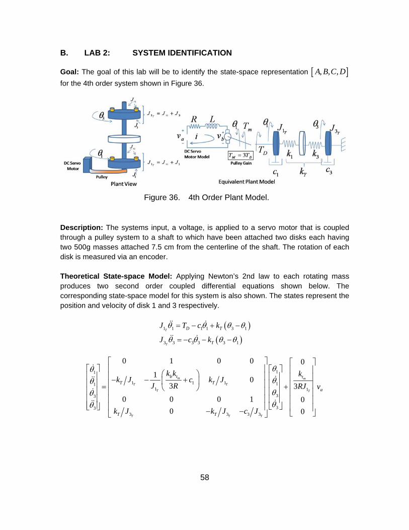
58

B. LAB 2: SYSTEM IDENTIFICATION

Goal: The goal of this lab will be to identify the state-space representation [ ], , ,A B C D for the 4th order system shown in Figure 36.

Figure 36. 4th Order Plant Model.

Description: The systems input, a voltage, is applied to a servo motor that is coupled through a pulley system to a shaft to which have been attached two disks each having two 500g masses attached 7.5 cm from the centerline of the shaft. The rotation of each disk is measured via an encoder. Theoretical State-space Model: Applying Newton’s 2nd law to each rotating mass produces two second order coupled differential equations shown below. The corresponding state-space model for this system is also shown. The states represent the position and velocity of disk 1 and 3 respectively.

( )( )

1 1 1 1 3 1

3 3 3 3 3 1

T

T

D T

T

J T c k

J c k

θ θ θ θ

θ θ θ θ

= − + −

= − − −

&& &

&& &

11

1 1 1 111 1

33

333 3 3 3

0 1 0 0 01 0

3 30 0 0 1 0

0 0

m m

T T

T T

T T T

b t tT T

a

T T

k k kk J c k J

J R RJ v

k J k J c J

θθθθθθθθ

⎡ ⎤ ⎡ ⎤⎡ ⎤ ⎢ ⎥ ⎡ ⎤ ⎢ ⎥⎛ ⎞⎢ ⎥ ⎢ ⎥ ⎢ ⎥ ⎢ ⎥− − +⎜ ⎟⎢ ⎥ ⎢ ⎥ ⎢ ⎥ ⎢ ⎥= +⎝ ⎠⎢ ⎥ ⎢ ⎥ ⎢ ⎥ ⎢ ⎥⎢ ⎥ ⎢ ⎥ ⎢ ⎥ ⎢ ⎥⎢ ⎥ ⎣ ⎦⎣ ⎦ ⎢ ⎥ ⎢ ⎥− − ⎣ ⎦⎣ ⎦

&

&&&

&

&&&

59

Part 1: Experimentally Determining the Systems Dead-Zone A dead-zone refers to the range of voltages that, if applied to the system, do not result in moving the shaft because they are not great enough to overcome the systems friction. This dead-zone is the primary culprit for the nonlinear behavior of system and if it can be identified first, techniques in the next part of this lab can be used to identify the remaining linear portion. Our final model will then include two pieces, a dead zone and the linear portion. To identify the dead zone we need to find the first voltage that causes the shaft to move. To do this we will start by applying a step voltage of 0.15 V and measure the corresponding steady-state speed of the shaft. Next we will decrease this voltage in 0.01V intervals and after taking three successive measurements the dead-zone voltage will be found through extrapolation as shown in Figure (37).

0 0.02 0.04 0.06 0.08 0.1 0.12 0.14 0.160

5

10

15

20

25

30

35

40

45

50Final Velocity vs Applied Voltage

Applied Voltage (V)

Fin

al V

eloc

ity (

Rad

/sec

)

y = 648*x - 52.9

Dead Zone Voltage

Figure 37. Extrapolation to Find Dead-zone.

Collecting Experimental Data Steps: 1. Open the ECP Software

2. Change the method that the ECP software displays units Setup → User Units → Degrees

The following steps are used to input a 0.15 V step and record the output angle of both disks 1, 3 for 50 seconds

60

3. Turn ECP Controller Power ON

4. Command Menu → Trajectory→ Select Impulse

5. Select Open Loop Impulse → Amplitude = 0.15 V → Pulse Width =

1000ms→ 5 repetitions→ Dwell time = 0 s → OK→ OK8

6. Data Menu → select Encoder #1 and Encoder #3 → Select OK The program is now ready to acquire data when executed. 7. From Utility Menu→ Zero Position (zeros encoder positions)

8. From Command Menu→ Select Execute

9. From Plotting Menu→ Select Set-up Plot→ Choose Encoder 3 Velocity

→ Plot Data

10. Verify that the velocity data reaches steady-state.

Next the data should be stored so that it can be imported into Matlab.

11. Data→ Export Raw Data→ Save Data as: point15volts.txt

12. Repeat steps 5-12 for input voltages of 0.14V, 0.13V

13. Open each text file and erase each column header (but remember what each

column contains). This is done so that the data can be imported into Matlab.

14. Import the three data files into a Matlab m-file in the following manner,

load -ASCII point15volts.txt

15. Calculate the shafts velocity for each case from the measured position position_delta=diff(point15volts(:,3)); time_delta=diff(point15volts(:,2));

velocity=position_delta / mean(time_delta);

16. Convert the velocity from counts revolution to srad 9 Velocity=velocity*(2*pi/16000);

17. Find the final steady-state shaft velocities for each of the three cases either by plotting the velocity vs. time profile or looking at the end of the velocity vector.

8 The ECP software step input command is configured to provide a step followed by an equal

duration zero signal. Since the zero signal is not desired, a work around is used via the impulse signal as desired above.

9 There are 16000 encoder counts per revolution.

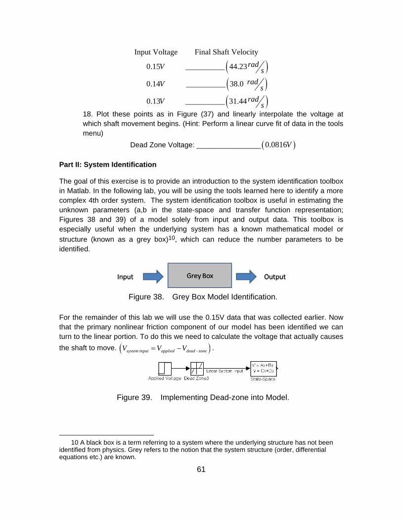
61

( )( )( )

Input Voltage Final Shaft Velocity

0.15 __________ 44.23

0.14 __________ 38.0

0.13 __________ 31.44

radV sradV sradV s

18. Plot these points as in Figure (37) and linearly interpolate the voltage at which shaft movement begins. (Hint: Perform a linear curve fit of data in the tools menu) Dead Zone Voltage: ________________ ( )0.0816V

Part II: System Identification The goal of this exercise is to provide an introduction to the system identification toolbox in Matlab. In the following lab, you will be using the tools learned here to identify a more complex 4th order system. The system identification toolbox is useful in estimating the unknown parameters (a,b in the state-space and transfer function representation; Figures 38 and 39) of a model solely from input and output data. This toolbox is especially useful when the underlying system has a known mathematical model or structure (known as a grey box)10, which can reduce the number parameters to be identified.

Figure 38. Grey Box Model Identification.

For the remainder of this lab we will use the 0.15V data that was collected earlier. Now that the primary nonlinear friction component of our model has been identified we can turn to the linear portion. To do this we need to calculate the voltage that actually causes the shaft to move. ( )system input applied dead zoneV V V −= − .

Figure 39. Implementing Dead-zone into Model.

10 A black box is a term referring to a system where the underlying structure has not been

identified from physics. Grey refers to the notion that the system structure (order, differential equations etc.) are known.

62

A: Find this voltage: _____________ System Identification Procedure Part 2.1 Importing Input/Output Data into Matlab

• Open Matlab and open a new m-file. (File - New - M-file) • Clear all variables and close all open windows (clear all, close all) • Create or import the velocity data vector for the 0.15V input case above • Create the systems input as a vector of constant voltages equal to the input

volate found in A above. The length of this vector should be the same as that of the output (input=system_input_voltage*ones(length(velocity), 1)

Part 2.2 Constructing Data Structures in Matlab

• The identification toolbox identifies model parameters from data stored in a specific format known as an iddata structure. The matlab call to create this structure is:

data = iddata(output,input,Ts)

where Ts is the sampling time at which the data was taken. To find this you can take the experiment time (50 sec) and divide that by number of measurements (i.e. the length of the data vector). Assume this has been done for you Ts = .0089

Part 2.3 Constructing a Continuous-Time State-Space Model Object A state-space model object is similar to a storage unit that contains all the information about a state-space model. It not only contains the state-space model but has the ability for the user to specify parameters that are going to be estimated from given data. Creating a state-space model is done using:


• Setting up the model object is done in three steps, first we define a nominal parameter model inserting in only the known entries.12 Second we create the object, and third we specify which entries in the model we desire matlab to do parametric analysis on. These steps are shown below.

11 Continuous and Discrete state-space model can be stored as objects. To distinguish the

two, the sampling time is set to zero in the continuous model. 12 The continuous time state-space representation in matlab includes a noise term which

should be set to zero. x Ax Bu Kw y Cx Du w= + + = + +&

63

Defining a nominal model13: insert only the known entries.

A = [0 1 0 0 ; 0 0 0 0;0 0 0 1;0 0 0 0]; B = [0 0 0 0]'; C = [0,1,0,0]; D = 0; K = zeros(4,1); x0 = [0;0;0;0];

Create the model object using


Specifying Parameters to be Estimated

Run the above m-file and at the matlab prompt type get(m).15 This shows the properties of the stored object. Notice that in the middle of the object there exists other data areas that can be used in parameterization. It is those structures that we will used to tell matlab which entries in our model are parameters to be identified. SSParameterization: 'Structured' As: [4x4 double] Bs: [4x1 double] Cs: [0 1 0 0] Ds: 0 Ks: [4x1 double] X0s: [4x1 double] To specify which parameters are to be estimated, the NaN characters are used as shown below:

m.As = [0 1;0,NaN]; m.Bs = [0 NaN]'; m.Cs = [0 1]; m.Ds = 0; m.Ks = m.k; m.x0s = [0;0];

13 Unknown values in the model (i.e. a,b) should be initialized with best guesses. If unknown, zero should be used.

14 Continuous and Discrete state-space model can be stored as objects. To distinguish the two, the sampling time is set to zero in the continuous model.

15 Individual entries of the structure can be seen by entering m.(desired entry) at the matlab prompt.

64

Part 2.4 Perform Parameter Estimation

1. Matlab has a tool for parameter estimation upon state-space objects known as pem.m, which requires both data (output data structure) from step 5 and the state-space model object (m) from step 7. It can be implemented as follows:

m =pem(data,m) Part 2.5 Extracting the State-space Model

2. The state-space model can be extracted from the m object structure by

[A,B,C,D]=ssdata(m) Write the final state-space model below The state-space model for the system is

[ ]5

0 1 0 0 01.605 10 .0756 0 0 49.9655

0 1 0 00 0 0 1 00 0 0 0 0

xA B C

−

⎡ ⎤ ⎡ ⎤⎢ ⎥ ⎢ ⎥− −⎢ ⎥ ⎢ ⎥= = =⎢ ⎥ ⎢ ⎥⎢ ⎥ ⎢ ⎥⎣ ⎦ ⎣ ⎦

Congratulations! The systems state-space model has now been identified from input/out data!

65

C. LAB 3: MODEL VERIFICATION

Goal: The goal of this lab is to verify that the state-space model built previously matches the experimental results found in the laboratory. To do this, a state-space model will be built in Simulink that incorporates the non-linear dead zone as well as our estimated plant model. This model will be simulated with 0.15 V, 0.14 V and 0.13 V in the same manner as was done to the actual system in the lab. The outputs will then be compared and the accuracy of the modeled assessed. Part 1: Building the Simulink Model Step 1: Open Simulink and Open a New Model Step 2: Build the Model shown in Figure 40.

Figure 40. Simulink Model Building.

Step 3: Open the m-file from lab 1 that contains:

a. The velocity response vectors when 0.15V, 0.14V, 0.13V b. The dead zone voltage c. The estimated state-space model

Step 4: Run the Simulink file for each input.16

16 A Simulink model can be run directly from a Matlab m-file if saved in same directory using

the command: sim('State Space Model Name')

66

Step 5: Make a plot comparing the experimental results against the simulated model results similar to the one in Figure 41. Comment on the accuracy of the model.

0 5 10 15 20 25 30 35 40 45 500

5

10

15

20

25

30

35

40

45

Time (s)

Vel

ocity

Dis

k 1

(rad

/s)




0 5 10 15 20 25 30 35 40 45 500

5

10

15

20

25

30

35

Time (s)

Vel

ocity

Dis

k 1

(rad

/s)




0 5 10 15 20 25 30 35 40 45 500

2

4

6

8

10

12

14

16

18

20

Time (s)

Vel

ocity

Dis

k 1

(rad

/s)




0 5 10 15 20 25 30 35 40 45 50-2

0

2

4

6

8

10

12

14

Time (s)

Vel

ocity

Dis

k 1

(rad

/s)




Figure 41. Model Verification.

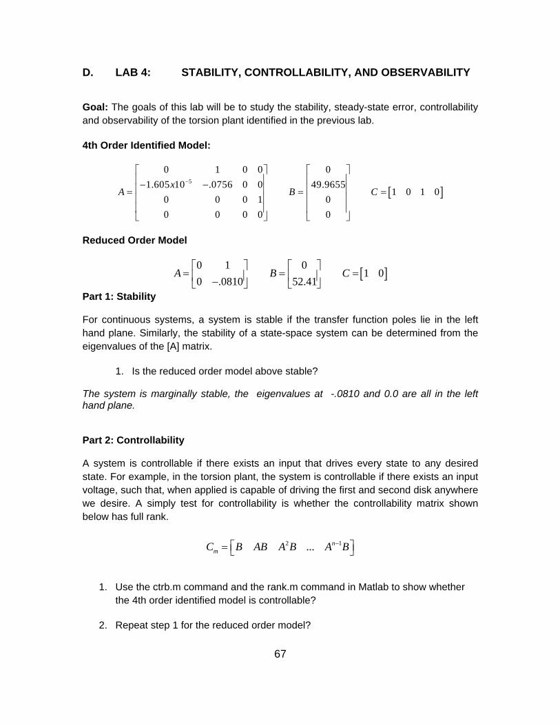
67

D. LAB 4: STABILITY, CONTROLLABILITY, AND OBSERVABILITY

Goal: The goals of this lab will be to study the stability, steady-state error, controllability and observability of the torsion plant identified in the previous lab. 4th Order Identified Model:

[ ]5

0 1 0 0 01.605 10 .0756 0 0 49.9655

1 0 1 00 0 0 1 00 0 0 0 0

xA B C

−

⎡ ⎤ ⎡ ⎤⎢ ⎥ ⎢ ⎥− −⎢ ⎥ ⎢ ⎥= = =⎢ ⎥ ⎢ ⎥⎢ ⎥ ⎢ ⎥⎣ ⎦ ⎣ ⎦

Reduced Order Model

[ ]0 1 01 0

0 .0810 52.41A B C⎡ ⎤ ⎡ ⎤= = =⎢ ⎥ ⎢ ⎥−⎣ ⎦ ⎣ ⎦

Part 1: Stability For continuous systems, a system is stable if the transfer function poles lie in the left hand plane. Similarly, the stability of a state-space system can be determined from the eigenvalues of the [A] matrix.

1. Is the reduced order model above stable?

The system is marginally stable, the eigenvalues at -.0810 and 0.0 are all in the left hand plane.

Part 2: Controllability A system is controllable if there exists an input that drives every state to any desired state. For example, in the torsion plant, the system is controllable if there exists an input voltage, such that, when applied is capable of driving the first and second disk anywhere we desire. A simply test for controllability is whether the controllability matrix shown below has full rank.

2 1... nmC B AB A B A B−⎡ ⎤= ⎣ ⎦

1. Use the ctrb.m command and the rank.m command in Matlab to show whether the 4th order identified model is controllable?

2. Repeat step 1 for the reduced order model?

68

Can you think of a reason why one model would be controllable while the exact same higher order model is not? In other words, why is it not possible to find an input that drives disk one to 15 degrees and disk two to 30 degrees simultaneously? The reason the 4th order model’s controllability matrix is rank deficient is that the shaft that connects the two masses is not flexible enough to exhibit a spring-like behavior. In reality, the difference in angle between the disks is extremely small. Thus from the perspective of the input motor, the two disk separated by a shaft disks appear to be a single disk moving at one speed. Part 4: Observability Observability refers to the ability to estimate a systems state that cannot be measured from our output. For example, if the two disk system used in this lab is observable that would infer that we could estimate the position of the second disk given only a measurement of disk one. A simply test for observability is whether the observability matrix shown below has full rank.

2 1...Tn

mO C CA CA CA −⎡ ⎤= ⎣ ⎦

1. Without calculating the observability matrix for the 4th order model, do you expect to be able to estimate the position of the second disk from the first?

Theoretically, the 4th order model is in fact not observable because it is impossible for the output to see the second state. However, in reality, because the disks are structurally fixed by the shaft, the input is able to touch both states.

2. Calculate the observability of the reduced order model. From this results do you expect that we can estimate the angular velocity of disks without any sensors? (only from angle measurements.)

Note: In the next lab, a pole placement control strategy will be employed to move the systems poles in such a manner that when a 1 degree rotation of disk one is command, the system will rotate 1 degree with less than 5% overshoot and have a rise time less than 1 second. Since the system is not controllable, we will not concern ourselves with attempting to move the disks to two separate positions. Thus for all future work we will avail ourselves of the reduced order model.

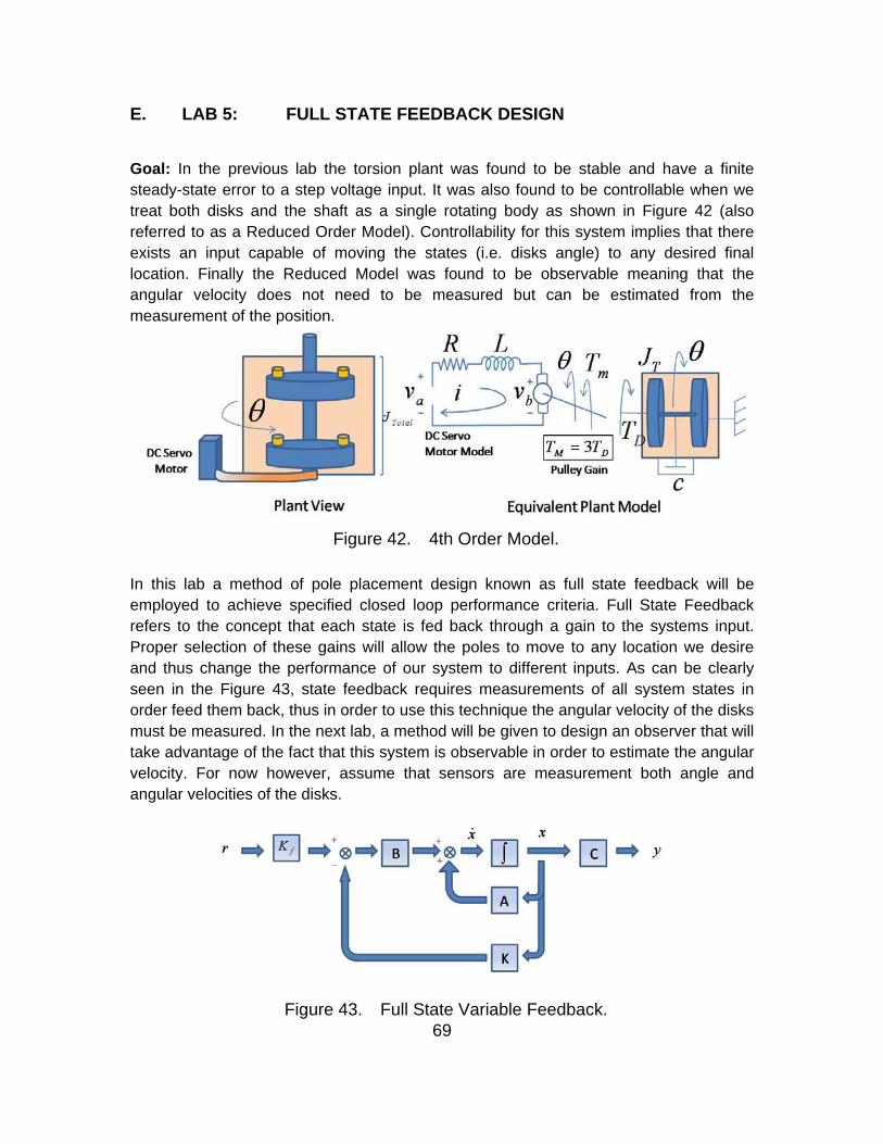
69

E. LAB 5: FULL STATE FEEDBACK DESIGN

Goal: In the previous lab the torsion plant was found to be stable and have a finite steady-state error to a step voltage input. It was also found to be controllable when we treat both disks and the shaft as a single rotating body as shown in Figure 42 (also referred to as a Reduced Order Model). Controllability for this system implies that there exists an input capable of moving the states (i.e. disks angle) to any desired final location. Finally the Reduced Model was found to be observable meaning that the angular velocity does not need to be measured but can be estimated from the measurement of the position.

Figure 42. 4th Order Model.

In this lab a method of pole placement design known as full state feedback will be employed to achieve specified closed loop performance criteria. Full State Feedback refers to the concept that each state is fed back through a gain to the systems input. Proper selection of these gains will allow the poles to move to any location we desire and thus change the performance of our system to different inputs. As can be clearly seen in the Figure 43, state feedback requires measurements of all system states in order feed them back, thus in order to use this technique the angular velocity of the disks must be measured. In the next lab, a method will be given to design an observer that will take advantage of the fact that this system is observable in order to estimate the angular velocity. For now however, assume that sensors are measurement both angle and angular velocities of the disks.


70

The diagram above also contains a forward path gain that will be used to reduce the steady-state error, as we will show shortly. Pre-lab: Finding Desired Transfer Function The goal of this design is for the torsion plant to be capable of moving to within 98% of any desired reference angle in 1 second with less than 5% overshoot in the process. These criteria are summarized below:

Given: 1sT = second; % % 5%Overshoot OS= = 1. Using the equation provided, calculate the required damping ratio

( )( )

( )( )2 2 2 2

ln % /100 ln 5 /100.689

ln % /100 ln 5 /100

OS

OSξ

π π

− −= = =

+ +

2. Using the equation provided, calculate the systems natural frequency

( )( )4 4 4 5.77

.6925 1s nn s

TT

ωξω ξ

= ⇒ = = =

3. Using the standard form of a second order system, find the desired transfer

function 2

2 2 2

33.29( )2 7.95 33.29

ndesired

n n

G ss s s s

ωξω ω

= =+ + + +

4. Find the roots of the desired transfer function.

1,2 3.975 4.182p j= − ±

The desired transfer function has pole location that we need our closed loop system to

have in order to attain the performance criteria outlined above.

71

Part 1: Full State Feedback Design


The closed loop system of the state-space system x Ax Bu= +& where fu K r Kx= − is given by

( ) f CL CLx A BK x BK r A x B r= − + = +&

The main idea here is to see that the presence of state feedback has changed the closed loop poles (the eigenvalues of A) to any desired position we desire simply by correctly choosing the gains

[ ]1 2K k k=

1. In matlab, define a vector P that contains the desired system poles found in the pre-lab.

P=[-3.975+4.128j -3.975-4.128j]

2. Use the place.m command and the reduced order model of the torsion plant (given below) to find the gains K that move our poles to the desired position.

K=place(A,B,P) [ ]0.6266 0.1501K =

3. Implement this control scheme in Simulink, as shown in Figure 45, and plot the disk angle response to a step input of 15 degrees. From your graph, what is the ss-error to this step?

72

Figure 45. Plant with State Feedback’s Step Response.

State Feedback alone only moves the poles to achieve the performance criteria above, it does not address the issue of steady-state error. Next we show how a forward path gain solves this. Part II: Forward Path Gain to Reduce Steady-state Error The forward path required to reduced the steady-state error to zero is given by:

( )11

clf clK C A B−−⎡ ⎤= − ⎣ ⎦

where andCL CL fA A BK B BK= − = 1. Using Matlab, calculate the forward path gain required to drive the error to a 15

degree step to zero.

A_cl=A-B*K B_cl=B;

Kf=-inv(C*inv(A_cl)*B_cl)

0.6266fK = 2. Update your full-state feedback Simulink model to include the forward path gain.

Again, plot the response to a 15 degree step. Did the gain drive the steady-state error to zero?

Figure 46. Plant with State Feedback and Forward Gain’s Step Response.

73

F. LAB 6: OBSERVER DESIGN

Description In situations where the plants states can only be partially measured or it is cost effective to minimize the number of measured states, a plant observer can be used to estimate unmeasured states. The goal of this lab will be to design an observer to estimate the angular velocity the torsion plant. The final closed loop plant will utilize both state feedback and an observer as shown in Figure 47.

Figure 47. Graphical Representation of Pole Placement Design using an Observer.

The methodology is as follows, first a gain L will be found such that the observer’s estimated states closely follow the actual states, next the feedback gains K found in lab 5 will be used to multiple the estimated states instead of the actual states since in reality only the disk angle and not the angular velocity will be measured. As before, the forward path gain will be used to drive the error to zero.

74

Part 1: Observer Gains The structure of the model above is given by

( )ˆ ˆ ˆ ˆ ˆ

x Ax Bu y Cx

x Ax Bu L y y y Cx

= + =

= + + − =

&

& Where, ˆfu K r Kx= − and [ ]1 2 3L l l l= . For an observer, our goal is to reduce the

error between the actual state and the estimate to zero. ˆ 0error x x= − → (1.4)

( )( ) ( )( )ˆ ˆ ˆ ˆe x x Ax Bu Ax Bu L y y A LC x x= − = + − + + − = − −&& & (1.5)

( )e A LC e= −& (1.6)

Thus the error converges whenever the eigenvalues of ( )A LC− are all negative.

1. Use the place.m17 command in Matlab to calculate the observer gains required to reduce the error between the plant and estimated states to zero. First assume that the observer poles are the same as the actual poles. Then assume that they are 10x the actual poles.

L=place(A',C',Observer_Poles) L=L'

Same Order as Actual

1,2 3.9p j= − ± 10 X Actual Order

1,2 39p j= − ± Observer Gains 7.71 77.9 Observer Gains 15.58 1515

2. Build the Simulink of the Plant and Observer shown in Figure 48. Since the

plants actual initial conditions are rarely known, let them start at [ ]5 .1 T . The

observer initial conditions should be your best guess at the actual plants initial

conditions. Since none are known, choose[ ]0 0 T .

17 K = PLACE(A,B,P) is used to find the gains K that moves the systems poles to those

specified in the vector P. (i.e. P = eig(A-B*K)) Similarly, the command L ‘= PLACE (A’,C’,P) finds the gains L that move the specified poles to those specified in the vector P. (i.e. P = eig(A-L*C)).

75

plant_states

To Workspace2

time1

To Workspace1

observer_states

To Workspace

Reference1

1s

Plant1

1s

Plant

L* u

L

Kf

Forward gain1

K*u

Feedback

Clock1

C* u

C1

C* u

C

B* u

B1

B* u

B

A* u

A1

A* u

A

xdot x measured output

x_hat_dot x_hat y _hat

Figure 48. Simulink Implementation of the Controller/Observer.

3. Compare the actual angle and estimated angle when a 15 degree step input is introduced. Assume that the observer gains, L, found by using the same order as actual rule are used. How long does convergence take?

4. Compare the actual angle and estimated angle when a 15 degree step input is introduced. Assume that the observer gains, L, found by using the 10x rule are used. How long does convergence take now?

5. Using the 10x rule gains, change the reference to be a 10 Hz sinusoid at 40 Hz.

Compare the tracking performance to before.

76

0 0.5 1 1.5 2 2.5 3

-2

0

2

4

6

8

10Actual/Observed Positions of ENC 1 when Obs Poles are 10x > Dominant Poles

Am

plitu

de

Time (sec)



Figure 49. Observer Convergence for a Sinusoidal Input.

The performance of the observer appears unaffected. I believe the convergence rate of the error is dependent solely on the observer pole locations and not the input signal. This result was unexpected.

77

APPENDIX B: MATLAB CODE

MATLAB CODE (LAB 1-6)

Lab 1 Matlab Intro clear all close all Define State Space Model A=[0 1;0 -.1391]; B=[0;86.4689]; C=[0 1]; D=[0]; Part 1 Convert SS to tf model [num,den]=ss2tf(A,B,C,D) transfer_function=tf(num,den) transfer_function_min=minreal(transfer_function) num = 0 86.4689 0 den = 1.0000 0.1391 0 Transfer function: 86.47 s -------------- s^2 + 0.1391 s Transfer function: 86.47 ---------- s + 0.1391 Part 2 Find Poles and Zeros [z,p,k]=ss2zp(A,B,C,D) eig(A) z = 0

78

p = 0 -0.1391 k = 86.4689 ans = 0 -0.1391 Part 3 Graphical representation of zeros/poles figure(1) pzmap(A,B,C,D) Part 4 Simulations % 1. Comparing Simulation and Experimental Response to 0.15 V input figure(3) C=[1 0]; Vdz=.0774; input=(0.15-Vdz)*ones(5001,1); X0=[10;0]; T=0:.01:50; lsim(A,B,C,D,input,T,X0); hold on load -ASCII point15volts_50sec_1disk_2mass.txt time = point15volts_50sec_1disk_2mass(:,2); position=point15volts_50sec_1disk_2mass(:,3)*(2*pi/16000); plot(time,position) title('Use of LSIM Command to Verify Model Validity ') plot(time,position) legend('Simulation Response','Experimental Response') % 2. Comparing Initial Condition Response to Experimental load -no_voltage_10_degree_angle_ic.txt time = point15volts_50sec_1disk_2mass(:,2) position=point15volts_50sec_1disk_2mass(:,3) figure(2) X0=[10;0]; initial(A,B,C,D,X0) hold on title('Use of Initial Command to Verify Model Validity for IC') plot(time,position) legend('Simulation Response','Experimental Response')

79

Lab 2: Part 1 Find System Dead Zone clear all close all Part 1.1 Find the Entire Systems Dead Zone % This program has been modified to plot the velocity vs applied voltage automatically if data is given; % All user needs to do to get deadzone voltage is do a curve fit and find y-intercept trials=4; %total # of data sets Part 1.14 Import Angles Data into Matlab load -ASCII point10volts_50sec_2disk_2mass.txt load -ASCII point11volts_50sec_2disk_2mass.txt load -ASCII point13volts_50sec_2disk_2mass.txt load -ASCII point15volts_50sec_2disk_2mass.txt applied_voltage=[.10 .11 .13 .15]; Part 1.15 Convert Angle Data to Ang Velocity Data pos(:,1)=point10volts_50sec_2disk_2mass(:,3); pos(:,2)=point11volts_50sec_2disk_2mass(:,3); pos(:,3)=point13volts_50sec_2disk_2mass(:,3); pos(:,4)=point15volts_50sec_2disk_2mass(:,3); time(:,1)=point10volts_50sec_2disk_2mass(:,2); time(:,2)=point11volts_50sec_2disk_2mass(:,2); time(:,3)=point13volts_50sec_2disk_2mass(:,2); time(:,4)=point15volts_50sec_2disk_2mass(:,2); n=length(point10volts_50sec_2disk_2mass); Part 1.15/1.16 Also convert to rad/s for k=1:trials position_delta(:,k)=diff(pos(:,k)); time_delta(:,k)=diff(time(:,k)); velocity(:,k)=(position_delta(:,k)./time_delta(:,k)) *(2*pi/16000); end Part 1.17 Find SS Shaft Velocity and Plot Them for i=1:trials ave_vel_f(i)=mean(velocity(length(velocity)-30:end,i)); end figure(1) plot(applied_voltage,ave_vel_f,'*') title('Final Velocity vs Applied Voltage') xlabel('Applied Voltage (V)') ylabel('Final Velocity (deg/sec') axis([0 .16 0 50])

80

Lab 3 Intro to Simulink and Model Verification clear all close all Part 1.1 Open Simulink State-Space Model Part 1.2 Build Simulink State-Space Model (see model below) Part 1.3

a. Import Experimental Position Data and Convert to Velocity

%%Load Experimental Angle Data (2 disk / 2 weights) load -ASCII point15volts_50sec_2disk_2mass.txt % This file contains the experimental simulation data (entire plant .15V) load -ASCII point13volts_50sec_2disk_2mass.txt % This file contains the experimental simulation data (entire plant .13V) load -ASCII point11volts_50sec_2disk_2mass.txt % This file contains the experimental simulation data (entire plant .11V) load -ASCII point10volts_50sec_2disk_2mass.txt % This file contains the experimental simulation data (entire plant .10V)

Convert Experimental Angle Data to Ang Velocity Data model_test=point15volts_50sec_2disk_2mass; model_test2=point13volts_50sec_2disk_2mass; model_test3=point11volts_50sec_2disk_2mass; model_test4=point10volts_50sec_2disk_2mass; n=length(model_test); time=model_test(:,2); position_delta=diff(model_test(:,4)); position_delta2=diff(model_test2(:,3)); position_delta3=diff(model_test3(:,3)); position_delta4=diff(model_test4(:,3)); time_delta=diff(model_test(:,2)); time_delta2=diff(model_test2(:,2)); time_delta3=diff(model_test3(:,2)); time_delta4=diff(model_test4(:,2)); velocity=position_delta / mean(time_delta) *(2*pi/16000); velocity2=position_delta2 / mean(time_delta2) *(2*pi/16000); velocity3=position_delta3 / mean(time_delta3) *(2*pi/16000); velocity4=position_delta4 / mean(time_delta4) *(2*pi/16000);

b. Import Dead Zone Voltage V_dz=.0816;

c. Import 4th Order and Reduced Order Model % c is the velocity in this case b/c we converted position to it

81

% 4th Order Model A4=[0 1 0 0;-1.605E-5 -.0756 0 0;0 0 0 1;0 0 0 0]; B4=[0 49.96 0 0]'; C4=[0 1 0 0]; % Reduced Order Model A =[0 1;0 -.081]; B =[0 52.41]'; C =[0 1]; Part 1.4 Run Simulink Model and Compare Results to Experimental Data % 1. Reduced Model input_v=.15; plant_ic=[0 0]'; sim('State_Space2') figure(1) subplot(2,2,1) plot(tim,position_1_3,'b',time(1:n-1), velocity,'c') legend('State Space Response using 0.15 V Input','Actual Experimental Response using .15 Input') xlabel('Time (s)') ylabel('Velocity Disk 1 (rad/s)') title('Comparison of Experimental & Simulation for 0.15V Input Using Reduced Order Model ') hold on input_v=.13; sim('State_Space2') subplot(2,2,2) plot(tim,position_1_3,'b-',time(1:n-1), velocity2,'r') legend('State Space Response using 0.13 V Input','Actual Experimental Response using .13 Input') xlabel('Time (s)') ylabel('Velocity Disk 1 (rad/s)') title('Comparison of Experimental & Simulation for 0.13V Input Using Reduced Order Model ') input_v=.11; sim('State_Space2') subplot(2,2,3) plot(tim,position_1_3,'b--',time(1:n-1),velocity3,'g') legend('State Space Response using 0.11 V Input','Actual Experimental Response using .11 Input') xlabel('Time (s)') ylabel('Velocity Disk 1 (rad/s)') title('Comparison of Experimental & Simulation for 0.11V Input Using Reduced Order Model ') input_v=.10; sim('State_Space2') subplot(2,2,4) plot(tim,position_1_3,'b-.',time(1:n-1),velocity4,'y') legend('State Space Response using 0.10 V Input','Actual Experimental Response using .10 Input') xlabel('Time (s)') ylabel('Velocity Disk 1 (rad/s)')

82

title('Comparison of Experimental & Simulation for 0.10V Input Using Reduced Order Model ') % 2. 4th Order Model Model A=A4; B=B4; C=C4; input_v=.15; plant_ic=[0 0 0 0]'; sim('State_Space2') figure(2) subplot(2,2,1) plot(tim,position_1_3,'b',time(1:n-1), velocity,'c') legend('State Space Response using 0.15 V Input','Actual Experimental Response using .15 Input') xlabel('Time (s)') ylabel('Velocity Disk 1 (rad/s)') title('Comparison of Experimental & Simulation for 0.15V Input Using 4th Order Model ') hold on input_v=.13; sim('State_Space2') subplot(2,2,2) plot(tim,position_1_3,'b-',time(1:n-1), velocity2,'r') legend('State Space Response using 0.13 V Input','Actual Experimental Response using .13 Input') xlabel('Time (s)') ylabel('Velocity Disk 1 (rad/s)') title('Comparison of Experimental & Simulation for 0.13V Input Using 4th Order Model ') input_v=.11; sim('State_Space2') subplot(2,2,3) plot(tim,position_1_3,'b--',time(1:n-1),velocity3,'g') legend('State Space Response using 0.11 V Input','Actual Experimental Response using .11 Input') xlabel('Time (s)') ylabel('Velocity Disk 1 (rad/s)') title('Comparison of Experimental & Simulation for 0.11V Input Using 4th Order Model ') input_v=.10; sim('State_Space2') subplot(2,2,4) plot(tim,position_1_3,'b-.',time(1:n-1),velocity4,'y') legend('State Space Response using 0.10 V Input','Actual Experimental Response using .10 Input') xlabel('Time (s)') ylabel('Velocity Disk 1 (rad/s)') title('Comparison of Experimental & Simulation for 0.15V Input Using 4th Order Model ')

83

0 5 10 15 20 25 30 35 40 45 500

5

10

15

20

25

30

35

40

45

Time (s)

Vel

ocity

Dis

k 1

(rad

/s)




0 5 10 15 20 25 30 35 40 45 500

5

10

15

20

25

30

35

Time (s)

Vel

ocity

Dis

k 1

(rad

/s)




0 5 10 15 20 25 30 35 40 45 500

2

4

6

8

10

12

14

16

18

20

Time (s)

Vel

ocity

Dis

k 1

(rad

/s)




0 5 10 15 20 25 30 35 40 45 50-2

0

2

4

6

8

10

12

14

Time (s)

Vel

ocity

Dis

k 1

(rad

/s)




0 5 10 15 20 25 30 35 40 45 500

5

10

15

20

25

30

35

40

45

Time (s)

Vel

ocity

Dis

k 1

(rad

/s)




0 5 10 15 20 25 30 35 40 45 500

5

10

15

20

25

30

35

Time (s)

Vel

ocity

Dis

k 1

(rad

/s)




0 5 10 15 20 25 30 35 40 45 500

2

4

6

8

10

12

14

16

18

20

Time (s)

Vel

ocity

Dis

k 1

(rad

/s)




0 5 10 15 20 25 30 35 40 45 50-2

0

2

4

6

8

10

12

14

Time (s)

Vel

ocity

Dis

k 1

(rad

/s)




Figure 50. Simulation Results.

84

Lab 4: Stability, Controllability and Observability clear all close all Define Plant %% 1. 4th Order Model A4=[0 1 0 0;-1.605E-5 -.0756 0 0;0 0 0 1;0 0 0 0]; B4=[0 49.96 0 0]'; C4=[1 0 1 0]; %% 2. Reduced Order Model A =[0 1;0 -.081]; B =[0 52.41]'; C = [0 1]; % For Feedback Design, assume position is available D=0; Part 1.1 Reduced order model stability stability_reduced=eigs(A) stability_reduced = -0.0810 0

Part 2.1 Is the 4th order model controllable? Controlability_Matrix_4=ctrb(A4,B4) Rank_4_C=rank(Controlability_Matrix_4) Controlability_Matrix_4 = 0 49.9600 -3.7770 0.2847 49.9600 -3.7770 0.2847 -0.0215 0 0 0 0 0 0 0 0 Rank_4_C = 2 Part 2.2 Is the reduced order model controllable?? Controlability_Matrix_Reduced=ctrb(A,B) Rank_Reduced_C=rank(Controlability_Matrix_Reduced) Controlability_Matrix_Reduced = 0 52.4100

85

52.4100 -4.2452 Rank_Reduced_C = 2 Part 4.1 Is the 4th order model observable? Observability_Matrix_4=ctrb(A4,B4) Rank_4_O=rank(Controlability_Matrix_4) Observability_Matrix_4 = 0 49.9600 -3.7770 0.2847 49.9600 -3.7770 0.2847 -0.0215 0 0 0 0 0 0 0 0 Rank_4_O = 2 Part 3.2 Is the reduced order model observable? Observability_Matrix_Reduced=obsv(A,C) Rank_Reduced_O=rank(Observability_Matrix_Reduced) Observability_Matrix_Reduced = 1.0000 0 0 1.0000 0 1.0000 0 -0.0810 Rank_Reduced_O = 2

86

Lab 5: Full State Feedback Design Process clear all close all Reduced Order Plant A =[0 1;0 -.081]; B =[0 52.41]'; C =[1 0]; % For Feedback Design, assume position is available Part 1.1 Define a vector P with desired closed loop poles locations P=[-3.975+4.128j -3.975-4.128j] P = -3.9750 + 4.1280i -3.9750 - 4.1280i Part 1.2 Use place.m to find gains K to move poles to desired location K=place(A,B,P) K = 0.6266 0.1501 Part 1.3 Implement Control in Simulink, Drive position to 15 degrees. Find SS error reference=15; sim('Full_State_Feedback') figure(1) plot(time,position,'r') title('Output of Plant and Controller employing Full State Feedback') ylabel('Angle (degrees)') xlabel('Time (sec)') legend('Enc 1 Angle'); axis([0 3 0 30])

Part 2.1 Calculate forward path gain to reduce ss-error to zero. A_cl=A-B*K; B_cl=B; Kf=-inv(C*inv(A_cl)*B_cl) Kf = 0.6266 Part 2.2 Modify Simulink diagram to include forward path gain and plot response to a step angle input of 15 degrees.

87

reference=15; sim('Full_State_Feedback_w_Feedforward') figure(2) plot(time,position,'b') title('Output of Plant and Controller employing Full State Feedback and FeedForward') ylabel('Angle (degrees)') xlabel('Time (sec)') legend('Enc 1 Angle'); axis([0 3 0 16])

88

Lab 6: Observer Design clear all close all Reduced Order Plant/Other Constants A =[0 1;0 -.081]; B =[0 52.41]'; C = [1 0]; % For Feedback Design, assume position is available %Reference Input to Model = 15 degrees reference=15; %Forward Gain Kf = 0.6266; %Feedback Gains K =[0.6266 0.1501] K = 0.6266 0.1501 Part 1.1 Use place.m to find observer gains required to reduce plant/observer state error to zero. OP1=[-3.9+j -3.9-j] % Same order as plant poles OP2=[-39+j -39-j] % 10x plant poles L=place(A',C',OP1); L=L' L2=place(A',C',OP2); L2=L2' OP1 = -3.9000 + 1.0000i -3.9000 - 1.0000i OP2 = -39.0000 + 1.0000i -39.0000 - 1.0000i L = 7.7190 15.5848 L2 = 1.0e+003 * 0.0779 1.5157 Part 1.2 Build Simulink Model of Plant & Observer. Use IC's given plant_ic=[5;.1]; observer_ic=[0;0]; sim('Observer_Controller_FeedForward') Part 1.3 Plot Estimated Angle vs Actual angle when same order rule used

89

figure(1) subplot(211) plot(time1,plant_states(:,1),'b',time1,observer_states(:,1),'r--') title('Actual/Observed Positions of ENC 1 when Obs Poles are ~ Same Dominant Poles') ylabel('Amplitude') xlabel('Time (sec)') legend('Actual Enc 1 position','Observer Enc 1 position','Actual Enc 3 position','Observer Enc 3 position'); axis([0 3 0 16]) Part 1.4 Plot Estimated Angle vs Actual angle when 10x rule used L=L2; sim('Observer_Controller_FeedForward') subplot(212) plot(time1,plant_states(:,1),'b',time1,observer_states(:,1),'r--') title('Actual/Observed Positions of ENC 1 when Obs Poles are 10x > Dominant Poles') ylabel('Amplitude') xlabel('Time (sec)') legend('Actual Enc 1 position','Observer Enc 1 position'); axis([0 3 0 16])

0 0.5 1 1.5 2 2.5 30

5

10

15

Actual/Observed Positions of ENC 1 when Obs Poles are ~ Closed Loop Poles

Am

plitu

de

Time (sec)



0 0.5 1 1.5 2 2.5 3

0

5

10

15

Actual/Observed Positions of ENC 1 when Obs Poles are 10x > Closed Loop Poles

Am

plitu

de

Time (sec)



Figure 51. Closed Loop System Response.

90


91

LIST OF REFERENCES

[1] N. S. Nise, Control Systems Engineering, 4th ed., Hoboken, NJ: Wiley, 2004, pp. 983.

[2] G. F. Franklin, J. D. Powell, and A. Emami-Naeini, Feedback Control of Dynamic Systems, 4th ed., Upper Saddle River, NJ: Prentice Hall, 2002, pp. 910.

[3] X. Yun, "Second Order System Response," EC2300 Laboratory Assignment, 2002.

[4] R. C. Dorf and R. H. Bishop, Modern Control Systems, 9th ed., Upper Saddle River, NJ: Prentice Hall, 2001, pp. 831.

[5] K. Ogata, Modern Control Engineering, 4th ed., Upper Saddle River, NJ: Prentice Hall, 2002, pp. 964.

[6] J. J. D'Azzo, C. H. Houpis, and S. N. Sheldon, Linear Control System Analysis and Design with MATLAB [Resource Électronique], 5th rev. and expanded ed., New York: Marcel Dekker, 2003.

[7] S. T. Karris, Signals and Systems with MATLAB Computing and Simulink Modeling, 3rd ed., Fremont, California: Orchard Publications, 2007.

[8] K. Dutton, S. Thompson, and B. Barraclough, The Art of Control Engineering, Reading, Mass: Prentice Hall, 1997, pp. 813.

[9] “Matlab Command List,” October 22, 1996. [Online]. Available: http://www.engin.umich.edu/group/ctm/extras/commands.html [accessed: October 15, 2009].

92


93

INITIAL DISTRIBUTION LIST

1. Defense Technical Information Center Ft. Belvoir, Virginia

2. Dudley Knox Library Naval Postgraduate School Monterey, California

naval postgraduate school - defense technical …dtic.mil/dtic/tr/fulltext/u2/a514229.pdf · and...

Documents