naval postgraduate school monterey, californ a file •,u, · naval postgraduate school monterey,...

NAVAL POSTGRADUATE SCHOOLMonterey, CaliforN a OUC FILE •,u,

0

VII

THESIS_ _ _ _ I __ _I I

AN ACCURACY ANALYSIS OF ARMY MATERIALSYSTEM ANALYSIS ACTIVITY DISCRETE

RELIABILITY GROWTH MODEL

by

Rio M. Thalieb ,4u.,C,1March 1988

EThesis Advisor: W. M. Woods

Approved for public release; distribution is unlimited

!~

Unclassified;ecu' ,t c~asslhicatln of 'th" page

lEIo DOr(. tIEN !.\ I ION P[':\__Ia/ R ',-. S..%urit Cls I,';at,'n IUnclassified i' li \1 rlii

-'-I , I•" y Iot,' -ICa i"- 1 .\n Atih.) If% 3 I) rb' torc adlabrilt[ of Rer,ort

"' c';KcD:, •, n..rt'radmng Schedule .\pprr',ed Ii~r public rclea.e: diStribution is tIt!niInil,:,d.

"a "_I n 't [Per: , :r; ')r0a;::.:rr "5 O)1•F1cc ."sillbol 7a "t o ,.! q \lon:, ,img Orqh;mlnt qon

'\I\vat Polt,_ raduatc School ,Ir 7:vi:,,,, 3 5:a'al Post,.a adtIate School,:C .\ : .d: , I _1' . a f," ."'Id ZIP V,.,de-) - t, •. - a;I. 'P , .odeiZ\ ontcrev. (.\ 9)943-0O IM tit..i r c.v, C A 93943- 5jt00

,a N o-e of 'uld ol' Spuwm,;rm•z Orgarmm.a;mi Sb OtFilo S mbn , r.I reutnr nt kistrulumncnt ldcnttl. .. a,)n N\UlIIlebr

.\ii .. \ja c //s ' dry :.,. a:',f d Z P,,/1 ' i Il) ',ice of Fuol~dmnl• N";tl~•?'

I I l'tile I f~ih ' ib: 'to,,'ri ,'l ,i,, AN \CCt RA-\CY ANAL YSIS O" .\RNIY MIA IERIAL SYSi LMI .\NA\LYSIS .\C IV-IHY DISCRE IT R(ELI:ABILITY GRUWVTl MODEL12 Pers,,nal Autwho,.io) Rio M. I laliebS13a F spe of Report 13 b I me Co\,ered It Date tl Report n.ear. nonth, dayv 15 Page Count

anster's Thesis Fr7m To \larch I*.8S. 62i-, Suppleinentary Notation The views expressed in thifs thesis are those of the author and do not reflect the official policy or po-sition of the Department of Defense or the U.S. Government.17 Coat,;r Codes I, Subject I ermv,, ,;ticsme on rt'verse if ne'essav and hdomaj}v by bIocles, nber

Field Urour Subgrou abihty growth, estimate, mean, standard deviation, 7"a,',

I ,stract ,cntn:e ,n r'veryc if nPcesswry and identify 4v bNock P,umrertThe accuracy of the discrete reliability growth model developed by Army Material System Analysis Actiity ' * S.\ \

is analysed. Thle mean. standard deviation, and 95 percent confidence interval of the estimate of reliablity resultixtgz frornsiamulatine the AMSAA discrete reliability growth model are computed. 1"lie mean of the estimate of re[iahdlitv from theANISA.\-discrete reliabilit, growth model is comparedývith the mean of the reliability estimate usina the Exponenti;il discretereliability rowth model developed at the Naval Postgraduate School and with the actual reliability which was used to Miereratc"test data far the replications in the simulations.. The testing plan simulated in this study assumes that the mni3sion tests (go-no-go) are perfomied until a predetermined number of failures occur at which time a modification is made. ihe main resultsare that the ANISAA discrete reliability growth model always performs weUl with concave growth patterns and has difficult\in tracing the actual reliability which has convex grow,,-th pattern or constant growth pattem wýhen tile number of failuresspecified equal to one. ,

S 0 • )i)sti ibution A% .ulabrl\t' of Abstract 21 Abstract Security Classification

""- rlnclassilled f.'nilrcd E ,name as report 0 DrlC users Uncla,,sificd22a Name of ReFponsible Individual 22b I,?1ephone imnluae iren code-2 -2c office S Iitno\V. Miax Wood,; (4I1NS) 4S4 1893L5wo

"DD FOR\I 1473.84 \I.\R 83 APR edition may be used until exhausted security cloicatisn oii T raceUl1 other editions are obsolete

I 1k li''nticd

Approved for public release; distribution is unlimited.

An Accuracy Analysis of Army Material System Analysis ActivityDiscrete Reliability Growth Model

by

Rio M. ThaliebMajor, Indonesia Air Force

Submitted in partial fulfillment of the

requirements for the degree of

MASTER OF SCIENCE IN OPERATION RESEARCH

from the

NAVAL POSTGR.ADUATE SCHOOLNch 1988

Author:Rio M. Thalieb /

Approved by: ./. /y' /

W. Max Woods, Thesis Advisor

Robert R. Read, Second Reader

Peter Purdue. Chairman.Depart at o" Operation Research

",-famcs M. Frrgen,/ cting Do/Pl. of Information and Policy Sciences

K_'MN

ABSTRACT

The accuracy of the discrete reliability growth model developed by Army Material

System Analysis Activity (AMSAA) is analysed. The mean, standard deviation, and

95 percent confidence interval of the estimate of reliability resulting from simulating theAMSAA discrete reliability growth model are computed. The mean of the estimate of

reliability from the AMSAA discrete reliability growth model is compared with the meanof the reliability estimate using the Exponential discrete reliability growth model devel-

oped at the Naval Postgraduate School and with the actual reliability which was usedto generate test data for the replications in the simulations. The testing plan simulatedin this study assumes that the mission tests (go-no-go) are pcrformed until a predeter-

mined number of failures occur at which time a modification is made. The main resultsare that the AMSAA discrete reliability growth model always performs well with con-

cave growth patterns and has difficulty in tracking the actual reliability which has con-vex growth pattern or constant growth pattern when the number of failures specified

equal to one.

U ~Ao~oessiof ForgI S aRiik

DTIC TAU!JrA3oa lflotiod 0•Just tf eatiton_----,.

Distribution/Availability Codes

Avai'V7aid_/or

IDist Speolal N(--C

iii

TABLE OF CONTENTS

I. INTRODUCTION............................................

II. AMSAA DISCRETE RELIABILITY GROWTII MODEL ............... 3A. INTERPRETATION OF LEARNING CURVE PROPERTY ........... 3B. AMSAA DISCRETE RELIABILITY GROWTHit MODEL DEVEIOP-

". I E N T . . . . . . . . . . . . . . . . . . . . . . . . . . . . . . . . . . . . . . . . . . . . . . . . . . . . . . 4

C. ESTIMATION PROCEDURE FOR AMSAA DISCRETE MODEL ...... 5

III. EXPONENTIAL DISCRETE RELIABILITY GROWTH MODEL ........ 6

JV. MONTE CARLO SIMULATIONS ................................ 8

V. TEST PROCED U R E ........................................... 9

VI. ANALYSIS PROCEDURE ............................... , II

A. ACCURACY ....................................... 11

B. VARIABILITY............................................11

C. CONFIDENCE INTERVAL ............................. .... 12

VII. RESULTS AND CONCLUSIONS ............................... 13

A. TABULATED STATISTICS .................................. 13

B. PERFORM ANCE PLOT ..................................... 13

C. SUMMARY AND CONCLUSIONS ............................ 16

1. Constant Growth Pattern ................................. 16

2. Concave with Rapid Growth Pattern .......................... 163. Concave and Convex Growth Pattern ......................... 16

4. Convex G rowth Pattern ................................... 17

5. Sununar . ............................................. 17

APPENDIX SIMULATION RESULTS: CASE I TO CASE 16 ............ 18

iv

LIST OF REFERLNCLS........................................... 50

INITIAL DISTRIBUTION LIST.• ...............................- 5

U,

LIST OF TABLES

Table 1. ACTUAL RELIABILITY FOR 16 CASES ...................... 9

Table 2. STATISTICS FOR CASE I ................................. 14Table 3. STIAIISTICS FOR CASE I ................................. 18Table 4. STATISTICS FOR CASE 2 ................................. 20

Table 5. STATISTICS FOR CASE 3 .................................-

Table 6. sTATiSTICS FOR CASE 4 ................................. 24Table 7. STATISTICS FOR CASE 5 ................................. 246Table 8. STATISTICS FOR CASE 6.................................28Table 9. STATISTICS FOR CASE 7 ................................. 30Table 10. STATISTICS FOR CASE 8 ................................. 32Table 11. STATISTICS FOR CASE 9 ................................. 34

TFable 12. STATISTICS FOR CASE 10 ................................ 36"Table 13. STATISTICS FOR CASE 1 ................................ 38

Table 14. STATISTICS FOR CASE 12 ................................ 40

Table 15. STATISTICS FOR CASE 13 ............................... 4 82Table 16. STATISTICS FOR CASE 14 ............................... 44

Table 17. STATISTICS FOR CASE 15 ................................ 46Table 18. STATISTICS FOR CASE 16 ................................ 48

I/'

................ J

a/ ! • •• •• ••" '• • •2.•- • • • •''.i

-- IVWX , _ ,• . • 3 .. , .a . .• -c z t , , '- , 'W-, - V J.. , . ,. . , .s -. , - .,. .. , - - . : . . . . . -

LIST OF FIGURES

Figure 1. Block diagram of the analysis ............................... 10Figure 2 1 The reliability growth pattern comparison plot case I ............. 15---Fig, ure 3 The standard deviation comparison plot case I .................. 15Figure 4. The reliability growth pattern comparison plot case I ............. 19Figure 5. The standard deviation comparison plot case 1 .................. 19Figure 6. The reliability growth pattern comparison plot case 2 ............. 21Figure 7. The standard deviation comparison plot case 2 .................. 21Figure 8. The reliability growth pattern comparison plot case 3 ............. 23

Figure 9. The standard deviation comparison plot case 3 .................. 23Figure 10. The reliability growth pattern comparison plot case 4 ............. 25Figure 11. The standard deviation comparison plot case 4 .................. 25Figzure 12. The reliability growth pattern comparison plot case 5 ............. 27Figure 13. The standard deviation comparison plot case 5 .................. 27

Figure 14. The reliability growth pattern comparison plot case 6 ............. 29Figure 15. The standard deviation comparison plot case 6 .................. 29Ficure 16. The reliability growth pattern comparison plot case 7 ............. 31VFigure 17. The standard deviation comparison plot case 7 .................. 31Figure 18. The reliability grcwth pattern comparison plot case 8 ............. 33

Ficure 19. The standard deviation comparison plot case 8 .................. 33Figure 20. The reliability growth pattern comparison plot case 9 ............. 35Figure 21. The standard deviation comparison plot case 9 .................. 35Figure 22. The reliability growth pattern comparison plot case 10 ............. 37

Figure 23. The standard deviation comparison plot case 10 ................. 37Figure 24. The reliability growth pattern comparison plot case I I ............. 39Figure 25. The standard deviation comparison plot case I I ................. 39Figure 26. The reliability growth pattern comparison plot case 12 ............. 41Figure 27. The standard deviation comparison plot case 12 ................. 41Ficure 28. The reliability growth pattern comparison plot case 13 ............. 43Figure 29. The standard deviation comparison plot case 13 ................. 43r_. igure 30. The reliability growth pattern comparison plot case 14 ............. 45Figure 31. The standard deviation comparison plot case 14 ................. 45

vii

"7

Figure 32. The reliability growth pattern comparison plot case 15 ............. 47Figure 33. The standard deviation comparison plot case 15 ................. 47Figure 34. The reliability growth pattern comparison plot case 16 ............. 49Figure 35. The standard deviation comparison plot case 16 ................. 49

viii

IMNMM3

ACKNOWLEDG EMENTS

I would like to express my gratefulness to the people who provided their assistancein completing this thesis. Special thanks to William J. Walsh and Mark Mitchell fortheir help in FORTRAN. My particular gratitude to Prof. Dr. W. Max Woods andProf Dr. Robert R. Read for their patience and guidance during the completion of thisthesis.

Ji

I. INTRODUCTION

The test-analyze-and-fix scenario is frequently followed in order to achieve high re-

liability tinder current DOD design and development policies during carly development.

An item will usually be tested until it fails. Tlhe failure is analyzed to determine its

cause, and what needs to be done to remove the cause of failure. Appropriate changes

are made and more items are tested until the next failure occurs. After each modifica-

tion to the item, it has a new reliability and after the KM' modification we are in the K`'

reliability growth phase and all items tested in this phase have common reliability R,.

This procedure is repeated several times until the requirement for reliability is achieved.

Through this procedure a reliabiaty growth pattern is established. Reliability growth

models have been developed to estimate reliability from phase to phase for this type of

test program. One such model is the Army Material System Analysis Activity

(AMSAA) Discrete Reliability Growth Model.

The purpose of this paper is to perform an accuracy analysis of the AMSAA discrete

reliability growth model. Performance evaluation of the AMSAA discrete reliability

growth model was done using monte carlo simulation to generate test data which in turn

was used to exercise the AMSAA computer program to compute the estimate of the

reliability for each phase. The reliability estimates ob-ý.ained from the AMISAA model

are compared with the actual reliability in a predetermined sequence of reliabilities which

used to generate test data. In addition these values are compared with the reliability

estimate obtained from the Exponential discrete rehlability growth model which has been

analyzed at the Naval Postgraduate School [Ref. 1, 2, and 3]. General description ofthe

analysis used in this paper is described below

For each phase,

"* Assign value R, , the reliability for i" phase

"" Specify F,, the number of' failures specify to stop the phase

"* Generate N, , the number of tests needed to obtained F, failures

"* Collect the test data, N, and F,

* Compute h,, the estimate of R,

"* Replicate this scenario 500 times

"* Compute the sample mean R, and sample standard deviation S-

NX• JI •1.h1.MJt A~ P/ .4Ji WJ'M.wt w iI NX iL1 A K A MN ' VW V JJ P lPJW

"* Compute a 9.5% confidence interval for E [I?,]

* Compare R, with R, in graphical form

"* Compare R, with the estimate of reliability using the Exponential discrete reliabilitygrowth model with the same data

"" Prepare appropriate graphs.

11. AMSAA DISCRETE RELIABILITY GROWT1i MODEL

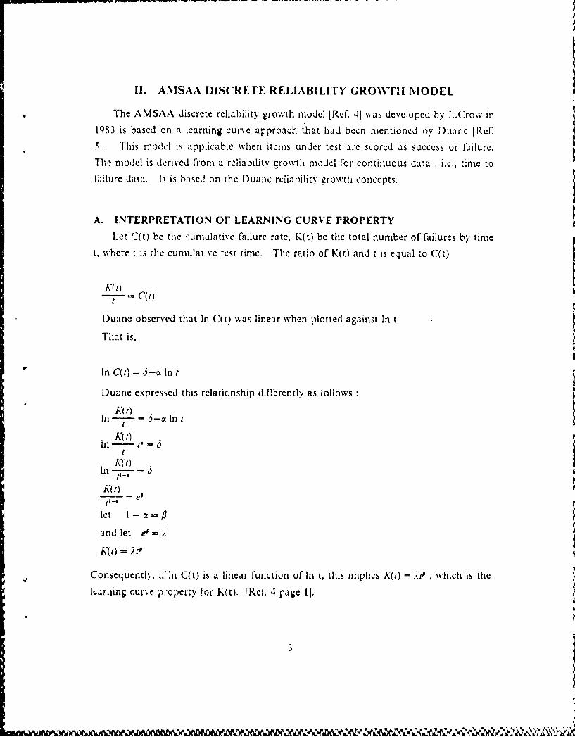
The AMSAA discrete reliability growth model f[Ref. 41 was developed by L.Crow in

19S3 is based on ri learning cure approach that had been mentioned by Duane [Ref.5]. This model is applicable when items under test arc scored as success or failure.The modcl is derived fromn a rcliability growth model for continuous data , i.e., time to

faIhilure data. It is based on the Duane reliability growth concepts.

A. INTERPRETATION OF LEARNING CURVE PROPERTYLet "'C(t) be the -numulative failure rate, K(t) be the total number of failures by time

t, where t is the cumulative test time. The ratio of K(t) and t is equal to C(t)

K( r)it

Duane observed that In C(t) was linear when plotted against In t

That is,

In C(t) = 5 -a In r

Duane expressed this relationship differently as followsKmt

In t = 6-a In t

t

K( t)

In -77- = -In - dKWt

= ei

let - a =f

and let e'=.

K(1) = ;..*

Consequently, iW"In C(t) is a linear function of In t, this implies K(t) =;t , which is the

learning curve property for K(t). [ Ref. 4 page 1I.

B. AMSAA DISCRETE RELIABILITY GROWTH MODEL DEVELOPMENT

The discrete reliability growth model developed at A.'VMSAAk uses attributes data.

This model is described as follows :

A = Number of trials for configuration i, i =1,2, ... ,k

T7 Cumulative number of trials through configuration i

T', - 'v,

T1= N, + -N2

In general :T, N \, + N,v + ,N, +.. + Nv,

Mt, = Number of failures for configuration i

K, Cumulative number of failures through configuration i

i K• = .At

K2 = Mt, - M,

In general:

K, = '1, + At2 + Mt + .+ 1,

E1A'] = Expected value of K,

The model assumes that log E[K,] is linear when plotted against log T,. This implies

E[KJ] = ., /,. [Ref. 4 page I to 4].

Elk,] = ).7T'= iN,&

PlT-

Ll K,] =? A= P,N,V + P2 N2

TY = -7

P2V = :71-PT

IV2In general:

P, N ,

[Ref. 4 page 5 to 6].

-l4

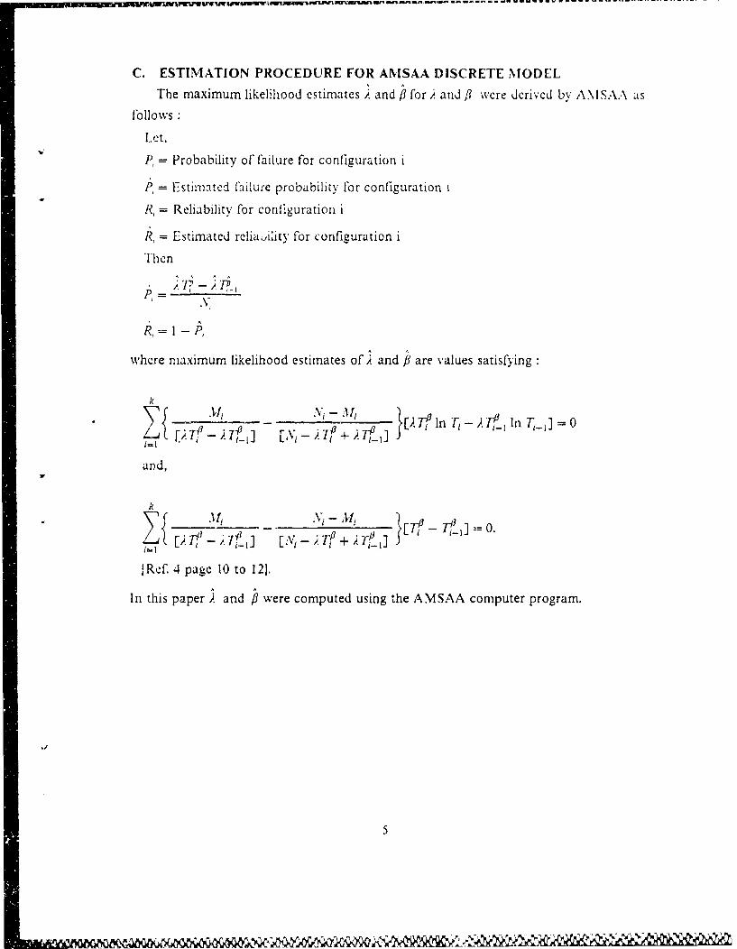
C. ESTIMATION PROCEDURE FOR ANISAA DISCRETE MODEL

The maximum likelihood estimates At and f for ,. and/f were derived by AISAA as

flbliows:

Let,

P, = Probability of 1'ailure for configuration i

I', = Estiniatd Failure probability for configuration i

R, = Reliability for configuration I

ý, = Estimated relia•,iity For configuration i

Then

where maximum likelihood estimates of ,A and fare values satisfying

k

V,_____ N. -1, rTip In Ti - I~ In T>]F). T - ).7-f [ 7e Al+A ] ;.7''jL0

and,

A

v. - i_•' TI"

+

P "?VIt~i - ;N- T" +T) -_]

[Ref. 4 page 10 to 12].

In this paper ). and ft were computed using the AMSAA computer program.

i5

III. EXPONENTIAL DISCRETE RELIABILITY GROWTH MODEL

The Exponential discrete reliability growth model has been analyzed at the Naval

Postgraduate School in two theses [Ref. 1, 21, and by Corcoran and Read [Ref 31, where

Corcoran and Read have compared several popular reliability growth models. This

model serves as a model comparison to the AMSAA discrete reliability growth model.

The Exponential discrete reliability growth model uses only attribute data. It does not

require any assumption about the distribution of the time to failure. This model is de-

scribed briefly as follows

Let :

R, = The reliability of the component in phase i

R,= I - expf - (o + fli)} where i =0, 1,2,..

i = 0 means the phase prior to any modification

The parameter estimates &, and /, of c and P for phase i are computed using linear

regression methods and an unbiased estimator for (o + fli)

F, =the total number of failure during phase i

V., =the number of tests between the 1)/- 1)f failure and je, failure, including the j"hin phase ij = 1, 2,3, ... , F,/

Yj. = unbiased estimator of", + fli) usingj-f sequence test in phase i

An unbiased estimator Y,, for (a + flu) [Chernoff and Woods 1965] is known to be:

i f ,•,, = I(+T + ... + if, +'-l Pv,_2

for i=0,1,2,... and j-= l, 2, 3, ... , .

Since N,.V , ,i .... F,,, are independent random variables, then

6

MaLIMMWUMMMI

., (r,,+ Y2., + ...- + -',,-

" is 'so ai unbiased estimates for (o + li)

"The least square estimates andfl, for a and /3 at phase i are

fill fo r i= 1, 2, 3,...

72j=O

and,

Y.,= -fl, i for i=1,2,3,...

where

T 11(Y,+ Y,+.+ 11)(i+ +)

: (0+ 1+2+."+/)(I+ 1)

By using &, and /3, the estimate of reliability for every phase i can be computed as fol-lowxs"

, I EXP( - (., + j,,)) for i= 1,2,3,...

The estimate of reliability for the original version of the component R() is given by

i&, = 1- EXP{- YFo} ,

[Ref. 6 page 3-i to 3-3].

In this paper the value of the mean regression estimate R, of reliability and the value

of standard deviation of the e-itimate of reliability S; were obtained from a computer

program used in J. Chandler thesis [Ref. 21. The equations for computing the reliability

growth values R, are easily solved using a hand-held calculator.

i7

IV. MONTE CARLO SIMULATIONS

Since the AMSAA model is interested in the number of trials until the r1 failureoccurs, the Monte Carlo simulation generates random variable using an algorithms de-veloped by Fishman 1978 [Ref. 71, and a subroutine from The New Naval PostgraduateSchool Random Number Package LLRANDOMIll 1981 [Rcf. 8] as a random numbergenerator for real uniform from 0 to 1. Given p , the probability of failure, and r, thenumber of failure for ever-y phase, the computer simulation generated the number oftrials until the e'A failure. Specifically let X be the random variable of interest, the num-ber of' trials until the r'h failure, then X is called negative binonmial random variable withparameter r and p. The probability function for X is,

Pj(k) = ( )pqk-r k=r,r+ l,r+ 2,.. r > 0

"The Algorithms for Computer Simulation

1. let A and B be double precision variables

2. w =(p),

3. Ifr•0, (I-p)<0, (I-p)>l, w•0, wŽ__l goto9

4. X=r, A=w, B=w and O=(l -p)(r.-1)

5. Generate U, uniform random number from 0 to I

6. If U: A or A >0.999999 or B <0.000001, go to 10

7. X=.X+I1, B=B(6IX+(l-p)) and A-=A+B

S. Go to 4

9. Print error message and stop

10. Continue.

[Ref. 7 page 354].

V. TEST PROCEDURE

The AMSAA model is evaluated using eight different sets of reliability values (the

actual growth pattern) and two different sets of inputs of number of failure per phase.

[his gives a total of sixteen cases. rable I describes all 16 cases. The set of reliabilityvalues for case i is the same as that for case i+ 8, i = 1, 2, ... 8. For cases I through

8 the number of failures per phase are equal to one and for cases 9 through 16 thenumber of failures per phase are equal to three. 'Ihe diagram in Figure 1 summarizes

the simulation procedure and the consequent analysis.

Table 1. ACTUAL RELIABILITY FOR 16 CASES

- CASE NUMBERS

"1,9 2,10 3,11 4,12 5,13 6,14 7,15 8,16

1 .600463 .408036 .899215 .408036 .408036 .408036 .404786 .400000

2 .600463 .408036 .899215 .804273 .804273 .691333 .598442 .43u000

3 .600463 .408036 .899215 .950990 .894416 .804273 .796763 .480000

4 .600463 .408036 .899215 .975249 .899963 .603542 .796763 .540000

5 .600-463 .408036 .899215 .990040 .899963 .600463 .802460 .610000

6 .600463 .408036 .899215 .990040 .899963 .755720 .802460 .700o)00

7 .600463 .408036 .899215 .990040 .899963 .849243 .857802 .800000

8 .600463 408036 .899215 .990040 .899963 .894416 .902960 .900000

9 .600463 .408036 .899215 .990040 .899963 .903636 .902960 .950000

10 .600-463 .408036 .899215 .990040 .899963 .903636 .902960 .990u00

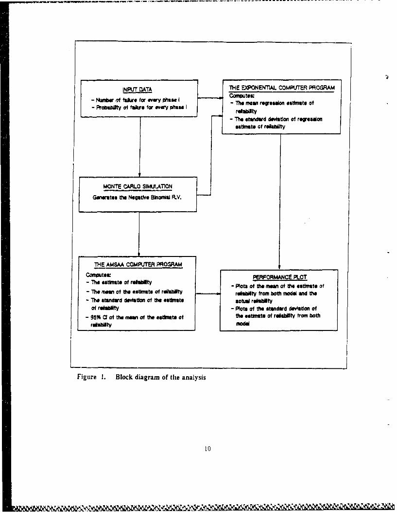
INPUT OATA THE EXXAEN'lAL COMPUTER PROGRAMComnwtses

- Numrdw of taJwu for every phase I - The moon regression estimate of- Pro~b•aty of fakr for f r every I ras

- The standard deviation of regrsedonestimate Gf reliabty

MONTE CARLO SIMULATTON

Generates the Negative Btonai R.V.

THE A•,wsA COMPUTER PROGRAM

Comnputes: PERFORMANCE LOT-The eatimlate of reOtlaty - Pots of t mo m of th state of

- The mem of ft estimate of raellAitY reiality from modal and fte- 7h standard deviation of the estimlltaie scW relhi~ty

of rellabty - Plots of the standard devIstion of

- 95% C of the meom of the estiate of the estamate of reaWb ltrom both

rebbilty model

L0Figure ~ ~ ~ ~ ~' 1. Blc igrmo h.aayi

V1. ANALYSIS PROCEDURE

v A. ACCURACY

Figures 4 through 35 in the .\ppendix provide a visual display of the AM SAA dis-

crete reliability growth model accuracy by compailrig tite growth line for the A, I SA.\

with the actual reliability growth pattern. These gramphs also provide plots For the [x-

ponential discrete reliability growth model using the same input data as that used in the

A\[ISAA discrete reliability growth model.

B. VARIABILITY

In addition to the tracking ability of the reliability point estimates R, , the user is

also interested in the variability o[fR,. Five hundred replications were run for each of

the 16 cases and each of the 10 phases, this provided

500

and,

500 -I- R1 )

Sý, = 499

for i= 1,2,.. ,10 for each of the 16 cases.

The algorithm used to compute the mean and standard deviation is developed by

Miller 1982 [Ref' 9 page 17 to 191. Standard deviation of the reliability estimates f'rom

both the AMSAA and the Exponential model are plotted.

11

C. CONFIDENCE INTERVAL

A 9 5 % two sided confidence interval for LI/,] is computed for each model for all16 cases. The equation used for these confidence limits are as follows

• (1.96)S k ,U, = R1 + -

and,

- (1.96)Si,Lj = R, - --

for i= 1, 2 ... , for each of the 16 cases.

12

VII. RESULTS AND CONCLUSIONS

The results for all 16 cases can be seen in the Appendix. The case number appears

at the table caption or at the figure caption. All of the results for each case are divided

into two categories, i.e., the tabulated statistic and performance plot. In this chapter

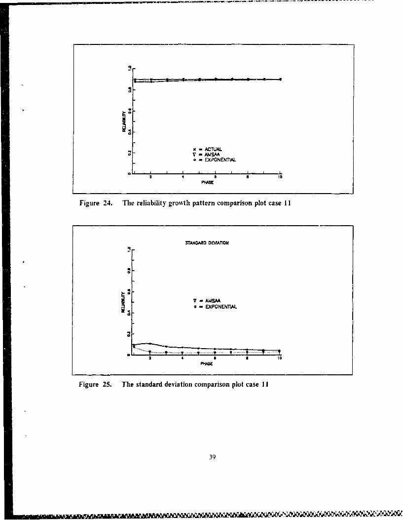
Table 2, Figure 2, and Figure 3 are explained as an example of the result fi-ora case I

of data set.

A. TABULATED STATISTICS

Table 2 indicates that testing was done until one failure occured after which a

change in the item was made. The actual reliability growth values for each of the 10

phases was constant at 0.60043, i.e., no growth actually occured. It is important to

simulate this case in order to examine the ability of the growth model to detect no

growth. Some reliability growth models have a built in assumption that.some grow-th

always takes place after a design change.

The values of R, For i = 1, 2, ... ,10 are given in colunu 4 for the AMSAA model

and in column 8 for the Exponential model, thus for phase 7, the AMSAA model yielded

R,=0.S0187 and the Exponential model yielded a value of 0.525144. The

coresponding values of the standard deviation are 0.124669 and 0.261854 for the

AMSAA and the Exponential model respectively.

B. PERFORMANCE PLOT

Figure I is a plct of R, versus i for the AMSAA and Exponential models. It also

displays a plot of the actual reliabilities R, . Figuie 2 is a plot of standard deviation for

case I for both the AMSAA and the Exponential model.

13

Table 2. STATISTICS FOR CASE I

OUTPUT of COMPUTER RUN> INPUT

-- DATAAMSAA MODEL EXPONENTIAL

MODEL

A--.n STD 95%b C1 of the STD> "vA- EAN MEANAC-- DEV of MEAN of'RLBT DEVTUAL Of the tileof of" T EST of EST of RGRS RGRSRLBT RLBT RLBT UPPER LOWER EST ES

EST JEST

1 1 .600463 .319489 .311700 .346811 .292167 .436848 .387013

2 1 .600463 .485770 .147713 .498718 .472823 .459899 .382840

3 1 .600463 .530347 .112104 .540173 520521 .482593 .316476

4 1 .600463 .553948 .103685 .563037 .544860 .515253 .292478

5 1 .600463 .569518 .106661 .578867 .560169 .509663 .282941

6 1 600463 .580187 .114242 .590201 .570173 .514700 .271440

1 .600463 .587260 .124669 .598187 .576332 .525144 .261854

8 1 .600463 .592922 .134212 .604686 .581158 .529729 .245836

9 .600463 .597331 .143335 .609895 .584767 .542551 .240164

10 1 .600463 .600715 .151730 j .614014 .58"7415 .550677 .219819

"14

1WUU~~1MMRkgK MNAMt.fJPU.IIJ'A

a-EXPONOETIAL

,_.4

0

!0

Figure 2. The reliability growth pattern comparison plot case 1

SrANDARD DEVIATION

,'F

0

V - AMSAA* - EXPONEN"TIAL

Figure 3. The standard deviation comparison plot case I

15

$1"AN .ARDA VA T C

= , . , .U wm.... - -,, '.'r nri njnr-yw rg . wn-., a-- , a n urn , n inc. a,-, a a, a . ',1-,, f.. ,',, ,, . .. .. . .. ,n ,. . .

C. SUMMARY AND CONCLUSIONS

To analyze the test results for cases I through H V all were divided into categories,

i.e., constant growth pattern, concave with rapid growth pattern, concave and convex

growth pattern, convex growth pattern (see Appendix).

1. Constant Growth Pattern

The AMSAA model didn't track the actual reliability too well for cases 1, 2, and

3 (the number of failure per phase was set equal to one). The AMSAA developed a

concave growth pattern, eventhough in these cases the actual reliability was constant.

Furthermore for case 3 the AMSAA model performance became worse since it had de-

creasing pattern and went below the actual reliability at phase 10. However when the

number of failure increased to three, the AMSAA model tracked the actual reliability

quite well. The mean of the estimate of reliability was close to the actual reliability, and

the standard deviation of the estimate of reliability was very small.

2. Concave itith Rapid Growth Pattern

This type of actual reliability growth pattern is represented in cases 4, 5, 12, and

13. The AMSAA model performed well in tracking actual reliability growth, especially

for case 4, case 5, and case 13, where it is close to the actual reliability with veiy small

standard deviation of the estimate of reliability. For case 12, the AMSAA model for

some reason could not track the actual reliability very well. It performed almost con-

stant growth, with a small decrease out through phase 10. This is a strange phenomena.

This case was run several times with the same result.

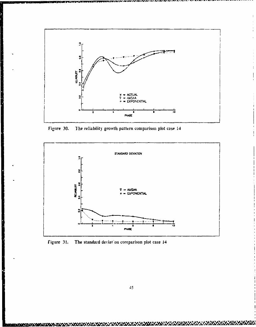
3. Concave and Convex Groisth Pattern

The AMSAA model has a problem tracking reliability growth pattern estab-

lished in cases 6, 7, 14, and 15. The AMSAA model seems to display a concave growth

pattern, it could not track the actual reliability which has a concave followed by a con-

vex growth pattern. This is probably because the cumulaxe assumption inherent in

the AM S..\A model does not work well when the reliability growth has a convex growth

pattern.

11

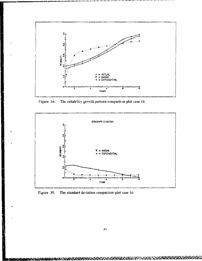
4. Convex Grosvth Pattern

The AMSAA model also had difficulty in tracking the actual reliability growth

pattern for cases 8 and 16, it ilust performed concave growth pattern fbr both cases.

The standard deviation of the estimate of reihabiiitv was good in these cases.

5. Summary

It appears that the ANISAA discrete reliability growth model is more appropri-

ate for reliability growth pattern that has the following characteristics

1. Concave with rapid growth pattern

2. Constant growth pattern with number of failure specified more than one.

It appears that the user should be wary of'using the AMSAA discrete reliability

growth model when the actual reliability growth has the following characteristics

1. Constant growth pattern with number of failures specified equal to one

2. Concave growth followed by convex growth pattern

3. Convex growth pattern.

Also the user should note that other discrete reliability growth models are available

which for some growth pattern performed better than the AMSAA model and which can

be programmed on a hand-held calculator.

17

aWT~lU W M D W t m tnuwnsnu I.R MRn EM. a M v ft.n ...u - - - . 1.--.

APPENDIX SIMULATION RESULTS: CASE 1 TO CASE 16

Table 3. STATISTICS FOR CASE I

OLVTPUT of COMPUTER RUNINPUTDATA

AMSAA MODEL EXPONENTIALA,,I O MODEL

"95% CI of the--> o MEAN STD MEAN of RLBT MEAN S' D

AC- DEV of I DEVTUAL of the the ofRLBT EST of E of RGRS RGRSRLBT RLBT UPPER LOWER EST EST

1 1 .600463 .319489 .311700 .346811 .292 167 .436848 .387013

2 1 .600463 .485770 .147713 .498718 .472823 .459899 .382840

3 1 .600463 .530347 .112104 .540173 .520521 .482593 .316476

4 1 .600463 .553948 .103685 .563037 .544860 .515253 .292478

5 1 .600463 .569518 .106661 .578867 .560169 .509663 .282941

6 1 .600463 .580187 114242 .590201 .570173 .514700 .271440

7 1 .600463 .587260 .124669 .598187 .576332 .525144 .261854

.600463 .592922 .134212 604686 .581158 .529729 .245836

9 1 .600463 .597331 .143335 .609895 .584767 .542551 .240164

10 1 .60046' 600715 .151730 .614014 .587415 .550677 .219819- - -

18

W�1"i..., - ,,,-...........

xACTUAL'" - A.MSAA

o- EXPONENTIAL

°1

Figure 4. The reliability gromth pattern comparison plot case I

STANDARD DEVIA710N

o - EXPONENTIAL

S...........g ............. • ........... ............. • ............ ... .. v .... .. . ... ..

.~~~ ~ -• | I | l .. L.2 4 10

Figure 5. The standard deviation comparison plot case I

19

Table 4. STATISTICS FOR CASE 2__________

OL IPL r of COMPUTER R.UNI PUT __ _ _ _ _ _ _ _ _ _ _ _ _

DA [

X'v[XA MDELMODEL

STD 95%' C I of theAC- MA DEV of MEAN of RLI3T M4EA N sm

TUAL o'te the of' oRLBT FST of EST of RG RS RGRS

_______ ______ UPPER A44 LOWER ES___ ESL

1 1 40386 41646 .6585 4841 .38274 .27941 .250027

3 1.006.451300 .110047 .422652 .403360 .342518 .2194326

7 1 4006 .394704 .128997 .406011 .383397 .340337 .252991

8 1 .403086 .376635 .157304 .3904214 .362847 .348798 .246473

9 1 .403086 .360838 .186914 .377221 .344454 .359013 .239996

10o 1 .403086 .346454 .215615 .365353 .3217554 .380852 .232067

20

.9i LyY'UAN 1W 11~ 1811&ý1G IL-.- IR D1

q

Sd

, x ,,ACTUALV AM4SM0 - EXPONENTIAL

S I II I ,..

2 4 O S 10


STANnARD DEVIATION

Jq

J0

V - AAISAA• - EXPONENT1AL

4 i

Figure 7. The standard deviation comparison plot case 2

21

-i

Table 5. STATISTICS FOR CASE 3

OUTPUT of COMPUTER RUN

,-. INPUTDATA

EXPONENTIALAMSAA MODEL MODEL

SSTD 95% CI of the

- AC- MEAN DEVof MEAN of RIBT MEAN DEVTUAL of the the ofof ofTUAL EST of EST ofRGRS RGRS

RLBT RLBT UPPER LOWER EST EST

I 1 .899215 .397305 .339065 .427025 .367585 .784433 .293429

2 1 .899215 .764665 .098591 .773307 .756023 .797078 .288337

3 1 .899215 .839154 .060455 .844453 .833855 .822922 .225154

4 1 .899215 .868815 .046403 .S72882 .864747 .837676 .186795

5 1 .899215 .885368 .041623 .889016 .881719 .834702 .192540)

6 1 .899215 .896082 .039685 .899561 .892603 .852273 .159859

7 1 .899215 .903360 .039227 .906798 .899921 .85S921 .134S09

8 1 .899215 .908869 .039064 .913293 .905444 .869732 .120620

9 1 .899215 .913205 .038957 .916620 .909790 .870845 .119773

10 1 .899215 .916762 .038813 .920164 ,913360 -.876847 .109467

22

............................................................................................

o -ACTUAL

0-EXPONMMiAL

[ 4. lAS to

Figure 9. The reliability groith pattern comparison plot case 3

STANDARD DE'VIATION

0

V - AAASM

-EXPONENTIAL


23

,,,,,, . . .•, ,• ., •, i•• • •-• • • 'ln .",•"•l • r• • • •


> OUTPUT of COMPIUTER RUN

INPUT ....DATA

EXPONENTIALAMSAA MODEL MODEL.

STD 95% CI of the SIDMEAN MEAN of RLBT MEAN DAC- of the DEV ofof

TUAL EST of" the RGRS 0rRRB LT EST of ST RG RSRLB' RLBF RLBT UPPER LOWER EST [ST

1 1 .403086 .247188 .301170 .273586 .220789 .277941 .350039

2 .,804723 .831764 .062844 .837272 .826255 .692599 .334232

3 1 .950990 .923927 .033311 .926847 .921007 .900547 .166031

4 1 .975249 .960687 .019283 .962377 .958997 .960575 .075075

5 1 .990040 .978110 .013216 979269 .976952 .985843 .022317

6 1 .990040 .985506 .011104 .986480 .984533 .993530 .022859

7 1 .990040 .988832 .009410 .989657 .988007 .993346 .011663

8 1 .990040 .990717 .009306 .991532 .991066 .994365 .010904

9 1 .990040 .991889 .009384 .992711 .991066 .994678 .009990

10 1 .990040 .992741 .008820 .993514 .991968 .994922 .009867

24

x - ACTUALV - AMSMo - EXPONENTIAL

I 5 I


TTANIWR DCVIA71ON

* - EXPONENTIAL

2 4 U I0


25



INPUTDATA- EXPONENTIAL

AMSAA MODEL MODEL

4t. STD 95% C l of the

MEAN MEAN of RLBT MEAN STDAC- of the ____of of" DEVTUAL EST of the ofRLBT EST of RGRS RGRSRLB' RLBT UPPER LOWER [ST EST

1 1 .4030S6 .304970 .319788 .333001 .276939 .277941 .353039

2 I .804723 .716657 .099573 .725385 .707929 ,692599 .334232

3 1 .894416 .811904 .063882 .817504 .806305 .816604 .229131

4 1 .899963 .854719 .050648 .859159 .850280 .857286 .180176

5 1 .899963 .877544 .045115 .881498 .873589 854340 .201203

6 1 .899963 .891553 .042322 .895262 .887843 .852018 .233083

7 1 .899963 .900743 .041174 .904352 .897134 .883001 .196564

8 1 .899963 .907577 .040321 .911111 .904042 .880019 .208935

9 1 .899963 .912850 .039735 .916332 .909367 .886436 o½9224

10 1 .899963 .917156 .038932 .920568 .9(3743 .889895 .215450

26

in awini .ir.,.inasnasi i,.I m~lalat-.ail ian iraa. n ni -..l~flI • . -- - .- ---

IR

S• ACTUAL

o - EXPONENTIAL

24 I I4


STAN DARo DEvmTnON

I: V - AMSMAo - EXPONENTIAL

""1.

". . ......... ............. ..........S 1 • I p I , , ..

2 4 S I IC


27


P OUTPUT of COMPUTER RUN7:-:. IN PUT

DATAEXPONENTIAL

AMSAA MODEL MODEL

S-D 95% CI of the-- MCEAN "MEAN of RLBT MEAN Dr"• AC- of the DEV of of' DEV

TUAL EST of the at ofRLBT EST of EST of RGRS RGRS

RLBT UPPER LOWER EST EST

1 1 .403086 .224899 .271434 .248692 .201,107 .277941 .350039

2 1 .691333 .630239 .101236 .639112 ,621365 .566627 ,371685

3 1 .804723 .728316 .078056 .735158 .72147,4 .702538 .282617

4 1 .603542 .768103 .070584 .774289 .761916 .649254 .242711

5 1 .600463 .787819 .064749 .793495 .782144 .609683 .240854

6 1 .755710 .805681 .061914 .811108 .800254 .674674 .217185

7 1 849243 .823900 .062269 .829358 .818442 .763961 .167637

8 1 .894416 .841536 .063679 .847117 .835954 .830485 .122824

9 1 .903636 .855559 .064934 .861250 .849867 .865976 .105627

10 1 .903636 .866080 .064945 .871772 .860387 .889152 .084728

28

qu

X-ACTUALV - AMSUMo- EXPONENTIAL

2 4 B I 10


STANDARD •EVIATION

V - A)JSA• -,XPONUMTIAL

I I I I _. t I -


29



SINPUTDATA

EXPONENTIALAMSAA MODEL MODEL

It: 95% CI of the-o MEAN T MEAN of RLBT MEAN STD

AC- of tile DEV of of DEVTUAL EST of' the RGRS ofRLBT EST of EST RGRS

RLBT RLBT UPPER LOWER EST

1 1 .404786 .304970 .319788 .333001 .276939 .262647 .346369

2 1 .598442 .716657 .099573 .725385 .707929 .474285 .378478

3 1 .796763 .811904 .063882 .817504 .806305 .678456 .301077

4 1 .796763 .854719 .050648 .859159 .8502S0 .747581 .244811

5 1 .802460 .877544 .045115 .881498 .873589 .752545 .242109

6 1 .802460 .891553 .042322 .895262 .887843 .764293 .257599

7 1 .S57S02 .900743 .041174 .904352 .897134 S816030 .237079

8 1 .902960 .907577 .040321 .911111 .904042 .842211 .241987

9 1 .902960 .912850 .039735 .916332 .909367 .853594 .251411

10 1 .902960 .917156 j038932 .920568 .913743 .855511 .253041

3 0

... • ........ .. 9 .... ....... ..... •

x.ACTUALV - AMSAAo - EXPONENTIAL

2 41 10

Figure 16. The reliability gro~ith pattern comparison plot case 7

SYMAR Dg D I eMTION

-AJJSAA

0-EXPONENTIAL

'"V......,...g ~ ~ ~........... 9 .... .l ............ ............ ....... p ............ ...... 4

3 4 S I 10


31

NRUU



INPUTDATA EXPONENTIAL

AMSAA MODEL MODEL

-TD 95% CI of the STDSMEAN STD MEAN of RLBT MEAN ADNTAC- of the DEV of of DEVTUAL EST of tile RG RS o f

RLBT RLBT EST of RS RGRSRLBIT UPPER LOWER EST EST

S 1 .400000 .149057 .192978 .16<972 .132142 .271768 .344556

2 1 .430000 .687404 .080545 .694464 .680344 .305861 .350305

3 1 .480000 .769958 .064798 .775638 .764279 .389910 .3217S3

4 1 .540000 .812713 .056419 .817658 .807767 .449303 .284744

5 1 .610000 .841962 .051100 .8' :u441 .837483 .561109 .261834

6 1 .700000 .864439 .047810 .868630 ,86024'; .621144 .238394

7 1 .800000 .883575 .045648 .887577 .879575 .712991 .196329

8 1 .900000 .903105 .043961 .906959 .899252 .816562 .138561

9 1 .950000 .922076 .042662 .925816 .918337 .894838 O0S7652

10 1 .990000 .945008 .042874 .948766 .941250 .959923 .034246

32

q

p/ x .ACTUAL

o• o - F.XPONENTLAL

{ l, I I I , I I I I I

2 4 5 t

Figure 18. The reliability growlth pattern comparison plot case 8

STANDARD DEVMAllON

V - ANISMo - EXPONENTIAL

2 4 5 S 10


33



INPUT _______________ _____

DA).TAEXPONENTIAL

AMS.XA MODEl. MODEL

<.,-'m 951,,"o CI or"the"- MEAN of RI..BT STEAN S)

* AC- OF the DEV of' of DEVTUAL EST ofe the of'R, T RL [B EST of S RRs

RLBT UPPER LOWER [ST EST

1 3 .600463 .538802 .186346 .555136 .522168 .553655 .210395

2 3 .600463 .576379 .086393 .583952 .568807 .563631 .218474

3 3 .600463 .585S66 .063621 .591443 .5S0289 .560046 .196348

4 3 .600463 .590186 .057592 .595234 .585138 .571343 .179061

5 3 ,600463 .592796 .058542 .597928 .587665 .583947 .15,4435

6 3 .600463 .594467 .062527 .599947 .588986 .586601 .147665

7 3 .600463 .595507 .067578 .601431 .589584 .587442 .140020

8 3 .600463 .596269 .072753 .602646 .589891 .586170 .137124

9 3 .600463 .596791 .077717 .603603 .589979 .592676 .123858

10 3 .600463 .596975 .082442 .604201 .589749 .589863 [ .116577

34

-r

AMA

V - AMCTAL

0- EXPONENTIAL

I ,0 I I I I I ,,

2 4 |I


STANDARD DEVIATION

I0 V A.MiSMo - EXPONENTIAL

. ............ . ....... ..... ..... ...... ............

2 4 S 3 10

Figure 2i. The standard deviation comparison plot case 9

35



INPUTDArA

AMSAA MODEL EXPONENTIALMODEL

SM95% CI of the-MEAN ST)D MEAN of RLBT MEAN SED," AC- of' the DEV of of DEV

TUAL EST of the RGRS ofRLBT RLBET EST of RS RGRS

RLBT UPPER LOWER [ST EST

1 3 .403086 .365701 .228152 .385700 .345703 .348426 .225386

2 3 .403086 .398549 .130351 .409974 .387123 .375728 .235090

3 3 .403086 .404570 .096573 .413035 .396105 .378259 .202326

4 3 .403086 .405363 .077487 .412155 .398571 .391223 .180188

5 3 .403086 .404514 .068972 .410559 .398468 .400876 .173112

6 3 .403086 .402537 .070057 .408678 .396397 .403065 165447

7 3 .403086 .399935 .078909 .406851 .393018 .399075 .157684

8 3 .403086 .397170 .091792 .405216 .389124 .393748 .154780

9 3 .403086 .394409 .106329 .403729 .385089 .400769 .139954

10 3 .403086 .391858 .119968 .402374 .381342 .396243 .130672

36

VL -- MS

o - EXPONENTIAL

CL2 4 S I 10

PHMJ


STANDARD DMATION

V - A)JSMo - EXPONENTIAL

" ........ .. . . .S. . .... ..... ..... ....... .... . .. .....V ...... . .I .. . ..

2 4 S I Ia


37


K OUTPUT of COMPUTER RUN

7! INPUTD.A\TA D EXPONENTIAL

AMSAA MODEL.MDF MODEL

950 CI of theTA MEAN SID MEAN of RLBT MEAN STE)SAC- of' te DEV of of DEV

T'AL EST of the RGRS ofRLBT .LBT f ESr of" RGRS

RLBT UPPER LOWER EST EST

1 3 8S99215 .874708 .075400 .S81317 .868099 .875154 .097891

2 3 .899215 .890215 .030085 .892852 .887578 .874634 .108637

3 3 .899215 .893745 .022208 .895692 .891798 .881110 .080530

4 3 .899215 .895290 .019809 .897027 .893554 .885150 .071685

5 3 899215 .896174 .019993 .897927 .894422 .887219 .062968

6 3 .899215 .896677 .021320 .898545 .894808 .889853 .058065

7 3 .899215 .896921 .022891 .898928 .894915 .890704 .054956

8 3 .899215 .897091 .024281 .899219 .894962 .890799 .051037

9 3 .899215 .897191 .026041 .899473 .894908 .893297 .045739

10 3 .899215 .897171 .027662 .899596 .894747 .892541 043866

38

-a.,. - .

---

.q

.z - I l , I i - H

SSbx = ACTUALV - MSM

-EXPONENTIAL

012 10


STANDARD DEVIATION

E XP•ONENTIAL

2 4 0 a t]


39

Table 14. STATISTICS FOR CASF 12


71 INPUTDATA

AMSAA2 MODEL EXPONENTIALMODEL

M N SD 95% CI of the STD- MEAN SDE MEAN of RLBT M'lEAN .DLAC- of the DEV of of oDVTUAL EST of tile RG RS of

RLBI RLBT EST of ES RGRSRLBT UPPER LOWER [ST EST

1 3 403086 .841201 .098829 .849864 .832538 .348426 .225386

2 3 .804723 .849013 .046282 .853069 .844956 .771284 .162229

3 3 .950990 .841209 .050197 .845609 .836809 .939463 .044327

4 3 .975249 .833962 .078297 .840825 .827099 .976039 .017360

5 3 .990040 .830465 .090770 .838422 ý822509 .990117 .010184

6 3 .990040 .829695 .091803 .837830 .821561 .993581 .009200

7 3 .990040 .828934 .094342 .837247 .820620 .994806 .008335

8 3 .990040 .828181 .096894 .836674 .819688 .995307 .008680

9 3 .990040 .827444 .098868 .836110 .818778 .995613 .008335

10 3 .990040 .826714 100896 .835558 .817870 .995641 .008335

40

...........a a. ' ' . ...... ..... ...... .. .... ....... ..........

x - ACTUAL

V - NASMA- EXPONENTIAL

2 4. 5 5

PKASE


STANWARU DEmXFnON

V - AMSMo - EXPONENTIAL


41



INPUTDAASAAMODEL

EXPONENTIALAMSAAMODELMODEL

STD 95% C1 of the STD- AC- MEAN DEVof MEAN of RLBT MEAN DEVTUAL of the tie of of

RLBT ESI of RGRS RGRSRLBT RLBT UPPER LOWER. ESET

1 3 .403086 .421329 .242162 .442556 .400103 .348426 .225386

2 3 .804723 .751290 .060248 .756570 .746009 .771284 .162229

3 3 .894416 .833149 .034031 .836132 .830166 .887470 .074325

4 3 .899963 .868939 .026237 .871239 .866639 .913950 .052619

5 3 .899963 .887645 .023565 .889711 .885580 .921667 .042965

6 3 .899963 .899931 .022328 901348 .897433 .924828 .039463

7 3 .899963 .907487 .021942 .909410 .905564 .925187 .037596

8 3 .899963 .913555 .021536 .915443 .911667 .924395 .035405

9 3 .899963 .918287 .021365 .920160 .916414 .925071 .031639

10 3 .899963 .922147 .021066 .923994 .920301 .923207 .031085

42

S... .. ...."..

x - ACTUAL9= -MSAAo= EXPONENTIAL

-- I I I ID


STANDARD DEW'IAT1ONq

V - AMSAAo - EXPONENTIAL

S........... . . . . . . .- . . . . . - ; - ; - .. . . . . -2 4 S 6l ID


43

**!-P tVWX l 4~NAP NIN. V ~ ~ N~~~~1



INPUTDATA

EXPONE.,TIAALzAMSAA MODEL MODEL

STS 95% CI ofr the-- AC- vEAN SDV MEAN of RLBIF MEAN DTV,- AC- of' thes DEV of MEof' DEV

TUAL EST ofe the RG OfRL13T EST of RGRS

RLBT RLBT UPPER LOWER EST EST

1 3 .403086 ,299748 .196088 .316936 .282561 .348426 .225386

2 3 .691333 .659017 .062098 .664460 .653574 .655112 .193326

3 3 .S04723 .750623 .043777 .754460 .746785 .788019 .117403

4 3 .603542 .787263 .038458 .790634 .783892 .713682 .126110

5 3 .600463 .803674 .034742 .806720 .800629 .671260 .120385

6 3 .755710 .819347 .032614 .822205 .816488 .720426 .110446

7 3 .849243 .836709 .032380 .S39548 .833871 .794972 .084335

8 3 .894416 .853894 .032927 .856780 .851008 .851854 .063108

9 3 .903636 .867828 .033429 .870758 .864897 .S86990 .044668

10 3 .903636 .878133 .033186 .881042 .875224 .903086 .038209

44

X .ACTUAL

- E• XPONENTA

0 1 I I I I 1

Figure 30. ihe reliability grovtli pattern comparison plot case 14

S1ANUARD DEVIAT1ON0

V1 - AMSAAo - EX0ONENTIAL

Y. * . II t

Figure 31. The standard devial'on comparison plot case 14

45

rflW -- -- - ... - .. .. . -�

Tab1e� 17. STATISTICS FOR CASE 15

*


INPUT _______________________________ _______________

1)AT�\EXPON [ENTIA L

AMSAA MODEL. MODEL

��1

MEAN STD 95% CI of the STI)AC- of th� DLV of MEAN of RL1IT MEAN DLV

______ of'TUAL EST of the RGRS ofRL.BT EST of RGRS

RLBT RLBT UPPER LOWER EST [ST

1 3 .404786 .421329 .242162 .442556 .400103 .351763 .225708

2 3 ,59844) .751290 .060248 .756570 .746009 .561042 .2 19583

3 3 .796763 .833149 .034031 .836132 .830166 .761750 .128729

4 3 .796163 .86S939 .026237 .871239 .866639 .807520 .102913

5 3 .S02460 .887645 .023565 .889711 .885580 .828525 .080055

6 3 .802460 .899391 .022328 .901348 .897433 .836119 .073760

7 3 .857802 .907487 .021942 .909410 .905564 .860585 .061728

8 3 .902960 .913555 .021536 .915443 .911667 .890172 .048793

9 3 902960 .918287 .021365 .920160 .916414 .907881 .037583

10 3 1902960 .922147 .021066 .923994 .920301 .915806 .033604-I- t. I _____________ I _____________ ______________ ____________ _____________

46

= EXPONENTIAL

2 4Sa 10

Figure 32. The reliability grwstli pattern comparison plot case 15

STANDARD DEVIATION

V = AMSMAa- EXPONENTIAL

....... ..".. .... '*2 0 10I

_ _ PHASE

Figure 33. The standard deviation comparison plot case~ 1 5

47V


OUTPUT of COMPUTi'R RUNSINPIUT _ _ _ _ _ _ _ _ _ _ _ _ _ _ _ _ _ _ _

DATAEXPONE NTIAL

AMSAA MODEL L MODEL

i5; :v,:95°,,, CI of"the1 MEAN SD' SAN f )

AC- lie DEV of 1)A f BV

TUAL J.S of the RGCRS ofRLB[ R ES-1 of EST RGRS

RLBT LUPPER LOWER ESIr

1 3 .400000 .228712 .160711 .242799 .214625 .344437 .225569

2 3 .430000 .594215 .066121 .600011 .588419 .400345 .238088

3 3 .480000 .6772.784 .053963 .677514 .668054 .444004 .202921

4 3 .540000 .716845 .049957 .721224 .712466 .506867 .180221

5 3 .610000 .748614 .048I21 .752832 .744396 .578905 .150044

6 3 .700000 .774650 .047420 .778807 .770494 .659072 .127605

7 3 .800000 .798445 .047698 .802626 .794264 .746996 .099554

8 3 .900000 .824266 .048878 .828550 .819981 .839623 .066243

9 3 .950000 .851483 .050970 .855951 .847016 .909948 .036966

10 3 .990000 1.863599 .051552 [868118 .859080 .964 63 .016538

48

g llfiiiiii

16-t

y -, ACTUALo - y EXPONENTIAL

o LL.. • ... ,.....• I I | ,....I ..

4

F~igure 34. The reliab~ility gro~th pattern comparis'in plot case 16

SV m AMAA

o -, EXPONENTIAL

S. .......... ............ ... ......... ........... . .. . . . . . • . . . - . • : , . . ..I10


49

LIST OF REFERENCES

1. Drake, J. E., Discrete Reliability Growth Miodel Using Failure Discounting, Naval

Postgraduate School, Montercy, California, September 19S7.

2. Chandler, J., Estimnating Reliability with Discrete Growth Models, Naval Post-

graduate School. Monterev, California. March 1988.

3. Corcoran, W. J., and Read, R. R., Comparison of Some Reliability Growth !sti-

mation and Prediction Schernes, United Technology Center Report, Addendum.

VTC 2140, 1967.

4. Crow, L. [I., AMISAA Discrete Reliability Growth Model, US Army Material Sys-

tem Analysis Activity, Aberdeen Proving Ground. Maryland, 1983.

5. Duane J. T., Learning Curve Approach to Reliability Monitoring, IEEE Trans-

action On Aerospace, volume 2 number 2, April 1964.

6. Woods, W. M., Reliability Growth Model, paper presented at a meeting of the

Avionics Panel held in Ankara, Turkey, 9-13 April 1979.

7. Fishman, G. S., Principle of Discrete Event Simulation, Wiley Series on System

Engineering and Analysis, 1978.

8. Lewis, P. A., and Uribe. L., the New Naval Postgraduate School Random Number

Package LLIRA-NDOMII, Naval Postgraduate School, Monterey, California, 1981.

9. Miller, A. R., FORTRAN Programs for Scientist and Engineers, Sybex Inc, 1982.

50

IN~IA IISTRILIU [ION LIST

D)ekcw~c T echinical Tnfoilriatioll 'Cll~tcI

C.výImcrotlStgriitechoNiocerx.VA 22304-614.o

3. Deja rtrn Cod 01-1)an(i~e~

Navilostiaduthtc schooloNtCIce,- cv A 939-43-5f

4. Dp~lrotsriw t MCh J ) Ods. od 5 WDeparFtment of Operarioii Research

Naal[osunraduatt School)Muloterev, CA 93943,

5. roFeCSsýor Roer R.'I Weadý. C"ode 55 ReDeparinent ucnofOperaticons Research,Nzt'~al Postrgradualte SchIoolM onterev, L.\ 93943

5. Pcro.eso Riobia t R. Read', Code 515 ReDepartmntci oF O.perations Research

Na'.a OstLcrdLaatC SchoolMontreyCA 93943

17. P~er[Pn';takXaan Akadenil TNI-ALPuiackalan L dara Adisu~tjiptoJogjakartaINDON\ESIA-

S. \f ax or ( Pnb) Rio M. Thalier)DiirCktorat Pendidikan Niabes TN 1WUAi. Gatot SubrotoJaikarta1 NDONIZSIA

5'

naval postgraduate school monterey, californ a file •,u, · naval postgraduate school monterey,...

Documents