ndhms v4.3 tech note user guide v1.0
TRANSCRIPT
DRAFT
The NCAR Distributed Hydrological Modeling System (NDHMS)
User‟s Guide and Technical Description
Version 4.3
Created:
March 10, 2010
David J. Gochis
Wei Yu
David N. Yates
DRAFT
Table of Contents
ACKNOWLEDGEMENTS
Introduction:
Brief History
Model requirements
Model Physics Description:
Overview
Land model description
Terrain routing descriptions
Channel and lake routing description
Baseflow/Groundwater model description
Model Technical Description and User Guide:
Description of code
Setup and execution of uncoupled NDHMS code
Comment on Cold start (arbitrary initial conditions vs.
RESTART)
Setup and execution of coupled WRF-NDHMS code
NDHMS Input and Output Data structures:
Domain processing
Description of input files
Description of output files
Description of parameter files
Description of namelist file
APPENDICES:
NDHMS model namelist description
Vegetation parameter table (VEGPARM.TBL)
Soil parameter table (SOILPARM.TBL)
General parameters table (GENPARM.TBL)
Channel parameters table (CHANPARM.TBL)
Lake parameters table (LAKEPARM.TBL)
Groundwater/baseflow bucket model parameters table
(GWBUCKPARM.TBL)
Forcing data netcdf file header
Land model output netcdf file header
High-resolution terrain model netcdf file header
Channel observation point netcdf file header
Channel network point netcdf file header
Lake point netcdf file header
Land fluxes ASCII output file (lnd_fluxes.txt)
Channel inflow ASCII output file (chan_inflow.txt)
Forecast/observation point ASCII output file (frxst_pts.txt)
Groundwater inflow ASCII output file (GW_inflow.txt)
Groundwater outflow ASCII output file (GW_outflow.txt)
Groundwater level ASCII output file (GW_zlevtxt)
Listing of model constants (e.g. specific heats, latent heat terms, w/
units (not yet developed)

ACKNOWLEDGEMENTS
The development of the NCAR Distributed Hydrological Modeling System (NDHMS)
has been significantly enhanced through numerous collaborations. The following persons
are graciously thanked for their contributions to this effort:
Fei Chen, National Center for Atmospheric Research
John McHenry and Carlie Coats of Baron Advanced Meteorological Services
Zong-Liang Yang, Cedric David and David Maidment of the University of Texas at
Austin
Harald Kuntsmann and Benjamin Firsch of Karlsruhe Institute of Technology
Ismail Yucel (XXX Turkey)
Blaine XXXX (U.S. Bureau of Reclamation)
Funding support for the development and application of the NDHMS has been provided
by:
The National Science Foundation and the National Center for Atmospheric Research
Baron Advanced Meteorological Services
National Aeronautics and Space Administration (NASA)
National Oceanic and Atmospheric Administration (NOAA) Office of Hydrological
Development (OHD)

Introduction The purpose of this technical note is to describe the physical parameterizations,
numerical implementation, coding conventions and software architecture for the NCAR
Distributed Hydrological Modeling System (NDHMS). Chapters 1-4 provide the
historical development of the NDHMS along with descriptions of the currently
configured land surface model (Chapter 2), terrain routing algorithms (Chapter 3),
channel and reservoir routing algorithms (Chapter 4) and a simple, empirical baseflow
algorithm (Chapter 5). Chapters 6-10 provide detailed descriptions of the input and
output datasets, procedures for pre-processing model input fields required for routing
operations and model parameter and namelist datafiles. Coding conventions, steps for
model implementation in both uncoupled NDHMS and coupled WRF-NDHMS are
provided in Chapters 11-13 respectively. Lastly, examples and descriptions of all major
input, output, parameter and namelist files are provided in the Appendices.
Brief History
The NCAR Distributed Hydrological Modeling System is a fully distributed, 3-
dimensional, variably-saturated flow model built upon a modularized FORTRAN90
software architecture. Initially, the implementation of terrain routing and, subsequently,
channel and reservoir routing functions into the 1-dimensional Noah land surface model
was motivated by the need to account for increased complexity in land surface states and
fluxes and to provide physically-consistent land surface flux and stream channel
discharge information for hydrometeorological applications. The original
implementation of the surface overland flow and subsurface saturated flow modules into
the Noah land surface model were described by Gochis and Chen (2003). In that work, a
simple subgrid disaggregation-aggregation procedure was employed as a means of
mapping land surface hydrological conditions from a „coarsely‟ resolved land surface
model grid to a much more finely resolved terrain routing grid capable of adequately
resolving the dominant local landscape gradient features responsible for gravitational
redistribution of terrestrial moisture. Since then numerous improvements to the Noah-
distributed model have occurred including optional selection for 2-dimensional (in x and
y) or 1-dimensional („steepest descent‟ or so-called „D8‟ methodologies) terrain routing,
a 1-dimensional, grid-based routing model, a reservoir routing model, and a simple
empirical baseflow estimation routine. Furthermore the entire new modeling system,
now referred to as the NCAR Distributed Hydrological Modeling System (NDHMS) has
recently been coupled to the Weather Research and Forecasting (WRF) mesoscale
meteorological model (Skamarock et al., 2005) thereby permitting a physics-based, fully
coupled land surface hydrology-regional atmospheric modeling capability for use in
hydrometeorological and hydroclimatological research and applications. Lastly, the code
has been fully parallelized for high-performance computing applications.
Model Requirements
The 3-dimensional, NDHMS has been developed to represent the spatial redistribution of
overland flow and shallow saturated subsurface soil moisture. Switch-activated modules
enable treatments of terrestrial hydrological physics (see Figure 2), which have etiher
been created or have been adapted from existing distributed hydrological models.
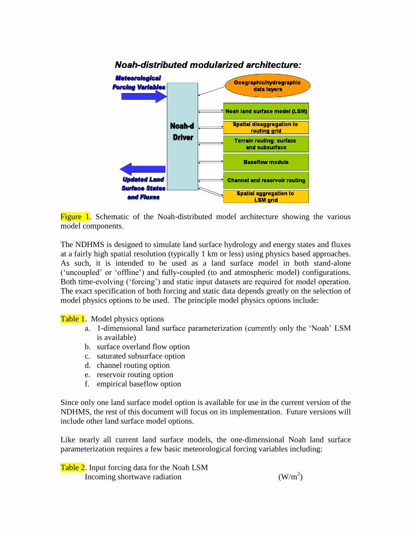
Figure 1. Schematic of the Noah-distributed model architecture showing the various
model components.
The NDHMS is designed to simulate land surface hydrology and energy states and fluxes
at a fairly high spatial resolution (typically 1 km or less) using physics based approaches.
As such, it is intended to be used as a land surface model in both stand-alone
(„uncoupled‟ or „offline‟) and fully-coupled (to and atmospheric model) configurations.
Both time-evolving („forcing‟) and static input datasets are required for model operation.
The exact specification of both forcing and static data depends greatly on the selection of
model physics options to be used. The principle model physics options include:
Table 1. Model physics options
a. 1-dimensional land surface parameterization (currently only the „Noah‟ LSM
is available)
b. surface overland flow option
c. saturated subsurface option
d. channel routing option
e. reservoir routing option
f. empirical baseflow option
Since only one land surface model option is available for use in the current version of the
NDHMS, the rest of this document will focus on its implementation. Future versions will
include other land surface model options.
Like nearly all current land surface models, the one-dimensional Noah land surface
parameterization requires a few basic meteorological forcing variables including:
Table 2. Input forcing data for the Noah LSM
Incoming shortwave radiation (W/m2)
Incoming longwave radiation (W/m2)
Specific humidity (kg/kg)
Air temperature (K)
Surface pressure (Pa)
Near surface wind in the u- and v-components (m/s)
Liquid water precipitation rate (mm/s)
[Different land surface models may require other or additional forcing variables or the
specification of forcing variables in different units.]
When coupled to the WRF regional atmospheric model the forcing data is provided by
the atmospheric model with a frequency dictated by the land surface model time-step
specified in WRF. When run in a stand-alone mode, these forcing data must be provided
as gridded input time series. External, third party, Geographic Information System (GIS)
tools are used to delineate a stream channel network, open water (i.e., lake, reservoir, and
ocean) grid cells and baseflow basins. Water features are mapped onto the high-
resolution terrain-routing grid and post-hoc consistency checks are performed to ensure
consistency between the coarse resolution Noah land model grid and the fine resolution
terrain and channel routing grid. Further details on the preparation of forcing data for
stand-alone NDHMS execution is provided in Chapter XX.
The NDHMS calculates fluxes of energy and moisture either back to the atmosphere or as
stream and river channel fluxes. Depending on the physics options selected, the primary
output variables include:
Table 3. Output data from the NDHMS:
Surface latent heat flux
Surface sensible heat flux
Ground surface and/or canopy skin temperature
Surface evaporation components (soil evaporation, transpiration, canopy water
evaporation, snow sublimation and ponded water evaporation)
Soil moisture
Soil temperature
Deep soil drainage
Surface runoff
Canopy moisture content
Snow depth
Snow liquid water equivalent
Stream channel inflow (optional with terrain routing)
Channel flow rate (optional with channel routing)
Channel flow depth (optional with channel routing)
Reservoir height (optional with channel routing)
The NDHMS utilizes a combination of netcdf and flat ASCII file formats for input and
output and therefore requires that netcdf libraries be installed on the local machine
executing the simulations. For information regarding netcdf data structures and where to
obtain netcdf libraries please visit the official netcdf website hosted by UNIDATA at:
Computational/Hardware Requirements
The NDHMS has been developed on a LINUX-based computing platform using Portland
Group FORTRAN90 compilers. To date the only other platform the model has been
ported to is the IBM supercomputer „bluefire‟ located at NCAR and not been rigorously
tested on other platforms. When run in full hydrologic simulation mode, with all
attendant process modules activated (e.g. overland and subsurface routing, channel and
reservoir routing, and baseflow) the NDHMS is a moderately computationally-intensive
modeling system with respect to other physics-based environmental modeling systems
(e.g. weather models climate models, catchment hydrology models and other geophysical
fluid dynamics models). However, computational requirements scale exponentially as
functions of domain size and spatial resolution. Thus there are no firm rules on minimum
computational requirements in terms of processor speed or memory allocation. Indeed it
is possible and relatively straightforward to set up and execute simple runs over small
basins using a single processor machine with a few hundred megabytes of disk space.
However, the NDHMS was designed for large domain, high-resolution applications
which require significant computational, memory and disk storage resources. With these
applications in mind, the NDHMS has been fully parallelized to run on high performance
computing systems. Detailed information of parallel computing applications is provided
in Chapter XXX.
The Fortran90 modular architecture of Noah-d allows for extensibility and compatibility
of existing and newly developed parameterizations. Input/output is handled using
netCDF data protocols, which enable easy visualization and analysis using an array of
readily available software packages (e.g. GrADS, Unidata‟s IDV, IDL, MATLAB, ncl).
The open architecture is highly advantageous for community-based modeling systems
where development occurs in geographically disparate locations. Details on the
computational requirements of Noah-d are discussed in Section 2 and details on the
compilation and makefile structures are provided in Sections 4 and 7 for sequential
(single processor) and parallel (multiple processor) applications, respectively.

Model Physics Description This chapter describes the physics behind each of the modules of the NDHMS, which
include the 1-dimensional land surface model, the overland routing routine, the saturated
subsurface routing routine, the 1-dimensional channel routing routine, the reservoir
routing module and a simple empirical baseflow routing routine. Details on the use of
these modules within the NDHMS are discussed in Chapter XXXX.
General Description
As of this writing, only the Noah-distributed land surface model has been coupled into
the NDHMS. The 1D Noah LSM calculates the vertical fluxes of energy (sensible and
latent heat, net radiation) and moisture (canopy interception, infiltration, infiltration-
excess, deep percolation, ponded water depth) and soil thermal and moisture states.
Infiltration excess, ponded water depth and soil moisture are subsequently disaggregated
from the 1D Noah LSM grid, typically of O(1–4 km) spatial resolution, to a high-
resolution, O(30–100 m) routing grid using a time-step weighted method (Gochis and
Chen, 2003) and are passed to the subsurface and overland flow terrain-routing modules.
In typical U.S. applications, land cover classifications for the 1D Noah LSM are provided
by the USGS 24-type land cover product of Loveland et al. (1995); soil classifications are
provided by the 1-km STATSGO database (Miller and White, 1998); and soil hydraulic
parameters that are mapped to the STATSGO soil classes are specified by the soil
analysis of Cosby et al. (1984). As discussed in Chapter XX, it is possible to use other
land cover and soils datasets.
Subsurface lateral flow in Noah-d is calculated prior to the routing of overland flow
(Figure 3) to allow exfiltration from fully saturated grid cells to be added to the
infiltration excess calculated from the 1D Noah LSM. The method used to calculate the
lateral flow of saturated soil moisture is that of Wigmosta et al. (1994) and Wigmosta and
Lettenmaier (1999), implemented in the Distributed Hydrology Soil Vegetation Model
(DHSVM). It calculates a quasi-3D flow, which includes the effects of topography,
saturated soil depth, and depth-varying saturated hydraulic conductivity values.
Hydraulic gradients are approximated as the slope of the water table between adjacent
grid cells in either the steepest descent or in both x- and y-directions. The flux of water
from one cell to its down-gradient neighbor on each time-step is approximated as a
steady-state solution.
The saturated subsurface routing of
Wigmosta et al. (1994) has no explicit
information on soil layer structure: it
treats the soil as a single homogeneous
column. There are eight soil layers in
Noah-d; the original Noah LSM has four.
The additional discretization permits
improved resolution of a time-varying
water table height. Noah-d specifies the
water table depth according the depth of
Figure 3: Overland flow outing modules in Noah-d

the top of the saturated soil layer that is nearest to the surface.
The fully unsteady, spatially explicit, diffusive wave formulation of Julien et al. (1995-
CASC2D) with later modification by Ogden (1997) represents overland flow, which is
calculated when the depth of water on a model grid cell exceeds a specified retention
depth. A schematic representation of the grid-cell routing process is shown in Figure 3.
The diffusive wave equation accounts for backwater effects and allows for flow on
adverse slopes (Ogden, 1997). As in Julien et al. (1995), the continuity equation for an
overland flood wave is combined with the diffusive wave formulation of the momentum
equation. Manning‟s equation is used as the resistance formulation for momentum and
requires specification of an overland flow roughness parameter. Values of the overland
flow roughness coefficient used in Noah-d were obtained from Vieux (2001) and were
mapped to the existing land cover classifications provided by the USGS 24-type land-
cover product of Loveland et al. (1995), which is the same land cover classification
dataset used in the 1D Noah LSM.
Additional modules have also been implemented to represent stream channel flow
processes, lakes and reservoirs and stream baseflow. In Noah-d version 4.3 inflow into
the stream network and lake and reservoir objects is a one-way process. This current
formulation implies that stream and lake inflow is always positive to the stream or lake
element. There currently are no channel or lake loss functions where water can move
from channels or lakes back to the landscape. Channel flow in Noah-d is represented by
routing a 1-dimensional diffusive wave through a gridded channel network. Water
passing into and through lakes and reservoirs is routed using a simple level pool routing
scheme. Baseflow, to the stream network, is represented using a simple, empirically-
based bucket model which obtains „drainage‟ flow from the spatially-distributed
landscape. Discharge from baseflow buckets is input directly into the stream using an
empirically-derived storage-discharge relationship. Each of these process options are
enabled through the specification of switches in the model namelist file.
Noah land surface model description
The Noah land surface model is a state of the art, community, 1-dimensional land surface
model that simulates soil moisture (both liquid and frozen), soil temperature, skin
temperature, snowpack depth, snowpack water equivalent, canopy water content and the
energy flux and water flux terms at the earth‟s surface (Mitchell et al., 2002; Ek et al.,
2003). The model has a long heritage, with legacy versions extensively tested and
validated, most notably within the Project for Intercomparison of Land surface
Paramerizations (PILPS), the Global Soil Wetness Project (Dirmeyer et al. 1999), and the
Distributed Model Intercomparison Project (Smith, 2002). Mahrt and Pan (1984) and
Pan and Mahrt (1987) developed the earliest predecessor to Noah at Oregon State
University (OSU) during the mid-1980‟s. The original OSU model calculated sensible
and latent heat flux using a two-layer soil model and a simplified plant canopy model.
Recent development and implementation of the current version of Noah has been
sustained through the community participation of various agency modeling groups and
the university community (e.g. Chen et al., 2005). Ek et al. (2003) detail the numerous
changes that have evolved since its inception including, a four layer soil representation
(with soil layer thicknesses of 0.1, 0.3, 0.6 and 1.0 m), modifications to the canopy
conductance formulation (Chen et al., 1996), bare soil evaporation and vegetation
phenology (Betts et al., 1997), surface runoff and infiltration (Schaake et al., 1996),
thermal roughness length treatment in the surface layer exchange coefficients (Chen et
al., 1997a) and frozen soil processes (Koren et al., 1999). More recently refinements to
the snow-surface energy budget calculation (Ek et al., 2003) and seasonal variability of
the surface emmissivity (Tewari et al., 2005) have been implemented.
The Noah land surface model has been tested extensively in both offline (e.g., Chen et al.,
1996, 1997; Chen and Mitchell, 1999; Wood et al., 1998; Bowling et al., 2003) and
coupled (e.g. Chen et el., 1997, Chen and Dudhia, 2001, Yucel et al., 1998; Angevine and
Mitchell, 2001; and Marshall et al., 2002) modes. The most recent version of Noah is
currently one of the operational LSP‟s participating in the interagency NASA-NCEP real-
time Land Data Assimilation System (LDAS, 2003, see Mitchell et al., 2004 for details).
Gridded versions of the Noah model are currently coupled to real-time weather
forecasting models such as the National Center for Environmental Prediction (NCEP)
North American Model (NAM), the National Center for Atmospheric
Research/Pennsylvania State University (NCAR/PSU) MM5 and the Weather Research
and Forecasting (WRF) model.
Users are referred to Ek et al. (2003) and earlier works for more detailed descriptions of
the 1-dimensional land surface model physics of the Noah LSM.
Subgrid disaggregation-aggregation
The disaggregation-aggregation algorithms described below are found in
(module_Noah_distr_routing.F).
This section details the implementation of a subgrid aggregation/disaggregation scheme
in the NDHMS. The disaggregation-aggregation routines are activated when routing of
overland flow or subsurface flow is active and the specified routing grid increment is
different from that of the land surface model grid. Routing in the NDHMS is „switch-
activated‟ through the declaration of parameter switches in the primary model namelist
that are described in Chapter XXXX. In the NDHMS subgrid aggregation/disaggregation
is used to represent overland and subsurface flow processes on grid scales much finer
than the native Noah land surface model grid. Hence, only routing is represented within
a subgrid framework. Although not currently implemented, it is feasible to use the same
subgrid methodology to run the entire Noah land surface model and routing schemes at
finer resolutions than those at which forcing data, either from analyses or numerical
models, is provided. Therefore, this following section describes the
aggregation/disaggregation methodology in the context of a „subgrid‟ or „nested‟ routing
implementation.
In the NDHMS the routing portions of the code have been structured so that it is simple
to perform both surface and subsurface routing calculations on gridcells that differ from
the native land surface model gridsizes provided that each land surface model gridcell is
divided into integer portions for routing. Hence routing calculations can be performed on
comparatively high-resolution land surfaces (e.g. a 250 m digital elevation model) while
the native land surface model can be run at much larger (e.g. 1 km) grid sizes. (In this
example, the integer multiple of disaggregation in this example would be equal to 4.)
This procedure adds considerable flexibility in the implementation of the NDHMS.
However, it is well recognized that surface hydrological responses exhibit strongly scale-
dependent behavior such that simulations at different scales, run with the same model
forcing may yield quite different results.
The aggregation/disaggregation routines are currently activated by specifying either the
overland flow or subsurface flow routing switches in the model namelist file and
prescribing terrain grid dimensions (IXR,JXR) which differ from the land surface model
dimensions (IX,JX). Additionally, the model sub-grid size (DXRT), the routing time-
step (DTRT), and the integer divisor (AGGFACTR), which determines how the
aggregation/disaggregation routines will divide up a native model grid square, all need to
be specified in the model namelist file.
If IXR=IX, JXR=JX and AGGFACTR=1 the aggregation/disaggregation schemes will be
activated but will not yield any effective changes in the model resolution between the
land surface model grid and the terrain routing grid. Specifying different values for IXR,
JXR and AGGFACTR1 will yield effective changes in model resolution between the
land model and terrain routing grids.

[NOTE: As described in the Overland Flow Routing section below, DXRT and DTRT
must always be specified in accordance with the routing grid even if they are the same as
the native land surface model grid.]
The disaggregation/aggregation routines are implemented in the NDHMS as two separate
loops that are executed after the main land surface model loop. The disaggregation loop
is run prior to routing of saturated subsurface and surface water. The main purpose of the
disaggregation loop is to divide up specific hydrologic state variables from the land
surface model grid square into integer portions as specified by AGGFACTR. An
example disaggregation (where AGGFACTR=4) is given in Figure XX:
Figure XX. Example of the routing sub-grid implementation within the regular
land surface model grid for an aggregation factor = 4.
Four model variables are required to be disaggregated for higher resolution routing
calculations:
SMCMAX - maximum soil moisture content for each soil type
INFXS - infiltration excess
LKSAT - lateral saturated conductivity for each soil type
SMC - soil moisture content for each soil layer
In the model code, fine-grid values bearing the same name as these with an „R‟ extension
are created for each native land surface model grid cell (e.g. INFXSR vs INFXS).
Noah land surface
model grid
Routing Subgrids
AGGFACTR = 4

To preserve the structure of the spatial variability of ponded water depth and soil
moisture content on the sub-grid from one model time step to the next, simple, linear sub-
grid weighting factors are assigned. These values indicate the fraction of the of total land
surface model grid value that is partitioned to each sub-grid pixel.
After disaggregation, the routing schemes are executed using the fine grid values.
Following execution of the routing schemes the fine grid values are aggregated back to
the native land surface model grid. The aggregation procedure used is a simple linear
average of the fine gird components. For example the aggregation of surface head
(SFHEAD) from the fine grid to the native land surface model grid would be:
,
, 2
ir jr
i j
SFHEADR
SFHEADAGGFACTR
(XX)
where, ir and jr are the indices of all of the gridcells residing within the native land model
grid cell i,j. The following variables are aggregated and, where applicable, update land
surface model variable values:
SFHEAD - surface head (or, equivalently, depth of ponded water)
SMC - soil moisture content for each soil layer
These updated values are then used on the next iteration of the land surface model.
Subsurface Routing
Subsurface lateral flow is calculated prior to the routing of overland flow. This is
because exfiltration from a supersaturated soil column is added to infiltration excess from
the land surface model, which, ultimately, updates the value of surface head prior to
routing of overland flow. A supersaturated soil column is defined as a soil column that
possesses a positive subsurface moisture flux which when added to the existing soil water
content is in excess of the total soil water holding capacity of the entire soil column.
Figure XX illustrates the lateral flux and exfiltration processes in Noah-router.
In the current implementation of the NDHMS, there are eight soil layers, whereas the
original Noah land surface model upon which the NDHMS was original based only has
four. The depth of the soil layers in the NDHMS can be manually specified in the model
namelist file under the ??ZSOIL1?? variable. Users must be aware that, in the present
version of the NDHMS, total soil column depth and individual soil layer thicknesses are
constant throughout the entire model domain. Future versions will attempt to relax this
constraint.
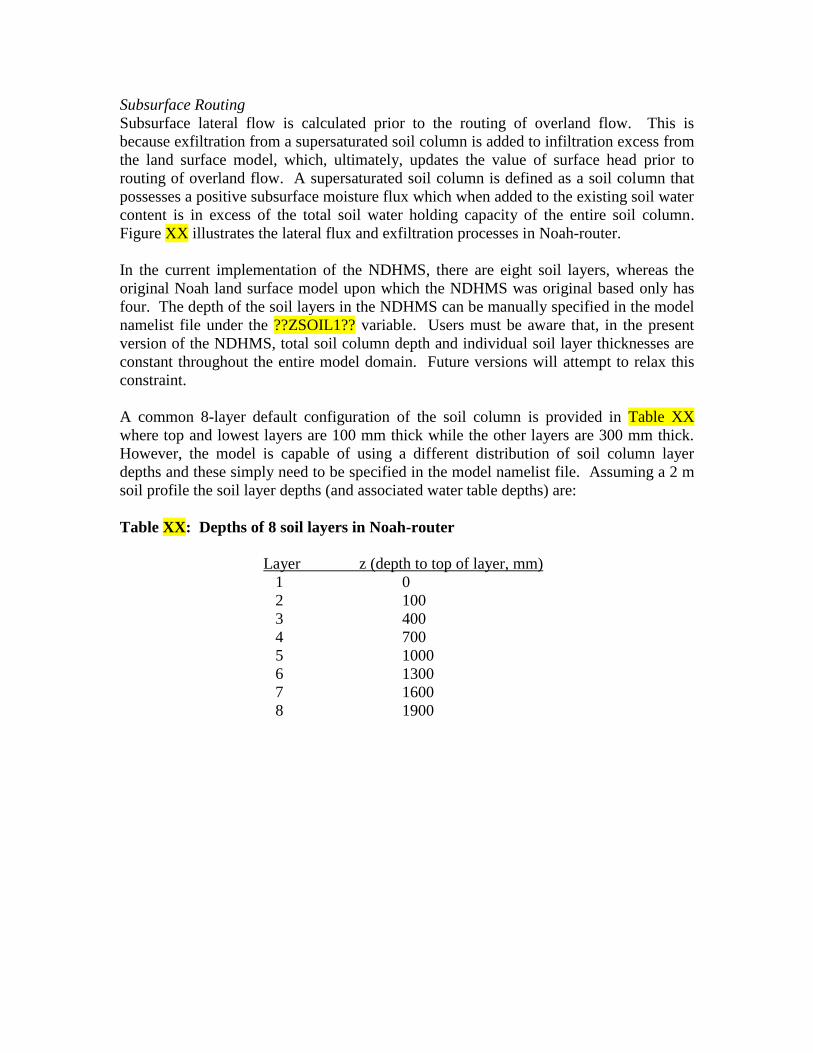
A common 8-layer default configuration of the soil column is provided in Table XX
where top and lowest layers are 100 mm thick while the other layers are 300 mm thick.
However, the model is capable of using a different distribution of soil column layer
depths and these simply need to be specified in the model namelist file. Assuming a 2 m
soil profile the soil layer depths (and associated water table depths) are:
Table XX: Depths of 8 soil layers in Noah-router
Layer z (depth to top of layer, mm)
1 0
2 100
3 400
4 700
5 1000
6 1300
7 1600
8 1900
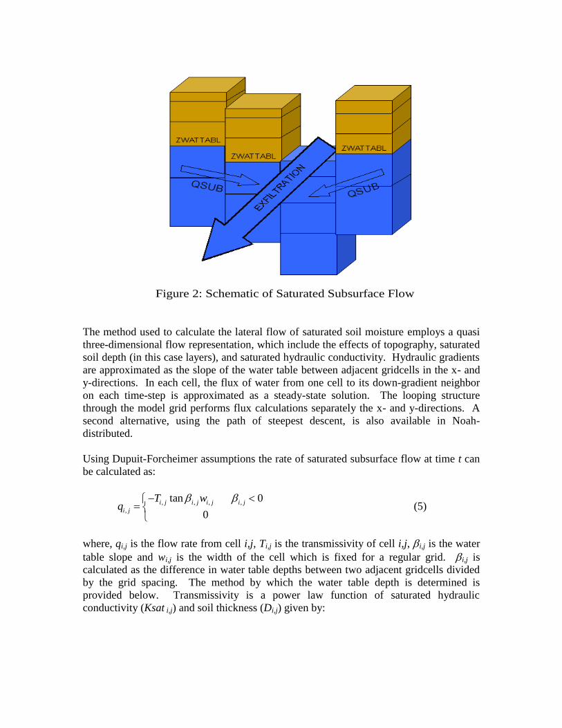
Figure 2: Schematic of Saturated Subsurface Flow Figure 2: Schematic of Saturated Subsurface Flow
The method used to calculate the lateral flow of saturated soil moisture employs a quasi
three-dimensional flow representation, which include the effects of topography, saturated
soil depth (in this case layers), and saturated hydraulic conductivity. Hydraulic gradients
are approximated as the slope of the water table between adjacent gridcells in the x- and
y-directions. In each cell, the flux of water from one cell to its down-gradient neighbor
on each time-step is approximated as a steady-state solution. The looping structure
through the model grid performs flux calculations separately the x- and y-directions. A
second alternative, using the path of steepest descent, is also available in Noah-
distributed.
Using Dupuit-Forcheimer assumptions the rate of saturated subsurface flow at time t can
be calculated as:
, , , ,
,
tan 0
0
i j i j i j i j
i j
T wq
(5)
where, qi,j is the flow rate from cell i,j, Ti,j is the transmissivity of cell i,j, i,j is the water
table slope and wi,j is the width of the cell which is fixed for a regular grid. i,j is
calculated as the difference in water table depths between two adjacent gridcells divided
by the grid spacing. The method by which the water table depth is determined is
provided below. Transmissivity is a power law function of saturated hydraulic
conductivity (Ksat i,j) and soil thickness (Di,j) given by:

, , ,
, ,, i,j ,
i,j i,j
1 z
0 z >D
i j i j i j
i j i ji j i j
Ksat D z
n DT D
(6)
where, zi,j is the depth to the water table. ni,j in Eq. (6) is defined as the local power law
exponent and is a tunable parameter that dictates the rate of decay of Ksati,j with depth.
When Eq. (6) is substituted into (5) the flow rate from cell i,j to its neighbor in the x-
direction can be expressed as
( , ) ( , ) , ( , ) 0x i j x i j i j when x i jq h (7)
where,
, , ,
( , ) ( , )
,
tani j i j i j
x i j x i j
i j
w Ksat D
n
(8)
,
,
,
,
1
i jn
i j
i j
i j
zh
D
(9)
This calculation is repeated for the y-direction when using the two-dimensional routing
method. The net lateral flow of saturated subsurface moisture (Qnet) for cell i,j then
becomes:
( , ) , ( , ) , ( , )net i j i j x i j i j y i j
x y
Q h h (10)
The mass balance for each cell on a model time step (t) can then be calculated in terms
of the change in depth to the water table (z):
( , )
( , )
( , )
1 net i j
i j
i j
Qz R t
A
(11)
where, is the soil porosity, R is the soil column recharge rate from infiltration or deep
subsurface injection and A is the grid cell area. In the NDHMS, R, is implicitly
accounted for during the land surface model integration as infiltration and subsequent soil
moisture increase. Assuming there is no deep soil injection of moisture (i.e. pressure
driven flow from below the lowest soil layer), R, in NDHMS is set equal to 0.
The methodology outlined in Equations 5-11 has no explicit information on soil layer
structure, as the method treats the soil as a single homogeneous column. Therefore,
changes in water table depth (z) can yield water table depths, which fall within a
particular soil layer. The NDHMS specifies the water table depth according the depth of
the top of the highest (i.e. nearest to the surface) saturated layer. The residual saturated
water above the uppermost, saturated soil layer is then added to the overall soil water
content of the overlying unsaturated layer. This computational structure requires
accounting steps to be performed prior to calculating Qnet.
Version 4.3 of the NDHMS introduces a model option to perform a fully-saturated
initialization and „drainage‟ simulation. This activity, activated through a switch () in the
model namelist file, conducts a long term-simulation where initial saturated soil
conditions are allowed to drain over time in response to gravitational flow. As such the
model is integrated forward in time and all land surface model and hydrological routing
physics are active. A drainage simulation capability is particularly useful for attempting
to develop subsequent initial conditions for unconfined aquifers within the model
domain. However, given the timescale for groundwater movement and limitations in the
model structure there is significant uncertainty in the „correctness‟ of such activities. The
main things to consider when conducting „drainage‟ simulation or „groundwater spinup‟
runs within the HDMS include 1) the specified depth of soil and number and thickness of
the soil vertical layers and 2) the prescription of the model bottom boundary condition.
Typically, for simulations with deep soil profiles (e.g. > 10m) the bottom boundary
condition is set to a „no-flow‟ boundary (SLOPETYP = 8) in the GENPARM.TBL
parameter file (see Appendix XX, for a description).

Terrain routing of overland flow
The terrain routing algorithms described below are found in
(module_Noah_distr_routing.F).
Overland flow in Noah-distributed is calculated using a fully-unsteady, explicit, finite-
difference, diffusive wave formulation (Figure 1) similar to that of Julien et al. (1995)
and Ogden et al. (1997). The diffusive wave equation, while slightly more complicated,
is, under some conditions, superior to the simpler and more traditionally used kinematic
wave equation, because it accounts for backwater effects and allows for flow on adverse
slopes. The overland flow routine described below can be implemented in either a 2-
dimensional (x and y direction) or 1-dimension (steepest descent or „D8‟) method. While
the 2-dimensional method may provide a more accurate depiction of water movement
across some complex surfaces it is more expensive in terms of computational time
compared with the 1-dimensional method. While the physics of both methods are
identical we have presented the formulation of the flow in equation form below using the
2-dimensional methodology.
Figure 1: Conceptual representation of terrain elements. Flow is routed across
terrain elements until it intersects a “channel” grid cell indicated by the blue line
where it becomes „in-flow‟ to the stream channel network.
The diffusive wave formulation is a simplification of the more general St. Venant
equations of continuity and momentum for a shallow water wave. The two-dimensional
continuity equation for a flood wave flowing over the land surface is
yx
e
qqhi
t x x
(1)
where, h is the surface flow depth; qx and qy are the unit discharges in the x- and y-
directions, respectively; and ie is the infiltration excess. The momentum equation used in
the diffusive wave formulation for the x-dimension is
fx ox
hS S
x
(2)
where, Sfx is the friction slope (or slope of the energy grade line) in the x-direction, Sox is
the terrain slope in the x-direction and h/x is the change in depth of the water surface
above the land surface in the x-direction.
In the 2-dimensional option, flow across the terrain grid is calculated first in the x- then
in the y-direction. In order to solve Eq. 1 values for qx and qy are required. In most
hydrological models they are typically calculated by use of a resistance equation such as
Manning‟s equation or the Chezy equation, which incorporates the expression for
momentum losses given in Eq. 2. In the NDHMS, a form of Manning‟s equation is
implemented:
x xq h (3)
where,
1 25
;3
fx
x
OV
S
n (4)
where, nOV is the roughness coefficient of the land surface and is a tunable parameter and
is a unit dependent coefficient expressed here for SI units.
The overland flow formulation has been used effectively at fine terrain scales ranging
from 30-1000 m. There has not been rigorous testing to date, in the NDHMS, at larger
length-scales (> 1 km). This is due to the fact that typical overland flood waves possess
length scales much smaller than 1 km. Micro-topography can also influence the behavior
of a flood wave. Correspondingly, at larger grid sizes (e.g. > 500 m) there will be poor
resolution of the flood wave and the small-scale features that affect it. Also, at coarser
resolutions, terrain slopes between gridcells are lower due to an effective smoothing of
topography as grid size resolution is decreased. Each of these features will degrade the
performance of dynamic flood wave models to accurately simulate overland flow
processes. Hence, it is generally considered that finer resolutions yield superior results.
The selected model time step is directly tied to the grid resolution. In order to prevent
numerical diffusion of a simulated flood wave (where numerical diffusion is the artificial
dissipation and dispersion of a flood wave) a proper time step must be selected to match
the selected grid size. This match is dependent upon the assumed wave speed or celerity
(c). The Courant Number, Cn= c(t/x), should be close to 1.0 in order to prevent
numerical diffusion. The value of the Cn also affects the stability of the routing routine
such that values of Cn should always be less than 1.0. Therefore the following model
time steps are suggested as a function of model grid size:

Table 1: Suggested routing time steps for various grid spacings
x (m) t (s)
30 2
100 6
250 15
500 30
1000 60
The overland flow routing option is activated using a switch parameter (OVRTSWTCH)
in the NDHMS model namelist. If activated the following terrain fields and model
namelist parameters must be provided:
Terrain grid or Digital Elevation Model (DEM) Note: this grid may provided
at resolutions equal to or finer than the native land model resolution
Channel network grid identifying the location of stream channel grid cells
Specification of the routing grid cell spacing (DXRT), routing grid time step
(DTRT) and subgrid aggregation factor (AGGFACTR-defined as the ratio of
the subgrid resolution to the native land model resolution, see Section XXXX
above.)
Channel Inflow
Currently there is no explicit sub-grid representation of overland flow discharging into a
stream channel. Instead, a simple mass balance calculation is performed. Inflow to
stream channels occurs when the ponded water depth (or surface head, „SFHEADRT‟) of
stream channel grid cells exceeds a pre-defined retention depth („RETDEPRT‟). As
indicated above, the depth of surface head on any grid cell is a combination of the local
infiltration excess, the amount of water flowing onto the grid cell from over land flow,
and exfiltration from groundwater flow (described below). The quantity of surface head
in excess of the retention depth is accumulated as stream channel inflow and is added to
the channel routing routine (described below).
When routing is activated any overland flow in excess of the local retention depth,
reaching a stream channel grid cell will be effectively „discharged‟ into the stream
channel network. In the NDHMS, values of „channel inflow‟ are accumulated on the
channel grid. Users can keep track of the total channel network channel inflow volume
by setting the namelist file option „HIRES_OUT‟ = 1, which produces an ASCII-
formatted timeseries file of channel inflow volume in units of millions of cubic meters
(Mm3). The name of the file produced will be „chan_inflow.txt‟ and it will be written to
the local run directory. Users can also output the spatial distribution of channel inflow on
a high-resolution, netcdf-formatted terrain grid along with the „chan_inflow.txt‟ file by
setting the HIRES_OUT = 2 in the model namelist file.

Stream and River Channel routing
The channel routing module (module_Noah_channel_routing.F) allows for the one-
dimensional, distributed routing of streamflow across the domain. An optional, switch-
activated, level-pool lake/reservoir algorithm is also available and is described below.
Channel routing is performed on a pixel-by-pixel basis along a predefined channel
network grid that is input to the model within the high-resolution terrain routing grid file
(see Section XXX for details). Within each channel grid cell there is an assumed channel
reach of trapezoidal geometry as depicted in Figure XX. Channel parameters side slope,
bottom width and roughness are currently prescribed as functions of Strahler stream order
which is also input within the high-resolution terrain routing grid file. As discussed
above in Section XX, channel elements receive lateral inflow from overland flow. There
is currently no overbank flow so flow into the channel model is effectively one-way and
the vertical dimension of the channel is effectively infinite. Future enhancements will
attempt to relax these assumptions. Therefore, the NDHMS does not presently explicit
represent inundation areas. Uncertainties in channel geometry parameters and the lack of
an overbank flow representation result in significant uncertainty for users wishing to
compare model flood stages versus those from observations. It is strongly recommended
that users compare model versus observed streamflow discharge values and use observed
stage-discharge relationships or „rating curves‟ when wishing to relate modeled/predicted
streamflow values to actual river levels and potential inundation areas.
Channel Slope, So
Channel Length, x (m)
Channel side slope, z (m)
Constant bottom width, Tb (m)
Manning‟s roughness coefficient, n
Figure XX: Schematic of Channel Routing Terms
Channel flow down through the gridded channel network is performed using an implicit,
one-diemnsional, variable time-stepping diffusive wave formulation. As mentioned
above in Section XX, the diffusive wave formulation is a simplification of the more
1
z
Tb
So n
x
Q
h
Q‟
h‟
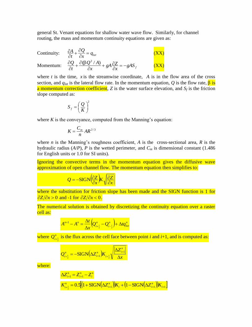
general St. Venant equations for shallow water wave flow. Similarly, for channel
routing, the mass and momentum continuity equations are given as:
Continuity: latqx
Q
tA
(XX)
Momentum: fgASxZgA
x
AQ
t
Q
)/( 2
(XX)
where t is the time, x is the streamwise coordinate, A is in the flow area of the cross
section, and qlat is the lateral flow rate. In the momentum equation, Q is the flow rate, is
a momentum correction coefficient, Z is the water surface elevation, and Sf is the friction
slope computed as:
2
K
QS f
where K is the conveyance, computed from the Manning‟s equation:
3/2ARn
CK m
where n is the Manning‟s roughness coefficient, A is the cross-sectional area, R is the
hydraulic radius (A/P), P is the wetted perimeter, and Cm is dimensional constant (1.486
for English units or 1.0 for SI units).
Ignoring the convective terms in the momentum equation gives the diffusive wave
approximation of open channel flow. The momentum equation then simplifies to:
xZK
xZQ
SIGN
where the substitution for friction slope has been made and the SIGN function is 1 for
0 xZ and -1 for 0 xZ .
The numerical solution is obtained by discretizing the continuity equation over a raster
cell as:
n
lat
n
i
n
i
nn tqQQx
tAA
21
21
1
where n
iQ
21 is the flux across the cell face between point i and i+1, and is computed as:
x
ZKZQ
n
i
i
n
i
n
i
1
121
21 SIGN
where:
n
i
n
i
n
i ZZZ 11
111 SIGN1SIGN15.021
i
n
ii
n
i
n
iKZKZK

Presently a first-order, Newton-Raphson (N-R) solver is used to integrate the diffusive
wave flow equations. Under certain streamflow conditions (e.g. typically low gradient
channel reaches) the first-order solver method can produce some instabilities resulting in
numerical oscillations in calculated streamflow values. To address this issue, higher
order solver methods will be implemented in future versions of the NDHMS.
Variable time-stepping in the diffusive wave channel routing module in order to satisfy
Courant constraints and avoid numerical dispersion and instabilities in the solutions.
Unlike typical overland flow flood waves which have very shallow flow depths, on the
order of millimeters or less, channel flood waves have appreciably greater flow depths
and wave amplitudes, which can potentially result in strong momentum gradients and
strong accelerations in a propagating wave. To properly characterize the dynamic
propagation of such highly variable flood waves it is often necessary to decrease model
time-steps in order to satisfy Courant conditions. Therefore the NDHMS utilizes a
variable time-step methodology. The initial value of the channel routing time-step is set
equal to that of the overland flow routing timestep which is a function of grid spacing. If,
during model integration the N-R convergence criteria for upstream-dowsntream
streamflow discharge values is not met, the channel routing time-step is decreased by a
factor of one-half and the N-R solver is called again.
It is important to note that use of variable time-stepping can significantly affect model
computational performance resulting in much slower solution times for rapidly evolving
streamflow conditions such as those occurring during significant flood events. Therefore,
selection of the time-step decrease factor (default value set to 0.5) and the N-R
convergence criteria can each affect model computational performance.
Uncertainty in channel routing parameters also can have a significant impact on the
accuracy of the model solution which implies that model calibration is often required
upon implementation in a new domain. Presently, all of the channel routing parameters
are prescribed as functions of stream order in a channel routing parameter table
„CHANPARM.TBL‟. The structure of this file is described in detail in Section XX. It
should be noted that prescription of channel flow parameters as functions of stream order
is likely to be a valid assumption over relatively small catchments and not over large
regions. Future versions of the NDHMS will incorporate options to prescribe spatially
distributed channel routing parameters (side slope, bottom width and roughness) within
the high-resolution terrain routing grid file.
The channel flow routing option is activated using a switch parameter (CHRTSWTCH)
in the NDHMS model namelist. If activated the following terrain fields and model
namelist parameters must be provided:
Terrain grid or Digital Elevation Model (DEM) Note: this grid may provided
at resolutions equal to or finer than the native land model resolution
Channel network grid identifying the location of stream channel grid cells
Strahler stream order grid identifying the stream order for all channel pixels
within the channel network

Channel flowdirection grid. This grid explicitly defines flow directions along
the channel network.
Optional: Forecast point grid. This grid is a grid of selected channel pixels for
which channel discharge and flow depth are to be output within a netcdf point
file and an ASCII timeseries file.
Lake/Reservoir Routing Module:
A simple mass balance, level-pool lake/reservoir routing module allows for an estimate
of the inline impact of small and large reservoirs on hydrologic response. A
lake/reservoir or series of lakes/reservoirs are identified in the channel routing network,
and lake/reservoir storage and outflow are estimated using a level-pool routing scheme.
The only conceptual difference between lakes and reservoirs as represented in the
NDHMS is that reservoirs contain both orifice and weir outlets for reservoir discharge
while lakes only contain weirs.
Fluxes into a lake/reservoir object occur through the channel network and when surface
overland flow intersects a lake object. Fluxes from lake/reservoir objects are made only
through the channel network and no fluxes from lake/reservoir objects to the atmosphere
or the land surface are currently represented (i.e. there is currently no lake evaporation or
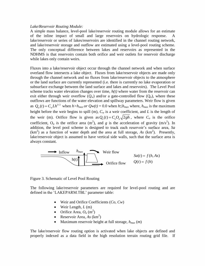
subsurface exchange between the land surface and lakes and reservoirs). The Level Pool
scheme tracks water elevation changes over time, h(t) where water from the reservoir can
exit either through weir overflow (Qw) and/or a gate-controlled flow (Qo), where these
outflows are functions of the water elevation and spillway parameters. Weir flow is given
as 3/ 2( )w wQ t C Lh when h>hmax or Qw(t) = 0.0 when h≤hmax where, hmax is the maximum
height before the weir begins to spill (m), Cw is a weir coefficient, and L is the length of
the weir (m). Orifice flow is given as ( ) 2o o aQ t C O gh , where Co is the orifice
coefficient, Oa is the orifice area (m2), and g is the acceleration of gravity (m/s
2). In
addition, the level pool scheme is designed to track each reservoir‟s surface area, Sa
(km2) as a function of water depth and the area at full storage, As (km
2). Presently,
lake/reservoir object is assumed to have vertical side walls, such that the surface area is
always constant.
Figure 3. Schematic of Level Pool Routing
The following lake/reservoir parameters are required for level-pool routing and are
defined in the „LAKEPARM.TBL‟ parameter table:
Weir and Orifice Coefficients (Co, Cw)
Weir Length, L (m)
Orifice Area, Oa (m2)
Reservoir Area, As (km2)
Maximum reservoir height at full storage, hmax (m)
The lake/reservoir flow routing option is activated when lake objects are defined and
properly indexed as a data field in the high resolution terrain routing grid file. If
Weir flow
Orifice flow h(t)
Inflow ( ) ( , )
( ) ( )
Sa t f h As
Q t f h
hmax

lake/reservoir objects are present in the lake grid (and also within the channel network)
then routing through those objects will occur. There are several special requirements for
the lake grid and channel routing grids when lakes/reservoirs are to be represented and
these are discussed in detail in Section XXX. The following input data variables and
parameter files are required for level-pool routing:
LAKEPARM.TBL parameter file (described in the Appendix)
LAKEGRID
CHANNELGRID
Conceptual Baseflow Model Description
Aquifer processes contributing baseflow often operate at depths greater than well below
ground surface. As such, there are often conceptual shortcomings in current land surface
models in their representation of groundwater processes. Because these processes
contribute to streamflow (typically as „baseflow‟) a parameterization is often used in
order to simulate total streamflow values that are comparable with observed streamflow
from gauging stations. Therefore, a switch-activated baseflow module
„module_Noah_gw_baseflow.F‟ has been created which conceptually (i.e. not physically-
explicit) represents baseflow contributions to streamflow. This model option is
particularly useful when the NDHMS is used for long-term streamflow
simulation/prediction and baseflow or „low flow‟ processes must be properly accounted
for. Besides potential calibration of the Noah land surface model parameters the
conceptual baseflow model does not directly impact the performance of the land surface
model scheme. The new baseflow module is linked to the NDHMS through the discharge
of „deep drainage‟ from the land surface soil column (sometimes referred to as
„underground runoff‟). The basic methodology employed into NDHMS is described
below along with results from some preliminary sensitivity tests for the Santee River
basin.
The baseflow parameterization in the NDHMS uses spatially-aggregated drainage from
the soil profile as recharge to a conceptual groundwater reservoir (Fig. XX). The unit of
spatial aggregation is often taken to be that of a sub-basin within a watershed where
streamflow data is available for the sub-basin. Each sub-basin has a groundwater
reservoir („bucket‟) with a conceptual depth and associated conceptual volumetric
capacity. The reservoir operates as a simple bucket where outflow (= „baseflow‟ or
„stream inflow‟) is estimated using an empirically-derived function of recharge. The
functional type and parameters are determined empirically from offline tests using the
estimated of baseflow from stream gauge observations and model-derived estimates of
bucket recharge provided by the NDHMS. Presently, the NDHMS uses an exponential
function (See Fig. XX) for estimating the bucket discharge as a function of a conceptual
depth of water in the bucket. Note that because this is a highly conceptualized
formulation that the depth of water in the bucket in no way infers the actual depth of
water in a real aquifer system. Estimated baseflow discharged from the bucket model is
then combined with lateral inflow from overland flow from Noah-distributed and is input
directly into the stream network as „stream inflow‟. Presently, the total basin baseflow
flux to the stream network is equally distributed among all channel pixels within a basin.
Lacking more specific information on regional groundwater basins, the
groundwater/baseflow basins in the NDHMS are assumed to match those of the surface
topography.
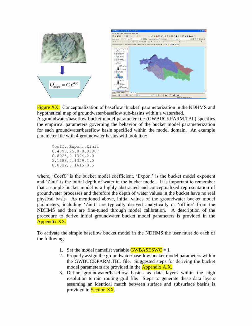
Figure XX: Conceptualization of baseflow „bucket‟ parameterization in the NDHMS and
hypothetical map of groundwater/baseflow sub-basins within a watershed.
A groundwater/baseflow bucket model parameter file (GWBUCKPARM.TBL) specifies
the empirical parameters governing the behavior of the bucket model parameterization
for each groundwater/baseflow basin specified within the model domain. An example
parameter file with 4 groundwater basins will look like:
Coeff.,Expon.,Zinit
0.4898,25.0,0.03867
0.8925,0.1394,2.0
2.1388,0.1359,1.0
0.0332,0.1615,0.5
where, „Coeff.‟ is the bucket model coefficient, „Expon.‟ is the bucket model exponent
and „Zinit‟ is the initial depth of water in the bucket model. It is important to remember
that a simple bucket model is a highly abstracted and conceptualized representation of
groundwater processes and therefore the depth of water values in the bucket have no real
physical basis. As mentioned above, initial values of the groundwater bucket model
parameters, including „Zinit‟ are typically derived analytically or „offline‟ from the
NDHMS and then are fine-tuned through model calibration. A description of the
procedure to derive initial groundwater bucket model parameters is provided in the
Appendix XX.
To activate the simple baseflow bucket model in the NDHMS the user must do each of
the following:
1. Set the model namelist variable GWBASESWC = 1
2. Properly assign the groundwater/baseflow bucket model parameters within
the GWBUCKPARM.TBL file. Suggested steps for deriving the bucket
model parameters are provided in the Appendix A.X.
3. Define groundwater/baseflow basins as data layers within the high
resolution terrain routing grid file. Steps to generate these data layers
assuming an identical match between surface and subsurface basins is
provided in Section XX.
i iz
basei iQ C e
i iz
basei iQ C e

If activated, three ASCII-formatted, time-series, output files are generated by the bucket
model parameterization that contain timeseries values of the flow into the bucket
(„gw_inflow.txt‟), flow out of the bucket („gw_outflow.txt‟) and the conceptual depth of
water in the groundwater/baseflow bucket („gw_zlev.txt‟).

Model Technical Description and User Guide
This portion of the document presents the technical description of the NDHMS model
code including:
1. Coding structure and programming conventions
2. Directory structures
3. Description of modules
4. Setup and execution of uncoupled NDHMS code
5. Setup and execution of coupled WRF-NDHMS code
6. Setup of model domain grids
The following, final section of the document presents the NDHMS input and output data
structures and descriptions of the various model namelists and parameter tables.

1. Coding Structure and Programming Conventions
The NDHMS is written in a modularized, Fortran90 coding structure whose routing
physics modules are switch activated through a single model namelist file. The code has
been parallelized for execution on high-performance, parallel computing architectures
including LINUX commodity clusters and multi-processor desktops as well as the IBM
blue gene supercomputers.
The code has been compiled using the Portland Group FORTRAN (for use with Linux-
based operating systems on desktops and clusters) and the IBM IFORT FORTRAN
compilers (for supercomputers).
Because the NDHMS relies on NETCDF input and output file conventions, NETCDF
FORTRAN libraries must be installed and properly compiled on the system upon which
the NDHMS is to be executed. Not doing so will result in error numerous „…undefined
reference to netcdf library …‟ messages upon compilation.
Parallelization of the NDHMS code utilizes domain decomposition and „halo‟ array
passing structures similar to those used in the WRF atmospheric model. Message passing
between processors is accomplished using „MPICH‟ protocols. Therefore the relevant
„mpich‟ libraries must be installed and properly compiled on the system upon which the
NDHMS is to be executed in parallel mode. Separate compilations, and therefore
executables, of the NDHMS code are required
(See Section XXX for a „Steps to Install‟ and „Quick Start‟ guide of procedures required
to install and run the NDHMS in each sequential, parallel and WRF-coupled modes).

2. Directory Structures
The top level directory structure of the code is provided below and Subdirectory
structures are described thereafter. Code descriptions in bold italics indicate code that is
relevant to routing modeling and/or more frequently modified routines.
„v4.3/‟ directory:
This is the top level directory present immediately following untarring of the NDHMS
file tar package.
arc/ ???
batch.csh - c-shell script to compile code
Makefile - top-level makefile
IO_code/ - directory containing most of model code
macros/ - directory containing selected compile options
MPP/ - directory containing parallel model code
Noah_code/ - model code (utilities and global parameter settings)
Run/ - directory containing model executable once
compiled wrf/ ???
WRF_code/ - directory containing Noah LSM code and other modules
„IO_code/‟ directory:
This directory contains the model drivers, the model input/output modules and most of
the model physics modules related to routing.
drive_rtland.F - surrogate land model driver used when coupled
to WRF
DRIVE_RTLAND.F - surrogate land model driver used when coupled to
WRF
Makefile - IO_code directory makefile
module_Noah_channel_routing.F - model physics module for channel routing
module_Noah_chan_param_init_rt.F - module for initializing channel parameters
module_Noah_distr_routing.F - model physics module for terrain routing
module_Noah_grads_output.F - OBSOLETE
module_Noah_gw_baseflow.F - model physics module for gw/baseflow
module_Noahlsm_hrldas_input.F - OBSOLETE
module_Noahlsm_wrf_input_rt.F - module for most input/output
module_RTLAND.F - main model driver
Noah_driver.F - OBSOLETE
Noah_driver_hrldas.F - OBSOLETE
Noah_driver_rtfdda.F - OBSOLETE
Noah_driver_wrfcode.F - high level driver
„WRF_code/‟ directory:
This directory contains the Noah LSM.
Makefile - Noah LSM makefile
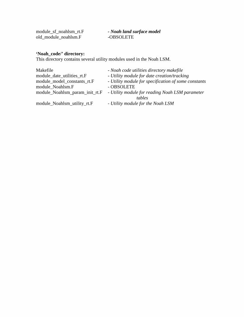
module_sf_noahlsm_rt.F - Noah land surface model
old_module_noahlsm.F -OBSOLETE
„Noah_code/‟ directory:
This directory contains several utility modules used in the Noah LSM.
Makefile - Noah code utilities directory makefile
module_date_utilities_rt.F - Utility module for date creation/tracking
module_model_constants_rt.F - Utility module for specification of some constants
module_Noahlsm.F - OBSOLETE
module_Noahlsm_param_init_rt.F - Utility module for reading Noah LSM parameter
tables
module_Noahlsm_utility_rt.F - Utility module for the Noah LSM

3. Description of Physics Modules
The basic structure of the NDHMS is diagrammatically illustrated in Figure XX. High
level job management is handled by the land model driver, which has previously been
referred to as the NCAR High Resolution Land Data Assimilation System (HRLDAS).
Upon initialization static land surface and terrain data are read into the land model driver
and the model domain and computational arrays are established. Next forcing data is
read in. As the model integrates in time the calling structure of the physics modules
proceeds as 1) the 1-D, gridded land surface model, 2) disaggregation to the high
resolution terrain routing grids (if routing is activated), 3) sub-surface and surface routing
(if active), 4) the conceptual baseflow model (if active), 5) channel and reservoir routing
(if active), 6) aggregation from the high resolution terrain routing grid to the land surface
model grid (if routing is active). Results from these integrations are then written to the
model output files or, in the case of a coupled WRF-NDHMS simulation, passed back to
the WRF model.
HRLDAS
Land
Model
Driver/
Coupler
Geographic/hydrographic
data layers
Noah/CLM land surface models
(LSMs)
Spatial disaggregation to
routing grid
Terrain routing: surface
and subsurface
Channel and reservoir routing
Baseflow module
Spatial aggregation to
LSM grid
HRLDAS
Land
Model
Driver/
Coupler
Geographic/hydrographic
data layers
Noah/CLM land surface models
(LSMs)
Spatial disaggregation to
routing grid
Terrain routing: surface
and subsurface
Channel and reservoir routing
Baseflow module
Spatial aggregation to
LSM grid

4. Setup and execution of uncoupled NDHMS
This section provides a highly abridged presentation of the most essential steps for setting
up and running the model leaving the details of each step to the relevant chapters. As
such this short „Quick Start‟ should only be used as a reference or for those desiring to
perform the simplest of simulations. The steps below assume that the appropriate netcdf
libraries and, if parallel-processing is desired, multi-processing software have been
installed. Model runs that do not involve changes to the model code can be set up almost
entirely from the v4.3/ and Run/ directories.
There are 5 main steps to installing and executing Noah-distributed: (Additional
installation information is provided in Chapter XXXX.)
i) Assign proper NETCDF and Makefile settings The first step to installing the
NDHMS is to set up appropriate links to netdf INCLUDE and LIB directories. While
different methods and options exist on different systems and example of how this can
easily be done is as follows:
a. Create a netcdf/ directory in the home directory
b. Cd to ~/netcdf/
c. Create a symbolic link to the netcdf INCLUDE and LIB directories that
should be present (already installed) on the system/network:
For example: % ln –sf /opt/netcdf/* .
This should create the following symbolic links in the ~/netcdf/ directory:
bin -> /opt/netcdf/bin
include -> /opt/netcdf/include
lib -> /opt/netcdf/lib
share -> /opt/netcdf/share
It is also essential to verify that all additional compiler, netcdf and makefile environment
variables required to compile the model are properly specified. These environment
variables are specified in the v4.3/macros file are properly linked (e.g. COMPILER90,
CPP, NETCDFINC, NETCDFLIB)
ii) Compiling the model. This is done by running the „batch.csh‟ c-shell script in the
v4.3/ directory. The user will be prompted for which type of model run is to be
performed and, therefore, which type of executable will be created.
%csh batch.csh
Please select from following supported options.
1. Linux PGI compiler sequential
2. Linux PGI compiler mpp
3. Linux PGI compiler sequential, with boundary check
4. IBM AIX compiler sequential, xlf90_r

5. IBM AIX compiler mpp
6. Linux PGI compiler mpp, lib only (to be coupled with WRF)
0. exit only
Enter selection [1-5] :
Most users will be using options 1 (for single processor, sequential runs) or 2 (parallel
processor runs) on typical LINUX machines. Option 3 simply contains additional
runtime boundary checks which is useful for debugging. Options 4 and 5 are available if
the IBM AIX compiler is used (Use this for NCAR IBM supercomputers such as
„bluefire‟). Option 6 will be used when the Noah-distributed hydrological model will be
coupled to WRF and run on a LINUX platform.
Successful compilation of options 1-5 will result in the creation of a new model
executable which resides within the v4.3/Run directory. For sequential and parallel runs
the executables will be, respectively:
Noah_wrfdriver_beta (sequential)
Noah_wrfdriver_beta_mpp (parallel)
NOTE: If there are compilation errors, oftentimes error messages will be provided with
module names and line numbers. These module line numbers are ONLY relevant to
lowercase (*.f) files and NOT uppercase (*.F) files. Since the *.f files are scrubbed
within the Makefile upon compilation they are not available to view. To not scrub the .f
files one needs to make the appropriate edit to the appropriate Makefile. This means
determining which make file needs to be edited and commenting out the „rm *.f‟ line
under the appropriate module.
Be sure to check the date on this executable to make sure that you have compiled
successfully. If you experience problems compiling or if it is your first time compiling
you might try typing 'make clean' to remove old object files. So far the Noah-distributed
has been successfully compiled only on LINUX platforms.
Once the proper model executable file has been created users will need to create and
populate a run directory from which the model will be executed. All of the appropriate
parameter tables, model namelist file and model executable need to be placed in this
directory. An example of listing of these files is provided in the „example_FRNG/‟
directory contained within the Run/ directory.
ii) Create/place routing files in a /terrain/ directory. Place the LSM terrain grid file
(a.k.a. „geogrid_d0X.nc‟) and, if routing is to be performed, the high-resolution netcdf
terrain grid into this terrain/ directory. Construction of these netcdf files is described in
Chapter XXXX.
iii) Create/place forcing data files in /forcing/ directory. These are the data that “drive”
the hydrologic simulation. Noah-d uses a netcdf I/O convention similar to the Weather
Research and Forecasting model and, therefore, it is fairly easy to adapt WRF output to
drive Noah-d. There are seven meteorological variable that are required: 2 m air
temperature, 2 m specific humidity, 10 wind speed (u and v components), surface
pressure, precipitation rate, incoming short and longwave radiation. These variables are
stored within a single netcdf file where one file is specified for each model time-step.
Specific details on the untis and formate of these data at given in Chapter XXXX. These
data need to be placed in the forcing/ directory.
iv) Edit the namelist. Open and edit 'noah_wrfcode.namelist' to set up a simulation to
your specifications. The namelist is fairly well commented. The directory for input
forcing data must be specified (INDIR), as must the pathway and filename to the
WRFSTATIC file (WRFSI_STATIC_FLNM) and type of forcing data (FORC_TYP). Be
sure to activate only those routing switches for which you have the required data. Routing
timestep 'DTRT' must be set in accordance with the routing grid spacing in order to
satisfy Courant constraints (see Chapter XXXX for a discussion on Courant constraints).
Be sure to include the full path and directory when specifying Routing Input Files.
Description of the terms in the namelist are given in Chapter XXXX.
v) Execute the model. Type './Noah_wrfdriver_beta' at the command line to execute the
sequential version the model. For parallel runs the command may differ according the
specifications of the parallel-processing software on individual machines but a common
execution command may look like „mpirun –np # Noah_wrfdriver_beta_mpp‟, where # is
the number of processors to be used. If run successfully, output will be generated as a
series of netcdf files with associated time and date information in the filenames. Users
seeking to perform simulations where the Noah-distributed model is coupled to WRF
should refer to Chapter XXXX.

5. Setup and execution of the coupled WRF-NDHMS
(see/update document and get material from ppt slides)
Before beginning, make sure that both uncoupled WRF model and the uncoupled version
of the Noah-distributed/NDHMS have been properly installed, configured, compiled and
executed on the desired system. It will be much easier to debug problems with the
coupled model once each component of the uncoupled models have been properly
installed compiled and executed. Also, if any changes or model developments are made
to the Noah-distributed model (such as routing functions or I/O modules) it is strongly
suggested that you recompile and perform test executions of the uncoupled Noah-
distributed run in offline mode before attempting to directly perform a coupled model
simulation. These steps will help ensure that the coupled version will compile and
execute successfully and will help with troubleshooting any problems that may arise.
To install, compile and execute the coupled WRF/NDHMS do the following:
1) Obtain, unzip and unpack the coupled model tarfile
2) Upon first installation or if you change something in the Noah-distributed
portion of the coupled model, recompile and test the uncoupled model:
a) Under WRF_COUPLE/phys/RTLAND, run "csh batch.csh", and choose option 2
(Linux mpp option). Successful completion of this step will create an
„uncoupled‟ Noah-distributed/NDHMS model executable set up to run in parallel
mode.
b) Copy or link the WRF_COUPLE/phys/RTLAND/Run/Noah_wrfdriver_beta_mpp
to WRF_COUPLE/run/RT (This RT directory is where the Noah-distributed
model is executed from in both uncoupled and coupled modes.) Make sure that
all the necessary Noah-d/NDHMS files (e.g. .TBL and namelist files) are there.
c) Test the stand alone there as if it were a normal simulation. You can test using
previous WRF output (FORC_TYP=2 in the namelist) or with constant/idealized
forcing (FORC_TYP=4). Execute the model using a typical NDHMS execution:
command for parallel systems. (e.g. „mpirun –np 8 Noah_wrfdriver_beta_mpp >
log.txt &)
d) Once the model successfully runs in uncoupled mode proceed to Step #3.
3) If above passed, you want to run couple. Do following: a) Clean out all old compiles from both WRF and the uncoupled model. Goto the
„WRF_COUPLE/‟ directory and type „clean –a‟ (this should clear all old
executables, libraries, object files, etc.)
b) Under „WRF_COUPLE/phys/RTLAND‟:
i) Perform a „make clean‟ and remove all old exectuables in
„WRF_COUPLE/phys/RTLAND/Run/‟
ii) As in step 2a above, run "csh batch.csh", and choose 6. (This setting will
compile the Noah-distributed model for coupling to WRF. This compile
WILL NOT generate an executable but will instead generate a new library file
called „librtland.a‟ so that "compile em_real" can compile the file as part of its
full WRF compile.
c) cd to „WRF_COUPLE/main/‟ and double check to remove any
„WRF_COUPLE/main/*.exe‟ files
d) Under „WRF_COUPLE/‟, execute „./compile em_real‟ to make a complete new
wrf.exe which will have the Noah-distributed library compiled within. You will
need to select the proper compile option based on your individual system.
Usually this will be a distributed memory, parallel compile („dmpar‟). As with a
typical WRF compile this will take several minutes to complete.
e) If successful a new „wrf.exe‟ executable file will be created in
„WRF_COUPLE/main/‟. Copy or link this executable to the directory where you
will run the coupled WRF/Noah-d model such as the „WRF_COUPLE/run/
„directory. It is also a good idea to give a new name for the coupled model
executable to distinguish it from regular „uncoupled‟ wrf.exe executable files (e.g.
„wrf_couple.exe‟).
f) If not already present, create a „RT/‟ directory in the „WRF_COUPLE/run/‟
directory. Make sure that all of the usual Noah-d files (.TBLs and Noah-d
namelist files) are there. Edit the namelist such that FORC_TYP=2 so that the
NDHMS will assume WRF-formatted forcing data. However, the „INDIR‟
variable in the namelist becomes irrelevant for coupled WRF/NDHMS runs.
g) Link the „noah_wrfcode_namelist‟ from „RT/‟ into the „WRF_COUPLE /run/‟
directory so that WRF will find these upon execution.
h) Execute the model using a typical wrf execution command for parallel systems.
e.g. mpirun –np 16 wrf_couple.exe > log.txt &

6. Domain Processing
a. General Overview
Utilizing the netcdf data convention, there are two files that need to be created in
order to run the NCAR distributed hydrological modeling system (NDHMS). The
two files specify the data layers that are used for modeling on the land surface model
grid (or coarse grid) and the terrain routing grid (or high-resolution grid). Data
contained in the land surface model grid is highly dependent upon the specific land
surface model (LSM) used in the NDHMS. As of the preparation of this document
only the Noah LSM (Ek et al., 2003, Mitchell et al. 200X) has been coupled into the
NDHMS though future versions may incorporate additional LSMs such as the
Community Land Model (CLM, Oleson et al., 200X). Conversely, because of the
modular structure of the NDHMS, data for the terrain routing grid should remain
fairly consistent even when different LSMs are coupled into the system. Lastly,
preparation of the LSM grid and the terrain grid are required and these grids are the
same, whether or not the NDHMS is executed in a coupled mode with the Weather
Research and Forecasting (WRF) model. In the sections below, the data requirements
for model execution are provided as are an example set of processing steps that would
create the required LSM and terrain routing grids. The last two sections describe the
required attributes that must be specified, via parameter tables, to enable channel
routing, reservoir routing and a simple baseflow parameterization.
One key requirement in setting up the LSM and terrain grids is that the spatial extent
of the two grids must be identical and that the spatial resolution of the terrain grid
must be an integer multiple of the LSM grid. This is because the terrain grid operates
on a fine mesh overlain onto the LSM and that in the NDHMS selected model state
and flux variables are disaggregated/aggregated between the LSM and terrain grids.
This internal nesting in Gochis and Chen (2003) allows the LSM to run at one spatial
resolution while the terrain and stream channel routing routines are executed on a
much more finely resolved grid. While the model can operate when both grids have
equal spatial resolution (e.g. 100m or finer) this sub-grid nesting capability is
particularly useful in minimizing computational demands when the NDHMS is
coupled to WRF.
b. Land Surface Model Grid Setup
The data required to execute a spatially-distributed, or gridded, 1-dimensional
(vertical) LSM is specified on the Land Surface Model grid (hereafter referred to as
the „LSM grid‟ data file). The data contained within LSM grid data file are
dependent on the specific choice of LSM used in the NDHMS. In this section, we
will use the example of the Noah LSM as this model has already been coupled to the
NHDMS and because this model is already coupled into the WRF model. First, use
of the WRF pre-processor „geogrid‟ to build the LSM grid data file will be discussed.
The „geogrid‟ tool is extremely useful since it automates the entire procedure of
defining in space, geo-referencing and attributing most of the land surface parameter
data required to execute the Noah LSM. Users familiar with the WRF model or
desiring to run the NHDMS coupled to the WRF model will most likely use this
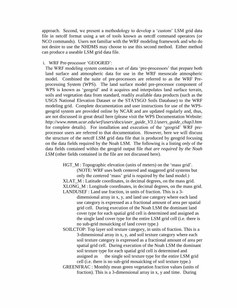
approach. Second, we present a methodology to develop a „custom‟ LSM grid data
file in netcdf format using a set of tools known as netcdf command operators (or
NCO commands). Users not familiar with the WRF modeling framework and who do
not desire to use the NHDMS may choose to use this second method. Either method
can produce a useable LSM grid data file.
i. WRF Pre-processor „GEOGRID‟:
The WRF modeling system contains a set of data „pre-processors‟ that prepare both
land surface and atmospheric data for use in the WRF mesoscale atmospheric
model. Combined the suite of pre-processors are referred to as the WRF Pre-
processing System (WPS). The land surface model pre-processor component of
WPS is known as „geogrid‟ and it acquires and interpolates land surface terrain,
soils and vegetation data from standard, readily available data products (such as the
USGS National Elevation Dataset or the STATSGO Soils Database) to the WRF
modeling grid. Complete documentation and user instructions for use of the WPS-
geogrid system are provided online by NCAR and are updated regularly and, thus,
are not discussed in great detail here (please visit the WPS Documentation Website:
http://www.mmm.ucar.edu/wrf/users/docs/user_guide_V3.1/users_guide_chap3.htm
for complete details). For installation and execution of the „geogrid‟ WRF pre-
processor users are referred to that documentation. However, here we will discuss
the structure of the netcdf LSM grid data file that is produced by geogrid focusing
on the data fields required by the Noah LSM. The following is a listing only of the
data fields contained within the geogrid output file that are required by the Noah
LSM (other fields contained in the file are not discussed here).
HGT_M : Topographic elevation (units of meters) on the „mass grid‟.
(NOTE: WRF uses both centered and staggered grid systems but
only the centered „mass‟ grid is required by the land model.)
XLAT_M : Latitude coordinates, in decimal degrees, on the mass grid.
XLONG_M : Longitude coordinates, in decimal degrees, on the mass grid.
LANDUSEF : Land use fraction, in units of fraction. This is a 3-
dimensional array in x, y, and land use category where each land
use category is expressed as a fractional amount of area per spatial
grid cell. During execution of the Noah LSM the dominant land
cover type for each spatial grid cell is determined and assigned as
the single land cover type for the entire LSM grid cell (i.e. there is
no sub-grid mosaicking of land cover type.)
SOILCTOP: Top layer soil texture category, in units of fraction. This is a
3-dimensional array in x, y, and soil texture category where each
soil texture category is expressed as a fractional amount of area per
spatial grid cell. During execution of the Noah LSM the dominant
soil texture type for each spatial grid cell is determined and
assigned as the single soil texture type for the entire LSM grid
cell (i.e. there is no sub-grid mosaicking of soil texture type.)
GREENFRAC : Monthly mean green vegetation fraction values (units of
fraction). This is a 3-dimensional array in x, y and time. During
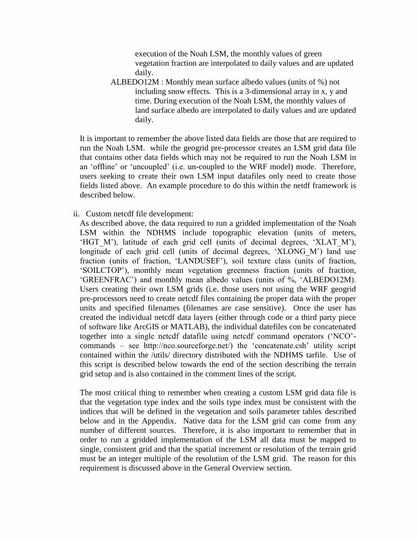
execution of the Noah LSM, the monthly values of green
vegetation fraction are interpolated to daily values and are updated
daily.
ALBEDO12M : Monthly mean surface albedo values (units of %) not
including snow effects. This is a 3-dimensional array in x, y and
time. During execution of the Noah LSM, the monthly values of
land surface albedo are interpolated to daily values and are updated
daily.
It is important to remember the above listed data fields are those that are required to
run the Noah LSM. while the geogrid pre-processor creates an LSM grid data file
that contains other data fields which may not be required to run the Noah LSM in
an „offline‟ or „uncoupled‟ (i.e. un-coupled to the WRF model) mode. Therefore,
users seeking to create their own LSM input datafiles only need to create those
fields listed above. An example procedure to do this within the netdf framework is
described below.
ii. Custom netcdf file development:
As described above, the data required to run a gridded implementation of the Noah
LSM within the NDHMS include topographic elevation (units of meters,
„HGT_M‟), latitude of each grid cell (units of decimal degrees, „XLAT_M‟),
longitude of each grid cell (units of decimal degrees, „XLONG_M‟) land use
fraction (units of fraction, „LANDUSEF‟), soil texture class (units of fraction,
„SOILCTOP‟), monthly mean vegetation greenness fraction (units of fraction,
„GREENFRAC‟) and monthly mean albedo values (units of %, „ALBEDO12M).
Users creating their own LSM grids (i.e. those users not using the WRF geogrid
pre-processors need to create netcdf files containing the proper data with the proper
units and specified filenames (filenames are case sensitive). Once the user has
created the individual netcdf data layers (either through code or a third party piece
of software like ArcGIS or MATLAB), the individual datefiles con be concatenated
together into a single netcdf datafile using netcdf command operators („NCO‟-
commands – see http://nco.sourceforge.net/) the „concatenate.csh‟ utility script
contained within the /utils/ directory distributed with the NDHMS tarfile. Use of
this script is described below towards the end of the section describing the terrain
grid setup and is also contained in the comment lines of the script.
The most critical thing to remember when creating a custom LSM grid data file is
that the vegetation type index and the soils type index must be consistent with the
indices that will be defined in the vegetation and soils parameter tables described
below and in the Appendix. Native data for the LSM grid can come from any
number of different sources. Therefore, it is also important to remember that in
order to run a gridded implementation of the LSM all data must be mapped to
single, consistent grid and that the spatial increment or resolution of the terrain grid
must be an integer multiple of the resolution of the LSM grid. The reason for this
requirement is discussed above in the General Overview section.

iii. Land surface model parameter specification:
Land surface parameters in the Noah LSM are specified in three different files:
VEGPARM.TBL : contains vegetation parameters indexed by land
use/land cover categories.
SOILPARM.TBL : contains soil physical parameters indexed by soil
textural classes.
GENPARM.TBL : contains miscellaneous model parameters that are
applied globally. Examples of these files and description of their parameters is
given in the Appendix.
c. Terrain Grid Setup
i. Overview
The high-resolution terrain routing grid specifies the data that are necessary to
route water across the landscape (via overland and saturated surbsurface flow)
and through stream channels and lakes. Options also exist to specify baseflow
values for stream channel routing based on an empirical bucket model
formulation (see Section XXXX). The data layers contained within the high-
resolution terrain grid include:
Topography (required - in units of meters)
Channel grid (required)
Flow direction (required - using the ArcGIS direction
convention)
Stream Order (required for channel routing – using the
Strahler (1952) stream order convention)
Lakes (optional)
Groundwater Basin Mask (optional)
Grid of monitoring points or stations (optional)
Grid of latitude and longitude values (often required for
proper geo-referencing of irregular gridded data in netcdf –
in units of decimal degrees)
Simple examples of each one of these grids are provided in XXXX. Data is
passed to/from the LSM grid to the terrain routing grid via a
disaggregation/aggregation scheme described in Gochis and Chen (2003). The
main requirement to enable the coarse-fine grid functionality is that terrain grid
must exactly match the extent of the LSM grid and its dimensions must be
integer multiples of the LSM grid. Given the need to interpolate, georeference
and clip grids from different sources, resolutions and spatial projections, it is
highly advantageous to use a Geographical Information System (GIS). In the
following paragraphs we provide an example procedure to create these grids,
in netcdf format using the ESRI ArcGIS system. Many other methods could
be used as well so long as care is taken to accurately map the LSM and terrain
grids to one another.
Figure 1. Example of final channel grid format with 2 lake objects present.
Note that the main channel identifier index is 0 but that this number changes at
lake/reservoir outlet to correspond with the index value of each reservoir
shown in Figure 2 below. Also, all channel grid cells underneath a lake are
assigned as -9999.
Figure 2. Example of final lake grid format with 2 lake objects present.
Figure 3. Example of final groundwater basin format with 2 groundwater
basins present.
-9999 0 -9999 -9999 -9999 0
-9999 0 -9999 -9999 0 -9999
-9999 -9999 0 -9999 -9999 -9999
-9999 -9999 0 -9999 -9999 -9999
-9999 -9999 0 -9999 1 -9999
-9999 -9999 -9999 -9999 0 -9999
-9999 -9999 -9999 -9999 -9999 -9999
-9999 -9999 -9999 -9999 -9999 -9999
-9999 -9999 -9999 2 -9999 -9999
-9999 -9999 -9999 -9999 0 -9999
-9999 -9999 -9999 -9999 0 -9999
-9999 -9999 -9999 -9999 -9999 0
-9999 -9999 -9999 -9999 -9999 0
-9999 -9999 -9999 -9999 -9999 -9999
-9999 -9999 -9999 -9999 -9999 -9999
-9999 -9999 -9999 -9999 1 -9999
-9999 -9999 -9999 -9999 1 -9999
-9999 -9999 -9999 -9999 -9999 -9999
-9999 -9999 2 -9999 -9999 -9999
-9999 -9999 2 2 -9999 -9999
-9999 -9999 2 2 -9999 -9999
-9999 -9999 -9999 -9999 -9999 -9999
-9999 -9999 -9999 -9999 -9999 -9999
-9999 -9999 -9999 -9999 -9999 -9999
-9999 -9999 -9999 -9999 -9999 -9999
-9999 -9999 -9999 -9999 -9999 -9999
-9999 -9999 -9999 -9999 -9999 -9999
-9999 -9999 -9999 -9999 -9999 -9999
-9999 -9999 -9999 -9999 1 -9999
-9999 -9999 -9999 -9999 1 -9999
-9999 -9999 -9999 -9999 -9999 -9999
-9999 -9999 2 -9999 -9999 -9999
-9999 -9999 2 2 -9999 -9999
-9999 -9999 2 2 -9999 -9999
-9999 -9999 -9999 -9999 -9999 -9999
-9999 -9999 -9999 -9999 -9999 -9999
-9999 -9999 -9999 -9999 -9999 -9999
-9999 -9999 -9999 -9999 -9999 -9999
-9999 -9999 -9999 -9999 -9999 -9999

Figure 4. Example of final forecast data point format with 4 forecast points
present.
ii. Import the LSM Grid into ArcGIS:
A step-by-step procedure to ingest and georeference the LSM geogrid file
created by the wrf pre-processors (described above) into ArcGIS is given as
follows (other methods may well be possible):
1. Using ArcGIS v9.3 or higher, import the geogrid netcdf file
using the Spatial Analyst -> Multidimension Tools ->
Create Raster Layer tool. Select the LSM terrain elevation
values on the „mass grid‟ (HGT_M) data layer from the
geogrid file for import. Specify the „x-dimension‟ to be
„east_west‟ and the „y-dimension‟ to be „north-south‟.
2. Export/Save the elevation data layer as a raster (see Figure
X for an example of how to set-up this export:
Figure X. Export layer data to raster window in ArcGIS:
3. Export the raster to an ascii data file.
4. Obtain the lat/lon value (in decimal degrees) of the center
point of the lower-left most point of the grid. This can be
done a number of ways but the simplest method is to
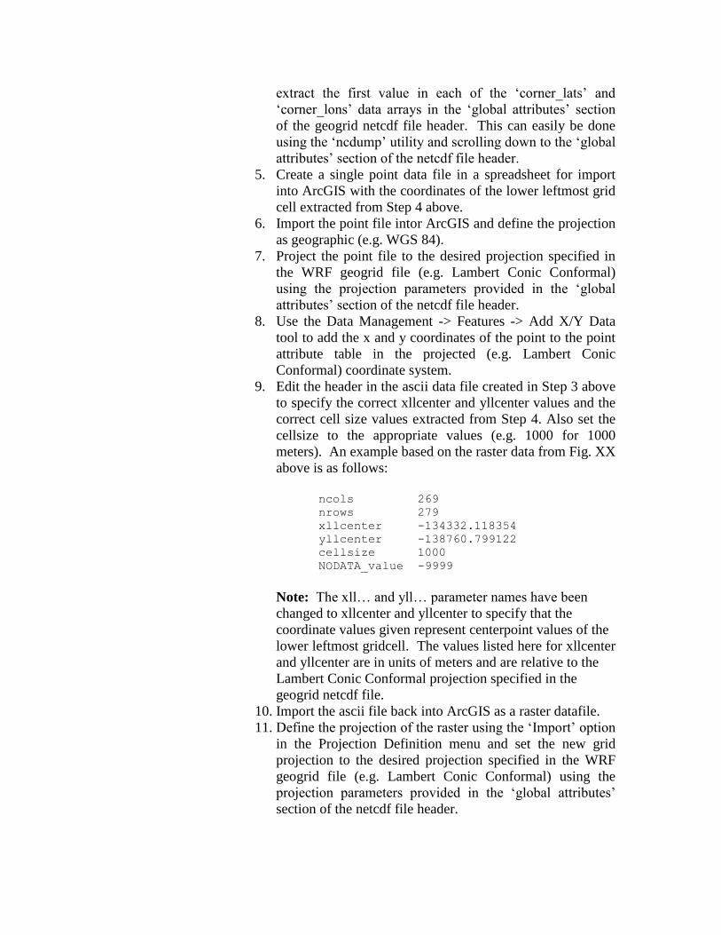
extract the first value in each of the „corner_lats‟ and
„corner_lons‟ data arrays in the „global attributes‟ section
of the geogrid netcdf file header. This can easily be done
using the „ncdump‟ utility and scrolling down to the „global
attributes‟ section of the netcdf file header.
5. Create a single point data file in a spreadsheet for import
into ArcGIS with the coordinates of the lower leftmost grid
cell extracted from Step 4 above.
6. Import the point file intor ArcGIS and define the projection
as geographic (e.g. WGS 84).
7. Project the point file to the desired projection specified in
the WRF geogrid file (e.g. Lambert Conic Conformal)
using the projection parameters provided in the „global
attributes‟ section of the netcdf file header.
8. Use the Data Management -> Features -> Add X/Y Data
tool to add the x and y coordinates of the point to the point
attribute table in the projected (e.g. Lambert Conic
Conformal) coordinate system.
9. Edit the header in the ascii data file created in Step 3 above
to specify the correct xllcenter and yllcenter values and the
correct cell size values extracted from Step 4. Also set the
cellsize to the appropriate values (e.g. 1000 for 1000
meters). An example based on the raster data from Fig. XX
above is as follows:
ncols 269
nrows 279
xllcenter -134332.118354
yllcenter -138760.799122
cellsize 1000
NODATA_value -9999
Note: The xll… and yll… parameter names have been
changed to xllcenter and yllcenter to specify that the
coordinate values given represent centerpoint values of the
lower leftmost gridcell. The values listed here for xllcenter
and yllcenter are in units of meters and are relative to the
Lambert Conic Conformal projection specified in the
geogrid netcdf file.
10. Import the ascii file back into ArcGIS as a raster datafile.
11. Define the projection of the raster using the „Import‟ option
in the Projection Definition menu and set the new grid
projection to the desired projection specified in the WRF
geogrid file (e.g. Lambert Conic Conformal) using the
projection parameters provided in the „global attributes‟
section of the netcdf file header.
12. Verify that the data is properly georeferenced by overlaying
several additional datasets of known and verified
projection.
Successful completion of these steps should create an ArcGIS raster of terrain
elevation which is properly projected according to the geographic projection
specified in the geogrid file and in the WRF/WPS pre-processing system.
iii. Processing High Resolution (~100m or less) DEM:
Once the LSM grid has been defined within ArcGIS work can proceed on
setting up the high-resolution grid. The steps to create the grids shown in Figs.
XX-XX are as follows:
1. Obtain a high-resolution digital elevation model (DEM). A near-
global (Arctic/Antarctic excepted) high resolution DEM developed
through a joint project of the World Wildlife Fund and the U.S.
Geological Survey called Hydrosheds (http://hydrosheds.cr.usgs.gov/)
provides a reasonably high quality terrain dataset which is based on
Shuttle Radar Topography Mission (SRTM) data. The resolution of
this dataset is 90m although gaps in SRTM data are filled coarser
resolution data which results in some artifacts. Additionally, the
Hydrosheds data set offers a „hydrologically-conditioned‟ DEM which
provides a more continuous flow field for use in hydrologic modeling.
(See the Hydrosheds website and documentation for full details).
The Hydrosheds data is served in 5deg by 5deg lat/lon tiles. These
tiles must be mosaicked to a single raster in ArcGIS and its spatial
projection must be defined (the initial definition of spatial project must
be that of the Hydrosheds DEM which is specified in the Hydrosheds
documentation). Following definition of spatial projection, the data
must be re-projected into the LSM grid projection which is specified in
the geogrid file. Following projection one must then clip, interpolate
and grid-match the high-resolution data to the LSM grid. Through
much trial and error we have found the following process to be the
most effective and efficient:
a) In the Spatial Analyst drop-down menu, specify the domain
„extent‟ to that of the LSM grid and define the „cell size‟
(resolution) to be the desired resolution of the high-resolution
terrain grid. For example, if the geogrid datafile has a 1km
spatial resolution a common resolution for the terrain routing
grid is 100m. Thus, 100m would be set as the cell size in the
Spatial Analyst options „cell size‟ tab.

b) Using the „Raster Calculator‟ function in the Spatial Analyst
drop-down menu, create the high resolution terrain grid using
a simple equation:
new_grid = 90m_DEM_grid
(where the 90m_DEM_grid is the mosaicked and
projected Hydrosheds DEM.)
Because the extent and cell size have already been
defined in the Spatial Analyst options sections the
„new_grid‟ will exactly match in spatial extent and grid cell
edges the LSM grid. Although other methods in ArcGIS may
be used (e.g. raster „Clip‟ function) we have found those to
be unreliable with regard to exactly matching cell size, grid
cell edges and overall extent.
2. Once the high-resolution DEM has been defined one can proceed with
deriving flow direction, channel grid and stream order grids. These
tasks exist as pre-defined functions in the Spatial Analyst->Hydrology
toolbox or as part of the ArcHydro toolbox available through
(http://www.crwr.utexs.edu/giswr/ydro/ArcHOSS/index.cfm) The
steps to derive the these fields using ArcGIS are as follows:
a) Create a „Flow Direction‟ grid using the Spatial Analyst ->
Hydrology -> FlowDirection tool. If successful, the
output grid should have integer values of 1, 2, 4, 8, 16, 32,
64 and 128 and be oriented in the following directions:
b) Create a „Flow Accumulation‟ grid using the Spatial
Analyst -> Hydrology -> FlowAccumulation
c) Define the channel grid using either the „Stream Definition‟
tool from the ArcHydro toolbox or using a logical
operation in the Spatial Analyst Raster Calculator or
Spatial Analyst Raster toolbox. Essentially, one simply
needs to specify the minimum threshold of flow
accumulation upon which a stream channel will be
defined. There is little reliable guidance for this value in a
1
2
48
16
32
64128
1
2
48
16
32
64128
„global‟ sense since climate, soils, geology, vegetation and
geomorphic processes all combine to define channel
networks. However, typical values often range between
1-10 sq. km for many temperate or humid climates.
d) (Optional for channel routing) If channel routing is to be
performed, one must specify stream order as many
channel parameters in the NDHMS are defined on the
basis of stream order. To create a grid of stream order use
the „Stream Order‟ tool within the Spatial Analyst ->
Hydrology toolbox.
e) (Optional for lake/reservoir routing) If specification of
lakes and/or reservoirs are desired one must define these
as a lake grid and, subsequently, update the channel grid
to that the channel network accurately interacts with the
specified reservoirs. The basic steps to do this include
masking out the stream channel network where reservoirs
exist (accomplished using spatial analyst logical operators
and/or the „Reclassify‟ tool) and defining the outlet of
each reservoir on the channel grid as an integer index that
matches the associated reservoir. An example of what the
lake grid and channel grid with a reservoir looks like is
shown in Figs. XX above. The steps to do this are as
follows:
i. Obtain a good quality lake coverage (e.g.
shapefile), project it to the proper projection
(e.g. Lambert Conic Conformal) and assign
a proper index for each lake ranging from 1
to n-# of lakes.
ii. Convert the lake coverage or shapefile to a
grid using the Spatial Analyst -> Feature to
Raster tool. Make sure that the proper
spatial analyst options for domain extent and
cell size have been properly set so that the
output grid will perfectly match the other
gridded data layers.
iii. Create a „reverse‟ or „negative‟ lake mask
by re-classifying all „lake grid cells‟ (e.g.
those that have data values) to „NoData‟ and
all „NoData‟ values equal to 1.
iv. In the Spatial Analyst -> Raster Calculator
tool, multiply the existing channel grid by
the „negative‟ lake mask to create a new
channel grid.

v. Convert the new channel grid file to a point
dataset using the Raster to Point tool in the
Conversions From Raster toolbox.
vi. Manually edit the output grid cell points to
have a proper lake index value associated
with the adjacent lake. Use the flow
direction grid to help trace the proper flow
path if it is not initially obvious.
vii. Convert the channel points file back to grid
using the Point to Raster tool in the
Conversions to Raster toolbox.
viii. Reclassify all no data values to -9999 and
verify that all non-outlet channel gridcells
have values of „0‟ and all channel outlet grid
cells have values according to the adjacent
lake.
f) (Optional for simple Groundwater/Baseflow
implementation, additional details are provided in Section
XXX) To permit use of the groundwater/baseflow
module in the NDHMS, one must define a groundwater
basin that receives drainage from the LSM soil column
(i.e. „recharge‟) and feeds the stream channel network (i.e.
„discharge‟). Generally, there is very little information on
the spatial extent of aquifers or their actual connectivity
with surface channel networks. Thus, we have adopted an
overly-simple approach by defining a groundwater basin
that is the same as the surface watershed defined solely by
topography. (However, other methods can be used and
users are encouraged to experiment.) To create a
watershed function one needs to define a basin outlet or
„pour point‟ in ArcGIS. Typically, this point is a gauging
station or some location where data is being or has been
collected which allows for an empirical determination of
baseflow values (see Section XXXX). Once a pour point
has been defined this point bust be „snapped‟ to the
FlowAccumulation grid defined above in c) using the
Spatial Analyst -> Hydrology toolbox. [One can create a
grid of pour points either using the „Snap Pour Points‟ tool
or using the Spatial Analyst „Feature to Raster‟ tool. In
either case care must be taken to make sure that the proper
spatial analyst options have been specified so that the grid
of pour points created perfectly matches the flow
accumulation grid.] Next the watershed can be defined
using the „Watershed‟ tool in the Spatial Analyst ->
Hydrology toolbox. The process can be repeated for
several watersheds to create multiple
groundwater/baseflow basins within the modeling domain
where each basin has an integer index value.
g) The final GIS processing step before data export to netcdf
format is to re-classify or re-assign all grids so that they
possess proper „no-data‟ values. This can be
accomplished using Spatial Analyst logical operators
and/or the „Reclassify‟ tool so that the grids EXACTLY
follow the numbering convention shown in Figures XXX-
XXX. Not following these numbering conventions will
likely result in runtime errors of the NDHMS such as a
„Segmentation Fault‟.
h) Export of the newly created high-resolution terrain fields to
netcdf is accomplished using the Spatial Analyst ->
Multidimensional Tools -> Raster to Netcdf tool. When
using this tool the proper variable names for each data
layer must be specified or else the NDHMS will not be
able to properly input the data. The correct variable
names for each data layer are as follows (these are case
sensitive):
LATITUDE
LONGITUDE
TOPGRAPHY
FLOWDIRECTION
CHANNELGRID
STREAMORDER
LAKEGRID
frxst_pts
gw_basns
Once all data layers have been properly exported to netcdf
format, the final step is to merge or „concatenate‟ all of
the individual netcdf files into a single netcdf file. There
are a variety of netcdf command operators (NCO
commands) that can be utilized to do this and we have
placed these into a simple c-shell script called
„concatenate.csh‟ which is typically distributed with the
NDHMS. Following the command line structure provided
within the script the user simply needs to issue the script
execution command followed by the list of individual
netcdf files given as command line arguments and lastly
an output file name. An example execution statement
with command line arguments is given as follows:

csh concatenate.csh file1.nc file2.nc file3.nc outfile.nc
Upon successful completion of the concatenate.csh script
the outfile.nc file will be created which contains all of the
individual data layers specified in the command line. The
most likely reason the concatenate.csh fails is because the
individual netcdf files do not all have the exact same
dimension values. This serves as one valuable check to
ensure that all of the high-resolution data layers have the
same dimensions.
Helpful notes on high-resolution grid preparation:
1. The performance and computational stability of physically-
based hydrologic simulation models is often dependent on the
characteristics and quality of the underlying terrain fields upon
which routing calculations are performed. Thus, anomalous
artifacts in DEMs can have deleterious impacts on model
stability, computational performance and/or simulation
accuracy. Thus preparation of the high-resolution terrain fields
can often be an iterative process where successive
manipulations of the DEM can be made to reduce or eliminate
large flat areas, change the density of the channel network or
add/remove lakes/reservoirs. Thus when setting up a new
domain, it is not uncommon to experiment with different
thresholds and techniques during the DEM processing stages
described above.
2. Large water bodies (the ocean, inland seas, etc) are somewhat
distinct from typical lakes and reservoirs. For most
applications, one large inland seas are treated as water sinks
and not necessarily lakes/reservoirs and the oceans are always
treated as sinks. These large water bodies are typically defined
as „water‟ grid points in the LSM. However, in the processing
of the DEM data we have adopted a convention for specifying
elevation where all ocean and large inland water bodies have
either an elevation of 0 meters or a constant elevation of the
mean lake surface elevation. Assigning these water body
elevation values will help ensure the model does not crash
since the model expects to find valid terrain elevation values
everywhere in the simulation domain (i.e. there are no „No
Data‟ or -9999 values in the topography data layer).
d. Channel Attributing
In addition to preparing the high-resolution data layers as described above, if one
desires to perform channel routing in their simulation then parameters characterizing

the channel network must be defined. These parameters are defined in a parameter
file called CHANPARM.TBL which is placed in the run directory. These parameters
are described in more detail in Section XXXX which describes the channel and lake
routing schemes but they are also briefly defined here. The values are related, or
„indexed‟, to the channel network via stream order values which are defined above.
Thus, in the present version of the model all stream pixel values of similar stream
order will have identical channel parameter values. This assumption is likely not
valid in many regions, and future versions of the model will likely include spatially-
distributed specifications of channel parameters that are assigned on the full high-
resolution terrain grids. Nevertheless, the parameters in the CHANPARM.TBL file
along with a range of possible values are defined as follows and in the Appendix:
Channel Parameters
StreamOrder
10,1, 'Bw HLINK ChSSlp MannN'
1, 5., 0.02, 1.0, 0.14
2, 10., 0.02, 0.6, 0.12
3, 20., 0.02, 0.3, 0.09
4, 30., 0.03, 0.18, 0.09
5, 40., 0.03, 0.05, 0.07
6, 60., 0.03, 0.05, 0.06
7, 60., 0.03, 0.05, 0.03
8, 60., 0.10, 0.05, 0.03
9, 60., 0.30, 0.05, 0.03
10, 60., 0.30, 0.05, 0.03
where, the first column is the Strahler stream order, „Bw‟ is the channel bottom width
(unit of meters), „HLINK‟ is the initial depth of water in the channel (unit of meters),
„ChSSlp‟ is the channel side slope (units of rise/run) and „MannN‟ is the Manning‟s
roughness coefficient for that stream order.
It is important to keep in mind that there is large uncertainty associated with these
parameters. Therefore, model calibration is almost always warranted.
Also, because fully-distributed estimates of flow depth (HLINK) are not available for
model initialization, it is almost always necessary to use a small initial value of
HLINK and let the model come to its own equilibrium (i.e. „spin-up‟) after several
hours of integration.
e. Reservoir Attributing
In addition to preparing the high-resolution data layers as described above, if one
desires to perform level-pool /lake reservoir routing in their simulation then
parameters characterizing each reservoir must be defined. These parameters are
defined in a parameter file called LAKEPARAM.TBL which is placed in the run
directory. These parameters are described in more detail in Section XXXX which
describes the channel and lake routing schemes but they are also briefly defined here.
If lake/reservoirs are not being simulated one can just assign bogus values for each

parameter in the LAKEPARAM.TBL file. Failure to put any value in the file may
result in crashing the model and receiving an I/O error message.
As described above and as shown in Fig. XX each reservoir in the lake/reservoir data
layer is assigned an integer index value ranging from 1-# of lake objects. The rest of
the lake/reservoir parameters required for level-pool reservoir routing are as follows
and in the Appendix:
lake lake index (consecutively from 1 to n # of lakes)
LkArea lake area (square meters)
LkMxH elevation of maximum lake height(in meters MSL)
WeirC weir coefficient
WeirL weir length (units of meters)
OrificC orifice coefficient
OrificeA orifice area (units of square meters)
OrificeE orifice elevation (units of meters MSL)
Lat latitude of center of mass of lake (decimal degrees)
Long latitude of center of mass of lake (decimal degrees)
Elevation mean elevation of the lake surface (units of meters
MSL)
These lake parameter values are specified for each one of the lake objects defined in
the lake grid data layer contained within the high resolution terrain grid. Typically,
several of these parameters are derived within the high-resolution terrain pre-
processing stages described above using tools such as ArcGIS. Values for the weir
and orifice coefficients and sizes can be drawn from standard engineering hydraulics
textbooks (e.g. Chow et al., 1964). Weir parameters are specified for reservoir
„overflow‟ or „spill‟ and orifice parameters are specified for design operations.
Obviously, the behavior of the reservoir to store and release water is highly dependent
on these parameters and that parameter values and reservoir operations data are often
not available.
f. Groundwater/Baseflow Basin Attributing:
In addition to preparing the high-resolution data layers as described above, if one
desires to include the representation of groundwater discharge/baseflow in their
simulation then parameters characterizing the simple baseflow bucket model must be
defined. These parameters are defined in a parameter file called
GWBUCKPARM.TBL which is placed in the run directory. These parameters are
described in more detail in Section XXXX which describes the groundwater/baseflow
scheme but they are also briefly defined here. The values in the table are related, or
„indexed‟, to each groundwater basin which is specified in the high-resolution terrain
grid described above. The parameter values in GWBUCKPARM;TBL are defined as
follows and in the Appendix:
Coeff.,Expon.,Zinit
0.4898,25.0,0.03867
0.8925,0.1394,2.0
2.1388,0.1359,1.0
0.0332,0.1615,0.5

where, „Coeff.‟ is the bucket model coefficient, „Expon.‟ is the bucket model
exponent and „Zinit‟ is the initial depth of water in the bucket model. It is important
to remember that a simple bucket model is a highly abstracted and conceptualized
representation of groundwater processes and therefore the depth of water values in the
bucket have no real physical basis. Initial values of the groundwater bucket model
parameters, including „Zinit‟ are typically derived analytically or „offline‟ from the
NDHMS and then are fine-tuned through model calibration. Full description of the
procedure to derive initial groundwater bucket model parameters are presented in
Section XXX.
Description of Output Files from the NDHMS
1. Land surface model output (YYYYMMDDHHMM.LDASOUT_DOMAINX)
When the Noah LSM is used (only option currently available), model output on
the land surface model grid is written to a multi-dimensional netcdf data file using the
file naming convention „YYYYMMDDHHMM.LDASOUT_DOMAINX‟.
where:
YYYY – year
MM – month
DD – day
HH – hour
MM – minutes
DOMAINX – the domain number that is specified in the noah_namelist input file
(also matches the domain number of the geogrid input file).
The west_east and north_south dimensions of the output file match those of the
geogrid input file. Model output is created for every model time step. However, the
length of the time dimension in each netcdf output data file can vary depending on the
value of „SPLIT_OUTPUT_COUNT‟ specified in the noah_namelist input file.
The names and definitions for each output variable in the LSM output file are
generally consistent with those output from standard Noah LSM coupled to WRF.
An example header of the netcdf output file is provided in the Appendix (see
„LDASOUT_header.txt‟). Only three new output variables are created and output on
the LSM grid as a result of the routing implementation. These variables are:
ETPNDX : Accumulated ponded water evaporation (units of mm)
INFXS : Time-step values of infiltration excess (units of mm)
SFCHEAD : Time-step values of the depth of water ponded on the soil surface of an
LSM grid cell (units of mm)
In addition to the gridded LSM output variables selected land surface variables are
output in an ASCII-formatted, basin-average, timeseries format in the „lnd_fluxes.txt‟
file. These variables can be helpful with understanding and calibrating the gross
hydrologic partitioning of land surface flux variables. One line of output is given for
each land surface model timestep. In „lnd_fluxes.txt‟ three variables are currently
output:
column 1: accumulated, basin-average, total evapotranspiration (units - mm)
column 2: accumulated, basin-average, total precipitation (units - mm)
column 3: basin-average, column-integrated soil water content (units - mm)
An example of „lnd_fluxes.txt‟ is provided in the Appendix.
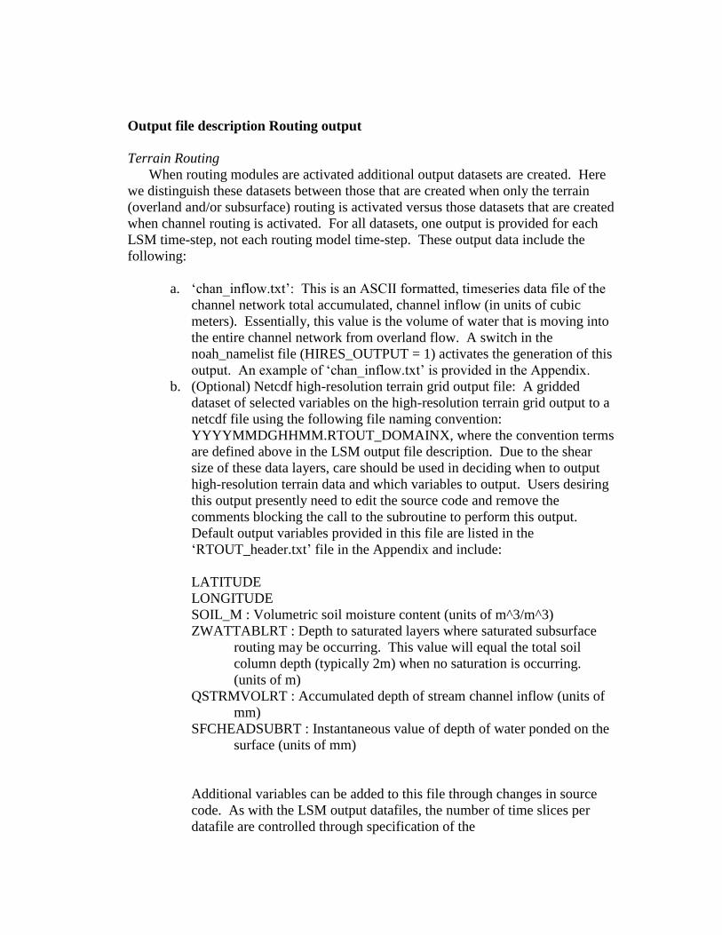
Output file description Routing output
Terrain Routing
When routing modules are activated additional output datasets are created. Here
we distinguish these datasets between those that are created when only the terrain
(overland and/or subsurface) routing is activated versus those datasets that are created
when channel routing is activated. For all datasets, one output is provided for each
LSM time-step, not each routing model time-step. These output data include the
following:
a. „chan_inflow.txt‟: This is an ASCII formatted, timeseries data file of the
channel network total accumulated, channel inflow (in units of cubic
meters). Essentially, this value is the volume of water that is moving into
the entire channel network from overland flow. A switch in the
noah_namelist file (HIRES_OUTPUT = 1) activates the generation of this
output. An example of „chan_inflow.txt‟ is provided in the Appendix.
b. (Optional) Netcdf high-resolution terrain grid output file: A gridded
dataset of selected variables on the high-resolution terrain grid output to a
netcdf file using the following file naming convention:
YYYYMMDGHHMM.RTOUT_DOMAINX, where the convention terms
are defined above in the LSM output file description. Due to the shear
size of these data layers, care should be used in deciding when to output
high-resolution terrain data and which variables to output. Users desiring
this output presently need to edit the source code and remove the
comments blocking the call to the subroutine to perform this output.
Default output variables provided in this file are listed in the
„RTOUT_header.txt‟ file in the Appendix and include:
LATITUDE
LONGITUDE
SOIL_M : Volumetric soil moisture content (units of m^3/m^3)
ZWATTABLRT : Depth to saturated layers where saturated subsurface
routing may be occurring. This value will equal the total soil
column depth (typically 2m) when no saturation is occurring.
(units of m)
QSTRMVOLRT : Accumulated depth of stream channel inflow (units of
mm)
SFCHEADSUBRT : Instantaneous value of depth of water ponded on the
surface (units of mm)
Additional variables can be added to this file through changes in source
code. As with the LSM output datafiles, the number of time slices per
datafile are controlled through specification of the

„SPLIT_OUTPUT_COUNT‟ parameter specified in the noah_namelist
input file.
Channel Routing (only output when channel routing is active)
c. „frxst_pts.txt‟: This is an ASCII-formatted data file that provides time
series of streamflow discharge at selected „forecast‟ points along the
channel network. The forecast points are specified within the „frxst_pts‟
data layer contained within the high-resolution terrain netcdf data file.
Points are listed in sequential order by station index (numbered 1 to n # of
stations) and by time. Many users will find this data file and format useful
for streamflow forecasting and model calibration. An example of
„frxst_pts.txt‟ is provided in the Appendix. The format for each data
record is as follows:
column 1 : time (in seconds) into simulation
column 2 : date and time as YYYY-MM-DD_HH:MM:SS
column 3 : station number index (numbered 0 to n-1 stations)
column 4 : station longitude (in decimal degrees)
column 5 : station latitude (in decimal degrees)
column 6 : streamflow discharge (in cubic meters per second)
column 7 : streamflow discharge (in cubic feet per second)
column 8 : flow depth/river stage (in meters above channel bottom)
d. Netcdf forecast point output :
(YYYYMMDGHHMM_CHANOBS_DOMAINX)
This is a netcdf point file which contains streamflow discharge, flow depth
(i.e. „stage‟ or „head‟), longitude, latitude, forecast point index and stream
order value for each forecast point specified in the „frxst_pts‟ data layer of
the high-resolution terrain data file. It ONLY contains data from the
forecast points and, thus, is small in file size. Users wishing to overlay
numeric streamflow values on top of other data layers such as topography
or precipitation in data visualization tools (e.g. ArcGIS, matlab, IDV, etc.)
will find this format useful. As with the LSM output datafiles, the number
of time slices per datafile are controlled through specification of the
„SPLIT_OUTPUT_COUNT‟ parameter specified in the noah_namelist
input file. An example of the netcdf data file header is provided in the
Appendix (see „CHANOBS_header.txt‟).
e. Netcdf full channel point output
(YYYYMMDGHHMM_CHRTOUT_DOMAINX)
This is a netcdf point file which is identical to the forecast point netcdf
data file except that it contains streamflow discharge, flow depth (i.e.
„stage‟ or „head‟), longitude, latitude, forecast point index and stream
order value for all channel pixels within the high-resolution terrain data
file. Because it contains data from all channel pixels within the high-

resolution terrain grid, file sizes can become quite large. Users wishing to
overlay spatially continuous numeric streamflow values on top of other
data layers such as topography or precipitation in data visualization tools
(e.g. ArcGIS, matlab, IDV, etc.) will find this format useful. As with the
LSM output datafiles, the number of time slices per datafile are controlled
through specification of the „SPLIT_OUTPUT_COUNT‟ parameter
specified in the noah_namelist input file. An example of the netcdf data
file header is provided in the Appendix (see „CHRTOUT_header.txt‟)
Lake/Reservoir Output
f. Netcdf lake point output (YYYYMMDGHHMM_LAKES_DOMAINX)
When one or more lakes/reservoirs are specified within the LAKEGRID
data layer of the high-resolution netcdf input file, a netcdf point data file is
created which contains values of several state and flux variables to/from
the lake/reservoir. An example of the header from the LAKEGRID netcdf
file is provided in the Appendix (see „LAKEOUT_header.txt‟) and some
of the most commonly used variable names are defined as follows:
ELEVATION : elevation of the lake/reservoir water surface (units of meters
above MSL)
INFLOW : total inflow to the reservoir from all channel tributaries
intersecting the lake/reservoir (units of m^3/s)
OUTFLOW : total outflow from the reservoir to a specified outlet on the
channel network (units of m^3/s)
STATION_ID : integer index of the lake numbered from 0 to n-1
lakes/reservoirs as specified in the high-resolution terrain input file.
Groundwater flux files:
When the groundwater/baseflow bucket model is activated, three
additional ASCII data files are created which help characterized the state
of (bucket depth) and fluxes (input and output) to/from the conceptual
bucket. Each datafile contains time series of values where output values
are provided for each groundwater basin. The format of each datafile is
described by the following:
g. GW_inflow.txt : Contains time-step values of drainage fluxes
from the soil column to the groundwater bucket integrated over
each groundwater basin specified in the high-resolution terrain
input file. Units of these fluxes are in meters^3.
h. GW_outflow.txt : Contains time-step values of
groundwater/baseflow bucket discharge fluxes from the bucket
to the channel network. Discharge flux values are a single
value for each groundwater basin specified in the high-

resolution terrain input file. As described in the Section
XXXX the bucket discharge values are spatially distributed
across all channel pixels contained within each groundwater
basin. Units of these fluxes are m^3/s.
i. GW_zlev.txt : Contains time-step values of the conceptual
depth of water within each bucket model. For the purposes of
mass conservation units of these fluxes are meters. However,
as mentioned previously, these values are conceptual, are
specific to the calibrated parameters of each
groundwater/baseflow bucket and do not reflect an actual depth
of water in any „natural‟ aquifer system.

REFERENCES
Chen… recent Noah doc…
Chow, V.T. and co-authors, 1964: Applied Hydrology. McGraw-Hill, Inc.
Ek…Noah doc
Gochis and Chen…
Mitchell…Noah doc…
Oleson et al…CLM doc

APPENDICES
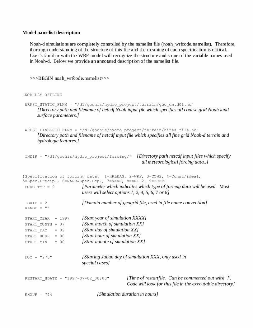
Model namelist description
Noah-d simulations are completely controlled by the namelist file (noah_wrfcode.namelist). Therefore, thorough understanding of the structure of this file and the meaning of each specification is critical.
User’s familiar with the WRF model will recognize the structure and some of the variable names used in Noah-d. Below we provide an annotated description of the namelist file.
>>>BEGIN noah_wrfcode.namelist>>>
&NOAHLSM_OFFLINE
WRFSI_STATIC_FLNM = "/d1/gochis/hydro_project/terrain/geo_em.d01.nc"
[Directory path and filename of netcdf Noah input file which specifies all coarse grid Noah land surface parameters.]
WRFSI_FINEGRID_FLNM = "/d1/gochis/hydro_project/terrain/hires_file.nc"
[Directory path and filename of netcdf input file which specifies all fine grid Noah-d terrain and hydrologic features.]
INDIR = "/d1/gochis/hydro_project/forcing/" [Directory path netcdf input files which specify
all meteorological forcing data..]
!Specification of forcing data: 1=HRLDAS, 2=WRF, 3=COWS, 4=Const/ideal,
5=Spec.Precip., 6=NARR&Spec.Pcp., 7=NARR, 8=DMIP2, 9=FRFFP
FORC_TYP = 9 [Parameter which indicates which type of forcing data will be used. Most
users will select options 1, 2, 4, 5, 6, 7 or 8]
IGRID = 2 [Domain number of geogrid file, used in file name convention] RANGE = ""
START_YEAR = 1997 [Start year of simulation XXXX]
START_MONTH = 07 [Start month of simulation XX]
START_DAY = 02 [Start day of simulation XX]
START_HOUR = 00 [Start hour of simulation XX]
START_MIN = 00 [Start minute of simulation XX]
DOY = "275" [Starting Julian day of simulation XXX, only used in
special cases]
RESTART_HDATE = "1997-07-02_00:00" [Time of restartfile. Can be commented out with ‘!’.
Code will look for this file in the executable directory]
KHOUR = 744 [Simulation duration in hours]

! KDAY = 180
! KDAY = 2
HISTORY_OUTPUT = .TRUE. [Logical switch for writing output data] !HISTORY_OUTPUT = .FALSE.
! Split history output after split_output_count output times.
SPLIT_OUTPUT_COUNT = 4 [Specify number of time steps per output file]
DT = 1800. [Model time step]
NSOIL=8 [Number of soil layer. Noah-d uses 8.]
ZSOIL8(1) = -0.10 [Thickness of each soil layer]
ZSOIL8(2) = -0.40 [.]
ZSOIL8(3) = -0.70 [.]
ZSOIL8(4) = -1.00 [.]
ZSOIL8(5) = -1.30 [.]
ZSOIL8(6) = -1.60 [.] ZSOIL8(7) = -1.90 [.]
ZSOIL8(8) = -2.00 [.]
TBOT = 288.5 [Fixed deep soil temperature] ZLVL = 2.0 [Assumed level of temperature and humidity (m)]
Z = 10.0 [Assumed level of wind speed (m)]
!Slopetyp for drainage scaling 8=no flow, 1-7 see GENPARM.TBL
SLOPETYP = 8 [Parameter for specification of bottom boundary condition. 8 = no
flow condition, other values relate to parameters specified in the GENPARM.TBL.]
!Switch for snow data assimilation: 0=no, 1=yes
SNOW_ASSIM = 0 [Switch to turn on snow updating. If set 1-‘yes’ then snow data must
be provided in forcing data files.]
!!!Optional hydrological switches for Noah-distributed
AGGFACTRT = 10 [Aggregation factor which identifies the integer multiple between the
coarse and fine grid increments.]
!-- dtrt is units of seconds
DTRT = 6 [Routing time step. Note this is a function of grid spacing due to
Courant constraints.] DXRT = 100 [Fine grid horizontal grid increment.]
SUBRTSWCRT = 1 [Switch to activate subsurface routing]

OVRTSWCRT = 1 [Switch to activate overland flow routing]
GWBASESWCRT = 0 [Switch to activate baseflow module]
CHANRTSWCRT = 0 [Switch to activate channel and reservoir routing]
!Output high-resolution routing files...0=no, 1=yes
HIRES_OUT = 1 [Switch to specify the output of data on the fine grid.
NOTE: This can generate very large files.]
!Routing Input Files... [Directory pathways and filenames for fine-grid information when
specified in flat ASCII files. Obsolete.] route_topo_f = ""
route_chan_f = ""
route_lake_f = ""
route_direction_f = ""
route_order_f = ""
route_link_f = ""
gwbasmskfil = ""
gwstrmfil = ""
! Terrain Routing Option: 1=Seepest Descent (D8) 2=CASC2D
rt_option = 1 [Switch to specify 1d or 2d routing. 1 is default.] ! Channel Routing Option: 1=Muskingam, 2=Musk.-Cunge,3=Diff.Wave
channel_option =3 [Switch to specify type of channel routing. 3 is default.]
&END
>>>END noah_wrfcode.namelist>>>

VEGPARM.TBL
Vegetation Parameters
USGS
27,1, 'ALBEDO Z0 SHDFAC NROOT RS RGL HS SNUP LAI MAXALB EMISS SFC_ROUGH'
1, .15, 1.00, .10, 1, 200., 999., 999.0, 0.04, 1.0, 40., 0.88, 0.025, 'U rban and Built-Up Land'
2, .19, .07, .80, 3, 40., 100., 36.25, 0.04, 5.68, 64., 0.92, 0.035, 'Dryland Cropland and Pasture'
3, .15, .07, .80, 3, 40., 100., 36.25, 0.04, 5.68, 64., 0.92, 0.035, 'Irrigated Crops and Pasture'
4, .17, .07, .80, 3, 40., 100., 36.25, 0.04, 4.5, 64., 0.92, 0.035, 'Mixed Dryland/Irrigated Cropland and
Pasture'
5, .19, .07, .80, 3, 40., 100., 36.25, 0.04, 4.29, 64., 0.92, 0.035, 'Cropland/Grassland Mosaic'
6, .19, .15, .80, 3, 70., 65., 44.14, 0.04, 4.0, 60., 0.93, 0.068, 'Cropland/Woodland Mosaic'
7, .19, .08, .80, 3, 40., 100., 36.35, 0.04, 2.9, 64., 0.92, 0.035, 'Grassland'
8, .25, .03, .70, 3, 300., 100., 42.00, 0.03, 3.66, 69., 0.88, 0.035, 'Shrubland'
9, .23, .05, .70, 3, 170., 100., 39.18, 0.035, 3.28, 67., 0.90, 0.035, 'Mixed Shrubland/Grassland'
10, .20, .86, .50, 3, 70., 65., 54.53, 0.04, 3.66, 45., 0.92, 0.035, 'Savanna'
11, .12, .80, .80, 4, 100., 30., 54.53, 0.08, 3.31, 58., 0.93, 0.100, 'Deciduous Broadleaf Forest'
12, .11, .85, .70, 4, 150., 30., 47.35, 0.08, 5.16, 54., 0.94, 0.100, 'Deciduous Needleleaf Forest'
13, .11, 2.65, .95, 4, 150., 30., 41.69, 0.08, 6.48, 32., 0.95, 0.100, 'Evergreen Broadleaf Forest'
14, .10, 1.09, .70, 4, 125., 30., 47.35, 0.08, 6.4, 52., 0.95, 0.100, 'Evergreen Needleleaf Forest'
15, .12, .80, .80, 4, 125., 30., 51.93, 0.08, 4.86, 53., 0.94, 0.100, 'Mixed Forest'
16, .19, .001, .00, 0, 100., 30., 51.75, 0.01, 0.01, 70., 0.98, 0.005, 'Water Bodies'
17, .12, .04, .60, 2, 40., 100., 60.00, 0.01, 5.65, 35., 0.95, 0.070, 'Herbaceous Wetland'
18, .12, .05, .60, 2, 100., 30., 51.93, 0.02, 5.8, 30., 0.95, 0.070, 'Wooded Wetland'
19, .12, .01, .01, 1, 999., 999., 999.0, 0.02, 1.0, 69., 0.85, 0.035, 'Barren or Sparsely Vegetated'
20, .16, .04, .60, 3, 150., 100., 42.00, 0.025, 3.35, 58., 0.92, 0.035, 'Herbaceous Tundra'
21, .16, .06, .60, 3, 150., 100., 42.00, 0.025, 3.35, 55., 0.93, 0.035, 'Wooded Tundra'
22, .16, .05, .60, 3, 150., 100., 42.00, 0.025, 3.35, 55., 0.92, 0.035, 'Mixed Tundra'
23, .17, .03, .30, 2, 200., 100., 42.00, 0.02, 3.35, 65., 0.85, 0.035, 'Bare Ground Tundra'
24, .70, .001, .00, 1, 999., 999., 999.0, 0.02, 0.01, 75., 0.95, 0.010, 'Snow or Ice'
25, .30, .01, .50, 1, 40., 100., 36.25, 0.02, 0.01, 69., 0.98, 0.010, 'Playa'
26, .16, .15, .00, 0, 999., 999., 999.0, 0.02, 0.01, 69., 0.97, 0.100, 'Lava'
27, .60, .01, .00, 0, 999., 999., 999.0, 0.02, 0.01, 69., 0.98, 0.010, 'White Sand'
TOPT_DATA
298.0
CMCMAX_DATA
0.5E-3
CFACTR_DATA
0.5
RSMAX_DATA
5000.0
BARE
19

where,
ALBEDO
ZO
SHDFAC
NROOT
RS
RGL
HS
SNUP
LAI
MAXALB
EMISS
SFC_ROUGH
TOPT_DATA
CMCMAX_DATA
CFACTR_DATA
RSMAX_DATA
BARE
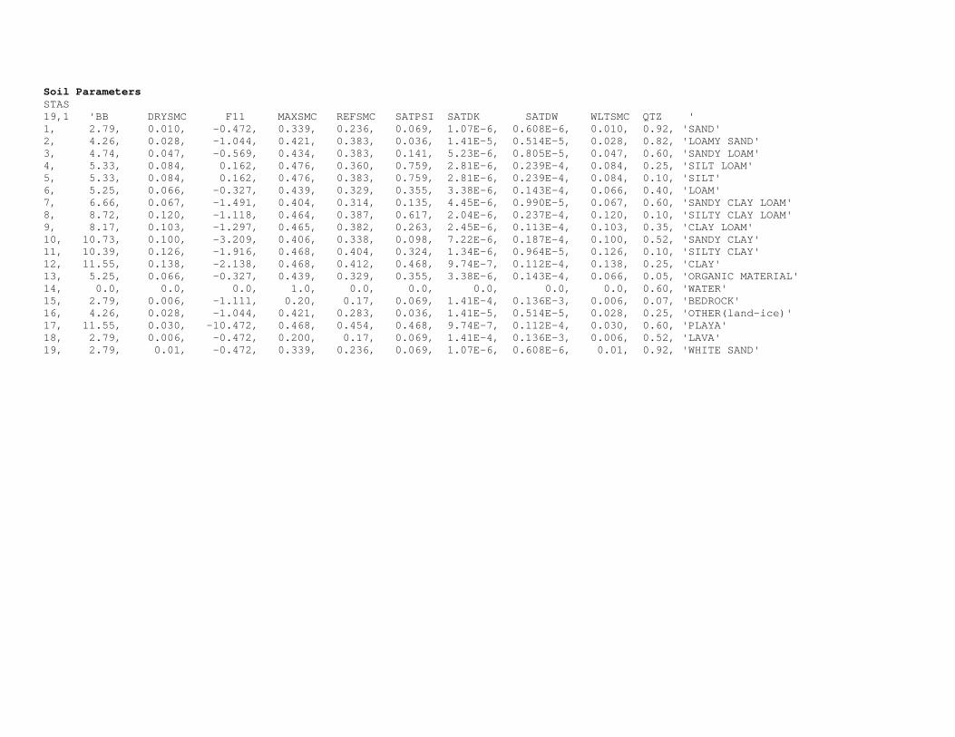
Soil Parameters STAS 19,1 'BB DRYSMC F11 MAXSMC REFSMC SATPSI SATDK SATDW WLTSMC QTZ ' 1, 2.79, 0.010, -0.472, 0.339, 0.236, 0.069, 1.07E-6, 0.608E-6, 0.010, 0.92, 'SAND' 2, 4.26, 0.028, -1.044, 0.421, 0.383, 0.036, 1.41E-5, 0.514E-5, 0.028, 0.82, 'LOAMY SAND' 3, 4.74, 0.047, -0.569, 0.434, 0.383, 0.141, 5.23E-6, 0.805E-5, 0.047, 0.60, 'SANDY LOAM' 4, 5.33, 0.084, 0.162, 0.476, 0.360, 0.759, 2.81E-6, 0.239E-4, 0.084, 0.25, 'SILT LOAM' 5, 5.33, 0.084, 0.162, 0.476, 0.383, 0.759, 2.81E-6, 0.239E-4, 0.084, 0.10, 'SILT' 6, 5.25, 0.066, -0.327, 0.439, 0.329, 0.355, 3.38E-6, 0.143E-4, 0.066, 0.40, 'LOAM' 7, 6.66, 0.067, -1.491, 0.404, 0.314, 0.135, 4.45E-6, 0.990E-5, 0.067, 0.60, 'SANDY CLAY LOAM' 8, 8.72, 0.120, -1.118, 0.464, 0.387, 0.617, 2.04E-6, 0.237E-4, 0.120, 0.10, 'SILTY CLAY LOAM' 9, 8.17, 0.103, -1.297, 0.465, 0.382, 0.263, 2.45E-6, 0.113E-4, 0.103, 0.35, 'CLAY LOAM' 10, 10.73, 0.100, -3.209, 0.406, 0.338, 0.098, 7.22E-6, 0.187E-4, 0.100, 0.52, 'SANDY CLAY' 11, 10.39, 0.126, -1.916, 0.468, 0.404, 0.324, 1.34E-6, 0.964E-5, 0.126, 0.10, 'SILTY CLAY' 12, 11.55, 0.138, -2.138, 0.468, 0.412, 0.468, 9.74E-7, 0.112E-4, 0.138, 0.25, 'CLAY' 13, 5.25, 0.066, -0.327, 0.439, 0.329, 0.355, 3.38E-6, 0.143E-4, 0.066, 0.05, 'ORGANIC MATERIAL' 14, 0.0, 0.0, 0.0, 1.0, 0.0, 0.0, 0.0, 0.0, 0.0, 0.60, 'WATER' 15, 2.79, 0.006, -1.111, 0.20, 0.17, 0.069, 1.41E-4, 0.136E-3, 0.006, 0.07, 'BEDROCK' 16, 4.26, 0.028, -1.044, 0.421, 0.283, 0.036, 1.41E-5, 0.514E-5, 0.028, 0.25, 'OTHER(land-ice)' 17, 11.55, 0.030, -10.472, 0.468, 0.454, 0.468, 9.74E-7, 0.112E-4, 0.030, 0.60, 'PLAYA' 18, 2.79, 0.006, -0.472, 0.200, 0.17, 0.069, 1.41E-4, 0.136E-3, 0.006, 0.52, 'LAVA' 19, 2.79, 0.01, -0.472, 0.339, 0.236, 0.069, 1.07E-6, 0.608E-6, 0.01, 0.92, 'WHITE SAND'
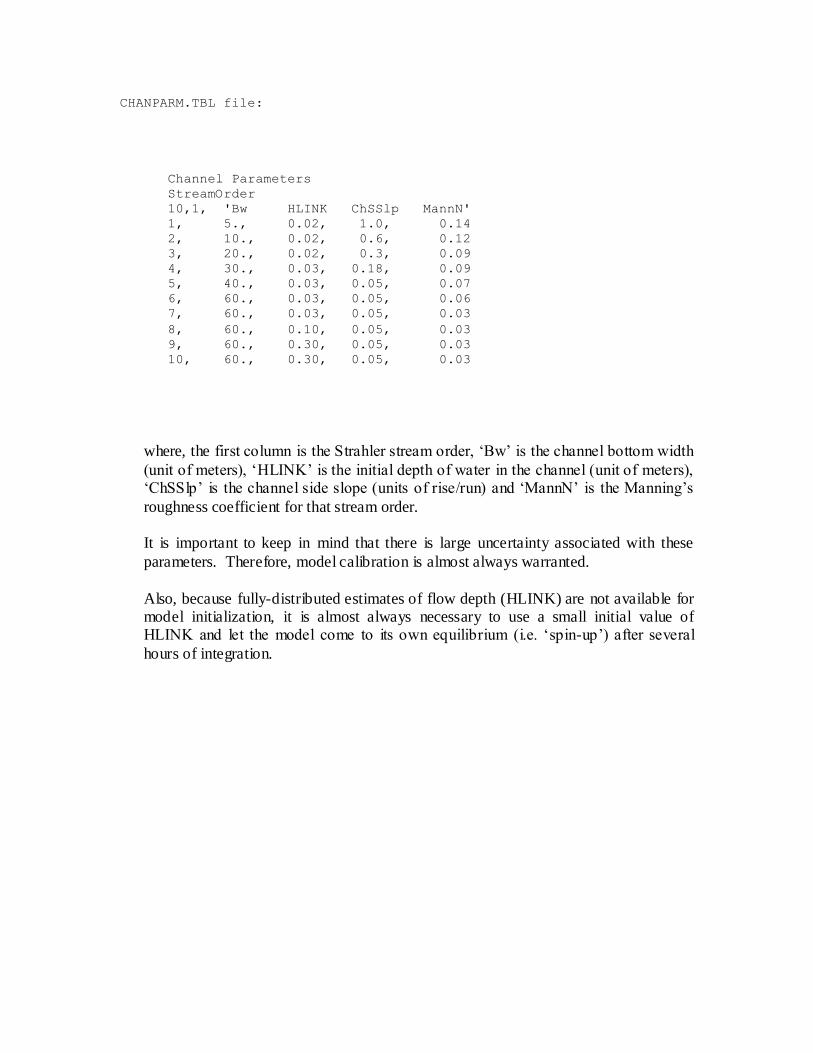
CHANPARM.TBL file:
Channel Parameters
StreamOrder
10,1, 'Bw HLINK ChSSlp MannN'
1, 5., 0.02, 1.0, 0.14
2, 10., 0.02, 0.6, 0.12
3, 20., 0.02, 0.3, 0.09
4, 30., 0.03, 0.18, 0.09
5, 40., 0.03, 0.05, 0.07
6, 60., 0.03, 0.05, 0.06
7, 60., 0.03, 0.05, 0.03
8, 60., 0.10, 0.05, 0.03
9, 60., 0.30, 0.05, 0.03
10, 60., 0.30, 0.05, 0.03
where, the first column is the Strahler stream order, ‘Bw’ is the channel bottom width
(unit of meters), ‘HLINK’ is the initial depth of water in the channel (unit of meters), ‘ChSSlp’ is the channel side slope (units of rise/run) and ‘MannN’ is the Manning’s
roughness coefficient for that stream order. It is important to keep in mind that there is large uncertainty associated with these
parameters. Therefore, model calibration is almost always warranted.
Also, because fully-distributed estimates of flow depth (HLINK) are not available for model initialization, it is almost always necessary to use a small initial value of HLINK and let the model come to its own equilibrium (i.e. ‘spin-up’) after several
hours of integration.

LAKEPARM.TBL
lake LkArea LkMxH WeirC WeirL OrificC OrificeA OrificeE lat long elevation
1 9.67 1752.1 0.4 12.1 0.1 1.0 1664.4 40.5580 -105.1586 1752.1
2 3.07 1530.8 0.4 3.8 0.1 1.0 1519.6 40.4407 -105.0586 1530.8
3 1.61 1537.7 0.4 2.0 0.1 1.0 1528.7 40.4158 -105.0903 1537.7
4 1.11 1554.6 0.4 1.4 0.1 1.0 1544.4 40.3876 -105.1441 1554.6
5 3.82 1785.1 0.4 4.8 0.1 1.0 1758.2 40.3377 -105.2196 1785.1
6 1.36 1569.5 0.4 1.7 0.1 1.0 1565.6 40.3378 -105.1278 1569.5
7 1.47 1571.1 0.4 1.8 0.1 1.0 1565.3 40.3297 -105.1167 1571.1
- this example assumes there are 7 lakes defined within the simulation domain
where, lake lake index (consecutively from 1 to n # of lakes)
LkArea lake area (square meters)
LkMxH elevation of maximum lake height(in meters MSL)
WeirC weir coefficient
WeirL weir length (units of meters)
OrificC orifice coefficient
OrificeA orifice area (units of square meters)
OrificeE orifice elevation (units of meters MSL)
Lat latitude of center of mass of lake (decimal degrees)
Long latitude of center of mass of lake (decimal degrees)
Elevation mean elevation of the lake surface (units of meters MSL)
These lake parameter values are specified for each one of the lake objects defined in the lake grid data layer contained within the high resolution terrain grid. Typically, several of these parameters are derived within the high-resolution terrain pre-processing
stages described above using tools such as ArcGIS. Values for the weir and orifice coefficients and sizes can be drawn from standard engineering hydraulics textbooks (e.g. Chow et al., 1957). Weir parameters are specified for reservoir ‘overflow’ or ‘spill’ and orifice

parameters are specified for design operations. Obviously, the behavior of the reservo ir to store and release water is highly dependent on these parameters and that parameter values and reservoir operations data are often not available.
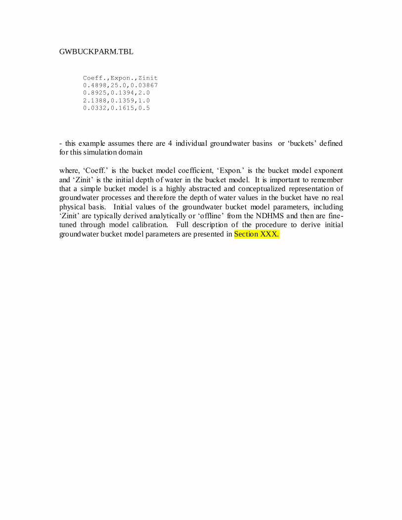
GWBUCKPARM.TBL
Coeff.,Expon.,Zinit
0.4898,25.0,0.03867
0.8925,0.1394,2.0
2.1388,0.1359,1.0
0.0332,0.1615,0.5
- this example assumes there are 4 individual groundwater basins or ‘buckets’ defined for this simulation domain
where, ‘Coeff.’ is the bucket model coefficient, ‘Expon.’ is the bucket model exponent
and ‘Zinit’ is the initial depth of water in the bucket model. It is important to remember that a simple bucket model is a highly abstracted and conceptualized representation of groundwater processes and therefore the depth of water values in the bucket have no real
physical basis. Initial values of the groundwater bucket model parameters, including ‘Zinit’ are typically derived analytically or ‘offline’ from the NDHMS and then are fine-tuned through model calibration. Full description of the procedure to derive initial
groundwater bucket model parameters are presented in Section XXX.
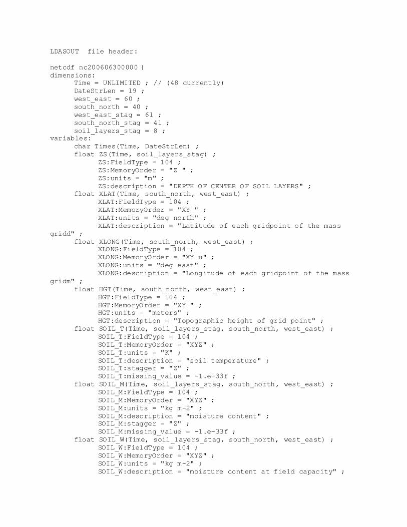
LDASOUT file header:
netcdf nc200606300000 {
dimensions:
Time = UNLIMITED ; // (48 currently)
DateStrLen = 19 ;
west_east = 60 ;
south_north = 40 ;
west_east_stag = 61 ;
south_north_stag = 41 ;
soil_layers_stag = 8 ;
variables:
char Times(Time, DateStrLen) ;
float ZS(Time, soil_layers_stag) ;
ZS:FieldType = 104 ;
ZS:MemoryOrder = "Z " ;
ZS:units = "m" ;
ZS:description = "DEPTH OF CENTER OF SOIL LAYERS" ;
float XLAT(Time, south_north, west_east) ;
XLAT:FieldType = 104 ;
XLAT:MemoryOrder = "XY " ;
XLAT:units = "deg north" ;
XLAT:description = "Latitude of each gridpoint of the mass
gridd" ;
float XLONG(Time, south_north, west_east) ;
XLONG:FieldType = 104 ;
XLONG:MemoryOrder = "XY u" ;
XLONG:units = "deg east" ;
XLONG:description = "Longitude of each gridpoint of the mass
gridm" ;
float HGT(Time, south_north, west_east) ;
HGT:FieldType = 104 ;
HGT:MemoryOrder = "XY " ;
HGT:units = "meters" ;
HGT:description = "Topographic height of grid point" ;
float SOIL_T(Time, soil_layers_stag, south_north, west_east) ;
SOIL_T:FieldType = 104 ;
SOIL_T:MemoryOrder = "XYZ" ;
SOIL_T:units = "K" ;
SOIL_T:description = "soil temperature" ;
SOIL_T:stagger = "Z" ;
SOIL_T:missing_value = -1.e+33f ;
float SOIL_M(Time, soil_layers_stag, south_north, west_east) ;
SOIL_M:FieldType = 104 ;
SOIL_M:MemoryOrder = "XYZ" ;
SOIL_M:units = "kg m-2" ;
SOIL_M:description = "moisture content" ;
SOIL_M:stagger = "Z" ;
SOIL_M:missing_value = -1.e+33f ;
float SOIL_W(Time, soil_layers_stag, south_north, west_east) ;
SOIL_W:FieldType = 104 ;
SOIL_W:MemoryOrder = "XYZ" ;
SOIL_W:units = "kg m-2" ;
SOIL_W:description = "moisture content at field capacity" ;
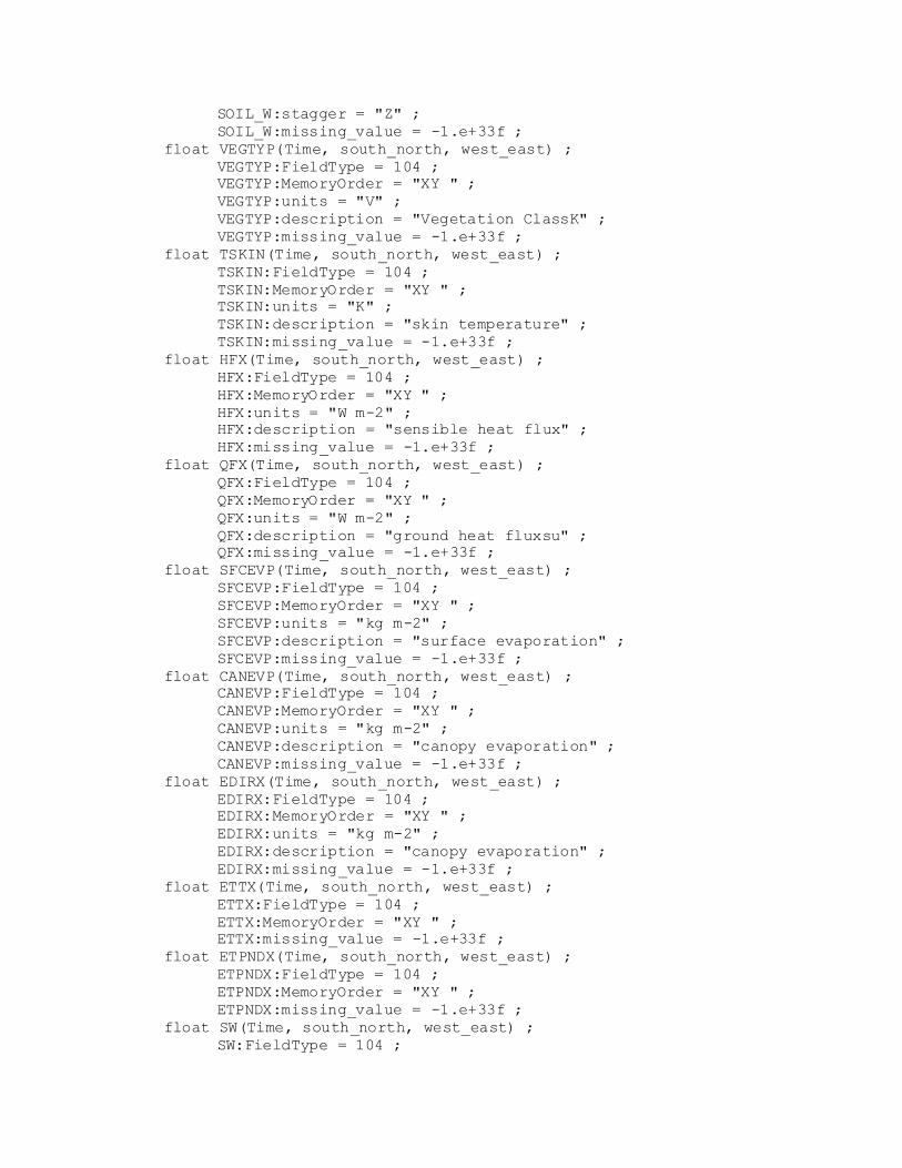
SOIL_W:stagger = "Z" ;
SOIL_W:missing_value = -1.e+33f ;
float VEGTYP(Time, south_north, west_east) ;
VEGTYP:FieldType = 104 ;
VEGTYP:MemoryOrder = "XY " ;
VEGTYP:units = "V" ;
VEGTYP:description = "Vegetation ClassK" ;
VEGTYP:missing_value = -1.e+33f ;
float TSKIN(Time, south_north, west_east) ;
TSKIN:FieldType = 104 ;
TSKIN:MemoryOrder = "XY " ;
TSKIN:units = "K" ;
TSKIN:description = "skin temperature" ;
TSKIN:missing_value = -1.e+33f ;
float HFX(Time, south_north, west_east) ;
HFX:FieldType = 104 ;
HFX:MemoryOrder = "XY " ;
HFX:units = "W m-2" ;
HFX:description = "sensible heat flux" ;
HFX:missing_value = -1.e+33f ;
float QFX(Time, south_north, west_east) ;
QFX:FieldType = 104 ;
QFX:MemoryOrder = "XY " ;
QFX:units = "W m-2" ;
QFX:description = "ground heat fluxsu" ;
QFX:missing_value = -1.e+33f ;
float SFCEVP(Time, south_north, west_east) ;
SFCEVP:FieldType = 104 ;
SFCEVP:MemoryOrder = "XY " ;
SFCEVP:units = "kg m-2" ;
SFCEVP:description = "surface evaporation" ;
SFCEVP:missing_value = -1.e+33f ;
float CANEVP(Time, south_north, west_east) ;
CANEVP:FieldType = 104 ;
CANEVP:MemoryOrder = "XY " ;
CANEVP:units = "kg m-2" ;
CANEVP:description = "canopy evaporation" ;
CANEVP:missing_value = -1.e+33f ;
float EDIRX(Time, south_north, west_east) ;
EDIRX:FieldType = 104 ;
EDIRX:MemoryOrder = "XY " ;
EDIRX:units = "kg m-2" ;
EDIRX:description = "canopy evaporation" ;
EDIRX:missing_value = -1.e+33f ;
float ETTX(Time, south_north, west_east) ;
ETTX:FieldType = 104 ;
ETTX:MemoryOrder = "XY " ;
ETTX:missing_value = -1.e+33f ;
float ETPNDX(Time, south_north, west_east) ;
ETPNDX:FieldType = 104 ;
ETPNDX:MemoryOrder = "XY " ;
ETPNDX:missing_value = -1.e+33f ;
float SW(Time, south_north, west_east) ;
SW:FieldType = 104 ;
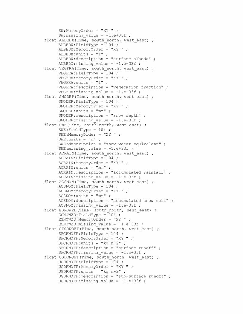
SW:MemoryOrder = "XY " ;
SW:missing_value = -1.e+33f ;
float ALBEDX(Time, south_north, west_east) ;
ALBEDX:FieldType = 104 ;
ALBEDX:MemoryOrder = "XY " ;
ALBEDX:units = "1" ;
ALBEDX:description = "surface albedo" ;
ALBEDX:missing_value = -1.e+33f ;
float VEGFRA(Time, south_north, west_east) ;
VEGFRA:FieldType = 104 ;
VEGFRA:MemoryOrder = "XY " ;
VEGFRA:units = "1" ;
VEGFRA:description = "vegetation fraction" ;
VEGFRA:missing_value = -1.e+33f ;
float SNODEP(Time, south_north, west_east) ;
SNODEP:FieldType = 104 ;
SNODEP:MemoryOrder = "XY " ;
SNODEP:units = "mm" ;
SNODEP:description = "snow depth" ;
SNODEP:missing_value = -1.e+33f ;
float SWE(Time, south_north, west_east) ;
SWE:FieldType = 104 ;
SWE:MemoryOrder = "XY " ;
SWE:units = "m" ;
SWE:description = "snow water equivalent" ;
SWE:missing_value = -1.e+33f ;
float ACRAIN(Time, south_north, west_east) ;
ACRAIN:FieldType = 104 ;
ACRAIN:MemoryOrder = "XY " ;
ACRAIN:units = "mm" ;
ACRAIN:description = "accumulated rainfall" ;
ACRAIN:missing_value = -1.e+33f ;
float ACSNOM(Time, south_north, west_east) ;
ACSNOM:FieldType = 104 ;
ACSNOM:MemoryOrder = "XY " ;
ACSNOM:units = "mm" ;
ACSNOM:description = "accumulated snow melt" ;
ACSNOM:missing_value = -1.e+33f ;
float ESNOW2D(Time, south_north, west_east) ;
ESNOW2D:FieldType = 104 ;
ESNOW2D:MemoryOrder = "XY " ;
ESNOW2D:missing_value = -1.e+33f ;
float SFCRNOFF(Time, south_north, west_east) ;
SFCRNOFF:FieldType = 104 ;
SFCRNOFF:MemoryOrder = "XY " ;
SFCRNOFF:units = "kg m-2" ;
SFCRNOFF:description = "surface runoff" ;
SFCRNOFF:missing_value = -1.e+33f ;
float UGDRNOFF(Time, south_north, west_east) ;
UGDRNOFF:FieldType = 104 ;
UGDRNOFF:MemoryOrder = "XY " ;
UGDRNOFF:units = "kg m-2" ;
UGDRNOFF:description = "sub-surface runoff" ;
UGDRNOFF:missing_value = -1.e+33f ;
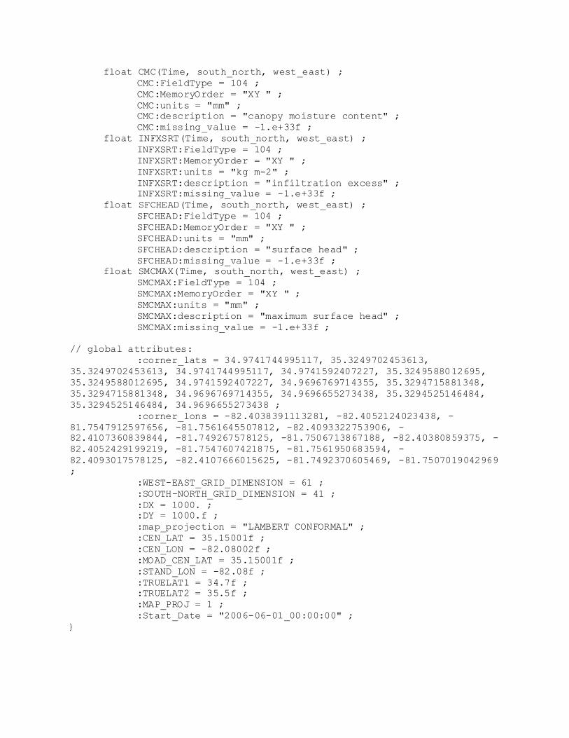
float CMC(Time, south_north, west_east) ;
CMC:FieldType = 104 ;
CMC:MemoryOrder = "XY " ;
CMC:units = "mm" ;
CMC:description = "canopy moisture content" ;
CMC:missing_value = -1.e+33f ;
float INFXSRT(Time, south_north, west_east) ;
INFXSRT:FieldType = 104 ;
INFXSRT:MemoryOrder = "XY " ;
INFXSRT:units = "kg m-2" ;
INFXSRT:description = "infiltration excess" ;
INFXSRT:missing_value = -1.e+33f ;
float SFCHEAD(Time, south_north, west_east) ;
SFCHEAD:FieldType = 104 ;
SFCHEAD:MemoryOrder = "XY " ;
SFCHEAD:units = "mm" ;
SFCHEAD:description = "surface head" ;
SFCHEAD:missing_value = -1.e+33f ;
float SMCMAX(Time, south_north, west_east) ;
SMCMAX:FieldType = 104 ;
SMCMAX:MemoryOrder = "XY " ;
SMCMAX:units = "mm" ;
SMCMAX:description = "maximum surface head" ;
SMCMAX:missing_value = -1.e+33f ;
// global attributes:
:corner_lats = 34.9741744995117, 35.3249702453613,
35.3249702453613, 34.9741744995117, 34.9741592407227, 35.3249588012695,
35.3249588012695, 34.9741592407227, 34.9696769714355, 35.3294715881348,
35.3294715881348, 34.9696769714355, 34.9696655273438, 35.3294525146484,
35.3294525146484, 34.9696655273438 ;
:corner_lons = -82.4038391113281, -82.4052124023438, -
81.7547912597656, -81.7561645507812, -82.4093322753906, -
82.4107360839844, -81.749267578125, -81.7506713867188, -82.40380859375, -
82.4052429199219, -81.7547607421875, -81.7561950683594, -
82.4093017578125, -82.4107666015625, -81.7492370605469, -81.7507019042969
;
:WEST-EAST_GRID_DIMENSION = 61 ;
:SOUTH-NORTH_GRID_DIMENSION = 41 ;
:DX = 1000. ;
:DY = 1000.f ;
:map_projection = "LAMBERT CONFORMAL" ;
:CEN_LAT = 35.15001f ;
:CEN_LON = -82.08002f ;
:MOAD_CEN_LAT = 35.15001f ;
:STAND_LON = -82.08f ;
:TRUELAT1 = 34.7f ;
:TRUELAT2 = 35.5f ;
:MAP_PROJ = 1 ;
:Start_Date = "2006-06-01_00:00:00" ;
}
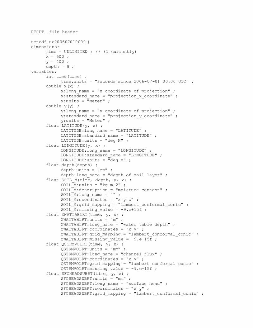
RTOUT file header
netcdf nc200607010000 {
dimensions:
time = UNLIMITED ; // (1 currently)
x = 600 ;
y = 400 ;
depth = 8 ;
variables:
int time(time) ;
time:units = "seconds since 2006-07-01 00:00 UTC" ;
double x(x) ;
x:long_name = "x coordinate of projection" ;
x:standard_name = "projection_x_coordinate" ;
x:units = "Meter" ;
double y(y) ;
y:long_name = "y coordinate of projection" ;
y:standard_name = "projection_y_coordinate" ;
y:units = "Meter" ;
float LATITUDE(y, x) ;
LATITUDE:long_name = "LATITUDE" ;
LATITUDE:standard_name = "LATITUDE" ;
LATITUDE:units = "deg N" ;
float LONGITUDE(y, x) ;
LONGITUDE:long_name = "LONGITUDE" ;
LONGITUDE:standard_name = "LONGITUDE" ;
LONGITUDE:units = "deg e" ;
float depth(depth) ;
depth:units = "cm" ;
depth:long_name = "depth of soil layer" ;
float SOIL_M(time, depth, y, x) ;
SOIL_M:units = "kg m-2" ;
SOIL_M:description = "moisture content" ;
SOIL_M:long_name = "" ;
SOIL_M:coordinates = "x y z" ;
SOIL_M:grid_mapping = "lambert_conformal_conic" ;
SOIL_M:missing_value = -9.e+15f ;
float ZWATTABLRT(time, y, x) ;
ZWATTABLRT:units = "m" ;
ZWATTABLRT:long_name = "water table depth" ;
ZWATTABLRT:coordinates = "x y" ;
ZWATTABLRT:grid_mapping = "lambert_conformal_conic" ;
ZWATTABLRT:missing_value = -9.e+15f ;
float QSTRMVOLRT(time, y, x) ;
QSTRMVOLRT:units = "mm" ;
QSTRMVOLRT:long_name = "channel flux" ;
QSTRMVOLRT:coordinates = "x y" ;
QSTRMVOLRT:grid_mapping = "lambert_conformal_conic" ;
QSTRMVOLRT:missing_value = -9.e+15f ;
float SFCHEADSUBRT(time, y, x) ;
SFCHEADSUBRT:units = "mm" ;
SFCHEADSUBRT:long_name = "surface head" ;
SFCHEADSUBRT:coordinates = "x y" ;
SFCHEADSUBRT:grid_mapping = "lambert_conformal_conic" ;

SFCHEADSUBRT:missing_value = -9.e+15f ;
int lambert_conformal_conic ;
lambert_conformal_conic:grid_mapping_name =
"lambert_conformal_conic" ;
lambert_conformal_conic:longitude_of_central_meridian = -
82.08f ;
lambert_conformal_conic:latitude_of_projection_origin =
35.15f ;
lambert_conformal_conic:false_easting = 0.f ;
lambert_conformal_conic:false_northing = 0.f ;
lambert_conformal_conic:standard_parallel = 34.7f, 35.5f ;
// global attributes:
:missing_value = -9.e+15f ;
:Conventions = "CF-1.0" ;
:time_coverage_start = "2006-06-01_00:00:00" ;
:output_decimation_factor = 1 ;
:time_coverage_end = "2006-07-01_00:00:00" ;
}
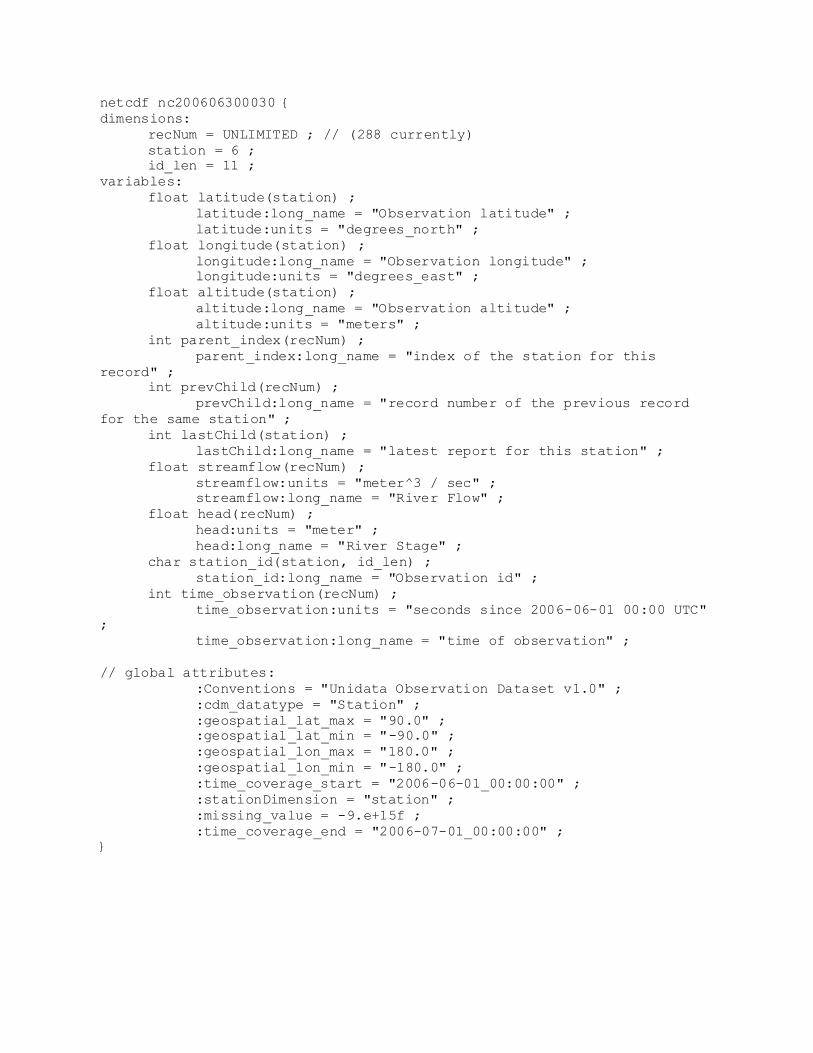
netcdf nc200606300030 {
dimensions:
recNum = UNLIMITED ; // (288 currently)
station = 6 ;
id_len = 11 ;
variables:
float latitude(station) ;
latitude:long_name = "Observation latitude" ;
latitude:units = "degrees_north" ;
float longitude(station) ;
longitude:long_name = "Observation longitude" ;
longitude:units = "degrees_east" ;
float altitude(station) ;
altitude:long_name = "Observation altitude" ;
altitude:units = "meters" ;
int parent_index(recNum) ;
parent_index:long_name = "index of the station for this
record" ;
int prevChild(recNum) ;
prevChild:long_name = "record number of the previous record
for the same station" ;
int lastChild(station) ;
lastChild:long_name = "latest report for this station" ;
float streamflow(recNum) ;
streamflow:units = "meter^3 / sec" ;
streamflow:long_name = "River Flow" ;
float head(recNum) ;
head:units = "meter" ;
head:long_name = "River Stage" ;
char station_id(station, id_len) ;
station_id:long_name = "Observation id" ;
int time_observation(recNum) ;
time_observation:units = "seconds since 2006-06-01 00:00 UTC"
;
time_observation:long_name = "time of observation" ;
// global attributes:
:Conventions = "Unidata Observation Dataset v1.0" ;
:cdm_datatype = "Station" ;
:geospatial_lat_max = "90.0" ;
:geospatial_lat_min = "-90.0" ;
:geospatial_lon_max = "180.0" ;
:geospatial_lon_min = "-180.0" ;
:time_coverage_start = "2006-06-01_00:00:00" ;
:stationDimension = "station" ;
:missing_value = -9.e+15f ;
:time_coverage_end = "2006-07-01_00:00:00" ;
}
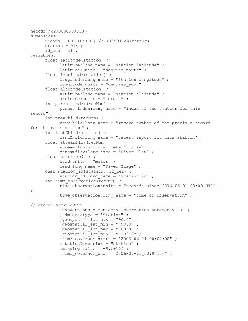
netcdf nc200606300030 {
dimensions:
recNum = UNLIMITED ; // (45504 currently)
station = 948 ;
id_len = 11 ;
variables:
float latitude(station) ;
latitude:long_name = "Station latitude" ;
latitude:units = "degrees_north" ;
float longitude(station) ;
longitude:long_name = "Station longitude" ;
longitude:units = "degrees_east" ;
float altitude(station) ;
altitude:long_name = "Station altitude" ;
altitude:units = "meters" ;
int parent_index(recNum) ;
parent_index:long_name = "index of the station for this
record" ;
int prevChild(recNum) ;
prevChild:long_name = "record number of the previous record
for the same station" ;
int lastChild(station) ;
lastChild:long_name = "latest report for this station" ;
float streamflow(recNum) ;
streamflow:units = "meter^3 / sec" ;
streamflow:long_name = "River Flow" ;
float head(recNum) ;
head:units = "meter" ;
head:long_name = "River Stage" ;
char station_id(station, id_len) ;
station_id:long_name = "Station id" ;
int time_observation(recNum) ;
time_observation:units = "seconds since 2006-06-01 00:00 UTC"
;
time_observation:long_name = "time of observation" ;
// global attributes:
:Conventions = "Unidata Observation Dataset v1.0" ;
:cdm_datatype = "Station" ;
:geospatial_lat_max = "90.0" ;
:geospatial_lat_min = "-90.0" ;
:geospatial_lon_max = "180.0" ;
:geospatial_lon_min = "-180.0" ;
:time_coverage_start = "2006-06-01_00:00:00" ;
:stationDimension = "station" ;
:missing_value = -9.e+15f ;
:time_coverage_end = "2006-07-01_00:00:00" ;
}

LAKEOUT file header
netcdf nc200606300030 {
dimensions:
recNum = UNLIMITED ; // (96 currently)
station = 2 ;
id_len = 6 ;
variables:
float latitude(station) ;
latitude:long_name = "Lake latitude" ;
latitude:units = "degrees_north" ;
float longitude(station) ;
longitude:long_name = "Lake longitude" ;
longitude:units = "degrees_east" ;
float altitude(station) ;
altitude:long_name = "Lake altitude" ;
altitude:units = "meters" ;
int parent_index(recNum) ;
parent_index:long_name = "index of the lake for this record"
;
int prevChild(recNum) ;
prevChild:long_name = "record number of the previous record
for the same lake" ;
int lastChild(station) ;
lastChild:long_name = "latest report for this lake" ;
float elevation(recNum) ;
elevation:units = "meters" ;
elevation:long_name = "Lake Elevation" ;
float inflow(recNum) ;
inflow:units = "meter^3 / sec" ;
float outflow(recNum) ;
outflow:units = "meter^3 / sec" ;
char station_id(station, id_len) ;
station_id:long_name = "Station id" ;
int time_observation(recNum) ;
time_observation:units = "seconds since 2006-06-01 00:00 UTC"
;
time_observation:long_name = "time of observation" ;
// global attributes:
:Conventions = "Unidata Observation Dataset v1.0" ;
:cdm_datatype = "Station" ;
:geospatial_lat_max = "90.0" ;
:geospatial_lat_min = "-90.0" ;
:geospatial_lon_max = "180.0" ;
:geospatial_lon_min = "-180.0" ;
:time_coverage_start = "2006-06-01_00:00:00" ;
:stationDimension = "station" ;
:missing_value = -9.e+15f ;
:time_coverage_end = "2006-07-01_00:00:00" ;
}
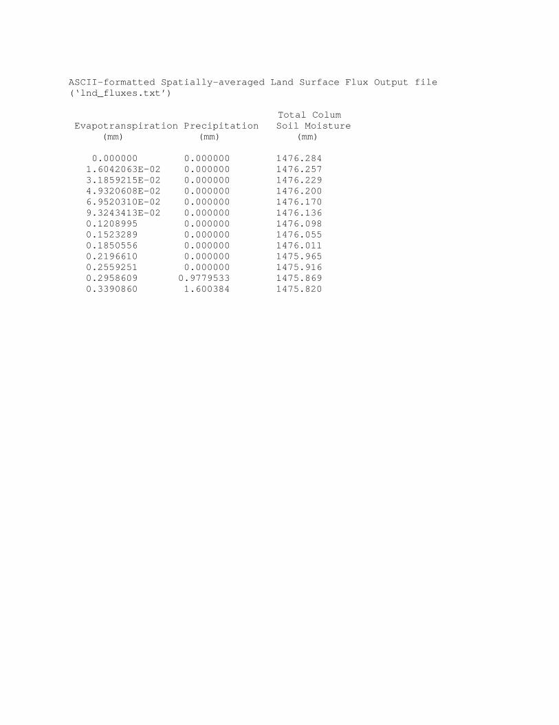
ASCII-formatted Spatially-averaged Land Surface Flux Output file (‘lnd_fluxes.txt’) Total Colum Evapotranspiration Precipitation Soil Moisture (mm) (mm) (mm) 0.000000 0.000000 1476.284 1.6042063E-02 0.000000 1476.257 3.1859215E-02 0.000000 1476.229 4.9320608E-02 0.000000 1476.200 6.9520310E-02 0.000000 1476.170 9.3243413E-02 0.000000 1476.136 0.1208995 0.000000 1476.098 0.1523289 0.000000 1476.055 0.1850556 0.000000 1476.011 0.2196610 0.000000 1475.965 0.2559251 0.000000 1475.916 0.2958609 0.9779533 1475.869 0.3390860 1.600384 1475.820
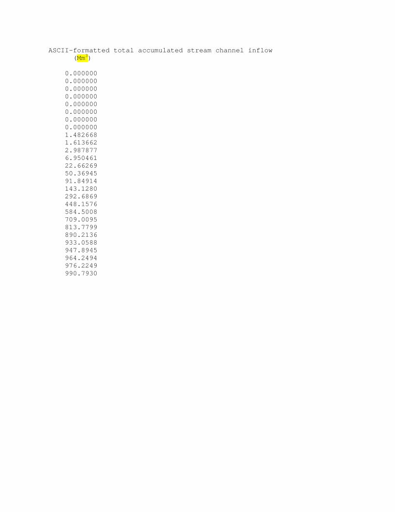
ASCII-formatted total accumulated stream channel inflow (Mm3) 0.000000 0.000000 0.000000 0.000000 0.000000 0.000000 0.000000 0.000000 1.482668 1.613662 2.987877 6.950461 22.66269 50.36945 91.84914 143.1280 292.6869 448.1576 584.5008 709.0095 813.7799 890.2136 933.0588 947.8945 964.2494 976.2249 990.7930

ASCII Forecast/Observation Point Output File (‘frxst_pts_out.txt’) Flowrate Flowrate Head Time (sec) Date Stn. Lon. Lat. cms cfs m 3600 2005-01-01_01:00:00 0 -94.37383 36.58603 16.038 566.378 1.236 3600 2005-01-01_01:00:00 1 -94.44971 36.59901 20.239 714.749 1.281 3600 2005-01-01_01:00:00 2 -94.18576 36.62368 11.989 423.380 1.182 3600 2005-01-01_01:00:00 3 -94.58810 36.63018 76.155 2689.410 0.983 7200 2005-01-01_02:00:00 0 -94.37383 36.58603 15.794 557.772 1.226 7200 2005-01-01_02:00:00 1 -94.44971 36.59901 20.030 707.355 1.276 7200 2005-01-01_02:00:00 2 -94.18576 36.62368 11.770 415.665 1.172 7200 2005-01-01_02:00:00 3 -94.58810 36.63018 75.694 2673.123 0.980 10800 2005-01-01_03:00:00 0 -94.37383 36.58603 15.530 548.436 1.214 10800 2005-01-01_03:00:00 1 -94.44971 36.59901 19.877 701.947 1.271 10800 2005-01-01_03:00:00 2 -94.18576 36.62368 11.566 408.458 1.161 10800 2005-01-01_03:00:00 3 -94.58810 36.63018 75.250 2657.438 0.978 14400 2005-01-01_04:00:00 0 -94.37383 36.58603 15.213 537.264 1.201 14400 2005-01-01_04:00:00 1 -94.44971 36.59901 19.687 695.234 1.266 14400 2005-01-01_04:00:00 2 -94.18576 36.62368 11.344 400.615 1.149 14400 2005-01-01_04:00:00 3 -94.58810 36.63018 74.722 2638.802 0.974

ASCII-formatted total accumulated inflow into the groundwater bucket(s): (m^3) 11427.19 11439.82 11452.33 11464.78 11477.20 11489.57 11501.90 11514.20 11526.46 11538.66 11550.76 11562.80 11574.76 11586.68 11598.56

ASCII-formatted outflow rate from the groundwater bucket(s): (m^3/s) 0.4911679 0.4923286 0.4934930 0.4946613 0.4958332 0.4970090 0.4981885 0.4993718 0.5005589 0.5017497 0.5029444 0.5041428 0.5053451 0.5065511 0.5077611 0.5089747 0.5101923 0.5114136 0.5126388