near-infrared spectral monitoring of triton with irtf/spex...
TRANSCRIPT
Near-infrared spectral monitoring of Triton with IRTF/SpeX I:
Establishing a baseline for rotational variability
W.M. Grundy1
Lowell Observatory, 1400 W. Mars Hill Rd., Flagstaff AZ 86001
L.A. Young1
Southwest Research Institute, 1050 Walnut St., Boulder CO 80302
1Visiting observer at the Infrared Telescope Facility, which is operated by the University of
Hawaii under contract from the National Aeronautics and Space Administration
— Submitted to Icarus —
Received 2004/04/07 ; accepted
Primary contact: Will Grundy
E-mail: [email protected]
Voice: 928-774-3358
Fax: 928-774-6296
Running head: Triton monitoring
Manuscript pages: 37
Figures: 10
Tables: 1
– 2 –
ABSTRACT
We present eight new 0.8 to 2.4 µm spectral observations of Neptune’s satellite
Triton, obtained at IRTF/SpeX during 2002 July 15–22 UT. Our objective was
to determine how Triton’s near-infrared spectrum varies as Triton rotates, and to
establish an accurate baseline for comparison with past and future observations.
The most striking spectral change detected was in Triton’s nitrogen ice absorption
band at 2.15 µm; its strength varies by about a factor of two as Triton rotates.
Maximum N2 absorption approximately coincides with Triton’s Neptune-facing
hemisphere, which is also the longitude where the polar cap extends nearest
Triton’s equator. More subtle rotational variations are reported for Triton’s CH4
and H2O ice absorption bands. Unlike the other ices, Triton’s CO2 ice absorption
bands remain nearly constant as Triton rotates. Triton’s H2O ice is shown to be
crystalline, rather than amorphous. Triton’s N2 ice is confirmed to be the warmer,
hexagonal, β N2 phase, and its CH4 is confirmed to be highly diluted in N2 ice.
Subject headings: Ices; satellite surfaces; satellites of Neptune; infrared
observations; volatile transport
1. Introduction
Neptune’s moon, Triton, experiences complex seasonal variations in its subsolar
latitude due to the combination of Neptune’s obliquity and Triton’s inclined orbit (Trafton
1984; Forget et al. 2000). These variations are expected to drive complex seasonal changes
in Triton’s surface and atmosphere. Because Triton’s N2-dominated atmosphere is in
vapor-pressure equilibrium with its N2 surface ice, small changes in ice temperature cause
extreme changes in surface pressure (Brown and Ziegler 1980). As changes in subsolar
– 3 –
latitude alter insolation patterns, Triton’s surface pressure is expected to vary by one to
two orders of magnitude (Trafton 1984; Stansberry et al. 1990; Hansen and Paige 1992;
Spencer and Moore 1992; Forget et al. 2000), with corresponding seasonal changes in the
distributions of volatile N2, CO, and CH4 ices on Triton’s surface.
Observers have reported evidence of change on Triton on both long and short time
scales, from stellar occultations, and from spectroscopy and photometry at UV, visible,
and IR wavelengths. Stellar occultations in 1993, 1995, and 1997 indicate that Triton’s
atmospheric pressure has increased since the 1989 Voyager encounter, with the surface
pressure rising from 14 to 19 µbar (Elliot et al. 1998, 2000a,b). Visible photometry spanning
1952 to 1990 shows a long-term blue-ing trend in Triton’s U −B and B − V colors (Buratti
et al. 1994). Superimposed on this trend are occasional reddening episodes with time scales
of less than a year (Buratti et al. 1999; Hicks and Buratti 2004); a similar reddening was
also seen between 1977 and 1989 (see Brown et al. 1995, for a review). These reddenings
decrease the flux at 0.35 µm by nearly a factor of two relative to the flux at 0.6 µm. In
the mid-UV (0.279-0.311 µm) Triton brightened by roughly 27% between 1993 and 1999
(Young and Stern 2001). These interannual changes in UV and visible albedos and colors
are much larger than variations seen with rotational phase; Triton’s lightcurve amplitude
at 0.27 µm is 8%, and only 5% at 0.35 µm (Hillier et al. 1991; Young and Stern 2001),
so the observed changes reflect secular, rather than rotational variations. Similarly, the
occultation results most likely imply global-scale changes (Elliot et al. 2000b).
Interpretations of these changes have invoked effects including volatile transport (e.g.,
Trafton 1984; Spencer 1990; Stansberry et al. 1990; Hansen and Paige 1992; Grundy
and Stansberry 2000), photochemical processing of atmospheric gases and surface ices
(e.g., Delitsky and Thompson 1987; Johnson 1989; McDonald et al. 1994; Salama 1998;
Strazzulla 1998; Hudson and Moore 2001; Moore and Hudson 2003), changes in ice particle
– 4 –
size and porosity due to annealing or sintering (e.g., Clark et al. 1983; Eluszkiewicz 1991;
Eluszkiewicz et al. 1998; Eluszkiewicz and Moncet 2003), and atmospheric deposition,
mechanical under-turning, and thermally-induced submersion, of thin (∼100 micron) layers
on Triton’s surface (as discussed by Young and Stern 2001).
To test the theoretical models and to make sense of the clues from occultation, UV, and
visible data, we want to monitor changes in the composition, mixing state, temperature,
and grain sizes of the ices on Triton’s surface. To date, the near-infrared is the only
spectral region to reveal this information (e.g., Cruikshank et al. 1993; Quirico et al.
1999; Cruikshank et al. 2000). Historical evidence for spectral changes at near-infrared
wavelengths is ambiguous. As reviewed by Brown et al. (1995), Triton’s CH4 absorption
bands were stronger in 1980 (on Triton’s leading hemisphere) than in 1981 (on Triton’s
trailing hemisphere). It is unclear whether these changes are related to spatial or temporal
variability. Furthermore, the earlier datasets have very low signal-to-noise and spectral
resolution (λ/∆λ ∼20 in 1980) compared with what can be routinely obtained at present.
To improve temporal sampling of Triton’s near-infrared spectrum, in 2002 we began
a new program of high-quality spectroscopic monitoring using consistent data acquisition
methods, with observations roughly once a month during each Triton apparition. In light
of possible longitudinal variation in CH4 band strength (e.g., Cruikshank and Apt 1984;
Cruikshank et al. 1988), we began this program by observing Triton on eight consecutive
nights. These initial observations, the subject of this paper, serve two purposes. First, being
spaced at roughly 61◦ subsolar longitude intervals, these observations provide information
on the longitudinal distribution of ices on Triton’s surface. Second, they create a fiducial
data set against which to compare past and future observations by ourselves and others.
– 5 –
2. Observations and Reduction
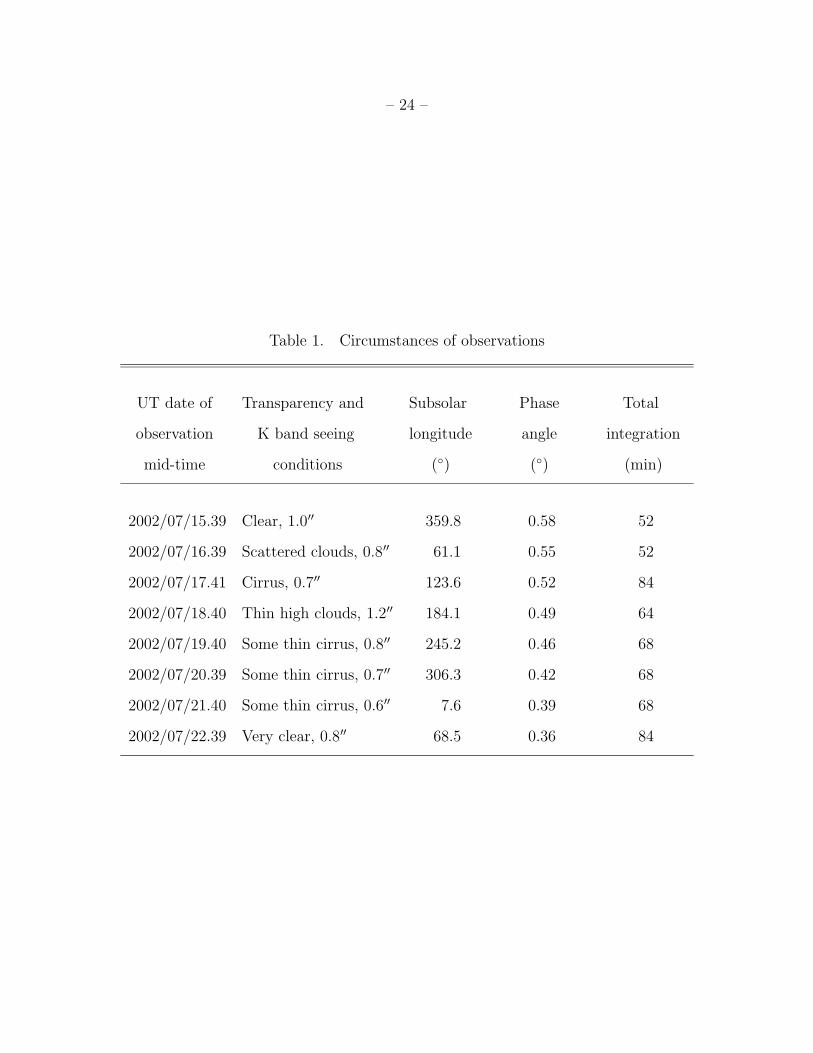
We obtained rotationally resolved infrared spectroscopy of Triton over eight consecutive
nights (2002 July 15–22 UT) at NASA’s Infrared Telescope Facility (IRTF) on Mauna Kea
as tabulated in Table 1. Triton’s rotational period and orbital period about Neptune are
both 5.877 days, so 8 nights provided some protection against weather loss and also enabled
direct comparison of similar rotational phases at the beginning and end of our run. Weather
was acceptable for spectroscopy on all eight nights. We used the short cross-dispersed mode
of the SpeX spectrograph (Rayner et al. 1998, 2003), covering the 0.8 to 2.4 µm wavelength
range with five spectral orders, recorded simultaneously on a 1024×1024 InSb array.
EDITOR: Please place TABLE 1 near here.
To minimize spurious spectral slopes which can arise from differential atmospheric
refraction, we used an image rotator to keep SpeX’s 0.3 arcsec slit oriented on the
sky-plane as close to the parallactic angle as possible. The parallactic angle is the sky-plane
projection of the plane defined by observer-object and observer-zenith vectors, and gives the
orientation on the sky-plane of light dispersion due to differential atmospheric refraction. It
is desirable to maintain alignment of the slit with the parallactic angle, especially at high
airmasses, but the necessity of keeping Neptune well away from the slit interfered with
that goal. Near transit, when the airmass was low (∼1.3) and the parallactic angle rotated
rapidly, we kept the slit within 60◦ of the parallactic angle. During the more critical higher
airmass observations (nightly maximum airmass was ∼1.85) we kept the slit within 15◦ of
the parallactic angle, resulting in a maximum cross-slit dispersion between 0.8 and 2.4 µm
of less than 0.2 arcsec, which compares favorably with the 0.6 arcsec width of the best K
band seeing disk encountered during the run. We could not find evidence in our Triton data
for the spurious spectral slopes characteristic of differential refraction problems.
– 6 –
Spectral extraction was accomplished using the Horne (1986) optimal extraction
algorithm as implemented by M.W. Buie et al. at Lowell Observatory (e.g., Buie and
Grundy 2000; Grundy and Buie 2001; Grundy et al. 2002a).
We alternated observations of Triton with those of nearby reference star HD 202282,
cataloged as spectral class G3V (Houk and Smith-Moore 1988), in addition to more distant,
well-known solar analogs 16 Cyg B, BS 5968, BS 6060, and SA 112-1333. Observations of
the latter four stars were used to determine that HD 202282 is also an excellent solar analog
in this spectral range. From the suite of solar analog observations obtained each night we
computed telluric extinction, enabling us to correct all star and Triton observations to a
common airmass. We then divided the airmass-corrected Triton spectra by the mean of
the airmass-corrected solar analog spectra. Because the flux from Triton is entirely due
to reflected sunlight over the observed wavelength range, this operation produced spectra
proportional to Triton’s disk-integrated albedo, as well as eliminating most instrumental
and telluric spectral features. Residual telluric features do remain near 1.4 and 1.9 µm,
where strong and narrow telluric H2O vapor absorptions make sky transparency especially
variable in time. Final, normalized albedo spectra of Triton from the eight nights are shown
in Fig. 1.
EDITOR: Please place FIGURE 1 near here.
Wavelength calibration was derived from telluric sky emission lines extracted from
the Triton frames and from separate observations of SpeX’s internal integrating sphere,
illuminated by a low-pressure argon arc lamp. Profiles of these line sources were well
approximated by Gaussians having full width at half maximum (FWHM) of ∼2.5
pixels, implying resolving power (λ/∆λ) between 1600 and 1700 over our spectral range.
Wavelength uncertainty, primarily due to flexure within SpeX, is approximately one pixel.
– 7 –
With Triton and reference star seeing disks uniformly wider than the slit, these filled slit
resolutions and wavelength uncertainties apply to all of our observations.
It is not possible to quote absolute albedos from narrow-slit spectra alone, since variable
slit losses (e.g., due to tracking or changes in seeing) undermine the photometric fidelity of
comparisons between targets and standards. For the night of 2002 July 21, M. Connelly
kindly took JHK photometry of Triton for us with the University of Hawaii’s 2.2 m telescope
at Mauna Kea with the QUIRC IR array (Hodapp et al. 1996). The standard star was
FS137 (from the UKIRT extended faint standards list, Casali and Hawarden 1992), and we
corrected for the ∼0.5 airmass difference using the mean Mauna Kea extinction values of
Krisciunas et al. (1987). Under these assumptions, Triton’s average geometric albedos were
0.964, 0.811, and 0.603 through the J, H, and K filters, respectively, on this night, consistent
(to the 10% quality of our photometry) with the IR colors tabulated in Cox (2000).
3. Analysis and Discussion
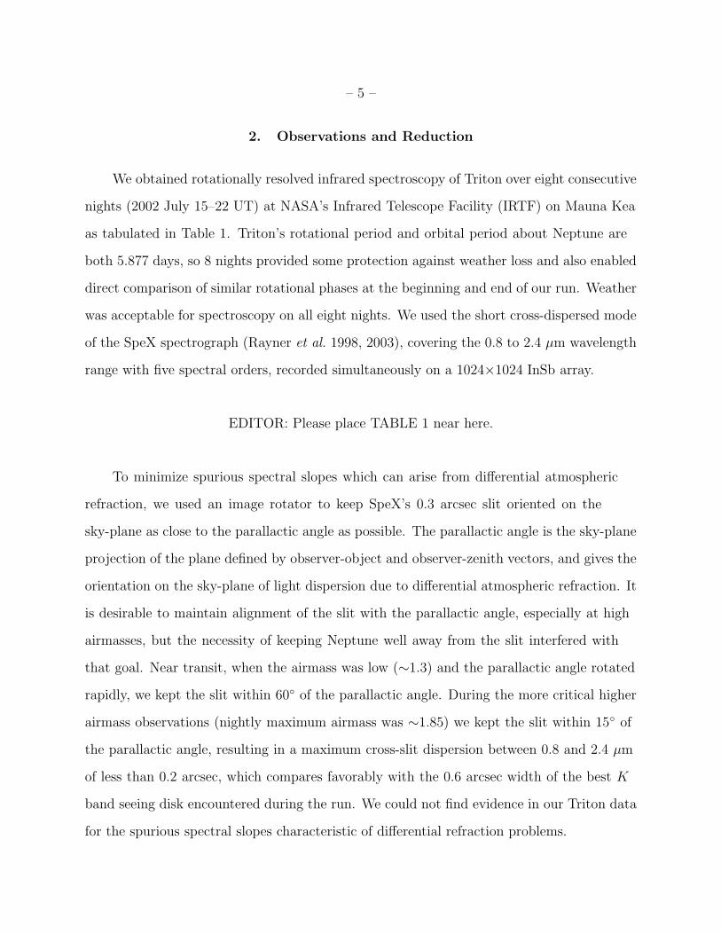
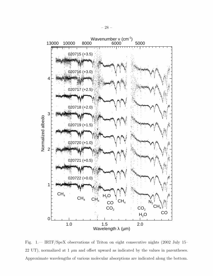
The eight Triton spectra in Fig. 1 appear qualitatively similar to one another, but
close examination reveals subtle differences. The most significant of these is a variation in
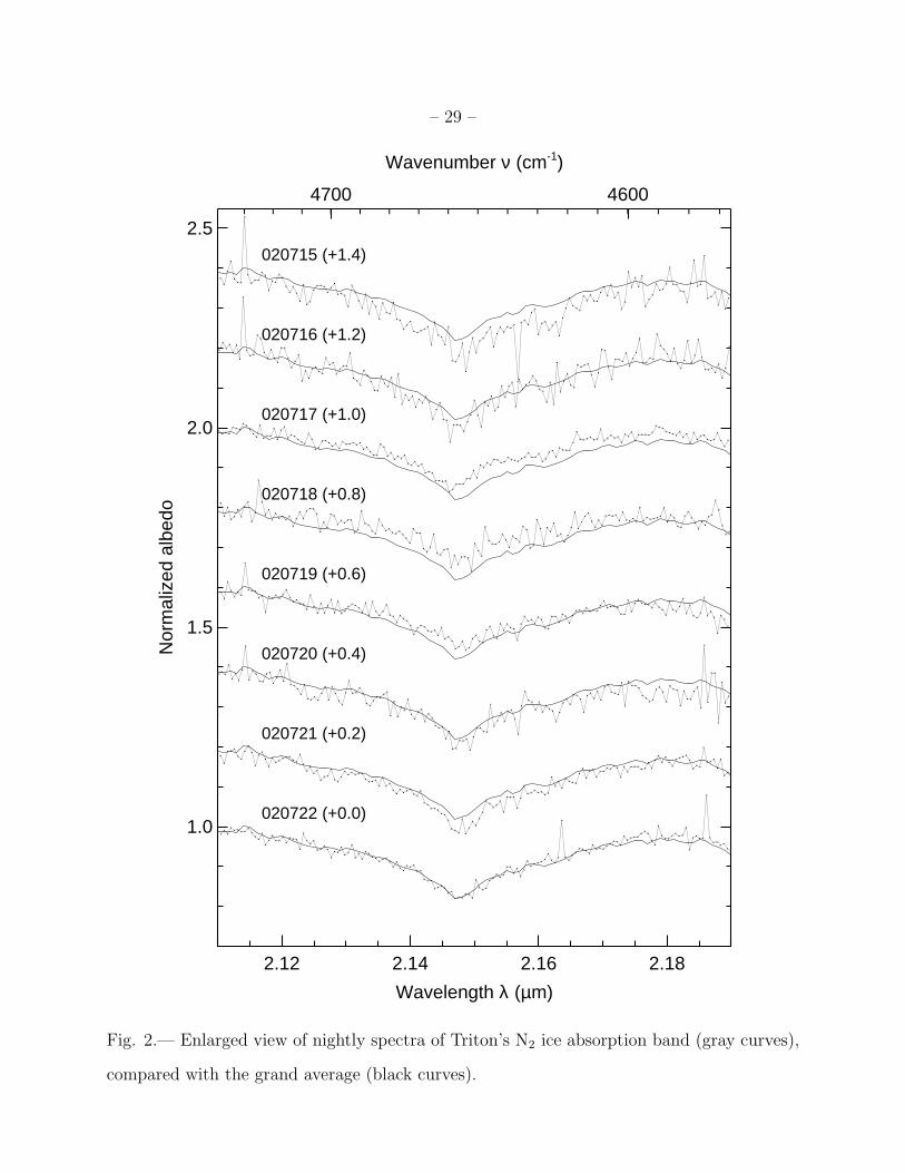
the depth of the β N2 ice absorption band at 2.15 µm, as becomes more apparent in the
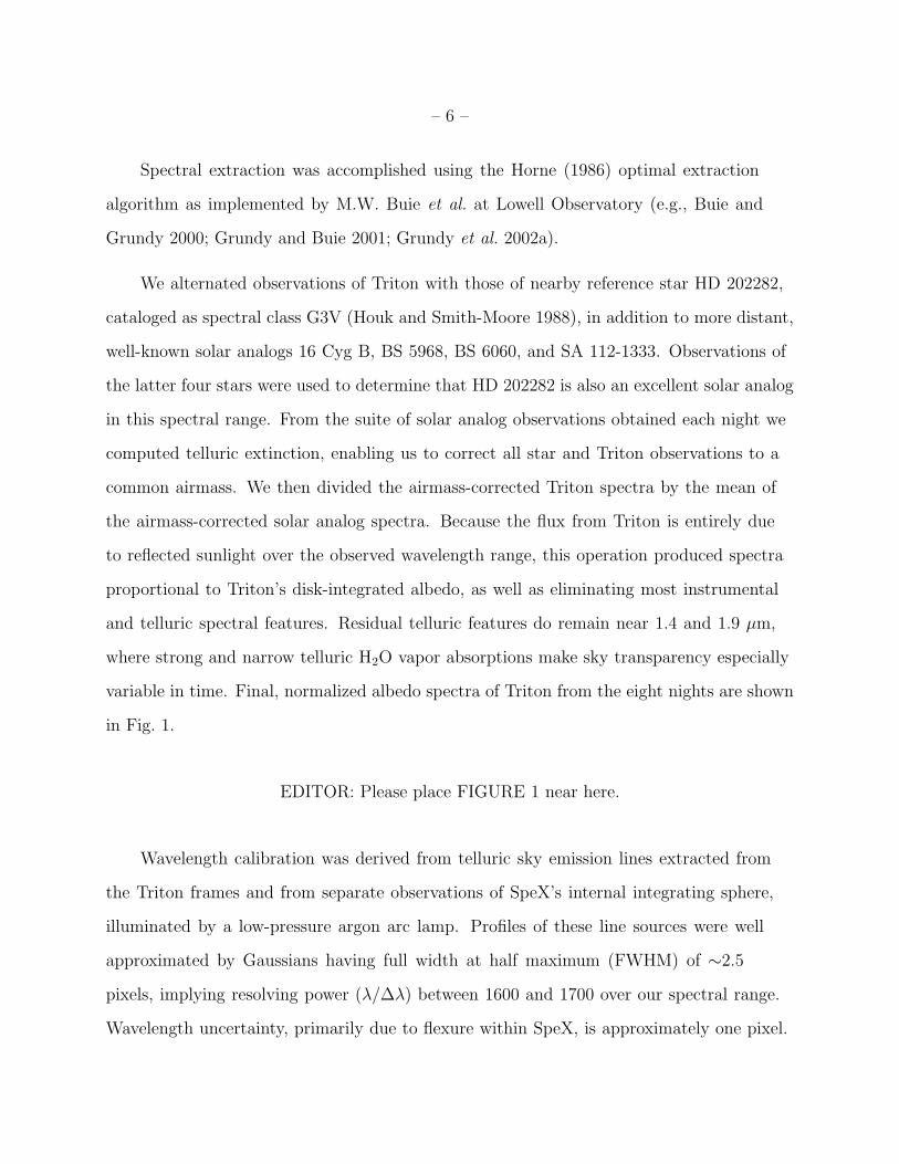
enlarged view in Fig. 2. This variation can be quantified by computing the integrated area
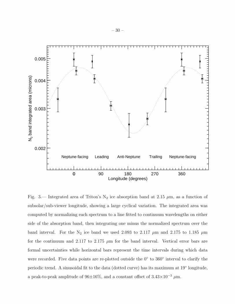
of that band in each night’s spectrum, as plotted versus subsolar longitude in Fig. 3. The
data reveal a nearly-sinusoidal rotational variation with maximum nitrogen absorption seen
when Triton’s Neptune-facing hemisphere is oriented toward the observer. The sinusoidal
best-fit peak-to-peak variation is 96±16%.
EDITOR: Please place FIGURE 2 near here.
EDITOR: Please place FIGURE 3 near here.
– 8 –
This nearly factor of two rotational variation in Triton’s N2 absorption band could
result from numerous possible physical variations with longitude on Triton. For instance,
as seen from Earth, a factor of two change in Triton’s N2 ice-covered projected area as
Triton spins on its axis could cause a factor of two change in the observed absorption band.
A longitudinal change in thickness of a nitrogen ice glaze could have a similar effect, as
could a change in the density of scattering centers or absorbing particles embedded in such
a glaze (e.g., Eluszkiewicz 1991; Duxbury et al. 1997; Eluszkiewicz and Moncet 2003). If
Triton’s nitrogen ice is granular, a change in its mean grain size with longitude could also
produce the observed variation.
Triton’s subsolar (and sub-Earth) latitude during the time of our observations was
−50◦, near the peak of a maximum southern summer (e.g., Trafton 1984; Forget et al.
2000). Regardless of the specific origin of the variation in N2 mean optical path length
as Triton rotates, such high sub-observer latitudes tend to suppress rotational variations
because much of the observable hemisphere remains in continuous view. Only regions north
of −40◦ latitude actually rotate out of view as Triton spins, but being foreshortened by
proximity to Triton’s limb, these regions can only contribute modestly to the total surface
area projected towards Earth. Higher southern latitude regions remain in continuous view,
with their projected areas varying as Triton rotates, but their ability to produce rotational
variations diminishes sharply with proximity to the pole.
EDITOR: Please place FIGURE 4 near here.
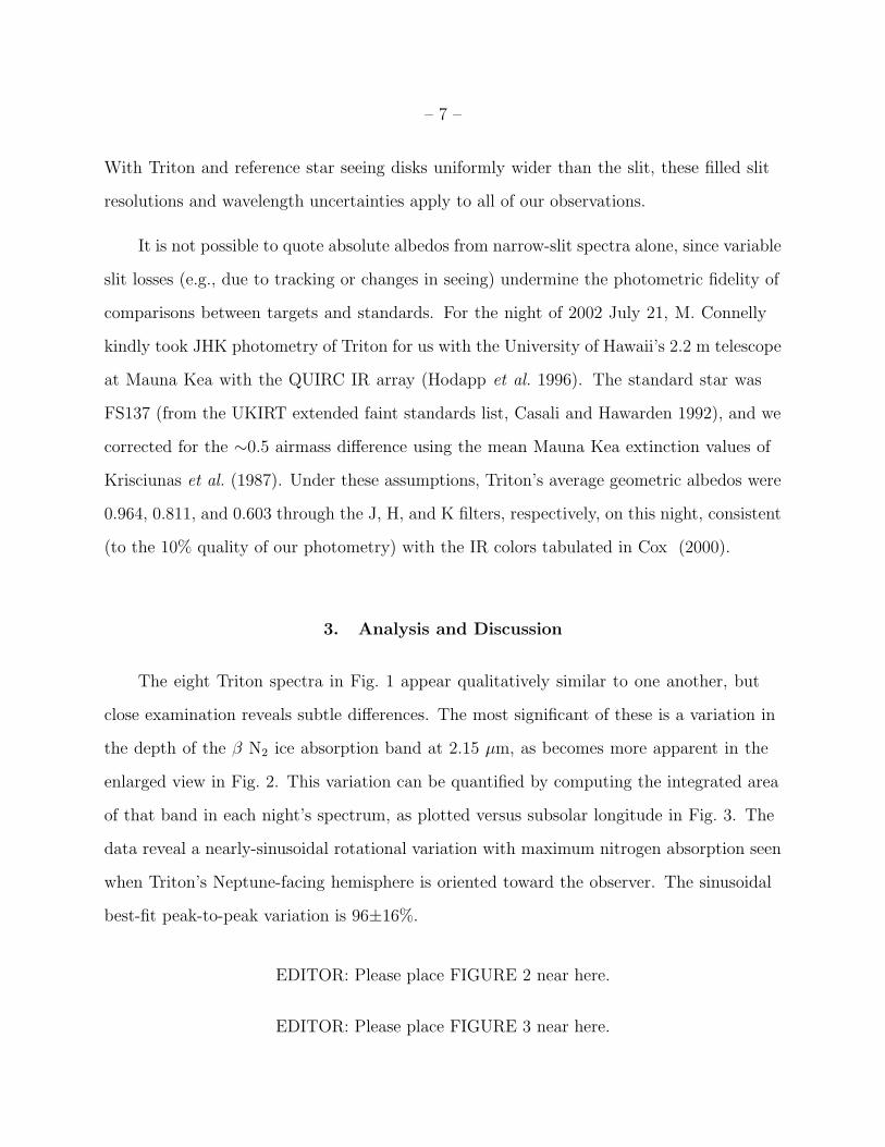
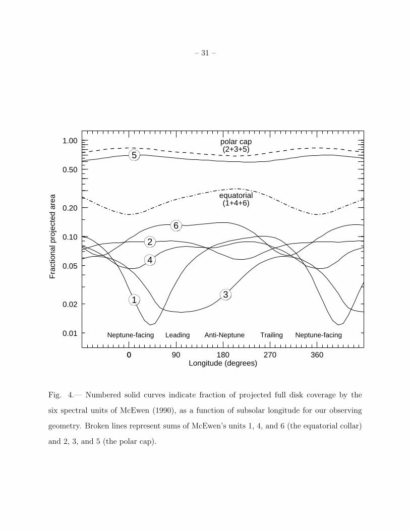
To determine if a previously identified compositional unit on Triton could produce
the observed rotational variation of the N2 band, we plotted in Fig. 4 fractional projected
areas versus subsolar longitude at the epoch of our observations for the six spectral units
mapped by McEwen (1990) from Voyager II clear, green, and violet filter images (see also
– 9 –
Flynn et al. 1996). These units can be divided into two general classes. Triton’s south
polar cap comprises units 2, 3, and 5, while units 1, 4, and 6 are located in an equatorial
band. From volatile transport models, N2 ice is expected to be currently condensing at
equatorial latitudes and sublimating away from high southern latitudes (e.g., Stansberry et
al. 1990; Hansen and Paige 1992). However, all three equatorial band units are best seen
when Triton’s anti-Neptune hemisphere is oriented toward Earth, opposite the observed
behavior of the N2 ice bands. These data strongly imply that McEwen’s three equatorial
collar components are not the regions of Triton responsible for producing the observed
2.15 µm N2 absorption band.
Unit 5 is the only McEwen spectral unit having its minimum and maximum projected
areas coinciding in longitude with the observed N2 band minimum and maximum. This
unit comprises the bulk of Triton’s polar cap. However, the peak-to-peak amplitude of
unit 5’s projected area variation is only about 21%, far below the factor of two variation
exhibited by Triton’s N2 absorption band. If N2 ice were uniformly distributed in unit 5
(optionally including any combination of minority polar cap units 2 and 3), it could not
vary as dramatically with sub-viewer longitude as is observed. If the N2 ice responsible
for Triton’s N2 band is predominantly located on the polar cap, it must not be uniformly
distributed across the cap. A possible resolution is that since the time of the Voyager
encounter in 1989, N2 ice could have sublimated away from high southern latitudes of the
cap. If a large, pole-centered, symmetric patch of the southern cap has lost its N2 ice, the
longitudinal variations arising from the shape of the edge of the cap would be enhanced.
To reach a factor of two variation in projected area, the devolatilized region would need to
extend from the southern pole to about −31◦ latitude.
Significant high latitude N2 ice sublimation loss is to be expected during major summers
on Triton. N2 ice should sublimate away at rates as high as a few cm per Earth year (e.g.

– 10 –
Spencer 1990; Stansberry et al. 1990; Hansen and Paige 1992; Grundy and Stansberry
2000), so several tens of cm of N2 ice could have disappeared from high southern latitudes
between the time of the Voyager encounter (1989 August) and the present observations
(2002 July). Triton’s total surface inventory of N2 ice is not known, but it is possible that
southern polar regions were coated by such a thin layer of N2 ice at the time of the Voyager
encounter. Alternatively, the N2 ice at high southern latitudes could have mechanically
evolved to a state which has a much higher density of scattering centers, resulting in shorter
mean optical path lengths and thus little contribution to the formation of the 2.15 µm N2
ice band, which requires mean optical path lengths of several cm. It is also possible that N2
ice condenses as a thin glaze, invisible at the visual wavelengths explored by Voyager (e.g.,
Duxbury et al. 1997; Eluszkiewicz and Moncet 2003). This condensation need not respect
the boundaries of geological or spectral units. It would simply condense wherever thermal
emission exceeds absorbed solar insolation, tending to favor higher albedo regions and
(currently) more northerly latitudes (e.g., Moore and Spencer 1990; Trafton et al. 1998).
The edge of Triton’s bright polar cap which extends especially close to the equator on the
Neptune-facing hemisphere could be an especially favorable site for N2 condensation. Under
this scenario, high southern latitudes could have been free of N2 ice even at the time of the
Voyager encounter.
EDITOR: Please place FIGURE 5 near here.
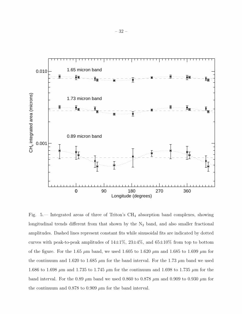
Additional clues can be gleaned from examination of Triton’s other near-infrared
spectral features as functions of subsolar longitude. More subtle rotational variations can
be seen in Triton’s CH4 ice absorption bands, three of which are shown in Fig. 5. The
longitudinal variation of the 0.89, 1.65, and 1.73 µm CH4 bands have best fit sinusoidal
peak-to-peak amplitudes of 65±10%, 14±1% and 23±4%, respectively. Since there is strong
spectroscopic evidence that Triton’s CH4 is highly diluted in N2 ice (e.g., Cruikshank
– 11 –
et al. 1993; Quirico et al. 1999, and also this work), it is perhaps somewhat surprising
not to see more similar rotational variation patterns for Triton’s CH4 and N2 absorption
bands. This evidence for different longitudinal distributions, possibly caused by different
concentrations of CH4 in Triton’s N2 ice, demands explanation. More subtle differences in
longitudinal variability of different CH4 bands offer equally important clues, with weaker
CH4 bands (such as the one at 0.89 µm) apparently showing more pronounced variability
than the stronger bands. The weaker bands require greater optical path lengths to produce
observable absorption, so they are more sensitive to higher CH4 concentrations. For Pluto,
differences in longitudinal variability have also been reported between N2 and CH4, and
between different CH4 bands, and have been interpreted as evidence for compositionally
distinct reservoirs of CH4-bearing ice (Grundy and Buie 2001). Concentration of CH4
in N2 ice is likely to be related to local sublimation and condensation history, with CH4
gradually becoming more concentrated in ice undergoing sublimation, by means of solid
state distillation (e.g., Trafton et al. 1998; Grundy and Stansberry 2000).
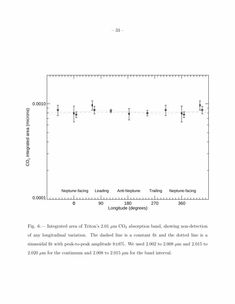
EDITOR: Please place FIGURE 6 near here.
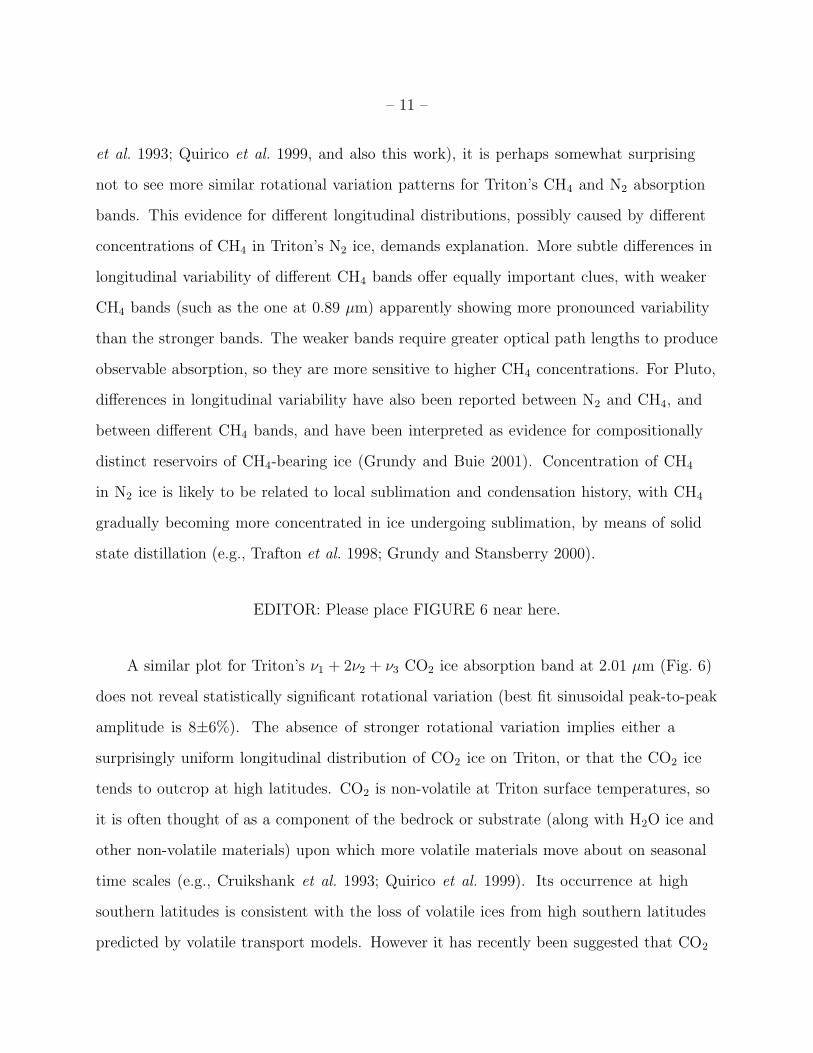
A similar plot for Triton’s ν1 + 2ν2 + ν3 CO2 ice absorption band at 2.01 µm (Fig. 6)
does not reveal statistically significant rotational variation (best fit sinusoidal peak-to-peak
amplitude is 8±6%). The absence of stronger rotational variation implies either a
surprisingly uniform longitudinal distribution of CO2 ice on Triton, or that the CO2 ice
tends to outcrop at high latitudes. CO2 is non-volatile at Triton surface temperatures, so
it is often thought of as a component of the bedrock or substrate (along with H2O ice and
other non-volatile materials) upon which more volatile materials move about on seasonal
time scales (e.g., Cruikshank et al. 1993; Quirico et al. 1999). Its occurrence at high
southern latitudes is consistent with the loss of volatile ices from high southern latitudes
predicted by volatile transport models. However it has recently been suggested that CO2
– 12 –
may move about on seasonal time scales as well, not by sublimation and condensation, but
via aeolian transport (Grundy et al. 2002a). The small amplitude of observed longitudinal
variation in Triton’s CO2 bands would also be consistent with widely distributed CO2 dust.
Similar techniques could not be used to quantify the longitudinal dependence of Triton’s
CO ice because it has only two absorption bands in our spectra, both at inconvenient
wavelengths. The 0-2 transition at 2.35 µm is flanked by strong CH4 bands so the continuum
level could not be determined accurately. The 0-3 transition at 1.58 µm is entangled with a
CO2 ice absorption band and the edge of a H2O ice band complex.
EDITOR: Please place FIGURE 7 near here.
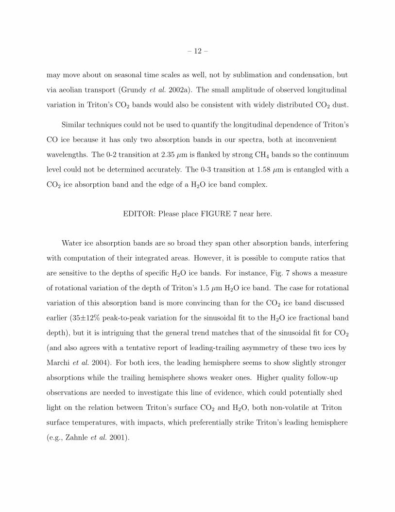
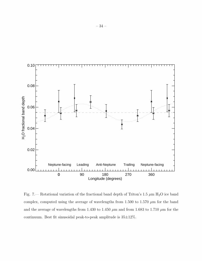
Water ice absorption bands are so broad they span other absorption bands, interfering
with computation of their integrated areas. However, it is possible to compute ratios that
are sensitive to the depths of specific H2O ice bands. For instance, Fig. 7 shows a measure
of rotational variation of the depth of Triton’s 1.5 µm H2O ice band. The case for rotational
variation of this absorption band is more convincing than for the CO2 ice band discussed
earlier (35±12% peak-to-peak variation for the sinusoidal fit to the H2O ice fractional band
depth), but it is intriguing that the general trend matches that of the sinusoidal fit for CO2
(and also agrees with a tentative report of leading-trailing asymmetry of these two ices by
Marchi et al. 2004). For both ices, the leading hemisphere seems to show slightly stronger
absorptions while the trailing hemisphere shows weaker ones. Higher quality follow-up
observations are needed to investigate this line of evidence, which could potentially shed
light on the relation between Triton’s surface CO2 and H2O, both non-volatile at Triton
surface temperatures, with impacts, which preferentially strike Triton’s leading hemisphere
(e.g., Zahnle et al. 2001).
– 13 –
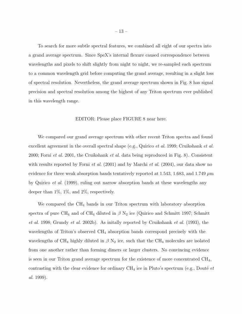
To search for more subtle spectral features, we combined all eight of our spectra into
a grand average spectrum. Since SpeX’s internal flexure caused correspondence between
wavelengths and pixels to shift slightly from night to night, we re-sampled each spectrum
to a common wavelength grid before computing the grand average, resulting in a slight loss
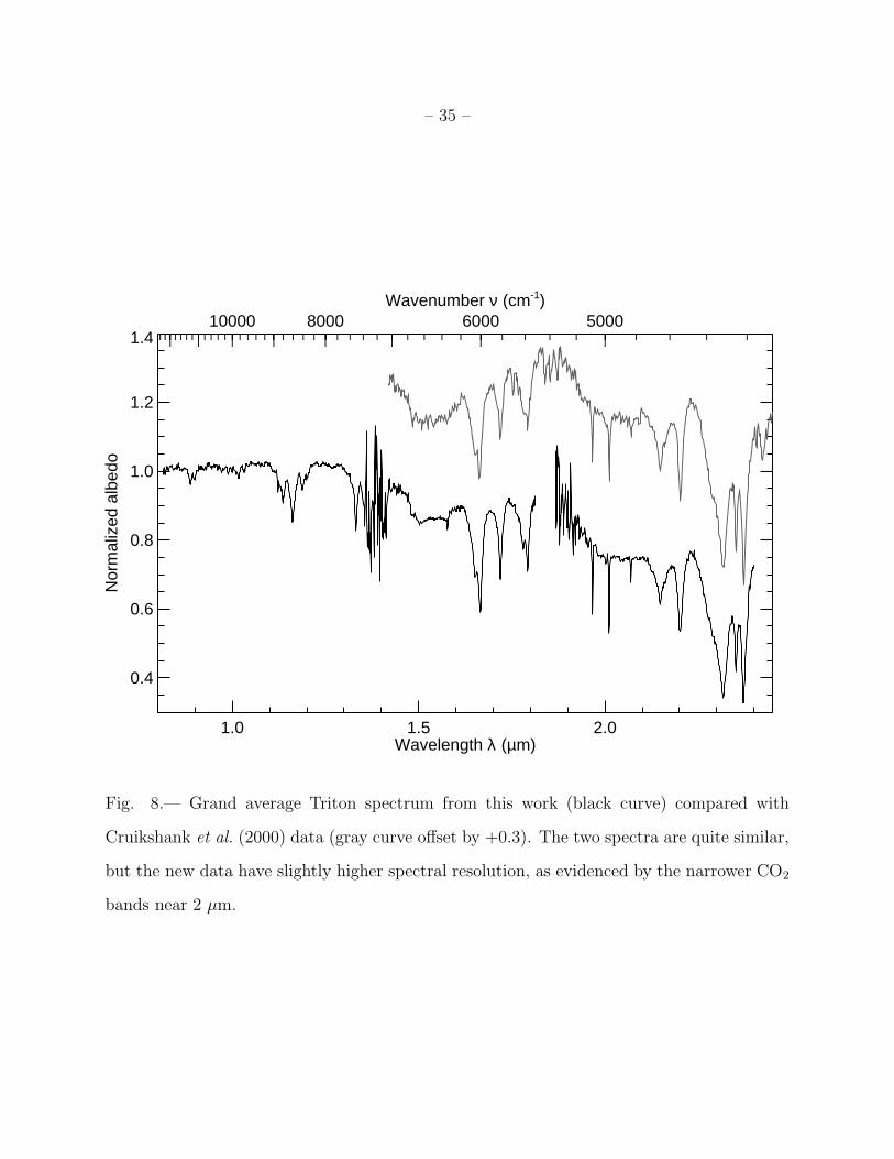
of spectral resolution. Nevertheless, the grand average spectrum shown in Fig. 8 has signal
precision and spectral resolution among the highest of any Triton spectrum ever published
in this wavelength range.
EDITOR: Please place FIGURE 8 near here.
We compared our grand average spectrum with other recent Triton spectra and found
excellent agreement in the overall spectral shape (e.g., Quirico et al. 1999; Cruikshank et al.
2000; Forni et al. 2001, the Cruikshank et al. data being reproduced in Fig. 8). Consistent
with results reported by Forni et al. (2001) and by Marchi et al. (2004), our data show no
evidence for three weak absorption bands tentatively reported at 1.543, 1.683, and 1.749 µm
by Quirico et al. (1999), ruling out narrow absorption bands at these wavelengths any
deeper than 1%, 1%, and 2%, respectively.
We compared the CH4 bands in our Triton spectrum with laboratory absorption
spectra of pure CH4 and of CH4 diluted in β N2 ice (Quirico and Schmitt 1997; Schmitt
et al. 1998; Grundy et al. 2002b). As initally reported by Cruikshank et al. (1993), the
wavelengths of Triton’s observed CH4 absorption bands correspond precisely with the
wavelengths of CH4 highly diluted in β N2 ice, such that the CH4 molecules are isolated
from one another rather than forming dimers or larger clusters. No convincing evidence
is seen in our Triton grand average spectrum for the existence of more concentrated CH4,
contrasting with the clear evidence for ordinary CH4 ice in Pluto’s spectrum (e.g., Doute et
al. 1999).
– 14 –
EDITOR: Please place FIGURE 9 near here.
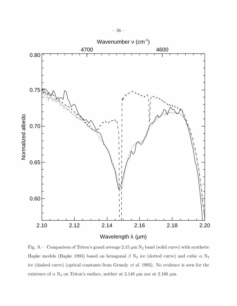
Closer examination of Triton’s nitrogen absorption at 2.15 µm (Fig. 9) shows its shape
to be consistent with the warmer, hexagonal β ice phase, as reported by Cruikshank et al.
(1993). No evidence is seen for the presence of the colder, cubic α N2 phase. However, it
is not possible to rule out the existence of fine-grained α N2; small particles lead to short
mean optical path lengths, and can thus produce negligible spectral contrasts for weak
absorption bands such as these.
EDITOR: Please place FIGURE 10 near here.
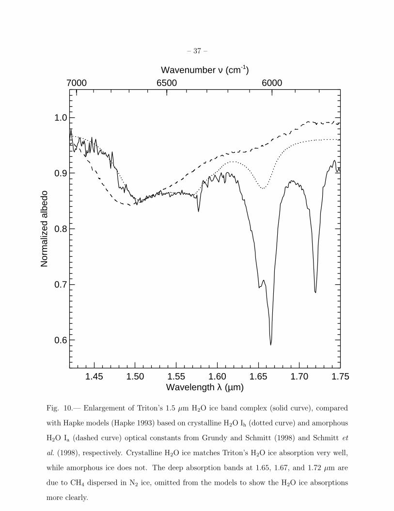
The existence of the temperature-sensitive absorption band at 1.65 µm is the usual
way to distinguish cold crystalline H2O ice from amorphous H2O ice (e.g., Schmitt et al.
1998). A strong CH4 absorption obscures this wavelength in Triton’s spectrum, but the
shape and wavelength of the broader 1.5 µm H2O band can also be used to distinguish the
phase of H2O ice. Comparing our grand average with spectral behavior of crystalline and
amorphous H2O ice in Fig. 10, it is clear from the band’s wavelength and convex-shaped
bottom that Triton’s water ice is predominantly crystalline. This result was tentatively
reported by Cruikshank et al. (2000), and our new data now make this conclusion quite
firm. That H2O ice on Triton’s surface should be crystalline might not have been expected,
since the surface temperature is low enough for H2O ice to remain amorphous over the
age of the solar system (Jenniskens et al. 1998). Its crystallinity is probably indicative of
warmer formation conditions for Triton’s H2O ice.
– 15 –
4. Conclusion
New 0.8-2.4 µm spectral observations of Neptune’s major satellite Triton obtained at
IRTF/SpeX on eight consecutive nights in 2002 reveal periodic variations in the strengths of
absorptions bands of Triton’s surface ices: N2, CH4, and H2O, but not CO2. The observed
variations (or lack thereof) give an indication of how these four ice species are distributed
in longitude. The most heterogeneously distributed ice is N2, which shows twice as much
absorption on Triton’s Neptune-facing hemisphere as on the anti-Neptune hemisphere.
Comparison with maps of Triton’s spectral units made from Voyager data suggest that
Triton’s observed N2 ice is concentrated on low-latitude regions of Triton’s polar cap,
which are predominantly located on the Neptune-facing hemisphere. Non-volatile H2O
ice seems to be slightly concentrated on Triton’s leading hemisphere while Triton’s CH4
ice seems to be slightly concentrated on the trailing hemisphere. Triton’s CO2 ice shows
the least longitudinal variation, suggesting that it is either very uniformly distributed or
that it is confined to high latitudes. Additionally, the shape of Triton’s 1.5 µm water ice
band complex clearly shows that Triton’s H2O ice is crystalline, rather than amorphous
in phase, and the shape of Triton’s 2.15 µm N2 ice absorption is entirely consistent with
the warmer, hexagonal β N2 crystalline phase. The wavelengths of Triton’s CH4 ice
absorptions are consistent with Triton’s CH4 being highly diluted in N2 ice, albeit with
longitudinally-variable concentrations. Using this data set as a baseline, we hope to detect
future evolution of Triton’s near-infrared spectrum, on time scales ranging from months to
years.
– 16 –
Acknowledgments: We thank W. Golisch, D. Griep, P. Sears, S.J. Bus, J.T. Rayner, and
K. Crane for assistance with the telescope and with SpeX, M.W. Buie and R.S. Bussmann
for contributing to the reduction pipeline, M. Showalter for the Rings Node’s on-line
ephemeris services, and NASA for its support of the IRTF. Thanks also to M. Connelly for
contributing infrared photometric data from the University of Hawaii 2.2 m telescope, and
to J.K. Hillier and an anonymous reviewer for their constructive reviews. This work was
made possible by National Science Foundation grant AST-0085614 and NASA Planetary
Astronomy grant NAG5-12516 to Southwest Research Institute, and by NASA Planetary
Geology and Geophysics grant NAG5-10159 to Lowell Observatory. We are also grateful to
the free and open source software communities for empowering us with the tools used to
complete this project, notably Linux, the GNU toolkit, TEX, FVWM, Tcl/Tk, TkRat, and
MySQL.
– 17 –
REFERENCES
Brown, G.N. Jr., and W.T. Ziegler 1980. Vapor pressure and heats of vaporization and
sublimation of liquids and solids of interest in cryogenics below 1–atm pressure. Adv.
Cryogenic Eng. 25, 662-670.
Brown, R.H., D.P. Cruikshank, J. Veverka, P. Helfenstein, and J. Eluszkiewicz 1995. Surface
composition and photometric properties of Triton. In Neptune and Triton, Ed. D.P.
Cruikshank, University of Arizona Press, Tucson, 991-1030.
Buie, M.W., and W.M. Grundy 2000. The distribution and physical state of H2O on
Charon. Icarus 148, 324-339.
Buratti, B.J., J.D. Goguen, J. Gibson, and J. Mosher 1994. Historical photometric evidence
for volatile migration on Triton. Icarus 110, 303-314.
Buratti, B.J., M.D. Hicks, and R.L. Newburn Jr. 1999. Does global warming make Triton
blush? Nature 397, 219.
Casali, M.M., and T.G. Hawarden 1992. The JCMT-UKIRT Newsletter 4, 33-35.
Clark, R.N., F.P. Fanale, and A.P. Zent 1983. Frost grain size metamorphism: Implications
for remote sensing of planetary surfaces. Icarus 56, 233-245.
Cox, A.N. 2000. Allen’s astrophysical quantities (4th ed.). AIP Press; Springer, New York.
Cruikshank, D.P., and J. Apt 1984. Methane on Triton: Physical state and distribution.
Icarus 58, 306-311.
Cruikshank, D.P., R.H. Brown, A.T. Tokunaga, R.G. Smith, and J.R. Piscitelli 1988.
Volatiles on Triton: The infrared spectral evidence, 2.0-2.5 microns. Icarus 74,
413-423.
– 18 –
Cruikshank, D.P., T.L. Roush, T.C. Owen, T.R. Geballe, C. de Bergh, B. Schmitt, R.H.
Brown, and M.J. Bartholomew 1993. Ices on the surface of Triton. Science 261,
742-745.
Cruikshank, D.P., B. Schmitt, T.L. Roush, T.C. Owen, E. Quirico, T.R. Geballe, C.
de Bergh, M.J. Bartholomew, C.M. Dalle Ore, S. Doute, and R. Meier 2000. Water
ice on Triton. Icarus 147, 309-316.
Delitsky, M.L., and W.R. Thompson 1987. Chemical processes in Triton’s atmosphere and
surface. Icarus 70, 354-365.
Doute, S., B. Schmitt, E. Quirico, T.C. Owen, D.P. Cruikshank, C. de Bergh, T.R. Geballe,
and T.L. Roush 1999. Evidence for methane segregation at the surface of Pluto.
Icarus 142, 421-444.
Duxbury, N.S., R.H. Brown, and V. Anicich 1997. Condensation of nitrogen: Implications
for Pluto and Triton. Icarus 129, 202-206.
Elliot, J.L., H.B. Hammel, L.H. Wasserman, O.G. Franz, S.W. McDonald, M.J. Person, C.B.
Olkin, E.W. Dunham, J.R. Spencer, J.A. Stansberry, M.W. Buie, J.M. Pasachoff,
B.A. Babcock, and T.H. McConnochie 1998. Global warming on Triton. Nature 393,
765-767.
Elliot, J.L., M.J. Person, S.W. McDonald, M.W. Buie, E.W. Dunham, R.L. Millis, R.A. Nye,
C.B. Olkin, L.H. Wasserman, L.A. Young, W.B. Hubbard, R. Hill, H.J. Reitsema,
J.M. Pasachoff, T.H. McConnochie, B.A. Babcock, R.C. Stone, and P. Francis 2000a.
The prediction and observation of the 1997 July 18 stellar occultation by Triton:
More evidence for distortion and increasing pressure in Triton’s atmosphere. Icarus
148, 347-369.

– 19 –
Elliot, J.L., D.F. Strobel, X. Zhu, J.A. Stansberry, L.H. Wasserman, and O.G. Franz 2000b.
The thermal structure of Triton’s middle atmosphere. Icarus 143, 425-428.
Eluszkiewicz, J. 1991. On the microphysical state of the surface of Triton. J. Geophys. Res.
96, 19219-19229.
Eluszkiewicz, J., J. Leliwa-Kopystynski, and K.J. Kossacki 1998. Metamorphism of Solar
System Ices. In Solar System Ices, Ed. B. Schmitt, C. de Bergh, and M. Festou,
Kluwer Academic Publishers, Boston, 119-138.
Eluszkiewicz, E., and J.L. Moncet 2003. A coupled microphysical/radiative transfer model
of albedo and emissivity of planetary surfaces covered by volatile ices. Icarus 166,
375-384.
Flynn, B., A. Stern, B. Buratti, P. Schenk, L. Trafton, and J. Mosher 1996. The spatial
distribution of UV-absorbing regions on Triton. Planet. Space Sci. 44, 1039-1046.
Forni, O., S. Le Mouelic, E. Quirico, C. de Bergh, F. Marchis, B. Schmitt, S. Doute, R.
Prange, and L. d’Hendecourt 2001. Near-infrared spectral observations of Triton.
Lunar and Planetary Sci. XXXII, 1275 (abstract).
Forget, F., N. Decamp, C. Le Guyader 2000. A new model for the seasonal evolution of
Triton. Bull. Am. Astron. Soc. 32, 1082 (abstract).
Grundy, W.M., B. Schmitt, and E. Quirico 1993. The temperature dependent spectra of α
and β nitrogen ice with application to Triton. Icarus 105, 254-258.
Grundy, W.M., M.W. Buie, and J.R. Spencer 2002a. Spectroscopy of Pluto and Triton at
3-4 microns: Possible evidence for wide distribution of non-volatile solids. Astron. J.
124, 2273-2278.
– 20 –
Grundy W.M., B. Schmitt, and E. Quirico 2002b. The temperature dependent spectrum of
methane ice I between 0.65 and 5 microns and opportunities for near-infrared remote
thermometry. Icarus 155, 486-496.
Grundy, W.M., and M.W. Buie 2001. Distribution and evolution of CH4, N2, and CO ices
on Pluto’s surface: 1995 to 1998. Icarus 153, 248-263.
Grundy, W.M., and B. Schmitt 1998. The temperature-dependent near-infrared absorption
spectrum of hexagonal H2O ice. J. Geophys. Res. 103, 25809-25822.
Grundy, W.M., and J.A. Stansberry 2000. Solar gardening and the seasonal evolution of
nitrogen ice on Triton and Pluto. Icarus 148, 340-346.
Hansen, C.J., and D.A. Paige 1992. A thermal model for the seasonal nitrogen cycle on
Triton. Icarus 99, 273-288.
Hapke, B. 1993. Theory of reflectance and emittance spectroscopy. Cambridge University
Press, New York.
Hicks, M.D., and B.J. Buratti 2004. The spectral variability of Triton from 1997-2000.
Icarus, in press.
Hillier, J., J. Veverka, and P. Helfenstein 1991. The wavelength dependence of Triton’s light
curve. J. Geophys. Res. 96, 19211-19215.
Hodapp, K.W., J.L. Hora, D.N.B. Hall, L.L. Cowie, M. Metzger, E. Irwin, K. Vural,
L.J. Kozlowski, S.A. Cabelli, C.Y. Chen, D.E. Cooper, G.L. Bostrup, R.B. Bailey,
and W.E. Kleinhans 1996. The HAWAII Infrared Detector Arrays: Testing and
Astronomical Characterization of Prototype and Science Grade Devices. New
Astronomy 1, 177-196.
– 21 –
Horne, K. 1986. An optimal extraction algorithm for CCD spectroscopy. Pub. Astron. Soc.
Pacific 98, 609-617.
Houk, N., and M. Smith-Moore 1988. Catalogue of two-dimensional spectral types for the
HD stars. Vol. 4. Dept. of Astronomy, Univ. of Michigan, Ann Arbor MI.
Hudson, R.L., and M.H. Moore 2001. Radiation chemical alterations in solar system ices:
An overview. J. Geophys. Res. 106, 33275-33284.
Jenniskens, P., DF. Blake, and A. Kouchi 1998. Amorphous water ice: A solar system
material. In Solar System Ices, Ed. B. Schmitt, C. de Bergh, and M. Festou, Kluwer
Academic Publishers, Boston, 139-155.
Johnson, R.E. 1989. Effect of irradiation on the surface of Pluto. Geophys. Res. Lett. 16,
1233-1236.
Krisciunas, K., W. Sinton, D. Tholen, A. Tokunaga, W. Golisch, D. Griep, C. Kaminski, C.
Impey, and C. Christian 1987. Atmospheric Extinction and Night-Sky Brightness at
Mauna Kea. Publ. Astron. Soc. Pacific 99, 887-894.
Marchi, S., C. Barbieri, M. Lazzarin, T.C. Owen, and E.M. Corsini 2004. A 0.4–2.5 µm
spectroscopic investigation of Triton’s two faces. Icarus 168, 367-373.
McDonald, G.D., W.R. Thompson, M. Heinrich, B.N. Khare, and C. Sagan 1994. Chemical
investigation of Titan and Triton tholins. Icarus 108, 137-145.
McEwen, A.S. 1990. Global color and albedo variations on Triton. Geophys. Res. Lett. 17,
1765-1768.
Moore, J.M., and J.R. Spencer 1990. Koyaanismuuyaw: The hypothesis of a perennially
dichotomous Triton. Geophys. Res. Lett. 17, 1757-1760.
– 22 –
Moore, M.H., and R.L. Hudson 2003. Infrared study of ion-irradiated N2-dominated ices
relevant to Triton and Pluto: Formation of HCN and HNC. Icarus 161, 486-500.
Quirico, E., and B. Schmitt 1997. Near-infrared spectroscopy of simple hydrocarbons and
carbon oxides diluted in solid N2 and as pure ices: Implications for Triton and Pluto.
Icarus 127, 354-378.
Quirico, E., S. Doute, B. Schmitt, C. de Bergh, D.P. Cruikshank, T.C. Owen, T.R. Geballe,
and T.L. Roush 1999. Composition, physical state, and distribution of ices at the
surface of Triton. Icarus 139, 159-178.
Rayner, J.T., D.W. Toomey, P.M. Onaka, A.J. Denault, W.E. Stahlberger, D.Y. Watanabe,
and S.I. Wang 1998. SpeX: A medium-resolution IR spectrograph for IRTF. Proc.
SPIE 3354, 468-479.
Rayner, J.T., D.W. Toomey, P.M. Onaka, A.J. Denault, W.E. Stahlberger, W.D. Vacca,
M.C. Cushing, and S. Wang 2003. SpeX: A medium-resolution 0.8–5.5 micron
spectrograph and imager for the NASA Infrared Telescope Facility. Publ. Astron.
Soc. Pacific 115, 362-382.
Salama, F., 1998. UV photochemistry of ices. In Solar System Ices, Ed. B. Schmitt, C.
de Bergh, and M. Festou, Kluwer Academic Publishers, Boston, 259-279.
Schmitt, B., E. Quirico, F. Trotta, and W.M. Grundy 1998. Optical properties of ices from
UV to infrared. In Solar System Ices, Ed. B. Schmitt, C. de Bergh, and M. Festou,
Kluwer Academic Publishers, Boston, 199-240.
Spencer, J.R. 1990. Nitrogen frost migration on Triton: A historical model. Geophys. Res.
Lett. 17, 1769-1772.
– 23 –
Spencer, J.R., and J.M. Moore 1992. The influence of thermal inertia on temperatures and
frost stability on Triton. Icarus 99, 261-272.
Stansberry, J.A., J.I. Lunine, C.C. Porco, and A.S. McEwen 1990. Zonally averaged thermal
balance and stability models for nitrogen polar caps on Triton. Geophys. Res. Lett.
17, 1773-1776.
Strazzulla, G., 1998. Chemistry of ice induced by bombardment with energetic charged
particles. In Solar System Ices, Ed. B. Schmitt, C. de Bergh, and M. Festou, Kluwer
Academic Publishers, Boston, 281-301.
Trafton, L. 1984. Large seasonal variations in Triton’s atmosphere. Icarus 58, 312-324.
Trafton, L.M., D.L. Matson, and J.A. Stansberry 1998. Surface/atmosphere interactions
and volatile transport (Triton, Pluto, and Io). In Solar System Ices, Ed. B. Schmitt,
C. de Bergh, and M. Festou, Kluwer Academic, Boston, 773-812.
Young, L.A., and S.A. Stern 2001. Ultraviolet observations of Triton in 1999 with the
space telescope imaging spectrograph: 2150-3180 A spectroscopy and disk-integrated
photometry. Astron. J. 122, 449-456.
Zahnle, K., P. Schenk, S. Sobieszczyk, L. Dones, and H.F. Levison 2001. Differential
cratering of synchronously rotating satellites by ecliptic comets. Icarus 153, 111-129.
– 24 –
Table 1. Circumstances of observations
UT date of Transparency and Subsolar Phase Total
observation K band seeing longitude angle integration
mid-time conditions (◦) (◦) (min)
2002/07/15.39 Clear, 1.0′′ 359.8 0.58 52
2002/07/16.39 Scattered clouds, 0.8′′ 61.1 0.55 52
2002/07/17.41 Cirrus, 0.7′′ 123.6 0.52 84
2002/07/18.40 Thin high clouds, 1.2′′ 184.1 0.49 64
2002/07/19.40 Some thin cirrus, 0.8′′ 245.2 0.46 68
2002/07/20.39 Some thin cirrus, 0.7′′ 306.3 0.42 68
2002/07/21.40 Some thin cirrus, 0.6′′ 7.6 0.39 68
2002/07/22.39 Very clear, 0.8′′ 68.5 0.36 84
– 25 –
FIGURE CAPTIONS
Fig. 1.— IRTF/SpeX observations of Triton on eight consecutive nights (2002 July 15–
22 UT), normalized at 1 µm and offset upward as indicated by the values in parentheses.
Approximate wavelengths of various molecular absorptions are indicated along the bottom.
Fig. 2.— Enlarged view of nightly spectra of Triton’s N2 ice absorption band (gray curves),
compared with the grand average (black curves).
Fig. 3.— Integrated area of Triton’s N2 ice absorption band at 2.15 µm, as a function of
subsolar/sub-viewer longitude, showing a large cyclical variation. The integrated area was
computed by normalizing each spectrum to a line fitted to continuum wavelengths on either
side of the absorption band, then integrating one minus the normalized spectrum over the
band interval. For the N2 ice band we used 2.093 to 2.117 µm and 2.175 to 1.185 µm
for the continuum and 2.117 to 2.175 µm for the band interval. Vertical error bars are
formal uncertainties while horizontal bars represent the time intervals during which data
were recorded. Five data points are re-plotted outside the 0◦ to 360◦ interval to clarify the
periodic trend. A sinusoidal fit to the data (dotted curve) has its maximum at 19◦ longitude,
a peak-to-peak amplitude of 96±16%, and a constant offset of 3.43×10⁻³ µm.
Fig. 4.— Numbered solid curves indicate fraction of projected full disk coverage by the
six spectral units of McEwen (1990), as a function of subsolar longitude for our observing
geometry. Broken lines represent sums of McEwen’s units 1, 4, and 6 (the equatorial collar)
and 2, 3, and 5 (the polar cap).
Fig. 5.— Integrated areas of three of Triton’s CH4 absorption band complexes, showing
longitudinal trends different from that shown by the N2 band, and also smaller fractional
amplitudes. Dashed lines represent constant fits while sinusoidal fits are indicated by dotted
curves with peak-to-peak amplitudes of 14±1%, 23±4%, and 65±10% from top to bottom
– 26 –
of the figure. For the 1.65 µm band, we used 1.605 to 1.620 µm and 1.685 to 1.699 µm for
the continuum and 1.620 to 1.685 µm for the band interval. For the 1.73 µm band we used
1.686 to 1.698 µm and 1.735 to 1.745 µm for the continuum and 1.698 to 1.735 µm for the
band interval. For the 0.89 µm band we used 0.860 to 0.878 µm and 0.909 to 0.930 µm for
the continuum and 0.878 to 0.909 µm for the band interval.
Fig. 6.— Integrated area of Triton’s 2.01 µm CO2 absorption band, showing non-detection
of any longitudinal variation. The dashed line is a constant fit and the dotted line is a
sinusoidal fit with peak-to-peak amplitude 8±6%. We used 2.002 to 2.008 µm and 2.015 to
2.020 µm for the continuum and 2.008 to 2.015 µm for the band interval.
Fig. 7.— Rotational variation of the fractional band depth of Triton’s 1.5 µm H2O ice band
complex, computed using the average of wavelengths from 1.500 to 1.570 µm for the band
and the average of wavelengths from 1.430 to 1.450 µm and from 1.683 to 1.710 µm for the
continuum. Best fit sinusoidal peak-to-peak amplitude is 35±12%.
Fig. 8.— Grand average Triton spectrum from this work (black curve) compared with
Cruikshank et al. (2000) data (gray curve offset by +0.3). The two spectra are quite similar,
but the new data have slightly higher spectral resolution, as evidenced by the narrower CO2
bands near 2 µm.
Fig. 9.— Comparison of Triton’s grand average 2.15 µm N2 band (solid curve) with synthetic
Hapke models (Hapke 1993) based on hexagonal β N2 ice (dotted curve) and cubic α N2
ice (dashed curve) (optical constants from Grundy et al. 1993). No evidence is seen for the
existence of α N2 on Triton’s surface, neither at 2.148 µm nor at 2.166 µm.
Fig. 10.— Enlargement of Triton’s 1.5 µm H2O ice band complex (solid curve), compared
with Hapke models (Hapke 1993) based on crystalline H2O Ih (dotted curve) and amorphous
H2O Ia (dashed curve) optical constants from Grundy and Schmitt (1998) and Schmitt et
– 27 –
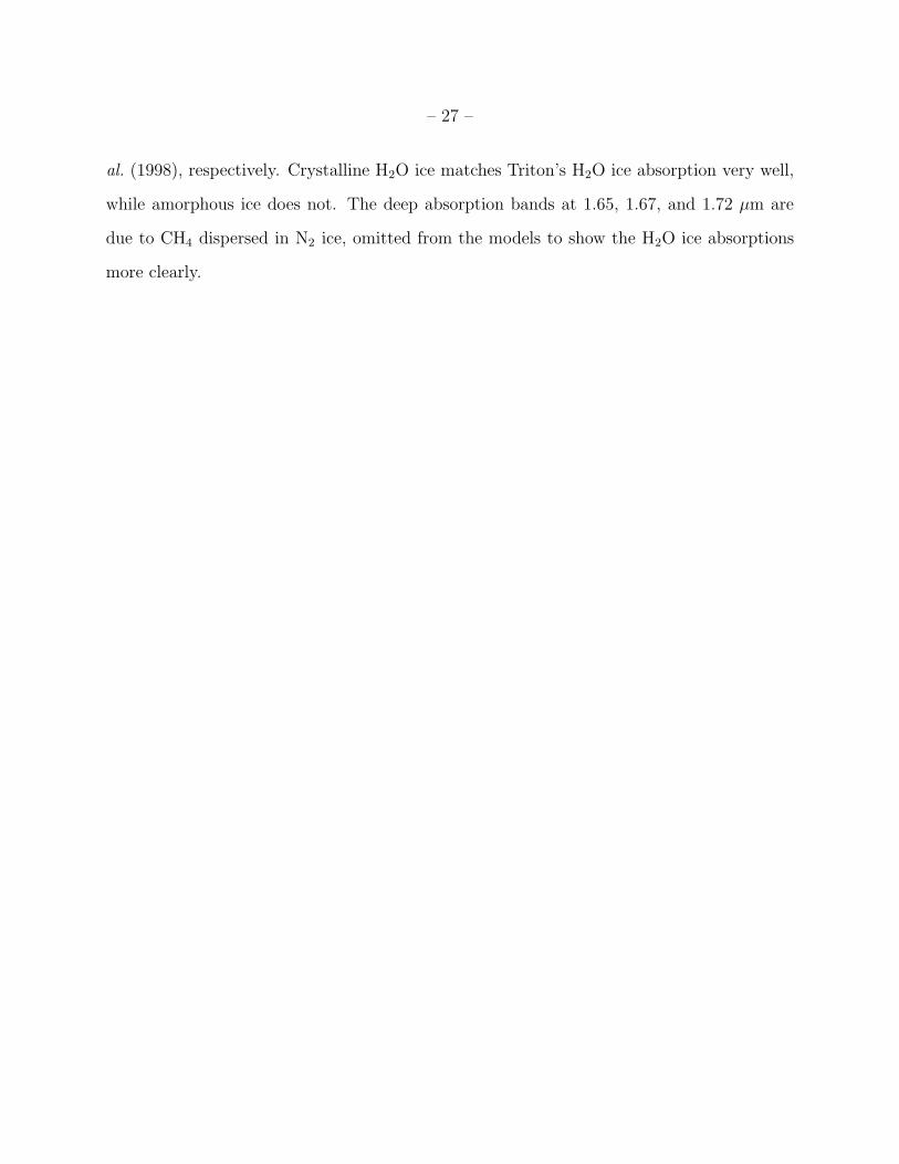
al. (1998), respectively. Crystalline H2O ice matches Triton’s H2O ice absorption very well,
while amorphous ice does not. The deep absorption bands at 1.65, 1.67, and 1.72 µm are
due to CH4 dispersed in N2 ice, omitted from the models to show the H2O ice absorptions
more clearly.
– 28 –
1.0 1.5 2.0
0
1
2
3
4
Nor
mal
ized
alb
edo
Wavelength λ (µm)
Wavenumber ν (cm-1)13000 10000 8000 6000 5000
020722 (+0.0)
020721 (+0.5)
020720 (+1.0)
020719 (+1.5)
020718 (+2.0)
020717 (+2.5)
020716 (+3.0)
020715 (+3.5)
H2O
H2O
CO2 CO2
CH4CH4 CH4 CH4
CH4
N2CO
CO
Fig. 1.— IRTF/SpeX observations of Triton on eight consecutive nights (2002 July 15–
22 UT), normalized at 1 µm and offset upward as indicated by the values in parentheses.
Approximate wavelengths of various molecular absorptions are indicated along the bottom.
– 29 –
2.12 2.14 2.16 2.18
1.0
1.5
2.0
2.5
Nor
mal
ized
alb
edo
Wavelength λ (µm)
Wavenumber ν (cm-1)
4700 4600
020722 (+0.0)
020721 (+0.2)
020720 (+0.4)
020719 (+0.6)
020718 (+0.8)
020717 (+1.0)
020716 (+1.2)
020715 (+1.4)
Fig. 2.— Enlarged view of nightly spectra of Triton’s N2 ice absorption band (gray curves),
compared with the grand average (black curves).
– 30 –
0 90 180 270 360 0Longitude (degrees)
0.002
0.003
0.004
0.005
N2
band
inte
grat
ed a
rea
(mic
rons
)
Neptune-facing Leading Anti-Neptune Trailing Neptune-facing
Fig. 3.— Integrated area of Triton’s N2 ice absorption band at 2.15 µm, as a function of
subsolar/sub-viewer longitude, showing a large cyclical variation. The integrated area was
computed by normalizing each spectrum to a line fitted to continuum wavelengths on either
side of the absorption band, then integrating one minus the normalized spectrum over the
band interval. For the N2 ice band we used 2.093 to 2.117 µm and 2.175 to 1.185 µm
for the continuum and 2.117 to 2.175 µm for the band interval. Vertical error bars are
formal uncertainties while horizontal bars represent the time intervals during which data
were recorded. Five data points are re-plotted outside the 0◦ to 360◦ interval to clarify the
periodic trend. A sinusoidal fit to the data (dotted curve) has its maximum at 19◦ longitude,
a peak-to-peak amplitude of 96±16%, and a constant offset of 3.43×10⁻³ µm.
– 31 –
0 90 180 270 360 0Longitude (degrees)
0.10
0.20
0.50
1.00
0.01
0.02
0.05
Fra
ctio
nal p
roje
cted
are
a
1
2
3
4
5
6
equatorial(1+4+6)
polar cap(2+3+5)
Neptune-facing Leading Anti-Neptune Trailing Neptune-facing
Fig. 4.— Numbered solid curves indicate fraction of projected full disk coverage by the
six spectral units of McEwen (1990), as a function of subsolar longitude for our observing
geometry. Broken lines represent sums of McEwen’s units 1, 4, and 6 (the equatorial collar)
and 2, 3, and 5 (the polar cap).
– 32 –
0 90 180 270 360 0Longitude (degrees)
0.001
0.010
CH
4 in
tegr
ated
are
a (m
icro
ns)
1.65 micron band
1.73 micron band
0.89 micron band
Fig. 5.— Integrated areas of three of Triton’s CH4 absorption band complexes, showing
longitudinal trends different from that shown by the N2 band, and also smaller fractional
amplitudes. Dashed lines represent constant fits while sinusoidal fits are indicated by dotted
curves with peak-to-peak amplitudes of 14±1%, 23±4%, and 65±10% from top to bottom
of the figure. For the 1.65 µm band, we used 1.605 to 1.620 µm and 1.685 to 1.699 µm for
the continuum and 1.620 to 1.685 µm for the band interval. For the 1.73 µm band we used
1.686 to 1.698 µm and 1.735 to 1.745 µm for the continuum and 1.698 to 1.735 µm for the
band interval. For the 0.89 µm band we used 0.860 to 0.878 µm and 0.909 to 0.930 µm for
the continuum and 0.878 to 0.909 µm for the band interval.
– 33 –
0 90 180 270 360 0Longitude (degrees)
0.0001
0.0010
CO
2 in
tegr
ated
are
a (m
icro
ns)
Neptune-facing Leading Anti-Neptune Trailing Neptune-facing
Fig. 6.— Integrated area of Triton’s 2.01 µm CO2 absorption band, showing non-detection
of any longitudinal variation. The dashed line is a constant fit and the dotted line is a
sinusoidal fit with peak-to-peak amplitude 8±6%. We used 2.002 to 2.008 µm and 2.015 to
2.020 µm for the continuum and 2.008 to 2.015 µm for the band interval.
– 34 –
0 90 180 270 360 0Longitude (degrees)
0.00
0.02
0.04
0.06
0.08
0.10
H2O
frac
tiona
l ban
d de
pth
Neptune-facing Leading Anti-Neptune Trailing Neptune-facing
Fig. 7.— Rotational variation of the fractional band depth of Triton’s 1.5 µm H2O ice band
complex, computed using the average of wavelengths from 1.500 to 1.570 µm for the band
and the average of wavelengths from 1.430 to 1.450 µm and from 1.683 to 1.710 µm for the
continuum. Best fit sinusoidal peak-to-peak amplitude is 35±12%.
– 35 –
1.0 1.5 2.0
0.4
0.6
0.8
1.0
1.2
1.4
Nor
mal
ized
alb
edo
Wavelength λ (µm)
Wavenumber ν (cm-1) 10000 8000 6000 5000
Fig. 8.— Grand average Triton spectrum from this work (black curve) compared with
Cruikshank et al. (2000) data (gray curve offset by +0.3). The two spectra are quite similar,
but the new data have slightly higher spectral resolution, as evidenced by the narrower CO2
bands near 2 µm.
– 36 –
2.10 2.12 2.14 2.16 2.18 2.20
0.60
0.65
0.70
0.75
0.80
Nor
mal
ized
alb
edo
Wavelength λ (µm)
Wavenumber ν (cm-1)4700 4600
Fig. 9.— Comparison of Triton’s grand average 2.15 µm N2 band (solid curve) with synthetic
Hapke models (Hapke 1993) based on hexagonal β N2 ice (dotted curve) and cubic α N2
ice (dashed curve) (optical constants from Grundy et al. 1993). No evidence is seen for the
existence of α N2 on Triton’s surface, neither at 2.148 µm nor at 2.166 µm.
– 37 –
1.45 1.50 1.55 1.60 1.65 1.70 1.75
0.6
0.7
0.8
0.9
1.0
Nor
mal
ized
alb
edo
Wavelength λ (µm)
Wavenumber ν (cm-1)7000 6500 6000
Fig. 10.— Enlargement of Triton’s 1.5 µm H2O ice band complex (solid curve), compared
with Hapke models (Hapke 1993) based on crystalline H2O Ih (dotted curve) and amorphous
H2O Ia (dashed curve) optical constants from Grundy and Schmitt (1998) and Schmitt et
al. (1998), respectively. Crystalline H2O ice matches Triton’s H2O ice absorption very well,
while amorphous ice does not. The deep absorption bands at 1.65, 1.67, and 1.72 µm are
due to CH4 dispersed in N2 ice, omitted from the models to show the H2O ice absorptions
more clearly.