NEAREST NEIGHBOR RULE Jeff Robble, Brian Renzenbrink, Doug Roberts

Nearest Neighbor Rule

Consider a test point x. x’ is the closest point to x out of the rest of the test points. Nearest Neighbor Rule selects the class for x with the

assumption that:

Is this reasonable? Yes, if x’ is sufficiently close to x. If x’ and x were overlapping (at the same point), they would

share the same class. As the number of test points increases, the closer x’ will

probably be to x.

Nearest Neighbor Estimation

Possible solution for the unknown “best” window problem   The best window problem involves deciding how to partition the

available data   Let the cell volume be a function of the training data   Instead of an arbitrary function of the overall number of samples

To estimate p(x) from n training samples   Center a cell about a point x   Let the cell grow until kn samples are captured   kn is a specified function of n   Samples are the kn nearest neighbors of the point x

Nearest Neighbor Estimation

  Eq. 1 is the probability of choosing point x given n samples in cell volume Vn   kn goes to infinity as n goes to infinity

  Assures eq. 2 is a good estimate of the probability that a point falls in Vn

  A good estimate of the probability that a point will fall in a cell of volume Vn is eq. 2

  kn must grow slowly in order for the size of the cell needed to capture kn samples to shrink to zero

  Thus eq. 2 must go to zero   These conditions are necessary for pn(x) to converge to p(x) at all points

where p(x) is continuous

(1)

(2)

(3)

(4)

Nearest Neighbor Estimation

The diagram is a 2D representation of Nearest Neighbor applied of a feature space of 1 dimension

The nearest neighbors for k = 3 and k = 5 The slope discontinuities lie away from the prototype points

The diagram is a 3D representation of Nearest Neighbor applied of a feature space of 2 dimensions

The high peaks show the cluster centers The red dots are the data points

Nearest Neighbor Estimation

Nearest Neighbor Estimation

Posterior probabilities can be estimated using a set of n labeled samples to estimate densities

Eq. 5 is used to estimate the posterior probabilities Eq. 5 basically states that ωi is the fraction of samples

within a cell that are labeled ωi

(5)

Choosing the Size of a Cell

Parzen-window approach   Vn is a specified function of n

kn-nearest neighbor   Vn is expanded until a specified number of samples are

captured

Either way an infinite number of samples will fall within an infinitely small cell as n goes to infinity

Voronoi Tesselation

Partition the feature space into cells. Boundary lines lie half-way between any two points. Label each cell based on the class of enclosed point. 2 classes: red, black

Notation

is class with maximum probability given a point

Bayes Decision Rule always selects class which results in minimum risk (i.e. highest probability), which is

P* is the minimum probability of error, which is Bayes Rate.

(37)

(46) Minimum error probability for a given x:

Minimum average error probability for x:

Nearest Neighbor Error

We will show:   The average probability of error is not concerned with

the exact placement of the nearest neighbor.   The exact conditional probability of error is:

  The above error rate is never worse than 2x the Bayes Rate:

Approximate probability of error when all classes, c, have equal probability:

Convergence: Average Probability of Error

Error depends on choosing the a nearest neighbor that shares that same class as x:

As n goes to infinity, we expect p(x’|x) to approach a delta function (i.e. get indefinitely large as x’ nearly overlaps x).

Thus, the integral of p(x’|x) will evaluate to 0 everywhere but at x where it will evaluate to 1, so:

Thus, the average probability of error is not concerned with the nearest neighbor, x’.

(40)

Convergence: Average Probability of Error

At x, assume probability is continuous and not 0. There is a hypersphere, S, (with as many dimensions as

x has features) centered around point x:

Probability that all n test samples drawn fall outside S:

(1-Ps) will produce a fraction. A fraction taken to a large power will decrease. Thus, as n approaches infinity, the above eq. approaches

zero.

Let’s use intuition to explain the delta function.

Probability a point falls inside S:

Error Rate: Conditional Probability of Error

For each of n test samples, there is an error whenever the chosen class for that sample is not the actual class.

For the Nearest Neighbor Rule:   Each test sample is a random (x,θ) pairing, where θ is the actual

class of x.   For each x we choose x’. x’ has class θ’.   There is an error if θ ≠ θ’.

Plugging this into eq. 40 and taking the limit:

delta function: x ≈ x’ (44)

sum over classes being the same for x and x’

Error Rate: Conditional Probability of Error

Error as number of samples go to infinity:

Plugging in eq. 37:

Plugging in eq. 44:

What does eq. 45 mean?

Notice the squared term. The lower the probability of correctly identifying a class given point x,

the greater impact it has on increasing the overall error rate for identifying that point’s class.

It’s an exact result. How does it compare to Bayes Rate, P*?

(45)

Constraint 2:

Error Bounds

Exact Conditional Probability of Error: How low can this get? How high can the error rate get?

Expand:

Constraint 1: eq. 46

Non-m Posterior Probabilities have equal likelihood. Thus, divide by c-1.

The summed term is minimized when all the posterior probabilities but the mth are equal:

Error Bounds

Finding the Error Bounds:

Plug in minimizing conditions and make inequality

Factor

Combine terms

Simplify

Rearrange expression

Error Bounds

Variance: Tightest upper bounds:

(45)

(37)

Finding the Error Bounds:

Integrate both sides with respect to choosing x and plug in the highlighted terms.

Thus, the error rate is less than twice the Bayes Rate.

Found by keeping the right term.

Error Bounds

Bounds on the Nearest Neighbor error rate.

0 ≤ P* ≤ (c-1)/c

When Bayes Rate, P*, is small, the upper bound is approx. 2x Bayes Rate.

With infinite data, and a complex decision rule, you can at most cut the error rate in half.

Difficult to show Nearest Neighbor performance convergence to asymptotic value.

Take P* = 0 and P* = 1 to get bounds for P*

k-Nearest Neighbor Rule

Consider a test point x. is the vector of the k nearest points to x The k-Nearest Neighbor Rule assigns the most frequent

class of the points within . We will study the two-class case. Therefore, k must be an odd number (to prevent ties).

k-Nearest Neighbor Rule

The k-nearest neighbor rule attempts to match probabilities with nature.

As with the single neighbor case, the labels of each of the k-nearest neighbor are random variables.

Bayes decision rule always selects . Recall that the single nearest neighbor case assumes with the probability .

The k-nearest neighbor rule selects with the probability of :

Error Bounds

We can prove that if k is odd, the two-class error rate for the k-nearest neighbor rule has an upper bound of the function where is the smallest concave function of greater than:

Note that the first bracketed term [blue] represents the probability of error due to i points coming from the category having the minimum real probability and k-i>i points from the other category

The second bracketed term [green] represents the probability that k-i points are from the minimum-real probability category and i+1<k-i from the higher probability category.

Error Bounds

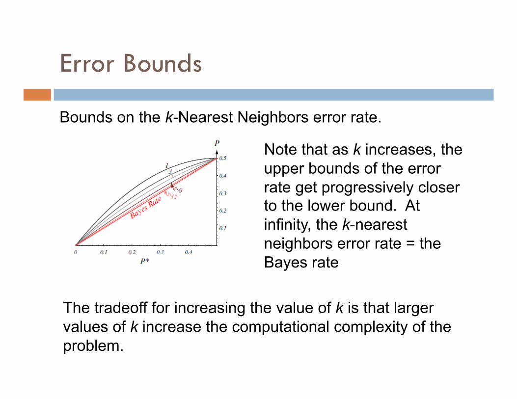
Bounds on the k-Nearest Neighbors error rate.

Note that as k increases, the upper bounds of the error rate get progressively closer to the lower bound. At infinity, the k-nearest neighbors error rate = the Bayes rate

The tradeoff for increasing the value of k is that larger values of k increase the computational complexity of the problem.

Example

Here is a basic example of the k-nearest neighbor algorithm for:

k=3

k=5

Computational Complexity

The computational complexity of the k-nearest neighbor rule has received a great deal of attention. We will focus on cases involving an arbitrary d dimensions. The complexity of the base case where we examine every single node’s distance is O(dn).

There are three general algorithmic techniques for reducing the computational cost of our search:

  Partial Distance calculation   Prestructuring   Editing.

Partial Distance

In the partial distance algorithm, we calculate the distance using some subset r of the full d dimensions. If this partial distance is too great, we stop computing. The partial distance based on r selected dimensions is:

Where r < d.

The partial distance method assumes that the dimensional subspace we define is indicative of the full data space.

The partial distance method is strictly non-decreasing as we add dimensions.

Prestructuring

In prestructuring we create a search tree in which all points are linked. During classification, we compute the distance of the test point to one or a few stored root points and consider only the tree associated with that root. This method requires proper structuring to successfully reduce cost. Note that the method is NOT guaranteed to find the closest prototype.

Editing

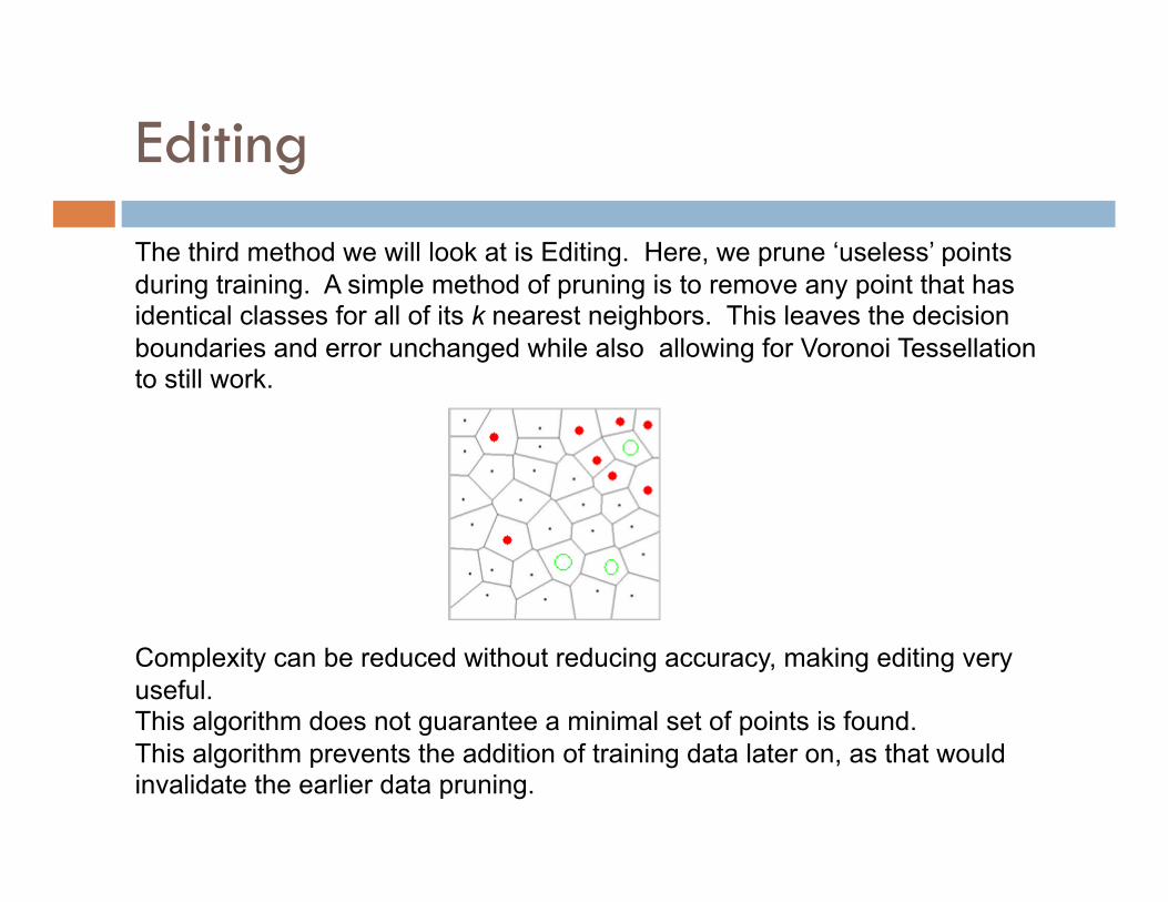
The third method we will look at is Editing. Here, we prune ‘useless’ points during training. A simple method of pruning is to remove any point that has identical classes for all of its k nearest neighbors. This leaves the decision boundaries and error unchanged while also allowing for Voronoi Tessellation to still work.

Complexity can be reduced without reducing accuracy, making editing very useful. This algorithm does not guarantee a minimal set of points is found. This algorithm prevents the addition of training data later on, as that would invalidate the earlier data pruning.

Example

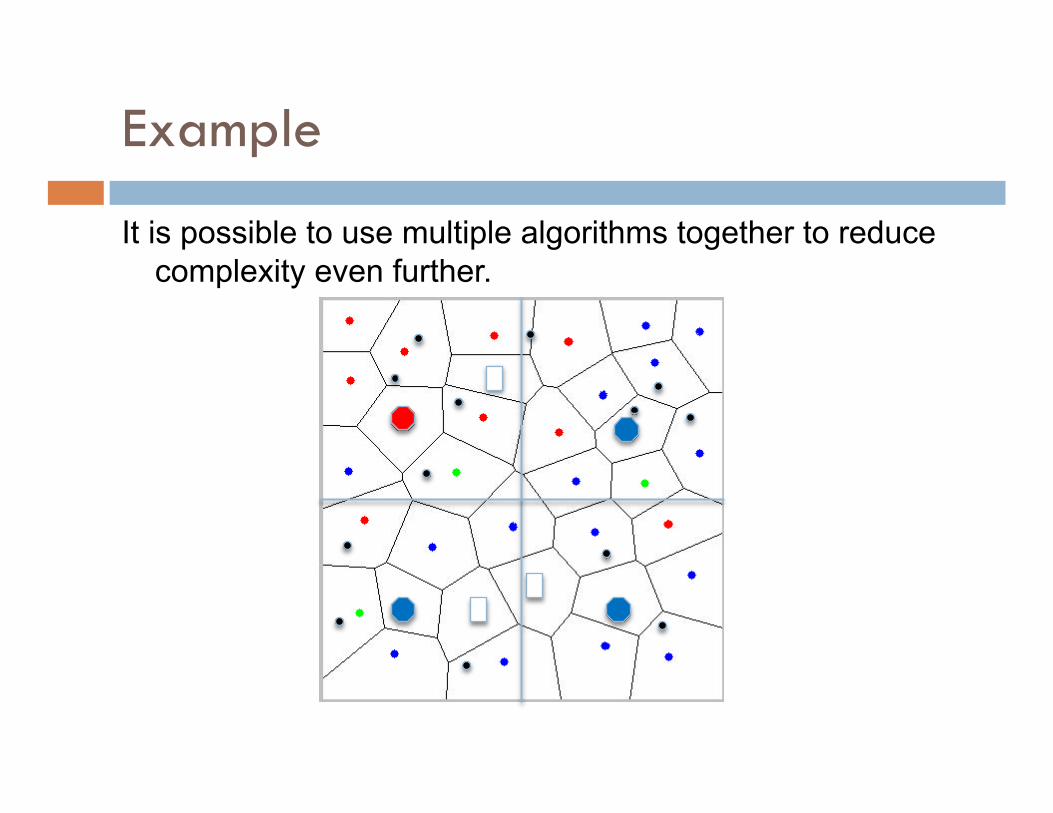
It is possible to use multiple algorithms together to reduce complexity even further.

k-Nearest Neighbor Using MaxNearestDist

Samet’s work expands depth-first search and best-first search algorithms.

His algorithms using the Max Nearest Distance as an upper bound can be shown to be no worse than the basic current algorithms while potentially being much faster.

k-Nearest Neighbor Using MaxNearestDist

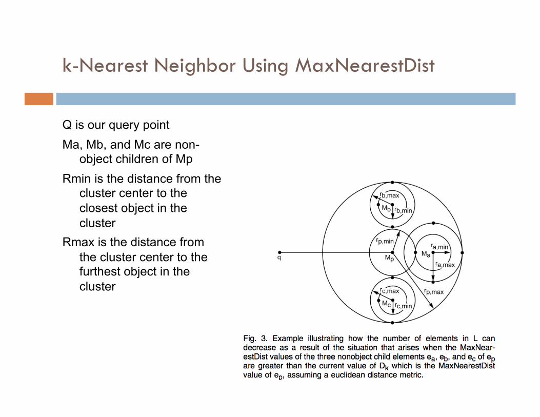
Q is our query point Ma, Mb, and Mc are non-

object children of Mp Rmin is the distance from the

cluster center to the closest object in the cluster

Rmax is the distance from the cluster center to the furthest object in the cluster

k-Nearest Neighbor Using MaxNearestDist

References

Samet, H., 2008. K-Nearest Neighbor Finding Using MaxNearestDist. IEEE Trans. Pattern Anal. Mach. Intell. 30, 2 (Feb. 2008), 243-252.

Duda, R., Hart, P., Stork, D., 2001. Pattern Classification, 2nd ed. John Wiley & Sons.

Yu-Long Qiao, Jeng-Shyang Pan, Sheng-He Sun .Improved partial distance search for k nearest-neighbor classification. IEEE International Conference on Multimedia and Expo, 2004. June 2004, 1275 - 1278