EART

H,A

TMO

SPH

ERIC

,A

ND

PLA

NET

ARY

SCIE

NCE

S

Network analysis reveals strongly localized impactsof El NinoJingfang Fana,1, Jun Menga,b,1, Yosef Ashkenazyb,2, Shlomo Havlina, and Hans Joachim Schellnhuberc,d,2

aDepartment of Physics, Bar-Ilan University, Ramat-Gan 52900, Israel; bDepartment of Solar Energy & Environmental Physics, Blaustein Institutes for DesertResearch, Ben-Gurion University of the Negev, Midreshet Ben-Gurion 84990, Israel; cPotsdam Institute for Climate Impact Research, 14412 Potsdam,Germany; and dSanta Fe Institute, Santa Fe, NM 87501

Contributed by Hans Joachim Schellnhuber, June 1, 2017 (sent for review January 23, 2017; reviewed by Dirk Helbing and Yochanan Kushnir)

Climatic conditions influence the culture and economy of soci-eties and the performance of economies. Specifically, El Nino as anextreme climate event is known to have notable effects on health,agriculture, industry, and conflict. Here, we construct directed andweighted climate networks based on near-surface air temperatureto investigate the global impacts of El Nino and La Nina. We findthat regions that are characterized by higher positive/negativenetwork “in”-weighted links are exhibiting stronger correlationswith the El Nino basin and are warmer/cooler during El Nino/LaNina periods. In contrast to non-El Nino periods, these stronger in-weighted activities are found to be concentrated in very localizedareas, whereas a large fraction of the globe is not influenced bythe events. The regions of localized activity vary from one El Nino(La Nina) event to another; still, some El Nino (La Nina) events aremore similar to each other. We quantify this similarity using net-work community structure. The results and methodology reportedhere may be used to improve the understanding and prediction ofEl Nino/La Nina events and also may be applied in the investiga-tion of other climate variables.

climate | dynamic network | ENSO

More than a decade ago, networks became the standardframework for studying complex systems (1–5). In recent

years, network theory has been implemented in climate sciencesto construct “climate networks.” These networks have been usedsuccessfully to analyze, model, understand, and even predict cli-mate phenomena (6–16). Specific examples of climate networkstudies include the investigation of the interaction structure ofcoupled climate subnetworks (17), the multiscale dependencewithin and among climate variables (18), the temporal evolutionand teleconnections of the North Atlantic Oscillation (19, 20),the finding of the dominant imprint of Rossby waves (21), theoptimal paths of teleconnection (22), the influence of El Nino onremote regions (8, 23, 24), the distinction of different types of ElNino events (25), and the prediction of these events (15, 16). Anetwork is composed of nodes and links; in a climate network,the nodes are the geographical locations, and the links are thecorrelations between them. The “strength” of the links is quan-tified according to the strength of the correlations between thedifferent nodes (21, 26, 27).

El Nino is probably the strongest climate phenomenon thatoccurs on interannual time scales (28, 29). El Nino refers to thewarming of the central and eastern equatorial Pacific Ocean byseveral degrees (◦C). La Nina is the cooling of sea surface tem-peratures (SSTs) in the eastern tropical Pacific Ocean. La Ninausually follows an El Nino event, but not always; the overall phe-nomenon is referred to as El Nino-Southern Oscillation (ENSO).This cycle occurs every 3–5 y with different magnitudes. Thereare several indices that quantify the El Nino activity, includingthe Nino 3.4 Index, the Southern Oscillation Index (SOI) (see,e.g., ref. 30), and the Oceanic Nino Index (ONI), which is theNational Oceanic and Atmospheric Administration’s (NOAA)primary indicator for monitoring El Nino and La Nina. ONI isthe running 3-mo mean SST anomaly for the Nino 3.4 region(i.e., 5◦N − 5◦S , 120◦− 170◦W ); here, we refer to this region as

the El Nino Basin (ENB). When the ONI is >0.5◦C for at leastfive consecutive months, the corresponding year is considered tobe an El Nino year. The higher the ONI is, the stronger the ElNino. Similarly, La Nina is determined to occur when the ONIdrops below the −0.5◦C anomaly for at least five consecutivemonths. Presently, we have just undergone one of the strongestEl Nino events since 1948 (31, 32).

The El Nino phenomenon strongly affects human life. It canlead to warming, enhanced rain in some regions and droughtsin other regions (33), decline in fishery, famine, plagues, evenincreases in the risks of political and social unrest, and economicchanges through globally networked system (34). Global maps ofthe influence of El Nino had been constructed in ref. 35. The cli-mate network approach has been found to be useful in improvingour understanding of El Nino (8, 23–25) and in forecasting it (15,16). However, that approach has not been developed and appliedto study systematically the global impact of El Nino, and that iswhat we try to achieve in quantitative terms here. We constructthe climate network by using only directed links from the ENBto regions outside the ENB (which we call here “in”-links). Theconstructed in-weighted climate network enables us not only toobtain a map of the global impacts of a given El Nino event, butalso to study the impacts of El Nino in specific regions, includingNorth America (36), Australia (37–41), South Africa (42), south-ern South America (43), Europe (44), and the tropical NorthAtlantic (45).

In the present study, we identify warming and cooling regionsthat are influenced by the ENB by measuring each node’sstrength according to the weights of its links “coming” fromthe ENB. We find that during El Nino/La Nina, a large frac-tion of the globe is not influenced by the events, but the regionsthat are influenced are significantly more affected by the ENBthan in normal years. Our findings support the recent sugges-

Significance

El Nino, one of the strongest climatic phenomena on interan-nual time scales, affects the climate system and is associatedwith natural disasters and serious social conflicts. Here, usingnetwork theory, we construct a directed and weighted climatenetwork to study the global impacts of El Nino and La Nina.The constructed climate network enables the identification ofthe regions that are most drastically affected by specific ElNino/La Nina events. Our analysis indicates that the effect ofthe El Nino basin on worldwide regions is more localized andstronger during El Nino events compared with normal times.

Author contributions: Y.A., S.H., and H.J.S. designed research; J.F. and J.M. performedresearch; J.F. and J.M. analyzed data; and J.F., J.M., Y.A., S.H., and H.J.S. wrote the paper.

Reviewers: D.H., ETH Zurich; and Y.K., Columbia University.

The authors declare no conflict of interest.1J.F. and J.M. contributed equally to this work.2To whom correspondence may be addressed. Email: ashkena@bgu.ac.il or john@pik-potsdam.de.

This article contains supporting information online at www.pnas.org/lookup/suppl/doi:10.1073/pnas.1701214114/-/DCSupplemental.

www.pnas.org/cgi/doi/10.1073/pnas.1701214114 PNAS | July 18, 2017 | vol. 114 | no. 29 | 7543–7548

Dow

nloa

ded

by g

uest

on

Apr

il 9,

202

0

tion that the climate structure becomes well-confined in certainlocalized regions during a fully developed El Nino event. Thisphenomenon is evident by inspecting the emergent teleconnec-tions between the ENB and localized regions. Such a large-scalecooperative mode helps us to forecast El Nino events (15, 16).Our results also indicate that the El Nino/La Nina events influ-ence different regions with different magnitudes during differentevents; still, by determining the network community structure,our results suggest that similarities exist among some of the ElNino (La Nina) events. We find here that the impact of El Ninois very variable and that it is localized and strong during El Ninoevents; we quantify this variability and the intensity effect andfound, using a directed and weighted network, that it is stronglyrelated to El Nino.

Our evolving climate network is constructed from the globaldaily near-surface (1000 hPa) air temperature fields of theNational Center for Environmental Prediction/National Centerfor Atmospheric Research (NCEP/NCAR) reanalysis dataset(46); see the SI Appendix for the analysis and results based onthe European Center for Medium-Range Weather ForecastsInterim Reanalysis (ref. 47 and SI Appendix). The spatial (zonaland meridional) resolution of the data are 2.5◦× 2.5◦, result-ing in 144× 73 = 10512 grid points. The dataset spans the timeperiod between January 1948 and April 2016. (Because for eachwindow 365 + 200 days’ daily data are used, and the newest datawe can obtain is until May 6, 2016, so Φy is terminated at the11th window of 2014.) To avoid the strong effect of seasonality,we subtract the mean seasonal cycle and divide by the seasonalSD for each grid point time series. The overall analysis is basedon a sequence of networks, each constructed from time seriesthat span 1 y.

The nodes (grid points) are divided into two subsets. Onesubset includes the nodes within the ENB (57 nodes) and theother the nodes outside the ENB (10455 nodes). For each pairof nodes, i and j , each from a different subset, respectively,the cross-correlation between the two time series of 365 d iscalculated,

C yi,j (τ) =

〈Ti(d)Tj (d − τ)〉 − 〈Ti(d)〉〈Tj (d − τ)〉σTi (d)σTj (d−τ)

, [1]

where σTi (d) is the SD of Ti(d), τ ∈ [0, τmax ] is the time lag, withτmax = 200 d, y indicates the starting date of the time series with0 time shift, and C y

i,j (−τ)≡C yj ,i(τ). We then identify the value

of the highest peak of the absolute value of the cross-correlationfunction and denote the corresponding time lag of this peak asθyi,j . The sign of θyi,j indicates the direction of each link; that is,when the time lag is positive (θyi,j > 0), the direction of the linkis from i to j . Below, we focus on the overall effect of the ENBon regions (grid points) outside this region and thus refer to thelinks directed from the ENB to a grid point j as in-links to gridpoint j (24). We only consider in-links with time lag shorter than∼5 mo (|θyi,j | ≤ 150 d) as we focus on the influence of El Ninoon the rest of the world on seasonal time scales. Examples ofin-links over different regions are shown in Fig. 1 A and B, andthe cross-correlation function of these typical links are presentedin SI Appendix, Fig. S4. Below, we elaborate on the impacts ofEl Nino in some of these regions. The link weights are deter-mined by using C y

i,j (θ), and we define the strength of thelink as

W yi,j =

C yi,j (θ)−mean(C y

i,j (τ))

std(C yi,j (τ))

, [2]

where “mean” and “std” are the mean and SD of the cross-correlation function, respectively (21, 22). We construct net-works based on both C y

i,j (θ) and W yi,j , and these are consistent

with each other. See Fig. 1 A and C for El Nino and Fig. 1 B andD for La Nina (details are below).

A

C D

FE

B

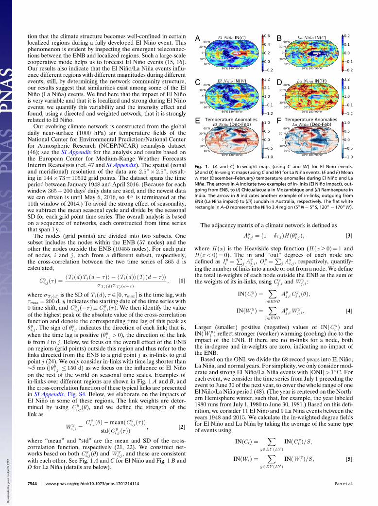
Fig. 1. (A and C) In-weight maps (using C and W) for El Nino events.(B and D) In-weight maps (using C and W) for La Nina events. (E and F) Meanwinter (December–February) temperature anomalies during El Nino and LaNina. The arrows in A indicate two examples of in-links (El Nino impact), out-going from ENB, to (i) Chicualacuala in Mozambique and (ii) Rambaxpura inIndia. The arrow in B indicates another example of in-links, outgoing fromENB (La Nina impact) to (iii) Jundah in Australia, respectively. The flat whiterectangle in A–D represents the Nino 3.4 region (5◦N−5◦S, 120◦−170◦W).

The adjacency matrix of a climate network is defined as

Ayi,j = (1− δi,j )H (θyi,j ), [3]

where H (x ) is the Heaviside step function (H (x ≥ 0) = 1 andH (x < 0) = 0). The in and “out” degrees of each node aredefined as I y

i =∑

j Ayj ,i , O

yi =

∑j A

yi,j , respectively, quantify-

ing the number of links into a node or out from a node. We definethe total in-weights of each node outside the ENB as the sum ofthe weights of its in-links, using C y

j ,i and W yj ,i :

IN(C yi ) =

∑j∈ENB

Ayj ,iC

yj ,i(θ),

IN(W yi ) =

∑j∈ENB

Ayj ,iW

yj ,i . [4]

Larger (smaller) positive (negative) values of IN(C yi ) and

IN(W yi ) reflect stronger (weaker) warming (cooling) due to the

impact of the ENB. If there are no in-links for a node, boththe in-degree and in-weights are zero, indicating no impact ofthe ENB.

Based on the ONI, we divide the 68 record years into El Nino,La Nina, and normal years. For simplicity, we only consider mod-erate and strong El Nino/La Nina events with |ONI|> 1◦C. Foreach event, we consider the time series from July 1 preceding theevent to June 30 of the next year, to cover the whole range of oneEl Nino/La Nina period (48). (The year is centered on the North-ern Hemisphere winter, such that, for example, the year labeled1980 runs from July 1, 1980 to June 30, 1981.) Based on this defi-nition, we consider 11 El Nino and 9 La Nina events between theyears 1948 and 2015. We calculate the in-weighted degree fieldsfor El Nino and La Nina by taking the average of the same typeof events using

IN(Ci) =∑

y∈EY (LY )

IN(C yi )/S ,

IN(Wi) =∑

y∈EY (LY )

IN(W yi )/S , [5]

7544 | www.pnas.org/cgi/doi/10.1073/pnas.1701214114 Fan et al.

Dow

nloa

ded

by g

uest

on

Apr

il 9,

202

0

EART

H,A

TMO

SPH

ERIC

,A

ND

PLA

NET

ARY

SCIE

NCE

S

where S =∑

y∈EY (LY )

I yi , and EY and LY refer to the years (as

defined above) in which El Nino and La Nina occur, respectively.It is seen that regions affected by El Nino/La Nina, either by

warming or cooling, such as North America (49), South Amer-ica (50), Europe (51), India (52), South Africa (53, 54), andAustralia (39), are characterized by relatively high in-weights(Fig. 1 A–D) and by high temperature anomalies (Fig. 1 E andF). The maps of temperature anomalies in Fig. 1 E and F areobtained by first calculating a 3-mo (December–February) meantemperature anomaly for each year, and then taking an averageof the mean value over all El Nino/La Nina years. The El Nino/LaNina-related in-weighted extent fields are hemispherically sym-metric, to some degree, in accordance with refs. 48 and 55.

In Table 1, we compare the in-weighted degree maps ofEl Nino/La Nina events with the corresponding temperatureanomaly maps by evaluating the cross-correlation between eachpair of maps shown in Fig. 1. Note that the different grid pointsare weighted by the cosine of the latitude, to account for thelower weights (due to the smaller area) at the higher latitudes.The cross-correlation values are found to be high, indicating thesimilarity between the different measures. For more detail, seeSI Appendix, Tables S2 and S3. In addition, we also find that theaveraged effects of El Nino and La Nina on different regionsshown in Fig. 1 are quite similar. The cross-correlation valuebetween Fig. 1 A and B is 0.54, indicating that El Nino andLa Nina tend to affect similar regions.

Next, we study the variability of the regions that are influencedby El Nino/La Nina. We find that during El Nino/La Nina events,the overall global area that is influenced by the ENB becomessmaller, whereas the impacts in these more limited areas becomestronger. This enhanced impact in localized regions is demon-strated in Fig. 2, which compares the global distributions of thein-degrees, IN(N ); in-weights, IN(W ); and IN(C ), of typical ElNino and normal years. For IN(N ), the differences are quitedistinct—we see broader black regions (that indicate the absenceof in-links), as well as broader dark red regions (that indicatethat all links connected with the 57 grid points of the ENB arein-links), during El Nino years (Fig. 2A), compared with normalyears (Fig. 2B). The underlying reason for this contrast is that,during El Nino, the temperatures of all 57 nodes located in theENB are synchronized, such that for each influenced node out-side the ENB, the 57 links with the ENB are more likely to havethe same direction (i.e., outgoing from the ENB); this situationis less likely during normal years. We also find the localized phe-nomenon for in-weights, during El Nino years (Fig. 2 C and E),compared with normal years (Fig. 2 D and F). See also examplesof cross-correlation functions for nodes inside and outside theENB during El Nino in SI Appendix, Fig. S3.

A quantitative analysis of the area (number of nodes) that isaffected/unaffected during El Nino and La Nina years is shown inFig. 3, where El Nino and La Nina years are, respectively, empha-sized by the red and blue shading. Here, the temporal evolutionof the climate network is studied by constructing a sequence ofnetworks based on successive windows of lengths of 365 + 200 d,with a beginning date that is shifted by 1 mo each time. Fig. 3Adepicts the ONI as a function of time. We focus on El Nino

Table 1. Comparison (using cross-correlation) between thein-weighted degree fields and the El Nino/La Nina meanwinter temperature anomaly shown in Fig. 1

R El Nino La Nina

RIN(C),T 0.59 −0.55RIN(W),T 0.54 −0.51RIN(W),IN(C) 0.92 0.95

See SI Appendix, Eqs. S1–S3 in the for the definition of R.

A

C

E

D

F

B

Fig. 2. The in-degree fields (N, W, and C) in a typical El Nino event, 1972(A, C, and E), and a normal year, 1959 (B, D, and F).

(La Nina) events with ONIs that are larger (smaller) than 1◦C(−1◦C). Fig. 3B depicts the number of nodes with zero in-degreeN y as a function of time, and Fig. 3C depicts the average in-weights per node, which are given by dividing the sum of theabsolute weights of all in-links of each node outside the ENBby N y :

C y =∑

i /∈ENB

∑j∈ENB

Ayj ,i |C

yj ,i(θ)|/N

y . [6]

Fig. 3 shows the 3-mo running average of N y and C y .It actually is seen that, during El Nino/La Nina, the number of

nodes with no in-links, N y , drops dramatically (Fig. 3B), indicat-ing that the total area influenced by the ENB is much smaller.Moreover, during El Nino/La Nina, C y increases significantly(Fig. 3C), indicating a stronger impact of the ENB in the areasthat are influenced by it. We chose the 1982–1983 El Nino eventto depict the evolution of ENSO impact, from its onset to itsdecay. We plot the in-weight maps every 3 mo (SI Appendix,Fig. S12). We find that, during the El-Nino event, the links aremore localized in comparison with the beginning and the end ofthe event. To quantify the significance of the results, we used arandomization procedure in which we shuffled the years of eachnode’s time series (keeping the time ordering within each yearunchanged) and then constructed the in-weighted networks. Wefound that C y ≥ 8 and N y ≤ 6300 are significant with P values<10−3. Other related network quantities are summarized in SIAppendix, Figs. S5–S7 and Table S1. The success of the climate-network-based measures to detect the El Nino/La Nina eventsstrengthens the reliability of this approach in studying climatephenomenon.

It is possible to classify El Nino events based on the loca-tion of their maximum SST anomalies and on their tropicalmidlatitude teleconnections (56, 57). Here, we propose classi-fying different types of El Nino events based on the similaritybetween them, which can be determined by the cross-correlationsbetween pairs of maps. We determine the significance of thecross-correlation using shuffled network maps. The shuffling isperformed by dividing the map (globe) into 18 equal areas, shuf-fling their spatial orders for each event, and then evaluating thecross-correlation between each pair of the shuffled global net-work maps. Eventually, we obtain a distribution of the cross-correlation values through the shuffling process. Only correla-tions with P values <0.01 are considered as significant.

Fan et al. PNAS | July 18, 2017 | vol. 114 | no. 29 | 7545

Dow

nloa

ded

by g

uest

on

Apr

il 9,

202

0

A

B

C

Fig. 3. (A) The ONI as a function of time. (B) The evolution of the numberof nodes that have in-links with time. (C) The evolution of the average in-weights per node with time.

The cross-correlations between pairs of El Nino events isshown in Fig. 4A; insignificant cross-correlation is indicated bythe white color. Based on this heat map, the 11 El Nino eventsare divided into three groups with extended white areas separat-ing them, indicating that El Nino events within the same grouptend to have similar global impact patterns. Furthermore, wedivide the globe into three regions, approximately equal in area:“Tropics” (20◦S to 20◦N), “North” (20◦N to 90◦N), and “South”(20◦S to 90◦S). Then, separately for each region, we calculate thecross-correlations between the map pairs of the in-weighted cli-mate network. The significant cross-correlations are also deter-mined by P values<0.01, by shuffling the spatial orders of nodeswithin the same regions. The heat maps of cross-correlations forthe different regions are shown in Fig. 4 B–D. We find that theglobal similarity structure receives different contributions fromdifferent regions. More specifically, the heat map for the Tropicsregion (Fig. 4B) is much more similar to the heat map for theglobal area (Fig. 4A), in comparison with the other two regions,indicating that the impact of El Nino in the tropics dominates theclassification of El Nino events. We also construct the matrix ofsimilarity of El Nino events based on the mean winter tempera-ture anomaly and find that it is consistent with the network-basedsimilarity structure (SI Appendix, Fig. S9).

A weighted network of the 11 El Nino years is also constructedbased on the significant correlations given in Fig. 4A and is shownin Fig. 4E; the thickness of each link represents the correlationvalue between the two connected years. Then, by using a modu-larity optimization heuristic algorithm (58), our network is subdi-vided into three communities, which is consistent with the groupsin Fig. 4A. To view the correlation patterns associated with eachof the three communities, we chose three representative El Ninoyears (2009, 1986, and 1957), each from a different community.The in-weight maps are shown in SI Appendix, Fig. S11. The cor-relation patterns are quite different from each other; the corre-lation coefficients between them are summarized in Fig. 4A.

In summary, a general pattern of El Nino/La Nina’s globalimpacts, as well as of their dynamical evolutions, are obtainedfrom a time-evolving in-weighted climate network. By averag-ing the in-weighted degree fields of all significant El Nino/LaNina events, we identify the regions that tend to be more influ-enced by those events. One of the most important results of ourstudy is that, during El Nino/La Nina periods, a smaller worldarea is affected by the ENB, but the impact of El Nino/La Ninais enhanced in these more localized regions. This observation isrooted in the fact that, during El Nino/La Nina, the entire ENBwarms/cools; in addition, the regions that become warmer/cooler

have similar/opposite tendencies with respect to the ENB. Thesesynchronized behaviors enhance the overall correlation of theENB with the rest of the world. However, during normal peri-ods, part of the ENB is correlated and part is not, thus reducingthe overall correlation and extending the regions of correlation.

The method proposed above enables the detection of localeffects of each El Nino event; see SI Appendix, Fig. S10 for exam-ples of climate networks of several El Nino and La Nina events.Evidently, these enhanced and localized El Nino effects are asso-ciated with serious consequences in many aspects of human life(59–62). In Fig. 1 A and B, we indicate (by arrows) three exam-ples of regional effects of El Nino/La Nina discussed below.(i) Droughts and floods exacerbated by El Nino had directlyaffected East Africa, leading to an increase in food insecurityand malnutrition. El Nino had a varied significant impact onthis region, ranging from floods affecting >3.4 million peopleduring the 2006–2007 event to drought affecting >14 millionpeople during the 2009–2010 event. Excessive rains during the2014–2016 event have led to flooding in parts of Somalia, Kenya,Ethiopia, and Uganda, affecting nearly 410,000 people, displac-ing >231,900 people, and killing 271 people in the region (63).(ii) Agricultural output in India depends on the summer mon-soons that are influenced by the timing, location, and intensityof El Nino. Some droughts in India have been accompanied byEl Nino events (52). For example, the 2002–2003 El Nino eventwas accompanied by one of the worst Indian droughts in thepast century, decreased the agricultural (cotton, oilseeds, andsugarcane) output, and led to food inflation (64). (iii) Precip-itation in Australia had been associated with ENSO (38, 39),where El Nino (La Nina) tended to increase the risk of dry(wet) conditions across many parts of the continent (65). The2010–2012 La Nina event was particularly important because itled to flooding across Australia and to the termination of theparticular strong “Millennium Drought” (2001–2010) in easternAustralia (66).

The method we propose here enables the detection of theabove regions as well as other regions across the globe that areaffected by ENSO. See SI Appendix, Fig. S4 for typical cross-correlation functions during the specific El Nino events andregions described above.

The regions affected by El Nino vary from one El Nino eventto another, making it difficult to predict the impacts of an upcom-ing El Nino. However, it is still possible to evaluate for eachregion (grid point) the probability to be affected by ENB by using

Fig. 4. The community structure of the 11 El Nino events. (A–D) The heatmap of cross-correlations between pairs of El Nino events, based on theglobal (A), tropical (B), Northern Hemisphere (C), and Southern Hemisphere(D) maps of the in-weighted climate network. (E) Community structurein the network of 11 El Nino events. Different colors represent differentcommunities.

7546 | www.pnas.org/cgi/doi/10.1073/pnas.1701214114 Fan et al.

Dow

nloa

ded

by g

uest

on

Apr

il 9,

202

0

EART

H,A

TMO

SPH

ERIC

,A

ND

PLA

NET

ARY

SCIE

NCE

S

our climate network approach. We define the frequency Pi foreach node i in which the in-degrees I y

i are nonzero. This Pi

quantifies the probability effected by ENB. SI Appendix, Fig.S13 shows the spatial distribution of Pi ≥ 10 (among 11 El Ninoevents); these regions are marked by red color (indicating proba-bility>> 90%) and include Australia (37–41), South Africa (42),southern South America (43), and Europe (44). El Nino phe-nomena can lead to warming or cooling in some regions, andthe warming or cooling can be quantified by using IN(C y

i )–positive values for warming effects and negative values for cool-ing effects. SI Appendix, Fig. S14 A and B shows the spa-tial distribution of positive and negative IN(C y

i ) frequency,respectively. We find that some regions, such as Western NorthAmerican, Western South America, South Indian, South Africa,and South Pacific, are very frequently and positively (warm-ing) affected by El Nino; yet some regions, such as South-ern South America and North Asian, are very frequently andnegatively (cooling) affected (SI Appendix, Fig. S14). Theseresults are consistent to some degree with the temperatureanomalies during El Nino shown in Fig. 1E. To strengthen theabove results, we also analyzed the frequency (during El Ninoyears) of the temperature anomalies to be above or belowone SD of normal years (SI Appendix, Fig. S14 C and D).These results support the results obtained by using the networkapproach (compare SI Appendix, Fig. S14 A–C for warming andSI Appendix, Fig. S14 B–D for cooling) and can help to identifythe regions that have the highest probability to be affected byEl Nino.

Finally, according to our results, different El Nino events candrive different extreme weather conditions in different regions.For instance, the recently terminated El Nino event was dis-tinct from most El Nino events in certain key aspects of cli-mate disruptions (32). Collecting updated information is impor-tant in improving related models. Meanwhile, the detection ofsimilarities between different El Nino events is also helpfulin understanding important common aspects. We distinguishbetween different types of El Nino events based on the simi-larities between the networks of these events. According to ourresults, the similarities between different events are mostly dueto the impacts of El Nino on Tropics (20◦S to 20◦N) comparedwith North (20◦N to 90◦N) and South (20◦S to 90◦S); the Trop-ics area is ∼1/3 of the global world area. The methodology andresults presented here may help to improve the understanding ofthe impacts of ENSO, and hopefully to provide the ability, in thefuture, to take early actions to reduce the damage caused by ElNino. The mechanism underlying the results reported above isstill not clear to us, and further study, maybe related to telecon-nections, is needed to explore this mechanism.

ACKNOWLEDGMENTS. We thank Avi Gozolchiani for helpful discussions.This work was supported by MULTIPLEX EU (European Union) Project317532; the Israel Science Foundation; the Israel Ministry of Science andTechnology (MOST) with the Italy Ministry of Foreign Affairs; MOST with theJapan Science and Technology Agency; the Office of Naval Research; andthe Defense Threat Reduction Agency. J.F. was supported by a fellowshipprogram funded by the Planning and Budgeting Committee of the Councilfor Higher Education of Israel.

1. Watts D, Strogatz S (1998) Collective dynamics of ‘small-world’ networks. Nature393:440–442.

2. Barabasi A, Albert R (1999) Emergence of scaling in random networks. Science286:509–512.

3. Brockmann D, Helbing D (2013) The hidden geometry of complex, network-drivencontagion phenomena. Science 342:1337–1342.

4. Cohen R, Havlin S (2010) Complex Networks: Structure, Robustness and Function(Cambridge Univ Press, Cambridge, UK).

5. Newman M (2010) Networks: An Introduction (Oxford Univ Press, New York).6. Tsonis AA, Swanson KL, Roebber PJ (2006) What do networks have to do with climate?

Bull Am Meteorol Soc 87:585–595.7. Tsonis AA, Swanson KL, Kravtsov S (2007) A new dynamical mechanism for major

climate shifts. Geophys Res Lett 34:L13705.8. Yamasaki K, Gozolchiani A, Havlin S (2008) Climate networks around the globe are

significantly affected by El Nino. Phys Rev Lett 100:228501.9. Donges JF, Zou Y, Marvan N, Kurths J (2009) Complex networks in climate dynamics.

Eur Phys J Spec Top 174:157–179.10. Donges JF, Zou Y, Marvan N, Kurths J (2009) The backbone of the climate network.

Europhys Lett 87:48007.11. Steinhaeuser K, Chawla NV, Ganguly AR (2010) An exploration of climate data using

complex networks. SIGKDD Explor 12:25–32.12. Steinhaeuser K, Chawla NV, Ganguly AR (2011) Complex networks as a unified frame-

work for descriptive analysis and predictive modeling in climate science. Statist AnalData Min 4:497–511.

13. Barreiro M, Marti AC, Masoller C (2011) Inferring long memory processes in the cli-mate network via ordinal pattern analysis. Chaos 21:013101.

14. Deza J, Barreiro M, Masoller C (2013) Inferring interdependencies in climate networksconstructed at inter-annual, intra-season and longer time scales. Eur Phys J Spec Top222:511–523.

15. Ludescher J, et al. (2013) Improved El Nino forecasting by cooperativity detection.Proc Natl Acad Sci USA 110:11742–11745.

16. Ludescher J, et al. (2014) Very early warning of next El Nino. Proc Natl Acad Sci USA111:2064–2066.

17. Donges JF, Schultz HCH, Marwan N, Zou Y, Kurths J (2011) Investigating the topologyof interacting networks. Eur Phys J B 84:635–651.

18. Steinhaeuser K, Ganguly AR, Chawla NV (2012) Multivariate and multiscale depen-dence in the global climate system revealed through complex networks. Clim Dynam39:889–895.

19. Guez O, Gozolchiani A, Berezin Y, Brenner S, Havlin S (2012) Climate net-work structure evolves with North Atlantic oscillation phases. Europhys Lett 98:38006.

20. Guez O, Gozolchiani A, Berezin Y, Wang Y, Havlin S (2013) Global climate networkevolves with North Atlantic Oscillation phases: Coupling to Southern Pacific Ocean.Europhys Lett 103:68006.

21. Wang Y, et al. (2013) Dominant imprint of Rossby waves in the climate network. PhysRev Lett 111:138501.

22. Zhou D, Gozolchiani A, Ashkenazy Y, Havlin S (2015) Teleconnection paths via climatenetwork direct link detection. Phys Rev Lett 115:268501.

23. Tsonis AA, Swanson KL (2008) Topology and predictability of El Nino and La Ninanetworks. Phys Rev Lett 100:228502.

24. Gozolchiani A, Havlin S, Yamasaki K (2011) Emergence of El Nino as an autonomouscomponent in the climate network. Phys Rev Lett 107:148501.

25. Radebach A, Donner RV, Runge J, Donges JF, Kurths J (2013) Disentangling differenttypes of El Nino episodes by evolving climate network analysis. Phys Rev E 88:052807.

26. Barrat A, Barthelemy M, Pastor-Satorras R, Vespignani A (2004) The architecture ofcomplex weighted networks. Proc Natl Acad Sci USA 101:3747–3752.

27. Zemp DC, Wiedermann M, Kurths J, Rammig A, Donges JF (2014) Node-weightedmeasures for complex networks with directed and weighted edges for studying con-tinental moisture recycling. Europhys Lett 107:58005.

28. Sarachik ES, Cane MA (2010 The El Nino-Southern Oscillation Phenomenon(Cambridge Univ Press, Cambridge, UK).

29. Dijkstra HA (2005) Nonlinear Physical Oceanography: A Dynamical Systems Approachto the Large Scale Ocean Circulation and El Nino (Springer Science, New York).

30. Dijkstra HA (2006) The ENSO phenomenon: Theory and mechanisms. Adv Geosci 6:3–15.

31. Levine AFZ, McPhaden MJ (2016) How the July 2014 easterly wind burst gave the2015-2016 El Nino a head start. Geophys Res Lett 43:6503–6510.

32. Kintisch E (2016) How a ‘Godzilla’ El Nino shook up weather forecasts. Science352:1501–1502.

33. Giannini A, Chiang J, Cane MA, Kushnir Y, Seager R (2001) The ENSO teleconnectionto the tropical Atlantic Ocean: Contributions of the remote and local SSTs to rainfallvariability in the tropical Americas. J Clim 14:4530–4544.

34. Helbing D (2013) Globally networked risks and how to respond. Nature 497:51–59.35. Halpert MS, Ropelewski CF (1992) Surface temperature patterns associated with the

Southern Oscillation. J Clim 5:577–593.36. Ropelewski CF, Halpert MS (1986) North American precipitation and temperature

patterns associated with the El Nino/Southern Oscillation (ENSO). Mon Weather Rev114:2352–2362.

37. Chiew FHS, Piechota TC, Dracup JA, McMahon TA (1998) El Nino/Southern Oscillationand Australian rainfall, streamflow and drought: Links and potential for forecasting.J Hydrol 204:138–149.

38. Power S, et al. (1999) Australian temperature, Australian rainfall and the SouthernOscillation, 1910-1992: Coherent variability and recent changes. Aust Meteorol Mag47:85–101.

39. Power S, Casey T, Folland C, Colman A, Mehta V (1999) Inter-decadal modulation ofthe impact of ENSO on Australia. Clim Dynam 15:319–324.

40. Wang G, Hendon HH (2007) Sensitivity of Australian rainfall to inter-El Nino varia-tions. J Clim 20:4211–4226.

41. Taschetto AS, England MH (2009) El Nino Modoki impacts on Australian rainfall.J Clim 22:3167–3174.

42. Reason CJC, Jagadheesha D (2005) A model investigation of recent ENSO impacts overSouthern Africa. Meteorol Atmos Phys 89:181–205.

Fan et al. PNAS | July 18, 2017 | vol. 114 | no. 29 | 7547

Dow

nloa

ded

by g

uest

on

Apr

il 9,

202

0

43. Magana V, Ambrizzi T (2005) Dynamics of subtropical vertical motions over the Amer-icas during El Nino boreal winters. Atmosfera 18:211–235.

44. Bronnimann S (2007) Impact of El Nino–Southern Oscillation on European climate.Rev Geophys 45:RG3003.

45. Klein SA, Soden BJ, Lau NC (1999) Remote sea surface temperature varia-tions during ENSO: Evidence for a tropical atmospheric bridge. J Clim 12:917–932.

46. Kalnay E, et al. (1996) The NCEP/NCAR 40-year reanalysis project. Bull Am MeteorolSoc 77:437–471.

47. Dee DP, et al. (2011) The ERA-Interim reanalysis: Configuration and performance ofthe data assimilation system. Q J R Meteorol Soc 137:553–597.

48. Seager R, Harnik N, Kushnir Y (2003) Mechanisms of hemispherically symmetric cli-mate variability. J Clim 16:2960–2978.

49. Cane MA (1998) A role for the tropical Pacific. Science 282:59–61.50. Grimm AM, Barros VR, Doyle ME (2000) Climate variability in southern South America

associated with El Nino and La Nina events. J Clim 13:35–58.51. Fraedrich K, Muller K (1992) Climate anomalies in Europe associated with ENSO

extremes. Int J Climatol 12:25–31.52. Kumar KK, Rajagopalan B, Hoerling M, Bates G, Cane M (2006) Unravel-

ing the mystery of Indian monsoon failure during El Nino. Science 314:115–119.

53. Baylis M, Mellor PS, Meiswinkel R (1999) Horse sickness and ENSO in South Africa.Nature 397:574–574.

54. Anyamba A, Tucker CJ, Mahoney R (2002) From El Nino to La Nina: Vegetationresponse patterns over East and Southern Africa during the 1997-2000 period. J Clim15:3096–3103.

55. Seager R, et al. (2005) Mechanisms of ENSO-forcing of hemispherically symmetric pre-cipitation variability. Q J R Meteorol Soc 131:1501–1527.

56. Ashok K, Behera SK, Rao SA, Weng H, Yamagata T (2007) El Nino Modoki and itspossible teleconnection. J Geophys Res 112:C11007 .

57. Yeh SW, et al. (2009) El Nino in a changing climate. Nature 461:511–514.58. Blondel VD, Guillaume JL, Lambiotte R, Lefebvre E (2008) Fast unfolding of commu-

nities in large networks. J Stat Mech 2008:P10008.59. Hsiang SM, Meng KC, Cane MA (2011) Civil conflicts are associated with the global

climate. Nature 476:438–441.60. Schleussner CF, Donges JF, Donner RV, Schellnhuber HJ (2016) Armed-conflict risks

enhanced by climate-related disasters in ethnically fractionalized countries. Proc NatlAcad Sci USA 113:9216–9221.

61. Burke M, Gong E, Jones K (2015) Income shocks and HIV in Africa. Econ J 125:1157–1189.

62. Currie J, Rossin SM (2013) Weathering the storm: Hurricanes and birth outcomes.J Health Econ 32:487–503.

63. World Health Organization (2017) Emergency Events Database (EM-DAT) of theWorld Health Organization. Available at www.unocha.org/legacy/el-nino-east-africa.Accessed January 21, 2017.

64. Gadgil S, Rajeevan M, Nanjundiah R (2005) Monsoon prediction-why yet another fail-ure? Curr Sci 88:1389–1400.

65. Power S, Haylock M, Colman R, Wang X (2006) The predictability of interdecadalchanges in ENSO activity and ENSO teleconnections. J Clim 19:4755–4771.

66. Gergis J, et al. (2012) On the long-term context of the 1997–2009 ‘Big Dry’in South-Eastern Australia: Insights from a 206-year multi-proxy rainfall reconstruction. ClimChange 111:923–944.

7548 | www.pnas.org/cgi/doi/10.1073/pnas.1701214114 Fan et al.

Dow

nloa

ded

by g

uest

on

Apr

il 9,

202

0