network dea: a slacks-based measure approach policy information center discussion paper: 07-08 1...
TRANSCRIPT

GRIPS Policy Information Center Discussion Paper: 07-08
1
Network DEA: A slacks-based measure approach☆
Kaoru Tone*a and Miki Tsutsuib
aNational Graduate Institute for Policy Studies, 7-22-1 Roppongi, Minato-ku, Tokyo 106-8677, Japan
bCentral Research Institute of Electric Power Industry, 2-11-1 Iwado Kita, Komae-shi,
Tokyo 201-8511, Japan
Abstract
Traditional DEA models deal with measurements of relative efficiency of DMUs regarding multiple-inputs vs. multiple-outputs. One of the drawbacks of these models is the neglect of intermediate products or linking activities. After pointing out needs for inclusion of them in DEA models, we propose a slacks-based network DEA model that can deal with intermediate products. Using this model we can evaluate divisional efficiencies along with the overall efficiency of decision making units (DMUs).
Keyword: Data envelopment analysis, Network DEA, SBM, divisional efficiency, overall efficiency
1. Introduction Traditional DEA models deal with measurements of relative efficiency of DMUs
regarding multiple-inputs vs. multiple-outputs. One of the drawbacks of these models is the neglect of internal or linking activities. For example, many companies are comprised of several divisions that are linked as illustrated in Figure 1. In the example, the company has three divisions. Each division utilizes its own input resources for producing its own outputs. However, there are linking activities (or intermediate products) as shown by Link 1→2, Link 1→3 and Link 2→3. Link 1→2 indicates that part of the outputs from Division 1 are utilized as inputs to Division 2. In traditional DEA models, every activity should belong to either an input or an output but not to both. Thus, these models cannot deal with intermediate products formally.
<Figure 1: Company with three linked divisions>
☆ This research is fully supported by Grant-in-Aid for Scientific Research (B) Japan
Society for the Promotion of Science. * Corresponding author. Fax +81-3-6439-6010. E-mail address: [email protected]

GRIPS Policy Information Center Discussion Paper: 07-08
2
Although there may be many variants of this process flow, the existence of linking activities is an indispensable part of Network DEA models.
Within traditional DEA models there are at least two approaches for evaluating the efficiency of multi-division organizations.
1.1 Aggregation (Black box)
A simple approach is to aggregate these divisions into a single company which utilizes Inputs 1, 2 and 3, and produces Outputs 1, 2 and 3 (Figure 2). However, using this approach we neglect internal linking activities, and thus, we cannot evaluate the impact of division-specific inefficiencies on the overall efficiency of the company as a whole. In other words, the analysis does not fully access the underlying diagnostic value potentially available to management.
<Figure 2: Aggregation>
1.2 Separation The second approach is to evaluate divisional efficiency individually. In this case, we
evaluate the efficiency of Division 1 of each company among the set of DMUs using Input 1, and Output 1, Link 1→2 and Link 1→3 as outputs. Similarly we evaluate the efficiency of Division 2 of each company among the set of DMUs using Link 1→2 and Input 2 as inputs, and Link 2→3 and Output 2 as outputs. In this way, we can evaluate efficiency of each division of a company among the set of DMUs, and hence can find benchmarks for each division. However, this approach does not account for the continuity of links between divisions.
<Figure 3: Separation>
1.3 Needs for Network DEA The above observations lead us to consider a DEA model called “Network DEA
(NDEA) model” that accounts for divisional efficiencies as well as the overall efficiency in a unified framework. Network DEA models were introduced in the innovative book [6] by Färe and Grosskopf (see also [5, 7]). They investigated the so-called “black box” for the first time. Their models were extended by several authors. The network DEA model [10] proposed by Lewis and Sexton has a multi-stage structure as an extension of the two-stage DEA model proposed in Sexton and Lewis [15]. This study solves a DEA

GRIPS Policy Information Center Discussion Paper: 07-08
3
model for each node independently. For an output-oriented model, firstly a general DEA model is solved for the upstream node at the 1st stage to obtain the optimal solution of outputs. At the next stage, a part of (or all of) optimal outputs obtained at the upstream node are applied as intermediate inputs to the next node. After solving DEA models for all nodes in turn, a final optimal output is obtained at the last node. The firm-level efficiency score is measured as the final optimal output divided by an observed output. Prieto and Zofio [13] applied network efficiency analysis within an input-output model initiated by Koopmans [9]. They optimized primary input allocations, intermediate products and final demand products by way of Network DEA techniques and succeeded in applying their models to input-output database of OECD countries. Löthgren and Tambour [11] applied Network DEA model to a sample of Swedish pharmacies with organizational objectives that necessitates a monitoring of efficiency and productivity as well as customer satisfaction. They compared the results of Network DEA models with those of traditional DEA models.
The above Network DEA models utilize the radial measure of efficiency, e.g. the CCR (Charnes et al. [3]) or the BCC (Banker et al. [2]) models as the basic DEA methodology and the production possibility set. The radial models stand on the assumption that inputs or outputs undergo proportional changes. However, this assumption needs care. For example, if we employ labor, materials and capital as inputs, some of them are substitutional and do not change proportionally.
This current article introduces a network DEA model but uses the slacks-based measure (SBM: Tone [16], Pastor et al. [12] ) approach for evaluating efficiency. The SBM is a non-radial method and is suitable for measuring efficiencies when inputs and outputs may change non-proportionally. This model can decompose the overall efficiency into divisional ones. Furthermore, we employ the weighted SBM model (Cooper et al. [4], Tsutsui and Goto [18]) in order to incorporate the importance of divisions into account. We also investigate several properties of NDEA models and show that, under the variable returns-to-scale assumption, every division has at least one efficient DMU (decision making unit) for the division, whereas under the constant returns-to-scale assumption it is possible that some division has no efficient DMUs for the division.
The remainder of this paper unfolds as follows. In the next section, we introduce several network structures in actual business situations. Then in Section 3, we propose Network DEA (NDEA) models based on the weighted slacks-based measure (WSBM) approach. We discuss several characteristics of NDEA including divisional efficiencies in Section 4. Illustrative examples are introduced in Section 5. We extend our models in Section 6. We summarize the results and conclude the paper in the last section. Finally,

GRIPS Policy Information Center Discussion Paper: 07-08
4
in the Appendix, we propose a scheme for transforming non-positive data into positive data. Since the proposed NDEA models can deal only with positive data, this transformation is a necessity.
2. Several examples of network structures
Below, we introduce network structures from actual businesses that motivated this study.
2.1 Electric power companies
Figure 4 exhibits typical vertically integrated electric utility companies consisting of Generation, Transmission and Distribution divisions.
The generation division (Division 1) uses several inputs such as capital, labor and fuel (Input 1) and produces electric power. Then it becomes an intermediate input for the transmission division (Link1-2). In the transmission division (Division 2), companies utilize capital and labor inputs (Input 2) as well as the intermediate inputs from generation division (Link1-2). Electricity through transmission lines is sent to distribution division as intermediate output (Link 2-3) or sales to large customers (Output 2) that do not utilize distribution line. The distribution division (Division 3) uses capital and labor inputs (Input 3) and the intermediate input from the transmission division (Link 2-3) and provides electricity to small customers (Output 3).
<Figure 4: Vertically integrated electric power companies>
2.2 Hospitals Kaihara et al. [8] report the standard structure of Japanese general hospitals as
depicted in Figure 5. A general hospital consists of divisions, such as medical department, clinical laboratory, radiology, pharmacy and dietetic department. Each division has its own inputs; labor, materials and capital, and outputs; incomes. These divisions are connected by internal links. For example, a part of patients checked up at medical department is sent to radiology department. In order to evaluate the efficiency of general hospitals we need to account these divisions as a whole including linking activities. Thus, a network DEA model is appropriate for this purpose.
<Figure 5: General hospitals>

GRIPS Policy Information Center Discussion Paper: 07-08
5
2.3 Broadcasting companies Broadcasting companies consist of two divisions; production and transmission.
Using labor, materials and capital, the production division produces programs. A part of these products can be marketed to other media, while they are intermediate products to the transmission division. This division utilizes its own labor, materials and capital to send the programs to audiences. Figure 6 displays this network structure. Product of the production division is the link (intermediate product) to the transmission division. This network structure is reported by Asai [1].
<Figure 6: Broadcasting companies>
2.4. Financial holding companies Seiford and Zhu [14] pointed out that financial holding companies have two stages;
profit generation and market value creation as exhibited in Figure 7. Usually this process is studied in the two stage approaches; profitability and marketability. In the first stage, the profitability sector utilizes employees, assets and stockholders’ equity to produce revenues and profits. The second stage measures (stock) marketability in the stock market by the revenue and profits it generates. It can be seen that revenues and profits serve as intermediate factors in the sense that they are outputs from the first stage and inputs to the second stage. The market sector produces market values, total returns to investors and earnings per share as outputs (Seiford and Zhu [14]). Thus, revenues and profits are linking activities between the two sectors and a network structure is recognized in this field.
<Figure 7: Financial holding companies>
3. Basic framework of Network DEA
In this section, we introduce Network DEA model referring to its production possibility set, efficiency and projection.
3.1 Notation and production possibility set
We employ the following notations for describing Network DEA. n : # of DMUs K : # of divisions

GRIPS Policy Information Center Discussion Paper: 07-08
6
: # of inputs to Division km k : # of outputs from Division kr k
D : The set of divisions in the model. The divisions are numbered from 1 to K. S : The set of divisions which have no incoming links, i.e. starting divisions T : The set of divisions which have no outgoing links, i.e. terminal divisions (k,h) : The link (intermediate product) from Division k to Division h
( , ) : # of items in Link ( , )k ht k h
L : The set of links
{ }( , ) (antecessor)kP p p k L= ∈
{ }( , ) (successor)kF q k q L= ∈
( , )( , )
: Input resources to DMU at Division ( 1, , )
: Output products from DMU at Division ( 1, , )
: Linking input resources to DMU at Division
k
k
k h
mkj j
rkj j
tk hj j
R k k K
R k k K
R h
+
+
+
∈ =
∈ =
∈
x
y
z
K
K
from Division (( , ) ) = Linking output products from DMU at Division
to Division (( , ) )j
k k h Lk
h k h L
∈
∈
where j denotes j-th DMU ( 1, , )j n= K .
We assume
( , )
( , )
( , ) : No linking inputs to starting divisions and
( , ) : No linking outputs from terminal divisions.
k hj
k hj
j h S
j k T
= ∀ ∈
= ∀ ∈
z 0
z 0 (1)
The production possibility set ( ){ }( , ) ( , ), , ,k k p k k qx y z z is defined by

GRIPS Policy Information Center Discussion Paper: 07-08
7
1
1
( , ) ( , )1
( , ) ( , )1
( , ) ( , )1
( , ) ( ,
( 1, , )
( 1, , )
( ( , )) (as inputs to )
( ( , )) (as outputs from )
( ( , )) (as inputs to )
nk k kj jj
nk k kj jj
np k p k kj jj
np k p k pj jj
nk q k q qj jj
k q k qj
k K
k K
p k k
p k p
k q q
λ
λ
λ
λ
λ
=
=
=
=
=
≥ =
≤ =
= ∀
= ∀
= ∀
=
∑∑∑∑∑
x x
y y
z z
z z
z z
z z
K
K
)1
1
( ( , )) (as outputs from )
1 ( ), 0 ( , ),
n kjj
n k kj jj
k q k
k j k
λ
λ λ
=
=
∀
= ∀ ≥ ∀
∑∑
(2)
where k nR+∈λ is the intensity vector corresponding to Division ( 1, , )k k K= K .
We notice that the above model assumes the variable returns-to-scale (VRS) for
production. However, if we neglect the last constraint )(11
kn
jkj ∀=∑ =
λ , we can deal with
the constant returns-to-scale (CRS) case. DMU ( 1, , )o o n= K can be represented by
( 1, , )
( 1, , )
1 ( 1, , ), , , ( )
k k k ko ok k k ko o
k
k k ko o
k K
k K
k Kk
−
+
− +
= + =
= − =
= =
≥ ≥ ≥ ∀
x X λ s
y Y λ s
eλλ 0 s 0 s 0
K
K
K (3)
where
1
1
( , , )
( , , ) .
k
k
m nk k kn
r nk k kn
R
R
×
×
= ∈
= ∈
X x x
Y y y
K
K (4)
As regard to the linking constraints, we have several options of which we present two possible cases.
(a) The “fixed” link value case. The linking activities are kept unchanged (non-discretionary):
( , ) ( , )
( , ) ( , )
( ( , ))
. ( ( , ))
k h k h hok h k h k
o
k h
k h
= ∀
= ∀
z Z λ
z Z λ (5a)
(b) The “free” link value case. The linking activities are freely determined (discretionary) while keeping

GRIPS Policy Information Center Discussion Paper: 07-08
8
continuity between input and output: ( , ) ( , ) . ( ( , ))k h h k h k k h= ∀Z λ Z λ (5b)
where
( , )( , ) ( , ) ( , )1( , , ) .k ht nk h k h k h
n R ×= ∈Z z zK (6)
Throughout this paper, we assume that all data are positive, since basically we employ the slacks-based measure (SBM) that demands positive data. However, we can deal with negative or zero data by transforming them to positive data. See Appendix A for details.
3.2 Efficiency
For each DMUo, we define several efficiencies as follows.
3.2.1 Input–oriented efficiency *oθ
As the weighted mean of divisional input efficiencies, we have
*1 1
1
1min 1
with 1, 0 ( ) and subject to (3), and (5a) or (5b),
kk
K mk ioo kk i
k io
K k kk
swm x
w w k
θ−
= =
=
⎡ ⎤⎛ ⎞= −⎢ ⎥⎜ ⎟
⎢ ⎥⎝ ⎠⎣ ⎦
= ≥ ∀
∑ ∑
∑ (7)
where kw is the relative weight of Division k which is determined corresponding to its importance, e.g. cost share.
This model is called the weighted SBM model, an extension of the SBM. See Cooper et al. [4] for details.
Definition 1 (Input-oriented divisional efficiency)
Using the optimal input slacks *ko−s , we define the input-oriented divisional efficiency
by
*
1
11 ( 1, , )kk
m iok ki
k io
s k Km x
θ−
=
⎛ ⎞= − =⎜ ⎟
⎝ ⎠∑ K (8)
If * 1kθ = , then the DMUo is called input-efficient for the division k.
Definition 2 (Input-oriented overall efficiency)
We call *oθ the overall input-efficiency of DMUo. If * 1oθ = , it is called overall

GRIPS Policy Information Center Discussion Paper: 07-08
9
input-efficient. We notice that the above divisional efficiency score is not always uniquely
determined. The overall input-oriented efficiency score is the weighted arithmetic mean of the divisional scores.
*1
.K ko kk
wθ θ=
=∑ (9)
3.2.2 Output-oriented efficiency *oτ
As the weighted mean of divisional output efficiency, we have
*1 1
1
11/ max 1
with 1, 0 ( ), and subject to (3), and (5a) or (5b)
kk
K rk roo kk r
k ro
K k kk
swr y
w w k
τ+
= =
=
⎡ ⎤⎛ ⎞= +⎢ ⎥⎜ ⎟
⎢ ⎥⎝ ⎠⎣ ⎦
= ≥ ∀
∑ ∑
∑ (10)
where kw is the relative weight of Division k which is determined corresponding to its importance.
[Definition 3] (Output-oriented divisional efficiency)
In order to confine the score into the range [0, 1], we define the output-oriented divisional efficiency score by
*
1
1 ( 1, , ).11 k
k kr ro
krk ro
k Ks
r y
τ+
=
= =⎛ ⎞
+ ⎜ ⎟⎝ ⎠∑
K (11)
where *k+s is the optimal output-slacks for (10).
[Definition 4] (Output-oriented overall efficiency) The output-oriented overall efficiency is the weighted harmonic mean of the
divisional scores.
* 1
1 .K kk
o k
wτ τ=
=∑ (12)
3.2.3 Non-oriented efficiency *oρ
Accounting for both input and output slacks, we can evaluate the non-oriented efficiency as follows.

GRIPS Policy Information Center Discussion Paper: 07-08
10
1 1*
1 1
1
11min
11
with 1, 0 ( ), and
subject to (3), and (5a) or (5b).
k
k
kK mk io
kk ik io
o kK rk ro
kk rk ro
K k kk
swm x
swr y
w w k
ρ
−
= =
+
= =
=
⎡ ⎤⎛ ⎞−⎢ ⎥⎜ ⎟
⎝ ⎠⎣ ⎦=⎡ ⎤⎛ ⎞+⎢ ⎥⎜ ⎟
⎝ ⎠⎣ ⎦
= ≥ ∀
∑ ∑
∑ ∑
∑ (13)
[Definition 5] (Non-oriented divisional efficiency) We define the non-oriented divisional efficiency score by
*
1
*
1
11( 1, , ).
11
k
k
km io
kik io
k kr ro
krk ro
sm x
k Ks
r y
ρ
−
=
+
=
⎛ ⎞− ⎜ ⎟
⎝ ⎠= =⎛ ⎞
+ ⎜ ⎟⎝ ⎠
∑
∑K (14)
where *ko−s and *k
o+s are optimal input- and output-slacks for (13).
[Definition 6] (Non-oriented overall efficiency)
We call *oρ the non-oriented overall efficiency of DMUo.
The overall non-oriented efficiency score is a weighted mean of the divisional
efficiency scores but is neither their arithmetic nor their harmonic mean. We notice that the above divisional and overall efficiencies are units-invariant, i.e.
they are independent of the units in which the inputs, outputs and links are measured. Since the number of inputs and outputs may differ division by division and DEA
scores are affected by the number, i.e. large number tends to give a high average score, care is needed in comparing divisional scores mutually.
Comparing the results by (5a) and (5b), we can see how the linking activities exert influence over the efficiency of each division.
3.3 Projection
Let an optimal solution to (7), (10) or (13) be * * *( , , )k k ko o− +λ s s . Then we have the
projection onto the frontier as follows:

GRIPS Policy Information Center Discussion Paper: 07-08
11
* *
* *
( 1, , )
. ( 1, , )
k k ko o ok k ko o o
k K
k K
−
+
← − =
← + =
x x s
y y s
K
K (15)
If we employ the constraints (5a) for links, then the link values are unchanged (fixed). If we utilize the constraints (5b) (free link case), then we have the projection as follows:
( , )* ( , ) *. ( ( , ))k h k h ko k h← ∀z Z λ (16)
3.4 Reference set
Using the optimal intensity vector *kλ we have: Definition 7 (Reference set)
We define the reference set of the division k for DMUo by
{ } { }*R 0 ( 1,..., ).k ko jj j nλ= > ∈ (17)
Using this notation we can express kox and k
oy as
* * * *
R R
, .k ko o
k k k k k k k ko j j o j j
j j
λ λ− +
∈ ∈
= + = −∑ ∑x x s y y s (18)
4. Several properties of Network DEA models
In this section we discuss several properties of the NDEA models.
4.1 Overall vs. divisional efficiencies We have defined the divisional efficiencies within input- output- and non-oriented
schemes respectively by (8), (11) and (14). The overall efficiencies corresponding to these models are defined by (9), (12) and (13).
Between the overall and divisional efficiencies we have: [Theorem 1]
A DMU is overall efficient if and only if it is efficient for all divisions. 4.2 Divisional efficiency
A general structure of a division is depicted by Figure 8.

GRIPS Policy Information Center Discussion Paper: 07-08
12
<Figure 8: Division>
Let us denote the sets of inputs, outputs incoming links and outgoing links
respectively by { } { } { } { })()()()( and ,, kqj
kqpkj
pkkj
kkj
k zZzZyYxX ==== where 1, ,j n= K .
We notice that some of inputs and outputs may be vacant. However, all divisions in the model are at least indirectly connected by links.
In this section, we demonstrate that under the variable returns-to-scale (VRS)
assumption every division has at least one divisionally efficient DMU. However, the constant returns-to-scale (CRS) cases are mixed. For the fixed link case under CRS, every division has at least one divisionally efficient DMU whereas for the free link case under CRS it is possible that some division has no divisionally efficient DMU.
4.2.1 The variable returns-to-scale (VRS) case
Under the VRS assumption, we have the following theorem.
[Theorem 2] Under the variable returns-to-scale assumption, every division has at least one
divisionally efficient DMU. Proof. We sort the n DMUs in the division k in ascending order in input values using
Input i as the i th key. We further sort the resultant in descending order in output values using Output r as the km r+ th key. Then the lexicographical minimum (top) DMU has
and k k− += =s 0 s 0 for every feasible kλ under the VRS assumption, even if there are tied DMUs. Thus, the division has at least one efficient DMU regardless of the orientation. Q.E.D.
4.2.2 The constant returns-to-scale (CRS) case
For the CRS assumption, we have two options; the fixed link case (5a) and the free link case (5b). For the former we have:
[Theorem 3]
Under the constant returns-to-scale assumption with the fixed link case, every division has at least one divisionally efficient DMU.

GRIPS Policy Information Center Discussion Paper: 07-08
13
Proof. First, we prove the theorem for the input-oriented model case. Let an optimal solution to DMUo for the input-oriented CRS model with the fixed link be
( )* * *, , ( 1, , )k k k k K− + =λ s s K . Then, using the reference set R ko we have:
* * * *
R R
, .k ko o
k k k k k k k ko j j o j j
j j
λ λ− +
∈ ∈
= + = −∑ ∑x x s y y s (19)
and ( ) ( ) * ( ) ( ) *
R R
, .K Ko o
pk pk k kq kq ko j j o j j
j j
λ λ∈ ∈
= =∑ ∑z z z z (20)
We demonstrate that DMUs in the reference set R ko is divisionally efficient via
reductio ad absurdum. Suppose that 0
DMU R kj o∈ is input-oriented inefficient in the
division k. Then, 0
DMU j can be expressed using an optimal solution for0
DMU j , say
* * *( , , )
k k k− +λ s s , in the following way:
0
0
0
0
* *
* *
*( ) ( )
*( ) ( )
k kk kj
k kk kj
kpk pkj
kkq kqj
−
+
= +
= −
=
=
x X λ s
y Y λ s
z Z λ
z Z λ
(21)
where, by input-inefficiency assumption, *k−
s has at least one positive element, i.e.
*k−≥s 0 and
*k−≠s 0 . Let us denote
0 0
* *and
k k k kk kj j= =x X λ y Y λ (22)
Then, ( )0 0 0 0
( ) ( ), , ,k k pk kqj j j jx x z z is feasible for the division k, since each member is
respectively a non-negative combination of ( ) ( ), , and k k pk kqX Y Z Z in terms of*k
λ .
Replacing 0 0and k k
j jx y with 0 0and
k kj jx y , we have

GRIPS Policy Information Center Discussion Paper: 07-08
14
0 0 0
0
0 00
0
** * * *
R
** * * *
R
.
Ko
Ko
k kk k k k k kjo j j j j
jj j
k kk k k k k ko j j j jj
jj j
λ λ λ
λ λ λ
− −
∈≠
+ +
∈≠
= + + +
= + − −
∑
∑
x x x s s
y y y s s (23)
The expression of ( ) ( )and pk kqo oz z remain unchanged, since
0 0
( ) ( )and pk kqj jz z are
unchanged by the fixed link assumption. For this expression of kox , the input efficiency
of DMUo is computed by
0
* * **
11 .k
k k kim j i
k kiio
s sx
λθ
− −
=
+= −∑ (24)
Noting that0
* *, and 0k k
jλ−≥ ≠ >s 0 0 , we have
* *.k kθ θ< (25)
This contradicts the optimality of *.kθ
Hence, 0
DMU j has no input slacks in the division k and is input-efficient for the
division k. This proves the existence of divisional efficient DMU. In the similar vein we can prove the existence of divisional efficient DMUs for the
output- and non-oriented cases. Q.E.D. [Corollary 1]
For the fixed link case, DMUs in the reference set are divisionally efficient. Proof. In the proof of Theorem 3, we have already proved this under the CRS assumption. We can extend the proof to the VRS models, too. Q.E.D.
So far, we have demonstrated the existence of the divisionally efficient ( * 1kθ = ) DMU
for NDEA models under the VRS assumption as well as for the CRS with the fixed link case. The remaining is the case of the CRS with the free link. In Section 5, we show a counter example that has no divisionally efficient DMU in this case.
GRIPS Policy Information Center Discussion Paper: 07-08
15
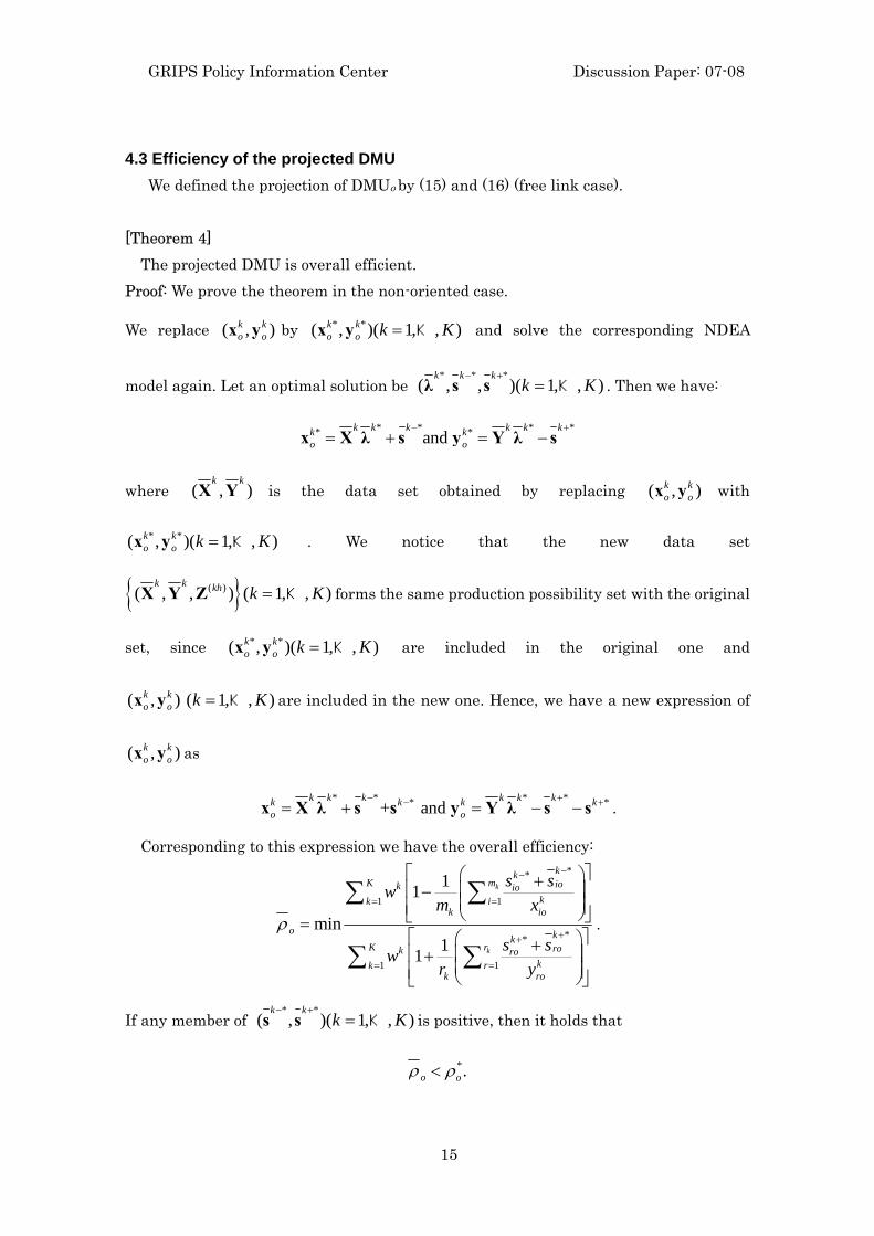
4.3 Efficiency of the projected DMU We defined the projection of DMUo by (15) and (16) (free link case).
[Theorem 4] The projected DMU is overall efficient. Proof: We prove the theorem in the non-oriented case.
We replace ( , )k ko ox y by * *( , )( 1, , )k k
o o k K=x y K and solve the corresponding NDEA
model again. Let an optimal solution be * * *
( , , )( 1, , )k k k
k K− +
=λ s s K . Then we have:
* * * ** *and k k k k k kk k
o o
− += + = −x X λ s y Y λ s
where ( , )k k
X Y is the data set obtained by replacing ( , )k ko ox y with
* *( , )( 1, , )k ko o k K=x y K . We notice that the new data set
{ }( )( , , ) ( 1, , )k k kh k K=X Y Z K forms the same production possibility set with the original
set, since * *( , )( 1, , )k ko o k K=x y K are included in the original one and
( , )k ko ox y ( 1, , )k K= K are included in the new one. Hence, we have a new expression of
( , )k ko ox y as
* * * ** *+ and k k k k k kk k k k
o o
− +− += + = − −x X λ s s y Y λ s s .
Corresponding to this expression we have the overall efficiency: **
1 1
**
1 1
11
min11
k
k
kkK m iok io
kk ik io
o kkK r rok ro
kk rk ro
s swm x
s swr y
ρ
−−
= =
++
= =
⎡ ⎤⎛ ⎞+⎢ ⎥⎜ ⎟−⎜ ⎟⎢ ⎥⎝ ⎠⎣ ⎦=
⎡ ⎤⎛ ⎞+⎢ ⎥⎜ ⎟+⎜ ⎟⎢ ⎥⎝ ⎠⎣ ⎦
∑ ∑
∑ ∑.
If any member of * *
( , )( 1, , )k k
k K− +
=s s K is positive, then it holds that
*.o oρ ρ<

GRIPS Policy Information Center Discussion Paper: 07-08
16
This contradicts the optimality of *.oρ Thus, we have* *
and ( 1, , )k k
k K− += = =s 0 s 0 K .
Hence, the projected DMU is overall efficient. Similarly we can prove the theorem in the oriented models. Q.E.D. 5. Illustrative examples
We present an illustrative example of electric power companies for describing Network DEA and compare the results with traditional approaches. Also we demonstrate an example with the free link case that has no divisionally efficient DMUs.
5.1 Data
As introduced in Section 2 (Figure 4), the vertically integrated electric power companies consist of several divisions such as generation, transmission and distribution. For illustrative purpose, we choose ten vertically integrated power companies in the U.S. in 1994. The inputs, outputs and links are as follows:
Generation (Div 1): Input 1 = Labor input (number of employees)
Transmission (Div 2) : Input 2 = Labor input (number of employees)
Output 2 = Electric power sold to large customers
Distribution (Div 3): Input 3 = Labor input (number of employees)
Output 3 = Electric power sold to small customers
Link (1-2) = Electric power generated (Output from Generation Division and Input to Transmission Division)
Link (2-3) = Electric power sent (Output from Transmission Division and Input to Distribution Division)
Table 1 exhibits data for inputs, outputs and links of the ten DMUs; A to J.
<Table 1: Sample data>

GRIPS Policy Information Center Discussion Paper: 07-08
17
5.2 Results of black box and separation models
First, we solved the aggregated (black box) model explained in Section 1.1, using Inputs 1, 2 and 3, and Outputs 2 and 3 where Links were neglected (see Figure 2). Throughout this section, we utilized the input-oriented SBM (slacks-based measure) under the variable returns-to-scale (VRS) assumption for evaluating efficiency (see [4]). The column “Black box” in Table 2 reports the results.
Next, we solved the separation model explained in Section 1.2. Table 2 reports the results where “Overall score” indicates the weighted average 0.4×Div1+0.2×Div2+0.4×Div3. 0.4, 0.2 and 0.4 are weights to Div 1, Div 2 and Div 3, respectively, which are utilized in the following Network DEA model. This weight selection is just for illustrative purpose. No significant correlation is observed between the two efficiencies; Aggregation and Overall. This is quite natural, since we neglected the internal linking activities in the former.
<Table 2: SBM scores for black box and separation models>
<Figure 9: Comparisons of scores between black box and separation models>
The scores of the black box model tend to be higher than those of the separation model. Actually, these two models cannot be fairly comparable, because the number of inputs is different between the two models. However, this figure clearly explains that the discriminate power of the black box model is inferior to that of the separation model. In addition, it shows that the ranks of the scores of the two models are not always corresponding, e.g. F is scored worse in the black box model, while better in the separation model.
5.3 Results of network DEA
We now return to the Network DEA model taking account the links inside the black box. We minimize the objective function (7) subject to the constraints (3), and (5a) or (5b), i.e. the input-oriented network model under VRS assumption. As weights to
objective function, we employ 1 0.4w = (Division 1), 2 0.2w = (Division 2) and

GRIPS Policy Information Center Discussion Paper: 07-08
18
3 0.4w = (Division 3). This set of weights conforms to the above weights in Table 2. The results of the fixed link case (5a) are displayed in Table 3 while the free link case (5b) is
exhibited in Table 4 where the overall efficiency ( *θ ) together with divisional efficiencies is displayed. The divisional efficiency means the individual term (8) in the objective function. In the “Reference” column, A1 indicates DMU A in the Division 1.
This means 1 0Aλ > in the optimal solution. Since the constraint (5a) is tighter than
(5b), the overall score of the former is larger than that of the latter for every DMU.
<Table 3: NDEA: Fixed link case >
<Table 4: NDEA: Free link case>
Figure 10 compares scores of the separate model and network models (fixed and free link cases). The trend of three models is roughly similar rather than that of the black box model explained in Figure 9. However, we can find gaps among three models, which must be caused by the difference of assumption on the links among divisions. As we mentioned, the separation model does not take account of the links, and therefore, the gap between the separation and network models implies the “linking effects”. The separation model will be insufficient in the case when there actually exist the linking effects inside DMUs.
Concerning two network models, the scores of the fixed link case exceed or equal to those of the free case. The gap of two models explains “suboptimal link effects”. Figure 11 shows the “suboptimal ratio (SOR)” of links measured as projected links in free case divided by actual links (see Table 4). If there exists the gap between two network models in Figure 10, the suboptimal ratio is not equal to unity, and if the ratio is larger than unity, DMU should increase link value, and vice versa.
<Figure 10: Comparisons of scores among separate and two network models>

GRIPS Policy Information Center Discussion Paper: 07-08
19
<Figure 11: Suboptimal ratio of links>
5.4 Example with no divisionally efficient DMUs
We observe 4 DMUs with the same network structure as the previous example. Table 6 exhibits the data. We solved this problem using the input-oriented free link NDEA model under the CRS assumption and obtained the results exhibited in Table 7. We found no efficient DMU in Division 1, while other divisions have an efficient DMUs; N for Division 2 and L for Division 3. This indicates that all DMUs in Division 1 need improvement. Table 8 reports the projection of inputs, outputs and links onto the efficient frontiers by the formulas (15) and (16). Actually, all inputs to Division 1 are reduced proportionally to their scores of Division 1. On the other hand, other divisions and links have benchmarks that remain unchanged in the projection. This occurrence of vacancy of divisionally efficient DMUs in some division is one of characteristics of this model which cannot be expected by traditional DEA models.
<Table 5: Data for four DMUs>
<Table 6: Results of the input-oriented free link CRS model>
<Table 7: Projection onto efficient frontiers>
6. Extensions In this section, we introduce several extensions of the NDEA model.
6.1 Incorporation of link flows in efficiency measurements In the above cases, link flows do not directly concern with the objective function.
They are related with efficiency scores only through link constraints (5a) or (5b). However, if we want to account their excesses (in the input-oriented case) or shortfalls (in the output-oriented case) into the objective function, we can modify the model as follows.1
1 The results of the modified models are identical to the overall score of separation
GRIPS Policy Information Center Discussion Paper: 07-08
20
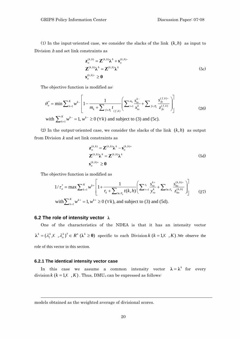
(1) In the input-oriented case, we consider the slacks of the link ( , )k h as input to
Division h and set link constraints as
( , ) ( , ) ( , )
( , ) ( , )
( , )
k h k h h k ho o
k h h k h k
k ho
−
−
= +
=
≥
z Z λ s
Z λ Z λs 0
(5c)
The objective function is modified as:
( , )*
( , )1 1
( , )
1
1min 1
with 1, 0 ( ) and subject to (3) and (5c).
k
k
k
f kkK m fok io
o k f kk i f Pk io fof P f k
K k kk
sswm t x z
w w k
θ−−
−= = ∈
∈
− −=
⎡ ⎤⎛ ⎞⎢ ⎥= − +⎜ ⎟⎜ ⎟⎢ ⎥+ ⎝ ⎠⎣ ⎦
= ≥ ∀
∑ ∑ ∑∑
∑
(26)
(2) In the output-oriented case, we consider the slacks of the link ( , )k h as output
from Division k and set link constraints as
( , ) ( , ) ( , )
( , ) ( , )
( , )
k h k h k k ho o
k h h k h k
k ho
+
+
= −
=
≥
z Z λ s
Z λ Z λs 0
(5d)
The objective function is modified as
( , )*
( , )1 1
1
11/ max 1( , )
with 1, 0 ( ), and subject to (3) and (5d).
k
k
k
k k hK rk ro ho
o k k hk r h Fk ro hoh F
K k kk
s swr t k h y z
w w k
τ+ +
+= = ∈
∈
+ +=
⎡ ⎤⎛ ⎞⎢ ⎥= + +⎜ ⎟+⎢ ⎥⎝ ⎠⎣ ⎦
= ≥ ∀
∑ ∑ ∑∑∑
(27)
6.2 The role of intensity vector λ
One of the characteristics of the NDEA is that it has an intensity vector
1( , , ) ( )k k k T n kn Rλ λ= ∈ ≥λ λ 0K specific to each Division ( 1, , )k k K= K .We observe the
role of this vector in this section.
6.2.1 The identical intensity vector case
In this case we assume a common intensity vector k=λ λ for every division ( 1, , )k k K= K . Thus, DMUo can be expressed as follows:
models obtained as the weighted average of divisional scores.
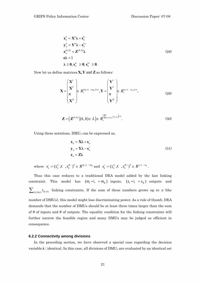
GRIPS Policy Information Center Discussion Paper: 07-08
21
( , ) ( , )
1, , .
k k ko ok k ko ok h k h
o
k ko o
−
+
− +
= +
= −
==
≥ ≥ ≥
x X λ s
y Y λ s
z Z λeλλ 0 s 0 s 0
(28)
Now let us define matrices and X,Y Z as follows:
1 1
1 1
2 2( ) ( ), ,K Km m n r r n
K K
R R+ + × + + ×+ +
⎛ ⎞ ⎛ ⎞⎜ ⎟ ⎜ ⎟⎜ ⎟ ⎜ ⎟= ∈ = ∈⎜ ⎟ ⎜ ⎟⎜ ⎟ ⎜ ⎟⎜ ⎟ ⎜ ⎟⎝ ⎠ ⎝ ⎠
X YX Y
X Y
X Y
L L
M M (29)
( ) ( )( , )( , )( , ) ( , ) .k hk h Lt nk h k h L R ∈
×
+∑= ∈ ∈Z Z (30)
Using these notations, DMUo can be expressed as,
o o
o o
o
−
+
= +
= −=
x Xλ s
y Yλ sz Zλ
(31)
where 11( , , ) Km mK To o os s s R + +− − −= ∈ LK and 11( , , ) Kr rK T
o o os s s R + ++ + += ∈ LK .
Thus this case reduces to a traditional DEA model added by the last linking constraint. This model has 1( )Km m+ +L inputs, 1( )Ks s+ +L outputs and
( , )( , ) k hk h Lt
∈∑ linking constraints. If the sum of these numbers grows up to n (the
number of DMUs), this model might lose discriminating power. As a rule of thumb, DEA demands that the number of DMUs should be at least three times larger than the sum of # of inputs and # of outputs. The equality condition for the linking constraints will further narrow the feasible region and many DMUs may be judged as efficient in consequence.
6.2.2 Connectivity among divisions
In the preceding section, we have observed a special case regarding the decision variable λ ; identical. In this case, all divisions of DMUo are evaluated by an identical set
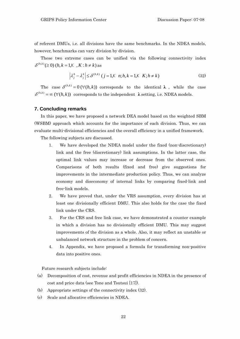
GRIPS Policy Information Center Discussion Paper: 07-08
22
of referent DMUs, i.e. all divisions have the same benchmarks. In the NDEA models, however, benchmarks can vary division by division.
These two extreme cases can be unified via the following connectivity index ( , ) ( 0) ( , 1, , : )h k h k K h kδ ≥ = ≠K as
( , ) ( 1, ; , 1, ; )h k h kj j j n h k K h kλ λ δ− ≤ = = ≠K K (32)
The case ( , ) 0 ( ( , ))h k h kδ = ∀ corresponds to the identical λ , while the case ( , ) ( ( , ))h k h kδ = ∞ ∀ corresponds to the independent λ setting, i.e. NDEA models.
7. Concluding remarks
In this paper, we have proposed a network DEA model based on the weighted SBM (WSBM) approach which accounts for the importance of each division. Thus, we can evaluate multi-divisional efficiencies and the overall efficiency in a unified framework.
The following subjects are discussed. 1. We have developed the NDEA model under the fixed (non-discretionary)
link and the free (discretionary) link assumptions. In the latter case, the optimal link values may increase or decrease from the observed ones. Comparisons of both results (fixed and free) give suggestions for improvements in the intermediate production policy. Thus, we can analyze economy and diseconomy of internal links by comparing fixed-link and free-link models.
2. We have proved that, under the VRS assumption, every division has at least one divisionally efficient DMU. This also holds for the case the fixed link under the CRS.
3. For the CRS and free link case, we have demonstrated a counter example in which a division has no divisionally efficient DMU. This may suggest improvements of the division as a whole. Also, it may reflect an unstable or unbalanced network structure in the problem of concern.
4. In Appendix, we have proposed a formula for transforming non-positive data into positive ones.
Future research subjects include: (a) Decomposition of cost, revenue and profit efficiencies in NDEA in the presence of
cost and price data (see Tone and Tsutsui [17]). (b) Appropriate settings of the connectivity index (32). (c) Scale and allocative efficiencies in NDEA.

GRIPS Policy Information Center Discussion Paper: 07-08
23
(d) Application to dynamic situation that deals with efficiency change over time. (e) Measurements of economies of vertical integration.
Finally, we hope that this study serves as a basis for extending theory and applications of DEA models which have been growing rapidly worldwide.
Appendix A: How to deal with non-positive data in the SBM and NDEA models
In many DEA models, it is a crucial subject how to deal with negative (or zero) data in the evaluation of efficiency. Negative data should have their duly role in measuring efficiency. A large deficit (loss) is worse than a small one. In this appendix, we propose a scheme for resolving this problem. The SBM model has the objective function as described below.
.1
1min
11
11
∑∑
=+
=−
+
−= s
r rors
m
i ioim
ys
xsρ (A1)
This scheme demands positive data. For non-positive data, we propose the following scheme:
Let us suppose 0≤roy . We define ++
rr yy and by
{ }{ }0min
0max
1
1
>=
>=
=+
=
+
rjrj,n,jr
rjrj,n,jr
yyy
yyy
Κ
Κ (A2)
If the output r has no positive elements, then we define 1 == ++
rr yy . We replace the
term ror ys + in the objective function in the following way. (Notice that we never
change the value roy in the constraints.)
(1) If ++>
rr yy , we replace the term with
.)(
ror
rrrr
yy
yyys
−
−+
+++
+ (A3)
(2) If ++=
rr yy , we replace the term with
GRIPS Policy Information Center Discussion Paper: 07-08
24
,)(
)( 2
ror
rr
yyB
ys
−+
+
+ (A4)
where B is a large positive number, e.g. B = 100.
In any case, the denominator is positive and strictly less than +
ry . Furthermore, it is
in inverse proportion to the distance ror yy −+
. Thus, this scheme takes into account the
magnitude of the non-positive output positively. The score obtained is units invariant, i.e., it is independent of the units of measurement used. Table A1 exhibits an example. DMUs D, E, F and G have non-positive outputs. The score (right) reflects their magnitude. In this case, we have
.1,3 == ++yy
Hence, the denominators of (A3) for the DMUs with non-positive output value are as follows:
.3333.0)3(3
21G,4.0)2(3
21F,5.0)1(3
21E,6666.00321D =
−−×
==−−
×==
−−×
==−×
=
The optimal output slacks (against A) are respectively, .6G,5F,4E,3D ====
<Table A1: A sample non-positive data set and results>
Using these values, we obtained the score in Table A1 by using the output-oriented
VRS SBM model. Non-positive input and link data can be dealt with analogously.

GRIPS Policy Information Center Discussion Paper: 07-08
25
Reference [1] Asai S (2007) Private communication. [2] Banker R, Charnes A, Cooper WW (1984) Some models for estimating technical and scale inefficiencies in data envelopment analysis, Management Science, 30, 1078-1092. [3] Charnes A, Cooper WW, Rhodes E (1978) Measuring the efficiency of decision making units. European Journal of Operational Research, 2, 429-444. [4] Cooper WW, Seiford LM, Tone K (2007) Data Envelopment Analysis: A
Comprehensive Text with Models, Applications, References and DEA-Solver Software, Second Edition, Springer.
[5] Färe R (1991) Measuring Farrell efficiency for a firm with intermediate inputs, Academia Economic Papers, 19:2, 329-340.
[6] Färe R, Grosskopf S (1996) Intertemporal Production Frontiers: With Dynamic DEA. Kluwer Academic Publishers, Boston.
[7] Färe R, Grosskopf S (2000) Network DEA, Socio-Economic Planning Sciences 34, 35-49.
[8] Kaihara K, Kinoshita Y, Yoshida S (2007) Private communication. [9] Koopmans T (1951) An analysis of production as an efficient combination of activities.
In Activity analysis of production and allocation. In Koopmans T (Ed.) Cowles commission for research in economics, monograph, 13, John Wiley and Sons, New York.
[10] Lewis HF, Sexton TR (2004) Network DEA: efficiency analysis of organisations with complex internal structure, Computers & Operations Research 31, 1365-1410.
[11] Löthgren M, Tambour M (1999) Productivity and customer satisfaction in Swedish pharmacies: A DEA network model, European Journal of Operational Research, 115, 449-458.
[12] Pastor JT, Ruiz JL, Sirvent I (1999) An enhanced DEA Russell graph efficiency measure, European Journal of Operational Research, 115, 596-607.
[13] Prieto AM, Zofio JL (2007) Network DEA efficiency in input-output models: With an application to OECD countries, European Journal of Operational Research, 178, 292-304.
[14] Seiford LM, Zhu J (1999) Profitability and marketability of the top 55 U.S. commercial banks, Management Science, 45, 9, 1270-1288.
[15] Sexton TR, Lewis HF (2003) Two-stage DEA: An application to major league baseball, Journal of Productivity Analysis, 19, 227-249.
[16] Tone K (2001) A slacks-based measure of efficiency in data envelopment analysis,

GRIPS Policy Information Center Discussion Paper: 07-08
26
European Journal of Operational Research, 130, 498-509. [17] Tone K, Tsutsui M (2007) Decomposition of cost efficiency and its application to
Japanese-US electric utility comparisons, Socio-Economic Planning Sciences, 41, 91-106.
[18] Tsutsui M, Goto M (2007) A multi-division efficiency evaluation of U.S. electric power companies using a weighted slacks-based measure, Socio-Economic Planning Sciences (forthcoming).
GRIPS Policy Information Center Discussion Paper: 07-08
27
Division 1
Division 2
Input 1
Output 1
Division 3
Output 2
Output 3
Link 1→3
Input 3
Link 1→2
Link 2→3
Input 2
Figure 1: Company with three linked divisions
Division 1
Division 2
Input 2
Output 3
Division 3
Output 1 Output 2
Link 1→3
Input 3
Link 1→2
Link 2→3
Input 1
Figure 2: Aggregation

GRIPS Policy Information Center Discussion Paper: 07-08
28
Division 1
Division 2
Input 1
Output 1
Division 3
Output 2
Output 3
Input 3
Input 2
Link 1→3
Link 1→2
Link 2→3
Link 1→2
Link 2→3
Link 1→3
Figure 3: Separation
Distribution
Sales to Large Customers
Generation
Labor Capital
Fuel
Labor
Capital
Labor Capital
Purchased Power Transmission
Generated Power
Transmitted Power
Sales to Small Customers
Figure 4: Vertically integrated electric power companies

GRIPS Policy Information Center Discussion Paper: 07-08
29
Income
Staff
Doctor Nurse
Income
Pharmacy
Hospital Dietetics
Bed
MaterialStaff Patient
Inpatient
Material
Staff
Clinical Laboratory
Staff
Income
Clinical test
Medication
Radiology
Staff
Income
Radiology Exam.
Income
Figure 5: General hospital
Labor
Capital
Services
Program Production
Material
Labor Capital
Material
Transmission
Program Input
Program Sale
Figure 6: Broadcasting companies

GRIPS Policy Information Center Discussion Paper: 07-08
30
Equity
Assets
Profitability
Labor
EPS
Market Value
Marketability
Revenue Profit
Stock Price
Figure 7: Financial holding companies
Inputs
Outputs
Division k
Links p → k
Division q
Links k → q
Division p
Figure 8: Division
GRIPS Policy Information Center Discussion Paper: 07-08
31
0
0.2
0.4
0.6
0.8
1
1.2
A B C D E F G H I J
Black Box Separate
Figure 9: Comparisons of scores between black box and separation models
0
0.2
0.4
0.6
0.8
1
1.2
A B C D E F G H I J
Separate Fixed Free
Figure 10: Comparisons of scores among separate and two network models
GRIPS Policy Information Center Discussion Paper: 07-08
32
0.8
0.9
1
1.1
1.2
1.3
1.4
A B C D E F G H I J
SOR12SOR23
Figure 11: Suboptimal ratio of links

GRIPS Policy Information Center Discussion Paper: 07-08
33
Table 1: Data Div1 Div2 Div3 Link
DMU Input1 Input2 Output2 Input3 Output3 Link12 Link23
A 0.838 0.277 0.879 0.962 0.337 0.894 0.362
B 1.233 0.132 0.538 0.443 0.18 0.678 0.188
C 0.321 0.045 0.911 0.482 0.198 0.836 0.207
D 1.483 0.111 0.57 0.467 0.491 0.869 0.516
E 1.592 0.208 1.086 1.073 0.372 0.693 0.407
F 0.79 0.139 0.722 0.545 0.253 0.966 0.269
G 0.451 0.075 0.509 0.366 0.241 0.647 0.257
H 0.408 0.074 0.619 0.229 0.097 0.756 0.103
I 1.864 0.061 1.023 0.691 0.38 1.191 0.402
J 1.222 0.149 0.769 0.337 0.178 0.792 0.187
Average 1.020 0.127 0.763 0.560 0.273 0.832 0.290
Table 2: SBM score for aggregation and separation
Separation
Divisional score
DMU
Aggregation
(Black box)
Overall
scorea Div1 Div2 Div3
A 1.000 0.659 0.633 0.662 0.684
B 0.531 0.657 0.260 0.763 1.000
C 1.000 0.984 1.000 1.000 0.959
D 1.000 0.719 0.297 1.000 1.000
E 1.000 0.547 0.202 1.000 0.665
F 0.681 0.844 1.000 0.635 0.792
G 1.000 0.855 0.712 1.000 0.926
H 1.000 0.893 0.787 0.890 1.000
I 1.000 0.915 1.000 1.000 0.786
J 1.000 0.640 0.263 0.672 1.000
Average 0.921 0.771 0.615 0.862 0.881
a Overall score indicates 0.4×Div1 + 0.2×Div2 + 0.4×Div3

GRIPS Policy Information Center Discussion Paper: 07-08
34
Table 3: NDEA: Fixed link case
Divisional score Reference Link
DMU
Overall
Score Div1(0.4) Div2(0.2) Div3(0.4) Div1 Div2 Div3 Link12 Link23
A 0.478 0.633 0.339 0.393 C1,F1 C2,D2,E2,I2 D3,H3 0.894 0.362
B 0.739 0.349 1.000 1.000 C1,G1 B2 B3 0.678 0.188
C 0.968 1.000 1.000 0.919 C1 C2 B3,D3,J3 0.836 0.207
D 0.719 0.297 1.000 1.000 C1,F1 D2 D3,H3 0.869 0.516
E 0.456 0.263 1.000 0.377 C1,G1 E2 D3,H3 0.693 0.407
F 0.719 1.000 0.403 0.596 F1 C2,H2,I2 D3,H3 0.966 0.269
G 0.947 1.000 1.000 0.868 G1 G2 D3,H3 0.647 0.257
H 0.969 0.922 1.000 1.000 C1,G1 H2 H3 0.756 0.103
I 0.832 1.000 1.000 0.581 I1 I2 D3,H3 1.191 0.402
J 0.590 0.288 0.377 1.000 C1,G1 C2,G2,H2 J3 0.792 0.187
Average 0.742 0.675 0.812 0.773 0.8322 0.2898
Table 4: NDEA: Free link case
Divisional score Reference Projected Link
DMU
Overall
Score Div1(0.4) Div2(0.2) Div3(0.4) Div1 Div2 Div3 Link12 SOR12* Link23 SOR23*
A 0.385 0.383 0.383 0.389 C1 C2,D2,E2,I2 D3,H3 0.836 0.935 0.355 0.979
B 0.433 0.260 0.341 0.652 C1 C2 D3,H3 0.836 1.233 0.207 1.101
C 0.968 1.000 1.000 0.919 C1 C2 B3,D3,J3 0.836 1.000 0.207 1.000
D 0.719 0.297 1.000 1.000 C1,F1 D2 D3,H3 0.869 1.000 0.516 1.000
E 0.456 0.263 1.000 0.377 C1,G1 E2 D3,H3 0.693 1.000 0.407 1.000
F 0.484 0.406 0.420 0.593 C1 C2,D2,G2 D3,H3 0.836 0.865 0.267 0.991
G 0.778 0.712 0.740 0.863 C1 C2,D2,G2 D3,H3 0.836 1.292 0.254 0.988
H 0.969 0.922 1.000 1.000 C1,G1 H2 H3 0.756 1.000 0.103 1.000
I 0.832 1.000 1.000 0.581 I(1) I2 D3,H3 1.191 1.000 0.402 1.000
J 0.506 0.271 0.338 0.825 C1,G1 C2,H2 D3,H3 0.821 1.037 0.188 1.005
Average 0.653 0.551 0.722 0.720 0.851 1.036 0.291 1.006
* SOR12 and SOR23 indicate the ratio of the projected link value vs. observed value.

GRIPS Policy Information Center Discussion Paper: 07-08
35
Table 5: Data for four DMUs
Div1 Div2 Div3 Link
DMU Input1 Input2 Output2 Input3 Output3 Link12 Link23
K 3 10 2 5 2 8 2
L 14 1 1 5 5 9 5
M 16 2 2 11 4 7 4
N 19 0.5 2 7 4 11 4
Table 6: Results of the input-oriented free link CRS model
DMU Overall Score Div1(0.4) Div2(0.2) Div3(0.4)
K 0.71 0.875 0.2 0.8
L 0.672 0.368 0.625 1
M 0.299 0.258 0.25 0.364
N 0.515 0.217 1 0.571
Table 7: Projection onto efficient frontiers
Div1 Div2 Div3 Link
DMU Input1 Prj* Input2 Prj Output2 Prj Input3 Prj Output3 Prj Link12 Prj Link23 Prj
K 3 2.625 10 2 2 2 5 4 2 4 8 7 2 4
L 14 5.156 1 0.63 1 2.5 5 5 5 5 9 13.8 5 5
M 16 4.125 2 0.5 2 2 11 4 4 4 7 11 4 4
N 19 4.125 0.5 0.5 2 2 7 4 4 4 11 11 4 4
* Prj indicates projection onto efficient frontiers.

GRIPS Policy Information Center Discussion Paper: 07-08
36
Table A1: A sample non-positive data set and results
DMU (I)x (O)y DMU Score Rank Reference set (λ)
A 1 3 A 1 1 A 1
B 1 2 B 0.667 2 A 1
C 1 1 C 0.333 3 A 1
D 1 0 D 0.182 4 A 1
E 1 -1 E 0.111 5 A 1
F 1 -2 F 0.074 6 A 1
G 1 -3 G 0.052 7 A 1