Newcastle University ePrints

Powell JP, González-Gil A, Palacin R. Experimental assessment of the energy

consumption of urban rail vehicles during stabling hours: influence of

ambient temperature. Applied Thermal Engineering 2014, 66(1-2), 541-547.

Copyright:

©2014 Elsevier Ltd.

NOTICE: this is the author’s version of a work that was accepted for publication in Applied Thermal

Engineering. Changes resulting from the publishing process, such as peer review, editing, corrections,

structural formatting, and other quality control mechanisms may not be reflected in this document.

Changes may have been made to this work since it was submitted for publication. A definitive version

was subsequently published in Applied Thermal Engineering, Vol. 66, Issues 1-2, 2014, DOI:

http://dx.doi.org/10.1016/j.applthermaleng.2014.02.057

Always use the definitive version when citing.

Further information on publisher website: www.elsevier.com

Date deposited: 14-10-2014

Version of file: Accepted Author Manuscript

This work is licensed under a Creative Commons Attribution-NonCommercial 3.0 Unported License

ePrints – Newcastle University ePrints

http://eprint.ncl.ac.uk

Experimental assessment of the energy consumption of urban rail vehicles during

stabling hours: influence of ambient temperature

J.P. Powell a, A. González-Gil a *, R. Palacin a

a NewRail – Centre for Railway Research, Newcastle University, School of Mechanical and Systems

Engineering, Stephenson Building, Newcastle upon Tyne NE1 7RU, UK

* Corresponding author: Arturo González-Gil

email: arturo.gonzalez@newcastle.ac.uk; phone: +44 191 222 8657

Abstract

Urban rail has widely recognised potential to reduce congestion and air pollution in

metropolitan areas, given its high capacity and environmental performance. Nevertheless, growing

capacity demands and rising energy costs may call for significant energy efficiency improvements in

such systems. Energy consumed by stabled rolling stock has been traditionally overlooked in the

scientific literature in favour of analysing traction loads, which generally account for the largest

share of this consumption. Thus, this paper presents the methodology and results of an experimental

investigation that aimed to assess the energy use of stabled vehicles in the Tyne and Wear Metro

system (UK). It is revealed that approximately 11% of the rolling stock’s total energy consumption is

due to the operation of on-board auxiliaries when stabled, and investigation of these loads is

therefore a worthwhile exercise. Heating is responsible for the greatest portion of this energy, and

an empirical correlation between ambient temperature and power drawn is given. This could prove

useful for a preliminary evaluation of further energy saving measures in this area. Even though this

investigation focused on a particular metro system in a relatively cold region, its methodology may

also be valid for other urban and main line railways operating in different climate conditions.

Keywords: urban rail; experimental investigation; energy consumption; on-board auxiliary systems,

temperature dependence.

1. Introduction

Metropolitan transportation is responsible for about 25% of the CO2 emissions caused by the

transport sector in the European Union (EU) (European Commission, 2011), which approximately

represents 8% of total greenhouse gas emissions in the EU (IEA & UIC, 2012). Furthermore, high

levels of air pollution and congestion are major problems usually associated with urban mobility.

Therefore, more efficient, reliable and environmentally friendly transport systems are key in dealing

with increasing urbanisation, whilst reducing GHG emissions and enhancing living conditions in

urban areas.

Urban rail is well placed to mitigate the impact of the problems associated with urban mobility

because of its high capacity, safety, reliability and absence of local emissions (Vuchic, 2007). In

addition, it typically has lower CO2 emissions per passenger than competing transportation modes,

although this is dependent on passenger load factors and the electricity generation mix (Chester &

Horvath, 2009). Nevertheless, in a context characterised by rising energy costs and growing capacity

demands, and where other modes such as automotive are making significant improvements in their

environmental performance, it is critical that urban rail minimises its energy consumption while

enhancing its service quality.

Energy use in railway systems is commonly classified into traction and non-traction loads. The

former comprises the power required to operate the rolling stock across the system (including

propulsion and on-board auxiliary systems), whereas the latter accounts for the energy utilised at

stations, depots and other facilities in the system. On average, traction energy consumption

generally represents between 70% and 90% of the total energy consumption in urban rail systems,

of which around 20% is due to on-board auxiliaries (González-Gil, et al., currently under review).

Hence, the majority of proposals to reduce energy consumption in railway systems have focused on

the traction system itself, primarily by using regenerative braking (González-Gil, et al., 2013),

applying energy-efficient driving strategies (De Martinis, et al., 2013), or improving the propulsion

chain efficiency (Kondo, 2010). In turn, there has been relatively less focus on the on-board auxiliary

systems.

Auxiliary power is required for two main purposes: control and cooling of vehicle systems, and

comfort functions – these include heating, ventilation and air-conditioning (HVAC), lighting and

information systems. HVAC equipment is generally responsible for the most significant part of this

consumption, with a clear dependency on climate conditions. In the Oslo metro for instance, heating

accounts for 78% of the auxiliary consumption, with 3% for control systems and the remaining 19%

for other auxiliaries such as lighting and air supply (Struckl, et al., 2006). This corresponds to

heating accounting for 28% of the vehicle consumption overall. In addition, variations of up to 38%

in the total energy consumption were found between summer and winter months for a fleet of

regional trains operating in Sweden (Andersson & Lukaszewicz, 2006).

On-board auxiliary systems remain partially or fully operative while trains are stabled in sidings or

depots. This is principally to facilitate cleaning operations and to prevent damage to vulnerable

components, for example any condensation in the air supply system freezing overnight. Furthermore,

it is necessary to reach the desired comfort conditions (such as temperature) in vehicles before they

enter service. Therefore, the operation of on-board auxiliaries while trains are out of service may

account for a significant portion of the total energy consumption – for example general studies of

Central and Northern Europe main line services estimated energy consumption of stabled trains to

be around 10–15% of the system’s total energy consumption (UIC, 2003), (Peckham, 2007). The

scarcity of information and experimental data published in the academic literature – particularly for

the case of urban rail – seems to call for more thorough investigations.

The main purpose of this paper is therefore to develop a deeper understanding and promote

awareness of power consumed by rail vehicles while stabled. To achieve this, the outcomes of an

experimental investigation aimed at assessing the energy use of stabled vehicles in the Tyne and

Wear Metro (UK) are presented. The paper starts by briefly describing the Metro system, continues

by explaining the research methodology and concludes by showing and discussing the main energy

consumption results obtained for a single vehicle while stabled. Special emphasis is placed on

examining the influence of ambient temperature upon the on-board auxiliaries’ energy consumption.

Although this paper focuses on an urban rail system as the specific case study, it is intended that the

methodology described could be applied to all rail systems.

2. Introduction to the Tyne and Wear Metro system

2.1. General description and climate conditions

The Tyne and Wear (T&W) Metro is a light rail system centred on Newcastle upon Tyne in the north-

east of England. First opened in 1980 as a 54 km route (of which 41 km had been adapted from

existing heavy-rail tracks), currently the T&W Metro consists of a 78 km network that links the cities

of Sunderland, Gateshead and Newcastle with the local airport and coastal regions. It is the second

largest urban rail system in the UK (after London Underground), and the only one powered by an

overhead 1500 V DC supply network. Further details on the T&W Metro can be found in (Howard,

1976), (Prickett, 1981), (Mackay, 1999) and (Pflitsch, et al., 2012).

The original rolling stock remains in service today, although it was refurbished between 1995 and

2000, and is currently undergoing life extension work to run until the mid-2020s. The fleet consists

of ninety identical 28 m long twin-section articulated Metrocars built by Metro-Cammell; there are

68 seats, although around 300 passengers may be carried under crush load conditions. A single

articulated Metrocar is carried on three two-axle bogies, with each outer bogie powered by a 185 kW

series-wound DC monomotor, resistance-controlled by an air/oil camshaft. Braking is a combination

of rheostatic and spring applied/air released friction brakes. The typical train configuration consists

of two Metrocars, although single unit operation is also possible.

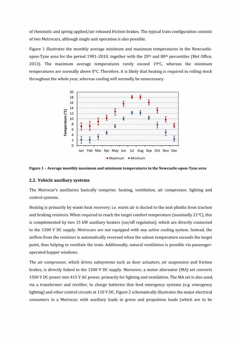
Figure 1 illustrates the monthly average minimum and maximum temperatures in the Newcastle-

upon-Tyne area for the period 1981–2010, together with the 20th and 80th percentiles (Met Office,

2013). The maximum average temperatures rarely exceed 19°C, whereas the minimum

temperatures are normally above 0°C. Therefore, it is likely that heating is required in rolling stock

throughout the whole year, whereas cooling will normally be unnecessary.

Figure 1 – Average monthly maximum and minimum temperatures in the Newcastle-upon-Tyne area

2.2. Vehicle auxiliary systems

The Metrocar’s auxiliaries basically comprise: heating, ventilation, air compressor, lighting and

control systems.

Heating is primarily by waste heat recovery; i.e. warm air is ducted to the seat plinths from traction

and braking resistors. When required to reach the target comfort temperature (nominally 21°C), this

is complemented by two 15 kW auxiliary heaters (on/off regulation), which are directly connected

to the 1500 V DC supply. Metrocars are not equipped with any active cooling system. Instead, the

airflow from the resistors is automatically reversed when the saloon temperature exceeds the target

point, thus helping to ventilate the train. Additionally, natural ventilation is possible via passenger-

operated hopper windows.

The air compressor, which drives subsystems such as door actuators, air suspension and friction

brakes, is directly linked to the 1500 V DC supply. Moreover, a motor alternator (MA) set converts

1500 V DC power into 415 V AC power, primarily for lighting and ventilation. The MA set is also used,

via a transformer and rectifier, to charge batteries that feed emergency systems (e.g. emergency

lighting) and other control circuits at 110 V DC. Figure 2 schematically illustrates the major electrical

consumers in a Metrocar, with auxiliary loads in green and propulsion loads (which are to be

0

2

4

6

8

10

12

14

16

18

20

Jan Feb Mar Apr May Jun Jul Aug Sep Oct Nov Dec

Te

mp

era

ture

(°C

)

Maximum Minimum

excluded from this study) in red. Note that in reality the equipment is distributed between both

sections of the Metrocar.

Figure 2 – Simplified illustration of Metrocar electrical circuits

2.3. Stabling

The T&W Metro has one depot located in Gosforth. Amongst other facilities, the site comprises: the

running shed, where Metrocars are stabled between service duties; the inspection shop, where

routine maintenance and light repairs are performed; and the lifting shop, where heavy duty repairs

are carried out. Whereas the running shed is unsealed and unheated, both the inspection and lifting

shops include a heating system that aims to keep the indoor air temperature around 15°C. Due to the

fleet size, some vehicles have to be stabled outdoors, others will be in the inspection shop overnight

for stabling and maintenance, and vehicles are also moved during the night as required.

In principle, all of the Metrocar’s auxiliary systems remain in operation when stabled, unless isolated

from the overhead power supply for certain maintenance tasks. Among others, this means that the

heating remains on to maintain the target interior temperature, which in this case is the same as in-

service.

3. Methodology

3.1. Data collection

Data collected between 1st April 2012 and 31st March 2013 from an energy meter fitted to Metrocar

number 4067 forms the basis for the analysis in this paper. Further instrumentation of the vehicle,

such as vehicle subsystem metering or air temperature sensors, was not possible within the scope of

the experimental programme. The following parameters were recorded every second: overhead line

voltage, current and power drawn from the overhead line, output voltage from the MA set (for both

the 425 V and 110 V circuits) and train speed. Field data were remotely downloaded in .csv format to

computers in the depot offices, before being processed using Matlab and Microsoft Excel.

Camshaft resistance Compressor Saloon heaters MA set

Braking resistorsTraction motor

VentilationControl circuits

Propulsion loads Auxiliary loads

1500V DC

415V AC110V DC

Lighting

Historical climate data for the trial period were obtained from the weather station at Newcastle

International Airport, which is located around 6 km from the depot in Gosforth (Weather

Underground, 2013). This principally comprises ambient temperature, degree of cloudiness and

wind speed. Global solar irradiance values were estimated by using the “very simple cloudy sky

model” suggested by (Badescu, 1997). Solar position throughout the year was obtained using the

algorithm proposed by (Reda & Andreas, 2004).

3.2. Data reduction

Although data is sampled by the energy meter every second, the basic time step selected to reduce

experimental measurements for further analysis was of 30 minutes, since this is the sampling

frequency of the available weather data. Note that this selection is also of the same order of

magnitude as the typical thermal time constant of rail vehicles, reported to be around one hour by

(Tomlinson, 1988). Thus, the distance travelled each second was summed within each 30 minute

time step, and likewise the second-by-second power consumption was used to provide average

power consumption data. If there was no movement within the 30 minutes, it was assumed that the

Metrocar was stabled, as this time period is in excess of the typical turnaround times at terminal

stations (5-15 minutes).

3.3. Data analysis

The data analysis methodology can be summarised as follows:

1. Calculating the total energy consumption of the unit for the whole experimental

period, including running and stabling hours.

2. Determining the number of hours the vehicle was stabled, and the corresponding

energy consumption for this period.

3. Investigating the relationship between ambient temperature and the vehicle’s energy

consumption while stabled.

4. Examining factors that may influence the above relationship.

5. Analysing further experimental results to determine the breakdown of energy

consumption between systems (including heating, lighting, air compressor and

others).

4. Experimental results and discussion

This investigation involved collecting data during real operation of the metro system; hence, there

were some unavoidable discontinuities in the measurements, mostly corresponding to the time

where the unit was undergoing maintenance and the pantograph had been dropped. Some data were

also corrupted in process of transmission to the depot. In total, there were 28 days out of 365 that

could not be used for the purpose of this study.

4.1. Vehicle’s total energy consumption

The total energy consumption of Metrocar 4067 during the 337 days of the trial period was 515,696

kWh, for a total travelled distance of around 130,000 km. Figure 3 illustrates the full data set for this

period, with each point representing the distance travelled and energy consumed on a particular

day, and the colour showing the average temperature of that day. As expected, the total energy

consumption is proportional to distance travelled, with an additional offset on the y-axis that

principally accounts for the auxiliaries’ energy consumption, although other factors such as the

driving style or traffic conditions may also have some influence. The general trend observed in the

spread indicates that energy consumption is noticeably higher on colder days, which suggests that

heating accounts for a substantial proportion of the auxiliaries’ energy consumption. In fact, about

95% of the values lie within the range of 725 kWh per day, which on average corresponds to the

auxiliary heaters’ power of 30 kW.

Figure 3 – Daily energy consumption of Metrocar 4067 during the trial period 2012–2013

4.2. Vehicle’s energy consumption while stabled

4.2.1. Overall energy consumption and distribution of stabled time

Experimental data show that unit 4067 was stabled for 3,895 hours during the 337days of the trial

period, which represents about 48% of the total time. Figure 4 depicts the average daily distribution

of time stabled for this unit; or in other words, it shows the probability of finding this Metrocar

stabled at the depot at any time of the day during the trial period. The trend shown in this figure is

representative of the timetable of T&W Metro, where peak time services are operational in both

directions from approximately 7:00 to 10:00, and from 16:00 to 18:00. Note that vehicles may be

moved around the depot at night, which accounts for the small percentage of time not stabled

overnight.

0

500

1000

1500

2000

2500

3000

3500

0 100 200 300 400 500 600 700

En

erg

y c

on

sum

ed

(k

Wh

)

Daily distance travelled (km)

725

kWh

- 4ºC

19ºC

Ave

rag

e d

ail

y t

em

pe

ratu

re

Figure 4 – Daily distribution of stabled time for Metrocar 4067 during the trial period 2012–2013

The energy consumed by unit 4067 while stabled was of 56,059 kWh for the whole trial period; i.e.

an average of 166 kWh per day. This means that about 11% of the vehicle’s total energy

consumption occurred while stabled.

4.2.2. Influence of ambient temperature

In order to assess the contribution of each auxiliary system, energy consumption on those days

where the Metrocar was stabled for the whole day were examined (these days correspond to the

points on the y-axis in Figure 3). In this manner, the effects of remaining heat from brake resistors

and other influencing factors associated with train operations were minimised.

Figure 5 compares the half-hourly averages of the Metrocar’s power consumption and the ambient

temperature for a day where it was always stabled (12th May 2012). A clear correlation between

these variables may be observed, with higher power consumption at lower temperatures.

Figure 5 – Average power consumption of Metrocar 4067 on 12th May 2012

Figure 6 illustrates the power consumption results for a different day of the experimental campaign

(15th April 2012). It can be observed that the power consumption initially varied with the ambient

temperature, similarly to that found for the previous example. However, after a period during which

the unit was registered to move a few hundred metres, the power consumption remained nearly

constant around 8 kW. This suggests that the heating was not needed any longer after the vehicle

was shifted into an enclosed and heated building (refer to section 2.3). Note that the average power

consumption for the period in which the vehicle moved was not plotted in Figure 6, as traction and

auxiliary energy consumption cannot be separated in the measurements.

Figure 6 – Comparison of power-temperature relationship outside and inside depot shed (unit 4067,

15th April 2012)

In order to determine the relationship between ambient temperature and vehicle energy

consumption while stabled, the results from 14 different days where it could be established with

reasonable confidence that the Metrocar was stabled outdoors were combined; the pairs of

temperature and power consumption for each half hour period are illustrated in Figure 7.

Figure 7 – Relationship between ambient temperature and power consumption for unit 4067 and

influence of solar gains

At the highest and lowest temperatures, the power consumption is roughly independent of

temperature, whereas an approximately linear relationship is observed in the central region of

Figure 7 . The empirical correlation that provided the best fit to these results is described by

Equation (1), where P is the power consumption (in W) and Ta is the ambient temperature (in °C).

� = �38000� < 0−2500� + 380000 ≤ � ≤ 128000� > 12 � (1)

The starting point for constructing a best fit line was to find the average power consumption in the

tightly clustered region above 15°C where the heating is always off. The power consumption in the

coldest region will then be about 30 kW above this value, as this is the rating of the auxiliary heaters.

To obtain the relationship in the central region, a set of linear best fit lines to the data using different

temperature pairs for the transitions to the region where heating is on intermittently were plotted,

and it was found that using boundaries of 0°C and 12°C gave the best correlation to the data in this

region, with an R2 value of 0.8.

The global solar irradiance is also displayed on the graph (Figure 7); there appears to be an

additional weak relationship whereby higher solar irradiance reduces the power consumption,

independent of the ambient temperature. This, and other second order factors, are examined in

more detail in section 4.2.3 below.

4.2.3. Discussion of the relationship between temperature and power consumption

It is proposed that the auxiliary power consumption illustrated in Figure 7 can be divided into two

components: the heating, which is dependent on temperature, and other systems, which should have

0

5

10

15

20

25

30

35

40

45

-5 -3 -1 1 3 5 7 9 11 13 15 17 19 21

Po

we

r co

nsu

mp

tio

n (

kW

)

Temperature (°C)

Actual data

Trend line

I = 0

0 < I ≤ 300

300 < I ≤ 500

I > 500

Global solar irradiance on

horizontal plane (W/m2)

an approximately constant power consumption when examined over half hour periods. There will

also be second order effects (such as global solar irradiance mentioned above) that may increase the

scatter in the results beyond what would be expected from experimental inaccuracies and errors

alone. This section therefore examines three regions of Figure 7 defined by the temperatures, and

the scatter.

High temperature region

At higher temperatures, the heaters should be off and the power consumption therefore constant;

this is observed to happen at temperatures above 12–13°C in Figure 7, where the power

consumption is around 8 kW in Figure 7. This figure is consistent with the power consumption in

Figure 6 for when the Metrocar is assumed to be stabled within a heated building. To validate these

findings, further data analysis and an independent set of experiments was carried out at the depot

(this new experimental data was gathered from Unit 4088). Different auxiliary systems were

switched on/off independently, and the variation in power drawn from the overhead line recorded,

to compare against derived values:

� Compressor – second-by-second data from 12th August 2012 was inspected, and

revealed power peaks of about 15 kW, lasting for around 12 seconds, at intervals of

around 5 minutes, which represents a mean power draw of 0.6 kW. The experiment

confirmed that these power peaks matched those observed when the compressor was

running.

� Lighting – the main saloon lighting is provided by 38 fluorescent bulbs of 40 W each,

and the measured power draw of 1.5 kW matches this.

� Other MA set circuits – the remaining circuits, which include ventilation fans, battery

charger and control equipment, drew a mean power of 6 kW in the experiment.

Together, these figures provide excellent agreement with the previously derived overall value of a

constant 8 kW of power for these auxiliary systems.

Low temperature region

At low temperatures, the heaters are permanently on and therefore consuming their maximum rated

power of 30 kW (refer to section 2.2). This corresponds to temperatures below 0 °C in Equation (1)

where the power consumption is no longer dependent on temperature.

Intermediate temperature region

At intermediate temperatures in the central region of Figure 7, an approximately linear relationship

between temperature and power consumption may be observed. This is consistent with the general

equation governing the steady heat demand in stabled rail vehicles without occupation and without

solar load, simplified as follows (Ampofo, et al., 2004):

���� = ����� + ����� −������ = ∑ ! ∙ #�� − �$ + %& �' ∙ (),�' ∙ #�� − �$ − ������ (2)

where Qcond represents the heat losses through the vehicle’s envelope, essentially due to conductive

heat transfer; Qvent is the heat load due to ventilation and air infiltration; Qlight represents the heat

emitted by equipment within the vehicle such lighting; U and A are the global heat transfer and the

area of each surface forming the vehicle’s envelope respectively; %& �' is the mass flow rate of air

supply into the vehicle; cp,air is the ambient air specific heat; Ti and Ta are the indoor and ambient air

temperatures respectively.

All variables in the right hand side of Equation (2) – except for Ta – should be practically constant

when the vehicle is stabled at the depot, which means that the heating power consumption should be

approximately linearly dependent on the ambient temperature. This would explain the linear trend

found in the experimental data; however, there is a series of second order factors that equation (2)

does not consider and that may affect the vehicle’s thermal load.

The precise location of the transition points between the intermediate temperature region and

low/high temperature regions was determined by finding the transition temperatures that provided

the best fit to the data in the central region.

Scatter

Figure 7 nonetheless shows a significant spread in the experimental data from the proposed trend

line, including a variation of up to about 15 kW in energy consumption for the same temperature on

different days. This may be due to unpredictable causes such as fluctuations in the air temperature

adjacent to the temperature sensor, the influence of adjacent buildings/vehicles, equipment

reliability, or changeable boundary conditions (e.g. windows may be left open during night-time).

The effect of body thermal storage could also be suggested as a possible reason, although this effect

has been identified to be very limited in the case of rail vehicles (Liu, et al., 2011), (Amri, et al.,

2011). The influence of ambient air speed and incident solar radiation may play a more significant

role yet (Ampofo, et al., 2004), (Li & Sun, 2013).

Higher ambient air velocities tend to increase the heat transfer through the vehicle’s envelope, since

this improves heat transfer coefficient U. However, this effect has been found to be rather limited in

this particular case: preliminary calculations showed that wind speeds of 35 m/s (the highest value

observed during the trial period) will only cause an increase of about 5% in the Metrocar’s thermal

load, in comparison with still conditions.

In turn, the influence of solar radiation appears to be stronger, as can be deduced from Figure 7. It is

observed that most of the points below the trend line correspond to medium/high values of global

solar irradiance (over 300 W/m2 on a horizontal plane). Conversely, the majority of the points above

the line correspond to little or no solar radiation. Furthermore, calculations made according to BS

EN 14750-2 (2006) (BSI, 2006) have revealed that solar irradiance values of around 800 W/m2 (the

highest value observed during the trial period) may imply heat gains of up to 10 kW in vehicles

stabled outdoors. Therefore, it may be concluded that the variable incident solar radiation is a major

reason for the scatter observed in Figure 7; this being particularly valid for ambient temperatures

between 3°C and 12°C, where the range of solar irradiance values is wider.

4.2.4. Summary of the breakdown of energy consumption

As concluded above, auxiliaries’ power consumption excluding heating may be considered fairly

constant throughout the year, with an average value of 8 kW. Hence, considering the Metrocar was

stabled for about 3,895 hours during the trial period (section 4.2.1), the energy consumption due to

those systems can be estimated as 31,160 kWh. This means that heating was responsible for about

24,899 kWh, which represents nearly 45% of the vehicles’ total consumption while stabled.

HVAC systems therefore play a key role in the auxiliary energy consumption of stabled Metrocars,

with the ambient temperature being the main influencing factor in such consumption. Solar

radiation – and to a less extent wind speed – may also have an influence depending on the location of

the vehicle; that is, depending whether there are other vehicles or buildings adjacent providing

shade or disrupting the wind. Moreover, there is a combination of other essentially unpredictable

factors such as uncontrolled ambient air infiltration (e.g. through open windows) and fluctuations in

local air temperature that can also have a significant effect on the consumption.

Figure 8 gives a graphical summary of the approximate energy consumption breakdown of stabled

Metrocars, based on the results of section 4.2.3. Note that the energy consumptions depicted herein

do not separate inefficiencies and energy losses within subsystems, which could not be evaluated in

the present investigation.

In service

89%

Ventilation,

Control & Others

41%

Heating

45%Compressor

4%

Lighting

10%

Stabled

11%

Figure 8 – Breakdown of main auxiliaries’ energy consumption in stabled Metrocars

4.3. Uncertainty analysis

Table 1 shows the experimental uncertainties of the main variables used in this investigation. The

values for both the power consumption and the distance travelled are directly drawn from the

energy meter specifications, whereas the ambient temperature uncertainty is given by the weather

data providers (Weather Underground, 2013).

Table 1 – Experimental uncertainties

Variable Uncertainty

Power consumption 2%

Distance travelled 4%

Ambient temperature ±1°C

The uncertainties in Table 1 can account for some of the scatter in Figure 7, and the effects are not

negligible when compared to the factors mentioned in section 4.2.3. Nonetheless, given the volume

of data analysed, and the strength of the correlation between ambient temperature and power

consumption, it is considered that the results presented in this paper are reasonably robust.

5. Conclusions

In order to investigate the energy use of stabled rolling stock in urban rail systems, power

consumption and distance travelled by one of the 90 Metrocars forming the T&W Metro fleet were

measured for one year. The following conclusions have been drawn from the analysis of the

experimental data obtained:

It has been found that approximately 11% of the Metrocar’s yearly energy consumption is accounted

for by on-board auxiliary systems while the vehicle is stabled. Heating has been shown to be

responsible for about 45% of this consumption, while the lighting and compressed air systems

account for 10% and 4% respectively; other consumptions including fans and control circuits

represent 41% of the total stabled energy consumption.

Ambient temperature has been identified as the main influencing factor on stabled vehicles’ energy

consumption, although solar radiation and wind speed may also have a notable influence depending

upon the vehicle’s location at depots.

A correlation between ambient temperature and the stabled vehicle’s energy consumption has been

obtained empirically. Although further experiments would be needed to develop a more accurate

model, this correlation may be used as a preliminary tool in the evaluation of possible measures to

minimise the energy consumed by stabled Metrocars. The results obtained for a single unit could be

extrapolated to fleet level, as all the vehicles are of the same type/age and present similar duty

cycles.

Ultimately, this paper has shown that the energy consumed by stabled vehicles is not negligible in

comparison with energy consumed in service, and investigation of measures to reduce this

consumption is a worthwhile exercise. Although the characteristics (and hence the specific results

for the breakdown of energy use and the dependence on ambient temperature) will be different for

other urban and main line railway systems, this conclusion is likely to remain valid, and the

methodology outlined in this paper can be applied to other systems.

Acknowledgements

The authors would like to thank DB Tyne & Wear Ltd., the operator of Tyne & Wear Metro, for the

opportunity to carry out this research and the access to the relevant data.

References

Ampofo, F., Maidment, G. & Missenden, J., 2004. Underground railway environment in the UK

Part 2: Investigation of heat load. Appl Therm Eng, 24(5-6), pp. 633-645.

Amri, H., Hofstädter, R. N. & Kozek, M., 2011. Energy efficient design and simulation of a

demand controlled heating and ventilation unit in a metro vehicle. Vienna (Austria), IEEE Forum on

Integrated and Sustainable Transportation Systems, FISTS 2011.

Andersson, E. & Lukaszewicz, P., 2006. Energy consumption and related air pollution for

Scandinavian electric passenger trains, Stockholm, Sweden: Royal Institute of Technology (KTH).

Badescu, V., 1997. Verification of some very simple clear and cloudy sky models to evaluate

global solar irradiance. Solar Energy, 61(4), p. 251–264.

BSI, 2006. BS EN 14750-2:2006 – Railway applications – Air conditioning for urban and

suburban rolling stock – Part 2: Type tests. London: British Standards.

Chester, M. V. & Horvath, A., 2009. Environmental assessment of passenger transportation

should include infrastructure and supply chains. Environmental Research Letters, 4(2), p. 1–8.

De Martinis, V., Gallo, M. & D'Acierno, L., 2013. Estimating the benefits of energy-efficient train

driving strategies: A model calibration with real data. WIT Transactions on the Built Environment ,

Volume 130, p. 201–211.

European Commission, 2011. Roadmap to a Single European Transport Area – Towards a

competitive and resource efficient transport system, s.l.: http://eur-

lex.europa.eu/LexUriServ/LexUriServ.do?uri=COM:2011:0144:FIN:en:PDF.

González-Gil, A., Palacin, R. & Batty, P., 2013. Sustainable urban rail systems: Strategies and

technologies for optimal management of regenerative braking energy. Energy Conversion and

Management, Volume 75, p. 374–388.

González-Gil, A., Palacin, R., Batty, P. & Powell, J. P., currently under review. A systems

approach to reduce urban rail energy consumption. Energy Conversion and Management.

Howard, D. F., 1976. Tyne and Wear Metro – A modern rapid transit system. Proceedings of the

Institution of Mechanical Engineers, Volume 190, p. 121–136.

IEA & UIC, 2012. Railway handbook 2012 - Energy consumption and CO2 emissions.

s.l.:http://www.uic.org/IMG/pdf/iea-

uic_energy_consumption_and_co2_emission_of_world_railway_sector.pdf.

Kondo, K., 2010. Recent energy saving technologies on railway traction systems. IEEJ

Transactions on Electrical and Electronic Engineering, Volume 5, pp. 298-303.

Liu, W., Deng, Q., Huang, W. & Liu R, 2011. Variation in cooling load of a moving air-

conditioned train compartment under the effects of ambient conditions and body thermal storage.

Applied Thermal Engineering, Volume 31, pp. 1150-1162.

Li, W. & Sun, J., 2013. Numerical simulation and analysis of transport air conditioning system

integrated with passenger compartment. Applied Thermal Engineering, 50(1), pp. 37-45.

Mackay, K. R., 1999. Sunderland Metro - Challenge and Opportunity. Proceedings of the

Institution of Civil Engineers: Municipal Engineer, 133(2), p. 53–63.

Met Office, 2013. UK Climate averages. [Online]

Available at: http://www.metoffice.gov.uk/climate

[Accessed November 2013].

Peckham, C., 2007. Improving the efficiency of traction energy use,

http://www.rssb.co.uk/SiteCollectionDocuments/pdf/reports/research/T618_traction-rpt_final.pdf:

Rail Safety and Standards Board.

Pflitsch, A. et al., 2012. Air flow measurements in the underground section of a UK light rail

system. Applied Thermal Engineering, 32(1), pp. 22-30.

Prickett, B. R., 1981. Electrification of the Tyne and Wear Metro. Electric Power Applications,

IEE Proceedings B, 128(2), p. 81–91.

Reda, I. & Andreas, A., 2004. Solar position algorithm for solar radiation applications. Solar

Energy, Volume 76, p. 577–589.

Struckl, W., Stribersky, A. & Gunselmann, W., 2006. Life cycle analysis of the energy

consumption of a rail vehicle. Berlin, Germany, International Workshop of Allianz pro Schiene:

Improvement of the environmental impacts of rail transport – challenges, good practices and future

challenges.

Tomlinson, B. A., 1988. A study of southern region's electric traction energy costs, s.l.: British

Rail Research TM ES 086.

UIC, 2003. Energy Efficiency Technologies for Railways. [Online]

Available at: http://www.railway-energy.org

[Accessed September 2013].

Vuchic, V. R., 2007. Urban transit systems and technology. Hoboken, New Jersey: John Wiley &

Sons, Inc..

Weather Underground, 2013. Weather History for Newcastle Airport, United Kingdom. [Online]

Available at:

http://www.wunderground.com/history/airport/EGNT/2014/1/31/DailyHistory.html?MR=1

[Accessed November 2013].