Newcastle University ePrints

Marinov M, Sahin I, Ricci S, Vasic-Franklin G. Railway operations, time-tabling

and control. Research in Transportation Economics 2013, 41(1), 59-75.

Copyright:

NOTICE: this is the authors’ version of a work that was accepted for publication in Research in

Transportation Economics. Changes resulting from the publishing process, such as peer review, editing,

corrections, structural formatting, and other quality control mechanisms may not be reflected in this

document. Changes may have been made to this work since it was submitted for publication. A definitive

version was subsequently published in Research in Transportation Economics, volume 41, issue 1, May

2013. DOI: 10.1016/j.retrec.2012.10.003

Further information on publisher website: http://www.elsevier.com

Date deposited: 10th September 2013

Version of file: Author final

This work is licensed under a Creative Commons Attribution-NonCommercial 3.0 Unported License

ePrints – Newcastle University ePrints

http://eprint.ncl.ac.uk

Railway Operations, Time-tabling and Control

Dr Marin Marinov, NewRail, Newcastle University, UK

*corresponding author:

Email: marin.marinov@ncl.ac.uk

Telephone: +44 (0) 191 222 3976

Personal Website: http://www.newrail.org

Address: NewRail Research Hub,

Newcastle University,

Stephenson Building,

Newcastle upon Tyne

NE1 7RU

UK

Prof İsmail Şahin, Yıldız Technical University, Department of Civil Engineering, Turkey

Prof Stefano Ricci, DICEA, Sapienza Università di Roma, Italy

Gordana Vasic-Franklin, NewRail, Newcastle University, UK

Abstract

This paper concentrates on organising, planning and managing the train movement

in a network. The three classic management levels for rail planning, i.e., strategic,

tactical and operational, are introduced followed by decision support systems for rail

traffic control. In addition, included in this paper are discussions on train operating

forms, railway traffic control and train dispatching problems, rail yard technical

schemes and performance of terminals, as well as timetable design. A description of

analytical methods, simulation techniques and specific computer packages for

analysing and evaluating the behaviour of rail systems and networks is also

provided.

Key words: Rail operations, Trains, Operating forms, Timetables, DSS, Rail yards, Stations,

Networks, Analytical models, Simulation

1 Rail Operations and Management Dr Marin Marinov, NewRail, Newcastle University

1.1 Nature, resources and operating forms

The complex nature of the rail operations will always hold a fascination. It is a combination of

activities that are executed in a specific order to ensure the final goal is achieved. Namely

that trains are run effectively and provide services of good quality to the customer.

Rail operations involve static and dynamic resources. Static resources are all resources that

belong to the rail infrastructure, such as: tracks, lines, signals, platforms, buildings, sidings,

catenary, junctions, switches, bridges and interchanges. Static resources define the standing

capacity of the components of the rail infrastructure which can be classified by their layouts

and technical schemes.

Dynamic resources include all the moving assets such as passenger and freight wagons,

diesel and electric locomotives, whole train sets and machines for rail maintenance. Staff

involved, plans, schedules, administration, commercial departments and the like, are also

identified as dynamic resources.

Together static and dynamic resources define the processing capacity of the components of

the railway system. It should be noted that the processing capacity of a rail component is

always lower than its standing capacity. Consequently, the productivity of the railway

systems is constrained by the existing rail infrastructure.

Demands for rail services, production patterns, traffic rules and priorities dictate the

movement of trains. Demands specify all the demand origins and destinations in the rail

network. Production patterns indicate the operating form by which a service is provided.

Traffic rules guarantee safety in providing the service. Priorities dictate what order different

train categories should run in the rail network.

Operating forms for passenger trains differ from operating forms for freight trains, in addition

every country has its own model. Operating forms for passenger trains in Portugal are shown

in Table 1. We shall not discuss how different these models can be and how they can vary

from country to country. Instead what is common for passenger trains is that the highest

priority is given to high speed trains, followed by international trains, inter- city/inter-regional

trains and regional multi stopping trains, and finally suburban/urban passenger trains.

Table 1 Operating forms for passenger trains in Portugal.

Example: Operating forms for passenger trains in Portugal

1. High speed train: “Alfa Pendular”:

Is a tilting train which travels up to 220 km/h;

Operates on the main North - South line of the country;

Stops at the end destination and a few major intermediate cities.

2. International passenger trains:

Passenger trains from major Portuguese cities to Madrid, Vigo and Hendaye.

3. Inter-cities:

may travel up to 200 km/h;

operate on main lines of the country;

stop only at cities and a few towns.

4. Inter-regional:

May travel up to 120 km/h;

operate on main lines;

stop at main towns and a few smaller towns.

5. Regional multi stopping train:

may travel up to 120 km/h;

operates on main lines of the country

stops at all stations in the region.

6. Suburban/urban passenger train:

Is a commuter train;

operates in the major cities of the country.

Operating forms for freight trains have been discussed by Ballis and Golias (2004, pp.422 -

423) and Marinov and White, (2009, pp.14 – 15). The following definitions are suggested

(Figure 1):

Direct trains

o run between two loading/unloading terminals without stopping on the way;

Block trains

o are direct trains by nature;

o the number of freight wagons they carry in their compositions vary according

to the demand for transport;

Figure 1 Operating Forms of freight Trains: definitions provided by Ballis and Golias, (2004,

pp.422-423) and reused by Marinov and White, (2009, pp.14-15)

Shuttle trains

o are direct trains too;

o the number of freight wagons they carry is fixed;

o coupling/uncoupling is not required at terminals and/or yards.

Group trains or feeder trains:

o provide services in a region between loading/unloading terminals and yards;

o may stop at a few way stations to set out and pick up freight wagons (both

loaded and empty);

o may fulfil long distance transport services as well;

o may serve less-than-train load (LTL) traffic;

o coupling/uncoupling might be required at terminals and/or yards.

Liner trains or multi-stopping freight trains:

o provide service in a region between demand origins/ destinations and rail

yards;

o serve less-than-train load (LTL) traffic;

o stop at way stations on their route to set out and pick up freight wagons (both

loaded and empty);

o coupling/uncoupling is required at demand origins/destinations and yards.

Most rail networks operate mixed traffic, which requires thorough management procedures

to ensure safe and efficient rail operations; discussion of which follows.

1.2 Management

Classical management aims to improve systems efficiency and productivity, and can be

classified as:

Bureaucratic;

Scientific;

Administrative.

Bureaucratic management operates with a set of guidelines, which specify the rules and

procedures, hierarchy as well as labour conditions and categories.

Scientific management aims to find a better way to do a job, meaning that scientific

management is aimed at optimising and improving the current level of system efficiency and

productivity.

Administrative management controls the information flow within an organization (Miles

1975).

Bureaucratic and administrative management will not be discussed further; instead a greater

focus is aimed at scientific management. More specifically, how system efficiency and

productivity can be improved through changes in the production process (where time, human

efficiency and utilisation of resources are crucial) is examined.

Frederick W Taylor in the early 20th century developed new methods and generated

alternatives with the purpose to increase system productivity. Taylor focused on worker

behaviour whilst at work. One of his experiments aimed to identify a way to increase the

output of a worker loading pig-iron to a freight wagon. Taylor’s starting point was to break the

whole process down into its components, so he can better understand of the job and what

operation it includes. Then he timed each operation with a watch. As a result he was able to

generate a number of alternatives and ultimately, this is how Taylor realised that the whole

process can be executed with less effort and the worker's output was increased from 12 to

47 tons per day (Taylor, 1911).

The utilization of resources is a fundamental economic problem. Economics advises that

resources are efficiently utilised when they produce the greatest amount of satisfaction (or

utility) possible per unit of input. In order to ensure that resources produce satisfaction per

unit of input, companies plan their performance in advance. Planning is a management

activity which can facilitate the decision making and improve significantly the system

performance.

In the body of literature there are three management levels: strategic, tactical and

operational (Anthony 1965). As discussed by many (e.g. Assad 1980; Crainic, et al., 1984;

Crainic and Roy, 1988; Crainic and Laporte, 1997; Gualda and Murgel, 2000; Watson, 2001;

Pachl and White, 2003; Marinov and Viegas, 2009; 2011a,b,c) in the context of rail

operations these three management levels are, as follows:

The strategic level encompasses long term planning of company development.

Decisions made at this level set the strategic goals of the company, which include

assessment resources, strategic changes in the company structure, redesign and

reconstruction of the physical railway network, relocation of railway facilities,

construction of new rail lines, acquisition of new resources and technologies, etc.

This is the highest level of management in the railway organizations. Although the

decisions made at this level are capital intensive they should provide the minimum

amount of required resources for “normal operation” Pachl and White (2003, pp.2).

The tactical level deals with medium term planning. At this level all the plans,

timetables and schedules are developed. As stated by Crainic and Laporte (1997,

pp.411) tactical planning is “to ensure, over a medium term horizon, an efficient and

rational allocation of existing resources in order to improve the performance of the

whole system”. At this level capacity research and the analysis of congestion and

performance assessment are conducted.

The operational level is for short term planning, which might be executed over the

same day of service delivery. At this management level the plans, timetables and

schedules are implemented on a “day-to-day” basis in order for the system to provide

the service.

2 DSS for Railway Traffic Control Prof İsmail Şahin, Yıldız Technical University, Department of Civil Engineering, Turkey

2.1 Railway traffic control problem and train dispatching

Trains operate in one-dimensional longitudinal routes, where they can only move forward or

backward over the same line. Lateral movements are limited with the guiding elements

called wheel flanges with which trains can be moved over switches to other connected

tracks. This feature calls for strict operational safety regulations for train movements. Other

than single track, the number of parallel tracks could be two or more in some sections along

a railway corridor depending on the volume of train traffic (or number of trains) passing

through these sections in specific time periods. Deciding on the number of tracks in a section

is a matter of strategic planning and associated with capacity supply for future volume of

predicted passenger and/or freight demand. Because of increased concerns about

transportation related environmental degradation and global financial crises, new

transportation capacity provisions through infrastructure expansion faces social resistance

and political unwillingness for investment. To the point now that only the carefully selected

transportation alternatives in justified corridors have a chance to receive capital investment.

Therefore, an increasing interest to operational efficiency (i.e., better usage of the existing

resources) has been witnessed for the last decades as an alternative approach to building

new facilities. Railways are not exempt from these increasingly limiting conditions. Aside

from inter-mode competition, passengers and shippers (or train operating companies in

some countries) expect their trains (i.e., transportation services) to start and finish their

journey in time as promised. In scheduled railways, authorities conduct train operations

according to planned tactical schedules, in which trains’ departure and arrival times at

certain stations along their itinerary are indicated. Regulating train movements in line with

the planned schedule is to adhere to spatial arrival and departure times called operational

effectiveness of train movements.

Punctuality is a measure of on time performance (or schedule adherence) in scheduled

railways, concerning also the ordinary public. It is not uncommon to see railway punctuality

statistics or news in daily newspapers. For example, the Belfast Telegraph on 12 April 2012

reports that:

“Rail punctuality shows improvement: rail punctuality improved last month, with all

companies exceeding a trains-on-time figure of 90%. The overall punctuality figure for

March 4 to March 31 was 93.4%, which compared with 92.9% in the same period last

year, Network Rail (NR) said” (http://www.belfasttelegraph.co.uk/news/local-

national/uk/rail-punctuality-shows-improvement-16143933.html accessed on 25 June

2012);

According to the Regulation (EC) No 1371/2007 of the European Parliament: If your

train is cancelled or delayed, you may be entitled to compensation. Your rights as a

railway passenger apply to all international trains within the EU. The refunds normally

start after a delay of an hour or more but the emphasis is always on the commuter to

remember the scheduled arrival time and the actual arrival time so that they can fill in

the claim forms (http://www.zssk.sk/sk/passenger-rights accessed on 25 June 2012;

and http://europa.eu/youreurope/citizens/travel/passenger-rights/rail/index_en.htm

accessed on 25 June 2012)

The London Underground offers a full refund for your journey if you are delayed by 15

minutes or more (http://www.trainrefunds.co.uk/ accessed on 25 June 2012)

Japanese railways are among the most punctual in the world. The average delay on

the Tokaido Shinkansen in fiscal year 2006 was only 0.3 minutes. When trains are

delayed for as little as five minutes, the conductor makes an announcement

apologizing for the delay and the railway company may provide a “delay certificate” as

no one would expect a train to be this late. Similar regulations have been adopted for

freight services throughout Europe

(http://europa.eu/legislation_summaries/transport/rail_transport/l24075_en.htm

accessed on 25 June 2012)

Train dispatchers are responsible for safe, efficient, and effective movements of trains over

an assigned dispatching territory as well as safety of track maintenance crew in that territory.

Train dispatchers may also be called a rail traffic controller, train controller or train director in

various countries. A train dispatcher of a railway functions like a conductor of an orchestra

for the various sections, so he or she must know precisely when each train/instrument enters

the traffic according to an operating plan or tactical schedule. The existence of an operating

plan does not guarantee its precise realization. Disruptions always occur in real life

operations and modifications in original plan may be necessary. Some of the problems

causing train delays in railway traffic are as follows (Mücke, 2002):

rolling stock or infrastructure failure;

severe weather conditions;

missing train connections;

inter-train conflicts (following headway, overtaking, and meeting conflicts);

train crew transfer and on-duty hours;

vehicle transfer (locomotives and wagons); and

access restrictions or slow orders due to track/facility maintenance.

Train dispatchers handle traffic control problems with their experience gained over many

years. Some of the individual tasks in traffic control can be automated by using computers or

train crews, such as record keeping, switch alignment-remotely by train crews, signal

clearing, and train meet arrangements. Many other tasks of train dispatchers can be

performed separately in some other way, but the combination of all of them cannot (White,

2003). Dealing with various tasks with complex interactions in an evolving dynamic

environment requires adopting a systems approach for efficient and effective train

operations.

Train rescheduling is a major task of train dispatchers, who constantly monitor the evolution

of train traffic through a traffic control system in his/her responsibility territory and define the

current state of the traffic; by forecasting, identifying (detect) and then resolving traffic

problems, or conflicts, well before they actually occur. Figure 2 shows train rescheduling

process with conflict resolution between opposing train i and train j operating over a single-

track railway line (i.e., crossing train paths between neighbouring stations in a single-track

line means a conflict). In the tactical schedule resolution, train i is forced to take siding at

station m-1 and wait for train j passing without interruption (shown in the figure on the left

time-distance diagram). However, the conflict resolved between these trains in the tactical

schedule becomes obsolete because train j delays out of tolerance range. The train

dispatcher monitors train j’s delay and detects the shifted conflict between the same train

pair in the prediction time horizon (the middle diagram). (In computerized dispatching

centres, conflicts may be detected and resolved, and then routes may be set automatically

based on the tactical schedule if train delays are in tolerance ranges.) In this setting, the

dispatcher decides train i to continue its journey up to station m and to wait for train j there.

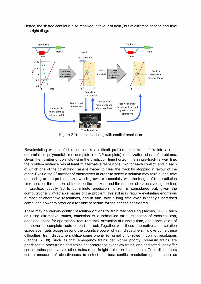
Hence, the shifted conflict is also resolved in favour of train j but at different location and time

(the right diagram).

Figure 2 Train rescheduling with conflict resolution

Rescheduling with conflict resolution is a difficult problem to solve. It falls into a non-

deterministic polynomial-time complete (or NP-complete) optimization class of problems.

Given the number of conflicts (n) in the prediction time horizon in a single-track railway line,

the problem instance has at least 2n alternative resolutions, two for each conflict, and in each

of which one of the conflicting trains is forced to clear the track by stopping in favour of the

other. Evaluating 2n number of alternatives in order to select a solution may take a long time

depending on the problem size, which grows exponentially with the length of the prediction

time horizon, the number of trains on the horizon, and the number of stations along the line.

In practice, usually 30 to 60 minute prediction horizon is considered but, given the

computationally intractable nature of the problem, this still may require evaluating enormous

number of alternative resolutions, and in turn, take a long time even in today’s increased

computing power to produce a feasible schedule for the horizon considered.

There may be various conflict resolution options for train rescheduling (Jacobs, 2008), such

as using alternative routes, extension of a scheduled stop, relocation of passing stop,

additional stops for operational requirements, extension of running time, and cancellation of

train over its complete route or part thereof. Together with these alternatives, the solution

space even gets bigger beyond the cognitive power of train dispatchers. To overcome these

difficulties, train dispatchers utilize some priority (or simplifying) rules in conflict resolutions

(Jacobs, 2008), such as that emergency trains get higher priority, premium trains are

prioritized to other trains, fast trains get preference over slow trains, and dedicated lines offer

certain trains priority over other trains (e.g., freight trains on freight lines). Train dispatchers

use a measure of effectiveness to select the best conflict resolution option, such as

Train j

Train i

Station m -1

Time

Dis

tan

ce

m -2

m +2

m

m +1

m -1

Actual train

movements:

Train j delayed

Prediction

time horizon

Past

Present

Future

Conflict

detected

Conflict

resolution

between train i

and train j

Conflict

resolved in

favor of train j

Train j

Train i

Station m

t t

Trains should

follow planned

tactical schedule

Monitor train

movements

Predict train

movements and

detect conflicts

Resolve conflicts;

line up switches and

signals for actual

operations

t

Train Dispatcher

i

j

minimization of total conflict resolution delay (or total weighted delay based on train

priorities) or maintaining the original schedule as much as possible.

Train rescheduling is performed in a dynamic and evolving environment. It is dynamic

because trains in the dispatching territory continue running while conflict resolution

processes are in progress. The environment evolves because a conflict resolution may

cause some trains to further deviate from their planned schedule and create some other

conflicts, which can adversely affect the schedule adherence totally. The conflict resolution

decisions, therefore, must be made fast and in an efficient manner. So, train dispatchers

should be assisted in their decisions while conducting the rescheduling tasks. Specially

designed decision support systems help dispatchers make efficient and effective decisions in

railway traffic control. The following subsection introduces the basic features of decision

support systems in conjunction with railway traffic control tasks.

2.2 Basics of decision support systems (DSS)

Before introducing the basics of decision support systems, it is beneficial to review the

general decision methodology. Decisions in everyday life are classified into three types:

structured, non-structured and semi-structured. A structured decision gives always the right

outcome by processing the certain set of inputs in a specified way, which can easily be

programmed. On the other hand, a non-structured decision may have several right outcomes

and no precise way to get a right answer (Haag, et al., 1998). A semi-structured decision

falls between the two, involving some of the characteristics of the structured and non-

structured decisions (Turban and Aronson, 1998).

Figure 3 shows the types of decisions in a train dispatching context. If trains operate within

schedule tolerance ranges and there is no any severe disruption, dispatching decisions and

actions are considered to be structured and can be automated based on the planned tactical

schedule. In non-scheduled railways (e.g., some freight railways), improvised traffic control

decisions and actions are taken according to the current circumstances, in which routes are

set and conflicts are resolved manually by train dispatchers. Actual rail operations usually

comprise of semi-structured decisions. For example, if rail traffic adheres to the tactical

schedule in some parts of the dispatching territory, but does not in some other parts,

automated settings are possible for the former, but dispatcher intervention is required for the

latter. Decision support systems are considered to be good at non- and semi-structured

decisions.

There are four phases of decision making, namely intelligence, design, choice, and

implementation (Haag et al., 1998). While normally this sequence is followed in decision

making, modifications are possible with feedback to the previous phases. The following

describes the phases in rail traffic control context:

Intelligence: Find what to fix - Forecast train paths and detect future conflicts;

Design: Find fixes - Search for alternative resolutions of conflicts;

Choice: Pick a fix - Select the best resolution based on measure of effectiveness; i.e.,

total delay, etc.;

Implementation: Apply the fix - Set routes based on the resolution selected.

Figure 3 Types of decisions in train dispatching context

The Information technology behind the rail traffic control DSS brings speed, information and

processing capabilities whilst a train dispatcher as an expert comes with experience,

intuition, judgement, and knowledge. Hence, an implemented DSS provides increased

productivity, understanding, speed, flexibility, and also reduced problem complexity and cost

(Haag et al., 1998).

A generic DSS comprises of three management system components: user interface, DSS

models, and DSS information (Haag et al., 1998). The user interface component (e.g., time-

distance diagrams) allows the user to communicate with the DSS model(s), by which above

mentioned decision phases are represented. It is possible to use various model types in this

component, namely what-if models, optimization models, heuristic models, etc., depending

on the context of rail traffic control problem considered. A DSS receives organizational

information (e.g., rules and regulations), personal information (e.g., manual inputting of traffic

related data received from various sources), and external information (e.g., real-time train

traffic data flowing from field to the dispatching centre) in order to use in model execution

and to provide to the user.

2.3 DSS usage in railway traffic control

Despite some technological developments, the rescheduling process is still heavily under the

manual control of train dispatchers. Some of the implemented decision support systems in

the rail arena help them improve their control capability. One of the pioneering dispatching

support systems was implemented in the US in the early 1980’s, resulting in considerable

annual savings reported, due to reduced train delay, brought about by automatically revising

the routing plans as conditions change (Sauder and Westerman, 1983).

The EUROPTIRAILS project’s main objective is to improve the effectiveness and efficiency

of trains running on European rail corridors by implementing a web interface that can help

reduce delays on international corridors, improve quality of service, optimize the capacity

offer, and communicate the expected time of arrival for customers

(http://www.uic.org/spip.php?article691 accessed on 30 July 2012).

Some trains deviate from schedule out of tolerance

range

Trains adhere schedule within tolerance range

NonNonNon---structured structured structured SemiSemi--structuredstructured Structured

There is no schedule –improvised traffic

control

Both automatic and manual traffic control

Automatic route setting and conflict resolution – recurrent

decisions

Manual route setting and conflict resolution – nonrecurrent, or ad-

hoc, decisions

Decision Support Systems are good at

Another example appears at the DB Netz AG’s operations control centers in Germany. The

manual process of dispatchers is supported by a tool called LeiDis-S/K (Leitsystem

Disposition Strecke/Knoten), which gathers data from the actual operation. The system can

display different diagrams, such as the line/station occupation diagram and time-distance

diagram. It helps dispatchers forecast train movements, detect and resolve conflicts in an

efficient manner (http://fahrweg.dbnetze.com/fahrweg-

en/start/product/ancillary_services/product/controlsystem_leidis_nk.html, accessed on 30

July 2012). Similarly, a computer aided dispatching system at the Union Pacific Railroad in

the US helps dispatchers efficiently and safely route trains

(http://www.unionpacific.jobs/careers/explore/prof/operating/train_dispatcher.shtml#overview

, accessed on 30 July 2012)

3.Rail Terminals Prof. Stefano Ricci, DICEA, Sapienza Università di Roma

3.1 Station layouts: design criteria

The general functions performed by a station are:

Trains stop for loading/unloading;

Trains stop for embarking and disembarking;

Trains stop for crossing and/or overtaking;

Trains stop for shunting and reassembling.

These functions identify the station layouts represented by “Exchange Figures”, also known

as “Müller Figures”, where one Figure can correspond to many layouts. The symbols used

for these figures are synthetically represented by rows linking the lines approaching the

stations, with symbols “O” to identify the possibility for the station to act as terminus for the

concerned line.

Examples of station typologies and the so called Müller Figures are shown in Figures 4 – 6

(reused by Ricci, 2012):

Transit Station

Junction Station

Crossing Station

Figure 4 Layouts I

In the figures below one observes:

Four typological schemes and followed by a schema of transit stations(Juvisy in

France);

Figure 5 Layouts II

Three typological schemes followed by a scheme of terminal station (Roma Termini

in Italy).

Figure 6 Layouts III

The concept of capacity for a station normally corresponds to the maximum number of trains

(Figure 7): a) entering the station, b) performing the planned operation in the station (stops,

overtaking, charge/discharge, manoeuvers, etc.) and c) leaving the station, compatible with a

fixed regularity (punctuality) level. There may be a difference between the theoretical

capacity and the practical capacity depending upon the traffic management (interlocking)

system operated on the concerned station to ensure operational safety.

Figure 7 A Graphical presentation of Capacity

In fact the increase of traffic is progressively causing greater conflicts between trains and

increasing delays, due to the need for trains to wait before they can perform their planned

operation. This leads to a defined maximum amount of waiting time becoming a constraint on

the station capacity.

3.2 Marshalling (Hump) yards: operation and design criteria

Single Wagon (SW) services account for a significant amount of European freight traffic,

although the SW share of global rail freight traffic is gradually decreasing (from 40% in 2005

to approximately 30% in 2010). The concept of SW services is in favour of capillarity and

normally implies that one wagon will form the composition of more than one train, as it

completes its journey from origin to its destination (Rodrigue et al., 2009). These wagons are

normally managed by at least one marshalling yard, where they perform the following

functions:

arrival, check-in, preparation and waiting for the following operations;

classification by departure direction;

ordering by destination station within the same direction;

preparation and waiting for departure, as well as departure itself.

Therefore, the simple operational scheme of a marshalling yard classifying wagons by

gravity using a hump is shown in Figure 8.

Figure 8 A simple graphical presentation of a hump yard

Theoretical capacity with variable trains spacing (e.g.

elastic routes release)

Theoretical Capacity with fixed trains spacing (e.g.

rigid routes release)

Various schemes of yards and their components are shown in Figure 9.

Figure 9 Alternative Yard Schemes

The dimensioning of various yards depends upon different parameters (Figures 10 and 11):

the arrival yard, also known as receiving yard, starting from an expected curve

describing arrivals, characterised by a defined probability σ to be overcome and an

almost deterministic curve of departures through the hump, which can be used for the

estimation of the required number of yard tracks;

the directions yard, also known as classification yard, starting from the number of

lines on which trains are prepared for ordering, a random distribution of arrivals at

classification yard from the hump, followed by planned departures;

the ordering and departure yard starting from the number of lines on which trains are

prepared for departure, the number of destinations along each line, a planned

distribution of arrivals at departure yard, followed by procedures and rules for train

departure, which are dictated by the production pattern in operations (a strict fixed

schedule and/or improvised operation).

Figure 10 Curves describing arrivals and departures at/from arrival yard

Figure 11 Showing train departures from a yard; Improvised Operation

A different approach allows the dimensioning of the yard hump, which includes both

geometrical morphology and energy need to reach the end of direction yard tracks by all

wagons typologies and under any environmental condition (Figures 12 and 13).

Figure 12 A graphical presentation of a hump profile I

Figure13 A graphical presentation of a hump profile II

The capacity (nmax) of the marshalling yard is identified by the capacity of its bottleneck, i.e.,

the yard hump and can be estimated using the formula (5.1).

(5.1)

, where:

T is the reference time;

t3 and t4 are operational breaks due to maintenance and accidental events;

nct is the average number of wagons per section (with the same destination station);

lt is the section length;

vm is the average section speed;

∆t is the minimum headway between sections;

Xmv are the loco manoeuvring parameters.

3.3 Intermodal terminals: operation and design criteria

Combined transport, formed of a combination of different transport modes, requires the

management of transport units by intermodal terminals for modal shift (Figures 14 and 15). A

fully intermodal terminal includes water, rail and road transport systems (Malavasi, Ricci,

2010) and allows transfer for both intra-modal and inter-modal units, stocking of units and

additional services (e.g. commercial) with added value. What one observes in reality is that

partial terminals with a reduced set of functions are often operated.

The typical intermodal transport units (Figure 14) are:

Container, with standard dimensions (ISO 1/2/3), standard weight, possible

overloading (max 5 units) and standard spreaders;

Swap body, with standard dimensions (4 typologies), but no overloading;

Pallet, with standard dimensions (ISO A/B/C/D);

Semi-trailer, with dimensions defined by road traffic admission, trailed by trucks and,

therefore, chargeable by Ro-Ro mode.

Figure 14 Units of combined transport

The typical equipment used to transport units in terminals (Figure 15) includes:

Portainer, operating from ship to land and v.v.;

Straddle carrier, operating in stocking areas;

Transtainer, operating on rails or rubbers over stocking areas, tracks and roads;

Fork lift, operating in/to stocking areas with high manoeuvrability;

Reach stacker, operating in/to stocking areas with high visibility;

Semitrailer, operating in/to stocking areas for transport only, but with higher speed.

Figure 15 Equipment for Loading/Unloading

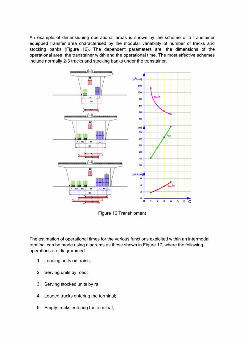
An example of dimensioning operational areas is shown by the scheme of a transtainer

equipped transfer area characterised by the modular variability of number of tracks and

stocking banks (Figure 16). The dependent parameters are: the dimensions of the

operational area, the transtainer width and the operational time. The most effective schemes

include normally 2-3 tracks and stocking banks under the transtainer.

Figure 16 Transhipment

The estimation of operational times for the various functions exploited within an intermodal

terminal can be made using diagrams as these shown in Figure 17, where the following

operations are diagrammed:

1. Loading units on trains;

2. Serving units by road;

3. Serving stocked units by rail;

4. Loaded trucks entering the terminal;

5. Empty trucks entering the terminal;

6. Trucks in/out .

Figure 17 A Graphical presentation of terminal operations

4 Time-tabling Gordana Vasic-Franklin, NewRail, Newcastle University

4.1 Activities for creating a timetable

Timetable creation includes several modelling processes and datasets that are incorporated

and intertwined:

Calculating demand;

Infrastructure modelling;

Running time calculation;

Train paths modelling ;

Timetable simulations;

Optimisation modelling;

Rolling stock datasets;

Rolling stock and staff planning.

4.2 Demand

Passenger demand Passenger needs change according to location and time. If people live in rural areas,

frequency of trains during the day is low, while city stations have a high frequency of trains.

Demand changes with time of day, time of year, etc., as shown in Table 2. Basic

characteristics and data of passenger flows (number of passengers that in specified time

period travel between two stations on a line, (Bankovic, 1994)) are acquired in various ways,

but usually through counting of passengers and questionnaires. That gives, for each time

period, the expected maximum passenger flow on each line, which serves as authoritative

for calculating the required rolling stock capacity and the selection of train paths.

Table 2 Passenger demand variation with time period

Year Week Time of day

Summer Monday to Friday Commute morning

Winter Saturday Mid-day

Sunday Commute

afternoon Holidays Evening

Night

Freight demand Freight transport scheduling depends on the type of goods that are transported. Demand for

transport of agricultural products, for example, would have a known seasonal variation,

whereas ore from mines and quarries would be less variable. In addition, organic produce

needs to be delivered quickly to avoid spoiling, whereas ore transport (and freight generally)

is less time-critical.

Commodities are transported from ports, mines, industrial centres, consolidation centres,

etc., and could be cross-border shipments. Having a classical timetable is not practical, so

trains are run on-demand. This could be either by running freight trains daily in pre-

scheduled on-demand paths in yearly timetables or running freight trains as ‘extra’ trains.

This means that the freight operator could request a train path for an extra train on the rail

network, just a few hours in advance, which gives more optimised transport.

4.3 Infrastructure modelling

Infrastructure consists of: tracks, signals, telecommunications and catenary. It can be

modelled using nodes (representations of a location) and links (connections between two

nodes). Depending on whether the network needs to be presented in more detail

(‘microscopic’) or less (‘macroscopic’), nodes and links hold slightly different information. In

the macroscopic model, nodes will have information about the following attributes: name,

coordinates, type (station, shunting yard, junction, etc.); and links will have information on:

length, type of line (high speed, passenger, freight or mixed), number of tracks, average

running time, average capacity. In the microscopic model, node type would be signal, point,

etc., and links would hold more detailed information: gradient, permissible speed, curve

radius, etc. For example, a station in a macroscopic model is just one node, but in a

microscopic model it would be an aggregate of hundreds of nodes and links, depending on

complexity (Figure 18). Note that for calculating running times, creating timetables and

simulations, a microscopic model is required.

Figure 18 Top: Microscopic representation of station as an aggregate of nodes and links.

Bottom: Macroscopic basic node-link-node structure.

4.4Running time calculation

Running time is calculated for each train configuration and for specific, current infrastructure,

and is necessary for creating timetables. Running time depends on characteristics of:

- Infrastructure: length, gradients, curves, tunnels, permissible speed.

- Traction unit (e.g., locomotive): tractive effort and resistance.

- Rolling stock: mass, length, resistances.

- Operating cycle: starting point, stops (e.g., stations, signals).

The route is divided into sections with specific dynamic behaviours, i.e., acceleration,

constant movement and braking sections that have the same characteristics and operational

behaviour. A time calculation is then made, using appropriate formulae for each section,

taking into account available tractive effort, braking requirements, and rolling and

aerodynamic resistances.

Train spacing, signalling and headway Another important thing for the timetable planner is to make sure that there is enough

separation between trains. On all networks, separation is achieved through signalling, and

the separation distance depends on the type of signalling (2, 3 or 4 aspect signalling). In an

example of 3-aspect signalling, trains must be separated by two signal sections, plus the

length of the first train and the length of the overlap of the red signal (Figure 5.19). Time

between trains will be dependent on the separation distance and their speed.

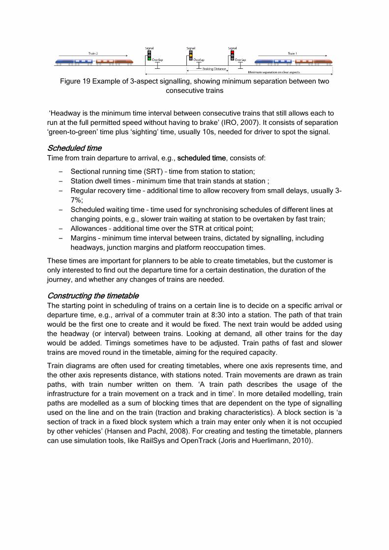
Figure 19 Example of 3-aspect signalling, showing minimum separation between two

consecutive trains

‘Headway is the minimum time interval between consecutive trains that still allows each to

run at the full permitted speed without having to brake’ (IRO, 2007). It consists of separation

‘green-to-green’ time plus ‘sighting’ time, usually 10s, needed for driver to spot the signal.

Scheduled time Time from train departure to arrival, e.g., scheduled time, consists of:

– Sectional running time (SRT) – time from station to station;

– Station dwell times – minimum time that train stands at station ;

– Regular recovery time – additional time to allow recovery from small delays, usually 3-

7%;

– Scheduled waiting time – time used for synchronising schedules of different lines at

changing points, e.g., slower train waiting at station to be overtaken by fast train;

– Allowances – additional time over the STR at critical point;

– Margins – minimum time interval between trains, dictated by signalling, including

headways, junction margins and platform reoccupation times.

These times are important for planners to be able to create timetables, but the customer is

only interested to find out the departure time for a certain destination, the duration of the

journey, and whether any changes of trains are needed.

Constructing the timetable The starting point in scheduling of trains on a certain line is to decide on a specific arrival or

departure time, e.g., arrival of a commuter train at 8:30 into a station. The path of that train

would be the first one to create and it would be fixed. The next train would be added using

the headway (or interval) between trains. Looking at demand, all other trains for the day

would be added. Timings sometimes have to be adjusted. Train paths of fast and slower

trains are moved round in the timetable, aiming for the required capacity.

Train diagrams are often used for creating timetables, where one axis represents time, and

the other axis represents distance, with stations noted. Train movements are drawn as train

paths, with train number written on them. ‘A train path describes the usage of the

infrastructure for a train movement on a track and in time’. In more detailed modelling, train

paths are modelled as a sum of blocking times that are dependent on the type of signalling

used on the line and on the train (traction and braking characteristics). A block section is ‘a

section of track in a fixed block system which a train may enter only when it is not occupied

by other vehicles’ (Hansen and Pachl, 2008). For creating and testing the timetable, planners

can use simulation tools, like RailSys and OpenTrack (Joris and Huerlimann, 2010).

Figure 20 Time-distance diagram.

Station timetables are created by separate models, where each train that arrives has to be

assigned to an appropriate platform and corresponding inbound and outbound routes. Figure

5.20 shows a time-distance diagram.

Example 1 – Scheduling trains on a line The simplest way to understand creation of timetables is with the example of a train line with

known turnaround time and intervals. Consider Figure 5.21. Turnaround time T0 is the time

that one train set needs to complete the full cycle, from its first to the next departure from the

same terminus (an end station).

The red line in the graph is the train path of the first fixed train. It doesn’t include stops at

each station, only waiting at each terminus for simplicity, because the aim of this example it

to see how you include trains in the schedule. The train starts at Terminus A at 4.00. It

arrives at Terminus B at time 5.50. The train then goes back to Terminus A and continues

until it stops working at time 22.50. The 2nd train starts from Terminus A after the set interval

of 1h, at time 5.00. Intervals are not the same through a day, they increase during off-peak

times, i.e., fewer trains are needed during the afternoon and late evening, and none run

during the night.

Figure 21 Graphical representation of timetable construction. Red line – movement of the first

fixed train from Station A; The four trains operating on the route are represented with

different colours. T0 – turnaround time.

Capacity “The Capacity of a railway is its maximum possible usage, that is, the number of trains that

could run, regardless of demand and resources. Utilisation is then the actual Usage

expressed as a percentage of the Capacity” (IRO, 2007). Capacity is often defined as “trains

per hour”, and it is 60min divided by the headway. The reason to calculate capacity is to see

what is the maximum number of trains that could be run, when doing the new timetable or

checking how efficient the timetable is, e.g. how well the line is utilised. The full capacity is

only used if there is a sufficient demand for it.

Staff and rolling stock planning and utilisation After timetable is created, the next step is to plan trains and staff:

Allocate vehicles to trains in the timetable:

o For passenger trains it depends on the demand of peak trips (but don’t run the

peak number of trains all day if at all possible);

o For freight trains it depends of allowed routes they can use, because of axle-

load and gauge clearance.

Fuelling for diesel trains and restrictions of electrification have to be taken into

account

The aim is to finish the day’s work at or close to, the maintenance location.

When creating crews diagrams, the following has to be taken into consideration:

Crews work in shifts, round 8 hours a day;

Think of appropriate crew changeovers;

Think about breaks within the shift and allowed continuous driving time without a

break;

(Drivers must have route and traction knowledge);

Holidays.

Access rights and bids Each European country has its own rules and regulations about timetable planning. Most

European countries have split rail responsibilities between infrastructure and train operators.

They operate on a commercial basis where infrastructure companies sell train paths to

operating companies. In Great Britain “Each train operator has a contract (“an access

agreement”) with Network Rail, (infrastructure owner/manager) in which trains they are

entitled to run are defined” IRO, 2007. Freight operators run their extra trains using “spot bid”

when they need to add or amend a path in the permanent timetable.

5 Rail Network Policy Dr. Marin Marinov, NewRail, Newcastle University

5.1 Service, Components and Bottlenecks

Rail operators provide a “network-based” service, which requires a rail network policy.

Railways serve many passengers daily and transport massive quantities of freight using a

limited number of static and dynamic resources. To provide a good standard of service at low

cost, network evaluation methods should be used to evaluate, plan and optimise the levels of

rail system performance.

Network evaluation methods include service network design, gravity models, queuing

networks, simulations and optimising network models. For the purposes of the analysis, the

rail network being studied might be divided into its components such as rail lines, railway

stations, yards, terminals interchanges, etc. This way, the performance of each component

can be analysed separately in detail.

Rail network operation, however, is interconnected and dependent on the performance

levels of each component. Each component is characterised by arrival process, service

pattern and departure process. The arrival process is characterised by an arrival rate and

specifies the frequency and the number of trains to arrive in a given component over a

certain period of time. The service pattern is the rate at which trains are served by a given

component. The departure process is characterised by a departure rate and specifies the

frequency and the number of trains to depart from a given component over a certain period

of time.

In complex serial networks like rail networks, one component’s departure process dictates

the next component’s arrival process and therefore network components should not be

examined in isolation. In many cases the quality of the service provided is dependent on the

performance of the component with the lowest processing capacity, this is known as the

bottleneck. To identify the bottlenecks of a network, the Fluid Model can be applied (Hall,

1991, pp. 352).

To avoid the bottleneck phenomenon rail networks should be designed so that the

component processing capacities are identical to the greatest extent possible.

5.2 Service Network Design

Service Network Design is to provide such a layout that ensures easy train movement and

avoids congestions. In the cases where there is a specific client demand, service network

design is to generate one better way to serve this demand subject to the physical

characteristics of the existing network. Specifically, we look for decisions that optimise the

selection of physical routes, production pattern, speed, service frequency and the like.

The physical configuration of the rail network is of significant importance. Loading/unloading

terminals, yards, stations and interchanges should be designed so that they are convenient

to rail operators and customers, whilst minimising waiting times and avoiding delays.

The physical network is usually represented by a directed/oriented graph which consists of

nodes and arcs. The nodes represent all the loading and unloading terminals, yards,

interchanges, junctions, stations and rail crossings. The arcs represent all the links

connecting all the nodes in the rail network. A graphical representation of the network as an

oriented graph visualises all the possible demand Origin/Destination pairs in the network. For

example an oriented two directional graph with nine nodes and twenty six arks is shown in

Figure 22.

Figure 22 Oriented Two Directional Graph.

All the nodes and arcs are defined by the service pattern, standing and processing capacity

as well as costs for service. Demands for every Origin/Destination pair are given in advance.

There may be other requirements, such as: priorities; strict fixed routes for some of the

freight flows; schedules as well as working hours. All these requirements the development of

a realistic model a difficult proposition, therefore a combination of methods should be

employed when designing services in rail networks.

Optimising network models help to schedule an effective service in complex busy networks.

More specifically optimising network models are employed with the aim to define an optimal

routing of the moving assets in the network with respect to some objective function for

instance minimising overall costs for service, minimising waiting times of the moving assets,

maximising network utilization or minimising the throughput time and the time for service.

Complex rail networks serve heterogeneous mixed traffic, meaning that different categories

of trains (both freight and passengers) are operated on the same network, running on the

same lines. Passenger trains run on strict fixed timetables, although freight trains may have

different behaviour than passenger trains. It is a usual practice for freight trains to run on

improvised schemes, meaning that freight trains are held in rail yards until they are full,

meaning that they reach the train length limit and maximum weight (payload plus tare) as

specified by the technical characteristics of the rail network.

Repetitive regrouping of freight wagon groups into freight trains is a typical for the orthodox

rail freight system. This operation is carried out in rail freight yards. The system is also

characterised by a very significant non-linearity of costs for transport due to the necessity of

a road locomotive. Variability in demand sometimes forces the system to experience

undesirable levels of underutilisation. On the other hand to fulfil a strict fixed schedule in a

network, road locomotives may have to run even if they are only moving a few freight

wagons. The process of designing and analysing an operating process with freight trains in a

network might not be easy. Usually this analysis begins with how the rail freight network in

question can be transformed into a promising shape for the analysis.

Auxiliary networks can be implemented to study the behaviour of a component of the rail

network. Rail yard operations, for instance can be studied using queuing networks of a

known shape. Jackson (1957) defined sufficient conditions under which a queuing network

can be divided into individual M/M/m systems with characteristics as follows:

-M/M/1 - exponential inter-arrival times, exponential service times, one server, infinite

buffer capacity;

-M/M/m - exponential inter-arrival times, exponential service times, m servers, infinite

buffer capacity;

-M/M/m b - exponential inter-arrival times, exponential service times, m servers, fixed

buffer size.

Jackson conditions include: Poisson arrivals, independent and exponential service times,

infinite buffer capacity, independent discipline of customer routing and service times, a fixed

probability transfer matrix defines customer routing. Although restricted in application

Jackson networks yield promising results when used to analyse and design rail service

networks.

A Queuing network analyser can be utilised to study the behaviour of a rail network

component such as a rail passenger station, a marshalling yard, a stabling yard, a

locomotive shed, and such like, if this particular component can be described as part of a

queuing network. A Queuing network analyser employs G/G/m queuing systems and can be

implemented to study any type of queuing network. G/G/m queuing systems employ general

distributions, meaning that any service time distribution that is independent of the state and

the inter-arrival times can be implemented to describe any particular component of a queuing

network.

It should be noted that G/G/m queuing systems use approximations, and the accuracy of the

results depends strongly on the calculation of the coefficient of variation of the inter-arrival

time. For example formula 5.2 is the Allen and Cunneen approximation for m = 1 to calculate

expected number of customers in queue (Hall 1991, pp 153).

2

)()(*

221//1// SCAC

LL MM

q

GG

q (5.2)

, where

LqM/M/1- the expected numbers of customers in queue for queueing system M/M/1, i.e.:

1

21// MM

qL , ρ < 1 (5.3)

, where

ρ – absolute utilisation of the system, this is the average number of servers

that are busy over time;

C(A) – coefficient of variation of the inter-arrival times;

C(S) – coefficient of variation of the service times;

2

)()( 22 SCAC - an adjustable factor.

Formula 5.4 is the Allen and Cunneen approximation for m = 2:

21

*2

)()(*

21

222

2

//

SCACL mGG

q , ρ < 2 (5.4)

, where

ρ – absolute utilisation of the system, i.e. the average number of servers that

are busy over time;

C(A) – coefficient of variation of the inter-arrival times;

C(S) – coefficient of variation of the service times;

21

*2

)()( 22

SCAC - an adjustable factor.

5.3 Simulation modelling for analysing rail networks

Simulation modelling has been employed by the rail industry to study the current level of

efficiency and the capacity of the railway networks. Simulation modelling has also been

implemented to evaluate the alternative scenarios for the implementation of a new network-

wide policy, for instance, building a new line and/or a terminal, implementation of a new

schedule, alternative production schemes and the like.

Simulation models operate with comprehensive data input which includes a set of rules and

properties to describe properly and realistically the rail infrastructure, itineraries, arrival

service and departure patterns, schedules, behaviour of moving assets, interruptions,

disruptions, etc. Statistical methods are employed to analyse the output of simulation models

and make decisions.

Software packages specifically developed to simulate rail networks are for instance: RailSys,

OpenTrack and ERSA Traffic Simulators. If such a specific software package is not

available, even-based simulation tools can be implemented to simulate rail networks and

their components.

Dessouky and Leachman (1995) used SLAM II Simulation Language to study complex rail

networks. Their work has been further extended by Dessouky et al. (2002) and Lu et al.

(2004) who developed simulation modelling methodologies for assessing the rail

infrastructure in dense traffic areas.

García and García (2012) have used Witness to study configurations of rail infrastructure and

intermodal services. Woroniuk and Marinov (2012) have developed simulation models to

study the utilisation levels of rail corridors using ARENA. Marinov and Viegas (2009,

2011a,b,c) have developed simulation modelling methodologies to study operating

processes with freight trains in rail freight yards and in a network using SIMUL8. These

methodologies have been implemented for the needs of a rail freight operator, and more

specifically improvised vs. scheduled rail freight network operations have been studied. The

simulation models demonstrate that: a scheduled rail freight network operation is

characterised by lower queue sizes, lower operating costs for the rail freight operator, a

higher number of freight trains being served, a better level of capacity utilisation is achieved

and hence the network operation is more profitable; the more deviations from the schedule,

the more delays in the network, the larger the queue size, the less useful work, the higher the

operating costs, the greater the diseconomy of scale.

References

Anthony, R., 1965. Planning and Control Systems: A Framework for Analysis, Harvard

Graduate School of Business, Boston

Assad, A., 1980. Models for Rail Transportation, Transportation Research Part A: General,

Vol. 14, Issue 3, June 1980, Pages 205-220, Printed in Great Britain

Ballis, A. and Golias, J., 2004. Towards the Improvement of a Combined Transport Chain

Performance, European Journal of Operational Research 152, 420 - 436

Bankovic, R., 1994. Organizacija i tehnologija javnog gradskog putnickog prevoza

[Organization and technology of public passenger transport], Beorgad, Sluzba za izdavacku

delatnost Saobracajnog fakulteta

Crainic, T., Ferland, J., and Roussean, J., 1984. A Tactical Planning Model for Rail Freight

Transportation, Transportation Science, Vol. 18, No. 2

Crainic, T. and Roy, J., 1988. O.R. tools for tactical freight transportation planning, European

Journal of Operations Research, Vol. 33, No. 3

Crainic, T. and Laporte, G., 1997. Planning Models for Freight Transportation, European

Journal of Operations Research, Vol. 97, Issue 3

Dessouky, M., and Leachman, R., 1995. A Simulation Modeling Methodology for Analyzing

Large Complex Rail Network, Simulation, Vol. 65, No. 2

Dessouky M., Lu Q. and Leachman R., 2002. Using Simulation Modeling to Assess Rail

Track Infrastructure in Densely Trafficked Metropolitan Areas, Proceedings of the 2002

Winter Simulation Conference, E. Yücesan, C.-H. Chen, J. L. Snowdon, and J. M. Charnes

García, A. and García, I., 2012. A simulation-based flexible platform for the design and

evaluation of rail service infrastructures Simulation Modelling Practice and Theory 27 (2012)

31–46

Gualda, N. and Murgel, L., 2000. A Model for the Train Formation Problem, RIRL-Les

Troisiemes Rencontres internationals de al Recherche en Logistique Trios-Rivieres, May 9,

10 and 11

Haag, S., Cummings, M., Dawkins, J., 1998. Management Information Systems for the

Information Age. Irwin McGraw-Hill Companies, Inc., USA, pp. 162-207.

Hall, R., 1991, Queuing Methods for Services and Manufacturing, University of California at

Berkeley, Prentice Hall International,Inc., ISBN 0-13-748112-8

Hansen, I. and Pachl, J. eds., 2008. Railway timetable & traffic. Analysis. Modelling.

Simulation. Hamburg: Eurailpress.

Jacobs, J., 2008. Rescheduling. In: Hansen, I.A., Pachl, J. (Eds.) Railway Timetable & Traffic

– Analysis, Modelling, Simulation, Eurailpress, DW Rail Media, Hamburg, Germany, pp. 182-

191.

Jackson J., 1957. Networks of Waiting Lines, Operations Research, Vol. 5

Joris, P., and Huerlimann, D., 2010. OpenTrack - Simulation of Railway Networks, Open

track slides, IT10 RAIL

Lu Q., Dessouky M. and Leachman R., 2004. Modeling Train Movements Through Complex

Rail Networks, ACM Transactions on Modeling and Computer Simulation, Vol. 14, No. 1

Malavasi G., Ricci S., 2010. Dispense del Corso di Trasporti Marittimi – Sapienza Università

di Roma, Dicembre 2010 (http://w3.uniroma1.it/stefano.ricci/mat_didattico.html)

Marinov M, and Viegas J., 2009. A simulation modelling methodology for evaluating flat-

shunted yard operations, Simulation Modelling Practice and Theory 2009, 17(6), 1106-1129

Marinov, M. and White, T., 2009. Rail Freight Systems: What Future?. World Transport

Policy & Practice 2009, 15(2), 9-28.

Marinov M, and Viegas J., 2011a. A Mesoscopic Simulation Modelling Methodology for

Analyzing and Evaluating Freight Train Operations in a Rail Network. Simulation Modelling

Practice and Theory 2011,19 516-539.

Marinov, M., and Viegas, J., 2011b. Analysis and Evaluation of Double Ended Flat-shunted

Yard Performance Employing Two Yard Crews. Journal of Transportation Engineering 2011,

137(5), 319-326.

Marinov, M., and Viegas, J., 2011c. Tactical management of rail freight transportation

services: evaluation of yard performance. Transportation Planning and Technology 2011,

34(4), 363-387.

Miles, R., 1975. Theories of Management: Implications for Organizational Behavior and

Development, McGraw Hill Text

Mücke, W., 2002. Operations Control Systems in Public Transport. Eurailpress Tetzlaff-

Hestra GmbH & Co. KG, Germany.

Pachl, J. and White, T., 2003. Efficiency through Integrated Planning and Operation,

International Heavy Haul Association, Virginia Beach

Ricci S., 2012. Dispense del Corso di Trasporti Ferroviari – Sapienza Università di Roma,

Aprile (http://w3.uniroma1.it/stefano.ricci/mat_didattico.html)

Rodrigue, J.P., Comtois, C., Slack, B., 2009. The Geography of Transport Systems,

Routledge. New York, ISBN 978-0-415-48324-7

Sauder, R.L., Westerman, W.M., 1983. Computer aided train dispatching: decision support

through optimization. Interfaces 13(6), 24-37.

Taylor, F., 1911, Principles of Scientific Management, Harper & Row

The Institution of Railway Operators, 2007. Train planning & performance management,

Course material.

Turban, E., Aronson, J.E., 1998. Decision Support Systems and Intelligent Systems. Fifth

Edition, Prentice-Hall International, Inc., USA.

Watson, R., 2001. Railway scheduling. In: Button, K.J., Hensher, D.A., (Eds.), Handbook of

Transportation Systems and Traffic Control, Elsevier Science, Ltd., UK, pp. 527-538.

White, T., 2003. Elements of Train Dispatching. Volume 2 Handling Trains, VTD Rail

Publishing, USA.

Woroniuk, C., Marinov, M., 2012, Simulation modelling to analyse the current level of

utilisation of sections along a rail route. Revista de Literatura dos Transportes 2012, 7(2). In

Press.

Web sources

http://www.belfasttelegraph.co.uk/news/local-national/uk/rail-punctuality-shows-

improvement-16143933.html, accessed on 25 June 2012

http://www.zssk.sk/sk/passenger-rights , accessed on 25 June 2012

http://europa.eu/youreurope/citizens/travel/passenger-rights/rail/index_en.htm , accessed on

25 June 2012

http://www.trainrefunds.co.uk/ , accessed on 25 June 2012

http://en.wikipedia.org/wiki/Rail_transport_in_Japan , accessed on 25 June 2012

http://europa.eu/legislation_summaries/transport/rail_transport/l24075_en.htm ,accessed on

25 June 2012

http://www.uic.org/spip.php?article691 ,accessed on 30 July 2012

http://fahrweg.dbnetze.com/fahrweg-

en/start/product/ancillary_services/product/controlsystem_leidis_nk.html ,accessed on 30

July 2012

http://www.unionpacific.jobs/careers/explore/prof/operating/train_dispatcher.shtml#overview

, accessed on 30 July 2012

www.opentrack.at , accessed on 30 July 2012

www.rmcon.de , accessed on 30 July 2012

www.networkrail.co.uk , accessed on 30 July 2012