no-treatment-e ect hypothesis in a comparative experiment1

A Closer Look at Testing the “No-Treatment-Effect”

Hypothesis in a Comparative Experiment1

Joseph B. Lang

Department of Statistics and Actuarial ScienceUniversity of Iowa, Iowa City, IA USA

Abstract

Standard tests of the “no-treatment-effect” hypothesis for a comparative experiment includepermutation tests, the Wilcoxon rank sum test, two-sample t tests, and Fisher-type randomiza-tion tests. Practitioners are aware that these procedures test different no-effect hypotheses andare based on different modeling assumptions. However, this awareness is not always, or evenusually, accompanied by a clear understanding or appreciation of these differences. Borrowingfrom the rich literatures on causality and finite-population sampling theory, this paper developsa modeling framework that affords answers to several important questions, including: exactlywhat hypothesis is being tested?, what model assumptions are being made?, and are thereother, perhaps better, approaches to testing a no-effect hypothesis? The framework lends itselfto clear descriptions of three main inference approaches: science-based, randomization-based,and selection-based. It also promotes careful consideration of model assumptions and targetsof inference, and highlights the importance of randomization. Along the way, Fisher-typerandomization tests are compared to permutation tests and a less well known Neyman-typerandomization test. A small-scale simulation study compares the operating characteristics ofthe Neyman-type randomization test to those of the other more familiar tests.

Keywords and Phrases: Causal effects; Completely randomized design; Finite-population sam-pling theory; Fisher vs. Neyman; Fisher’s exact test; Horvitz-Thompson estimator; Non-measurable probability sample; Permutation tests; Potential variables; Randomization-basedinference; Randomization tests; Science-based inference; Selection-based inference

1 Introduction

We begin with a simple example of a comparative experiment. Researchers are interested in de-

termining whether cell phone use while driving has an impact on reaction times. Toward this end,

64 University of Utah student volunteers were enlisted to take part in a randomized comparative

experiment (Strayer and Johnston 2001). Of the 64 students, 32 were randomized to treatment 1

(operate a driving simulator while using a cell phone) and 32 were randomized to treatment 2

(operate a driving simulator without a cell phone). For a summary description of the data and of

the way the two treatments were actually administered, see Agresti and Franklin (2007:446). In the

driving simulation, each student encountered several red lights at random times. Each student’s

response was the average time required to stop when a red light was detected. The 64 responses,

in milliseconds, are recorded in Table 1.

11/25/12 This research was supported in part by NSF grant SES-1059955.

A Closer Look... 2

Table 1. Reaction Times (milliseconds).

Cell Phone: 636 623 615 672 601 600 542 554 543 520 609 559 595 565 573 554

626 501 574 468 578 560 525 647 456 688 679 960 558 482 527 536

Control: 557 572 457 489 532 506 648 485 610 444 626 626 426 585 487 436

642 476 586 565 617 528 578 472 485 539 523 479 535 603 512 449

Generically...Treatment 1: y1,1, y1,2, . . . , y1,32

Treatment 2: y2,1, y2,2, . . . , y2,32

Is there a cell phone use effect? Generically, is there a treatment effect?

Standard tests of the “no-treatment-effect” hypothesis include permutation tests (Pitman 1937,

1938), the Wilcoxon rank sum test (Wilcoxon 1945), two-sample t tests (cf. Welch 1938), and Fisher-

type randomization tests (Fisher 1935). Most practitioners are aware that these procedures test

different “no-effect” hypotheses and are based on different modeling assumptions. However, this

awareness is not always, or even usually, accompanied by a clear understanding or appreciation

of these differences. This paper looks at each of these testing approaches and addresses the all

important questions, exactly what hypothesis is being tested? and what model assumptions are

being made? Along the way, we will have to confront several other questions such as, how is the

definition of treatment effect operationalized?, what is the actual target of inference?, what is

the role of randomization?, and are there other, perhaps better, approaches to testing a no-effect

hypothesis?

To address these questions, we draw on ideas from the rich literature on causal analysis. In

particular, we employ the useful concept of “potential variables.” Although the idea of potential

variables can be traced back to Neyman (1923), Rubin, begining with a series of papers on causal

models in the 1970’s (see Rubin 2010 and references therein) is usually credited with more explic-

itly stating the potential variable model and extending it to both randomized and non-randomized

design settings, with or without covariates (see Rubin’s causal model, Holland 1986). Between Ney-

man and Rubin, potential variables were used by relatively few authors; Welch (1937), Kempthorne

(1952, 1955), and Cox (1958) were among the notable early proponents. Around the time of and

after Rubin, many more authors made important contributions to the potential variables literature.

See for example, Copas (1973), Holland (1986), Greenland (1991, 2000), Gadbury (2001), and the

references therein.

To be clear, it is not the goal of this paper to summarize the vast literature on potential variables

and causal modeling. (To this end, see Paul R. Rosenbaum’s very informative website and references

therein, www-stat.wharton.upenn/ rosenbap/downloadTalks.htm.) Instead, the first goal is to

exploit the benefits of hindsight to develop a modeling framework that supports clear descriptions

and comparisons of the different testing approaches, and promotes careful consideration of the

model assumptions and targets of inference. This modeling framework and associated notation

draws clear distinctions between realizations and random variables, and between observed and

unobserved data. It accommodates both treatment assignment and sampling from populations, and

clearly differentiates between the two. Although the proposed model lends itself to generalizations

A Closer Look... 3

in many directions (e.g. more than two treatments, restricted randomization, etc.), to simplify

exposition, we will focus on the two-treatment comparative experiment setting. This restriction

allows us to more directly highlight the useful features of the proposed modeling framework.

The second goal of this paper is to address the question of availability of other testing ap-

proaches, besides the four common ones mentioned above. Toward this end, we revisit ideas in-

troduced in Neyman (1923). Using the model structure introduced herein, we describe a less well

known Neyman-type randomization test, which is qualitatively different than the Fisher-type ran-

domization test (cf. Welch 1937, Rubin 1990, 2004, 2010).2 The Neyman-type randomization test,

which uses a less restrictive “no-effect” hypothesis than Fisher’s, is based on a test statistic with the

common form, (estimator minus estimand)/(standard error of estimator). Neyman, with an eye on

interval estimation rather than testing, derived the standard error with respect to a randomization

distribution using tools from finite-population sampling theory. In retrospect, Neyman’s derivation

approach is hardly surprising given that he “may be said to have initiated the modern theory of

survey sampling” (Lehmann 1994) in his landmark paper of 1934 (Neyman 1934). Compared to

Fisher-type randomization tests, the Neyman tests do have their advantages and disadvantages.

One disadvantage is that Neyman tests are approximate, whereas Fisher tests are exact. An ad-

vantage is that the Neyman test can be more powerful than the Fisher test (see section 10 below).

Another advantage is that, unlike the Fisher-type randomization test, the Neyman version can be

used to test hypotheses about a population when units are randomly sampled from the population

and then randomized to treatment levels.

The third and final goal of this paper is to compare the operating characteristics of the five

tests: the permutation test, the Wilcoxon rank sum test, the two-sample t-test, the Fisher-type

randomization test, and the Neyman-type randomization test. The penultimate section of the

paper includes a small-scale simulation study of the size and power of these five tests. Based on

these comparisons, we make tentative recommendations on which test to use in different settings.

The remainder of this paper is organized as follows: Section 2 introduces potential variables

and recasts the data in Table 1 within this framework. Section 3 introduces a sequential data

generation model that explicitly accommodates both random sampling and randomization. The

components in the three-level sequential model are identified as the “science,” the “sampling,” and

the “randomization.” This model, along with a useful component-selection notation, leads to an

explicit identification of the observed data and the three main targets of inference. Section 4 gives

candidate definitions of treatment effects that are based on potential variables, along with corre-

sponding no-treatment-effect hypotheses. An overview of the three main inference approaches—

science-based, selection-based, and randomization-based—is given in Section 5 and candidate test

statistics corresponding to these inference approaches are given in Section 6. Sections 7-9 describe

each of the three inference approaches in more detail. These sections give specific examples of

testing procedures, some of them well known and some of them less well known. Section 10 carries

out an analysis of the cell phone data and includes a small scale simulation study of the operating

2Readers with an interest in history are encouraged to read Neyman (1935), along with the discussions, to seehow Neyman and Fisher publicly aired their differences of opinions on testing in randomized design settings.

A Closer Look... 4

characteristics of the different testing approaches discussed herein. Finally, Section 11 includes a

brief discussion.

2 What Might Have Been: The Potential Variables Viewpoint

Going back to Neyman (1923) and following the lead of Welch (1937), Kempthorne (1955), Cox

(1958), and Rubin (e.g. 2005), we will view the data as observed values of a sample of “potential

values.”

Consider a population P of N units that are, without loss of generality, identified by the

numbers 1 through N ; in symbols, P = (1, . . . , N). Let Yt.i be the response for unit i when exposed

to treatment t, where i = 1, . . . , N and t = 1, 2. The response variables Y1.i and Y2.i are called

potential variables for reasons made clear in the next paragraph.

The introduction of these potential variables leads to intuitively appealing definitions of treat-

ment effects that are based on head-to-head comparisons of Y1.i and Y2.i. There is a catch, however.

Although there is the potential to observe either Y1.i or Y2.i, unfortunately, it is not possible to

observe both. Strictly speaking, it is not possible to observe the values of both potential variables

because the same subject cannot be simultaneously exposed to both treatments. To the potential

variable advocates, this is the “fundamental problem of causal analysis” (Holland, 1986). As an

example, if we observe the value of Y2.i, then the value of Y1.i, and hence the difference Y1.i − Y2.i,

cannot be observed. In this case, the unobserved value of Y1.i is relegated to fantasy, the value is

“what might have been” had unit i been exposed to treatment 1 rather than treatment 2.

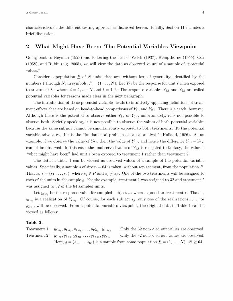
The data in Table 1 can be viewed as observed values of a sample of the potential variable

values. Specifically, a sample s of size n = 64 is taken, without replacement, from the population P .

That is, s = (s1, . . . , sn), where sj ∈ P and sj 6= sj′ . One of the two treatments will be assigned to

each of the units in the sample s. For the example, treatment 1 was assigned to 32 and treatment 2

was assigned to 32 of the 64 sampled units.

Let yt.sj be the response value for sampled subject sj when exposed to treatment t. That is,

yt.sj is a realization of Yt.sj . Of course, for each subject sj , only one of the realizations, y1.sj or

y2.sj , will be observed. From a potential variables viewpoint, the original data in Table 1 can be

viewed as follows:

Table 2.

Treatment 1: y1.s1× , y1.s2× , y1.s3 , . . . , y1.s63× , y1.s64 Only the 32 non-×’ed out values are observed.

Treatment 2: y2.s1 , y2.s2 , y2.s3× , . . . , y2.s63 , y2.s64× Only the 32 non-×’ed out values are observed.

Here, s = (s1, . . . , s64) is a sample from some population P = (1, . . . , N), N ≥ 64.

A Closer Look... 5

3 Data-Generation Models and Inference Goals

Let Y = (Y1.1, . . . , Y1.N , Y2.1, . . . , Y2.N ) be the vector of potential variables for the population P

and y = (y1.1, y1.2, . . . , y1.N , y2.1, . . . , y2.N ) be the corresponding vector of realizations. We will

use this notational convention–upper case letters for random variables and lower case letters for

realizations–throughout the paper.

To simplify and to highlight vector component identification, we introduce dot ‘.’ operations

and a component-selection bracket ‘[ ]’ notation that is similar to the matrix syntax used in com-

puter languages such as R. Let x and w be m-dimensional vectors and let k be a scalar. Define

x.w = (x1.w1, . . . , xm.wm) and k.x = (k.x1, . . . , k.xm).

Consider an m-dimensional vector x with components identified by subscripts a1, . . . , am. That

is, x = (xa1 , . . . , xam). Provided b = (b1, . . . , bq) has components bi ∈ {a1, . . . , am}, for each

i = 1, . . . , q, the vector x[b] is defined as x[b] = x[b1, . . . , bq] = (xb1 , . . . , xbq).

As an example, y = (y1.1, . . . , y1.N , y2.1, . . . , y2.N ) can be expressed as y = y[1.P , 2.P ]. Similarly

y[1.s] = (y1.s1 , . . . , y1.sn) and y[t.s] = (yt1.s1 , . . . , ytn.sn). We will also use a notation for averages:

As examples,

Y [t.P ] = N−1N∑i=1

Y [t.i], y[t.P ] = N−1N∑i=1

y[t.i], and y[t.s] = n−1n∑j=1

y[t.sj ].

The data-generation models we consider in this paper are based on the following sequential

generations:

y ← Y Here, y = (y1.1, . . . , y1.N , y2.1, . . . , y2.N )s ← S |(Y = y) Here, s = (s1, . . . , sn), sj ∈ P , sj 6= sj′

t ← T |(Y = y, S = s) Here, t = (t1, . . . , tn), tj ∈ {1, 2}.(1)

The left arrow “←” is read, “is a realization of.” The sequencing in (1) is not required to correspond

to the temporal sequencing of data generation. It is meant only to be a device for specifying the

joint distribution of (Y , S, T ). For a related discussion, see Rubin (2010, between equations (4)

and (5)).

In words, the 2N potential deviates in y are realized, at least in theory. There are two devi-

ates for each unit in the population–one deviate for each of the two hypothetical parallel worlds

corresponding to the two treatments. We sample n subjects s from the population. The sampling

may depend on potential deviates y; this dependence often stems from selecting on covariates that

are statistically related to the potential variables (see Rubin 2010, between equations (4) and (5)).

Finally, we assign treatment levels t to units in the sample; that is, we choose which of the two

parallel worlds we will observe for each unit in the sample. The treatment assignment may depend

on the potential deviates y and/or the sampled units s. However, when mechanical or physical

randomization (cf. Fisher 1935, Kempthorne 1955) is used, the treatment assignment can be made

to be independent of the potential deviates.

A Closer Look... 6

Borrowing from Rubin (2005), we will refer to the potential variables Y and values y as the

“science,” to differentiate them from the “selection” variables (S, T ) and values (s, t). The science

portion describes how things behave in the two parallel worlds and the selection portion determines

how we go about observing this behavior. Owing to the sampling and treatment assignment (the

selection), we do not observe the entire vector of potential deviates y (the science). Indeed, the

“fundamental problem of causal inference” rules out the possibility of fully observing the 2N -

dimensional data vector y. Instead we observe only the n-dimensional sub-vector

y[t.s] ← Y [T .S].

The inference goal of this paper can be stated succinctly as follows...

Inference Goal. Use the observed data y[t.s] from a comparative experiment to reduce uncertainty

about one of the three targets: the vector y[1.s, 2.s], the vector y[1.P , 2.P ], or the distribution

of Y .

4 Treatment Effects and “No-Treatment-Effect” Hypotheses

4.1 Treatment Effects

We began this paper with the question of whether there was a treatment effect. Of course, this

begs another question: What exactly is a “treatment effect”?

In a comparative experiment, a treatment effect can be viewed as some measure of the difference

between the response (Y ) distribution or response values (y) for treatment level 1 and the response

distribution or response values for treatment level 2. The potential variables viewpoint lends itself

to intuitively-appealing candidate definitions of such treatment effects (cf. Cox 1958, Rubin 1990,

2005, 2010). Some of the candidates considered in this paper are:

Realized Unit-Specific Effects: y[1.sj ]− y[2.sj ], j = 1, . . . , n or y[1.i]− y[2.i], i = 1, . . . , N

Expected Unit-Specific Effects: E(Y [1.i])− E(Y [2.i]), i = 1, . . . , N

Realized Aggregate Effects: y[1.s]− y[2.s] or y[1.P ]− y[2.P ]

Expected Aggregate Effects: E(Y [1.P ])− E(Y [2.P ])

To take one example, the realized unit-specific treatment effect y[1.sj ] − y[2.sj ] is simply the

difference between unit sj ’s responses under two scenarios or two parallel worlds–in one world the

unit is exposed to treatment 1 and in the other world the unit is exposed to treatment 2.

Of course, treatment effects need not be defined in terms of simple differences, arithmetic

averages, or means of distributions. As an example of another expected unit-specific effect, consider

median(Y [1.i]) − median(Y [2.i]). As another example, if Y [t.i] ∼ Ft.i (cdf) then a general

expected treatment effect has the functional form δ(F1.i, F2.i), where δ() is some distance measure.

Other examples, not considered in this paper, include realized unit-specific effects, such as (y[2.sj ]−y[1.sj ])/y[1.sj ], and realized aggregate effects, such as ‖y[1.s]−y[2.s]‖ or var(y[1.s])−var(y[2.s])

ory[2.s]− y[1.s]

y[1.s], etc.

A Closer Look... 7

Unfortunately, none of the treatment effects mentioned above is observable. The expected

effects cannot be observed because the distribution of Y is not completely known. The realized

effects cannot be observed because, by the fundamental problem of causal inference, only one of

the realizations, for example, either y[1.sj ] or y[2.sj ], can be observed. Fortunately, this does not

preclude unbiased estimation of these unobservable treatment effects, as we point out below.

In the potential-variables causal literature, the treatment effects defined above would be con-

sidered causal effects provided certain assumptions hold (e.g. Rubin 1990, 2005, 2010). To avoid

the ongoing debate about the nature of causality, we will refrain from referring to treatment effects

as causal effects.

4.2 “No-Treatment-Effect” Hypotheses

Corresponding to each treatment effect definition, there is a “no-treatment-effect” hypothesis. As

examples,

HU0 : Y [1.i] = Y [2.i],with probability 1, i = 1, . . . , N.

HEU0 : Y [1.i] ∼ Y [2.i], i = 1, . . . , N. Herein, “∼” means “distributed as.”

HEU.10 : E(Y [1.i]) = E(Y [2.i]), i = 1, . . . , N.

HEU.20 : median(Y [1.i]) = median(Y [2.i]), i = 1, . . . , N.

HRU0 : y[1.i] = y[2.i], i = 1, . . . , N.

HRA0 : y[1.P ] = y[2.P ].

HRU.s0 : y[1.sj ] = y[2.sj ], j = 1, . . . , n.

HRA.s0 : y[1.s] = y[2.s].

The indentations are used to denote nesting. For example, both HEU0 and HRU

0 are implied by

HU0 . Similarly, HRA.s

0 is implied by HRU.s0 . The superscripts remind us of the type of treatment

effect used in the hypothesis. For example, the hypothesis HEU0 uses Expected U nit-specific effects,

and HRA.s0 uses Realized Aggregate (over sample s) effects.

5 Inference Approaches

The (y, s, t) components in the observed data y[t.s] are viewed as outcomes of the sequential genera-

tions of (1). The complete, but only partially observed, data y is a realization of the 2N -dimensional

vector of potential variables Y .

As stated previously, the inference goal is to use the observed data y[t.s] to reduce uncertainty

about one of three targets: the distribution of Y , the vector y[1.P , 2.P ], or the vector y[1.s, 2.s].

The choice of inference approach depends on which of these targets we are interested in and it

depends on what assumptions we can reasonably make about the joint distribution of (Y , S, T ),

where Y is the “science” variable and (S, T ) are the “selection” variables. More specifically, S is the

“sampling” variable and T is the treatment “randomization” variable. In this paper, we consider

A Closer Look... 8

three candidate inference approaches.

Science-Based Inference. With the science-based approach, we condition on the selection (only

Y is random) and use

y[t.s] ← Y [T .S] | (S = s, T = t) ∼ Y [t.s] | (S = s, T = t)

to carry out inferences about the distribution of Y . (The discussion section describes more general

inferences.)

No assumptions about the (S, T ) distribution are made, except that sampling is done without

replacement so that S generates a sample made up of distinct units. Science-based inference is

simplified when the selection is carried out independently of the science, in symbols, (S, T ) ⊥ Y .

In this special setting, the observed data y[t.s], which is a realization of the select random variables

Y [T .S], also can be viewed as a realization of the selected random variables Y [t.s]. It follows that

we need only model the [unconditional] distribution of the science Y .

Selection-Based Inference. With the selection-based approach, we condition on the science

(only (S, T ) is random) and use

y[t.s] ← Y [T .S] | (Y = y) ∼ y[T .S] | (Y = y)

to carry out inferences about y[1.P , 2.P ].

No assumptions about the Y distribution are made. Selection-based inference is simplified

when the selection is carried out independently of the science, that is, (S, T ) ⊥ Y . In this case, we

need only specify the [unconditional] distribution of the selection (S, T ).

Randomization-Based Inference. With the randomization-based approach, we condition on

both the science and the sample (only T is random) and use

y[t.s] ← Y [T .S] | (Y = y, S = s) ∼ y[T .s] | (Y = y, S = s)

to carry out inferences about y[1.s, 2.s].

No assumptions about the (S, Y ) distribution are made. In particular, the sampling is allowed

to depend on the response/science values. Randomization-based inference is simplified when the

randomization is conditionally independent of the science, that is, T ⊥ Y | S. In this case, we

need only specify the distribution of T |(S = s).

These three inference approaches are described in separate sections below.

6 Test Statistics

With the exception of the Wilcoxon rank sum statistic (denoted W (X) = W ∗(R) below), all the

other test statistics considered in this paper are based on the following difference functions:

D(y, s, t;w) ≡ n−1∑nj=1

y[1.sj ]1(t.s 3 1.sj)

w[1.sj ]− n−1

n∑j=1

y[2.sj ]1(t.s 3 2.sj)

w[2.sj ].

D(y, s, t;w,P ) ≡ N−1∑Ni=1

y[1.i]1(t.s 3 1.i)

w[1.i]− N−1

N∑i=1

y[2.i]1(t.s 3 2.i)

w[2.i].

(2)

A Closer Look... 9

Here 1(·) is the indicator function and candidate definitions of the w components are

w[t.sj ] = ps[t.sj ] ≡ n−1nt, j = 1, . . . , n.

w[t.sj ] = πs[t.sj ] ≡ E(1(T .S 3 t.sj) | S = s) = P (T .S 3 t.sj |S = s), j = 1, . . . , n.

w[t.i] = πP [t.i] ≡ E(1(T .S 3 t.i)) = P (T .S 3 t.i), i = 1, . . . , N.

Sections 8 and 9 below explain that the latter two w components are first-order inclusion probabil-

ities (cf Sarndal et al. 1992), using language from finite-population sampling theory.

For convenience, let x ≡ y[t.s] and X ≡ Y [t.s]. That is, X is the selected random variable,

not the select random variable Y [T .S]. In general, x is a realization of X|(S = s, T = t), but unless

(S, T ) ⊥ Y , it is NOT a realization of X.

We will make use of the difference functions in (2) to define the following test statistics...

Science-Based Test Statistics:

D(X) ≡ D(Y , s, t; ps), T (X) ≡ D(X)

SE(D(X)), Tp(X) ≡ D(X)

SEp(D(X)), and

W (X) ≡∑nj=1 Rj1(tj = 1) ≡W ∗(R),

where Rj = rank(Xj), the rank of Xj out of the n components in X.

(3)

Randomization-Based Test Statistics:

D(T ) ≡ D(y, s, T ;πs) and Z(T ) ≡ D(T )

SE(D(T )). (4)

Selection-Based Test Statistics:

D(S, T ) ≡ D(y, S, T ;πP , P ) and Z(S, T ) ≡ D(S, T )

SE(D(S, T )). (5)

The standard error used in the statistic T is defined as SE(D(X)) =

√σ21n1

+σ22n2

, where σ2t =

(nt − 1)−1∑j:tj=t

(Y [t.sj ]− n−1

t

∑j:tj=t Y [t.sj ]

)2, which is the commonly used sample variance

based on Y [t.sj ] for units sj with tj = t. The standard error used in the statistic Tp is defined as

SEp(D(X)) =√σ2( 1

n1+ 1

n2), where σ2 =

(n1 − 1)σ21 + (n2 − 1)σ2

2

n1 + n2 − 2is the commonly-used pooled

estimator. The standard errors, SE(D(T )) and SE(D(S, T )), are based on the randomization

distribution T |(S = s) and the selection distribution (S, T ), respectively. These standard errors

are computed using sampling theory in a manner related to Neyman’s approach (Neyman 1923,

see also Rubin 1990 and Gadbury 2001).

Although somewhat disguised, D(X) is simply the difference between the two sample averages,

the “Y 1 − Y 2” of textbooks, and T (X) and Tp(X) are the commonly-used two-sample t test

statistics. In textbook symbols,

T (X) = “Y 1 − Y 2√S21n1

+S22n2

” and Tp(X) = “Y 1 − Y 2√S2p( 1n1

+ 1n2

)”.

In contrast, D(T ) is not generally the simple difference between two sample averages unless the

selection probability πs[t.sj ] = P (T .S 3 t.sj |S = s) = nt/n. Similarly, D(S, T ) is not generally the

simple difference between two sample averages.

A Closer Look... 10

7 Science-Based Inference

With the science-based approach, we condition on the selection (only Y is random) and use

y[t.s] ← Y [T .S] | (S = s, T = t) ∼ Y [t.s] | (S = s, T = t)

to carry out inferences about the distribution of Y .

We will consider the following candidate assumptions.

A1 : (S, T ) ⊥ Y ;

A2 : Y [1.i, 2.i], i = 1, . . . , N, are independent; A3 : Y [t.i] ∼ Ft, i = 1, . . . , N, t = 1, 2;

A4 : Ft ∈ {continuous cdfs}; A5 : Ft ∈ {N(µt, σ2t ) cdfs}; A6 : Ft ∈ {N(µt, σ

2) cdfs};A7 : Ft ∈ {cdfs with mean and variance (µt, σ

2t )}.

By exchangeability arguments, the independence and identically distributed Assumptions A2

and A3 are not as restrictive as they may initially appear, because for example, the units in P

are arbitrarily assigned identifiers. Indeed, by exchangeability arguments, it is often reasonable to

assume the stronger condition that the bivariate vectors Y [1.i, 2.i] are IID. Generally, the more

tenuous assumptions are A1, that the selection is carried out independently of the science, and

assumptions A4–A7, that the model for the distribution of Y is correctly specified.

Assumption A1 is equivalent to the two assumptions, T ⊥ Y |S and S ⊥ Y . When mechanical

randomization is used to assign treatments to the sampled units, the first assumption can be made

tenable. However, the reasonableness of the second assumption, that the sampling variable S is

independent of Y , is often questionable in practice. For example, with haphazard or convenience

sampling, rather than probability sampling, it often turns out that S and Y are not independent.

The dependence typically stems from sampling on the basis of covariates that are related to Y .

Under the simplifying (but often untenable!) assumption A1, we have that y[t.s] ← Y [t.s].

This implies that we need only correctly specify the [unconditional] distribution of Y . We need not

specify a more complicated model for Y |(S = s, T = t). In this simplified setting, it is convenient

to use the notation introduced above,

x ≡ y[t.s] and X ≡ Y [t.s].

We will also make use of the following permutation set notations,

Πn = {permutations of {1, . . . , n}} and Π(x) = {x[π] : π ∈ Πn}.

7.1 Permutation Test

Consider the no-treatment-effect hypothesis

HEU0 : Y [1.i] ∼ Y [2.i], i = 1, . . . , N

and assumptions A1 : (S, T ) ⊥ Y ; A2 : Y [1.i, 2.i] are independent; and A3 : Y [t.i] ∼ Ft .

When H0 ≡ (A1, A2, A3, HEU0 ) holds, we have the following:

A Closer Look... 11

• HEU0 can be expressed as F1 = F2.

• Xj IID ∼ F1, j = 1, . . . , n.

• x ← X|(X ∈ Π(x)) ∼ X(c), where PH0(X(c) = x′) =

∑π∈Πn

1(x[π] = x′)

n!1(x′ ∈ Π(x)).

• cpval1D(x) = PH0(D(X(c)) ≥ D(x)) = PH0(X(c) ∈ {x′ ∈ Π(x) : D(x′) ≥ D(x)}) is a

computable one-sided conditional p-value. Here, D(x) is the observed value of D(X), of (3).

• cpvalD(x) = PH0(|D(X(c))| ≥ |D(x)|) is a computable two-sided p-value.

• The test, reject H0 if and only if (cpvalD(X(c)) ≤ α) is observed, has size ≤ α.

This conditional test, which is aptly called a permutation test, is based on ideas originating in

Pitman (1937, 1938), cf. Ernst (2004). That cpval1D(x) and cpvalD(x) are computable follows

because the distribution of X(c) is known and D(x′), defined in (3), can be re-expressed as

D(x′) = n−11

∑j:tj=1

x′j − n−12

∑j:tj=2

x′j .

If cpvalD(x) ≤ α, we reject H0, but of course either H0 is true and a rare (probability ≤ α)

event has occurred or H0 is false. If we reject H0 but A1, A2, and A3 are assumed to be true, then

we reject HEU0 ; that is, we have statistical evidence that F1 6= F2.

This permutation test based on D(X) is tailored to detect location shift differences between

F1 and F2. To detect other differences between F1 and F2, such as scale differences, an alternative

to D(X) should be used. In theory, any alternative test statistic can be used.

7.2 Wilcoxon Rank Sum Test


HEU0 : Y [1.i] ∼ Y [2.i], i = 1, . . . , N

and assumptions A1–A3 and A4 : Ft ∈ {continuous cdfs}.When H0 ≡ (A1, A2, A3, A4, H

EU0 ) holds, we have the following:

• HEU0 can be expressed as F1 = F2.

• Xj IID ∼ F1, a continuous cdf, j = 1, . . . , n.

• W (X) = W ∗(R) of (3) has a known distribution because PH0(R = r′) =1(r′ ∈ Πn)

n!.

• pval1W (x) = PH0(W (X) ≥W (x)) = PH0(R ∈ {r′ ∈ Πn : W ∗(r′) ≥W ∗(r)}) is a computable

one-sided p-value. Here, r = rank(x).

• pvalW (x) = 2 min{PH0(W (X) ≥ W (x)), PH0(W (X) ≤ W (x))} is a computable two-sided

p-value.

• The test, Reject H0 if and only if (pvalW (X) ≤ α) is observed, has size ≤ α.

A Closer Look... 12

If pvalW (x) ≤ α, we reject H0, but of course either H0 is true and a rare (probability ≤ α)

event has occurred or H0 is false. If we reject H0 but A1, A2, A3, and A4 are assumed to be true,

then we reject HEU0 ; that is, we have statistical evidence that F1 6= F2.

The Wilcoxon rank sum test is tailored to detect location shift differences between F1 and F2.

It may not be very powerful when the shapes of F1 and F2 are quite different. Indeed, the test can

alternatively be viewed as a test of H0 = (A1, A2, A3, A4, L,HEU.20 ), where L : F1(u) = F2(u + ∆)

and HEU.20 : median(Y [1.i]) = median(Y [2.i]), i = 1, . . . , N , see Hollander and Wolfe (1973:67)

for such a formulation. Under this H0, HEU.20 is equivalent to ∆ = 0 and rejection of H0, when

A1−A4 and L are assumed true, implies there is statistical evidence that ∆ 6= 0, i.e. median(F1) 6=median(F2).

7.3 Two-Sample t Test (Welch’s Approximation)


HEU.10 : E(Y [1.i]) = E(Y [2.i]), i = 1, . . . , N

and assumptions A1–A3 and A5 : Ft ∈ { N(µt, σ2t ) cdfs }.

When H0 ≡ (A1, A2, A3, A5, HEU.10 ) holds, we have the following:

• HEU.10 can be expressed as µ1 = µ2.

• Xj indep ∼ N(µ1, σ2tj ), j = 1, . . . , n.

• D(X) ∼ N(0,σ2

1

n1+σ2

2

n2).

• T (X) ∼ approx t(r), where r is Welch’s (1938) approximate degrees of freedom.

• pval1T (x) = PH0(T (X) ≥ T (x)) ≈ P (t(r) ≥ T (x)) ≡ apval1T (x).

• pvalT (x) = PH0(|T (X)| ≥ |T (x)|) ≈ 2P (t(r) ≥ |T (x)|) ≡ apvalT (x) is an approximate

two-sided p-value.

• The test, Reject H0 if and only if (apvalT (X) ≤ α) is observed, has size ≈ α.

If apvalT (x) ≤ α, we reject H0, but of course either H0 is true and a rare (probability ≈ α)


then we reject HEU.10 ; that is, we have statistical evidence that µ1 6= µ2.

Practitioners are well aware that this same t test can be used to test the less restrictive H0 =

(A1, A2, A3, A7, HEU.10 ), where A7 : Ft ∈ {cdfs with mean and variance (µt, σ

2t )} ; that is, we do

not assume Normality. By the central limit theorem and Slutsky’s theorem, the size will still be

approximately α. However, the reasonableness of the approximation depends in a complicated way

on the unknown Ft’s and the sample sizes n1 and n2. Practically speaking, the sample sizes must

be relatively large and the distributions must not be too skewed.

A clarification is in order here. In the hypothesis µ1 = µ2, the means µ1 and µ2 are commonly

referred to as “population” means. We think it more appropriate to call them “process” or “prob-

ability” means, or expected values. On the one hand, the average y[1.P ] is a population mean–it

A Closer Look... 13

is an average of all the y[1.i] values for units i in finite population P . On the other hand, µ1 is not

usually an average of values for units in some finite population. Rather, µ1 is the expected value,

or probability mean, of Y [1.i] under the IID model for the science. As an empirical interpretation,

if the random experiment generating the science were repeated over and over again, the long-run

average of the Y [1.i] values would be µ1.

7.4 Two-Sample t Test (Pooled)


HEU.10 : E(Y [1.i]) = E(Y [2.i]), i = 1, . . . , N

and assumptions A1–A3 and A6 : Ft ∈ { N(µt, σ2) cdfs }.

When H0 ≡ (A1, A2, A3, A6, HEU.10 ) holds, we have the following:

• HEU.10 can be expressed as µ1 = µ2.

• Xj IID ∼ N(µ1, σ2), j = 1, . . . , n.

• D(X) ∼ N(0, σ2(1

n1+

1

n2)).

• Tp(X) ∼ t(ν), where ν = n1 + n2 − 2.

• pval1Tp(x) = PH0(Tp(X) ≥ Tp(x)) = P (t(ν) ≥ Tp(x)) is computable.

• pvalTp(x) = PH0(|Tp(X)| ≥ |Tp(x)|) = 2P (t(ν) ≥ |Tp(x)|) is a computable two-sided p-value.

• The test, Reject H0 if and only if (pvalTp(X) ≤ α) is observed, has size equal to α.

If pvalTp(x) ≤ α, we reject H0, but of course either H0 is true and a rare (probability = α)


then we reject HEU.10 ; that is, we have statistical evidence that µ1 6= µ2.

8 Randomization-Based Inference

With the randomization-based approach, we condition on both the science and the sample

(only T is random) and use

y[t.s] ← Y [T .S] | (Y = y, S = s) ∼ y[T .s] | (Y = y, S = s)

to carry out inferences about y[1.s, 2.s].

We will consider the candidate assumptions

B1 : T ⊥ Y | SB2 : The distribution of T |(S = s) is completely known and satisfies...

P (T .S 3 t.sj | S = s) > 0, j = 1, . . . , n, t = 1, 2.

P (T .S 3 t.sj , T .S 3 t′.sj′ | S = s) > 0, unless t 6= t′ and j = j′.

In words, B1 implies that the randomization (i.e. treatment assignment) is conditionally

independent of the science, given the sample. The use of mechanical randomization makes this

assumption tenable.

A Closer Look... 14

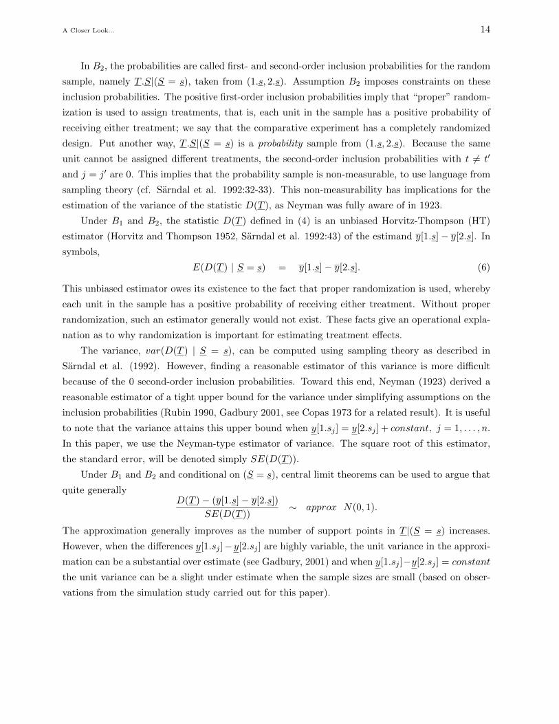
In B2, the probabilities are called first- and second-order inclusion probabilities for the random

sample, namely T .S|(S = s), taken from (1.s, 2.s). Assumption B2 imposes constraints on these

inclusion probabilities. The positive first-order inclusion probabilities imply that “proper” random-

ization is used to assign treatments, that is, each unit in the sample has a positive probability of

receiving either treatment; we say that the comparative experiment has a completely randomized

design. Put another way, T .S|(S = s) is a probability sample from (1.s, 2.s). Because the same

unit cannot be assigned different treatments, the second-order inclusion probabilities with t 6= t′

and j = j′ are 0. This implies that the probability sample is non-measurable, to use language from

sampling theory (cf. Sarndal et al. 1992:32-33). This non-measurability has implications for the

estimation of the variance of the statistic D(T ), as Neyman was fully aware of in 1923.

Under B1 and B2, the statistic D(T ) defined in (4) is an unbiased Horvitz-Thompson (HT)

estimator (Horvitz and Thompson 1952, Sarndal et al. 1992:43) of the estimand y[1.s]− y[2.s]. In

symbols,

E(D(T ) | S = s) = y[1.s]− y[2.s]. (6)

This unbiased estimator owes its existence to the fact that proper randomization is used, whereby

each unit in the sample has a positive probability of receiving either treatment. Without proper

randomization, such an estimator generally would not exist. These facts give an operational expla-

nation as to why randomization is important for estimating treatment effects.

The variance, var(D(T ) | S = s), can be computed using sampling theory as described in

Sarndal et al. (1992). However, finding a reasonable estimator of this variance is more difficult

because of the 0 second-order inclusion probabilities. Toward this end, Neyman (1923) derived a

reasonable estimator of a tight upper bound for the variance under simplifying assumptions on the

inclusion probabilities (Rubin 1990, Gadbury 2001, see Copas 1973 for a related result). It is useful

to note that the variance attains this upper bound when y[1.sj ] = y[2.sj ] + constant, j = 1, . . . , n.

In this paper, we use the Neyman-type estimator of variance. The square root of this estimator,

the standard error, will be denoted simply SE(D(T )).

Under B1 and B2 and conditional on (S = s), central limit theorems can be used to argue that

quite generallyD(T )− (y[1.s]− y[2.s])

SE(D(T ))∼ approx N(0, 1).

The approximation generally improves as the number of support points in T |(S = s) increases.

However, when the differences y[1.sj ]− y[2.sj ] are highly variable, the unit variance in the approxi-

mation can be a substantial over estimate (see Gadbury, 2001) and when y[1.sj ]−y[2.sj ] = constant

the unit variance can be a slight under estimate when the sample sizes are small (based on obser-

vations from the simulation study carried out for this paper).

A Closer Look... 15

8.1 Fisher-Type Randomization Test: What Would Fisher Do?

Fisher tacitly (Welch 1937, Rubin 1990, 2005) used the no-unit-specific-effects hypothesis in this

setting. That is, it can be presumed that to Fisher, the no-treatment-effect hypothesis had the

form:

HRU.s0 : y[1.sj ] = y[2.sj ], j = 1, . . . , n.

When H0 = (B1, B2, HRU.s0 ) holds, we have the following:

• E(D(T ) | S = s) = 0.

• The one-sided p-value

pval1D(t) = PH0(D(T ) ≥ D(t) | S = s) = PH0(T ∈ {t′ : D(t′) ≥ D(t)}|S = s)

is computable because D(t′) is computable for every t′. This follows because, under HRU.s0 ,

y[1.s, 2.s] is computable given the observed data y[t.s].

• pvalD(t) = PH0(|D(T )| ≥ |D(t)| | S = s) is a computable two-sided p-value.

• The test, reject H0 if and only if (pvalD(T ) ≤ α) is observed, has size ≤ α.

This test is called a Fisher-type randomization test because it is based on the randomization

approach and it was introduced by Fisher (1935).

If pvalD(t) ≤ α, we reject H0, but of course either H0 is true and a rare (probability ≤ α)

event has occurred or H0 is false. If we reject H0 but B1 and B2 are assumed to be true, then we

reject HRU.s0 ; that is, we have statistical evidence that for at least one unit sj , y[1.sj ] 6= y[2.sj ].

This Fisher-type randomization test based on D(T ) is tailored to detect differences between

y[1.s] and y[2.s]. To detect other differences, such as scale differences between the y[1.s] and y[2.s],

an alternative to D(T ) should be used.

Attractive features of this Fisher-type randomization test include the following: it has size

guaranteed to be no larger than α, it is valid when the sampling depends on the science (S 6⊥ Y );

it does not require a model for the science Y ; and it does not require an estimate of the variance,

var(D(T )|S = s).

Randomization vs. Permutation P-values: It is clear that this Fisher-type randomization test

is conceptually very different from the science-based permutation test. Indeed, as a rule, the

randomization p-value pvalD(t) is numerically different than the permutation conditional p-value

cpvalD(x). There is an exception to this rule. Consider the special case uniform randomization

distribution,

P (T = t′|S = s) =n1!n2!

n!1(t′ ∈ T ), (7)

where T is the set of all possible treatment assignments such that n1 units are assigned treat-

ment 1 and n2 are assigned treatment 2. In this case, cpvalD(x) = pvalD(t). It is this identity

that often leads practitioners to incorrectly conclude that the permutation test is identical to the

randomization test. See Ernst (2004) for an interesting discussion.

A Closer Look... 16

8.2 Neyman-Type Randomization Test: What Would Neyman Do?

Compared to Fisher, Neyman was apparently more interested in detecting non-zero treatment

effects of the aggregate variety, especially y[1.s] − y[2.s]. He apparently found it less practically

useful to detect unit-specific effects if the average effect was 0. For this reason, Neyman used the no-

average-effect hypothesis (cf. Welch 1937). That is, he viewed the no-treatment-effect hypothesis

as

HRA.s0 : y[1.s] = y[2.s].

Because HRA.s0 ⊃ HRU.s

0 , Neyman’s approach focused on a narrower set of alternatives than Fisher,

thereby opening up the possibility of finding a test with higher power than the Fisher-type ran-

domization test, at least for alternatives of practical (in Neyman’s view) interest.

When H0 = (B1, B2, HRA.s0 ) holds, we have the following:

• E(D(T ) | S = s) = 0.

• Conditional on (S = s), Z(T ) =D(T )

SE(D(T ))∼ approx N(0, 1).

• pval1Z(t) = PH0(Z(T ) ≥ Z(t) | S = s) ≈ P (N(0, 1) ≥ Z(t)) ≡ apval1Z(t). The approximate

p-value apval1Z(t) is called a Neyman-type randomization one-sided p-value.

• pvalZ(t) = PH0(|Z(T )| ≥ |Z(t)| | S = s) ≈ 2P (N(0, 1) ≥ |Z(t)|) ≡ apvalZ(t). The approxi-

mate p-value apvalZ(t) is a Neyman-type randomization two-sided p-value.

• The test, reject H0 if and only if (apvalZ(T ) ≤ α) is observed, has size ≈ α.

This test is called a Neyman-type randomization test because it is based on the randomization

approach and ideas in Neyman (1923).

If apvalZ(t) ≤ α, we reject H0, but of course either H0 is true and a rare (probability ≈ α)

event has occurred or H0 is false. If we reject H0 but B1 and B2 are assumed to be true, then we

reject HRA.s0 ; that is, we have statistical evidence that y[1.s] 6= y[2.s].

Why not use D(T ) rather than Z(T )? It is tempting to think that Neyman would approach

the testing problem in Fisher-like fashion and compute a p-value defined as

PH0(D(T ) ≥ D(t) | S = s) = PH0(T ∈ {t′ : D(t′) ≥ D(t)}).

However, Neyman would have recognized that the set {t′ : D(t′) ≥ D(t)}, and hence the p-value,

canNOT be computed under HRA.s0 . This computational problem stems from the fact that y[1.s, 2.s]

is only partially observed and, unlike under Fisher’s more restrictive HRU.s0 , is not determined by

y[t.s] under the no-average-effect hypothesis HRA.s0 . It follows that D(t′) cannot be computed for

any t′ not equal to the observed t. Hence, Fisher’s p-value approach is not available for testing

Neyman’s no-average-effect hypothesis.

Unlike the Fisher-type randomization test of HRU.s0 , the size of the Neyman test of HRA.s

0 is

not guaranteed to be less than or equal to α; it is only approximately size α. For smaller n1 and

n2 and when the more restrictive hypothesis HRU.s0 holds, the Neyman-type randomization test

A Closer Look... 17

tends to be anti-conservative, with size a bit larger than the nominal α. This follows because

the Neyman-type estimator of the variance tends to slightly under-estimate the true variance in

this case. For moderate n1 and n2 the approximation is usually reasonable provided D(T ) has

enough support points with respect to the T |(S = s) distribution. We empirically explore this

approximation below.

9 Selection-Based Inference

With the selection-based approach, we condition on the science (only (S, T ) is random) and use

y[t.s] ← Y [T .S] | (Y = y) ∼ y[T .S] | (Y = y)

to carry out inferences about y[1.P , 2.P ].

We will consider the candidate assumptions

C1 : (S, T ) ⊥ Y

C2 : The distribution of (S, T ) is completely known and satisfies...

P (T .S 3 t.i) > 0, i = 1, . . . , N, t = 1, 2.

P (T .S 3 t.i, T .S 3 t′.i′) > 0, unless t 6= t′ and i = i′.

In words, C1 implies that the selection is independent of the science. As discussed in the

science-based Section 7, this assumption is not usually tenable in practice because the sampling

and science are often dependent. This dependence typically stems from sampling on the basis of

covariates that are related to Y .

As discussed in the randomization-based section, assumption C2 imposes constraints on first-

and second-order inclusion probabilities. In this case, the random sample T .S is taken from

(1.P , 2.P ). The assumption implies that each of the 2N elements in (1.P , 2.P ) has a positive

probability of being selected. Thus, the random sample is a probability sample. The 0 second-

order inclusion probabilities implies that the probability sample is non-measurable.

Under C1 and C2, the statistic D(S, T ) defined in (5) is an unbiased Horvitz-Thompson (HT)

estimator (Horvitz and Thompson, 1952, Sarndal et al. 1992:43) of the estimand y[1.P ] − y[2.P ].

In symbols,

E(D(S, T )) = y[1.P ]− y[2.P ].

Just as with var(D(T )|S = s) in the randomization approach, the variance, var(D(S, T )), can be

computed and estimated using sampling theory. The variance estimation, however, is subject to the

same problems as in the randomization approach because of the non-measurability of probability

sample T .S. Suffice it to say that a reasonable Neyman-type estimator exists. Denote the square

root of this estimator by SE(D(S, T )).

Under C1 and C2, and using the same arguments as in the randomization approach, we have

that quite generally

D(S, T )− (y[1.P ]− y[2.P ])

SE(D(S, T ))∼ approx N(0, 1).

A Closer Look... 18

The approximation generally improves as the number of support points in T .S increases. However,

when the differences y[1.i]− y[2.i] are highly variable, the unit variance in the approximation can

be a substantial over estimate (see Gadbury, 2001).

9.1 Fisher-Type Selection Test: What Would Fisher Do?

It can be presumed that to Fisher, the no-treatment-effect hypothesis in this setting had the form:

HRU0 : y[1.i] = y[2.i], i = 1, . . . , N.

When H0 = (C1, C2, HRU0 ) holds, we have the following:

• E(D(S, T )) = 0.

• pval1D(s, t) = PH0(D(S, T ) ≥ D(s, t)) = PH0((S, T ) ∈ {(s′, t′) : D(s′, t′) ≥ D(s, t)}) is NOT

computable because D(s′, t′) is not computable for any s′ 6= s. This follows because for s′ 6= s,

there is an s′j such that both y[1.s′j ] and y[2.s′j ] are unobserved and hence not computable

even under HRU0 .

It follows that a Fisher-type selection test is not available in this selection-based setting. Fisher

would have to condition on the sample and be content using the randomization-based approach to

draw inferences about y[1.s, 2.s], rather than y[1.P , 2.P ].

9.2 Neyman-Type Selection Test: What Would Neyman Do?

In analogy to the randomization setting, Neyman would use the no-average-effect hypothesis:

HRA0 : y[1.P ] = y[2.P ].

When H0 = (C1, C2, HRA0 ) holds, we have the following:

• E(D(S, T )) = 0.

• Z(S, T ) =D(S, T )

SE(D(S, T ))∼ approx N(0, 1).

• pval1Z(s, t) = PH0(Z(S, T ) ≥ Z(s, t)) ≈ P (N(0, 1) ≥ Z(s, t)) ≡ apval1Z(s, t). The approxi-

mate p-value apval1Z(s, t) is called a Neyman-type selection one-sided p-value.

• pvalZ(s, t) = PH0(|Z(S, T )| ≥ |Z(s, t)|) ≈ 2P (N(0, 1) ≥ |Z(s, t)|) ≡ apvalZ(s, t)

The approximate p-value apvalZ(s, t) is a Neyman-type selection two-sided p-value.

• The test, Reject H0 if and only if (apvalZ(S, T ) ≤ α) is observed, has size ≈ α.

This test will be called a Neyman-type selection test because it is a selection-based approach that

is based on the ideas in Neyman (1923).

If apvalZ(s, t) ≤ α, we reject H0, but of course either H0 is true and a rare (probability ≈ α)

event has occurred or H0 is false. If we reject H0 but C1 and C2 are assumed to be true, then we

reject HRA0 ; that is, we have statistical evidence that y[1.P ] 6= y[2.P ].

Just as in the randomization setting, the size of the Neyman test of HRA0 is not guaranteed to

be less than or equal to α; it is only approximately size α. Remarks regarding the approximation

A Closer Look... 19

in this selection setting are analogous to those given at the end of Section 8.2, in the randomization

setting.

10 Empirical Investigations

10.1 Cell Phone Use Example (Revisited)

The science variable Y [t.i] is defined as the reaction time for the ith unit in population P when

exposed to treatment t. Inference about the science Y distribution will be difficult to describe

because the sample of 64 students was not taken from any well-defined population P . For any

substantively interesting population, for example, P = licensed drivers in Utah, the assumption

that S ⊥ Y is untenable given the haphazard nature of the sample selection. The untenability

of S ⊥ Y also implies that it will be difficult to carry out inferences about the population values

y[1.P , 2.P ] for any substantively interesting population P . For these reasons, it makes sense to

focus on inferences about the 128 potential values in y[1.s, 2.s]. That is, it is arguably better to

use randomization-based inference for this example.

We assume that the randomization was carried out mechanically so that T ⊥ Y |S and we

assume that the distribution of T |(S = s) is uniform in the sense of (7); that is, conditions B1

and B2 of Section 8 are assumed to hold. We will use the Fisher-type randomization test to test

the no-treatment-effect hypothesis HRU.s0 : y[1.sj ] = y[2.sj ], j = 1, . . . , 64 and the Neyman-type

randomization test to test the no-treatment-effect hypothesis HRA.s0 : y[1.s] = y[2.s].

For these data, we observe

D(t) = 51.59, Z(t) =51.59

19.30= 2.67, pvalD(t) = 0.0074, and apvalZ(t) = 0.0075.

Because the Fisher-type randomization p-value pvalD(t) = 0.0074 is small, we have sufficient

evidence to reject HRU.s0 ; there is statistical evidence that y[1.sj ] 6= y[2.sj ] for at least one subject

in the sample of 64. Because the Neyman-type randomization p-value apvalZ(t) = 0.0075 is small,

we have sufficient evidence to reject HRA.s0 ; there is statistical evidence that y[1.s] 6= y[2.s]. In

fact, because D(t) = 51.59 is a Horvitz-Thompson unbiased estimate of y[1.s]− y[2.s], see (6), the

Neyman test gives statistical evidence that the reaction time values are higher on average when

cell phones are used, at least for this sample of 64. In other words, there is statistical evidence of

a treatment effect.

For completeness and for comparison purposes, we also give the values of the other commonly

used p-values, viz., permutation, Wilcoxon, t(Welch), and t(pooled):

cpvalD(x) = 0.0074, pvalW (x) = 0.0184, apvalT (x) = 0.0110, and pvalTp(x) = 0.0107,

Strictly speaking, these are only applicable for science-based inference, so they are of questionable

utility for this example. As noted above, because the randomization distribution is uniform, the

permutation p-value cpvalD(x) is numerically (but not conceptually!) identical to the Fisher-type

randomization p-value pvalD(t).

A Closer Look... 20

All computations were carried out in R. The author has written code to compute the Neyman-

type randomization p-value. The Fisher-type randomization and permutation p-values were ap-

proximated using Monte-Carlo estimation (here we used 106 simulations) as carried out in

twot.permutation {DAAG}. The Wilcoxon p-value was computed using wilcox.test {stats}.Note that when there are ties, as there are in this example, wilcox.test only reports approximate

p-values.

10.2 A Small-Scale Simulation Study

This section empirically compares the operating characteristics of the different tests considered in

this paper, under a variety of scenarios. All computations were carried out in R, with p-values

computed as described at the end of the previous sub-section. The simulated data are generated

according to models of the form:

y[1.i] ← Y [1.i] IID ∼ [scenario],y[2.i] ← Y [2.i] ∼ [scenario], i = 1, . . . , Ns ← S|(Y = y) ∼ P (S = P | Y = y) = 1

t ← T |(Y = y, S = s) ∼ P (T = t′|Y = y, S = s) =n1!n2!

n!1(t′ ∈ T )

(8)

where T is the set of all possible treatment assignments such that n1 units receive treatment 1 and

n2 receive treatment 2. Looking back at the science-based assumptions of Section 7, we see that

A1 holds, but none of A2–A7 are guaranteed to hold. Both the randomization-based assumptions

B1 and B2 of Section 8 hold, as do both the selection-based assumptions C1 and C2 of Section 9. A

more extensive simulation would also investigate scenarios where more of the assumptions do not

hold.

For data-generation models of the form (8), we have that (i) the randomization- and selection-

based approaches are identical because the sample S is taken to be equal to the population P ,

which also implies that n = N ; and (ii) the permutation and Fisher-type randomization p-values

are numerically (not conceptually!) identical because the randomization distribution is uniform

over the set of all possible treatment assignments.

Although the permutation-, Wilcoxon-, and t-tests are science-based approaches, we will es-

timate their operating characteristics for both the science and randomization (here, randomiza-

tion=selection) distributions. Similarly, the Fisher- and Neyman-type randomization tests are

randomization-based approaches, but we report their operating characteristics for both the science

and the randomization distributions. In the tables below, the rows labeled “Randomization” give

Monte Carlo estimates of the power of the tests over the distribution T |(Y = y, S = s). The

rows labeled “Science” give Monte Carlo estimates of the power of the tests over the distribution

Y |(S = s, T = t). In all cases, the nominal size is set at α = 0.05.

Tables 3 - 6 about here.

The simulation results in Tables 3–6 give us a glimpse at the operating characteristics of the

A Closer Look... 21

tests for a variety of scenarios, labeled “Sc.#.” The following summary focuses on comparisons

between the Fisher- and Neyman-type randomization tests, but the table entries afford broader

comparisons.

For small n1, n2, when y[1.sj ]− y[2.sj ] = constant, the Neyman-type randomization test tends

to be just a bit anti-conservative for testing HRA.s0 ; that is, the actual size appears to be a little

larger than the nominal size (see scenarios 1, 2, and 6 of Table 3). This anti-conservativeness

presumably stems from the fact that the Neyman-type estimator of the variance, var(D(T )|S = s),

tends to be slightly biased on the low side when y[1.sj ]− y[2.sj ] = constant. For larger n1, n2, this

anti-conservativeness disappears (scenarios 1, 2, and 6 of Table 5).

When the differences y[1.sj ]− y[2.sj ] are highly variable, the Neyman-type randomization test

tends to be a bit conservative for testing HRA.s0 , although not as conservative as the Fisher-type

randomization test (scenarios 4 and 7 in Tables 3 and 5). This conservativeness presumably stems

from the fact that the Neyman-type estimator of the variance, var(D(T )|S = s), tends to be biased

on the high side when y[1.sj ]− y[2.sj ] are highly variable (see Gadbury 2001).

For small n1, n2, the Normal approximation to the Neyman-type test statistic can be unrea-

sonable when there are extreme outliers present (scenario 3 of Table 3). With larger n1, n2, the

Normal approximations become more reasonable in the presence of extreme outliers (scenario 3 of

Table 5).

In all of the simulation scenarios, the Neyman-type randomization test had higher power than

the Fisher-type randomization test (see Tables 4 and 6), especially when n1, n2 are smaller (see

Table 4). Of course, power comparisons are most useful when both tests have the same size.

Because neither of these tests has size exactly equal to the nominal 0.05, these power comparisons

should be considered carefully. In particular, in head-to-head comparisons, the Fisher test is at a

disadvantage because its actual size is guaranteed to be no larger than 0.05; the Neyman test has

size that is only approximately equal to, and can exceed, the nominal 0.05.

On the basis of this limited simulation study, we recommend that practitioners at least think

seriously about using the Neyman-type randomization test as an alternative to the Fisher-type

randomization test, especially when n1, n2 are moderate, say at least 10, and when there are no

extreme outliers.

11 Discussion

This paper used concepts from the rich literatures on causal analysis and finite-population sampling

theory to clear up some of the confusion that exists about tests of the no-treatment-effect hypoth-

esis in the comparative experiment setting. Our approach lends itself to explicit specifications of

the candidate no-treatment-effects hypotheses and targets of inference. We clearly distinguished

between three main inference approaches: science-based, randomization-based, and selection-based.

The commonly-used permutation test, Wilcoxon rank sum test, and two-sample t tests are examples

of science-based approaches. Examples of randomization-based approaches, include the commonly-

used Fisher-type randomization test and the less commonly-used Neyman-type randomization test.

A Closer Look... 22

We also described a Neyman-type selection test. A small-scale empirical comparison of these differ-

ent tests was carried out. On the basis of the simulation results, we recommend that practitioners

consider using the Neyman-type randomization test in certain scenarios.

In our description of the science-based approach, we focused on testing hypotheses about the

distribution of Y . More generally, the science-based approach can be used to both estimate, or

test hypotheses about, characteristics of the distribution of Y and predict/estimate the unobserved

values y[−t.s]. Here, y[−A] is the collection of all 2N components of y excluding those with

subscripts in the set A. A look back at the assumptions A1–A7 shows that we did not have to

specify a model for the joint distribution of Y to carry out a test of no treatment effect. We only

assumed independence across units and modeled the marginal distributions of Y [1.i] and Y [2.i]. In

contrast, the prediction of unobserved values generally requires a model for the joint distribution

of Y , equivalently, a model for (Y [t.s], Y [−t.s]), the “(Yobs, Ymis)” of Rubin (e.g. 2005). Rubin

advocates using a Bayesian approach to science-based prediction of y[−t.s].This paper restricted attention to inferences about one population or sample, under two scenar-

ios corresponding to two treatments. Owing to randomization, we were able to compare these two

treatment scenarios; for example, see equation (6). Comparing two populations of distinct units is

a qualitatively different inference problem. However, similar notations and model structures can

be used to study this problem as well. Interestingly, in this two population setting, Fisher-type

randomization tests, as described herein, are generally not applicable. In contrast, the other tests

described in this paper, including the Neyman-type selection test, are applicable.

The notation and model structure introduced in this paper can be directly applied in more

general settings where there are more than two treatments being compared. There are extensions

in other directions. For example, rather than testing hypotheses, the ideas introduced in this paper

could be used to derive useful confidence intervals. More work in this direction will be forthcoming.

In the binary response, comparative experiment setting, Fisher’s exact test for 2×2 tables (see

Agresti, 2002:91) is equivalent to the Fisher-type randomization test of HRU.s0 when T ⊥ Y |S and

T |(S = s) has a uniform distribution as in (7); recall that HRU.s0 states that the binary response

values satisfy y[1.sj ] = y[2.sj ], j = 1, . . . , n. Fisher’s exact test is also equivalent to the permutation

test of HEU0 when (S, T ) ⊥ Y and Y [t.i] indep ∼ bin(1, πt); here HEU

0 is equivalent to π1 = π2.

In fact, in the simulation (scenarios 6 and 7 of Tables 3 and 5, and scenario 6 of Tables 4 and 6),

because of the uniform randomization distribution, we were able to use the R code for Fisher’s

exact test, fisher.test {stat}, to compute the exact values of the Fisher-type randomization

and permutation p-values. On a related note, we point out that the Neyman-type randomization

test is also available for testing the no-treatment-effect hypothesis HRA.s0 : y[1.s] = y[2.s] in 2 × 2

tables. This paper’s simulation results suggest that when the randomization distribution is uniform

as in (7), this Neyman-type randomization test for 2 × 2 tables may be somewhat more powerful

than Fisher’s exact test.

A Closer Look... 23

12 References

Agresti, A. (2002). Categorical Data Analysis, 2nd edition, New York: John Wiley and Sons, Inc.

Agresti, A and Franklin, C. (2007). Statistics: The Art and Science of Learning from Data,Pearson/Prentice Hall: Upper Saddle River, New Jersey.

Copas, J.B. (1973). “Randomization Models for the Matched and Unmatched 2×2 Tables,”Biometrika, Vol. 60, No. 3, 467-476.

Cox, D.R. (1958). The Planning of Experiments, New York: John Wiley and Sons, Inc.

Ernst, Michael D. (2004). “Permutation Methods: A Basis for Exact Inference,” Statistical Science,Vol. 19, No. 4, 676-685

Fisher, R. A. (1935). The Design of Experiments, Edinburgh:Oliver Boyd.

Gadbury, G.L. (2001). “Randomization Inference and Bias of Standard Errors,” The AmericanStatistician, Vol. 55. No. 4., 310-313.

Greenland, S. (1991). “On the Logical Justification of Conditional Tests for Two-by-Two Contin-gency Tables,” The American Statistician, Vol. 45, No. 3, 248-251.

Greenland, S. (2000), “Causal Analysis in the Health Sciences,” J. Amer. Statist. Assoc., Vol. 95,No. 449, 286-289

Holland, P.W. (1986). “Statistics and Causal Inference,” J. Amer. Statist. Assoc., Vol. 81, No.396, 945-968.

Hollander, M. and Wolfe, D.A. (1973). Nonparametric Statistical Methods, New York: John Wileyand Sons.

Horvitz, D.G. and Thompson, D.J. (1952). “A Generalization of Sampling without Replacementfrom a Finite Universe”, J. Amer. Statist. Assoc., Vol. 47, 663-685.

Kempthorne, O. (1952). The Design and Analysis of Experiments, New York: John Wiley andSons.

Kempthorne, O. (1955). “The Randomization Theory of Experimental Inference,” J. Amer. Stat.Assoc., Vol. 50, No. 271, 946-967.

Lehmann (1994). “Jerzy Neyman, 1894-1981: A Biographical Memoir,” in Biographical Memoirs,Vol. 63, edited by Office of the Home Secretary, National Academy of Sciences, WashingtonD.C.: National Academies Press.

Neyman, J. (1923). “On the Application of Probability Theory to Agricultural Experiments. Essayon Principles. Section 9,” Roczniki Nauk Rolniczych Tom X [in Polish]; English translation ofexcerpts by D.M. Dabrowska and T.P. Speed (1990), Statistical Science, Vol. 5, No. 4, 463-472.

Neyman, J. (1934). “On the Two Different Aspects of the Representative Method: The Method ofStratified Sampling and the Method of Purposive Sampling (with discussion),” J. Roy. Statist.Soc., Vol. 97, No. 4, 558-625.

Neyman, J. with cooperation of K. Iwaskiewicz and St. Kolodziejczyk (1935). “Statistical Problemsin Agricultural Experimentation (with discussion),” Suppl. J. Roy. Statist. Soc., Vol. 2, No. 2,107-180.

Pitman, E.J.G. (1937). “Significance Tests which can be Applied to Samples from any Populations,”Suppl. J. Roy. Statist. Soc., Vol. 4, No. 1, 119-130.

A Closer Look... 24

Pitman, E.J.G. (1938). Significance Tests which can be Applied to Samples from any Populations.III. The Analysis of Variance Test,” Biometrika, Vol. 29, 322-335.

Rosenbaum, P.R. (retrieved 1/13/12). URL www-stat.wharton.upenn/∼rosenbap/downloadTalks.htm

Rubin, D.B. (1990). “[On the Application of Probability Theory to Agricultural Experiments.Essay on Principles. Section 9.] Comment: Neyman (1923) and Causal Inference in Experimentsand Observational Studies,” Statistical Science, Vol. 5, No. 4, 472-480.

Rubin, D.B. (2004). “Teaching Statistical Inference for Causal Effects in Experiments and Obser-vational Studies,” J. Educ. and Behav. Statist., Vol. 29, No. 3, 343-367.

Rubin, D.B. (2005). “Causal Inference Using Potential Outcomes: Design, Modeling, Decisions,”J. Amer. Statist. Assoc., Vol. 100, No. 469, 322-331.

Rubin, D.B. (2010). “Reflections Stimulated by the Comments of Shadish (2010) and West andThoemmes (2010),” Psychological Methods, Vol. 15, No. 1, 38-46. doi: 10.1037/a0018537

Sarndal, C.E., Swensson, B. and Wretman, J. (1992). Model Assisted Survey Sampling, New York:Springer.

Strayer, D.L. and Johnston, W.A. (2001). “Driven to Distraction: Dual-Task Studies of SimulatedDriving and Conversing on a Cellular Telephone,” Psychological Science, Vol. 12, No. 6, pp.462-466.

Welch, B.L. (1937). “On the z-Test in Randomized Blocks and Latin Squares,” Biometrika, Vol.29, No. 1/2, 21-52.

Welch, B.L. (1938). “The Significance of the Difference Between Two Means when the PopulationVariances are Unequal,” Biometrika, Vol. 29, No. 3/4, 350-62.

Wilcoxon F. (1945), “Individual Comparisons by Ranking Methods,” Biometrics Bulletin, Vol. 1,No. 6, 80-83.

A Closer Look... 25

Table 3. Monte Carlo Estimates of Power when n1 = n2 = 10, Nominal Size=5%.

n1=n2 = 10 Permutationa Wilcoxon t(Welch) t(Pooled) Fishera NeymanHU

0 y[1.i]← Y [1.i] IID ∼ N(10, 22)true y[2.i]← Y [2.i] = Y [1.i], i = 1, . . . , 20. Sc.1Randomization 4.6 3.6 4.7 4.7 4.6 6.5Science 4.3 3.4 4.2 4.3 4.3 6.9

HU0 y[1.i]← Y [1.i] IID ∼ Gamma(shape = 1, scale = 5)

true y[2.i]← Y [2.i] = Y [1.i], i = 1, . . . , 20. Sc.2Randomization 5.0 4.9 4.1 4.6 5.0 7.4Science 4.0 4.1 3.2 3.5 4.0 7.7

HU0 y[1.i]← Y [1.i] IID ∼ 0.9U(0, 20) + 0.1U(200, 201), “mixture of uniforms”

true y[2.i]← Y [2.i] = Y [1.i], i = 1, . . . , 20. Sc.3Randomizationb 4.6 3.9 0.0 0.0 4.6 0.0Science 3.8 3.5 1.1 1.8 3.8 11.2

HEU.10 , HRA.s

0 y[1.i]← Y [1.i] IID ∼ N(10, 22)

true y[2.i]← Y [2.i] = Y [1.i] + Ei − E, Ei IID ∼ N(0, 32), i = 1, . . . , 20. Sc.4Randomization 1.5 1.9 1.7 1.8 1.5 3.3Science 2.7 2.0 2.5 2.6 2.7 4.2

HEU.10 , HRA.s

0 y[1.i]← Y [1.i] IID ∼ Gamma(shape = 1, scale = 5)

true y[2.i]← Y [2.i] = 2Y [1.i]− Y [1.P ], i = 1, . . . , 20. Sc.5Randomization 4.8 6.8 4.3 4.4 4.8 7.6Science 4.0 7.4 3.6 3.7 4.0 7.4

HU0 y[1.i]← Y [1.i] IID ∼ bin(1, 0.28)

true y[2.i]← Y [2.i] = Y [1.i], i = 1, . . . , 20. Sc.6Randomizationc 0.0 NA 9.1 9.1 0.0 9.1Science 2.1 NA 4.5 4.5 2.1 11.3

HEU0 , HRA.s

0 y[1.i]← Y [1.i] IID ∼d bin(1, 0.28)true y[2.i]← Y [2.i] IID ∼d bin(1, 0.28), corr(Y [1.i], Y [2.i]) = 0.37, i = 1, . . . , 20. Sc.7Randomizatione 0.4 NAf 1.6 1.6 0.4 4.6Science 0.2 NA 1.0 1.0 0.2 3.7

Table entries give the percent of times out of 1000 the simulated data gave a p-value ≤ 5%.

All indented hypotheses are also true, see Section 4.2. For example, in row 1, HU0 is true. It follows that all

the other hypotheses in Section 4.2 are also true.

a For this simulation, the permutation and Fisher-type randomization test results are numerically identical.

b The fixed y includes one large observation from the U(200, 201) distribution.

c The fixed y[1.P ] = 0 0 0 0 0 1 0 0 0 0 0 0 0 0 0 1 1 0 1 0 = y[2.P ].

d This is an approximation because the Y values are adjusted to satisfy HRA.s0 .

e The fixed y[1.P ] =1 0 0 1 0 1 0 1 0 0 1 0 0 1 0 0 0 0 0 0, y[2.P ] = 0 0 0 0 1 1 0 1 0 0 1 0 0 1 1 0 0 0 0 0.

f Because of the many ties in the binomial case, the Wilcoxon test as described herein is not applicable.

A Closer Look... 26


n1=n2 = 10 Permutationa Wilcoxon t(Welch) t(Pooled) Fishera NeymanHEU.1

0 , HRA.s0 y[1.i]← Y [1.i] IID ∼ N(10, 22)

false y[2.i]← Y [2.i] = Y [1.i] + 2, i = 1, . . . , 20. Sc.1Randomization 52.7 49.3 51.3 52.5 52.7 59.9Science 55.9 51.6 55.5 56.1 55.9 62.7

HEU.10 , HRA.s

0 y[1.i]← Y [1.i] IID ∼ N(10, 22)

false y[2.i]← Y [2.i] = Y [1.i] + 2 + Ei − E, Ei IID ∼ N(0, 32), i = 1, . . . , 20. Sc.2Randomization 26.2 23.6 24.1 25.7 26.2 35.6Science 28.6 23.8 26.1 27.2 28.6 36.6

HEU.10 , HRA.s

0 y[1.i]← Y [1.i] IID ∼ N(10, 22)false y[2.i]← Y [2.i] = 1.2Y [1.i], i = 1, . . . , 20. Sc.3Randomization 34.7 27.1 34.8 35.3 34.7 43.0Science 48.4 43.0 47.5 48.4 48.4 57.2

HEU.10 , HRA.s

0 y[1.i]← Y [1.i] IID ∼ Gamma(shape = 1, scale = 5)false y[2.i]← Y [2.i] = 2Y [1.i], i = 1, . . . , 20. Sc.4Randomization 19.2 12.9 16.1 18.7 19.2 28.6Science 30.2 23.7 23.4 26.0 30.2 38.5

HEU.10 , HRA.s

0 y[1.i]← Y [1.i] IID ∼ Gamma(shape = 1, scale = 5)false y[2.i]← Y [2.i] = 3Y [1.i] + Ei, Ei IID ∼ N(0, 52), i = 1, . . . , 20. Sc.5Randomization 45.7 28.6 40.2 45.3 45.7 65.5Science 49.2 38.1 39.8 44.4 49.2 63.5

HEU.10 , HRA.s

0 y[1.i]← Y [1.i] IID ∼ bin(1, 0.28)false y[2.i]← Y [2.i] IID ∼ bin(1, 0.71), corr(Y [1.i], Y [2.i]) = 0.29, i = 1, . . . , 20. Sc.6Randomizationb 18.9 NA 37.3 37.3 18.9 37.4Science 29.6 NA 48.0 48.0 29.6 50.3



b The fixed y[1.P ] = 0 0 0 0 0 1 0 0 1 0 1 0 0 0 0 1 1 0 1 0, y[2.P ] = 0 1 1 1 1 1 1 0 1 0 1 1 0 0 1 1 1 0 1 1.

A Closer Look... 27


n1=n2 = 50 Permutationa Wilcoxon t(Welch) t(Pooled) Fishera NeymanHU

0 y[1.i]← Y [1.i] IID ∼ N(10, 22)true y[2.i]← Y [2.i] = Y [1.i], i = 1, . . . , 100. Sc.1Randomization 4.0 4.0 4.0 4.0 4.0 4.4Science 4.7 4.8 4.8 4.8 4.7 5.5

HU0 y[1.i]← Y [1.i] IID ∼ Gamma(shape = 1, scale = 5)

true y[2.i]← Y [2.i] = Y [1.i], i = 1, . . . , 100. Sc.2Randomization 4.9 5.0 4.8 4.8 4.9 5.4Science 4.1 3.9 3.9 3.9 4.1 4.8

HU0 y[1.i]← Y [1.i] IID ∼ 0.9U(0, 20) + 0.1U(200, 201), “mixture of uniforms”

true y[2.i]← Y [2.i] = Y [1.i], i = 1, . . . , 100. Sc.3Randomizationb 4.2 6.5 4.3 4.5 4.2 8.6Science 5.3 5.4 5.3 5.3 5.3 6.6

HEU.10 , HRA.s

0 y[1.i]← Y [1.i] IID ∼ N(10, 22)

true y[2.i]← Y [2.i] = Y [1.i] + Ei − E, Ei IID ∼ N(0, 32), i = 1, . . . , 100. Sc.4Randomization 2.5 3.1 2.4 2.4 2.5 3.4Science 3.0 4.6 2.9 3.2 3.0 3.9

HUE.10 , HRA.s

0 y[1.i]← Y [1.i] IID ∼ Gamma(shape = 1, scale = 5)

true y[2.i]← Y [2.i] = 2Y [1.i]− Y [1, P ], i = 1, . . . , 100. Sc.5Randomization 4.6 42.5 4.4 4.4 4.6 6.1Science 2.8 35.1 2.8 2.8 2.8 5.0

HU0 y[1.i]← Y [1.i] IID ∼ bin(1, 0.28)

true y[2.i]← Y [2.i] = Y [1.i], i = 1, . . . , 100. Sc.6Randomizationc 2.2 NA 5.5 5.5 2.2 5.5Science 3.5 NA 5.0 5.0 3.5 5.9

HEU0 , HRA.s

0 y[1.i]← Y [1.i] IID ∼d bin(1, 0.28)true y[2.i]← Y [2.i] IID ∼d bin(1, 0.28), corr(Y [1.i], Y [2.i]) = 0.37, i = 1, . . . , 100. Sc.7Randomizatione 0.5 NA 0.8 0.8 0.5 1.0Science 1.6 NA 2.8 2.8 1.6 3.5



b The fixed y includes 7 large observations from the U(200, 201) distribution.

c The fixed y[1.P ] = y[2.P ] with y[1.P ] = y[2.P ] = 32/100.

d This is an approximation because the Y values are adjusted to satisfy HRA.s0 .

e The fixed y is such that y[1.P ] 6= y[2.P ], y[1.P ] = y[2.P ] = 33/100, and corr(y[1.P ], y[2.P ]) = 0.186.

A Closer Look... 28


n1=n2 = 50 Permutationa Wilcoxon t(Welch) t(Pooled) Fishera NeymanHEU.1

0 , HRA.s0 y[1.i]← Y [1.i] IID ∼ N(10, 22)

false y[2.i]← Y [2.i] = Y [1.i] + 1, i = 1, . . . , 100. Sc.1Randomization 80.9 76.4 80.4 80.4 80.9 81.3Science 69.5 67.7 69.9 69.9 69.5 70.4

HEU.10 , HRA.s

0 y[1.i]← Y [1.i] IID ∼ N(10, 22)

false y[2.i]← Y [2.i] = Y [1.i] + 1 + Ei − E, Ei IID ∼ N(0, 32), i = 1, . . . , 100. Sc.2Randomization 36.3 31.4 36.2 36.4 36.3 42.7Science 37.9 36.3 37.5 38.0 37.9 42.8

HEU.10 , HRA.s

0 y[1.i]← Y [1.i] IID ∼ N(10, 22)false y[2.i]← Y [2.i] = 1.1Y [1.i], i = 1, . . . , 100. Sc.3Randomization 70.5 68.6 71.0 71.1 70.5 72.1Science 66.6 63.9 65.7 65.7 66.6 67.4

HEU.10 , HRA.s

0 y[1.i]← Y [1.i] IID ∼ Gamma(shape = 1, scale = 5)false y[2.i]← Y [2.i] = 1.5Y [1.i], i = 1, . . . , 100. Sc.4Randomization 46.6 39.0 46.2 46.4 46.6 49.5Science 49.2 40.6 48.0 48.2 49.2 51.8

HEU.10 , HRA.s

0 y[1.i]← Y [1.i] IID ∼ Gamma(shape = 1, scale = 5)false y[2.i]← Y [2.i] = 1.5Y [1.i] + Ei, Ei IID ∼ N(0, 52), i = 1, . . . , 100. Sc.5Randomization 41.0 35.2 40.4 40.5 41.0 44.3Science 39.2 30.7 38.9 39.0 39.2 44.2

HEU.10 , HRA.s

0 y[1.i]← Y [1.i] IID ∼ bin(1, 0.28)false y[2.i]← Y [2.i] IID ∼ bin(1, 0.50), corr(Y [1.i], Y [2.i]) = 0.36, i = 1, . . . , 100. Sc.6Randomizationb 48.8 NA 58.8 58.8 48.8 60.3Science 51.1 NA 60.1 60.1 51.1 60.3



b The fixed y is such that y[1.P ] 6= y[2.P ], y[1.P ] = 24/100, y[2.P ] = 45/100, and corr(y[1.P ], y[2.P ]) =0.386.

no-treatment-e ect hypothesis in a comparative experiment1

Documents