nonlinear adaptative task space control for a 2-dof redundantly actuated parallel manipulator

Nonlinear Dyn (2010) 59: 61–72DOI 10.1007/s11071-009-9520-1

O R I G I NA L PA P E R

Nonlinear adaptive task space control for a 2-DOFredundantly actuated parallel manipulator

Weiwei Shang · Shuang Cong

Received: 21 February 2008 / Accepted: 27 April 2009 / Published online: 13 May 2009© Springer Science+Business Media B.V. 2009

Abstract A nonlinear adaptive (NA) controller in thetask space is developed for the trajectory tracking of a2-DOF redundantly actuated parallel manipulator. Thedynamic model with nonlinear friction is establishedin the task space for the parallel manipulator, andthe linear parameterization expression of the dynamicmodel is formulated. Based on the dynamic model, anew control law including adaptive dynamics compen-sation, adaptive friction compensation and error elim-ination items is designed. After defining a quadraticperformance index, the parameter update law is de-rived with the gradient descent algorithm. The stabil-ity of the parallel manipulator system is proved by theLyapunov theorem, and the convergence of the track-ing error and the error rate is proved by the Barbalat’slemma. The NA controller is implemented in the tra-jectory tracking experiments of an actual 2-DOF re-dundantly actuated parallel manipulator, and the ex-periment results are compared with the APD con-troller.

Keywords Parallel manipulator · Redundantactuation · Coulomb + viscous friction · Task space ·Nonlinear adaptive control

W. Shang · S. Cong (�)Department of Automation, University of Science andTechnology of China, Hefei, 230027, People’s Republicof Chinae-mail: [email protected]

1 Introduction

Over the past two decades, parallel manipulators haveattracted the attention of many researchers. Althougha vast literature is dedicated to kinematics and dy-namics, studies on control strategies are relativelyfew. In literature, there are two types of basic controlstrategies for parallel manipulators: kinematic controlstrategies and dynamic control strategies. In the kine-matic control strategies, parallel manipulators are de-coupled into a group of single-axis systems, so theycan be controlled by a group of individual controllers.Proportional-Derivative (PD) control [1, 2], nonlinearPD control [3, 4], and artificial-intelligence based con-trol [5, 6] belong to this type of control strategies.The nonlinear dynamics is not considered in thesecontrollers, so the complex computation of dynam-ics can be avoided and the controller design can besimplified considerably. However, these controllers donot always produce high performance, and there is noguarantee of stability at the high speed. Unlike thekinematic control strategies, full dynamic model ofparallel manipulator is taken into account in the dy-namic control strategies. So the nonlinear dynamicsof the manipulators can be compensated and higherperformance can be achieved with dynamic strategies.The traditional dynamic strategies are the augmentedPD (APD) controller and compute-torque controller[7, 8]. Furthermore, to gain a deep insight of the dy-namics and the traditional dynamic strategies of par-allel manipulators, Liu and Li [9] developed a unified

mailto:[email protected]

62 W. Shang, S. Cong

approach to model and control parallel manipulatorsbased on geometric projections, and Aghili [10] pro-posed a more generalized method to solve the dynamicproblem of parallel manipulators. Recently, some dy-namic controllers with performance indicators werepresented for parallel manipulators. Kim et al. [11]presented a robust nonlinear controller for the Stewartplatform. Vivas and Poignet [12] designed a predictivecontroller for a H4 parallel manipulator, and Shanget al. [13] developed an optimal controller for a 2-DOFredundantly actuated parallel manipulator. These dy-namic controllers can improve the performance of thetraditional dynamic controllers, but also require higheraccuracy of the dynamic models.

However, it is very difficult to get the accurate val-ues of the dynamic parameters of parallel manipula-tors. Therefore, designing adaptive controller for par-allel manipulators is very significant. The adaptivecontrollers have been used to control robotic manip-ulators extensively [14–16]. Yet, the studies on adap-tive control of parallel manipulators are relatively fewfor the complicated kinematics and dynamics. Walker[17] first presented a linear adaptive controller for aparallel manipulator. This method is based on a lin-earized model ignoring the highly coupled nonlineardynamics. Honegger et al. [18] developed a nonlinearadaptive (NA) controller for a 6-DOF parallel manip-ulator, but the computation amount is great for the in-verse matrix of the inertial matrix in the controller, andthe stability analysis of the controller is not shown.Strict mathematical proof on the stability of the NAcontroller for hydraulic parallel manipulator was givenby Sirouspour and Salcudean [19]. The above adap-tive controllers for parallel manipulators are designedin the joint space. Nevertheless, we are usually con-cerned about the trajectory tracking in the task space.Especially for the parallel manipulators with redun-dant actuators, the effect of the redundant actuators tothe end-effector motion can be fully considered in thetask space. Yiu and Li [20] developed adaptive controlin the task space for a 2-DOF redundantly actuatedparallel manipulator. Unfortunately, only simple vis-cous friction is considered in the dynamic model forthe controller design, which causes degradation of thecontrol performance in real system. Meanwhile, thecontroller design also lacks corresponding theoreticalanalysis of the stability.

In this paper, an NA controller is developed in thetask space for a 2-DOF redundantly actuated parallel

manipulator. The proposed controller includes adap-tive dynamics compensation, adaptive friction com-pensation and error elimination items. Based on theend-effector coordinate, the dynamic model of the par-allel manipulator is formulated in the task space. Inthe established model, the friction of three actuatedjoints is depicted with the Coulomb + viscous fric-tion model. For the nonlinearity and uncertainty ofthe dynamics and friction, the system dynamic andfriction parameters are estimated online by the gradi-ent descent algorithm. The performance index is com-posed of the trajectory tracking error and the error rate.Based on the APD controller, the adaptive control lawincluding adaptive dynamics compensation, adaptivefriction compensation and error elimination items isdesigned. The stability of the control system with theproposed NA controller is proved using the Lyapunovstability theorem. In addition to the theoretical devel-opment, the work here is validated using an actual 2-DOF redundantly actuated parallel manipulator. Thedetailed tuning procedures of the control parametersare given in the experiment. The experiment resultsshow that the proposed NA controller can get bettertrajectory tracking accuracy of the end-effector, com-paring with the APD controller.

The paper is organized as follows. In Sect. 2, thedynamic model of a 2-DOF redundantly actuated par-allel manipulator is established in the task space, andthe structural properties of the model are summarized.In Sect. 3, the dynamic and friction parameters areseparated from the dynamic model, and a linear pa-rameterization expression of the dynamic model is de-rived. In Sect. 4, the NA controller in the task space isdesigned, and the stability of the system and conver-gence of the tracking error and error rate are proved.In Sect. 5, the trajectory tracking experiments of anactual 2-DOF redundantly actuated parallel manipu-lator are implemented, and the experiment results arecompared with the APD controller. In Sect. 6, severalremarks are concluded.

2 Dynamic modeling

The experiment platform is a 2-DOF redundantlyactuated parallel manipulator. As shown in Fig. 1,a reference frame is established in the workspaceof the parallel manipulator. The unit of the frameis a meter. The parallel manipulator is actuated bythree servo motors located at the bases A1, A2,

Nonlinear adaptive task space control for a 2-DOF redundantly actuated parallel manipulator 63

Fig. 1 Coordinates of the 2-DOF redundantly actuated parallelmanipulator

and A3, and the end-effector is mounted at the com-mon joint O , where the three legs meet. Coordinatesof the three bases are A1 (0,0.25), A2 (0.433,0), andA3 (0.433,0.5), and all the links are of the same length0.244 m. The definitions of the joint angles are shownin Fig. 1, qa1, qa2, qa3 refer to the active joint anglesand qb1, qb2, qb3 refer to the passive joint angles.

In order to design the NA controller in the taskspace, the dynamic model in the task space should beformulated firstly. Cutting the parallel manipulator atthe common point O in Fig. 1, one can have an open-chain system including three independent 2-DOF ser-ial manipulators, each of which contains an active jointand a passive joint. The dynamic model of the paral-lel manipulator equals to the model of the open-chainsystem, plus the closed-loop constraints; thus the dy-namics of the parallel manipulator can be formulatedby combining the dynamics of the three serial manip-ulators under the constraints.

According to [21], the dynamic model of each2-DOF serial manipulator is given by

Miqi + Ciqi + fi = τi, (1)

where qi and qi are the joint acceleration and velocityrespectively, the subscript i denotes the ith serial ma-nipulator; Mi is the inertia matrix, and Ci is Coriolis

and centrifugal force matrix, which are defined as

Mi =[

αi γi cos(qai − qbi)

γi cos(qai − qbi) βi

],

Ci =[

0 γi sin(qai − qbi)qbi

−γi sin(qai − qbi)qai 0

],

where αi , βi , and γi are dynamic parameters. Theseparameters are related with the physical parameters,and are difficult to be measured accurately. Also, τi =[τai τbi]T is joint torque vector, where τai is the ac-tuated joint torque, the passive joint torque τbi = 0.fi = [fai fbi]T is the friction torque vector, where thepassive joint friction torque fbi can be ignored andonly the actuated joint friction torque fai is consid-ered. The actuated joint friction torque fai can be for-mulated as [22]

fai = sign(qai)fci + fvi qai , (2)

where fci represents the Coulomb friction, and fvi

represents the coefficient of the viscous friction.The dynamic model (1), which depicts the 2-DOF

serial manipulators, satisfies the following structuralproperties [21]:

(a) Mi is symmetric and positive.(b) Mi − 2Ci is skew-symmetric matrix.

After the dynamic models of three 2-DOF serialmanipulators are combined, the dynamic model of theopen-chain system can be expressed as

Mq + Cq + f = τ, (3)

where the symbols in (3) are defined as follows:

M =

⎡⎢⎢⎢⎢⎢⎢⎢⎢⎣

α1 0 0 γ1cab1 0 0

0 α2 0 0 γ2cab2 0

0 0 α3 0 0 γ3cab3

γ1cab1 0 0 β1 0 0

0 γ2cab2 0 0 β2 0

0 0 γ3cab3 0 0 β3

⎤⎥⎥⎥⎥⎥⎥⎥⎥⎦,

C =

⎡⎢⎢⎢⎢⎢⎢⎢⎢⎣

0 0 0 γ1sab1qb1 0 0

0 0 0 0 γ2sab2qb2 0

0 0 0 0 0 γ3sab3qb3

−γ1sab1qa1 0 0 0 0 0

0 −γ2sab2qa2 0 0 0 0

0 0 −γ3sab3qa3 0 0 0

⎤⎥⎥⎥⎥⎥⎥⎥⎥⎦

,


τ = [τa1, τa2, τa3, τb1, τb2, τb3]T,

f = [fa1, fa2, fa3, fb1, fb2, fb3]T,

q = [qa1 qa2 qa3 qb1 qb2 qb3 ]T,

where symbols cabi are defined as cabi =cos(qai − qbi), and symbols sabi are defined as sabi =sin(qai − qbi). So in the open-chain system modelequation (3), symbol M refers to the inertia matrix,C refers to the Coriolis and centrifugal force matrix,τ refers to the input torque vector, and f refers tothe friction torque vector. Note that the definition ofthe symbols is similar with these in serial manipula-tor dynamic model equation (1), only the difference isthat the symbols in (3) represent the whole open-chainsystem but not a 2-DOF serial manipulator. Thus,(3) also satisfies the similar structural properties as

follows:

(c) M is symmetric and positive.(d) M − 2C is skew-symmetric matrix.

Based on (3) of the open-chain system and the con-straint forces due to the closed-loop constraints, thedynamic model of the parallel manipulator in the jointspace can be expressed as

Mq + Cq = τ − f + ATλ, (4)

where ATλ represents the constraint force vector; herematrix A is the differential of the closed-loop con-strained equation and λ is a multiplier representingthe magnitude of the constraint forces. The closed-loop constraint equations of the parallel manipulatorare given by

H(q) =

⎡⎢⎢⎢⎣

xa1 + l cos(qa1) + l cos(qb1) − xa2 − l cos(qa2) − l cos(qb2)

ya1 + l sin(qa1) + l sin(qb1) − ya2 − l sin(qa2) − l sin(qb2)

xa1 + l cos(qa1) + l cos(qb1) − xa3 − l cos(qa3) − l cos(qb3)

ya1 + l sin(qa1) + l sin(qb1) − ya3 − l sin(qa3) − l sin(qb3)

⎤⎥⎥⎥⎦ = 0. (5)

Differentiating (5), we have dH(q)dt

= ∂H(q)∂q

q = A(q)q = 0. The constraint matrix A can be written as

A =

⎡⎢⎢⎢⎣

−l sin(qa1) l sin(qa2) 0 −l sin(qb1) l sin(qb2) 0

l cos(qa1) −l cos(qa2) 0 l cos(qb1) −l cos(qb2) 0

−l sin(qa1) 0 l sin(qa3) −l sin(qb1) 0 l sin(qb3)

l cos(qa1) 0 −l cos(qa3) l cos(qb1) 0 −l cos(qb3)

⎤⎥⎥⎥⎦ . (6)

The constraint force ATλ in (4) is an unknown termand is difficult to be measured directly. Fortunately, theconstraint force ATλ can be eliminated by the expres-sion of the null-space of matrix A. With the Jacobianmatrix W , on can get

q = Wqe, (7)

where q = [qa1 qa2 qa3 qb1 qb2 qb3]T represents thevelocity vector of all the joints; qe = [x y]T representsthe velocity vector of the end-effector; the Jacobianmatrix W can be defined as

W =

⎡⎢⎢⎢⎢⎢⎢⎢⎢⎣

r1 cos(qb1) r1 sin(qb1)



−r1 cos(qa1) −r1 sin(qa1)



⎤⎥⎥⎥⎥⎥⎥⎥⎥⎦

,

where ri = 1

l sin(qbi − qai).

Considering the constraint equation Aq = 0, one

can have AWqe = 0 with the Jacobian relation (7).


The velocity vector qe of the end-effector containsindependent generalized coordinates, so one can getAW = 0, or equivalently,WTAT = 0. With this result,the term of ATλ can be eliminated from (4), and thedynamic model in the joint space can be written as

WTMq + WTCq + WTf = WTτ + WTATλ = WTτ.

(8)

In order to study both dynamic control and trajectoryplanning of the parallel manipulator both in the taskspace, we will further formulate the dynamic model inthe task space on the basis of (8) in the joint space.Differentiating the Jacobian relation (7) yields

q = W qe + Wqe (9)

and substituting (7) and (9) into (8), the dynamicmodel in the task space can be expressed as

WTMWqe + WT(MW + CW)qe + WTf = WTτ.

(10)

If the friction torque of the passive joints is ne-glected, (8) can be further simplified. Let τa and fa

be the actuator and friction torque vectors of the threeactuated joints, respectively, then WTτ = STτa , andWTf = STfa . Here, S is the Jacobian matrix betweenthe velocity of the end-effector and three actuatedjoints, and S can be written as

S =⎡⎣




⎤⎦ .

Then, the dynamic model in the task space can be for-mulated as

WTMWqe + WT(MW + CW)qe + STfa = STτa.

(11)

The above equation can be briefly expressed as

Meqe + Ceqe + STfa = STτa, (12)

where Me = WTMW is the inertial matrix in the taskspace, and Ce = WT(MW + CW) is the Coriolis andcentrifugal force matrix in the task space.

The dynamic model equation (12) in the task spacealso satisfies the similar structural properties with thedynamic model of the open-chain system or a 2-DOFserial manipulator as follows [8]:

(e) Me is symmetric and positive.(f) Me − 2Ce is skew-symmetric matrix.

3 Linear parameterization expression of thedynamic model

In order to realize effective dynamics and frictioncompensation, the parameters in dynamic model equa-tion (12) must be known. However, it is very difficultto know the precise value of these parameters. On theone hand, the dynamic parameters αi,βi , and γi aredifficult to be measured when the parallel manipulatoris assembled, and these parameters may be affected bythe load. On the other hand, the friction in the move-ment of the parallel manipulator is complex and non-linear, and the friction characteristics are related withthe changes of the velocity. For the Coulomb + vis-cous friction model defined by (2), the model para-meters fvi and fci are not constant when the veloc-ity changes. Thus, the dynamic parameters and fric-tion parameters should be estimated on-line, then thedynamics and friction compensation can be calculatedand adaptive control of the parallel manipulator can beimplemented.

To implement adaptive control for the parallel ma-nipulator, the system parameters including dynamicparameters of αi , βi , and γi , and friction parameters offvi and fci need to be identified firstly. When the sys-tem parameters are separated from the dynamic modelequation (12), we get a linear parameterization expres-sion of the system parameters of the dynamic modelequation (12), as follows:

Meqe + Ceqe + STfa = Y(q, q, qe, qe)θ, (13)

where θ is a 15 × 1 vector of the system parameterswhich contains nine dynamic parameters of αi , βi ,and γi , and six friction parameters of fvi and fci , θ

can be defined as

θ = [α1 α2 α3 β1 β2 β3 γ1 γ2 γ3

fv1 fv2 fv3 fc1 fc2 fc3]T

Y(q, q, qe, qe) is a 2 × 15 regression matrix, whenthe system parameters are separated from the dynamicmodel equation (12), the elements of the regressionmatrix can be written as

Y(j,1) = W1j (W11x + W11x + W12y + W12y),


Y(j,2) = W2j (W21x + W21x + W22y + W22y),

Y (j,3) = W3j (W31x + W31x + W32y + W32y),

Y (j,4) = W4j (W41x + W42y + W41x + W42y),

Y (j,5) = W5j (W51x + W52y + W51x + W52y),

Y (j,6) = W6j (W61x + W62y + W61x + W62y),

Y (j,7) = [(W11W4j + W41W1j )x

+ (W12W4j + W42W1j )y]cab1

+ [(W11W4j + W41W1j )x

+ (W12W4j + W42W1j )y]cab1

+ (W41W1j qb1 − W11W4j qa1)x · sab1

+ (W42W1j qb1 − W12W4j qa1)y · sab1,

Y (j,8) = [(W21W5j + W51W2j )x

+ (W22W5j + W52W2j )y]cab2

+ [(W21W5j + W51W2j )x

+ (W22W5j + W52W2j )y]cab2


+ (W52W2j qb2 − W22W5j qa1)y · sab2,

Y (j,9) = [(W31W6j + W61W3j )x

+ (W32W6j + W62W3j )y]cab3

+ [(W31W6j + W61W3j )x

+ (W32W6j + W62W3j )y]cab3


+ (W62W3j qb3 − W32W6j qa1)y · sab3,

Y (j,10) = W1j qa1, Y (j,11) = W2j qa2,

Y (j,12) = W3j qa3, Y (j,13) = U1j ,

Y (j,14) = U2j , Y (j,15) = U5j ,

where Wmj (or Wmj ) represents the mth row and j tharrangement element of the Jacobian matrix W (or W ,derivative of the Jacobian matrix W ), m = 1, . . . ,6,j = 1,2, the coefficients Uij are related with the direc-tion of the joint velocity, determining by the followingrules:

Uij ={

Wij , qai ≥ 0,

−Wij , qai < 0.

The linear parameterization expression in (13) ofthe system parameters is the basis of the parameter

identification for designing the NA controller. On theother hand, the expressions of the elements of the re-gression matrix Y(q, q, qe, qe) will be used to calcu-late the regression matrix of the NA controller.

4 Nonlinear adaptive controller

In this section, we will design the NA controller basedon the dynamic model equation (12) in the task spacefor the parallel manipulator. The system parameterscan be estimated by using the gradient descent algo-rithm based on the linear parameterization expressionin (13). Then, the stability of the closed system andthe convergence of the tracking error and the errorrate will be proved by the Lyapunov stability theorem,and the diagram of the whole control system will beshown.

4.1 Controller design

Let qde (t) be the desired trajectory of the end-effector

in the task space, then the actual tracking error is com-puted as

e = qde − qe. (14)

Then, one can define the combined error vector s as

s = e + Qe, (15)

where Q is a symmetric positive definite matrix. In-deed, s ≡ 0 represents a group of linear differentialequations whose unique solution is e ≡ 0, given theinitial conditions qd

e (0) = qe(0). Thus the convergenceproblem of e and e can be reduced to that of keepingthe vector s at zero. With (15), s can be written as

s = e + Qe. (16)

The reference tracking velocity qre and acceleration qr

e

can be defined as

qre = qe + s = qd

e + Qe, (17)

qre = qe + s = qd

e + Qe. (18)

Based on the dynamic model equation (12), the controllaw is designed as

STτa = Meqre + Ceq

re + STfa + Kds, (19)


where Me and Ce are calculated with the estimated dy-namic parameters, fa is calculated with the estimatedfriction parameters, and Kd is a symmetric positivedefinite matrix.

Control law (19) can be separated into three parts:the first part is the dynamics compensation, which iswritten as τe1 = Meq

re + Ceq

re ; the second part is the

friction compensation, which is written as τe2 = STfa;the third part is the extern PD tracking loop, which isused to eliminate the tracking error, and is written asτe3 = Kds = Kde + KdQe. Thus, the control law (19)can be rewritten as

STτa = τe1 + τe2 + τe3. (20)

We note that STτa in control law (20) is the actuatortorque in the task space, but in fact, we need the actua-tor torque τa of the three actuated joints. In practice, asolution that has a minimum weighted Euclidean normis selected as actual control input. The actual controlinput vector of the three actuated joints can be writtenas

τa = (ST)+

(τe1 + τe2 + τe3), (21)

where (ST)+ = S(STS)−1 is the Moore pseudo-inverse of ST, satisfying ST(ST)+ = I . For this re-dundantly actuated parallel manipulator, the singular-ity is eliminated in the effective workspace. Thus, thepseudo-inverse matrix (ST)+ will not close to a singu-larity for this redundantly actuated parallel manipula-tor.

One can see that the control law (19) is determinedby the estimated system parameters in Me, Ce, fa , andthe constant matrix Kd . Next we will formulate how tocalculate the estimated system parameters.

With the linear parameterization expression in (13),the first three terms in control law (19) can be writtenas

Meqre + Ceq

re + STfa = Y

(q, q, qr

e , qre

)θ , (22)

where θ is the estimated parameter vector of θ . Next,we will use the gradient descent algorithm for comput-ing the estimated parameter vector θ to minimize theperformance index J which can be defined as

J (θ , t) = 1

2

∫ t

t0

sT(θ , t

)Kds

(θ , t

)dλ. (23)

Calculating the partial derivative around θ , one canhave

∂J

∂θ=

∫ t

t0

∂sT

∂θKds dλ. (24)

With the gradient descent algorithm, θ should changeaccording to the direction of the gradient descent. Letθ = θ − θ denote the error vector of parameter estima-tion, then θ can be calculated by

θ = −Γ∂J

∂θ= −Γ

∫ t

t0

∂sT

∂θKds dλ, (25)

where Γ is a symmetric positive definite matrix. Con-sider θ as a slow-changing parameter vector, then˙θ = ˙

θ , and differentiating (25) by the time yields

˙θ = −Γ

∂sT

∂θKds. (26)

With the control law (19) and the parameterization ex-pression (22), one can have

∂sT

∂θ= −Y T(

q, q, qre , q

re

)K−1

d . (27)

Thus, the parameter update law can be expressed as

˙θ = Γ Y T(

q, q, qre , q

re

)s. (28)

With the estimated parameters θ , the control law (19)can be rewritten as

STτa = Y(q, q, qr

e , qre

)θ + Kds. (29)

In the following, with the NA controller including thecontrol law (29) and the parameter update law (28),we will get global stability of the parallel manipula-tor system, then the tracking error e, the error rate e,and the estimated parameter θ are bounded. And theconvergence of e and e will be further proved. In or-der to prove this conclusion, we will show two lemmasfirstly [23].

Lemma 1 If a differentiable function f (t) is boundedand decreasing (f (t) ≤ 0), then it converges to a limit.

Lemma 2 (Barbalat) If a differentiable function f (t)

has a finite limit as t → ∞, and if f (t) is uniformlycontinuous, then f (t) → 0 as t → ∞.


Theorem With the NA controller including controllaw (29) and parameter update law (28), the paral-lel manipulator system is globally stable, and e → 0and e → 0 as t → ∞.

Proof Choosing the Lyapunov function candidate as

V (t) = 1

2sTMes + 1

2θTΓ −1θ , (30)

it can be shown that the derivative of V (t) along tra-jectories of the closed-loop system becomes

V (t) = 1

2sTMes + sTMes + θTΓ −1 ˙

θ. (31)

Considering the structural properties (f), thensT(Me − 2Ce)s = 0, one can get

V (t) = sT[(Meq

re + Ceq

re

) − (Meqe + Ceqe)]

+ θTΓ −1 ˙θ. (32)

With the dynamic model equation (8) and the controllaw (29), one can have

Meqe + Ceqe = Y(q, q, qr

e , qre

)θ + Kds − STfa. (33)

And considering the linear parameterization expres-sion (13), one can get

Meqre + Ceq

re = Y

(q, q, qr

e , qre

)θ − STfa. (34)

Substituting (33) and (34) into (32), one gets

V (t) = −sTKds − sTY θ + θTΓ −1 ˙θ. (35)

Considering the parameter update law (28) and ˙θ = ˙

θ ,

then −sTY θ + θTΓ˙θ = 0, and one gets

V (t) = −sTKds ≤ 0. (36)

Therefore, the system is globally stable, then vectors and vector θ are bounded. From the definitions of s

and θ , one knows that e, e, and θ are bounded. Next,we will strictly prove the convergence of e and e.

Now, since V (t) ≥ 0 and V (t) ≤ 0, V (t) is boundedand decreasing. With Lemma 1, V (t) converges to alimit. From the expression (30) of V (t), this impliesthat both s and θ are bounded. Furthermore, this inturn implies that qe , qe and θ are all bounded. Con-sidering that the closed-loop dynamic equation can bewritten as

Mes + (Ce + Kd)s = Y θ, (37)

since Me is uniform positive definite, then M−1e exists

and bounded. Thus, one can have

s = M−1e Y θ − M−1

e (Ce + Kd)s. (38)

So s is also bounded. Considering

V (t) = −sTKds − sTKds = −2sTKds (39)

since both s and s are bounded, V (t) is bounded. Thus,V (t) is uniformly continuous. With Lemma 2, whent → ∞, V (t) → 0, and this implies s → 0. So, e → 0and e → 0 as t → ∞. �

4.2 System control strategy diagram

The system control strategy diagram with the NA con-troller is shown in Fig. 2, from which one can see thatthe control strategy consists of three main parts. Thepane with dash is the NA controller, which containsparameter update law (28) and control law (29). Theparameter update law (28) is calculated by the com-bined error vector s, regression matrix Y , and rate ma-trix Γ . The control law includes the dynamics com-pensation τe1, the friction compensation τe2, and theerror elimination item τe3. The dot-and-dash pane isthe signal processing part, which is designed to calcu-late the position and velocity coordinates of the end-effector, passive joint angles, and angular velocity ofall the joints with the actuated joint angles. The dot-ted pane part is used to compute the three importantsignals, qr

e , qre and s, with the desired trajectory and

the signals from the signal processing part. The threeparts constitute the whole NA control strategy for theparallel manipulator control system.

5 Actual system experiments and results analysis

As shown in Fig. 3, the actual experiment platformis a 2-DOF redundantly actuated parallel manipula-tor designed and produced by Googol Tech. Ltd. inShenzhen, China. It is equipped with three permanentmagnet synchronous servo motors with harmonic geardrives. The actuated joint angles are measured with theabsolute optical-electrical encoders. We programmedthe NA controller with the Visual C++, and the algo-rithms run on a Pentium III CPU at 733 MHz. Thesampling rate of the real time system used for the con-trol is 2 m/s.


Fig. 2 Diagram of the nonlinear adaptive control scheme

Fig. 3 The prototype of the 2-DOF redundantly actuated paral-lel manipulator

The desired trajectory of the end-effector is astraight line in the task space, the starting point is(0.22, 0.29) and the ending point is (0.27, 0.24), thusthe motion distance is 0.0707 m. The profile of thedesired velocity is a S-type curve [24]. In our exper-iment, both the low-speed and high-speed motion aretested. For the low-speed motion, the max velocity is0.2 m/s, the max acceleration is 5 m/s2, and the jerkis 200 m/s3. For the high-speed motion, the max ve-locity is 0.5 m/s, the max acceleration is 10 m/s2, andthe jerk is 400 m/s3. In the NA control experiment,the nominal values of the dynamic parameters in θ areselected as the initial values, shown in Table 1. Then,

Table 1 Initial values of the dynamic parameters

Parameter Value Parameter Value Parameter Value

(kg m2) (kg m2) (kg m2)

α1 0.0932 β1 0.0381 γ1 0.0426

α2 0.0427 β2 0.0085 γ2 0.0111

α3 0.0427 β3 0.0085 γ3 0.0111

Table 2 Initial values of the friction parameters

Parameter Value Parameter Value

(Ns) (Nm)

fv1 2.9936 fc1 0.4976

fv2 2.7617 fc2 0.4570

fv3 2.8771 fc3 0.3006

with the known dynamic parameters, the values of thefriction parameters in θ can be identified by the leastsquares method [22, 25], shown in Table 2. The identi-fied results are used as the initial values of the frictionparameters in the NA controller.

Moreover, to demonstrate that the NA controllercan improve the tracking accuracy of the end-effector,experiments using the APD controller [8] also havebeen carried out for comparison. The APD controlleris chosen because it has nonlinear dynamics compen-sation and friction compensation. In the APD con-


troller, the control input vector of the three actuatedjoints can be calculated as

τa = S(STS

)−1

× (Meq

de + Ceq

de + STfa + Kpe + Kve

), (40)

where e = qde − qe is the position error of the end-

effector; Kp and Kv are both symmetric, positive def-inite matrices of constant gain each. In the APD con-troller (40), Me and Ce can be calculated with the val-ues of the dynamic parameters shown in Table 1. Andfa can be calculated with the values of the friction pa-rameters shown in Table 2.

In fact, some other control parameters in two con-trollers are needed to be tuned and determined bythe actual experiments. For the APD controller, onlytwo controller parameters are required to be tuned, theproportional gain matrix Kp and derivative gain ma-trix Kv . And, the traditional tuning method of the well-known PD controller can be used to tune the APD con-troller parameters. Thus, we can get suboptimal pa-rameter values which have the satisfied performancefor the actual parallel manipulator. For the proposedNA controller, only three parameters are required tobe tuned: parameter Q, gain Kd , and the parameterupdate rate matrix Γ . Also, the similar method can beused to tune the parameters Q and Kd .

The procedures of tuning parameters in APD are asfollows:

1. Let the value of Kv be zero, and increase the valueof Kp from zero until the system shows a little os-cillation to some extent.

2. Keep Kp value tuned well in the first stage, andincrease the value of Kv to further improve the dy-namic performance.

3. Regulate finely the above two values and maketradeoffs between Kp and Kv .

Using the above procedures, the APD controller para-meters are tuned as follows: Kp =diag(35000, 35000),Kv =diag(300,300).

The procedures of tuning parameters Q and Kd inNA controller are similar to the procedures of tuningparameters Kp and Kv in APD controller. The detailedprocedures of tuning parameters in NA are as follows:

1. Let the value of Kd be an identity matrix, and in-crease the value of Q from zero until the systemshows a little oscillation to some extent.

2. Increase the value of Kd , and at the same time, de-crease the value of the Q tuned in the first stage.One has to make tradeoffs between Q and Kd toget a good performance.

3. Γ represents the update rate of system parameters.First, set Γ = 0, which means the controller workswith the initial values of θ . Then, the system per-formance can be improved by increasing the valueof Γ . We do not stop regulating the value of Γ un-til the system performance becomes worse. A toolarge value of Γ means the change rate of the esti-mated parameters is larger than the change rate ofactual system parameters, which also worsens theperformance.

In the actual experiment, by our careful reg-ulation, we obtain Kd = diag(195,195), Q =diag(280,280), Γ = 10−4 × diag(5,5,5,5,5,5,5,

5,5,200,200,200,50,50,50).

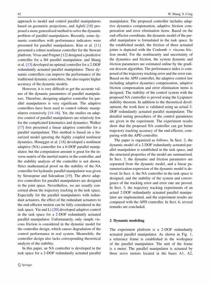
The experiment results of the low-speed motion areshown in Fig. 4. Figures 4(a) and (b), are the end-effector position errors of the x-direction (x-dir) andy-direction (y-dir), respectively. From the experimentcurves, one can see that the NA controller can de-crease the position errors of the x-dir and y-dir. Andin the acceleration process, the maximum position er-ror is much smaller with the NA controller. In the ac-tual experiment, we find that the NA controller canimprove the velocity tracking accuracy, in particular,restrain the impact from the acceleration and deceler-ation processes. In the actual experiment, we also findthat the estimated dynamic parameters have some fluc-tuations in the acceleration and deceleration processes.This implies that the nonlinear dynamic propertieshave obvious change in the acceleration and deceler-ation processes. The estimated viscous friction coeffi-cients are continuously fluctuant, while the Coulombfriction only contains small fluctuations. The fluctua-tions of the parameters are obvious, but insignificant.The fluctuations of the dynamic parameters and fric-tion parameters reflect the true change of the dynamicand friction properties.

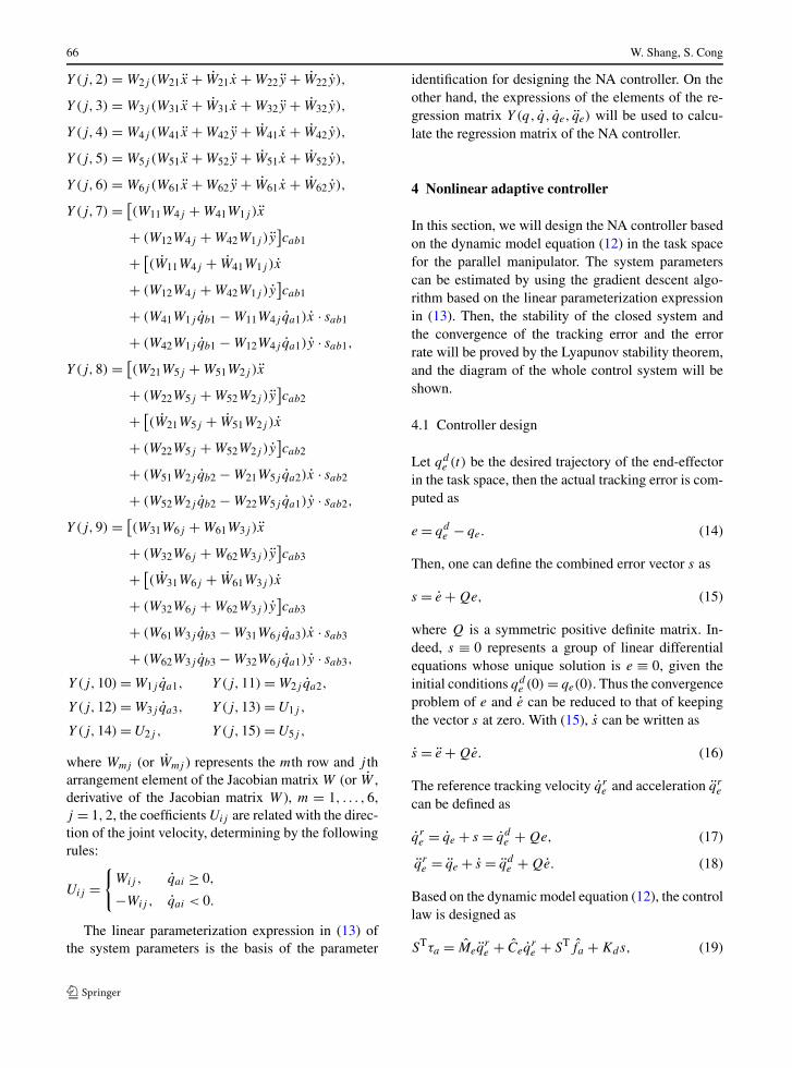
The experiment results at the high speed are shownin Fig. 5. Figures 5(a) and (b), are the end-effector po-sition errors of the x-dir and y-dir, respectively, fromwhich one can see obviously that the NA controllercan improve the position accuracy. The maximum po-sition error is smaller with the NA controller. In the ac-tual experiment, we also find the values change of theestimated dynamic parameters and friction parameters


(a)

(b)

Fig. 4 Position errors of the end-effector at the low-speed:(a) x-dir; (b) y-dir

at the high-speed motion are more obvious than thatat the low-speed motion. For the low-speed motion of0.2 m/s and the high-speed motion of 0.5 m/s, com-pared with the APD controller, the proposed NA con-troller can get a better position accuracy.

Furthermore, to evaluate the performances of twocontrollers, the root-square mean error (RSME) is se-lected as performance index. The RSME is defined asfollows:

RSME =√√√√ 1

N

N∑i=1

((xi − xi)2 + (yi − yi)2

), (41)

where xi , yi represent the position coordinates of theith point of the desired trajectory, and xi , yi representthe position coordinates of the ith point of the real tra-jectory.

The RSME of the trajectory tracking experiment atthe low- and high speed are shown in Table 3, in which

(a)

(b)

Fig. 5 Position errors of the end-effector at the high-speed:(a) x-dir; (b) y-dir

Table 3 RSME of the trajectory tracking experiments

Low-speed (m) High-speed (m)

APD 1.3738 × 10−4 4.7136 × 10−4

NA 8.4625×10−5 2.8299×10−4

RPE 38.40% 39.96%

the RPE is the reduced percentage of error. One cansee from Table 3 that the position accuracy increases38.40% at the low speed and 39.96% at the high speed,using the proposed NA controller, compared with theAPD controller.

6 Conclusion

An NA controller in the task space is proposed forthe trajectory tracking control of a parallel manipula-tor. The trajectory tracking experiments with the NA


controller are implemented for an actual 2-DOF re-dundantly actuated parallel manipulator. The NA con-troller proposed in this paper has the following ad-vantages: (1) Adaptive dynamics compensation canreduce the impact of nonlinear dynamics, in partic-ular the dramatic changes of the dynamics in accel-eration and deceleration processes. (2) Adaptive fric-tion compensation can achieve good friction compen-sation at both the low- and high-speed motion. (3) Er-ror elimination item can decrease the tracking errorand improve the tracking accuracy at the whole mo-tion process. In the NA controller design, the gradientdescent algorithm is used to estimate the system para-meters. The gradient descent algorithm is simple andeasy to implement in the actual experiment. However,the estimation efficiency may be further improved withother better algorithms.

Acknowledgements This work was supported in part bythe National Natural Science Foundation of China with GrantNo. 60774098, China Postdoctoral Science Foundation fundedproject with Grant No. 20080440717, and Anhui Provincial Nat-ural Science Foundation with Grant No. 090412040.

References

1. Wu, F.X., Zhang, W.J., Li, Q., Ouyang, P.R.: Integrateddesign and PD control of high-speed closed-loop mecha-nisms. J. Dyn. Syst. Meas. Control 124(4), 522–528 (2002)

2. Ghorbel, F.H., Chetelat, O., Gunawardana, R., Long-champ, R.: Modeling and set point control of closed-chainmechanisms: theory and experiment. IEEE Trans. ControlSyst. Technol. 8(5), 801–815 (2000)

3. Ouyang, P.R., Zhang, W.J., Wu, F.X.: Nonlinear PD con-trol for trajectory tracking with consideration of the designfor control methodology. In: Proc. IEEE Int. Conf. Robot.Autom., Washington, DC, May 2002, pp. 4126–4131

4. Su, Y.X., Duan, B.Y., Zheng, C.H., Zhang, Y.F., Chen,G.D., Mi, J.W.: Disturbance-rejection high-precision mo-tion control of a Stewart platform. IEEE Trans. ControlSyst. Technol. 12(3), 364–374 (2004)

5. Begon, P., Pierrot, F., Dauchez, P.: Fuzzy sliding mode con-trol of a fast robot. In: Proc. IEEE Int. Conf. Robot. Autom.,Nagoya, Japan, May 1995, pp. 1178–1183

6. Chung, I.F., Chang, H.H., Lin, C.T.: Fuzzy control of a six-degree motion platform with stability analysis. In: Proc.IEEE Int. Conf. Syst. Man. Cybern., Tokyo, Japan, Octo-ber 1999, pp. 325–330

7. Li, Q., Wu, F.X.: Control performance improvement of aparallel robot via the design for control approach. Mecha-tronics 14(8), 947–964 (2004)

8. Cheng, H., Yiu, Y.K., Li, Z.X.: Dynamics and control ofredundantly actuated parallel manipulators. IEEE Trans.Mechatronics 8(4), 483–491 (2003)

9. Liu, G.F., Li, Z.X.: A unified geometric approach to mod-eling and control of constrained mechanical systems. IEEETrans. Robot. Autom. 18(4), 574–587 (2002)

10. Aghili, F.: A unified approach for inverse and direct dy-namics of constrained multibody systems based on linearprojection operator: applications to control and simulation.IEEE Trans. Robot. Autom. 21(5), 834–849 (2005)

11. Kim, H.S., Cho, Y.M., Lee, K.I.: Robust nonlinear taskspace control for 6-DOF parallel manipulator. Automatica41, 1591–1600 (2005)

12. Vivas, A., Poignet, P.: Predictive functional control of a par-allel robot. Control Eng. Pract. 13, 863–874 (2005)

13. Shang, W.W., Cong, S., Zhang, Y.X.: Optimal control onparallel mechanism with planar 2-DOF redundant drives.J. Mach. Des. 23(8), 16–19 (2006)

14. Slotine, J.-J.E., Li, W.: Adaptive manipulator control:a case study. IEEE Trans. Autom. Control 33(11), 995–1003 (1988)

15. Sadegh, N., Horowitz, R.: An exponentially stable adaptivecontrol law for robot manipulators. IEEE Trans. Robot. Au-tom. 6(4), 491–496 (1990)

16. Feng, G., Palaniswami, M.: Adaptive control of robot ma-nipulator in task space. IEEE Trans. Robot. Autom. 38(1),100–104 (1993)

17. Walker, M.W.: Adaptive control of manipulator containingclosed kinematic loops. IEEE Trans. Robot. Autom. 6(1),10–19 (1990)

18. Honegger, M., Codourey, A., Burdet, E.: Adaptive controlof the Hexaglide, a 6-DOF parallel manipulator. In: Proc.IEEE Int. Conf. Robot. Autom., Albuquerque, NM, April1997, pp. 543–548

19. Sirouspour, M.R., Salcudean, S.E.: Nonlinear control of hy-draulic robots. IEEE Trans. Robot. Autom. 12(2), 173–182(2001)

20. Yiu, Y.K., Li, Z.X.: PID and adaptive robust control of a2-DOF over-actuated parallel manipulator for tracking dif-ferent trajectory. In: Proc. IEEE Int. Symp. Comp. Intell.Robot. Autom., Kobe, Japan, July 2003, pp. 1052–1057

21. Murray, R., Li, Z.X., Sastry, S.: A Mathematical Intro-duction to Robotic Manipulation. CRC Press, Boca Raton(1994)

22. Shang, W.W., Cong, S., Zhang, Y.X.: Nonlinear frictioncompensation of a 2-DOF planar parallel manipulator.Mechatronics 18(7), 340–346 (2008)

23. Slotine, J.-J.E., Li, W.P.: Applied Nonlinear Control. Pren-tice Hall, Englewood Cliffs (1991)

24. Shang, W.W., Cong, S.: Velocity planning algorithms ofparallel manipulator to improve control precision. J. Uni-versity Sci. Technol. China 36(8), 822–827 (2006)

25. Zhang, Y.X., Cong, S., Shang, W.W., Li, Z.X., Jiang, S.L.:Modeling, identification and control of a redundant planar2-DOF parallel manipulator. Int. J. Control Autom. Syst.5(5), 559–569 (2007)

nonlinear adaptative task space control for a 2-dof redundantly actuated parallel manipulator

Documents

dynamic control strategies

actuated parallel manipulator

parallel manipulator

hydraulic parallel manipulator

adaptive controller

nonlinearpd control

kinematic control strategies

dof parallel manipulator