Nonlinear Cyclic Truss Model for Beam-Column Joints of Non-ductile RC Frames

Jeremy Thomas Bowers

Thesis submitted to the faculty of the Virginia Polytechnic Institute and State University in

partial fulfillment of the requirements for the degree of

Master of Science

In

Civil Engineering

Ioannis Koutromanos, Chair

Finley A. Charney

Roberto T. Leon

6/24/14

Blacksburg, VA

Keywords: Reinforced Concrete, Beam-Column Joints, Seismic Analysis

Copyright

Nonlinear Cyclic Truss Model for Beam-Column Joints of Non-ductile RC Frames

Jeremy Thomas Bowers

ABSTRACT

Reinforced concrete (RC) moment frames comprise a significant portion of the built

environment in areas with seismic hazards. The beam-to-column joints of these frames are key

components that have a significant impact on the structure’s behavior. Modern detailing provides

sufficient strength within these joints to transfer the forces between the beams and the columns

during a seismic event, but existing structures built with poor detailing are still quite prevalent.

Identifying the need and extent of retrofits to ensure public safety through nondestructive means

is of primary importance. Existing models used to analyze the performance of RC beam-to-

column joints have either been developed for modern, well-detailed joints or are simplified so

that they do not capture a broad range of phenomena.

The present study is aimed to extend a modeling technique based on the nonlinear truss

analogy to the analysis of RC beam-to-column joints under cyclic loads. Steel and concrete

elements were arranged into a lattice truss structure with zero-length bond-slip springs

connecting them. A new steel model was implemented to more accurately capture the

constitutive behavior of reinforcing bars. The joint modeling approach captured well the shear

response of the joint. It also provided a good indication of the distribution of forces within the

joint.

The model was validated against three recently tested beam-column subassemblies.

These tests represented the detailing practice of poorly-detailed RC moment frames. The

analytical results were in good agreement with the experimental data in terms of initial stiffness,

strength and damage pattern through the joint.

iii

Acknowledgements

“Where there is no guidance, a people falls, but in an abundance of counselors there is safety.”

- Proverbs 11:14

I would like to thank those who have helped guide me in this process. To my fellow

student, Mohammadreza Gargari, I would like to show my appreciation for the advice and

assistance he gave along the way. I would also like to thank Professor Roberto Leon for the

impromptu meetings where he shared invaluable years of experience and Professor Finley

Charney for the counsel he gave. I must give a special thanks to my advisor, Professor Ioannis

Koutromanos, who spent countless hours teaching, counseling, and spurring me on to further

apply myself. Finally, I must give praise to God, through whose strength I have been able to

complete this work.

iv

Table of Contents

Chapter 1. Introduction .................................................................................................... 1

1.1 Background ........................................................................................................... 1

1.2 Thesis Scope .......................................................................................................... 4

1.3 Thesis Outline ....................................................................................................... 6

Chapter 2. Literature Review ........................................................................................... 8

2.1 Description of Joint Behavior ............................................................................... 8

2.2 Joint Models ........................................................................................................ 14

2.2.1 Empirical Joint Models .................................................................................. 14

2.2.2 Mechanistic Joint Models .............................................................................. 17

Chapter 3. Analysis Methodology .................................................................................. 24

3.1 Introduction ......................................................................................................... 24

3.2 Description of Nonlinear Truss Analogy for Beam-to-Column Joints ............... 24

3.2.1 Concrete Model .............................................................................................. 27

3.2.2 Transverse Strain Effect in Concrete ............................................................. 29

3.3 Enhancements to Truss Modeling Approach for Beam-to-Column Joints ......... 29

3.3.1 Effective Concrete Confinement Due to Axial Column Load ....................... 30

3.3.2 New Implementation of a Uniaxial Model for Steel Reinforcement ............. 31

3.3.3 Bond-Slip Model ............................................................................................ 36

Chapter 4. Validation of Analysis Methodology ........................................................... 39

v

4.1 Analysis of Interior Beam-to-Column Joints ...................................................... 39

4.1.1 Specimen Descriptions................................................................................... 40

4.1.2 Model Descriptions ........................................................................................ 43

4.1.3 .Discussion of Results .................................................................................... 47

4.2 Analysis of Exterior Beam-to-Column Joint ....................................................... 51

4.2.1 Specimen Description .................................................................................... 52

4.2.2 Model Description ......................................................................................... 54

4.2.3 Discussion of Results ..................................................................................... 56

4.3 Effects of Key Model Assumptions .................................................................... 58

Chapter 5. Conclusions and Recommendations for Future Research ............................ 61

5.1 Conclusions ......................................................................................................... 61

5.2 Recommendations for Future Research .............................................................. 62

References ......................................................................................................................... 63

Appendix A. DoddRestr Steel Constitutive Model Source Code ..................................... 66

vi

List of Figures

Figure 1.1 Partial collapse of Kaiser Permanente building during 1994 Northridge earthquake.

Hassan, W. M., Park, S., Lopez, R. R., Mosalam, K. M., and Moehle, J. P. (2010),

“Seismic Response of Older-Type Reinforced Concrete Corner Joints.” Proceedings of

the 9th U.S. National and 10th Canadian Conference on Earthquake Engineering,

Toronto, Ontario, Canada, Paper No. 1616. Photo used under fair use, 2014. ................... 3

Figure 1.2 Partial building collapse during 1999 Izmit earthquake. Sezen, H., Elwood, K. J.,

Whittaker, A. S., Mosalam, K. M., Walace, J. W., and Stanton, J. F., (2000), “Sezen -

Structural Engineering Reconnaissance of the August 17, 1999, Kocaeli (Izmit), Turkey,

Earthquake.” Report No. PEER-2000/09, Berkeley, CA. Photos used under fair use, 2014.

............................................................................................................................................. 3

Figure 1.3 Damage areas of the 1994 Northridge earthquake and the 1895 St. Louis earthquake.

Filson, J. R., McCarthy, J., Ellsworth, W. L., and Zoback, M. L. (2003), “The USGS

earthquake hazards program in NEHRP—Investing in a safer future.” USGS Fact Sheet

017-03, Reston, VA. Figure used under fair use, 2014....................................................... 4

Figure 1.4 Concrete spalling within beam-to-column joint core. Pantelides, C., Hansen, J.,

Nadauld, J., and Reaveley, L. (2002), “Assessment of Reinforced Concrete Building

Exterior Joints with Substandard Details.” Report No. PEER-2002/18, Berkeley, CA.

Photo used under fair use, 2014. ......................................................................................... 5

Figure 1.5 Connection types ........................................................................................................... 6

Figure 2.1 Joint shear transfer mechanisms. Leon, R. (1990), “Shear Strength and Hysteretic

Behavior of Interior Beam-Column Joints.” ACI Structural Journal 87(1), 3-11. Figures

used under fair use, 2014. ................................................................................................... 8

vii

Figure 2.2 Shear stress-strain points. Kim, J., and LaFave, J. (2006), "Key influence parameters

for the joint shear behaviour of reinforced concrete (RC) beam-column connections."

Engineering Structures 29, 2523-2539. Figure used under fair use, 2014. ...................... 13

Figure 2.3 Formation of joint shear cracks. Pantelides, C., Hansen, J., Nadauld, J., and Reaveley,

L. (2002), “Assessment of Reinforced Concrete Building Exterior Joints with

Substandard Details.” Report No. PEER-2002/18, Berkeley, CA. Photo used under fair

use, 2014. .......................................................................................................................... 13

Figure 2.4 Crushing within joint core. Pagni, C., and Lowes, L. (2004), “Predicting Earthquake

Damage in Older Reinforced Concrete Beam-Column Joints.” Report No. PEER-

2003/17, Berkeley, CA. Photo used under fair use, 2014. ................................................ 13

Figure 2.5 Joint shear stress vs. concrete compressive strength. Kim, J., and LaFave, J. (2006),

"Key influence parameters for the joint shear behaviour of reinforced concrete (RC)

beam-column connections." Engineering Structures 29, 2523-2539. Figure used under

fair use, 2014. .................................................................................................................... 13

Figure 2.6 Scissor model............................................................................................................... 15

Figure 2.7 Joint model by Biddah and Ghobarah (1999).............................................................. 16

Figure 2.8 Joint model by Birely et al. (2011) ............................................................................. 16

Figure 2.9 Joint model by Filippou et al. (1983) ......................................................................... 17

Figure 2.10 General model used by Lowes, Altoontash, and Mitra ............................................. 17

Figure 2.11 Lowes and Altoontash (2003) bond-slip envelope curve .......................................... 18

Figure 2.12 Verification of bond-slip model. Lowes, L., Mitra, N., and Altoontash, A. (2004), “A

Beam-Column Joint Model for Simulating the Earthquake Response of Reinforced

viii

Concrete Frames.” Report No. PEER-2003/10, Berkeley, CA. Figures used under fair

use, 2014. .......................................................................................................................... 18

Figure 2.13 Joint model by Shin and LaFave (2004)................................................................... 20

Figure 2.14 Diagonal struts of mechanistic joint model by Park and Mosalam (2009) ............... 21

Figure 2.15 Joint model by Sharma et al. (2011) .......................................................................... 21

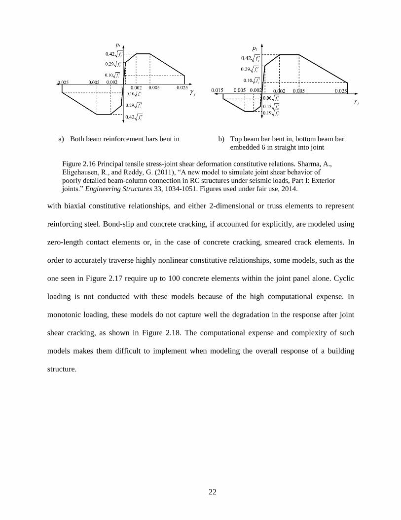
Figure 2.16 Principal tensile stress-joint shear deformation constitutive relations. Sharma, A.,

Eligehausen, R., and Reddy, G. (2011), “A new model to simulate joint shear behavior of

poorly detailed beam-column connection in RC structures under seismic loads, Part I:

Exterior joints.” Engineering Structures 33, 1034-1051. Figures used under fair use,

2014................................................................................................................................... 22

Figure 2.17 Finite element model. Pantazopoulou, S. J., and Bonacci, J. F. (1994), “On

earthquake-resistant reinforced concrete frame connections.” Canadian Journal of Civil

Engineering 21, 307-328. Figure used under fair use, 2014. ............................................ 23

Figure 2.18 Load-deflection response of finite element joint model compared with measured

response. Baglin, R. H., and Scott, P. S. (2000), “Finite Element Modeling of Reinforced

Concrete Beam-Column Connections.” ACI Structural Journal 97(6), 886-894. Figure

used under fair use, 2014. ................................................................................................. 23

Figure 3.1 Proposed model layout ................................................................................................ 26

Figure 3.2 Lu and Panagiotou (2013) uniaxial stress-strain law for concrete .............................. 27

Figure 3.3 Transverse strain strength reduction factor ................................................................. 29

Figure 3.4 Concrete confinement pressure ................................................................................... 30

Figure 3.5 Dodd and Restrepo-Posada (1995) constitutive law for steel ..................................... 32

Figure 3.6 Loading reversals......................................................................................................... 34

ix

Figure 3.7 Measured and simulated cyclic stress-strain response of steel model ......................... 36

Figure 3.8 Bond-slip model by Mitra and Lowes (2007) ............................................................. 38

Figure 4.1 Reinforcement detailing of interior beam-column assemblies. Alire, D. (2002),

“Seismic Evaluation of Existing Unconfined Reinforced Concrete Beam-Column Joints.”

M.S. Thesis, University of Washington, Seattle, WA, 306pp. Figures used under fair use,

2014................................................................................................................................... 40

Figure 4.2 Comparison of experimental data to Dodd-Restrepo steel constitutive model ........... 42

Figure 4.3 Applied drift history for the specimens tested by Alire (2002) ................................... 42

Figure 4.4 Interior joint model layout ........................................................................................... 44

Figure 4.5 Types of shear strain .................................................................................................... 46

Figure 4.6 Measurement of shear strain. Alire, D. (2002), “Seismic Evaluation of Existing

Unconfined Reinforced Concrete Beam-Column Joints.” M.S. Thesis, University of

Washington, Seattle, WA, 306pp. Figures used under fair use, 2014. ............................. 46

Figure 4.7 Description of joint shear stress parameters ................................................................ 46

Figure 4.8 Column shear force-drift responses for the first inter joint ......................................... 47

Figure 4.9 Observed concrete spalling at 3% drift. Alire, D. (2002), “Seismic Evaluation of

Existing Unconfined Reinforced Concrete Beam-Column Joints.” M.S. Thesis, University

of Washington, Seattle, WA, 306pp. Photo used under fair use, 2014. ............................ 48

Figure 4.10 Simulated concrete crushing during 3% drift load level ........................................... 48

Figure 4.11 Joint shear stress-joint shear strain responses for the first interior joint. .................. 49

Figure 4.12 Column shear force-drift responses for the second interior joint. ............................. 50

x

Figure 4.13 Crack patterns of second interior joint. Alire, D. (2002), “Seismic Evaluation of

Existing Unconfined Reinforced Concrete Beam-Column Joints.” M.S. Thesis, University

of Washington, Seattle, WA, 306pp. Figures used under fair use, 2014. ......................... 50

Figure 4.14 Joint shear stress-joint shear strain responses for the second interior joint ............... 51

Figure 4.15 Reinforcement detailing of the exterior joint. Pantelides, C., Hansen, J., Nadauld, J.,

and Reaveley, L. (2002), “Assessment of Reinforced Concrete Building Exterior Joints

with Substandard Details.” Report No. PEER-2002/18, Berkeley, CA. Figure used under

fair use, 2014. .................................................................................................................... 53

Figure 4.16 Applied drift history for the specimen tested by Pantelides et al. (2002) ................. 54

Figure 4.17 Exterior joint model layout ........................................................................................ 55

Figure 4.18 Lateral load-drift responses for the exterior joint ...................................................... 57

Figure 4.19 Observed cracking pattern at formation of joint shear mechanism. Pantelides, C.,

Hansen, J., Nadauld, J., and Reaveley, L. (2002), “Assessment of Reinforced Concrete

Building Exterior Joints with Substandard Details.” Report No. PEER-2002/18, Berkeley,

CA. Photo used under fair use, 2014. ............................................................................... 57

Figure 4.20 Simulated crack pattern at first concrete crushing .................................................... 57

Figure 4.21 Normalized joint shear stress-joint shear strain responses for the exterior joint ....... 58

Figure 4.22 Comparison of experimental lateral load-drift response to simulated lateral load-drift

responses with and without bond-slip effect ..................................................................... 59

Figure 4.23 Comparison of experimental lateral load-drift response to simulated lateral load-drift

responses with and without confinement effect ................................................................ 60

xi

List of Tables

Table 3.1 Calibrated Steel Material Properties for Steel Coupon ................................................. 36

Table 4.1 Alire Reinforcement Properties .................................................................................... 42

Table 4.2 Alire Displacement History .......................................................................................... 42

Table 4.3 Exterior Joint Reinforcement Properties....................................................................... 54

Table 4.4 Pantelides Displacement History .................................................................................. 54

1

Chapter 1. Introduction

1.1 Background

Reinforced concrete (RC) buildings comprise a significant portion of the built

environment in the United States due to their relatively low cost and flexibility in building form.

Lateral loads in RC buildings can be resisted by two types of lateral load resisting systems: shear

walls or moment frames. Moment frames are assemblies of beams and columns connected by

beam-to-column joints. This type of system leaves a greater amount of open floor space within

the building interior, which is much more attractive from an architectural point of view. This

system also relies heavily on the ability of the beam-to-column joint to transfer the moment due

to lateral loads between the columns and the beams. Brittle failure leading to a sudden, drastic

decrease in strength can be a dire consequence of insufficient loading capacity and ductility

within this joint. For this reason, more stringent requirements have been placed on the detailing

of beam-to-column joints since the mid-1970’s in order to ensure that the joint has adequate

strength and in case of yielding, can undergo a relatively large amount of deformation without a

complete loss of strength. These newer beam-to-column joint details are referred to as ductile,

whereas those resulting in poor system deformation capacity are referred to as nonductile.

Many current RC structures, especially older structures and structures built in areas with

less frequent seismic activity, still maintain nonductile detailing. The high vulnerability of RC

moment frame buildings with nonductile beam-to-column joints (nonductile RC frames) has

been made apparent during the relatively moderate recent earthquakes in Northridge, California,

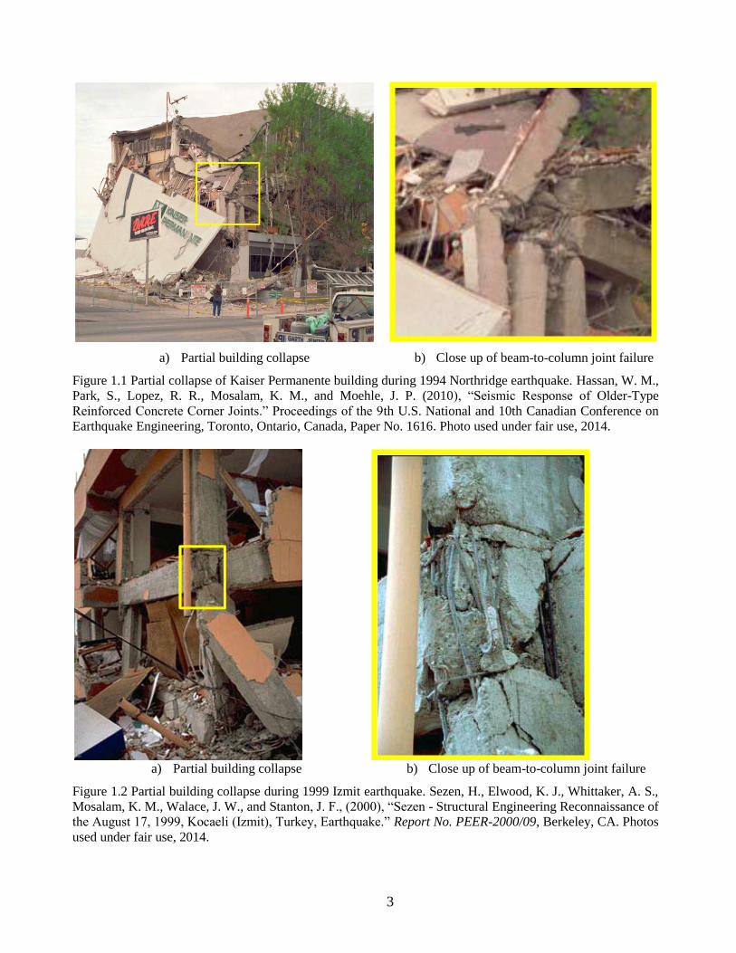
and Kocaeli (Izmit), Turkey. In the 1994 Northridge earthquake there were several building

collapses, including the collapse of the Kaiser Permanente building pictured in Figure 1.1. This

collapse can be traced primarily to the failure of the nonductile beam-to-column connection in

2

the building corner, as seen in Figure 1.1b (Hassan et al., 2010). Figure 1.2 pictures the partial

building collapse of a nonductile RC frame during the 1999 Izmit earthquake in which there is

relatively little damage within the framing elements, but high damage within the beam-to-

column joint (Sezen et al., 2000). The series of earthquakes that struck Christchurch, New

Zealand, from 2010-2012 are another reminder of the massive damage and loss of life that can be

caused by the inadequate performance of poorly detailed RC structures. Several nonductile RC

frames showed signs of damage within the beam-to-column joints and this damage contributed to

the partial or full collapse of certain buildings (Leon et al., 2014).

Nonductile RC frames, having been the norm of construction prior to the advent of

system ductility requirements in the 1971 American Concrete Institute (ACI) building code

(ACI, 1971), comprise a large portion of the existing structures in the U.S. In California alone,

there is an estimated 40,000 nonductile concrete buildings (Comartin et al., 2008), in spite of

relatively frequent significant seismic events. In the Central and Eastern U.S., where significant

seismic events are less frequent, this number increases dramatically. Though they are less

frequent in this part of the country, the extent of a significant seismic event would be much more

devastating due to the lessened capability of the bedrock to disperse seismic energy. Compared

with the 1994 Northridge earthquake, which had a magnitude of 6.7, the magnitude 6 earthquake

that struck Saint Louis in 1895 had a much farther reaching area of damage, as seen in Figure

1.3. If a similar earthquake were to strike the Central or Eastern U.S. today, the results would be

disastrous (Filson et al., 2003).

The high vulnerability of nonductile RC frames to earthquake events forces the

consideration of applying seismic retrofits to existing structures. A rational retrofit strategy

requires the reliable determination of the vulnerability corresponding to a given level of seismic

3

a) Partial building collapse b) Close up of beam-to-column joint failure

Figure 1.1 Partial collapse of Kaiser Permanente building during 1994 Northridge earthquake. Hassan, W. M.,

Park, S., Lopez, R. R., Mosalam, K. M., and Moehle, J. P. (2010), “Seismic Response of Older-Type

Reinforced Concrete Corner Joints.” Proceedings of the 9th U.S. National and 10th Canadian Conference on

Earthquake Engineering, Toronto, Ontario, Canada, Paper No. 1616. Photo used under fair use, 2014.

a) Partial building collapse b) Close up of beam-to-column joint failure

Figure 1.2 Partial building collapse during 1999 Izmit earthquake. Sezen, H., Elwood, K. J., Whittaker, A. S.,

Mosalam, K. M., Walace, J. W., and Stanton, J. F., (2000), “Sezen - Structural Engineering Reconnaissance of

the August 17, 1999, Kocaeli (Izmit), Turkey, Earthquake.” Report No. PEER-2000/09, Berkeley, CA. Photos

used under fair use, 2014.

4

demand, the latter expressed in terms of a deformation history. The aim of this research is to

computationally assess the performance of existing nonductile RC frames undergoing seismic

loads to determine the degree and necessity of seismic retrofits.

1.2 Thesis Scope

This thesis aims to the establishment of a modeling approach that adequately describes

the behavior of nonductile beam-to-column joints. Whereas a great deal of research has been

undertaken to assess the performance of well-detailed joints under cyclic loading, the prevalence

of poorly-detailed joints necessitates an effort to properly model their behavior. Beam-to-column

joint damage is typically caused by shear stresses within the joint which leads to diagonal

Figure 1.3 Damage areas of the 1994 Northridge earthquake and the 1895 St. Louis earthquake. Filson, J.

R., McCarthy, J., Ellsworth, W. L., and Zoback, M. L. (2003), “The USGS earthquake hazards program in

NEHRP—Investing in a safer future.” USGS Fact Sheet 017-03, Reston, VA. Figure used under fair use,

2014.

5

cracking and crushing of the concrete along principal stress planes, and is manifested as spalling

of the concrete on the joint core surface, as pictured in Figure 1.4. Tests have shown that the

concrete compressive strength and confinement,

the steel reinforcement details, and the bond

strength have significant influence on joint

behavior, and the compressive strut and panel

truss have both been described as primary shear

force transfer mechanisms.

The vast majority of analytical models

currently available are either empirical in nature,

and thus should not be applied to cases not

directly related to the physical testing on which

they are based, or mechanistic, based primarily

on considerations of mechanics. The mechanistic

model described herein represents behavior by

nonlinear truss elements, directly modeling steel,

concrete, and reinforcement bond-slip elements

based on their respective cyclic constitutive relationships, and capturing the two primary shear

force transfer mechanisms by assembling these elements into a truss structure. The modeling

scheme has been implemented in the OpenSees analysis platform (McKenna et al., 2005). A

nonlinear steel constitutive model by Dodd and Restrepo-Posada (1995) has also been

implemented to improve on the accuracy of the standard bilinear models used for steel

reinforcement.

Figure 1.4 Concrete spalling within

beam-to-column joint core. Pantelides,

C., Hansen, J., Nadauld, J., and

Reaveley, L. (2002), “Assessment of

Reinforced Concrete Building Exterior

Joints with Substandard Details.”

Report No. PEER-2002/18, Berkeley,

CA. Photo used under fair use, 2014.

6

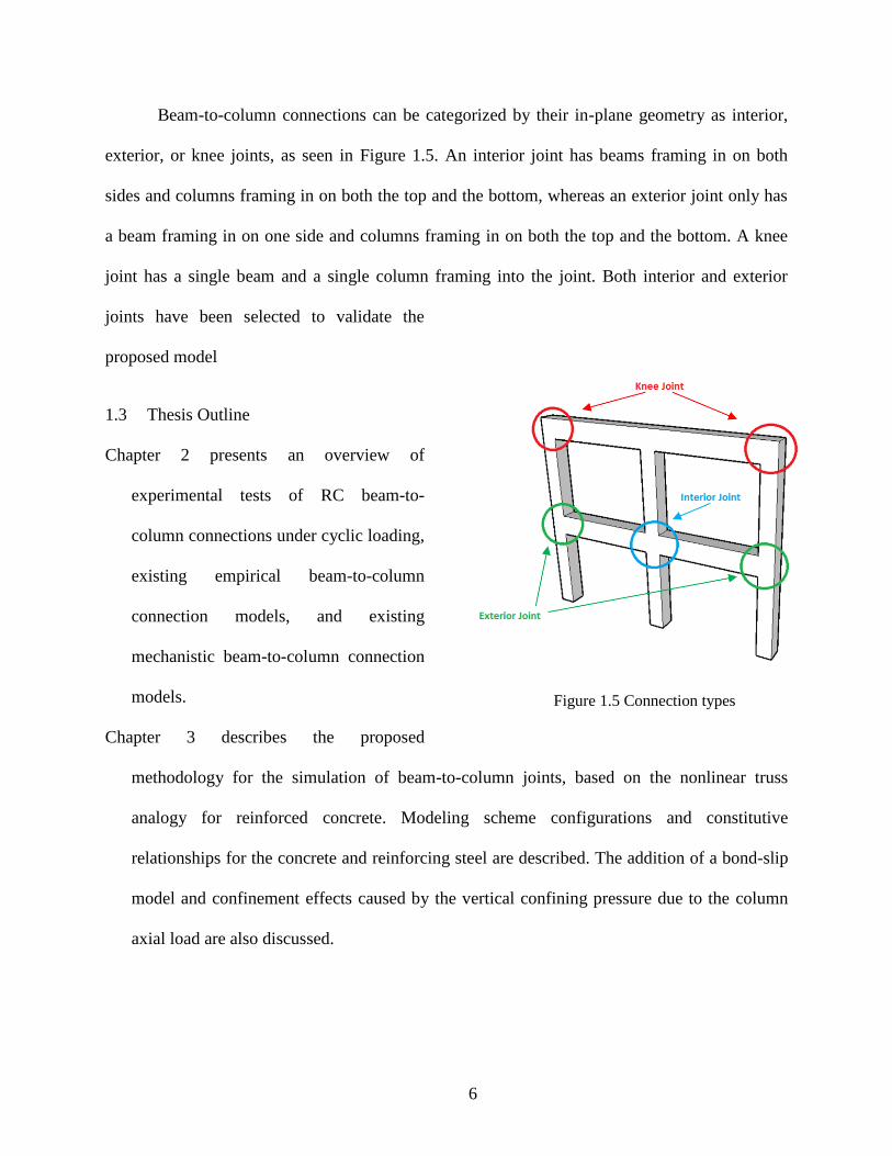
Beam-to-column connections can be categorized by their in-plane geometry as interior,

exterior, or knee joints, as seen in Figure 1.5. An interior joint has beams framing in on both

sides and columns framing in on both the top and the bottom, whereas an exterior joint only has

a beam framing in on one side and columns framing in on both the top and the bottom. A knee

joint has a single beam and a single column framing into the joint. Both interior and exterior

joints have been selected to validate the

proposed model

1.3 Thesis Outline

Chapter 2 presents an overview of

experimental tests of RC beam-to-

column connections under cyclic loading,

existing empirical beam-to-column

connection models, and existing

mechanistic beam-to-column connection

models.

Chapter 3 describes the proposed

methodology for the simulation of beam-to-column joints, based on the nonlinear truss

analogy for reinforced concrete. Modeling scheme configurations and constitutive

relationships for the concrete and reinforcing steel are described. The addition of a bond-slip

model and confinement effects caused by the vertical confining pressure due to the column

axial load are also discussed.

Figure 1.5 Connection types

7

Chapter 4 gives a validation of the proposed model based on quasi-static experimental tests of

nonductile interior and exterior beam-to-column connections. The effects of bond-slip and

concrete confinement are also investigated.

Chapter 5 presents the conclusions of the present study and provides recommendations for future

research.

8

Chapter 2. Literature Review

2.1 Description of Joint Behavior

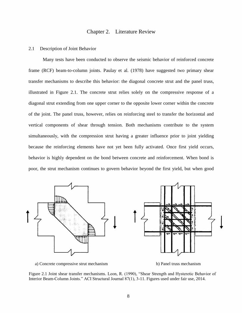
Many tests have been conducted to observe the seismic behavior of reinforced concrete

frame (RCF) beam-to-column joints. Paulay et al. (1978) have suggested two primary shear

transfer mechanisms to describe this behavior: the diagonal concrete strut and the panel truss,

illustrated in Figure 2.1. The concrete strut relies solely on the compressive response of a

diagonal strut extending from one upper corner to the opposite lower corner within the concrete

of the joint. The panel truss, however, relies on reinforcing steel to transfer the horizontal and

vertical components of shear through tension. Both mechanisms contribute to the system

simultaneously, with the compression strut having a greater influence prior to joint yielding

because the reinforcing elements have not yet been fully activated. Once first yield occurs,

behavior is highly dependent on the bond between concrete and reinforcement. When bond is

poor, the strut mechanism continues to govern behavior beyond the first yield, but when good

a) Concrete compressive strut mechanism b) Panel truss mechanism

Figure 2.1 Joint shear transfer mechanisms. Leon, R. (1990), “Shear Strength and Hysteretic Behavior of

Interior Beam-Column Joints.” ACI Structural Journal 87(1), 3-11. Figures used under fair use, 2014.

9

bond is achieved, the panel truss mechanism is dominant.

Ehsani and Wight (1985) tested 6 experiments of exterior beam-to-column joints, varying

the transverse steel reinforcement ratio within the connections. Design values for the joint

transverse reinforcement ratios were calculated based on the draft recommendations of ACI

Committee 352 (ACI, 1985). Actual joints were then built with joint transverse reinforcement

ratios that ranged from 74% to 99% of these design values. The objective was primarily to show

that a less congested joint design may still be adequate in many cases. These tests showed that

the beam-column flexural strength ratio had a significant effect on the location of the flexural

hinge, either well within the beam or in the beam at the column face. For tests with low flexural

strength ratios, where flexural hinges formed in the beam at the face of the column, transverse

reinforcement ratio had little effect. However, when flexural hinges formed well within the

beam, the transverse reinforcement ratio significantly improved the ductility of the joint. Loss of

shear stiffness within the joint was largely attributed to slipping of the reinforcing bars. This

issue was exacerbated by the formation of flexural hinges near the column faces.

Leon (1989) performed four half-scale tests to assess the effects of variable anchorage

lengths and nominal joint shear stress on joint performance. The importance of capturing shear

force-deformation behavior was emphasized, as it has a high influence on joint behavior when

the beam steel development length is less than 24 bar diameters. Leon (1990) suggested that this

shear behavior was highly dependent on the level of bond between the anchored reinforcement

and the concrete, as well as the amount of contact between the joint and the beam at the interface

of the two. For joints with little or no joint transverse reinforcement, he found that the diagonal

compressive strut was the primary shear force transfer mechanism.

10

The effects of cyclic loading on interior and exterior beam-to-column joints of gravity

load-designed frames have been experimentally investigated by Beres et al. (1991, 1992, 1996).

Their tests have shown that the column axial load had a significant influence on the joint

behavior. In the interior joints, this load had a positive effect, with higher compressive loads

leading to increased stiffness and capacity. It was noted that this increased vertical compressive

force within the joint improved the bond between concrete and reinforcement. In the exterior

joints, however, the existence of column axial load precipitated the propagation of shear cracks

within the joint. Column longitudinal reinforcement diameter, quantity, and arrangement were

shown to have little effect on joint behavior. The presence of transverse beams loaded in

compression had a negligible effect in interior joints, but did affect the behavior of exterior

joints. In joints with discontinuous beam longitudinal reinforcement, pull out of the embedded

beam steel was a major contributing factor to failure. It was also noted that spalling of concrete

on the face of the joint lead to the buckling of column longitudinal reinforcement.

Pagni and Lowes (2004) compiled 21 specimen results from 5 sets of experimental tests

to identify damage state development in nonductile reinforced concrete frames during seismic

excitations and potential repair methods to restore the frames to pre-damaged states. The study

found that the following factors have the greatest influence on cyclic joint response: nominal

joint shear stress demand, transverse steel ratio, bond stress demand of longitudinal beam

reinforcement, embedment of beam reinforcement, column axial load, and column splice

location. A total of ten damage states were identified:

1. Flexural cracking at the beam-joint interface,

2. Cracking within the joint,

3. Yielding of longitudinal beam reinforcement,

11

4. Spalling of concrete at joint surface,

5. Deterioration of joint shear strength

6. Extension of joint cracks into beam and/or column,

7. Concrete crushing in joint core,

8. Buckling of column longitudinal reinforcement,

9. Loss of beam longitudinal reinforcement anchorage within the joint core,

10. Pull-out of beam longitudinal reinforcement.

After the onset of joint surface spalling, joint shear strength begins to degrade. Pagni and

Lowes suggest that yielding of longitudinal beam reinforcement has a great influence on

deterioration of bond strength because of the Poisson effect; tensile lengthening of the

reinforcement in the longitudinal direction causes a reduction of cross section in the transverse

directions.

A large database (139 connections) has been constructed by Kim and LaFave (2006) to

allow the detections of common characteristics among these experiments and facilitate the

calibration of analytical models. Experiments included interior, exterior, and knee joints and the

following five parameters were investigated:

1. Concrete compressive strength

2. Joint panel geometry (characterized by the ratios of beam height to column width and

beam depth to column depth)

3. Confinement of joint by beam longitudinal, column longitudinal, and joint transverse

reinforcement

4. Column axial compression

5. Bond demand level of the beam and column longitudinal reinforcement

12

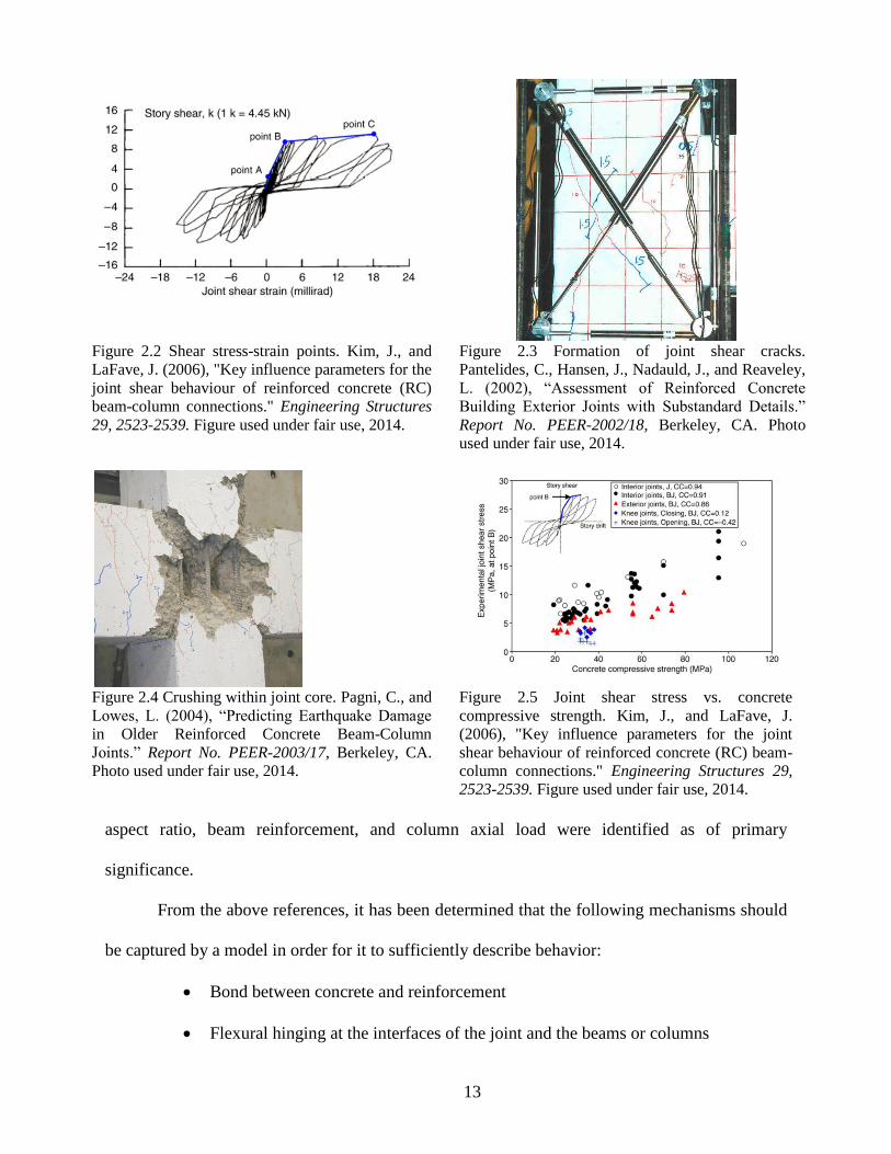
As joint shear strength was the primary focus of the study, all five parameters were

compared with either the joint shear stress or the joint shear strain at three distinct points,

illustrated in Figure 2.2. The first point (point A) was taken as the point of first significant

change in tangent stiffness, considered to be the onset of joint shear cracking, pictured in Figure

2.3. Point B was taken as the point of next significant change in tangent stiffness, assumed to be

caused by a yielding of the joint reinforcement. Point C was taken as the point of maximum

shear stress, at which the initiation of concrete crushing is likely occurring, leading to the

extreme concrete crushing seen in Figure 2.4. It was found that the concrete compressive

strength had the greatest influence on joint shear strength, as seen in Figure 2.5, with the

correlation coefficients between the concrete compressive concrete and the joint shear strength in

certain types of joints exceeding 0.9. It was also noted that the compressive strength affects the

bond formed between concrete and reinforcement, having an added effect on behavior.

Confinement of the joint was also shown to be of some importance, though not as critical as

compressive strength. However, axial load in the column, bond of the longitudinal

reinforcement, and joint geometry were shown to have minimal effect. As this study focused

largely on well confined joints with at least some transverse reinforcement, it is suspected that

findings concerning the negligible effect of reinforcement bonding (and subsequently column

axial load, as this has an effect on bond level) may not be applicable. The high influence of

compressive strength and confinement may be of significance, however.

Park and Mosalam (2009) have examined the results of sixty two tests to determine the

major factors affecting the shear strength of nonductile exterior beam-to-column joints and to

develop both empirical and mechanistic models to predict joint behavior. The effects of joint

13

aspect ratio, beam reinforcement, and column axial load were identified as of primary

significance.

From the above references, it has been determined that the following mechanisms should

be captured by a model in order for it to sufficiently describe behavior:

Bond between concrete and reinforcement

Flexural hinging at the interfaces of the joint and the beams or columns

Figure 2.2 Shear stress-strain points. Kim, J., and

LaFave, J. (2006), "Key influence parameters for the

joint shear behaviour of reinforced concrete (RC)

beam-column connections." Engineering Structures

29, 2523-2539. Figure used under fair use, 2014.

Figure 2.3 Formation of joint shear cracks.

Pantelides, C., Hansen, J., Nadauld, J., and Reaveley,

L. (2002), “Assessment of Reinforced Concrete

Building Exterior Joints with Substandard Details.”

Report No. PEER-2002/18, Berkeley, CA. Photo

used under fair use, 2014.

Figure 2.4 Crushing within joint core. Pagni, C., and

Lowes, L. (2004), “Predicting Earthquake Damage

in Older Reinforced Concrete Beam-Column

Joints.” Report No. PEER-2003/17, Berkeley, CA.

Photo used under fair use, 2014.

Figure 2.5 Joint shear stress vs. concrete

compressive strength. Kim, J., and LaFave, J.

(2006), "Key influence parameters for the joint

shear behaviour of reinforced concrete (RC) beam-

column connections." Engineering Structures 29,

2523-2539. Figure used under fair use, 2014.

14

Diagonal compressive strut mechanism of joint

Panel truss shear mechanism of joint

2.2 Joint Models

A variety of analytical models have been formulated to describe the behavior of

reinforced concrete beam-to-column joints. Simplified models are either empirical, i.e., they are

meant to reproduce the experimentally observed behavior in terms of joint force/deformation, or

mechanics-based, i.e., they describe the mechanics of the salient response mechanisms. The

former are relatively simple models that rely on calibrated springs to represent behavior,

essentially applying curve fitting to overall joint behavior. They can present good agreement

with the tests on which they are based, but it is unlikely that these models will be extendable to

varying cases. The latter mechanistic models are more appealing because of their potential to be

used in a wide array of settings. These models attempt to capture the individual mechanisms that

describe behavior rather than being calibrated based on a curved fit to the overall joint behavior.

They tend to be limited primarily by generalizing assumptions that neglect certain aspects of

behavior in the name of simplicity. Whereas simplicity can be advantageous, especially in

design, it must not be pursued to the detriment of accuracy.

2.2.1 Empirical Joint Models

Alath and Kunnath (1995) developed a simple empirical joint model based on the

experiments of Beres et al. (1992). This model employs a single spring at the intersection of the

beam and column centerlines with rigid end zones in the immediate vicinity of the joint, as seen

in the scissor model in Figure 2.6. A tri-linear shear vs. strain model is used to define the

nonlinear behavior, and the effects of reinforcement, bond-slip, confinement, or concrete

behavior are not explicitly accounted for.

15

Biddah and Ghobarah (1999)

described the effects of shear deformation

and bond-slip with separate spring elements.

For the simulation of an interior joint, two

bond-slip springs and one shear spring were

required, as shown in Figure 2.7. For the

simulation of an exterior joint, one bond-slip

spring and one shear spring represent behavior. An idealized tri-linear constitutive model was

described based on a softening truss model for monotonic behavior, while cyclic behavior was

defined by a multi-linear hysteretic model that neglected pinching due to concrete cracking and

crushing of concrete immediately surrounding reinforcement. These constitutive models are not

deemed sufficient to describe material behavior.

Pampanin et al. (2003) developed a scissor model similar to the one proposed by Alath

and Kunnath (1995), but also included lumped plasticity at the beam ends. The moment-rotation

constitutive model for the joint was based on bilinear shear deformation-principal tensile stress

relationships. The major improvement over Alath and Kunnath (1995) was the inclusion of

pinching in the hysteretic behavior due to bond-slip and shear cracking within the joint.

Anderson et al. (2008) developed a more involved scissor model based on experimental

tests carried out at the University of Washington. A tri-linear envelope representing 3 distinct

levels of stiffness was combined with a multi-linear cyclic model, which had the ability to

include degradation of stiffness and strength. This model also lacks objectivity and extrapolation

of results to more general cases is not advisable.

Figure 2.6 Scissor model

16

Park and Mosalam (2009) developed a semi-empirical moment-curvature relationship

that is applied to a scissor model based on a single diagonal compression strut to resist joint

shear. Joint strength is calculated as a function of the joint aspect ratio and the amount of

longitudinal beam reinforcement (classified by the beam reinforcement index), neglecting

column axial load. Joint aspect ratio is the only parameter affecting maximum and minimum

joint shear strength, but between these values the shear strength is linearly proportional to the

beam reinforcement index. This model was only developed for exterior and knee joints.

Birely et al. (2011) proposed a model with a rigid joint with rigid offsets, at the end of

which there are two springs connected in series to the beams on either side of the joint, as seen in

Figure 2.8. The model incorporates a lumped-plasticity beam-column element with the two

springs representing the moment-rotation response of the joint and the moment-rotation response

of the beam. No consideration is made for nonlinearity in the column. Eleven different research

regimens totaling 45 different beam-to-column joint specimens, which all used normal weight,

non-high-strength concrete in interior joints, were used to calibrate the model. It was not

considered appropriate to extend this model to further specimen types.

Figure 2.7 Joint model by Biddah and Ghobarah

(1999)

Figure 2.8 Joint model by Birely et al. (2011)

17

2.2.2 Mechanistic Joint Models

Filippou et al. (1983) proposed an analytical joint model similar to a fiber section beam

model, as seen in Figure 2.9. The cross section of the joint was divided into several layers, each

representing either steel reinforcement or concrete. Nonlinear constitutive models were used to

represent the behavior of these layers, with the Menegotto-Pinto relationship representing steel

and a model developed by Filippou representing the concrete. This concrete model bases crack

closure (and thus the onset of regaining compressive strength) on the crack width in a given

layer, but does not account for any tensile strength in the concrete. A bond stress-slip model

developed by Ciampi et al. (1981) is used to account for the incompatibility of steel and concrete

strains. Thus, the model by Filippou et al. (1983) can handle the effects of bond-slip and concrete

flexural cracking; however, it does not account for any of the effects of shear within the joint and

thus is ultimately deemed unsatisfactory.

An analytical model utilizing the modified compression field theory (MCFT), pictured in

Figure 2.10, has been developed by Lowes and Altoontash (2003). This model defines a 4-sided

shear panel based on MCFT connected to 4 rigid interface members. The panel-interface

Figure 2.9 Joint model by Filippou et al. (1983) Figure 2.10 General model used by Lowes,

Altoontash, and Mitra

18

connection is accomplished through 3 zero-length spring elements on each side: one at each

corner to represent bar-slip behavior and one at the center to represent beam-joint interface shear.

The elastic interface shear spring accounts for crack openings at the faces of the joint. A bar

stress vs. slip relationship, shown in Figure 2.11, was developed for this model primarily based

on experiments conducted by Lowes (1999) and Eligehausen et al. (1983). Bar stress increases

fairly quickly until the steel yields, at which

point there is a dramatic decrease in stiffness.

Once the slip reaches the “slip limit” of 0.1

in. (3mm), strength decreases linearly to the

residual stress. As can be seen in the

comparison of the bond-slip model to test

results in Figure 2.12, this model has decent

agreement with cyclic behavior, though it has

poor agreement under monotonic loading. A

single multi-linear uniaxial load-deformation

model was developed to describe the

hysteretic behavior of the various materials.

By varying the input parameters, constitutive

relationships were defined for the shear panel

and the bar-slip. The shear panel is treated as

a single entity, thus giving it a sort of “black

box” nature that does not allow for the

extraction of information about individual

Figure 2.11 Lowes and Altoontash (2003) bond-slip

envelope curve

a) Simulated results

b) Experimental results

Figure 2.12 Verification of bond-slip model. Lowes, L.,

Mitra, N., and Altoontash, A. (2004), “A Beam-

Column Joint Model for Simulating the Earthquake

Response of Reinforced Concrete Frames.” Report No.

PEER-2003/10, Berkeley, CA. Figures used under fair

use, 2014.

19

contributions to failure. The use of MCFT assumes at least a moderate amount of transverse

reinforcement within the joint.

Mitra and Lowes (2007) refined the Lowes and Altoontash (2003) model by making

three major adjustments: replacing MCFT with a diagonal compression-strut mechanism to

represent the shear panel, slightly altering the placement of the bond-slip springs to better

represent true specimen geometry, and altering the constitutive model for the bond-slip springs.

The concrete strut within the joint carries the entire shear load. The contribution of steel

reinforcement is only considered in relation to confinement of the core; the only relation of steel

to the model is the resultant force orthogonal to the compression strut. No consideration is made

for axial deformations or buckling of the reinforcement. The constitutive model for the springs

was altered so that convergence issues in computation could be avoided. In the Lowes and

Altoontash model, the loss of strength due to reaching the slip limit would result in a negative

slope. In this model, however, the loss of strength is handled by the hysteretic model. As the

model is cycled to increasing slip, the stiffness is decreased so that a higher amount of slip

results in lower bond forces.

As these models (Lowes and Altoontash, 2003, and Mitra and Lowes, 2007) were

developed to be used more with modern RC beam-to-column connections, it was assumed that

the joints are well confined. For this reason, these models are not considered suitable for the

analysis of joint in old, poorly detailed RC frames.

Shin and LaFave (2004) suggested a rectangular joint subassembly consisting of rigid

links pinned at the corners, as seen in Figure 2.13. One corner is assigned three bilinear

rotational springs superimposed to represent shear behavior. Rotational springs are also placed at

the joint-beam interfaces to represent bond-slip. The three shear springs are combined to create a

20

multi-linear envelope based on MCFT and

hysteretic behavior calibrated from experimental

data. It was assumed that this model would be

applied to ductile moment frames, for which

MCFT is intended. Assumed confinement of the

joint core gives this model little applicability to

poorly-detailed beam-to-column joints.

Park and Mosalam (2009) developed a model to predict the behavior of exterior joints.

This model assumes beam longitudinal reinforcement is bent at 90°. Two diagonal struts,

illustrated in Figure 2.14, are assumed to resist the entirety of the shear: one between the bend of

the beam reinforcement and the concrete compression blocks in the opposite corner (ST1) and

another between that opposite corner and the concrete surrounding the horizontal portion of that

same beam reinforcement (ST2). This latter strut is a result of the bond between the

reinforcement and the concrete. Joint shear failure is assumed to initiate at the node of the upper

beam reinforcement bend because this is where anchorage of that reinforcing bar is assumed and

is the location of greatest crack width. A fraction factor, α, is determined to define the

contribution of ST1 to shear resistance, while the remainder is attributed to ST2. To represent

bond deterioration, as tensile stress increases in the beam reinforcement, α increases. As in the

phenomenological model by Park and Mosalam (2009) described earlier, this model was

designed only for exterior joints and confinement in the joint and axial load in the column are

neglected.

A joint model based primarily on the principal tensile stress has been proposed by

Sharma et al. (2011). This model, pictured in Figure 2.15, combines 3 hinges with a centerline

Figure 2.13 Joint model by Shin and LaFave (2004)

21

model to describe behavior of exterior beam-to-column joints. Two constitutive models were

developed to relate the principal tensile stress and the shear deformation within the joint: one

relationship for joints with both top and bottom beam reinforcement bars bent in and one for

joints with top beam reinforcement bent in and bottom beam reinforcement embedded 6 in.

straight into the joint. These constitutive relationships are illustrated in Figure 2.16. The

relationships of beam moment to joint shear strain and column shear to joint shear strain (and

thus to the deformation at the joint-column interface) are found through an iterative procedure

using the aforementioned principal tensile stress-shear deformation constitutive relationships. In

order to extend this model to further joint types, additional principal tensile stress-joint shear

deformation relationships must be developed. Bond-slip in the model is not directly modeled. It

also does not allow for the evaluation of the causative effects of individual components to

failure.

More refined 2-dimensional finite element models have been pursued (Noguchi, 1981,

Pantazopoulou and Bonacci, 1993, Kashiwazaki et al., 1996, Baglin and Scott, 2000). These

models utilize 2-dimensional quadrilateral or triangular elements to represent concrete, along

Figure 2.14 Diagonal struts of mechanistic

joint model by Park and Mosalam (2009)

Figure 2.15 Joint model by Sharma et al. (2011)

22

a) Both beam reinforcement bars bent in b) Top beam bar bent in, bottom beam bar

embedded 6 in straight into joint

Figure 2.16 Principal tensile stress-joint shear deformation constitutive relations. Sharma, A.,

Eligehausen, R., and Reddy, G. (2011), “A new model to simulate joint shear behavior of

poorly detailed beam-column connection in RC structures under seismic loads, Part I: Exterior

joints.” Engineering Structures 33, 1034-1051. Figures used under fair use, 2014.

with biaxial constitutive relationships, and either 2-dimensional or truss elements to represent

reinforcing steel. Bond-slip and concrete cracking, if accounted for explicitly, are modeled using

zero-length contact elements or, in the case of concrete cracking, smeared crack elements. In

order to accurately traverse highly nonlinear constitutive relationships, some models, such as the

one seen in Figure 2.17 require up to 100 concrete elements within the joint panel alone. Cyclic

loading is not conducted with these models because of the high computational expense. In

monotonic loading, these models do not capture well the degradation in the response after joint

shear cracking, as shown in Figure 2.18. The computational expense and complexity of such

models makes them difficult to implement when modeling the overall response of a building

structure.

23

Figure 2.17 Finite element model. Pantazopoulou, S. J., and Bonacci, J. F.

(1994), “On earthquake-resistant reinforced concrete frame connections.”

Canadian Journal of Civil Engineering 21, 307-328. Figure used under fair

use, 2014.

Figure 2.18 Load-deflection response of finite element joint model

compared with measured response. Baglin, R. H., and Scott, P. S. (2000),

“Finite Element Modeling of Reinforced Concrete Beam-Column

Connections.” ACI Structural Journal 97(6), 886-894. Figure used under

fair use, 2014.

24

Chapter 3. Analysis Methodology

3.1 Introduction

An RC beam-to-column joint model must adequately capture physical joint behavior. In

the case of mechanistic models, the applicable force transfer mechanisms and material properties

must be included to attain model accuracy. The force transfer mechanisms within beam-to-

column joints include: bond-slip between concrete and reinforcing steel, the diagonal

compression strut, and the panel truss. The existing mechanistic models described previously

rely, in one form or another, on broad simplifying assumptions that neglect aspects of these force

transfer mechanisms. In some cases, these assumptions neglect shear deformations all together.

In others, they do not adequately capture the effects of the shear failure mechanisms in poorly

detailed joints.

The model proposed herein relies on a nonlinear truss structure to capture the diagonal

components of the diagonal compressive strut and panel truss shear transfer mechanisms. Zero-

length springs connecting steel and concrete elements capture the reinforcement bond-slip

relationship. Concrete truss elements are defined by a nonlinear concrete constitutive stress-

strain model developed and a new implementation of a uniaxial stress-strain law for steel

reinforcement is used to define the steel truss elements.

3.2 Description of Nonlinear Truss Analogy for Beam-to-Column Joints

The modeling approach is based on the work of Panagiotou and Restrepo (2011).

Diagonal concrete elements represent the primary shear resistance mechanism, with vertical and

horizontal concrete and steel elements to account for axial resistance. The bond-slip is modeled

with nonlinear zero-length springs connecting the concrete and steel elements. A general layout

25

of the model applied to an interior beam-column joint is shown in Figure 3.1d, along with the

hypothetical joint that it would represent, shown in Figure 3.1a. Horizontal and vertical concrete

elements create many truss cells, each of these cells containing two orthogonal diagonal concrete

struts. An example of one of these cells is given in Figure 3.1b and the size of these cells will

henceforth define the mesh size of the model. It is advantageous to have these cells as close to

square as possible, for reasons that will be explained below.

For ease of modeling, it is suggested that the mesh size remain constant within a joint

model. The mesh size will thus be defined as a fraction of the size of the joint core, which is

bounded top and bottom by the beam reinforcing bars and left and right by the outer column

reinforcing bars. This can be seen in Figure 3.1c, which shows the truss assemblage of an

exterior joint superimposed on its reinforcing schematic. The outer longitudinal beam and

column reinforcing bars must be modeled so that they exactly overlay the physical specimen,

otherwise the effective diagonal compressive strut will not be appropriately defined and will vary

depending on the mesh size.

The cross-sectional areas of the steel truss elements are calculated based on the amount of

reinforcing steel in the system. As is illustrated in Figure 3.1c, the transverse reinforcing steel

elements do not exactly overlay the physical specimen. To account for this, the cross-sectional

areas of the transverse steel elements are determined in order to give the correct transverse

reinforcing steel ratio. As the longitudinal steel elements are modeled exactly, their areas can be

taken directly from the physical specimen.

26

The cross-sectional areas of the concrete truss elements are obtained as the product of the

tributary width and of the out-of-plane thickness, w. The effective width of diagonal elements,

beff, is determined from the vertical component, b, and horizontal component, a, of the element

such that:

, as illustrated in Figure 3.1b. The area of the diagonal elements then

b) Concrete truss

cell

c) Exterior joint truss assemblage over

specimen reinforcing schematic

a) Interior joint physical layout

d) Corresponding components of interior joint model layout

Figure 3.1 Proposed model layout

27

becomes . For horizontal and vertical concrete elements, the effective width is

found as the tributary width of a given element. The cross sectional area of the cover concrete is

included in the horizontal and vertical concrete elements that coincide with the exterior

longitudinal steel reinforcement.

The interface of the joint and the adjacent beam or column is modeled as a rigid beam-

column element. This is done in order to maintain the assumption that within the beams and

columns plane sections remain plane and perpendicular to the deformed centerline of that

framing element.

3.2.1 Concrete Model

The concrete elements are defined using the constitutive model proposed by Lu and

Panagiotou (2013) found in Figure 3.2. The model has been defined for both confined and

unconfined concrete. In confined concrete, two distinct branches are defined in compression

prior to reaching the compressive strength: a quadratic curve up to the unconfined compressive

Figure 3.2 Lu and Panagiotou (2013) uniaxial stress-strain law for concrete

28

strength, f’c, at the unconfined peak strain, εo, followed by a cubic curve up to the confined

compressive strength, fcc. There is then a plateau extending from the confined peak strain, εco, to

the ultimate compressive strain, εcs. This is followed by linear softening to zero stress at a strain

of εcu. Unconfined concrete follows the same path up to the unconfined compressive strength, at

which point linear softening occurs until stress is reached at a strain of εu. Unloading from

compression is accomplished by a nonlinear curve until zero stress is reached. Once zero stress is

reached, a linear branch extends to the point of maximum prior tensile strain, and then the

tension curve is rejoined.

The tensile response of the model is equivalent for both confined and unconfined

concrete. The response is elastic until cracking, which is defined by the tensile strength of the

concrete. For horizontal and vertical concrete elements the tensile strength is assumed to be

ct ff '33.0 (ft and f’c in MPa), whereas the diagonal concrete elements have no tensile

strength. Following the elastic branch, a sharp peak leads to softening either by tension stiffening

or as defined by a tri-linear relationship (not shown). Unloading in tension is comprised of three

linear branches. The first has a slope equivalent to the initial modulus, Ec, and is defined from

the point of reversal to the point of zero stress. The second branch extends down to a point of

zero strain and a stress of -αft, where α = 0.5. The final branch reconnects to the point of

maximum prior compressive strain, at which point the compressive skeleton curve is rejoined.

The performance of nonlinear structural elements with softening branches is highly

dependent on the element mesh length (see Panagiotou et al., 2012, for further details). To

account for this mesh size effect, the compressive degrading branch is made steeper as the

element length increases. This is accomplished by altering the values of εu in unconfined

concrete and εcu in confined concrete.

29

3.2.2 Transverse Strain Effect in Concrete

For diagonal concrete

elements, transverse strain effect is

taken into account as per Vecchio and

Collins (1986). As transverse strain,

εn, is increased in the tensile

direction, the compressive strength of

the material decreases according to

the multiplier β. β is defined by a tri-

linear relationship with the transverse

strain, as seen in Figure 3.3. Compressive (negative) values of εn give a β value of 1 and thus

have no effect on behavior. In order to measure transverse strain, four nodes must be defined for

a single element. From these four nodes, two will define a concrete truss element and two will

define a zero-stiffness gauge element, also pictured in Figure 3.3. It is advised to define the two

transverse gauge nodes at locations that will give an orthogonal gauge element in order to

produce an accurate approximation of εn. In general, as the diagonal elements are part of a cell,

the two transverse nodes will be taken as the remaining two nodes in the cell. For this reason, it

is advantageous to create a close-to-square meshing of the concrete. The effect of element length

is also accounted for in the transverse strain effect. As the length of the concrete strut element

increases, the values of εint and εres decrease.

3.3 Enhancements to Truss Modeling Approach for Beam-to-Column Joints

Three enhancements have been made to the nonlinear truss analogy modeling scheme for

beam-to-column joints. Confining pressure due to column axial load is used to calculate the

Figure 3.3 Transverse strain strength reduction factor

30

confinement parameters of concrete, a new uniaxial stress-strain law for reinforcing steel is

implemented to improve accuracy, and the bond-slip effect is included by the use of zero-length

springs.

3.3.1 Effective Concrete Confinement Due to Axial Column Load

It has been observed (Paulay and Scarpas, 1981, Beres et al., 1996, Pantelides et al.,

2002) that column axial load has a positive effect on strength and ductility of beam-to-column

connections. To account for this effect, the value of column axial stress, fa, is used to define the

partial confinement of certain concrete elements. Figure 3.4a shows a concrete core with a

vertical column axial stress applied to it. This stress is assumed to have a confining effect on

both horizontal and diagonal elements.

The confining pressure for horizontal

elements is taken as fa and for diagonal

elements it is taken as , where

θ is the angle of inclination for that

element, as seen in Figure 3.4. The

confined compressive strength, fcc, and

strain, εco, are found based on the

expressions of Mander et al. (1988)

and follow the equations:

c

tr

c

trccc

f

f

f

fff

'2

'

94.71254.2254.1' (Eq 3.1)

1

'51

c

ccoco

f

f (Eq 3.2)

Figure 3.4 Concrete confinement pressure

a) Joint core confined by column axial stress,

b) Level of confinement in horizontal elements,

c) Level of confinement in diagonal elements

31

cosa

a

trf

ff (Eq 3.3)

where ftr is the transverse confining pressure. The ultimate concrete compressive strain, εcs, is set

equal to εco. This is because the plateau in the model proposed by Mander et al. (1988) is meant

to extend to the point when the first confining hoop fractures, whereas there are no confining

hoops within the joints of the specimens investigated in this study.

3.3.2 New Implementation of a Uniaxial Model for Steel Reinforcement

The stress-strain constitutive models developed for reinforcing steel to date are either

overly simple or else difficult to calibrate to test data. The typical bilinear models, such as the

Menegotto-Pinto stress-strain law for reinforcing steel, give a poor representation of behavior,

with no distinction made between the yield plateau and strain hardening regime. Those models

that do account for this distinction are calibrated based on the initial strain hardening modulus,

which can be difficult to determine from test data. For these reasons, the constitutive law for

steel proposed by Dodd and Restrepo-Posada (1995) has been selected for the reinforcing

elements and has been implemented as the uniaxial material model DoddRestr in the OpenSees

analysis platform (McKenna et al. 2005). It is an accurate model that requires a fairly limited

number of parameters to be calibrated. The elastic region, yield plateau, nonlinear strain

hardening, and post-peak softening are all defined within the skeleton curve. The Bauschinger

effect (captured within the nonlinear Bauschinger branch) is also accounted for within multiple

different types of unloading and reloading curves. The key features of this model can be found in

Figure 3.5.

In order to account for differences between the compressive and tensile portions of the

curve, this model operates within the natural coordinate system. Whereas the engineering

coordinate system assumes a constant cross section and length to define the stress and strain of

for horizontal elements

for diagonal elements

32

an element, the natural coordinate system is based on the instantaneous cross section and length

of the reinforcement. These instantaneous parameters are calculated assuming that the element

maintains constant volume as it is stretched or compressed. By basing the reinforcement stress

on the instantaneous cross section, increased compressive strength can be accomplished.

The material parameters are entered in engineering stress-strain space. The model then

converts the inputs to natural coordinates to perform the constitutive operations before

converting the output parameters (stress and tangent modulus) back to engineering coordinates.

Natural strain is related to engineering strain as:

)1ln(' (Eq 3.4)

And natural stress is related to engineering stress as:

)1(' (Eq 3.5)

As shown in Figure 3.5a, the skeleton curve consists of three major branches: the linear

elastic portion, the yield plateau, and the strain hardening regime and post-peak softening branch.

The linear elastic portion maintains a constant slope equal to young’s modulus up to the yield

a) Skeleton curve b) Hysteretic behavior

Figure 3.5 Dodd and Restrepo-Posada (1995) constitutive law for steel

33

stress, fy, when the yield plateau is entered. The yield plateau is a zero stiffness region that has a

constant stress equal to fy. εsh then marks the onset of the strain hardening regime, which is

defined as a nonlinear curve that reaches the ultimate strength, fsu, with zero-slope at the ultimate

strain, εsu. The exponent, Psh, used to describe the curve of the strain hardening regime is

calibrated based on an arbitrary point along the curve, (εsh1, fsh1). This allows for a simple and

accurate calibration based on experimental test data. Continued softening of the model beyond

the ultimate strength accounts for the post-peak behavior of the steel, leading to a negative-slope

degrading branch.

Unloading and reloading reversals are distinguished into these categories, namely, major,

minor, and simple, as shown in Figure 3.6. Any unloading branch whose reversal point occurs

within the non-elastic range of the skeleton curve is a major reversal, as seen in Figure 3.6b.

Major reversals are comprised of a linear unloading branch and a nonlinear branch that

represents the Bauschinger effect (the Bauchinger branch). Reversals within the yield plateau

will eventually reconnect to a skeleton curve that has been shifted to account for plastic strains.

Reversals within the strain hardening regime simply target the opposite ultimate stress-strain

point, which has also been shifted to account for plastic strains. Major reversals can also be

triggered within the nonlinear Bauschinger branch of another major reversal if the difference in

stress between the two reversals is greater than 2fy. These types of major reversals behave very

similarly to those which occur within the strain hardening regime.

If a reversal occurs within a major reversal such that the stress difference between the

two reversals is less than 2fy, it is considered a minor reversal, as seen in Figure 3.6c. Minor

reversals are also comprised of a linear branch and a curved Bauschinger branch. There are now

two reversal points of immediate importance: the point from which the minor reversal began

34

(point 2 in Figure 3.6c) and the point from which the major reversal began (point 1 in Figure

3.6c). The major reversal was initiated within either the skeleton curve or another major reversal,

referred to as the master branch. The minor reversal is always aiming to reconnect to the master

branch at point 1. Thus, minor reversals can never cause an increase in the plastic strain of the

reinforcing bar.

Any reversal that occurs within the Bauschinger curve of a minor reversal is classified as

a simple reversal. As with minor reversals, simple reversals have both a linear and a curved

Bauschinger branch and there can also be no increase in plastic strain accrued within a simple

a) Relationships between reversals b) Major reversal load path

c) Minor reversal load path d) Simple and linear reversal load paths

Figure 3.6 Loading reversals

35

reversal. Simple reversals can also be initiated by a reversal within the curved branch of another

simple reversal. These reversals aim to reconnect to either the major reversal from which their

minor reversal initiated from (point 2) or to the master branch (point 1). This can be seen in

Figure 3.6d where the first simple reversal is aiming to reconnect to the major reversal and the

second simple reversal is aiming to reconnect to the master branch.

As has been discussed, all reversals have an initial linear elastic portion. If a reversal

occurs within one of these regions, the model traces back along this linear portion until the prior

reversal point is reached, as seen in Figure 3.6d. Once this reversal point is reached, the previous

branch is rejoined.

The Bauschinger effect for the three types of reversals (major, minor, and simple) is

accounted for using the same nonlinear equation with a differing exponential coefficient: Pmajor

for major reversals and Pminor for minor and simple reversals. Pmajor varies based on the amount

of plastic strain. Because the Bauschinger portion of minor and simple reversals is fairly short,

Pminor was calibrated based on test data and is set as a constant value of 0.35.

The implemented model has been designed to give added control to the user. In order to

allow for a more accurate calibration, the exponential coefficients Pmajor and Pminor have been

included as input parameters. If measurements of the cyclic stress-strain behavior for the

reinforcing steel are taken, the variation of the Pmajor coefficient can significantly improve the

model accuracy.

The implementation of the constitutive law follows the type of branch the model is in at

any given point during cyclic loading: the skeleton curve, major reversals, minor reversals, or

simple reversals loading in either the tensile or compressive directions. This allows for rigorous

model tracking when a reversal occurs, ensuring accuracy when simulating physical behavior.

36

The nonlinear branch representing the Bauschinger effect in the various reversals is solved using

a full Newton-Raphson iterative algorithm. If the Newton-Raphson algorithm is unable to

converge, a simple bisection algorithm is employed to solve the nonlinear equation. The full

source code for this model can be found in Appendix A.

The model has been verified against the results of quasi-static cyclic tests of deformed

reinforcing bars performed by Restrepo et al. (1994). Testing of a 16mm diameter grade 430

steel coupon (HX15) is compared to simulated results in Figure 3.7. Calibrated material

properties can be found in Table 3.1. Good agreement is achieved between the model and the

measured data.

3.3.3 Bond-Slip Model

The reinforcing bar bond force-slip displacement constitutive model chosen was

developed by Mitra and Lowes (2007), as seen in Figure 3.8. Bond-slip is modeled using zero-

Figure 3.7 Measured and simulated cyclic stress-strain response of steel model

Table 3.1 Calibrated Steel Material Properties for Steel Coupon

fy (MPa) fu (MPa) εsh (%) εu (%) Es (GPa) εsh1 (%) fsh1 (%) Pmajor Pminor

450 640 1.2 20 190 3 560 0.1 0.35

37

length translational springs to connect coincident steel and concrete nodes with the uniaxial

material BarSlip, which is available in OpenSees.

There are three distinct, linear branches of the envelope of the model: an elastic branch, a

yielded branch, and a post-ultimate branch. The stiffness of the elastic branch is based on the

elastic modulus of the reinforcing steel. Once first yield of the steel has occurred, the yielded

branch is entered and the stiffness is reduced based on the hardening modulus of the steel,

assuming a bilinear steel stress-strain relationship. This is maintained until the ultimate strength

of the steel is reached, initiating a near-zero-stiffness plateau. Constant positive stiffness is

maintained to aid in model convergence. In tension, the yielded reinforcing bar has very little

bond with the concrete because of Poisson’s effect. Thus, there is very little strength gain after

reinforcing bar yielding occurs and the yielded branch and post-ultimate branch can merge, as is

illustrated in Figure 3.8.

Hysteretic behavior is also comprised of three linear branches: an initial unloading

branch, a very shallow branch to account for material pinching, and a reloading branch, as seen

in Figure 3.8. The material pinching branch is included to represent crushing in the concrete

immediately surrounding the rebar. Material softening is accounted for within the hysteretic

behavior; damage parameters reduce the bond strength based on the maximum deformation

experienced by the material as cycling occurs. More information on this model can be found in

Lowes et al. (2004) and Mitra and Lowes (2007).

38

Figure 3.8 Bond-slip model by Mitra and Lowes (2007)

39

Chapter 4. Validation of Analysis Methodology

Validation of the model described herein is accomplished by comparing the force-

displacement responses of the model to experimental test results. The model was built in the

OpenSees nonlinear structural analysis computer program (McKenna et al., 2005). Two-

dimensional nonlinear static analyses using a Newton-Raphson iterative solution scheme were

performed on a 3.47 GHz Intel Xeon processor and took roughly ten minutes. Quasi-static tests

of beam-column subassemblies detailed to approximate the standards of practice in reinforced

concrete moment frame construction prior to the advent of joint ductility requirements were

selected for this study. Three tests were selected to compare against: two interior beam-column

subassemblages tested by Alire (2002) and an exterior beam-column subassemblage tested by

Pantelides et al. (2002).

4.1 Analysis of Interior Beam-to-Column Joints

The testing scheme of four interior beam-column subassemblages undertaken by Alire

(2002) was intended to support the development of modeling techniques for nonductile beam-to-

column joints. In an earlier study (Mosier, 2000), it was found that moment frame construction

prior to 1967 typically lacked transverse reinforcement within the joints. Thus, Alire

approximated pre-1967 building standards for these tests. Specimens PEER-0850 and PEER-

0995 are selected for this study. The first specimen had good ductility but ultimately failed due

to a combination of slipping of the bond of the beam reinforcing bars and joint shear cracking,

whereas the second specimen had significant shear cracking early in the test and failed due to

crushing within the concrete core.

40

a) Interior joint dimensions

b) Reinforcement detailing for specimen 1 c) Reinforcement detailing for specimen 2

Figure 4.1 Reinforcement detailing of interior beam-column assemblies. Alire, D. (2002), “Seismic

Evaluation of Existing Unconfined Reinforced Concrete Beam-Column Joints.” M.S. Thesis, University of

Washington, Seattle, WA, 306pp. Figures used under fair use, 2014.

4.1.1 Specimen Descriptions

Detailing for both joints can be found in Figure 4.1. They are 2/3 scale planar beam-

column assemblages with no transverse beams framing into the joint. The beams and columns

41

have cross-sectional dimensions of 20”x16” and 18”x16”, respectively, and 1” concrete cover.

The beams and columns were designed to ensure that beam longitudinal steel would yield prior

to column longitudinal steel, maintaining a column moment-to-beam moment flexural strength

ratio (ΣMc/ΣMb) greater than 1.5. Sufficient transverse hoop reinforcement was supplied to

prevent shear failures within the beams and columns, though no transverse reinforcement was

supplied within the joint. Longitudinal reinforcement was continuous from end to end to avoid

splice failures. The specimens were cast and stored horizontally, then lifted into place to be

tested vertically.

The specimens were built with varying concrete compressive strengths and target joint

shear stresses. The first interior specimen was built with normal strength concrete, having a

compressive strength on the day of testing (f’c) of 5,070 psi. The second was built with high

strength concrete with a compressive strength of 8,767 psi. The normalized target joint shear

strengths (vjt/√f’ct) were 5.70 for the first interior joint and 8.50 for the second. The steel

reinforcement for the two specimens was selected to achieve these targets. The beams of the

second interior joint were built significantly stronger than those of first, with longitudinal

reinforcement consisting of five No. 7 bars on top and three No. 7 bars on bottom in the second

interior joint, whereas the first was reinforced with two No. 7 bars top and bottom. The column

reinforcement of the first joint consisted of eight No. 4 bars and the column reinforcement of

second consisted of eight No. 6 bars, spaced evenly as seen in Figure 4.1. With the exception of

the beam-to-column connections, transverse reinforcement was consistently No. 4 bars spaced at

3.5” on center. The reinforcing steel material properties were presented in terms of the Raynor

steel constitutive model (Raynor, 2000). These properties have been calibrated to the Dodd-

42

Restrepo (1995) steel constitutive model and can be found in Table 4.1 along with a comparison

of the model to the experimental data, found in Figure 4.2.

The loading conditions of the two specimens were identical. An axial load of 0.1f’cAg

was applied to the columns. This represented an estimated average of the axial loading that pre-

1967 RC moment frame columns were designed to experience. Cyclic lateral loading was

applied vertically in opposite directions at the beam ends (see Figure 4.4a). Ten different drift

levels were applied, as detailed in Table 4.2. Each subsequent drift loading level was comprised

Table 4.1 Alire Reinforcement Properties

No. 4 bars No. 6 bars No. 7 bars

fy (ksi) 77.8 73.2 73.1

Fu (ksi) 1021.7 123.4 123.5

Es (ksi) 33,190 31,463 31,619

εsh 0.59% 0.66% 0.45%

εu 8% 12% 9%

fsh1 (ksi) 105.9 105.6 108.8 Figure 4.2 Comparison of experimental data to

Dodd-Restrepo steel constitutive model εsh1 3% 3.5% 3.5%

Table 4.2 Alire Displacement History

Drift

Level

Drift

Ratio (%)

Displacement at

Beam End (in)

1 0.1 0.07

2 0.25 0.18

3 0.5 0.36

4 0.75 0.54

5 1 0.72

6 1.5 1.08

7 2 1.44

8 3 2.16

9 4 2.88

10 5 3.60 Figure 4.3 Applied drift history for the

specimens tested by Alire (2002)

43

of three positive and three negative cycles, as seen in Figure 4.3. The drift ratio was calculated as

bL/ , where δ is the vertical displacement at the beam tip and Lb is the length of the beam,

shown in Figure 4.1.

4.1.2 Model Descriptions

The specimens have been modeled similarly for both cases, using single elements for the

beams and columns and a refined joint subassembly. The full model layout, along with the

bounds of the concrete specimen, can be found in Figure 4.4a. The beam and columns have been

modeled with nonlinear force-based beam-column elements. The top node of the upper column

has been fixed against horizontal translation and a load has been applied in the vertical direction

to simulate the axial column load. The bottom node of the lower column has been pinned. The

horizontal reaction at this node will be used to determine the column shear. The lateral cyclic

load will be applied vertically at the outer nodes of both beams, where the positive directions are

as indicated in Figure 4.4a.

The nonlinear truss joint subassembly is detailed in Figure 4.4b and c, with varying steel

and concrete truss element cross-sectional areas given in Figure 4.4b. A four cell by four cell

mesh was selected for the joint cores, leading to a cell height of 4.5”, a cell width of 4”, and an

angle of inclination of 48.4°. Horizontal and diagonal concrete elements are given differing

material properties to represent the appropriate level of vertical confining pressure due to the

column axial load. Vertical concrete elements receive no confining benefit due to the column

axial load. Varying zero-length bond-slip spring material types are dependent on location and

surface area of reinforcing bars at a given reinforcing layer. For the first joint, beam-longitudinal,

column-longitudinal, and transverse steel elements are defined using No. 7, No.4, and No. 4 steel

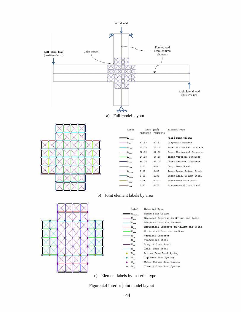
44

a) Full model layout

b) Joint element labels by area

c) Element labels by material type

Figure 4.4 Interior joint model layout

45

reinforcement material properties, respectively; for the second, No. 7, No. 6, and No. 4

reinforcement material properties are used to define these elements, respectively.

The testing equipment used for the test included gauges to measure shear strain. The total

shear strain, denoted as engineering shear strain in Figure 4.5, was approximated as the change in

angle, θ. The angle, θ, is calculated based on the law of cosines using the change in length of

diagonal gauges across the joint core and vertical and horizontal gauges around the edges of the

joint core, as seen in Figure 4.6. The joint shear strain is calculated for all four joint corners and

averaged, where, for example, the lower left corner is calculated as:

)2(*)1(*2

)1()2()1(cos

2221

0HBVA

DCHBVAxy (Eq 4.1)

and αo is the initial angle of the corner.

The joint shear stress, vj, is considered to be based on the column shear, Vc, and is

calculated by the equation:

11**

b

cc

j

cj

L

h

jd

L

A

Vv (Eq 4.2)

where Aj is the joint area, Lc is the length of the column, Lb is the length of the beam, jd is the

internal moment arm, and hc is the height of the column, as illustrated in Figure 4.7. The joint

area is equal to the cross-sectional area of the column in both cases. The internal moment arm is

found from the tension and compression couple based on the tension reinforcement and concrete

compression block in the beam.

46

a) Shear strain tensor b) Engineering shear strain

Figure 4.5 Types of shear strain

a) Shear strain instrumentation b) Isolated triangle

Figure 4.6 Measurement of shear strain. Alire, D. (2002), “Seismic Evaluation of Existing Unconfined

Reinforced Concrete Beam-Column Joints.” M.S. Thesis, University of Washington, Seattle, WA,

306pp. Figures used under fair use, 2014.

a) Beam-column subassemblage with shear forces acting on it b) Tension and compression force couples

Figure 4.7 Description of joint shear stress parameters

47

4.1.3 .Discussion of Results

Figure 4.8 compares the column shear-interstory drift relationships of the experimental

results of the first interior joint and its simulated response. Initial stiffness, strength, and ductility

are well predicted, with the model giving a simulated cyclic peak strength that is 2.3% higher

than the measured peak strength. The predicted drift at which the onset of beam reinforcement

steel yielding occurs is within 0.5% drift of the point when beam steel yielding occurred in the

test. The first crushing of concrete along the compression strut in the simulation, seen in Figure

4.10, occurred within the same drift loading cycle as the spalling of concrete observed during the

test, seen in Figure 4.9. Good agreement is found between these damage patterns. Extreme

Figure 4.8 Column shear force-drift responses for the first inter joint

48

spalling of the joint concrete occurred in the first cycle of the 5% drift load level of the test,

leading to a loss of strength in subsequent cycles. Because concrete spalling is not explicitly

accounted for in the model, this strength loss is not well captured.

Figure 4.11 gives a comparison of the joint shear stress-joint shear strain responses of the

test and the analysis for the first joint up to the 3% drift loading level. Multiple rigs were set in

place to measure joint shear strain during the test. At the 3% drift loading level and shortly

thereafter there were large discrepancies between the measurements of these rigs and these

measurements were deemed unstable. Thus, the joint shear stress-joint shear strain measurements

were only reported up to the 3% drift level. The model under-predicts the initial modulus, but

roughly approximates the peak joint strength. Large pinching in the simulated response indicates

that these deformations are highly dependent on bond-slip, which represents well the reported

physical phenomena.

Figure 4.9 Observed concrete spalling at 3%

drift. Alire, D. (2002), “Seismic Evaluation of

Existing Unconfined Reinforced Concrete

Beam-Column Joints.” M.S. Thesis, University

of Washington, Seattle, WA, 306pp. Photo used

under fair use, 2014.

Figure 4.10 Simulated concrete crushing during

3% drift load level

49

Figure 4.12 compares the column shear-drift results of the second interior joint from the

experimentally measured response against the simulated cyclic and monotonic model

responses.Initial stiffness and strength are well captured by the model on the positive side of the

response, though ductility is somewhat over predicted. As illustrated in Figure 4.13b, the

initiation of center joint cracking and concrete cracking at the reinforcing embedment is evident

in the model at 0.5% drift, as was observed during testing, pictured in Figure 4.13a. The

observed crack pattern at 3% drift, pictured in Figure 4.13c, shows signs of severe diagonal

cracking within the joint and concrete cracking at the points of reinforcing embedment in the

corners. As is illustrated in Figure 4.13d, the model well captures this behavior at 3% drift. Beam

steel yielding occurred within the 1% drift loading levels in both the model and the physical test.

However, the occurrence of concrete crushing in the simulation came at a higher drift level than

joint concrete spalling in the test because of the additional strength gained by the concrete

confinement effect. As in the first interior specimen, spalling of the joint concrete lead to

Figure 4.11 Joint shear stress-joint shear strain responses for the first interior joint.

50

Figure 4.12 Column shear force-drift responses for the second interior joint.

a) Observed crack pattern at 0.5% drift b) Simulated crack pattern at 0.5% drift

c) Observed crack pattern at 3% drift d) Simulated crack pattern at 3% drift

Figure 4.13 Crack patterns of second interior joint. Alire, D. (2002), “Seismic Evaluation of Existing

Unconfined Reinforced Concrete Beam-Column Joints.” M.S. Thesis, University of Washington, Seattle,

WA, 306pp. Figures used under fair use, 2014.

51

decreased strength in subsequent cycles, eventually leading to buckling of the longitudinal

column bars and a loss of any confining effects provided by these bars. This bar buckling is not

accounted for by the model.

Figure 4.14 compares the cyclic joint shear stress-joint shear strain relationship of the

experimentally measured response and the simulated joint model response for the second joint.

Up through the 3% drift load level where measured results were given, good agreement is found

between the measured and simulated joint shear stress-joint shear strain relationship in terms of

strength and ductility. As in the test, the simulated response remained fairly elastic up through

the first two drift loading levels.

4.2 Analysis of Exterior Beam-to-Column Joint

Pantelides et al. (2002) tested six full-scale exterior beam-column subassemblages. The

focus of the study was on poorly detailed joints typical of moment frame construction prior to the

Figure 4.14 Joint shear stress-joint shear strain responses for the second interior joint

52

mid-1970s. The effects of embedment type and concrete axial load level were of particular

interest. Three types of bottom reinforcing bar embedment were tested: a straight embedment of

6”, a straight embedment of 14”, and a 180° hooked embedment; all top reinforcing bars were

embedded 180° hooks. Column axial load level was defined as the axial compressive load, P, as

a percentage of the axial load capacity, f’cAg. For all three types of embedment, two levels of

column axial load were tested: 10 and 25%. The fifth test unit is selected for investigation in this

study because of its obvious failure due to joint shear failure as opposed to bottom bar pullout.

4.2.1 Specimen Description

The exterior joint was designed to induce a failure within the beam-to-column joint prior

to beam or column failure. A flexural strength ratio (ΣMc/Mb) of 1.85 ensured that any plastic

hinging would occur within the beam rather than the joint. The beam and columns were

constructed with sufficient transverse reinforcement to prevent shear failure, as well as extra

transverse reinforcement placed at the beam and column ends where constraints and loads would

be applied, as is detailed in Figure 4.15. No transverse reinforcement was placed within the joint.

Longitudinal reinforcement in the beam consisted of four No. 9 bars both top and bottom

embedded into the joint with 180° hooks. Longitudinal reinforcement in the column was

continuous end to end and consisted of four No. 8 bars on the out-of-plane column faces. No

longitudinal reinforcement was included on the in-plane column faces because this would have

led to unwanted additional confinement within the joint. Reinforcement material properties can

be found in Table 4.3. No information was given on the shape of the strain hardening regime;

thus, intermediate strain hardening points were assumed in order to give reasonable curves. The

concrete had a compressive strength of 4,596 psi on the day of the test.

53

The subassemblage was cast in place with the columns vertical during testing. A

compressive axial load level of 10% was maintained during the test while a cyclic lateral load

comprised of eleven different drift levels was applied vertically at the beam end, as described in

Table 4.4. Drift ratios were calculated as bL/ , where δ is the vertical displacement at the

Figure 4.15 Reinforcement detailing of the exterior joint. Pantelides, C., Hansen, J., Nadauld, J., and

Reaveley, L. (2002), “Assessment of Reinforced Concrete Building Exterior Joints with Substandard

Details.” Report No. PEER-2002/18, Berkeley, CA. Figure used under fair use, 2014.

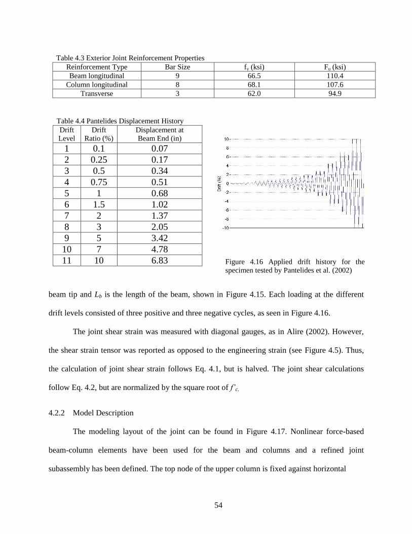
54

beam tip and Lb is the length of the beam, shown in Figure 4.15. Each loading at the different

drift levels consisted of three positive and three negative cycles, as seen in Figure 4.16.

The joint shear strain was measured with diagonal gauges, as in Alire (2002). However,

the shear strain tensor was reported as opposed to the engineering strain (see Figure 4.5). Thus,

the calculation of joint shear strain follows Eq. 4.1, but is halved. The joint shear calculations

follow Eq. 4.2, but are normalized by the square root of f’c.

4.2.2 Model Description

The modeling layout of the joint can be found in Figure 4.17. Nonlinear force-based

beam-column elements have been used for the beam and columns and a refined joint

subassembly has been defined. The top node of the upper column is fixed against horizontal

Table 4.3 Exterior Joint Reinforcement Properties

Reinforcement Type Bar Size fy (ksi) Fu (ksi)

Beam longitudinal 9 66.5 110.4

Column longitudinal 8 68.1 107.6

Transverse 3 62.0 94.9

Table 4.4 Pantelides Displacement History

Drift

Level Drift

Ratio (%) Displacement at

Beam End (in)

1 0.1 0.07

2 0.25 0.17

3 0.5 0.34

4 0.75 0.51

5 1 0.68

6 1.5 1.02

7 2 1.37

8 3 2.05

9 5 3.42

10 7 4.78

11 10 6.83 Figure 4.16 Applied drift history for the

specimen tested by Pantelides et al. (2002)

55

translation and a vertical load is applied to represent the compressive column axial load. The

bottom node of the lower column is pinned and the vertical reaction at this node will be used to

find the lateral load on the system. The lateral displacement will be applied at the right node of

the beam, which will be otherwise free to rotate or translate. The fixity and loading conditions

have been detailed in Figure 4.17a.

Figure 4.17b and c detail the model layout of the joint subassembly. All elements are

nonlinear truss elements except for the beam and column interface elements, which are rigid

beam-columns. The cross-sectional areas of the truss elements can be found in Figure 4.17b. A 4

cell by 4 cell joint core mesh has been selected, giving vertical and horizontal truss element

Full model layout

a) Joint element labels by area

b) Joint element labels by material type

Figure 4.17 Exterior joint model layout

56

lengths of 3.25” and an incline angle of 45°. Column longitudinal, beam longitudinal, and

transverse steel elements are given No. 8, No. 9, and No. 3 steel reinforcement properties,

respectively. Differing material properties are ascribed to the horizontal and diagonal concrete

elements to represent given confining pressures, whereas the material properties are ascribed

similarly for all vertical concrete elements. Bond-slip is modeled with zero-length springs and

the properties are dependent on location, type, and surface area of reinforcing bars.

4.2.3 Discussion of Results

Comparison of the lateral load-drift responses of the experimental results and the

simulated results can be found in Figure 4.18. The model presents good agreement with the

initial stiffness and peak strength of the measured data. The first yield of longitudinal

reinforcement in the model coincides with the first measured yield in longitudinal reinforcement

in the specimen. The onset of diagonal concrete crushing in the compression strut of the model,

illustrated in Figure 4.20, also coincides with the formation of the joint shear mechanism in the

specimen, pictured in Figure 4.19. Though the specimen degradation pattern is not well captured

in the cyclic simulation, the onset of significant concrete spalling in the specimen is well

approximated by the degradation of the monotonic curve, as seen in Figure 4.18.

A comparison of the normalized joint shear stress-joint shear strain of the measured

response and of the joint model, as seen in Figure 4.21, shows a good prediction of the peak

strength. The initial tangent modulus is slightly more steep in the measured response as

compared with the simulated response, however the simulation has a steeper tangent modulus in

the post-peak portion of the response compared with the envelope of the measured response. The

crushing of concrete along the primary compression strut within the model leads to a rapid loss

of shear strength and large shear deformations within the joint.

57

Figure 4.18 Lateral load-drift responses for the exterior joint

Figure 4.19 Observed cracking pattern at

formation of joint shear mechanism.

Pantelides, C., Hansen, J., Nadauld, J., and

Reaveley, L. (2002), “Assessment of

Reinforced Concrete Building Exterior Joints

with Substandard Details.” Report No. PEER-

2002/18, Berkeley, CA. Photo used under fair

use, 2014.

Figure 4.20 Simulated crack pattern at first

concrete crushing

58

4.3 Effects of Key Model Assumptions

The effects of bond-slip and joint confinement on the initial stiffness, peak strength, and

ductility of the modeling scheme were investigated in this study. Bond-slip was modeled with

zero-length elements at all nodes where longitudinal steel elements came into contact with

concrete elements. The constitutive model developed by Mitra and Lowes (2007) was utilized for

this study. Confinement parameters as a function of column axial load were calculated based on

the expressions of Mander et al. (1988). The column axial load provided the confining pressure

for the horizontal and diagonal elements within the columns and the joint. No confining effect

was considered for vertical elements or for elements within the beams.

As can be seen in Figure 4.22, bond-slip had a positive effect on all specimens. It had

very little effect on initial stiffness, but in all specimens it improved ductility. This is likely due

to the steel elements’ ability to undergo greater yielding without causing excessive deformation

Concrete

spalling in

specimen

Figure 4.21 Normalized joint shear stress-joint shear strain responses for the exterior joint

59

in the concrete elements. In the second interior joint and the exterior joint, pictured in Figure

4.22b and c, it also improved the approximation of peak strength.

The concrete confinement due to axial column load also had a clear positive effect on the

exterior joint, as is evident in Figure 4.23c. The strength has significantly improved, with the

simulated peak positive strength coming to within 1.5% of the measured peak strength, both

a) First interior joint b) Second interior joint

c) Exterior joint

Figure 4.22 Comparison of experimental lateral load-drift response to simulated lateral load-drift responses

with and without bond-slip effect

60

a) First interior joint b) Second interior joint

c) Exterior joint

Figure 4.23 Comparison of experimental lateral load-drift response to simulated lateral load-drift responses

with and without confinement effect

occurring at the same interstory drift. The degradation curve was also improved, leading to a less

sharp decline after the crushing of joint core concrete. The simulated response of the first interior

joint was also positively in terms of ductility approximations, as seen in Figure 4.23a. For the

second interior joint, the confinement lead to an over prediction of system ductility because of

the increased concrete strength, as is evident in Figure 4.23b.

61

Chapter 5. Conclusions and Recommendations for Future Research

This thesis has described a nonlinear truss modeling approach for non-ductile beam-to-

column joints, for which strength degradation occurs due to diagonal cracks. Concrete and steel

have been represented by truss elements that formed a lattice structure. Diagonal concrete

elements have accounted for the transverse strain effect in compression members, having

reduced compressive strength depending on the orthogonal tensile strain. An accurate steel

constitutive model has been implemented that accounts for distinct elastic, yield plateau, and

strain hardening regions, as well as having accurately represented the Bauschinger effect in

unloading. The reinforcing bar bond-slip relationship has been represented using zero-length

springs to connect concrete and steel elements. The model has been verified by comparing the

simulated responses to the experimentally measured responses of three poorly detailed beam-to-

column joints: two interior joints and one exterior joint.

5.1 Conclusions

1. The proposed model has predicted well the cyclic response of beam-to-column

connections with shear-dominated failures, especially in terms of the initial stiffness

and strength in the direction of first loading. The model has overestimated the

stiffness and strength in the negative loading direction compared with the

experimentally measured results, having given strengths in the negative loading

direction that are up to 24% higher than the measured values.

2. The onset of longitudinal beam steel yielding and diagonal compression strut

crushing, as well as the crack pattern formation, have been well predicted by the

model. The onset of these events has typically occurred within the same loading cycle

in both the experimental tests and the simulations.

62

3. The strength and ductility of the joint have been better captured by including bond-

slip in the modeling scheme.

4. The confining pressures of the diagonal and horizontal concrete elements have been

well predicted by the vertical pressure due to the column axial load. However, this

confining effect has lead to an over prediction of joint ductility.

5.2 Recommendations for Future Research

Future research should include an investigation into the strength and stiffness of the

negative loading direction. The formation of cracks during the first positive loading may have an

effect on the strength in this negative loading direction.

Degradation in the model occurs very swiftly after the first crushing of a concrete

element within the diagonal compression strut. Redundancy to account for this and allow for the

greater ductility typically seen in beam-to-column joints should be investigated further.

Accounting for dowel action in the reinforcing bars is one suggested approach.

A further refinement of the calculations to determine the confinement of the concrete due

to column axial load is suggested. The dependence of confinement on joint concrete spalling and

bar buckling is a possible source of variability. A broader range of column axial load levels,

including tensile axial loads caused by overturning of the moment frame, should be investigated.

Further research should be conducted to broaden the applicability of the model. Of

particular interest would be an investigation into the applicability of the model to well-detailed,

modern joints which rely more heavily on the panel-truss shear mechanism. A variety of failure

types should also be studied.

A comparison of the modeling scheme to refined finite element models should be made,

particularly looking at accuracy and computational efficiency.

63

References

ACI (1971), Building Code Requirements for Structural Concrete, ACI 318-71, American

Concrete Institute.

ACI (1985), Recommendations for Design of Beam-Column Connections in Monolithic

Reinforced Concrete Structures, ACI 352-85, American Concrete Institute.

Alath, S., and Kunnath, S. (1995), “Modeling Inelastic Shear Deformation in RC Beam-Column

Joints.” Proceedings of the 10th

Engineering Mechanics Conference, Boulder, CO, 822-

825

Alire, D. (2002), “Seismic Evaluation of Existing Unconfined Reinforced Concrete Beam-

Column Joints.” M.S. Thesis, University of Washington, Seattle, WA, 306pp.

Anderson, M., Lehman, D., and Stanton, J. (2008), “A cyclic shear stress-strain model for joints

without transverse reinforcement.” Engineering Structures 30, 941-954

Baglin, R. H., and Scott, P. S. (2000), “Finite Element Modeling of Reinforced Concrete Beam-

Column Connections.” ACI Structural Journal 97(6), 886-894

Beres, A., Pessiki, S., White, R., and Gergely, P. (1991), “Seismic performance of existing

reinforced concrete frames designed primarily for gravity loads.” Proceedings of the 6th

Canadian Conf. Earthquake Engineering, Toronto, Canada, 655-662

Beres, A., White, R., Gergely, P., Pessiki, S., and El-Atta, A. (1992), “Behavior of existing non-

seismically detailed reinforced concrete frames.” Proceedings of the 10th

Earthquake

Engineering World Conference, Balkema, Rotterdam, 3359-3363

Beres, A., Pessiki, S., White, R., and Gergely, P. (1996), “Implications of Experiments on the

Seismic Behavior of Gravity Load Designed RC Beam-to-Column Connections.”

Earthquake Spectra 12(2), 185-198

Biddah, A., and Ghobarah, P. (1999), “Modelling of Shear Deformation and Bond Slip in

Reinforced Concrete Joints.” Structural Engineering and Mechanics 7(4), 413-432

Birely, A., Lowes, L., and Lehman, D. (2011), “A model for the practical nonlinear analysis of

reinforced-concrete frames including joint flexibility.” Engineering Structures 34, 455-

465

Ciampi, V., Eligehausen, R., Bertero, V., and Popov, E. (1981), “Analytical Model for Deformed

Bar Bond under Generalized Excitations.” Proceedings of the IABSE Colloquium on

Advanced Mechanics of Reinforced Concrete, Delft, Netherlands

Comartin, C., Anagnos, T., Faison, H., Greene, M., and Moehle, J. (2008), “The Concrete

Coalition: Building a Network to Address Nonductile Concrete Buildings.” Proceedings

of the 14th

World Conference on Earthquake Engineering, Beijing, China

Dodd, L., and Restrepo-Posada, J. (1995), “Model for Predicting Cyclic Behavior of Reinforcing

Steel.” Journal of Structural Engineering 121(3), 433-445

Durrani, A., and Zerbe, H. (1987), “Seismic Resistance of R/C Exterior Connections with Floor

Slabs.” Journal of Structural Engineering 113(8), 1850-1864

Ehsani, M., and Wight, J. (1985), “Exterior Reinforced Concrete Beam-to-Column Connections

Subjected to Earthquake- Type Loading.” ACI Journal 82-43, 492-499

Eligehausen, R., Popov, E., and Bertero, V. (1983), “Local Bond Stress-Slip Relationships of

Deformed Bars Under Generalized Excitations.” Report No. UCB/EERC-83/23,

Berkeley, CA.

Filippou, F., Popov, E., and Bertero, V. (1983), “Modeling of R/C Joints under Cyclic

Excitations.” Journal of Structural Engineering 109(11), 2666-2684

64

Filson, J. R., McCarthy, J., Ellsworth, W. L., and Zoback, M. L. (2003), “The USGS earthquake

hazards program in NEHRP—Investing in a safer future.” USGS Fact Sheet 017-03,

Reston, VA.

Hassan, W. M., Park, S., Lopez, R. R., Mosalam, K. M., and Moehle, J. P. (2010), “Seismic

Response of Older-Type Reinforced Concrete Corner Joints.” Proceedings of the 9th

U.S.

National and 10th

Canadian Conference on Earthquake Engineering, Toronto, Ontario,

Canada, Paper No. 1616

Kashiwazaki, T., Nagai, T., and Noguchi, H. (1996), “Parametric Study on the Shear Strength of

RC Interior Beam-Column Joints Using Finite Element Method.” Transactions of the

Japan Concrete Institute 18, 275-282

Kim, J., and LaFave, J. (2006), "Key influence parameters for the joint shear behaviour of

reinforced concrete (RC) beam-column connections." Engineering Structures 29, 2523-

2539

Leon, R. (1989), “Interior Joints with Variable Anchorage Lengths.” Journal of Structural

Engineering 115(9), 2261-2275

Leon, R. (1990), “Shear Strength and Hysteretic Behavior of Interior Beam-Column Joints.” ACI

Structural Journal 87(1), 3-11

Leon, R., Kam, W., and Pampanin, S. (2014), “Performance of Beam-Column Joints in the 2010-

2012 Christchurch Earthquakes.”ACI SP-296-3

Lowes, L., (1999), “Finite element modeling of reinforced concrete beam-column bridge

connections.” Ph.D. Dissertation, Univ. of California, Berkeley, CA

Lowes, L., and Altoontash, A. (2003), “Modeling Reinforced-Concrete Beam-Column Joints

Subjected to Cyclic Loading.” Journal of Structural Engineering 129(12), 1686-1697

Lowes, L., Mitra, N., and Altoontash, A. (2004), “A Beam-Column Joint Model for Simulating

the Earthquake Response of Reinforced Concrete Frames.” Report No. PEER-2003/10,

Berkeley, CA.

Lu, Y., and Panagiotou, M. (2013), “Three-Dimensional Cyclic Beam-Truss Model for Non-

Planar Reinforced Concrete Walls.” Journal of Structural Engineering, accepted

manuscript

Mander, J. B., Priestley, M. J. N., and Park, R., (1988), “Theoretical Stress-Strain Model for

Confined Concrete.” Journal of Structural Engineering 114(8), 1804-1826

McKenna, F., et al. (2005). “OpenSees: Open system for earthquake engineering simulation.”

http://opensees.berkeley.edu, University of California, Berkeley.

Mitra, N., and Lowes, L. (2007), “Evaluation, Calibration, and Verification of a Reinforced

Concrete Beam-Column Joint Model.” Journal of Structural Engineering 133(1), 105-

120

Mosier, W. G. (2000), “Seismic Assessment of Reinforced Concrete Beam-Column Joints.” M.S.

Thesis, University of Washington, Seattle, WA, 218 pp.

Noguchi, H. (1981), “Nonlinear Finite Elements Analysis of Reinforced Concrete Beam-Column

Joints.” Reports of the Working Commissions (International Association for Bridge and

Structural Engineering 34, 639-654

Pagni, C., and Lowes, L. (2004), “Predicting Earthquake Damage in Older Reinforced Concrete

Beam-Column Joints.” Report No. PEER-2003/17, Berkeley, CA

Pampanin, S., Magenes, G., and Carr, A. (2003), “Modeling of Shear Hinge Mechanism in

Poorly Detailed RC Beam-Column Joints.” FIB Symposium, Concrete Structures in

Seismic Regions, Athens, Greece

65

Panagiotou, M., and Restrepo, J. I. (2011), “Nonlinear Cyclic Truss Model for Strength

Degrading Plane Stress Reinforced Concrete Elements.” Report No. UCB/SEMM-

2011/01, Berkeley, CA.

Panagiotou, M., Restrepo, J. I., Schoettler, M., and Kim, G. (2012), “Nonlinear Cyclic Truss

Model for Reinforced Concrete Walls.” ACI Structural Journal 109(2), 205-214

Pantazopoulou, S. J., and Bonacci, J. F. (1994), “On earthquake-resistant reinforced concrete

frame connections.” Canadian Journal of Civil Engineering 21, 307-328

Pantelides, C., Hansen, J., Nadauld, J., and Reaveley, L. (2002), “Assessment of Reinforced

Concrete Building Exterior Joints with Substandard Details.” Report No. PEER-2002/18,

Berkeley, CA

Park, S., and Mosalam, K. (2009), “Shear Strength Models of Exterior Beam-Column Joints

without Transverse Reinforcement.” Report No. Peer-2009/106, Berkeley, CA

Paulay, T., Park, R., and Priestley, M. J. N. (1978), “Reinforced Concrete Beam-Column Joints

Under Seismic Actions.” Journal of the American Concrete Institute 75(11), 585-593

Paulay, T., and Scarpas, A. (1981), “The Behavior of Exterior Beam-Column Joints.” Bulletin of

the New Zealand National Society for Earthquake Engineering 14(3), 131-144

Raynor, D. J. (2000), “Bond Assessment of Hybrid Frame Continuity Reinforcement.” M.S.

Thesis, University of Washington, Seattle, WA, 248 pp.

Restrepo-Posada, J. I., Dodd, L. L., and Cooke, N. (1994), “Variables Affecting Cyclic Behavior

of Reinforcing Steel.” Journal of Structural Engineering 120(11), 3178-3196

Sezen, H., Elwood, K. J., Whittaker, A. S., Mosalam, K. M., Walace, J. W., and Stanton, J. F.,

(2000), “Sezen - Structural Engineering Reconnaissance of the August 17, 1999, Kocaeli

(Izmit), Turkey, Earthquake.” Report No. PEER-2000/09, Berkeley, CA

Sharma, A., Eligehausen, R., and Reddy, G. (2011), “A new model to simulate joint shear

behavior of poorly detailed beam-column connection in RC structures under seismic

loads, Part I: Exterior joints.” Engineering Structures 33, 1034-1051

Shin, M., and LaFave, J. (2004), “Testing and Modeling for Cyclic Joint Shear Deformations in

RC Beam-Column Connections.” Proceedings of the 13th

World Conference on

Earthquake Engineering, Vancouver, Canada

Vecchio, F., and Collins, M. (1986), “The modified compression field theory for reinforced

concrete elements subjected to shear.” Journal of the American Concrete Institute 83(2),

219-231

66

Appendix A. DoddRestr Steel Constitutive Model Source Code

function hr = Doddrestr(e_s,hr,d) % Function to define stress-strain behavior of steel under cyclic loading. % List of variables % ep_a = natural strain at initiation of Bauschinger effect % ep_M = maximum plastic strain defined as greater of |ep_o(1)| or ep_o(2) % epp_N = transformed-normalized natural strain % ep_o(k) = "shifted" origin strain (k = 1 for compression, 2 for tension) % ep_p = strain magnitude between inclined envelope and point at initiaion % of Bauschinger effect in natural coordinate system % ep_r(m) = natural strain at reversal point (m = 1 for max tension, m = 2 % for max compression) % e_s = steel strain in engineering coordinate system % ep_s = steel strain in natural coordinate system % ep_sh = natural strain at initiation of work hardening % ep_sh1 = arbitrary natural strain in work hardening region of tension % monotonic curve % ep_su = "ultimate" strain in natural coordinate system % ep_sushift(k) = natural strain associated with "ultimate" true stress % Ep_u = natural coordinate unload modulus % Em_s = initial elastic modulus % fp_a = true stress at initiation of Bauschinger effect % fp_p = stress magnitude between inclined envelope and point at initiation % of Bauschinger effect in natural coordinate system % fp_r(m) = true stress at reversal point (m = 1 for max tension, m = 2 % for max compression) % f_s = engineering stress of steel % fp_s = true stress of steel % fp_sh = true stress at onset of strain hardening % fp_sh1 = true stress at arbitrary point ep_sh1 % fp_su = "ultimate stress" in natural coordinates % fps_su = slope at "ultimate stress" in natural coordinates, numerically % equal to fo_su % fp_t = stress magnitude between top and bottom inclined envelopes in % natural coordinate system % f_y = yield stress of steel in engineering coordinate system % load = loading direction (1 for compression, 2 for tension) % P = exponential factor to define work hardening region of skeleton curve % and shape of Bauschinger effect % region = region of model % region = 0: We load along the skeleton curve, we do not store any % unloading-reloading points % region = 1: Major reversal, (s1 = -1) % region = 2: Major reversal, (s1 = 1) % region = 3: Minor reversal, "minor point" on positive side (s1 = -1) % region = 4: Minor reversal, "minor point" on negative side (s1 = 1) % region = 5: Simple reversal, s1 = -1,inside a "region3" % region = 6: Simple reversal, s1 = -1,inside a "region4" % region = 7: Simple reversal, s1 = 1,inside a "region3" % region = 8: Simple reversal, s1 = 1,inside a "region4" % point: array with dimension (6x3), row = point number % column: 1 = strain, 2 = stress, 3 = slope % row: 1=largest tensile major reversal or farthest tensile point % 2=largest compressive major reversal or farthest % compressive point

67

% 3=immediate tensile reconnect point % 4=immediate compressive reconnect point % 5=last tensile reversal % 6=last compressive reversal

% s1 = strain direction factor (1 for tension, -1 for compression) % virgin = 1 for virgin loading, 0 for non-virgin % W = (omega) partial area under normalized Bauschinger curve

% ----------------------------------------------------------------------- % ----------------------------------------------------------------------- % Reading history variables e_so = hr(1); f_so = hr(2); yield1 = hr(3); region = hr(4); point(1,1) = hr(5); point(1,2) = hr(6); point(1,3) = hr(7); point(2,1) = hr(8); point(2,2) = hr(9); point(2,3) = hr(10); point(3,1) = hr(11); point(3,2) = hr(12); point(3,3) = hr(13); point(4,1) = hr(14); point(4,2) = hr(15); point(4,3) = hr(16); point(5,1) = hr(17); point(5,2) = hr(18); point(5,3) = hr(19); ep_o(1) = hr(20); ep_o(2) = hr(21); ep_M = hr(22); fps_so = hr(23); hist1(1) = hr(24); hist1(2) = hr(25); point(6,1) = hr(26); point(6,2) = hr(27); point(6,3) = hr(28); sim1 = hr(29); stiff = hr(30);

% Reading material properties Em_s = d(1); f_y = d(2); e_sh = d(3); e_sh1 = d(4); f_sh1 = d(5); e_su = d(6); f_su = d(7); P_major = d(8); P_minor = d(9);

% Converting from engineering strain to true strain ep_sh = log(1+e_sh);

68

fp_sh = f_y*exp(ep_sh); ep_sh1 = log(1+e_sh1); fp_sh1 = f_sh1*exp(ep_sh1); ep_su = log(1+e_su); fp_su = f_su*exp(ep_su); fps_su = exp(ep_su)*f_su; ep_s = log(1+e_s); ep_so = log(1+e_so); fp_so = f_so*(1+e_so);

% Calculate Ep_u (unloading-Reloading modulus) if (yield1 > 0.5) Ep_u = Em_s*(0.82+1/(5.55+1000*ep_M)); else Ep_u = Em_s; end

% Calculate shifted ultimate strain ep_sushift(1) = ep_su+ep_o(1); ep_sushift(2) = -ep_su+ep_o(2);

% Give positive value if you want to set a constant P = P_major, % otherwise use Eq 36 (Dodd and Restrepo, 1995) to solve for P if (P_major > 0) icheat = 1; else icheat = 0; end

if((ep_s >= point(1,1)) || (ep_s <= point(2,1))... || ep_s >= ep_sushift(1) || ep_s <= ep_sushift(2)) if(ep_s >= point(1,1) || (ep_s) >= ep_sushift(1)) %if in tension ep_o1 = ep_o(1); if(hist1(1) > 0.5) s1 = 1; k = 1; ep_a = point(2,1)+s1*f_y/Ep_u; fp_a = point(2,2)+s1*f_y; ep_sushift(k) = s1*ep_su+ep_o(k); ep_rejoin = ep_sushift(k); fp_rejoin = s1*fp_su; fps_rejoin = fps_su; if(ep_s >= ep_sushift(k)) fp_s = s1*fp_su; fps_s = fps_su; ep_sushift(k) = ep_s; ep_o(k) = ep_sushift(k)-s1*ep_su; else [fp_s,fps_s] = Bauschinger(1,icheat,P_major,P_minor,... ep_sushift,s1,fp_su,Ep_u,ep_a,fp_a,ep_s,k,... ep_rejoin,fp_rejoin,fps_rejoin,ep_o,ep_so,fp_so); end else [fp_s,fps_s] = virginLoading; end else %if in compression

69

ep_o1 = ep_o(2); if(hist1(2) > 0.5) s1 = -1; k = 2; ep_a = point(1,1)+s1*f_y/Ep_u; fp_a = point(1,2)+s1*f_y; ep_sushift(k) = s1*ep_su+ep_o(k); ep_rejoin = ep_sushift(k); fp_rejoin = s1*fp_su; fps_rejoin = fps_su; if(ep_s <= ep_sushift(k)) fp_s = s1*fp_su; fps_s = fps_su; else [fp_s,fps_s] = Bauschinger(1,icheat,P_major,P_minor,... ep_sushift,s1,fp_su,Ep_u,ep_a,fp_a,ep_s,k,... ep_rejoin,fp_rejoin,fps_rejoin,ep_o,ep_so,fp_so); end else [fp_s,fps_s] = virginLoading; end end

region = 0; %say we are not in a reversal point(3,1) = 0; %and erase all of the old reversal stuff point(3,2) = 0; point(3,3) = 0; point(4,1) = 0; point(4,2) = 0; point(4,3) = 0; point(5,1) = 0; point(5,2) = 0; point(5,3) = 0;

if(ep_s > point(1,1) || ep_s >= ep_sushift(1)) point(1,1) = ep_s; %if past the max previous tensile point/max point(1,2) = fp_s; %tensile reversal replace point 1 point(1,3) = fps_s; end

if(ep_s < point(2,1) || ep_s <= ep_sushift(2)) point(2,1) = ep_s; %if past the max previous compressive point/max point(2,2) = fp_s; %compressive reversal, replace point 2 point(2,3) = fps_s; end elseif(ep_s < point(1,1) && ep_s > point(2,1)) %--------------------------------------------------------------------- if(region < 0.5) %Reversal from virgin loading if(yield1 < 0.5)%Reversal in elastic branch fp_s = Em_s*ep_s; fps_s = Em_s; %check if greater than previous greatest points if(ep_s > point(1,1)) point(1,1) = ep_s; point(1,2) = fp_s; point(1,3) = fps_s;

70

end

if(ep_s < point(2,1)) point(2,1) = ep_s; point(2,2) = fp_s; point(2,3) = fps_s; end elseif(yield1 < 1.5) %Reversal in yield plateau if(ep_so < point(1,1) && ep_so > point(2,1)) if(point(5,2) > 0) %if it was a tensile reversal s1 = -1; k = 2; m = 1; region = 1; else %if it was a compressive reversal s1 = 1; k = 1; m = 2; region = 2; end else %if beyond point of last greatest reversal/max point reached point(5,1) = ep_so; point(5,2) = fp_so; point(5,3) = fps_so; if(fp_so > 0) s1 = -1; k = 2; m = 1; region = 1; else s1 = 1; k = 1; m = 2; region = 2; end end

ep_r = point(5,1); fp_r = point(5,2); fp_rejoin = s1*f_y; ep_rejoin = point(m,1)+s1*(ep_o(2)-ep_o(1)+2*f_y/Ep_u); fps_rejoin = f_y;

if(s1 < 0)%if we have yielded in tension and now unloading define %the "rejoin point" as the minimum attained strain point(2,1) = ep_rejoin; point(2,2) = fp_rejoin; point(2,3) = f_y; else %if we have yielded in compression and now unloading %define the "rejoin point" as the maximum attained strain point(1,1) = ep_rejoin; point(1,2) = fp_rejoin; point(1,3) = f_y; end

ep_sushift(k) = s1*ep_su+ep_o(k);

71

ep_a = ep_r+s1*f_y/Ep_u; fp_a = fp_r+s1*f_y;

if(abs(ep_s-ep_r) <= abs(ep_a-ep_r)) %if w/in linear portion fp_s = fp_r+Ep_u*(ep_s-ep_r); fps_s = Ep_u; else [fp_s,fps_s] = Bauschinger(0,icheat,P_major,P_minor,... ep_sushift,s1,fp_su,Ep_u,ep_a,fp_a,ep_s,k,... ep_rejoin,fp_rejoin,fps_rejoin,ep_o,ep_so,fp_so); end

%checking if beyond greatest previous reversal if(ep_s > point(1,1)) point(1,1) = ep_s; point(1,2) = fp_s; point(1,3) = fps_s; end

if(ep_s < point(2,1)) point(2,1) = ep_s; point(2,2) = fp_s; point(2,3) = fps_s; end

elseif(yield1 > 1.5) % ****** if WE HAVE ENTERED THE STRAIN HARDENING region point(5,1) = ep_so; point(5,2) = fp_so; point(5,3) = fps_so;

if(ep_s < ep_so) %if in compressive loading s1 = -1; k = 2; region = 1; hist1(2) = 1; point(1,1) = ep_so; point(1,2) = fp_so; point(1,3) = fps_so; else %if in tensile loading s1 = 1; k = 1; region = 2; hist1(1) = 1; point(2,1) = ep_so; point(2,2) = fp_so; point(2,3) = fps_so; end

ep_r = ep_so; fp_r = fp_so; ep_o(k) = ep_r+s1*fp_r/Ep_u; ep_sushift(k) = s1*ep_su+ep_o(k); ep_a = ep_r+s1*f_y/Ep_u; fp_a = fp_r+s1*f_y; ep_rejoin = ep_sushift(k);

72

fp_rejoin = s1*fp_su; fps_rejoin = fps_su;

if(abs(ep_s-ep_r) <= abs(ep_a-ep_r)) %if within linear portion fp_s = fp_r+Ep_u*(ep_s-ep_r); %of reversal fps_s = Ep_u; else [fp_s,fps_s] = Bauschinger(1,icheat,P_major,P_minor,... ep_sushift,s1,fp_su,Ep_u,ep_a,fp_a,ep_s,k,... ep_rejoin,fp_rejoin,fps_rejoin,ep_o,ep_so,fp_so); end end else %reversal from a reversal %----------------------------------------------------------------- if(region == 1)%Major compressive reversal (unloading in negative [fp_s,fps_s] = reverse1; %direction) %------------------------------------------------------------- elseif(region == 2)%Major tensile reversal (unloading in positive [fp_s,fps_s] = reverse2; %direction) %------------------------------------------------------------- elseif(region == 3) %Minor compressive reversal (unloading in %negative direction) if(ep_s > point(5,1) && ep_s <= point(1,1))%if back to major point(5,1) = point(2,1); %reversal from which point(5,2) = point(2,2); %we left and not to point(5,3) = point(2,3); %skeleton curve point(4,1) = 0; point(4,2) = 0; point(4,3) = 0; region = 2; [fp_s,fps_s] = reverse2; else %if still in minor reversal (or back to skeleton curve) [fp_s,fps_s] = reverse3; end %------------------------------------------------------------- elseif(region == 4) %Minor tensile reversal (unloading in %positive direction) if(ep_s < point(5,1) && ep_s >= point(2,1))%if back to major point(5,1) = point(1,1); %reversal from which point(5,2) = point(1,2); %we left and not to point(5,3) = point(1,3); %skeleton curve point(4,1) = 0; point(4,2) = 0; point(4,3) = 0; region = 1; [fp_s,fps_s] = reverse1; else %if still in minor reversal [fp_s,fps_s] = reverse4; end %------------------------------------------------------------- elseif(region == 5) %simple reversal unloading in negative direction %within region 3 (region 3 = minor unloading in %negative direction) if(ep_s > point(4,1) && ep_s <= point(1,1)) %if we have reversed point(5,1) = point(2,1); %and are now within point(5,2) = point(2,2); %the major reversal point(5,3) = point(2,3); %from which we came

73

point(4,1) = 0; point(4,2) = 0; point(4,3) = 0; region = 2; sim1 = 0; [fp_s,fps_s] = reverse2; else [fp_s,fps_s] = reverse5; end %------------------------------------------------------------- elseif(region == 6) %simple reversal unloading in negative direction %within region 4 (region 4 = minor unloading in %positive direction) if(ep_s < point(4,1) && ep_s >= point(2,1)) %if back to w/in the point(5,1) = point(1,1); %major reversal from point(5,2) = point(1,2); %which we came point(5,3) = point(1,3); point(4,1) = 0; point(4,2) = 0; point(4,3) = 0; region = 1; sim1 = 0; [fp_s,fps_s] = reverse1; elseif((ep_s > point(5,1) && ep_s < point(1,1)) && sim1 < 0.5) point(5,1) = point(4,1); %if we have reversed and are back to point(5,2) = point(4,2); %aiming for the major compressive point(5,3) = point(4,3); %reversal point region = 4; sim1 = 0; [fp_s,fps_s] = reverse4; else [fp_s,fps_s] = reverse6; end %------------------------------------------------------------- elseif(region == 7) %simple reversal unloading in positive direction %within region 3 (region 3 = minor unloading in %negative direction) if(ep_s > point(4,1) && ep_s <= point(1,1)) %if back to w/in the point(5,1) = point(2,1); %major reversal from point(5,2) = point(2,2); %which we came point(5,3) = point(2,3); point(4,1) = 0; point(4,2) = 0; point(4,3) = 0; region = 2; sim1 = 0; [fp_s,fps_s] = reverse2; elseif(ep_s < point(6,1) && ep_s > point(2,1) && sim1 < 0.5) point(5,1) = point(4,1); %if we have reversed and are back to point(5,2) = point(4,2); %aiming for the major compressive point(5,3) = point(4,3); %reversal point region = 3; sim1 = 0; [fp_s,fps_s] = reverse3; else [fp_s,fps_s] = reverse7; end

74

%------------------------------------------------------------- elseif(region == 8) %simple reversal unloading in positive direction %within region 4 (region 4 = minor unloading in %positive direction) if(ep_s < point(4,1) && ep_s >= point(2,1)) %if we have reversed point(5,1) = point(1,1); %and are now within point(5,2) = point(1,2); %the major reversal point(5,3) = point(1,3); %from which we came point(4,1) = 0; point(4,2) = 0; point(4,3) = 0; region = 1; sim1 = 0; [fp_s,fps_s] = reverse1; else [fp_s,fps_s] = reverse8; end end end end

%------------------------------------ % UPDATE HISTORY VARIABLES f_s = fp_s/exp(ep_s);

if stiff fs_s = fps_s*(1/(e_s+1))^2; else fs_s = Em_s; end

if(yield1 > 0.5 && ep_s < 0 && ep_s <= point(2,1)... && ((ep_s+0.002) < (-1*ep_M))) ep_M = abs(ep_s+0.002); end

if(yield1 > 0.5 && ep_s > 0 && ep_s >= point(1,1)... && ((ep_s-0.002) > ep_M)) ep_M = (ep_s-0.002); end

if(yield1 > 0.5) Ep_u = Em_s*(0.82+1./(5.55+1000.*ep_M)); else Ep_u = Em_s; end

if(yield1 > 0.5 && yield1 < 1.5 && region < 0.5) ep_o(2) = point(1,1)-point(1,2)/Ep_u; ep_o(1) = point(2,1)-point(2,2)/Ep_u; end

%Update history variables hr(1) = e_s; hr(2) = f_s;

75

hr(3) = yield1; hr(4) = region; hr(5) = point(1,1); hr(6) = point(1,2); hr(7) = point(1,3); hr(8) = point(2,1); hr(9) = point(2,2); hr(10) = point(2,3); hr(11) = point(3,1); hr(12) = point(3,2); hr(13) = point(3,3); hr(14) = point(4,1); hr(15) = point(4,2); hr(16) = point(4,3); hr(17) = point(5,1); hr(18) = point(5,2); hr(19) = point(5,3); hr(20) = ep_o(1); hr(21) = ep_o(2); hr(22) = ep_M; hr(23) = fps_s; hr(24) = hist1(1); hr(25) = hist1(2); hr(26) = point(6,1); hr(27) = point(6,2); hr(28) = point(6,3); hr(29) = sim1; hr(31) = fs_s;

% =======================================================================

function [fp_s,fps_s] = reverse1 f_y = d(2); e_su = d(6); f_su = d(7); P_major = d(8); P_minor = d(9); ep_su = log(1+e_su); fp_su = f_su*exp(ep_su); fps_su = exp(ep_su)*f_su; s1 = -1; k = 2; m = 1;

%*************************************************************************

if(yield1 < 1.5) if((ep_s-ep_so) <= 0.0) %We continue unloading ep_sushift(k) = s1*ep_su+ep_o(k); ep_a = point(5,1)+s1*f_y/Ep_u; fp_a = point(5,2)+s1*f_y;

if((point(5,1)-ep_s) <= (point(5,1)-ep_a)) fp_s = point(5,2)+Ep_u*(ep_s-point(5,1)); fps_s = Ep_u; else

76

fp_rejoin = s1*f_y; ep_rejoin = point(m,1)+s1*(ep_o(2)-ep_o(1)+2*f_y/Ep_u); fps_rejoin = f_y; [fp_s,fps_s] = Bauschinger(0,icheat,P_major,P_minor,... ep_sushift,s1,fp_su,Ep_u,ep_a,fp_a,ep_s,k,... ep_rejoin,fp_rejoin,fps_rejoin,ep_o,ep_so,fp_so); end else ep_a = point(5,1)+s1*f_y/Ep_u; fp_a = point(5,2)+s1*f_y; if(((point(5,1)-ep_so) <= (point(5,1)-ep_a)) &&... ((point(5,1)-ep_s) <= (point(5,1)-ep_a))) fp_s = point(5,2)+Ep_u*(ep_s-point(5,1)); fps_s = Ep_u; else %We have a MINOR reversal point(3,1) = point(5,1); point(3,2) = point(5,2); point(3,3) = point(5,3); point(4,1) = ep_so; point(4,2) = fp_so; point(4,3) = fps_so; point(5,1) = ep_so; point(5,2) = fp_so; point(5,3) = fps_so; region = 4; [fp_s,fps_s] = reverse4; end end

%*************************************************************************

else ep_a = point(5,1)+s1*f_y/Ep_u; fp_a = point(5,2)+s1*f_y; if(ep_s <= ep_so) ep_sushift(k) = s1*ep_su+ep_o(k); ep_a = point(5,1)+s1*f_y/Ep_u; fp_a = point(5,2)+s1*f_y; ep_rejoin = ep_sushift(k); fp_rejoin = s1*fp_su; fps_rejoin = fps_su; if((point(5,1)-ep_s) <= (point(5,1)-ep_a)) fp_s = point(5,2)+Ep_u*(ep_s-point(5,1)); fps_s = Ep_u; else [fp_s,fps_s] = Bauschinger(1,icheat,P_major,P_minor,... ep_sushift,s1,fp_su,Ep_u,ep_a,fp_a,ep_s,k,... ep_rejoin,fp_rejoin,fps_rejoin,ep_o,ep_so,fp_so); end else if(((point(5,1)-ep_so) <= (point(5,1)-ep_a)) && ... ((point(5,1)-ep_s) <= (point(5,1)-ep_a))) fp_s = point(5,2)+Ep_u*(ep_s-point(5,1)); fps_s = Ep_u; else if((point(5,2)-fp_so) >= 2*f_y) %We have a MAJOR reversal

77

point(5,1) = ep_so; point(5,2) = fp_so; point(5,3) = fps_so; point(2,1) = ep_so; point(2,2) = fp_so; point(2,3) = fps_so; region = 2; s1 = 1; k = 1; ep_o(k) = ep_so-s1*fp_so/Ep_u; ep_sushift(k) = s1*ep_su+ep_o(k); ep_o(1) = ep_so+fp_so/Ep_u; ep_sushift(1) = ep_o(1)+ep_su; if(hist1(1) < 0.5) hist1(1) = 1; end [fp_s,fps_s] = reverse2; else %We have a MINOR reversal region = 4; point(3,1) = point(5,1); point(3,2) = point(5,2); point(3,3) = point(5,3); point(4,1) = ep_so; point(4,2) = fp_so; point(4,3) = fps_so; point(5,1) = ep_so; point(5,2) = fp_so; point(5,3) = fps_so; [fp_s,fps_s] = reverse4; end end end end end

% =======================================================================

function [fp_s,fps_s] = reverse2 f_y = d(2); e_su = d(6); f_su = d(7); P_major = d(8); P_minor = d(9); ep_su = log(1+e_su); fp_su = f_su*exp(ep_su); fps_su = exp(ep_su)*f_su; s1 = 1; k = 1; m = 2;

%*************************************************************************

if(yield1 < 1.5) if(ep_s >= ep_so) % we continue unloading ep_sushift(k) = s1*ep_su+ep_o(k); ep_a = point(5,1)+s1*f_y/Ep_u;

78

fp_a = point(5,2)+s1*f_y;

if(((point(5,1)-ep_s) >= (point(5,1)-ep_a))) fp_s = point(5,2)+Ep_u*(ep_s-point(5,1)); fps_s = Ep_u; else fp_rejoin = s1*f_y; ep_rejoin = point(m,1)+s1*(ep_o(2)-ep_o(1)+2*f_y/Ep_u); fps_rejoin = f_y; [fp_s,fps_s] = Bauschinger(0,icheat,P_major,P_minor,... ep_sushift,s1,fp_su,Ep_u,ep_a,fp_a,ep_s,k,... ep_rejoin,fp_rejoin,fps_rejoin,ep_o,ep_so,fp_so); end else ep_a = point(5,1)+s1*f_y/Ep_u; fp_a = point(5,2)+s1*f_y;

if(((point(5,1)-ep_so) >= (point(5,1)-ep_a)) && ... ((point(5,1)-ep_s) >= (point(5,1)-ep_a))) fp_s = point(5,2)+Ep_u*(ep_s-point(5,1)); fps_s = Ep_u; else %We have a MINOR reversal point(3,1) = point(5,1); point(3,2) = point(5,2); point(3,3) = point(5,3); point(4,1) = ep_so; point(4,2) = fp_so; point(4,3) = fps_so; point(5,1) = ep_so; point(5,2) = fp_so; point(5,3) = fps_so; region = 3; [fp_s,fps_s] = reverse3; end end

%*************************************************************************

else ep_a = point(5,1)+s1*f_y/Ep_u; fp_a = point(5,2)+s1*f_y;

if(ep_s >= ep_so) ep_sushift(k) = s1*ep_su+ep_o(k); ep_a = point(5,1)+s1*f_y/Ep_u; fp_a = point(5,2)+s1*f_y; ep_rejoin = ep_sushift(k); fp_rejoin = s1*fp_su; fps_rejoin = fps_su; if(((point(5,1)-ep_s) >= (point(5,1)-ep_a))) fp_s = point(5,2)+Ep_u*(ep_s-point(5,1)); fps_s = Ep_u; else [fp_s,fps_s] = Bauschinger(1,icheat,P_major,P_minor,... ep_sushift,s1,fp_su,Ep_u,ep_a,fp_a,ep_s,k,... ep_rejoin,fp_rejoin,fps_rejoin,ep_o,ep_so,fp_so);

79

end else if(((point(5,1)-ep_so) >= (point(5,1)-ep_a)) && ... ((point(5,1)-ep_s) >= (point(5,1)-ep_a))) fp_s = point(5,2)+Ep_u*(ep_s-point(5,1)); fps_s = Ep_u; else if((fp_so-point(5,2)) >= 2*f_y) %We have a MAJOR reversal! point(5,1) = ep_so; point(5,2) = fp_so; point(5,3) = fps_so; point(1,1) = ep_so; point(1,2) = fp_so; point(1,3) = fps_so;

if(hist1(2) < 0.5) hist1(2) = 1; end

region = 1; s1 = -1; k = 2; ep_o(k) = ep_so+s1*fp_so/Ep_u; ep_sushift(k) = s1*ep_su+ep_o(k); [fp_s,fps_s] = reverse1; else %We have a MINOR reversal point(3,1) = point(5,1); point(3,2) = point(5,2); point(3,3) = point(5,3); point(4,1) = ep_so; point(4,2) = fp_so; point(4,3) = fps_so; point(5,1) = ep_so; point(5,2) = fp_so; point(5,3) = fps_so; region = 3; [fp_s,fps_s] = reverse3; end end end end end

% =======================================================================

function [fp_s,fps_s] = reverse3 f_y = d(2); e_su = d(6); f_su = d(7); P_major = d(8); P_minor = d(9); ep_su = log(1+e_su); fp_su = f_su*exp(ep_su); fps_su = exp(ep_su)*f_su; s1 = -1; k = 2;

80

m = 1;

%*************************************************************************

if(ep_s <= ep_so) ep_sushift(k) = s1*ep_su+ep_o(k); ep_a = point(5,1)+s1*f_y/Ep_u; fp_a = point(5,2)+s1*f_y; ep_rejoin = point(3,1); fp_rejoin = point(3,2); fps_rejoin = point(3,3); if(((point(5,1)-ep_s) <= (point(5,1)-ep_a))) fp_s = point(5,2)+Ep_u*(ep_s-point(5,1)); fps_s = Ep_u; else [fp_s,fps_s] = Bauschinger(0,icheat,P_major,P_minor,... ep_sushift,s1,fp_su,Ep_u,ep_a,fp_a,ep_s,k,... ep_rejoin,fp_rejoin,fps_rejoin,ep_o,ep_so,fp_so); end else ep_a = point(5,1)+s1*f_y/Ep_u; fp_a = point(5,2)+s1*f_y; if(((point(5,1)-ep_so) <= (point(5,1)-ep_a)) && ... ((point(5,1)-ep_s) <= (point(5,1)-ep_a))) fp_s = point(5,2)+Ep_u*(ep_s-point(5,1)); fps_s = Ep_u; else %We have a SIMPLE reversal point(4,1) = point(5,1); point(4,2) = point(5,2); point(4,3) = point(5,3); point(6,1) = ep_so; point(6,2) = fp_so; point(6,3) = fps_so; region = 7; [fp_s,fps_s] = reverse7; end end end

% ========================================================================

function [fp_s,fps_s] = reverse4 f_y = d(2); e_su = d(6); f_su = d(7); P_major = d(8); P_minor = d(9); ep_su = log(1+e_su); fp_su = f_su*exp(ep_su); fps_su = exp(ep_su)*f_su; s1 = 1; k = 1; m = 2;

%*************************************************************************

81

if(ep_s >= ep_so) ep_sushift(k) = s1*ep_su+ep_o(k); ep_a = point(5,1)+s1*f_y/Ep_u; fp_a = point(5,2)+s1*f_y; ep_rejoin = point(3,1); fp_rejoin = point(3,2); fps_rejoin = point(3,3); if(((point(5,1)-ep_s) >= (point(5,1)-ep_a))) fp_s = point(5,2)+Ep_u*(ep_s-point(5,1)); fps_s = Ep_u; else [fp_s,fps_s] = Bauschinger(0,icheat,P_major,P_minor,... ep_sushift,s1,fp_su,Ep_u,ep_a,fp_a,ep_s,k,... ep_rejoin,fp_rejoin,fps_rejoin,ep_o,ep_so,fp_so); end else ep_a = point(5,1)+s1*f_y/Ep_u; fp_a = point(5,2)+s1*f_y; if(((point(5,1)-ep_so) >= (point(5,1)-ep_a)) && ... ((point(5,1)-ep_s) >= (point(5,1)-ep_a))) fp_s = point(5,2)+Ep_u*(ep_s-point(5,1)); fps_s = Ep_u;

else %We have a SIMPLE reversal point(4,1) = point(5,1); point(4,2) = point(5,2); point(4,3) = point(5,3); point(5,1) = ep_so; point(5,2) = fp_so; point(5,3) = fps_so; region = 6; [fp_s,fps_s] = reverse6; end end end

% ========================================================================

function [fp_s,fps_s] = reverse5 f_y = d(2); e_su = d(6); f_su = d(7); P_major = d(8); P_minor = d(9); ep_su = log(1+e_su); fp_su = f_su*exp(ep_su); fps_su = exp(ep_su)*f_su; s1 = -1; k = 2; m = 1;

%*************************************************************************

if(ep_s <= ep_so) ep_sushift(k) = s1*ep_su+ep_o(k); ep_a = point(5,1)+s1*f_y/Ep_u;

82

fp_a = point(5,2)+s1*f_y; ep_rejoin = point(3,1); fp_rejoin = point(3,2); fps_rejoin = point(3,3); if((point(5,1)-ep_s) <= (point(5,1)-ep_a)) fp_s = point(5,2)+Ep_u*(ep_s-point(5,1)); fps_s = Ep_u; else if(sim1 > 0.5) sim1 = 0; point(6,1) = 0; point(6,2) = 0; point(6,3) = 0; end [fp_s,fps_s] = Bauschinger(0,icheat,P_major,P_minor,... ep_sushift,s1,fp_su,Ep_u,ep_a,fp_a,ep_s,k,... ep_rejoin,fp_rejoin,fps_rejoin,ep_o,ep_so,fp_so); end else ep_a = point(5,1)+s1*f_y/Ep_u; fp_a = point(5,2)+s1*f_y; if(((point(5,1)-ep_so) <= (point(5,1)-ep_a)) && ... ((point(5,1)-ep_s) <= (point(5,1)-ep_a)) && ... (point(5,1) >= ep_s)) fp_s = point(5,2)+Ep_u*(ep_s-point(5,1)); fps_s = Ep_u; else %We have a new SIMPLE reversal if(sim1 < 0.5) point(6,1) = ep_so; point(6,2) = fp_so; point(6,3) = fps_so; sim1 = 1; else point(5,1) = 0; point(5,2) = 0; point(5,3) = 0; sim1 = 0; end

region = 7; [fp_s,fps_s] = reverse7; end end end

% ========================================================================

function [fp_s,fps_s] = reverse6 f_y = d(2); e_su = d(6); f_su = d(7); P_major = d(8); P_minor = d(9); ep_su = log(1+e_su); fp_su = f_su*exp(ep_su); fps_su = exp(ep_su)*f_su;

83

s1 = -1; k = 2; m = 1;

%*************************************************************************

if(ep_s <= ep_so) ep_sushift(k) = s1*ep_su+ep_o(k); ep_a = point(5,1)+s1*f_y/Ep_u; fp_a = point(5,2)+s1*f_y; ep_rejoin = point(4,1); fp_rejoin = point(4,2); fps_rejoin = point(4,3);

if((point(5,1)-ep_s) <= (point(5,1)-ep_a)) fp_s = point(5,2)+Ep_u*(ep_s-point(5,1)); fps_s = Ep_u; else if(sim1 > 0.5) sim1 = 0; point(6,1) = 0; point(6,2) = 0; point(6,3) = 0; end

[fp_s,fps_s] = Bauschinger(0,icheat,P_major,P_minor,... ep_sushift,s1,fp_su,Ep_u,ep_a,fp_a,ep_s,k,... ep_rejoin,fp_rejoin,fps_rejoin,ep_o,ep_so,fp_so); end else ep_a = point(5,1)+s1*f_y/Ep_u; fp_a = point(5,2)+s1*f_y;

if(((point(5,1)-ep_so) <= (point(5,1)-ep_a)) && ... ((point(5,1)-ep_s) <= (point(5,1)-ep_a)) && ... (point(5,1) >= ep_s)) fp_s = point(5,2)+Ep_u*(ep_s-point(5,1)); fps_s = Ep_u; else %We have a new SIMPLE reversal in the same region but with %the opposite direction if(sim1 < 0.5) point(6,1) = ep_so; point(6,2) = fp_so; point(6,3) = fps_so; sim1 = 1; else point(5,1) = 0; point(5,2) = 0; point(5,3) = 0; sim1 = 0.; end

region = 8; [fp_s,fps_s] = reverse8; end end

84

end

% ========================================================================

function [fp_s,fps_s] = reverse7 f_y = d(2); e_su = d(6); f_su = d(7); P_major = d(8); P_minor = d(9); ep_su = log(1+e_su); fp_su = f_su*exp(ep_su); fps_su = exp(ep_su)*f_su; s1 = 1; k = 1; m = 2;

%*************************************************************************

if(ep_s >= ep_so) ep_sushift(k) = s1*ep_su+ep_o(k); ep_a = point(6,1)+s1*f_y/Ep_u; fp_a = point(6,2)+s1*f_y; ep_rejoin = point(4,1); fp_rejoin = point(4,2); fps_rejoin = point(4,3);

if((point(6,1)-ep_s) >= (point(6,1)-ep_a)) fp_s = point(6,2)+Ep_u*(ep_s-point(6,1)); fps_s = Ep_u; else if(sim1 > 0.5) sim1 = 0; point(5,1) = 0; point(5,2) = 0; point(5,3) = 0; end

[fp_s,fps_s] = Bauschinger(0,icheat,P_major,P_minor,... ep_sushift,s1,fp_su,Ep_u,ep_a,fp_a,ep_s,k,... ep_rejoin,fp_rejoin,fps_rejoin,ep_o,ep_so,fp_so); end else ep_a = point(6,1)+s1*f_y/Ep_u; fp_a = point(6,2)+s1*f_y;

if(((point(6,1)-ep_so) >= (point(6,1)-ep_a)) && ... ((point(6,1)-ep_s) >= (point(6,1)-ep_a)) && ... (point(6,1) <= ep_s)) fp_s = point(6,2)+Ep_u*(ep_s-point(6,1)); fps_s = Ep_u; else %We have a new SIMPLE reversal inside a region 3, but with %the opposite direction if(sim1 < 0.5) point(5,1) = ep_so;

85

point(5,2) = fp_so; point(5,3) = fps_so; sim1 = 1; else point(6,1) = 0; point(6,2) = 0; point(6,3) = 0; sim1 = 0.; end

region = 5; [fp_s,fps_s] = reverse5; end end end

% ========================================================================

function [fp_s,fps_s] = reverse8 f_y = d(2); e_su = d(6); f_su = d(7); P_major = d(8); P_minor = d(9); ep_su = log(1+e_su); fp_su = f_su*exp(ep_su); fps_su = exp(ep_su)*f_su; s1 = 1; k = 1; m = 2;

%*************************************************************************

if(ep_s >= ep_so) ep_sushift(k) = s1*ep_su+ep_o(k); ep_a = point(6,1)+s1*f_y/Ep_u; fp_a = point(6,2)+s1*f_y; ep_rejoin = point(3,1); fp_rejoin = point(3,2); fps_rejoin = point(3,3); if((point(6,1)-ep_s) >= (point(6,1)-ep_a)) fp_s = point(6,2)+Ep_u*(ep_s-point(6,1)); fps_s = Ep_u;

else if(sim1 > 0.5) sim1 = 0; point(5,1) = 0; point(5,2) = 0; point(5,3) = 0; end

[fp_s,fps_s] = Bauschinger(0,icheat,P_major,P_minor,... ep_sushift,s1,fp_su,Ep_u,ep_a,fp_a,ep_s,k,... ep_rejoin,fp_rejoin,fps_rejoin,ep_o,ep_so,fp_so);

86

end else ep_a = point(6,1)+s1*f_y/Ep_u; fp_a = point(6,2)+s1*f_y;

if(((point(6,1)-ep_so) >= (point(6,1)-ep_a)) && ... ((point(6,1)-ep_s) >= (point(6,1)-ep_a)) && ... (point(6,1) <= ep_s)) fp_s = point(6,2)+Ep_u*(ep_s-point(6,1)); fps_s = Ep_u; else %We have a new SIMPLE reversal inside a region 3, but with %the opposite direction if(sim1 < 0.5) point(5,1) = ep_so; point(5,2) = fp_so; point(5,3) = fps_so; sim1 = 1; else point(6,1) = 0; point(6,2) = 0; point(6,3) = 0; sim1 = 0.; end

region = 6; [fp_s,fps_s] = reverse6; end end end

% ========================================================================

function [fp_s,fps_s] = virginLoading if (ep_s >= ep_o1) %if in tensile loading s1 = 1; k = 1; else %if in compressive loading s1 = -1; k = 2; end

%Model modified to account for shift due to reversal in yield plateau

if ((abs(ep_s-ep_o1) >= 0) && ((abs(ep_s-ep_o1)) < (f_y/Em_s))) %Elastic branch fp_s = Em_s*ep_s; %Eq 15 fps_s = Em_s; yield1 = 0; elseif (((abs(ep_s-ep_o1)) >= (f_y/Em_s)) && ((abs(ep_s-ep_o1)) < ep_sh)) %Yield plateau fp_s = s1*f_y*exp(ep_s); %Eq 16 fps_s = f_y; if(yield1 < 0.5); yield1 = 1; end else %Strain hardening or post-ultimate branch %Eq 18.b - This term provides the initial power of the strain hardening curve P = log10((fp_sh1+fps_su*(ep_su-ep_sh1)-fp_su)/(fp_sh+fps_su* ...

87

(ep_su-ep_sh)-fp_su))/log10((ep_su-ep_sh1)/(ep_su-ep_sh));

aux1 = s1*(fp_sh+fps_su*(ep_su-ep_sh)-fp_su); aux2 = (ep_su-s1*(ep_s-ep_o1))/(ep_su-ep_sh); fp_s = aux1*(aux2^P)-fps_su*(s1*ep_su-(ep_s-ep_o1))+s1*fp_su;%Eq 18.a fps_s = fps_su+aux1*P*(aux2^(P-1))*(-1*s1)/(ep_su-ep_sh); yield1 = 2; end end

% ========================================================================

function [fp_s,fps_s] = Bauschinger(major,icheat,P_major,P_minor,... ep_sushift,s1,fp_su,Ep_u,ep_a,fp_a,ep_s,k,ep_target,fp_target,... fps_target,ep_o,ep_so,fp_so)

if((ep_target-ep_a) == 0) slope2 = fps_target; else slope2 = 0.8*(fp_target-fp_a)/(ep_target-ep_a); end

if(fps_target < slope2); slope2 = fps_target; end

if(major == 0) P = P_minor; else if (icheat == 1) P = P_major; else fp_p = fp_su*(s1-ep_sushift(k)+ep_a)-fp_a; %Eq 33.a fp_t = fp_su*(2-ep_sushift(1)+ep_sushift(2)); %Eq 33.b ep_p = abs((0.2*s1+ep_o(k) - ep_a)/0.2); %Eq 33.c fnorm1 = abs(fp_p/fp_t); W = ((0.001+0.00108/(1.043-ep_p))/0.18*(fnorm1-... 0.69)+0.085); %Eq 34 if (W > 0.30); W = 0.30; end if (W < 0.06); W = 0.06; end

P = 56.689*(W-0.077)^2-4.921*(W-0.077)+0.1; %Eq 36 end end

%Initialize values for Newton-Raphson algorithm R = 1; tol = 1.d-9; n = 0; epp_N = 0.1; Bisection = 0; while ((abs(R) > tol) && n < 10) %Newton-Raphson algorithm if(epp_N < 0); %switch to bisection algorithm if negative Bisection = 1; %values are obtained break; end R = rcalc(epp_N,P,ep_target,fp_target,slope2,ep_a,fp_a,Ep_u,ep_s);

88

J = -(fp_target-fp_a+Ep_u*(ep_a-ep_target))/(fp_target-fp_a+slope2... *(ep_a-ep_target))-P*(1-(epp_N-1)^2)^(P-1)*(2*epp_N-2); depp_N = -R/J; epp_N = epp_N+depp_N; n = n+1; end

if(n == 10); Bisection = 1; end

if (Bisection == 1) %Bisection algorithm initialization Ru = 1; Rl = 1; epp_N = 0; n = 0;

%Bracket solution while ((Ru*Rl) > 0 && n < 1000) n = n+1; valn1 = n; epp_Nl = 0; epp_Nu = epp_N+0.001*valn1; Rl = rcalc(epp_Nl,P,ep_target,fp_target,slope2,ep_a,fp_a,Ep_u,... ep_s); Ru = rcalc(epp_Nu,P,ep_target,fp_target,slope2,ep_a,fp_a,Ep_u,... ep_s); end

if(n == 1000 && (Ru*Rl) > 0) disp('could not bracket solution!') disp([epp_Nl,Rl]) disp([epp_Nu,Ru]) disp([ep_target,fp_target,slope2,ep_a,fp_a,Ep_u,ep_s]) disp([ix(1,1),ix(2,1),ep_s]) disp([ep_r(1),fp_r(1),ep_r(2),fp_r(2),P]) stop end

if (abs(Rl) < tol) %if the lower bound is a root epp_N = epp_Nl; elseif (abs(Ru) < tol) %or if the upper bound is a root epp_N = epp_Nu; else %otherwise do the bisectional algorithm tol = 1.d-10; tol12 = 1.d-4; Rm = 1; %just give initial value higher than tolerance iter = 0;

while ((epp_Nu-epp_Nl) > tol && iter < 10000 && abs(Rm) > tol12) iter = iter+1; epp_Nm = (epp_Nl+epp_Nu)/2; Rm = rcalc(epp_Nm,P,ep_target,fp_target,slope2,... ep_a,fp_a,Ep_u,ep_s); if ((Rl*Rm) < 0) epp_Nu = epp_Nm; Ru = Rm;

89

elseif ((Rl*Rm) > 0) epp_Nl = epp_Nm; Rl = Rm; end end

if(iter == 10000) disp(['maximum number of iterations in Bisection method',... ' exceeded']) disp([epp_Nu,epp_Nl,Rl,Ru,epp_Nm,Rm,iter]) disp(' ') disp([ep_target,fp_target,slope2,ep_a,fp_a,Ep_u,ep_s]) disp(ep_s) stop end epp_N = epp_Nm; end end

fp_s = (epp_N*((fp_target-fp_a)-Ep_u*(ep_target-ep_a))+Ep_u* ... (ep_s-ep_a)+fp_a);

if (epp_N < 0.0001 || (Ep_u-slope2)/Ep_u < 0.01) fps_s = Ep_u; else fps_s = 2*P*(1-(1-epp_N)^2)^(P-1)*(1-epp_N); fps_s = fps_s*((fp_target-fp_a)-slope2*(ep_target-ep_a))/... (((ep_target-ep_a)*Ep_u-(fp_target-fp_a))/(Ep_u-slope2)); fps_s = fps_s*Ep_u/(fps_s+Ep_u) + slope2; end

if(fps_s < 0.) %if derivative is negtive, use tangent slope of curve fps_s = (fp_s-fp_so)/(ep_s-ep_so); end end

% ========================================================================

function R=rcalc(epp_N,P,ep_target,fp_target,fps_target,ep_a,fp_a,Ep_u,ep_s) val2 = (fp_target-fp_a)-fps_target*(ep_target-ep_a); val1 = epp_N*((fp_target-fp_a)-Ep_u*(ep_target-ep_a))... +(Ep_u-fps_target)*(ep_s-ep_a); %Eq 29, moved all to the righthand side to solve for r = 0 R = (1-(1-epp_N)^2)^P-val1/val2; end end