Nonparametric Bayesian Multiple Imputation for

Missing Data Due to Mid-study Switching of

Measurement Methods

Lane F. Burgette and Jerome P. Reiter∗

October 14, 2011

Abstract. Investigators often change how variables are measured during the mid-

dle of data collection, for example in hopes of obtaining greater accuracy or reducing

costs. The resulting data comprise sets of observations measured on two (or more) dif-

ferent scales, which complicates interpretation and can create bias in analyses that rely

directly on the differentially measured variables. We develop approaches for handling

mid-study changes in measurement for settings in the absence of calibration data, i.e.,

no subjects are measured on both (all) scales, based on multiple imputation. This

setting creates a seemingly insurmountable problem for multiple imputation: since

the measurements never appear jointly, there is no information in the data about

∗Lane F. Burgette is an Associate Statistician at the RAND Corporation, Arlington, VA22202-5050 (burgette@rand.org) and Jerome P. Reiter (jerry@stat.duke.edu) is Mrs. AlexanderHehmeyer Associate Professor, Department of Statistical Science, Duke University, Durham, NC27708-0251. The authors wish to thank Howard Chang, Sharon Edwards, Marie Lynn Miranda,Geeta Swamy, three anonymous referees, an Associate Editor, and the Editor for helpful comments.L.F. Burgette was a Postdoctoral Research Associate in the Department of Statistical Science atDuke University when this research was conducted. This research was funded by EnvironmentalProtection Agency grant R833293.

1

their association. We resolve the problem by making an often scientifically reason-

able assumption that each measurement regime accurately ranks the samples but on

differing scales, so that, for example, an individual at the qth percentile on one scale

should be at about the qth percentile for the other scale. We use rank-preservation

assumptions to develop three imputation strategies that flexibly transform measure-

ments made in one scale to measurements made in another: an MCMC-free approach

based on permuting ranks of measurements, and two approaches based on dependent

Dirichlet process mixture models for imputing ranks conditional on covariates. We

use simulations to illustrate conditions under which each strategy performs well, and

present guidance on when to apply each. We apply these methods to a study of birth

outcomes in which investigators collected mothers’ blood samples to measure lev-

els of environmental contaminants. Mid-way through data ascertainment, the study

switched from one analytical laboratory to another. The distributions of blood lead

levels differ greatly across the two labs, suggesting that the labs report measurements

according to different scales. We use nonparametric Bayesian imputation models to

obtain sets of plausible measurements on a common scale, and estimate quantile re-

gressions of birth weight on various environmental contaminants.

Keywords: Dirichlet process, Fusion, Gaussian process, Permutation, Rank

1 INTRODUCTION

In large-scale data collections, it is not uncommon for the investigators to switch

measurement procedures during the data collection phase. As examples, investigators

collecting biomedical data may switch assay labs or instruments to reduce costs or

improve accuracy; and, investigators running prospective studies may change question

2

wording or survey mode for some variables. Hence, at the end of collection, the data

comprise some participants measured one way and others a different way. When the

two (or more) measurement scales differ, inferences based on the combined data can

be inaccurate and difficult to interpret.

It is relatively straightforward to adjust for differing scales when investigators can

measure subsets of data subjects on the multiple scales. For example, one can use

missing data methods to create plausible values of all measurements (Schenker and

Parker, 2003; Cole et al., 2006; Durrant and Skinner, 2006; Thomas et al., 2006), and

analyze the imputed data using the preferred measurement scales. Sometimes, how-

ever, it is not practical or feasible to measure data subjects on more than one scale

simultaneously. When faced with this situation for numerical measurements, analysts

often use the simple approach of standardizing the measurements to get them on a

common scale. However, a one unit change on some scale may mean something dif-

ferent on another scale, and the extent of that difference may change for low and high

levels of the measured variable. Furthermore, standardizing fails when background

characteristics related to the measured variable differ across measurement groups.

Another approach is to delete all but the preferred measurements, and use missing

data methods on the remaining data. This sacrifices potentially useful information

in the measurements, leading to inefficient inferences.

In this article, we propose three strategies for handling mid-study changes in mea-

surement for numerical data. We refer to two measurement scales though the methods

easily extend to more than two scales. To aid description, we define the destination

scale to comprise the values after the mid-study change in measurement, and define

the source scale to comprise the initial measurements, as we wish to transform ob-

servations made in the source scale into the destination scale. We also use the words

source and destination as modifiers; for example, source data are the measurements

3

from the source scale, and source ranks are the ranks of the measurements from

the source scale. Further, we use the term covariates to denote variables other than

differentially-measured variable, including the variable that is ultimately the response

of interest.

The key assumption underlying the approaches is that rankings are roughly pre-

served across the measurement scales; e.g., if an individual is at the 10th percentile

on the source scale, she should be at about the 10th percentile of the destination

scale. Such assumptions are reasonable in many settings. For example, the proce-

dures used by two assay labs may report different levels of some agent, but it may be

biologically sensible to assume that someone who measures high (low) by one proce-

dure would measure high (low) by the other procedure. Using only rank-preservation

assumptions, it is possible to impute the missing destination scale measurements for

source-scale records, either as part of parameter estimation in Bayesian models or as

part of a multiple imputation analysis. We pursue the latter here.

The three methods can be ordered based on the extent to which they make use

of covariate information. The first method, which we call rank permutation (RP),

involves imputing the destination ranks — and subsequently the destination values

— of the measurements in the source data independently of covariates. The sec-

ond method, which we call rank-preserving prediction (RPP), involves imputing the

destination values of the measurements in the source data while taking covariate infor-

mation into account and maintaining the observed within-scale rankings. The third

method, which we call matched conditional quantiles (MCQ), equates conditional

quantiles in density regressions of the values in each measurement scale. Roughly, if

an observation is at the qth conditional quantile in one scale, MCQ imputes it at the

qth conditional quantile in the other scale. MCQ ensures that ranks from the source

data are preserved locally with respect to the space of the covariates, whereas RPP

4

ensures that ranks from the source data are preserved globally.

For both RPP and MCQ, we estimate conditional densities using nonparametric

Bayesian approaches based on dependent Dirichlet process mixture models (MacEach-

ern, 1999; De Iorio et al., 2004). These flexible models are advantageous for imputa-

tion, since they enable the analyst to relate two measurement scales using minimal

assumptions while controlling for relevant background characteristics. RP involves

simple permutations of observed ranks and so is less computationally demanding,

which may make it more appealing to analysts than RPP and MCQ in some settings.

The remainder of the paper is arranged as follows. In Section 2, we describe a

mid-study change in assay labs in a prospective study of the relationships between

environmental exposures and adverse birth outcomes that motivates our development

of these methods. In Section 3, we describe the three proposed methods in the context

of two measurement scales. In Section 4, we present results of simulation studies that

illustrate the methods and illuminate conditions under which each performs well. In

Section 5, we apply the results on the motivating example, with a focus on mothers’

blood lead concentrations that were made by different assay labs. Finally, in Section

6, we conclude with a brief discussion of broad applications of these methodologies.

2 MOTIVATING STUDY OF BIRTH OUTCOMES

The Healthy Pregnancy, Healthy Baby Study (HPHBS) is an ongoing observational

cohort study that is focused on the etiology of adverse birth outcomes. The intent of

the study is to investigate how environmental, social, and host factors are related to

outcomes like birth weight and gestational age at birth. Since July 2005, the study has

recruited women aged 18 and up who are pregnant with a singleton gestation. These

expectant mothers are recruited at the Duke University Obstetrics Clinic and the

5

Durham County Health Department Prenatal Clinic, both of which are in Durham,

NC (http://epa.gov/ncer/childrenscenters/duke.html). As of this analysis,

the data comprise 1435 non-Hispanic black and white women who have given birth.

The study investigators collect blood samples from the expectant mothers to mea-

sure their exposures to the pollutants lead, mercury, cadmium, and cotinine. In the

third year of data collection, the investigators switched from one analytical lab to

another that promised finer assay resolution. However, after enough samples were

taken from the new lab, the investigators noticed that the marginal distributions

of the pollutants’ concentrations differed greatly between the two labs in ways not

explainable solely by the differing degrees of coarseness of the reported values or im-

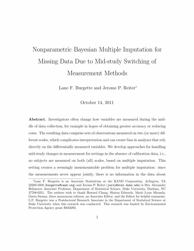
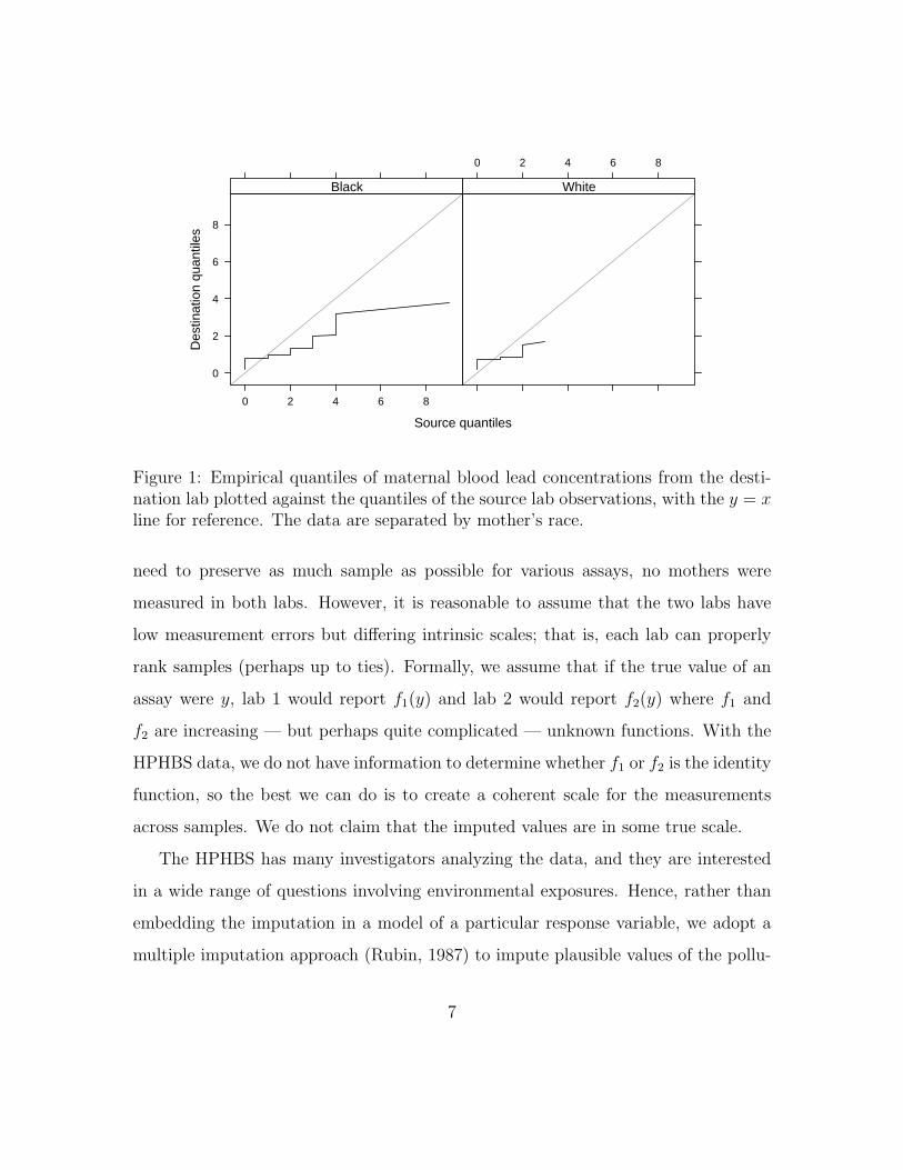
balance of covariates. For example, the quantile-quantile plots in Figure 1 compare

blood lead concentrations reported by the two labs. If the destination lab reported

a smooth version of the source lab’s measurements, we would expect the midpoints

of the nearly horizontal line segments to be close to the y = x line. These plots give

evidence that, for low concentrations, the source lab reports lower values; for higher

true concentrations, the source lab seems to report relatively higher values.

The differences in marginal distributions could result from differences in the back-

ground characteristics of the samples between labs. Indeed, proportionally more

mothers identify their race as white in the lab with finer assay resolution compared

to those who were measured in the original lab. However, within racial groups, other

characteristics of study participants are not appreciably different for the cohorts mea-

sured in the two labs: logistic regressions of lab assignment on a function of tobacco

use, age, and birth weight yield no coefficients that are significant at the 10% level.

Therefore, we attribute within-race differences in the marginal distributions to differ-

ences in the two labs’ measurement methods.

Due to the difficulties of getting blood samples from pregnant women and the

6

Source quantiles

Des

tinat

ion

quan

tiles

0

2

4

6

8

0 2 4 6 8

Black

0 2 4 6 8

White

Figure 1: Empirical quantiles of maternal blood lead concentrations from the desti-nation lab plotted against the quantiles of the source lab observations, with the y = xline for reference. The data are separated by mother’s race.

need to preserve as much sample as possible for various assays, no mothers were

measured in both labs. However, it is reasonable to assume that the two labs have

low measurement errors but differing intrinsic scales; that is, each lab can properly

rank samples (perhaps up to ties). Formally, we assume that if the true value of an

assay were y, lab 1 would report f1(y) and lab 2 would report f2(y) where f1 and

f2 are increasing — but perhaps quite complicated — unknown functions. With the

HPHBS data, we do not have information to determine whether f1 or f2 is the identity

function, so the best we can do is to create a coherent scale for the measurements

across samples. We do not claim that the imputed values are in some true scale.

The HPHBS has many investigators analyzing the data, and they are interested

in a wide range of questions involving environmental exposures. Hence, rather than

embedding the imputation in a model of a particular response variable, we adopt a

multiple imputation approach (Rubin, 1987) to impute plausible values of the pollu-

7

tants on a coherent scale defined by the finer-resolution measurements. In particular,

we use the methods described in Section 4 to create ten completed datasets so that

each mother has either an actual concentration measurement (if she was measured

by the finer-resolution lab) or a set of ten imputed concentration values (if she was

measured by the original, coarser-resolution lab or not measured at all). Investigators

can use complete-data techniques on each imputed dataset, and combine results us-

ing the usual multiple imputation techniques (Rubin, 1987; Reiter and Raghunathan,

2007).

3 DESCRIPTION OF THE METHODS

We now describe the rank permutation (RP), rank-preserving prediction (RPP), and

matched conditional quantile (MCQ) methods. Let Y represent the variable mea-

sured on two different scales, and let X represent the covariates. We suppose that

the values of Y observed in the source scale, yis where i = 1, . . . , ns, are ordered

from smallest to largest, as are the values of Y observed in the destination scale,

yid where i = 1, . . . nd. Let ys and yd be the vectors of all individuals’ observed

data in the source and destination scales, respectively. Let yc denote the complete

set of nc = ns + nd observations in the destination scale. Note that elements of yc

are observed for records in the destination-scale data but missing for records in the

source-scale data.

3.1 Rank Permutation

We begin with RP, which does not explicitly include covariate information in the

imputation process and is simplest to implement computationally. RP relies on the

factorization p(yc|ys,yd) =∫p(yc|rc,ys,yd)p(rc|ys,yd)drc, where rc is the unob-

8

served set of ranks of yc. We assume that p(rc|ys,yd) is a uniform distribution over

all permutations of rc that maintain the marginal ranks of ys and yd; that is, if source

record i has marginal rank r in ys, its rank in rc among only the source records is

also r. This amounts to assuming that the elements of yc are drawn independently

from some common distribution. We sample p(rc|ys,yd) as follows. Consider an urn

with ns red balls for the source observations and nd blue balls for the destination

observations. Sample all nc balls without replacement, numbering each ball after it

is drawn with consecutive numbers from 1 to nc. The numbers on the red balls are a

draw of the ranks of the source-scale measurements if they were transformed into the

destination scale. We sample the missing elements in yc conditional on rc and yd ac-

cording to some distributional estimator applied to yd. For simplicity, we draw from

a discretized version of a Gaussian kernel density estimate (KDE), as implemented

in the density() function in R (Venables and Ripley, 2002; R Development Core

Team, 2010).

For example, suppose that ns = 3 and nd = 2. A drawn sequence from the

urn might be B1R2R3B4R5, with B for blue and R for red. We retain the observed

destination values, so that y1c = y1d and y4c = y2d. We sample values of y2c and y3c

so that y1c < y2c < y3c < y4c. We also sample y5c restricted to be larger than y4c.

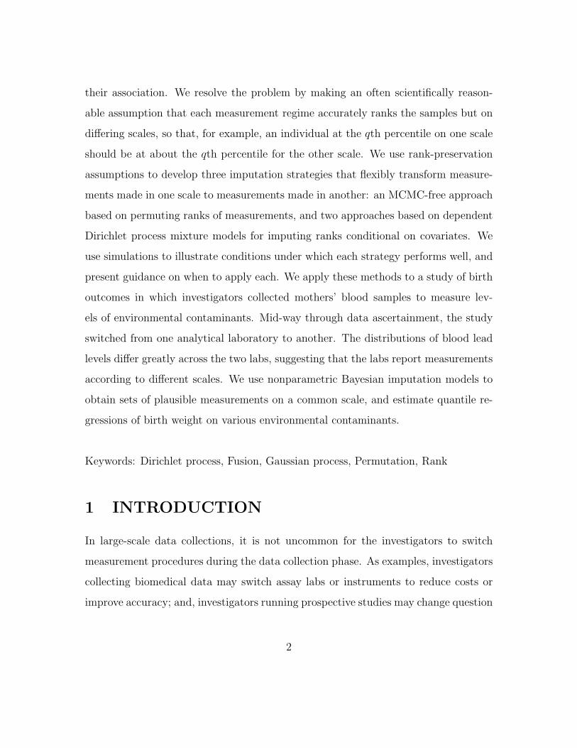
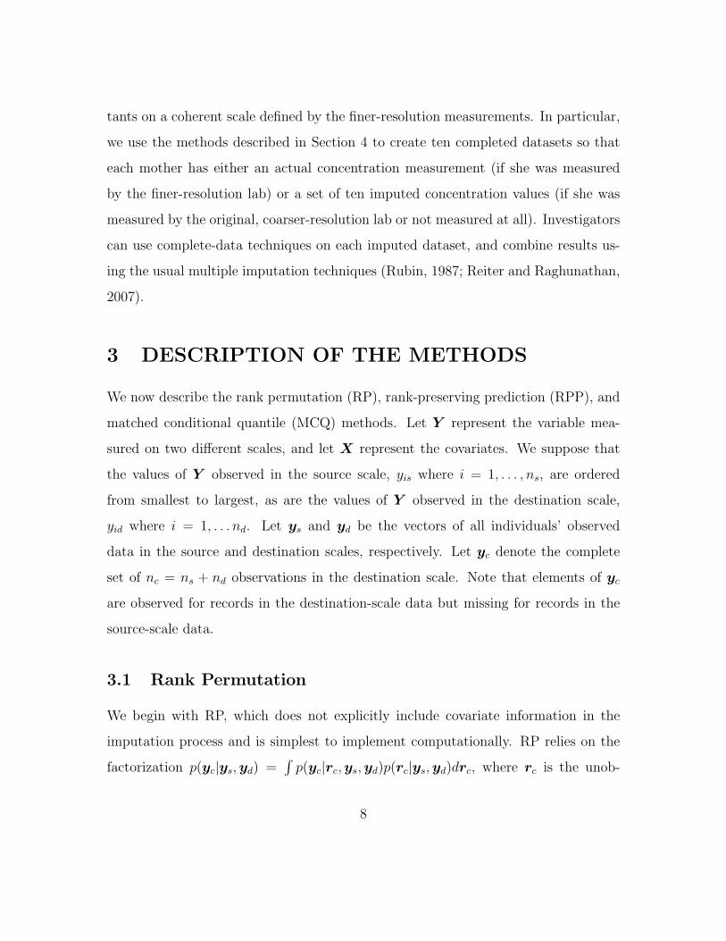
To illustrate the RP method, we consider the following data-generating setup.

The marginal distribution of the nd = 500 destination measurements is standard

normal. We transform from destination to source measurements using f(y) = −2.5 +

5 exp{−.5+.2y}. We then apply RP to impute plausible values of the ns = 200 source

scale measurements in the destination scale. Figure 2 shows the marginal distribution

of yc for ten realizations of RP. The imputed distributions are centered around yd

with uncertainty comparable to the difference between yd and the source observations

after transformation by the true inverse of f . Because RP only uses the ranks of the

9

Den

sity

0.0

0.2

0.4

0.6

−4 −2 0 2 4

Observed scales

−4 −2 0 2 4

Destination scale

Figure 2: Example of the rank permutation (RP) method. The left panel displaysdensity histograms of the observations from the source scale (dashed) and destinationscale (solid). In the right panel, the true density histogram of the transformed valuesis the dashed line. Ten realizations of the RP method are displayed (thin lines), alongwith the observed destination scale measurements (thick gray).

source observations, the right-hand panel would be unchanged if we had used any

other strictly increasing function f .

It is possible to incorporate some auxiliary information by stratifying the observa-

tions according to covariates, and performing RP within each stratum. This approach

can produce imputed values that do not respect the within-scale marginal ranks. It

also can increase variance when sample sizes are small in some strata.

3.2 Rank-Preserving Predictions

RPP is a natural extension of RP, as they both prioritize the preservation of the ob-

served rankings for the source records over other considerations. The key modification

is that RPP overcomes the lack of covariate information in the RP approach, which

10

Covariate

Log

conc

entr

atio

n

−1

0

1

−2 −1 0 1 2

●

● ●●

●

●

Cond. PDF

0.0 0.2 0.4

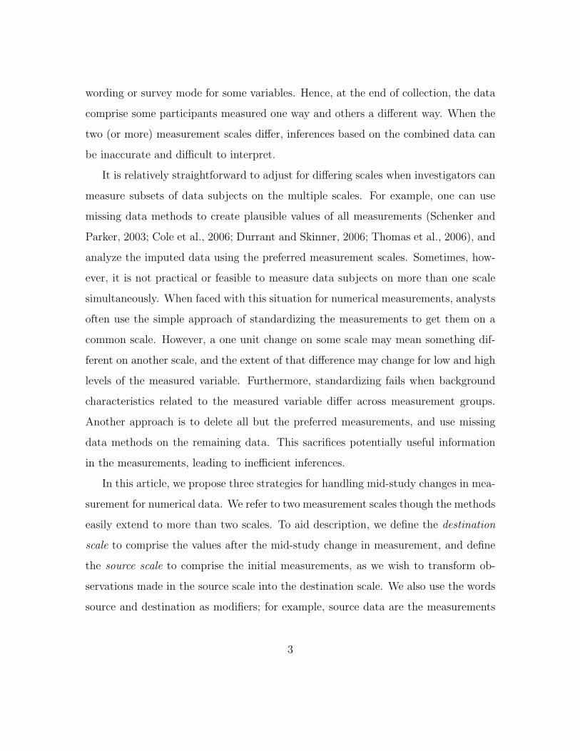
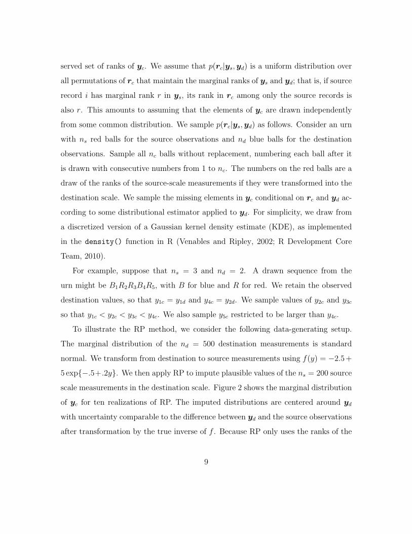
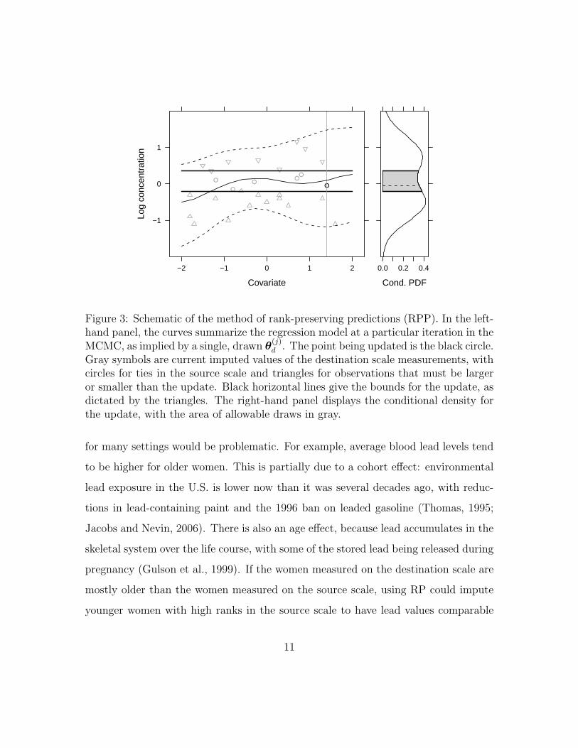
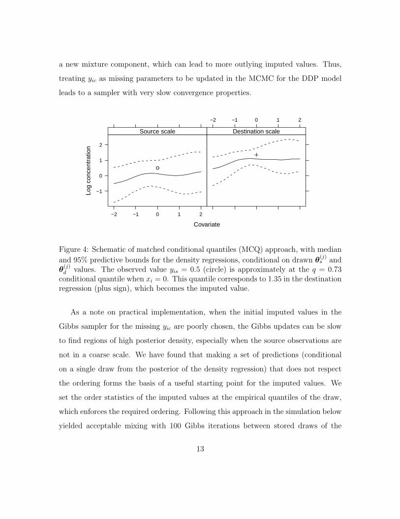
Figure 3: Schematic of the method of rank-preserving predictions (RPP). In the left-hand panel, the curves summarize the regression model at a particular iteration in theMCMC, as implied by a single, drawn θ

(j)d . The point being updated is the black circle.

Gray symbols are current imputed values of the destination scale measurements, withcircles for ties in the source scale and triangles for observations that must be largeror smaller than the update. Black horizontal lines give the bounds for the update, asdictated by the triangles. The right-hand panel displays the conditional density forthe update, with the area of allowable draws in gray.

for many settings would be problematic. For example, average blood lead levels tend

to be higher for older women. This is partially due to a cohort effect: environmental

lead exposure in the U.S. is lower now than it was several decades ago, with reduc-

tions in lead-containing paint and the 1996 ban on leaded gasoline (Thomas, 1995;

Jacobs and Nevin, 2006). There is also an age effect, because lead accumulates in the

skeletal system over the life course, with some of the stored lead being released during

pregnancy (Gulson et al., 1999). If the women measured on the destination scale are

mostly older than the women measured on the source scale, using RP could impute

younger women with high ranks in the source scale to have lead values comparable

11

to those for older women in the destination scale, which would not be appropriate.

To implement RPP, we estimate the conditional distribution of yc given covariates

xc using the destination data. For each source record i, we sample a value of yic

from this conditional distribution with the constraint that the rank of yic among all

source records’ ranks must be preserved; for example, if yis was at the 20th percentile

among source records, then its imputed yic should be at the 20th percentile among

the imputed values for all source records.

More formally, the imputation proceeds in a two step process. First, to estimate

the conditional distribution of yd across the observed covariate space xd, we use

a dependent Dirichlet process (DDP) density regression (MacEachern, 1999); see

Appendices A and B for full description of the model and the MCMC sampling. Let

θd represent the parameters of that model. After MCMC convergence, we sample M

values of θd, where M is the desired number of multiply-imputed datasets. We ensure

that these draws are separated sufficiently in the MCMC iterations so that the θ(j)d ,

where j = 1, . . . ,M , are approximately independent. Second, to impute each source

record’s missing yic, we implement a separate Gibbs sampler for each j as follows.

We set initial starting values for each source record’s yic so that the source ranks are

preserved. We then update yic for each source record sequentially: we sample from

the truncated posterior distribution of yic given θ(j)d with truncation points defined

by the values of yic at the (i − 1)th and (i + 1)th ranks in the source data. This is

shown graphically in Figure 3. This process is repeated until the imputation values

settle down into a stable distribution, and we take one draw from this distribution as

the jth imputed replicate of yc.

One could update the missing yic at each iteration of the MCMC when estimating

the DDP model. However, we have found this can lead to computational difficulties.

In particular, when an outlying yic value is imputed, the model is likely to populate

12

a new mixture component, which can lead to more outlying imputed values. Thus,

treating yic as missing parameters to be updated in the MCMC for the DDP model

leads to a sampler with very slow convergence properties.

Covariate

Log

conc

entr

atio

n

−1

0

1

2

−2 −1 0 1 2

●

Source scale

−2 −1 0 1 2

Destination scale

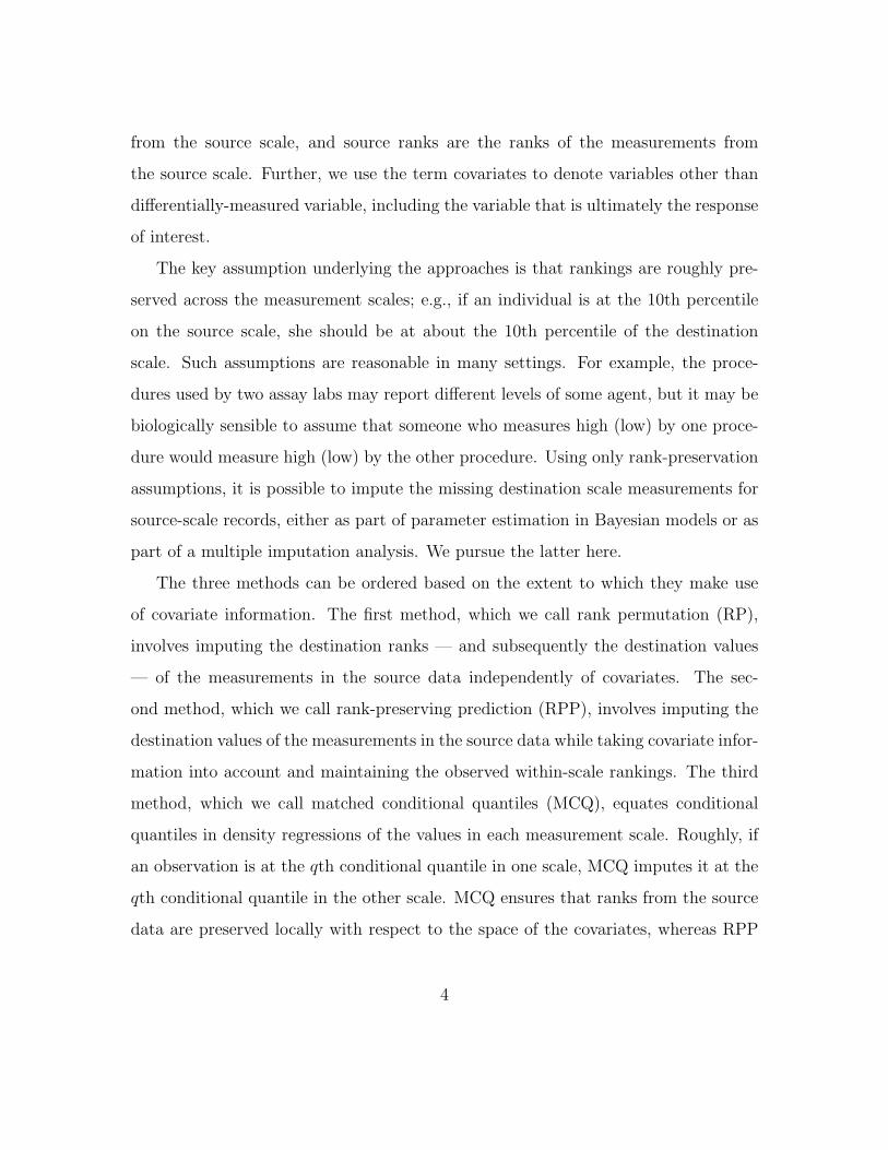
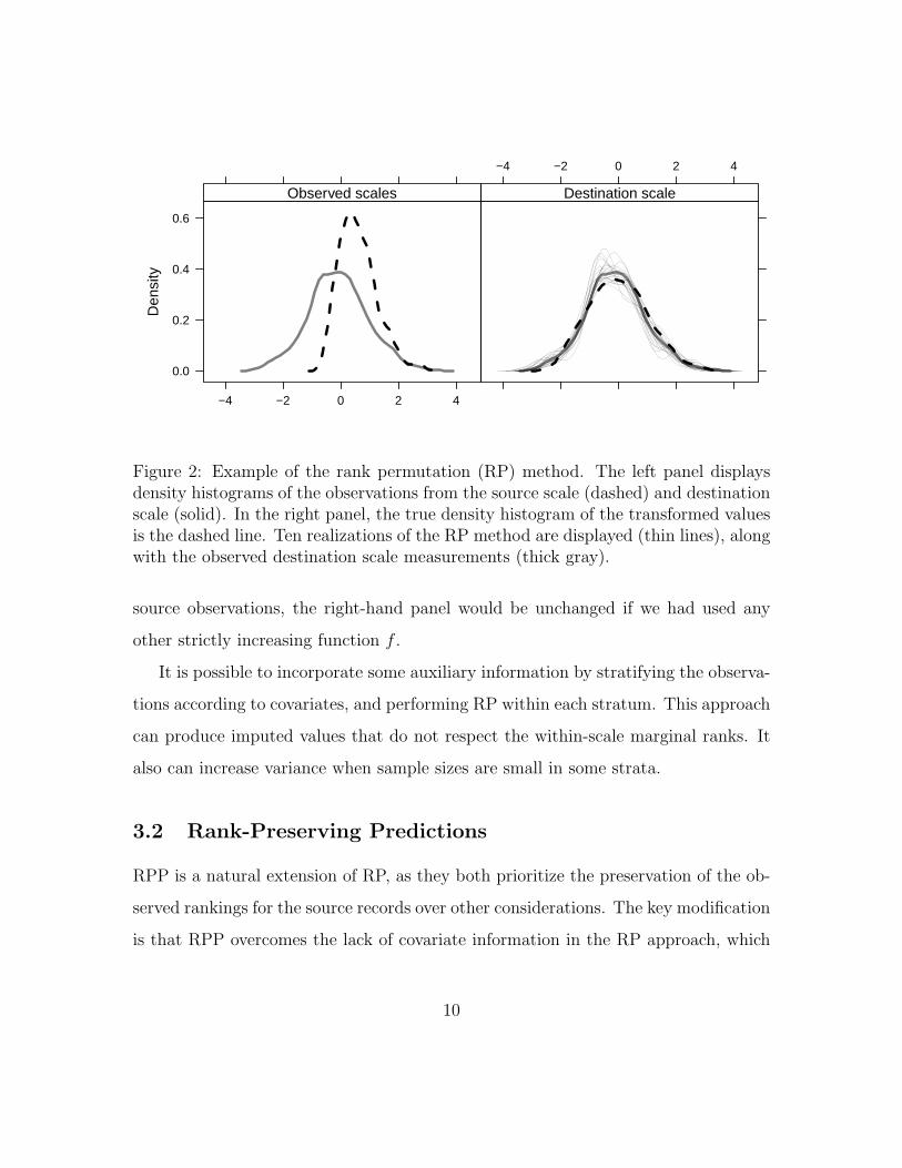
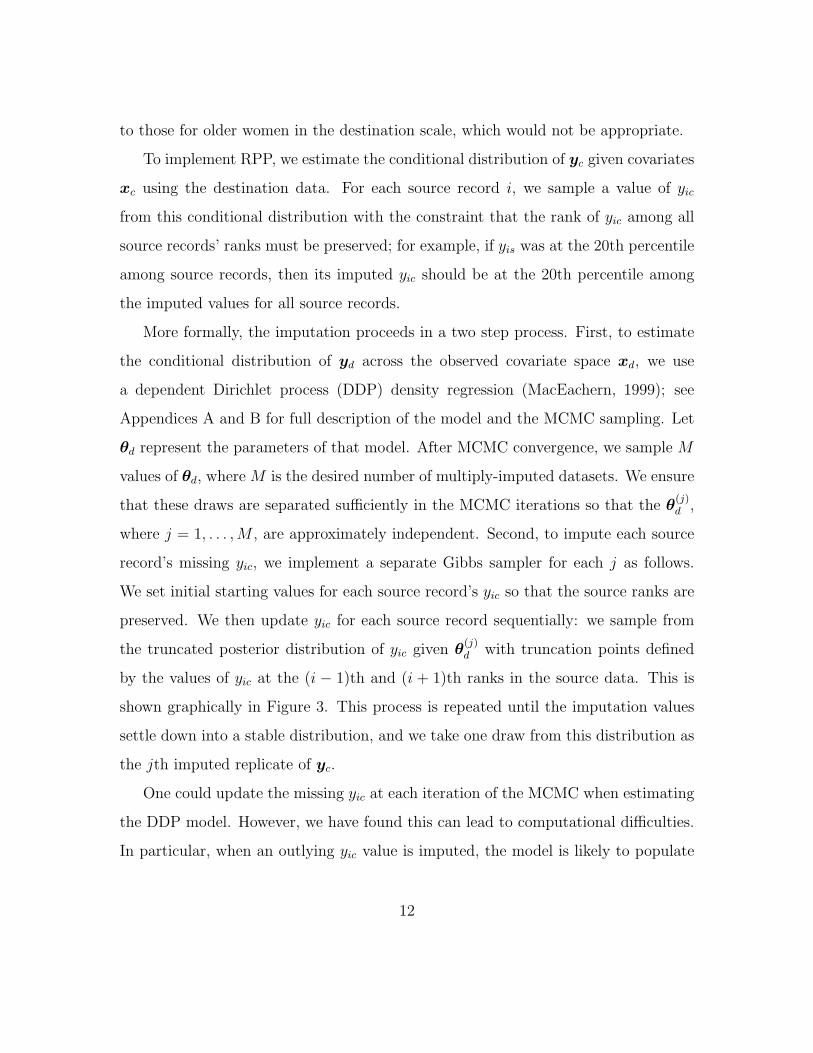
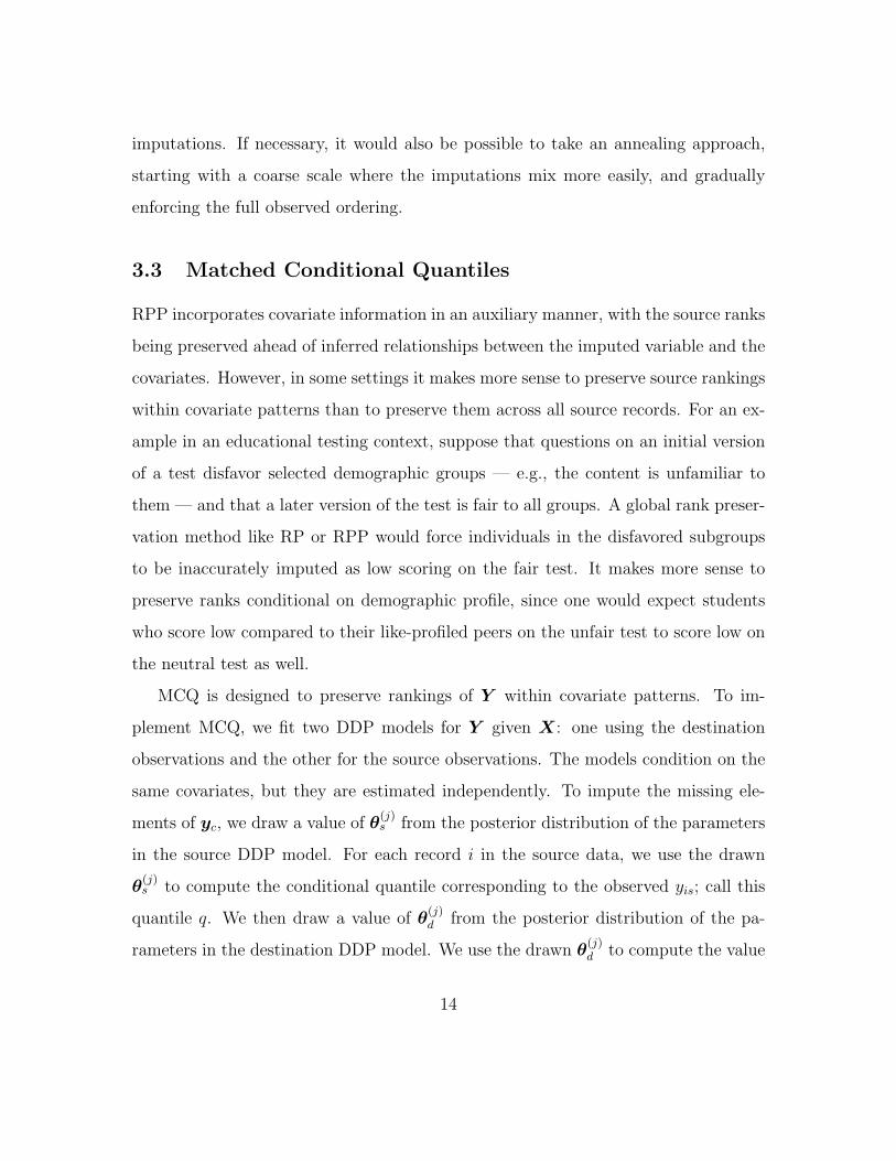
Figure 4: Schematic of matched conditional quantiles (MCQ) approach, with median

and 95% predictive bounds for the density regressions, conditional on drawn θ(j)s and

θ(j)d values. The observed value yis = 0.5 (circle) is approximately at the q = 0.73

conditional quantile when xi = 0. This quantile corresponds to 1.35 in the destinationregression (plus sign), which becomes the imputed value.

As a note on practical implementation, when the initial imputed values in the

Gibbs sampler for the missing yic are poorly chosen, the Gibbs updates can be slow

to find regions of high posterior density, especially when the source observations are

not in a coarse scale. We have found that making a set of predictions (conditional

on a single draw from the posterior of the density regression) that does not respect

the ordering forms the basis of a useful starting point for the imputed values. We

set the order statistics of the imputed values at the empirical quantiles of the draw,

which enforces the required ordering. Following this approach in the simulation below

yielded acceptable mixing with 100 Gibbs iterations between stored draws of the

13

imputations. If necessary, it would also be possible to take an annealing approach,

starting with a coarse scale where the imputations mix more easily, and gradually

enforcing the full observed ordering.

3.3 Matched Conditional Quantiles

RPP incorporates covariate information in an auxiliary manner, with the source ranks

being preserved ahead of inferred relationships between the imputed variable and the

covariates. However, in some settings it makes more sense to preserve source rankings

within covariate patterns than to preserve them across all source records. For an ex-

ample in an educational testing context, suppose that questions on an initial version

of a test disfavor selected demographic groups — e.g., the content is unfamiliar to

them — and that a later version of the test is fair to all groups. A global rank preser-

vation method like RP or RPP would force individuals in the disfavored subgroups

to be inaccurately imputed as low scoring on the fair test. It makes more sense to

preserve ranks conditional on demographic profile, since one would expect students

who score low compared to their like-profiled peers on the unfair test to score low on

the neutral test as well.

MCQ is designed to preserve rankings of Y within covariate patterns. To im-

plement MCQ, we fit two DDP models for Y given X: one using the destination

observations and the other for the source observations. The models condition on the

same covariates, but they are estimated independently. To impute the missing ele-

ments of yc, we draw a value of θ(j)s from the posterior distribution of the parameters

in the source DDP model. For each record i in the source data, we use the drawn

θ(j)s to compute the conditional quantile corresponding to the observed yis; call this

quantile q. We then draw a value of θ(j)d from the posterior distribution of the pa-

rameters in the destination DDP model. We use the drawn θ(j)d to compute the value

14

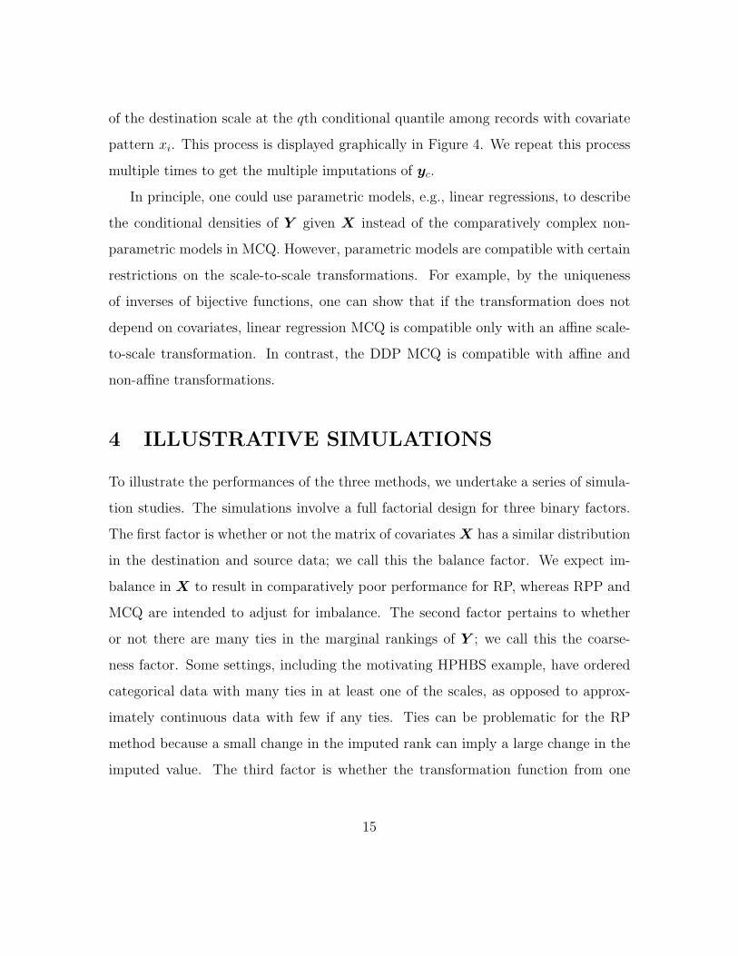
of the destination scale at the qth conditional quantile among records with covariate

pattern xi. This process is displayed graphically in Figure 4. We repeat this process

multiple times to get the multiple imputations of yc.

In principle, one could use parametric models, e.g., linear regressions, to describe

the conditional densities of Y given X instead of the comparatively complex non-

parametric models in MCQ. However, parametric models are compatible with certain

restrictions on the scale-to-scale transformations. For example, by the uniqueness

of inverses of bijective functions, one can show that if the transformation does not

depend on covariates, linear regression MCQ is compatible only with an affine scale-

to-scale transformation. In contrast, the DDP MCQ is compatible with affine and

non-affine transformations.

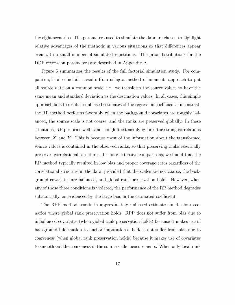
4 ILLUSTRATIVE SIMULATIONS

To illustrate the performances of the three methods, we undertake a series of simula-

tion studies. The simulations involve a full factorial design for three binary factors.

The first factor is whether or not the matrix of covariates X has a similar distribution

in the destination and source data; we call this the balance factor. We expect im-

balance in X to result in comparatively poor performance for RP, whereas RPP and

MCQ are intended to adjust for imbalance. The second factor pertains to whether

or not there are many ties in the marginal rankings of Y ; we call this the coarse-

ness factor. Some settings, including the motivating HPHBS example, have ordered

categorical data with many ties in at least one of the scales, as opposed to approx-

imately continuous data with few if any ties. Ties can be problematic for the RP

method because a small change in the imputed rank can imply a large change in the

imputed value. The third factor is whether the transformation function from one

15

scale to the other preserves ranks of Y globally or only locally. Global preservation

of ranks underlies RPP, whereas local preservation of ranks within covariate patterns

underlies MCQ. In each case, we draw M = 10 copies of yc, and report estimates and

confidence intervals according to the standard multiple imputation combining rules

(Rubin, 1987).

We generate data from this factorial design using one measurement variable Y

and two fully observed variables (X0,X1). We set sample sizes ns = 700 in the source

scale and nd = 300 in the destination scale, which are similar to the sample sizes in

the HPHBS application. For any level of the factorial design, we generate replications

as follows.

• IF BALANCED: Generate Xi,0 ∼ Bern(.5) for all i.

• IF NOT BALANCED: Generate Xi,0 ∼ Bern(pi), where pi = 0.25 for the ns

source observations and pi = 0.75 for the nd destination observations.

• Generate Y = X0 + 0.5N(0, I).

• Generate X1 = X0 + 0.5Y + 0.2N(0, I).

• IF GLOBAL: Transform the source observations via the function f(y) = −.5 exp{−1+

y}.

• IF LOCAL: Transform the source observations via the function f(y;x0) =

−.5 exp{−1 + y − x0}.

• IF COARSE: Round the transformed source observations to the nearest 0.5.

We evaluate the abilities of the methods to estimate the regression coefficient of Y

in the regression of X1 on (Y ,X0). Because of the computational demands of the

MCMC, we limit the simulation study of RPP and MCQ to ten simulations in each of

16

the eight scenarios. The parameters used to simulate the data are chosen to highlight

relative advantages of the methods in various situations so that differences appear

even with a small number of simulated repetitions. The prior distributions for the

DDP regression parameters are described in Appendix A.

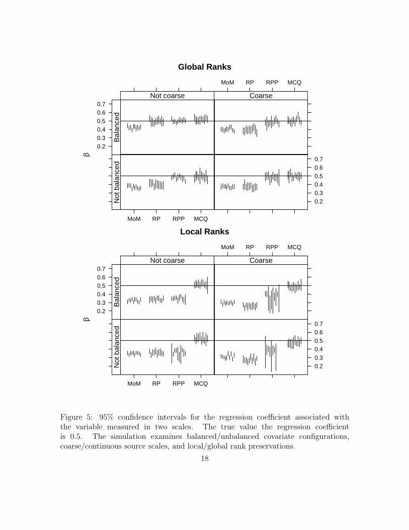
Figure 5 summarizes the results of the full factorial simulation study. For com-

parison, it also includes results from using a method of moments approach to put

all source data on a common scale, i.e., we transform the source values to have the

same mean and standard deviation as the destination values. In all cases, this simple

approach fails to result in unbiased estimates of the regression coefficient. In contrast,

the RP method performs favorably when the background covariates are roughly bal-

anced, the source scale is not coarse, and the ranks are preserved globally. In these

situations, RP performs well even though it ostensibly ignores the strong correlations

between X and Y . This is because most of the information about the transformed

source values is contained in the observed ranks, so that preserving ranks essentially

preserves correlational structures. In more extensive comparisons, we found that the

RP method typically resulted in low bias and proper coverage rates regardless of the

correlational structure in the data, provided that the scales are not coarse, the back-

ground covariates are balanced, and global rank preservation holds. However, when

any of those three conditions is violated, the performance of the RP method degrades

substantially, as evidenced by the large bias in the estimated coefficient.

The RPP method results in approximately unbiased estimates in the four sce-

narios where global rank preservation holds. RPP does not suffer from bias due to

imbalanced covariates (when global rank preservation holds) because it makes use of

background information to anchor imputations. It does not suffer from bias due to

coarseness (when global rank preservation holds) because it makes use of covariates

to smooth out the coarseness in the source scale measurements. When only local rank

17

Global Ranks

β

0.20.30.40.50.60.7

Not coarse

Bal

ance

d

MoM RP RPP MCQ

Coarse

Bal

ance

dMoM RP RPP MCQ

Not coarse

Not

bal

ance

d

0.20.30.40.50.60.7

Coarse

Not

bal

ance

d

Local Ranks

β

0.20.30.40.50.60.7

Not coarse

Bal

ance

d

MoM RP RPP MCQ

Coarse

Bal

ance

d

MoM RP RPP MCQ

Not coarse

Not

bal

ance

d

0.20.30.40.50.60.7

Coarse

Not

bal

ance

d

Figure 5: 95% confidence intervals for the regression coefficient associated withthe variable measured in two scales. The true value the regression coefficientis 0.5. The simulation examines balanced/unbalanced covariate configurations,coarse/continuous source scales, and local/global rank preservations.

18

preservation holds, RPP results not only in biased estimates, but some of the intervals

have large widths. This results from the poor fit of models that incorrectly presume

globally rank-preserved predictions, which can yield widely-spaced modes for the im-

puted quantities. This in turn can result in parameter estimates that vary greatly

from imputation to imputation, which translates into wide confidence intervals.

The MCQ method is the only method that results in approximately unbiased

estimates in all eight scenarios. However, this flexibility comes with a price: the

intervals can have comparatively larger widths. For example, in the balanced and

not coarse condition with globally-preserved ranks, the confidence intervals resulting

from RPP are uniformly narrower than those from MCQ, while still displaying good

coverage. Also, if it is the case that the source scale has few observations, we would

expect the source scale model to be quite sensitive to the prior specification.

Across all scenarios, any biases attenuate the true effect. This consistent attenua-

tion is intentional: we arranged the simulation so that biases of opposite signs would

not cancel. In general, it is possible for the biases to be positive or negative.

Preserveglobal ranks?

Use MCQ

No

Coarse measure-ments and/or

imbalanced X?

Use RP

No

Use RPP

Yes

Yes

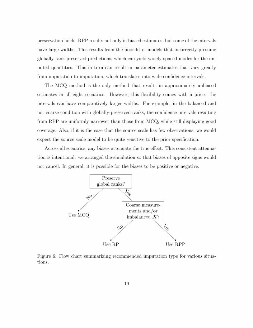
Figure 6: Flow chart summarizing recommended imputation type for various situa-tions.

19

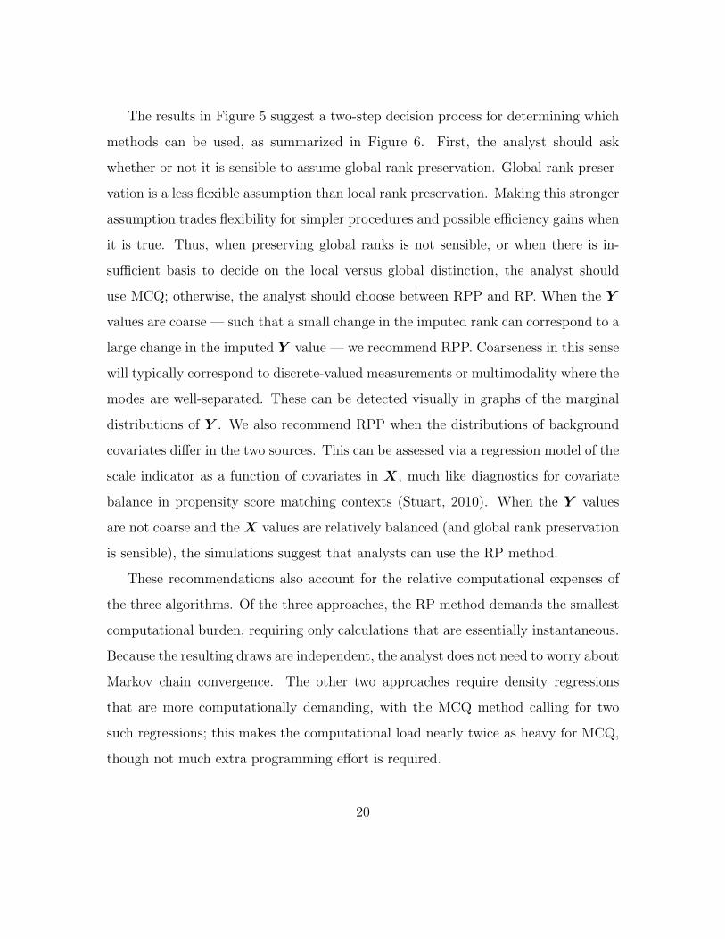
The results in Figure 5 suggest a two-step decision process for determining which

methods can be used, as summarized in Figure 6. First, the analyst should ask

whether or not it is sensible to assume global rank preservation. Global rank preser-

vation is a less flexible assumption than local rank preservation. Making this stronger

assumption trades flexibility for simpler procedures and possible efficiency gains when

it is true. Thus, when preserving global ranks is not sensible, or when there is in-

sufficient basis to decide on the local versus global distinction, the analyst should

use MCQ; otherwise, the analyst should choose between RPP and RP. When the Y

values are coarse — such that a small change in the imputed rank can correspond to a

large change in the imputed Y value — we recommend RPP. Coarseness in this sense

will typically correspond to discrete-valued measurements or multimodality where the

modes are well-separated. These can be detected visually in graphs of the marginal

distributions of Y . We also recommend RPP when the distributions of background

covariates differ in the two sources. This can be assessed via a regression model of the

scale indicator as a function of covariates in X, much like diagnostics for covariate

balance in propensity score matching contexts (Stuart, 2010). When the Y values

are not coarse and the X values are relatively balanced (and global rank preservation

is sensible), the simulations suggest that analysts can use the RP method.

These recommendations also account for the relative computational expenses of

the three algorithms. Of the three approaches, the RP method demands the smallest

computational burden, requiring only calculations that are essentially instantaneous.

Because the resulting draws are independent, the analyst does not need to worry about

Markov chain convergence. The other two approaches require density regressions

that are more computationally demanding, with the MCQ method calling for two

such regressions; this makes the computational load nearly twice as heavy for MCQ,

though not much extra programming effort is required.

20

5 APPLICATION TO ASSAY LAB CHANGES

We now turn to the mid-study lab assay change in the HPHBS. We focus on mea-

surements of blood lead levels, although some of the other metals also had dissimilar

distributions in the two labs. Of the 1435 women, 323 have blood lead levels measured

on the destination scale; 807 are measured on the source scale; and, the remainder

are missing a lead measurement. Although typically one would rather the destination

scale have more observations than the source scale so as to reduce reliance on impu-

tations, the investigators specified the second set of measurements as the destination

scale because it offers finer resolution and lower detection limits. We also transform

to the log concentration scale so that negative imputations are not a concern.

Based on scientific grounds, we find little reason to believe that one or both of the

labs would use a scale that reports different measurements depending on background

covariates. Hence, we believe it is sensible to assume global rank preservation when

imputing to a common scale. Therefore, we do not use MCQ. As mentioned in

Section 2, maternal race is not balanced across laboratory assignments. Additionally,

the source lab observations are coarse, as they are reported in an integer-valued scale

(Figure 1). For these reasons, we prefer RPP over RP. As covariates in X, we include

race, age, self-reported smoking status (non-smoker, quit, smoker), and birth weight

rounded to the nearest 500g. Exploratory regression analyses indicate that these

variables are associated with lead levels. See Appendix A for discussions of the prior

distributions used in the RPP.

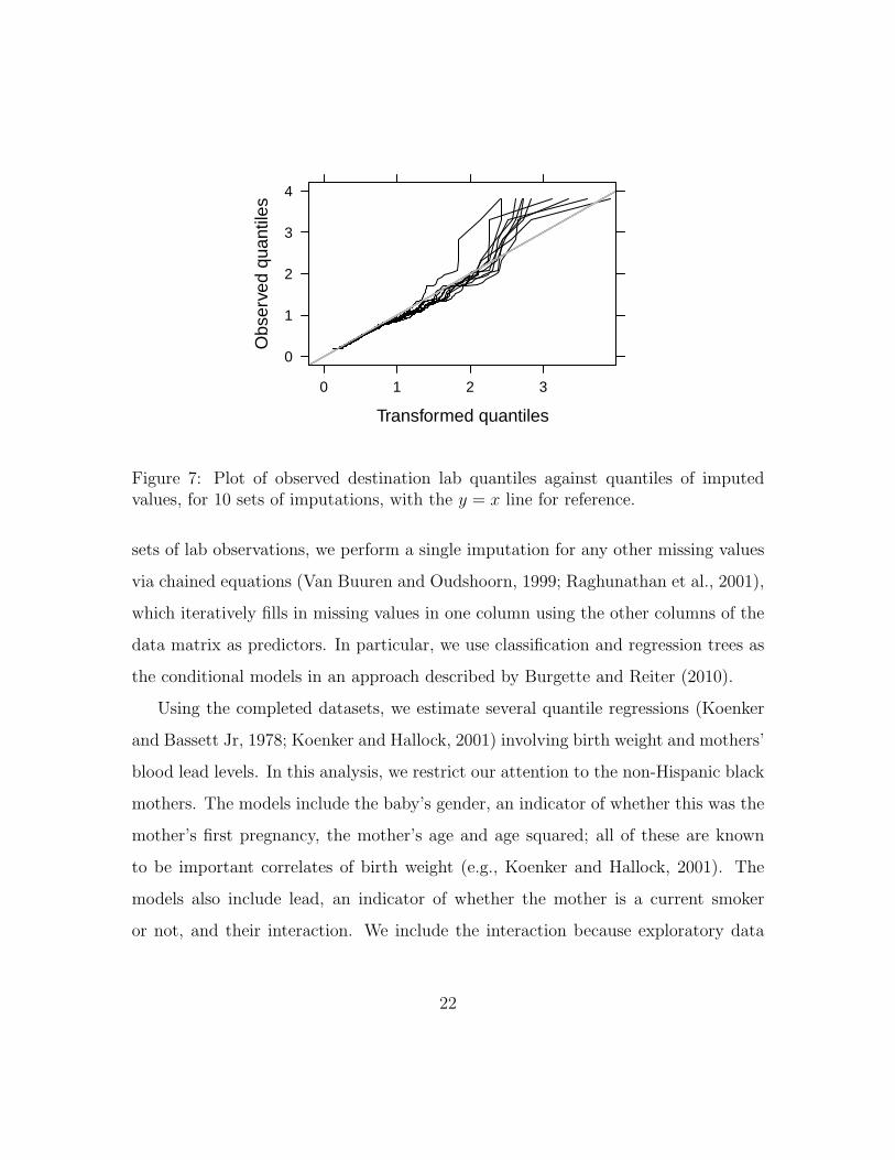
The data have missing values for several other variables, although the covariates

in the models for RPP are essentially fully observed. We first run the RPP method

to form M = 10 completed sets of lead observations in the destination lab scale. As

shown in Figure 7, the distributions of the transformed source lab measurements are

comparable to the observed destination lab measurements. For each of the completed

21

0

1

2

3

4

0 1 2 3

0

1

2

3

4

0 1 2 3

0

1

2

3

4

0 1 2 3

0

1

2

3

4

0 1 2 3

0

1

2

3

4

0 1 2 3

0

1

2

3

4

0 1 2 3

0

1

2

3

4

0 1 2 3

0

1

2

3

4

0 1 2 3

0

1

2

3

4

0 1 2 3

Transformed quantiles

Obs

erve

d qu

antil

es

0

1

2

3

4

0 1 2 3

Figure 7: Plot of observed destination lab quantiles against quantiles of imputedvalues, for 10 sets of imputations, with the y = x line for reference.

sets of lab observations, we perform a single imputation for any other missing values

via chained equations (Van Buuren and Oudshoorn, 1999; Raghunathan et al., 2001),

which iteratively fills in missing values in one column using the other columns of the

data matrix as predictors. In particular, we use classification and regression trees as

the conditional models in an approach described by Burgette and Reiter (2010).

Using the completed datasets, we estimate several quantile regressions (Koenker

and Bassett Jr, 1978; Koenker and Hallock, 2001) involving birth weight and mothers’

blood lead levels. In this analysis, we restrict our attention to the non-Hispanic black

mothers. The models include the baby’s gender, an indicator of whether this was the

mother’s first pregnancy, the mother’s age and age squared; all of these are known

to be important correlates of birth weight (e.g., Koenker and Hallock, 2001). The

models also include lead, an indicator of whether the mother is a current smoker

or not, and their interaction. We include the interaction because exploratory data

22

analyses of Burgette et al. (2011) suggested it may be important. We note that these

exploratory analyses were performed using only the source lab lead measurements.

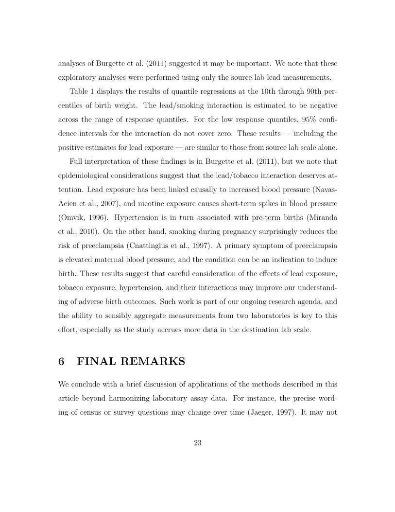
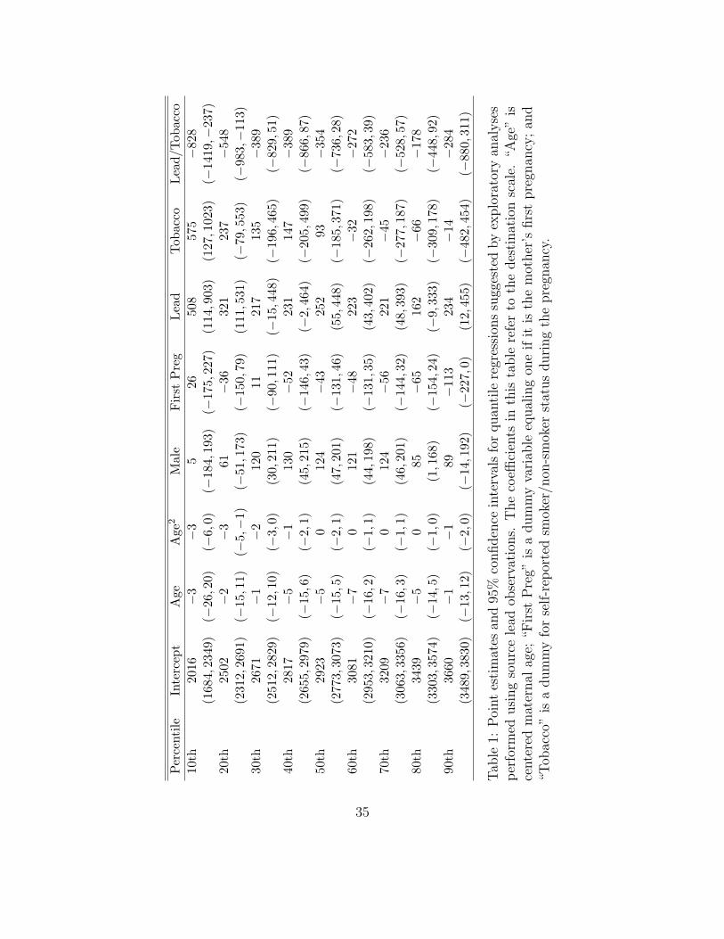
Table 1 displays the results of quantile regressions at the 10th through 90th per-

centiles of birth weight. The lead/smoking interaction is estimated to be negative

across the range of response quantiles. For the low response quantiles, 95% confi-

dence intervals for the interaction do not cover zero. These results — including the

positive estimates for lead exposure — are similar to those from source lab scale alone.

Full interpretation of these findings is in Burgette et al. (2011), but we note that

epidemiological considerations suggest that the lead/tobacco interaction deserves at-

tention. Lead exposure has been linked causally to increased blood pressure (Navas-

Acien et al., 2007), and nicotine exposure causes short-term spikes in blood pressure

(Omvik, 1996). Hypertension is in turn associated with pre-term births (Miranda

et al., 2010). On the other hand, smoking during pregnancy surprisingly reduces the

risk of preeclampsia (Cnattingius et al., 1997). A primary symptom of preeclampsia

is elevated maternal blood pressure, and the condition can be an indication to induce

birth. These results suggest that careful consideration of the effects of lead exposure,

tobacco exposure, hypertension, and their interactions may improve our understand-

ing of adverse birth outcomes. Such work is part of our ongoing research agenda, and

the ability to sensibly aggregate measurements from two laboratories is key to this

effort, especially as the study accrues more data in the destination lab scale.

6 FINAL REMARKS

We conclude with a brief discussion of applications of the methods described in this

article beyond harmonizing laboratory assay data. For instance, the precise word-

ing of census or survey questions may change over time (Jaeger, 1997). It may not

23

be practical to ask individuals multiple versions of the same question, yet longitu-

dinal comparisons may require data on common scales. In large-scale epidemiologic

or psycho-social contexts, analysts may seek to combine information from multiple

datasets in which key variables are measured or defined differently. Without access

to a validation sample on which individuals are measured with the multiple methods,

these methods can offer an approach to data harmonization. In education and other

contexts, there can be significant rater-to-rater differences (Johnson, 1996). If these

differences are not simply additive shifts, it may be desirable to flexibly put all raters’

scores on one scale.

APPENDIX A: MODELS FOR RPP AND MCQ

The RPP and MCQ methods use dependent Dirichlet process (DDP) regressions

to estimate conditional distributions of the measurements given covariates. In this

appendix, we review DDP models and describe their implementation for RPP and

MCQ.

Recent Bayesian research has demonstrated the flexibility of mixture modeling

approaches (e.g., Escobar and West, 1995; Muller et al., 1996; Griffin and Steel,

2006; Dunson et al., 2007; Dunson and Park, 2008). The Dirichlet process (DP)

(Ferguson, 1973; Blackwell and MacQueen, 1973) has become a popular choice for

the mixing distribution in such models. Technically, the DP describes a distribution

on a collection of distributions that are defined on some measurable space Θ. The DP

is parametrized by a base measure G0 defined on Θ and a concentration parameter

α, which we will write G ∼ DP(α,G0).

Sethuraman (1994) showed that the DP can be constructed via a stick-breaking

process. If G ∼ DP(α,G0), then we can write G =∑∞

j=1 pjδθj where θjiid∼G0 and

24

p = {pj} are specified as pj = vj∏j−1

k=1(1 − vk) where vkiid∼ beta(1, α). This is often

written as p ∼ GEM(α).

The dependent Dirichlet process (DDP) (MacEachern, 1999; De Iorio et al., 2004;

Gelfand et al., 2005) induces a DP at each covariate value, but allows for flexible

sharing of information across the covariate space. We adopt the DDP that takes on

the form

G(x) =∞∑j=1

pjδηj(x), with ηjiid∼G0X (1)

where ηj are IID realizations of a base Gaussian process (GP) G0X defined on the

covariate space X (Fronczyk and Kottas, 2010). This is a “single p” DDP, as the pj

values are fixed across the covariate space.

Sharing of information across covariate values is a consequence of the continuity of

realizations of the base stochastic process G0X (e.g., Rasmussen and Williams, 2006).

Given hyperparameters, G0X is parametrized so that E(ηj(xi)) = x′iβ, Var(ηj(xi)) =

σ2η, Corr(ηj(xi), ηj(xj)|φ) = exp(−φ|xi − xj|2) with φ > 0 for any xi,xj ∈ X (Fron-

czyk and Kottas, 2010). We collect these parameters as ψ = (β, σ2η, φ).

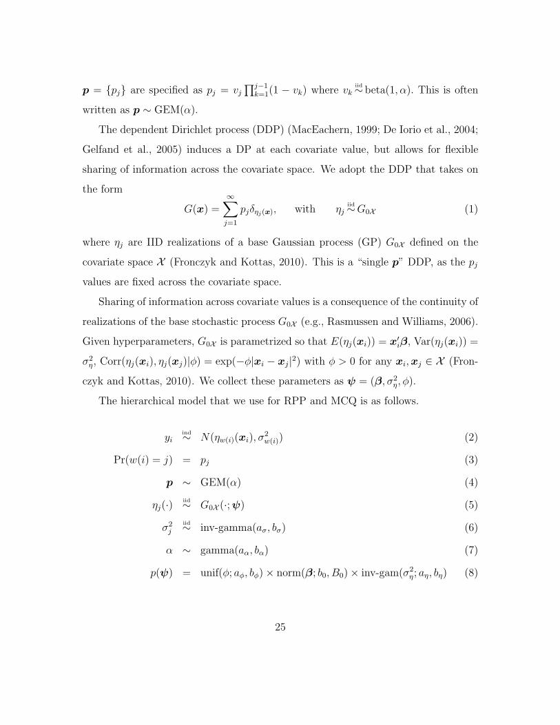
The hierarchical model that we use for RPP and MCQ is as follows.

yiind∼ N(ηw(i)(xi), σ

2w(i)) (2)

Pr(w(i) = j) = pj (3)

p ∼ GEM(α) (4)

ηj(·)iid∼ G0X (·;ψ) (5)

σ2j

iid∼ inv-gamma(aσ, bσ) (6)

α ∼ gamma(aα, bα) (7)

p(ψ) = unif(φ; aφ, bφ)× norm(β; b0, B0)× inv-gam(σ2η; aη, bη) (8)

25

For RPP, we use only the measurements from the source scale to fit the model.

For MCQ, we fit the model separately for the source scale and the destination scale

measurements. We standardize all covariates to have mean zero and variance one

before estimating the models.

To specify the hyperparameters, we monitored the predicted conditional quan-

tiles of the density regressions, searching for values that gave predicted quantiles that

were compatible with those observed in the observed Y . We found reasonable pre-

dicted quantiles when setting aα = bα = 1 and aη = 1/bη = 5; assuming that φ

is uniform on [.5, 15]; and assuming that the β components follow standard normal

prior distributions. In both our simulated examples and the HPHBS, checks of the

posterior predicted quantiles indicated little sensitivity to making these prior distri-

butions more or less diffuse. We therefore used these specifications. We recommend

that analysts start with these values as defaults, and titrate as necessary if posterior

predicted quantiles do not accord with observed values.

In the HPHBS, the posterior densities were sensitive to the prior distribution for

σ2j . When the expected variance was too big, upper and lower quantiles of Y tended

to be well outside the observed range of values. When the expected variance was

too small, we found the posterior predictive distributions were too tight. With this

in mind, for the HPHBS we set aσ = 10 and bσ = 1, which corresponds to a prior

95% interval for the conditional standard deviation of approximately (.24, .46). The

range of the observed log destination lab observations is approximately 3.0, so the

mixing over GPs with standard deviations implied by that prior seems reasonable.

We recommend that analysts tune priors in a similar process, using comparisons of

quantiles of the posterior predictive distribution to the observed values to check the

suitability of the prior specification.

For the illustrative simulations, we typically set aσ = 2.5 and bσ = 1. In the

26

case of the unbalanced/biased/coarse experimental setup, this resulted in overly wide

posterior predictive intervals, so we set aσ = 3.5.

We truncated the DP so that the stick-breaking representation is G =∑L

j=1 pjδθj

by assigning pL = 1−∑L−1

k=1 pk for a fixed L. We truncated at L = 15, as monitoring

the p values indicates that little posterior mass would be allocated to later mixture

components in our applications. Use of a finite L allows us to use the blocked Gibbs

sampler of Ishwaran and James (2002), which samples the mixture components w(i)

jointly; see also Ishwaran and James (2001). It is also possible to use the full DP and

sample the mixture components via a Polya urn representation conditioning on the

other the others.

When observations yi are rounded to a small number of possible outcome val-

ues, or when there is a known detection limit associated with the measurement, the

conditional normality implied by our model may be unrealistic. In such cases we

augment the model with latent quantities that represent the pre-rounding quantity,

or the quantity that was not truncated at the detection limit. This standard data

augmentation method is straightforward to add to the proposed model (Tanner and

Wong, 1987).

The squared exponential covariance function in the model results in a very smooth

stochastic process. This covariance also implies rapid degradation of the correlations.

Rasmussen and Williams (2006) describe alternative correlation structures useful if

either of these properties is undesirable for a particular application. When the data

are such that the GP covariance matrix is close to singular with reasonable values of

ψ, it is common to add a “jitter” matrix of the form cI to the covariance for a small

c > 0 in order to ensure numerical stability. See Savitsky et al. (2011) for discussion

of this and other approaches for stabilizing GP computations, and considerations for

choosing the covariance structure.

27

APPENDIX B: MCMC DETAILS

Following Rasmussen and Williams (2006), we use K(X1,X2) to denote matrix of

pairwise GP covariances (conditional on the mixture indictor) between the points

described by the rows of X1 and X2. We factor K(X1,X2) = σ2ηH(φ). Further, we

denote with Xu the matrix of unique predictor values.

Updates should be as follows:

1. Update ηj evaluated at Xu for j = 1, . . . , L.

• If no observations are currently assigned to the jth mixture component,

then ηj(Xu) ∼ N(Xuβ,K(Xu,Xu)).

• Else, ηj(Xu)|all ∼ normal(µη,Ση) where

µη = Xuβ +K(Xu,Xj)[K(Xj,Xj) + σ2jI]−1(yj −Xjβ)

Ση = K(Xu,Xu)−K(Xu,Xj)[K(Xl,Xl) + σ2jI]−1K(Xj,Xu).

Here, Xj and yj collect the observations that are assigned to the jth

mixture component. (See Chapter 2 of Rasmussen and Williams (2006).)

2. For j = 1, . . . , L, update

σ2j ∼ inv-gamma(aσ + .5n∗j , bσ + .5

∑i:w(i)=j

(yi − ηj(xi))2)

where n∗j counts the number of elements assigned to the jth mixture component.

3. For i = 1, . . . , n, sample w(i) ∼∑L

j=1 pjδj(w(i)) where pj ∝ pjN(yi; ηj(xi), σ2j ).

4. Update p ∼ generalized-Dir((n∗1, . . . , n∗L−1+1); (α+

∑Lj=2 n

∗k, . . . , α+n∗L)), which

can be sampled as described in Ishwaran and James (2002) or Fronczyk and

28

Kottas (2010).

5. Sample α ∼ gamma(shape = L+ aα, rate = bα − log(pL)).

6. Sample β ∼ normal(β,B−1) where B = n∗ηX′uK

−1Xu +B0 and

β = B−1∑

j:n∗j>0XuK−1ηj(Xu). Here, K is shorthand for K(Xu,Xu), and

n∗η counts the number of mixture components that have at least one assigned

observation.

7. Following Fronczyk and Kottas (2010), we specify the prior p(φ) ∝ 1{φ < bφ}.

We also require φ > aφ for a small aφ to avoid proposingH(φ) matrices that are

ill-conditioned. We sample φ in a random walk MH step with the conditional

density proportional to

|H(φ)|−n∗η/2 exp

(−.5σ−2

η

∑j:n∗j>0

(ηj(Xu)−Xuβ)′H−1(φ)(ηj(Xu)−Xuβ)

)1{aφ < φ < bφ}.

8. Sample

σ2η ∼ inv-gamma(aη+.5n

∗η, bη+.5

∑j:n∗j>0

(ηj(Xu)−Xuβ)′H−1(φ)(ηj(Xu)−Xuβ)).

To generate M completed datasets, record M approximately independent draws

of the parameters from the density regression described above. For each of these M

draws, sample imputed values in the destination scale as follows:

For RPP, generate a starting set of imputed values. Then repeatedly update the

imputed values one at a time. Let bL be the maximum of the current imputed values

that are required to be smaller than the observation whose value we are updating. Let

bU be the minimum of the observations that are required to be larger. We then wish to

update the imputed value from the conditional density, restricted to be in the interval

29

(bL, bU). To achieve this, first calculate the probability that the restricted draw will

come from the jth mixture component, which is proportional to pj[Φ(bU ; ηj(xi), σ2j )−

Φ(bL; ηj(xi), σ2j )], where Φ is the normal CDF. After sampling the mixture indicator,

sample the imputed value according to a truncated univariate normal distribution.

Observations without a measurement in either scale are easily handled: simply impute

into the destination scale without any truncation in the conditional distributions.

For MCQ, determine the conditional quantile for each source observation in the

source scale, which is described by a linear combination of normal CDF values. Nu-

merically invert the conditional CDFs in the destination scale to produce the imputed

values.

References

Blackwell, D., and MacQueen, J. (1973), “Ferguson distributions via Polya urn

schemes,” The Annals of Statistics, 1(2), 353–355.

Burgette, L. F., and Reiter, J. P. (2010), “Multiple imputation for missing data via

sequential regression trees,” American Journal of Epidemiology, 172(9), 1070–1076.

Burgette, L., Reiter, J., and Miranda, M. (2011), “Exploratory quantile regression

with many covariates: An application to adverse birth outcomes,” Epidemiology,

22(6), 2721–2735.

Cnattingius, S., Mills, J., Yuen, J., Eriksson, O., and Salonen, H. (1997), “The

paradoxical effect of smoking in preeclamptic pregnancies: Smoking reduces the

incidence but increases the rates of perinatal mortality, abruptio placentae, and

intrauterine growth restriction,” American Journal of Obstetrics and Gynecology,

177(1), 156–161.

30

Cole, S. R., Chu, H., and Greenland, S. (2006), “Multiple-imputation for

measurement-error correction,” International Journal of Epidemiology, 35, 1074–

1081.

De Iorio, M., Mueller, P., Rosner, G., and MacEachern, S. (2004), “An ANOVA model

for dependent random measures,” Journal of the American Statistical Association,

99(465), 205–215.

Dunson, D., and Park, J. (2008), “Kernel stick-breaking processes,” Biometrika,

95(2), 307.

Dunson, D., Pillai, N., and Park, J. (2007), “Bayesian density regression,” Journal of

the Royal Statistical Society: Series B, 69(2), 163–183.

Durrant, G. B., and Skinner, C. (2006), “Using missing data methods to correct for

measurement error in a distribution function,” Survey Methodology, 32, 25–36.

Escobar, M., and West, M. (1995), “Bayesian density estimation and inference using

mixtures,” Journal of the American Statistical Association, 90(430).

Ferguson, T. (1973), “A Bayesian analysis of some nonparametric problems,” The

Annals of Statistics, 1(2), 209–230.

Fronczyk, K., and Kottas, A. (2010), “A Bayesian nonparametric modeling framework

for developmental toxicity studies,” University of California, Santa Cruz Technical

Report, UCSC-SOE-10(11), 1–34.

Gelfand, A., Kottas, A., and MacEachern, S. (2005), “Bayesian nonparametric spa-

tial modeling with Dirichlet process mixing,” Journal of the American Statistical

Association, 100(471), 1021–1035.

31

Griffin, J., and Steel, M. (2006), “Order-based dependent Dirichlet processes,” Jour-

nal of the American Statistical Association, 101(473), 179–194.

Gulson, B., Pounds, J., Mushak, P., Thomas, B., Gray, B., and Korsch, M. (1999),

“Estimation of cumulative lead releases (lead flux) from the maternal skeleton

during pregnancy and lactation,” The Journal of Laboratory and Clinical Medicine,

134(6), 631–640.

Ishwaran, H., and James, L. (2001), “Gibbs sampling methods for stick-breaking

priors,” Journal of the American Statistical Association, 96(453), 161–173.

Ishwaran, H., and James, L. (2002), “Approximate Dirichlet process computing

in finite normal mixtures,” Journal of Computational and Graphical Statistics,

11(3), 508–532.

Jacobs, D., and Nevin, R. (2006), “Validation of a 20-year forecast of US childhood

lead poisoning: Updated prospects for 2010,” Environmental Research, 102(3), 352–

364.

Jaeger, D. (1997), “Reconciling the old and new census bureau education questions:

Recommendations for researchers,” Journal of Business and Economic Statistics,

15(3), 300–309.

Johnson, V. (1996), “On Bayesian analysis of multirater ordinal data: An application

to automated essay grading.,” Journal of the American Statistical Association,

91(433), 42–51.

Koenker, R., and Bassett Jr, G. (1978), “Regression quantiles,” Econometrica,

46(1), 33–50.

32

Koenker, R., and Hallock, K. (2001), “Quantile regression,” Journal of Economic

Perspectives, 15(4), 143–156.

MacEachern, S. (1999), Dependent nonparametric processes,, in Proceedings of the

Section on Bayesian Statistical Science, pp. 50–55.

Miranda, M., Swamy, G., Edwards, S., Maxson, P., Gelfand, A., and James, S.

(2010), “Disparities in maternal hypertension and pregnancy outcomes: Evidence

from North Carolina, 1994–2003,” Public Health Reports, 125(4), 579.

Muller, P., Erkanli, A., and West, M. (1996), “Bayesian curve fitting using multivari-

ate normal mixtures,” Biometrika, 83(1), 67.

Navas-Acien, A., Guallar, E., Silbergeld, E., and Rothenberg, S. (2007), “Lead ex-

posure and cardiovascular disease—A systematic review,” Environmental Health

Perspectives, 115(3), 472.

Omvik, P. (1996), “How smoking affects blood pressure,” Blood Pressure, 5(2), 71.

R Development Core Team (2010), R: A Language and Environment for Statistical

Computing, R Foundation for Statistical Computing, Vienna, Austria. ISBN 3-

900051-07-0.

Raghunathan, T., Lepkowski, J., Van Hoewyk, J., and Solenberger, P. (2001), “A

multivariate technique for multiply imputing missing values using a sequence of

regression models,” Survey methodology, 27(1), 85–96.

Rasmussen, C., and Williams, C. (2006), Gaussian Processes for Machine Learning,

Cambridge, MA: MIT Press.

Reiter, J. P., and Raghunathan, T. E. (2007), “The multiple adaptations of multiple

imputation,” Journal of the American Statistical Association, 102, 1462–1471.

33

Rubin, D. (1987), Multiple Imputation for Nonresponse in Surveys, New York, NY:

John Wiley.

Savitsky, T., Vannucci, M., and Sha, N. (2011), “Variable selection for nonparametric

Gaussian process priors: Models and computational strategies,” Statistical Science,

26(1), 130–149.

Schenker, N., and Parker, J. D. (2003), “From single-race reporting to multiple-

race reporting: Using imputation methods to bridge the transition,” Statistics in

Medicine, 22, 1571–1587.

Sethuraman, J. (1994), “A constructive definition of Dirichlet priors,” Statistica

Sinica, 4(2), 639–650.

Stuart, E. (2010), “Matching methods for causal inference: A review and a look

forward,” Statistical Science, 25(1), 1.

Tanner, M., and Wong, W. (1987), “The calculation of posterior distributions by data

augmentation,” Journal of the American Statistical Association, 82(398), 528–540.

Thomas, N., Raghunathan, T. E., Schenker, N., Katzoff, M. J., and Johnson, C. L.

(2006), “An evaluation of matrix sampling methods using data from the National

Health and Nutrition Examination Survey,” Survey Methodology, 32, 217–232.

Thomas, V. (1995), “The elimination of lead in gasoline,” Annual Review of Energy

and the Environment, 20(1), 301–324.

Van Buuren, S., and Oudshoorn, K. (1999), “Flexible multivariate imputation by

MICE,” TNO Prevention Center, pp. 6–20.

Venables, W., and Ripley, B. (2002), Modern Applied Statistics with S, New York,

NY: Springer Verlag.

34

Per

cent

ileIn

terc

ept

Age

Age

2M

ale

Fir

stP

reg

Lea

dTob

acco

Lea

d/Tob

acco

10th

2016

−3

−3

526

508

575

−82

8(1

684,

2349

)(−

26,2

0)(−

6,0)

(−18

4,19

3)(−

175,

227)

(114

,903

)(1

27,1

023)

(−14

19,−

237)

20th

2502

−2

−3

61−

3632

123

7−

548

(231

2,26

91)

(−15

,11)

(−5,−

1)(−

51,1

73)

(−15

0,79

)(1

11,5

31)

(−79

,553

)(−

983,−

113)

30th

2671

−1

−2

120

1121

713

5−

389

(251

2,28

29)

(−12

,10)

(−3,

0)(3

0,21

1)(−

90,1

11)

(−15

,448

)(−

196,

465)

(−82

9,51

)40

th28

17−

5−

113

0−

5223

114

7−

389

(265

5,29

79)

(−15

,6)

(−2,

1)(4

5,21

5)(−

146,

43)

(−2,

464)

(−20

5,49

9)(−

866,

87)

50th

2923

−5

012

4−

4325

293

−35

4(2

773,

3073

)(−

15,5

)(−

2,1)

(47,

201)

(−13

1,46

)(5

5,44

8)(−

185,

371)

(−73

6,28

)60

th30

81−

70

121

−48

223

−32

−27

2(2

953,

3210

)(−

16,2

)(−

1,1)

(44,

198)

(−13

1,35

)(4

3,40

2)(−

262,

198)

(−58

3,39

)70

th32

09−

70

124

−56

221

−45

−23

6(3

063,

3356

)(−

16,3

)(−

1,1)

(46,

201)

(−14

4,32

)(4

8,39

3)(−

277,

187)

(−52

8,57

)80

th34

39−

50

85−

6516

2−

66−

178

(330

3,35

74)

(−14

,5)

(−1,

0)(1

,168

)(−

154,

24)

(−9,

333)

(−30

9,17

8)(−

448,

92)

90th

3660

−1

−1

89−

113

234

−14

−28

4(3

489,

3830

)(−

13,1

2)(−

2,0)

(−14

,192

)(−

227,

0)(1

2,45

5)(−

482,

454)

(−88

0,31

1)

Tab

le1:

Poi

nt

esti

mat

esan

d95

%co

nfiden

cein

terv

als

for

quan

tile

regr

essi

ons

sugg

este

dby

explo

rato

ryan

alyse

sp

erfo

rmed

usi

ng

sourc

ele

adob

serv

atio

ns.

The

coeffi

cien

tsin

this

table

refe

rto

the

des

tinat

ion

scal

e.“A

ge”

isce

nte

red

mat

ernal

age;

“Fir

stP

reg”

isa

dum

my

vari

able

equal

ing

one

ifit

isth

em

other

’sfirs

tpre

gnan

cy;

and

“Tob

acco

”is

adum

my

for

self

-rep

orte

dsm

oker

/non

-sm

oker

stat

us

duri

ng

the

pre

gnan

cy.

35