nsw coastal waves: numerical modelling - final report · project. the first of these models,...
TRANSCRIPT

NSW Coastal Waves: Numerical Modelling Final Report LJ2949/R2745 Prepared for Office of Environment and Heritage (NSW)
September 2012
NSW Coastal Waves: Numerical Modelling – Final Report Prepared for Office of Environment and Heritage (OEH)
28 September 2012 Cardno (NSW/ACT) Pty Ltd Page i Rep2745v3-FinalReport Version 3
Cardno (NSW/ACT) Pty Ltd
ABN 95 001 145 035
Level 9 203 Pacific Highway St Leonards NSW 2065
Australia
Telephone: 02 9496 7700 Facsimile: 02 9439 5170
International: +61 2 9496 7700
[email protected] www.cardno.com.au
Document Control:
Version Status Date Author Reviewer
Name Initials Name Initials
1 Preliminary Draft
21 December 2011 Jarrod Dent JD David Taylor DRT
2 Draft 9 March 2011 Jarrod Dent / David Taylor
JD / DRT Doug Treloar PDT
3 Final 28 September2012 David Taylor DRT Doug Treloar PDT
"© 2012 Cardno (NSW/ACT) Pty Ltd All Rights Reserved. Copyright in the whole and every part of this document belongs to Cardno (NSW/ACT) Pty Ltd and may not be used, sold, transferred, copied or reproduced in whole or in part in any manner or form or in or on any media to any person without the prior written consent of Cardno (NSW/ACT) Pty Ltd.”

NSW Coastal Waves: Numerical Modelling – Final Report Prepared for Office of Environment and Heritage (OEH)
28 September 2012 Cardno (NSW/ACT) Pty Ltd Page ii Rep2745v3-FinalReport Version 3
EXECUTIVE SUMMARY
In May 2011, Cardno was awarded the NSW Coastal Waves Wave Modelling project (Contract: DECCW-57-2011 – now the Office of Environment and Heritage (OEH)). The purpose of this project was to develop a calibrated global scale numerical wave model system with which to model historical (hindcast) extreme storm events along the NSW coastline.
Two different numerical wave models have been adopted for the wave model system developed in this project. The first of these models, Wavewatch-III, is primarily a large scale, deepwater spectral wave model system that is specifically designed to accurately and efficiently model wave generation and propagation across oceanic scale model domains. In this project the Wavewatch III model system has been applied to model waves on a global scale at a 1-degree model resolution, with finer nested grids for the Australian region (0.25-degree resolution) and also the NSW coast and Tasman Sea (0.05-degree resolution).
The SWAN wave model is a spectral wave model which is designed for investigating wave processes in coastal waters. Compared to the Wavewatch-III model, SWAN has additional model physics to describe wave transformation across shallow water bodies and continental shelves. In this project, the SWAN wave model system was coupled to the NSW coast Wavewatch-III model grid at a water depth between 100m and 200m. Along the NSW coastline this generally corresponds to a distance of 10km to 20km offshore.
The accuracy of the wind forcing data which is applied to a wave model is a key determinant in the accuracy of hindcast modelled wave conditions. In this project, three global scale re-analysis wind data sets were considered for application to the wave model system: GDAS, CCMP and CFSR. The hindcast wind data sets were compared to anemometer and satellite scatterometer data sets. Based on those analyses, due to their superior accuracy, spatial resolution and temporal resolution, the CFSR data set was selected as the global scale wind forcing for the wave model system. During the model validation process, it became evident that close to the NSW coastline (within 100km), the hindcast wind data sets consistently indicated a negative bias in wind speed, which was not evident in the scatterometer data sets from selected storm events. As a result of this negative bias, a wind speed enhancement factor was applied to the hindcast wind speeds within 100km of the coastline.
The wave model system (Wavewatch-III and the coastal SWAN model) has been calibrated for storm wave conditions (peak Hm0 > 4m) using deepwater wave data collected from Waverider buoy instruments that are located at seven sites along the NSW coastline. The model calibration has indicated that over a 12-years comparison of measured and modelled storm peak wave heights, the Wavewatch-III model has an average negative bias of between 5% and 10% along the NSW coastline. The wave model system appears to be most accurate for the far South Coast of NSW as the storm wave heights from the Eden Waverider buoy had the highest validation metric results of all sites along the NSW coastline. The wave model system consistently under predicts storm wave heights at the Sydney (Long Reef) Waverider buoy. The source of relative error between modelled and Waverider buoy wave heights at the Sydney Waverider buoy is unknown, especially considering that the model calibration at Port Kembla approximately 150km south is very good. It is probable that the global scale re-analysis wind data sets are more accurate and reliable for large scale deep low pressure storm systems, such as Southern Tasman Lows, that are more likely to influence the storm wave climate on the south coast, rather than the mid to north NSW coastline. The storm wave climate along the

NSW Coastal Waves: Numerical Modelling – Final Report Prepared for Office of Environment and Heritage (OEH)
28 September 2012 Cardno (NSW/ACT) Pty Ltd Page iii Rep2745v3-FinalReport Version 3
mid-NSW coastline is more likely to be influenced by East Coast Low storm systems, which can have much larger spatial and temporal gradients in wind conditions, and it appears that the global scale re-analysis wind data sets do not necessarily represent these smaller spatial and temporal variations in wind conditions.
A 30-years hindcast of storm wave conditions along the NSW coastline has been undertaken. The hindcast data set consists of two parts. The first period of the hindcast from 1979 to 1997 features 30 severe historical storms that were selected from the Port Kembla Waverider buoy data set because this was the only continuous Waverider buoy measurement site operated by MHL between 1979 and 1997. From 1998 to 2009 (12-years), a continuous wave hindcast was undertaken. Based on analysis of the continuous hindcast data set, the wave model system indicates that the region of coastline from Sydney to Crowdy Head (north of Newcastle) has the most severe extreme wave climate along the NSW coastline. This is the region of coastline that is most affected by East Coast Low storm systems (such as Easterly Trough Lows or Southern Secondary Lows), which can have enhanced wind conditions offshore of the mid-NSW coast.
The nearshore SWAN model system, which covers the whole NSW coastline, has been calibrated with measured Waverider buoy data collected near the entrance to Newcastle Harbour in 10m to 15m water depth. Whilst the modelled peak storm wave height data set showed overall good agreement with the measured nearshore data set, this study has highlighted the potential for variation in modelled wave conditions between the SWAN and Wavewatch-III model systems due to differences in the physics between the two models. In particular, the SWAN wave model appears to simulate wave conditions that are biased towards the higher frequency end of the wave energy-frequency spectrum. Based on analysis of the frequency spectra, which can be represented by the peak and mean wave periods (Tp, Tm01 and Tm02), the Wavewatch-III model is more accurate at the deepwater Waverider buoy measurement locations (generally 60 to 80m water depth) compared to the SWAN model, which is coupled to the Wavewatch-III model at a depth of 100m to 200m.
The wave model system consisting of the calibrated Wavewatch-III and SWAN model, together with a Graphical User Interface (GUI) based software package used to operate the NSW coastal SWAN model and to analyse the outputs from the Wavewatch-III and SWAN models has been provided to the Office of Environment and Heritage. The GUI allows users to model coastal wave conditions along the whole NSW coastline with any user specified SWAN model grid. The GUI also provides a range of tools to undertake spatial, time series and statistical analyses, including Extreme Value Analysis, of measured or modelled wave conditions along the NSW coastline. A user manual for the wave model system GUI has also been prepared as part of this project and is included with this report.

NSW Coastal Waves: Numerical Modelling – Final Report Prepared for Office of Environment and Heritage (OEH)
28 September 2012 Cardno (NSW/ACT) Pty Ltd Page iv Rep2745v3-FinalReport Version 3
TABLE OF CONTENTS
EXECUTIVE SUMMARY................................................................................................. ii
LIST OF TABLES .......................................................................................................... iv
LIST OF TABLES ......................................................................................................... vii
LIST OF FIGURES ....................................................................................................... viii
LIST OF APPENDICES ................................................................................................. xi
GLOSSARY .................................................................................................................. xii
1 INTRODUCTION ............................................................................................................. 1
1.1 Background .......................................................................................................................................... 1
1.2 Acknowledgements .............................................................................................................................. 2
2 STUDY BRIEF ................................................................................................................ 3
3 NSW WAVE CLIMATE ................................................................................................... 5
4 WAVE MODELS ............................................................................................................. 7
4.1 WW-III ................................................................................................................................................... 7
4.1.1 General Overview ......................................................................................................................... 7 4.1.2 Governing Equations .................................................................................................................... 8 4.1.3 Numerical Scheme ....................................................................................................................... 9
4.2 SWAN ................................................................................................................................................... 9
4.2.1 Governing Equations .................................................................................................................. 10 4.2.2 Numerical Scheme ..................................................................................................................... 11
5 STUDY METHODOLOGY ............................................................................................. 12
5.1 Data Collation and Review ................................................................................................................. 12
5.2 Model Implementation ........................................................................................................................ 12
5.3 Model Setup and Development .......................................................................................................... 12
5.4 Model Calibration and Refinement of the Model Setup ...................................................................... 13

NSW Coastal Waves: Numerical Modelling – Final Report Prepared for Office of Environment and Heritage (OEH)
28 September 2012 Cardno (NSW/ACT) Pty Ltd Page v Rep2745v3-FinalReport Version 3
5.5 Model Hindcast ................................................................................................................................... 14
5.6 Model Validation ................................................................................................................................. 14
5.7 Extreme Value Analysis ...................................................................................................................... 15
5.8 Model and Data Analysis Techniques ................................................................................................ 15
5.8.1 Quantitative Model Diagnostics .................................................................................................. 15 5.8.2 Extreme Value Analysis .............................................................................................................. 17
5.9 Development of the Model System Toolbox for OEH ......................................................................... 20
6 DATA SOURCES .......................................................................................................... 22
6.1 Bathymetry ......................................................................................................................................... 22
6.2 Measured Wind Data .......................................................................................................................... 23
6.3 Global Hindcast Wind Data Sets ........................................................................................................ 24
6.4 Wave Data – Measured ...................................................................................................................... 25
6.5 Other Data Sets .................................................................................................................................. 27
7 MODEL SET-UP ........................................................................................................... 28
7.1 WW-III ................................................................................................................................................. 28
7.1.1 Model Sensitivities ...................................................................................................................... 31
7.2 SWAN Transition Model ..................................................................................................................... 33
7.2.1 Model Sensitivities ...................................................................................................................... 35
7.3 Inshore SWAN Models ....................................................................................................................... 44
7.3.1 Model Sensitivities – Newcastle Near Shore SWAN Model ....................................................... 47
8 VALIDATION OF WIND FIELD DATA .......................................................................... 48
8.1 Coastal Wind Measurements ............................................................................................................. 48
8.2 Literature Review of Hindcast Wind Data Sets ................................................................................... 48
8.3 Yolla (Origin Energy Data Set) ........................................................................................................... 49
8.4 Comparison between CCMP and CFSR Wind Forcing for the WW-III Model .................................... 50
8.5 QuickSCAT Scatterometer Data ......................................................................................................... 51
8.6 Near-Coast Wind Adjustment Routine ................................................................................................ 53
9 CALIBRATION OF THE WAVE MODEL SYSTEM ...................................................... 73
9.1 WW-III Model Benchmark Exercise .................................................................................................... 73
NSW Coastal Waves: Numerical Modelling – Final Report Prepared for Office of Environment and Heritage (OEH)
28 September 2012 Cardno (NSW/ACT) Pty Ltd Page vi Rep2745v3-FinalReport Version 3
9.2 Model Validation using Deepwater Waverider Buoy Data .................................................................. 74
9.2.1 WW-III Model System ................................................................................................................. 74 9.2.2 SWAN Transition Model System ................................................................................................ 78 9.2.3 SWAN Transfer Model System (No Wind Forcing) ..................................................................... 82
9.3 Inshore SWAN Model at Newcastle .................................................................................................... 83
10 MODEL VALIDATION – CONTINUOUS SIMULATION WAVE HINDCAST 1998 TO 2009 ....... ...................................................................................................................................... 86
10.1 Comparison of Modelled and Measured Wave Directions for Peak Storm Wave Heights ................. 91
10.2 Extreme Wave Height Statistics ......................................................................................................... 93
11 WAVE HINDCAST – SELECTED EVENTS FROM 1979 TO 1997 ............................... 95
12 DISCUSSION ................................................................................................................ 98
12.1 Performance of Wave Model Systems ............................................................................................... 98
12.2 Comparison between OEH Model System and Public NOAA Global Model System ....................... 102
12.3 Ambient Wave Climate Model Capability .......................................................................................... 106
12.4 SWAN Model System ....................................................................................................................... 107
12.5 Areas for Future Development of the Model System ........................................................................ 107
13 PRE – AND – POST PROCESSING AND MODEL SETUP TOOLS .......................... 109
14 CONCLUSIONS .......................................................................................................... 117
15 REFERENCES ............................................................................................................ 119

NSW Coastal Waves: Numerical Modelling – Final Report Prepared for Office of Environment and Heritage (OEH)
13 September 2012 Cardno (NSW/ACT) Pty Ltd Page vii Rep2745v3-FinalReport Version 3
LIST OF TABLES
Table 6.1: Summary of Wind Measurement Sites Utilised in this Study. ........................................................................... 24 Table 6.2: Summary of Wave Measurement Sites Utilised in this Study ........................................................................... 26 Table 7.1: WW-III Model Error Statistics Comparing a Spatial Grid Resolution of 2.5km to 5km ...................................... 31 Table 7.2: WW-III Model Error Statistics comparing a bottom friction coefficient of -0.067 to -0.038m2s-3 ........................ 33 Table 7.3: SWAN Transfer Model Parameter Settings ...................................................................................................... 34 Table 7.4: SWAN Transition Model Error Statistics Comparing the default Quadruplets to the Hindcast Model ............... 36 Table 7.5: SWAN Transfer Model Error Statistics Comparing the Janssen Wind Growth Model to the Hindcast Model
(Komen Wind Growth Model) .......................................................................................................................... 37 Table 7.6: SWAN Transfer Model Error Statistics comparing the bottom friction coefficients ........................................... 38 Table 7.7: SWAN Transfer Model Error Statistics Comparing Wave Results for Different Frequency Bin Discretization . 39 Table 7.8: SWAN Newcastle Inshore Model Parameter Settings ...................................................................................... 46 Table 7.9: SWAN Transfer Model Error Statistics Comparing the Bottom Friction Coefficients for the Inshore Grid ........ 47 Table 8.1: Summary of Relative Error (%) of Modelled Peak Hm0 (Hm0>2.5m) Compared to the Measured WRB data –
CFSR (unadjusted) and CFSR (adjusted) wind forcing ................................................................................... 53 Table 9.1: Summary of Relative Error (%) of Modelled (WW-III) Peak Wave Height (Hm0>2.5m) Compared to the
Measured WRB data ....................................................................................................................................... 75 Table 9.2: Wave Validation Statistics for the WW-III Model at Deepwater WaveRider Buoys (Hm0>2.5m) ....................... 76 Table 9.3: Summary of Relative Error (%) of Modelled (SWAN Transition Model) Peak Wave Height (Hm0>2.5m)
Compared to Measured ................................................................................................................................... 79 Table 9.4: Wave Validation Statistics for SWAN Model at Deepwater WaveRider Buoys (Hm0>2.5m) .............................. 79 Table 9.5: SWAN Transfer Model Error Statistics comparing SWAN (no wind) to the SWAN hindcast (with wind) at the
Sydney (Long Reef) WRB location .................................................................................................................. 82 Table 9.6: Summary of Relative Error (%) of Modelled (SWAN Inshore) Peak Hm0 (Hm0>2.5m) Compared to the
Measured WRB data ....................................................................................................................................... 84 Table 9.7: Wave Validation Statistics for the Inshore SWAN Model at Nobbys Beach Inshore Waverider Buoys
(Hm0>2.5m) ...................................................................................................................................................... 84 Table 10.1: Summary of Relative Error (%) of Modelled (WW-III) Peak Wave Height (Hm0>2.5m) Compared to Measured:
1998 to 2009 where Measured Data is Available ............................................................................................ 86 Table 10.2: Summary of Relative Error (%) of Modelled (WW-III) Peak Wave Height (Hm0>4m) Compared to Measured:
1998 to 2009 where Measured Data is Available ............................................................................................ 87 Table 10.3: Wave Validation Statistics for the WW-III Model at Deepwater WaveRider Buoys (Hm0>4m): 1998 to 2009 . 87 Table 10.4: Extreme Value Analysis of Hm0 based on the measured WRB data for 1998-2009 ........................................ 94 Table 10.5: Extreme Value Analysis of Hm0 based on the WW-III Hindcast results for 1998-2009 .................................... 94 Table 10.6: Percent Relative Error difference between the WW-III modelled and measured Extreme Value Analysis of
Hm0 (1998 – 2009) ........................................................................................................................................... 94 Table 11.1: Extreme Value Analysis of Hm0 based on the WW-III Hindcast results for the 30 Top Storms and continuous
1998-2009 hindcast ......................................................................................................................................... 97 Table 11.2: Extreme Value Analysis of Hm0 based on the measured WRB data for all the available measured data ....... 97 Table 11.3: Percent Relative Error difference between the WW-III modelled and measured Extreme Value Analysis of
Hm0 ................................................................................................................................................................... 97 Table 12.1: Comparison of Extreme Value Analysis of Hm0 at Byron Bay ....................................................................... 103 Table 12.2: Comparison of Extreme Value Analysis of Hm0 at Coffs Harbour .................................................................. 103 Table 12.3: Comparison of Extreme Value Analysis of Hm0 at Crowdy Head .................................................................. 104 Table 12.4: Comparison of Extreme Value Analysis of Hm0 at Sydney ............................................................................ 104

NSW Coastal Waves: Numerical Modelling – Final Report Prepared for Office of Environment and Heritage (OEH)
13 September 2012 Cardno (NSW/ACT) Pty Ltd Page viii Rep2745v3-FinalReport Version 3
Table 12.5: Comparison of Extreme Value Analysis of Hm0 at Port Kembla .................................................................... 105 Table 12.6: Comparison of Extreme Value Analysis of Hm0 at Batemans Bay ................................................................. 105 Table 12.7: Comparison of Extreme Value Analysis of Hm0 at Eden ................................................................................ 106
LIST OF FIGURES
Figure 1.1: Plan View of Study Area. ................................................................................................................................... 1 Figure 6.1: Plan View of Data Sites Utilised in this Study .................................................................................................. 22 Figure 7.1: Wavewatch III Model Setup – Global Scale ..................................................................................................... 29 Figure 7.2: Wavewatch III Model Setup – Australian Region ............................................................................................. 30 Figure 7.3: Wavewatch III Model Setup – NSW Region .................................................................................................... 30 Figure 7.4: WW-III Model Sensitivity at the Sydney Deepwater WRB, Grid Resolution .................................................... 32 Figure 7.5: WW-III Model Sensitivity at Sydney Deepwater WRB, Bottom Friction ........................................................... 33 Figure 7.6: SWAN Transfer Model Setup ........................................................................................................................... 35 Figure 7.7: Transition Model Sensitivity at Sydney Deepwater WRB, Wind Growth Model ............................................... 37 Figure 7.8: SWAN Transition Model Sensitivity at Sydney Deepwater WRB, Bottom Friction .......................................... 38 Figure 7.9: SWAN Transition Model Sensitivity at Sydney Deepwater WRB, Frequency Bin ........................................... 40 Figure 7.10: Original SWAN Transition Grid, Tm01 at 03/01/2006 00:00:00 ....................................................................... 41 Figure 7.11: Original SWAN Transition Grid, Tm01 at 16/01/2006 12:00:00 ....................................................................... 42 Figure 7.12: Modified SWAN Transition Grid, Tm01 at 03/01/2006 00:00:00 ...................................................................... 43 Figure 7.13: Modified SWAN Transition Grid, Tm01 at 16/01/2006 12:00:00 ...................................................................... 44 Figure 7.14: Inshore Newcastle SWAN Model Bathymetry ................................................................................................ 45 Figure 7.15: SWAN Transition Model Sensitivity at Nobbys Beach 2 WRB, Bottom Friction Coefficient .......................... 47 Figure 8.1: CFSR Wind Validation -Yolla Platform - Wind Speed and Direction (25/Oct/09 - 25/Nov/09) ......................... 54 Figure 8.2: CFSR Wind Validation -Yolla Platform - Q-Q Plot - Wind Speed ..................................................................... 55 Figure 8.3: CFSR Wind Validation -Yolla Platform - Wind Speed and Direction Scatter Plots .......................................... 56 Figure 8.4: CFSR Wind Validation -Yolla Platform - Variation in Percentage Occurance per Directional Sector .............. 57 Figure 8.5: Comparison of Hindcast Waves with CFSR wind forcing and Measured Waverider Buoy Data at Sydney –
2006 ................................................................................................................................................................. 51 Figure 8.6: Comparison of Hindcast Waves with CCMP wind forcing and Measured Waverider Buoy Data at Sydney –
2006 ................................................................................................................................................................. 52 Figure 8.7: Wind Speed Comparison in Near and Offshore – Sydney - CCMP Vs QuickScat Scatterometry ................... 58 Figure 8.8: Wind Speed Comparison in Near and Offshore – Sydney - CFSR Vs QuickScat Scatterometry .................... 59 Figure 8.9: Wind Speed Comparison in Near and Offshore - Byron Bay - CCMP Vs QuickScat Scatterometry ............... 60 Figure 8.10: Wind Speed Comparison in Near and Offshore - Byron Bay - CFSR Vs QuickScat Scatterometry .............. 61 Figure 8.11: Offshore Wind Profile – Sydney Region ........................................................................................................ 62 Figure 8.12: Offshore Wind Profile - Nobbys Beach .......................................................................................................... 63 Figure 8.13: WaveWatch-III Calibration - Byron Bay (June/July 2006) – Factored and Unfactored Wind Comparison .... 64 Figure 8.14: WaveWatch-III Calibration - Byron Bay (2006) .............................................................................................. 65 Figure 8.15: WaveWatch-III Calibration - Coffs Harbour (2006) ....................................................................................... 66 Figure 8.16: WaveWatch-III Calibration - Crowdy Head (2006) ......................................................................................... 67 Figure 8.17: WaveWatch-III Calibration - Sydney (2006) ................................................................................................... 68 Figure 8.18 WaveWatch-III Calibration - Port Kembla (2006) ............................................................................................ 69 Figure 8.19: WaveWatch-III Calibration - Batemans Bay (2006) ....................................................................................... 70 Figure 8.20: WaveWatch-III Calibration - Eden (2006) ...................................................................................................... 71 Figure 8.21: Near-Coast Wind Adjustment Factors ........................................................................................................... 72

NSW Coastal Waves: Numerical Modelling – Final Report Prepared for Office of Environment and Heritage (OEH)
13 September 2012 Cardno (NSW/ACT) Pty Ltd Page ix Rep2745v3-FinalReport Version 3
Figure 9.1: NOAA WW-III Model (GDAS Winds): Significant Wave Height at 22/05/2009 00:00:00 ................................. 73 Figure 9.2: OEH WW-III Model (GDAS Winds): Significant Wave Height at 22/05/2009 00:00:00 .................................... 74 Figure 9.3: QQ Plots Comparing the Measured and WW-III Hindcast Hm0 for the 2006 Calibration Period ...................... 77 Figure 9.4: QQ Plots Comparing the Measured and WW-III Hindcast Tm01 for the 2006 Calibration Period ..................... 78 Figure 9.5: QQ plots comparing the measured and SWAN Transition Model Hindcast Hm0 for the 2006 calibration period.
......................................................................................................................................................................... 80 Figure 9.6: QQ Plots Comparing the Measured and SWAN Transition Model Hindcast Tm01 for the 2006 Calibration
Period. ............................................................................................................................................................. 81 Figure 9.7: SWAN Transition Model Sensitivity at Sydney Deepwater WRB, Measured, SWAN Hindcast (with wind),
SWAN (No wind), and WW-III Hindcast. ......................................................................................................... 83 Figure 9.8: QQ plots Comparing the Measured and SWAN Inshore Hindcast Hm0 for the 2006 Calibration Period. ......... 84 Figure 9.9: QQ Plots Comparing the Measured and SWAN Inshore Hindcast Tm01 for the 2006 Calibration Period......... 85 Figure 10.1: QQ Plots Comparing the Measured and WW-III Hindcast Hm0 for the 1998 - 2009 Hindcast ........................ 88 Figure 10.2: Scatter Plots Comparing the Measured and WW-III Hindcast Peak Storm Hm0 for the 1998 - 2009 Hindcast –
Byron Bay to Sydney ....................................................................................................................................... 89 Figure 10.3: Scatter Plots Comparing the Measured and WW-III Hindcast Peak Storm Hm0 for the 1998 - 2009 Hindcast –
Port Kembla to Eden ....................................................................................................................................... 90 Figure 10.4: Q-Q Plots Comparing the Measured and WW-III Hindcast Tm01 for the 1998 - 2009 Hindcast ..................... 91 Figure 10.5: Comparison between the Frequency of Measured and Modelled (WW-III) Peak Wave Directions (OTN) at
Storm Peaks between 1998-2010 (Hm0>4m) ................................................................................................... 92 Figure 11.1: Scatter Plots Comparing the Measured and WW-III Hindcast Peak Storm Hm0 for the 1980 - 2010 – Port
Kembla ............................................................................................................................................................ 96 Figure 12.1: Time Series of Measured and Modelled (WW-III) Deepwater Wave Height at Sydney (Longreef) and Port
Kembla - June 2006. ....................................................................................................................................... 99 Figure 12.2: Bureau of Meteorology Synoptic Charts for the 03/June/2006 Storm Event around Sydney and Port Kembla.
....................................................................................................................................................................... 100 Figure 12.3: 100yr ARI Wave Heights (Hm0) along the whole NSW Coastline at Approximately 50km Offshore. ........... 101 Figure 12.4: Validation Metrics (Bias, RMS Error and Scatter Index) Presented Top to Bottom Based on the Whole 2006
Hindcast Period for Byron Bay (left), Sydney (centre) and Eden (right) ........................................................ 106 Figure 13.1: Interface Window of the Toolbox Menu ....................................................................................................... 109 Figure 13.2: Interface Window of the Toolbox used for Setting Up and Running a Model using the WW-III Boundary
Inputs. ............................................................................................................................................................ 110 Figure 13.3: Interface Window of the Toolbox used for Setting Up and Running a Model using a Time-Series File for
Boundary Conditions ..................................................................................................................................... 111 Figure 13.4: Interface Window of the Toolbox used for Plotting Time-Series Results ..................................................... 112 Figure 13.5: Interface Window of the Toolbox used for Plotting of Spatial Map Results ................................................. 113 Figure 13.6: Interface Window of the Toolbox used for Extracting and Plotting Time-Averaged Wave Spectra ............. 114 Figure 13.7: Interface Window of the Toolbox used for Creating Storm Summary Tables and Statistics ........................ 115 Figure 13.8: Interface Window of the Toolbox used for Performing Extreme Value Analyses ......................................... 116

NSW Coastal Waves: Numerical Modelling – Final Report Prepared for Office of Environment and Heritage (OEH)
13 September 2012 Cardno (NSW/ACT) Pty Ltd Page x Rep2745v3-FinalReport Version 3
APPENDICES
Appendix A OEH Compiled Bathymetry Metadata (including LiDAR) Appendix B WWIII Hindcast Validation Time Series – Deepwater WRBs (2006) Appendix C Storm Event Comparisons – WWIII 2006 Hindcast – Deepwater WRBs (Hm0>2.5m) Appendix D WWIII Hindcast Validation Scatter Plots – Deepwater WRBs (2006) Appendix E SWAN (Transition) Hindcast Validation Time Series – Deepwater WRBs (2006) Appendix F Storm Event Comparisons – SWAN (Transition) 2006 Hindcast – Deepwater WRBs (Hm0>2.5m) Appendix G SWAN (Inshore) Hindcast Validation Time Series – Nobby’s Beach Inshore WRBs (2006) Appendix H Storm Event Comparisons – SWAN (Inshore) 2006 Hindcast – Nobby’s Beach WRBs (Hm0>2.5m) Appendix I Storm Event Comparisons – WWIII 1998-2009 Hindcast – Deepwater WRBs (Hm0>4.0m) Appendix J Storm Event Comparisons – WWIII Top 30 Storms Hindcast – Port Kembla Deepwater WRB Appendix K Machine Configuration and User Manual

NSW Coastal Waves: Numerical Modelling – Final Report Prepared for Office of Environment and Heritage (OEH)
13 September 2012 Cardno (NSW/ACT) Pty Ltd Page xi Rep2745v3-FinalReport Version 3
GLOSSARY
ADCP Acoustic Doppler Current Profiler, seabed instrument that can measure currents through the water column and also wave conditions. Similar instruments include an AWAC.
ARI Average Recurrence Interval; relates to the probability of occurrence of a design event.
BoM Bureau of Meteorology
CCMP Cross-Calibrated Multi-Platform (CCMP) Ocean Surface Wind Components (http://podaac.jpl.nasa.gov/DATA_CATALOG/ccmpinfo.html).
CFSR Climate Forecast System Reanalysis (CFSR) (http://nomads.ncdc.noaa.gov/data.php?name=access#cfsr):
CSIRO Commonwealth Scientific and Industrial Research Organisation
GDAS Global Data Assimilation Scheme (GDAS) winds (ftp://polar.ncep.noaa.gov/pub/history/waves)
Hmo Significant wave height (Hs) based on the zeroth moment of the wave energy spectrum (rather than the time domain H1/3 parameter). This study reports both measured and modelled significant wave heights based on Hmo.
H1/3
Significant wave height is the average wave height of the highest third of a set of waves. Whilst this is the parameter commonly adopted when reporting measured wave height data from the NSW wave monitoring network, this definition has not been used in this study and only spectral significant wave heights (Hmo) have been reported which has been calculated from the zeroth moment data from the MHL Waverider Buoy data set.
Tp Wave energy spectral peak period; that is, the wave period related to the highest ordinate in the wave energy spectrum.
Tz
Average zero crossing period based on upward zero crossings of the still water line. An alternative definition is based on the second spectral moment of the wave energy frequency spectrum.
Tm01 Mean wave period as calculated from the first and zeroth spectral moments of the wave energy frequency spectrum. Tm01 normally 8% higher (approx..) than Tm02.
Tm02 Mean wave period as calculated from the second and zeroth spectral moments of the wave energy frequency spectrum. Generally equivalent to the time domain Tz parameter.
Wave Height The height between the top of the crest and the bottom of the trough – zero upcrossing basis.
Wave Length The distance between two wave crests.
Wave Period The time it takes for two successive wave crests to pass a given point.
WRB Waverider Buoy. Also DWRB which refers specifically to a Directional Waverider Buoy. This is the instrument used for the NSW deepwater wave measurement programme.

NSW Coastal Waves: Numerical Modelling – Final Report Prepared for Office of Environment and Heritage (OEH)
28 September 2012 Cardno (NSW/ACT) Pty Ltd Page 1 Rep2745v3-FinalReport Version 3
1 INTRODUCTION
1.1 Background
In May 2011, Cardno was awarded the NSW Coastal Waves Wave Modelling Project (Contract: DECCW-57-2011 – now the Office of Environment and Heritage (OEH)). This report presents an outline of the programme that Cardno adopted to complete this project and provides details on the wave model system that has been developed for the Office of Environment and Heritage. Figure 1.1 presents a locality plan of the project study area.
Figure 1.1: Plan View of Study Area.
At this stage, the model system has been developed to simulate storm wave conditions and the model validation undertaken to date has focused on the performance of the model system during storm events, rather than for ambient sea state conditions. The wave model system is a coupled Wavewatch III and SWAN model system that covers the whole globe in coarse resolution, and provides resolution up to 2.5km along the NSW coastline to a depth of about 100m to 200m. The Wavewatch III model system is a large scale, non-

NSW Coastal Waves: Numerical Modelling – Final Report Prepared for Office of Environment and Heritage (OEH)
28 September 2012 Cardno (NSW/ACT) Pty Ltd Page 2 Rep2745v3-FinalReport Version 3
stationary, deep water spectral wave model. This model is suitable for simulating the generation and propagation of wave conditions on an ocean basin scale. The Wavewatch III model system does not include a complete description of shallow water processes close to the coastline. As a result, the Wavewatch III model is coupled to a SWAN wave model system (Transfer SWAN wave model) in order to transfer the wave conditions from deep water (100 to 200m depth) up to the shoreline. The SWAN model includes a comprehensive range of shallow water wave processes including refraction, bottom friction, shoaling, depth dependent wave celerity, frequency-direction spectral descriptions and non-linear frequency dependent wave-wave interactions.
The wave model system and the global hindcast winds that have been applied as boundary conditions have undergone an extensive model calibration and validation procedure. The hindcast winds have been calibrated using measured over-water winds from a site in Bass Strait, and the wave model has been calibrated using the historical data collected by seven NSW deepwater Waverider buoy’s (WRB’s).
The deepwater, coupled WW-III and SWAN model system can be coupled with high-resolution near shore SWAN models to transfer wave conditions from deepwater and the WRB sites to the coastline. The near shore SWAN model system has been calibrated with measured shallow water (10-15m depth) wave data recorded near the entrance to Newcastle Harbour. This near shore SWAN model has achieved a high degree of calibration.
An integrated toolbox that can couple the database of outputs from the global scale deepwater model system with any user specified coastal SWAN model for the NSW coastline has been developed. The toolbox provides an interface for the user to input parameters for the simulation, produces the input files for the SWAN model and executes the model. The toolbox also features a range of output processing modules that allow the user to:-
Generate spatial and time-series plots;
Compare measured and modelled data;
Output model data in ASCII format; and
Perform Extreme Value Analyses on the outputs (EVA).
1.2 Acknowledgements
The following organisations have supplied data to assist undertaking this study, including:-
OEH: Detailed state-wide bathymetric data;
MHL: Historical WRB data from the NSW deepwater wave measurement locations;
Newcastle Port Corporation: Inshore wave data from their operational system;
Port Kembla Port Corporation: Inshore wave data from their operational system; and
Origin Energy: Wind data from their Yolla platform in Bass Strait.

NSW Coastal Waves: Numerical Modelling – Final Report Prepared for Office of Environment and Heritage (OEH)
28 September 2012 Cardno (NSW/ACT) Pty Ltd Page 3 Rep2745v3-FinalReport Version 3
2 STUDY BRIEF
The objective of this project was to model near shore wave development and transformation during storm conditions along the NSW coastline to enable the production of wave transformation coefficients, as well as time-series of storm wave height, period and direction, at designated coastal locations.
The key components of the study specified in the contract (DECCW-57-2011) were:-
To model deepwater storm waves along the NSW coastline using a global wave model, WaveWatch-III (WW-III). The WW-III model was to be calibrated and verified using the NSW Waverider buoy data. The grid resolution in the WW-III model was proposed to be a minimum of 0.125o (~14km) and the frequency of model output was to be hourly. Calibration was to include comparisons of the long-term storm wave data extracted from recorded time-series wave data at each of the seven offshore Waverider buoy sites against those computed from the WW-III system. The Peak-over-Threshold (POT) method, which is often used in sample population preparation for extreme value analysis, may be applied to generate the long-term storm wave data both from the measured and computed wave heights. The WW-III model, which was to be calibrated using long-term storm wave height data, is expected to more accurately simulate storm waves than operational wave conditions that include a large number of small waves.
To use the latest version of the SWAN wave model to transform deepwater waves computed from the WW-III system or the deepwater Waverider buoy data to shallow water up to the breaking point (about). The unstructured grid techniques were to be used in the SWAN model for this project. The use of the unstructured grid techniques was intended to resolve the model area with a relatively high accuracy, but with many fewer grid points than with regular grids. The time-series wave data collected in intermediate and shallow waters was to be used to calibrate the SWAN model. The calibrated SWAN model should be capable of transforming deepwater waves to shallow water at any NSW coastal location, provided that the seabed bathymetric data was available and a fine grid SWAN model established.
To develop a user interface enabling both broad scale (state wide) results and local scale (beaches/river entrances) characteristics to be visualised. Routines were to be developed to enable output of wave transformation coefficients and time-series at 100m spacing and/or user specified locations.
Develop routines to allow users to update the coastal bathymetry in the SWAN model – using digital X, Y, Z data.
The key deliverables of the study specified in the contract (DECCW-57-2011) are:-
Deliver a WW-III model with a grid resolution of 0.125o that is calibrated to simulate deepwater waves along the NSW coastline. The calibrated WW-III model should be more capable of modelling large storm waves than small non-storm waves as it was proposed to calibrate with long-term storm wave data.

NSW Coastal Waves: Numerical Modelling – Final Report Prepared for Office of Environment and Heritage (OEH)
28 September 2012 Cardno (NSW/ACT) Pty Ltd Page 4 Rep2745v3-FinalReport Version 3
Calibrated WW-III time-series model results were to be provided for each of the NSW Waverider buoy locations to facilitate storm wave data gap filling and to validate the calibrated WW-III model.
Provision of a near shore wave model system. The near shore model system was to use the latest version of the SWAN model with unstructured grids and to be calibrated to transform deepwater waves to shallow water before breaking for any NSW coastal location.
Supply a toolbox that would allow the user to seamlessly interrogate the WW-III and/or SWAN model results to calculate, plot and export wave statistics for any grid or coastal location.

NSW Coastal Waves: Numerical Modelling – Final Report Prepared for Office of Environment and Heritage (OEH)
28 September 2012 Cardno (NSW/ACT) Pty Ltd Page 5 Rep2745v3-FinalReport Version 3
3 NSW WAVE CLIMATE
The NSW coastline extends over 1100km in length through the latitude range of 28.15o south, to 37.5o south. As a result of the location of the NSW coastline, and because it is exposed to the relatively large Tasman Sea basin, the wave climate along the coastline is influenced by a range of storm systems that can generate large wave conditions along the coastline.
A recent report by the Water Research Laboratory (WRL) provides a summary of the NSW wave climate and the typical storm systems that influence wave conditions along the coast. WRL (2011) characterises eight different storm system types that influence wave conditions along the NSW coastline. These storm systems vary from the southernmost storm systems, Southern Tasman Lows (STL), which are normally situated well south-east of Tasmania, to tropical cyclones, which are normally situated in the Tasman Sea off the Queensland coastline.
WRL (2011) defines eight categories of storm systems that generally dominate the extreme wave climate along the NSW coastline and builds on earlier classifications of coastal storm systems, including PWD (1985) and Hopkins and Holland (1997). WRL (2011) defines the major storm events to be:-
Tropical Cyclone (TC);
Tropical Low (TL);
Anticyclone Intensification (AI);
Easterly Trough Low (ETL);
Continental Low (CL);
Inland Trough Low (ITL);
Southern Tasman Low (STL); and
Southern Secondary Low (SSL).
WRL (2011) presents examples of synoptic conditions and the resultant wave conditions for each of these storm systems. In general, although tropical cyclones and other storms may generate large waves on the northern NSW coastline, the two storm systems that are most likely to generate extreme waves on the NSW coastline are Easterly Trough Lows, and Southern Secondary Lows.
The storm systems that typically affect the NSW coastline vary from north to south along the coast. The north coast of NSW is more likely to be affected by tropical cyclones. These intense storm systems typically form in the region from 15oS to 20oS and have a major influence on the extreme wave climate of the Queensland coastline. If these storms are situated sufficiently far off the Queensland coastline, they can generate large wave conditions that can affect the mid to north coastlines of NSW. Occasionally these storms do track far enough south to directly affect the NSW coastline, for example, in 1974 when Tropical Cyclones Pam and Wanda caused severe erosion along the northern NSW coastline. A key feature about tropical cyclones, which can result in severe coastal erosion, is that the wave conditions typically propagate from the easterly sector compared to other more frequent storm events, which generally cause southerly to south-easterly
NSW Coastal Waves: Numerical Modelling – Final Report Prepared for Office of Environment and Heritage (OEH)
28 September 2012 Cardno (NSW/ACT) Pty Ltd Page 6 Rep2745v3-FinalReport Version 3
waves (WRL, 2011), which indicates that along the north coast of NSW (from Crowdy Head to Byron Bay), extreme wave conditions are most commonly generated from tropical lows that develop off the Queensland coastline.
Along the southern and central regions of the NSW coastline, from Eden to Sydney, deep low pressure systems (STL) in the southern ocean to the south-east of Tasmania can generate long period, large southerly swells along the coastline. Whilst these weather systems are reasonably common between May and September, the offshore wave direction, which is generally near due south, together with the long distance over which the waves propagate from their zone of origin to the NSW coastline, result in STL storms not generating the largest waves along the NSW coastline. However, they consistently generate offshore waves in the order of 4m to 5m significant wave height along the southern and central NSW coastline. Along the mid-NSW coast, the extreme wave conditions are most commonly generated by Southern Secondary Lows that develop in the southern Tasman Sea. For the south coast of NSW, WRL (2011) indicates that the most common extreme wave events are generated by Southern Tasman Lows.
For this project, the wave hindcast modelling undertaken with the Wavewatch-III/SWAN model system included all of the storm systems identified in WRL (2011). The hindcast wind field data sets referred to in Section 6 are able to describe all of the storm systems. However, certain storm systems can have steep spatial and short temporal scales close to the NSW coastline. In these scenarios the near coast wind conditions may not be replicated well in the hindcast wind fields. In particular, tropical cyclones/lows, Easterly Trough Lows or Southern Secondary Lows can have enhanced localised wind conditions. Examples of historical storms that have generated particularly large waves along certain sections of the NSW coastline due to localised wind conditions include the 1974 “Sygna Storm” that affected the central NSW coastline, particularly from the Illawarra region to Newcastle, the 1997 Mothers Day storm which generated the largest waves recorded at the Sydney WRB, and also the June 2007 “Pasha Storm” that generated particularly severe wave conditions near Newcastle.
Analyses of long-term wave data presented in WRL (2011) indicate that the Sydney region has the most severe wave climate with a 100-years ARI wave height (Hs) of approximately 9.1m. Byron Bay and Batemans Bay have the lowest 100-year ARI wave heights (Hs) of approximately 7.7m. The primary reason for the lower design wave heights at Byron Bay is that the data set is missing some key large storm events (WRL, 2011). MHL (2010) and Coghlan et al (2011) investigated the wave climate at Batemans Bay to understand why that site experiences less severe storm waves than other locations along the NSW coastline. The conclusion of those studies is that the shape of the coastline to the north of Eden shelters this section of the coastline and wind field variations result in lower wave heights along the Batemans Bay section of the NSW coastline. Whilst WRL (2011) concludes that record length and missing storms from some sites have influenced the calculated 100-years ARI wave heights in some areas, the larger design wave heights determined for the Sydney region are statistically significant and a spatial difference in storm conditions contributes to the larger design wave heights in the Sydney region.

NSW Coastal Waves: Numerical Modelling – Final Report Prepared for Office of Environment and Heritage (OEH)
28 September 2012 Cardno (NSW/ACT) Pty Ltd Page 7 Rep2745v3-FinalReport Version 3
4 WAVE MODELS
The NSW wave model system developed for OEH incorporates two wave model systems. The first, WaveWatch-III (WW-III), is used on a global scale and is ideal primarily for deep water ocean modelling. The inshore model system is SWAN, which is used in the near shore region where wave interaction with the seabed results in processes such as shoaling, wave breaking and refraction, which have a significant role in the wave transformation. The following sections describe the model systems.
4.1 WW-III
WaveWatch III™ (WW-III) is a full-spectral third-generation wind-wave model that has been developed by the Marine Modelling and Analysis Branch of the Environmental Modeling Center of the National Center for Environmental Prediction (NCEP) in the United States of America (Tolman 1997, 1999, 2009).
WW-III is based on WW-I developed at Delft University of Technology, and WW-II developed at the NASA Goddard Space Flight Center. WW-III differs from its predecessors in most aspects, including governing equations, program structure, numerical and physical approaches (Tolman, 2009).
4.1.1 General Overview
WW-III accounts for a wide range of physical processes and is optimised for efficient computing. The following list provides a summary of the capabilities of WW-III and the features that are included in the WW-III model (Version 3.14):-
WW-III solves the random phase spectral action density balance equation for wave-number-direction spectra. The following features and processes are included in the WW-III model (Version 3.14):-
The governing equations include refraction and straining of the wave field due to temporal and spatial variations of the mean water depth and of the mean current.
Physical processes (source terms) include wave growth and decay due to the actions of wind, nonlinear resonant interactions, dissipation (`white-capping'), bottom friction, surf-breaking (that is, depth-induced breaking) and scattering due to wave-bottom interactions.
Wave propagation is considered to be linear. Relevant nonlinear effects such as resonant interactions are, therefore, included in the source terms (physics).
The model includes several alleviation methods for the Garden Sprinkler Effect (Booij and Holthuijsen, 1987, Tolman, 2002b).
The model includes sub-grid representation of unresolved islands (Tolman 2002c).
The model is set up for traditional one-way nesting, where model grids are run as separate models consecutively, starting with the models with the lowest spatial resolution.
Both first-order accurate and third-order accurate numerical schemes are available to describe wave propagation (Tolman 1995). The propagation scheme is selected at the compilation level.

NSW Coastal Waves: Numerical Modelling – Final Report Prepared for Office of Environment and Heritage (OEH)
28 September 2012 Cardno (NSW/ACT) Pty Ltd Page 8 Rep2745v3-FinalReport Version 3
The source terms are integrated in time using a dynamically adjusted time-stepping algorithm, which concentrates computational efforts in conditions with rapid spectral changes (Tolman 1992, 1997, 1999, 2009).
The model can be compiled to include shared memory parallelisms using OpenMP compiler directives.
The model can optionally be compiled for a distributed memory environment using the Message Passing Interface (Tolman 2002a).
This project has adopted the compiled Version 3.14 of WW-III source code on a computer system that is running on the Ubuntu Linux operating system. The project has run the WW-III model system on a number of different quad-and-hex core Intel processor computing systems, including on a High Performance Computing Facility (HPCF) with dual hex-core CPU’s on each server blade.
4.1.2 Governing Equations
WW-III solves the random phase spectral action density balance equation for wave-number-direction spectra. The spectral action density balance equation is summarised in Equation 4.1.
∅∅ (4.1)
where is longitude, is latitude, is wave propagation direction, k is wave number, t is time and is the
angular frequency. The derivatives in Equation 4.1 (denoted by the ‘ ’ symbol) represent the propagation velocity in the physical and spectral energy domains. The equations for the derivatives in Equation 4.1 are:-
∅ (4.2)
(4.3)
(4.4)
where R is radius of the earth, and are the current components in the respective ordinate directions.
The source term in Equation 4.1 (S) is represented by Equation 4.5:-
(4.5)
where Sin is wind input, Sds is the white-capping dissipation, Snl is the non-linear wave-wave interactions and Sbot is bottom friction. The wind and white-capping source terms have alternative options for defining the wave-boundary layer formation. The default option is based on the formulation described in Tolman and Chalikov (1996) and the second option is the WAM cycle 3 physics described in WAMDI (1988). Padilla-Hernãndez et al. (2007) compared the Tolman and Chalikov (1996) model against WAM and SWAN for north Atlantic storms and the Tolman and Chalikov (1996) model had the highest statistical significance for

NSW Coastal Waves: Numerical Modelling – Final Report Prepared for Office of Environment and Heritage (OEH)
28 September 2012 Cardno (NSW/ACT) Pty Ltd Page 9 Rep2745v3-FinalReport Version 3
deepwater wave observations. The Tolman and Chalikov (1996) model for wind growth has been adopted in the WW-III model developed for this project.
The descriptions of the wind (Sin) and dissipation (Sds) terms of the Tolman and Chalikov (1996) model are detailed in Tolman (2009). For the WW-III model applied in this project, no changes were made to the WW-III V3.14 description specified in Tolman (2009).
Bed friction is represented by the empirical, linear JONSWAP model proposed in Hasselmann et al (1973). In WW-III the Sbot source term is represented by Equation 4.6.
, 2Γ.
, (4.6)
Where Γ is an empirical coefficient that is prescribed as -0.038 m2s-3 for swell (Hasselmann et al, 1973) and -0.067 m2s-3 for wind sea (Bouws and Komen, 1983). For this project, the default coefficient of -0.067 m2s-3 has been adopted. However, due to the application of the WW-III model only for deepwater wave conditions, and due to the steep continental shelf along the NSW coastline, bed friction is not an important component of the overall source term in WW-III.
4.1.3 Numerical Scheme
The WaveWatch-III model applied in this project adopted the default ULTIMATE QUICKEST numerical scheme, which is described in Tolman (2009). This numerical scheme is third-order accurate in both space and time. The numerical scheme alternates in the solution of the longitudinal and latitudinal directions.
The ULTIMATE QUICKEST numerical scheme is generally free of numerical diffusion and therefore the ‘Garden Sprinkler Effect' (GSE) can be a problem with the numerical solution (Tolman, 2009). The GSE causes a continuous swell field to disintegrate into a set of discrete swell fields due to the discrete description of the swell spectrum (Booij and Holthuijsen, 1987). To alleviate the GSE, WW-III adopts a scheme that differs from the alleviation scheme described by Booij and Holtuijsen (1987), but yields very similar outcomes. The default GSE alleviation scheme in WW-III is described in Tolman (2002a) and is considerably more computationally efficient than the Booij and Holtuijsen (1987) method. The GSE alleviation scheme of Tolman (2002a) does not require the specification of a constant swell age parameter throughout the model.
4.2 SWAN
SWAN is a third-generation wave model developed at the Delft University of Technology (Booij et al., 1999). It computes random, short-crested wind-generated waves in coastal regions and inland waters. SWAN can provide third generation full spectral solutions and includes wind input, refraction, shoaling, bed friction, white capping, wave breaking, the effects of currents and non-linear wave-wave interaction. It also includes obstacles that can be used to describe the effects of reefs. SWAN can be used on any scale relevant for wind-generated surface gravity waves. The model is based on the wave action balance equation (similar to WW-III) with sources and sinks.

NSW Coastal Waves: Numerical Modelling – Final Report Prepared for Office of Environment and Heritage (OEH)
28 September 2012 Cardno (NSW/ACT) Pty Ltd Page 10 Rep2745v3-FinalReport Version 3
It can be applied as a steady-state model for local sea developed from spatially and temporally constant winds and provides a very reliable basis for this. It can also be applied as a non-stationary model. The model has been well verified by its authors and is considered to be one of the most reliable systems available at present.
4.2.1 Governing Equations
The governing equation for SWAN can be represented by Equation 4.7.
, , , (4.7)
where Sin is wind input, Sds,w is the white-capping dissipation, Sds,b is the bottom friction induced dissipation, Sds,br is the wave breaking (depth-limited) induced dissipation, Snl3 is the non-linear triad wave-wave interactions, and Snl4 is non-linear quadruplet wave-wave interactions.
There are a number of options within the SWAN model system to modify the underlying physics in the governing equation. For this project, the SWAN model was applied using Generation 3 physics.
For wind input (Sin), the formulation described in Komen et al (1984) was applied in the SWAN model. This approach is also referred to as the WAM Cycle 3 wind growth model. SWAN also has the wind input formulation described in Janssen (1989, 1991). That wind input formulation is also referred to as the WAM Cycle 4 wind growth model. Caires (2006) presents a review of studies that have compared the performance of the SWAN model using WAM Cycle 3 and WAM Cycle 4 physics, and also undertook model simulations of wave conditions (including storms) for the North Sea using both wind growth models. Based on that project, the SWAN model using the WAM Cycle 3 wind growth formulation provided the best comparison to measured data with the WAM Cycle 4 wind growth formulations generally simulating smaller wave heights. The white-capping dissipation (Sds,w) in SWAN is represented by the model of Hasselmann (1974). SWAN adopts specific coefficients applicable for the WAM Cycle 3 wind growth model.
Bottom friction in the SWAN model is similar to the Wavewatch-III model system and the Hasselmann et al (1973) model is adopted – see Equation 4.6. It should be noted that the SWAN model adopts a positive sign for the coefficient term, unlike the negative sign in Wavewatch-III. For the SWAN model system applied in this project, due to it being used to transfer deepwater waves to the NSW coastline, a coefficient of 0.038 m2s-3 has been adopted. The sensitivity of this parameter for the NSW coastline has been documented in this study – see Section 7.
Depth induced wave breaking (Sds,br) in SWAN is addressed using the model of Battjes and Janssen (1978). A default wave breaking (height to depth ratio) coefficient of 0.73 has been adopted. The wave breaking coefficient is not a particularly important parameter in the context of this study because the wave model calibration locations are all located well seaward of the wave breaking zone. Wave breaking coefficients can be important in the modelling of shoreline wave conditions or modelling waves within an estuarine entrance where the depth limited breaking has a major influence on the modelled wave conditions.
The SWAN model source equation has two terms that address non-linear wave-wave interactions. The first of these relates to quadruplet wave-wave interactions (Snl4). Based on the theory of Hasselmann (1962), quadruplet wave-wave interaction is the process by which energy is shifted from the peak of the energy-

NSW Coastal Waves: Numerical Modelling – Final Report Prepared for Office of Environment and Heritage (OEH)
28 September 2012 Cardno (NSW/ACT) Pty Ltd Page 11 Rep2745v3-FinalReport Version 3
frequency spectra to higher and lower frequencies. The principal outcome of the quadruplet wave-wave interactions is to shift energy from the peak frequency to lower frequencies and this causes an increase in the mean wave period.
The second non-linear wave interaction term in SWAN (Snl3) relates to triad wave-wave interactions. SWAN adopts the Lumped Triad Approximation (LTA) of Eldeberky (1996). Shallow water triads are particularly important in the near shore zone and describe the process of transferring wave energy to higher frequencies as a result of wave breaking or propagation over a submerged bar or on a sloping beach. As with the wave breaking coefficient, triad wave-wave interaction is not a particularly important process in the context of this study because the wave model calibration locations are all located well seaward of the wave breaking zone. Shallow water triads can be important in the modelling of shoreline wave conditions or modelling waves within an estuarine entrance where the depth limited breaking or wave propagation over shallow seabeds has a major influence on the modelled wave conditions.
4.2.2 Numerical Scheme
The SWAN model system has first, second and third order numerical solution scheme options available. For non-stationary model simulations, the two options which are available are the first order BSBT method, and the third order Stelling and Leendertse scheme. There are advantages and disadvantages with both methods. For the third order Stelling and Leendertse scheme, the numerical solution has very low numerical diffusion and this scheme is most similar to Wavewatch-III. The Stelling and Leendertse scheme is suited to the simulation of wave generation and propagation on oceanic basin scale modelling. Due to the low numerical diffusion effects, the Stelling and Leendertse scheme generally requires specification of a wave-age term to mitigate the GSE – Section 4.1.4.
The alternative scheme is the first order BSBT method. This method has a high level of numerical diffusion, but has the advantage that it can be applied with relatively large model time-steps because, unlike the Stelling and Leendertse scheme, there is no strict Courant number stability criterion placed on the solution. In this project, the SWAN model has been used to transfer wave conditions from deep water to the shoreline across relatively short distances and this favours the adoption of the BSBT method due to its superior computational efficiency, and also because it does not require the specification of a constant wave-age coefficient.

NSW Coastal Waves: Numerical Modelling – Final Report Prepared for Office of Environment and Heritage (OEH)
28 September 2012 Cardno (NSW/ACT) Pty Ltd Page 12 Rep2745v3-FinalReport Version 3
5 STUDY METHODOLOGY
The following section presents a brief summary of the study methodology that was adopted to develop the NSW Coastal Wave modelling system.
5.1 Data Collation and Review
At the commencement of this project, an initiation meeting with the Office of Environment and Heritage was held to review the project scope and to collate available data sets that were relevant to this project. A large array of bathymetric, wind and wave data sets was compiled, analysed and implemented into a project data base to assist in the utilisation of the data sets in the model development and verification tasks. A comprehensive summary of the key data sets utilised in this study is presented in Section 6.
5.2 Model Implementation
The Wavewatch-III (WW-III) model system is the primary component of the NSW coastal wave modelling system. It is described in detail in Section 4. The latest version of the Wavewatch-III model system (Version 3.14) was implemented and an exercise to benchmark the WW-III system implemented for this project with the NOAA operational WW-III model system was undertaken. NOAA provides public access to the boundary condition data sets for their global scale WW-III model and a database of model results. The benchmarking exercise utilised the NOAA developed GDAS wind data set (see Section 6) and compared the output from this study’s compiled version of WW-III with the NOAA publically available global model system data. The results from the model benchmark exercise are presented in Section 10.1.
5.3 Model Setup and Development
A WW-III and SWAN model system has been developed in accordance with the requirements of the project brief and to also ensure that the accuracy of the system is optimised. In addition, the model has been developed in such a way that in the future it is sufficiently flexible for OEH to update and implement the model with forcing from other WW-III model systems. A key feature of the OEH model system described in Section 7.1 is that the Australian region 0.25o model resolution is identical in spatial extent with the operational WW-III model system operated by the Bureau of Meteorology.
The initial stages of the model system development focused on obtaining a number of global scale hindcast wind data sets to compare with measured data and to also apply in the initial model calibration exercise. The general experience in wave hindcasting projects is that the quality and accuracy of the wind forcing data is more important for model accuracy than the physics or coefficients selected in the model system.
Throughout the development of the NSW wave model system there was an emphasis on ensuring that the WW-III and SWAN model components of the system were coupled in a flexible and computationally efficient manner. In particular, this has required extensive optimisation of the SWAN model system to ensure that the boundary inputs from the WW-III model system, spatial winds and boundary wave forcing, are implemented in

NSW Coastal Waves: Numerical Modelling – Final Report Prepared for Office of Environment and Heritage (OEH)
28 September 2012 Cardno (NSW/ACT) Pty Ltd Page 13 Rep2745v3-FinalReport Version 3
a computationally efficient manner to avoid computational inefficiencies from reading data from large input files.
Throughout the initial stages of the development of the model system, Dr Jose-Henrique Alves from System Research Group in the USA, who undertook development and enhancement of the WW-III system for NCEP-NOAA, provided a review of the NSW WW-III model system and provided advice on input data for the model system.
5.4 Model Calibration and Refinement of the Model Setup
The model calibration phase commenced with a systematic calibration exercise for a 1-year period that coincided with persistently high waves along the whole NSW coast and for which there was good wave calibration data along the whole NSW coastline. Based on analysis of the deepwater WRB data set for NSW (Section 6.3), the year of 2006 recorded the most number of events along the NSW coast where a significant wave height (Hm0) of 4m or higher was recorded. Based on this data, there were 64 exceedences of 4m at the deepwater WRB’s in 2006. Therefore the year 2006 was selected for the model calibration exercise and the first task was to assess the suitability of hindcast wind data sets by comparing them with measured wind conditions. Section 9 presents a summary of the wind calibration exercise. Normally MHL report significant wave height from the WRB network based on the time domain parameter calculated from the average of the highest one-third of the waves in the record - H1/3. The data available for this study also included all of the spectral moment data from the WRB data sets and a consistent approach of presenting measured and modelled significant wave heights based on the zeroth spectral moment wave height (Hm0) has been adopted.
Calibration of the wave model system was also undertaken for the year of 2006. Initially the three wind data sets identified in Section 6 were applied to simulate wave conditions along the NSW coastline at output locations equivalent to the deepwater WRB’s. Due to the focus of this study being on simulating peak storm wave conditions, not the ambient NSW wave climate, the calibration of the model system was focused on the agreement between modelled and measured wave conditions where the wave height was above two key threshold values. These were significant wave heights (Hm0) greater than 4m and greater than 2.5m. Based on analyses by Lord and Kulmar (2000), along the NSW coastline a significant wave height of 2.5m is exceeded for approximately 10% of the time. Over the whole period of the wave hindcast described in Section 5.5, the likely threshold for large storm waves will typically be near 4m (Hm0), which is a value that is exceeded several times per year along the NSW coastline. However, during a 1-year simulation period, the statistical confidence of the validation metrics when the wave height threshold is 4m is very low because in some instances at a particular WRB there may only be a few exceedences of 4m. As a result, for the model calibration, a second, lower threshold of 2.5m (Hm0) was selected and for this threshold each WRB data set had over 30 events that exceeded this threshold over the 2006 simulation period.
A range of validation investigations and application of validation metrics such as correlation, bias and scatter parameters were applied in the process of model validation. As a result of the validation exercise, refinements to the model system, such as coupling SWAN to WW-III along the whole coastline, and also to the wind conditions, by scaling-up the near coastal wind speeds in the hindcast winds, were undertaken.

NSW Coastal Waves: Numerical Modelling – Final Report Prepared for Office of Environment and Heritage (OEH)
28 September 2012 Cardno (NSW/ACT) Pty Ltd Page 14 Rep2745v3-FinalReport Version 3
Calibration of the wave model system using inshore wave data collected near the entrance to the Port of Newcastle for the Newcastle Port Corporation (NPC) has been undertaken. NPC operate two directional WRBs near the entrance to the Hunter River as part of their SAUCS system. The WRBs were installed in 2006 and are located in 10m to 15m depth at MSL. The two buoys are relatively close to each other and are designed to provide a redundant data set. The calibration of the wave model system using the Newcastle data has been a process similar to that adopted for the deepwater WRB datasets.
During this project, the wave model system was also calibrated using measured inshore wave data from Port Kembla. This would be a useful exercise because the model has been calibrated for deepwater waves at that site. However, the near shore wave data measured at Port Kembla has been measured using an ADCP with a relatively coarse vertical bin resolution (2m) and the wave instrument is primarily used to measure swell waves. Based on comparisons of inshore Port Hedland wave data with model outputs at that site, it is believed inshore ADCP wave data does not accurately describe the higher frequency wave frequencies (T<6s) and as a result the significant wave height from the ADCP data set is significantly lower than the model results.
5.5 Model Hindcast
The hindcast simulation for the deepwater wave conditions that was required for this project was undertaken in two parts. Firstly, a continuous simulation hindcast was undertaken for the period from 1998 to 2009. This period also was analysed to assess model validation – see Section 5.6. For this period, all of the boundary wave data for the SWAN model system that provides the hindcast data set for the OEH NSW coastal wave modelling tool has been archived for future application to determination of near shore wave heights along the NSW coastline.
The second component of the hindcast phase was to model the 30 largest storms recorded between 1979 and 1998 – 20 years. The storm events for this second hindcast scenario were based on analysis of the Port Kembla deepwater WRB data set, which is the longest duration data set of all the deepwater WRBs operated by the NSW government. For each storm event the coupled global scale WW-III and SWAN wave model system was applied and wave conditions were simulated along the whole NSW coastline. The primary aim of the longer period of hindcast data is to enable a robust EVA to be undertaken on the results from the hindcast model system to be compared with the results of EVA undertaken on the long duration data set measured at Port Kembla. This process allows a more reliable assessment of the accuracy of the hindcast model in estimating the 100-years ARI design wave condition.
5.6 Model Validation
The model hindcast exercise described in Section 5.5 also provided a model validation opportunity over a longer period of time compared with the one-year model calibration period (Section 5.4). For the period from 1998 to 2009, a more robust assessment of the performance of the WW-III and SWAN model system compared to the measured deepwater WRB data sets has been undertaken for events where peak storm significant wave height exceeded 4m (Hm0). For the model validation period, validation metrics similar to those described in Section 5.8.1 have been prepared and additional comparisons between modelled and

NSW Coastal Waves: Numerical Modelling – Final Report Prepared for Office of Environment and Heritage (OEH)
28 September 2012 Cardno (NSW/ACT) Pty Ltd Page 15 Rep2745v3-FinalReport Version 3
measured wave parameters have also been undertaken, for example, comparison of wave height exceedence for large wave conditions.
Section 5.8.1 presents a summary of the model validation metrics that were applied to quantitatively assess the validation of the wave model system.
5.7 Extreme Value Analysis
A primary output of this project was to provide a comparison between design wave conditions from the hindcast model system and the measured deepwater Waverider buoy data. For the hindcast period from 1998 to 2009, see Section 10, and for the period of time each WRB was in operation, Extreme Value Analyses (EVA) were undertaken to calculate design peak storm wave heights (Hm0) from the measured data and hindcast model results.
Cardno has developed its own EVA toolbox, which includes the Gumbel (FT-1), Weibull and Generalised Extreme Value (GEV) distributions. The Cardno EVA toolbox is included in the software system developed for OEH as part of this project. Section 5.8.2 presents a summary of the extreme value analysis procedures that have been applied in this study to calculate wave heights for specified return periods.
5.8 Model and Data Analysis Techniques
The following section presents a description of the quantitative data and model analysis techniques, as well as the Extreme Value Analysis (EVA) procedures adopted in this study.
5.8.1 Quantitative Model Diagnostics
The accuracy of the model is described by a range of quantitative validation metrics, specifically:-
Model Skill;
Bias;
RMS Error;
Scatter Index; and
Correlation.
These error statistics were applied to calibrate the wave model system. The statistical error parameters and their equations are detailed below.
Model Skill
The model skill at simulating the measured conditions is given by Equation 5.1. This produces 0 in cases of no agreement and 1 for perfect agreement between the modelled and measured data (Willmott et al, 1985).

NSW Coastal Waves: Numerical Modelling – Final Report Prepared for Office of Environment and Heritage (OEH)
28 September 2012 Cardno (NSW/ACT) Pty Ltd Page 16 Rep2745v3-FinalReport Version 3
1 ∑
∑ (5.1)
where:-
Oi observed, or measured data (m for waves)
Mi modelled data (m for waves)
mean of observed data (m for waves)
Bias
The bias is a measure of the difference between the expected value and the true value of a parameter, and is calculated using Equation 5.2. An unbiased model has a zero bias. Otherwise the model is said to be positively or negatively biased, an indication as to whether the model is persistently over or under-predicting the physical conditions, respectively.
∑ (5.2)
RMS Error
The RMS error, Equation 5.3, is also a measure of the difference between the expected value and the true value of a parameter. It provides a measure of the magnitude of the difference between the modelled and measured values.
∑ (5.3)
Scatter index
The scatter index is the RMS error normalised by the mean of the observations – see Equation 5.4. It provides an indication of the scatter of the data about the mean.
∑
(5.4)
where:-
mean of modelled data (m for waves)

NSW Coastal Waves: Numerical Modelling – Final Report Prepared for Office of Environment and Heritage (OEH)
28 September 2012 Cardno (NSW/ACT) Pty Ltd Page 17 Rep2745v3-FinalReport Version 3
Correlation
The correlation is usually reported as the R2 value, – see Equation 5.5. It is a measure of the strength of the linear relationship between two variables. Values of R2 can be between 0 and 1, where 0 indicates no linear relationship, 1 indicates a perfect linear relationship and values greater than 0.5 indicate a strong linear relationship.
∑ 1
∑2∑
211
(5.5)
5.8.2 Extreme Value Analysis
Hindcast wave height data has been subjected to extremal analyses using a Weibull distribution. The Weibull distribution was also adopted by WRL (2011) for the analysis of historical wave data along the NSW coastline. Cardno’s extreme value analysis toolbox contains a comprehensive array of extreme value distributions (FT-I, FT-III and GEV) and parameter fitting algorithms. The toolbox adopts the methods described in Taylor (2006).
The parameters for the Weibull distribution were determined using a Maximum Likelihood technique as recommended by van Vledder et al (1993) and Goda (2000). For the Weibull distribution, the intercept parameter was determined by minimising the residual error. Confidence intervals were determined using a boot-strapping procedure.
A Peak over Threshold (PoT) criterion was used to obtain extremal samples of event peak wave heights for statistically independent storm events that were then used in the EVA. A sensitivity analysis for the required period between peak values for them to be classified as independent events and the threshold wave height level was undertaken, and the values giving consistent results for a dataset were used. In determining the required time between independent storm events, analysing the time-series plot to decide that two event peak wave heights were independent, individual events not from the same storm, it was found that a period of 3 days was appropriate. Whilst it is common to analyse storm wave data on a storm-by-storm basis to identify peak storm wave heights, because storm duration can vary from event to event, and due to the amount of measured and modelled storm wave data that needed to be processed in this study, a quantitative storm censoring procedure was needed that did not bias data selection decisions made by the analyser.
Theoretical Development
The Weibull distribution has been widely applied in the investigation of long-return period events in coastal and ocean environments. In Extreme Value Analysis (EVA), available data can be used to estimate appropriate parameters of a Weibull model, which in turn is used to determine design conditions at nominated return intervals generally greater than the data selection period. Goda (2000) describes the Weibull cumulative distribution function in the form presented in Equation 5.6.
k
A
BxxF exp1)( (5.6)

NSW Coastal Waves: Numerical Modelling – Final Report Prepared for Office of Environment and Heritage (OEH)
28 September 2012 Cardno (NSW/ACT) Pty Ltd Page 18 Rep2745v3-FinalReport Version 3
where F(x) is the probability that a height of x will not be exceeded, A , B and k represent three parameters that need to be estimated from the available data. The A parameter is referred to as the scale parameter, B is the location parameter and k is the shape parameter.
Four principal techniques are described in Goda (2000) for estimating the parameters in Equation 5.6. They are:-
Graphical fitting;
Least squares regression;
Method of moments; and
Maximum likelihood method.
Graphical fitting involves assembling the data in descending order, adopting a plotting position formula and plotting the data on probability paper, for example on, Weibull paper. A straight line to represent the best fit of the data is determined by visual judgement. Prior to modern computing capabilities, this method was used widely.
Least squares regression (LSR) is based on similar principles to graphical fitting. Data is assembled into descending order and assigned a plotting position. The parameters are estimated using least squares fitting. The method of moments (MoM) is an analytical technique that was favoured when computing capacity was limited due to its relatively simple solution algorithm and low computational requirements. Goda (2000) recommends the use of least squares or maximum likelihood methods because the method of moments can produce biased results.
The maximum likelihood method (MLM) is the approach preferred by statisticians due to its mathematical basis. Compared to the least squares methods, the algorithm is more complex. In these investigations, MATLAB has been used to determine the maximum likelihood estimates of the Weibull parameters. The Weibull likelihood function is defined in Equations 5.7 and 5.8.
)(expˆˆˆ,ˆ|ˆ ,0
ˆ
ˆ1ˆˆ
)( yIyAkkAyfy
k
A
y
kkm
(5.7)
Byx mmˆˆˆ )()( (5.8)
Calculation of the optimal Weibull parameters ( A , B and k ) requires two optimisation algorithms. A and
k can be optimised for a specified value of B using the MATLAB Statistical Toolbox function wblfit.m. A
separate routine is used to calculate B based on minimising the Mean Squared Error (MSE) of residuals. MSE is defined by Equation 5.9:-
pN
xxMSEs
ii
N
iresiduals
2
12)ˆ(
(5.9)

NSW Coastal Waves: Numerical Modelling – Final Report Prepared for Office of Environment and Heritage (OEH)
28 September 2012 Cardno (NSW/ACT) Pty Ltd Page 19 Rep2745v3-FinalReport Version 3
where ix is the input data, ix is the MLE fitted data value (Equation 5.8), N is the sample size and p is
the number of parameters (3).
Compared to the least squares parameter estimate method, the maximum likelihood method does not require a plotting position to be assigned to each data point. As a consequence, data values which vary significantly from the general trend of the dataset, have less influence on the estimated parameters (Taylor, 2006). Provided that the underlying extreme value distribution is suitablethe maximum likelihood technique can produce more realistic estimates of return periods for samples that include outliers to the other values in the extreme value sample set.
Return Value Estimation
Following the estimation of parameters for the Weibull model, return values for specified average recurrance intervals (ARI) can be calculated using the Weibull cumulative probability function. For least squares regression, the reduced variate of the specified return period Ry , is determined by Equation 5.10.
kR Ry ˆ1
ln (5.10)
where is the average number of events per year (based on the sample data) and R is the specified return
period (years). Equation 5.7 is then used to determine the value of the required variable.
The return value probability for a specified Average Recurrence Interval (R) can be estimated using Equation 5.11.
R
p1
1 (5.11)
The calculated value for p is then used in the MATLAB function wblinv.m to calculate the value of the
required variable.
Since some of the measured WRB data has many gaps in the time-series, the number of effective years of data has been used for the EVA of any measured data. The number of effective years has been calculated by deleting any gaps in the time-series with a time step greater than 10 times the mean time step of records. For many of the WRB’s the time-step varied from hourly to 6-hourly. Consequently this multiplier of 10 ensures the 6-hourly data is included in the calculation of the number of effective years. It generally works out that any gap larger than approximately 15 hours is excluded from the calculation of the data record length.

NSW Coastal Waves: Numerical Modelling – Final Report Prepared for Office of Environment and Heritage (OEH)
28 September 2012 Cardno (NSW/ACT) Pty Ltd Page 20 Rep2745v3-FinalReport Version 3
Uncertainty of the Predicted Return Values
An important component of EVA is the estimation of the confidence intervals for the calculated return values. The general formula for the uncertainty of a predicted value is defined in Equation 5.12.
22ˆ2/,2/, ˆ exvkk sstxxk (5.12)
where:-
es is the population Relative Error (assumed to be zero)
kxs ˆ is the sample Relative Error for ARI of k (years)
2/,vt is the two-side t-statistic based on v degrees of freedom (sample size) and a confidence interval
of
When the predicted values are being estimated from experimental conditions, the population relative error es ,
can be assumed to be zero. Then the noise is contained in the original data, which can be estimated from the MSE of the fitted model. In EVA for most real data sets, the value of the population relative error is significant and cannot generally be calculated directly from the sample population data. An empirical method for estimating the standard deviation of a least squares fitted Weibull model is described in Goda (1992). A full description of the empirical formula is contained in Goda (2000).
An alternative approach recommended by Mathiesen et al (1994) is the estimation of the population relative error through re-sampling the original data set a large number of times. This approach is generally referred to as 'bootstrapping'. It assumes that the sample is representative of the larger population. However, an alternative sample from the same population could have a different composition of sample values. Bootstrapping involves randomly reassembling a dataset based on the original sample population a large number of times, for example, 1000. Each re-sampled dataset contains values from the original sample, however, the composition of the new dataset is not necessarily the same as the original. A Weibull model is then fitted to each re-sampled data set using an appropriate fitting technique and the return values for the specified return intervals are determined. The confidence intervals for the return values can then be estimated from the relative error of the return values for each return period. Naess and Hungnes (2002) contains a detailed description of the application of bootstrapping in EVA.
5.9 Development of the Model System Toolbox for OEH
A software toolbox for OEH has been developed as part of this project. The toolbox provides a user interface system that allows results to be extracted, plotted and analysed from the NSW wave model system, and also allows detailed coastal SWAN model systems to be nested in the overall model system to enable detailed coastal and shoreline wave conditions to be modelled on user specified grids. The toolbox provides a series of different output types including ASCII files, time-series plots and spatial map plots.

NSW Coastal Waves: Numerical Modelling – Final Report Prepared for Office of Environment and Heritage (OEH)
28 September 2012 Cardno (NSW/ACT) Pty Ltd Page 21 Rep2745v3-FinalReport Version 3
The toolbox has generally been developed in MATLAB code and as part of the delivery of this project the OEH has been provided with a compiled version of the toolbox. A copy of the MATLAB runtime library has also been provided to OEH. Provided that the freeware MATLAB runtime environment is installed on the computer with the model outputs, there is no need to have a MATLAB licence to run the software package.

NSW Coastal Waves: Numerical Modelling – Final Report Prepared for Office of Environment and Heritage (OEH)
28 September 2012 Cardno (NSW/ACT) Pty Ltd Page 22 Rep2745v3-FinalReport Version 3
6 DATA SOURCES
Data used in the models have come from a variety of sources. The source and limitations of each data set used are detailed below. Figure 6.1 presents a summary of the locations of various site specific data sets utilised in this project.
Figure 6.1: Plan View of Data Sites Utilised in this Study
6.1 Bathymetry
The model bathymetry and land boundary (obstructions) data used on a global scale are derived from the ETOPO-1 global data set, which is supplied with the WW-III distribution. This data set is applied in the WW-III models run by the National Oceanic and Atmospheric Administration (NOAA). ETOPO-1 is a 1 arc-minute global relief model of the Earth’s surface incorporating both land topography and ocean bathymetry (Amante

NSW Coastal Waves: Numerical Modelling – Final Report Prepared for Office of Environment and Heritage (OEH)
28 September 2012 Cardno (NSW/ACT) Pty Ltd Page 23 Rep2745v3-FinalReport Version 3
and Eakins, 2009). It consists of numerous global and regional data sets. The bathymetry in the ETOPO-1 data set is obtained from the GEBCO 1 arc-minute global bathymetry, which is available at: http://www.gebco.net/data_and_products/gridded_bathymetry_data. The GEBCO bathymetric data set is the industry standard for global bathymetry data sets and the ETOPO-1 data set provides an accurate depiction of the land and ocean areas of the Earth. The absolute accuracy of the GEBCO bathymetry data set is not important for this study, because for the global scale wave modelling with the Wavewatch-III model, only deepwater wave conditions occurred.
For the Australian and NSW region of the Wavewatch-III and SWAN model systems, the Geoscience Australia 9-second DEM data set has been used. That data set was developed by Geoscience Australia and incorporates mutli-beam sonar data, fair-sheet data from the Hydrographic Office and available laser airborne survey data. For areas not covered by survey data sets, NOAA ETOPO-1 and ETOPO-v2g data sets have been utilised. This data set is the most comprehensive and quality assured regional bathymetric data that covers the whole of the Australian region. The data set has a 9-second resolution, which is approximately 250m. Details on the 9-second DEM can be found at (Geoscience Australia, 2009).
For the near shore SWAN model grids that have been developed for this study, more localised bathymetric data has been used for the coastal regions of the SWAN models. The data includes:-
Multi-beam survey data from Port Kembla and Newcastle Port Corporations:
o Newcastle: Survey data collected in 2003 and 2004 covering the navigation channel and approaches to Newcastle Harbour. Vertical accuracy +/-0.1m.
o Port Kembla: Survey data collected in September 2006 covering the inner harbour and approaches to Port Kembla.
Compiled LiDAR and bathymetric survey data provided by OEH. The metadata for the OEH data set is presented as Appendix A.
For this project, the model sensitivity to bathymetry has not been investigated. For the near shore SWAN models, the best available bathymetry for each site has been adopted in the model bathymetry data set.
6.2 Measured Wind Data
Bureau of Meteorology (BoM) wind data from suitable sites along the NSW coastline and offshore islands in the Tasman Sea has been utilised in this project. Wind data from the BoM Automatic Weather Station’s (AWS) at Gabo Island, Nobby’s Beach and Lord Howe Island have been imported into a MATLAB format database that allows for easy interrogation and manipulation of the data sets. Figure 6.1 presents a plan view of the wind measurement locations. Details on the data records including elevation of the AWS above the mean sea level are presented in Table 6.1. At all of these BoM measurement sites, the anemometer is located approximately 10m above the AWS ground level and the AWS feature Synchrotac cup type anemometers.
For this project, Cardno were also able to access wind data that was available from the Yolla Platform in Bass Strait – see Figure 6.1. Wind measurements have been recorded at the Yolla Platform since 20 April 2009,

NSW Coastal Waves: Numerical Modelling – Final Report Prepared for Office of Environment and Heritage (OEH)
28 September 2012 Cardno (NSW/ACT) Pty Ltd Page 24 Rep2745v3-FinalReport Version 3
The data recorded are one minute averages from two anemometers mounted on the crane at 43m above mean sea level. For comparison with winds used in wave modelling, these measured values need to be adjusted to 10-minute averages at 10m above mean sea level and this was undertaken using the procedures described in the Coastal Engineering Manual (USACE, 2002).
Table 6.1: Summary of Wind Measurement Sites Utilised in this Study
Site Name Long.
(O) Lat. (O)
Elevation Above MSL
(m)
First Record Date
Final Record Date
Length of Data (years)
Distance From Coast (km)
Site Description
Lord-Howe Island
159.08 -31.54 5 20/07/94 20/06/11 16.9 On the Coast Airport, mountain
nearby
Nobby's Beach
151.80 -32.92 33 16/10/01 20/06/11 9.7 On the Coast On sand spit
Gabo Island 149.92 -37.57 15 16/08/07 20/06/11 3.8 On the Coast Rounded island, NW of lighthouse
Yolla 145.66 -39.51 43 1/4/09 30/12/11 1.5 Over-water
Anemometer is located on the Yolla platform operated
by Origin Energy in Bass Strait.
6.3 Global Hindcast Wind Data Sets
This project compiled databases for three global wind data sets, which were extensively tested and analysed in order to select the most appropriate wind data set to use in the model. They are:-
Cross-Calibrated Multi-Platform (CCMP) Ocean Surface Wind Components (http://podaac.jpl.nasa.gov/dataset/CCMP_MEASURES_ATLAS_L4_OW_L3_0_WIND_VECTORS_FLK?ids=&values=). The surface wind velocity dataset (Atlas et al. 1996, 1999) contains 6-hourly high resolution surface wind fields on a global 0.25° x 0.25o grid, from 1987 to 2009. CCMP is an assimilated data set of satellite derived winds that combines analyses from both microwave radiometers and scatterometer data.
Global Data Assimilation Scheme (GDAS) winds (ftp://polar.ncep.noaa.gov/pub/history/waves), which are applied in the NOAA Wavewatch-III hindcast simulations and cover the period from 1997 to 2010. The GDAS data applied in this project was on a global 1.25° x 1° grid and a 6-hourly time step. The GDAS wind data is the assimilated data set from the 0-hour simulation of the NOAA Global Forecast System (GFS). The data assimilation includes satellite and surface wind measurement data.
The Climate Forecast System Reanalysis (CFSR) (http://nomads.ncdc.noaa.gov/data.php?name=access#cfsr) data. The CFSR winds are on a 0.3125o x 0.3125o grid with a time step of 1 hour. This data covers a period from 1979 to 2009. The CFSR was designed and executed as a global, high resolution, coupled atmosphere-ocean-land surface-sea ice system developed to provide the best estimate of the state of these coupled domains over this period. The CFSR data includes (1) coupling of atmospheric and oceanic processes during the generation of the wind field, (2) an interactive sea-ice model, and

NSW Coastal Waves: Numerical Modelling – Final Report Prepared for Office of Environment and Heritage (OEH)
28 September 2012 Cardno (NSW/ACT) Pty Ltd Page 25 Rep2745v3-FinalReport Version 3
(3) assimilation of satellite radiances by the Grid-point Statistical Interpolation scheme over the entire period (NOAA, 2010). Compared to the GDAS and CCMP data sets, the CFSR winds adopt a more complex atmospheric model system and simulations are undertaken on finer temporal spatial and scales.
More detail on the wind validation can be found in Section 8.
6.4 Wave Data – Measured
The Office of Environment and Heritage (OEH) has provided a large record of measured wave data from sites along the NSW coastline from the WRB’s that are operated by Manly Hydraulics Laboratory (MHL). Figure 6.1 presents a plan view of the location of the WRB’s along the NSW coastline.
The NSW deepwater wave measurement network is one of the most comprehensive and long term in the world. The programme commenced in 1971 with the installation of a WRB near Botany Bay by the then Maritime Services Board to assist port operations and port facilities design. In 1974, the Department of Public Works installed the Port Kembla wave buoy and since that time the programme has been expanded to cover seven sites along the NSW coastline – see Figure 6.1.
The NSW deepwater wave measurement network consists of directional and non-directional Datawell Waverider buoy instruments. The Datawell WRBs are recognised as an industry standard instrument for deepwater wave measurements around the world. The buoys use accelerometers to measure vertical displacements to obtain data on wave heights. The directional WRBs also measure horizontal displacements to obtain directional wave data.
The buoys are attached to 15m rubber shock cords, which are then attached to mooring lines that are weighted with 300 to 800kg anchor blocks. The anchor lines are normally 2.5 times the water depth (Wyllie and Kulmar, 1995). The deepwater buoys are moored in depths of 60 to 100m depth. Based on linear wave theory, this depth range is theoretically deepwater (> L0/2) for wave periods up to 11.2s, which accounts for the majority of wave conditions along the NSW coastline (WRL, 2011).
Table 6.2 presents a summary of the wave data sets used in this study, including their locations and details on the record length of each data set. Whilst the data sets utilised in this study extends back to 1974, prior to 1984 the data sets and analyses are not as consistent as the post-1984 data. Prior to 1984, the sampling rates for the WRB’s was variable with minimum sampling intervals of between 3-hours and 12-hours depending on the site (Shand et al, 2011). Since 1984, the wave data in the MHL database has been captured at a 1-hourly sampling frequency and analysis is undertaken on 34-minute data records (Shand et al, 2011).

NSW Coastal Waves: Numerical Modelling – Final Report Prepared for Office of Environment and Heritage (OEH)
28 September 2012 Cardno (NSW/ACT) Pty Ltd Page 26 Rep2745v3-FinalReport Version 3
Table 6.2: Summary of Wave Measurement Sites Utilised in this Study
Site Name Long. (O) Lat. (O) Depth (m) First Record
Date Final Record
Date
Length of Data
(years) Directional Buoy
Byron Bay 153.73 -28.82 71 14/10/1976 31/12/2009 33.2 YES
Coffs Harbour 153.27 -30.36 72 26/05/1976 31/12/2009 33.6 NO
Crowdy Head 152.86 -31.83 79 10/10/1985 28/12/2009 24.2 NO
Nobby's Beach 1 151.81 -32.92 approx. 20 12/10/2004 27/06/2011 6.7 YES
Nobby's Beach 2 151.81 -32.92 approx. 20 12/10/2004 27/06/2011 6.7 YES
Sydney - Directional 151.42 -33.78 85 3/03/1992 31/12/2009 17.8 YES
Sydney - Non Directional
151.42 -33.78 85 17/07/1987 4/10/2000 13.2 NO
Port Kembla 151.03 -34.48 78 7/02/1974 25/12/2009 35.9 NO
Batemans Bay 150.34 -35.71 73 27/05/1986 31/12/2009 23.6 YES
Eden 150.19 -37.30 100 8/02/1978 31/12/2009 31.9 NO
Port Kembla (Inshore) 150.91 -34.46 approx. 18 01/01/2006 31/12/2006 1 YES
As well as the deepwater WRB data sets provided by OEH, Cardno has compiled measured wave data sets at Nobby’s Beach (Newcastle Port Corporation) from two separate inshore WRBs. These WRBs are operated in a manner similar to the deepwater WRBs described earlier. A more limited wave data set is available at Port Kembla (Port Kembla Port Corporation) from an Acoustic Doppler Current Profiler (ADCP).
The measured wave height record fort a particular location and time period provides a sample of the wave conditions which were present at that time. Due to the spatial and temporal variability in the random directional sea state, as well as the limited duration of the record and stationarity issues, there is a degree of uncertainty in the measured sea state in one particular record. Wave records are typically in the order of 17 to 20 minutes duration; providing about 100 to 120 waves in a record, or sample of wave heights. Considering the sea state to be stationary, temporally and spatially, one could repeat this sampling process and calculate the Hs statistic for many records/samples. These results together would describe a sample population of the Hs (Hmo) parameter. The confidence limits associated with samples of this duration are only in the order of +/-15% (Kinsman, 2002). Hence each wave record provides an estimate of the ‘real’ wave height of Hs +/-15%. This means that the wave height estimate recorded and analysed at one directional Waverider buoy may be up to 15% too low and at the same time 15% too high at another WRB instrument at effectively the same location, for example. For a case when the offshore Hs is actually 6m (that is, the population average Hs), this means that it is likely that a WRB may record a result of between 5.1m and 6.9m for Hs. When validating a wave model system it is important to assess the accuracy of the model system across a range of storm events to minimise the uncertainty in the assessment due to the sample relative error in the measured wave data for a particular event.

NSW Coastal Waves: Numerical Modelling – Final Report Prepared for Office of Environment and Heritage (OEH)
28 September 2012 Cardno (NSW/ACT) Pty Ltd Page 27 Rep2745v3-FinalReport Version 3
A further consideration with the inshore Port Kembla wave data is that the ADCP measurement system is primarily set-up to measure currents and swell waves. The ADCP is deployed near the approach channel to Port Kembla in approximately 17m depth and is 2m above the seabed. Due to the depth of this seabed instrument, and as a result of the relatively large bin sizes (2m), the ADCP bin resolution may be too large to resolve short period waves. Consequently, whilst the data set provides a reasonable measure of swell wave conditions, it is likely to underestimate the sea wave conditions. Consequently, the measured wave heights from this ADCP are likely to be smaller than the actual sea state conditions.
The following wave parameters were utilised in this study:-
Wave height defined by Hm0 (for the MHL data set Hm0 was calculated from the zeroth spectral moment data provided for each buoy);
Wave Period: Tp (peak wave period), Tm01 and Tm02 (for the MHL data set Tm01 and Tm02 were calculated from the zeroth, first and second spectral moment data provided for each buoy); and
Directional Parameters (Directional WRB’s only): Weighted average wave direction.
Description of these wave parameters is provided in the glossary of this report. The data sets were compiled into a MATLAB format database that allows for easy interrogation and manipulation of the data sets. No wave data processing has been undertaken as part of this project.
6.5 Other Data Sets
The CFSR data set also includes air and sea surface temperature (NOAA, 2010). From this information, the air-sea temperature difference can be calculated and applied to the model. The air-sea surface temperature difference can affect the wave growth due to increased or decreased mixing of the air layer directly above the water surface, depending on whether the air is cooler or warmer than the ocean. Cooler air temperatures result in an unstable atmosphere, which increases the mixing above the ocean, that in turn increases energy transfer to the ocean and increases potential wave heights.

NSW Coastal Waves: Numerical Modelling – Final Report Prepared for Office of Environment and Heritage (OEH)
28 September 2012 Cardno (NSW/ACT) Pty Ltd Page 28 Rep2745v3-FinalReport Version 3
7 MODEL SET-UP
7.1 WW-III
For this project, Version 3.14 of the WW-III source code has been compiled on a computer system that is running on an Ubuntu Linux operating system. The WW-III (OEH WW-III) model system has been developed with three computational domains – see Figure 7.1. The first domain is a global scale 1-degree x 1-degree resolution grid. The model bathymetry and obstructions for this model are derived from the global WW-III data sets that are applied in the WW-III models run by the National Oceanic and Atmospheric Administration (NOAA). Spatially and temporally varying wind fields can be applied to the model domain. The description of ice coverage over the sea has been omitted from the model because this process has no influence on wave conditions along the NSW coastline. To enhance the stability of the WW-III model, because of the absence of sea-ice coverage in the model, the model domain has been truncated at the polar regions of the model. The model domain extends across all longitudes, and between 78-degrees latitude north and 78-degrees latitude south.
The global 1o resolution grid couples to an Australian region 0.25o x 0.25o resolution grid that covers the area between longitudes 90o east to 180o east, and latitudes 0o and 55o south. The Australian region grid is equivalent to the Australian region WW-III model operated by the Bureau of Meteorology (BoM). Figure 7.2 presents the Australian region WW-III model domain and bathymetry.
The Australian region 0.25o grid then couples to a final Tasman Sea and NSW coastline grid. Initially this NSW scale model had a grid resolution of 0.125o. However, through the model development process the NSW grid has been refined to 0.05 o (approximately 5km). This refinement of the NSW grid gives a better description of the coastline, which is quite important for locations relatively close to the coastline such as the deepwater WRBs. The NSW grid extends from 24o south to 42o south, and from 148o east to 157o east. Figure 7.3 presents the Tasman Sea and NSW region WW-III model domains and bathymetries.
As part of the model development process, air-sea surface temperature differences were incorporated into the model. The air-sea surface temperature difference can affect the wave growth due to increased or decreased mixing of the air layer directly above the water surface, depending on whether the air is cooler or warmer than the ocean.
Model bathymetry, coastline and obstruction data for the Australian and Tasman Sea grids has been developed from data within the Australian region 9-second DTM (Geoscience Australia, 2009) – see Section 6.1. The Australian region grid extends beyond the domain of the Australian 9-second DTM and therefore uses data from both the 9-second DTM and the global WW-III data set supplied with the WW-III distribution, whilst giving preference to the higher resolution 9-second DTM.
The coastline data from the WW-III model database and the Geoscience Australia coastline GIS data set has been compared and found that the agreement between both data sets is good.
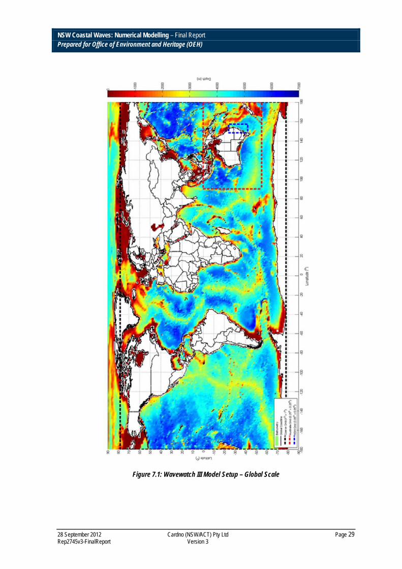
NSW Coastal Waves: Numerical Modelling – Final Report Prepared for Office of Environment and Heritage (OEH)
28 September 2012 Cardno (NSW/ACT) Pty Ltd Page 29 Rep2745v3-FinalReport Version 3
Figure 7.1: Wavewatch III Model Setup – Global Scale
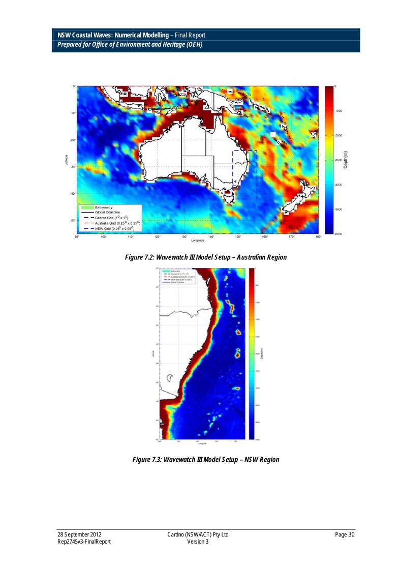
NSW Coastal Waves: Numerical Modelling – Final Report Prepared for Office of Environment and Heritage (OEH)
28 September 2012 Cardno (NSW/ACT) Pty Ltd Page 30 Rep2745v3-FinalReport Version 3
Figure 7.2: Wavewatch III Model Setup – Australian Region
Figure 7.3: Wavewatch III Model Setup – NSW Region

NSW Coastal Waves: Numerical Modelling – Final Report Prepared for Office of Environment and Heritage (OEH)
28 September 2012 Cardno (NSW/ACT) Pty Ltd Page 31 Rep2745v3-FinalReport Version 3
7.1.1 Model Sensitivities
Grid Resolution
The sensitivity of the WW-III model results to grid resolution was tested by running a test case that included a fourth nested grid with a spatial resolution of 0.025o (approx. 2.5km). This test case was then compared to the hindcast that used a spatial grid resolution of 0.05o (approx. 5km). Table 7.1 provides error statistics comparing the differences between the test case (grid resolution = 0.025o) to the hindcast results (grid resolution = 0.05o). The error statistics are averaged over the seven deepwater WRB’s for all wave heights (that is, no Hm0 threshold) for the two month period of June and July 2006. Section 5.8.1 provides a description of the validation metrics utilised in this study. Figure 7.4 presents time-series plots comparing this test case to the hindcast results, whilst also showing the measured wave results. The two WW-III model results essentially over-plot each other.
This result indicates that, for the NSW deepwater Waverider buoy locations, and the CFSR wind field data set which has been adopted in this study, the WW-III model is relatively insensitive to grid resolution better than 5km, and due to the added benefit of computation efficiency, the 5km grid has been deemed the more suitable for this model. If higher resolution wind field data were to be applied to the WW-III model in the future, the sensitivity of the model to grid resolution should be re-considered.
Table 7.1: WW-III Model Error Statistics Comparing a Spatial Grid Resolution of 2.5km to 5km
Parameter Model Skill Bias RMS Scatter Index (%) Correlation, R
Hm0 (m) 1.00 0.03 0.04 1.69% 1.00
Tm01 (sec) 1.00 0.01 0.13 1.85% 0.99
Tp (sec) 0.98 -0.03 0.60 6.52% 0.97
Pk Dir (oTN) 0.98 0.20 9.37 7.07% 0.97

NSW Coastal Waves: Numerical Modelling – Final Report Prepared for Office of Environment and Heritage (OEH)
28 September 2012 Cardno (NSW/ACT) Pty Ltd Page 32 Rep2745v3-FinalReport Version 3
Figure 7.4: WW-III Model Sensitivity at the Sydney Deepwater WRB, Grid Resolution
Bottom Friction
The deepwater physics of the Wavewatch III model system are applicable in most wave conditions up to 30m in water depth, provided that there is enough spatial resolution in the model (Rogers and Campbell, 2009). Therefore, the locations of the NSW deep water WRB’s are in sufficient depth to be resolved by the physics of the WW-III model system. In order to investigate the sensitivity of the WW-III model to bottom friction, a sensitivity simulation with the bottom friction coefficient set at -0.038m2s-3 was modelled. The results from this scenario were then compared with the hindcast case that used a bottom friction coefficient of -0.067m2s-3.
Table 7.2 provides error statistics comparing the differences between this test case (bottom friction coefficient = -0.038m2s-3) and the hindcast results (bottom friction coefficient = -0.067m2s-3). The error statistics are averaged over the seven deepwater WRB’s for all wave heights (that is, no Hm0 threshold) for the two month period of June and July 2006. Figure 7.5 presents time-series plots comparing this test case with the hindcast results, whilst also showing the measured wave results. The two WW-III model results essentially over-plot each other. This result indicates that for the depths of the NSW deepwater Waverider buoys, the WW-III model is extremely insensitive to the bottom friction coefficient used for simulating deep water wave conditions.

NSW Coastal Waves: Numerical Modelling – Final Report Prepared for Office of Environment and Heritage (OEH)
28 September 2012 Cardno (NSW/ACT) Pty Ltd Page 33 Rep2745v3-FinalReport Version 3
Table 7.2: WW-III Model Error Statistics Comparing a Bottom Friction Coefficients of -0.067 and -0.038m2s-3
Parameter Model Skill Bias RMS Scatter Index (%) Correlation, R
Hm0 (m) 1.00 0.00 0.01 0.34% 1.00
Tm01 (sec) 1.00 0.00 0.03 0.42% 1.00
Tp (sec) 1.00 0.01 0.28 3.03% 0.99
Pk Dir (oTN) 1.00 0.12 3.64 2.73% 0.99
Figure 7.5: WW-III Model Sensitivity at Sydney Deepwater WRB, Bottom Friction
7.2 SWAN Transition Model
To make future near-shore SWAN models easy to incorporate into the wave model system, a single transfer SWAN grid covering the NSW coast has been developed in order to couple the WW-III model to the SWAN model system. In doing so, more refined SWAN grids can easily be nested in this transition grid. Figure 7.6 shows the area covered by the SWAN transition grid. This grid has a resolution of 0.025o (approximately 2.5km) and extends from Brisbane in the north to Mallacoota Airport in the south and approximately 10 to 20km offshore to approximately 100m to 150m water depth. The deepwater physics of the Wavewatch III model system are applicable in most wave conditions in 30m water depth, provided that there is enough spatial resolution in the model (Rogers and Campbell, 2009). To minimise potential issues from the difference

NSW Coastal Waves: Numerical Modelling – Final Report Prepared for Office of Environment and Heritage (OEH)
28 September 2012 Cardno (NSW/ACT) Pty Ltd Page 34 Rep2745v3-FinalReport Version 3
in the wave growth physics between the SWAN and Wavewatch III models, the coupling between the two model systems has been undertaken as close to the coast as possible and where the deepwater physics of the Wavewatch-III model are still valid.
Table 7.3 provides a summary of the physical parameter settings used in the SWAN transfer model.
Table 7.3: SWAN Transfer Model Parameter Settings
Model Parameter Setting
Version 40.85
Resolution 0.025deg (≈2.5km)
Time Step 15 min
Max Iterations per time step 15
Percentage of wet grid cells where iterative criteria is satisfied 95%
Number of directional bins 36
Number of frequency bins 24
Frequency bin range 0.05 – 1.0 Hz
Propagation Scheme BSBT
Generation Mode for Physics 3rd Generation
Wind Growth ON
White Capping ON
Quadruplet Wave Interactions
Numerical Procedure 2. Fully explicit computation of nonlinear
transfer with DIA
Lambda (Coefficient for quadruplet configuration) 0.45
Cn14 (Proportionality coefficient for quadruplet configuration)
3x10⁷
Csh1 (Coefficient for shallow water scaling) 5.5
Csh2 (Coefficient for shallow water scaling) 0.833333
Csh3 (Coefficient for shallow water scaling) -1.25
Quadruplet Limiters Ursell 10
Threshold for fraction of breaking waves 1
Wave Breaking Coefficient of the rate of dissipation 1
Ratio of max. individual wave height over depth 0.73
Bottom Friction Formulation JONSWAP
Constant Friction Coefficient 0.038m2s-3
Wave propagation in spectral space
Refraction ON
Frequency Shift ON
Wave Setup (Not available for unstructured grids) OFF
Triad Wave-Wave Interactions OFF
Diffraction OFF
Vegetation OFF
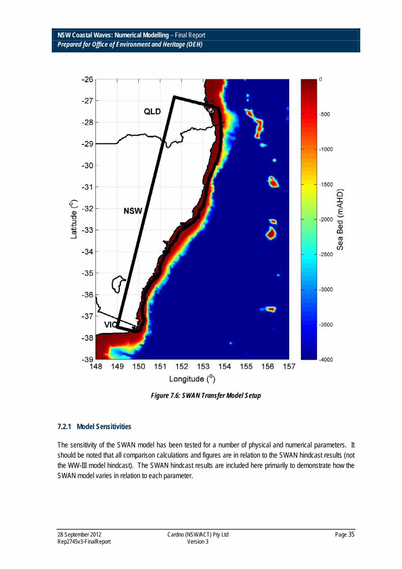
NSW Coastal Waves: Numerical Modelling – Final Report Prepared for Office of Environment and Heritage (OEH)
28 September 2012 Cardno (NSW/ACT) Pty Ltd Page 35 Rep2745v3-FinalReport Version 3
Figure 7.6: SWAN Transfer Model Setup
7.2.1 Model Sensitivities
The sensitivity of the SWAN model has been tested for a number of physical and numerical parameters. It should be noted that all comparison calculations and figures are in relation to the SWAN hindcast results (not the WW-III model hindcast). The SWAN hindcast results are included here primarily to demonstrate how the SWAN model varies in relation to each parameter.

NSW Coastal Waves: Numerical Modelling – Final Report Prepared for Office of Environment and Heritage (OEH)
28 September 2012 Cardno (NSW/ACT) Pty Ltd Page 36 Rep2745v3-FinalReport Version 3
7.2.1.1 Model Physics
Quadruplets
Quadruplets affect the frequency shifting of wave energy – see Section 4.2.1. The default SWAN value of 0.25 for lambda was found to result in wave conditions that were concentrated in the higher frequencies and hence wave periods were underestimated using the default value. The model calibration process found that a lambda value of 0.45 provided the best comparison between the model results and the measured data. Table 7.4 provides error statistics comparing the SWAN default settings for quadruplets (lambda = 0.25) to the hindcast results (lambda = 0.45). The default quadruplets on average had a reduction in mean wave period (Tm01) of approximately 1s compared to the calibrated model (lambda = 0.45). The error statistics are averaged over the seven deepwater WRBs for all wave heights (that is, no Hm0 threshold) for the two month period of June and July 2006.
Table 7.4: SWAN Transition Model Error Statistics Comparing the Default Quadruplets to the Hindcast Model
Parameter Model Skill Bias RMS Scatter Index (%) Correlation, R
Hm0 (m) 0.99 0.10 0.13 4.61% 1.00
Tm01 (sec) 0.87 -0.95 1.07 7.48% 0.95
Tp (sec) 0.96 -0.10 0.96 10.59% 0.92
Peak Dir (oTN) 0.91 3.14 29.15 21.53% 0.84
Figure 7.7 presents a time-series comparison at the Sydney deepwater WRB between the measured, hindcast and default quadruplets (lambda = 0.25) wave results.
Figure 7.7: SWAN Transition Model Sensitivity at Sydney Deepwater WRB, Quadruplets

NSW Coastal Waves: Numerical Modelling – Final Report Prepared for Office of Environment and Heritage (OEH)
28 September 2012 Cardno (NSW/ACT) Pty Ltd Page 37 Rep2745v3-FinalReport Version 3
Wind Growth
Two wind growth models were tested for the SWAN transition model presented in Section 7.2. The Komen model (default) as described in Komen et al. (1994) and the Janssen model described in Janssen (1989, 1991). Calibration runs showed that the Janssen model creates too much sea as can be seen in the error statistics in Table 7.5, and the time-series plot in Figure 7.8, which clearly indicates that the Janssen model significantly overestimates the wave conditions compared to the measured data. The error statistics are averaged over the seven deepwater WRBs for all wave heights (that is, no Hm0 threshold) for the two month period of June and July 2006.
Table 7.5: SWAN Transfer Model Error Statistics Comparing the Janssen Wind Growth Model to the Hindcast Model (Komen Wind Growth Model)
Parameter Model Skill Bias RMS Scatter Index (%) Correlation, R
Hm0 (m) 0.64 1.32 1.77 62.33% 0.79
Tm01 (sec) 0.78 -0.66 1.13 14.32% 0.76
Tp (sec) 0.52 -1.47 2.77 25.94% 0.44
Pk Dir (oTN) 0.54 10.91 70.00 47.76% 0.44
Figure 7.7: Transition Model Sensitivity at Sydney Deepwater WRB, Wind Growth Model

NSW Coastal Waves: Numerical Modelling – Final Report Prepared for Office of Environment and Heritage (OEH)
28 September 2012 Cardno (NSW/ACT) Pty Ltd Page 38 Rep2745v3-FinalReport Version 3
Bottom Friction
The bottom friction coefficient in the SWAN transition model was tested for the lower and upper bounds of the JONSWAP bottom friction coefficient. A value of 0.038m2s-3 is generally used for swell conditions and 0.067m2s-3 is generally used for wind sea conditions. The hindcast model uses a bottom friction coefficient value of 0.038m2s-3. The model is quite insensitive to the bottom friction coefficient as can be seen in Table 7.6 and Figure 7.9 at the deepwater Waverider buoy locations. The error statistics are averaged over the seven deepwater WRBs for all wave heights (that is, no Hm0 threshold) for the two month period of June and July 2006.
Bottom friction for near shore SWAN model wave conditions in 10m to 15m water depth has been investigated using the Newcastle SWAN model – see Section 7.3.1.1.
Table 7.6: SWAN Transfer Model Error Statistics Comparing Bottom Friction Coefficients
Parameter Model Skill Bias RMS Scatter Index (%) Correlation, R
Hm0 (m) 1.00 0.00 0.01 0.31% 1.00
Tm01 (sec) 1.00 0.00 0.04 0.60% 1.00
Tp (sec) 1.00 0.00 0.23 2.59% 1.00
Peak Dir (oTN) 0.99 -0.08 7.91 5.92% 0.99
Figure 7.8: SWAN Transition Model Sensitivity at Sydney Deepwater WRB, Bottom Friction

NSW Coastal Waves: Numerical Modelling – Final Report Prepared for Office of Environment and Heritage (OEH)
28 September 2012 Cardno (NSW/ACT) Pty Ltd Page 39 Rep2745v3-FinalReport Version 3
7.2.1.2 Numerics
Frequency Discretization
The sensitivity of the SWAN model to changes in the frequency bin size and range has also been tested. The default value of the highest frequency range is 1.0Hz with a total of 24 frequency bins. The SWAN model applied in this study also adopts this default value. A sensitivity case was setup with the highest frequency limited to 0.5Hz and a corresponding increase in the resolution of the model in the high frequency end of the spectrum. A hindcast study undertaken by the UK Met Office using the SWAN wave model system had indicated that this was a way to improve the frequency calibration of the SWAN model (Bunney, 2011). By changing the high frequency limit and keeping the same number of frequency bins, the distribution of the frequency bins is changed and there is more frequency resolution across the mid-frequency range of the spectrum. The test case shows that only small differences in Hm0 and Tm01 were noticeable for ambient wave conditions. By reducing the highest frequency from 1.0 to 0.5Hz, the ambient wave heights were generally slightly larger, and Tm01 was slightly shorter.
Table 7.7 provides error statistics comparing the 0.5Hz upper frequency limit to the hindcast results, wherein the upper frequency bin is limited to 1.0Hz. The error statistics have been averaged over the seven deepwater WRBs for all wave heights (that is, no Hm0 threshold) for the two month period of June and July 2006. Figure 7.10 shows a time-series comparison of wave results at the Sydney deepwater WRB between the measured, hindcast and the test case where the highest frequency is set at 0.5Hz.
Table 7.7: SWAN Transfer Model Error Statistics Comparing Wave Results for Different Frequency Bin Discretizations
Parameter Model Skill Bias RMS Scatter Index (%) Correlation, R
Hm0 (m) 1.00 0.07 0.11 4.27% 1.00
Tm01 (sec) 0.96 -0.24 0.52 7.29% 0.95
Tp (sec) 0.93 -0.11 1.21 13.29% 0.88
Peak Dir (oTN) 0.96 1.36 18.23 13.52% 0.93

NSW Coastal Waves: Numerical Modelling – Final Report Prepared for Office of Environment and Heritage (OEH)
28 September 2012 Cardno (NSW/ACT) Pty Ltd Page 40 Rep2745v3-FinalReport Version 3
Figure 7.9: SWAN Transition Model Sensitivity at Sydney Deepwater WRB, Frequency Bin
7.2.1.3 WW-III and SWAN Coupling
Originally, when analysing the SWAN model results (compared to WW-III) from a preliminary model set-up, it became apparent that there were fundamental differences between the results from the two models that appeared to be related to the differences in the wind growth physics of the two model. The differences between the models are most apparent in the SWAN model when the wind is blowing offshore or towards the SWAN boundary. In such wind conditions, the wave conditions (in particular the wave period), calculated by SWAN are quite dissimilar to those of the WW-III model. Figure 7.11 illustrates the initial SWAN model grid and the hindcast mean wave period at 00:00 on 3/01/2006. At this time step, the winds are blowing offshore (westerly) along the southern and central regions of the NSW coast. As a result, the wave conditions calculated by SWAN generated over the relatively large fetch from the coastline to the eastern edge of the model which couples to the WW-III model are quite different to the boundary conditions provided by WW-III on the boundary of the SWAN model. This is illustrated in Figure 7.11 by the significant jump in wave period at the seaward model boundary from Crowdy Head to Eden. The boundary points show the conditions being input from the WW-III model, whilst the results within the domain are calculated by SWAN from winds which are generally opposing the swell wave direction. The wave spectra from the SWAN model appears to differ

NSW Coastal Waves: Numerical Modelling – Final Report Prepared for Office of Environment and Heritage (OEH)
28 September 2012 Cardno (NSW/ACT) Pty Ltd Page 41 Rep2745v3-FinalReport Version 3
significantly from the WW-III model when the local wind conditions along the coastline are opposing the dominant direction of the swell wave conditions.
Figure 7.10: Original SWAN Transition Grid, Tm01 at 03/01/2006 00:00:00
Figure 7.12 shows a different time-step from the initial SWAN model when there are generally onshore (north-easterly winds). Here the wave periods in the SWAN model match up quite well with the WW-III boundary conditions between Crowdy Head and Eden. In this time step, the SWAN model hasn’t been able to influence the wave conditions near the boundary as much because any new wave energy from wind growth over the SWAN model is heading towards the coastline in a similar direction to the boundary wave conditions from the WW-III model.

NSW Coastal Waves: Numerical Modelling – Final Report Prepared for Office of Environment and Heritage (OEH)
28 September 2012 Cardno (NSW/ACT) Pty Ltd Page 42 Rep2745v3-FinalReport Version 3
Figure 7.11: Original SWAN Transition Grid, Tm01 at 16/01/2006 12:00:00
Figures 7.13 and 7.14 show the transition SWAN model grid that has been applied in this study for time-steps the same as those shown in Figures 7.11 and 7.12. By reducing the extent of the SWAN transition grid, the fetch lengths within the SWAN model have been significantly reduced and the effect of the differences in the SWAN and WW-III wind growth physics have been minimised. In doing so, the WW-III model results are being applied much closer to the coastline and the model system is maximising the use of the WW-III model results, which appear to be significantly more accurate in the description of the frequency spectrum.
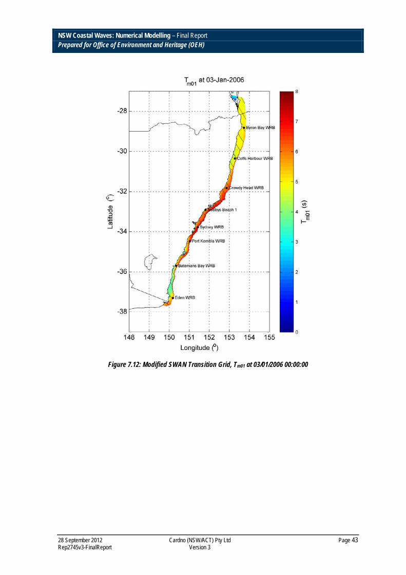
NSW Coastal Waves: Numerical Modelling – Final Report Prepared for Office of Environment and Heritage (OEH)
28 September 2012 Cardno (NSW/ACT) Pty Ltd Page 43 Rep2745v3-FinalReport Version 3
Figure 7.12: Modified SWAN Transition Grid, Tm01 at 03/01/2006 00:00:00

NSW Coastal Waves: Numerical Modelling – Final Report Prepared for Office of Environment and Heritage (OEH)
28 September 2012 Cardno (NSW/ACT) Pty Ltd Page 44 Rep2745v3-FinalReport Version 3
Figure 7.13: Modified SWAN Transition Grid, Tm01 at 16/01/2006 12:00:00
7.3 Inshore SWAN Models
This project has developed two near shore coastal SWAN models to undertake inshore validation of the wave model system. The two sites selected for this exercise were Port Kembla and Newcastle. Port Kembla was initially selected because of the presence of an inshore wave measurement data set from the channel at the entrance to Port Kembla. PKPC operate a real-time ADCP current and wave measurement system in approximately 19m depth of water. During the model calibration process it became evident that although the calibration of the model system to the deepwater Port Kembla WRB data set was very good, the agreement of the model to the measured inshore data set was poor and the model system consistently had wave heights 30 to 40% larger than those in the data set. Further inspection of the wave data and consideration of the configuration of the ADCP system indicated that the measured data set is likely to significantly underestimate the shorter period wave energy (T<6s) because the system is designed to focus on measuring swell wave conditions (T>7s) which affect the operations of PKPC.

NSW Coastal Waves: Numerical Modelling – Final Report Prepared for Office of Environment and Heritage (OEH)
28 September 2012 Cardno (NSW/ACT) Pty Ltd Page 45 Rep2745v3-FinalReport Version 3
As a result of the limitations in comparing the sea and swell wave conditions simulated by the wave model with the swell dominated data set at Port Kembla, the inshore calibration of the model system focused on Newcastle where NPC operate two WRBs near the entrance to the Hunter River as part of their SAUCS operational system – see Section 5. These instruments have measured data since 2006 and are the same types of instrument as those used to measure the deepwater wave data along the NSW coastline.
An unstructured SWAN model grid has been developed for the Newcastle coastline. It extends from The Entrance in the south to Hawks Nest in the north and approximately 20 to 25km offshore. The model resolution varies from 1500m near the SWAN model boundaries to 40m inside the 15m depth contour around Newcastle (near the WRBs). Figure 7.15 presents a plan view of the model bathymetry at the entrance to Newcastle Harbour and the location of the near shore WRBs. Table 7.8 provides a summary of the physical parameter settings used in the SWAN Newcastle inshore model.
Figure 7.14: Inshore Newcastle SWAN Model Bathymetry

NSW Coastal Waves: Numerical Modelling – Final Report Prepared for Office of Environment and Heritage (OEH)
28 September 2012 Cardno (NSW/ACT) Pty Ltd Page 46 Rep2745v3-FinalReport Version 3
Table 7.8: SWAN Newcastle Inshore Model Parameter Settings
Model Parameter Setting
Version 40.85
Resolution 40 – 1500m
Time Step 15 min
Max Iterations per time step 15
Percentage of wet grid cells where iterative criteria is satisfied 95%
Number of directional bins 36
Number of frequency bins 24
Frequency bin range 0.05 – 1.0 Hz
Propagation Scheme BSBT
Generation Mode for Physics 3rd Generation
Wind Growth ON
White Capping ON
Quadruplet Wave Interactions
Numerical Procedure 2. Fully explicit computation of nonlinear
transfer with DIA
Lambda (Coefficient for quadruplet configuration) 0.45
Cn14 (Proportionality coefficient for quadruplet configuration)
3x10⁷
Csh1 (Coefficient for shallow water scaling) 5.5
Csh2 (Coefficient for shallow water scaling) 0.833333
Csh3 (Coefficient for shallow water scaling) -1.25
Quadruplet Limiters Ursell 10
Threshold for fraction of breaking waves 1
Wave Breaking Coefficient of the rate of dissipation 1
Ratio of max. individual wave height over depth 0.73
Bottom Friction Formulation JONSWAP
Constant Friction Coefficient 0.038m2s-3
Wave propagation in spectral space
Refraction ON
Frequency Shift ON
Wave Setup (Not available for unstructured grids) OFF
Triad Wave-Wave Interactions OFF
Diffraction OFF
Vegetation OFF

NSW Coastal Waves: Numerical Modelling – Final Report Prepared for Office of Environment and Heritage (OEH)
28 September 2012 Cardno (NSW/ACT) Pty Ltd Page 47 Rep2745v3-FinalReport Version 3
7.3.1 Model Sensitivities – Newcastle Near Shore SWAN Model
7.3.1.1 Model Physics
Bottom Friction
The SWAN inshore model sensitivity was investigated in terms of the lower and upper bounds of the JONSWAP bottom friction coefficient. A value of 0.038m2s-3 is generally used for swell conditions and 0.067m2s-3 is generally used for wind sea conditions. The Newcastle SWAN hindcast model uses a bottom friction coefficient value of 0.038m2s-3. The Newcastle model is quite insensitive to the bottom friction coefficient at the depths of the near shore Waverider buoys, as can be seen in Table 7.9 and Figure 7.16. The error statistics are averaged over the two inshore WRBs at Newcastle for all wave heights (that is, no Hm0 threshold) for the two month period of June and July 2006.
Table 7.9: SWAN Transfer Model Error Statistics Comparing the Bottom Friction Coefficients for the Inshore Newcastle Grid
Parameter Model Skill Bias RMS Scatter Index (%) Correlation, R
Hm0 (m) 1.00 0.00 0.01 0.48% 1.00
Tm01 (sec) 1.00 -0.02 0.03 0.41% 1.00
Tp (sec) 0.99 -0.02 0.50 5.47% 0.98
Peak Dir (oTN) 1.00 -0.05 4.56 3.17% 0.99
Figure 7.15: SWAN Transition Model Sensitivity at Nobbys Beach 2 WRB, Bottom Friction Coefficient
NSW Coastal Waves: Numerical Modelling – Final Report Prepared for Office of Environment and Heritage (OEH)
28 September 2012 Cardno (NSW/ACT) Pty Ltd Page 48 Rep2745v3-FinalReport Version 3
8 VALIDATION OF WIND FIELD DATA
Section 6 described the three global scale hindcast wind data sets that Cardno has considered to provide the boundary forcing for the NSW wave modelling system. The following sections describe the outcomes from the wind data validation process adopted in this project.
8.1 Coastal Wind Measurements
Examination of the comparison between hindcast and measured wind data from the coastal wind sites indicated that the complexity of comparing modelled ‘over-water’ wind conditions with measured data from land locations was significant, even, when the winds were blowing from offshore and there was very little obstruction to the winds between the coastline and the measurement site. Due to this complexity, and the difficulty of adjusting the overland measurements to be representative of ‘over-water’ winds, which was identified in progress reports, the project did not focus on validating hindcast winds to measured wind data sets from over-land sites.
Based on the initial wind and wave model calibration exercises, the GDAS winds were excluded from detailed investigations because they proved to be significantly inferior to the CCMP and CFSR winds in the 2006 calibration period. The GDAS winds are noticeably poor in the near shore region and are unable to resolve spatially varying winds on a local scale due to the coarse resolution of the GDAS winds.
8.2 Literature Review of Hindcast Wind Data Sets
As part of assessing the most suitable hindcast wind data set for the OEH wave model system, a literature review was undertaken of global scale hindcast wind data sets that have been applied in wave hindcast studies. Discussions were also held with Dr Jose-Henrique Alves from the SGR team at the US National Weather Service. Currently the SGR team is leading the further development of the Wavewatch-III model system for US government agencies. This review process identified the following outcomes:-
CFSR or CFSRR hindcast winds is the wind forcing data set that is now generally adopted by NOAA and the NWS in the United States. Currently a 30-years hindcast project run by NOAA and the NWS is adopting the CFSR data set (Chawla et al, 2011).
The CFSR data has been compared against earlier re-analysis data sets and has demonstrated significant improvement in the accuracy of ocean surface wind fields (Cardone et al, 2011).
A major issue with the CCMP wind data set, is that, although it can be highly accurate at times, the quality and potential bias of the data set can vary over time due to a number of factors, including:-
o Availability of satellite scatterometer data;
o Changes to the satellite systems that provide the scatterometer data - for example, the data quality for the QuickSCAT satellite, which was operational from1999 to 2009, differs from data collected before or after that time;

NSW Coastal Waves: Numerical Modelling – Final Report Prepared for Office of Environment and Heritage (OEH)
28 September 2012 Cardno (NSW/ACT) Pty Ltd Page 49 Rep2745v3-FinalReport Version 3
o The time interval of the CCMP data set is 6-hours, compared to 1-hour for the CFSR data sets, which may mean that the CCMP data is more likely to miss storm peaks; and
o Quality and capture of scatterometer data is affected by atmospheric conditions, for example rainfall.
Based on several, long wave-hindcast studies in which Cardno has been involved at a number of locations, including the Gulf of PNG, northwest Australia and in Bass Strait, the potential long term bias of the CCMP winds is a concern Generally this data set will only provide 10 to 12-years of reliable hindcast wind data. A key benefit of the CFSR wind data set is that since it is obtained from a calibrated global atmospheric model over a 20-to-30 year hindcast period, the data set is likely to have less bias from technological developments in scatterometer data compared with the CCMP data set.
As a result of the background research and discussion with members of the research community, the CFSR data set has been identified as the preferred long duration global hindcast wind data set for the OEH wave model system. The following sections present some validation of the CFSR wind data.
8.3 Yolla (Origin Energy Data Set)
The hindcast wind data sets have been compared to wind measurements from the Yolla platform in Bass Strait – see Figure 6.1. Whilst this site is not on the NSW coastline, this data set, which was made available by Origin Energy, is a true ‘over-water’ wind data set and the Yolla site is affected by many of the same weather systems that affect the southern NSW coastline.
Wind data have been recorded at Yolla since 20 April 2009. The data recorded are one minute averages from two anemometers mounted on the crane at 43m above mean sea level. For comparison with winds used in the wave modelling, these measured values need to be adjusted to 10 minute averages at 10m above mean sea level using the procedures outlined in USACE (2002). The data from 25 October 2009 to 31 December 2009 have been used for comparison with the hindcast wind data sets.
Figures 8.1 to 8.4 present validation plots using measured winds from Yolla. The figures are:-
Figure 8.1: time series plots of 1-month – modelled and measured.
Figure 8.2: QQ plot based on 3-months of data.
Figure 8.3: scatter plots (modelled and measured) from a 3-month period.
Figure 8.4: percentage occurrence of winds from section directional sectors (modelled and measured).
The QQ plot presented in Figure 8.2 appears similar to a traditional X-Y scatter plot; however, a QQ-plot compares two data sets on a probability basis. This means that, unlike a normal X-Y scatter plot, the data presented on a QQ-plot is not coincident in time.
The comparison analyses indicate that the CFSR winds agree well with the measured data. The CFSR winds are slightly positively biased at higher wind speeds and there are some differences in the directional

NSW Coastal Waves: Numerical Modelling – Final Report Prepared for Office of Environment and Heritage (OEH)
28 September 2012 Cardno (NSW/ACT) Pty Ltd Page 50 Rep2745v3-FinalReport Version 3
distribution compared to the measured data. However, the CSFR data describe the general wind direction distribution well.
8.4 Comparison between CCMP and CFSR Wind Forcing for the WW-III Model
Due to the limitations in available data for validating the ‘over-water’ winds from the available hindcast data sets, during the development of the OEH wave model, a one-year hindcast using both the CCMP and CFSR wind data sets to force the WW-III model was undertaken to compare the hindcast wave conditions at each of the NSW deepwater Waverider buoy locations. Figure 8.5 presents a series of comparisons from the Sydney (Longreef) deepwater WRB for the 2006 hindcast period based on applying the CFSR wind fields. Figure 8.6 presents a similar set of comparison plots based on applying the CCMP winds to the WW-III model system. For the hindcast model simulations presented in Figures 8.5 and 8.6, no adjustment to the near-coast CFSR or CCMP wind fields was applied.
The quantitative validation metrics for wave height and period that are displayed in Figures 8.5 and 8.6 indicate that the agreement between measured and both sets of hindcast data is similar, although the CFSR hindcast has marginally better validation metrics, which are identified by a higher R2 coefficient and a smaller scatter index. This outcome supports the adoption of the CFSR data set as the source of hindcast wind forcing for the OEH model.
Figures 8.5 and 8.6 indicate that both the CFSR and CCMP hindcast wave heights tend to be biased towards under-prediction of the largest storm wave heights observed in 2006. The improvement of the WW-III model performance following the adoption of a near-coast wind adjustment algorithm is presented in Section 8.5.
Figure 8.5: Comparison of Hindcast Waves with CFSR wind forcing and Measured Waverider Buoy Data at Sydney – 2006

NSW Coastal Waves: Numerical Modelling – Final Report Prepared for Office of Environment and Heritage (OEH)
28 September 2012 Cardno (NSW/ACT) Pty Ltd Page 51 Rep2745v3-FinalReport Version 3
Figure 8.6: Comparison of Hindcast Waves with CCMP Wind Forcing and Measured Waverider Buoy Data at Sydney – 2006
The CFSR wind database has been selected as the most suitable wind database to use in the wave model. It has a much better temporal resolution (hourly) than the CCMP wind database (6-hourly) and therefore is able to define the shorter duration storms better, as well as resolving storm peaks more accurately. It is also more consistent through time and does not depend on scatterometer data.
8.5 QuickSCAT Scatterometer Data
From the outputs of the initial wave model simulations, it was evident that the NSW wave model appeared to be describing deepwater wave heights, perhaps 100km offshore of the coastline, realistically. However, closer to the coast, even though the water depth is still relatively deep, and there has been little to no transformation or energy loss due to the coastal bathymetry, the model system was indicating that the wave heights were consistently lower than measured at the deepwater WRB locations.
Analyses of wind maps have shown that all three wind databases demonstrate decreasing wind speeds in the near shore region when compared to the equivalent offshore region. In order to assess this trend within the data sets, the CCMP and CFSR winds were analysed in more detail for the near shore and offshore regions. The hindcast wind data sets have been compared to estimates of wind speed and direction available from the QuickSCAT scatterometer data set which was collected by NOAA using an earth-observing satellite between 1999 and 2009. Details on the QuickSCAT mission can be found at:- http://winds.jpl.nasa.gov/missions/quikscat/index.cfm.
Figures 8.7 to 8.10 present comparisons between scatterometer (QuickSCAT) wind data and the CCMP and CFSR winds for a near shore area and an area centred approximately 100km offshore of Sydney (Figures 8.7

NSW Coastal Waves: Numerical Modelling – Final Report Prepared for Office of Environment and Heritage (OEH)
28 September 2012 Cardno (NSW/ACT) Pty Ltd Page 52 Rep2745v3-FinalReport Version 3
and 8.8), and Byron Bay (Figures 8.9 and 8.10). Comparisons have been carried out for a number of storms at Byron Bay, Sydney and Eden. The results indicate that the CCMP and CFSR winds always show smaller near shore wind speeds than their equivalent, further offshore locations. On the other hand, the scatterometer data suggests that at times the near shore wind speeds were in fact higher than the offshore wind speeds. At Byron Bay, it appears that the scatterometer data shows larger wind speeds near shore compared to offshore for all the analysed storms. Near Sydney, the scatterometer data shows more variability, with about half the storms recording scatterometer winds stronger near shore than offshore. At Eden, the scatterometer offshore wind speeds are mostly (but not always), larger than the near shore wind speeds.
Wind profiles (CFSR and CCMP) have also been analysed extending from the coastline to approximately 150km offshore at two locations; south of Sydney and Nobby’s Beach. Winds during the top ten storms for 2006 were analysed south of Sydney, whilst the top eight storms were analysed at Nobby’s Beach. Figures 8.11 and 8.12 show typical results of these wind profile analyses in the near shore region. Within approximately 100km of the coastline the figures show that the wind speeds decrease as they approach the coastline. This trend is present for all the events analysed.
Figure 8.13 shows time-series plots which include two adjusted wind data sets at Byron Bay for June/July 2006. CFSR-3 refers to the original winds including air-sea temperature difference, CFSR-4 refers to the factored winds, whilst CFSR-5 refers to a case where the 100km offshore winds are applied up to the coastline.
Figures 8.14 to 8.20 compare the WW-III wave results from the raw CFSR winds (CFSR-3) and the factored CFSR (CFSR-4) winds to the measured wave data at the seven deepwater WRB locations. At all sites the factored CFSR wind simulation describes the peak storm wave heights better.
In order to validate the near-coast wind adjustment scheme, a comparison between hindcast and measured peak storm wave heights during the year-2006 was undertaken. The comparison was undertaken with the WW-III model forced by the raw, unadjusted CFSR, and also the adjusted CFSR winds described above (CFSR-4).
For the 2006 hindcast period, Table 8.1 compares the relative error range for peak storm wave height at all the deepwater Waverider buoy sites for events where Hm0 exceeded 2.5m. Table 8.1 indicates that the adjustment to the near-coast wind speed has significantly improved the performance of the OEH wave model, although based on Table 8.1, the model is still biased to under-estimating peak storm wave heights.

LJ2949/R2745 September 2012J:\CM\LJ2949−WWIIIModel−DECCW\Transmittal−ToClient\28092012-FinalReport\Figures
NSW Coastal Waves Numerical Modelling
CFSR Wind Validation −Yolla PlatformWind Speed and Direction (25/Oct/09 − 25/Nov/09)
Figure 8.1

LJ2949/R2745 September 2012J:\CM\LJ2949−WWIIIModel−DECCW\Transmittal−ToClient\27022012−DraftReport\Figures
NSW Coastal Waves Numerical Modelling
CFSR Wind Validation −Yolla PlatformQ−Q Plot − Wind Speed
Figure 8.2

LJ2949/R2745 September 2012J:\CM\LJ2949−WWIIIModel−DECCW\Transmittal−ToClient\28092012-FinalReport\Figures
NSW Coastal Waves Numerical Modelling
CFSR Wind Validation −Yolla PlatformWind Speed and Direction Scatter Plots
Figure 8.3

LJ2949/R2745 September 2012J:\CM\LJ2949−WWIIIModel−DECCW\Transmittal−ToClient\28092012-FinalReport\Figures
NSW Coastal Waves Numerical Modelling
CFSR Wind Validation −Yolla PlatformVariation in Percentage Occurance per Directional Sector
Figure 8.4

LJ2949/R2745 September 2012J:\CM\LJ2949−WWIIIModel−DECCW\Transmittal−ToClient\28092012-FinalReport\Figures
NSW Coastal Waves Numerical Modelling
Wind Speed Comparison in Nearshore and Offshore − SydneyCCMP Vs QuickScat Scatterometry
Figure 8.7
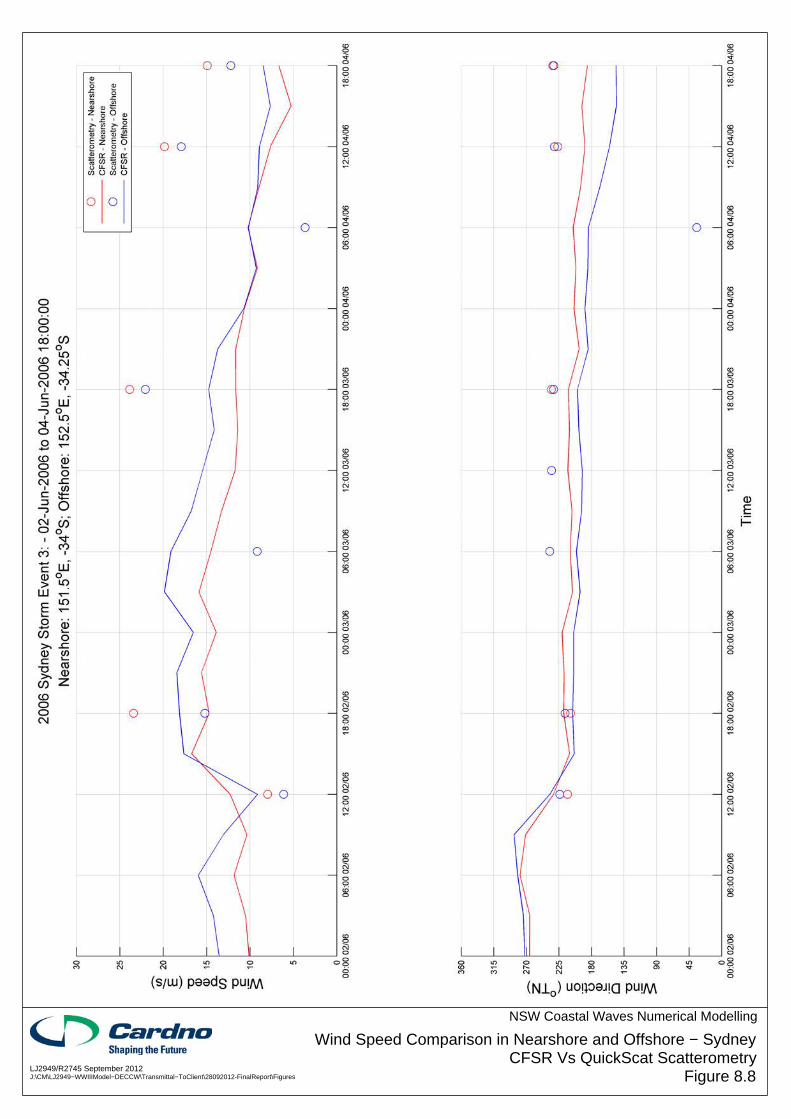
LJ2949/R2745 September 2012J:\CM\LJ2949−WWIIIModel−DECCW\Transmittal−ToClient\28092012-FinalReport\Figures
NSW Coastal Waves Numerical Modelling
Wind Speed Comparison in Nearshore and Offshore − SydneyCFSR Vs QuickScat Scatterometry
Figure 8.8

LJ2949/R2745 September 2012J:\CM\LJ2949−WWIIIModel−DECCW\Transmittal−ToClient\28092012-FinalReport\Figures
NSW Coastal Waves Numerical Modelling
Wind Speed Comparison in Nearshore and Offshore − Byron BayCCMP Vs QuickScat Scatterometry
Figure 8.9

LJ2949/R2745 September 2012J:\CM\LJ2949−WWIIIModel−DECCW\Transmittal−ToClient\28092012-FinalReport\Figures
NSW Coastal Waves Numerical Modelling
Wind Speed Comparison in Nearshore and Offshore − Byron BayCFSR Vs QuickScat Scatterometry
Figure 8.10

LJ2949/R2745 September 2012J:\CM\LJ2949−WWIIIModel−DECCW\Transmittal−ToClient\28092012-FinalReport\Figures
NSW Coastal Waves Numerical Modelling
Offshore Wind Profile − Sydney RegionCCMP and CFSR
Figure 8.11

LJ2949/R2745 September 2012J:\CM\LJ2949−WWIIIModel−DECCW\Transmittal−ToClient\28092012-FinalReport\Figures
NSW Coastal Waves Numerical Modelling
Offshore Wind Profile − Nobbys BeachCCMP and CFSR
Figure 8.12

LJ2949/R2745 September 2012J:\CM\LJ2949−WWIIIModel−DECCW\Transmittal−ToClient\28092012-FinalReport\Figures
NSW Coastal Waves Numerical Modelling
WaveWatch−III Calibration − Byron Bay (June/July 2006)Comparison of Factored and Unfactored CFSR Winds
Figure 8.13

LJ2949/R2745 September 2012J:\CM\LJ2949−WWIIIModel−DECCW\Transmittal−ToClient\28092012-FinalReport\Figures
NSW Coastal Waves Numerical Modelling
WaveWatch−III Calibration − Byron Bay (2006)Measured v CFSR v CFSR−Factored
Figure 8.14

LJ2949/R2745 September 2012J:\CM\LJ2949−WWIIIModel−DECCW\Transmittal−ToClient\28092012-FinalReport\Figures
NSW Coastal Waves Numerical Modelling
WaveWatch−III Calibration −Coffs Harbour (2006)Measured v CFSR v CFSR−Factored
Figure 8.15

LJ2949/R2745 September 2012J:\CM\LJ2949−WWIIIModel−DECCW\Transmittal−ToClient\28092012-FinalReport\Figures
NSW Coastal Waves Numerical Modelling
WaveWatch−III Calibration − Crowdy Head (2006)Measured v CFSR v CFSR−Factored
Figure 8.16

LJ2949/R2745 September 2012J:\CM\LJ2949−WWIIIModel−DECCW\Transmittal−ToClient\28092012-FinalReport\Figures
NSW Coastal Waves Numerical Modelling
WaveWatch−III Calibration − Sydney (2006)Measured v CFSR v CFSR−Factored
Figure 8.17

LJ2949/R2745 September 2012J:\CM\LJ2949−WWIIIModel−DECCW\Transmittal−ToClient\28092012-FinalReport\Figures
NSW Coastal Waves Numerical Modelling
WaveWatch−III Calibration − Port Kembla (2006)Measured v CFSR v CFSR−Factored
Figure 8.18

LJ2949/R2745 September 2012J:\CM\LJ2949−WWIIIModel−DECCW\Transmittal−ToClient\28092012-FinalReport\Figures
NSW Coastal Waves Numerical Modelling
WaveWatch−III Calibration − Batemans Bay (2006)Measured v CFSR v CFSR−Factored
Figure 8.19

LJ2949/R2745 September 2012J:\CM\LJ2949−WWIIIModel−DECCW\Transmittal−ToClient\28092012-FinalReport\Figures
NSW Coastal Waves Numerical Modelling
WaveWatch−III Calibration − Eden (2006)Measured v CFSR v CFSR−Factored
Figure 8.20

LJ2949/R2745 September 2012J:\CM\LJ2949−WWIIIModel−DECCW\Transmittal−ToClient\28092012-FinalReport\Figures
NSW Coastal Waves Numerical Modelling
Near−Coast Wind Adjustment Factors
Figure 8.21

NSW Coastal Waves: Numerical Modelling – Final Report Prepared for Office of Environment and Heritage (OEH)
28 September 2012 Cardno (NSW/ACT) Pty Ltd Page 53 Rep2745v3-FinalReport Version 3
Table 8.1: Summary of Relative Error (%) of Modelled Peak Hm0 (Hm0>2.5m) Compared to the Measured WRB Data – CFSR (unadjusted) and CFSR (adjusted) Wind Forcing
Location No. Of Events
CFSR - Unadjusted CFSR – Near-Coast Wind
Magnitude Adjusted
Minimum Maximum Average Minimum Maximum Average
Byron Bay 25 -44.4% 26.0% -17.2% -28.1% 51.9% -1.2%
Coffs Harbour 31 -49.8% 16.2% -20.3% -38.7% 33.0% -9.8%
Crowdy Head 24 -29.4% 35.7% -8.6% -21.0% 43.6% -1.5%
Sydney 46 -47.6% 22.1% -21.7% -37.4% 28.7% -11.3%
Port Kembla 46 -68.8% 17.6% -26.3% -65.6% 27.8% -12.7%
Bateman’s Bay 25 -52.7% -1.8% -33.5% -45.3% 13.7% -21.3%
Eden 44 -50.0% 55.6% -17.6% -56.0% -48.7% -6.5%
Average -20.7% Average -9.2%
8.6 Near-Coast Wind Adjustment Routine
Based on the outcomes presented in Section 8.5, an adjustment to the near shore wind magnitude has been undertaken. The profiles presented in Section 8.5 were used to calculate mean factors of the wind speeds in the near shore region extending to approximately 100km offshore. These factors were then used to create a factor matrix in order to compensate for the near shore deficiencies in the two wind models. The factor matrix consists of increases ranging from 5% to 20%. From 60km to approximately 100km offshore, wind speeds are increased by 5%, between 30km and 60km offshore wind speeds are increased by 10% and within 30km of the coastline wind speeds are increased by 20%. The factored winds cover the NSW coast and extend in the north to Fraser Island and in the south to Lake Tyers Beach in Victoria. Figure 8.21 indicates the regions where the winds have been factored. Winds have been factored for magnitude only and there are no changes in direction. It should be noted that the Yolla platform site (see Figure 6.1), where the validation of the over-water wind conditions presented in Section 8.2 was undertaken, is located outside the region of wind adjustment.

NSW Coastal Waves: Numerical Modelling – Final Report Prepared for Office of Environment and Heritage (OEH)
28 September 2012 Cardno (NSW/ACT) Pty Ltd Page 73 Rep2745v3-FinalReport Version 3
9 CALIBRATION OF THE WAVE MODEL SYSTEM
9.1 WW-III Model Benchmark Exercise
As described in Section 3.1, a model benchmarking exercise was undertaken to verify that the WW-III model system implemented for this project was consistent with other operational WW-III model systems. The benchmark test for the NSW coast WW-III model was undertaken for a one-month period during May 2009 when an East Coast Low (ECL) storm formed off the north coast of NSW coast and generated large waves from Crowdy Head to Byron Bay. The WW-III model implemented for this project was compared to outputs from the coarser scale NOAA WW-III model.
Figure 9.1 presents a global plan-view plot of significant wave height (Hm0) from the NOAA WW-III model using the GDAS wind field data. Figure 9.2 presents a similar global plan-view plot of significant wave height (Hm0) from the OEH WW-III model using the GDAS wind field data. Both WW-III models produce similar global scale wave height outputs.
Since the OEH WW-III model has nested grids including a 0.25O resolution Australian grid, the results calculated within the Australian scale nested grid are more refined then in the global scale model. As a consequence, some small discrepancies between the Australian and global scale models can be seen along the eastern nested boundary at 180oE in Figure 9.2. Overall, the OEH WW-III model global wave height output agrees well with the NOAA model. This outcome provides confidence that the OEH Wavewatch-III model is consistent with the NOAA system.
Figure 9.1: NOAA WW-III Model (GDAS Winds): Significant Wave Height at 22/05/2009 00:00:00

NSW Coastal Waves: Numerical Modelling – Final Report Prepared for Office of Environment and Heritage (OEH)
28 September 2012 Cardno (NSW/ACT) Pty Ltd Page 74 Rep2745v3-FinalReport Version 3
Figure 9.2: OEH WW-III Model (GDAS Winds): Significant Wave Height at 22/05/2009 00:00:00
9.2 Model Validation using Deepwater Waverider Buoy Data
9.2.1 WW-III Model System
Section 7 presented a discussion on the sensitivity of the WW-III and SWAN models to various model parameter coefficients and the coupling of the WW-III and SWAN model systems. Based on the model set-up for the model systems presented in Section 7, and the adjusted CFSR hindcast wind fields described in Section 9.4, a comprehensive model validation process was undertaken for the year of-2006. The year of 2006 produced the largest number of individual storm peaks (Hm0>4m) along the whole NSW coast based on all of the deepwater Waverider buoy data.
Due to the high-resolution of the WW-III model developed in this project (≈5km resolution), it is appropriate to directly compare the modelled wave conditions from the WW-III model with the measured wave conditions from the deepwater wave buoy data. The output from the SWAN transition model can also be compared to the deepwater wave buoy data. The SWAN model has a higher grid resolution (≈2.5km resolution) and the coupling between the SWAN and WW-III model occurs at a depth of approximately 100m to 150m.
Appendix B presents time-series of modelled (WW-III) and measured deepwater wave parameters during 2006 (Hm0, Tp, Tm01, Dir-Peak). There is generally good correlation and agreement between modelled and measured wave conditions. Whilst the WW-III model results display a high degree of correlation with the measured wave conditions, for specific storm events and locations, the peak storm wave height from the WW-III model can differ significantly from the measured wave heights. For example, for the storm event that peaked around Port Kembla and Sydney on 3 June 2006, at Sydney, the WW-III model hindcast a peak

NSW Coastal Waves: Numerical Modelling – Final Report Prepared for Office of Environment and Heritage (OEH)
28 September 2012 Cardno (NSW/ACT) Pty Ltd Page 75 Rep2745v3-FinalReport Version 3
significant wave height (Hm0) of 5.1 m, whereas the Waverider buoy measured a peak significant wave height of 6.9m. This particular storm event appears to have had relatively steep spatial gradients in peak storm wave heights. For example, during the same event the measured peak significant wave height at Port Kembla was 4.8m and at this location the WW-III model agreed well with the measured data that had a peak significant wave height of 4.7m.
The storm to storm variability in the agreement between modelled (WW-III) and measured wave heights is further described in the following series of quantitative diagnostics of the WW-III model skill. In order to obtain a sufficient sample of larger wave height events in a single year to compare the WW-III model with the measured data, a series of analyses was undertaken for the 2006 model calibration period to compare modelled and measured wave conditions (height, period and direction) for periods of time when the measured significant wave height exceeded 2.5m. Table 9.1 presents a summary of the WW-III model validation outcomes for peak wave height for events greater than 2.5m Hm0 over the 2006 model calibration period. Appendix C presents a full summary of the outputs for storm events greater than 2.5m Hm0 for the year of 2006.
Overall, the average model validation metrics for peak storm wave height indicate good agreement at Byron Bay and Eden. The average agreement between the WW-III model and measured wave height for the region between Sydney and Batemans Bay is lower than it is at other sites. However, the average bias in peak significant wave height is less than 10%.
Table 9.1: Summary of Relative Error (%) of Modelled (WW-III) Peak Wave Height (Hm0>2.5m) Compared to the Measured WRB Data
Location No. Of Events
Minimum Maximum Average
Byron Bay 21 -28.1% 29.3% -5.2%
Coffs Harbour 31 -38.7% 33.0% -9.8%
Crowdy Head 23 -21.0% 22.1% -3.5%
Sydney 44 -37.6% 28.7% -12.9%
Port Kembla 45 -65.5% 27.8% -13.6%
Batemans Bay 23 -45.3% 3.2% -22.2%
Eden 42 -48.7% 49.4% -7.6%
Table 9.2 presents a summary of the quantitative model validation metrics described in Section 5.8.1 for peak wave height for events greater than 2.5m (Hm0). The results indicate a relatively high model skill (> 0.7) along the whole coastline, although the calibration at Batemans Bay is low. The model skill for wave period is similar to wave height. However, the peak period in the WW-III model is biased to under-prediction.

NSW Coastal Waves: Numerical Modelling – Final Report Prepared for Office of Environment and Heritage (OEH)
28 September 2012 Cardno (NSW/ACT) Pty Ltd Page 76 Rep2745v3-FinalReport Version 3
Table 9.2: Wave Validation Statistics for the WW-III Model at Deepwater WaveRider Buoys (Hm0>2.5m)
Error Statistic
Hm0 Tm01 Tp
Model Skill
Bias (m)
RMS SI (%) R Model Skill
Bias (s)
RMS SI (%) R Model Skill
Bias (s)
RMS SI (%) R
Byron Bay 0.76 0.03 0.59 18.6% 0.66 0.74 -0.53 0.86 8.6% 0.71 0.70 -1.28 1.86 12.6% 0.71
Coffs Harbour 0.53 -0.33 0.65 18.2% 0.44 0.82 -0.57 0.96 10.2% 0.79 0.70 -1.34 2.04 14.5% 0.67
Crowdy Head 0.72 -0.06 0.55 18.1% 0.64 0.52 1.01 1.57 17.4% 0.48 0.81 -0.85 1.75 14.0% 0.74
Sydney 0.77 -0.34 0.72 19.3% 0.69 0.83 -0.53 0.97 10.2% 0.78 0.79 -1.09 1.98 15.4% 0.73
Port Kembla 0.65 -0.37 0.80 22.4% 0.58 0.77 -0.77 1.20 11.1% 0.75 0.75 -1.25 2.15 15.9% 0.70
Batemans Bay 0.38 -0.60 0.84 19.4% 0.40 0.90 -0.57 0.96 10.1% 0.87 0.85 -1.28 1.96 14.4% 0.83
Eden 0.70 -0.17 0.60 18.7% 0.58 0.90 -0.34 0.82 9.4% 0.85 0.84 -1.08 1.78 13.2% 0.82
Figure 9.3 presents Quantile-Quantile (QQ) plots comparing the measured and modelled wave height distributions for each of the deepwater wave buoy locations. The results indicate a mix of positive and negative bias and Batemans Bay has the poorest calibration.

NSW Coastal Waves: Numerical Modelling – Final Report Prepared for Office of Environment and Heritage (OEH)
28 September 2012 Cardno (NSW/ACT) Pty Ltd Page 77 Rep2745v3-FinalReport Version 3
Figure 9.3: QQ Plots Comparing the Measured and WW-III Hindcast Hm0 for the 2006 Calibration Period
Figure 9.4 presents a similar QQ plot comparing the measured and modelled mean wave period (Tm01) distributions for each of the deepwater wave buoy locations. The results indicate a generally negative bias with the exception of Crowdy Head, where the WW-III model has consistently longer wave periods. The wave period QQ plot for Eden indicates that this site has the best agreement between modelled and measured mean period.

NSW Coastal Waves: Numerical Modelling – Final Report Prepared for Office of Environment and Heritage (OEH)
28 September 2012 Cardno (NSW/ACT) Pty Ltd Page 78 Rep2745v3-FinalReport Version 3
Figure 9.4: QQ Plots Comparing the Measured and WW-III Hindcast Tm01 for the 2006 Calibration Period
Appendix D presents a series of validation scatter plots that describe the comparison between measured and modelled (WW-III) wave height, period and direction.
9.2.2 SWAN Transition Model System
The calibration of the SWAN model system has also been undertaken at the deepwater wave buoys to identify if there is any variation in calibration of the SWAN model system compared to the WW-III model. Table 9.3 presents a summary of the SWAN model calibration for peak wave height for events greater than 2.5m Hm0 over the 2006 model calibration period. Overall, the average model validation metric for peak storm wave height is very good, with good agreement at Byron Bay and Eden. The average agreement between the WW-

NSW Coastal Waves: Numerical Modelling – Final Report Prepared for Office of Environment and Heritage (OEH)
28 September 2012 Cardno (NSW/ACT) Pty Ltd Page 79 Rep2745v3-FinalReport Version 3
III model and measured wave height for the region between Sydney and Batemans Bay is lower than it is at other sites; however, the average relative error in peak significant wave height is less than 10%.
Table 9.3: Summary of Relative Error (%) of Modelled (SWAN Transition Model) Peak Wave Height (Hm0>2.5m) Compared to Measured
Location No. Of Events
Minimum Maximum Average
Byron Bay 21 -30.0% 30.8% -4.7%
Coffs Harbour 31 -37.3% 33.3% -8.0%
Crowdy Head 23 -23.3% 28.1% -1.9%
Sydney 44 -38.7% 32.2% -9.8%
Port Kembla 45 -62.4% 31.6% -12.0%
Batemans Bay 23 -43.3% 14.1% -18.3%
Eden 42 -49.3% 52.5% -5.0%
Table 9.4 presents a summary of the quantitative model calibration metrics described in Section 5.8.1 for peak wave height for events greater than 2.5m (Hm0). The results indicate a relatively high model skill (> 0.7) along the whole coastline. Although the calibration skill at Batemans Bay is less than that at the other sites, compared to the WW-III model result the wave height agreement is improved. On the other hand the SWAN model has poorer calibration metrics for wave period when compared to WW-III.
Table 9.4: Wave Calibration Statistics for SWAN Model at the Deepwater WaveRider Buoys (Hm0>2.5m)
Error Statistic
Hm0 Tm01 Tp
Model Skill
Bias (m)
RMS SI (%) R Model Skill
Bias (s)
RMS SI (%) R Model Skill
Bias (s)
RMS SI (%) R
Byron Bay 0.77 0.07 0.59 18.4% 0.67 0.60 -0.77 1.07 9.4% 0.63 0.67 -1.37 1.93 12.7% 0.70
Coffs Harbour 0.61 -0.25 0.57 16.9% 0.50 0.68 -0.73 1.22 12.7% 0.65 0.68 -1.41 2.05 14.0% 0.67
Crowdy Head 0.72 -0.01 0.56 18.5% 0.64 0.53 0.92 1.44 16.1% 0.48 0.81 -0.89 1.71 13.3% 0.74
Sydney 0.81 -0.25 0.66 18.5% 0.73 0.70 -0.97 1.33 11.4% 0.72 0.78 -1.13 1.97 15.0% 0.73
Port Kembla 0.68 -0.28 0.76 22.4% 0.60 0.50 -1.36 1.82 14.7% 0.55 0.74 -1.36 2.17 15.4% 0.70
Batemans Bay 0.48 -0.44 0.72 19.0% 0.43 0.76 -1.13 1.41 11.0% 0.82 0.84 -1.41 1.96 13.3% 0.85
Eden 0.70 -0.10 0.58 18.8% 0.57 0.82 -0.79 1.12 10.0% 0.82 0.84 -1.13 1.76 12.6% 0.82
Figure 9.5 presents Quantile-Quantile (QQ) plots comparing the measured and modelled (SWAN transition model) wave height distributions for each of the deepwater wave buoys. The agreement at Sydney is generally good up to the point where Hm0 exceeds approximately 4.5m, at which point the SWAN model wave heights are lower than measured.

NSW Coastal Waves: Numerical Modelling – Final Report Prepared for Office of Environment and Heritage (OEH)
28 September 2012 Cardno (NSW/ACT) Pty Ltd Page 80 Rep2745v3-FinalReport Version 3
Figure 9.5: QQ plots comparing the measured and SWAN Transition Model Hindcast Hm0 for the 2006 calibration period.
Figure 9.6 presents a similar QQ plot comparing the measured and modelled (SWAN transition model) mean wave period (Tm01) distributions for each of the deepwater wave buoys.

NSW Coastal Waves: Numerical Modelling – Final Report Prepared for Office of Environment and Heritage (OEH)
28 September 2012 Cardno (NSW/ACT) Pty Ltd Page 81 Rep2745v3-FinalReport Version 3
Figure 9.6: QQ Plots Comparing the Measured and SWAN Transition Model Hindcast Tm01 for the 2006 Calibration Period.
Comparing the calibration of the WW-III and SWAN models at the deep water Waverider buoy locations indicates that the SWAN model has marginally higher calibration metrics for storm wave heights, but that there is a significant difference in the frequency spectra between the WW-III and SWAN models at the deepwater Waverider buoys. During the set-up of the SWAN transfer model system described in Section 7.2, differences in the wave growth and propagation between the WW-III and SWAN model systems were identified as a potential issue in this project. The model development indicated that wave periods computed within the SWAN model domain could differ significantly from the boundary conditions imposed by the WW-III model when the wind direction was predominantly offshore. It is well recognised and documented in a number of studies, including Caires et al (2006), that the SWAN model often underestimates wave period for large scale models where wind forcing over the domain, rather than wave propagation from an imposed

NSW Coastal Waves: Numerical Modelling – Final Report Prepared for Office of Environment and Heritage (OEH)
28 September 2012 Cardno (NSW/ACT) Pty Ltd Page 82 Rep2745v3-FinalReport Version 3
boundary condition, is a significant source of wave energy over the model domain. Along the NSW coastline, even under prevailing southerly and south-easterly winds over the ocean, the fetch lengths within the SWAN Transition model are sufficient to alter the frequency spectra compared to the WW-III model boundary condition. Comparing the validation of the SWAN and WW-III models at the deepwater WRB’s indicates that the wind growth in the wave energy spectrum in the SWAN model is more concentrated in the higher frequency end of the spectrum compared to WW-III. This outcome highlights a limitation with a coupled WW-III and SWAN wave model system and the variation in the wave spectra due to differences in the wind growth physics. To confirm this hypothesis, Section 9.2.3 presents a simulation of the SWAN transition model with no wind forcing over the SWAN model domain and only the boundary conditions from the WW-III model are provided for model forcing.
Appendix E presents time-series comparisons at the seven deepwater Waverider buoys for 2006 between the SWAN Transition model and the measured data. Appendix F presents a full summary of the outputs for storm events greater than 2.5m Hm0.
9.2.3 SWAN Transfer Model System (No Wind Forcing)
A SWAN model was tested using only the WW-III boundary inputs with no wind. Comparing these results to the hindcast model (with wind in the SWAN model), it can be shown again that the underlying physics (wind growth models in particular) in the WW-III and SWAN models result in quite different wave spectra. The SWAN results, when no wind is applied to the SWAN model, appear quite similar to the WW-III results. Whilst the peak wave heights are slightly smaller than the SWAN hindcast (with wind), the mean wave periods are significantly larger.
Table 9.5 shows error statistics for the no-wind case compared to the hindcast SWAN model. The error statistics are averaged over the seven deepwater WRBs for all wave heights (that is, no Hm0 threshold) for the two month period of June and July 2006. Note the 0.5 second increase in the Tm01 bias when no wind is applied to the SWAN model. Figure 9.7 provides a time-series comparison of the wave results at the Sydney deepwater WRB between the measured, SWAN model hindcast (with wind), SWAN model hindcast (no wind) and WW-III hindcast.
Table 9.5: SWAN Transfer Model Error Statistics comparing SWAN (no wind) to the SWAN hindcast (with wind) at the Sydney (Long Reef) WRB Location
Parameter Model Skill Bias RMS Scatter Index (%) Correlation, R
Hm0 (m) 0.99 -0.09 0.14 5.68% 0.99
Tm01 (sec) 0.92 0.51 0.73 8.44% 0.92
Tp (sec) 0.97 0.09 0.68 7.45% 0.95
Peak Dir (oTN) 0.98 -0.21 12.45 9.28% 0.97

NSW Coastal Waves: Numerical Modelling – Final Report Prepared for Office of Environment and Heritage (OEH)
28 September 2012 Cardno (NSW/ACT) Pty Ltd Page 83 Rep2745v3-FinalReport Version 3
Figure 9.7: SWAN Transition Model Sensitivity at Sydney Deepwater WRB, Measured, SWAN Hindcast (with
wind), SWAN (No wind), and WW-III Hindcast.
9.3 Inshore SWAN Model at Newcastle
The SWAN model has been calibrated for inshore wave conditions using the detailed model of the Newcastle region model described in Section 7.3 and the wave data from the Waverider buoys deployed near the entrance to Newcastle Harbour in approximately 10 to 15m depth. Appendix G presents time-series of modelled and measured waves during 2006 (Hm0, Tp, Tm01, Dir Peak) at the two inshore Newcastle WRB’s.
Table 9.6 presents a summary of the model validation for peak wave height for events greater than 2.5m Hm0. Overall, the agreement between modelled and measured peak wave heights is very good.

NSW Coastal Waves: Numerical Modelling – Final Report Prepared for Office of Environment and Heritage (OEH)
28 September 2012 Cardno (NSW/ACT) Pty Ltd Page 84 Rep2745v3-FinalReport Version 3
Table 9.6: Summary of Relative Error (%) for Modelled (SWAN Inshore) Peak Hm0 (Hm0>2.5m) Compared to the Measured WRB Data
Location No. Of Events
Minimum Maximum Average
Nobbys Beach 1 35 -41.5% 36.5% -3.8 %
Nobbys Beach 2 35 -23.5% 50.8% 3.0%
Table 9.7 presents a summary of the model validation metrics for peak wave height for events greater than 2.5m (Hm0). Overall, the agreement between modelled and measured peak wave height is very good. The modelled wave periods are generally biased to lower wave periods compared to the Waverider buoy data.
Table 9.7: Wave Validation Statistics for the Inshore SWAN Model at Nobbys Beach Inshore Waverider Buoys (Hm0>2.5m)
Error Statistic
Hm0 Tm01 Tp
Model Skill
Bias (m) RMS SI (%) R
Model Skill
Bias (s) RMS SI (%) R
Model Skill
Bias (s) RMS SI (%) R
Nobbys Beach 1 0.78 0.14 0.69 20.7% 0.65 0.73 -0.93 1.36 11.5% 0.72 0.79 -1.25 2.09 14.4% 0.75
Nobbys Beach 2 0.80 0.27 0.65 18.3% 0.72 0.77 -0.67 1.06 10.0% 0.75 0.79 -1.29 1.90 12.5% 0.78
Figure 9.8 presents Quantile-Quantile (QQ) plots comparing the measured and modelled wave height distributions for each of the two Newcastle near shore wave buoy locations.
Figure 9.8: QQ plots Comparing the Measured and SWAN Inshore Hindcast Hm0 for the 2006 Calibration Period.
Figure 9.9 presents a similar QQ plot comparing the measured and modelled mean wave period (Tm01) distributions for each of the two Newcastle near shore Waverider buoy locations.
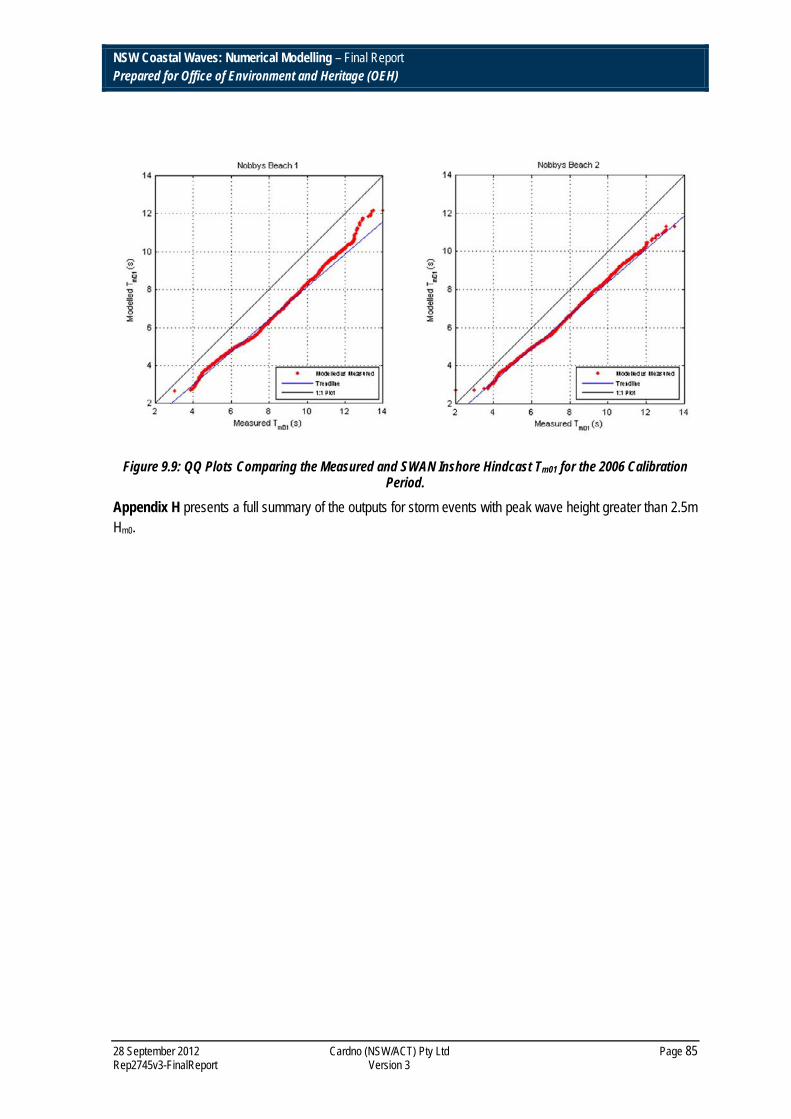
NSW Coastal Waves: Numerical Modelling – Final Report Prepared for Office of Environment and Heritage (OEH)
28 September 2012 Cardno (NSW/ACT) Pty Ltd Page 85 Rep2745v3-FinalReport Version 3
Figure 9.9: QQ Plots Comparing the Measured and SWAN Inshore Hindcast Tm01 for the 2006 Calibration Period.
Appendix H presents a full summary of the outputs for storm events with peak wave height greater than 2.5m Hm0.

NSW Coastal Waves: Numerical Modelling – Final Report Prepared for Office of Environment and Heritage (OEH)
28 September 2012 Cardno (NSW/ACT) Pty Ltd Page 86 Rep2745v3-FinalReport Version 3
10 MODEL VALIDATION – CONTINUOUS SIMULATION WAVE HINDCAST 1998 TO 2009
A continuous hindcast using the coupled WW-III and SWAN models has been undertaken for the period between 1998 and 2009 using the calibrated model system described in Sections 7 to 9. The hindcast for the period from 1998 to 2009 allows for a longer term comparison between modelled and measured wave conditions, and also allows model validation for storm events where significant wave height (Hm0) exceeds 4m to be reliability assessed.
In order to confirm the assessment of the calibration of the WW-III model presented in Section 9.1, over the period of the continuous hindcast, comparisons between the modelled and measured peak wave heights for occasions when the measured significant wave height (Hm0) exceeded 2.5m have been undertaken. Table 10.1 presents a comparison between the average relative error in peak wave height and also the minimum and maximum for all the events over the continuous hindcast period when the significant wave height exceeds 2.5m. Comparing the model outcomes from the calibration period (Table 9.1) and the validation period presented in Table 10.1 indicates that, for significant wave heights exceeding 2.5m, the overall accuracy of the model is higher for the validation period. The general trend of the WW-III model results compared to the Waverider buoy data during the validation period is similar to the calibration period. Generally the model n under predicts the wave height in the order of 5%; with the poorest agreement being observed at Batemans Bay, where the average peak modelled wave height from WW-III is 12.9% lower than the Waverider buoy data.
Table 10.1: Summary of Relative Error (%) between Modelled (WW-III) Peak Wave Height (Hm0>2.5m) and the Measured: 1998 to 2009 where Measured Data is Available
Location No. Of Events
Minimum Maximum Average
Byron Bay 329 -66.1% 79.4% -5.5%
Coffs Harbour 358 -44.5% 49.5% -9.0%
Crowdy Head 358 -48.2% 40.2% -4.2%
Sydney 449 -51.2% 57.3% -7.8%
Port Kembla 406 -65.5% 90.5% -7.9%
Batemans Bay 323 -45.5% 86.7% -12.9%
Eden 439 -48.7% 70.1% -4.3%
When considering the longer term storm wave climate along the NSW coastline, a significant wave height of 2.5m is regularly exceeded (≈ 10% probability of exceedence) and does not represent the extreme wave climate. Generally, studies of the historical NSW wave climate, for example WRL (2011) and Shand et al (2011), define extreme wave conditions along the NSW coast as events where the significant wave height exceeds 4m. Table 10.2 presents a comparison of the average relative errors in peak wave height and also the minimum and maximum for all the events over the continuous hindcast period when the significant wave height exceeds 4m. A significant feature of Table 10.2 is the much larger number of events recorded at Sydney when the wave height exceeds 4m. On average, the model peak wave heights from the WW-III

NSW Coastal Waves: Numerical Modelling – Final Report Prepared for Office of Environment and Heritage (OEH)
28 September 2012 Cardno (NSW/ACT) Pty Ltd Page 87 Rep2745v3-FinalReport Version 3
model system are 5% to 13% lower than measured. Based on Table 10.2, best model agreement with measured data is observed at Crowdy Head and Eden. Table 10.2: Summary of Relative Error (%) between Modelled (WW-III) Peak Wave Height (Hm0>4m) and Measured: 1998 to 2009 where Measured Data is Available
Location No. Of Events
Minimum Maximum Average
Byron Bay 77 -66.1% 37.8% -10.7%
Coffs Harbour 70 -40.0% 45.6% -10.0%
Crowdy Head 74 -43.4% 27.1% -4.6%
Sydney 133 -48.3% 45.6% -11.5%
Port Kembla 90 -41.8% 60.6% -9.2%
Batemans Bay 48 -45.3% 56.5% -13.2%
Eden 86 -38.8% 33.6% -5.0%
Appendix I presents the complete storm table listing and compares the WW-III model and measured peak wave height and associated wave period and direction for all events over the hindcast period when measured significant wave height exceeded 4m.
Table 10.3 presents a summary of the quantitative model validation metrics described in Section 5.8.1 for peak wave height for events with peak greater than 4m significant wave height (Hm0). The validation statistics for the cases when the wave height is greater than 4m significant wave height (Hm0) have shorter periods of continuous analyses compared to the calibration case in Section 10 for the year 2006 when a significant wave height (Hm0) threshold of 2.5m was adopted. As a consequence, the model skill metrics are lower and are more influenced by any slight phase difference between the measured and hindcast peak wave conditions. Overall the validation metrics are reasonable, with a low level of bias for the WW-III modelled wave height and a general, slight under-prediction of the mean wave period by the WW-III model.
Table 10.3: Wave Validation Statistics for the WW-III Model at Deepwater Waverider Buoys (Hm0>4m): 1998 to 2009
Error Statistic
Hm0 Tm01 Tp
Model Skill
Bias (m)
RMS SI (%) R Model Skill
Bias (s)
RMS SI (%) R Model Skill
Bias (s)
RMS SI (%) R
Byron Bay 0.51 -0.26 0.98 20.8% 0.45 0.51 -0.69 1.17 10.7% 0.45 0.62 -1.31 1.92 11.8% 0.62
Coffs Harbour 0.59 -0.35 0.93 18.7% 0.56 0.74 -0.38 0.86 8.8% 0.64 0.68 -1.27 1.79 10.5% 0.68
Crowdy Head 0.67 -0.08 0.72 15.5% 0.54 0.79 -0.15 0.83 9.3% 0.66 0.74 -1.24 1.69 9.5% 0.76
Sydney 0.65 -0.41 0.84 15.5% 0.57 0.80 -0.38 0.79 8.0% 0.72 0.74 -1.19 1.62 9.6% 0.76
Port Kembla 0.54 -0.38 0.81 15.6% 0.47 0.77 -0.49 0.96 9.4% 0.71 0.72 -1.41 1.88 10.5% 0.75
Batemans Bay 0.34 -0.57 0.97 17.2% 0.32 0.67 -0.49 0.93 9.3% 0.59 0.54 -1.60 1.97 9.9% 0.64
Eden 0.64 -0.18 0.76 15.8% 0.52 0.77 -0.22 0.79 9.0% 0.65 0.72 -1.22 1.65 9.7% 0.74
Figure 10.1 presents Quantile-Quantile (Q-Q) plots comparing the measured and modelled wave height distributions for each of the deepwater wave buoy locations over the continuous hindcast period (1998-2009).

NSW Coastal Waves: Numerical Modelling – Final Report Prepared for Office of Environment and Heritage (OEH)
28 September 2012 Cardno (NSW/ACT) Pty Ltd Page 88 Rep2745v3-FinalReport Version 3
At most sites, the wave height distribution of the WW-III model agrees well with the measured up to a significant wave height of 4 to 5m. Above that wave height negative and positive bias trends become more evident.
Figure 10.1: QQ Plots Comparing the Measured and WW-III Hindcast Hm0 for the 1998 - 2009 Hindcast
Figures 10.2 and 10.3 present measured-modelled peak storm wave height plots at each Waverider bouy location and indicate actual storm comparisons, rather than the overall statistical comparisons that are presented in Figure 10.1. The mean trend in Figures 10.2 and 10.3 indicates that the hindcast model may be biased to underestimating peak storm wave heights by between 5% and 13% along the NSW coastline.

NSW Coastal Waves: Numerical Modelling – Final Report Prepared for Office of Environment and Heritage (OEH)
28 September 2012 Cardno (NSW/ACT) Pty Ltd Page 89 Rep2745v3-FinalReport Version 3
Figure 10.2: Scatter Plots Comparing the Measured and WW-III Hindcast Peak Storm Hm0 for the 1998 - 2009 Hindcast – Byron Bay to Sydney

NSW Coastal Waves: Numerical Modelling – Final Report Prepared for Office of Environment and Heritage (OEH)
28 September 2012 Cardno (NSW/ACT) Pty Ltd Page 90 Rep2745v3-FinalReport Version 3
Figure 10.3: Scatter Plots Comparing the Measured and WW-III Hindcast Peak Storm Hm0 for the 1998 - 2009 Hindcast – Port Kembla to Eden
Figure 10.4 presents a set of Q-Q plots comparing the measured and modelled mean wave period (Tm01) distributions for each of the deepwater wave buoy locations over the continuous hindcast period (1998-2009).

NSW Coastal Waves: Numerical Modelling – Final Report Prepared for Office of Environment and Heritage (OEH)
28 September 2012 Cardno (NSW/ACT) Pty Ltd Page 91 Rep2745v3-FinalReport Version 3
Figure 10.4: Q-Q Plots Comparing the Measured and WW-III Hindcast Tm01 for the 1998 - 2009 Hindcast
10.1 Comparison of Modelled and Measured Wave Directions for Peak Storm Wave Heights
Figure 10.5 presents a comparison between modelled (WW-III) and measured peak wave direction histograms for the peak storm wave heights (one value per storm event) when the significant wave height (Hm0) exceeds 4m. The comparisons have been undertaken for the sites when directional wave data is available - Byron Bay, Sydney and Batemans Bay. The results indicate that at Byron Bay the directional distribution of the hindcast storm waves agrees quite well with the measured data, particularly for the northeast to southeast sector. The hindcast wave directions from the WW-III model have fewer events where the peak wave direction is greater than 170O TN. As a consequence, the hindcast data has a greater proportion of peak storm wave conditions in the 160O to 170O TN bin.
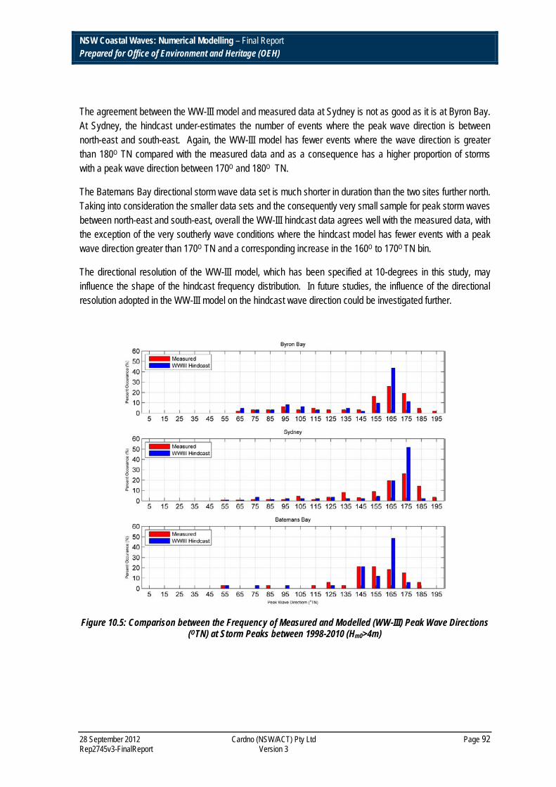
NSW Coastal Waves: Numerical Modelling – Final Report Prepared for Office of Environment and Heritage (OEH)
28 September 2012 Cardno (NSW/ACT) Pty Ltd Page 92 Rep2745v3-FinalReport Version 3
The agreement between the WW-III model and measured data at Sydney is not as good as it is at Byron Bay. At Sydney, the hindcast under-estimates the number of events where the peak wave direction is between north-east and south-east. Again, the WW-III model has fewer events where the wave direction is greater than 180O TN compared with the measured data and as a consequence has a higher proportion of storms with a peak wave direction between 170O and 180O TN.
The Batemans Bay directional storm wave data set is much shorter in duration than the two sites further north. Taking into consideration the smaller data sets and the consequently very small sample for peak storm waves between north-east and south-east, overall the WW-III hindcast data agrees well with the measured data, with the exception of the very southerly wave conditions where the hindcast model has fewer events with a peak wave direction greater than 170O TN and a corresponding increase in the 160O to 170O TN bin.
The directional resolution of the WW-III model, which has been specified at 10-degrees in this study, may influence the shape of the hindcast frequency distribution. In future studies, the influence of the directional resolution adopted in the WW-III model on the hindcast wave direction could be investigated further.
Figure 10.5: Comparison between the Frequency of Measured and Modelled (WW-III) Peak Wave Directions (OTN) at Storm Peaks between 1998-2010 (Hm0>4m)

NSW Coastal Waves: Numerical Modelling – Final Report Prepared for Office of Environment and Heritage (OEH)
28 September 2012 Cardno (NSW/ACT) Pty Ltd Page 93 Rep2745v3-FinalReport Version 3
10.2 Extreme Wave Height Statistics
Table 10.4 presents the Extreme Value Analyses (EVA) of Hm0 for the measured WRB data at the seven deepwater WRBs based on data recorded between 1998 and 2009. These results can be compared with WW-III hindcast model EVA results for the same period of time presented in Table 10.5. It should be noted that since the measured data contains numerous gaps, only the effective number of years has been used in the EVA calculations. See Section 5.2.2 for more details on this calculation. A Weibull distribution with a threshold of Hm0>4m and an independent peak Hm0 threshold of 72 hours has been used in the calculation of all EV statistics. The 95% confidence limits are shown in brackets. Table 10.6 presents the percentage relative error differences between the WW-III model values and the Waverider buoy data values.
For the north coast of NSW, the hindcast model storm wave height distribution is steeper than for the measured data set, which leads to higher 100-years ARI design wave heights. At Byron Bay, the WW-III data set has five additional storms that generated very large waves and for which there were no measurements from the Waverider buoys. WRL (2011) identified that data gaps in the Byron Bay Waverider buoy data set were a limitation in calculating reliable extreme wave statistics. If only the WW-III model results are used for the period when measured data is available (Table I.1), then the 100-years significant wave height from the WW-III model reduces to 7.2m compared to the 8.7m (Table 10.5).
Another key observation at Byron Bay compared to the other sites, is that both the measured and modelled return period calculations have much larger confidence intervals (+/- 1.6m) compared all of the other sites where the 95% confidence interval is typically +/- 0.5 to 1m. The WW-III model also has a large confidence interval at the Coffs Harbour location, which also has more storm events in the WW-III model EV sample compared to the measured data set. This may be caused by the presence of more than one dominant storm type.
At Crowdy Head the agreement between the hindcast WW-III model and the measured peak wave heights distribution is quite good. For the Sydney data set, the hindcast WW-III model has a consistent under-prediction compared to the measured distribution. This is also seen in the measured data set having 133 independent samples of significant wave height exceeding 4m compared to 94 in the WW-III model extreme value sample set. For the south coast from Port Kembla to Eden, the agreement between the modelled and measured EV distributions for peak storm wave height is good.

NSW Coastal Waves: Numerical Modelling – Final Report Prepared for Office of Environment and Heritage (OEH)
28 September 2012 Cardno (NSW/ACT) Pty Ltd Page 94 Rep2745v3-FinalReport Version 3
Table 10.4: Extreme Value Analysis of Hm0 Based on the Measured WRB Data for 1998-2009
ARI (yrs) Byron Bay Coffs
Harbour Crowdy
Head Sydney Port Kembla
Batemans Bay
Eden
1 5.55 (±0.33) 5.61 (±0.27) 5.66 (±0.28) 6.25 (±0.26) 5.55 (±0.26) 5.23 (±0.28) 5.71 (±0.31)
2 5.95 (±0.49) 6.04 (±0.33) 6.08 (±0.35) 6.70 (±0.29) 5.95 (±0.29) 5.67 (±0.36) 6.20 (±0.38)
5 6.43 (±0.73) 6.56 (±0.42) 6.58 (±0.45) 7.24 (±0.33) 6.45 (±0.34) 6.23 (±0.49) 6.82 (±0.49)
10 6.78 (±0.92) 6.92 (±0.51) 6.94 (±0.53) 7.63 (±0.37) 6.82 (±0.37) 6.63 (±0.61) 7.26 (±0.59)
20 7.13 (±1.11) 7.27 (±0.61) 7.28 (±0.61) 8.01 (±0.42) 7.17 (±0.41) 7.03 (±0.73) 7.70 (±0.70)
50 7.56 (±1.37) 7.71 (±0.75) 7.71 (±0.73) 8.48 (±0.49) 7.62 (±0.47) 7.53 (±0.90) 8.26 (±0.86)
100 7.88 (±1.57) 8.03 (±0.86) 8.03 (±0.82) 8.82 (±0.55) 7.96 (±0.52) 7.90 (±1.03) 8.68 (±0.99)
No. Samples 77 70 74 133 90 48 86
Table 10.5: Extreme Value Analysis of Hm0 Based on the WW-III Hindcast Results for 1998-2009
ARI (yrs) Byron Bay Coffs
Harbour Crowdy
Head Sydney Port Kembla
Batemans Bay
Eden
1 5.48 (±0.32) 5.36 (±0.32) 5.58 (±0.26) 5.80 (±0.24) 5.52 (±0.25) 4.90 (±0.24) 5.69 (±0.29)
2 5.98 (±0.48) 5.91 (±0.45) 5.98 (±0.28) 6.19 (±0.26) 5.95 (±0.33) 5.35 (±0.39) 6.18 (±0.37)
5 6.63 (±0.74) 6.63 (±0.69) 6.47 (±0.32) 6.66 (±0.31) 6.47 (±0.45) 5.95 (±0.66) 6.78 (±0.52)
10 7.11 (±0.95) 7.17 (±0.89) 6.81 (±0.35) 6.99 (±0.36) 6.85 (±0.56) 6.40 (±0.90) 7.23 (±0.66)
20 7.60 (±1.19) 7.70 (±1.11) 7.13 (±0.39) 7.30 (±0.42) 7.21 (±0.68) 6.84 (±1.17) 7.66 (±0.81)
50 8.23 (±1.51) 8.40 (±1.43) 7.53 (±0.45) 7.69 (±0.50) 7.67 (±0.84) 7.43 (±1.55) 8.21 (±1.03)
100 8.70 (±1.76) 8.93 (±1.68) 7.82 (±0.50) 7.96 (±0.58) 8.01 (±0.97) 7.88 (±1.85) 8.62 (±1.20)
No. Samples 82 60 82 94 78 47 90
Table 10.6: Percent Relative Error Difference between the WW-IIIMmodelled and Measured Extreme Value Analysis of Hm0 (1998 – 2009)
ARI (yrs) Byron Bay Coffs
Harbour Crowdy
Head Sydney Port Kembla
Batemans Bay
Eden
1 -1.3% -4.5% -1.4% -7.2% -0.5% -6.3% -0.4%
2 0.5% -2.2% -1.6% -7.6% 0.0% -5.6% -0.3%
5 3.1% 1.1% -1.7% -8.0% 0.3% -4.5% -0.6%
10 4.9% 3.6% -1.9% -8.4% 0.4% -3.5% -0.4%
20 6.6% 5.9% -2.1% -8.9% 0.6% -2.7% -0.5%
50 8.9% 8.9% -2.3% -9.3% 0.7% -1.3% -0.6%
100 10.4% 11.2% -2.6% -9.8% 0.6% -0.3% -0.7%

NSW Coastal Waves: Numerical Modelling – Final Report Prepared for Office of Environment and Heritage (OEH)
28 September 2012 Cardno (NSW/ACT) Pty Ltd Page 95 Rep2745v3-FinalReport Version 3
11 WAVE HINDCAST – SELECTED EVENTS FROM 1979 TO 1997
Due to the long data record from the Port Kembla deepwater WRB and, in order to develop a long-term hindcast data set with which to compare to the measured data, the top 30 storm events based on the historical recorded wave data at Port Kembla from 1979 to 1997 were simulated with the wave model system. Simulations were undertaken for a 15-days period surrounding the peak measured wave height conditions at Port Kembla using the adjusted CFSR hindcast wind data. Appendix J presents the summary storm table listing comparing modelled and measured wave conditions for the 30 selected storm events at Port Kembla. The agreement between the WW-III hindcast peak storm wave conditions and measured data is generally very good with an average relative error of -5% for the hindcast peak storm wave height. In particular, the WW-III hindcast model simulated the very intense May 1997 storm event very well and there was only 0.3m difference between hindcast and measured peak storm wave height for that event. The WW-III similarly was in very good agreement with the peak wave height measured at the Sydney (Longreef) deepwater Waverider buoy for that event.
Figure 11.1 presents a scatter plot comparison of the modelled and measured peak storm wave height data set for Port Kembla from 1979 to 2009. The mean trend indicates that the hindcast model may be biased to underestimating peak storm wave heights by 8%.
Table 11.1 shows the EVA of Hm0 for the WW-III hindcast model for the top 30 storm events (from 1979 – 1997) and the continuous hindcast for 1998 to 2009. A total of 31 years has been used for the calculations even though only 30 storms were modelled from the 1979 to 1997 block. Since the top 30 storms were selected on the basis of measured waves at the Port Kembla WRB, due to the variation in the distribution of storm types along the NSW coastline summarised in Section 3 and WRL (2011), these EVA results are only reliable at Sydney and Port Kembla and these locations have been indicated in bold. Table 11.2 shows the EVA of Hm0 for the measured WRB data for all available data. Table 11.3 shows the precent relative error difference between the WW-III modelled values and the measured values. A Weibull distribution with a threshold of Hm0>4m and a independent peak Hm0 threshold of 72 hours has been used in the calculation of all EVA. The 95% confidence limits are shown in brackets. It should be noted that since the measured data contains numerous gaps, only the effective number of years has been used in the EVA calculations for the measured data. See Section 5.2.2 for more details on this calculation.
Compared to the results presented in Section 11, the extension of the hindcast data set to cover the period from 1979 to 2009 has improved the comparison between measured and hindcast peak wave height return values at Sydney significantly. The increase in the modelled and measured wave heights for the longer return period conditions, for example 100-years ARI, compared with the results presented in Section 11, see Tables 11.1 and 11.2, is due to the additional number of large storm events that occurred during the period between 1979 and 1997 being included in the extreme value data sets.

NSW Coastal Waves: Numerical Modelling – Final Report Prepared for Office of Environment and Heritage (OEH)
28 September 2012 Cardno (NSW/ACT) Pty Ltd Page 96 Rep2745v3-FinalReport Version 3
Figure 11.1: Scatter Plots Comparing the Measured and WW-III Hindcast Peak Storm Hm0 for the 1980 - 2010 – Port Kembla
Whilst the agreement between the modelled and measured peak wave height return values at Port Kembla for the 1979 to 2009 period is not as good as for the 1998 to 2009 period, the agreement is still very good. At Sydney the agreement has improved compared to the 1998 to 2009 period, principally due to the very good performance of the hindcast model for the May 1997 storm event. However, the results indicate that at Sydney the WW-III hindcast model still has a general under-prediction of the peak storm wave height compared to the measured data set.

NSW Coastal Waves: Numerical Modelling – Final Report Prepared for Office of Environment and Heritage (OEH)
28 September 2012 Cardno (NSW/ACT) Pty Ltd Page 97 Rep2745v3-FinalReport Version 3
Table 11.1: Extreme Value Analysis of Hm0 Based on the WW-III Hindcast Results for the 30 Top Storms and Continuous 1998-2009 Hindcast
ARI (yrs) Byron Bay Coffs
Harbour Crowdy
Head Sydney Port Kembla
Batemans Bay
Eden
1 5.01 (±0.18) 4.87 (±0.21) 5.31 (±0.21) 5.70 (±0.23) 5.42 (±0.23) 4.81 (±0.22) 5.36 (±0.21)
2 5.53 (±0.27) 5.46 (±0.30) 5.81 (±0.23) 6.31 (±0.29) 6.04 (±0.30) 5.38 (±0.30) 5.85 (±0.24)
5 6.19 (±0.44) 6.23 (±0.43) 6.36 (±0.26) 7.04 (±0.41) 6.80 (±0.43) 6.06 (±0.38) 6.43 (±0.32)
10 6.68 (±0.61) 6.80 (±0.57) 6.74 (±0.28) 7.55 (±0.54) 7.34 (±0.54) 6.54 (±0.46) 6.83 (±0.40)
20 7.16 (±0.78) 7.36 (±0.72) 7.10 (±0.31) 8.04 (±0.68) 7.87 (±0.67) 7.00 (±0.55) 7.20 (±0.50)
50 7.78 (±1.04) 8.10 (±0.94) 7.53 (±0.37) 8.65 (±0.88) 8.54 (±0.84) 7.59 (±0.69) 7.66 (±0.64)
100 8.24 (±1.24) 8.65 (±1.12) 7.85 (±0.42) 9.09 (±1.04) 9.03 (±0.99) 8.01 (±0.82) 7.99 (±0.75)
Table 11.2: Extreme Value Analysis of Hm0 Based on the Measured WRB Data for all the Available Measured Data
ARI (yrs) Byron Bay Coffs
Harbour Crowdy
Head Sydney Port Kembla
Batemans Bay
Eden
1 5.42 (±0.18) 5.48 (±0.20) 5.68 (±0.21) 6.19 (±0.27) 5.65 (±0.22) 5.14 (±0.19) 5.61 (±0.21)
2 5.80 (±0.27) 5.96 (±0.25) 6.14 (±0.26) 6.71 (±0.36) 6.20 (±0.30) 5.58 (±0.28) 6.08 (±0.24)
5 6.27 (±0.39) 6.57 (±0.33) 6.72 (±0.34) 7.37 (±0.51) 6.90 (±0.44) 6.15 (±0.41) 6.67 (±0.31)
10 6.61 (±0.49) 7.02 (±0.40) 7.13 (±0.41) 7.85 (±0.64) 7.43 (±0.56) 6.56 (±0.53) 7.09 (±0.36)
20 6.94 (±0.60) 7.46 (±0.48) 7.52 (±0.49) 8.32 (±0.78) 7.96 (±0.68) 6.97 (±0.65) 7.49 (±0.43)
50 7.37 (±0.75) 8.03 (±0.60) 8.03 (±0.60) 8.93 (±0.98) 8.65 (±0.86) 7.50 (±0.83) 8.01 (±0.52)
100 7.68 (±0.86) 8.46 (±0.70) 8.40 (±0.69) 9.37 (±1.13) 9.17 (±1.00) 7.90 (±0.96) 8.39 (±0.60)
Table 11.3: Percent Relative Error Difference between the WW-III Modelled (30 Top Storms and Continuous 1998-2009 Hindcast) and Measured (All Data) Extreme Value Analyses of Hm0
ARI (yrs) Byron Bay Coffs
Harbour Crowdy
Head Sydney Port Kembla
Batemans Bay
Eden
1 -7.6% -11.1% -6.5% -7.9% -4.1% -6.4% -4.5%
2 -4.7% -8.4% -5.4% -6.0% -2.6% -3.6% -3.8%
5 -1.3% -5.2% -5.4% -4.5% -1.4% -1.5% -3.6%
10 1.1% -3.1% -5.5% -3.8% -1.2% -0.3% -3.7%
20 3.2% -1.3% -5.6% -3.4% -1.1% 0.4% -3.9%
50 5.6% 0.9% -6.2% -3.1% -1.3% 1.2% -4.4%
100 7.3% 2.2% -6.5% -3.0% -1.5% 1.4% -4.8%

NSW Coastal Waves: Numerical Modelling – Final Report Prepared for Office of Environment and Heritage (OEH)
28 September 2012 Cardno (NSW/ACT) Pty Ltd Page 98 Rep2745v3-FinalReport Version 3
12 DISCUSSION
12.1 Performance of Wave Model Systems
This project has produced a comprehensive global and local scale wave model system for the NSW coastline. The objective of this project was to develop this system and verify the performance of the wave model system for storm wave conditions, principally using historical measured data from the NSW deepwater Waverider buoy measurement system which has been in operation at some locations since the early 1970’s. The wave climate along the NSW coastline is typically quite consistent from north to south based purely on wave height distribution. A recent study by the Water Research Laboratory (WRL, 2011) has indicated that although the wave climate is quite consistent along the NSW coastline, the storm climatology between Eden on the south coast and Byron Bay on the far north coast varies significantly.
The validation of the WW-III hindcast model system developed for this project indicates that the model is most reliable and accurate for describing storm wave conditions between Eden and Port Kembla. The particularly good agreement at Eden, which experiences frequent large southerly waves from Southern Tasman Lows that generally pass south of Tasmania, indicates that the wind fields and wave propagation over the southern Tasman Sea are well described in the model system. The model system is able to accurately simulate the larger storm wave events that affect Batemans Bay. However, at this site the more frequent larger wave events, when the significant wave height (Hm0) may peak between 3m and 5m, are generally underestimated by the model system. The accuracy and resolution of the near-coast winds is the most likely source of inaccuracy in the model. Whilst the accuracy and resolution of bathymetric data may also influence the modelled wave conditions inshore, at the location of the deepwater WRB sites along the NSW coast the effects of seabed bathymetry on wave propagation are much less important than the effect that bathymetry has on the propagation of waves from the location of the deepwater WRBs to the coastline.
At Sydney, the WW-III model system consistently simulates smaller peak storm wave heights compared with the measured data, particularly for events with peak wave heights greater than 5m (Hm0). WRL (2011) noted that the Sydney Longreef Waverider buoy data set had a statistically significant outcome of larger storm wave heights compared to other sites along the coast. The reason for this outcome is unknown, but the following factors could contribute to this outcome:-
Seabed topography, which may result in focusing of wave energy near the Sydney Waverider buoy;
The local storm wind climate at Sydney may differ from the Illawarra coastline and wind enhancement may be a more common occurrence off the Sydney coastline; or
A systematic bias in the measurement system which could be a result of the buoy and/or mooring.
An example of variation in peak storm wave height measurements between Port Kembla and Sydney is the June 2006 period presented as Figure 12.1. Within two weeks, two moderately severe storms hit the NSW coast and both events generated a peak significant wave height of over 6m at Sydney, whereas at Port Kembla the peak wave height was approximately 5m for both events. The WW-III model hindcast the storm

NSW Coastal Waves: Numerical Modelling – Final Report Prepared for Office of Environment and Heritage (OEH)
28 September 2012 Cardno (NSW/ACT) Pty Ltd Page 99 Rep2745v3-FinalReport Version 3
wave conditions very well at Port Kembla for both events; however, it was well below the wave heights recorded at the Sydney Waverider buoy.
Figure 12.1: Time Series of Measured and Modelled (WW-III) Deepwater Wave Height at Sydney (Longreef) and Port Kembla - June 2006.
Figure 12.2 presents synoptic charts from the BoM for the period of the 3 June 2006 storm event where the modelled wave height at Sydney is too low, whilst at Port Kembla the WW-III model simulates the storm wave heights well. The figure indicates that the low pressure system is reasonably large and at this scale the synoptic charts do not indicate a significant difference in the atmospheric conditions between Sydney and Port Kembla. It is possible that oceanographic processes may enhance ocean winds in the Sydney region; however, no data was available to investigate this possibility. The reasons for variations in the storm wave heights between Sydney and Port Kembla warrant further investigation in future studies.

NSW Coastal Waves: Numerical Modelling – Final Report Prepared for Office of Environment and Heritage (OEH)
28 September 2012 Cardno (NSW/ACT) Pty Ltd Page 100 Rep2745v3-FinalReport Version 3
Figure 12.2: Bureau of Meteorology Synoptic Charts for the 03/June/2006 Storm Event around Sydney and Port Kembla.
The hindcast model system has been used to investigate the variation in offshore wave conditions along the coastline, primarily as a function of latitude, in order to investigate differences in storm wave conditions from north to south. Figure 12.3 presents the 100-years ARI wave heights at various sites along the NSW coastline at approximately 50km offshore to minimise the potential influence of the coastal model description and bathymetry on wave heights. Results are based on the 1998 to 2009 continuous WW-III model hindcast and are calculated using a Weibull distribution with a wave height threshold of 4m (Hm0).
The outcome is that the model results indicate that the coastline in the Hunter region near Newcastle has the largest offshore wave heights. Between Sydney and Port Kembla, the difference in the 100-years ARI offshore wave height is approximately 0.5m (Hm0). This outcome provides some evidence that there may be some difference in the storm wave climate between these sites and that East Coast Lows often have higher

NSW Coastal Waves: Numerical Modelling – Final Report Prepared for Office of Environment and Heritage (OEH)
28 September 2012 Cardno (NSW/ACT) Pty Ltd Page 101 Rep2745v3-FinalReport Version 3
wave heights in the Sydney region. The region around Batemans Bay has the smallest 100-years ARI wave heights and the sheltering from the southerly swells, together with the reduced influence of East Coast Low storms on extreme waves in this region, are the primary drivers for this outcome. The wave heights offshore of Eden are larger than those near Batemans Bay and at this location waves from Bass Strait, as well as southerly waves from the southern Tasman Sea, cause increased wave heights. The significantly lower wave heights from the OEH WW-III model in the Batemans Bay region are consistent with the outcomes presented in MHL (2010) and Coghlan et al. (2011).
From approximately Port Macquarie northwards, the 100-years ARI offshore wave height is fairly consistent between 9.5m and 10m. The WW-III model output, which has no gaps in the storm wave height sample between 1998 and 2009, appears to provide a more reliable measure of extreme wave height statistics for the far north coast where, to date, gaps in the measured data from Byron Bay and Coffs Harbour have led to higher uncertainty in the design wave conditions at those Waverider buoys compared to other locations along the coast.
Figure 12.3: 100yr ARI Wave Heights (Hm0) along the whole NSW Coastline at Approximately 50km Offshore.

NSW Coastal Waves: Numerical Modelling – Final Report Prepared for Office of Environment and Heritage (OEH)
28 September 2012 Cardno (NSW/ACT) Pty Ltd Page 102 Rep2745v3-FinalReport Version 3
12.2 Comparison between OEH Model System and Public NOAA Global Model System
A comparison between the extreme wave heights calculated based on the WRB measurements, NOAA WW-III model and OEH WW-III model developed in this study has been undertaken. As part of this exercise, the extreme wave height statistics from WRL (2011) have also been compared to those data sets. All of the NOAA WW-III model results presented in the following tables were obtained from the publically available global Wavewatch-III model prepared by NOAA. The model is run on a 1.0o (latitude) by 1.25o (longitude) grid at a 3-hour time interval. The wind forcing for the model system is the GDAS data set described in Section 6.3.
Tables 12.1 to 12.7 present the comparison tables of wave height return values from Byron Bay to Eden up to 100-years ARI. For the analyses from this study (OEH study) presented in Tables 12.1 to 12.7, all of the Cardno outputs adopt a Weibull distribution with a threshold of Hm0>4m and an independent peak Hm0 threshold of 72hours. The 95% confidence limits are shown in brackets. WRL (2011) outputs also adopt a Weibull distribution, but have adopted 90% confidence limits.
The first column in Tables 12.1 to 12.7, which was obtained from WRL (2011), uses all available WRB measurements since the deployment of Waverider buoys at each site (see Section 6.4) and therefore the extreme value statistics cannot be compared with the shorter period of the two WW-III models due to differences in the sample data sets.
The second column of Tables 12.1 to 12.7, which was also obtained from WRL (2011), presents the extreme waves calculated using the NOAA WW-III model. Since the calculation of the statistics from the NOAA WW-III model uses the same time period, and the same output locations from the NOAA WW-III model specified in WRL (2011), these columns can be compared directly. The results indicate that at most locations, the return values from the WRL (2011) and the analyses of the NOAA data undertaken in this project are quite similar. However, the two studies adopt slightly different extreme value analysis methods and the similar results from the WRL (2011) analyses and those obtained in this study suggest that, although slightly different extreme value calculation methods were applied, similar values are obtained.
It should be noted that since the measured data contains numerous gaps, only the effective number of years has been used in the EVA calculations. See Section 5.2.2 for more details on this calculation.
The more refined OEH WW-III model provides better overall agreement with the measured data (30/1/1997 to 1/8/2009) than the NOAA WW-III data at Crowdy Head, Sydney, Port Kembla, Batemans Bay and Eden. However, both the OEH and NOAA WW-III models estimate larger extreme wave heights at Byron Bay and Coffs Harbour compared to the Waverider buoy data. As discussed earlier, missing storm wave data from these two Waverider buoy sites is a likely cause of under estimation of the extreme wave heights at these sites, when based on the Waverider buoy data.
The coarse grid resolution of the NOAA WW-III model is likely to be a significant factor in the poorer performance of this model compared to the OEH WW-III model. The NOAA model has a relatively coarse description of the coastline, which is likely to affect the comparisons at sites like Crowdy Head, which is located near a region where the NSW coastline changes orientation, and also Eden, where the wave

NSW Coastal Waves: Numerical Modelling – Final Report Prepared for Office of Environment and Heritage (OEH)
28 September 2012 Cardno (NSW/ACT) Pty Ltd Page 103 Rep2745v3-FinalReport Version 3
conditions will be influenced by seas and swells that propagate through Bass Strait, as well as from deep Tasman Sea low pressure systems. The lower accuracy, and coarser resolution of the wind forcing in the NOAA WW-III model, is also a likely contributor to the poorer performance of the NOAA model in estimating extreme wave heights at the Waverider buoy sites.
Table 12.1: Comparison of Extreme Value Analyses of Hm0 at Byron Bay
ARI (yrs)
Hm0 (m)
WRL (2011a) OEH Study
Measured NOAA WW-III Measured NOAA WW-III OEH WW-III
All Available 30/1/1997 -
1/8/2009 30/1/1997 -
1/8/2009 30/1/1997 -
1/8/2009 30/1/1997 -
1/8/2009
1 5.2 (± 0.2) - 5.58 (±0.33) 5.37 (±0.29) 5.46 (±0.31)
2 - - 5.98 (±0.49) 5.85 (±0.35) 5.96 (±0.47)
5 - - 6.48 (±0.72) 6.45 (±0.46) 6.61 (±0.72)
10 6.4 (± 0.2) 7.0 (± 0.6) 6.84 (±0.92) 6.89 (±0.55) 7.10 (±0.94)
20 - - 7.18 (±1.11) 7.33 (±0.65) 7.58 (±1.17)
50 7.2 (± 0.3) - 7.62 (±1.38) 7.88 (±0.80) 8.21 (±1.49)
100 7.6 (± 0.3) 8.4 (± 0.8) 7.95 (±1.59) 8.30 (±0.92) 8.69 (±1.75)
Table 12.2: Comparison of Extreme Value Analyses of Hm0 at Coffs Harbour
ARI (yrs)
Hm0 (m)
WRL (2011a) OEH Study
Measured NOAA WW-III Measured NOAA WW-III OEH WW-III
All Available 30/1/1997 -
1/8/2009 30/1/1997 -
1/8/2009 30/1/1997 -
1/8/2009 30/1/1997 -
1/8/2009
1 5.2 (± 0.2) - 5.63 (±0.27) 5.67 (±0.30) 5.34 (±0.33)
2 - - 6.05 (±0.32) 6.18 (±0.38) 5.88 (±0.47)
5 - - 6.56 (±0.41) 6.84 (±0.50) 6.59 (±0.70)
10 6.7 (± 0.3) 7.4 (± 0.6) 6.91 (±0.49) 7.32 (±0.61) 7.12 (±0.90)
20 - - 7.25 (±0.58) 7.78 (±0.73) 7.65 (±1.12)
50 7.7 (± 0.4) - 7.67 (±0.72) 8.39 (±0.92) 8.33 (±1.42)
100 8.1 (± 0.4) 8.9 (± 0.9) 7.97 (±0.83) 8.84 (±1.06) 8.85 (±1.66)

NSW Coastal Waves: Numerical Modelling – Final Report Prepared for Office of Environment and Heritage (OEH)
28 September 2012 Cardno (NSW/ACT) Pty Ltd Page 104 Rep2745v3-FinalReport Version 3
Table 12.3: Comparison of Extreme Value Analyses of Hm0 at Crowdy Head
ARI (yrs)
Hm0 (m)
WRL (2011a) OEH Study
Measured NOAA WW-III Measured NOAA WW-III OEH WW-III
All Available 30/1/1997 -
1/8/2009 30/1/1997 - 1/8/2009
30/1/1997 - 1/8/2009
30/1/1997 - 1/8/2009
1 5.4 (± 0.2) - 5.65 (±0.28) 6.45 (±0.34) 5.58 (±0.26)
2 - - 6.09 (±0.34) 7.03 (±0.44) 5.99 (±0.28)
5 - - 6.63 (±0.42) 7.77 (±0.58) 6.48 (±0.31)
10 7.0 (± 0.4) 8.3 (± 0.8) 7.01 (±0.49) 8.32 (±0.70) 6.83 (±0.34)
20 - - 7.38 (±0.56) 8.86 (±0.84) 7.15 (±0.38)
50 8.0 (± 0.5) - 7.85 (±0.67) 9.56 (±1.02) 7.55 (±0.43)
100 8.5 (± 0.5) 10.0 (± 1.2) 8.19 (±0.75) 10.09 (±1.17) 7.85 (±0.48)
Table 12.4: Comparison of Extreme Value Analyses of Hm0 at Sydney
ARI (yrs)
Hm0 (m)
WRL (2011a) OEH Study
Measured NOAA WW-III Measured NOAA WW-III OEH WW-III
All Available 30/1/1997 -
1/8/2009 30/1/1997 - 1/8/2009
30/1/1997 - 1/8/2009
30/1/1997 - 1/8/2009
1 5.9 (± 0.2) - 6.33 (±0.34) 5.30 (±0.29) 5.89 (±0.34)
2 - - 6.87 (±0.45) 5.79 (±0.45) 6.44 (±0.50)
5 - - 7.55 (±0.63) 6.41 (±0.74) 7.14 (±0.77)
10 7.5 (± 0.4) 7.0 (± 0.6) 8.05 (±0.79) 6.88 (±0.99) 7.65 (±1.00)
20 - - 8.54 (±0.97) 7.33 (±1.26) 8.15 (±1.24)
50 8.6 (± 0.5) - 9.16 (±1.21) 7.92 (±1.63) 8.80 (±1.58)
100 9.0 (± 0.5) 8.6 (± 0.9) 9.63 (±1.41) 8.35 (±1.93) 9.28 (±1.84)

NSW Coastal Waves: Numerical Modelling – Final Report Prepared for Office of Environment and Heritage (OEH)
28 September 2012 Cardno (NSW/ACT) Pty Ltd Page 105 Rep2745v3-FinalReport Version 3
Table 12.5: Comparison of Extreme Value Analyses of Hm0 at Port Kembla
ARI (yrs)
Hm0 (m)
WRL (2011a) OEH Study
Measured NOAA WW-III Measured NOAA WW-III OEH WW-III
All Available 30/1/1997 -
1/8/2009 30/1/1997 - 1/8/2009
30/1/1997 - 1/8/2009
30/1/1997 - 1/8/2009
1 5.4 (± 0.2) - 5.67 (±0.36) 5.30 (±0.28) 5.63 (±0.31)
2 - - 6.18 (±0.52) 5.79 (±0.44) 6.16 (±0.45)
5 - - 6.86 (±0.77) 6.41 (±0.72) 6.84 (±0.68)
10 7.1 (± 0.3) 7.0 (± 0.6) 7.36 (±0.99) 6.88 (±0.96) 7.34 (±0.88)
20 - - 7.87 (±1.22) 7.33 (±1.22) 7.83 (±1.08)
50 8.3 (± 0.4) - 8.53 (±1.54) 7.92 (±1.59) 8.46 (±1.37)
100 8.8 (± 0.5) 8.6 (± 0.9) 9.03 (±1.79) 8.35 (±1.88) 8.94 (±1.59)
Table 12.6: Comparison of Extreme Value Analyses of Hm0 at Batemans Bay
ARI (yrs)
Hm0 (m)
WRL (2011a) OEH Study
Measured NOAA WW-III Measured NOAA WW-III OEH WW-III
All Available 30/1/1997 -
1/8/2009 30/1/1997 - 1/8/2009
30/1/1997 - 1/8/2009
30/1/1997 - 1/8/2009
1 4.9 (± 0.2) - 5.18 (±0.29) 5.97 (±0.26) 4.97 (±0.28)
2 - - 5.64 (±0.38) 6.42 (±0.28) 5.49 (±0.41)
5 - - 6.20 (±0.51) 6.98 (±0.32) 6.19 (±0.64)
10 6.3 (± 0.4) 7.5 (± 0.6) 6.61 (±0.62) 7.38 (±0.36) 6.73 (±0.85)
20 - - 7.01 (±0.74) 7.77 (±0.41) 7.27 (±1.09)
50 7.3 (± 0.5) - 7.53 (±0.91) 8.27 (±0.49) 7.98 (±1.44)
100 7.7 (± 0.5) 8.8 (± 0.9) 7.91 (±1.05) 8.63 (±0.56) 8.53 (±1.72)

NSW Coastal Waves: Numerical Modelling – Final Report Prepared for Office of Environment and Heritage (OEH)
28 September 2012 Cardno (NSW/ACT) Pty Ltd Page 106 Rep2745v3-FinalReport Version 3
Table 12.7: Comparison of Extreme Value Analyses of Hm0 at Eden
ARI (yrs)
Hm0 (m)
WRL (2011a) OEH Study
Measured NOAA WW-III Measured NOAA WW-III OEH WW-III
All Available (17/7/1987 –
1/8/2009)
30/1/1997 - 1/8/2009
30/1/1997 - 1/8/2009 30/1/1997 -
1/8/2009 30/1/1997 -
1/8/2009
1 5.4 (± 0.2) - 5.71 (±0.31) 4.67 (±0.26) 5.67 (±0.30)
2 - - 6.20 (±0.37) 5.05 (±0.31) 6.16 (±0.38)
5 - - 6.81 (±0.47) 5.50 (±0.35) 6.77 (±0.53)
10 7.0 (± 0.3) 5.9 (± 0.4) 7.25 (±0.57) 5.82 (±0.39) 7.21 (±0.67)
20 - - 7.68 (±0.68) 6.12 (±0.43) 7.64 (±0.82)
50 8.1 (± 0.4) - 8.24 (±0.84) 6.50 (±0.50) 8.19 (±1.03)
100 8.5 (± 0.5) 6.8 (± 0.5) 8.65 (±0.96) 6.78 (±0.57) 8.60 (±1.20)
12.3 Ambient Wave Climate Model Capability
A preliminary analysis of the performance of the wave model system for describing the overall wave climate along the NSW coastline, including ambient sea state conditions, has been undertaken for three locations along the NSW coast – Byron Bay, Sydney and Eden. The results indicate that the RMS error is similar at these three sites. The bias results indicate that for Sydney wave heights are generally lower for the WW-III model. At Eden and Byron Bay, the bias is generally very small. The validation metrics presented in Figure 12.4 are consistent with the WW-III validation for North America presented in Chawla et al (2009). This outcome indicates that the model system developed for this project has potential to be further developed to apply to hindcasting of ambient sea state conditions.
Figure 12.4: Validation Metrics (Bias, RMS Error and Scatter Index) Presented Top to Bottom Based on the
Whole 2006 Hindcast Period for Byron Bay (left), Sydney (centre) and Eden (right)

NSW Coastal Waves: Numerical Modelling – Final Report Prepared for Office of Environment and Heritage (OEH)
28 September 2012 Cardno (NSW/ACT) Pty Ltd Page 107 Rep2745v3-FinalReport Version 3
12.4 SWAN Model System
The SWAN model has been applied in two components of the model system developed for this project. Firstly, a SWAN model has been developed along the whole NSW coastline, and extending to approximately 150m to 200m depth offshore. This model provides a single regional scale model (2.5km grid resolution) that can transfer the WW-III model outputs to the NSW coastline. The model is designed so that high resolution local scale SWAN models with grid resolutions of 100m or less can be coupled with the model to enable accurate hindcasting of wave conditions up to the shorelines and inside entrances along the coast. The whole of NSW SWAN transition model has been developed as a regular, structured grid. This study has identified differences in the wind growth physics between SWAN and WW-III that can lead to significant differences in the wave frequency spectrum, even at the deepwater Waverider buoy locations. This limitation is most significant during southerly or offshore wind conditions along the NSW coastline where there is sufficient fetch length within the SWAN model to simulate sea wave conditions and during these conditions, the SWAN model has poorer agreement at the deepwater WRBs compared to WW-III for wave period.
The near shore SWAN model of Newcastle developed for this study has been validated with measured wave data from near the entrance to Newcastle Harbour. The Newcastle model has been developed as an irregular grid with variable grid resolution. That model has achieved very good agreement for measured storm wave heights compared to the measured data.
12.5 Areas for Future Development of the Model System
The WW-III and SWAN wave model systems developed for this project have achieved a high level of validation for storm wave conditions along the NSW coastline, particularly for the region from Eden to Port Kembla. The study has indicated that although the WW-III and SWAN model systems are advanced model systems that can simulate wave processes well, there are some areas of improvement for the wave model systems. Both WW-III and SWAN displayed a negative bias for wave period along the NSW coastline and this was particularly significant with the SWAN wave model. The results for this study would indicate that overall, the wave growth physics in the WW-III model system are superior to those in the SWAN model system. The SWAN model tends to overestimate the proportion of wave energy in the high frequency ends of the spectra. Ideally, the deepwater and near shore wave model systems with a coupled model should have consistent wind growth physics and the Tolman and Chalikov (1996) model adopted in the WW-III model appears to be more accurate than the wind growth models available in SWAN. The most desirable model system would have integrated physics for deepwater and shallow water so that a single model system could be applied. In the absence of an integrated deepwater and shallow water wave model, future development of the OEH wave model system may consider directly coupling near shore SWAN wave models to the OEH WW-III model outputs with the coupling boundary between the model located in 50m to 100m water depth.
The adjusted CFSR wind field data set applied in this study has generated realistic wave conditions along the NSW coastline. High accuracy of the wave model system compared to the measured Waverider buoy data at Eden suggests that the CFSR winds are most accurate for describing large scale ocean wind forcing conditions away from a large landmass. This is consistent with similar conclusions from large scale verification of the CFSR data set (Cardone et al, 2011). The true accuracy of the CFSR winds for the near

NSW Coastal Waves: Numerical Modelling – Final Report Prepared for Office of Environment and Heritage (OEH)
28 September 2012 Cardno (NSW/ACT) Pty Ltd Page 108 Rep2745v3-FinalReport Version 3
coast region of NSW, which does affect wave conditions for the coastline north of Eden up to Byron Bay, is unknown. Long duration (minimum of 1-year) ‘over-water’ wind measurements at one or more sites off the NSW coastline would provide a valuable data set to assess the accuracy of global scale wind field data sets and to also investigate if there are variations in the over-water wind conditions along the coast that may be driving outcomes such as the significantly higher storm wave height at Sydney compared to Port Kembla. Over-water wind measurements from a met-buoy deployed in a study area is the most reliable method to validate ocean and coastal wind conditions which may influence wave climate along the NSW coast.
Some storm systems, for example, very intense East Coast Lows such as the June 2007 or May 1974 storms, may have very steep spatial and short temporal scales in wind conditions. The resolution of global scale wind data sets, which at best are 25km, may be too coarse to describe the winds which cause variable peak wave conditions along short extents of coastline, for example, Port Kembla to Sydney. The WW-III and SWAN model system developed in this project could be forced with alternative wind field data sets from down-scaled high-resolution atmospheric models. These high resolution winds could be blended into a larger scale global data set. If high-resolution coastal hindcast winds are available for NSW, it is recommended that OEH consider modelling a period of time, for example, year 2006 to investigate whether or not down-scaled wind modelling can improve the accuracy of the wave model system.
The model system developed in this study is highly computationally efficient and could be utilised in a forecast based model system, provided that accurate forecast wind data, for example the BoM’s AUSWIND/AUSWAVE forecast model system, could be applied to force the model in the Australian region.
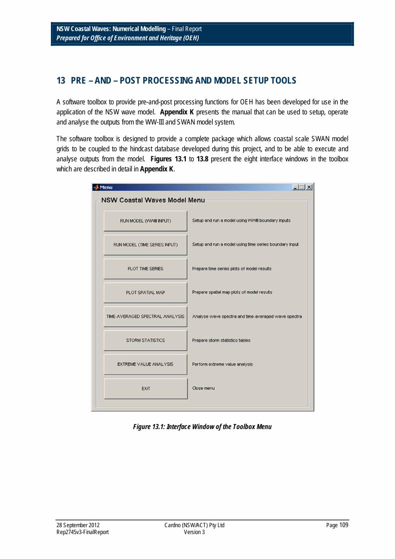
NSW Coastal Waves: Numerical Modelling – Final Report Prepared for Office of Environment and Heritage (OEH)
28 September 2012 Cardno (NSW/ACT) Pty Ltd Page 109 Rep2745v3-FinalReport Version 3
13 PRE – AND – POST PROCESSING AND MODEL SETUP TOOLS
A software toolbox to provide pre-and-post processing functions for OEH has been developed for use in the application of the NSW wave model. Appendix K presents the manual that can be used to setup, operate and analyse the outputs from the WW-III and SWAN model system.
The software toolbox is designed to provide a complete package which allows coastal scale SWAN model grids to be coupled to the hindcast database developed during this project, and to be able to execute and analyse outputs from the model. Figures 13.1 to 13.8 present the eight interface windows in the toolbox which are described in detail in Appendix K.
Figure 13.1: Interface Window of the Toolbox Menu

NSW Coastal Waves: Numerical Modelling – Final Report Prepared for Office of Environment and Heritage (OEH)
28 September 2012 Cardno (NSW/ACT) Pty Ltd Page 110 Rep2745v3-FinalReport Version 3
Figure 13.2: Interface Window of the Toolbox used for Setting Up and Running a Model using the WW-III Boundary Inputs.

NSW Coastal Waves: Numerical Modelling – Final Report Prepared for Office of Environment and Heritage (OEH)
28 September 2012 Cardno (NSW/ACT) Pty Ltd Page 111 Rep2745v3-FinalReport Version 3
Figure 13.3: Interface Window of the Toolbox used for Setting Up and Running a Model using a Time-Series File for Boundary Conditions

NSW Coastal Waves: Numerical Modelling – Final Report Prepared for Office of Environment and Heritage (OEH)
28 September 2012 Cardno (NSW/ACT) Pty Ltd Page 112 Rep2745v3-FinalReport Version 3
Figure 13.4: Interface Window of the Toolbox used for Plotting Time-Series Results

NSW Coastal Waves: Numerical Modelling – Final Report Prepared for Office of Environment and Heritage (OEH)
28 September 2012 Cardno (NSW/ACT) Pty Ltd Page 113 Rep2745v3-FinalReport Version 3
Figure 13.5: Interface Window of the Toolbox used for Plotting of Spatial Map Results

NSW Coastal Waves: Numerical Modelling – Final Report Prepared for Office of Environment and Heritage (OEH)
28 September 2012 Cardno (NSW/ACT) Pty Ltd Page 114 Rep2745v3-FinalReport Version 3
Figure 13.6: Interface Window of the Toolbox used for Extracting and Plotting Time-Averaged Wave Spectra

NSW Coastal Waves: Numerical Modelling – Final Report Prepared for Office of Environment and Heritage (OEH)
28 September 2012 Cardno (NSW/ACT) Pty Ltd Page 115 Rep2745v3-FinalReport Version 3
Figure 13.7: Interface Window of the Toolbox used for Creating Storm Summary Tables and Statistics

NSW Coastal Waves: Numerical Modelling – Final Report Prepared for Office of Environment and Heritage (OEH)
28 September 2012 Cardno (NSW/ACT) Pty Ltd Page 116 Rep2745v3-FinalReport Version 3
Figure 13.8: Interface Window of the Toolbox used for Performing Extreme Value Analyses
NSW Coastal Waves: Numerical Modelling – Final Report Prepared for Office of Environment and Heritage (OEH)
28 September 2012 Cardno (NSW/ACT) Pty Ltd Page 117 Rep2745v3-FinalReport Version 3
14 CONCLUSIONS
This report has described the development of the wave model system for the NSW coastline as part of the contract awarded to Cardno (Contract: DECCW-57-2011). The project has required the development of a wave model system that includes a global scale WW-III model together with a whole of NSW coastal SWAN near shore wave model.
As part of this project an extensive array of wave, wind and bathymetric data has been compiled. During the development of the model system, the most suitable input data sets were identified. The wind data applied to the model (CFSR) has been calibrated with measured ‘over-water’ winds and QuickSCAT scatterometry wind data. The calibration process identified a requirement to adjust upwards wind speeds within 100km of land along the NSW coastline.
The wave model system has been developed with carefully attention to the physics of the WW-III and SWAN models to ensure a robust model is developed and to minimise any Relative Error between results from the two model systems. A comprehensive assessment of the sensitivity of model systems, both near shore and offshore, has been undertaken for key parameter settings and coefficients adopted in the two wave model systems.
The wave model system has been calibrated using measured Waverider buoy data for 2006. The WW-III model has been identified as the model system which best simulates wave conditions at the deepwater Waverider buoys. The SWAN wave model shows good agreement with measured wave heights, but has a consistent negative bias for mean wave period. The overall model system has demonstrated generally good calibration for peak storm wave heights, particularly for the south coast of NSW. The source of relative error between modelled and Waverider buoy wave heights at the Sydney Waverider buoy is unknown, especially considering that the model calibration at Port Kembla approximately 150km south is very good. The SWAN model has been calibrated for near shore wave conditions with data from the entrance to Newcastle Harbour. The inshore SWAN model has good agreement with measured (WRB) peak storm wave heights at that location.
A continuous hindcast from 1998 to 2009 along the whole NSW coastline with outputs at 1-hourly time steps has been undertaken. Between 1979 and 1997, this study has also simulated the top 30 storms (based on wave height) from the Port Kembla Waverider buoy data set as this is the longest continuous Waverider bouy data that was available in this study. Analyses of outputs in the form of extreme wave statistics from the WW-III model have been compared to statistics from WRL (2011), results from the NOAA public global scale WW-III model and of measured Waverider buoy data. The model system appears to estimate wave height return values well for the south and mid-NSW coast with the exception of Sydney. As mentioned previously, the source of relative error between modelled and measured storm wave heights at Sydney is unknown. The wave model system appears to provide a more reliable estimate of wave height return values for the north coast compared to the Waverider buoy data sets which are affected by gaps in the data during key storm events (WRL, 2011).

NSW Coastal Waves: Numerical Modelling – Final Report Prepared for Office of Environment and Heritage (OEH)
28 September 2012 Cardno (NSW/ACT) Pty Ltd Page 118 Rep2745v3-FinalReport Version 3
This project has developed a comprehensive model tool with a Graphical User Interface (GUI) to run the NSW scale SWAN model and any user specified near shore SWAN model. The tool provides a comprehensive array of functions for post-processing and data analysis including Extreme Value Analysis using the Maximum Likelihood Method.

NSW Coastal Waves: Numerical Modelling – Final Report Prepared for Office of Environment and Heritage (OEH)
28 September 2012 Cardno (NSW/ACT) Pty Ltd Page 119 Rep2745v3-FinalReport Version 3
15 REFERENCES
Atlas, R., R. N. Hoffman, S. C. Bloom, J. C. Jusem, and J. Ardizzone, (1996). A multiyear global surface wind velocity data set using SSM/I wind observations. Bull. Amer. Meteor. Soc., 77, 869–882.
Atlas R., R., and R. N. Hoffman, (1999). The Use of Satellite Surface Wind Data to Improve Weather Analysis and Forecasting. Satellites, Oceanography, and Society.
Amante, C. and Eakins B. W., (2009). ETOPO1 1 Arc-Minute Global Relief Model: Procedures, Data Sources and Analysis. NOAA Technical Memorandum NESDIS NGDC-24, 19 pp, March 2009.
Bunney C (2011). A High Resolution SWAN Model Assessment: North Norfolk to Humber. Forecasting Research Technical Report 557. Prepared by UK Met Office.
Battjes, J.A. and J.P.F.M. Janssen, (1978). Energy Loss and Set-up Due to Breaking of Random Waves, Proc. 16 th Int. Conf. Coastal Engineering, ASCE, pp 569-587.
Booij, N. and L. H. Holthuijsen, (1987). Propagation of Ocean Waves in Discrete Spectral Wave Models. J. Comput. Physics. 68, 307-326.
Booij, N., R. C. Ris and L. H. Holthuijsen, (1999). A Third-Generation Wave Model for Coastal Regions, Part I, Model Description and Validation. J. Geophys. Res., 104, 7649-7666.
Bouws, E. and G. J. Komen, (1983). On the Balance between Growth and Dissipation in an Extreme Depth-Limited Wind-Sea in the Southern North Sea. J. Phys. Oceanogr., 13, pp. 1653-1658.
Caires, S., J. Groenweg and A. Sterl. (2006). “Changes in the North Sea Extreme Waves” Proceedings of 9th international workshop on wave hindcasting and forecasting, September 2006, Victoria, BC, Canada. Cardone V., Cox A. T., Orelup E. A., Morrone M. and Swail V.R., (2011). “Specification of Unbiased and Homogeneous Marine Wind Analyses – Progress and Critical Issues”. Proceedings of the Third International Workshop on Advances in the Use of Historical Marine Climate Data. MARCDAT-III, Frascati, Italy, 2-6 May Chawla, A., Tolman, H.L., Hanson, J.L., Devaliere, E.M., Gerald, V.M. (2009). “Validation of a Multi-Grid WAVEWATCH III Modeling System” 11th Waves Forecasting and Hindcasting Workshop, 2009, Halifax, Nova Scotia, Canada. Chawla A., Sprindler D and Tolman H., (2011). “Wavewatch-III Hindcasts with Re-analysis winds. Initial report on model setup”. National Centers for Environmental Prediction, MMAB Contribution No. 291. Draft, April 2011. Coghlan et al. (2011). “High Resolution Wave Modelling (HI-WAM) for Batemans Bay Detailed Wave Study.” Proceedings of Australasian Coasts and Ports Conference, Perth. September 2012. Eldeberky, Y., (1996). Nonlinear transformation of wave spectra in the nearshore zone, Ph.D. thesis, Delft University of Technology, Department of Civil Engineering, The Netherlands

NSW Coastal Waves: Numerical Modelling – Final Report Prepared for Office of Environment and Heritage (OEH)
28 September 2012 Cardno (NSW/ACT) Pty Ltd Page 120 Rep2745v3-FinalReport Version 3
Geoscience Australia (2009). GEODATA 9 Second Digital Elevation Model (DEM-9S) Version 3. Prepared by Geoscience Australia. Available at: http://www.ga.gov.au/meta/ANZCW0703011541.html
Goda Y. (2000). "Random Seas and the Design of Maritime Structures". Advanced Series on Ocean Engineering – Volume 15. World Scientific, Singapore 2000.
Goda Y. (1988). "On the methodology of selecting design wave height." Proceedings 21st International Conference Coastal Engineering. pp899-913.
Goda Y. (1992). "Uncertainty of Design Parameters From Viewpoint of Extreme Statistics". Journal of Offshore Mechanics and Arctic Engineering. Vol 114, pp76-82, May 1992.
Gringorten I. I (1963) "A plotting rule for extreme probability paper" Journal of Geophysical Research. Vol 68 (3) pp 813-814.
Hasselmann, K., (1974). On the spectral dissipation of ocean waves due to whitecapping, Bound.-layer Meteor., 6, 1-2, 107-127
Hasselmann, K., T. P. Barnett, E. Bouws, H. Carlson, D. E. Cartwright, K. Enke, J. A. Ewing, H. Gienapp, D. E. Hasselmann, P. Kruseman, A. Meerburg, P. Mueller, D. J. Olbers, K. Richter, W. Sell and H. Walden, (1973). Measurements of wind-wave growth and swell decay during the Joint North SeaWave Project (JONSWAP). Ergaenzungsheft zur Deutschen Hydrographischen Zeitschrift, Reihe A(8), 12, 95 pp.
Hopkins L.C. and Holland G. J., (1997). Australian Heavy-Rain Days and Associated East Coast Cyclones: 1958 to 1992. Monthly Weather Review. Vol. 115, pp 3024-3026.
Janssen, P.A.E.M., (1989). Wave induced stress and the drag of air flow over sea waves, J. Phys. Oceanogr., 19, 745-754.
Janssen, P.A.E.M., (1991). Quasi-linear theory of wind-wave generation applied to wave forecasting, J. Phys. Oceanogr., 21, 1631-1642
Kinsman, D (2002). Wind Waves, Their Generation and Propagation on the Ocean Surface. Dover Publications.
Komen, G.J., Cavaleri, L., Donelan, M., Hasselmann, K., Hasselmann, S. and P.A.E.M. Janssen, (1994). Dynamics and Modelling of Ocean Waves, Cambridge University Press, 532 p.
Lord D. and Kulmer M. (2000). “The 1974 Storms Revisited: 25-Years Experience in Ocean Wave Measurement along the South-East Australian Coast”. Proceedings of Coastal Engineering 2000. Sydney, 2000.
Mathiesen M, Goda Y, Hawkes P J, Mansard E, Martin M J, Peltier E, Thompson E F and van Vledder G (1994) “Recommended Practice for Extreme Wave Analysis”. Journal of Hydraulic Research. Vol. 32 1994 No 6.
Manly Hydraulics Laboratory (2010). Batemans Bay Wave Climate Study, MHL Report 2003 (Draft).
NSW Coastal Waves: Numerical Modelling – Final Report Prepared for Office of Environment and Heritage (OEH)
28 September 2012 Cardno (NSW/ACT) Pty Ltd Page 121 Rep2745v3-FinalReport Version 3
Naess A and Hungnes B. (2002). "Estimating Confidence Intervals of Long Return Period Design Values by Bootstrapping". Journal of Offshore and Arctic Engineering. American Society of Mechanical Engineers.
Naess A and Hungnes B. (2002). "Estimating Confidence Intervals of Long Return Period Design Values by Bootstrapping". Journal of Offshore and Arctic Engineering. American Society of Mechanical Engineers.
PWD (1985). “Elevated ocean levels – Storms affecting the NSW coast 1880 to 1980.” Report No. 85041. Report prepared by Blain, Bremner and Williams Pty Ltd.
Rogers, W. E., and Campbell, T. J. “Implementation of Curvilinear Coordinate System in the WAVEWATCH III Model.” Naval Research Laboratory, NRL/MR/7320—09-9193, United States Navy, September 2009.
Shand T D, Wasko C D, Goodwin I D, Carley J T, You Z J, Kulmar M and Cox R J. (2011). “Long Term Trends in NSW Coastal Wave Climate and Derivation of Extreme Design Storms”. Proceedings of Coasts and Ports 2011. September 2011. Published by Engineers Australia.
Taylor D. R. (2006)’ Nonlinear Estimation of Extreme Value Model Parameters in Coastal and Ocean Engineering’. Graduate paper from Queen’s University, Canada. Course CHEE-824: Non-linear regression. April 2006.
Padill-Hernandez R., Perrie W., Toulany B., and Smith P. C., (2007). Inter-comparison of Third Generation Wave Models. Weather and Forecasting. Vol 22 No 6. Pp 1229-1242.
Taylor D. R. (2006). ‘Nonlinear Estimation of Extreme Value Model Parameters in Coastal and Ocean Engineering’. Graduate paper from Queen’s University, Canada. Course CHEE-824: Non-linear regression. April 2006.
Tolman, H. L., (1992). Effects of Numerics on the Physics in a third-generation wind-wave model. Journal of Physical Oceanography., 22, 1095-1111.
Tolman, .H. L., (1995). On the selection of propagation schemes for a spectral wind wave model. Office Note 411, NSW/NCEP, 30 pp + figures.
Tolman, H. L., (1997). User manual and system documentation of WAVEWATCH-III version 1.15. NOAA/NWS/NCEP/OMB. Technical Note 151, 97 pp.
Tolman, H. L., (1999). User manual and system documentation of WAVEWATCH III version 1.18. Tech Note 166, NOAA/NWS/NCEP/OMB, 110 pp.
Tolman, H. L., (2002a). Alleviating the garden sprinkler effect in wind wave models. Ocean Mod., 4, 269-289.
Tolman, H. L., (2002b). Limiters in third-generation wind wave models. The Global Atmosphere and Ocean System, 8, 67-83.
Tolman, H. L., (2002c). User manual and system documentation of WAVE-WATCH III version 2.22. Tech Note 222, NOAA/NWS/NCEP/MMAB, 133 pp.

NSW Coastal Waves: Numerical Modelling – Final Report Prepared for Office of Environment and Heritage (OEH)
28 September 2012 Cardno (NSW/ACT) Pty Ltd Page 122 Rep2745v3-FinalReport Version 3
Tolman, H. L., (2009). User manual and system documentation of WAVEWATCH III version 3.14. Tech Note, NOAA/NWS/NCEP/MMAB, 220 pp.
U.S. Army Corps of Engineers. (2002). Coastal Engineering Manual. Engineer Manual 1110-2-1100, U.S. Army Corps of Engineers, Washington, D.C. (in 6 volumes).
van Vledder G, Goda Y, Hawkes P, Mansard E, Martin M, Mathiesen M, Thompson E F and Peltier E (1993). "Case studies of Extreme Wave Analysis: a Comparative Analysis." Ocean Wave Measurement and Analysis – Proceedings of the Second International Symposium. New Orleans, Louisiana.
Water Research Laboratory (2011). “NSW Coastal Inundation Hazard Study: Coastal Storms and Extreme Waves. Technical Report 2010/16. January 2011.
Willmott, C.J., Ackleson, S.G., Davis, R.E,, Feddema, J.J., Klink, K.M., Legates, D.R., O’Donnell, J. and Rowe, C.M. (1985). ‘Statistics for the Evaluation and Comparison of Models’, Journal of Geophysical Research, Vol.90, No. C5, pages 8995-9905, September 20, 1985.
Wyllie S.J., and Kulmer, M. A. (1995), Coastal Wave Monitoring. Australian Marine Data Collection and Management Guidelines Workshop. Environmental Resources Information Network, Hobart, December 1995.

28 September 2012 Cardno (NSW/ACT) Pty Ltd Page A1 S:\Projects\J1001_CardnoHandoverProjects\008_ReportingDocsandFigures\LJ2949-NSWWaveModelling\Rep2745v3-FinalReport\Rep2745v3-FinalReport.docx Version 1
Appendix B OEH Compiled Bathymetric Metadata (including LiDAR)
Appendix A OEH Compiled Bathymetry Metadata (including LiDAR)

28 September 2012 Cardno (NSW/ACT) Pty Ltd Page A1 S:\Projects\J1001_CardnoHandoverProjects\008_ReportingDocsandFigures\LJ2949-NSWWaveModelling\Rep2745v3-FinalReport\Rep2745v3-FinalReport.docx Version 1
Appendix B WWIII Hindcast Validation Time Series – Deepwater WRBs (2006)

28 September 2012 Cardno (NSW/ACT) Pty Ltd Page A1 S:\Projects\J1001_CardnoHandoverProjects\008_ReportingDocsandFigures\LJ2949-NSWWaveModelling\Rep2745v3-FinalReport\Rep2745v3-FinalReport.docx Version 1
Appendix C Storm Event Comparisons – WWIII 2006 Hindcast – Deepwater WRBs
(Hm0>2.5m)

28 September 2012 Cardno (NSW/ACT) Pty Ltd Page A1 S:\Projects\J1001_CardnoHandoverProjects\008_ReportingDocsandFigures\LJ2949-NSWWaveModelling\Rep2745v3-FinalReport\Rep2745v3-FinalReport.docx Version 1
Appendix D WWIII Hindcast Validation Scatter Plots – Deepwater WRBs (2006)

28 September 2012 Cardno (NSW/ACT) Pty Ltd Page A2 S:\Projects\J1001_CardnoHandoverProjects\008_ReportingDocsandFigures\LJ2949-NSWWaveModelling\Rep2745v3-FinalReport\Rep2745v3-FinalReport.docx Version 1
Appendix E SWAN (Transition) Hindcast Validation Time Series – Deepwater
WRBs (2006)

28 September 2012 Cardno (NSW/ACT) Pty Ltd Page A3 S:\Projects\J1001_CardnoHandoverProjects\008_ReportingDocsandFigures\LJ2949-NSWWaveModelling\Rep2745v3-FinalReport\Rep2745v3-FinalReport.docx Version 1
Appendix F Storm Event Comparisons – SWAN (Transition) 2006 Hindcast –
Deepwater WRBs (Hm0>2.5m)

28 September 2012 Cardno (NSW/ACT) Pty Ltd Page A4 S:\Projects\J1001_CardnoHandoverProjects\008_ReportingDocsandFigures\LJ2949-NSWWaveModelling\Rep2745v3-FinalReport\Rep2745v3-FinalReport.docx Version 1
Appendix G SWAN (Inshore) Hindcast Validation Time Series – Nobby’s Beach
Inshore WRBs (2006)

28 September 2012 Cardno (NSW/ACT) Pty Ltd Page A5 S:\Projects\J1001_CardnoHandoverProjects\008_ReportingDocsandFigures\LJ2949-NSWWaveModelling\Rep2745v3-FinalReport\Rep2745v3-FinalReport.docx Version 1
Appendix H Storm Event Comparisons – SWAN (Inshore) 2006 Hindcast –
Nobby’s Beach WRBs (Hm0>2.5m)

28 September 2012 Cardno (NSW/ACT) Pty Ltd Page A6 S:\Projects\J1001_CardnoHandoverProjects\008_ReportingDocsandFigures\LJ2949-NSWWaveModelling\Rep2745v3-FinalReport\Rep2745v3-FinalReport.docx Version 1
Appendix I Storm Event Comparisons – WWIII 1998-2009 Hindcast – Deepwater
WRBs (Hm0>4.0m)

28 September 2012 Cardno (NSW/ACT) Pty Ltd Page A7 S:\Projects\J1001_CardnoHandoverProjects\008_ReportingDocsandFigures\LJ2949-NSWWaveModelling\Rep2745v3-FinalReport\Rep2745v3-FinalReport.docx Version 1
Appendix J Storm Event Comparisons – WWIII Top 30 Storms Hindcast – Port
Kembla Deepwater WRB

28 September 2012 Cardno (NSW/ACT) Pty Ltd Page A8 S:\Projects\J1001_CardnoHandoverProjects\008_ReportingDocsandFigures\LJ2949-NSWWaveModelling\Rep2745v3-FinalReport\Rep2745v3-FinalReport.docx Version 1
Appendix K Machine Configuration and User Manual