Numerical Modelling in Fortran: day 2Paul Tackley, 2019

Goals for today• Review main points in online materials you

read for homework – http://www.cs.mtu.edu/%7eshene/COURSES/cs201/NOTES/intro.html

• More details about loops• Finite difference approximation• Introduce and practice

– subroutines & functions– arrays

Miscellaneous things• Continuing lines:

– f95 use �&� at the end of the line– f77: put any character in column 6 on next line

• Formats of constants:– Use �.� to distinguish real from integer (avoid 2/3=0 !)– 1.234x10-13 is written as 1.234e-13

• logical variables have 2 values: .true. or .false.• Variable naming rules:

– start with letter– mix numbers, letters and _– no spaces

Character/string definitions

• character :: a (single character)• character(len=10) :: a (string of length 10)• character :: a*10, b*5 • character*15:: a,b (fortran77 style)• character(len=*),parameter :: Name=�Paul�

– automatic length, otherwise strings will be truncated or padded with spaces to fit declared length

Initialising variables

• Always initialise variables! Don�t assume they will automatically be set to 0!

• Either– when defined, e.g., real:: a=5.– in the program, e.g., a=5.0– read from keyboard or file

Arithmetic operators• e.g., what does a+b*c**3 mean?

– ((a+b)*c)**3? a+(b*c)**3? etc.– No! correct is: a+(b*(c**3))– priority is **, (* or /) then (+ or -)

• Also LOGICAL operators, in this priority:– .not., .and., .or., (.eqv. or .neqv.)

• Be careful mixing variable types (e.g. integer & real) in the same expression!

Some intrinsic mathematical functions

• abs (absolute value, real or integer)• sqrt (square root)• sin, cos, tan, asin, acos, atan, atan2:

assume angles are in radians• exp and log : log is natural log, use log10

for base 10. • also cosh, sinh, tanh• for full list see a manual

Some conversion functions• Int(a): round to smaller # (4.7->4; -4.6->-4)• Nint(a): nearest integer (4.7->5; -4.6->-5)• Floor(a): (4.7->4; -4.6->-5)• Ceiling(a): (4.7->5; -4.6->-4)• Float(i): integer -> real• Real(c): real part of complex• mod(a,b) is remainder of x-int(x/y)*y• max(a,b,c,….), min(a,b,c,…)

read(*,*) and write(*,*)• read(*,*) and write(*,*) do the same thing as

read* and print* but are more flexible:– The 1st * can be changed to a file number, to

read or write from a file– The 2nd * can be used to specify the format

(e.g., number of decimal places)• More about this later in the course!

do loops:more types

functions and subroutines• Useful for performing tasks that are

performed more than once in a program and/or

• Modularising (splitting up into logical chunks) the code to make it more understandable

• A function returns a value, a subroutine doesn�t (except through changing its arguments)

example functions

same thing as subroutines (less elegant)

Internal vs. external functions• Internal functions (f90-) are contained

within the program, and therefore the compiler can link them easily

• External functions are defined outside the main program, so the calling routine must declare their type (e.g., integer, real). – In f90 it is also possible to specify the type of

all the arguments, using an explicit interface block, which has various advantages.

Example internal function

…and as an external function

Arrays

Notes• Indices start at 1 and go up to the declared

value, e.g., if declare a(5) then it has components a(1),a(2)…a(5)

• To get a different lower index, e.g., a(-5:5)• In subroutines & functions an argument can

be used to dimension arrays• In allocate statements other variables can be

used• Use of the (a,$) format in write avoids

carriage return at the end• Note implicit do loop n(j),j=1,3

Homework• At the �Fortran 90 Tutorial� at

http://www.cs.mtu.edu/%7eshene/COURSES/cs201/NOTES/fortran.html

• Read through the sections– Selective Execution– Repetitive Execution– Functions (not modules - yet)

• Do the exercises on the next slides and hand in by email (.f90 files)

Exercise 1: statements & loops• Write statements to

– Declare a string of length 15 characters– Declare an integer parameter = 5– Declare a 1-dimensional array with indices running from

-1 to +10– Declare a 4-dimensional allocatable array– Convert a real number to the nearest integer– Calculate the remainder after a is divided by b

• Write loops to– Add up all even numbers from 12 to124– Test each element of array a(1:100) starting from 1; if the

element is positive print a message to the screen and leave the loop

Exercise 2: Mean and standard deviation

• Convert your mean & stddev program from last week into a function or subroutinethat operates on a 1-D array passed in as an argument.

• Write a main program that– asks for the number of values, – allocates the array, – reads the values into the array, – calls the function you wrote and – prints the result

• A function can�t return both mean & stddev, so one of them will have to be an argument

Input file, test case

• Download MeanStdInput.dat• Type “a.out < MeanStdInput.dat”• Answer should be:• Mean & stddev: 4.03999996 1.92520082

Exercise 2: Mean and standard deviation

Derivatives using finite-differences

• Graphical interpretation: df/dx(x) is slope of (tangent to) graph of f(x) vs. x

• Calculus definition:

• Computer version (finite differences):

dfdx

≡ ′ f (x) ≡ limdx→ 0

f (x + dx) − f (x)dx

�

′ f (x) = f (x2) − f (x1)x2 − x1

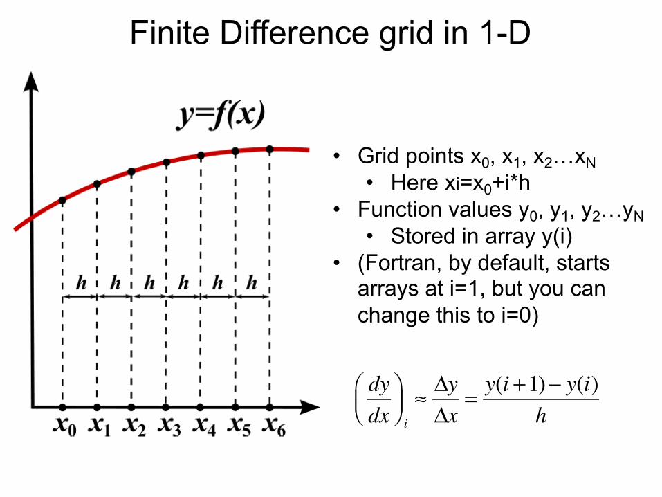
• Grid points x0, x1, x2…xN• Here xi=x0+i*h

• Function values y0, y1, y2…yN• Stored in array y(i)

• (Fortran, by default, starts arrays at i=1, but you can change this to i=0)

Finite Difference grid in 1-D

dydx

⎛⎝⎜

⎞⎠⎟ i≈ ΔyΔx

= y(i +1)− y(i)h

Concept of Discretization• True solution to equations is continuous in

space and time• In computer, space and time must be

discretized into distinct units/steps/points• Equations are satisfied for each

unit/step/point but not necessarily inbetween• Numerical solution approaches true solution

as number of grid or time points becomes larger

Analysis• Subroutine arguments can have

different names from those in calling routine: what matters is order

• FD approximation becomes more accurate as grid spacing dx decreases

• Allocate argument arrays in the calling routine, not in the subroutine/function

Summary: first derivative

• Second derivative

�

dydx

≈ ΔyΔx

= yi − yi−1xi − xi−1

= yi − yi−1h

∂ 2y∂x2

⎛⎝⎜

⎞⎠⎟ i

=yi+1 − 2yi + yi−1

h2

Exercise 3: Second derivative

• Write a subroutine that calculates the second

derivative of an input 1D array, using the finite

difference approximation

• The inputs will be the array, number of points and grid

spacing.

• The resulting 1-D array can be an intent(out) argument.

• The 2nd derivative will be calculated at i=2…n-1

• Assume the derivative at the end points (i=1 and n) is 0.

• Test this routine by writing a main program that

calls the subroutine with two idealized functions for

which you know the correct answer, e.g., sin(x),

x**2. Write out the your code’s result, the correct

result, and the error

• Hand in (to ETHFortran@gmail.com) your .f90

code and the results of your two tests